1

Water vapor measurements by Howard University Raman Lidar during the WAVES 2006 campaign

M. AdamHoward University, Washington, DC, USA

B. B. DemozHoward University, Washington, DC, USA

D. N. WhitemanNASA Goddard Space Flight Center, Greenbelt, Maryland, USA

D. D. VenableHoward University, Washington, DC, USA

E. JosephHoward University, Washington, DC, USA

A. GambacortaPerot System Government Services/NOAA NESDIS, Camp Springs, Maryland,

USA

J. WeiPerot System Government Services/NOAA NESDIS, Camp Springs, Maryland,

USA

M. W. ShephardAtmospheric and Environmental Research, Inc., Lexington, Massachusetts,

USA

https://ntrs.nasa.gov/search.jsp?R=20090019713 2018-05-26T10:09:09+00:00Z

2

L. M. MiloshevichNational Center for Atmospheric Research, Boulder, Colorado, USA

C. D. BarnetNOAA NESDIS, Camp Springs, Maryland, USA

R. L. HermanJet Propulsion Laboratory, California Institute of Technology, Pasadena,

California, USA

J. FitzgibbonNational Weather Service, Sterling, Virginia, USA

R. ConnellHoward University, Washington, DC

__________________

Corresponding author address: Mariana Adam, Howard University, 2355 6th St NW, Washington, DC 20059.E-mail: madam@howard.edu

3

ABSTRACT

Retrieval of water vapor mixing ratio using the Howard University Raman Lidar is

presented with emphasis on three aspects: i) performance of the lidar against collocated

radiosondes and Raman lidar, ii) investigation of the atmospheric state variables when poor

agreement between lidar and radiosondes values occurred and iii) a comparison with satellite-

based measurements. The measurements were acquired during the Water Vapor Validation

Experiment Sondes/Satellites 2006 field campaign. Ensemble averaging of water vapor mixing

ratio data from ten night-time comparisons with Vaisala RS92 radiosondes shows on average an

agreement within 10 % up to ~ 8 km. A similar analysis of lidar-to-lidar data of over 700 profiles

revealed an agreement to within 20 % over the first 7 km (10 % below 4 km). A grid analysis,

defined in the temperature – relative humidity space, was developed to characterize the lidar -

radiosonde agreement and quantitatively localizes regions of strong and weak correlations as a

function of altitude, temperature or relative humidity. Three main regions of weak correlation

emerge: i) regions of low relative humidity and low temperature, ii) moderate relative humidity

at low temperatures and iii) low relative humidity at moderate temperatures. Comparison of

Atmospheric InfraRed Sounder and Tropospheric Emission Sounder satellites retrievals of

moisture with that of Howard University Raman Lidar showed a general agreement in the trend

but the formers miss a lot of the details in atmospheric structure due to their low resolution. A

relative difference of about 20 % is usually found between lidar and satellites measurements.

4

1. Introduction

Water vapor is an important constituent of the atmosphere. The vertical distribution of

moisture is important in determining atmospheric stability. Water vapor is also the most

radiatively active atmospheric trace gas in the infrared (Ramanathan 1988) and thus could

produce strong forcing from feedback associated with anthropogenically driven climate change

(Cess 1990). In addition, there is significant variability in the distribution of water vapor on

temporal and spatial scales smaller than is currently being measured by the standard techniques

(radiosondes, satellites). A better understanding of both the global climatology and the small-

scale variability of water vapor is required to improve simulation of current and future climates

by Global Circulation Models (Moncrieff 1997; Ingram 2002). Without significantly improved

water vapor data, we will continue to be limited in our understanding of important moist

processes within the atmosphere (e.g., Korolev and Mazin 2003; Peter et al. 2006; Demoz et al.

2006).

Routine measurements of atmospheric water vapor have serious limitations. Upper-air

radiosondes are generally launched only twice daily. The quality of the routine global upper air

radiosonde measurement of water vapor is inadequate for many purposes such as radiation

modeling and climate studies (GCOS-121). In the U.S., the data provided by the standard

National Weather Service (NWS) radiosonde sensors can perform poorly in cold dry regions or

when the package becomes wet either in clouds or during precipitation (Wade 1994; Blackwell

1996; Miloshevich et al. 2006). While current satellite remote sensing holds promise for

providing high quality global water vapor observations, it is limited by its vertical and spatial

resolution. Even high quality data from recent satellites (e.g., Aqua and Aura; see http://www-

calipso.larc.nasa.gov/about/atrain.php), do not observe the fine vertical structure of the water

5

vapor. Raman lidars, although generally limited to a single location, provide a high temporal and

spatially resolved water vapor mixing ratio profiles and are capable of continuous measurements

over hours or days (Turner and Goldsmith 1999). This paper discusses the temporal and spatial

retrievals of the water vapor mixing ratio (WVMR) from the Howard University Raman Lidar

(HURL) and its comparisons with satellite, radiosonde, and a Raman lidar. It focuses on three

main aspects: i) the performance of the relatively new HURL system done through comparisons

with collocated Vaisalla RS92 radiosondes and a National Aeronautics and Space

Administration, Goddard Space Flight Center (NASA/GSFC) Raman lidar, ii) a detailed analysis

of the WVMR as measured by lidar and the standard NWS upper air sounding package, the

Sippican Mark IIA radiosonde and iii) a comparisons between HURL and satellites (Aura and

Aqua) retrievals of WVMR. The data used in this paper were collected during the Water Vapor

Validation Experiment Sondes/Satellites (WAVES) experiment that was held at the Howard

University Beltsville Research Campus between 7 July and 12 August 2006. The Howard

University Research Campus is located in Beltsville, Maryland, USA (39N and 76.9W, around

18 km NE of Washington, DC). The objective of WAVES 2006 was to provide i) high quality

measurements of water vapor and ozone profiles for comparison with Aura satellite retrievals, ii)

to assess radiosondes performance and iii) to study upper troposphere water vapor measurements

by Raman lidar systems. The paper is structured as follows. In Section 2, a short description of

the HURL system is provided. Section 3 describes the lidar WVMR calculations. Section 4

presents the data comparison results and discussions. Concluding remarks are presented in

Section 5.

2. Howard University Raman Lidar

6

The Howard University Raman Lidar system was developed to provide both daytime and

nighttime measurements of lower and middle tropospheric water vapor mixing ratios and

aerosol scattering profiling with high temporal and spatial resolution. HURL utilizes a Nd:YAG

laser that operates at the third harmonic wavelength (354.7 nm). HURL is a narrow field-of-

view, coaxial, three-channel, fiber optic-coupled system that uses narrow bandpass (0.25 nm)

filters to measure backscattered radiation at 354.7 nm and Raman scattered radiation from N2

molecules at 386.7 nm and from water vapor molecules at 407.5 nm. HURL utilizes Licel

Transient Recorders (http://www.licel.com/index.html ) for data acquisition that simultaneously

obtain both analog and photon counting signals thereby expanding the dynamic range of the

detection system. The system includes an exit/receiving window that allows operations in

inclement weather. A detailed description of the system is given elsewhere (Venable et al. 2005).

HURL was designed jointly by Howard University and NASA/GSFC and therefore shares some

technologies with that of NASA/GSFC Scanning Raman Lidar (SRL) (Whiteman et a1. 2006a).

The main products of HURL are profiles of WVMR and aerosol backscatter coefficient at high

temporal and spatial resolution (typically, 1 min and 7.5 m). While HURL is not designed to

operate continuously it is capable of operating for extended periods of time, if needed. As

mentioned above, the high temporal and spatial resolution is necessary in the study of the

atmospheric dynamics, especially in the planetary boundary layer (PBL) where the dynamics is

more intense. The Raman lidar products also constitute a source of validation for the satellite

water vapor mixing ratio retrieval. Here, we provide initial comparison examples with retrievals

provided by Atmospheric InfraRed Sounder (AIRS) on Aqua satellite and Tropospheric

Emission Sounder (TES) on Aura satellite.

7

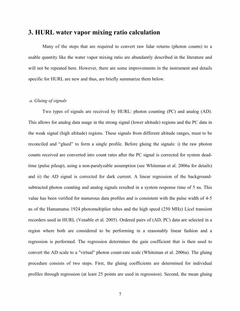
3. HURL water vapor mixing ratio calculation

Many of the steps that are required to convert raw lidar returns (photon counts) to a

usable quantity like the water vapor mixing ratio are abundantly described in the literature and

will not be repeated here. However, there are some improvements in the instrument and details

specific for HURL are new and thus, are briefly summarize them below.

a. Gluing of signals

Two types of signals are received by HURL: photon counting (PC) and analog (AD).

This allows for analog data usage in the strong signal (lower altitude) regions and the PC data in

the weak signal (high altitude) regions. These signals from different altitude ranges, must to be

reconciled and “glued” to form a single profile. Before gluing the signals: i) the raw photon

counts received are converted into count rates after the PC signal is corrected for system dead-

time (pulse pileup), using a non-paralyzable assumption (see Whiteman et al. 2006a for details)

and ii) the AD signal is corrected for dark current. A linear regression of the background-

subtracted photon counting and analog signals resulted in a system response time of 5 ns. This

value has been verified for numerous data profiles and is consistent with the pulse width of 4-5

ns of the Hamamatsu 1924 photomultiplier tubes and the high speed (250 MHz) Licel transient

recorders used in HURL (Venable et al. 2005). Ordered pairs of (AD, PC) data are selected in a

region where both are considered to be performing in a reasonably linear fashion and a

regression is performed. The regression determines the gain coefficient that is then used to

convert the AD scale to a "virtual" photon count-rate scale (Whiteman et al. 2006a). The gluing

procedure consists of two steps. First, the gluing coefficients are determined for individual

profiles through regression (at least 25 points are used in regression). Second, the mean gluing

8

coefficients are determined for each of the aerosol, nitrogen and water vapor profiles and used

for final gluing (see Adam et al. 2007, for further details). The use of the mean gluing

coefficients is beneficial in regions where individual profiles could not be reliably determined

(e.g., in regions where the profiles are affected by clouds).

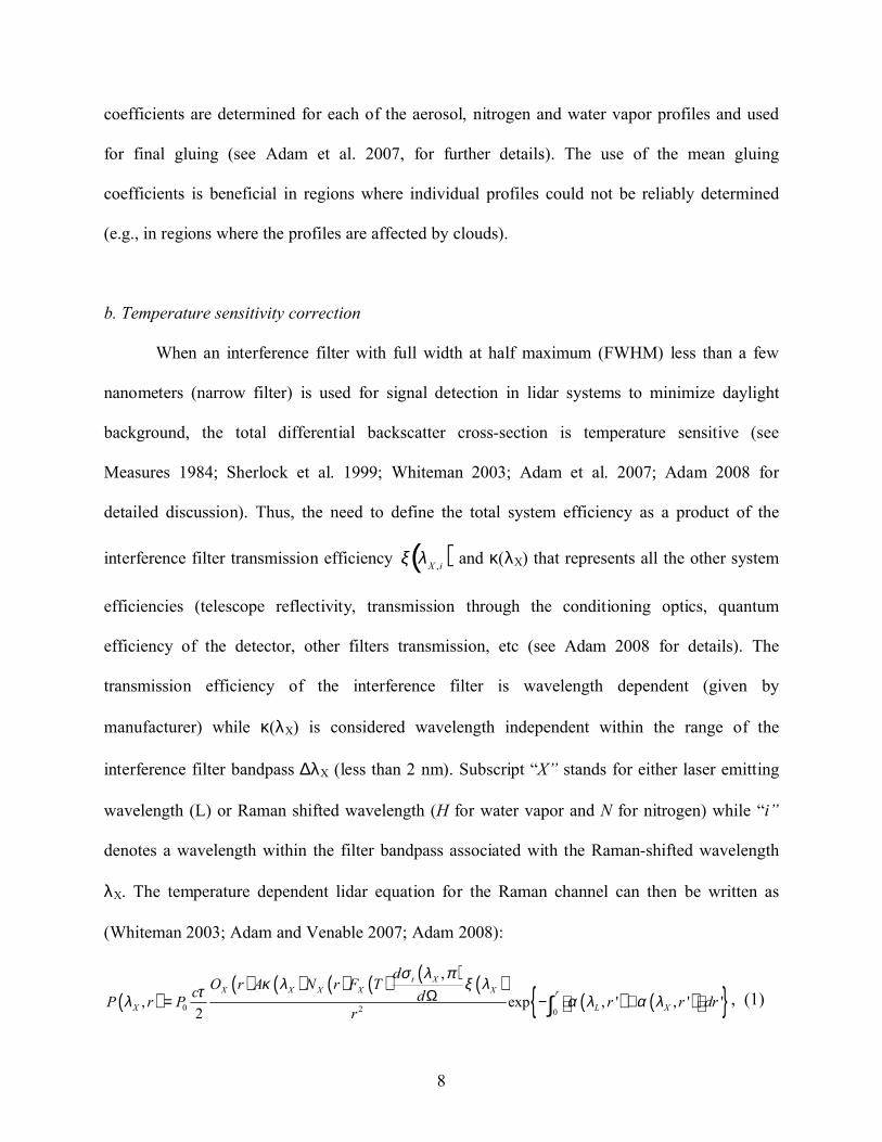
b. Temperature sensitivity correction

When an interference filter with full width at half maximum (FWHM) less than a few

nanometers (narrow filter) is used for signal detection in lidar systems to minimize daylight

background, the total differential backscatter cross-section is temperature sensitive (see

Measures 1984; Sherlock et al. 1999; Whiteman 2003; Adam et al. 2007; Adam 2008 for

detailed discussion). Thus, the need to define the total system efficiency as a product of the

interference filter transmission efficiency ξ λX ,i( ) and κ(λX) that represents all the other system

efficiencies (telescope reflectivity, transmission through the conditioning optics, quantum

efficiency of the detector, other filters transmission, etc (see Adam 2008 for details). The

transmission efficiency of the interference filter is wavelength dependent (given by

manufacturer) while κ(λX) is considered wavelength independent within the range of the

interference filter bandpass ∆λX (less than 2 nm). Subscript “X” stands for either laser emitting

wavelength (L) or Raman shifted wavelength (H for water vapor and N for nitrogen) while “i”

denotes a wavelength within the filter bandpass associated with the Raman-shifted wavelength

λX. The temperature dependent lidar equation for the Raman channel can then be written as

(Whiteman 2003; Adam and Venable 2007; Adam 2008):

( )( ) ( ) ( ) ( ) ( ) ( )

( ) ( ) 0 2 0

,

, exp , ' , ' '2

t XX X X X X r

X L X

dO r A N r F Tc dP r P r r dr

r

σ λ πκ λ ξ λτ

λ α λ α λΩ= − + ∫ , (1)

9

P(λX) is the backscatter power [W], P0 is the outgoing laser power [W], c is the speed of light [m

s-1], τ is the pulse duration [s], OX(r) is the overlap function [dimensionless], A/r2 is the solid

angle [sr] defined by the telescope area A [m2] and the distance r [m] from the lidar to

backscatterer. NX is the number of molecules of the X species, α is the extinction coefficient at

laser wavelength λL and Raman shift wavelength λX and OX is the overlap function at

wavelength λX. The exponential term represents the round trip transmission from the lidar to the

backscatter (molecule or particle). The total extinction coefficient α is the sum of molecular and

aerosol components [m-1]. The molecular backscatter coefficient is the product of the total

number of molecules NX (calculated from radiosondes pressure and temperature measurements)

and the total molecular differential backscatter cross-section dσt(λL,π)/dΩ [m2 sr-1]. The later is

the sum of all individual cross-sections over Q, S and O branches (Raman vibrational-rotational

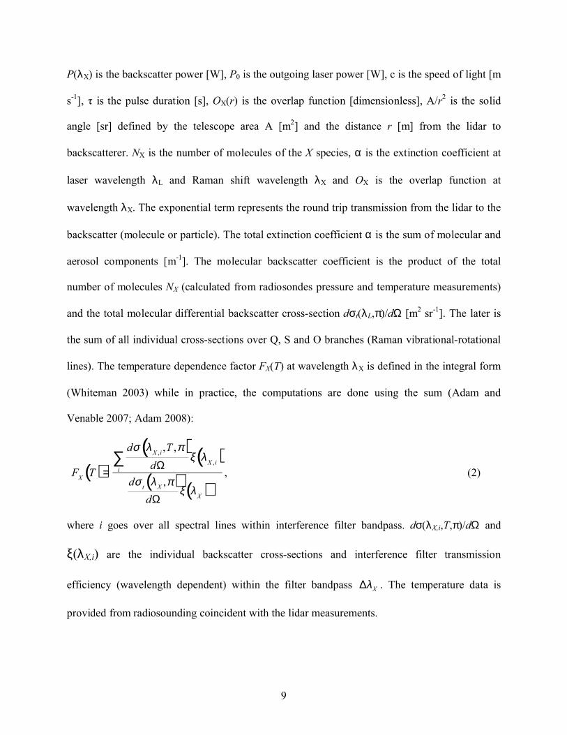
lines). The temperature dependence factor FX(T) at wavelength λX is defined in the integral form

(Whiteman 2003) while in practice, the computations are done using the sum (Adam and

Venable 2007; Adam 2008):

FX T( )=

dσ λX ,i ,T ,π( )dΩ

ξ λX ,i( )i

∑dσ t λX ,π( )

dΩξ λX( )

, (2)

where i goes over all spectral lines within interference filter bandpass. dσ(λX,i,T,π)/dΩ and

ξ(λX,i) are the individual backscatter cross-sections and interference filter transmission

efficiency (wavelength dependent) within the filter bandpass Xλ∆ . The temperature data is

provided from radiosounding coincident with the lidar measurements.

10

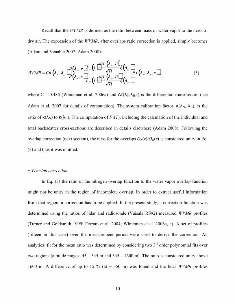
Recall that the WVMR is defined as the ratio between mass of water vapor to the mass of

dry air. The expression of the WVMR, after overlaps ratio correction is applied, simply becomes

(Adam and Venable 2007; Adam 2008):

WVMR = Cκ λN ,λH( )P λH ,r( )P λN ,r( )

FN T( )dσ t λN ,π( )dΩ

ξ λN( )

FH T( )dσ t λH ,π( )dΩ

ξ λH( )∆τ λN ,λN ,r( )., (3)

where C ≅ 0.485 (Whiteman et al. 2006a) and ∆τ(λN,λH,r) is the differential transmission (see

Adam et al. 2007 for details of computation). The system calibration factor, κ(λN, λH), is the

ratio of κ(λN) to κ(λH). The computation of FX(T), including the calculation of the individual and

total backscatter cross-sections are described in details elsewhere (Adam 2008). Following the

overlap correction (next section), the ratio for the overlaps ON(r)/OH(r) is considered unity in Eq.

(3) and thus it was omitted.

c. Overlap correction

In Eq. (3) the ratio of the nitrogen overlap function to the water vapor overlap function

might not be unity in the region of incomplete overlap. In order to extract useful information

from that region, a correction has to be applied. In the present study, a correction function was

determined using the ratios of lidar and radiosonde (Vaisala RS92) measured WVMR profiles

(Turner and Goldsmith 1999; Ferrare et al. 2004; Whiteman et al. 2006a, c). A set of profiles

(fifteen in this case) over the measurement period were used to derive the correction. An

analytical fit for the mean ratio was determined by considering two 3rd order polynomial fits over

two regions (altitude ranges: 45 – 345 m and 345 – 1600 m). The ratio is considered unity above

1600 m. A difference of up to 15 % (at ~ 350 m) was found and the lidar WVMR profiles

11

corrected accordingly. An additional improvement in the overlap correction and water vapor

mixing ratio data quality was achieved, by minimizing reflections in the laboratory of the elastic

signal, which we speculate contaminated the nitrogen and water vapor channels also. This new

configuration of the system, which includes a baffle which shielded the transmitted laser beam

from the telescope to the exit/receiving window, eliminated the observed strong increase in the

elastic channel backscatter signal and the deviation from unity of the lidar-sonde WVMR ratio

above 400 m.

d. Raman lidar calibration factor

Further, routine calibration of lidar measured water vapor mixing ratio data by tracking

the calibration factor, κ(λN,λH) in Eq. 3, is performed by comparison of the night time lidar

integrated precipitable water (IPW) measurements with IPW measured using a microwave

radiometer (MWR) as is routinely done in Raman lidar calibration (see for example; Turner and

Goldsmith 1999; Turner et al. 2002; Ferrare et al. 2004; Whiteman et al. 2006a; Adam and

Venable 2007). The MWR IPW is assumed to be reliable, with its uncertainty in the range

0.2mm – 0.4mm, depending on absolute value of IPW (Cimini 2003). The absolute IPW

measurements observed during WAVES 2006 campaign varied between 10 mm and 60 mm,

with most of the values being above 20 mm. Consequently, expected errors for the MWR IPW

are less than 2 %. The MWR to lidar IPW ratio is required for the lidar calibration factor for

water vapor mixing ratio. For each period analyzed, as a first step, the mean and the standard

deviation (STD) of the lidar calibration factor are computed and the outliers (larger than

STD/mean = 0.01) excluded. With the remaining set of calibration factors, a new mean and STD

are computed. The mean calibration factor is then used for the calibration of all the profiles

12

during that period. As in the case of gluing coefficients, this assures that a calibration factor is

obtained even in regions where it cannot be reliably calculated due to cloud or other reasons. For

the entire WAVES 2006 campaign, the mean calibration factor is ~ 501.97 g/g while the STD is

~ 15.68 g/g. The corresponding relative error (100 STD/mean) is found to be 3.12 %. Variation

of the calibration factor has been reported for a number of Raman lidar systems; for example, in

the case of absolute Raman calibration, Sherlock et al. (1999) reported a 10 - 12 % uncertainty.

For radio sounding based calibration (using RS80 type sondes), Ferrare et al. (1995) reported a 1

% change but when an Atmospheric Instrumentation Research (AIR) radiosonde was used the

calibration changed by 5% over two years. Using a Meisei RS2-91 type of radiosonde, Sakai et

al. (2007) reported an 11 % change over 18 months. Whiteman et al. (2006a) report a 6 %

change when calibration was performed with GPS IPW. Variation of the calibration factor (3 %),

when performed with respect to a MWR IPW is reported by Turner and Goldsmith (1999) who

combine two intensive campaigns over 1996 and 1997. The comparisons were made over ten

minute averages and finally collected into 30 min bins. Ferrare et al. (2004) compared seven

airborne based lidar IPW with ground based MWR and found a 3 % change (a variable

smoothing was applied to lidar data to constrain the random error within 2 – 5 %). The HURL

calibration constant variations reported here fall in the low range of variation in the calibration

constants reported, an indication of the stability of the system over time. Because system

performances are expected to change over time (degradation of components, laser power, etc),

the variation will be tracked over the HURL lifetime.

4. Data, results and discussions

13

The WAVES 2006 field campaign took place at the Howard University Research

Campus in Beltsville, MD, USA from July 7 to August 10. Groups from thirteen academic and

government institutions participated. The key government collaborators included groups from

National Ocean and Atmospheric Administration (NOAA) / NWS and NASA/GSFC. The field

campaign was intended to provide high quality measurements of water vapor and ozone for

validation of Aura satellite retrievals, to assess the accuracy of upper tropospheric water vapor

measurements using radiosounding and to observe mesoscale processes that influence local air

quality and regional water vapor variability. The operations include intensive observations by

multiple radiosonde/ozonesonde sensors and several lidar systems during overpasses of Aura and

other A-Train satellites. In addition to the lidar/radiosondes operations, continuous

meteorological measurements were recorded using a suite of sensors: a 31 m instrumented tower

(for temperature, pressure, relative humidity, flux and wind); various broad-band and spectral

radiometers; a 2-channel microwave radiometer; a Doppler C-band radar; various aerosol

chemical parameters; a 915 MHz wind profiler operated by the Maryland Department of

Environment (MDE), a sun photometer (operated by the US Agricultural Services and a part of

AERONET network), and a Suominet GPS system. More information can be found on the

WAVES webpage http://www.ecotronics.com/lidar-misc/waves_06/waves06.htm.

Satellite validation is often preferred in homogeneous locations: over water or at

locations where pollution is low and surface albedo has been well characterized (e.g. Tobin et al.

2006). The Beltsville facility is located in a high population area and major pollution corridor in

the Eastern US. It belongs to a semi-urban region where a wide range of meteorological

conditions occurs though out the year. It provides an environment very different than ARM sites.

Also, great opportunities for inter-agency and university collaboration exists (e.g. HU - MDE –

14

NOAA – NASA). The atmospheric measurement program at Beltsville has developed expertise

in upper air ozone sounding over the past several years through participation in the INTEX

Ozonesonde Network Study (IONS) (Thompson et al. 2007) and the State of Maryland

Department of the Environment summer air quality monitoring campaigns.

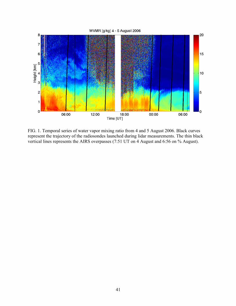
The HURL system operated over a 14 day period between July 7 and August 12 of 2006

as part of WAVES 2006. Figure 1 shows an example of a time-series of WVMR (g kg-1) profile

data covering around 30.5 hours: starting at 00:50 UT on 4 August 2006 and ending at 07:21 UT

on 5 August 2006. Temporally, convective clouds were present at the top of the PBL (better seen

in aerosol backscatter ratio; see http://meiyu.atmphys.howard.edu/~adam/HRL_WAVES.html),

specifically over the first 3 hours and during daytime operation, ~ 12:00 and 19:30 UT on 4

August. The data gap at 16:00 UT on 4 August is due to HURL interruption due to heavy

rainfall. The temporal resolution of the data is 1 min while the vertical resolution is 30 m. No

smoothing was applied to the data. The data represent the passage of a cold front over the site,

which cleared the PBL moisture after about 00:00 UT on 5 August 2006. Note also the highly

variable WVMR structure in the boundary layer revealed by the Raman lidar data. A rigorous

study of this case supported with modeling is in progress and will be reported elsewhere. It is

shown here i) as an illustration of the HURL capability and ii) to add temporal context to

comparisons of HURL and radiosonde water vapor mixing ratio profile comparison from this

case discussed below. In summary, a total of 133 HURL operational hours of data were

collected, of which 84 hours were during night-time and 49 hours were during day-time. Several

types of radiosonde packages, collocated Raman lidars and satellite data sets were also operated.

A comparison of the HURL data with these data sets is discussed in the following section.

15

a) System performance. HURL – Vaisala radiosonde (RS92) comparisons

Ten comparisons with Vaisala RS92 radiosondes were available for night-time

operations. However, prior to comparing lidar – sonde data values, the RS92 relative humidity

(RH) measurements were corrected for known measurement errors using an algorithm similar to

the time-lag and empirical bias correction described by Miloshevich et al. (2006). The RS92 data

were first corrected for time-lag error (slow response of the RH sensor at low temperatures)

based on laboratory measurements of the sensor time-constant as a function of temperature

(Miloshevich et al. 2009). Then an empirical correction for mean calibration bias was applied,

which was derived as a function of RH and altitude from dual RS92/CFH (Cryogenic Frost point

Hygrometer) soundings conducted during several experiments (including WAVES). These

corrections resulted in a mean accuracy of about ±(4% + 0.5%/RH) for all RH conditions

throughout the troposphere and a standard deviation of RS92-CFH differences of about 5%

(Miloshevich et al. 2009). The RS92 calibration bias below the 700 mb level was derived in part

from comparisons of RS92 to collocated MWR retrievals of IPW using the latest MWR physical

retrieval algorithm (Turner et al. 2007). Daytime RS92 measurements are also affected by a solar

radiation error, which is often a dry bias caused by solar heating of the RH sensor (Vömel et al.

2007). A daytime RS92 correction for RH and height dependence of solar radiation error is

derived from dual RS92-CFH dual soundings and dependencies of the error on the solar altitude

angle is derived from the day-night difference between the RS92 and MWR measurements, with

results similar to those of Cady-Pereira et al. (2008).

In forming the HURL-RS data pairs for comparison, the lidar profiles are selected

according to the radio sonde trajectory (a process referred to as RS tracking) and are shown by

black lines on Fig. 1 (note: dashed line indicate time of Aqua satellite overpass). The assumption

16

in forming the RS tracking is that at each moment (time stamp) the atmosphere is horizontally

homogeneous to account for possible horizontal shifts in the RS trajectory. A version of this

technique was described by Whiteman et al. (2006c) and used during the AIRS Water Vapor

Experiment (AWEX) campaign, where the authors applied a variable smoothing to the lidar data.

In this case, a moving average was performed over 5 temporal profiles. An additional moving

average over 31 minutes was applied for altitudes higher than 5 km. A variable vertical

smoothing was performed as follows: for altitude ranges of 1-2 km, 2-4 km, 4-6 km, 6-8 km, 8

km-up a moving average over 3, 5, 7, 9 and 11 bins, respectively, was performed (each bin

represents 30 m). In cases of temporally homogenous data sets, the RS tracking method gives

similar results to the non-tracking averages (averaging time starts at RS launch time). In cases

where there is significant atmospheric temporal variability over the course of the RS flight, large

difference is found between the two methods. Consequently, the RS tracking method is used for

the lidar comparison with RS. Our current methodology to track RS is based on two steps. First,

mean values of the RS data are calculated for each layer corresponding to a lidar altitude bin (30

m). Next, the lidar data are linearly interpolated to match the RS time stamps corresponding to

the RS means calculated in the first step. Two profile comparisons using data from Fig. 1 (the

fourth and the last RS trajectories with launch times at 23:13 UT on 4 August and 06:01 UT on 5

August), are discussed to demonstrate HURL-RS92 comparisons (Figs. 2-3). The water vapor

mixing ratio from two sensors on the meteorological tower (MT), at 1.5 and 31.8 m, are also

shown as asterisks in the figures.

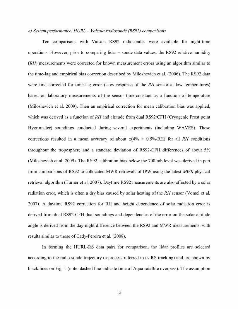
In the first example, the lidar retrieval in Fig. 2 is limited to about 3 km because of low

signal to noise ratio (SNR) above this altitude due to daytime solar noise. In the first 2 km, an

agreement within 5 % is found degrading at higher altitudes mainly due to low lidar SNR (see

17

also larger error bars in this region). The solid black curve and the error bars represent the mean

relative difference and STD over 500 m blocks while the dotted curve represents the mean

relative difference at 30 m resolution [Fig. 2(b)]. The maximum drift reached by the radiosonde

(4.8 km) occurred at an altitude of 3.25 km, the highest altitude considered for comparison in

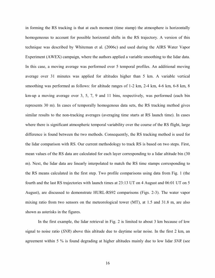
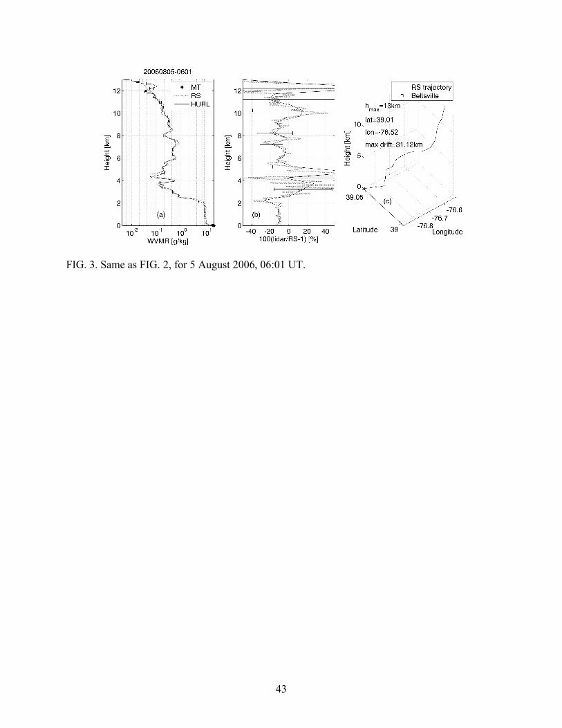
Fig. 2 (c). In the second example (Fig. 3), on average, the sonde profile is 10 % moister than the

lidar profile. Larger differences are found in the region between 2 and 5 km as well as above 10

km, when the sonde drifted farther away (~ 13 km). Note that between 2 and 5 km, RH is ≤ 3 %

which translates into a RS uncertainty of 21 %.

The profile comparisons shown above demonstrate the range of variability that can occur

when comparing lidar-sonde profiles, even within this relatively short time difference. This

variability in lidar-sonde differences can be due to a combination of factors: sensor performance

and/or atmospheric variability. One way of minimizing these effects of variability is to perform

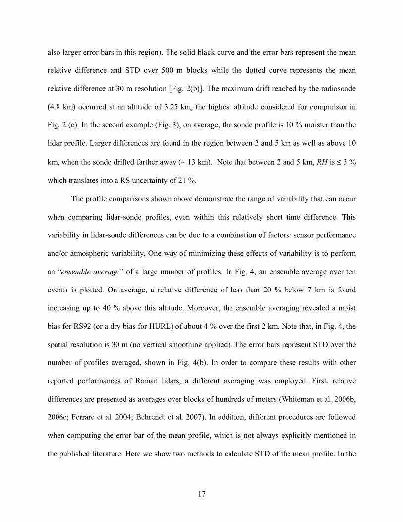
an “ensemble average” of a large number of profiles. In Fig. 4, an ensemble average over ten

events is plotted. On average, a relative difference of less than 20 % below 7 km is found

increasing up to 40 % above this altitude. Moreover, the ensemble averaging revealed a moist

bias for RS92 (or a dry bias for HURL) of about 4 % over the first 2 km. Note that, in Fig. 4, the

spatial resolution is 30 m (no vertical smoothing applied). The error bars represent STD over the

number of profiles averaged, shown in Fig. 4(b). In order to compare these results with other

reported performances of Raman lidars, a different averaging was employed. First, relative

differences are presented as averages over blocks of hundreds of meters (Whiteman et al. 2006b,

2006c; Ferrare et al. 2004; Behrendt et al. 2007). In addition, different procedures are followed

when computing the error bar of the mean profile, which is not always explicitly mentioned in

the published literature. Here we show two methods to calculate STD of the mean profile. In the

18

first method, the mean of the relative difference is computed for each profile and for each block

and then the mean relative differences computed (similar to Whiteman et al. 2006b). In the

second method, for each block, STD is computed taking into consideration all the measurement

points available (the population) from all available profiles (similar to Ferrare et al. 2004). Figure

4(c) shows the relative difference and the STD determined by the two methods using 500 m

blocks in altitude. We can infer that the thick error bars (method I), can be associated with the

atmospheric vertical variation while the thin error bars (method II) can be associated with both

vertical and temporal atmospheric heterogeneity. The mean HURL-RS92 water vapor mixing

ratio relative difference is less than 10 % over the entire region, except the uppermost block. This

represents a very good result as compared with similar comparisons reported.

b) System performance: HURL –SRL intercomparisons

HURL and the NASA/GSFC SRL (Whiteman et al. 2006a) were operated side by side. This

setup provided an opportune time for HURL-SRL comparison because of the proximity of the

lidars and because of the similar technical characteristics of the lidars. The SRL operates using

the third harmonic Nd:YAG laser, and acquires data at 354.7 nm, 386.7 nm and 407.5 nm. It has

a frequency of 30 Hz and uses PC and AD acquisition. In addition to the water vapor mixing

ratio and aerosol backscatter, it also measures depolarization and liquid water content using two

telescopes: a 25 cm (high channel) and 76 cm (low channel). The SRL is a well-established

instrument with a long history of making successful measurements of tropospheric water vapor

(see Whiteman et al. 2006a-c and references within). The SRL water vapor mixing ratio for the

high channel was calibrated using the same MWR used for HURL. For the period analyzed (3

August 2006), there are almost 13 hours (766 profiles) of coincidental measurements. Figure

19

5(a)-(b) shows an example of individual profile comparison. A temporal and vertical smoothing

was applied for both lidar data as follows. First, a temporal moving average over 11 min is

applied at all altitudes. Next, an additional temporal moving average over 11 profiles is applied

for altitudes above 5 km. Finally, the same vertical smoothing as in the case of HURL-RS92 case

is applied. The thick curve and error bars [Fig. 5(b)] represent the mean and STD over 500 m

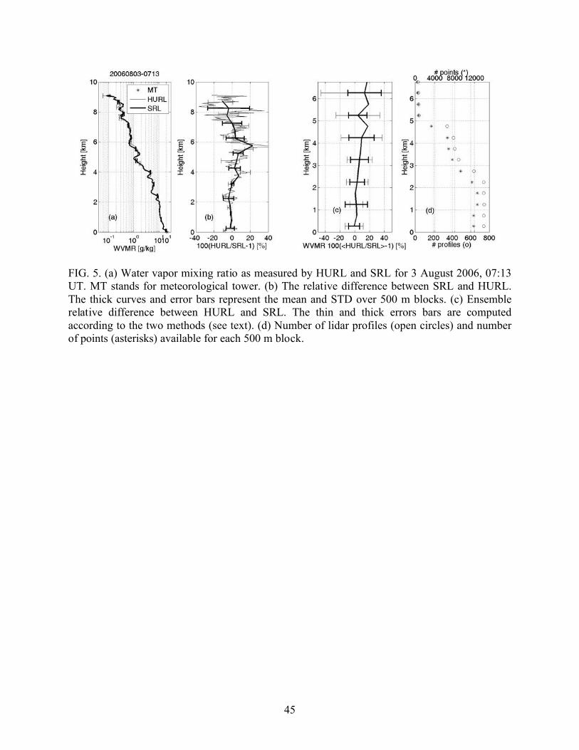
blocks. On average, a 10 % agreement was found between the lidars, except in the altitude range

between 5.5 and 6 km. Note that the SRL has a better SNR at high altitudes because it operates

using a more powerful laser. Ensemble average is also performed over a maximum of 766

profiles (in the lower troposphere) with no vertical smoothing applied [Fig. 5(c)]. The error bars

corresponding to the relative differences are computed using the two methods described above.

Several additional criteria were followed in computing the mean profiles and their relative

difference. First, the lidar profiles are restricted to a region where the noise did not overwhelm

the signal, choosing only the region where the WVMR is always positive. Second, only points

with relative error (100 STD/mean) smaller than 30 % are taken into consideration.

Consequently, out of the maximum available number of profiles in the lower troposphere (766),

only 30 profiles survived this restricted conditions at high altitudes [circles in Fig. 5(d)]. A

similar decrease occurs for the number of points when the data are averaged over 500 m blocks

[asterisks in Fig. 5(d)]. A mean relative difference of less than 10 % below 4.5 km increasing to

less than 20 % over all altitude ranges is found. In addition, HURL WVMR profiles were moister

(biased) above 2 km which at present is not explained. Further investigation is required to

understand this behavior.

c) Grid method

20

Numerous comparisons of lidars and radiosondes derived water vapor mixing ratio are

reported in the literature. Most of these comparison studies are presented either as profile by

profile, ensemble averages or as IPW correlations. The effects of temperature and relative

humidity on instrument performance are often studied separately. To visualize the instrument

error characteristics in a unified form, a grid method is developed. This method is used to

investigate the meteorological conditions (in terms of temperature and relative humidity) under

which poor agreement occurs between the lidar and radiosonde profiles. In the present paper, the

method is applied to HURL and NWS Mark IIA sondes. This study is part of a NOAA Center for

Atmospheric Sciences (NCAS) and NWS long-term collaboration as part of the NWS’

radiosonde testing and replacement program. The goal is to validate the new sensors using

HURL and other supporting observations that are performed at Beltsville. Two examples, typical

of the data during this campaign, are used (Figs. 6-7) to demonstrate the method. The temporal

smoothing applied to HURL data is the same as done above in the case of HURL-RS92

comparisons. However, no vertical smoothing is applied, keeping a 30 m spatial resolution over

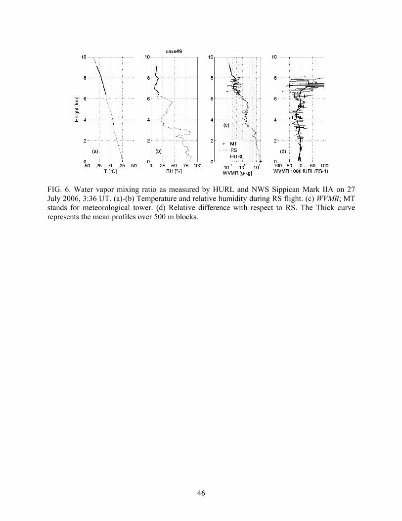
the entire altitude range of the analysis. The first example, from 03:36 UT on 27 July 2006, is

representative of the good comparisons with relative differences below 20 % up to 6 km, and

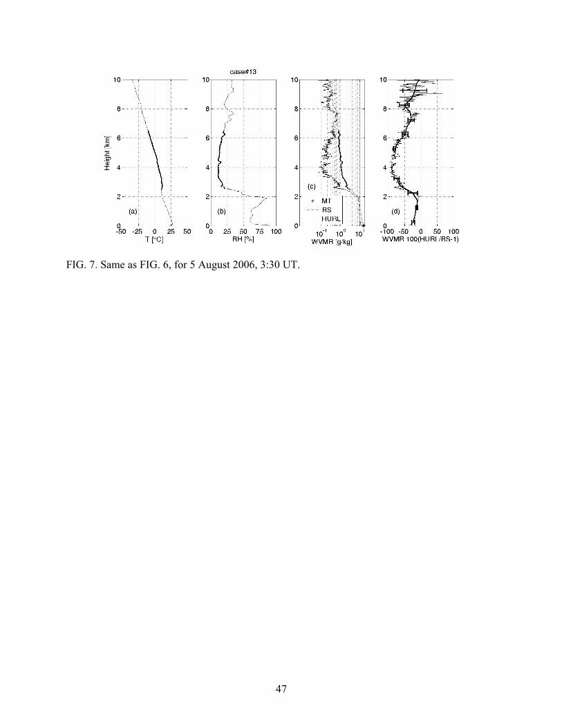
much smaller below 2 km [Fig. 6(a-d)]. The second example, taken from 5 August 2006 at 03:30

UT, is a poor case of comparison where there is relatively large moist bias between HURL and

the Mark IIA sonde data [Fig. 7(a-d)]. The thick curves in Figs. 6(d) and 7(d) plots represent the

mean and STD of the relative difference computed for 500 m blocks.

As is evident from Fig. 1, the lidar revealed a dry region between 2 and 6 km, where the

mixing ratio decreases above the boundary layer. In such dry regions, the accuracy of the Mark

IIA derived relative humidity shows substantial errors and was observed in several profiles. This

21

limitation of the Mark-IIA may be a result of the errors in calibration, sensor hysteresis, and

sensor response time (Blackmore and Taubvurtze 1999). According to Blackmore and

Taubvurtze (1999), at low temperatures, the calibration (lock-in resistance) increases while the

time response slows. Low temperatures and sensor hysteresis cause errors up to 10 % in RH. At

transition from high to low RH, the sensor hysteresis can also induce errors within 10 % in RH

(drier RH). However, the present study reveals a much larger mixing ratio differences at the

transition between high to low RH. These findings are consistent with those reported by Ferrare

et al. (2004) and Sakai et al. (2007). Da Silveira et al. (2001) reported substantial large

disagreements between Mark IIA and other sensors in their study of GPS-sonde intercomparison

while Wang et al. (2003) reported time-lag errors and failure of the sonde to respond to humidity

changes in the upper and middle troposphere. Miloshevich et al. (2006) report slow time

response at low temperatures and a moist bias in middle troposphere of 10 - 30 % as compared

with RS80-H. These authors consider the measurements to be suspect between -20°C and -50°C

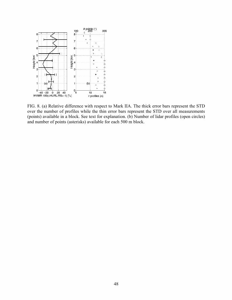
and all temperatures when operated under dry conditions. Ensemble average plots in Fig. 8,

clearly show the above findings; a large moist bias for sonde is revealed between ~ 2.5 and 5.5

km.

Since the atmosphere can have several cold-dry regions as well as fast RH transition

areas that result in large differences, a grid analysis in the dual variables, temperature – relative

humidity (T – RH), space was developed. This allows for quantification and easy visualization of

instruments (dis)agreement, here expressed as the WVMR root mean square error (RMS). Note

that the temperature and relative humidity are provided by the radiosondes and the focus here is

on large discrepancies, (large RMS) between the two instruments. The methodology is as

follows: for each increment of ΔT = 10 °C and ΔRH = 10 % we compute RMS as:

22

21100 1 [%]HURL

n RS

WVMRRMSn WVMR

= −

∑ , (4)

where n represents the number of WVMR data points within each ΔT and ΔRH space. The RMS

is then contoured in T – RH space as shown in Figs. 9 and 10. The first case shows that the

largest RMS occurs for ΔT = [-30, -20] °C and ΔRH = [10, 20] %, i.e. in cold and dry regions.

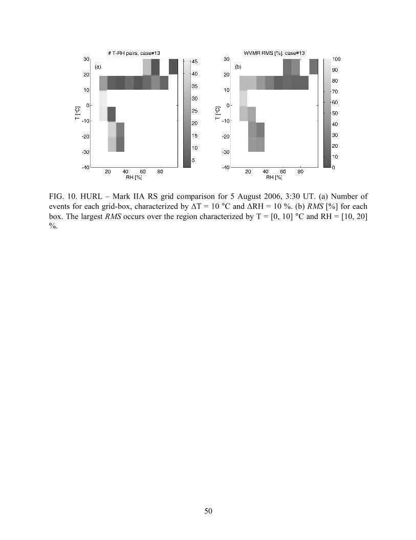
The second case shows the largest RMS in the region characterized by ΔT = [0, 10] °C and ΔRH

= [10, 20] %. Relative large RMS (> 0.5) occur also in boundary layer region (relatively warm

and moist), characterized by ΔT = [10, 20] °C and ΔRH = [10, 30] %. Note again that this

mapping of RMS into the T - RH space can be easily reversed and the T-altitude and RH-altitude

pairs can be extracted. A plot of the data points for which RMSthreshold=0.5 are shown in Figs. 6 –

7 by dots on the curves; shown as heavy lines. Thus, the box with the largest RMS in Fig. 9

corresponds to the thick part of the curve shown in Fig. 6 (~ 6.5-9 km). Similarly, for Fig. 10, the

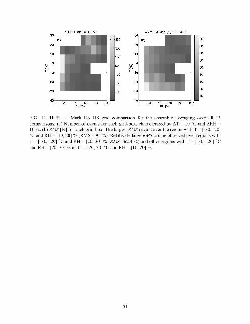
regions with RMS > 0.5 correspond to the thick curves in Fig. 7 (~2.5-6.5 km). In summary, the

ensemble averaging of the RMS (Fig. 11) reveals the largest HURL-Mark IIA discrepancies over

cold and dry regions, characterized by ΔT = [-30, -20] °C and ΔRH = [10, 20] %, where RMS

reaches ~ 93 %. Relatively large values (> 0.5) also occur elsewhere where RH < 60 % while T

varies. Note the box where ΔT = [10, 20] °C which suggest that the region is somewhere within

the boundary layer. Note also that the differences in cold and dry regions should not be attributed

to Mark IIA sonde (inadequate RH sensor response at low T) alone; lidars also are affected by

the low SNR and low quantity of water vapor molecules. In other conditions, the difference is

primarily attributed to the inadequacies in Mark IIA RS sensor response in high gradient

moisture regions (as from high to low RH). More detailed analyses can and should be performed

23

by choosing a higher resolution grid defined by smaller ∆T and ∆RH intervals than used here,

provided that a statistically significant number of data points exist for each grid-box.

c) WVMR HURL-satellites

As mentioned above, one of the main objectives of the WAVES campaign was to provide

ground-based measurements for the validation of the Aura sensors. However, since both Aura

and Aqua overpass occurs only 15 minutes apart, both are studied. The WVMR profiles derived

from lidar are compared with those from TES on Aura and AIRS on Aqua satellites (for details

and publications on AIRS and TES, please visit http://www-airs.jpl.nasa.gov/Documents and

http://tes.jpl.nasa.gov/docsLinks/index.cfm, respectively). In brief, AIRS was launched to

provide temperature and water vapor profiles or spectral radiances for assimilation in numerical

weather prediction and to provide an improved understanding of the atmospheric branch of the

hydrological cycle and climate processes (Auman et al. 2003; Fetzer 2006; and references

therein). An ultimate goal of the AIRS validation effort is to achieve WVMR RMS uncertainties

of 10 % over 2 km layers in troposphere (Fetzer et al. 2003; Tobin et al. 2006). For TES, the

main objective is to measure the global profiles of tropospheric ozone and its precursors, among

which water vapor is particularly important (Shephard et al. 2008 and references therein). The

criteria used for selection of profiles in this study are such that the Aura satellite ground track

lies within 50 km of the Beltsville site. Note also that the day-time comparisons were restricted

to below 5 km altitude, due to low SNR in the lidar signals or due to the presence of convective

clouds in the boundary layer, while at night the altitude range for comparison extended on

average to 10 km.

AIRS Version 5 tropospheric moisture retrieval resolution as determined by the FWHM

of the averaging kernels ranges between 2.7 km near the surface and 4.3 km near the tropopause

24

(Maddy and Barnet 2008), which is similar to TES performance (Shephard et al., 2008). In

addition, AIRS moisture retrieval degrees of freedom for nominal mid-latitude cases is nearly

4.0, which is also very close to the TES moisture retrieval reported in Shephard et al., [2007].

We therefore would expect similar performance in the AIRS and TES water retrievals if we

accounted for the a priori dependence of the AIRS retrievals using averaging kernels (Maddy and

Barnet, 2008). For consistency with previous AIRS water vapor validation efforts (Whiteman et

al. 2006c), we have chosen to compare the AIRS retrievals using traditional simple layer

techniques (i.e., without the use of averaging kernels). In this study, AIRS level2 products are

used where temperature and water vapor profiles are reported on a 100 vertical grid layers. The

calculation of mean mixing ratio within a layer takes into account the conservation of the number

of molecules within each layer (http://www.osdpd.noaa.gov/PSB/SOUNDINGS/ORA/AIRS_

barnet.pdf) and is given by the ratio of the water vapor to dry air column densities.

The TES temperature and water vapor volume mixing ratio are reported on a standard 67-

pressure level grid. The TES footprint, at Nadir, is 8x5km. TES utilizes an optimal estimation

retrieval approach to simultaneously minimize the difference between observed and model

spectral radiances in order to estimate atmospheric profiles (Bowman et al. 2006). Provided with

each TES retrieved profile is the corresponding averaging kernel, which describes the sensitivity

of the retrieval. The FWHM of the rows of the averaging kernels provide the vertical resolution

of the retrieval. To help provide some additional insight, the sum of the rows of the averaging

kernels can be thought of as the fraction of information in the retrieval that comes from the

measurement rather than the a priori. Note that the sensitivity of TES varies profile-to-profile

depending on atmospheric state (concentration of the species of interest, temperature, etc),

clouds, and constraints used in the retrieval. Since the goal of these comparisons is to validate the

25

satellite measurements, the TES averaging kernels and a priori profile were applied to the sondes

and/or lidar profiles in order to account for the a priori bias, sensitivity and vertical resolution of

the TES retrievals (Shephard et al. 2008). The TES standard procedure maps the in situ

measurements (radiosonde or lidar) to the TES reported grid levels, and then applies the TES

averaging kernels Axx and the a priori profile Xa to the mapped in situ profile X insitumapped :

X insituest = Xa + Axx X insitu

mapped − Xa( ), (5)

Using this method we obtain a lidar or radiosonde profile that represents what TES would “see”

for the same atmospheric state (thus yielding a profile that accounts for TES sensitivity and

vertical resolution). The TES vertical resolution, computed at FWHM of the averaging kernels

(Shephard et al. 2008) is ~2 km from the surface up to close to 4 km, ~3 km between 4 km and

close to 8 km, and 3.5 – 4 km between 8 km and 11 km.

During the WAVES 2006 campaign, 13 coincidences were found for AIRS-HURL water

vapor mixing ratio comparison. Two examples of such a comparison for the night-time cases (4

August, overpass time 07:51 UT and 5 August, overpass time 06:56 UT) are shown in Fig. 12.

The averaging was performed over 2 km layers in order to have a direct comparison with

previous studies by AIRS community (e.g. Tobin et al 2006). The average over the 2 km layer

was performed as following. Within each 2 km layer, the mean value was determined as the

integral of all available points in the layer divided by the thickness of the layer (2 km). The

common practice in the AIRS community of weighting the statistics by the water vapor layer

amounts was not applied here, thus the relative differences between the lidar and AIRS are more

comparable to the larger non-weighted results reported by Tobin et al. (2006). The Aura ground

track was 48.5 km away from Beltsville on 4 August and 30.96 km on 5 August. In addition, the

HURL-derived time-height evolution of mixing ratio (Fig. 1) during the overpass time shows a

26

strong temporal and vertical variability over the region, including the presence of dry and moist

layers above (e.g. ~ 3 km, 5 - 6 km). Note that in averaging the HURL data in 2 km layers in

order to compare with the AIRS resolution removes a lot of the atmospheric variability and the

small scale structures in the profile. The HURL/AIRS comparisons show relative differences

below 20 % for the 4 August case. For the August 5 case, large differences occur around 3 km,

most likely associated with the frontal surface variability. As can be seen in the original HURL

profile (and also in Fig. 1), the lidar reveals a quick reduction in the water vapor mixing ratio

results above the elevated moist layer lifted due to the cold frontal surface (above 2km). Thus,

the layer averaged value in the 2-4 km altitude region is much smaller than the retrieved value by

AIRS, which has a much wider footprint as discussed above. On average, AIRS captures the

general shape of the lidar profiles, but fails to catch the finer atmospheric layers due to its

inherent lower spatial resolution. Note also that the small scale structures reported by HURL

during this time are also present in the RS data at 06:00 UT. Moreover, the values recorded at the

meteorological tower (at 1.5 m and 31.8 m) agree with lidar and RS data close to the ground. In

the past, relative difference up to 30 % between AIRS and SRL is reported by Whiteman et al.

(2006c) for ensemble average and over a variable vertical resolution (1 km layers below 4 km

and 2 km layers above). Ensemble averaging over all the WAVES 2006 six nighttime cases (not

shown here) resulted in a large relative difference (~ 70 %) centered at about 3 km and mostly

due to contributions from the cases of 5 August 2006 at 06:56 UT and 12 August 2006 at 07:02

UT. Outside this mid-troposphere region, the relative errors are in general within 20%. These

results are similar to the relative difference of 30 % between AIRS and SRL reported by

Whiteman et al. (2006c) and the 20% (non-water vapor layer weighted statistics) bias reported

by Tobin et al. (2006) when comparing AIRS with radiosondes below 400 mb (~ 7.5 km). The

27

HURL/AIRS bias increases to - 10 % around 200 mb (~ 12 km) altitude region and the

calculations were performed using 2 km block averages and 1500 pairs of data. However, a more

robust set of comparisons is needed to get a statistically significant result. In the future, we plan

to complete the analysis over the whole three years of the experiment. Note that the mean values

in the layers reported by Tobin and Whiteman are computed slightly different from our approach

and thus a direct comparison between various studies is always questionable.

The next examples show water vapor mixing ratio profile comparison from HURL and

TES. A study by Shephard et al., (2008) describes the TES-radiosondes comparisons at

Beltsville. As in the previous study, version V003 of the TES data was used in these

comparisons. There were seven TES overpasses that occurred during HURL lidar operations in

WAVES2006. After excluding the cloudy sky cases, only two cases for each day-time and night-

time overpass were available for comparison. For the day-time comparisons, the altitude range

was 4 and 5 km respectively while for night-time, the altitude range was 8 and 10 km

respectively. The HURL-TES night-time comparisons (07:15 UT on 11 July 2006 and 07:16 UT

on 12 August 2006), are plotted in Fig. 13. TES products are converted from volume mixing

ratio to mass mixing ratio. In the first example, the TES ground track was 31.1 km away from

HURL. In addition, thin Cirrus clouds were present around 8 – 9 km at the time of the overpass

(not shown here, see http://meiyu.atmphys.howard.edu/%7Eadam/HRL_WAVES.html). In the

second example, the TES ground track was 0.39 km away from the site. In the figure, both the

lidar profile at its standard high vertical resolution (showing the fine water vapor profile

structure) and the smoothed profile (to match the TES sensitivity) are shown. As in the case with

the AIRS comparisons, the fine vertical structure caught by HURL is not seen in TES retrievals,

which is expected due to satellite vertical resolution. In the first case, the TES retrieval shows

28

smaller values (~ 10% difference) in the first 2 km compared to HURL while above 3 km the

values are larger by up to 20%. In the second example, the relative difference is larger, reaching

40-68 % over 3 – 7 km range. Note that HURL-CFH comparison (not shown here) revealed large

differences above 3 km, with a systematic bias increasing with height (lidar moister). On the

other hand, HURL comparisons with RS92 shows better match, with lidar being drier. In the

plots (c) -(d) we have added also comparisons of TES with CFH and RS92. As observed, for this

particular case, TES shows a better agreement with RS92. Note that both radiosondes were

launched at 06:01 UT. Further investigation is needed to compare and interpret the large

differences between various sensors (HURL, SRL, RS92, CFH, AIRS and TES). Also note that

this second case was presented by Shephard et al. (2008) through the comparison with CFH.

Their results for this case show the maximum relative difference was found to be ~ 30 % over

the same region (specifically around 500 mb). The authors also report ensemble average of TES

and radiosonde data. The results show a mean relative difference of about 5 % in the lower

troposphere and about 20 % in the upper troposphere (note these statistics were not weighted by

the water vapor layer amount). The comparisons were made for 21 TES-RS coincidences within

150 km and within 1.5 hour of sonde launch. Work is in progress to validate TES retrievals using

both ground-based and air-borne lidar systems and radiosonde data for which TES overpasses

are within less than 50 km from the ground site and within less than 1 hour.

The entire date set over three years of WAVES experiments (2006-2008) will provide a

robust and statistically significant set of HURL data available for satellites comparisons. Also,

since the standard comparison methods used for the AIRS and TES are different, the differences

in the performance of the AIRS and TES retrieval algorithms are beyond the scope of this paper.

29

5. Conclusions

One of the HURL goals during the WAVES 2006 campaign was to test its performance. In the

present study, HURL performance is compared to collocated Vaisala radiosonde (RS92),

standard NWS Mark-IIA radiosonde packages, satellite measurements from AIRS on Aqua and

TES on Aura satellites, and a more established Raman Lidar, the Scanning Raman Lidar (SRL)

from NASA/GSFC. On average, a relative difference between HURL and RS92 below 10% is

obtained for altitudes up to 8 km. The relative difference with the respect to SRL is on average

less than 20 % over ~ 7 km and less than 10 % below 4.5 km. Within HU- NOAA collaboration,

one goal was to test the new NWS sensors and validate them with respect to HURL

measurements. Within these analyses, a grid method was developed to reveal regions with strong

or weak agreement (quantified by RMS) and characterize them in terms of T and RH. Ensemble

average over 15 cases showed two main regions where large discrepancies occur. While one

occurs at cold T and low RH (where usually RS RH sensors do not respond properly while lidar

has a poor SNR) the other occurs at either milder T (-20 – +10) °C and low RH (10 – 20) % or

low temperatures (-30 – -20) °C and larger RH (20-70) %. The typical situation for the later case

is when a strong gradient occurs in RH (usually above the PBL) where we speculate that the RS

RH sensor does not respond accurately at this change. Further investigations as well as

laboratory tests are required to confirm our suppositions.

HURL compared relatively well with satellite retrievals from two satellite sensors (AIRS

on Aqua and TES on Aura). The main water vapor mixing ratio trend is captured in the satellite

data but the details of the atmospheric layers, shown by the lidar, were due to their low

resolution. In the present work, discrepancies in the order of ~ 20 % are found between lidar and

both AIRS and TES. As mentioned, AIRS and TES retrievals follow different approaches thus a

30

comparison of performance of the AIRS and TES retrieval algorithms is beyond the scope of this

paper. HURL-AIRS comparisons were made in 2 km atmospheric layers while TES comparisons

were performed on satellite levels and from TES prospective (i.e. applying averaging kernels and

a priori profiles). Although generally in agreement in the moisture trends, a 20 % relative

difference and in specific cases a relative difference of up to 90 % was found just above the

boundary layer. Further investigation into obtaining robust HURL-AIRS statistics is needed and

is underway. While RS provides a high spatial resolution over a range up to 20-30 km as support

for satellites validation, a Raman lidar can provide high-resolution profiles over the lower and

middle troposphere (~ over 10 km, depending on the lidar SNR). The satellite and lidar

observations are complementary in trying to monitor the atmospheric water vapor, as the

satellites provide global spatial coverage, and the lidar provides high vertical and spatial

observations at a single location. However, care has to be taken when performing comparisons

between the measurements due their different resolution.

Acknowledgements

This research was partially supported by NOAA Educational Partnership Program Cooperative Agreement and NASA grants.

31

References

Adam, M., D. D. Venable, R. Connell, E. Joseph, D. N. Whiteman, and B. B. Demoz, 2007:

Performance of the Howard University Raman Lidar during 2006 WAVES campaign, J.

Optoelec. Adv. Mater., 9, 3522-3528.

_____, and D. D. Venable, 2007: Systematic distortions in water vapor mixing ratio and aerosol

scattering ratio from a Raman lidar, SPIE 6750, DOI:10.1117/12.738205.

_____, 2008: Notes on temperature-dependent lidar equations, in press to J. Atmos. Oceanic

Technol. (http://ams.allenpress.com/perlserv/?request=get-toc-aop&issn=1520-0426), doi:

10.1175/2008JTECHA1206.1

Aumann, H. H., M. T. Chahine, C. Gautier, M. D. Goldberg, E. Kalnay, L. M. McMilin, H.

Revercomb, and P. W. Rosenkranz, 2003: AIRS/AMSU/HSB on the aqua mission: Design,

science objectives, data products, and processing systems, IEEE Trans. Geosci. Remote Sens.,

41, 253-264.

Behrendt, A., V. Wulfmeyer, P. Di Girolamo, C. Kiemle, H.-S. Bauer, T. Schaberl, D. Summa,

D. N. Whiteman, B. B. Demoz, E. V. Browell, S. Ismail, R. Ferrare, S. Kooi, G. Ehret, and J.

Wang, 2007: Intercomparison of water vapor data measured with lidar during IHOP_2002. Part

I: Airborne to ground-based lidar systems and comparisons with chilled-mirror hygrometer

radiosondes, J. Atmos. Oceanic Tecnol., 24, doi:10.1175/JTECH1924.1, 3-21.

Bowman, K. W., et al., 2006: Tropospheric emission spectrometer: Retrieval method and error

analysis, IEEE Trans. Geosci. Remote Sens., 44, 1297–1307, doi:10.1109/TGRS.2006.871234.

32

Blackmore, W., and B. Taubvurtzel, 1999: Environmental chamber tests of NWS radiosonde

relative humidity sensors, paper presented at 15th International conference on interactive

information and processing systems, Am. Meteor. Soc., Dallas, TX.

Blackwell, K. G., J. P. McGuirk, 1996: Tropical upper-tropospheric dry regions from TOVS and

Rawinsondes, J. Appl. Meteorol., 25, 464-481.

Cady-Pereira, K.E., M.W. Shephard, D.D. Turner, E.J. Mlawer, S.A. Clough, and T.J. Wagner,

2008: Improved daytime column-integrated precipitable water vapor from Vaisala radiosonde

humidity sensors. J. Atmos. Oceanic Technol., 25, 873-883.

Cimini, D., 2003: Accuracy of ground-based microwave radiometer and balloon-borne

measurements during the WVIOP2000 field experiment, IEEE Trans. Geosci. Remote Sens., 41,

2605-2615

Cess, R. D., G. L. Potter, J.P. Blanchet, G. J. BOER, A. D. Delgenio, M. Deque, V. Dymnikov,

V. Galin, W. L. Gates, S. J. Ghan, J. T. Kiehl, A. A. Lacis, H. Letreut, Z. X. Li, X. Z. Liang, B.

J. Mcavaney, V. P. Meleshko, J. F. B. Mitchell, J. J. Morcrette, D. A. Randall, L. Rikus, E.

Roeckner, J. F. Royer, U. Schlese, D. A. Sheinin, A. Slingo, A. P. Sokolov, K. E. Taylor, W. M.

Washington, R. T. Wetherald, I. Yagai, M. H. Zhang, 1990: Intercomparison and Interpretation

of Climate Feedback Processes in 19 Atmospheric General Circulation Models, J. Geophys. Res.,

95 (D10), 16601-16615.

Da Silveira, R. B., G. Fisch, L.A.T. Machado, A. M. Dall’Antonia Jr, L. F. Sapucci, D.

Fernandes, J. Nass, 2003: Executive summary of the WMO intercomparison of GPS radiosondes,

WMO/TD No. 1153, (http://www.wmo.ch/pages/prog/www/IMOP/ publications/IOM-76-GPS-

SO/Intercomp-RSO-Brazil2001-ExecSummary.pdf).

33

Demoz, B, C. Flamant, T. Weckwerth, D. Whiteman, K. Evans, F. Fabry, P. Di Girolamo, D.

Miller, B. Geerts, W. Brown, G. Schwemmer, B. Gentry, W. Feltz, and Z. Wang, 2006: The

dryline on 22 May 2002 during IHOP_2002: convective-scale measurements at the profiling site,

Mon. Wea. Rev., 134, 294 – 310.

Ferrare, R. A., S. H. Melfi, D. N. Whiteman, K. D. Evens, F. J. Schmidlin, and D. O’C. Starr,

1995: A comparison of water vapor measurements made by Raman lidar and radiosondes,

Atmos. Oceanic Technol., 12, 1177-1195.

_____, E. V. Browell, S. Ismail, S. A. Kooi, L. H. Brasseur, V. G. Brackett, M. B. Clayton, J. D.

W. Barrick, G. S. Diskin, J. E. M. Goldsmith, B. M. Lesht, J. R. Podolske, G. W. Sachse, F. J.

Schmidlin, D. D. Turner, D. N. Whiteman, D. Tobin, L. M. Miloshevich, H. E. Revercomb, B.

B. Demoz, and P. Di Girolamo, 2004: Characterization of upper-troposphere water vapor

measurements during AFWEX using LASE, J. Atmos. Oceanic Technol., 21, 1790-1808.

Fetzer, E. J., L. M. McMillin, D. Tobin, H. H. Aumann, M. R. Gunson, W. W. McMillan, D. E.

Hagan, M. D. Hofstadter, J. Yoe, D. N. Whiteman, J. E. Barnes, R. Bennartz, H. Vömel, V.

Walden, M. Newchurch, P. J. Minnett, R. Atlas, F. Schmidlin, E. T. Olsen, M. D. Goldberg, S.

Zhou, H. Ding, W. L. Smith, and H. Revercomb, 2003: AIRS/AMSU/HSB validation, IEEE

Trans. Geosci. Remote Sens., 41, 418-431.

Fetzer, E. J., 2006: Preface to special section: Validation of Atmospheric Infrared Sounder

obsevations, J. Geophys. Res., 111, D09S01, doi:10.1029/2005JD007020.

Goldsmith, J. E. M, F. H. Blair, S. E. Bisson, and D. D. Turner, 1998: Turn-key Raman lidar for

profiling atmospheric water vapor, clouds, and aerosols, Appl. Opt., 37, 4979-4990.

34

GCOS-121, 2008: Report of the GCOS Reference Upper-Air Network Implementation Meeting,

Lindenberg, Germany, 26-28 February 2008. GCOS-121, WMO Tech. Doc. 1435, 49 pp.

(http://www.wmo.int/pages/prog/gcos/Publications/gcos-121.pdf)

Herzberg, G., 1950: Molecular spectra and molecular structure. 1. Spectra of diatomic

molecules, Second edition, Van Nostrand Reinhold Company, New York, 658 pp.

Ingram, W. J., 2002: On the robustness of the water vapor feedback: GCM vertical resolution

and formulation, J. Climate, 15, 917-921.

Korolev, A. V., and I. P. Mazin, 2003: Supersaturation of water vapor in clouds, J. Atmos. Sci.,

60, 2957-2974.

Maddy, E.S., and C.D. Barnet, 2008: Vertical Resolution Estimates in Version 5 of AIRS

Operational Retrievals, IEEE Trans. Geosci. Remote Sens., 46, 2375-2384,

doi:10.1109/TGRS.2008.917498

Miloshevich, L. M., H. Vömel, D. Whiteman, B. Lesht, F. J. Schmidlin, and F. Russo, 2006:

Absolute accuracy of water vapor measurements from six operational radiosondes types

launched during AWEX-G and implications for AIRS validation, J. Geophys. Res., 111, doi:

1029/2005JD006083.

_____, H. Vömel, D. N. Whiteman, and T. Leblanc, 2009: Accuracy assessment and correction

of Vaisala RS92 radiosonde water vapor measurements, submitted to JGR

Moncrieff, M. W., S. K. Krueger, D. Gregory, J.-L. Redelsperger, and W.-K. Tao, 1997:

GEWEX Cloud System Study (GCSS) Working Group 4: Precipitating convective cloud

systems, Bull. Amer. Meteor. Soc., 78, 831-845.

35

Peter, T., C. Marcolli, P. Spichtinger, T. Corty, M. B. Baker, and T. Koop, 2006: When the dry

air is too humid, Science, 314, 1399-1402.

Ramanathan, V., 1988: The Greenhouse Theory of Climate Change: A Test by an Inadvertent

Global Experiment, Science, 240, 293-299.

Sakai, T., T. Nagai, M. Nakazato, T. Matsumura, N. Orikasa and Y. Shoji, 2007: Comparisons of

Raman lidar measurement of tropospheric water vapor profiles with radiosondes, hygrometers,

on the meteorological observation tower, and GPS at Tsukuba, Japan, J. Atmos. Oceanic

Technol., 24, 1407-1423

Shephard, M. W., R. L. Herman, B. M. Fisher, K. E. Cady-Pereira, S. A. Clough, V. H. Payne,

D. N. Whiteman, J. P. Comer, H. Vömel, L. M. Milosevich, R. Forno, M. Adam, G. B.

Osterman, A. Eldering, J. R. Worden, L. R. Brown, H. M. Worden, S. S. Kulawik, D. M. Rider,

A. Goldman, R. Beer, K. W. Bowman, C. D. Rodgers, M. Luo, C. P. Rinsland, M. Lampel, M.

R. Gunson, 2008: Comparison of Tropospheric Emission Spectrometer (TES) Water Vapor

Retrievals with In Situ Measurements, J. of Geophys. Res., 113, D15S24,

doi:10.1029/2007JD008822.

Sherlock, V., A. Hauchecome, and J. Lenoble, 1999: Methodology for the independent

calibration of Raman backscatter water-vapor lidar systems, Appl. Opt., 36, 5816-5837.

Thompson, A. M., J. B. Stone , J. C. Witte , S. K. Miller , S. J. Oltmans , T. L. Kucsera , K. L.

Ross, K. E. Pickering, J. T. Merrill , G. Forbes , D. W. Tarasick , E. Joseph , F. J. Schmidlin , W.

W. McMillan , J. Warner , E. J. Hintsa, and J. E. Johnson, 2007: Intercontinental Chemical

Transport Experiment Ozonesonde Network Study (IONS) 2004: 2. Tropospheric ozone budgets

and variability over northeastern North America, J. Geophys. Res., 112, D12S13,

doi:10.1029/2006JD007670.

36

Tobin, D. C., H. E. Revercomb, R. O. Knutsen, B. M. Lesht, L. L. Strow, S. E. Hannon, W. F.

Feltz, L. A. Moy, E. J. Fetzer, and T. S. Cress, 2006: Atmospheric radiation measurement site

atmospheric state best estimates for Atmospheric Infrared Sounder temperature and water vapor

retrieval validation, J. Geophys. Res., 111, D09S14, doi:10.1029/2005JD006103.

Turner, D. D., J. E. M. Goldsmith, 1999: Twenty-four-hour Raman lidar water vapor

measurements during the Atmospheric radiation Measurement program's 1996 and 1997 water

vapor intensive observation periods, J. Atmos. Oc. Technol., 16, 1062-1076.

_____, R. A. Ferrare, L. A. Heilman Brasseur, W. F. Feltz, T. P. Tooman, 2002: Automated

retrievals of water vapor and aerosol profiles from an operational Raman lidar, J. Atmos Oceanic

Technol., 19, 37-50.

_____, S. A. Clough, J. C. Liljegren, E. E. Clothiaux, K. E. Cady-Pereira and K. L. Gaustad,

2007: Retrieving Liquid Water Path and Precipitable Water Vapor from The Atmospheric

Radiation Measurement (ARM) Microwave Radiometers, IEEE Trans. Geosci. Remote Sens., 45,

3680-3690

Venable, D. D., E. Joseph, D. N. Whiteman, B. Demoz, R. Connell, and S. Walford, 2005:

Development of the Howard University Raman Lidar, paper presented at 2nd Symposium on

Lidar Atmospheric Applications, 85th Annual Meeting of the Am. Meteor. Soc., San Diego, CA.

Vomel, H., D. E. David, and K. Smith, 2007: Accuracy of tropospheric and stratospheric water

vapor measurements by a cryogenic frost point hygrometer: instrumental details and

observations, J. Geophys. Res., 112, D083305, doi:10.1029/2006JD007224.

Wade, C. G., 1994: An Evaluation of Problems Affecting the Measurement of Low Relative

Humidity on the United States Radiosonde, J. Atm.Oc. Technol., 11, 687–700.

37

Wang, J. H., D. J. Carlson, D. B Parsons, T. F. Hock, D. Lauritsen, H. L. Cole, C. Beyerle, and

E. Chamberlain, 2003: Performance of operational radiosonde humidity sensors in direct

comparison with a chilled mirror dew-point hygrometer and its climate implication, Geophys.

Res. Lett., 30, doi: 10.1029/2003GL016985.

Whiteman, D.N., 2003: Examination of the traditional Raman lidar technique. I. Evaluating the

temperature-dependent lidar equations, Appl. Opt., 42, 2571-2592.

_____, B. Demoz, P. Di Girolamo, J. Comer, I. Veselovskii, K. Evans, Z. Wang, M. Cadirola, K.

Rush, G. Schwemmer, B. Gentry, S. H. Melfi, B. Mielke, D. Venable, and T. Van Hove, 2006a:

Measurements during the International H2O Project. Part I: Instrumentation and Analysis

Techniques, J. Atmos. Oceanic Technol., 23, 157-169.

______, B. Demoz, P. Di Girolamo, J. Comer, I. Veselovskii, K. Evans, Z. Wang, D. Sabatino, G.

Schwemmer, B. Gentry, R-F. Lin, A. Behrendt, V. Wulfmeyer, E. Browell, R. Ferrare, S. Ismail,

J. Wang, 2006b: Measurements during the International H2O Project. Part II: Case studies, J.

Atmos. Oc. Techn., 23, 170-183.

_____, F. Russo, B. Demoz, L. M. Miloshevich, I. Veselovskii, S. Hannon, Z. Wang, H. Vömel,

F. Schmidlin, B. Lesht, P.J. Moore, A.S. Beebe, A. Gambacorta, and C. Barnet, 2006c: Analysis

of Raman lidar and radiosonde measurements from the AWEX-G field campaign and its relation

to Aqua validation, J. Geophys. Res., 111, D09S09,doi 10.1029/2005JD006429.

38

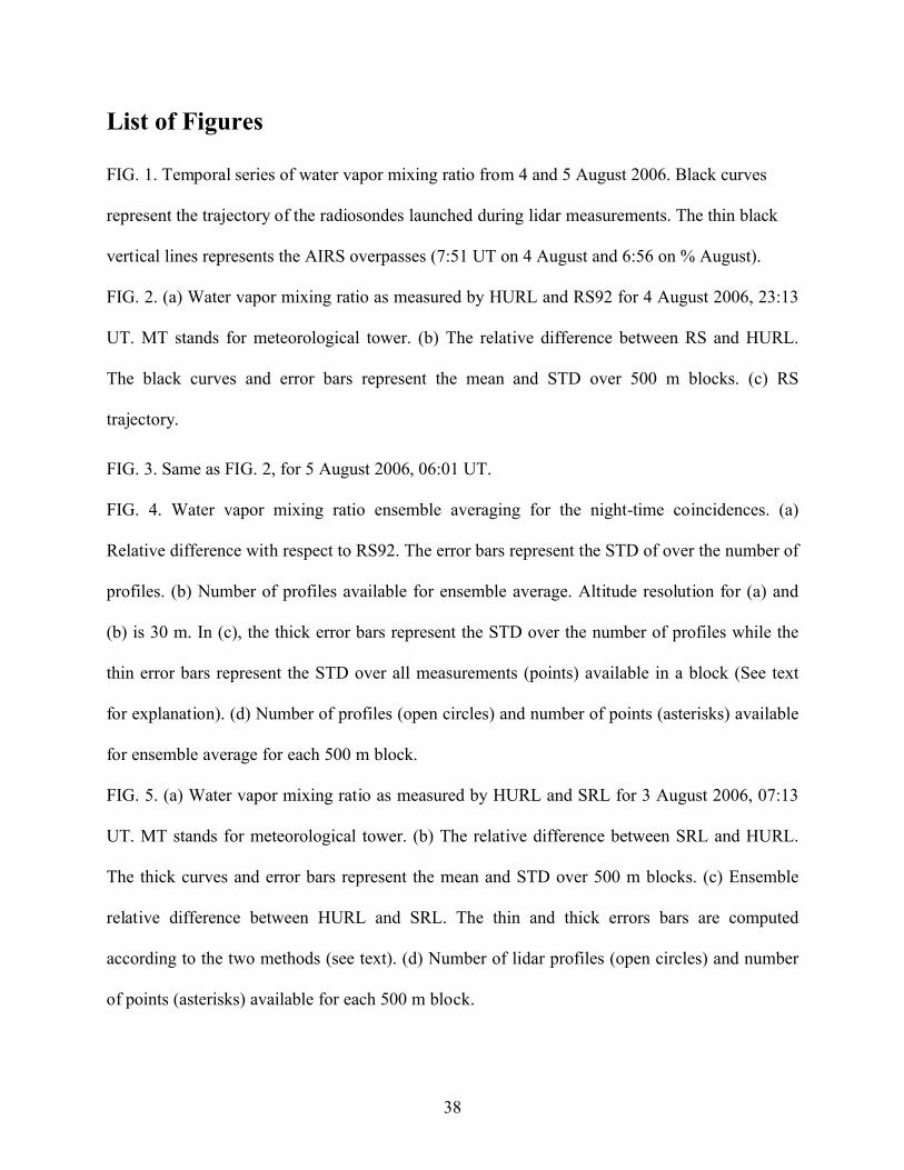
List of Figures

FIG. 1. Temporal series of water vapor mixing ratio from 4 and 5 August 2006. Black curves

represent the trajectory of the radiosondes launched during lidar measurements. The thin black

vertical lines represents the AIRS overpasses (7:51 UT on 4 August and 6:56 on % August).

FIG. 2. (a) Water vapor mixing ratio as measured by HURL and RS92 for 4 August 2006, 23:13

UT. MT stands for meteorological tower. (b) The relative difference between RS and HURL.

The black curves and error bars represent the mean and STD over 500 m blocks. (c) RS

trajectory.

FIG. 3. Same as FIG. 2, for 5 August 2006, 06:01 UT.

FIG. 4. Water vapor mixing ratio ensemble averaging for the night-time coincidences. (a)

Relative difference with respect to RS92. The error bars represent the STD of over the number of

profiles. (b) Number of profiles available for ensemble average. Altitude resolution for (a) and

(b) is 30 m. In (c), the thick error bars represent the STD over the number of profiles while the

thin error bars represent the STD over all measurements (points) available in a block (See text

for explanation). (d) Number of profiles (open circles) and number of points (asterisks) available

for ensemble average for each 500 m block.

FIG. 5. (a) Water vapor mixing ratio as measured by HURL and SRL for 3 August 2006, 07:13

UT. MT stands for meteorological tower. (b) The relative difference between SRL and HURL.

The thick curves and error bars represent the mean and STD over 500 m blocks. (c) Ensemble

relative difference between HURL and SRL. The thin and thick errors bars are computed

according to the two methods (see text). (d) Number of lidar profiles (open circles) and number

of points (asterisks) available for each 500 m block.

39

FIG. 6. Water vapor mixing ratio as measured by HURL and NWS Sippican Mark IIA on 27

July 2006, 3:36 UT. (a)-(b) Temperature and relative humidity during RS flight. (c) WVMR; MT

stands for meteorological tower. (d) Relative difference with respect to RS. The Thick curve

represents the mean profiles over 500 m blocks.

FIG. 7. Same as FIG.. 6, for 5 August 2006, 3:30 UT.

FIG. 8. (a) Relative difference with respect to Mark IIA. The thick error bars represent the STD

over the number of profiles while the thin error bars represent the STD over all measurements

(points) available in a block. See text for explanation. (b) Number of lidar profiles (open circles)

and number of points (asterisks) available for each 500 m block.

FIG. 9. HURL – Mark IIA RS grid comparison for 27 July 2006, 3:36 UT. (a) Number of events

for each grid-box, characterized by ΔT = 10 °C and ΔRH = 10 %. (b) RMS [%] for each grid-

box. The largest RMS occurs over the region characterized by T = [-30, -20] °C and RH = [10,

20] %.

FIG. 10. HURL – Mark IIA RS grid comparison for 5 August 2006, 3:30 UT. (a) Number of

events for each grid-box, characterized by ΔT = 10 °C and ΔRH = 10 %. (b) RMS [%] for each

box. The largest RMS occurs over the region characterized by T = [0, 10] °C and RH = [10, 20]

%.

FIG. 11. HURL – Mark IIA RS grid comparison for the ensemble averaging over all 15

comparisons. (a) Number of events for each grid-box, characterized by ΔT = 10 °C and ΔRH =

10 %. (b) RMS [%] for each grid-box. The largest RMS occurs over the region with T = [-30, -20]

°C and RH = [10, 20] % (RMS = 95 %). Relatively large RMS can be observed over regions with

T = [-30, -20] °C and RH = [20, 30] % (RMS =62.4 %) and other regions with T = [-30, -20] °C

and RH = [20, 70] % or T = [-20, 20] °C and RH = [10, 20] %.

40

FIG. 12. (a) – (c) HURL-AIRS water vapor mixing ratio for 4 August 2006 (Aqua overpass

07:51 UT) and 5 August 2006 (Aqua overpass 06:56 UT). The HURL profiles are shown at both

original resolution and averaged over 2 km layers. (b) – (d) Relative difference with respect to

HURL within 2 km layers.

FIG. 13. (a) HURL-TES water vapor mixing ratio for 11 July 2006, Aura overpass 07:15 UT. (b)

Relative difference with respect to HURL after applying a priori profile and kernels. (c) HURL-

TES-CFH-RS92 water vapor mixing ratio for 12 August 2006, Aura overpass 07:16 UT. (d)

Relative difference with respect to HURL, CFH and RS92 after applying a priori profile and

kernels. X stands for HURL, CFH or RS92.

41

FIG. 1. Temporal series of water vapor mixing ratio from 4 and 5 August 2006. Black curves represent the trajectory of the radiosondes launched during lidar measurements. The thin black vertical lines represents the AIRS overpasses (7:51 UT on 4 August and 6:56 on % August).

42

FIG. 2. (a) Water vapor mixing ratio as measured by HURL and RS92 for 4 August 2006, 23:13 UT. MT stands for meteorological tower. (b) The relative difference between RS and HURL. The black curves and error bars represent the mean and STD over 500 m blocks. (c) RS trajectory.

43

FIG. 3. Same as FIG. 2, for 5 August 2006, 06:01 UT.

44

FIG. 4. Water vapor mixing ratio ensemble averaging for the night-time coincidences. (a) Relative difference with respect to RS92. The error bars represent the STD of over the number of profiles. (b) Number of profiles available for ensemble average. Altitude resolution for (a) and (b) is 30 m. In (c), the thick error bars represent the STD over the number of profiles while the thin error bars represent the STD over all measurements (points) available in a block (See text for explanation). (d) Number of profiles (open circles) and number of points (asterisks) available for ensemble average for each 500 m block.

45

FIG. 5. (a) Water vapor mixing ratio as measured by HURL and SRL for 3 August 2006, 07:13 UT. MT stands for meteorological tower. (b) The relative difference between SRL and HURL. The thick curves and error bars represent the mean and STD over 500 m blocks. (c) Ensemble relative difference between HURL and SRL. The thin and thick errors bars are computed according to the two methods (see text). (d) Number of lidar profiles (open circles) and number of points (asterisks) available for each 500 m block.

46

FIG. 6. Water vapor mixing ratio as measured by HURL and NWS Sippican Mark IIA on 27 July 2006, 3:36 UT. (a)-(b) Temperature and relative humidity during RS flight. (c) WVMR; MT stands for meteorological tower. (d) Relative difference with respect to RS. The Thick curve represents the mean profiles over 500 m blocks.

47

FIG. 7. Same as FIG. 6, for 5 August 2006, 3:30 UT.

48

FIG. 8. (a) Relative difference with respect to Mark IIA. The thick error bars represent the STD over the number of profiles while the thin error bars represent the STD over all measurements (points) available in a block. See text for explanation. (b) Number of lidar profiles (open circles) and number of points (asterisks) available for each 500 m block.

49

FIG. 9. HURL – Mark IIA RS grid comparison for 27 July 2006, 3:36 UT. (a) Number of events for each grid-box, characterized by ΔT = 10 °C and ΔRH = 10 %. (b) RMS [%] for each grid-box. The largest RMS occurs over the region characterized by T = [-30, -20] °C and RH = [10, 20] %.

50

FIG. 10. HURL – Mark IIA RS grid comparison for 5 August 2006, 3:30 UT. (a) Number of events for each grid-box, characterized by ΔT = 10 °C and ΔRH = 10 %. (b) RMS [%] for each box. The largest RMS occurs over the region characterized by T = [0, 10] °C and RH = [10, 20] %.

51

FIG. 11. HURL – Mark IIA RS grid comparison for the ensemble averaging over all 15 comparisons. (a) Number of events for each grid-box, characterized by ΔT = 10 °C and ΔRH = 10 %. (b) RMS [%] for each grid-box. The largest RMS occurs over the region with T = [-30, -20] °C and RH = [10, 20] % (RMS = 95 %). Relatively large RMS can be observed over regions with T = [-30, -20] °C and RH = [20, 30] % (RMS =62.4 %) and other regions with T = [-30, -20] °C and RH = [20, 70] % or T = [-20, 20] °C and RH = [10, 20] %.

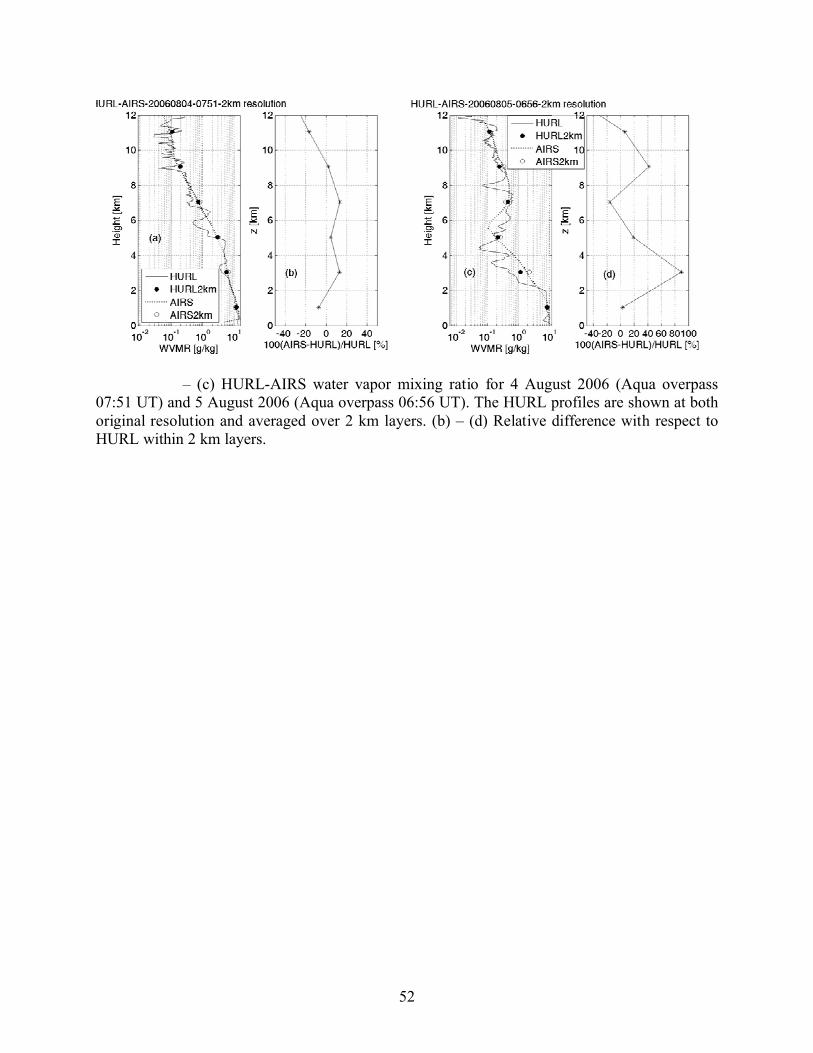
52

FIG. 12. (a) – (c) HURL-AIRS water vapor mixing ratio for 4 August 2006 (Aqua overpass 07:51 UT) and 5 August 2006 (Aqua overpass 06:56 UT). The HURL profiles are shown at both original resolution and averaged over 2 km layers. (b) – (d) Relative difference with respect to HURL within 2 km layers.

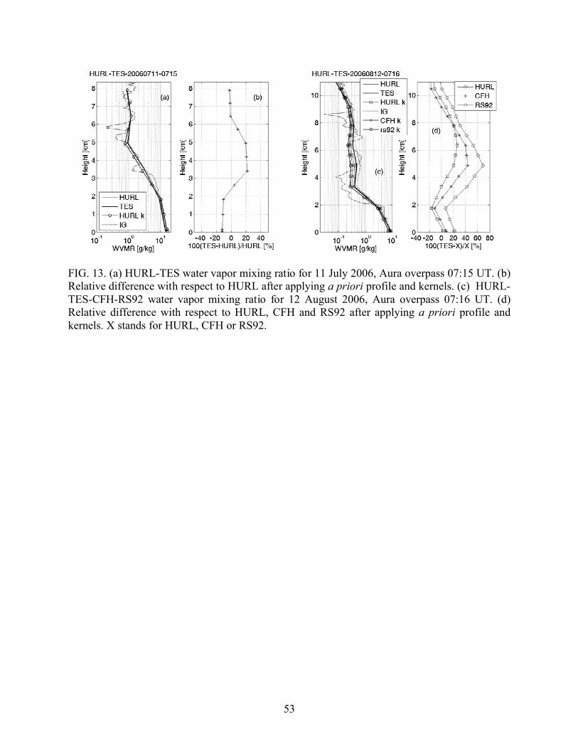
53

FIG. 13. (a) HURL-TES water vapor mixing ratio for 11 July 2006, Aura overpass 07:15 UT. (b) Relative difference with respect to HURL after applying a priori profile and kernels. (c) HURL-TES-CFH-RS92 water vapor mixing ratio for 12 August 2006, Aura overpass 07:16 UT. (d) Relative difference with respect to HURL, CFH and RS92 after applying a priori profile and kernels. X stands for HURL, CFH or RS92.