Water Resources Research Report - Western Engineering · 2017-07-24 · Coastal cities are particularly threatened by hydro-meteorological climate hazards including: hurricanes, tsunamis,

THE UNIVERSITY OF WESTERN ONTARIO

DEPARTMENT OF CIVIL AND

ENVIRONMENTAL ENGINEERING

Water Resources Research Report

Report No: 083

Date: April 2013

Coastal Cities at Risk (CCaR): Generic System

Dynamics Simulation Models for Use with City

Resilience Simulator

FINAL REPORT

By:

Angela Peck

and

Slobodan P. Simonovic

ISSN: (print) 1913-3200; (online) 1913-3219;

ISBN: (print) 978-0-7714-XXXX-X; (online) 978-0-7714-XXXX-X;

i

Coastal Cities at Risk (CCaR): Generic System Dynamics Simulation Models

for Use with City Resilience Simulator

Angela Peck

Slobodan P. Simonovic

Department of Civil and Environmental Engineering

The University of Western Ontario

London, Ontario, Canada

April 2013

ii

EXECUTIVE SUMMARY

It is projected that 67% of global population will be living in urban areas by 2050; an increase of

approximately 30% from global urban population in 2011 (United Nations 2012). This

anticipated increase may be attributed to the trend of increasing rural-to-urban migration as

people abandon agricultural practices to seek out economic opportunities and prosperity in urban

cities (Akanda and Hossain 2012; Wenzel et al. 2007). Migration is causing many major cities to

rapidly grow into megacities (Akanda and Hossain 2012; United Nations 2008); defined by the

United Nations (2008; 2012) as cities with populations greater than 10 million people. A

majority of the world’s current and projected megacities are located in hazardous low-lying

coastal areas, particularly in the developing world. Therefore, millions of people are exposed to

coastal climate hazards. In addition, the megacities are often characterized by high population

densities, destitute slum settlements and inadequate life-sustaining infrastructure (Wenzel et al.

2007); conditions which exacerbate the impacts of climate hazards.

Coastal cities are particularly threatened by hydro-meteorological climate hazards including:

hurricanes, tsunamis, storms, storm surges, flooding and sea-level rise. The climate is changing

and so are the spatial and temporal patterns and characteristics (frequency, magnitude, intensity

and seasonality) of climate hazards (IPCC 2012). Many coastal cities are already experiencing

the consequences of a changing climate and many more can expect an increased frequency of

high magnitude events in the future (IPCC 2012). Climate hazards have dynamic and complex

impacts on environmental and human systems; which often result in natural disasters. With close

to 10% of the global population living in low-elevation coastal zones, there is an increased

necessity for estimating and reducing the impacts of coastal disasters (United Nations 2011).

Climate change caused hazards will continue to have a significant impact on coastal cities in the

future. Therefore, effective adaptation to natural disasters is an essential component of a

comprehensive, long-term disaster management strategy.

The work presented in this report is part of an international project "Coastal Cities at Risk:

Building Adaptive Capacity for Managing Climate Change in Coastal Megacities" supported by

the International Research Initiative on Adaptation to Climate Change of the Canadian

iii

International Development Research Centre (IDRC). This report focuses on a system dynamics

simulation (SD) approach for understanding the behaviour of complex city systems to climate

change caused natural disasters. This approach captures the dynamic characteristics of disaster

impacts. A quantitative resilience measure is used to assess a city’s capacity to manage climate

change disasters. Simulation of resilience in time and space allows for the assessment and

comparison of alternative adaptation measures. The project involves a methodology for assessing

the impacts of hydro-meteorological disasters on four coastal megacities across the globe:

Vancouver in Canada, Lagos in Nigeria, Manila in Philippines and Bangkok in Thailand.

The objectives of this report are to: (i) present an original systems framework for quantifying

resilience and introduce a space-time dynamic resilience measure (ST-DRM); (ii) discuss ST-

DRM theory and calculations; (iii) introduce Generic System Dynamics Simulation Models

(GSDSMs) and provide implementation example; (iv) present a high-level structure of the City

Resilience Simulator (CRS); and (v) provide current state of modeling progress for the CCaR

project and outline future work.

The report is organized as follows: Chapter 1 introduces the research topic and provides some

background information on the CCaR project; Chapter 2 gives more technical and theoretical

details pertaining to the development of a City Resilience Simulator (CRS); Chapter 3 provides a

description of the Generic System Dynamics Simulation Models (GSDSMs); Chapter 4 provides

a detailed description of how to use the GSDSMs to develop unique CRSs for the CCaR project

partner coastal cities; Chapter 5 presents a GSDSM implementation example; and finally,

Chapter 6 provides a summary of work presented and anticipated future work.

iv

TABLE OF CONTENTS

EXECUTIVE SUMMARY .......................................................................................................................... ii

LIST OF TABLES ....................................................................................................................................... vi

LIST OF FIGURES ..................................................................................................................................... vi

LIST OF ACRONYMS .............................................................................................................................. vii

1. INTRODUCTION ................................................................................................................................ 1

1.1 Impacts (i) ........................................................................................................................................... 2

1.1.1 Physical Impacts .......................................................................................................................... 2

1.1.2 Economic Impacts ........................................................................................................................ 3

1.1.3 Social Impacts .............................................................................................................................. 4

1.1.4 Health Impacts ............................................................................................................................. 4

1.1.5 Organizational Impacts ................................................................................................................ 5

1.2 Adaptive Capacity (AC) ...................................................................................................................... 5

1.2.1 Properties of Adaptive Capacity (Ri) ........................................................................................... 5

1.3 Integration of Impacts ......................................................................................................................... 6

2. RESILIENCE ........................................................................................................................................ 7

2.1 Introduction ......................................................................................................................................... 8

2.2 Resilience Quantification .................................................................................................................... 9

2.2.1 Dimensions of Resilience ........................................................................................................... 10

2.2.2 Impacts and Capacities............................................................................................................... 10

2.2.3 Resilience Sectors ...................................................................................................................... 13

3. GENERIC SYSTEM DYNAMICS SIMULATION MODELS (GSDSMs) ...................................... 14

3.1 GSDSMs: Description ...................................................................................................................... 15

3.2 GSDSMs: Use ................................................................................................................................... 23

4. CITY RESILIENCE SIMULATOR (CRS) ........................................................................................ 30

5. CONCLUSIONS ................................................................................................................................. 33

ACKNOWLEDGEMENTS ........................................................................................................................ 34

v

REFERENCES ........................................................................................................................................... 34

APPENDIX A: Description of variables in the H1_Hospital example ....................................................... 37

APPENDIX B: Description of the Distribution Package ............................................................................ 41

APPENDIX C: List of Previous Reports in the Series ............................................................................... 43

vi

LIST OF TABLES

Table 1: Resilience characteristics of critical lifeline services based on the four R’s; adapted from

Bruneau et al. (2003)

Table 2: Vensim simulation model settings

Table 3: Suggested steps for successful implementation of GSDSMs

Table 4: GSDSM-H health example

LIST OF FIGURES

Figure 1: Causal loop diagram of city resilience measure

Figure 2: Illustration of system performance subject to a disturbance

Figure 3: Illustration of system resilience in system performance space

Figure 4: System resilience

Figure 5: Opening the library of GSDSMs

Figure 6: GSDSM-E; economic generic model structure

Figure 7: GSDSM-H; health generic model structure

Figure 8: GSDSM-O; organizational generic model structure

Figure 9: GSDSM-P; physical generic model structure

Figure 10: GSDSM-S; social generic model structure

Figure 11: The output of the various GSDSM-5 models; could continue expanding to

accommodate any number of GSDSMs

Figure 12: GSDSM-C generic form in Vensim; add as many H, S, E, O, and P variables as

necessary

vii

Figure 13: GSDSM-C in Vensim; an illustrative example

Figure 14: GSDSM-C model settings in Vensim; an illustrative example

Figure 15: GSDSM-C simulation results for overall city resilience measure; an illustrative

example

Figure 16: GSDSM-C simulation results for overall city resilience measure; an illustrative

example

Figure 17: GSDSM-H H1_Hospital example

Figure 18: GSDSM-H hospital example; save as a new file name (e.g. H1_Hospital)

Figure 19: H1_Hospital example; simulation model structure

Figure 20: H1_Hospital example; model settings

Figure 21: H1_Hospital example; injured patients

Figure 22: H1_Hospital example; H1 resilience

Figure 23: A conceptual diagram of the CRS structure

Figure 24: An example of short term model settings

Figure 25: An example of long term model settings

LIST OF ACRONYMS

AC Adaptive Capacity

CCaR Coastal Cities at Risk

CIHR Canadian Institute of Health Research

CRS City Resilience Simulator

CRS-N-L City Resilience Simulator for long duration, continuous hazards

CRS-N-S City Resilience Simulator for short duration, event-based hazards

CRS-B City Resilience Simulator for Bangkok, Thailand

CRS-L City Resilience Simulator for Lagos, Nigeria

viii

CRS-M City Resilience Simulator for Manila, Philippines

CRS-V City Resilience Simulator for Vancouver, Canada

GSDSMs Generic System Dynamics Simulation Models

GSDSM-C Generic System Dynamics Simulation Model – Combined

GSDSM-E Generic System Dynamics Simulation Model – Economic

GSDSM-H Generic System Dynamics Simulation Model – Health

GSDSM-O Generic System Dynamics Simulation Model – Organizational

GSDSM-P Generic System Dynamics Simulation Model – Physical

GSDSM-S Generic System Dynamics Simulation Model – Social

GIS Geographic Information System

IDRC International Development Research Centre

IRIACC International Research Initiative on Adaptation to Climate Change

NSERC Natural Sciences and Engineering Research Council of Canada

OBD Overall Burden Disease

SD System Dynamics

SDRM Single Dynamic Resilience Measure

SSHRC Social Sciences and Humanities Research Council of Canada

ST-DRM Space-Time Dynamic Resilience Measure

1

1. INTRODUCTION

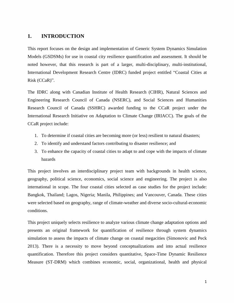
This report focuses on the design and implementation of Generic System Dynamics Simulation

Models (GSDSMs) for use in coastal city resilience quantification and assessment. It should be

noted however, that this research is part of a larger, multi-disciplinary, multi-institutional,

International Development Research Centre (IDRC) funded project entitled “Coastal Cities at

Risk (CCaR)”.

The IDRC along with Canadian Institute of Health Research (CIHR), Natural Sciences and

Engineering Research Council of Canada (NSERC), and Social Sciences and Humanities

Research Council of Canada (SSHRC) awarded funding to the CCaR project under the

International Research Initiative on Adaptation to Climate Change (IRIACC). The goals of the

CCaR project include:

1. To determine if coastal cities are becoming more (or less) resilient to natural disasters;

2. To identify and understand factors contributing to disaster resilience; and

3. To enhance the capacity of coastal cities to adapt to and cope with the impacts of climate

hazards

This project involves an interdisciplinary project team with backgrounds in health science,

geography, political science, economics, social science and engineering. The project is also

international in scope. The four coastal cities selected as case studies for the project include:

Bangkok, Thailand; Lagos, Nigeria; Manila, Philippines; and Vancouver, Canada. These cities

were selected based on geography, range of climate-weather and diverse socio-cultural-economic

conditions.

This project uniquely selects resilience to analyze various climate change adaptation options and

presents an original framework for quantification of resilience through system dynamics

simulation to assess the impacts of climate change on coastal megacities (Simonovic and Peck

2013). There is a necessity to move beyond conceptualizations and into actual resilience

quantification. Therefore this project considers quantitative, Space-Time Dynamic Resilience

Measure (ST-DRM) which combines economic, social, organizational, health and physical

2

impacts of climate change caused natural disasters on coastal megacities. The theoretical

background of the ST-DRM is included in Chapter 2 of the report.

1.1 Impacts (i)

The five major impacts that are being considered in the ST-DRM calculation include: economic

impacts, health impacts, physical impacts, organizational impacts and social impacts (Simonovic

and Peck 2013). These impacts require the modification of GSDSMs for the four city models to

properly describe the local conditions in each city.

1.1.1 Physical Impacts

Coastal cities are exposed to multiple types of hydro-meteorological climate hazards including:

storm surges, tsunamis, sea-level rise, hurricanes, and coastal and riverine flooding. These

hazards drive the physical sector of the CRS that represents the natural sub-system. Climate

change and urbanization will exacerbate the problems associated with these hazards in urban

coastal megacities as the frequency and magnitude of events increases. These changes in the

physical system have direct and indirect impacts on economic, social, health and organizational

activities.

Hazards are described by climatological variables in the physical sector of the CRS. The physical

impacts sector is connected to other sectors in the CRS which affect resilience (Figure 1). For

instance, consider the flood hazard. Riverine flooding directly affects water quality, which in

turn may affect the health of a population and therefore impact the economy. Some areas within

a city may experience larger impacts than others based on the magnitude of hazard (ex. depth of

flooding), pre-disaster demographic and economic characteristics and social inequities.

3

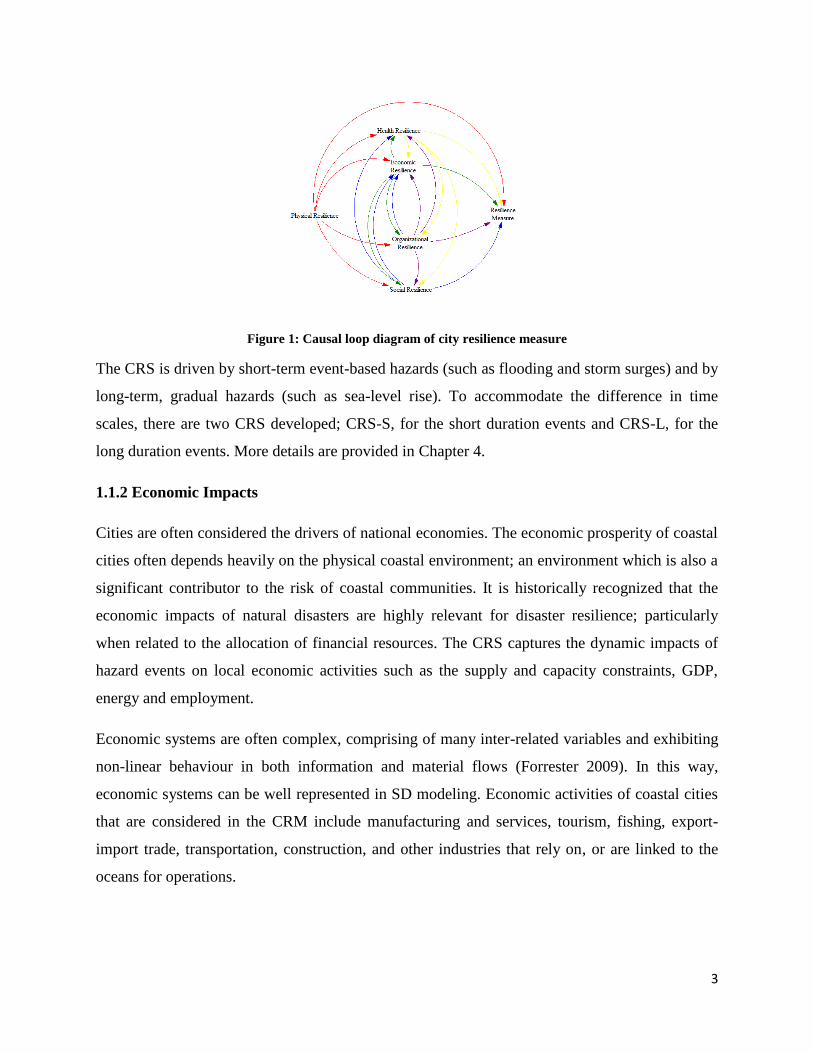
Figure 1: Causal loop diagram of city resilience measure

The CRS is driven by short-term event-based hazards (such as flooding and storm surges) and by

long-term, gradual hazards (such as sea-level rise). To accommodate the difference in time

scales, there are two CRS developed; CRS-S, for the short duration events and CRS-L, for the

long duration events. More details are provided in Chapter 4.

1.1.2 Economic Impacts

Cities are often considered the drivers of national economies. The economic prosperity of coastal

cities often depends heavily on the physical coastal environment; an environment which is also a

significant contributor to the risk of coastal communities. It is historically recognized that the

economic impacts of natural disasters are highly relevant for disaster resilience; particularly

when related to the allocation of financial resources. The CRS captures the dynamic impacts of

hazard events on local economic activities such as the supply and capacity constraints, GDP,

energy and employment.

Economic systems are often complex, comprising of many inter-related variables and exhibiting

non-linear behaviour in both information and material flows (Forrester 2009). In this way,

economic systems can be well represented in SD modeling. Economic activities of coastal cities

that are considered in the CRM include manufacturing and services, tourism, fishing, export-

import trade, transportation, construction, and other industries that rely on, or are linked to the

oceans for operations.

4

1.1.3 Social Impacts

In affluent communities, people find it desirable to live close to the coast. In poorer communities

however, people who have been displaced, or rely on close proximity to water for survival, live

closest to the water, which makes them particularly susceptible to impacts of climate caused

hydro-meteorological hazards. The relationship between poverty, environmental degradation and

hazard vulnerability is a vicious, mutually reinforcing system of feedbacks (Kesavan 2006)

especially prevalent in developing countries. The potential impacts of natural disasters on social

systems may be very severe.

1.1.4 Health Impacts

Climate related natural hazards can have significant health impacts on a population. Hazards may

trigger outbreaks of disease (Paton and Johnson 2006) and hazard debris can cause injury, which

may immediately impede mobility and hinder evacuation and response efforts. Hydro-

meteorological hazards such as floods, tsunamis and storm surges also carry waste, sewage and

bacteria which, through direct contact with drinking water supplies, could spread disease and

cause illness for many weeks beyond the duration of a disaster. It is also possible that illness and

disease may be spread without direct contact with hazard phenomena through the close

proximity of infected people in confined areas. It is therefore important to estimate and anticipate

potential health impacts to better prepare for, respond to and recover from climate caused natural

disasters.

The present study considers a composite health index to quantify the health effects of climate

hazards in coastal cities (Owrangi et al. 2012). This index is used as part of the CRM and

considers Disability Adjusted Life Years (DALYs) as a measure of Overall Burden of Disease

(OBD) within a city. This time-dependent measure, originally developed for the World Health

Organization and World Bank in the 1990s, is used to capture the health vulnerability of a

population in the CRM. DALYs are based on health factors that are considered to contribute to

premature death; the number of cases of injuries, communicable and non-communicable diseases

that are prevalent in a country for a particular year. In the CRS, changes in DALY values reflect

the health impacts of natural disasters directly through physical-health sector links and indirectly

through economic and social links.

5

However, there are temporal challenges in using the DALY approach to represent human health

in the CRS. For instance, it becomes difficult to accurately assess OBD consequences due to a

specific hazard event due to the diverse time scales required to diagnose various health impacts.

For instance, injuries often occur immediately during a disaster event, whereas some illnesses

and diseases do not display symptoms for weeks, and some may not show any symptoms at all.

These afflictions may be left undiagnosed or untreated for years following the initial disaster.

Thus, there are difficulties directly linking long-term diseases to a specific hazard event

especially considering the potential influences of external environmental factors during a

disease’s incubation time.

1.1.5 Organizational Impacts

The effectiveness of climate change adaptation measures must consider the political

administrative and institutional framework which affects the functioning of the coastal megacity.

This framework defines the overall effectiveness of decision making. It must be framed because

the overall implementation and effectiveness of climate change adaptation options depends on

political motivation, budgets and climate change policy. The manner in which a city formulates

policy decisions is not explicitly represented in the CMRS model structure but it is incorporated

as an essential part of adaptation scenarios to be simulated by the model.

1.2 Adaptive Capacity (AC)

The impacts of a disaster exhibit temporal and spatial variability that are caused direct

interactions between impacts of a disaster (social, health, economic, and other) and adaptive

capacity of the urban system to absorb them. Adaptive capacity is defined using various

performance measures. These measures are defined, in terms of four R's (robustness,

redundancy, resourcefulness and rapidity).

1.2.1 Properties of Adaptive Capacity (Ri)

The proposed method of resilience quantification (presented in details in Chapter 2 of this report)

is based, in part, on the four properties ( of adaptive capacity (AC) as identified by Bruneau et

al (2003) and adapted by Simonovic and Peck (2013). The adaptive capacity of physical and

social systems can be defined using:

6

i. Robustness ( ): strength and the ability of elements or systems to resist stress without

suffering damages or loss of function;

ii. Redundancy ( ): the extent to which elements or systems satisfy functional

requirements in the event of disruptions, disturbances, or damages;

iii. Resourcefulness ( ): the capacity to identify problems, establish priorities and mobilize

financial and human resources to elements or systems that are threatened by disruption,

disturbance, or damage; and

iv. Rapidity ( ): the capacity to meet priorities and achieve goals in a timely manner to

contain losses, minimize damages and avoid future disruptions.

The as a function of time and space may therefore be expressed as follows:

( [ ( ] (1)

These 4R’s of AC will be quantified in the CRS by measuring performance of indicators. These

indicators of AC will be selected in conjunction with experts and through rigorous research

efforts. The remainder of this report discusses AC in terms of the 4R properties and indicators in

the temporal context only. The resilience model framework has not yet incorporated any spatial

dimension into its calculations. Both space-time dimensions are presented in the expressions of

resilience, impacts and adaptive capacity to present the comprehensive description, because

incorporating the spatial dimension is a part of plans for future work.

1.3 Integration of Impacts

In existing and emerging megacities, the relationship between health, economy, society, and the

environment is more complex than ever (Akanda and Hossain 2012). Seemingly unrelated

elements may influence each other indirectly through links with other system elements. To

capture these dynamic system interactions, this research considers use of a system dynamics

simulation tool, called a City Resilience Simulator (CRS). The CRS is intended to determine city

resilience in response to a disaster and the ability of the urban system to react, cope and adapt to

disaster impacts. The CRS is comprised of multiple systems linked together used to compute the

value of the ST-DRM. The CRS framework is introduced in Chapter 4.

7

2. RESILIENCE

The most common approach to urban disaster management is focused on the assessment of

vulnerability, which when combined with hazards, provides for disaster risk evaluation.

Vulnerability describes the pre-event, inherent characteristics or qualities of urban systems that

create the potential for harm. Vulnerability is a function of whom or what is at risk and

sensitivity of system (the degree to which people and places can be harmed). On the other side,

resilience is the ability of a complex system to respond and recover from disasters and includes

those conditions that allow the system to absorb impacts and cope with an event, as well as post-

event, adaptive processes that facilitate the ability of the system to re-organize, change, and learn

in response to a threat (Simonovic and Peck 2013). Drawing from resilience literature in the

fields of physics, ecology and hazards, some common elements in the definition of resilience

include: (i) minimization of losses, damages and community disruption; (ii) maximization of the

ability and capacity to adapt and adjust when there are shocks to systems; (iii) returning systems

to a functioning state as quickly as possible; (iv) recognition that resilient systems are dynamic in

time and space; and (v) acknowledgements that post-shock functioning levels may not be the

same as pre-shock levels.

The theory behind developing a CRS is built on a the fundamental concept that a resilient city is

a sustainable network of physical (constructed and natural) systems and human communities

(social and institutional) that possess the capacity to survive, cope, recover, learn and transform

from disturbances by: (i) reducing failure probabilities; (ii) reducing consequences; (iii) reducing

time to recovery; and (iv) creating opportunity for development and innovation from adverse

impacts.

To deal with the shortcomings in existing resilience models and to provide a conceptual basis for

establishing baselines for measuring resilience, this project introduces a space-time dynamic

resilience measure (ST-DRM). A CRS will capture the process of dynamic disaster resilience

simulation in both, time and space.

8

2.1 Introduction

In this research, a systems dynamics simulation (SD) approach is selected to understand the

behaviour of complex city systems subject to climate change caused disasters. This approach was

selected in order to capture the dynamic characteristics of disaster impacts and disaster resilience

behaviour of coastal megacities. The remainder of this chapter will describe the basic concepts

behind the development of a CRS and provide the theoretical basis and the vocabulary used in

this report to define disaster resilience. This chapter: (a) introduces a method for quantifying

disaster resilience; (b) defines disaster resilience as dynamic in both time and space; and (c)

presents resilience as framework for integration of impacts (physical, operational, social,

technological, economic and health).

The ST-DRM is defining the level of system performance in time ( and a particular location in

space ( (Simonovic and Peck 2013). The measure integrates various units ( that characterize

impacts of disasters on urban community. At the current level of development the following

units of resilience ( are considered: physical, health, economic, social and organizational.

Measures of performance for physical impacts ( ( ) may include length [km] of road

being inundated by a flood, or the reduction in water supply [m3/s] due to pipe break, or the area

of the city [km2] that is under the water during a flood event, or the height of the sea wall [m] that

provides the coastal protection, and so on. The health impacts ( ( may be measured

using an integral index like disability adjusted life year (DALY), or the number of hospital beds

in emergency hospitals, or the number of doctors per capita, and so on. The economic

( ( ) impacts can be measured using aggregates like GDP, or much more

sophisticated expressions of production, supply and consumption chains obtained through input-

output modeling. The measure of performance for social impacts ( ( ) can be

expressed using indicators like age, gender, ethnicity, social status, education and household

arrangement. The organizational impacts ( ( ) can be measured using number of

disaster management services available to the population, or the time [hr] required under the

current regulations to provide assistance or process a damage claim, or similar. This approach is

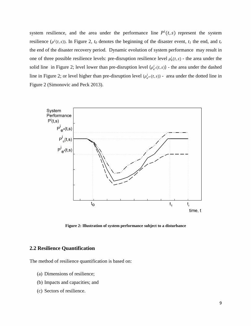
based on the notion that an impact, ( , which varies with time and location in space, has

been defined for the quality of the resilience component of a community, see Figure 2. The area

between the initial performance line ( and performance line ( represents the loss of

9

system resilience, and the area under the performance line ( represent the system

resilience ( ( ). In Figure 2, t0 denotes the beginning of the disaster event, t1 the end, and tr

the end of the disaster recovery period. Dynamic evolution of system performance may result in

one of three possible resilience levels: pre-disruption resilience level ( - the area under the

solid line in Figure 2; level lower than pre-disruption level ( ( ) - the area under the dashed

line in Figure 2; or level higher than pre-disruption level ( ( ) - area under the dotted line in

Figure 2 (Simonovic and Peck 2013).

Figure 2: Illustration of system performance subject to a disturbance

2.2 Resilience Quantification

The method of resilience quantification is based on:

(a) Dimensions of resilience;

(b) Impacts and capacities; and

(c) Sectors of resilience.

10

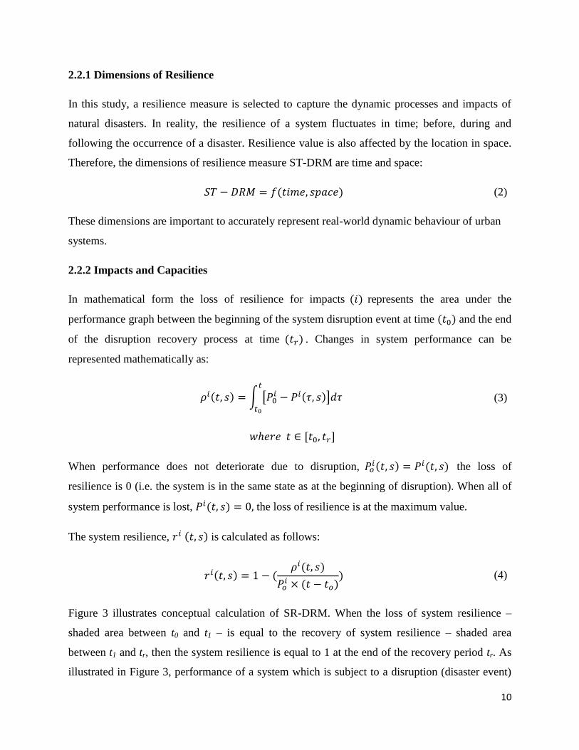
2.2.1 Dimensions of Resilience

In this study, a resilience measure is selected to capture the dynamic processes and impacts of

natural disasters. In reality, the resilience of a system fluctuates in time; before, during and

following the occurrence of a disaster. Resilience value is also affected by the location in space.

Therefore, the dimensions of resilience measure ST-DRM are time and space:

( (2)

These dimensions are important to accurately represent real-world dynamic behaviour of urban

systems.

2.2.2 Impacts and Capacities

In mathematical form the loss of resilience for impacts ( represents the area under the

performance graph between the beginning of the system disruption event at time ( and the end

of the disruption recovery process at time ( . Changes in system performance can be

represented mathematically as:

( ∫ [ ( ]

(3)

When performance does not deteriorate due to disruption, ( ( the loss of

resilience is 0 (i.e. the system is in the same state as at the beginning of disruption). When all of

system performance is lost, ( the loss of resilience is at the maximum value.

The system resilience, ( is calculated as follows:

( ( (

(

(4)

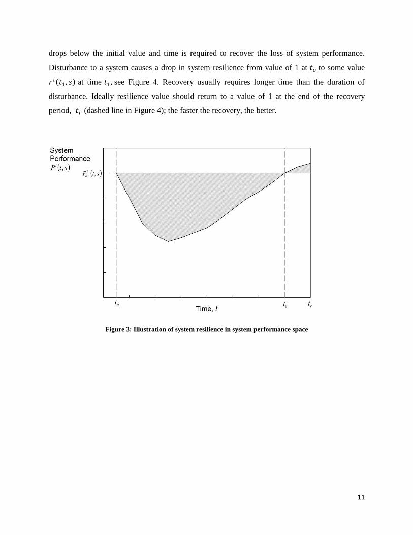
Figure 3 illustrates conceptual calculation of SR-DRM. When the loss of system resilience –

shaded area between t0 and t1 – is equal to the recovery of system resilience – shaded area

between t1 and tr, then the system resilience is equal to 1 at the end of the recovery period tr. As

illustrated in Figure 3, performance of a system which is subject to a disruption (disaster event)

11

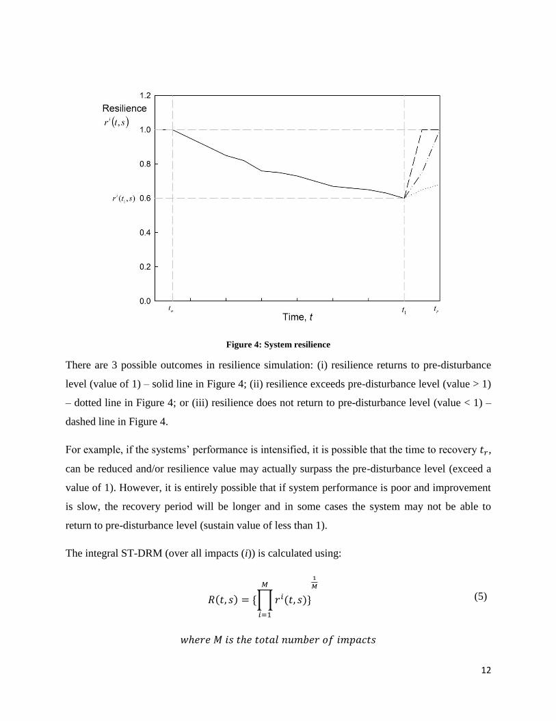
drops below the initial value and time is required to recover the loss of system performance.

Disturbance to a system causes a drop in system resilience from value of 1 at to some value

( at time see Figure 4. Recovery usually requires longer time than the duration of

disturbance. Ideally resilience value should return to a value of 1 at the end of the recovery

period, (dashed line in Figure 4); the faster the recovery, the better.

Figure 3: Illustration of system resilience in system performance space

12

Figure 4: System resilience

There are 3 possible outcomes in resilience simulation: (i) resilience returns to pre-disturbance

level (value of 1) – solid line in Figure 4; (ii) resilience exceeds pre-disturbance level (value > 1)

– dotted line in Figure 4; or (iii) resilience does not return to pre-disturbance level (value < 1) –

dashed line in Figure 4.

For example, if the systems’ performance is intensified, it is possible that the time to recovery ,

can be reduced and/or resilience value may actually surpass the pre-disturbance level (exceed a

value of 1). However, it is entirely possible that if system performance is poor and improvement

is slow, the recovery period will be longer and in some cases the system may not be able to

return to pre-disturbance level (sustain value of less than 1).

The integral ST-DRM (over all impacts (i)) is calculated using:

( ∏ (

(5)

13

Since the calculated value of R(t,s) will change with time and location, the final outcome of the

ST-DRM computation is a dynamic map that shows change of R(t,s) with time and location. In

this report, only time dimension is presented specifically; spatial dimension is still a work in

progress.

2.2.3 Resilience Sectors

The present project introduces an integrated resilience measure that builds on the technical-

organizational-social-economic integration concept by Bruneau et al. (2003) by considering the

resilience measure to be dynamic in both time and space (Simonovic and Peck 2013). The

current project modifies this approach by considering the interactions between physical,

organizational, social, economic, and health components of resilience in order to estimate

disaster impacts and improve disaster resilience (Figure 1).

As an example, improving the capacity of critical lifelines systems during a disaster is important

for developing resilience. Table 1 identifies a selection of these critical lifeline systems and

provides a description in the context of the 4R properties of adaptive capacity. The calculation of

ST-DRM for each impact ( is done at each location ( by solving the following differential

equation:

(

( ( (6)

The ST-DRM integrates resilience types, dimensions and properties by solving for each point in

space (s):

(

( ∏ ( (7)

A generic version of a CRS has been developed by implementing this theoretical framework.

The GSDSMs are the fundamental building blocks used for the construction of a CRS. The

purpose of these generic simulation models is to aid project cities in developing their own CRSs.

A description of the Generic System Dynamics Simulation Models (GSDSMs) and how are they

14

applied is in the following Chapter of the report. However, description is limited to temporal

dimension of impacts, adaptive capacity and resilience as space dimension has not been

incorporated yet.

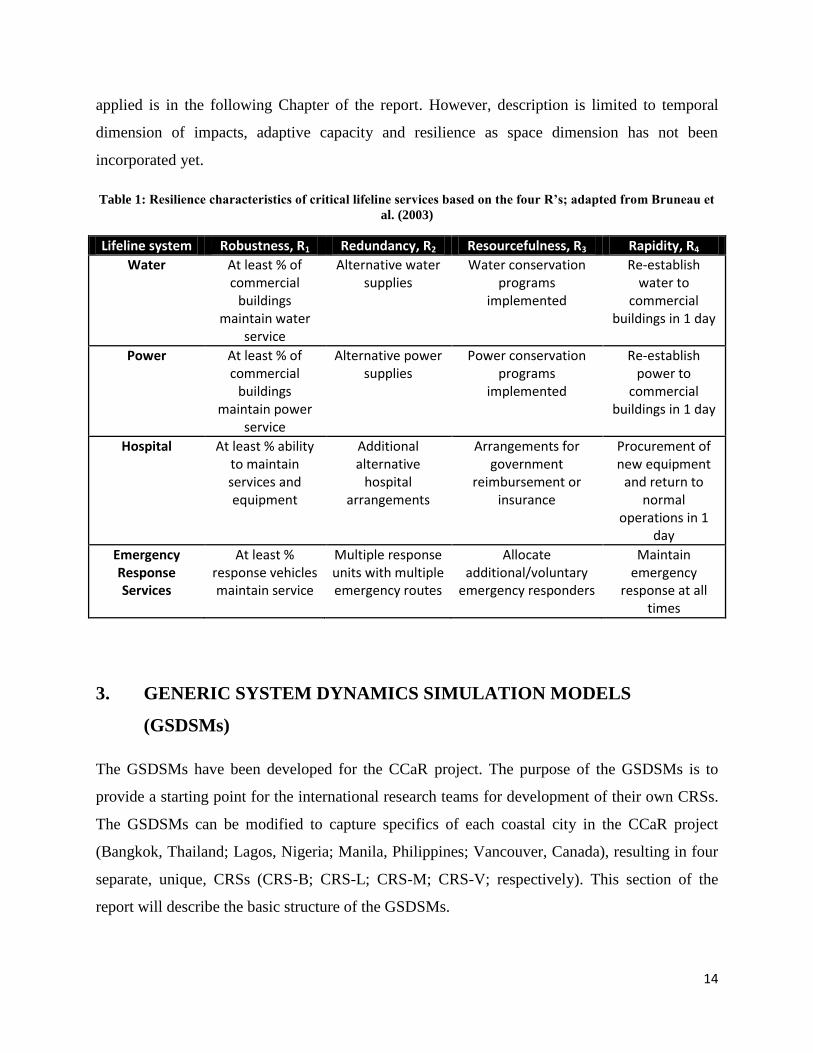
Table 1: Resilience characteristics of critical lifeline services based on the four R’s; adapted from Bruneau et

al. (2003)

Lifeline system Robustness, R1 Redundancy, R2 Resourcefulness, R3 Rapidity, R4

Water At least % of commercial

buildings maintain water

service

Alternative water supplies

Water conservation programs

implemented

Re-establish water to

commercial buildings in 1 day

Power At least % of commercial

buildings maintain power

service

Alternative power supplies

Power conservation programs

implemented

Re-establish power to

commercial buildings in 1 day

Hospital At least % ability to maintain services and equipment

Additional alternative

hospital arrangements

Arrangements for government

reimbursement or insurance

Procurement of new equipment

and return to normal

operations in 1 day

Emergency Response Services

At least % response vehicles maintain service

Multiple response units with multiple emergency routes

Allocate additional/voluntary

emergency responders

Maintain emergency

response at all times

3. GENERIC SYSTEM DYNAMICS SIMULATION MODELS

(GSDSMs)

The GSDSMs have been developed for the CCaR project. The purpose of the GSDSMs is to

provide a starting point for the international research teams for development of their own CRSs.

The GSDSMs can be modified to capture specifics of each coastal city in the CCaR project

(Bangkok, Thailand; Lagos, Nigeria; Manila, Philippines; Vancouver, Canada), resulting in four

separate, unique, CRSs (CRS-B; CRS-L; CRS-M; CRS-V; respectively). This section of the

report will describe the basic structure of the GSDSMs.

15

3.1 GSDSMs: Description

The GSDSMs are a library of generic system dynamics simulation models; six models in total

(Figure 5). Five models were created to represent the five resilience sectors described in Chapter

1, which herein will collectively be referred to as GSDSM-5. The GSDSM-5 corresponds to the

following GSDSMs:

a. GSDSM-E: Economic Simulation Model Figure 6

b. GSDSM-H: Health Simulation Model Figure 7

c. GSDSM-O: Organizational Simulation Model Figure 8

d. GSDSM-P: Physical Simulation Model Figure 9

e. GSDSM-S: Social Simulation Model Figure 10

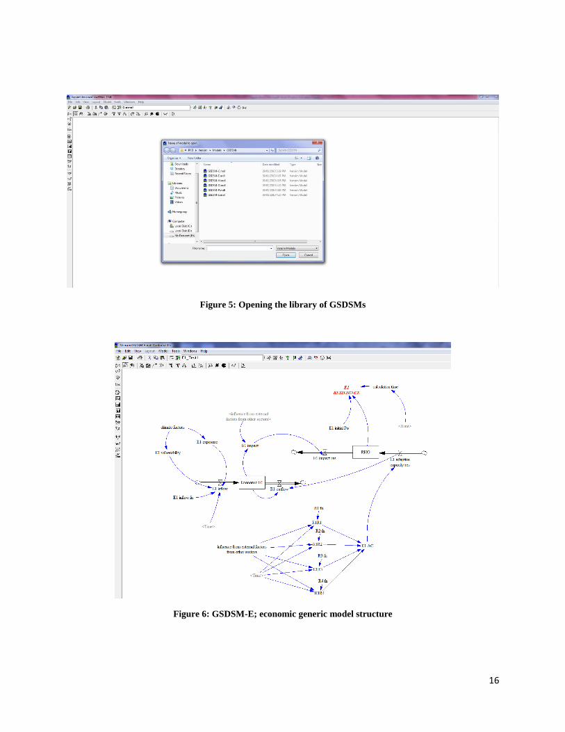
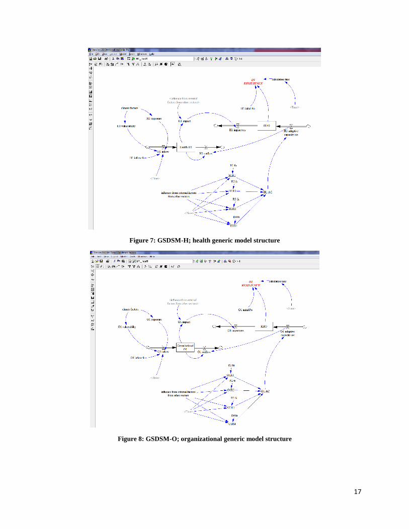
There is actually very little difference between each of the GSDSMs; see Figures 6 – 10. The

only real difference between the GSDSM-5 models is in the name of the system variables; the

system structures are otherwise identical. The reason behind naming the GSDSM-5models

differently is to help categorize systems into one of the 5 resilience sectors. It is important to

keep track of the resilience sector that each system belongs to because when the overall

resilience measure is calculated, the calculation is based on resilience values by sector. Upon

simulation, it will also be important to be able to trace the contributions of each resilience sector.

16

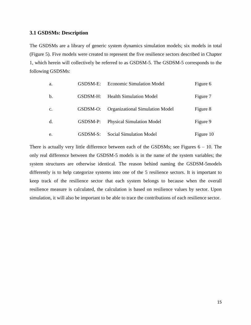
Figure 5: Opening the library of GSDSMs

Figure 6: GSDSM-E; economic generic model structure

17

Figure 7: GSDSM-H; health generic model structure

Figure 8: GSDSM-O; organizational generic model structure

18

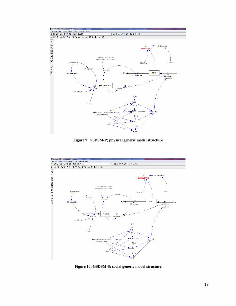
Figure 9: GSDSM-P; physical generic model structure

Figure 10: GSDSM-S; social generic model structure

19

As can be seen in Figures 6 to 10, there are certain variables which are ill defined such as,

climate change, exposure, vulnerability and influence from external factors. These variables are

intended to be “placeholders”. That is, they do not relate directly to the resilience sector system,

but are meant to be linked to other sectors once the GSDSMs are modified and relationships

between the modified GSDSMs have been identified.

The variables robustness, rapidity, resourcefulness and redundancy are measured in the

GSDSMs by indicators. Every performance measure indicator used in the quantification of

impacts and adaptive capacity (the 4 R’s) is compared to a threshold performance indicator value

in order to determine the starting point of system disturbance and the ending point. The

threshold values may be predefined system impact or adaptive capacity standards. This is how

the variables robustness, rapidity, resourcefulness and redundancy are quantified in the

GSDSMs.

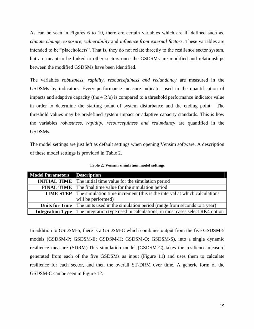
The model settings are just left as default settings when opening Vensim software. A description

of these model settings is provided in Table 2.

Table 2: Vensim simulation model settings

Model Parameters Description

INITIAL TIME The initial time value for the simulation period

FINAL TIME The final time value for the simulation period

TIME STEP The simulation time increment (this is the interval at which calculations

will be performed)

Units for Time The units used in the simulation period (range from seconds to a year)

Integration Type The integration type used in calculations; in most cases select RK4 option

In addition to GSDSM-5, there is a GSDSM-C which combines output from the five GSDSM-5

models (GSDSM-P; GSDSM-E; GSDSM-H; GSDSM-O; GSDSM-S), into a single dynamic

resilience measure (SDRM).This simulation model (GSDSM-C) takes the resilience measure

generated from each of the five GSDSMs as input (Figure 11) and uses them to calculate

resilience for each sector, and then the overall ST-DRM over time. A generic form of the

GSDSM-C can be seen in Figure 12.

20

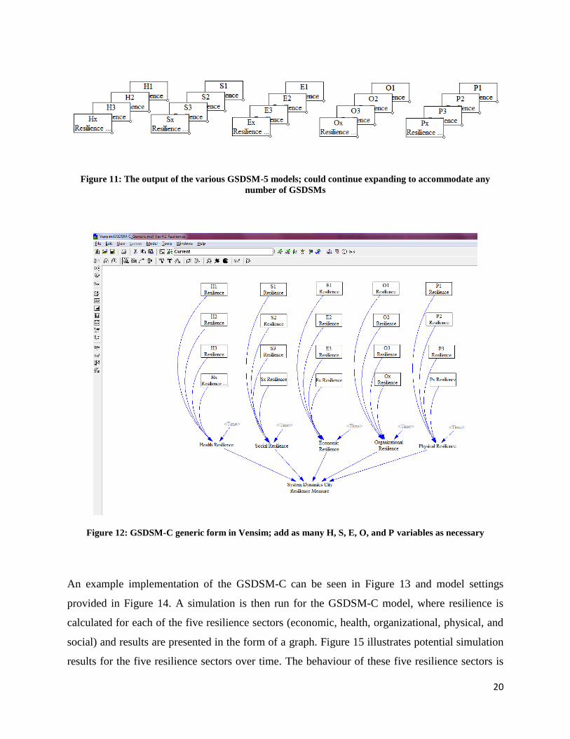
Figure 11: The output of the various GSDSM-5 models; could continue expanding to accommodate any

number of GSDSMs

Figure 12: GSDSM-C generic form in Vensim; add as many H, S, E, O, and P variables as necessary

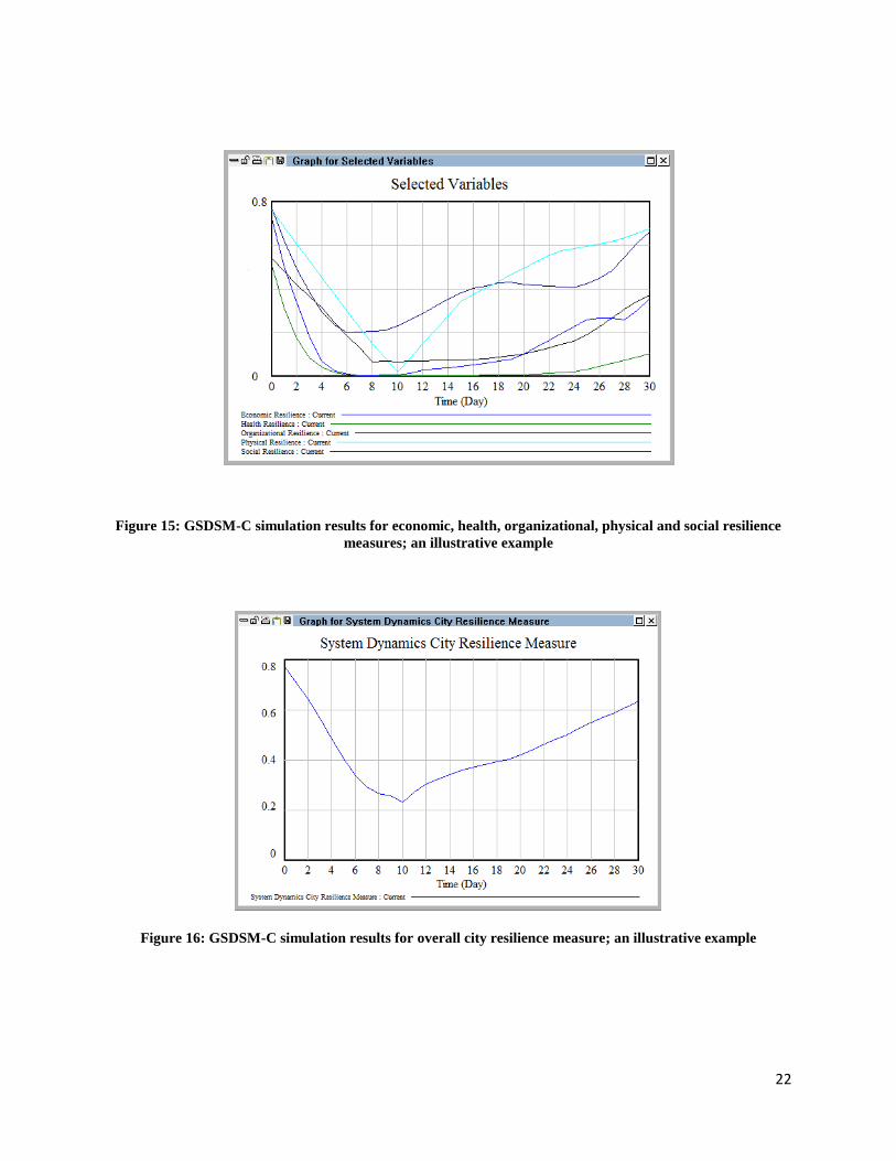
An example implementation of the GSDSM-C can be seen in Figure 13 and model settings

provided in Figure 14. A simulation is then run for the GSDSM-C model, where resilience is

calculated for each of the five resilience sectors (economic, health, organizational, physical, and

social) and results are presented in the form of a graph. Figure 15 illustrates potential simulation

results for the five resilience sectors over time. The behaviour of these five resilience sectors is

21

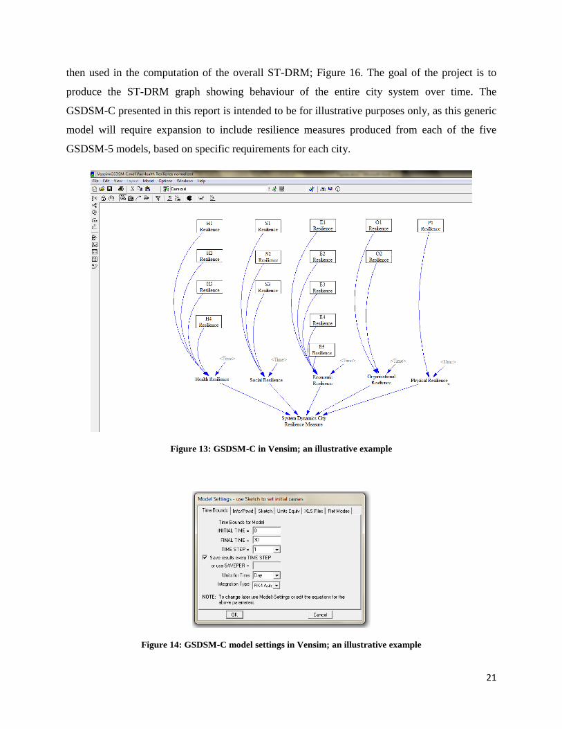
then used in the computation of the overall ST-DRM; Figure 16. The goal of the project is to

produce the ST-DRM graph showing behaviour of the entire city system over time. The

GSDSM-C presented in this report is intended to be for illustrative purposes only, as this generic

model will require expansion to include resilience measures produced from each of the five

GSDSM-5 models, based on specific requirements for each city.

Figure 13: GSDSM-C in Vensim; an illustrative example

Figure 14: GSDSM-C model settings in Vensim; an illustrative example

22

Figure 15: GSDSM-C simulation results for economic, health, organizational, physical and social resilience

measures; an illustrative example

Figure 16: GSDSM-C simulation results for overall city resilience measure; an illustrative example

23

It is expected that there will be many of each of the GSDSM-5 models in order to construct a

meaningful GSDSM-C model and for accurate representation of the ST-DRM. The combination

of both the GSDSM-5 models and GSDSM-C model are referred to as the City Resilience

Simulator (CRS). The goal of the CRS is to capture dynamic relationships and compute ST-

DRM; similar to the GSDSM-C model, but includes the entire system structures of both the

GSDSM-5s and GSDSM-C. The CRS is described in more detail later in this chapter. It should

be noted that the GSDSMs and CRS currently are not spatially distributed. Incorporating the

spatial dimension into GSDSMs will follow in future work.

3.2 GSDSMs: Use

The GSDSMs are generic-structure simulation models created in a Vensim environment to

simplify and improve the process of building a CRS. In order to effectively use the GSDSMs to

do so, it is recommended to follow the generic steps in Table 3. Ideally, begin the GSDSM

process by identifying critical systems; focusing on those services and functional activities that

are essential for a resilient community. The continued operation and rapid restoration of these

critical lifeline services are a necessary condition for overall community resilience. An example

of critical lifeline services is presented in Table 1.

The generic model forms can be modified for the specifics of each coastal city. It is expected that

each coastal megacity will require modifications to be made to the GSDSMs structures to best

reflect local conditions and available data. It is highly recommended that before using the

GSDSMs to develop a CRS, each city develop a high-level causal loop diagram in addition to

identifying: major critical systems, potential impacts, capacities and indicators. Taking these

initial steps will help improve the effectiveness and successful implementation of the GSDSMs.

24

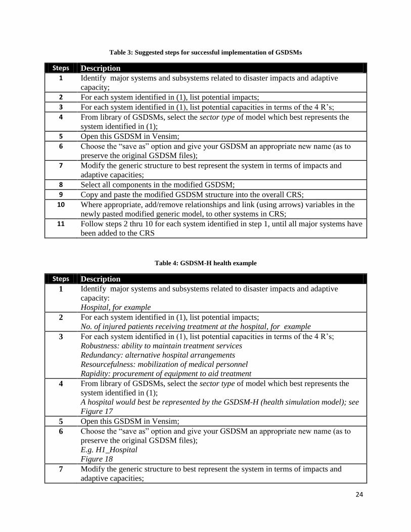
Table 3: Suggested steps for successful implementation of GSDSMs

Steps Description

1 Identify major systems and subsystems related to disaster impacts and adaptive

capacity;

2 For each system identified in (1), list potential impacts;

3 For each system identified in (1), list potential capacities in terms of the 4 R’s;

4 From library of GSDSMs, select the sector type of model which best represents the

system identified in (1);

5 Open this GSDSM in Vensim;

6 Choose the “save as” option and give your GSDSM an appropriate new name (as to

preserve the original GSDSM files);

7 Modify the generic structure to best represent the system in terms of impacts and

adaptive capacities;

8 Select all components in the modified GSDSM;

9 Copy and paste the modified GSDSM structure into the overall CRS;

10 Where appropriate, add/remove relationships and link (using arrows) variables in the

newly pasted modified generic model, to other systems in CRS;

11 Follow steps 2 thru 10 for each system identified in step 1, until all major systems have

been added to the CRS

Table 4: GSDSM-H health example

Steps Description

1 Identify major systems and subsystems related to disaster impacts and adaptive

capacity:

Hospital, for example

2 For each system identified in (1), list potential impacts;

No. of injured patients receiving treatment at the hospital, for example

3 For each system identified in (1), list potential capacities in terms of the 4 R’s;

Robustness: ability to maintain treatment services

Redundancy: alternative hospital arrangements

Resourcefulness: mobilization of medical personnel

Rapidity: procurement of equipment to aid treatment

4 From library of GSDSMs, select the sector type of model which best represents the

system identified in (1);

A hospital would best be represented by the GSDSM-H (health simulation model); see

Figure 17

5 Open this GSDSM in Vensim;

6 Choose the “save as” option and give your GSDSM an appropriate new name (as to

preserve the original GSDSM files);

E.g. H1_Hospital

Figure 18

7 Modify the generic structure to best represent the system in terms of impacts and

adaptive capacities;

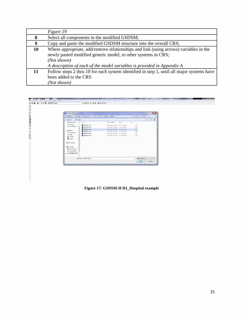
25

Figure 19

8 Select all components in the modified GSDSM;

9 Copy and paste the modified GSDSM structure into the overall CRS;

10 Where appropriate, add/remove relationships and link (using arrows) variables in the

newly pasted modified generic model, to other systems in CRS;

(Not shown)

A description of each of the model variables is provided in Appendix A

11 Follow steps 2 thru 10 for each system identified in step 1, until all major systems have

been added to the CRS

(Not shown)

Figure 17: GSDSM-H H1_Hospital example

26

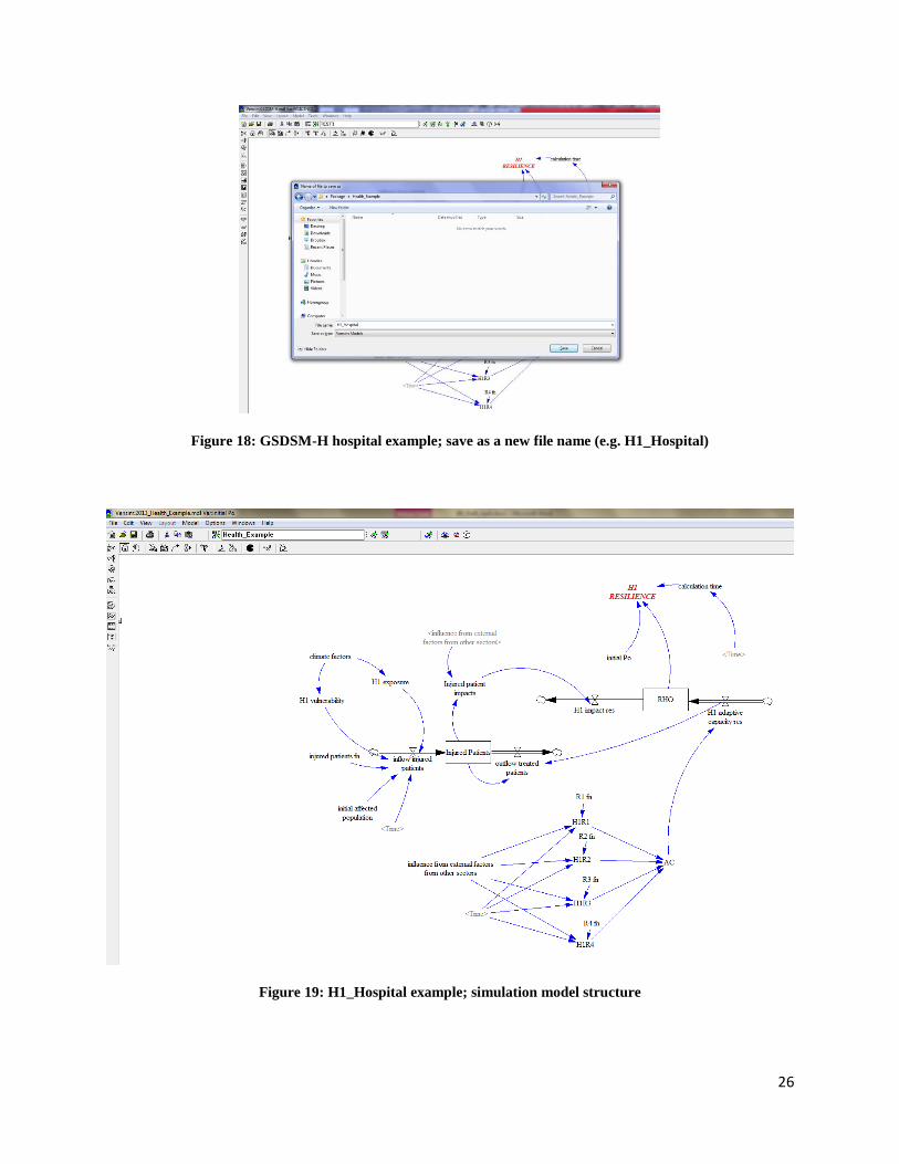
Figure 18: GSDSM-H hospital example; save as a new file name (e.g. H1_Hospital)

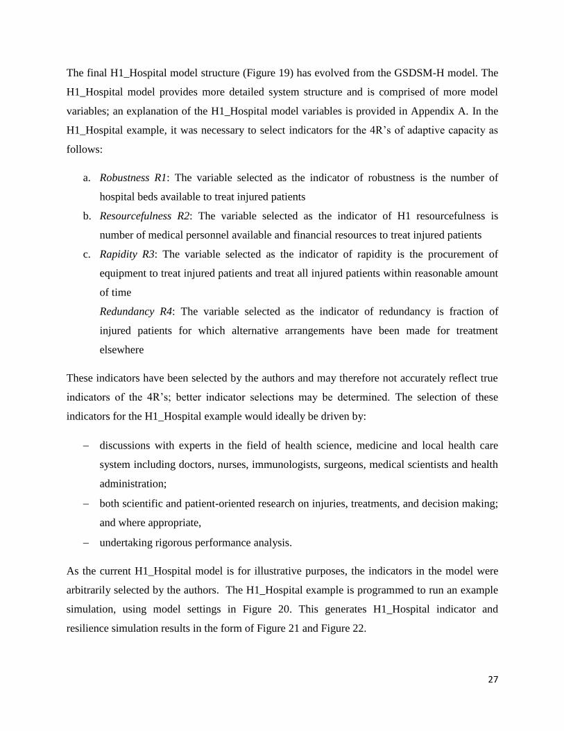
Figure 19: H1_Hospital example; simulation model structure

27

The final H1_Hospital model structure (Figure 19) has evolved from the GSDSM-H model. The

H1_Hospital model provides more detailed system structure and is comprised of more model

variables; an explanation of the H1_Hospital model variables is provided in Appendix A. In the

H1_Hospital example, it was necessary to select indicators for the 4R’s of adaptive capacity as

follows:

a. Robustness R1: The variable selected as the indicator of robustness is the number of

hospital beds available to treat injured patients

b. Resourcefulness R2: The variable selected as the indicator of H1 resourcefulness is

number of medical personnel available and financial resources to treat injured patients

c. Rapidity R3: The variable selected as the indicator of rapidity is the procurement of

equipment to treat injured patients and treat all injured patients within reasonable amount

of time

Redundancy R4: The variable selected as the indicator of redundancy is fraction of

injured patients for which alternative arrangements have been made for treatment

elsewhere

These indicators have been selected by the authors and may therefore not accurately reflect true

indicators of the 4R’s; better indicator selections may be determined. The selection of these

indicators for the H1_Hospital example would ideally be driven by:

discussions with experts in the field of health science, medicine and local health care

system including doctors, nurses, immunologists, surgeons, medical scientists and health

administration;

both scientific and patient-oriented research on injuries, treatments, and decision making;

and where appropriate,

undertaking rigorous performance analysis.

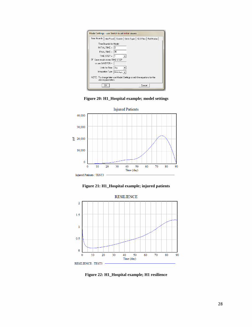
As the current H1_Hospital model is for illustrative purposes, the indicators in the model were

arbitrarily selected by the authors. The H1_Hospital example is programmed to run an example

simulation, using model settings in Figure 20. This generates H1_Hospital indicator and

resilience simulation results in the form of Figure 21 and Figure 22.

28

Figure 20: H1_Hospital example; model settings

Figure 21: H1_Hospital example; injured patients

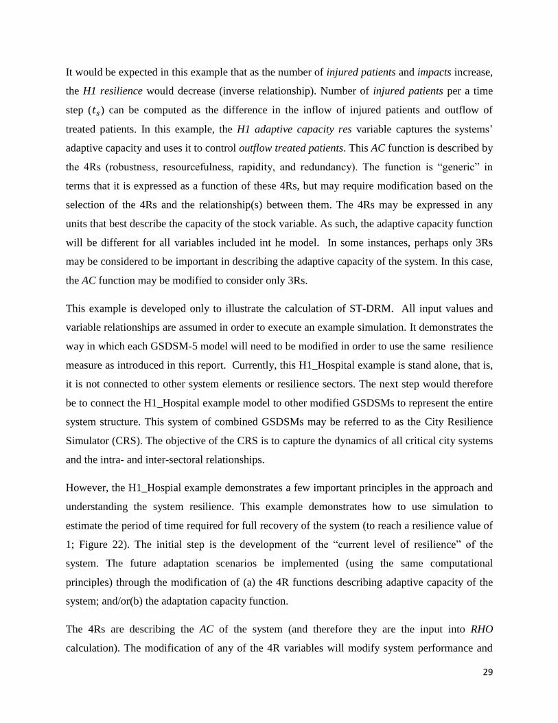
Figure 22: H1_Hospital example; H1 resilience

29

It would be expected in this example that as the number of injured patients and impacts increase,

the H1 resilience would decrease (inverse relationship). Number of injured patients per a time

step ( ) can be computed as the difference in the inflow of injured patients and outflow of

treated patients. In this example, the H1 adaptive capacity res variable captures the systems’

adaptive capacity and uses it to control outflow treated patients. This AC function is described by

the 4Rs (robustness, resourcefulness, rapidity, and redundancy). The function is “generic” in

terms that it is expressed as a function of these 4Rs, but may require modification based on the

selection of the 4Rs and the relationship(s) between them. The 4Rs may be expressed in any

units that best describe the capacity of the stock variable. As such, the adaptive capacity function

will be different for all variables included int he model. In some instances, perhaps only 3Rs

may be considered to be important in describing the adaptive capacity of the system. In this case,

the AC function may be modified to consider only 3Rs.

This example is developed only to illustrate the calculation of ST-DRM. All input values and

variable relationships are assumed in order to execute an example simulation. It demonstrates the

way in which each GSDSM-5 model will need to be modified in order to use the same resilience

measure as introduced in this report. Currently, this H1_Hospital example is stand alone, that is,

it is not connected to other system elements or resilience sectors. The next step would therefore

be to connect the H1_Hospital example model to other modified GSDSMs to represent the entire

system structure. This system of combined GSDSMs may be referred to as the City Resilience

Simulator (CRS). The objective of the CRS is to capture the dynamics of all critical city systems

and the intra- and inter-sectoral relationships.

However, the H1_Hospial example demonstrates a few important principles in the approach and

understanding the system resilience. This example demonstrates how to use simulation to

estimate the period of time required for full recovery of the system (to reach a resilience value of

1; Figure 22). The initial step is the development of the “current level of resilience” of the

system. The future adaptation scenarios be implemented (using the same computational

principles) through the modification of (a) the 4R functions describing adaptive capacity of the

system; and/or(b) the adaptation capacity function.

The 4Rs are describing the AC of the system (and therefore they are the input into RHO

calculation). The modification of any of the 4R variables will modify system performance and

30

ultimately, system resilience behaviour. This is how adaptation scenarios will be effectively

implemented into the model simulation.

4. CITY RESILIENCE SIMULATOR (CRS)

The CRS may be considered the main SD model file which contains modified GSDSMs for all

economic, health, organizational, physical and social resilience systems. The modified GSDSMs

are added to the CRS and the GSDSM model “placeholder” variables (such as “climate change”,

“influence from external factors” and “exposure”) are replaced with connections (links/arrows

in Vensim) to other sectors within the model. The CRS may therefore be considered the

complex, detailed, comprehensive city system simulation model which will simulate the overall

city resilience. Progress of CRS development is directly related to the progress of project

research in different focus areas: physical modelling, social investigations, economic modeling,

health analyses, etc. The results of the work in different impact areas will result in general shape

of the CRS model for each city. At this stage of the project research, the focus has been placed

on the development of the smaller, subsystems of GSDSMs and general model development

procedure. Therefore, there is currently no example of a CRS. The CRS models for each city will

develop from GSDSMs as they become defined, refined and added to the main CRS model.

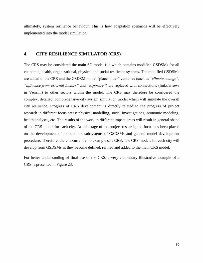
For better understanding of final use of the CRS, a very elementary illustrative example of a

CRS is presented in Figure 23.

31

Figure 23: A conceptual diagram of the CRS structure

When the CRS structure is completely developed (all appropriate economic, health,

organizational, physical and social systems have been modeled using SD software), the CRS

may then be used simulate the change in city resilience as a consequence of various adaptation

options. Set of adaptation options will represent one simulation scenario and comparison of city

resilience (simulation output) will be used in relative evaluation of each option.

In order to capture both the short- and long- term hazard impacts, the CRS will be used in two

different modes:

1. Short term, event, simulation; to capture the more immediate impacts of event-based

short and medium duration climate hazards such as flooding, wind gusts, storms, and

similar; and

2. Long term simulation; to capture the impacts of more gradual, long duration climate

hazards such as sea-level rise.

It is therefore expected that each project city will have both a short- and long- term CRS

simulation model (CRS-N-S and CRS-N-L, respectively; where N represents the first letter in the

name of the project city, for example CRS-V-S would be the CRS short-term simulation model

32

for the project city of Vancouver, Canada). The SD structure between the CRS-N-Sand CRS-N-

L models will be very similar. However, the CRS-N-L may require minor adjustments to system

structure to be able to accommodate long-term simulation period. The CRS-N-S and CRS-N-L

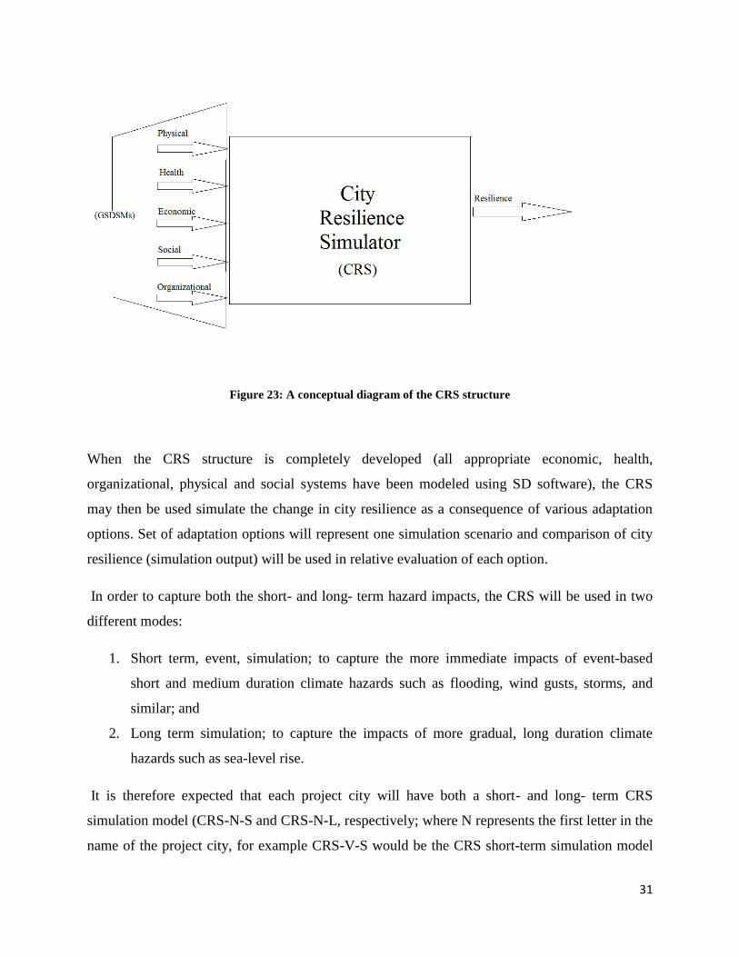
SD model settings will be different. For example, Figure 24 presents possible model settings for

a short term simulation model, where the calculations would be made on a daily time interval

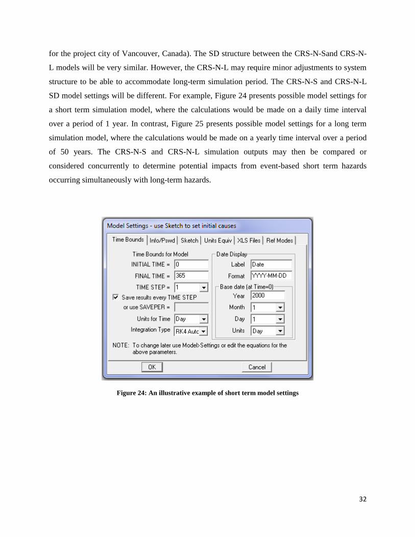
over a period of 1 year. In contrast, Figure 25 presents possible model settings for a long term

simulation model, where the calculations would be made on a yearly time interval over a period

of 50 years. The CRS-N-S and CRS-N-L simulation outputs may then be compared or

considered concurrently to determine potential impacts from event-based short term hazards

occurring simultaneously with long-term hazards.

Figure 24: An illustrative example of short term model settings

33

Figure 25: An illustrative example of long term model settings

5. CONCLUSIONS

This report presents the GSDSMs description, use and implementation for simulation of dynamic

resilience to climate change caused natural disasters in coastal megacities. The purpose of the

GSDSMs is to assist coastal cities in developing their own CRS by using them as a starting point

for CRS model structure. GSDSM users may select from a library of generic simulation models

which can be added to comprehensive CRS. The number of GSDSMs that may be added to each

CRS will depend on each city’s individual local conditions.

For the primary case study city of Vancouver, British Columbia, Canada, the data collection for

the GSDSMs and CRS model inputs is actively being pursued concurrently with the modeling

work through the discussions with local decision makers and other project team members. CRS-

V development is underway and model structure is currently being refined and expanded.

This report outlines the system dynamics framework of CRS and is currently only focused on

temporal dynamics of the resilience measure. However, the future work includes integration of

SD simulation with GIS software so that dynamics of ST-DRM measure will be simulated in

34

both, time and space. The final output will be in the form of dynamic maps which show changes

in resilience over space and in time as a response to an adaptation scenario.

The ultimate goal of the CRS is to simulate and assess various climate change adaptation

scenarios that will provide for policy development. The assessment process will be based on the

analyses of simulated changes in city resilience behaviour over time and space before, during

and after the occurrence of a disaster event. The expectation is that using the CRS to simulate

behaviour in response to various policy options will help: identify disaster-resilient systems,

determine why some systems are more resilient than others, and help prioritize adaptation

actions.

Updates on CRS progress and the CCaR project can be found at the project website:

coastalcitiesatrisk.org/wordpress.

ACKNOWLEDGEMENTS

The authors would like to acknowledge the financial support for the research provided by the

NSERC CGS doctoral scholarship awarded to the first author and by the IDRC to the second

author.

REFERENCES

Akanda, A.S. and Hossain, F. 2012. The Climate-Water-Health Nexus in Emerging Megacities.

EOS Transactions, American Geophysical Union, 93(37), 353-354.

Bruneau, M., Chang, S.E., Eguchi, R.T., Lee, G.C., O’Rourke, T.D., Reinhorn, A.M., Shinozuka,

M., Tierney, K., Wallace, W.A., and von Winterfeldt, D. 2003. A framework to quantitatively

assess and enhance the seismic resilience of communities. Earthquake Spectra, 19(4): 733-

752.

35

Forrester, J. W. 2009. Some Basic Concepts in System Dynamics, Sloan School of Management,

Massachusetts Institute of Technology, 17pgs.

IPCC, 2012. Summary for Policymakers. In: Managing the Risks of Extreme Events and

Disasters to Advance Climate Change Adaptation [Field, C.B., V. Barros, T.F. Stocker, D.

Qin, D.J. Dokken, K.L. Ebi, M.D. Mastrandrea,K.J. Mach, G.-K. Plattner, S.K. Allen, M.

Tignor, and P.M. Midgley (eds.)]. A Special Report of Working GroupsI and II of the

Intergovernmental Panel on Climate Change. Cambridge University Press, Cambridge, UK,

andNew York, NY, USA, pp. 1-19.

Kesavan, P.C. and Swaminathan, M.S. 2006. Managing extreme natural disasters in coastal

areas. Philosophical Transactions: Mathematical, Physical, and Engineering Sciences, vol.

364, no. 1845, 2191-2216.

Owrangi, A., Lannigan, R. and Simonovic, S.P. 2012. Climate Security (Health Section): Outline

of the Proposed Methodology for Developing a Baseline “Health Input” for City Resilience

Model. (Draft for Internal Use), 9pgs.

Paton, D. and Johnston, D. 2006. Disaster Resilience: An Integrated Approach. Charles C.

Thomas Publishers, Ltd., USA.

Simonovic, S.P., and Peck, A. 2013. Dynamic Resilience to Climate Change Caused Natural

Disasters in Coastal Megacities - Quantification Framework. British Journal of Environment

and Climate Change, in print.

United Nations. 2008. An Overview of Urbanization, Internal Migration, Population Distribution

and Development in the World. United Nations Populations Division. New York, USA.

United Nations. 2011. Population Distribution, Urbanization, Internal Migration and

Development: An International Perspective. United Nations Department of Economic and

Social Affairs Population Division. New York, USA.

36

United Nations. 2012. World Urbanization Prospects: The 2011 Revision. Department of

Economic and Social Affairs, Population Division, New York, USA.

Wenzel, F., Bendimerad, F. and Sinha, R. 2007. Megacities – megarisks. Natural Hazards, 42:

481-491.

37

APPENDIX A: Description of variables in the H1_Hospital example

The following is a description of the variables (and units) used in the implementation of the

GSDSM-H example for a hospital (H1_Hospital example).

<Time> (time): This is a shadow variable which provides the current time for each calculation

step during simulation. It appears multiple times in the simulation model, but the value of thgis

variable at all occurrences is the same.

<Influence from external factors from other sectors> (dmnl): This is a shadow variable which is

holding the same name as another variable in the model. Similarly, it is meant to be a

placeholder where possible connections to and influences from other sectors within the overall

CRS model. This could include connections to the economic, transportation, or other health

model sectors. These connections will be different for each system that is being modelled and

has therefore been left in a generic form.

AC (people): A function of the 4Rs. Represents capacity of the system to absorb impacts from

hazard. The 4Rs create this function. This function will be modified for different impacts;

equations will change depending on the relationship between the 4R variables.

Calculation time: This variable is used for the resilience calculation; variable not necessary,

could be programmed right into the H1 Resilience variable calculation, but for simplicity has

been introduced here as a separate variable.

Climate factors (dmnl): This variable represents possible connections to the climate sector;

currently a placeholder variable.

H1 adaptive capacity (dmnl): This variable is calculated using the 4R properties of adaptive

capacity for an H1_Hospital system, including rapidity, redundancy, resourcefulness and

robustness. It is a combination of the normalized 4R properties and will therefore have a solution

between [0, 4], as calculated in equation (1).

38

H1 exposure (dmnl): Represents the degree of exposure to a climate hazard. This variables’

value is dependent on the type of hazard; in a flooding situation, this variable may be considered

the aerial extent of flooding and depth of water; currently a placeholder variable for future

connections to the climate sector.

H1 Resilience (dmnl): The resilience calculation for the H1 system. This variable is calculated

using equation (4) as the area under the system performance curve based on the initial

performance level, Po. H1 adaptive capacity res (people per time): this variable is actually the

inflow rate (per time step) which modifies the RHO variable. It is the adaptive capacity value,

expressed as a rate, in the same units as the indicator (i.e. Injured Patients).

H1 resilience impacts res (people per time): This variable is actually the outflow rate (per time

step) which modifies the H1 Resilience variable. It is the impacts value, expressed as a rate. It is

the impacts value, expressed as a rate, in the same units as the indicator (i.e. Injured Patients).

H1R1 (people): (i.e. robustness) This variable calls the R1 fn which, for the purposes of this

example, is used as an indicator for H1 system robustness. This variable looks up the value of R1

at time t, in the model.

H1R2 (people): (i.e. resourcefulness) This variable calls the R2 fn which for the purposes of this

example, is used as an indicator for H1 system resourcefulness. This variable looks up the value

of R2 at time t, in the model.

H1R3 (dmnl): (i.e. rapidity) This variable calls the R3 fn which for the illustrative purposes of

this example, is used as an indicator for H1 system rapidity. This variable looks up the value of

R4 at time t, in the model.

H1R4 (dmnl): (i.e. redundancy) This variable calls the R4 fn which for the illustrative purposes

of this example, is used as an indicator for H1 system redundancy. This variable looks up the

value of R4 at time t.

H1 vulnerability (dmnl): Represents characteristics that may make a person, place, or thing more

susceptible to suffering negative consequences; in the health example case, this could be

39

considered those people who are very young or very old and more prone to injury in the event of

a disaster.

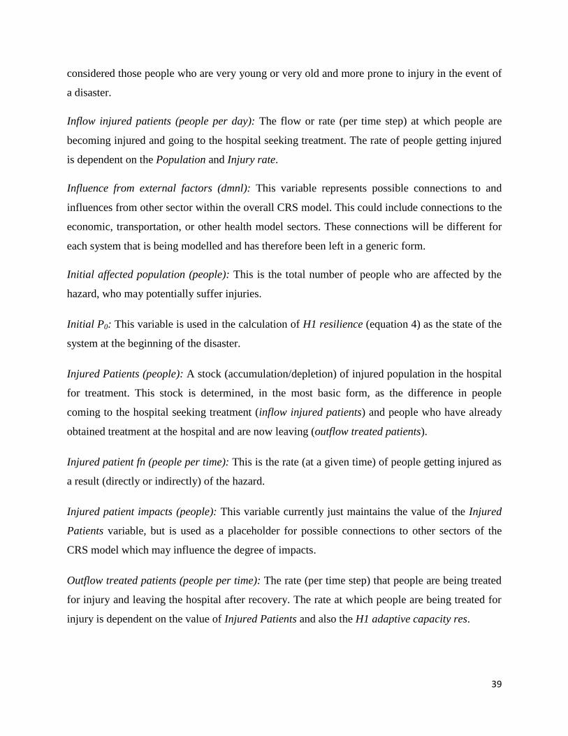
Inflow injured patients (people per day): The flow or rate (per time step) at which people are

becoming injured and going to the hospital seeking treatment. The rate of people getting injured

is dependent on the Population and Injury rate.

Influence from external factors (dmnl): This variable represents possible connections to and

influences from other sector within the overall CRS model. This could include connections to the

economic, transportation, or other health model sectors. These connections will be different for

each system that is being modelled and has therefore been left in a generic form.

Initial affected population (people): This is the total number of people who are affected by the

hazard, who may potentially suffer injuries.

Initial P0: This variable is used in the calculation of H1 resilience (equation 4) as the state of the

system at the beginning of the disaster.

Injured Patients (people): A stock (accumulation/depletion) of injured population in the hospital

for treatment. This stock is determined, in the most basic form, as the difference in people

coming to the hospital seeking treatment (inflow injured patients) and people who have already

obtained treatment at the hospital and are now leaving (outflow treated patients).

Injured patient fn (people per time): This is the rate (at a given time) of people getting injured as

a result (directly or indirectly) of the hazard.

Injured patient impacts (people): This variable currently just maintains the value of the Injured

Patients variable, but is used as a placeholder for possible connections to other sectors of the

CRS model which may influence the degree of impacts.

Outflow treated patients (people per time): The rate (per time step) that people are being treated

for injury and leaving the hospital after recovery. The rate at which people are being treated for

injury is dependent on the value of Injured Patients and also the H1 adaptive capacity res.

40

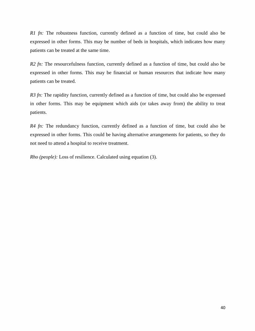
R1 fn: The robustness function, currently defined as a function of time, but could also be

expressed in other forms. This may be number of beds in hospitals, which indicates how many

patients can be treated at the same time.

R2 fn: The resourcefulness function, currently defined as a function of time, but could also be

expressed in other forms. This may be financial or human resources that indicate how many

patients can be treated.

R3 fn: The rapidity function, currently defined as a function of time, but could also be expressed

in other forms. This may be equipment which aids (or takes away from) the ability to treat

patients.

R4 fn: The redundancy function, currently defined as a function of time, but could also be

expressed in other forms. This could be having alternative arrangements for patients, so they do

not need to attend a hospital to receive treatment.

Rho (people): Loss of resilience. Calculated using equation (3).

41

APPENDIX B: Description of the Distribution Package

The package of models distributed with this report to the project team includes the following:

a. GSDSMs-5

This sub-folder includes the following five generic system dynamics simulation models:

a. GSDSM-E

The generic economics sector system dynamics simulation model

b. GSDSM-H

The generic health sector system dynamics simulation model

c. GSDSM-O

The generic organizational sector system dynamics simulation model

d. GSDSM-P

The generic physical sector system dynamics simulation model

e. GSDSM-S

The generic social sector system dynamics simulation model

*None of these models include equations or even all the links that may be necessary to

accurately represent the system. Instead, these generic models are meant to act as a

graphical foundation for building sectors that will be modified before being included in a

CRS.

b. GSDSM-C

The Vensim model which would combine all of the city system resiliencies into a single

overall resilience measure (ST-DRM) as indicated in Equation (7). The number of

systems in each sector (economic, health, organizational, physical and social) will vary

for each project city and then be used in ST-DRM calculation. The functions currently

used to represent each system (H1, H2, H3,…, Hn) are assumed for illustrative purposes

and are not based on real values.

42

c. Health Example H1

An example in Vensim SD software to illustrate the use of GSDSM-H for a hospital

system, defined in this case as a health system H1. Appendix A provides a description of

the model and its variables. Please note that the actual values provided in this model are

selected by the authors for the purposes of illustrating GSDSM-H model development

and simulation. The current assumption in this example is that the disaster event (system

disturbance) starts at time 0.

43

APPENDIX C: List of Previous Reports in the Series ISSN: (print) 1913-3200; (online) 1913-3219

In addition to 53 previous reports (no. 01 – no. 53) prior to 2007;

(1) Predrag Prodanovic and Slobodan P. Simonovic (2007). Dynamic Feedback Coupling of Continuous Hydrologic

and Socio-Economic Model Components of the Upper Thames River Basin. Water Resources Research Report no.

054, Facility for Intelligent Decision Support, Department of Civil and Environmental Engineering, London,

Ontario, Canada, 437 pages. ISBN: (print) 978-0-7714-2638-4; (online) 978-0-7714-2639-1.

(2) Subhankar Karmakar and Slobodan P. Simonovic (2007). Flood Frequency Analysis Using Copula with Mixed

Marginal Distributions. Water Resources Research Report no. 055, Facility for Intelligent Decision Support,

Department of Civil and Environmental Engineering, London, Ontario, Canada, 144 pages. ISBN: (print) 978-0-

7714-2658-2; (online) 978-0-7714-2659-9.

(3) Jordan Black, Subhankar Karmakar and Slobodan P. Simonovic (2007). A Web-Based Flood Information

System. Water Resources Research Report no. 056, Facility for Intelligent Decision Support, Department of Civil

and Environmental Engineering, London, Ontario, Canada, 133 pages. ISBN: (print) 978-0-7714-2660-5; (online)

978-0-7714-2661-2.

(4) Angela Peck, Subhankar Karmakar and Slobodan P. Simonovic (2007). Physical, Economical, Infrastructural

and Social Flood Risk – Vulnerability Analyses in GIS. Water Resources Research Report no. 057, Facility for

Intelligent Decision Support, Department of Civil and Environmental Engineering, London, Ontario, Canada, 80

pages. ISBN: (print) 978-0- 7714-2662-9; (online) 978-0-7714-2663-6.

(5) Predrag Prodanovic and Slobodan P. Simonovic (2007). Development of Rainfall Intensity Duration Frequency

Curves for the City of London Under the Changing Climate. Water Resources Research Report no. 058, Facility for


pages. ISBN: (print) 978-0- 7714-2667-4; (online) 978-0-7714-2668-1.

(6) Evan G. R. Davies and Slobodan P. Simonovic (2008). An integrated system dynamics model for analyzing

behaviour of the social-economic-climatic system: Model description and model use guide. Water Resources

Research Report no. 059, Facility for Intelligent Decision Support, Department of Civil and Environmental

Engineering, London, Ontario, Canada, 233 pages. ISBN: (print) 978-0-7714-2679-7; (online) 978-0-7714-2680-3.

(7) Vasan Arunachalam (2008). Optimization Using Differential Evolution. Water Resources Research Report no.


Ontario, Canada, 42 pages. ISBN: (print) 978-0-7714- 2689-6; (online) 978-0-7714-2690-2.

(8) Rajesh Shrestha and Slobodan P. Simonovic (2009). A Fuzzy Set Theory Based Methodology for Analysis of

Uncertainties in Stage-Discharge Measurements and Rating Curve. Water Resources Research Report no. 061,

44

Facility for Intelligent Decision Support, Department of Civil and Environmental Engineering, London, Ontario,

Canada, 104 pages. ISBN: (print) 978-0-7714-2707-7; (online) 978-0-7714-2708-4.

(9) Hyung-Il Eum, Vasan Arunachalam and Slobodan P. Simonovic (2009). Integrated Reservoir Management

System for Adaptation to Climate Change Impacts in the Upper Thames River Basin. Water Resources Research

Report no. 062, Facility for Intelligent Decision Support, Department of Civil and Environmental Engineering,

London, Ontario, Canada, 81 pages. ISBN: (print) 978-0-7714-2710-7; (online) 978-0-7714-2711-4.

(10) Evan G. R. Davies and Slobodan P. Simonovic (2009). Energy Sector for the Integrated System Dynamics

Model for Analyzing Behaviour of the Social- Economic-Climatic Model. Water Resources Research Report no.

063. Facility for Intelligent Decision Support, Department of Civil and Environmental Engineering, London,

Ontario, Canada. 191 pages. ISBN: (print) 978-0-7714-2712-1; (online) 978-0-7714-2713-8.

(11) Leanna King, Tarana Solaiman, and Slobodan P. Simonovic (2009). Assessment of Climatic Vulnerability in

the Upper Thames River Basin. Water Resources Research Report no. 064, Facility for Intelligent Decision Support,

Department of Civil and Environmental Engineering, London, Ontario, Canada, 61pages. ISBN: (print) 978-0-7714-

2816-6; (online) 978-0-7714- 2817-3.

(12) Slobodan P. Simonovic and Angela Peck (2009). Updated Rainfall Intensity Duration Frequency Curves for the

City of London under Changing Climate. Water Resources Research Report no. 065, Facility for Intelligent

Decision Support, Department of Civil and Environmental Engineering, London, Ontario, Canada, 64pages. ISBN:

(print) 978-0-7714-2819-7; (online) 987-0-7714-2820-3.

(13) Leanna King, Tarana Solaiman, and Slobodan P. Simonovic (2010). Assessment of Climatic Vulnerability in

the Upper Thames River Basin: Part 2. Water Resources Research Report no. 066, Facility for Intelligent Decision

Support, Department of Civil and Environmental Engineering, London, Ontario, Canada, 72pages. ISBN: (print)

978-0-7714-2834-0; (online) 978-0-7714-2835-7.

(14) Christopher J. Popovich, Slobodan P. Simonovic and Gordon A. McBean (2010). Use of an Integrated System

Dynamics Model for Analyzing Behaviour of the Social-Economic-Climatic System in Policy Development. Water

Resources Research Report no. 067, Facility for Intelligent Decision Support, Department of Civil and

Environmental Engineering, London, Ontario, Canada, 37 pages. ISBN: (print) 978-0-7714-2838-8; (online) 978-0-

7714-2839-5.

(15) Hyung-Il Eum and Slobodan P. Simonovic (2009). City of London: Vulnerability of Infrastructure to Climate

Change; Background Report 1 – Climate and Hydrologic Modeling. Water Resources Research Report no. 068,


Canada, 102pages. ISBN: (print) 978-0-7714-2844-9; (online) 978-0-7714-2845-6.

(16) Dragan Sredojevic and Slobodan P. Simonovic (2009). City of London: Vulnerability of Infrastructure to

Climate Change; Background Report 2 – Hydraulic Modeling and Floodplain Mapping. Water Resources Research

45



(17) Tarana A. Solaiman and Slobodan P. Simonovic (2011). Quantifying Uncertainties in the Modelled Estimates

of Extreme Precipitation Events at the Upper Thames River Basin. Water Resources Research Report no. 070,



(18) Tarana A. Solaiman and Slobodan P. Simonovic (2011). Assessment of Global and Regional Reanalyses Data

for Hydro-Climatic Impact Studies in the Upper Thames River Basin. Water Resources Research Report no. 071,



(19) Tarana A. Solaiman and Slobodan P. Simonovic (2011). Development of Probability Based Intensity-Duration-

Frequency Curves under Climate Change. Water Resources Research Report no. 072, Facility for Intelligent

Decision Support, Department of Civil and Environmental Engineering, London, Ontario, Canada, 89 pages. ISBN:

(print) 978-0-7714-2893-7; (online) 978-0-7714-2900-2.

(20) Dejan Vucetic and Slobodan P. Simonovic (2011). Water Resources Decision Making Under Uncertainty.

Water Resources Research Report no. 073, Facility for Intelligent Decision Support, Department of Civil and

Environmental Engineering, London, Ontario, Canada, 143 pages. ISBN: (print) 978-0-7714-2894-4; (online) 978-

0-7714-2901-9.

(21) Angela Peck, Elisabeth Bowering and Slobodan P. Simonovic (2010). City of London: Vulnerability of

Infrastructure to Climate Change, Final Report - Risk Assessment. Water Resources Research Report no. 074,



(22) Akhtar, M. K., S. P. Simonovic, J. Wibe, J. MacGee, and J. Davies, (2011). An integrated system dynamics

model for analyzing behaviour of the social-energy-economic-climatic system: model description. Water Resources



(23) Akhtar, M. K., S. P. Simonovic, J. Wibe, J. MacGee, and J. Davies, (2011). An integrated system dynamics

model for analyzing behaviour of the social-energy-economic-climatic system: user’s manual. Water Resources



(24) Millington, N., S. Das and S. P. Simonovic (2011). The Comparison of GEV, Log-Pearson Type 3 and Gumbel

Distributions in the Upper Thames River Watershed under Global Climate Models. Water Resources Research



46

(25) Andre Schardong and Slobodan P. Simonovic (2012). Multi-objective Evolutionary Algorithms for Water

Resources Management. Water Resources Research Report no. 078, Facility for Intelligent Decision Support,

Department of Civil and Environmental Engineering, London, Ontario, Canada, 167 pages. ISBN: (print) 978-0-

7714-2907-1; (online) 978-0-7714-2908-8.

(26) Samiran Das and Slobodan P. Simonovic (2012). Assessment of Uncertainty in Flood Flows under Climate

Change: the Upper Thames River basin (Ontario, Canada). Water Resources Research Report no. 079, Facility for


pages. ISBN: (print) 978-0-7714-2960-6; (online) 978-0-7714-2961-3.

(27) Rubaiya Sarwar, Sarah E. Irwin, Leanna M. King and Slobodan P. Simonovic (2012). Assessment of Climatic

Vulnerability in the Upper Thames River basin: Downscaling with SDSM. Water Resources Research Report no.



(28) Sarah E. Irwin, Rubaiya Sarwar, Leanna King and Slobodan P. Simonovic (2012).Assessment of Climatic

Vulnerability in the Upper Thames River basin: Downscaling with LARS-WG. Water Resources Research Report

no. 081, Facility for Intelligent Decision Support, Department of Civil and Environmental Engineering, London,


(29) Samiran Das and Slobodan P. Simonovic. (2012). Guidelines for Flood Frequency Estimation under Climate

Change. Water Resources Research Report no. 082, Facility for Intelligent Decision Support, Department of Civil

and Environmental Engineering, London, Ontario, Canada, 44 pages. ISBN: (print) 978-0-7714-2973-6; (online)

978-0-7714-2974-3.

http://www.eng.uwo.ca/research/iclr/fids/publications/products/81.pdf

http://www.eng.uwo.ca/research/iclr/fids/publications/products/81.pdf

Documents

Water Resources Research Report - Western Engineering · 2017-07-24 · Coastal cities are particularly threatened by hydro-meteorological climate hazards including: hurricanes, tsunamis,