THE UNIVERSITY OF WESTERN ONTARIO

DEPARTMENT OF CIVIL AND

ENVIRONMENTAL ENGINEERING

Water Resources Research Report

Report No: 058

Date: November 2007

Development of rainfall intensity duration

frequency curves for the City of London

under the changing climate

By:

Predrag Prodanovic

and

Slobodan P. Simonovic

ISSN: (print) 1913-3200; (online) 1913-3219;

ISBN: (print) 978-0-7714-2667-4; (online) 978-0-7714-2668-1;

Development of rainfall intensity duration frequency curves for the City of London under the changing

climate

By:

Predrag Prodanovic and

Slobodan P. Simonovic

Department of Civil and Environmental Engineering The University of Western Ontario

London, Ontario, Canada

November 2007

Executive summary The main focus of this study is the analysis of short duration high intensity rainfall for London, Ontario under the conditions of the changed climate. Predicted future climate change impacts for Southwestern Ontario include higher temperatures and increases in precipitation, leading to an intensification of the hydrologic cycle. One of the expected consequences of change is an increase in the magnitude and frequency of extreme events (e.g. high intensity rainfall, flash flooding, severe droughts, etc.). Changes in extreme events are of particular importance to the design, operation and maintenance of municipal water management infrastructure. Municipal water management infrastructure (sewers, storm water management ponds or detention basins, street curbs and gutters, catchbasins, swales, etc) designs are typically based on the use of local rainfall Intensity Duration Frequency (IDF) curves. IDF curves are developed using historical rainfall time series data. Annual extreme rainfall is fitted to a theoretical probability distribution from which rainfall intensities, corresponding to particular durations, are obtained. In the use of this procedure an assumption is made that historic extremes can be used to characterize extremes of the future (i.e., the historic record is assumed to be stationary). This assumption is not valid under changing climatic conditions that may bring shifts in the magnitude and frequency of extreme rainfall. Such shifts in extreme rainfall at the local level demand new regulations for water infrastructure management as well as changes in design practices. The objective of this report is to assess the change in IDF curves for use by the City of London under changing climatic conditions. The methodology implemented to assess changes in rainfall magnitude resulting from climate change includes the following components: (a) Development and use of a daily weather generator model for synthetic generation of rainfall under current and future climates; (b) Disaggregation of daily rainfall into hourly; (c) Statistical analysis of rainfall of various durations, and development of IDF curves under changed climatic conditions; (d) Comparative analysis of IDF curves; and (e) Recommendation for possible modification of municipal infrastructure design standards. The two IDF curves currently used by the City of London (i.e., MacLauren IDF curve for design of conveyance systems, and Atmospheric Environment Service IDF curve for storm water management facilities) could have not be reproduced in this research using the data currently available from Meteorological Service of Canada. The IDF curves in use by the City are based on data sets that are no longer available. In addition, methods used by either MacLauren or Meteorological Service of Canada to estimate rainfall quantiles for durations shorter than one hour are not available. Therefore, comparing the IDF curves generated in this research to those currently used by the City of London is not appropriate. More confidence is placed in the relative difference between the three scenarios generated in this research: simulated historic climate (no change), and wet and dry climates (change guided by outputs of global circulation model outputs).

2

The results of simulations in this research indicate that rainfall magnitude (as well as intensity) will be different than historically observed. The climate change scenario recommended for use in the evaluation of storm water management design standards (i.e., the wet scenario) reveals a significant increase in rainfall magnitude (and intensity) for a range of durations and return periods. This increase has major implications on the ways in which current (and future) municipal water management infrastructure is designed, operated, and maintained. The main recommendation from this work is that the design standards and guidelines currently employed by the City of London be reviewed and/or revised in light of the information presented in this report. Keywords: K-NN weather generator modelling, intensity-duration-frequency curves, climate change impact modelling, extreme rainfall events.

3

Contents List of Tables, 5 List of Figures, 5 1. Introduction and background, 6

1.1. The problem of climate change at the municipal level, 6 1.2. Global circulation models, 7 1.3. Weather generating models, 8 1.4. Outline of the report, 8

2. Methodology, 10

2.1. Rainfall interpolation, 10 2.2. Formulation of changed climate scenarios, 11 2.3. Daily K-Nearest Neighbour weather generating model, 11 2.4. Nearest neighbour disaggregation of daily rainfall, 15 2.5. Model performance testing, 17 2.6. Rainfall intensity duration frequency analysis, 18

3. Results and analysis, 20

3.1. Rainfall data, 20 3.2. Climate scenarios, 22 3.3. Application of methodology to the City of London, 23 3.4. Verification of weather generator output, 24 3.5. Short duration rainfall under the changing climate, 26 3.6. Sensitivity analysis, 31

4. Conclusions and recommendations, 32

4.1. Current water management design standards, 32 4.2. Recommended modifications, 35

Bibliography, 36 Appendix,

A IPCC Scenarios, 39 B MSC IDF information for London from 2001, 40 C Communication with MSC, 44 D Intensity duration frequency plots, 46

4

List of Tables 1: Meteorological Service of Canada rain gauges, 20 2: Monthly precipitation change fields, 23 1: Summary of weather generator simulation scenarios, 26 4: Extreme rainfall for London: undisturbed historic and MSC 2001, 27 5: IDF for London: historic, dry and wet WG output scenarios, 28 6: IDF for London: use of stations within a 100 km radius of London, 33 7: Percent difference between 100 and 200 km simulations, 34

List of Figures 1: Meteorological stations used in the study, 21 2: Weather generator statistics for the London station, 25 3: Intensity duration frequency plots for London, 29 4: IDF curves for London: undisturbed historic, historic and MSC, 30 5: IDF curves for London: historic, dry and wet WG output, 31 6: London IDF curve for historic WG scenario, 46 7: London IDF curve for dry WG scenario, 47 8: London IDF curve for wet WG scenario, 48 9: London IDF curve for undisturbed historic scenario, 49 10: London IDF curved computed by MSC in 2001, 50

5

1.0 Introduction and background

1.1 The problem of climate change at the municipal level Increased industrial activity during the last century and a half has increased concentration of carbon dioxide in Earth's atmosphere. This has in turn initiated large scale atmospheric processes resulting in change of global temperature and precipitation (among other variables). Changes in Earth's climate system can disrupt the delicate balance of the hydrologic cycle and can eventually lead to increased occurrence of extreme events (such as floods, droughts, heat waves, summer and ice storms, etc.). For municipalities, changed frequency of extreme events (such as intense rainfall, heavy winds and/or ice storms) are of particular importance as adequate procedures, plans and management strategies must be put in place to deal with them (Mehdi et al., 2006). One way of reducing vulnerability to adverse impacts of climate change is to anticipate their possible effects, and adapt; the other is to actually reduce the rate of carbon dioxide released into the atmosphere. Reducing climate change vulnerability means that municipal decision makers and stakeholders need to understand its effects, and develop suitable measures to deal with them in the future. The report by Mehdi et al. (2006) outlines a number of important points regarding why municipal decision makers need to consider climate change. The main point is that “even small shifts in climate normals will have potentially large ramifications for existing infrastructure.” Further, the report states that climate change “will affect municipalities large and small, urban and rural, and have positive and negative consequences for the various type of municipal infrastructure, e.g., roads and bridges; natural systems, e.g., watersheds and forests; and human system, e.g., health and education” (Mehdi et al., 2006, p. 7). Of all possible impacts resulting from changed climatic conditions at the municipal level, this research focuses on those resulting from changes in extreme rainfall. Any change in extreme rainfall could demand new regulations in the form of storm water management strategies, guidelines and design practices, as well as altered municipal infrastructure design standards. In some cases changing hydro-climatic conditions may also require upgrading, retrofitting, rebuilding, or even constructing additional water management infrastructure. The current design standards are based on historic climate information and required level of protection from natural phenomena. For example, a dyke designed to resist a 100 yr flood event (meaning that each year the probability of occurrence of a flood exceeding the design value is 0.01) will, if rainfall magnitude increases, provide significantly lower level of protection (Prodanovic and Simonovic, 2006). With changing climate, it is necessary to thoroughly review and/or update the current design standards for municipal water management infrastructure in order to prevent the possibility of future infrastructure performing below its designed guideline. The objective of this research is to provide data and information necessary for design guidelines modification in order to take into consideration the impact of changing

6

climatic conditions. Since design standards for much of municipal water management infrastructure depend on rainfall, information is therefore provided regarding how rainfall (and extreme rainfall events in particular) is expected to change as climate changes. Synthesis of this research is presented in the form of intensity-duration-frequency (IDF) curves, for a number of different future climate scenarios.

1.2 Global circulation models Currently, one of the best ways to study the effects of climate change is to use global circulation models. These models are the current state of the art in climate science. Their aim is to describe the functioning of the climate system through the use of physics, fluid mechanics, chemistry, as well as other sciences. More specifically, all global circulation models discretise the planet and its atmosphere into a large number of three dimensional cells - these can be thought of as a large number of checker boards stacked on top of each other (Kolbert, 2006, p. 100) - to which relevant equations are applied. In general, there are two different types of equations that are used in all global circulation models - those describing fundamental governing physical laws, and those that are termed empirical (based on observed phenomena that are only partially understood). The former are representations of fundamental equations of motion, laws of thermodynamics, conservation of mass and energy, etc, and are well known; the latter, however, are those phenomena that are observed, but for which sound theory does not yet exist (i.e., small scale processes such as land use that can influence large scale processes such as the global circulation). For most studies that are concerned with the response of a smaller area (such as a city) to a changed climatic signal, the global models are inappropriate because they have spacial and temporal scales that are incompatible with those of a city. One way around this is to still use the global input, but scale it appropriately for the area under consideration. Traditional way of studying the impacts of climatic change for small areas involves scaling down the outputs from global circulation models (temporally and spatially) from which user and location specific impacts are derived. A number of studies have implemented such methodologies, and thus estimated local impacts of climatic change (Coulibaly and Dibike, 2004; Palmer et al., 2004; Southam et al., 1999). However, a number of uncertainties are inherent to this approach. First, the global models have temporal scales that are sometimes incompatible with temporal scales of interest at the local level. The global models are only able to produce monthly outputs with a higher degree of accuracy. This is insufficient since at the local level we are often interested in changes in frequency of occurrence of short-duration high-intensity events, especially when studying the problem of flooding. Temporal downscaling of monthly global output must therefore be employed, and shorter duration events be estimated, thus compounding uncertainty. Second, spacial scales of global models are also incompatible with spacial scales at the local level. The global models typically have grid cells of 100 km by 100 km, and are thus significantly larger than most watersheds (for example, City of London, Ontario covers an area of about 420 km2). Coarse resolution of global models is thus

7

inadequate for the representation of many physical processes of interest at the local scales (including extreme rainfall).

1.3 Weather generating models One way of addressing the temporal and spacial uncertainties is to use weather generating models. Weather generating models are stochastic simulation tools that synthetically create climate information for an area by using both, local and global weather data. The local data includes historically observed data taken from area weather stations in and around the study area, while the global data includes outputs obtained from global circulation models. The former acts to address the fine spacial and temporal scale needed for impact studies, while the later provides the direction of change of the climate (wetter, drier, cooler, etc). Weather generators are usually classified in two categories (for further details see the paper by Sharif and Burn, 2006a): parametric and non-parametric. The parametric weather generators are stochastic tools that generate weather data by assuming a probability distribution function and a large number of parameters (often site specific) for the variables of interest. The non-parametric tools do not make distribution assumptions or have site specific parameters, but rely on various shuffling and sampling algorithms. A common limitation of the parametric weather generators is that they have difficulties representing persistent events such as droughts or prolonged rainfall (Sharif and Burn, 2006a, p. 181). The non-parametric weather generators alleviate these drawbacks, and one of them is thus adopted in this research. The weather generator takes as input historical climate information for a number of weather stations in the area, as well as inputs from global circulation models, and generates climatic information for an arbitrary long period of time for the local weather stations. Sophisticated algorithms are used to shuffle (and perturb) the historical data, and thus generate statistically similar climate - here referred to as the historically identical, or base case scenario. The weather generator is not used solely for the replication of historical trends; it also contains various perturbation mechanisms to generate climatic information not observed in the historic record. The perturbation mechanisms are necessary as long records of historic data are often not available (particularly for shorter durations), or if available, contain a large percentage of missing values. Use of perturbation mechanisms assumes that historic data (of short records) does not capture extreme characteristics likely to be observed in longer data sets. Therefore, they are used to push the observed data outside the historic range, thus providing extremes not been previously recorded. Estimation of extreme rainfall from short data records can underestimate critical values used in the design of municipal infrastructure. Using weather generators with perturbation mechanisms and inputs from global circulation models can therefore produce adequate synthetic data of high spacio-temporal resolution.

1.4 Outline of the report The rest of this report is organized as follows: Section 2 presents the methodology used in the study. It provides technical details regarding (i) rainfall interpolation; (ii)

8

formulation of climate change scenarios; (iii) daily K-Nearest Neighbour weather generating algorithm; (iv) disaggregation of daily into hourly values (also based on the K-Nearest Neighbour algorithm); (v) statistics used to test the model performance; and (vi) the method used to construct the intensity duration frequency curve. Section 3 shows details regarding the application of the methodology to the City of London, and includes historic rainfall data analysis, climate change scenarios and the application of the weather generator model. It also presents the weather generator model verification, as well as intensity duration frequency curves under different climatic conditions. The report in Section 4 ends with concluding remarks, where current water management design standards are reviewed, and possible changes for the future recommended.

9

2.0 Methodology

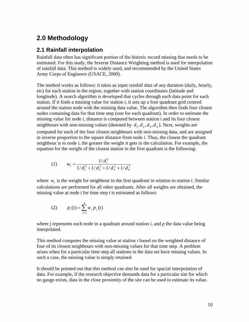
2.1 Rainfall interpolation Rainfall data often has significant portion of the historic record missing that needs to be estimated. For this study, the Inverse Distance Weighting method is used for interpolation of rainfall data. This method is widely used, and recommended by the United States Army Corps of Engineers (USACE, 2000). The method works as follows: it takes as input rainfall data of any duration (daily, hourly, etc) for each station in the region, together with station coordinates (latitude and longitude). A search algorithm is developed that cycles through each data point for each station. If it finds a missing value for station i, it sets up a four quadrant grid centred around the station node with the missing data value. The algorithm then finds four closest nodes containing data for that time step (one for each quadrant). In order to estimate the missing value for node i, distance is computed between station i and its four closest neighbours with non-missing values (denoted by ). Next, weights are

computed for each of the four closest neighbours with non-missing data, and are assigned in inverse proportion to the square distance from node i. Thus, the closest the quadrant neighbour is to node i, the greater the weight it gets in the calculation. For example, the equation for the weight of the closest station in the first quadrant is the following:

4321 ,,, dddd

(1) 24

23

22

21

21

1 /1/1/1/1

/1

dddd

dw

+++=

where is the weight for neighbour in the first quadrant in relation to station i. Similar calculations are performed for all other quadrants. After all weights are obtained, the missing value at node i for time step t is estimated as follows:

1w

(2) ∑=

=4

1

)()(j

jji tpwtp

where j represents each node in a quadrant around station i, and p the data value being interpolated. This method computes the missing value at station i based on the weighted distance of four of its closest neighbours with non-missing values for that time step. A problem arises when for a particular time step all stations in the data set have missing values. In such a case, the missing value is simply retained. It should be pointed out that this method can also be used for spacial interpolation of data. For example, if the research objective demands data for a particular site for which no gauge exists, data in the close proximity of the site can be used to estimate its value.

10

Therefore, interpolated data can be produced based on the weighted distance nearby stations. In this research, only temporal interpolation of data is performed.

2.2 Formulation of changed climate scenarios Climate change scenarios are obtained as outputs of global circulation model simulations and do not represent future predictions or forecasts, but simply offer possibilities of what might happen if the future development follows a certain course of action (i.e., continual growth of population, increased carbon dioxide emissions, increased urbanization, etc.). With regards to global circulation models, all scenarios have been standardized in the report by Nakicenovic and Swart (2000). In this work, the climate change scenario data is obtained from the Canadian Climate Impacts Scenarios group at the University of Victoria, Canada (http://www.cics.uvic.ca). Time series data is obtained for the grid point containing the City of London, for a particular time slice. For this study the time slice of 2040-2069 is used for all climate change scenarios, thus representing average climatic conditions for the year 2050. Historic global circulation data, also obtained from the University of Victoria, consists of data for period 1961-1990 and represents the baseline global data. The change fields for each scenario are computed using the global circulation data as the percent difference from the baseline case of monthly precipitation averaged for all years of output. The climate change scenarios are formulated by multiplying locally observed climate data (obtained first for stations in the study area) with the monthly percentage change values previously obtained. This means that if the change field for the month of January is +10%, then all January values in the historic record are multiplied by 1.10; similarly, if the change field is -15% for the same month, all historic data is multiplied by 0.85. This locally modified data set is then used by the weather generator to produce daily and hourly time series for different climates.

2.3 Daily K-Nearest Neighbour weather generating model The weather generating model developed in this study is based on the work by Sharif and Burn (2006a, 2007), which is an improvement of the model introduced by Yates et al. (2003). The nearest neighbour algorithms are popular because: (a) they are capable of modelling non-linear dynamics of geophysical processes; (b) they do not require knowledge of probability distributions or variables; and (c) they preserve well the temporal and spacial correlation of generated data. All K-Nearest Neighbour (K-NN) algorithms involve selecting a set of data (in our case weather data) that are similar in nature to the time period of interest. In order to generate synthetic data for a desired time period a single value is randomly selected from statistically similar data set. In the context of climate change work typically minimum, maximum temperature, and precipitation are used.

11

The weather generating procedure starts by assembling a historic data set free of missing values for a number of stations in and around the study area. To produce weather for a new day, all days with similar characteristics are extracted from the historic record, from which a single (nearest neighbour) is selected according to a defined set of rules (explained in detail later). The nearest neighbour algorithms applied for the generation of weather sequences found in the literature recommend use of daily data. The work of Wojcik and Buishand (2003) shows that second order statistics are better preserved when the weather generator operates on a daily time step, followed by disaggregation into shorter intervals. Therefore, the daily weather generating model is selected for use in this work. It is combined with the disaggregation procedure for converting daily into hourly data. In the K-NN algorithm, p variables are selected to represent daily weather (such as temperature, precipitation, solar radiation, etc.). There are q stations in the area for which weather data exists, and data is available for N years. Let represent the vector of

variables for day t and station j, where t = 1, 2,… T and j = 1,2, … q; T stands for the total number of days in the observed historic record. A feature vector is defined in an expanded form as:

jtX

(3) ),...,,( ,,2,1

jtp

jt

jt

jt xxxX =

where stands for a value of the weather variable i = 1,2, …, p for station j for day t . j

tix ,

For the sake of simplicity, assume that the simulation starts on January 01, and continues as long as synthetic data is desired. The algorithm steps are the following: 1. Regional means of variables are computed, across all stations for each day in the historic record: (4) ),...,,( ,,2,1

jtp

jt

jt

jt xxxX =

where,

(5) ∑=

=q

j

jtiti xx

1,,

2. Data block of size L is computed next, as it is the one that includes all potential neighbours to the current feature vector. Temporal window of size w is then selected,

and all days within that window are selected as potential neighbours to the current feature vector. In the work of Yates et al. (2003) and Sharif and Burn (2007), w is selected to be 14 days. This implies that if the current day of the simulation is September 17, then all days between September 10 and September 24 are selected from all N years of record, but excluding the September 17 for the given year (this prevents the possibility of generating

jtX

12

the same value as that of the current day). Therefore, the data block consisting of all potential neighbours is 1)1( −×+= NwL

tC

1×L

days long for each variable p. 3. Regional means are computed for all potential neighbours across all q stations for each day in the data block L using equation (3). 4. The covariance matrix, , for day t is computed using the data block of size .

For the special case when p = 1, the covariance matrix is simply the variance of the nearest neighbour vector ( in this case).

pL×

5. If the start of the historic data record is January 01, then for the first time step a value is randomly selected for each variable p from all January 01 values in the record of N years. This value is used for the first simulated time step, that is January 01. 6. Next, the Mahalanobis distance is computed between the mean vector of the current days weather tX (step 1) and the mean vector kX of all nearest neighbour values (step

3), where k = 1,2, … , L. The distance is computed as follows:

(6) Tkttktk XXCXXd )()( 1 −−= −

where T represents the transpose matrix operations, while stands for its inverse. 1−CMahalanobis distance is based on correlation between variables by which different patterns can be identified and analyzed. It is a useful way of determining similarity of an unknown sample set to a known one. It differs from Euclidian distance in that it takes into account the data correlation, and is scale-invariant, (i.e., not dependent on the scale of measurements). 7. The number of K nearest neighbours is selected out of L potential values for further sampling. Both Yates et al. (2003) and Sharif and Burn (2007) recommend retaining

LK = neighbours for further analysis. 8. The Mahalanobis distance is sorted from smallest to largest, and the first K

neighbours in the sorted list are retained (they are referred to as the nearest neighbours). Furthermore, a discrete probability distribution giving higher weights to closest neighbours is used for resampling out the set of K neighbours. The weights are calculated for each k neighbour according to:

kd

(7)

∑=

= k

ii

k

w

kw

1

/1

where k = 1,2, … , K. Cumulative probabilities, , are given by: kp

13

(8) ∑=

=j

iik wp

1

Through this procedure the neighbour with the smallest distance gets the largest weight, while the one with the largest distance gets the smallest weight. For the development of this function, see Lall and Sharma (1996). 9. In order to determine which one of the K nearest neighbours will be selected as the one used for the current weather, a uniformly distributed random number u(0,1) is generated first. The next step in the algorithm is to compare u to p, calculated previously; note that p exists for each one of the K neighbours. If Kpup <<1 , then day k for which u is closest

to is selected, where k = 1,2, …, K . On the other hand, if kp 1pu << , then the day

corresponding to is selected; and if 1d kpu = , then the day corresponding to is

selected (which is highly unlikely). One of the K neighbours is selected from the data set, and used as that day's weather for all stations in the region. This means that if weather of September 19 from year n is selected, then all stations in the area will use the weather of September 19 from year n, from its respective data sets, as the simulated weather for day t.

kd

10. The above steps simply resample (or reshuffle) the historic record of data, which may not be enough in the study where unprecedented values of weather variables are of interest. Sharif and Burn (2007) present an approach that is able to perturb the historic resampled data, and therefore generate data outside of the historically observed range. For each station, for each variable, they fit a non-parametric distribution to K nearest neighbours of step 8, and estimate a conditional standard deviation, σ , and bandwidth, λ . The conditional standard deviation is estimated from the K neighbours, while λ is calculated based on the work of Sharma et al. (1997) using the following equation: (9) 5/106.1 −= Kσλ The perturbation of the basic K-NN approach is based on the following: (a) Let be the conditional standard deviation of variable i and station j computed from

the K nearest neighbors. Assume that is a normally distributed random variable with

zero mean and unit variance, for day t. The new (perturbed) value of the weather variable i, for station j, for day t, is computed as:

jiσ

iz

(10) t

ji

jti

jti zxy λσ+= ,,

where is the value of the weather variable obtained from the basic K-NN algorithm

(steps 1 to 9); is the weather variable value from the perturbed algorithm;

jtix ,

jtiy , λ the

bandwidth (depending on the number of samples); and , σ , the standard deviation of the K nearest neighbours.

14

(b) Since some weather variables are bounded (i.e., precipitation), there exists a possibility that equation (10) may generate values that are impossible (i.e., negative precipitation). Simply setting these values to zero would introduce too much bias that can produce unacceptable monthly totals. To deal with this issue, the bandwidth is transformed by applying a threshold probability, α , for generating negative values; Sharif and Burn (2007) use 06.0=α , which corresponds to 55.1−=z . The largest λ corresponding to the probability of generating a negative value of α is given by

, where * refers to a bounded weather variable, and )55.1/( **,jj

ta x σλ ×= aλ is the largest

acceptable value of λ . Therefore, if the calculated value of λ in equation (9) is larger than aλ , then aλ is used instead (Sharif and Burn, 2007).

(c) If the value of the bounded weather variable (i.e., precipitation) computed previously is still negative, then a new value of is generated, and the step 10(b) repeated. tz

(d) Step 10(c) must be repeated until the generated value for the bounded weather variable becomes non-negative. The steps 1 to 10 of the weather generating model are repeated for all time intervals of the simulation time horizon.

2.4 Nearest neighbour disaggregation of daily rainfall The disaggregation algorithm starts by taking the observed record of hourly (or other finer resolution) data, and extracting all rainfall events from the record. A rainfall event is defined as a period of non-zero rainfall, separated by an arbitrarily defined period free of rain, . Thus, if a rainfall event starts on any given day, the algorithm will continue

recording it until hours are found free of rainfall. This procedure is analogous to a

filter that is used to separate the historic record (which contains mostly zeros) into a record consisting of only rainfall events (with few zeros).

sn

sn

An important assumption introduced here is that all rainfall events lasting longer than 24 hours are neglected. This is because the weather generating algorithm presented in the previous subsection operates by shuffling the historic record at a daily time step, and thus does not explicitly consider patterns of multi day events. However, multi day rainfall events are indeed generated with the weather generating algorithm as a number of consecutive days with rainfall. Furthermore, events of longer durations have typically smaller average intensity, and are thus not critical in the study of annual extremes performed in this research – where short term high intensity events normally produced by convective type storms are of interest. After hourly rainfall events are extracted from the historic record (for each station with available data), they are disaggregated based on the K-NN approach. This part of the algorithm starts by reading daily rainfall produced by the weather generator for day t, for

15

each station. Then, a set of potential neighbouring events is selected from the observed record, and one such event is chosen. The daily weather generator value is then disaggregated based on this event. The rule for selecting neighbouring events from the observed record is based on the following two criteria:

1. Only events within a moving window of hw days are selected for further

consideration in order to account for seasonally varied temporal distribution of rainfall (i.e., winter and summer seasons have different rainfall patterns). Similar to the moving window used in the daily weather generator model, the disaggregation procedure selects events within the prescribed moving window from all years in the historic record of events, for all stations, as a potential set of neighbours.

2. Daily totals (obtained from the weather generating model) are compared to the set of neighbouring event totals; this is performed in order to make sure that the disaggregation of like events takes place and that the procedure works properly. Only those events are selected with totals between a lower (dlp ) and an upper

bound ( dup ) of the daily amount to be disaggregated (l and u are the lower and

upper bound fraction, and dp the daily total rainfall for day t). This means that if

daily amount of 100 mm is to be disaggregated, with upper and lower fractions of 1.2 and 0.8, all events within the prescribed window with totals between 120 and 80 mm are selected as a potential set of events from which to choose from.

After a smaller set of events are selected, one of the events is chosen at random and used in the disaggregation for that day. It is possible for the generated daily rainfall to be much greater than all event totals within the prescribed moving window. In this case, the event with the highest total within the moving window is selected for disaggregation purposes. This procedure is applied for all days, for all stations in the study area. The main advantage of the adopted procedure is that disaggregation is achieved using locally observed data with a non-parametric method, thus avoiding choice of theoretical probability distributions, as well as lengthy parameter estimation, and calibration procedures. Since disaggregation is achieved based on a resampling algorithm from observed data, statistical characteristics of disaggregated rainfall have a high likelihood of being preserved. There are other procedures for disaggregation of daily into hourly rainfall. The interested reader is referred to the work of Wey (2006) and Wojcik and Buishand (2003), among others.

16

2.5 Model performance testing In order to test the output of the weather generating model a number of different statistical tools are traditionally employed. Definitions of tools employed in this report are given in this section. One way of presenting a summary of statistical data graphically is using box and whisker plots. These plots show the lower quartile (25th percentile), median (or 50th percentile), and upper quartiles (75th percentile) of data with boxes, while its whiskers are typically constructed with a distance of 1.5 times the inter quartile range (i.e., distance between the lower and upper quartile) from the boxes. Box and whisker plots are used in this report to show the comparison between generated and observed data. Three types of plots used include: monthly totals, auto and crosscorrelations. The plot showing monthly totals is one where the horizontal axis shows the month of year, while the vertical axis displays the monthly total. The second type of a box and whisker plot is one where autocorrelation of data is presented. Autocorrelation is a statistical tool used to test the correlation of a time series with a lagged version of itself for the purpose of identifying patterns of randomness. It is also used to identify a temporal character of generated data. Mathematically, it is defined as:

(11) ∑−

=+ −−

−=

kn

ikii xxxx

knkautocorr

12

))(()(

1)(

σ

where k is the time lag, is the data value, ix x the mean and the variance of the data.

Autocorrelation, as defined above, takes on values between [-1,+1]. It should be noted that values of zero for autocorrelation indicate perfectly random data (i.e., no correlation), while non-zero values indicate a degree of correlation, or non-randomness. A high negative value indicates a high degree of correlation, but of the inverse of the series.

2σ

The crosscorrelation compares two time series signals to each other. This is one way of testing spacial characteristics of generated data between two different locations. Crosscorrelation is therefore a statistical tool used to compare correlations between two signals (such as rainfall between two stations). Its mathematical form is:

(12) 2/1

1

2

1

)()(/))(()(−−

=+

−

=+ ⎟

⎠

⎞⎜⎝

⎛−−−−= ∑∑

kn

ikii

kn

ikii yyxxyyxxkcrosscorr

where and are two time series to be compared. The range of crosscorrelation values

is between [-1,+1], with zero indicating no correlation, while its bounds show maximum correlation.

ix iy

The extent of the generated data displayed with box and whisker plots are shown on a monthly time scale. This means that the weather generator output is aggregated to a monthly time step in case when generated monthly totals are contrasted with totals

17

historically observed. Auto and crosscorrelations are computed on a daily time step, and then averaged on a monthly basis for presentation using box and whisker plots.

2.6 Rainfall intensity duration frequency analysis Intensity duration frequency (IDF) analysis is used to capture the essential characteristics of point rainfall for shorter durations. IDF analysis provides a convenient tool to summarize regional rainfall information, and is used in municipal storm water management practice. The intensity duration frequency analysis starts by gathering time series records of different durations. After time series data is gathered, annual extremes are extracted from the record for each duration. The annual extreme data is then fit to a probability distribution in order to estimate rainfall quantities. The fit of the probability distribution is necessary in order to standardize the character of rainfall across stations with widely varying lengths of record. In Canada, Gumbel's extreme value distribution is used to fit the annual extremes rainfall data. The Gumbel probability distribution has the following form (Watt et al., 1989): (13) zTzt Kx σμ +=

where represents the magnitude of the T-year event, Tx zμ and zσ are the mean and

standard deviation of the annual maximum series, and is a frequency factor depending

on the return period, T. The frequency factor is obtained using the relationship: TK

TK

(14) ⎥⎦

⎤⎢⎣

⎡⎟⎟⎠

⎞⎜⎜⎝

⎛⎟⎠⎞

⎜⎝⎛

++

−=

1lnln5772.0

6

T

TKT π

Meteorological Service of Canada (MSC) uses this method to estimate rainfall frequency for durations of 5, 10, 15 and 30 minutes, as well as for 1, 2, 6, 12 and 24 hours. However, most stations do not have data records for durations shorter than 1 hour, and therefore character of shorter rainfall durations must somehow be estimated. It is interesting to note that MSC does not provide the description of method used to estimate values of such small durations. World Meteorological Organization (WMO, 1994) however, provides one such method, where: Average ratios of rainfall amounts for five-, 10-, 15- and 30-minutes to one-hour amounts, computed from hundreds of station-years of records, are often used for estimating rainfall-frequency data for these short durations. These ratios, which have an average error of less than 10 per cent, are: Duration (min) 5 10 15 30 Ratio (n-min to 60-min) 0.29 0.45 0.57 0.79

18

Use of the above method implies that if 10-year one-hour rainfall is 70 mm, the 10-year 15-minutes rainfall is mm. For additional information on this and other statistical distributions as they pertain to rainfall see Chow (1964), Benjamin and Cornell (1970) and WMO (1994).

407057.0 ≈×

The IDF data derived with above methods is typically fitted to a continuous function in order to make the process of IDF data interpolation more efficient. For example, 10 yr intensity for duration of 45 min is not readily available in the published IDF data. In order to obtain this information, the Ontario Drainage Management Manual (MTO, 1997) recommends fitting the IDF data to the following three parameter function:

(15) C

d Bt

Ai

)( +=

where i is the rainfall intensity (mm/hr), the rainfall duration (min), and A, B, and C

are coefficients. After selecting a reasonable value of parameter B, method of least squares is used to estimate values of A and C. The calculation is repeated for a number of different values of B in order to achieve the closest possible fit of the data. Details of this procedure are provided in MTO (1997, Chapter 8). After IDF data is fitted to the above function, plots of rainfall intensity vs. duration (for each return period) can be produced.

dt

19

3.0 Results and analysis

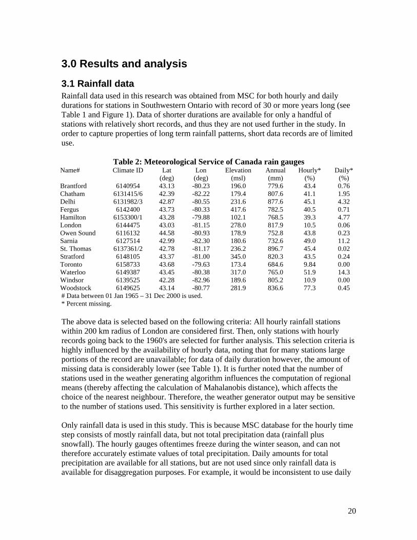
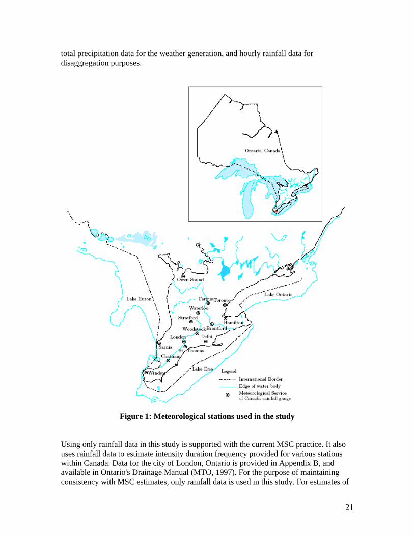
3.1 Rainfall data Rainfall data used in this research was obtained from MSC for both hourly and daily durations for stations in Southwestern Ontario with record of 30 or more years long (see Table 1 and Figure 1). Data of shorter durations are available for only a handful of stations with relatively short records, and thus they are not used further in the study. In order to capture properties of long term rainfall patterns, short data records are of limited use.

Table 2: Meteorological Service of Canada rain gauges Name# Climate ID Lat Lon Elevation Annual Hourly* Daily* (deg) (deg) (msl) (mm) (%) (%) Brantford 6140954 43.13 -80.23 196.0 779.6 43.4 0.76 Chatham 6131415/6 42.39 -82.22 179.4 807.6 41.1 1.95 Delhi 6131982/3 42.87 -80.55 231.6 877.6 45.1 4.32 Fergus 6142400 43.73 -80.33 417.6 782.5 40.5 0.71 Hamilton 6153300/1 43.28 -79.88 102.1 768.5 39.3 4.77 London 6144475 43.03 -81.15 278.0 817.9 10.5 0.06 Owen Sound 6116132 44.58 -80.93 178.9 752.8 43.8 0.23 Sarnia 6127514 42.99 -82.30 180.6 732.6 49.0 11.2 St. Thomas 6137361/2 42.78 -81.17 236.2 896.7 45.4 0.02 Stratford 6148105 43.37 -81.00 345.0 820.3 43.5 0.24 Toronto 6158733 43.68 -79.63 173.4 684.6 9.84 0.00 Waterloo 6149387 43.45 -80.38 317.0 765.0 51.9 14.3 Windsor 6139525 42.28 -82.96 189.6 805.2 10.9 0.00 Woodstock 6149625 43.14 -80.77 281.9 836.6 77.3 0.45 # Data between 01 Jan 1965 – 31 Dec 2000 is used. * Percent missing. The above data is selected based on the following criteria: All hourly rainfall stations within 200 km radius of London are considered first. Then, only stations with hourly records going back to the 1960's are selected for further analysis. This selection criteria is highly influenced by the availability of hourly data, noting that for many stations large portions of the record are unavailable; for data of daily duration however, the amount of missing data is considerably lower (see Table 1). It is further noted that the number of stations used in the weather generating algorithm influences the computation of regional means (thereby affecting the calculation of Mahalanobis distance), which affects the choice of the nearest neighbour. Therefore, the weather generator output may be sensitive to the number of stations used. This sensitivity is further explored in a later section. Only rainfall data is used in this study. This is because MSC database for the hourly time step consists of mostly rainfall data, but not total precipitation data (rainfall plus snowfall). The hourly gauges oftentimes freeze during the winter season, and can not therefore accurately estimate values of total precipitation. Daily amounts for total precipitation are available for all stations, but are not used since only rainfall data is available for disaggregation purposes. For example, it would be inconsistent to use daily

20

total precipitation data for the weather generation, and hourly rainfall data for disaggregation purposes.

Figure 1: Meteorological stations used in the study

Using only rainfall data in this study is supported with the current MSC practice. It also uses rainfall data to estimate intensity duration frequency provided for various stations within Canada. Data for the city of London, Ontario is provided in Appendix B, and available in Ontario's Drainage Manual (MTO, 1997). For the purpose of maintaining consistency with MSC estimates, only rainfall data is used in this study. For estimates of

21

rainfall on snow, the interested reader is referred to Watt et al. (1989) and Wood and Goldt (2004).

3.2 Climate scenarios Two climate change scenarios are selected for this work: scenario B11 (dry) and B21 (wet). These scenarios are chosen as the most appropriate for the study of extremes (especially the study of extreme rainfall). Both are based on the IPCC (2001) scenario story lines B1 and B2. Two scenarios use the information provided by outputs of CSIROM2kb and CCSRNIES global circulation models obtained from the University of Victoria. The B1 storyline depicts a world with rapid global change towards service and information based economies, utilizing reductions of material intensity and use, together with the introduction of clean resource-efficient technologies. The storyline B2 on the other hand emphasizes local solutions to economic, social and environmental well being; it anticipates diverse technological change towards environmental protection and social equity at regional levels. For further description of the scenarios, the reader is referred to Appendix A. The criterion used for selecting scenarios is based on the ability of the scenario to produce a range of possible future climates. The scenario CCSRNIES B21 (wet) is selected as the upper bound of possible future rainfall generated by the global circulation models. Similarly, the scenario CSIROM2kb B11 (dry) is regarded as the lower bound of possible future rainfall magnitude. The two scenarios are therefore selected to show the broad range of climate change impacts on rainfall magnitude. The change fields (described in Section 2.2) for the dry and wet scenario are shown in Table 2. Based on this information, locally observed station data is modified (multiplied by the change fields for each month in the historic record) in order to formulate climate change scenarios appropriate for the City of London at a daily time scale. Development of climate change scenarios in this way considers all available climatic data (local and global) in determining potential future climatic conditions. The wet climate provides conditions where emphasis is placed on increased rainfall magnitude over the next century, while the dry climate emphasizes cooler and drier periods, thus providing information about future drought and drought-like conditions. The wet climate is used specifically to test the region's response to flooding, while the dry climate (examining cooler and drier conditions) can be used in assessment of future low flows. In light of the above discussion, the wet climate therefore represents the upper bound of the range of climate change impacts, while the dry climate scenario corresponds to the lower bound. Note that both wet and dry scenarios are equally likely. However, when dealing with questions regarding the potential increase in rainfall magnitude and frequency, we propose the use of the wet climate scenario (as the most critical). Similarly, if the focus is on low flow conditions, the dry climate is more critical and should therefore be used in the analysis.

22

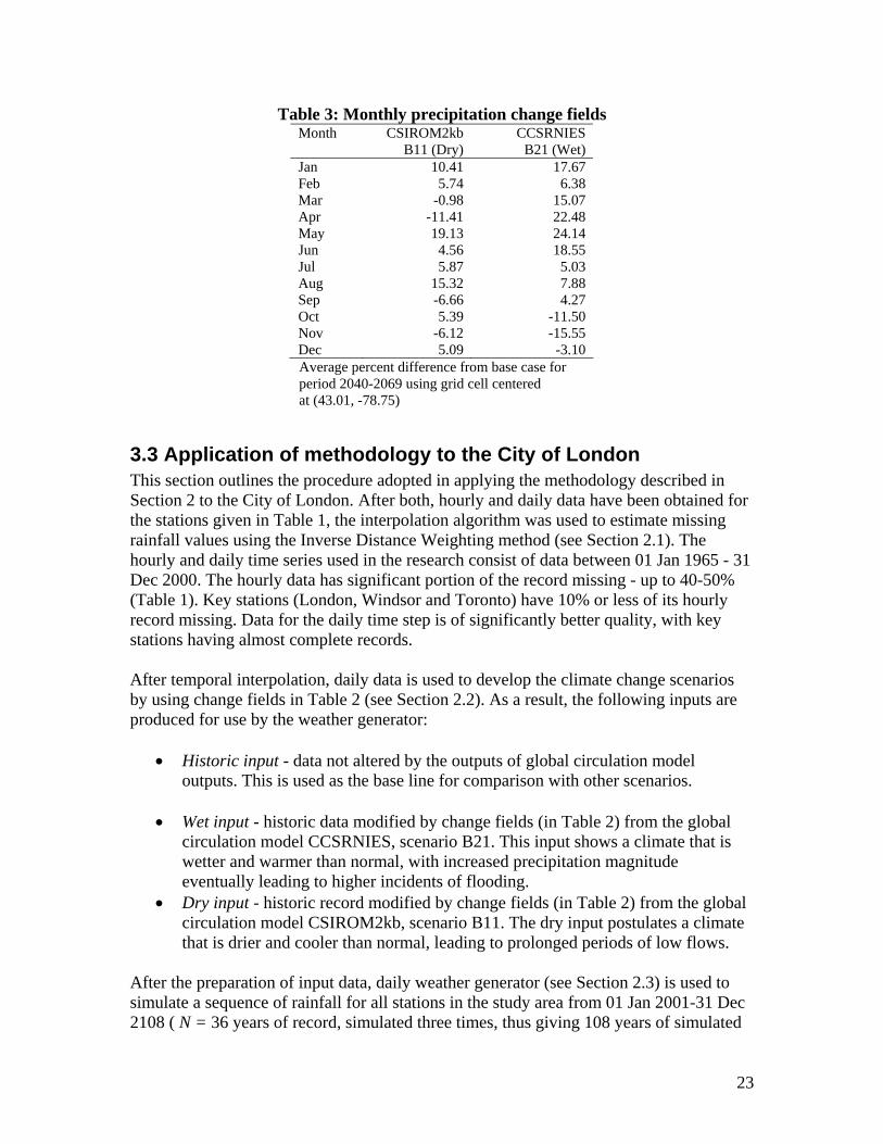
Table 3: Monthly precipitation change fields Month CSIROM2kb CCSRNIES B11 (Dry) B21 (Wet) Jan 10.41 17.67 Feb 5.74 6.38 Mar -0.98 15.07 Apr -11.41 22.48 May 19.13 24.14 Jun 4.56 18.55 Jul 5.87 5.03 Aug 15.32 7.88 Sep -6.66 4.27 Oct 5.39 -11.50 Nov -6.12 -15.55 Dec 5.09 -3.10 Average percent difference from base case for period 2040-2069 using grid cell centered at (43.01, -78.75)

3.3 Application of methodology to the City of London This section outlines the procedure adopted in applying the methodology described in Section 2 to the City of London. After both, hourly and daily data have been obtained for the stations given in Table 1, the interpolation algorithm was used to estimate missing rainfall values using the Inverse Distance Weighting method (see Section 2.1). The hourly and daily time series used in the research consist of data between 01 Jan 1965 - 31 Dec 2000. The hourly data has significant portion of the record missing - up to 40-50% (Table 1). Key stations (London, Windsor and Toronto) have 10% or less of its hourly record missing. Data for the daily time step is of significantly better quality, with key stations having almost complete records. After temporal interpolation, daily data is used to develop the climate change scenarios by using change fields in Table 2 (see Section 2.2). As a result, the following inputs are produced for use by the weather generator:

• Historic input - data not altered by the outputs of global circulation model outputs. This is used as the base line for comparison with other scenarios.

• Wet input - historic data modified by change fields (in Table 2) from the global

circulation model CCSRNIES, scenario B21. This input shows a climate that is wetter and warmer than normal, with increased precipitation magnitude eventually leading to higher incidents of flooding.

• Dry input - historic record modified by change fields (in Table 2) from the global circulation model CSIROM2kb, scenario B11. The dry input postulates a climate that is drier and cooler than normal, leading to prolonged periods of low flows.

After the preparation of input data, daily weather generator (see Section 2.3) is used to simulate a sequence of rainfall for all stations in the study area from 01 Jan 2001-31 Dec 2108 ( N = 36 years of record, simulated three times, thus giving 108 years of simulated

23

output) for each scenario. Such a long record is sufficient for estimating events with return periods as high as 100 years. In the following step, hourly disaggregation algorithm of Section 2.4 is applied to the simulated data, and thus daily output is disaggregated to the hourly time scale. In the disaggregation procedure, the parameter of five hours is used, implying that events

are separated by a period of five hours free of rainfall. Furthermore, the moving window of 60 days is used in the extraction of nearest neighbour events used in the

disaggregation. This value is estimated based on the work of Wey (2006).

sn

hw

Note that historical (unmodified) data is used in the disaggregation procedure, because non-dimensional rainfall mass curves are needed from this data set. Modifying the historic record of hourly data according to the change fields of Table 2 did not significantly affect the resulting temporal distribution. Therefore, historically observed rainfall data is deemed sufficient for disaggregation purposes.

3.4 Verification of weather generator output Following the simulation of daily weather generator and disaggregation of daily to hourly rainfall, statistical tools described in Section 2.5 are applied to test whether the methodology adopted in this study is able to replicate temporal and spacial character of regional rainfall. Figure 2 is shown as output of this analysis. The statistics shown in Figure 2 depict monthly rainfall and lag-1 autocorrelation for the London station, as well as lag-0 crosscorrelation between London and Toronto, and London and Windsor (the stations with least missing hourly data). The presentation of statistics is shown as box and whisker plots, where the bottom and top of the box are showing the 25th and 75th percentile of data, with the median in between. For all cases, historically observed averages are also plotted to identify the ability of the model to represent the structure of temporal and spacial character of rainfall in the area. In all cases, the model adequately replicates the historically observed patterns. A note of caution is offered when reading the results of the monthly rainfall box plot, since its vertical axis extends into a range below zero. This does not mean that the weather generator produces negative rainfall values, or that the plot is showing invalid data. It simply means that extent of the whiskers can be negative (recall the whiskers extend 1.5 times the interquantile range).

24

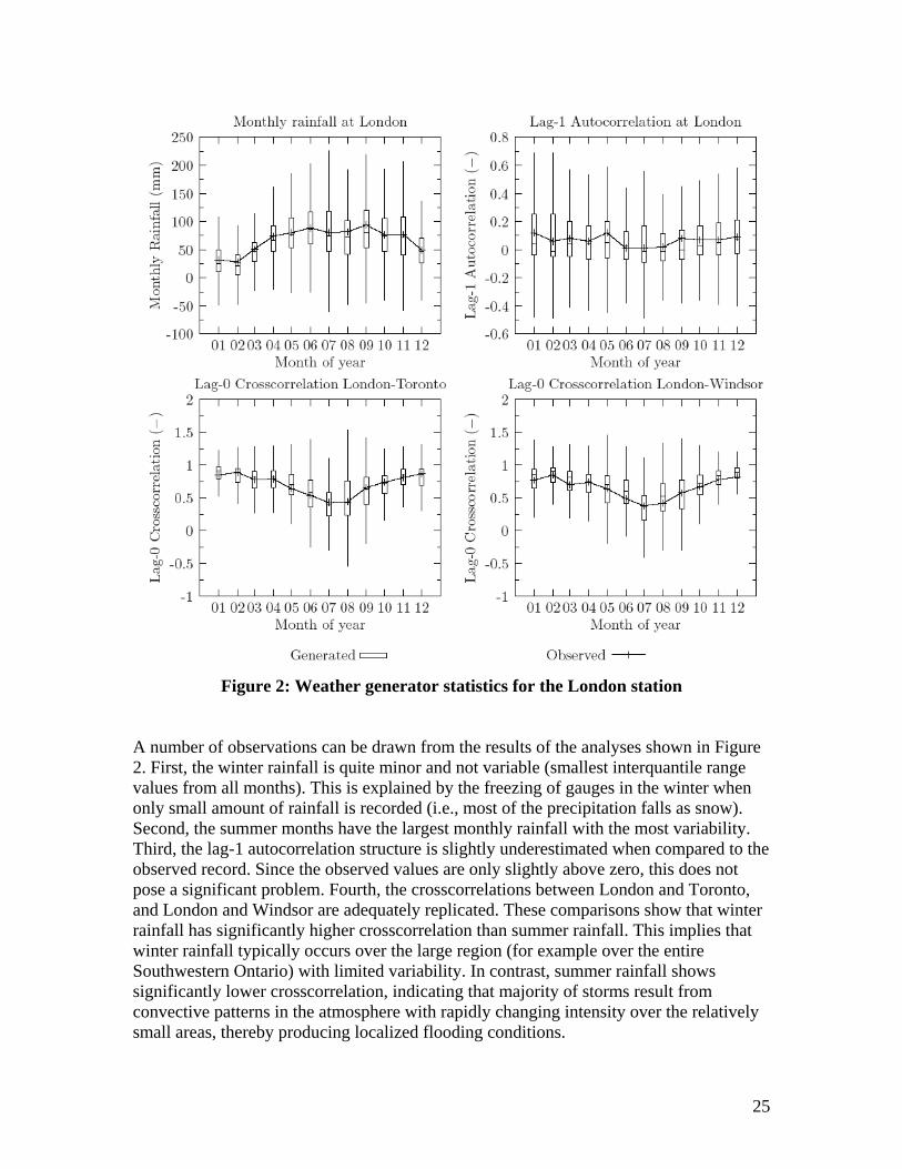
Figure 2: Weather generator statistics for the London station

A number of observations can be drawn from the results of the analyses shown in Figure 2. First, the winter rainfall is quite minor and not variable (smallest interquantile range values from all months). This is explained by the freezing of gauges in the winter when only small amount of rainfall is recorded (i.e., most of the precipitation falls as snow). Second, the summer months have the largest monthly rainfall with the most variability. Third, the lag-1 autocorrelation structure is slightly underestimated when compared to the observed record. Since the observed values are only slightly above zero, this does not pose a significant problem. Fourth, the crosscorrelations between London and Toronto, and London and Windsor are adequately replicated. These comparisons show that winter rainfall has significantly higher crosscorrelation than summer rainfall. This implies that winter rainfall typically occurs over the large region (for example over the entire Southwestern Ontario) with limited variability. In contrast, summer rainfall shows significantly lower crosscorrelation, indicating that majority of storms result from convective patterns in the atmosphere with rapidly changing intensity over the relatively small areas, thereby producing localized flooding conditions.

25

Convective type storms are of most interest for the design of storm water management infrastructure that takes surface runoff away from the streets and safely transports it to storm water management ponds and/or area rivers. Capturing the statistical properties of storms of this kind is achieved through comparison of IDF curves.

3.5 Short duration rainfall under the changing climate The hourly time step rainfall data is used with the procedure of Section 2.6 to develop the intensity duration frequency curves for all climates considered. In order to verify the weather generator and demonstrate adequate reproduction of the historical rainfall even for relatively short durations, an extra weather generator simulation is considered (in addition to simulations of historic, wet and dry climates) in an attempt to replicate the intensity duration frequency data originally produced by the MSC in 2001. This simulation is named historic undisturbed, indicating the removal of the perturbation component responsible for generating unprecedented weather sequences (i.e., removal of Step 10 of the weather generating algorithm). Table 3 summarizes the differences between the input climates, weather generator outputs, as well as a brief description of each simulation considered. Table 4 shows the intensity duration frequency data obtained by undisturbed historic scenario, together with the data produced by MSC in 2001. The intensity duration frequency data acquired from processing output of three weather generator scenarios (historic, wet and dry) is shown in Table 5, from which detailed comparisons can be made. Graphical representation of data presented in Tables 4 and 5 is shown in standard plots, for all scenarios, in Figure 3.

Table 4: Summary of weather generator simulation scenarios Simulation

Output GCM change

fields WG Perturbation

(i.e., Step 10) Description

Historic No Yes Replication of current conditions under no changes in climate

Wet Yes Yes Estimation of future warmer and wetter climate, conditioned by CCSRNIES B21

Dry Yes Yes Estimation of future cooler and drier climate, conditioned by CSIROM2kb B11

Undisturbed Historic

No No Attempt to replicate MSC IDF data

In order to compare the accuracy of the reproduction of the intensity duration frequency data for London, two additional figures are used. The plots of Figure 4 show the comparison between the undisturbed historic, historic and the MSC intensity data for various durations. Through visual inspection, the following is concluded: For rainfall of short duration (1 hr and less) the historic weather generator scenario most closely reproduces the MSC intensity data, for all return periods. For intermediate rainfall

26

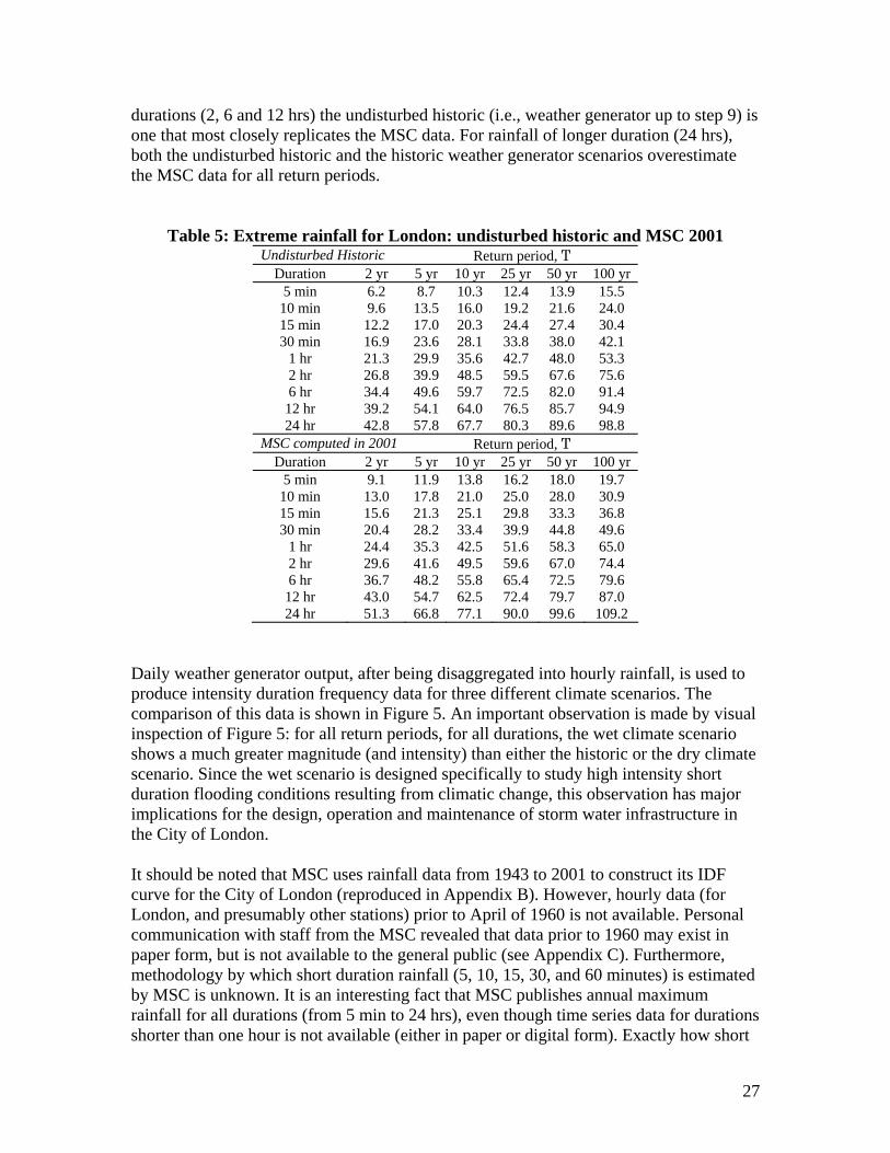
durations (2, 6 and 12 hrs) the undisturbed historic (i.e., weather generator up to step 9) is one that most closely replicates the MSC data. For rainfall of longer duration (24 hrs), both the undisturbed historic and the historic weather generator scenarios overestimate the MSC data for all return periods.

Table 5: Extreme rainfall for London: undisturbed historic and MSC 2001

Undisturbed Historic Return period, T Duration 2 yr 5 yr 10 yr 25 yr 50 yr 100 yr

5 min 6.2 8.7 10.3 12.4 13.9 15.5 10 min 9.6 13.5 16.0 19.2 21.6 24.0 15 min 12.2 17.0 20.3 24.4 27.4 30.4 30 min 16.9 23.6 28.1 33.8 38.0 42.1

1 hr 21.3 29.9 35.6 42.7 48.0 53.3 2 hr 26.8 39.9 48.5 59.5 67.6 75.6 6 hr 34.4 49.6 59.7 72.5 82.0 91.4 12 hr 39.2 54.1 64.0 76.5 85.7 94.9 24 hr 42.8 57.8 67.7 80.3 89.6 98.8

Return period, T MSC computed in 2001 Duration 2 yr 5 yr 10 yr 25 yr 50 yr 100 yr

5 min 9.1 11.9 13.8 16.2 18.0 19.7 10 min 13.0 17.8 21.0 25.0 28.0 30.9 15 min 15.6 21.3 25.1 29.8 33.3 36.8 30 min 20.4 28.2 33.4 39.9 44.8 49.6

1 hr 24.4 35.3 42.5 51.6 58.3 65.0 2 hr 29.6 41.6 49.5 59.6 67.0 74.4 6 hr 36.7 48.2 55.8 65.4 72.5 79.6 12 hr 43.0 54.7 62.5 72.4 79.7 87.0 24 hr 51.3 66.8 77.1 90.0 99.6 109.2

Daily weather generator output, after being disaggregated into hourly rainfall, is used to produce intensity duration frequency data for three different climate scenarios. The comparison of this data is shown in Figure 5. An important observation is made by visual inspection of Figure 5: for all return periods, for all durations, the wet climate scenario shows a much greater magnitude (and intensity) than either the historic or the dry climate scenario. Since the wet scenario is designed specifically to study high intensity short duration flooding conditions resulting from climatic change, this observation has major implications for the design, operation and maintenance of storm water infrastructure in the City of London. It should be noted that MSC uses rainfall data from 1943 to 2001 to construct its IDF curve for the City of London (reproduced in Appendix B). However, hourly data (for London, and presumably other stations) prior to April of 1960 is not available. Personal communication with staff from the MSC revealed that data prior to 1960 may exist in paper form, but is not available to the general public (see Appendix C). Furthermore, methodology by which short duration rainfall (5, 10, 15, 30, and 60 minutes) is estimated by MSC is unknown. It is an interesting fact that MSC publishes annual maximum rainfall for all durations (from 5 min to 24 hrs), even though time series data for durations shorter than one hour is not available (either in paper or digital form). Exactly how short

27

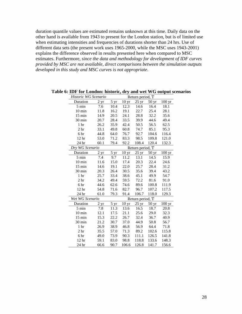
duration quantile values are estimated remains unknown at this time. Daily data on the other hand is available from 1943 to present for the London station, but is of limited use when estimating intensities and frequencies of durations shorter than 24 hrs. Use of different data sets (the present work uses 1965-2000, while the MSC uses 1943-2001) explains the difference observed in results presented here when compared to MSC estimates. Furthermore, since the data and methodology for development of IDF curves provided by MSC are not available, direct comparisons between the simulation outputs developed in this study and MSC curves is not appropriate.

Table 6: IDF for London: historic, dry and wet WG output scenarios Return period, T Historic WG Scenario

Duration 2 yr 5 yr 10 yr 25 yr 50 yr 100 yr 5 min 7.6 10.4 12.3 14.6 16.4 18.1 10 min 11.8 16.2 19.1 22.7 25.4 28.1 15 min 14.9 20.5 24.1 28.8 32.2 35.6 30 min 20.7 28.4 33.5 39.9 44.6 49.4

1 hr 26.2 35.9 42.4 50.5 56.5 62.5 2 hr 33.1 49.8 60.8 74.7 85.1 95.3 6 hr 44.8 64.0 76.7 92.7 104.6 116.4 12 hr 53.0 71.2 83.3 98.5 109.8 121.0 24 hr 60.1 79.4 92.2 108.4 120.4 132.3

Dry WG Scenario Return period, T Duration 2 yr 5 yr 10 yr 25 yr 50 yr 100 yr

5 min 7.4 9.7 11.2 13.1 14.5 15.9 10 min 11.6 15.0 17.4 20.3 22.4 24.6 15 min 14.6 19.1 22.0 25.7 28.4 31.2 30 min 20.3 26.4 30.5 35.6 39.4 43.2

1 hr 25.7 33.4 38.6 45.1 49.9 54.7 2 hr 34.2 49.4 59.5 72.2 81.6 91.0 6 hr 44.6 62.6 74.6 89.6 100.8 111.9 12 hr 54.8 71.6 82.7 96.7 107.2 117.5 24 hr 61.0 79.3 91.4 106.7 118.0 129.3

Wet WG Scenario Return period, T Duration 2 yr 5 yr 10 yr 25 yr 50 yr 100 yr

5 min 7.8 11.3 13.6 16.5 18.7 20.8 10 min 12.1 17.5 21.1 25.6 29.0 32.3 15 min 15.3 22.2 26.7 32.4 36.7 40.9 30 min 21.2 30.7 37.0 44.9 50.8 56.7

1 hr 26.9 38.9 46.8 56.9 64.4 71.8 2 hr 35.5 57.0 71.3 89.2 102.6 115.8 6 hr 49.0 73.9 90.3 111.1 126.5 141.8 12 hr 59.1 83.0 98.8 118.8 133.6 148.3 24 hr 66.6 90.7 106.6 126.8 141.7 156.6

28

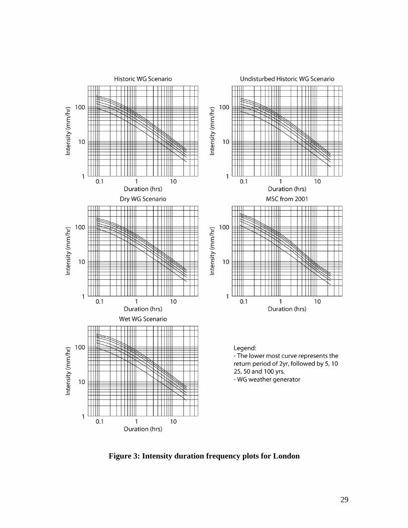
Figure 3: Intensity duration frequency plots for London

29

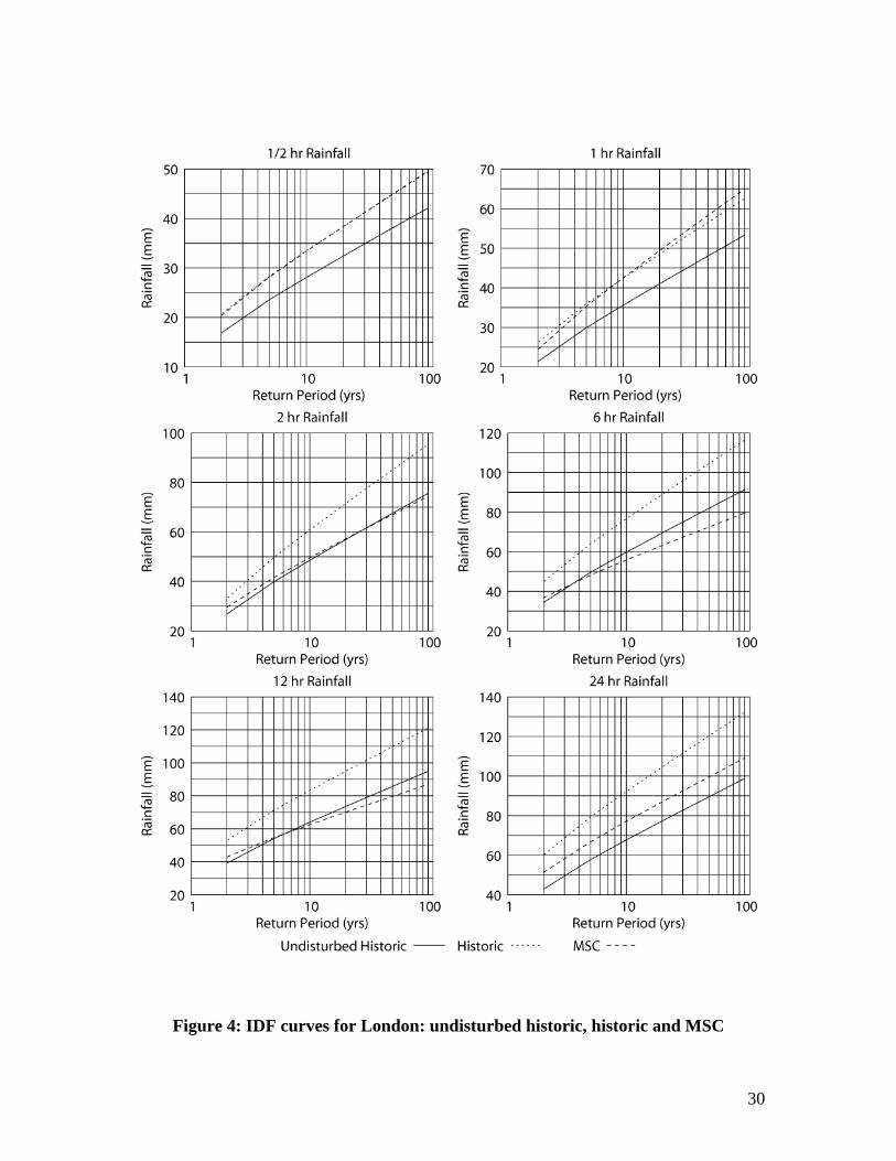
Figure 4: IDF curves for London: undisturbed historic, historic and MSC

30

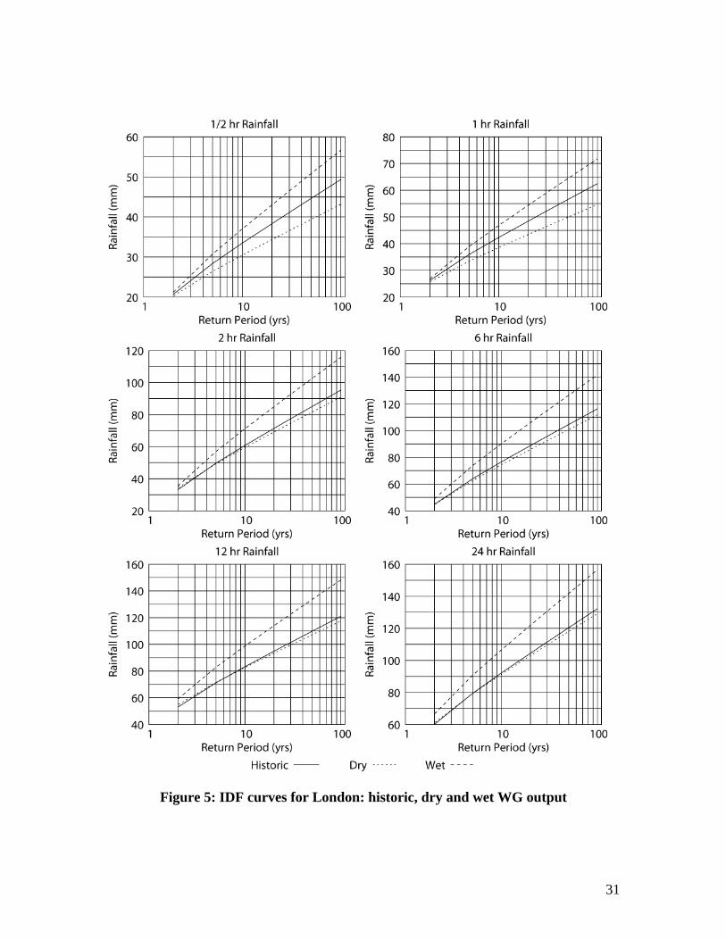
Figure 5: IDF curves for London: historic, dry and wet WG output

31

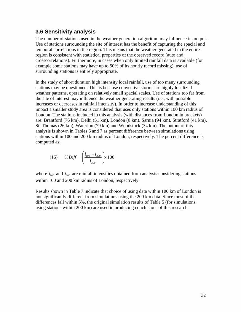
3.6 Sensitivity analysis The number of stations used in the weather generation algorithm may influence its output. Use of stations surrounding the site of interest has the benefit of capturing the spacial and temporal correlations in the region. This means that the weather generated in the entire region is consistent with statistical properties of the observed record (auto and crosscorrelations). Furthermore, in cases when only limited rainfall data is available (for example some stations may have up to 50% of its hourly record missing), use of surrounding stations is entirely appropriate. In the study of short duration high intensity local rainfall, use of too many surrounding stations may be questioned. This is because convective storms are highly localized weather patterns, operating on relatively small spacial scales. Use of stations too far from the site of interest may influence the weather generating results (i.e., with possible increases or decreases in rainfall intensity). In order to increase understanding of this impact a smaller study area is considered that uses only stations within 100 km radius of London. The stations included in this analysis (with distances from London in brackets) are: Brantford (76 km), Delhi (51 km), London (0 km), Sarnia (94 km), Stratford (41 km), St. Thomas (26 km), Waterloo (79 km) and Woodstock (34 km). The output of this analysis is shown in Tables 6 and 7 as percent difference between simulations using stations within 100 and 200 km radius of London, respectively. The percent difference is computed as:

(16) 100%200

200100 ×⎟⎟⎠

⎞⎜⎜⎝

⎛ −=

i

iiDiff

where and are rainfall intensities obtained from analysis considering stations

within 100 and 200 km radius of London, respectively. 100i 200i

Results shown in Table 7 indicate that choice of using data within 100 km of London is not significantly different from simulations using the 200 km data. Since most of the differences fall within 5%, the original simulation results of Table 5 (for simulations using stations within 200 km) are used in producing conclusions of this research.

32

4.0 Conclusions and recommendations

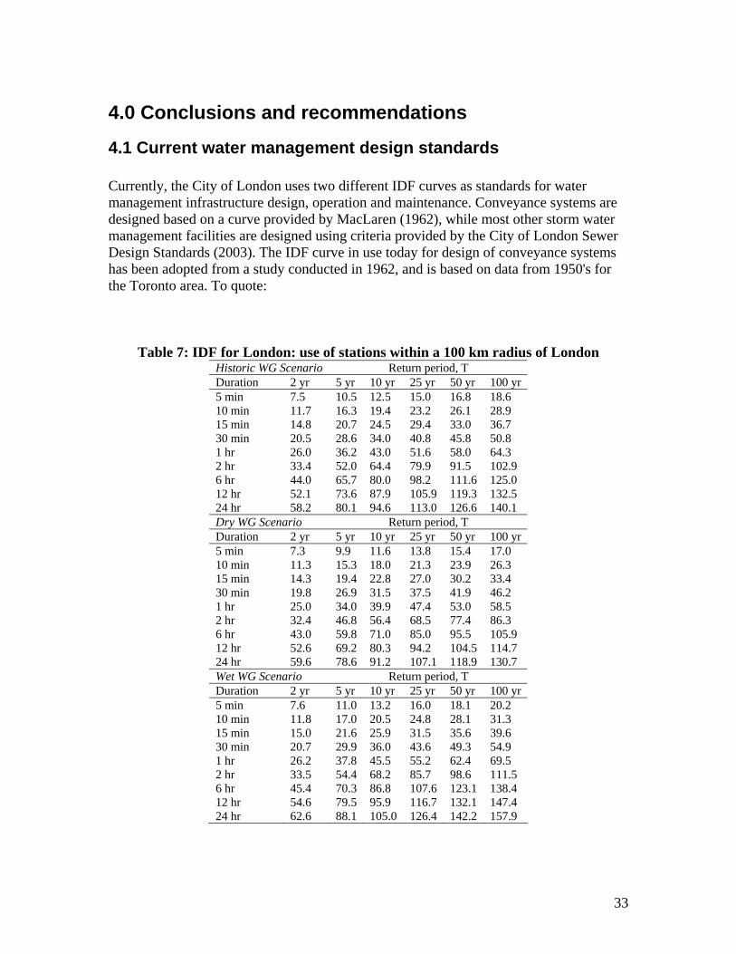
4.1 Current water management design standards Currently, the City of London uses two different IDF curves as standards for water management infrastructure design, operation and maintenance. Conveyance systems are designed based on a curve provided by MacLaren (1962), while most other storm water management facilities are designed using criteria provided by the City of London Sewer Design Standards (2003). The IDF curve in use today for design of conveyance systems has been adopted from a study conducted in 1962, and is based on data from 1950's for the Toronto area. To quote:

Table 7: IDF for London: use of stations within a 100 km radius of London Historic WG Scenario Return period, T Duration 2 yr 5 yr 10 yr 25 yr 50 yr 100 yr 5 min 7.5 10.5 12.5 15.0 16.8 18.6 10 min 11.7 16.3 19.4 23.2 26.1 28.9 15 min 14.8 20.7 24.5 29.4 33.0 36.7 30 min 20.5 28.6 34.0 40.8 45.8 50.8 1 hr 26.0 36.2 43.0 51.6 58.0 64.3 2 hr 33.4 52.0 64.4 79.9 91.5 102.9 6 hr 44.0 65.7 80.0 98.2 111.6 125.0 12 hr 52.1 73.6 87.9 105.9 119.3 132.5 24 hr 58.2 80.1 94.6 113.0 126.6 140.1 Dry WG Scenario Return period, T Duration 2 yr 5 yr 10 yr 25 yr 50 yr 100 yr 5 min 7.3 9.9 11.6 13.8 15.4 17.0 10 min 11.3 15.3 18.0 21.3 23.9 26.3 15 min 14.3 19.4 22.8 27.0 30.2 33.4 30 min 19.8 26.9 31.5 37.5 41.9 46.2 1 hr 25.0 34.0 39.9 47.4 53.0 58.5 2 hr 32.4 46.8 56.4 68.5 77.4 86.3 6 hr 43.0 59.8 71.0 85.0 95.5 105.9 12 hr 52.6 69.2 80.3 94.2 104.5 114.7 24 hr 59.6 78.6 91.2 107.1 118.9 130.7 Wet WG Scenario Return period, T Duration 2 yr 5 yr 10 yr 25 yr 50 yr 100 yr 5 min 7.6 11.0 13.2 16.0 18.1 20.2 10 min 11.8 17.0 20.5 24.8 28.1 31.3 15 min 15.0 21.6 25.9 31.5 35.6 39.6 30 min 20.7 29.9 36.0 43.6 49.3 54.9 1 hr 26.2 37.8 45.5 55.2 62.4 69.5 2 hr 33.5 54.4 68.2 85.7 98.6 111.5 6 hr 45.4 70.3 86.8 107.6 123.1 138.4 12 hr 54.6 79.5 95.9 116.7 132.1 147.4 24 hr 62.6 88.1 105.0 126.4 142.2 157.9

33

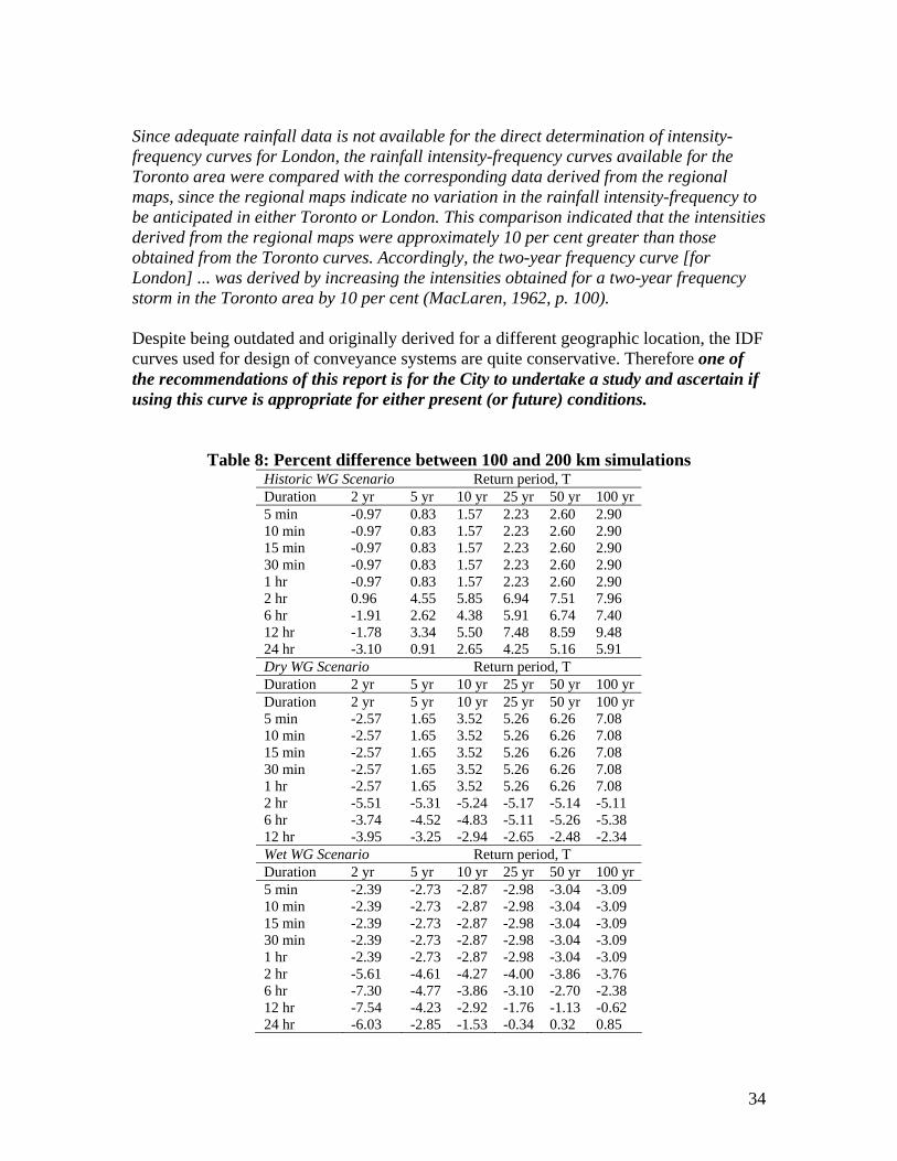
Since adequate rainfall data is not available for the direct determination of intensity-frequency curves for London, the rainfall intensity-frequency curves available for the Toronto area were compared with the corresponding data derived from the regional maps, since the regional maps indicate no variation in the rainfall intensity-frequency to be anticipated in either Toronto or London. This comparison indicated that the intensities derived from the regional maps were approximately 10 per cent greater than those obtained from the Toronto curves. Accordingly, the two-year frequency curve [for London] ... was derived by increasing the intensities obtained for a two-year frequency storm in the Toronto area by 10 per cent (MacLaren, 1962, p. 100). Despite being outdated and originally derived for a different geographic location, the IDF curves used for design of conveyance systems are quite conservative. Therefore one of the recommendations of this report is for the City to undertake a study and ascertain if using this curve is appropriate for either present (or future) conditions.

Table 8: Percent difference between 100 and 200 km simulations Historic WG Scenario Return period, T Duration 2 yr 5 yr 10 yr 25 yr 50 yr 100 yr 5 min -0.97 0.83 1.57 2.23 2.60 2.90 10 min -0.97 0.83 1.57 2.23 2.60 2.90 15 min -0.97 0.83 1.57 2.23 2.60 2.90 30 min -0.97 0.83 1.57 2.23 2.60 2.90 1 hr -0.97 0.83 1.57 2.23 2.60 2.90 2 hr 0.96 4.55 5.85 6.94 7.51 7.96 6 hr -1.91 2.62 4.38 5.91 6.74 7.40 12 hr -1.78 3.34 5.50 7.48 8.59 9.48 24 hr -3.10 0.91 2.65 4.25 5.16 5.91 Dry WG Scenario Return period, T Duration 2 yr 5 yr 10 yr 25 yr 50 yr 100 yr Duration 2 yr 5 yr 10 yr 25 yr 50 yr 100 yr 5 min -2.57 1.65 3.52 5.26 6.26 7.08 10 min -2.57 1.65 3.52 5.26 6.26 7.08 15 min -2.57 1.65 3.52 5.26 6.26 7.08 30 min -2.57 1.65 3.52 5.26 6.26 7.08 1 hr -2.57 1.65 3.52 5.26 6.26 7.08 2 hr -5.51 -5.31 -5.24 -5.17 -5.14 -5.11 6 hr -3.74 -4.52 -4.83 -5.11 -5.26 -5.38 12 hr -3.95 -3.25 -2.94 -2.65 -2.48 -2.34 Wet WG Scenario Return period, T Duration 2 yr 5 yr 10 yr 25 yr 50 yr 100 yr 5 min -2.39 -2.73 -2.87 -2.98 -3.04 -3.09 10 min -2.39 -2.73 -2.87 -2.98 -3.04 -3.09 15 min -2.39 -2.73 -2.87 -2.98 -3.04 -3.09 30 min -2.39 -2.73 -2.87 -2.98 -3.04 -3.09 1 hr -2.39 -2.73 -2.87 -2.98 -3.04 -3.09 2 hr -5.61 -4.61 -4.27 -4.00 -3.86 -3.76 6 hr -7.30 -4.77 -3.86 -3.10 -2.70 -2.38 12 hr -7.54 -4.23 -2.92 -1.76 -1.13 -0.62 24 hr -6.03 -2.85 -1.53 -0.34 0.32 0.85

34

The design of other storm water management infrastructure in the City of London is based on the IDF curve provided by the Atmospheric Environment Service in 1986. (Atmospheric Environment Service was later renamed Meteorological Service of Canada.) The 1986 data was used to fit a 3-hour Chicago rainfall distribution, and thus provide a synthetic distribution for use in design of storm water management facilities in the City of London (City of London Sewer Design Standards, 2003). Since more recent data is available, together with information presented in this report, it is recommended that use of the current standard be reviewed, and updated. This conclusion is supported by the recent work of Markus et al. (2007), where the authors found that older sources of rainfall frequency (those from the 1960's in the Chicago area) consistently produced lower estimates of the design rainfall than those from more recent sources. Markus et al. (2007) also show that larger design rainfall can result in even greater design discharges (due to non-linear nature of the rainfall-runoff process), and thus provide support for the recommendation that current design standards should be reviewed and updated.

4.2 Recommended modifications The rainfall patterns in Southwestern Ontario will most certainly change with the climate change. This report quantifies these changes and their impact on design, operation and maintenance of municipal water management infrastructure (such as roads, bridges, culverts, drains, sewer and conveyance systems, etc). The results are presented in terms of rainfall intensity duration frequency data for the City of London. The analysis performed in this report considered three different scenarios used to evaluate changes in rainfall characteristics for the City of London. Outputs of the study indicate that:

• The rainfall magnitude (as well as intensity) will be different in the future. • The wet climate scenario (recommended for use in storm water management

design standards) reveals significant increase in rainfall magnitude (and intensity) for a range of durations and return periods.

• The increase in rainfall intensity and magnitude has major implications on ways in which current (and future) municipal water management infrastructure is designed, operated, and maintained.

• The design standards and guidelines currently employed by the City of London should be reviewed and/or revised in the lights of the results of this research to reflect the impacts of climatic change.

35

Bibliography Benjamin, J. and Cornell, C. A. (1970). Probability, Statistics and Decision for Civil Engineers. McGraw-Hill, New York. Chow, V. T. (1964). Handbook of applied hydrology. McGraw-Hill Book Company, New York. City of London Sewer Design Standards (2003). City of London, Environmental and Engineering Services Department, London, Ontario, Canada. Coulibaly, P. and Dibike, Y. B. (2004). Downscaling of Global Climate Model Outputs for Flood Frequency Analysis in the Saguenay River System. Final Project Report prepared for the Canadian Climate Change Action Fund, Environment Canada, Hamilton, Ontario, Canada. IPCC (2001). Climate Change 2001: Scientific Basis. Contribution of the Working Group I to the Third Assessment Report of the Intergovernmental Panel on Climate Change. Cambridge University Press, Cambridge, United Kingdom. Kolbert, E. (2006). Field notes from a catastrophe: man, nature, and climate change. Bloomsbury Publishing, New York. Lall, U. and Sharma, A. (1996). “A nearest neighbor bootstrap for time series resampling.” Water Resources Research, 32(3), 679-693. MacLaren, J. F. (1962). Technical Discussion on Sewage and Drainage Works for Areas Annexed in 1961 by the City of London. MacLaren Associates, Toronto, Ontario, Canada. Markus, M., Angel, J. R., Yang, L., and Hejazi, M. I. (2007). “Changing estimates of design precipitation in northeastern illinois: Comparison between different sources and sensitivity analysis.” Journal of Hydrology, accepted for publication. Mehdi, B., Mrena, C., and Douglas, A. (2006). Adapting to climate change: An introduction for Canadian Municipalities. Canadian Climate Impacts and Adaptation Research Network (C-CIARN), http://www.c-ciarn.ca/. MTO (1997). Ministry of Transportation of Ontario Drainage Management Manual. Drainage and Hydrology Section, Transportation Engineering Branch, and Quality Standards Division, Ministry of Transportation of Ontario, Ottawa, Ontario, Canada. Nakicenovic, N. and Swart, R. (2000). IPCC Special Report on Emissions Scenarios, Intergovernmental Panel on Climate Change. Cambridge University Press, Cambridge, United Kingdom.

36

Palmer, R. N., Clancy, E., VanRheenen, N. T., and Wiley, M. W. (2004). The Impacts of Climate Change on The Tualatin River Basin Water Supply: An Investigation into Projected Hydrologic and Management Impacts. Department of Civil and Environmental Engineering, University of Washington, Seattle, Washingtom. Prodanovic, P. and Simonovic, S. P. (2006). “Assessment of water resources risk and vulnerability to changing climatic conditions: Inverse flood risk modelling of the Upper Thames River basin.” Report No. VIII, Department of Civil and Environmental Engineering, The University of Western Ontario, London, Ontario, Canada. Sharif, M. and Burn, D. H. (2004). “Assessment of water resources risk and vulnerability to changing climatic conditions: Development and application of a K-NN weather generating model.” Report No. III, Department of Civil and Environmental Engineering, The University of Western Ontario, London, Ontario, Canada. Sharif, M. and Burn, D. H. (2006a). “Simulating climate change scenarios using an improved K-nearest neighbir model.” Journal of Hydrology, 325, 179-196. Sharif, M. and Burn, D. H. (2006b). “Vulnerability assessment of Upper Thames Basin to climate change scenarios predicted by global circulation models.” EWRI-ASCE International Perspective on Environmental and Water Resources Conference, New Delhi, India. Sharif, M. and Burn, D. H. (2007). “Improved k-nearest neighbor weather generating model.” ASCE Journal of Hydrologic Engineering, 12(1), 42-51. Sharma, A., Tarboton, D., and Lall, U. (1997). “Streamflow simulation: A nonparametric approach.” Water Resources Research, 33(2), 291-308. Southam, C. F., Mills, B. N., Moulton, R. J., and Brown, D. W. (1999). “The potential impact of climate change in Ontario's Grand River Basin: Water supply and demand issues.” Canadian Water Resources Journal, 24(4), 307-330. USACE (2000). Hydrologic Modelling System HEC-HMS, Technical reference manual. United States Army Corps of Engineers, Hydrologic Engineering Center, Davis, California. Watt, W., Lathem, K., Neill, C., Richards, T., and Rousselle, J. (1989). Hydrology of Floods in Canada: A guide to Planning and Design. National Research of Canada, Ottawa, Ontario, Canada. Wey, K. (2006). Temporal disaggregation of daily precipitation data in a changing climate (under preparation). Masters Thesis, Department of Civil Engineering, University of Waterloo, Waterloo, Ontario, Canada.

37

WMO (1994). “Guide to hydrological practice: data acquisition and processing, analysis, forecasting and other applications.” Report No. WMO-No.168, World Meteorological Organization, Geneva, Switzerland. Wojcik, R. and Buishand, T. (2003). “Simulation of 6-hourly rainfall and temperature by two resampling schemes.” Journal of Hydrology, 273, 69-80. Wood, M. and Goldt, R. (2004). Reference Manual for the Use of Precipitation Design Events in The Upper Thames River Watershed. Upper Thames River Conservation Authority, London, Ontario, Canada. Yates, D., Gangopadhyay, S., Rajagopalan, B., and Strzepek, K. (2003). “A technique for generating regional climate scenarios using a nearest-neighbor algorithm.” Water Resources Research, 39(7), SWC7.1-SWC7.15.

38

Appendix

A IPCC Scenarios The following is taken from IPCC (2001) and represent four main families of climate change scenarios. The scenarios used in this report are based on B1 and B2. The A1 storyline and scenario family describes a future world of very rapid economic growth, global population that peaks in mid-century and declines thereafter, and the rapid introduction of new and more efficient technologies. Major underlying themes are convergence among regions, capacity building, and increased cultural and social interactions, with a substantial reduction in regional differences in per capita income. The A1 scenario family develops into three groups that describe alternative directions of technological change in the energy system. The three A1 groups are distinguished by their technological emphasis: fossil intensive (A1FI), non-fossil energy sources (A1T), or a balance across all sources (A1B). The A2 storyline and scenario family describes a very heterogeneous world. The underlying theme is self-reliance and preservation of local identities. Fertility patterns across regions converge very slowly, which results in continuously increasing global population. Economic development is primarily regionally oriented and per capita economic growth and technological change are more fragmented and slower than in other story lines. The B1 storyline and scenario family describes a convergent world with the same global population that peaks in mid- century and declines thereafter, as in the A1 storyline, but with rapid changes in economic structures toward a service and information economy, with reductions in material intensity, and the introduction of clean and resource-efficient technologies. The emphasis is on global solutions to economic, social, and environmental sustainability, including improved equity, but without additional climate initiatives. The B2 storyline and scenario family describes a world in which the emphasis is on local solutions to economic, social, and environmental sustainability. It is a world with continuously increasing global population at a rate lower than A2, intermediate levels of economic development, and less rapid and more diverse technological change than in the B1 and A1 story lines. While the scenario is also oriented toward environmental protection and social equity, it focuses on local and regional levels.

39

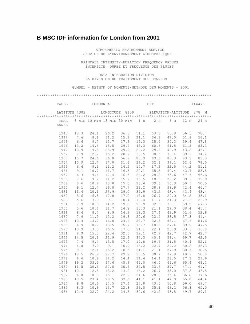
B MSC IDF information for London from 2001

ATMOSPHERIC ENVIRONMENT SERVICE SERVICE DE L"ENVIRONNEMENT ATMOSPHERIQUE RAINFALL INTENSITY-DURATION FREQUENCY VALUES INTENSITE, DUREE ET FREQUENCE DES PLUIES DATA INTEGRATION DIVISION LA DIVISION DU TRAITEMENT DES DONNEES GUMBEL - METHOD OF MOMENTS/METHODE DES MOMENTS - 2001 ******************************************************************************* TABLE 1 LONDON A ONT 6144475 LATITUDE 4302 LONGITUDE 8109 ELEVATION/ALTITUDE 278 M ******************************************************************************* YEAR 5 MIN 10 MIN 15 MIN 30 MIN 1 H 2 H 6 H 12 H 24 H ANNEE 1943 18.3 24.1 26.2 36.3 51.1 53.8 53.8 56.1 78.7 1944 7.6 8.1 11.2 15.2 21.1 34.3 47.0 51.8 56.1 1945 6.6 9.7 12.7 17.3 19.3 25.4 34.3 39.4 47.8 1946 13.2 14.5 15.5 29.7 48.3 60.5 61.5 61.5 83.3 1947 10.9 19.3 23.9 29.2 29.2 29.2 40.9 43.2 46.7 1952 7.9 12.7 15.2 28.7 30.5 30.5 38.4 39.9 74.2 1953 15.7 24.6 36.8 56.9 83.3 83.3 83.3 83.3 83.3 1954 10.9 12.7 17.0 21.6 29.2 32.8 39.1 52.6 78.0 1955 6.6 9.1 11.2 14.2 14.7 17.3 32.5 44.2 51.1 1956 9.1 10.7 11.7 16.8 20.1 35.3 40.4 42.7 53.8 1957 6.3 9.4 12.4 16.5 26.2 28.2 35.6 47.5 55.6 1958 7.6 9.7 11.2 15.7 16.5 18.5 29.2 39.1 39.9 1959 8.6 10.9 13.0 15.5 23.4 39.6 50.3 50.5 50.5 1960 9.1 12.7 16.8 27.7 28.2 38.9 39.9 42.4 46.7 1961 11.4 20.1 23.9 29.0 39.9 43.2 43.4 43.4 43.4 1962 8.6 16.5 17.0 17.0 18.8 26.7 29.0 34.8 35.1 1963 5.6 7.9 9.1 10.4 10.4 11.4 21.3 21.3 23.9 1964 7.9 10.9 14.2 19.0 23.9 32.3 38.1 59.2 67.3 1965 5.6 10.4 11.7 14.2 18.3 21.1 29.0 38.4 43.7 1966 8.4 8.4 8.9 14.2 19.3 27.4 43.9 52.6 52.6 1967 7.9 11.9 12.2 19.3 20.6 22.4 33.5 37.3 41.4 1968 10.4 13.2 16.0 24.6 28.7 32.3 53.1 67.6 84.6 1969 6.9 10.2 13.5 15.7 15.7 18.5 27.4 39.9 47.5 1970 10.9 13.0 16.5 17.0 21.1 22.1 23.9 33.3 36.8 1971 8.9 15.0 22.4 32.5 39.1 42.7 42.7 42.7 42.7 1972 14.5 20.1 22.9 22.9 34.3 40.6 58.4 59.7 62.5 1973 7.4 9.4 13.5 17.0 17.8 19.6 31.5 40.4 52.1 1974 4.8 7.9 9.1 10.9 13.2 22.4 29.2 30.2 35.3 1975 9.1 12.4 15.2 18.5 21.1 21.1 27.9 30.5 30.5 1976 18.5 26.9 27.7 29.2 30.5 30.7 37.8 40.9 50.0 1978 6.6 10.9 14.2 14.4 14.4 14.4 23.5 27.3 29.6 1979 19.2 33.5 37.6 45.9 46.0 46.0 46.6 65.4 68.2 1980 11.5 20.6 27.8 30.6 32.5 32.6 37.7 47.1 61.7 1981 10.1 12.5 13.2 13.2 16.2 26.7 35.0 37.5 43.5 1982 6.8 10.8 15.1 22.2 24.6 28.6 35.4 36.8 37.6 1983 13.5 23.4 29.5 37.6 41.1 41.1 47.0 55.8 64.4 1984 9.8 10.6 14.5 27.4 27.8 43.5 50.8 56.0 69.7 1985 8.3 10.9 13.7 22.8 29.0 35.1 43.2 56.8 65.0 1986 12.4 22.7 24.2 24.5 30.6 42.2 43.8 49.7 89.1

40

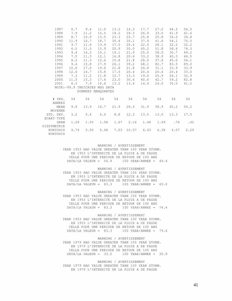
1987 6.7 9.4 11.0 13.2 14.3 17.7 27.2 44.5 56.5 1988 7.9 11.2 15.5 18.2 18.3 26.9 33.0 41.9 61.6 1989 8.7 10.9 13.5 23.3 25.7 25.8 25.8 34.0 34.8 1990 11.9 16.7 18.7 30.4 35.1 37.9 41.6 54.1 75.5 1991 9.7 11.6 13.9 17.5 20.6 22.0 28.1 32.2 32.2 1992 6.5 11.5 15.9 20.9 35.0 45.2 51.8 58.6 76.3 1993 9.4 14.3 15.1 19.1 21.9 25.0 28.5 30.7 49.2 1994 7.5 11.3 12.1 16.8 20.6 33.2 38.9 40.3 46.5 1995 8.2 11.3 12.6 15.8 21.8 28.0 37.8 45.0 56.1 1996 9.4 15.8 17.9 26.1 39.2 68.1 82.7 83.5 89.0 1997 10.6 17.0 19.6 21.8 21.8 24.8 31.1 33.9 33.9 1998 12.6 14.7 15.8 17.6 20.4 20.4 20.4 20.4 33.0 1999 7.3 11.2 11.8 12.7 13.3 19.0 25.9 26.1 32.9 2000 11.5 15.3 17.6 23.0 30.6 40.6 42.7 59.2 82.8 2001 6.3 7.9 10.6 13.2 13.4 14.0 24.0 35.0 41.2 NOTE:-99.9 INDICATES MSG DATA DONNEES MANQUANTES # YRS. 54 54 54 54 54 54 54 54 54 ANNEES MEAN 9.6 13.9 16.7 21.9 26.4 31.9 38.9 45.2 54.2 MOYENNE STD. DEV. 3.2 5.4 6.4 8.8 12.3 13.5 13.0 13.3 17.5 ECART-TYPE SKEW 1.29 1.55 1.58 1.67 2.16 1.48 1.49 .76 .42 DISSYMETRIE KURTOSIS 4.74 5.50 5.48 7.03 10.57 6.43 6.38 4.07 2.29 KURTOSIS WARNING / AVERTISSEMENT YEAR 1953 HAD VALUE GREATER THAN 100 YEAR STORM. EN 1953 L"INTENSITE DE LA PLUIE A DE PASSE CELLE POUR UNE PERIODE DE RETOUR DE 100 ANS DATA/LA VALEUR = 56.9 100 YEAR/ANNEE = 49.6 WARNING / AVERTISSEMENT YEAR 1953 HAD VALUE GREATER THAN 100 YEAR STORM. EN 1953 L"INTENSITE DE LA PLUIE A DE PASSE CELLE POUR UNE PERIODE DE RETOUR DE 100 ANS DATA/LA VALEUR = 83.3 100 YEAR/ANNEE = 65.0 WARNING / AVERTISSEMENT YEAR 1953 HAD VALUE GREATER THAN 100 YEAR STORM. EN 1953 L"INTENSITE DE LA PLUIE A DE PASSE CELLE POUR UNE PERIODE DE RETOUR DE 100 ANS DATA/LA VALEUR = 83.3 100 YEAR/ANNEE = 74.4 WARNING / AVERTISSEMENT YEAR 1953 HAD VALUE GREATER THAN 100 YEAR STORM. EN 1953 L"INTENSITE DE LA PLUIE A DE PASSE CELLE POUR UNE PERIODE DE RETOUR DE 100 ANS DATA/LA VALEUR = 83.3 100 YEAR/ANNEE = 79.6 WARNING / AVERTISSEMENT YEAR 1979 HAD VALUE GREATER THAN 100 YEAR STORM. EN 1979 L"INTENSITE DE LA PLUIE A DE PASSE CELLE POUR UNE PERIODE DE RETOUR DE 100 ANS DATA/LA VALEUR = 33.5 100 YEAR/ANNEE = 30.9 WARNING / AVERTISSEMENT YEAR 1979 HAD VALUE GREATER THAN 100 YEAR STORM. EN 1979 L"INTENSITE DE LA PLUIE A DE PASSE

41

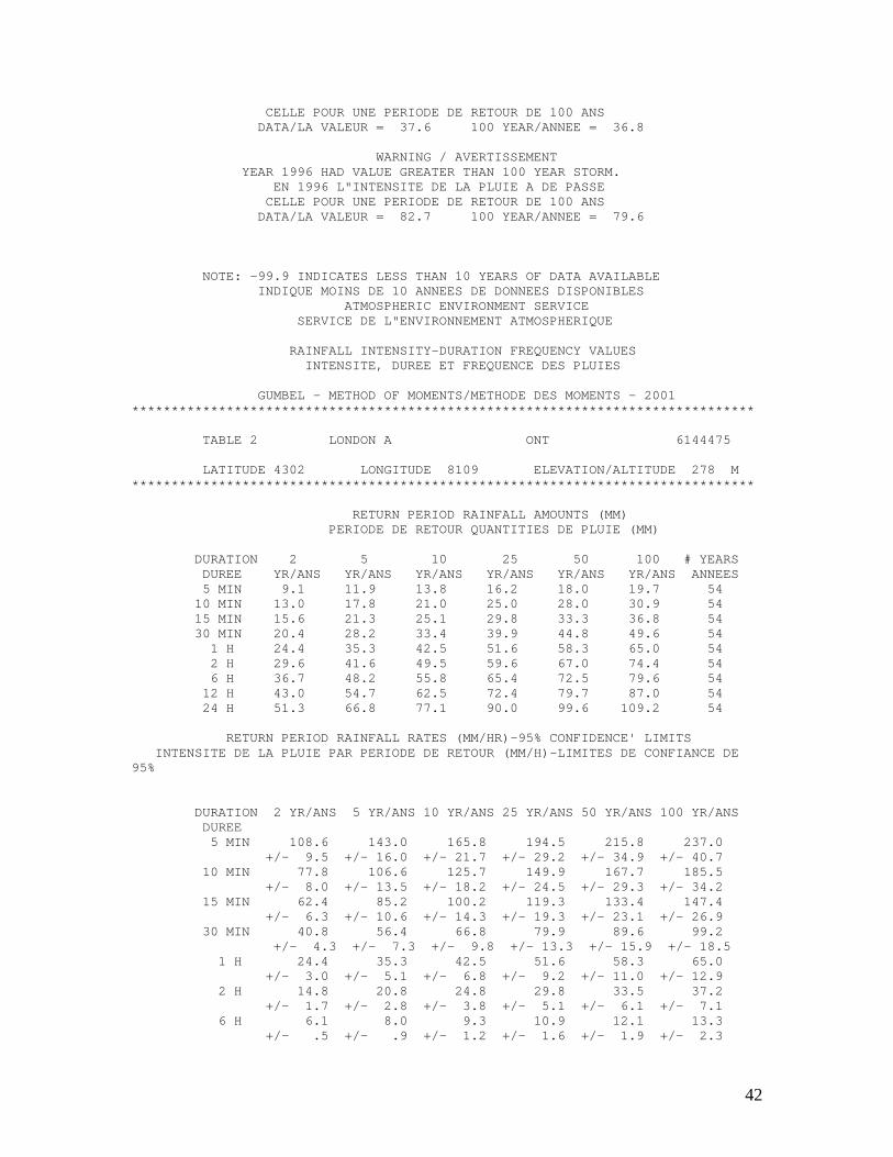
CELLE POUR UNE PERIODE DE RETOUR DE 100 ANS DATA/LA VALEUR = 37.6 100 YEAR/ANNEE = 36.8 WARNING / AVERTISSEMENT YEAR 1996 HAD VALUE GREATER THAN 100 YEAR STORM. EN 1996 L"INTENSITE DE LA PLUIE A DE PASSE CELLE POUR UNE PERIODE DE RETOUR DE 100 ANS DATA/LA VALEUR = 82.7 100 YEAR/ANNEE = 79.6 NOTE: -99.9 INDICATES LESS THAN 10 YEARS OF DATA AVAILABLE INDIQUE MOINS DE 10 ANNEES DE DONNEES DISPONIBLES ATMOSPHERIC ENVIRONMENT SERVICE SERVICE DE L"ENVIRONNEMENT ATMOSPHERIQUE RAINFALL INTENSITY-DURATION FREQUENCY VALUES INTENSITE, DUREE ET FREQUENCE DES PLUIES GUMBEL - METHOD OF MOMENTS/METHODE DES MOMENTS - 2001 ******************************************************************************* TABLE 2 LONDON A ONT 6144475 LATITUDE 4302 LONGITUDE 8109 ELEVATION/ALTITUDE 278 M ******************************************************************************* RETURN PERIOD RAINFALL AMOUNTS (MM) PERIODE DE RETOUR QUANTITIES DE PLUIE (MM) DURATION 2 5 10 25 50 100 # YEARS DUREE YR/ANS YR/ANS YR/ANS YR/ANS YR/ANS YR/ANS ANNEES 5 MIN 9.1 11.9 13.8 16.2 18.0 19.7 54 10 MIN 13.0 17.8 21.0 25.0 28.0 30.9 54 15 MIN 15.6 21.3 25.1 29.8 33.3 36.8 54 30 MIN 20.4 28.2 33.4 39.9 44.8 49.6 54 1 H 24.4 35.3 42.5 51.6 58.3 65.0 54 2 H 29.6 41.6 49.5 59.6 67.0 74.4 54 6 H 36.7 48.2 55.8 65.4 72.5 79.6 54 12 H 43.0 54.7 62.5 72.4 79.7 87.0 54 24 H 51.3 66.8 77.1 90.0 99.6 109.2 54 RETURN PERIOD RAINFALL RATES (MM/HR)-95% CONFIDENCE' LIMITS INTENSITE DE LA PLUIE PAR PERIODE DE RETOUR (MM/H)-LIMITES DE CONFIANCE DE 95% DURATION 2 YR/ANS 5 YR/ANS 10 YR/ANS 25 YR/ANS 50 YR/ANS 100 YR/ANS DUREE 5 MIN 108.6 143.0 165.8 194.5 215.8 237.0 +/- 9.5 +/- 16.0 +/- 21.7 +/- 29.2 +/- 34.9 +/- 40.7 10 MIN 77.8 106.6 125.7 149.9 167.7 185.5 +/- 8.0 +/- 13.5 +/- 18.2 +/- 24.5 +/- 29.3 +/- 34.2 15 MIN 62.4 85.2 100.2 119.3 133.4 147.4 +/- 6.3 +/- 10.6 +/- 14.3 +/- 19.3 +/- 23.1 +/- 26.9 30 MIN 40.8 56.4 66.8 79.9 89.6 99.2 +/- 4.3 +/- 7.3 +/- 9.8 +/- 13.3 +/- 15.9 +/- 18.5 1 H 24.4 35.3 42.5 51.6 58.3 65.0 +/- 3.0 +/- 5.1 +/- 6.8 +/- 9.2 +/- 11.0 +/- 12.9 2 H 14.8 20.8 24.8 29.8 33.5 37.2 +/- 1.7 +/- 2.8 +/- 3.8 +/- 5.1 +/- 6.1 +/- 7.1 6 H 6.1 8.0 9.3 10.9 12.1 13.3 +/- .5 +/- .9 +/- 1.2 +/- 1.6 +/- 1.9 +/- 2.3

42

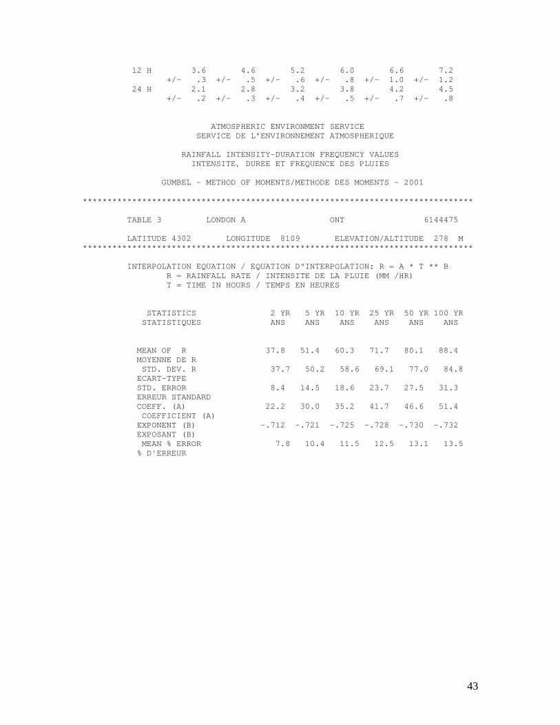
12 H 3.6 4.6 5.2 6.0 6.6 7.2 +/- .3 +/- .5 +/- .6 +/- .8 +/- 1.0 +/- 1.2 24 H 2.1 2.8 3.2 3.8 4.2 4.5 +/- .2 +/- .3 +/- .4 +/- .5 +/- .7 +/- .8 ATMOSPHERIC ENVIRONMENT SERVICE SERVICE DE L"ENVIRONNEMENT ATMOSPHERIQUE RAINFALL INTENSITY-DURATION FREQUENCY VALUES INTENSITE, DUREE ET FREQUENCE DES PLUIES GUMBEL - METHOD OF MOMENTS/METHODE DES MOMENTS - 2001 ******************************************************************************* TABLE 3 LONDON A ONT 6144475 LATITUDE 4302 LONGITUDE 8109 ELEVATION/ALTITUDE 278 M ******************************************************************************* INTERPOLATION EQUATION / EQUATION D"INTERPOLATION: R = A * T ** B R = RAINFALL RATE / INTENSITE DE LA PLUIE (MM /HR) T = TIME IN HOURS / TEMPS EN HEURES STATISTICS 2 YR 5 YR 10 YR 25 YR 50 YR 100 YR STATISTIQUES ANS ANS ANS ANS ANS ANS MEAN OF R 37.8 51.4 60.3 71.7 80.1 88.4 MOYENNE DE R STD. DEV. R 37.7 50.2 58.6 69.1 77.0 84.8 ECART-TYPE STD. ERROR 8.4 14.5 18.6 23.7 27.5 31.3 ERREUR STANDARD COEFF. (A) 22.2 30.0 35.2 41.7 46.6 51.4 COEFFICIENT (A) EXPONENT (B) -.712 -.721 -.725 -.728 -.730 -.732 EXPOSANT (B) MEAN % ERROR 7.8 10.4 11.5 12.5 13.1 13.5 % D'ERREUR

43

C Communication with MSC Original message from P. Prodanovic: From: Predrag Prodanovic [mailto:pprodano@uwo.ca] Sent: October 30, 2007 9:35 AM To: Radecki,Sandy [Ontario] Subject: Climate data availability and a question Hello Sandy, Few months ago I have obtained hourly data from what I understand is your TBRG database. The person I have been dealing with was Maria Petrou. This time I have two questions, and I think you might be able to help me. The hourly data I obtained (for stations within a 200 km radius of London, Ontario) included data up to October 2002. However, our client wishes that we use data up to 2007. Do you think this is possible? Part of our study is looking at ways in which intensity duration frequency of rainfall will change as the climate changes. Atmospheric Environment Service used to provide such curves (the latest one was issued in 2001) for many places around Canada. I am attaching one of their documents (for London, Ontario) that summarizes this data. For example, hourly data for the London station is available from 1960 (this is what I was able to obtained from Maria), yet the attached document shows an annual extreme of the hourly data from as early as 1943. The same logic is applied to estimates by AES of 5, 10, 15, and 30 min rainfall; this data is not available, and yet the estimates are made. The question that I have is the following: By which means was AES able to estimate rainfall quantiles when the time series data is not available? If you are not the right person to answer these questions, may I kindly ask to suggest someone who you think might be able to help. Thank you in advance, Predrag Prodanovic

44

Response from Sandy Radecki, Meteorological Service of Canada: Date: Tue, 30 Oct 2007 12:50:11 -0400 From: Ontario Climate Centre mailto: Ontario.Climate.Centre@ec.gc.ca To: Predrag Prodanovic mailto: pprodano@uwo.ca Subject: RE: Climate data availability and a question The hourly rainfall for Ontario has been updated to include data only to 2003. The more recent information still has to be processed through quality control. It is unknown when this additional data will become available to the archive - as we are short staffed in our office. The values before 1960 must have been part of an alternative archive that may have been on paper only. When the digital archive was first established there were some decisions made as to how much of the previous record would be archived digitally. The decision to put only data back to 1960 for London must have been at that time. Sandy Radecki Ontario Climate Centre 4905 Dufferin Street Toronto, Ontario M3H 5T4 fax 416-739-4521 email ontario.climate@ec.gc.ca For climate data try www.climate.weatheroffice.ec.gc.ca For general enquiries 1-900-565-1111 charge of $2.99 per minute

45

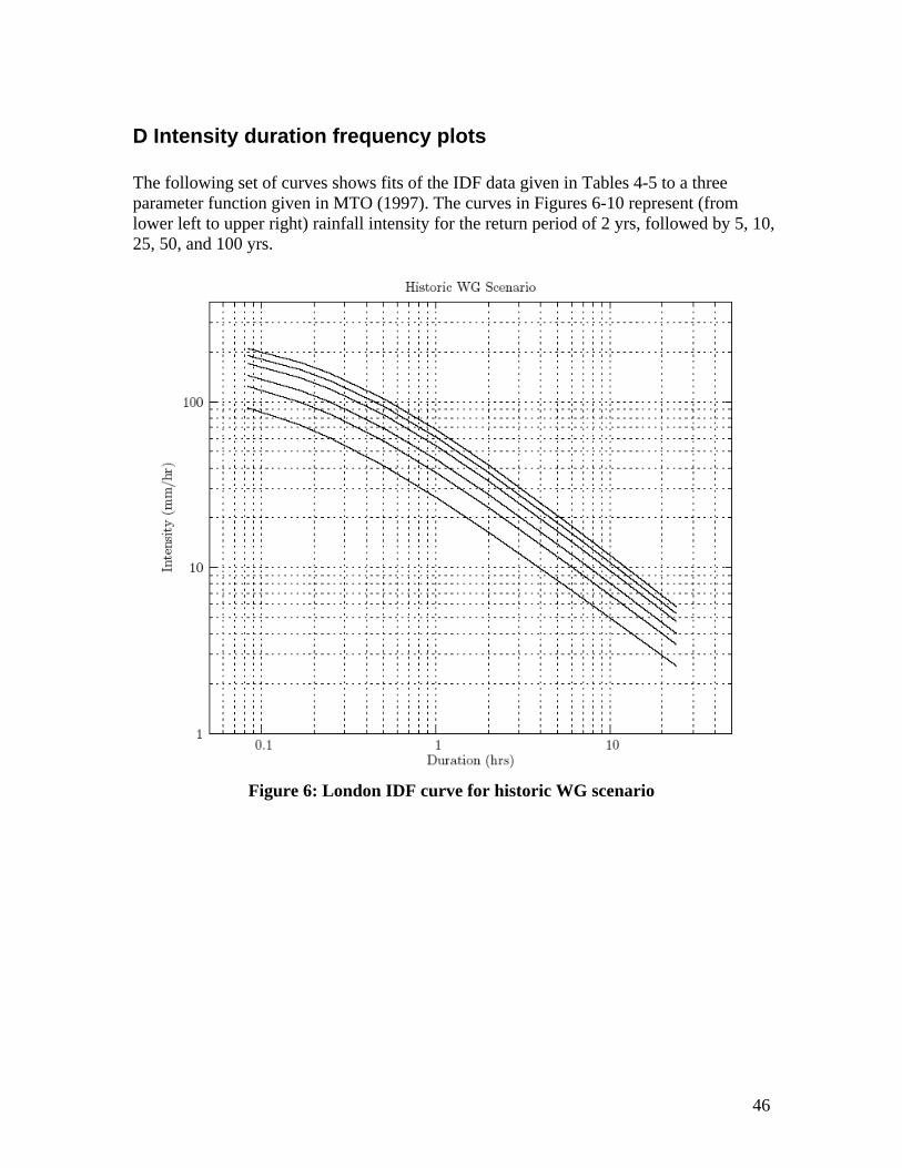
D Intensity duration frequency plots The following set of curves shows fits of the IDF data given in Tables 4-5 to a three parameter function given in MTO (1997). The curves in Figures 6-10 represent (from lower left to upper right) rainfall intensity for the return period of 2 yrs, followed by 5, 10, 25, 50, and 100 yrs.

Figure 6: London IDF curve for historic WG scenario

46

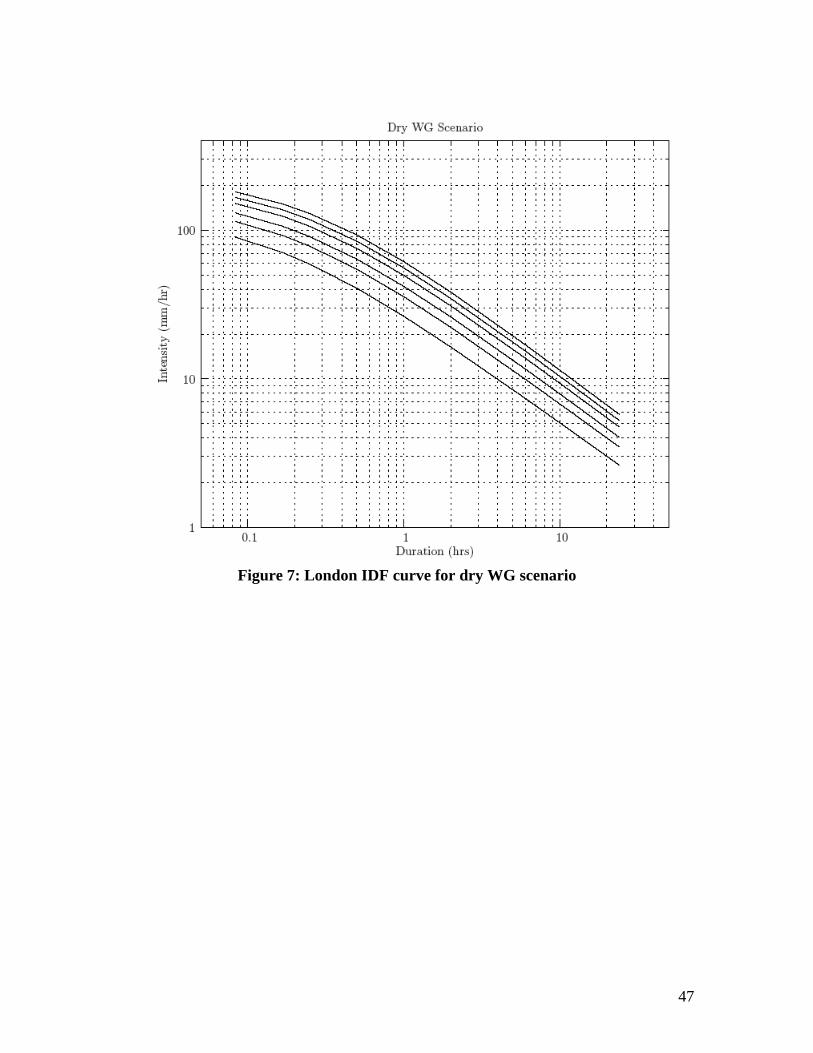
Figure 7: London IDF curve for dry WG scenario

47

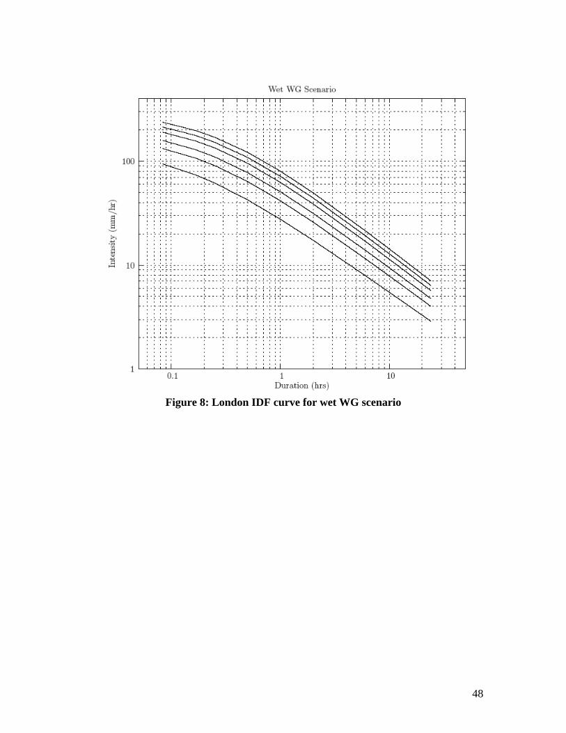
Figure 8: London IDF curve for wet WG scenario

48

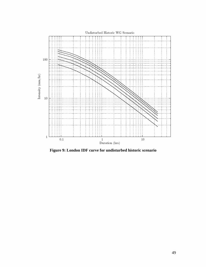
Figure 9: London IDF curve for undisturbed historic scenario

49

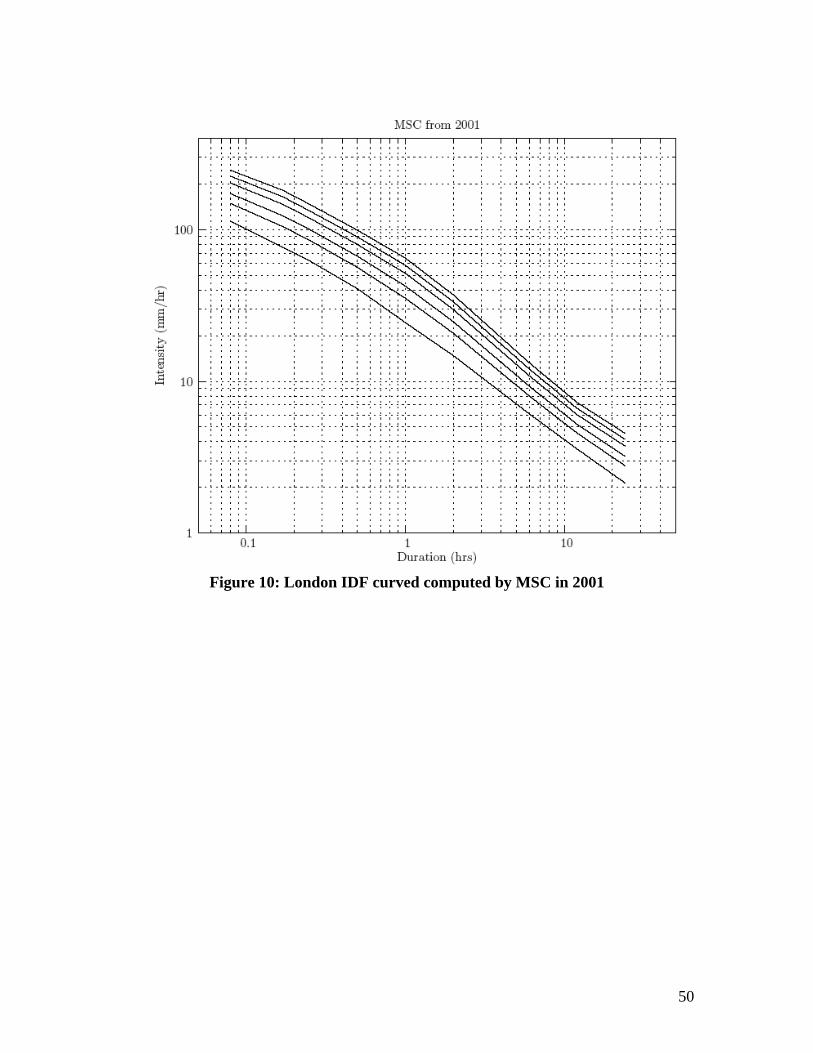
Figure 10: London IDF curved computed by MSC in 2001

50