________________________________________________________________________

U.S. Department of the Interior U.S. Geological Survey

DOCUMENTATION OF REVISIONS TO THE REGIONAL AQUIFER SYSTEM ANALYSIS MODEL OF THE NEW JERSEY COASTAL PLAIN

Water-Resources Investigations Report 03-4268

In cooperation with the NEW JERSEY DEPARTMENT OF ENVIRONMENTAL PROTECTION

________________________________________________________________________

DOCUMENTATION OF REVISIONS TO THE REGIONAL AQUIFER SYSTEM ANALYSIS MODEL OF THE NEW JERSEY COASTAL PLAIN

By Lois M. Voronin

U.S. Geological Survey

Water-Resources Investigations Report 03-4268

In cooperation with the NEW JERSEY DEPARTMENT OF ENVIRONMENTAL PROTECTION

U.S. DEPARTMENT OF THE INTERIOR GALE A. NORTON, Secretary

U.S. GEOLOGICAL SURVEY

Charles G. Groat, Director

For additional information Copies of this report can be write to: purchased from:

District Chief U.S. Geological Survey U.S. Geological Survey Mountain View Office Park Branch of Information Services 810 Bear Tavern Road Box 25286 West Trenton, NJ 08628 Denver, CO 80225-0286

iii

Contents

Abstract. . . . . . . . . . . . . . . . . . . . . . . . . . . . . . . . . . . . . . . . . . . . . . . . . . . . . . . . . . . . . . . . . . . . . . . . . . . . . . . . . . . . . . . . . . . . . . . . . . . . . . . . . . . . . . . . . . . . . . . . . . .1Introduction . . . . . . . . . . . . . . . . . . . . . . . . . . . . . . . . . . . . . . . . . . . . . . . . . . . . . . . . . . . . . . . . . . . . . . . . . . . . . . . . . . . . . . . . . . . . . . . . . . . . . . . . . . . . . . . . . . . . . . 1

Purpose and scope . . . . . . . . . . . . . . . . . . . . . . . . . . . . . . . . . . . . . . . . . . . . . . . . . . . . . . . . . . . . . . . . . . . . . . . . . . . . . . . . . . . . . . . . . . . . . . . . . . . . . . . . 3Location and extent of study area . . . . . . . . . . . . . . . . . . . . . . . . . . . . . . . . . . . . . . . . . . . . . . . . . . . . . . . . . . . . . . . . . . . . . . . . . . . . . . . . . . . . . . . . . . .3Previous investigations. . . . . . . . . . . . . . . . . . . . . . . . . . . . . . . . . . . . . . . . . . . . . . . . . . . . . . . . . . . . . . . . . . . . . . . . . . . . . . . . . . . . . . . . . . . . . . . . . . . . . 3Conceptual hydrogeologic model. . . . . . . . . . . . . . . . . . . . . . . . . . . . . . . . . . . . . . . . . . . . . . . . . . . . . . . . . . . . . . . . . . . . . . . . . . . . . . . . . . . . . . . . . . . .3

Hydrogeologic framework. . . . . . . . . . . . . . . . . . . . . . . . . . . . . . . . . . . . . . . . . . . . . . . . . . . . . . . . . . . . . . . . . . . . . . . . . . . . . . . . . . . . . . . . . . . . 3Ground-water-flow system . . . . . . . . . . . . . . . . . . . . . . . . . . . . . . . . . . . . . . . . . . . . . . . . . . . . . . . . . . . . . . . . . . . . . . . . . . . . . . . . . . . . . . . . . . . 3

Original and revised model designs. . . . . . . . . . . . . . . . . . . . . . . . . . . . . . . . . . . . . . . . . . . . . . . . . . . . . . . . . . . . . . . . . . . . . . . . . . . . . . . . . . . . . . . . . . . . . . . 4Model approach . . . . . . . . . . . . . . . . . . . . . . . . . . . . . . . . . . . . . . . . . . . . . . . . . . . . . . . . . . . . . . . . . . . . . . . . . . . . . . . . . . . . . . . . . . . . . . . . . . . . . . . . . . . 4Grid design. . . . . . . . . . . . . . . . . . . . . . . . . . . . . . . . . . . . . . . . . . . . . . . . . . . . . . . . . . . . . . . . . . . . . . . . . . . . . . . . . . . . . . . . . . . . . . . . . . . . . . . . . . . . . . . . . .4Ground-water withdrawals. . . . . . . . . . . . . . . . . . . . . . . . . . . . . . . . . . . . . . . . . . . . . . . . . . . . . . . . . . . . . . . . . . . . . . . . . . . . . . . . . . . . . . . . . . . . . . . . . 4Lateral and lower boundary conditions . . . . . . . . . . . . . . . . . . . . . . . . . . . . . . . . . . . . . . . . . . . . . . . . . . . . . . . . . . . . . . . . . . . . . . . . . . . . . . . . . . . . . .9Upper boundary conditions. . . . . . . . . . . . . . . . . . . . . . . . . . . . . . . . . . . . . . . . . . . . . . . . . . . . . . . . . . . . . . . . . . . . . . . . . . . . . . . . . . . . . . . . . . . . . . . . . 9

Streams . . . . . . . . . . . . . . . . . . . . . . . . . . . . . . . . . . . . . . . . . . . . . . . . . . . . . . . . . . . . . . . . . . . . . . . . . . . . . . . . . . . . . . . . . . . . . . . . . . . . . . . . . . . . . . 9Recharge. . . . . . . . . . . . . . . . . . . . . . . . . . . . . . . . . . . . . . . . . . . . . . . . . . . . . . . . . . . . . . . . . . . . . . . . . . . . . . . . . . . . . . . . . . . . . . . . . . . . . . . . . . . . 13

Model calibration. . . . . . . . . . . . . . . . . . . . . . . . . . . . . . . . . . . . . . . . . . . . . . . . . . . . . . . . . . . . . . . . . . . . . . . . . . . . . . . . . . . . . . . . . . . . . . . . . . . . . . . . . . . . . . . . 13Revisions to model input data. . . . . . . . . . . . . . . . . . . . . . . . . . . . . . . . . . . . . . . . . . . . . . . . . . . . . . . . . . . . . . . . . . . . . . . . . . . . . . . . . . . . . . . . . . . . . . 13

Recharge. . . . . . . . . . . . . . . . . . . . . . . . . . . . . . . . . . . . . . . . . . . . . . . . . . . . . . . . . . . . . . . . . . . . . . . . . . . . . . . . . . . . . . . . . . . . . . . . . . . . . . . . . . . . 13Vertical leakance . . . . . . . . . . . . . . . . . . . . . . . . . . . . . . . . . . . . . . . . . . . . . . . . . . . . . . . . . . . . . . . . . . . . . . . . . . . . . . . . . . . . . . . . . . . . . . . . . . . . 13Storage coefficient . . . . . . . . . . . . . . . . . . . . . . . . . . . . . . . . . . . . . . . . . . . . . . . . . . . . . . . . . . . . . . . . . . . . . . . . . . . . . . . . . . . . . . . . . . . . . . . . . . 17Boundary fluxes . . . . . . . . . . . . . . . . . . . . . . . . . . . . . . . . . . . . . . . . . . . . . . . . . . . . . . . . . . . . . . . . . . . . . . . . . . . . . . . . . . . . . . . . . . . . . . . . . . . . . 18

Simulated potentiometric surfaces . . . . . . . . . . . . . . . . . . . . . . . . . . . . . . . . . . . . . . . . . . . . . . . . . . . . . . . . . . . . . . . . . . . . . . . . . . . . . . . . . . . . . . . . 181978 ground-water-flow conditions . . . . . . . . . . . . . . . . . . . . . . . . . . . . . . . . . . . . . . . . . . . . . . . . . . . . . . . . . . . . . . . . . . . . . . . . . . . . . . . . . . 181998 ground-water-flow conditions . . . . . . . . . . . . . . . . . . . . . . . . . . . . . . . . . . . . . . . . . . . . . . . . . . . . . . . . . . . . . . . . . . . . . . . . . . . . . . . . . . 18

Simulated and measured water-level hydrographs . . . . . . . . . . . . . . . . . . . . . . . . . . . . . . . . . . . . . . . . . . . . . . . . . . . . . . . . . . . . . . . . . . . . . . . . 31Base flow . . . . . . . . . . . . . . . . . . . . . . . . . . . . . . . . . . . . . . . . . . . . . . . . . . . . . . . . . . . . . . . . . . . . . . . . . . . . . . . . . . . . . . . . . . . . . . . . . . . . . . . . . . . . . . . . . 31Model limitations. . . . . . . . . . . . . . . . . . . . . . . . . . . . . . . . . . . . . . . . . . . . . . . . . . . . . . . . . . . . . . . . . . . . . . . . . . . . . . . . . . . . . . . . . . . . . . . . . . . . . . . . . . 31

Summary. . . . . . . . . . . . . . . . . . . . . . . . . . . . . . . . . . . . . . . . . . . . . . . . . . . . . . . . . . . . . . . . . . . . . . . . . . . . . . . . . . . . . . . . . . . . . . . . . . . . . . . . . . . . . . . . . . . . . . . . 48References cited . . . . . . . . . . . . . . . . . . . . . . . . . . . . . . . . . . . . . . . . . . . . . . . . . . . . . . . . . . . . . . . . . . . . . . . . . . . . . . . . . . . . . . . . . . . . . . . . . . . . . . . . . . . . . . . . 48

Plate

[In pocket] 1. Map showing finite-difference grid and generalized lateral boundaries of the original and revised Regional Aquifer System

Analysis models

CD-ROM

[In pocket] 1. Read me file and model files.

iv

Figures

1. Map showing location of study area and Critical Water Supply areas 1 and 2 in New Jersey. . . . . . . . . . . . . . . . . . . . . . . . . . . . .22. Generalized hydrogeologic section of the New Jersey Coastal Plain. . . . . . . . . . . . . . . . . . . . . . . . . . . . . . . . . . . . . . . . . . . . . . . . . . . . .53. Schematic representation of aquifers, confining units, and boundary conditions used in the revised

New Jersey Coastal Plain ground-water-flow model . . . . . . . . . . . . . . . . . . . . . . . . . . . . . . . . . . . . . . . . . . . . . . . . . . . . . . . . . . . . . . . . . . . .64. Graph showing average and total annual ground-water withdrawals for each stress period for the

New Jersey Coastal Plain, 1968-98 . . . . . . . . . . . . . . . . . . . . . . . . . . . . . . . . . . . . . . . . . . . . . . . . . . . . . . . . . . . . . . . . . . . . . . . . . . . . . . . . . . . . . .85. Map showing model cells that represent stream reaches in the study area, New Jersey Coastal Plain. . . . . . . . . . . . . . . . . 12

6 - 8. Maps showing:6. Recharge rates used in the model and the location of selected drainage basins and

streamflow-gaging stations in the model area, New Jersey Coastal Plain . . . . . . . . . . . . . . . . . . . . . . . . . . . . . . . . . . . . . . . . 147. Location of, and references for, studies that reported ground-water recharge rates

in the New Jersey Coastal Plain . . . . . . . . . . . . . . . . . . . . . . . . . . . . . . . . . . . . . . . . . . . . . . . . . . . . . . . . . . . . . . . . . . . . . . . . . . . . . . . . . 158. Vertical leakance used in the model for the Navesink-Hornerstown confining unit

and location of selected wells in the study area, New Jersey Coastal Plain . . . . . . . . . . . . . . . . . . . . . . . . . . . . . . . . . . . . . . 169. Hydrographs of measured and simulated water levels in well 25-486 screened in the Wenonah-Mount Laurel

aquifer that result from two model scenarios with storage coefficients of 0.001 and 0.0001, New JerseyCoastal Plain, 1985-98. . . . . . . . . . . . . . . . . . . . . . . . . . . . . . . . . . . . . . . . . . . . . . . . . . . . . . . . . . . . . . . . . . . . . . . . . . . . . . . . . . . . . . . . . . . . . . . . . . 17

10 - 22. Maps showing: 10. Location of ground-water withdrawal wells screened in the Lower Potomac-Raritan-Magothy aquifer

in Delaware, 1997. . . . . . . . . . . . . . . . . . . . . . . . . . . . . . . . . . . . . . . . . . . . . . . . . . . . . . . . . . . . . . . . . . . . . . . . . . . . . . . . . . . . . . . . . . . . . . . . 1911. Simulated and interpreted potentiometric surfaces of the (a) Wenonah-Mount Laurel

aquifer and (b) Englishtown aquifer system, New Jersey Coastal Plain, 1978 . . . . . . . . . . . . . . . . . . . . . . . . . . . . . . . . . . . . . 2012. Simulated water table of the Holly Beach water-bearing zone, New Jersey Coastal

Plain, 1998 . . . . . . . . . . . . . . . . . . . . . . . . . . . . . . . . . . . . . . . . . . . . . . . . . . . . . . . . . . . . . . . . . . . . . . . . . . . . . . . . . . . . . . . . . . . . . . . . . . . . . . . 2113. Simulated water table and simulated potentiometric surfaces of the upper Kirkwood-

Cohansey aquifer, New Jersey Coastal Plain, 1998. . . . . . . . . . . . . . . . . . . . . . . . . . . . . . . . . . . . . . . . . . . . . . . . . . . . . . . . . . . . . . . 2214. Simulated and interpreted potentiometric surfaces of the lower Kirkwood Cohansey

aquifer system and confined Kirkwood aquifer, New Jersey Coastal Plain, 1998. . . . . . . . . . . . . . . . . . . . . . . . . . . . . . . . . . 2315. Simulated and interpreted potentiometric surfaces of the Piney Point aquifer,

New Jersey Coastal Plain, 1998. . . . . . . . . . . . . . . . . . . . . . . . . . . . . . . . . . . . . . . . . . . . . . . . . . . . . . . . . . . . . . . . . . . . . . . . . . . . . . . . . . 2416. Simulated and interpreted potentiometric surfaces of the Vincentown aquifer,

New Jersey Coastal Plain, 1998. . . . . . . . . . . . . . . . . . . . . . . . . . . . . . . . . . . . . . . . . . . . . . . . . . . . . . . . . . . . . . . . . . . . . . . . . . . . . . . . . . 2517. Simulated and interpreted potentiometric surfaces of the Wenonah-Mount Laurel

aquifer, New Jersey Coastal Plain, 1998 . . . . . . . . . . . . . . . . . . . . . . . . . . . . . . . . . . . . . . . . . . . . . . . . . . . . . . . . . . . . . . . . . . . . . . . . . 2618. Simulated and interpreted potentiometric surfaces of the Englishtown aquifer system,

New Jersey Coastal Plain, 1998. . . . . . . . . . . . . . . . . . . . . . . . . . . . . . . . . . . . . . . . . . . . . . . . . . . . . . . . . . . . . . . . . . . . . . . . . . . . . . . . . . 2719. Simulated and interpreted potentiometric surfaces of the Upper Potomac-Raritan-

Magothy aquifer, New Jersey Coastal Plain, 1998. . . . . . . . . . . . . . . . . . . . . . . . . . . . . . . . . . . . . . . . . . . . . . . . . . . . . . . . . . . . . . . . 2820. Simulated and interpreted potentiometric surfaces of the Middle Potomac-Raritan-

Magothy aquifer, New Jersey Coastal Plain, 1998. . . . . . . . . . . . . . . . . . . . . . . . . . . . . . . . . . . . . . . . . . . . . . . . . . . . . . . . . . . . . . . . 2921. Simulated and interpreted potentiometric surfaces of the Lower Potomac-Raritan-

Magothy aquifer, New Jersey Coastal Plain, 1998. . . . . . . . . . . . . . . . . . . . . . . . . . . . . . . . . . . . . . . . . . . . . . . . . . . . . . . . . . . . . . . . 3022. Location of selected observation wells for which hydrographs of simulated and

measured water levels have been plotted, New Jersey Coastal Plain . . . . . . . . . . . . . . . . . . . . . . . . . . . . . . . . . . . . . . . . . . . . 32

v

Figures—Continued

23 – 49. Hydrographs of simulated and measured water levels in observation well: 23. Well 29-141 screened in the Kirkwood-Cohansey aquifer system, New Jersey

Coastal Plain, 1978-98. . . . . . . . . . . . . . . . . . . . . . . . . . . . . . . . . . . . . . . . . . . . . . . . . . . . . . . . . . . . . . . . . . . . . . . . . . . . . . . . . . . . . . . . . . . . 3324. Well 1-578 screened in the confined Kirkwood aquifer, New Jersey Coastal Plain, 1978-98. . . . . . . . . . . . . . . . . . . . . . . 3325. Well 1-37 screened in the confined Kirkwood aquifer, New Jersey Coastal Plain, 1973-98 . . . . . . . . . . . . . . . . . . . . . . . . 3426. Well 1-834 screened in the Piney Point aquifer, New Jersey Coastal Plain, 1988-98. . . . . . . . . . . . . . . . . . . . . . . . . . . . . . . 3427. Well 5-676 screened in the Piney Point aquifer, New Jersey Coastal Plain, 1973-98. . . . . . . . . . . . . . . . . . . . . . . . . . . . . . . 3528. Well 11-96 screened in the Piney Point aquifer, New Jersey Coastal Plain, 1973-98. . . . . . . . . . . . . . . . . . . . . . . . . . . . . . . 3529. Well 29-139 screened in the Vincentown aquifer, New Jersey Coastal Plain, 1978-98. . . . . . . . . . . . . . . . . . . . . . . . . . . . . 3630. Well 25-636 screened in the Vincentown aquifer, New Jersey Coastal Plain, 1987-98. . . . . . . . . . . . . . . . . . . . . . . . . . . . . 3631. Well 25-353 screened in the Wenonah-Mount Laurel aquifer, New Jersey Coastal Plain, 1984-97 . . . . . . . . . . . . . . . . 3732. Well 7-478 screened in the Wenonah-Mount Laurel aquifer, New Jersey Coastal Plain, 1973-98.. . . . . . . . . . . . . . . . . 3833. Well 25-637 screened in the Wenonah-Mount Laurel aquifer, New Jersey Coastal Plain, 1987-98.. . . . . . . . . . . . . . . . 3834. Well 29-140 screened in the Wenonah-Mount Laurel aquifer system, New Jersey Coastal Plain, 1978-98.. . . . . . . . 3935. Well 29-138 screened in the Englishtown aquifer system, New Jersey Coastal Plain, 1973-98.. . . . . . . . . . . . . . . . . . . . 3936. Well 25-429 screened in the Englishtown aquifer system, New Jersey Coastal Plain, 1978-98. . . . . . . . . . . . . . . . . . . . . 4037. Well 25-638 screened in the Englishtown aquifer system, New Jersey Coastal Plain, 1987-98. . . . . . . . . . . . . . . . . . . . . 4038. Well 5-259 screened in the Englishtown aquifer system, New Jersey Coastal Plain, 1973-98. . . . . . . . . . . . . . . . . . . . . . 4139. Well 5-258 screened in the Upper Potomac-Raritan-Magothy aquifer, New Jersey Coastal Plain, 1973-98. . . . . . . . 4140. Well 7-477 screened in the Upper Potomac-Raritan-Magothy aquifer, New Jersey Coastal Plain, 1973-98. . . . . . . . 4241. Well 15-728 screened in the Upper Potomac-Raritan-Magothy aquifer, New Jersey Coastal Plain, 1987-98. . . . . . . 4242. Well 25-639 screened in the Upper Potomac-Raritan-Magothy aquifer, New Jersey Coastal Plain, 1987-98. . . . . . . 4343. Well 5-261 screened in the Middle Potomac-Raritan-Magothy aquifer, New Jersey Coastal Plain, 1973-98. . . . . . . 4344. Well 15-713 screened in the Middle Potomac-Raritan-Magothy aquifer, New Jersey Coastal Plain, 1987-1998 . . . 4445. Well 33-251 screened in the Middle Potomac-Raritan-Magothy aquifer, New Jersey Coastal Plain, 1978-98. . . . . . 4446. Well 7-283 screened in the Lower Potomac-Raritan-Magothy aquifer, New Jersey Coastal Plain, 1973-98. . . . . . . . 4547. Well 33-187 screened in the Lower Potomac-Raritan-Magothy aquifer, New Jersey Coastal Plain, 1973-98.. . . . . . 4548. Well 15-712 screened in the Lower Potomac-Raritan-Magothy aquifer, New Jersey Coastal Plain, 1987-98.. . . . . . 4649. Well 5-262 screened in the Lower Potomac-Raritan-Magothy aquifer, New Jersey Coastal Plain, 1973-98. . . . . . . . 46

Tables

1. Previous simulation studies conducted for the New Jersey Coastal Plain . . . . . . . . . . . . . . . . . . . . . . . . . . . . . . . . . . . . . . . . . . . . . . . 32. Geologic and hydrologic units of the New Jersey Coastal Plain and model units used in the

revised Regional Aquifer System Analysis model . . . . . . . . . . . . . . . . . . . . . . . . . . . . . . . . . . . . . . . . . . . . . . . . . . . . . . . . . . . . . . . . . . . . . . . 73. Average daily ground-water withdrawals from each aquifer and lateral boundary flows by

stress period, New Jersey Coastal Plain, 1968-98 . . . . . . . . . . . . . . . . . . . . . . . . . . . . . . . . . . . . . . . . . . . . . . . . . . . . . . . . . . . . . . . . . . . . . . 104. Simulated and estimated base flows at five continuous-record streamflow-gaging stations in

the New Jersey Coastal Plain . . . . . . . . . . . . . . . . . . . . . . . . . . . . . . . . . . . . . . . . . . . . . . . . . . . . . . . . . . . . . . . . . . . . . . . . . . . . . . . . . . . . . . . . . 47

vi

vii

Conversion Factors and Datum

Multiply By To obtain

Length

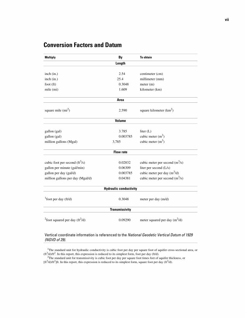
inch (in.) 2.54 centimeter (cm)

inch (in.) 25.4 millimeter (mm)

foot (ft) 0.3048 meter (m)

mile (mi) 1.609 kilometer (km)

Area

square mile (mi2) 2.590 square kilometer (km2)

Volume

gallon (gal) 3.785 liter (L)

gallon (gal) 0.003785 cubic meter (m3)

million gallons (Mgal) 3,785 cubic meter (m3)

Flow rate

cubic foot per second (ft3/s) 0.02832 cubic meter per second (m3/s)

gallon per minute (gal/min) 0.06309 liter per second (L/s)

gallon per day (gal/d) 0.003785 cubic meter per day (m3/d)

million gallons per day (Mgal/d) 0.04381 cubic meter per second (m3/s)

Hydraulic conductivity

1foot per day (ft/d) 0.3048 meter per day (m/d)

Transmissivity

2foot squared per day (ft2/d) 0.09290 meter squared per day (m2/d)

Vertical coordinate information is referenced to the National Geodetic Vertical Datum of 1929 (NGVD of 29).

1The standard unit for hydraulic conductivity is cubic foot per day per square foot of aquifer cross-sectional area, or (ft3/d)/ft2. In this report, this expression is reduced to its simplest form, foot per day (ft/d).

2The standard unit for transmissivity is cubic foot per day per square foot times feet of aquifer thickness, or [ft3/d)/ft2]ft. In this report, this expression is reduced to its simplest form, square foot per day (ft2/d).

Documentation of Revisions to the Regional Aquifer System Analysis Model of the New Jersey Coastal Plain

By Lois M. Voronin

Abstract

The model, which simulates flow in the New Jersey Coastal Plain sediments, developed for the U. S. Geological Survey Regional Aquifer System Analysis (RASA) program was revised. The RASA model was revised with (1) a rediscret­ization of the model parameters with a finer cell size, (2) a spa­tially variable recharge rate that is based on rates determined by recent studies and, (3) ground-water withdrawal data from 1981 to 1998.

The RASA model framework, which subdivided the Coastal Plain sediments into 10 aquifers and 9 confining units, was preserved in the revised model. A transient model that sim­ulates flow conditions from January 1, 1968, to December 31, 1998, was constructed using 21 stress periods.

The model was calibrated by attempting to match the sim­ulated results with (1) estimated base flow for five river basins, (2) measured water levels in long-term hydrographs for 28 selected observation wells, and (3) potentiometric surfaces in the model area for 1978, 1983, 1988, 1993, and 1998 condi­tions. The estimated and simulated base flow in the five river basins compare well. In general, the simulated water levels matched the interpreted potentiometric surfaces and the mea­sured water levels of the hydrographs within 25 feet.

Introduction

As part of an ongoing program to maintain ground-water-flow models constructed in New Jersey, the U.S. Geological Survey (USGS), in cooperation with New Jersey Department of Environmental Protection (NJDEP), developed a standardized procedure to archive the models and revise selected models by incorporating recent data, such as withdrawal data and simula­tion techniques. The Regional Aquifer System Analysis finite-difference numerical model of flow in the New Jersey Coastal Plain sediments (Martin, 1998) was revised by (1) rediscretiz­ing the model parameters with a finer cell size, (2) using a spa­tially variable recharge rate that is based on rates determined in studies conducted since the model was initially developed in

1981 and, (3) using recent ground-water withdrawal data for 1981-98.

The New Jersey Coastal Plain flow model was constructed in 1978 for the U.S Geological Survey Regional Aquifer Sys­tem Analysis (RASA) program (Martin, 1998). The objective of the RASA program was to appraise the major ground-water sys­tems in the United States. For the RASA program in New Jer­sey, a regional model of flow in 10 aquifers and through 9 inter­vening confining units that compose the New Jersey Coastal Plain sediments was developed. Because of the large model area, 9,000 mi2, and the limited computer capabilities, the model was designed with a coarse grid. Cell size ranged from 6.25 mi2 in the southeastern Coastal Plain to 47.5 mi2 in off­shore areas.

The goals of the RASA program were met with the original model design; however, the current water-management needs in New Jersey require a more detailed model that incorporates recent simulation techniques and the most recent (1998) ground-water withdrawal data. Instead of constructing a new model of the New Jersey Coastal Plain sediments, the RASA model was updated.

In 1986 in response to rapidly declining water levels in the New Jersey Coastal Plain, the NJDEP designated Critical Water-Supply Areas 1 and 2 (fig. 1). Critical Area 1 is located in parts of Middlesex, Monmouth, and Ocean Counties. With­drawals from the Wenonah-Mount Laurel aquifer, Englishtown aquifer system, and the Upper and Middle Potomac-Raritan-Magothy aquifers within Critical Area 1 were restricted begin­ning in 1989. Critical Area 2 is located in Camden and parts of Atlantic, Burlington, Cumberland, Gloucester, Monmouth, Ocean, and Salem Counties. Ground-water withdrawals from the Upper, Middle, and Lower Potomac-Raritan-Magothy aqui­fers in Critical Area 2 were restricted beginning in 1996. As a result of the reduced ground-water withdrawals in these areas, water levels have risen as much as 110 ft from 1988 to 1998(Lacombe and Rosman, 2001). The updated RASA model can be used to evaluate the regional effect of reduced ground­water withdrawals on water levels and as a tool to re-evaluate water-management strategies in these areas.

2 Documentation of Revisions to the Regional Aquifer System Analysis Model of the New Jersey Coastal Plain

77 73 7276 75 74

41

40

39

38

37

NEW YORK CONNECTICUT

LONG ISLAND

DE

LAW

AR

E

VIRGINIA

OCEANMODEL BOUNDARYFALL LINE

Coastal Plain

NEW JERSEY

STUDYAR

EAB

OU

ND

AR

Y

0 25 50 MILES

0 25 50 KILOMETERS

75 74

41

40

39

0 20 KILOMETERS

10 20 MILES0

CONNECTI

CUT

NEW YORK

ATLA

NT

IC

OC

EA

N

NEW YORK

SUSSEX

MORRIS

BERGEN

ESSEX

HU

DS

ON

UNION

MIDDLESEX

MONMOUTHMERCER

SOMERSET

HUNTERDON

OCEAN

CAMDENGLOUCESTER

SALEM

CUMBERLAND

CAPE

KENT

NE

WC

AS

TLE

Modified from Martin, 1998

From N.J. Department of Environmental Protection unpublished, 1:250,000. Boundaries are approximate and should not be used for regulatory compliance purposes.

FALL

LINE

PENNSYLVANIA

MARYLAND

ATLANTIC

10

PENNSYLVANIA

DE

LAW

AR

E

WARREN

BURLINGTON

ATLANTIC

MAY

PASSAIC

Water-Supply Critical Area--

EXPLANATION

Critical Area #1

Critical Area #2

Base from U.S. Geological Survey Modified from Watt, 2000digital line graph files, 1:24,000

Figure 1. Location of study area and Critical Water Supply areas 1 and 2 in New Jersey.

3 Introduction

The revised RASA model also can be used to evaluate the regional effect on water levels of a proposed increase in ground­water withdrawals of 2,017 Mgal/d in Salem and Gloucester Counties. This area is adjacent to an area that has experienced water-level declines of more than 100 ft since pumping began in the early 1900’s. Results of the withdrawal scenarios can be used to evaluate alternative resource-management strategies in these areas.

Purpose and Scope

The purpose of this report is to document the revisions made to the RASA model (Martin, 1998). The report includes a detailed analysis of the calibration. Values for simulated and estimated base flow in five river basins in the New Jersey Coastal Plain are presented in tables and hydrographs of simu­lated and measured water levels in 28 observation wells, and simulated and interpreted potentiometric surfaces for 1998 con­ditions are shown in figures. The model simulates withdrawal conditions from 1968 to 1998.

Location and Extent of Study Area

The extent of the model area shown in figure 1 is the same as that of the RASA model. The RASA model includes all of the New Jersey Coastal Plain sediments and extends into New Cas­tle County, Delaware and Philadelphia and Bucks Counties, Pennsylvania. For this study, revisions were made only to an area within the New Jersey Coastal Plain sediments, which is indicated by the shading on the inset map shown in figure 1. The study area is smaller than the model area, includes all of New Jersey, and extends offshore about 20 mi in the southeast.

Previous Investigations

The two previous studies where simulation techniques were used to investigate the regional ground-water flow system of the New Jersey Coastal Plain are listed in table 1 along with the year of the most recent water-level data and the minimum cell size. Studies conducted prior to 1980 were limited in extent and focused on ground-water flow in one aquifer; these studies are not cited in this report. Martin (1998) developed the first regional ground-water-flow model that included all the aquifers of the New Jersey Coastal Plain (RASA model). Pope and Gor­don (1999) expanded on Martin’s work and simulated ground­

water flow in the New Jersey Coastal Plain aquifers that extend to the Continental Shelf (CP model).

Conceptual Hydrogeologic Model

The hydrogeology of the New Jersey Coastal Plain is dis­cussed briefly in this section. The New Jersey Coastal Plain sed­iments are described in detail by Zapecza (1989).

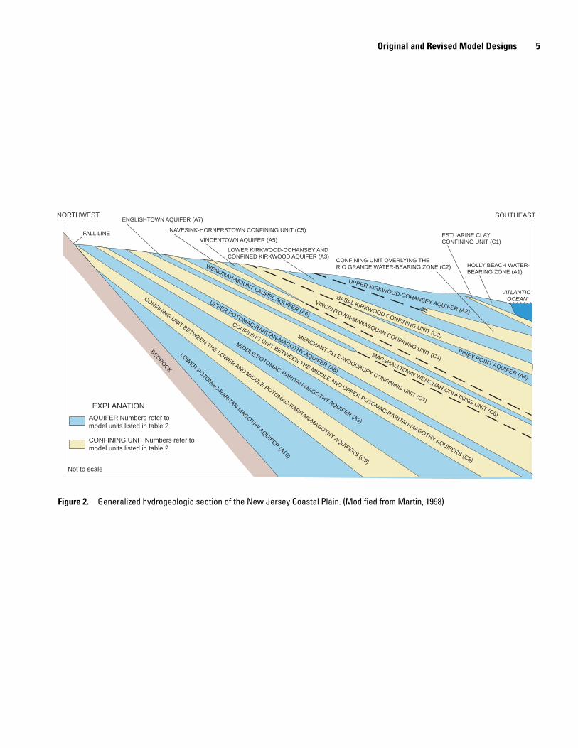
Hydrogeologic Framework

The New Jersey Coastal Plain sediments consist of alter­nating layers of gravel, sand, silt, and clay that gently dip and thicken to the southeast and overlie crystalline bedrock (fig. 2). Most aquifers and confining units in the New Jersey Coastal Plain were mapped by Zapecza (1989). Martin (1998) modified the hydrogeologic framework presented in the report by Zapecza for the RASA model and represented the Coastal Plain sediments as 10 major aquifers and 9 intervening confining units.

Ground-Water-Flow System

The Coastal Plain ground-water-flow system is dynamic (changes with time) and has changed greatly in response to ground-water withdrawals. A brief discussion of the current (1998) ground-water-flow system is given here. For a more detailed discussion of the ground-water-flow system see Martin (1998). Ground-water flow in the New Jersey Coastal Plain sed­iments under current conditions (1998) is affected by the hydraulic properties of the saturated sediments, topography, and ground-water withdrawals. In general, topographic highs are recharge areas and topographic lows are discharge areas. Ground-water withdrawals in topographic lows can reverse ground-water-flow directions in these areas, which then can become ground-water recharge areas. Discharge areas in the New Jersey Coastal Plain include the Atlantic Ocean, the Dela­ware River, the Delaware and Raritan Bays, and streams. Exam­ples of recharge areas are the high-altitude areas (250 ft., NGVD of 1929) in northwestern Monmouth County.

In general, aquifers transmit water easily compared to con­fining units, which transmit water only to a small extent. Flow within confining units is predominantly vertical as a result of large vertical gradients within confining units. Flow within aquifers is horizontal with a small vertical component.

Table 1. Previous simulation studies conducted for the New Jersey Coastal Plain

[RASA, Regional Aquifer System Analysis; CP, Coastal Plain]

Model (acronym) Reference Most recent water-level data used in

study

Minimum cell size (square miles)

RASA Martin (1998) 1978 6.25 CPOP Pope and Gordon (1999) 1988 6.25

4 Documentation of Revisions to the Regional Aquifer System Analysis Model of the New Jersey Coastal Plain

Six steep regional cones of depression have developed in the New Jersey Coastal Plain. Two cones are centered in south­ern Monmouth and northwestern Ocean Counties, three in cen­tral Camden County, and one in southeastern Atlantic County (Lacombe and Rosman, 2001, sheets 3, 6, 7, 8, 9, 10). All of these regional cones of depression have developed in response to the decline in water levels that resulted from large ground­water withdrawals that began in the late 1800’s.

Original and Revised Model Designs

The RASA model was compiled on an early computer sys­tem for a multi-layer finite-difference ground-water-flow model. The model computer code used to simulate ground­water flow was a modified version (Leahy, 1982) of the com­puter program developed by Trescott (1975). For this study, the input data were formatted for use with MODFLOW-96, a ver­sion of the modular finite-difference ground-water-flow model by Harbaugh and McDonald (1996).

Model Approach

For the quasi-three dimensional representation of the aqui­fers and confining units of the New Jersey Coastal Plain, flow is assumed to be entirely horizontal within the aquifers and ver­tical through the confining units. Water levels within the con­fining units were not simulated, but vertical flow through the confining units was calculated by using vertical leakance (ver­tical hydraulic conductivity divided by thickness). The RASA model assignment of the Coastal Plain sediments into aquifers and confining units was not changed in the revised model. The geologic and hydrogeologic units and the corresponding model-layer designations used in the model are listed in table 2. A gen­eralized hydrogeologic section of the New Jersey Coastal Plain and the designated model layers are shown in figure 2. A sche­matic representation of the model units used to represent the hydrogeologic units (fig. 2) is shown in figure 3. Martin (1998) modeled the 10 major aquifers and the streams using an 11­layer model. Martin modeled the streams as a layer. In the revised model, the streams were modeled using the river and drain package of MODFLOW-96. Hence, an 11th layer was not needed in the revised model.

Grid Design

The RASA grid cell size was 6.25 mi2 in the northern and southwestern New Jersey Coastal Plain, 9.375 mi2 in the south­eastern Coastal Plain, and as much as 47.5 mi2 in offshore areas (plate 1). The grid had 29 rows and 51 columns. In the new grid (plate 1) with 135 rows and 245 columns, the cell size is 0.25 mi2 in the northern and southwestern New Jersey Coastal Plain, 0.31 mi2 in the southeastern Coastal Plain, and as much as 3.16

mi2 in offshore areas. The ratio of the number of new cells to the original number of cells is 25 to 1 in onshore areas.

Rows 1 and 29 and columns 1 and 51 were not active in the RASA model and are not included as part of the grid area of the revised model. The relation between the RASA and revised model grids is shown in plate 1.

Ground-Water Withdrawals

A transient ground-water-flow model that simulates condi­tions from January 2, 1968, to December 31, 1998, was con­structed with 21 stress periods and 10 time steps within each stress period. Ground-water withdrawal data used in the revised model are those reported to the NJDEP by water purveyors. The withdrawal data also are maintained in a USGS computer data­base. Average annual withdrawals were used for all stress peri­ods (fig. 4). Because stress periods 4 through 21 are 1 year in length, average annual withdrawals are equivalent to total annual withdrawals during these stress periods. Withdrawals for stress periods 1 to 3 are the same as withdrawals for stress periods 7, 8, and 9 of the RASA model. Stress period 1 extended from January 2, 1968, to January 1, 1973; period 2, January 2, 1973, to January 1, 1978; and period 3, January 2, 1978, to Jan­uary 1, 1981, in the RASA model. Annual ground-water with­drawals for these three stress periods were averaged for these 3- to 5-year time periods. In the revised model, stress periods 2 and 3 have the same time periods as stress periods 8 and 9 in the RASA model; however, stress period 1 in the revised model represents an interval of 100 years.

The use of a time interval of 100 years enabled the model to simulate steady-state flow conditions using average ground­water withdrawals from January 2, 1968, to January 1, 1973. Initial water levels for this period were the water levels calcu­lated from the original model for average conditions during 1968-73. During the sensitivity analysis of the effects of with­drawals on the ground-water-flow system, Martin (1998) found that after 10 years with a constant pumping rate the change in water levels would be less than 1 ft/yr anywhere in the aquifer system. A period of 100 years was more than enough time to simulate steady-state flow conditions with average from Janu­ary 2, 1968, to January 1, 1973, ground-water withdrawals. In Martin (1998), water-level changes simulated after only 10 years also were slight, such that the residual effect of changes in withdrawals rates prior to 1968 (if they were simulated) would have little effect on the simulated response during the period of interest, after 1978.

Water levels simulated with the revised model at the end of stress periods 1, 2, and 3 are comparable to those at the end of stress period 7, 8, and 9 simulated with the RASA model. Water levels at the end of stress period 2 are comparable to the 1978 water levels that Martin (1998) used for calibration.

model units listed in table 2

model units listed in table 2

Not to scale

LOWER POTOMAC-RARITAN-MAGOTHY

AQUIFER (A10)

MIDDLE POTOMAC-RARITAN-MAGOTHY AQUIFER (A9)

UPPER POTOMAC-RARITAN-MAGOTHY AQUIFER (A8)

CONFINING UNIT BETWEENTHE LOWER AND MIDDLE POTOMAC-RARITAN-MAGOTHY AQUIFERS (C9)

CONFINING UNIT BETWEEN THE MIDDLE AND UPPER POTOMAC-RARITAN-MAGOTHY AQUIFERS (C8)

MERCHANTVILLE-WOODBURY CONFINING UNIT (C7)

BEARING ZONE (A1)

BASAL KIRKWOOD CONFINING UNIT (C3)

PINEY POINT AQUIFER (A4)

VINCENTOWN-MANASQUAN CONFINING UNIT (C4)

WENONAH-MOUNT LAUREL AQUIFER (A6)

UPPER KIRKWOOD-COHANSEY AQUIFER (A2)

SOUTHEAS TN

OCEAN

BEDROCK

MARSHALLTOWN WENONAH CONFINING UNIT (C6)

5

Figure 2.

AQUIFER Numbers refer to

CONFINING UNIT Numbers refer to

EXPLANA TION

ENGLISHT OWN AQUIFER (A7)

F ALL LINE

HOLL Y BEACH W A TER-

ESTUARINE CLA Y CONFINING UNIT (C1)

CONFINING UNIT OVERL YING THE RIO GRANDE W A TER-BEARING ZONE (C2)

VINCENT OWN AQUIFER (A5)

NA VESINK-HORNERST OWN CONFINING UNIT (C5)

OR THWEST

ATLANTIC

LOWER KIRKWOOD-COHANSEY AND CONFINED KIRKWOOD AQUIFER (A3)

Original and Revised Model Designs

Generalized hydrogeologic section of the New Jersey Coastal Plain. (Modified from Martin, 1998)

6 Documentation of Revisions to the Regional Aquifer System Analysis Model of the New Jersey Coastal Plain

DOWNDIP

S A2

C2 A3

C3

A1

C1

S

Atlantic OceanS

A4

C4

S

A5

C5 P5

S

A6

C6

S

P6

S

S

P7

S

A7

C7

S

A8

C8

S

S A9

C9 A10

UPDIP

FALL LINE

EXPLANATION

A1

C1

AQUIFER-Number refers to model unit RECHARGE TO OUTCROP AREA OF AQUIFER-listed in table 2 Recharge rate greater than 1 inch per year

CONFINING UNIT-Numbers refers to model unit RECHARGE TO OUTCROP AREA OF CONFING listed in table 2 UNIT-Recharge rate less than 1 inch per year

S SURFACE-WATER STAGE NO-FLOW BOUNDARY

STREAMBED OR LAKEBED CONDUCTANCE FLUX BOUNDARYIN OUTCROP AREA

VERTICAL HYDRAULIC CONNECTION BETWEEN OUTCROP AREA OF CONFINING UNIT SIMULATED AS CONFINING UNITS--Aquifer is absent

P5 AN AQUIFER LAYER-Number refers to model layer representingthe vertical flux through the confing-unit outcrop area

Figure 3. Schematic representation of aquifers, confining units, and boundary conditions used in the revised New Jersey Coastal Plain ground-water-flow model. (Modified from Martin, 1998, figure 4)

Table 2. Geologic and hydrogeologic units of the New Jersey Coastal Plain and model units in the revised Regional Aquifer SystemAnalysis model

7 Original and Revised Model Designs

Table 2. Geologic and hydrogeologic units of the New Jersey Coastal Plain and model units in the revised Regional Aquifer System Analysis model [Modified from Zapecza (1989, table 2) and Seaber (1965, table 3); shading indicates adjacent geologic or hydrogeologic unit is not defined; letter and number in parentheses is the model layer]

SYSTEM SERIES GEOLOGIC UNIT HYDROGEOLOGIC UNIT

Updip

MODEL UNITS3

Downdip

Alluvial

Quaternary

Holocene deposits

Beach sand and gravel

Undifferentiated Upper Kirkwood-Cohansey aquifer (A2) Holly Beach water-bearing zone (A1)

Pleistocene Cape May Formation

Kirkwood­Cohansey1

Estuarine Clay confining unit (C1)

Upper Kirkwood-Cohansey aquifer (A2)

Pennsauken Formation

Bridgeton Formation

Beacon Hill Gravel

Cohansey Sand Kirkwood-Cohansey

aquifer system Lower Kirkwood-Cohansey aquifer (A3)

Miocene

Pot

omac

-Rar

itan

-M

agot

hy

Com

posi

te c

onfi

ning

uni

t aq

uife

r sy

stem

Confining unit overlying the Rio Grande Confining unit water-bearing zone (C2) Kirkwood Formation

Rio Grande2Tertiary

Confining unit Confined Kirkwood aquifer (A3) Atlantic City 800-foot sand

Basal Kirkwood confining unit (C3)

Oligocene Piney Point Piney Point Piney Point aquifer (A4) Formation aquifer

Shark RiverFormationEocene Vincentown-Manasquan confining unit (C4)

Manasquan Formation

Vincentown Vincentown Formation Vincentown aquifer (A5) aquifer PaleoceneHornerstown Sand

Tinton Sand

Red Bank Navesink-Hornerstown confining unit (C5) Red Bank Sand sand

Navesink Formation

Mount Laurel Sand Wenonah-Mount Laurel aquifer Wenonah-Mount Laurel aquifer (A6)

Wenonah FormationMarshalltown-Wenonah Marshalltown-Wenonah confining unit (C6)

Marshalltown Formation confining unit

Englishtown aquifer Englishtown Formation Englishtown aquifer (A7) system Cretaceous

Cretaceous

Upper

Woodbury Clay Merchantville-Woodbury confining unit Merchantville-Woodbury confining unit (C7) Merchantville Formation

UpperMagothy Formation Upper Potomac-Raritan-Magothy aquifer (A8) aquifer

Confining Confining unit between the Middle and Upper Potomac-Raritan-Magothy aquifers (C8) unitRaritan Formation

Middle Middle Potomac-Raritan-Magothy aquifer (A9) aquifer

Confining Confining unit between the Lower and Middle Potomac-Raritan-Magothy aquifers (C9) unitPotomac Group

Lower Lower Lower Potomac-Raritan-Magothy aquifer (A10) Cretaceous aquifer

Pre-Cretaceous Bedrock Bedrock confining unit 1Kirkwood-Cohansey aquifer system. 2Rio Grande water-bearing zone. 3‘A’ refers to modeled aquifer. ‘C’ refers to modeled confining unit, number refers to model unit.

8 Documentation of Revisions to the Regional Aquifer System Analysis Model of the New Jersey Coastal Plain

400

350

300

250

1968 1970 1972 1974 1976 1978 1980 1982 1984 1986 1988 1990 1992 1994 1996 1998 2000

for each stress period for each stress period

Stress period

1

2 3 4 5

6 7

8 9

10

11 12

13 14

15 16

17 18

19 20

21

Average withdrawals Total annual withdrawals

YEAR

Figure 4. Average and total annual ground-water withdrawals for each stress period for the New Jersey Coastal Plain, 1968-98.

WIT

HD

RA

WA

LS, I

N M

ILLI

ON

GA

LLO

NS

PE

R D

AY

9

Lateral and Lower Boundary Conditions

The model boundaries in the revised model are the same as those used in the 11-layer RASA model (plate 1). The model boundaries are shown in a cross section view in figure 3. A sum­mary of the boundary conditions is given here. For a detailed discussion of the model boundaries and the different boundaries used for the 11-layer RASA model, refer to Martin (1998).

The generalized lateral boundaries shown in plate 1 are not the same in every aquifer simulated in the model, but vary slightly among aquifers. The northwestern updip limit of all model layers is the limit of the Coastal Plain sediments, which is located at or within 15 mi of the Fall Line. The updip limit of the aquifers is modeled as a no-flow boundary.

The Coastal Plain sediments overlie crystalline bedrock, and the lower boundary of the model is at this contact. It is likely that no flow occurs between the Coastal Plain sediments and the crystalline bedrock. This boundary also is modeled as a no-flow boundary.

The lateral model boundaries in the northeast and south­west are specified-flux boundaries that originally were derived from a model of the North Atlantic Coastal Plain (Leahy and Martin, 1993) for the RASA model. For the model by Leahy and Martin, the model area extends from Long Island, New York, to North Carolina and includes all of the New Jersey Coastal Plain. The northeast and southwest boundaries roughly approximate a flow line, and specified fluxes were applied only in areas where the aquifer intersects the flow boundary.

Flows at the lateral boundaries in the northeast and south­west for stress periods 1 to 3 are those used in the original RASA model. Flows at the lateral boundaries for stress periods 4 to 21 for all aquifers, except the Potomac-Raritan-Magothy aquifer system for stress periods 19 to 21, were calculated by using the New Jersey Coastal Plain model constructed by Pope and Gordon (1999). Flows at the lateral boundaries in the Poto-mac-Raritan-Magothy aquifer system for stress periods 19 to 21 also were calculated by using the model by Pope and Gordon (1999), except those at the Delaware and New Jersey boundary. Outward lateral fluxes were increased in those stress periods to reflect the large increase in ground-water withdrawals in Dela­ware. The increase in boundary flows was necessary to ensure that simulated water levels would match the water levels in the cone of depression that has developed in the Potomac-Raritan-Magothy aquifer system at the Delaware and New Jersey State line since 1988. The lateral boundary flow for each stress period and the ground-water withdrawals for each aquifer are listed in table 3.

The southeastern downdip boundary in the Potomac-Rari-tan-Magothy aquifer system is a stationary no-flow boundary and is located at the downdip limit of freshwater in the aquifer. The downdip limit of freshwater was determined by Meisler (1980) and is shown on the potentiometic-surface maps pre­sented later in this report.

The southeastern boundary in the confined Kirkwood aquifer and the upper Kirkwood-Cohansey aquifer is also a specified-flux boundary. The lateral boundary flows for stress

Original and Revised Model Designs

periods 1 to 3 are those used in the RASA model. The lateral boundary flows for stress periods 4 to 21 were calculated by using the New Jersey Coastal Plain model constructed by Pope and Gordon (1999).

The Englishtown aquifer system and the Wenonah-Mount Laurel, Vincentown, and Piney Point aquifers (table 2) are not continuous throughout the New Jersey Coastal Plain. The limit of these aquifers in the southeast is modeled as a no-flow boundary.

Upper Boundary Conditions

The upper boundary of the model is a head-dependent-flux boundary in cells that represent the stream reaches in the model area. The stream stage was estimated from 1:24,000 USGS topographic maps of the model area. The streambed conduc­tance was estimated as the product of the streambed hydraulic conductivity, length of stream reach, and stream width divided by the streambed thickness. The streambed conductance is an aggregate parameter that represents all of the factors that affect flow between the aquifer and the stream.

In onshore areas, the upper boundary is a recharge bound­ary where all applied ground-water recharge flows downward through confining units and aquifers or laterally into aquifers. In offshore areas, the upper boundary is a constant freshwater equivalent water level. The recharge rate and stream stage were kept constant for all stress periods of the transient model. The recharge rate and stream stage are represented by long-term averages and do not reflect seasonal variations. The simulation of yearly hydrologic conditions with long-term averages for recharge and stream stage is consistent with the conceptual model that represents each stress period with average yearly hydrologic conditions.

Streams

A fine grid-cell size allows for a better representation of the streams in the model area. Because of the original large cell size in the RASA model, each cell represented at least one reach of a stream, and in many cells, various reaches of a stream were represented. Consequently, the stream stage for each original cell represented an average stage for a large reach of a stream or various stream reaches. The average stream stage in the new grid is for a stream reach with a maximum length of 4,226 ft, in contrast to 23,796 ft in the RASA grid. Model cells that repre­sent the streams in the study area are shown in figure 5. Cells in the new grid that represent streams were identified by using geographic information system (GIS) coverages of the model grid (generated for this study) and streams (digitized from USGS 1:24,000 topographic maps).

The drain and river packages of MODFLOW-96 were used to simulate the streams in the model area. The river pack­age was used to simulate losing and gaining areas of the Dela­ware River and Raritan Bay. Continually gaining streams, located in other areas, were simulated with the drain package.

Table 3. Average daily ground-water withdrawals from each aquifer and lateral boundary flows by stress period, New Jersey Coastal Plain, 1968-98-9810

Table 3. Average daily ground-water withdrawals from each aquifer and lateral boundary flows by stress period, New Jersey Coastal Plain, 1968-98 [All values are in million gallons per day. Positive boundary flows are out of model area, negative boundary flows are into model area.]

Stress period

Model layer number

1 1/1968 -1/1973

2 1/1973 -1/1978

3 1/1978 -1/1981

4

1981

5

1982

6

1983

7

1984

8

1985

9

1986

10

1987

11

1988

12

1989

A1 0.08 0.11 0.17 0.24 0.25 0.25 0.16 0.01 0.01 0.01 0.01 0.01

A2 38.93 43.87 48.57 60.06 57.85 61.77 64.07 74.55 80.69 77.38 74.35 71.26

A3 30.42 36.95 38.02 23.08 23.30 23.44 23.29 23.96 26.50 25.58 24.16 25.35

A4 1.48 1.97 2.00 1.81 2.02 1.97 1.79 1.77 2.12 2.01 2.11 1.84

A5 0.09 0.94 1.15 1.47 1.02 1.14 1.00 0.99 1.23 1.36 1.94 1.50

A6 4.65 4.56 4.97 4.65 4.66 6.05 6.07 6.28 6.84 6.50 7.65 7.78

A7 11.33 11.95 11.27 11.17 10.52 10.10 9.99 10.51 10.59 10.72 10.48 10.04

A8 85.93 84.79 85.44 81.99 85.91 87.39 81.24 81.58 83.15 81.52 75.87 74.92

A9 80.92 91.81 91.79 81.59 80.14 81.68 73.21 74.67 79.54 79.38 82.21 75.92

A10 71.83 73.95 74.82 76.41 74.34 79.67 74.17 75.20 69.34 67.25 73.59 66.11

Total 325.66 350.9 358.2 342.47 340.01 353.46 334.99 349.52 360.01 351.71 352.37 334.73 Net boundary flow -3.2 -5.2 -5.6 1.1 1.1 1.1 1.1 1.1 1.1 1.1 1.1 1.1

Model layer

A1 - Holly Beach water-bearing zone

A2 - Upper Kirkwood-Cohansey aquifer

A3 - Lower Kirkwood-Cohansey and confined Kirkwood aquifers

A4 - Piney Point aquifer

A5 - Vincentown aquifer

A6 - Wenonah-Mount Laurel aquifer

A7 - Englishtown aquifer system

A8 - Upper Potomac-Raritan-Magothy aquifer

A9 - Middle Potomac-Raritan-Magothy aquifer

A10 - Lower Potomac-Raritan-Magothy aquifer

Docum

entation of Revisions to the Regional Aquifer System

Analysis M

odel of the New

Jersey Coastal Plain

Table 3. Average daily ground-water withdrawals from each aquifer and lateral boundary flows by stress period, New Jersey Coastal Plain, 1968-98---Continued11

Table 3. Average daily ground-water withdrawals from each aquifer and lateral boundary flows by stress period, New Jersey Coastal Plain, 1968-98—Continued

Stress period

Model layer number

13 1990

14 1991

15 1992

16 1993

17 1994

18 1995

19 1996

20 1997

21 1998

A1 0.01 0.09 0.01 0.09 0.08 0.07 0.03 0.16 0.17

A2 83.00 95.63 95.30 83.43 93.73 100.70 83.53 112.10 105.14

A3 22.66 22.80 20.90 21.93 23.99 23.07 21.37 24.15 24.40

A4 1.87 2.23 2.29 3.32 3.25 2.89 3.60 3.81 4.50

A5 1.24 1.73 1.62 1.77 1.46 1.33 1.36 1.46 1.50

A6 6.56 6.16 6.33 6.78 6.39 7.72 6.31 10.19 9.15

A7 9.19 7.20 6.98 6.94 6.95 7.43 6.49 8.94 7.78

A8 73.94 72.22 69.38 68.28 66.38 66.19 59.04 62.64 67.26

A9 72.60 68.14 66.40 64.74 63.82 63.64 57.98 59.94 62.24

A10 62.77 58.83 58.53 52.23 57.08 59.23 47.45 44.61 47.96

Total 333.84 335.03 327.74 309.51 323.13 332.27 287.16 328.00 330.10 Net boundary

flow 0.4 0.4 0.4 0.4 0.4 0.4 0.9 0.9 0.9

Model layer

A1 - Holly Beach water-bearing zone

A2 - Upper Kirkwood-Cohansey aquifer

A3 - Lower Kirkwood-Cohansey and confined Kirkwood aquifers

A4 - Piney Point aquifer

A5 - Vincentown aquifer

A6 - Wenonah-Mount Laurel aquifer

A7 - Englishtown aquifer system A8 - Upper Potomac-Raritan-Magothy aquifer A9 - Middle Potomac-Raritan-Magothy aquifer A10 - Lower Potomac-Raritan-Magothy aquifer

Original and Revised M

odel Designs

05

1015

MIL

ES

05

1015

KIL

OM

ET

ER

S

PE

NN

SY

LVA

NIA

ME

RC

ER

MID

DLE

SE

X

MO

NM

OU

TH

CA

MD

EN

GLO

UC

ES

TE

RS

ALE

M

AT

LAN

TIC

CA

PE

MA

Y

NE

W Y

OR

K

AT

LA

NT

IC

O

CE

AN

DE

LAW

AR

EB

AY

RA

RIT

AN

BAY

Bas

e fr

om U

.S. D

epar

tmen

t of A

gric

ultu

reS

oil C

onse

rvat

ion

Ser

vice

, 1:2

50,0

00, 1

980

Coh

anse

y River

Del

awar

eR

iver

Rari ta

nR

iver

Naves

ink

Riv

erM

anasquan River

To

ms River

Batst

oRive

r

Mullica River

Mau

rice

River

GreatEggHarbourRiver

BU

RLI

NG

TO

N

OC

EA

N

Loca

tion

of s

trea

m r

each

in th

e ou

tcro

p ar

ea o

f mod

el la

yer A

1

Loca

tion

of s

trea

m r

each

in th

e ou

tcro

p ar

ea o

f mod

el la

yer A

2

Loca

tion

of s

trea

m r

each

in th

e ou

tcro

p ar

ea o

f mod

el la

yer A

3

Loca

tion

of s

trea

m r

each

in th

e ou

tcro

p ar

ea o

f mod

el la

yer A

5an

d th

e co

mpo

site

con

finin

g un

its s

imul

ated

as

part

of m

odel

laye

r A5

Loca

tion

of s

trea

m r

each

in th

e ou

tcro

p ar

ea o

f mod

el la

yer A

6an

d th

e M

arsh

allto

wn-

Wen

onah

con

finin

g un

it si

mul

ated

as

part

of m

odel

laye

r A6

EX

PLA

NA

TIO

N

MARYLAND

DELAWARE

75

39

40

75

74

74

39

Bar

nega

t Lig

ht

Loca

tion

of s

trea

m r

each

in th

e ou

tcro

p ar

ea o

f mod

el la

yer A

7an

d th

e M

erch

antv

ille-

Woo

dbur

y co

nfin

ing

unit

sim

ulat

ed a

s pa

rt o

f mod

el la

yer A

7

Loca

tion

of s

trea

m r

each

in th

e ou

tcro

p ar

ea o

f mod

el la

yer A

8

Loca

tion

of s

trea

m r

each

in th

e ou

tcro

p ar

ea o

f mod

el la

yer A

9

Loca

tion

of s

trea

m r

each

in th

e ou

tcro

p ar

ea o

f mod

el la

yer A

10

CU

MB

ER

LAN

D

12 Documentation of Revisions to the Regional Aquifer System Analysis Model of the New Jersey Coastal Plain

Figu

re 5

. M

odel

cel

ls th

at re

pres

ent s

tream

reac

hes

in th

e st

udy

area

, New

Jer

sey

Coas

tal P

lain

.

Recharge

The upper model boundary includes a spatially variable recharge rate applied at cells that represent the outcrop area of aquifers and confining units without wetlands. The recharge rate applied to the outcrop areas represents long-term precipita­tion minus long-term evapotranspiration and surface-water run­off. The amount of precipitation that results in surface-water runoff is related to the topography and lithology of the outcrop areas. The spatially variable recharge rate reflects these changes in the outcrop areas of eight aquifers and three confining units in the Coastal Plain. The Piney Point aquifer, the Lower Poto-mac-Raritan-Magothy aquifer, the Estuarine Clay confining unit, and the confining unit overlying the Rio Grande water-bearing zone (table 2) do not crop out in the model area and receive no recharge at the upper model boundary. The confining unit between the Middle and Upper Potomac-Raritan-Magothy aquifers and the confining unit between the Lower and Middle Potomac-Raritan-Magothy aquifers either crop out under the Delaware River or are simulated as receiving no recharge at the upper model boundary because the width of the outcrop area is negligible, less than 0.5 mi. Zapecza (1989) does not map an outcrop area for these confining units. Barton and Kozinski (1991) and Lewis and others (1991) show these units to have limited outcrop areas, less than 0.5 mile wide in their respective study areas.

The precipitation that recharges the outcrop areas eventu­ally flows to surface-water bodies, such as streams or the ocean, and is referred to as ground-water discharge. Ground-water dis­charge can be local flow to nearby streams within the shallow aquifer system, intermediate flow along long flow paths (miles) beneath nearby streams that discharge to neighboring larger streams, or regional flow that moves through confining units to confined aquifers and eventually discharges to large rivers and (or) the ocean.

Model Calibration

The revised model was calibrated by trail-and-error adjust­ment of the vertical-leakance values, storage-coefficient values, streambed-conductance values, lateral-boundary fluxes, and recharge rates. Recharge rates were adjusted in areas where no previous studies were conducted that determined a recharge rate. During model calibration, it was found that changes to only the five model parameters listed above improved the RASA model calibration in any particular area; therefore, these param­eters were changed from the RASA model-input data. These five parameters were adjusted during model calibration in order to minimize the difference between simulated and measured values of one or more of the following: (1) estimated base flow for five river basins, (2) water levels in 28 selected observation wells for which long-term hydrographs were available, and (3) potentiometric surfaces for 1978, 1983, 1988, 1993, and 1998 conditions.

Model Calibration 13

Simulated 1978 potentiometric surfaces from the RASA and revised model also were compared during model calibra­tion. The objective of comparing the simulated potentiometric surfaces from the RASA model and revised model was to ensure that the original level of calibration was maintained or improved.

Revisions to Model Input Data

In the following four sections, the revisions to the model-input data for the revised model are described.

Recharge

The recharge rates are based on values determined by stud­ies conducted in the New Jersey Coastal Plain and by model cal­ibration. The recharge rates are shown in figure 6, and the loca­tions of the study areas are shown in figure 7. The recharge rates range from 0.01 in/yr in the outcrop area of the composite con­fining unit to 20 in/yr in the Cohansey aquifer. The recharge rates used in this model are long-term averages and regional estimates. These rates do not reflect seasonal or local variations, which do occur.

Recharge was applied to the modeled outcrop area of three confining units because, on the basis of simulation results, a small amount of recharge could be percolating through the con­fining units to the underlying aquifers. Recharge to confining-unit outcrops could not be simulated directly because confining units are not represented with a layer of cells in the model, but only with vertical-leakance characteristics. Therefore, recharge to confining-unit outcrops is applied to cells with zero transmis­sivity in the layer that represents the overlying aquifer. The out­crop areas of confining units C5, C6, and C7 are labeled p5, p6, and p7, respectively, in figure 3 and are simulated as part of the aquifer overlying the confining unit. For example, the confining unit outcrop area labeled p5 is simulated as part of the aquifer labeled a5. In these areas (p5, p6, and p7 in figure 3), no hori­zontal flow to the aquifer results, only vertical flow through the outcrop area of the confining unit to the underlying aquifer.

Vertical Leakance

The vertical leakance was adjusted for the Navesink-Hor-nerstown confining unit (fig. 8). The vertical-leakance values were decreased a maximum of three orders of magnitude in the vicinity of the wells shown in figure 8, which are screened in the Vincentown and Wenonah-Mount Laurel aquifers, to obtain a better match between the simulated and long-term measured water levels in these wells. Simulated water levels for well 29­139, which is screened in the Vincentown aquifer, are 6 ft closer to measured water levels in 1978 than in the original RASA model. Simulated water levels in well 25-486, which is screened in the Wenonah-Mount Laurel aquifer, are 15 ft closer to measured water levels in 1985 than in the original RASA model. All other vertical-leakance values used in the revised

05

1015

MIL

ES

05

1015

KIL

OM

ET

ER

S

0140

8500

0146

5850

0146

7000

0147

7120

0148

2500

PE

NN

SY

LVA

NIA

NE

W Y

OR

K

AT

LA

NT

IC

O

CE

AN

DE

LAW

AR

EB

AY

RA

RIT

AN

BAY

Bas

e fr

om U

.S. D

epar

tmen

t of A

gric

ultu

reS

oil C

onse

rvat

ion

Ser

vice

, 1:2

50,0

00, 1

980

Coh

anse

y River

Del

awar

eR

iver

Rari ta

nR

iver

Naves

ink

Riv

erM

anasquan River

To

ms River

Batst

oRive

r

Mullica River

Mau

rice

River

GreatEggHarbourRiver

Rec

harg

e ra

te, i

n in

ches

per

yea

r

EX

PLA

NA

TIO

N

MARYLAND

DELAWARE

75

39

40

75

74

74

39

Bar

nega

t Lig

ht

Poi

nt P

leas

ant

Bou

ndar

y of

dra

inag

e ba

sin

drai

ning

to s

trea

mflo

w-g

agin

g st

atio

n

Str

eam

flow

-gag

ing

stat

ion

and

num

ber

0148

2500

0.01

0.8

6 9

15 16 17 20

14 Documentation of Revisions to the Regional Aquifer System Analysis Model of the New Jersey Coastal Plain

Figu

re 6

. Re

char

ge ra

tes

used

in th

e m

odel

and

the

loca

tion

of s

elec

ted

drai

nage

bas

ins

and

stre

amflo

w-g

agin

g st

atio

ns in

the

mod

el a

rea,

New

Jer

sey

Coas

tal P

lain

.

15 Model Calibration

75

41

40

39

74

0

0

10

10

SALEM

CUMBERLAND

GLOUCESTER CAMDEN

CAPE

OCEAN

MONMOUTH

MIDDLESEXMERCER

SOMERSET

NEW JERSEY

HU

DS

ON

HUNTERDON

SUSSEX

MORRIS

BERGEN

ESSEX

UNION

D E LAW ARE R

IVE

R

FALLLIN

E

Hydrology of the unconfined aquifer system,

5 sheets.

Hydrogeology of the unconfined aquifer

Resources Investigations Report 94-4234, 6 sheets

unconfined aquifer system of the Great Egg Harbor River basin,

Investigations Report 91-4126, 5 pls.

Charles, E.G., Storck, D.A., and Clawges, R.M., 2001, Hydrogeology of the unconfined aquifer system, Maurice River

Johnson, M.L., and Charles, E.G., 1997, Hydrogeology of the unconfined aquifer system, Salem River area: Salem River and Racoon, OJResources Investigations Report 96-5195, 5 sheets

Hydrology of the unconfined aquifer system in the upper Maurice River basin

20 MILES

20 KILOMETERS

ATLANTIC

BURLINGTON

MAY

PASSAIC

WARREN

Watt, M.K., Johnson, M.L. and Lacombe, P.J., 1994

Toms River, Metedeconk River, and Kettle Creek Basins, New Jersey, 1987-90: U.S. Geological Survey Water-Resources Investigations Report 93-4110,

Johnson, M.L., and Watt, M.K., 1996,

system, Mullica River Basin, New Jersey, 1991-92: U.S. Geological Survey Water-

Watt, M.K. and Johnson, M.L., 1992, Water resources of the

New Jersey, 1989-90: U.S. Geological Survey Water-Resources

ldmans, Alloway, and Stow Creek Basins, New ersey, 1993-94: U.S. Geological Survey Water-

Lacombe, P.J. and Rosman, R., 1995,

and adjacent areas in Gloucester County, New Jersey, 1986-87: U.S. Geological Survey Water-Resources Investigations Report 92-4128,

Watt, M.K., Kane, A.C., Charles, E.G., and Storck, D.A., 2003, Hydrology of the unconfined aquifer system, Rancocas Creek area: Rancocas, Crosswicks, Assunpink, Blacks, and Crafts Creek Basins, New Jersey, 1996: U.S. Gelogical Survey Water-Resources Investigations Report 02-4280, 5 sheets5 sheets

Spitz, F.J., 1998, Analysis of ground-water flow and saltwater area: Maurice and Cohansey River basins, New Jersey, 1994-95: encroachment in the shallow aquifer system of Cape May County, U.S. Geological Survey Water-Resources Investigations Report New Jersey: U.S. Geological Survey Water-Supply Paper 2490, 01-4229, 5 sheets 51 p.

Figure 7. Location of, and references for, studies that reported ground-water recharge rates in the New Jersey Coastal Plain.

29-1

3825

-637

25-4

29

25-4

86

25-3

53

05

1015

MIL

ES

05

1015

KIL

OM

ET

ER

S

PE

NN

SY

LVA

NIA

ME

RC

ER

MID

DLE

SE

X

MO

NM

OU

TH

CA

MD

EN

GLO

UC

ES

TE

RS

ALE

M

AT

LAN

TIC

CA

PE

MA

Y

NE

W Y

OR

K

AT

LA

NT

IC

O

CE

AN

DE

LAW

AR

EB

AY

RA

RIT

AN

BAY

Bas

e fr

om U

.S. D

epar

tmen

t of A

gric

ultu

reS

oil C

onse

rvat

ion

Ser

vice

, 1:2

50,0

00, 1

980

Coh

anse

y River

Del

awar

eR

iver

Rari ta

nR

iver

Naves

ink

Riv

erM

anasquan River

To

ms River

Batst

oRive

r

Mullica River

Mau

rice

River

GreatEggHarbourRiver

BU

RLI

NG

TO

N

OC

EA

N

1 x

10E

t

o 5

x 10

E

5 x

10E

t

o 5

x 10

E

5 x

10E

t

o 5

x 10

E

EX

PLA

NA

TIO

N

MARYLAND

DELAWARE

75

39

40

75

74

74

39

Bar

nega

t Lig

ht

CU

MB

ER

LAN

D

5 x

10E

t

o 5

x 10

E

5 x

10E

t

o 5

x 10

E

5 x

10E

t

o 5

x 10

E

Loca

tion

of w

ell a

nd w

ell n

umbe

r

Inte

rval

, in

feet

per

day

per

foot

, is

varia

ble

-11

-8 -7

-7-10

-6

-6-5 -4 -3

-5 -4

25-6

37

VE

RT

ICA

L LE

AK

AN

CE

16 Documentation of Revisions to the Regional Aquifer System Analysis Model of the New Jersey Coastal Plain

Figu

re 8

. Ve

rtica

l lea

kanc

e us

ed in

the

mod

el fo

r the

Nav

esin

k-Ho

rner

stow

n co

nfin

ing

unit

and

loca

tion

of s

elec

ted

wel

ls in

the

stud

y ar

ea, N

ew J

erse

y Co

asta

l Pla

in.

Model Calibration 17

model are from the original RASA model. The simulation of long-term water levels is presented in the “Simulated and Mea­sured Water-Level Hydrographs” section.

Storage Coefficient

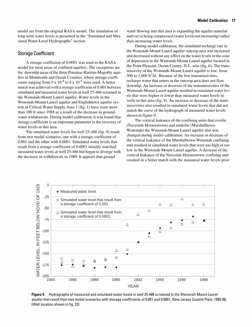
A storage coefficient of 0.0001 was used in the RASA model for most areas of confined aquifers. The exceptions are the downdip areas of the three Potomac-Raritan-Magothy aqui­fers in Monmouth and Ocean Counties, where storage coeffi­cients ranging from 5 x 10-4 to 8 x 10-4 were used. A better match was achieved with a storage coefficient of 0.001 between simulated and measured water levels at well 25-486 screened in the Wenonah-Mount Laurel aquifer. Water levels in the Wenonah-Mount Laurel aquifer and Englishtown aquifer sys­tem in Critical Water Supply Area 1 (fig. 1) have risen more than 100 ft since 1988 as a result of the decrease in ground­water withdrawals. During model calibration, it was found that storage coefficient is an important parameter in the recovery of water levels in this area.

The simulated water levels for well 25-486 (fig. 9) result from two model scenarios, one with a storage coefficient of 0.001 and the other with 0.0001. Simulated water levels that result from a storage coefficient of 0.0001 initially matched measured water levels at well 25-486 but began to diverge with the decrease in withdrawals in 1989. It appears that ground

water flowing into this area is expanding the aquifer material and (or) is being compressed (water levels not increasing) rather than increasing water levels.

During model calibration, the simulated recharge rate in the Wenonah-Mount Laurel aquifer outcrop area was increased and decreased without any effect on the water levels in the cone of depression in the Wenonah-Mount Laurel aquifer located in the Point Pleasant, Ocean County, N.J., area (fig. 6). The trans­missivity of the Wenonah-Mount Laurel aquifer is low, from 500 to 1,000 ft2/d. Because of the low transmissivities, recharge water that enters at the outcrop area does not flow downdip. An increase or decrease of the transmissivities of the Wenonah-Mount Laurel aquifer resulted in simulated water lev­els that were higher or lower than measured water levels in wells in this area (fig. 9). An increase or decrease of the trans­missivities also resulted in simulated water levels that did not match the curve of the hydrograph of measured water levels shown in figure 9.

The vertical leakance of the confining units that overlie (Navesink-Hornerstown) and underlie (Marshalltown-Wenonah) the Wenonah-Mount Laurel aquifer also was changed during model calibration. An increase or decrease of the vertical leakance of the Marshalltown-Wenonah confining unit resulted in simulated water levels that were too high or too low in the Wenonah-Mount Laurel aquifer. A decrease of the vertical leakance of the Navesink-Hornerstown confining unit resulted in a better match with the measured water levels prior

WA

TE

R L

EV

EL,

IN F

EE

T B

ELO

W N

GV

D O

F 1

929

-25

-50

-75

-100

-125

-150

-175

-200

0

Measured water level

Simulated water level that result from

Simulated water level that result from

a storage coefficient of 0.001

a storage coefficient of 0.0001

1984 1986 1988 1990 1992 1994 1996 1998

YEAR

Figure 9. Hydrographs of measured and simulated water levels in well 25-486 screened in the Wenonah-Mount Laurel aquifer that result from two model scenarios with storage coefficients of 0.001 and 0.0001, New Jersey Coastal Plain, 1985-98. (Well location shown in fig. 22)

18 Documentation of Revisions to the Regional Aquifer System Analysis Model of the New Jersey Coastal Plain

to the decrease in ground-water withdrawals that began in 1989. Simulated water levels after 1990 for the scenario with a storage coefficient of 0.0001 were as much as 83 ft higher than mea­sured water levels (1991). Again, all of these simulations resulted in water levels that did not match the curve of the hydrograph of measured water levels shown in figure 9. The measured water levels in well 25-486 have been increasing since 1989 (fig. 9), which indicates that water levels have not reached steady-state conditions.

Boundary Fluxes

To simulate the eastern part of a regional cone of depres­sion that has developed around wells in the Lower Potomac-Raritan-Magothy aquifer in Delaware, boundary fluxes near the Delaware and New Jersey State line were adjusted during model calibration until a reasonable match was achieved between the measured and simulated water levels in this area in 1998. The fluxes at this boundary were increased 0.5 Mgal/d from the 4.1 Mgal/d used in the original RASA model for the Lower Potomac-Raritan-Magothy aquifer. An increase of 0.5 Mgal/d at this boundary is less than 0.001 percent of the outflow of the entire model area for 1995.

The total 1997 ground-water withdrawals from the Lower Potomac-Raritan-Magothy aquifer in Delaware was 5.42 Mgal/d (Lacombe and Rosman, 2001). The location of these withdrawal wells shown in figure 10 is just beyond the active model area. The increased boundary fluxes at the Dela-ware-New Jersey boundary represent part of the ground-water withdrawals from these wells.

Simulated Potentiometric Surfaces

During model calibration, the simulated potentiometric surfaces were compared to those from each of the five Coastal Plain synoptic studies conducted in 1978, 1983, 1988, 1993, and 1998 to ensure that cones of depressions and flow directions were simulated throughout the time periods of the study. Dis­cussion of the potentiometric surfaces in this report is limited to 1978 and 1998 ground-water-flow conditions. The interpreted 1978 potentiometric surfaces also were compared to simulated transient-model results to ensure that the same level of calibra­tion was maintained or improved with the revised model. Hydrologic conditions for 1998 are discussed in this report because the 1998 water-level synoptic study provides the most recent water-level data.

1978 Ground-Water-Flow Conditions

In most areas of each aquifer the interpreted and simulated 1978 potentiometric surfaces compare well, and the level of cal­ibration was maintained or improved. Martin (1998) presents a lengthy discussion of the comparison of the simulated and inter­preted potentiometric surfaces, which still is valid for the revised model.

The simulated potentiometric surfaces from the RASA model and the revised model also compare well. The only minor difference in the calibration of the two models is in the cone of depression centered in Point Pleasant, N.J., in the Wenonah-Mount Laurel aquifer and Englishtown aquifer system. The revised model simulates the potentiometric surfaces in the cone of depression in this area to be about 20 and 40 ft, respectively, deeper than those of the RASA model. The 1978 interpreted potentiometric surfaces (potentiometric surfaces constructed with measured water levels) in the cones (Walker, 1983) in this area are about 180 and 240 ft below NGVD of 1929, respec­tively; these potentiometric surfaces compare well with the sim­ulated potentiometric surfaces from the revised model (fig. 11), which are about 160 and 220 ft below NGVD of 1929, respec­tively. The improvement in the agreement of water levels is because of the smaller grid spacing and the change in the verti­cal leakance values of the confining unit overlying the Wenonah-Mount Laurel aquifer.

1998 Ground-Water-Flow Conditions

The simulated and, when available, interpreted potentio­metric surfaces for 1998 are shown in figures 12-21. During the 1998 Coastal Plain water-level synoptic study (Lacombe and Rosman, 2001), no water levels were measured in the Holly Beach water-bearing zone, upper Kirkwood-Cohansey aquifer system, or Vincentown aquifer. In general, the interpreted and simulated water levels match closely; in most areas they are within 20 ft. The exceptions are in the cone of depression in the Piney Point, Wenonah-Mount Laurel, and Upper Potomac-Raritan-Magothy aquifers.

Water levels in the Piney Point aquifer simulated with the RASA model matched measured water levels closely except in the southwestern Coastal Plain and along the Atlantic Coast (Martin, 1998). Martin states that there were few measured water levels available for the Piney Point aquifer and further calibration of the model in this area was not beneficial. Water-level data for the Piney Point aquifer still are sparse. The aquifer was not a focus of this current study, and no attempt was made to match measured and simulated water levels with the revised model more closely. The same level of calibration is main­tained, however. The maximum difference (40 ft) between 1998 simulated and measured water levels is in the small cone of depression centered near Barnegat Light, N.J. (fig. 15).

The shape and depth of the two small cones of depression located in the Wenonah-Mount Laurel aquifer in Burlington County were not simulated as closely to measured water levels as those in other areas of the aquifer (fig. 17). The difference between the measured and simulated water levels in the cone of depression in northwestern Burlington County is about 40 ft. The difference between the measured and simulated water lev­els in the cone of depression in northeastern Burlington County is about 20 ft. The poor match between the simulated and mea­sured water levels could be due to contouring style and (or)

19 Model Calibration

75 53’42" 75 46’39" 75 39’36" 75 32’33" 75 25’30" 75 18’27"

39 50’ 15"

39 43’ 12"

39 36’ 09"

39 29’ 06"

NEW JERSEY

MA

RY

LAN

D

DE

LAW

AR

E

DE

LAW

AR

ER

IVER

DELAWARE BAY

PENNSYLVANIA

Base from U.S. Geological Survey digital data,1:100,000, 1983, Universal Transverse MecatorProjection, Zone 18 0 4 8 MILES

0 10 KILOMETERS

EXPLANATION

Location of ground-water withdrawl well

Figure 10. Location of ground-water withdrawal wells screened in the Lower Potomac-Raritan-Magothy aquifer in Delaware, 1997.

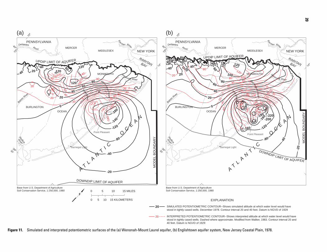
PENNSYLVANIA

MERCERMIDDLESEX

MONMOUTH

NEW YORK

AT

LA

NT

I C O

CE

AN

RARITANBAY

Base from U.S. Department of AgricultureSoil Conservation Service, 1:250,000, 1980

DelawareRiver

Rar i tan River

Naves ink RiverManasquan

River

Toms

River

Batsto

River

Mullica

BURLINGTON

OCEAN

75

3930’

40

75

74

Barnegat Light

River

Point Pleasant

MO

DE

L B

OU

ND

AR

Y

UPDIP LIMIT OF AQUIFER

DOWNDIP LIMIT OF AQUIFER

12040

20

100

4040 60

8060

40

20

0

-40

-120

-80

-160-200

-20

100

20

40 40

6060

4060

-160

-180

-180 -220

80

6040

20

-20

20

120

100

0

0-20

-40

-60

-80

-140

-100 -120

-180

-160

-200

80

-40 -180

-200

-220

-240

-60

0 5 10 15 MILES

0 5 10 15 KILOMETERS

-20

-40

-80

-120-140

-160

40 20

0

120

120

40 60 120

8060

40

20

0

12010080

60

40

2020

0

-2020

140

120

10080

0

0

-20-40-60

-80-1

40

-100

-120

-140 -160

-180

PENNSYLVANIA

MERCERMIDDLESEX

MONMOUTH

NEW YORK

AT

LA

NT

I C O

CE

AN

RARITANBAY

Base from U.S. Department of AgricultureSoil Conservation Service, 1:250,000, 1980

DelawareRiver

Rar i tan River

Naves ink RiverManasquan

River

Toms

River

Batsto

River

Mullica

BURLINGTON

OCEAN

SIMULATED POTENTIOMETRIC CONTOUR--Shows simulated altitude at which water level would have stood in tightly cased wells. December 1978. Contour interval 20 and 40 feet. Datum is NGVD of 1929

INTERPRETED POTENTIOMETRIC CONTOUR--Shows interpreted altitude at which water level would havestood in tightly cased wells. Dashed where approximate. Modified from Walker, 1983. Contour interval 20 and 40 feet. Datum is NGVD of 1929

EXPLANATION

75

3930’

40

75

74

20

20

Barnegat Light

River

Point Pleasant

(a) (b)

UPDIP LIMIT OF AQUIFER

DOWNDIP LIMIT OF AQUIFER

MO

DE

L B

OU

ND

AR

Y

20

Figure 11. Simulated and interpreted potentiometric surfaces of the (a) Wenonah-Mount Laurel aquifer, (b) Englishtown aquifer system, New Jersey Coastal Plain, 1978.

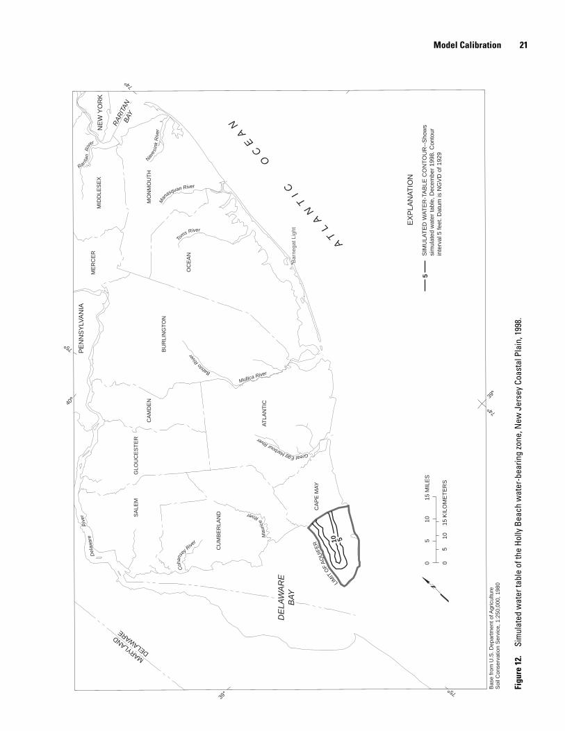
4

Model Calibration 21

5

74

0 5

10

15 M

ILE

S

0 5

10

15 K

ILO

ME

TE

RS

PE

NN

SY

LVA

NIA

ME

RC

ER

M

IDD

LES

EX

MO

NM

OU

TH

CA

MD

EN

GLO

UC

ES

TE

RS

ALE

M

AT

LAN

TIC

CA

PE

MA

Y

NE

W Y

OR

K

AT

LA

NT

IC

OC

EA

N

DE

LA W

AR

E

BA

Y

RA

RIT

AN

B

AY

Coh

ans e

y R i v e

r

Del

awar

e R

iver

R a r ita

n R

iv e r

Naves

ink

Riv

er

Ma n

a s q u a n R i v e r

To m s R i v e r

Batst

oRive

r

M u l li c a R i v e r

Mau

rice

River

GreatEggHarbourRiver

BU

RLI

NG

TO

N

OC

EA

N SIM

ULA

TE

D W

AT

ER

-TA

BLE

CO

NT

OU

R--

Sho

ws

sim

ulat

ed w

ater

tabl

e, D

ecem

ber

1998

. Con

tour

inte

rval

5 fe

et. D

atum

is N

GV

D o

f 192

9

EX

PLA

NA

TIO

N

MARYLAND

DELAWARE

75

39

40

7

7

39

5

Bar

nega

t Lig

ht

LIM

ITO

FA

QU

IFE

R

CU

MB

ER

LAN

D

510

Bas

e fr

om U

.S. D

epar

tmen

t of A

gric

ultu

reS

oil C

onse

rvat

ion

Ser

vice

, 1:2

50,0

00, 1

980

Figu

re 1

2.

Sim

ulat

ed w

ater

tabl

e of

the

Holly

Bea

ch w

ater

-bea

ring

zone

, New

Jer

sey

Coas

tal P

lain

, 199

8.

5

0 5

10

15 M

ILE

S

0 5

10

15 K

ILO

ME

TE

RS

-10

0

0

0

0 0

0

0

0 20

0

060

100

120

60

60

140

100

120

60

20

20

0

60

100

140

60

60

PE

NN

SY

LVA

NIA

ME

RC

ER

M

IDD

LES

EX

MO

NM

OU

TH

CA

MD

EN

GLO

UC

ES

TE

RS

ALE

M

AT

LAN

TIC

CA

PE

MA

Y

NE

W Y

OR

K

AT

LA

NT

IC

OC

EA

N

DE

LA W

AR

E

BA

Y

RA

RIT

AN

B

AY

Coh

an s e

y R i v e

r

Del

awar

e R

iver

R a r ita

n R

iv e r

N a v

esin

k R

iver

M

a n a s q u a n R i v e r

T o m s R i v e r

Batst

oRive

r

M u l li c a R i v e r

Mau

rice

River

GreatEggHarbourRiver

BU

RLI

NG

TO

N

OC

EA

N SIM

ULA

TE

D W

AT

ER

TA

BLE

CO

NT

OU

R--

Sho

ws

altit

ude

of s

imul

ated

wat

er ta

ble

and

pote

ntio

met

ricsu

rfac

e D

ecem

ber

1998

. Con

tour

inte

rval

is v

aria

ble.

Dat

um is

NG

VD

of 1

929

EX

PLA

NA

TIO

N

MARYLAND

DELAWARE

75

39

40

7

74

39

20

Bar

nega

t Lig

ht

MODEL BOUNDARY

UP

DIP

LIM

IT O

F O

VE

RLY

ING

CO

NF

ININ

G U

NIT

UP

DIP

LIM

IT O

F A

QU

IFE

R

CU

MB

ER

LAN

D

22 Documentation of Revisions to the Regional Aquifer System Analysis Model of the New Jersey Coastal Plain

Bas

e fr

om U

.S. D

epar

tmen

t of A

gric

ultu

reS

oil C

onse

rvat

ion

Ser

vice

, 1:2

50,0

00, 1

980

74

Figu

re 1

3.

Sim

ulat

ed w

ater

tabl

e an

d si

mul

ated

pot

entio

met

ric s

urfa

ces

of th

e up

per K

irkw

ood-

Coha

nsey

aqu

ifer s

yste

m, N

ew J

erse

y Co

asta

l Pla

in, 1

998.

Model Calibration 23

5

0 5

10

15 M

ILE

S

0 5

10

15 K

ILO

ME

TE

RS

0

20

60

120

60

60

60

60

60

0

20

0

-20 -4

0 -8

0

-70 -6

0 -50

-40

120

0

-20

60140 12

0 10

0

180

160

140

120

140

10012

0 14

0

60

60

60

140

0

0

100

100

20

60

0

-40

-60

-100

-80

-60

-40

-20

0

0 20

PE

NN

SY

LVA

NIA

ME

RC

ER

M

IDD

LES

EX

MO

NM

OU

TH

CA

MD

EN

GLO

UC

ES

TE

RS

ALE

M

AT

LAN

TIC

CA

PE

MA

Y

NE

W Y

OR

K

AT

LA

NT

IC

OC

EA

N

DE

LA W

AR

E

BA

Y

RA

RIT

AN

B

AY

Coh

an s e y R

i v e r

Del

awar

e R

iver

R a r ita

n R

iv e r

N a v

esin

k R

iver

M

a n a s q u a n R i v e r

T o m s R i v e r

Batst

oRive

r

M u l li c a R i v e r

Mau

rice

River

GreatEggHarbourRiver

BU

RLI

NG

TO

N

OC

EA

N SIM

ULA

TE

D P

OT

EN

TIO

ME

TR

IC C

ON

TO

UR

--S

how

ssi

mul

ated

alti

tude

at w

hich

wat

er le

vel w

ould

hav

est

ood

in ti

ghtly

cas

ed w

ells

. Dec

embe

r 19

98. C

onto

urin

terv

al 2

0 fe

et. D

atum

is N

GV

D o

f 192

9

INT

ER

PR

ET

ED

PO

TE

NT

IOM

ET

RIC

CO

NT

OU

R--

Sho

ws

inte

rpre

ted

altit

ude

at w

hich

wat

er le

vel w

ould

hav

est

ood

in ti

ghtly

cas

ed w

ells

. Das

hed

whe

re a

ppro

xim

ate.

Mod

ified

from

Lac

ombe

and

Ros

man

, 200

1. C

onto

urin

terv

al 2

0 fe

et. D

atum

is N

GV

D o

f 192

9

EX

PLA

NA

TIO

N

MARYLAND

DELAWARE

75

39

40

7

74

39

20 20 B

arne

gat L

ight

UP

DIP

LIM

IT O

F A

QU

IFE

RMODEL BOUNDARY

UPDIPLI

MIT

OF

OV

ER

LYIN

GC

ON

FIN

ING

UN

IT

CU

MB

ER

LAN

D

Bas

e fr

om U

.S. D

epar

tmen

t of A

gric

ultu

reS

oil C

onse

rvat

ion

Ser

vice

, 1:2

50,0

00, 1

980

74

Figu

re 1

4.

Siim

ulat

ed a

nd in

terp

rete

d po

tent

iom

etric

sur

face

s of

the

low

er K

irkw

ood-

Coha

nsey

aqu

ifer s

yste

m a

nd c

onfin

ed K

irkw

ood

aqui

fer,

New

Jer

sey

Coas

tal P

lain

, 199

8.

24

5

74

0 5

10

15 M

ILE

S

0 5

10

15 K

ILO

ME

TE

RS

PE

NN

SY

LVA

NIA

ME

RC

ER

M

IDD

LES

EX

MO

NM

OU

TH

CA

MD

EN

GLO

UC

ES

TE

RS

ALE

M

AT

LAN

TIC

CA

PE

MA

Y

NE

W Y

OR

K

AT

LA

NT

IC

OC

EA

N

DE

LA W

AR

E

BA

Y

RA

RIT

AN

B

AY

Coh

an s e

y R i v e

r

Del

awar

e R

iver

R a r ita

n R

iv e r

N a v

esin

k R

iver

M

a n a s q u a n R i v e r

T o m s R i v e r

Batst

oRive

r

M u l li c a R i v e r

Mau

rice

River

GreatEggHarbourRiver

BU

RLI

NG

TO

N

OC

EA

N

SIM

ULA

TE

D P

OT

EN

TIO

ME

TR

IC C

ON

TO

UR

--S

how

ssi

mul

ated

alti

tude

at w

hich

wat

er le

vel w

ould

hav

est

ood

in ti

ghtly

cas

ed w

ells

. Dec

embe

r 19

98. C

onto

urin

terv

al 2

0 fe

et. D

atum

is N

GV

D o

f 192

9

INT

ER

PR

ET

ED

PO

TE

NT

IOM

ET

RIC

CO

NT

OU

R--

Sho

ws

inte

rpre

ted

altit

ude

at w

hich

wat

er le

vel w

ould

hav

est

ood

in ti

ghtly

cas

ed w

ells

. Das

hed

whe

re a

ppro

xim

ate.

Mod

ified

from

Lac

ombe

and

Ros

man

, 199

8. C

onto

urin

terv

al 2

0 fe

et. D

atum

is N

GV

D o

f 192

9

EX

PLA

NA

TIO

N

MARYLAND

DELAWARE

75

39

40

7

7

39

20 20

Bar

nega

t Lig

ht

CU

MB

ER

LAN

D

MO

DE

L B

OU

ND

AR

Y

DO

WN

DIP

LIM

IT O

F A

QU

IFE

R

UP

DIP

LIM

ITO

FA

QU

IFE

R

60

100 80

-20

40

60

120

20

0

-60

-40

-20

-20

-20

-40-60

-20

-20

0

60

40 20

0

-20

0

-20

-40

-40

-20

-60

120

100 80

60

-40

-60

Bas

e fr

om U

.S. D

epar

tmen

t of A

gric

ultu

reS

oil C

onse

rvat

ion

Ser

vice

, 1:2

50,0

00, 1

980

Figu

re 1

5.

Sim

ulat

ed a

nd in

terp

rete

d po

tent

iom

etric

sur

face

s of

the

Pine

y Po

int a

quife

r, N

ew J

erse

y Co

asta

l Pla

in, 1

998.

4

Documentation of Revisions to the Regional Aquifer System Analysis Model of the New Jersey Coastal Plain

4

Model Calibration 25

5

74

0 5

10

15 M

ILE

S

0 5

10

15 K

ILO

ME

TE

RS

40

60

40

20

1010

10

60 80

100

8060

40

40

20

40

120

100

40

6080

80 100

12016

0 14

0

120

80100

60

40 20

100

80

80 60

20

10

60

40

20

140

100

120

100

80

60

80 60

40

100

80

PE

NN

SY

LVA

NIA

ME

RC

ER

M

IDD

LES

EX

MO

NM

OU

TH

CA

MD

EN

GLO

UC

ES

TE

R

SA

LEM

AT

LAN

TIC

CA

PE

MA

Y

NE

W Y

OR

K

AT

LA

NT

IC

OC

EA

N

DE

LA W

AR

E

BA

Y

RA

RIT

AN

B

AY

Coh

an s e y R

i v e r

Del

awar

e R

iver

R a r ita

n R

iv e r

N a v

esin

k R

iver

M

a n a s q u a n R i v e r

T o m s R i v e r

Batst

oRive

r

M u l li c a R i v e r

Mau

rice

River

GreatEggHarbourRiver

BU

RLI

NG

TO

N

OC

EA

N S

IMU

LAT

ED

PO

TE

NT

IOM

ET

RIC

CO

NT

OU

R--

Sho

ws

sim

ulat

ed a

ltitu

de a

t whi

ch w

ater

leve

l wou

ld h

ave

stoo

d in

tigh

tly c

ased

wel

ls. D

ecem

ber

1998

. Con

tour

inte

rval

20

feet

. Dat

um is

NG

VD

of 1

929

INT

ER

PR

ET

ED

PO

TE

NT

IOM

ET

RIC

CO

NT

OU

R--

Sho

ws

inte

rpre

ted

altit

ude

at w

hich

wat

er le

vel w

ould

hav

est

ood

in ti

ghtly

cas

ed w

ells

. Das

hed

whe

re a

ppro

xim

ate.

Mod

ified

from

Lac

ombe

and

Ros

man

, 199

8. C

onto

urin

terv

al 2

0 fe

et. D

atum

is N

GV

D o

f 192

9

EX

PLA

NA

TIO

N

MARYLAND

DELAWARE

75

39

40

7

7

39

20 20

Bar

nega

t Lig

ht

MO

DE

L B

OU

ND

AR

Y

DO

WN

DIP

LIM

IT O

F A

QU

IFE

R

UP

DIP

LIM

IT O

F A

QU

IFE

R

CU

MB

ER

LAN

D

Bas

e fr

om U

.S. D

epar

tmen

t of A

gric

ultu

reS

oil C

onse

rvat

ion

Ser

vice

, 1:2

50,0

00, 1

980

Figu

re 1

6.

Sim

ulat

ed a

nd in

terp

rete

d po

tent

iom

etric

sur

face

s of

the

Vinc

ento

wn

aqui

fer,

New

Jer

sey

Coas

tal P

lain

, 199

8.

26 Documentation of Revisions to the Regional Aquifer System Analysis Model of the New Jersey Coastal Plain

5

0 5

10

15 M

ILE

S

0 5

10

15 K

ILO

ME

TE

RS

PE

NN

SY

LVA

NIA

ME

RC

ER

M

IDD

LES

EX

MO

NM

OU

TH

CA

MD

EN

GLO

UC

ES

TE

R

SA

LEM

AT

LAN

TIC

CA

PE

MA

Y

NE

W Y

OR

K

AT

LA

NT

IC

OC

EA

N

DE

LA W

AR

E

BA

Y

RA

RIT

AN

B

AY

Coh

an s e

y R i v e

r

Del

awar

e R

iver

R a r ita

n R

iv e r

N a v

esin

k R

iver

M

a n a s q u a n R i v e r

T o m s R i v e r

Batst

oRive

r

M u l li c a R i v e r

Mau

rice

River

GreatEggHarbourRiver

BU

RLI

NG

TO

N

OC

EA

N

SIM

ULA

TE

D P

OT

EN

TIO

ME

TR

IC C

ON

TO

UR

--S

how

ssi

mul

ated

alti

tude

at w

hich

wat

er le

vel w

ould

hav

est

ood

in ti

ghtly

cas

ed w

ells

. Dec

embe

r 19

98. C

onto

urin

terv

al 2

0 fe

et. D

atum

is N

GV

D o

f 192

9

INT

ER

PR

ET

ED

PO

TE

NT

IOM

ET

RIC

CO

NT

OU

R--

Sho

ws

inte

rpre

ted

altit

ude

at w

hich

wat

er le

vel w

ould

hav

est

ood

in ti

ghtly

cas

ed w

ells

. Das

hed

whe

re a

ppro

xim

ate.

Mod

ified

from

Lac

ombe

and

Ros

man

, 199

8. C

onto

urin

terv

al 2

0 fe

et. D

atum

is N

GV

D o

f 192

9

EX

PLA

NA

TIO

N

MARYLAND

DELAWARE

75

39

40

7

74

39

20 20 B

arne

gat L

ight

MO

DE

L B

OU

ND

AR

Y

UP

DIP

LIM

IT O

F A

QU

IFE

R

DO

WN

DIP

LIM

IT O

F A

QU

IFE

R

CU

MB

ER

LAN

D

0

40

40

40

20

20

40

40

20 0

3020

2060

40 80

60 40

20

20

40

60

120

100

120

100

80

60

0

0

20

40

-20 -3

0

-40

-40 -5

0

-50 -60

-80

00

60

60

-40 -2

0 -6

0-4

040

20

-20 -4

0 0

60

80

120

100

60

20

-20

0

140

120

100

80 60

40 20

0

-20

-40

-60-8

0 -8

0

Bas

e fr

om U

.S. D

epar

tmen

t of A

gric

ultu

reS

oil C

onse

rvat

ion

Ser

vice

, 1:2

50,0

00, 1

980

74

Figu

re 1

7.

Sim

ulat

ed a

nd in

terp

rete

d po

tent

iom

etric

sur

face

s of

the

Wen

onah

-Mou

nt L

aure

l aqu

ifer,

New

Jer

sey

Coas

tal P

lain

, 199

8.

Model Calibration 27

5

0 5

10

15 M

ILE

S

0 5

10

15 K

ILO

ME

TE

RS

PE

NN

SY

LVA

NIA

M

ER

CE

R

MID

DLE

SE

X

MO

NM

OU

TH

CA

MD

EN

GLO

UC

ES

TE

R

SA

LEM

AT

LAN

TIC

CA

PE

MA

Y

NE

W Y

OR

K

AT

LA

NT

IC

OC

EA

N

DE

LA W

AR

E

BA

Y

RA

RIT

AN

B

AY

Coh

an s e

y R i v e

r

Del

awar

e R

iver

Rari ta

n R

iver

N a v

e sin

k R

iver

M

a n a s q u a n R i v e r

T o m s R i v e r

Batst

oRive

r

M u l li c a R i v e r

Mau

rice

River

Grea tEggHarbourRiver

BU

RLI

NG

TO

N

OC

EA

N

SIM

ULA

TE

D P

OT

EN

TIO

ME

TR

IC C

ON

TO

UR

--S

how

ssi

mul

ated

alti

tude

at w

hich

wat

er le

vel w

ould

hav

est

ood

in ti

ghtly

cas

ed w

ells

. Dec

embe

r 19

98. C

onto

urin

terv

al 2

0 fe

et. D

atum

is N

GV

D o

f 192

9

INT

ER

PR

ET

ED

PO

TE

NT

IOM

ET

RIC

CO

NT

OU

R--

Sho

ws

inte

rpre

ted

altit

ude

at w

hich

wat

er le

vel w

ould

hav

est

ood

in ti

ghtly

cas

ed w

ells

. Das

hed

whe

re a

ppro

xim

ate.

Mod

ified

from

Lac

ombe

and

Ros

man

, 199

8. C

onto

urin

terv

al 2

0 fe

et. D

atum

is N

GV

D o

f 192

9

EX

PLA

NA

TIO

N

MARYLAND

DELAWARE

75

39

40

7

74

39

20 20

Bar

nega

t Lig

ht

MO

DE

L B

OU

ND

AR

Y

UP

DIP

LIM

IT O

F A

QU

IFE

R

DO

WN

DIP

LI M

IT O

F A

QU

IFE

R

CU

MB

ER

LAN

D 40

20 40

20

402020

40

40

40

20

60 40

200 60

60

60

0

40

60 40

20

40

40 40

60

40

60

120

100

100

80

60

40

20

0

-20

-40

-60

-80

-100

80

80

0 60

40

20

80

0

0 60

40

20

40

40

100

8060

20

0 -2

0 -40

-80

-60

-100

-80

-100

Bas

e fr

om U

.S. D

epar

tmen

t of A

gric

ultu

reS

oil C

onse

rvat

ion

Ser

vice

, 1:2

50,0

00, 1

980

74

Figu

re 1

8.

Sim

ulat

ed a

nd in

terp

rete

d po

tent

iom

etric

sur

face

s of

the

Engl

isht

own

aqui

fe s

yste

m, N

ew J

erse

y Co

asta

l Pla

in, 1

998.

28 Documentation of Revisions to the Regional Aquifer System Analysis Model of the New Jersey Coastal Plain

5 0

5 10

15

MIL

ES

0 5

10

15 K

ILO

ME

TE

RS

PE

NN

SY

LVA

NIA

ME

RC

ER

M

IDD

LES

EX

MO

NM

OU

TH

CA

MD

EN

GLO

UC

ES

TE

RS

ALE

M

AT

LAN

TIC

CA

PE

MA

Y

NE

W Y

OR

K

AT

LA

NT

IC

OC

EA

N

DE

LA W

AR

E

BA

Y

RA

RIT

AN

B

AY

Coh

an s e

y R i v e

r

Del

awar

e R

iver

R a r ita

n R

iv e r

N a v

esin

k R

iver

M

a n a s q u a n R i v e r

T o m s R i v e r

Batst

oRive

r

M u l li c a R i v e r

Mau

rice

River

GreatEggHarbourRiver

BU

RLI

NG

TO

N

OC

EA

N S

IMU

LAT

ED

PO

TE

NT

IOM

ET

RIC

CO

NT

OU

R--

Sho

ws

sim

ulat

ed a

ltitu

de a

t whi

ch w

ater

leve

l wou

ld h

ave

stoo

d in

tigh

tly c

ased

wel

ls. D

ecem

ber

1998

. Con

tour

inte

rval

20

feet

. Dat

um is

NG

VD

of 1

929

INT

ER

PR

ET

ED

PO

TE

NT

IOM

ET

RIC

CO

NT

OU

R--

Sho

ws

inte

rpre

ted

altit

ude

at w

hich

wat

er le

vel w

ould

hav

est

ood

in ti

ghtly

cas

ed w

ells

. Das

hed

whe

re a

ppro

xim

ate.

Mod

ified

from

Lac

ombe

and

Ros

man

, 199

8. C

onto

urin

terv

al 2

0 fe

et. D

atum

is N

GV

D o

f 192

9

EX

PLA

NA

TIO

N

MARYLAND

DELAWARE

75

39

40

7

74

39

20 20

Bar

nega

t Lig

ht

MO

DE

L B

OU

ND

AR

Y

UP

DIP

LIM

IT O

F A

QU

IFE

R

CU

MB

ER

LAN

D

AP

PR

OX

IMA

TE

SE

AW

AR

D L

IMIT

OF

FR

ES

HW

AT

ER

IN

LOW

ER

PO

TO

MA

C-R

AR

ITA

N-M

AG

OT

HY

AQ

UIF

ER

AS

DE

LIN

EA

TE

D B

Y C

HLO

RID

E C

ON

CE

NT

RA

TIO

N

OF

10,

000

MIL

LIG

RA

MS

PE

R L

ITE

R

0 0

0

-50

-60

-70 -70-4

0 80

60

40

20

20 0

60

40

0

-20

-40

-40

-40

-20

-20

0

-20

-60

-80

-80

-100

-40

-40

-20

0

0

-20

60

40

20

0

-20

-20

-60

-20

Bas

e fr

om U

.S. D

epar

tmen

t of A

gric

ultu

reS

oil C

onse

rvat

ion

Ser

vice

, 1:2

50,0

00, 1

980

74

Figu

re 1

9.

Sim

ulat

ed a

nd in

terp

rete

d po

tent

iom

etric

sur

face

s of

the

Uppe

r Pot

omac

-Rar

itan-

Mag

othy

aqu

ifer,

New

Jer

sey

Coas

tal P

lain

, 199

8.

Model Calibration 29

5

0 5

10

15 M

ILE

S

0 5

10

15 K

ILO

ME

TE

RS

PE

NN

SY

LVA

NIA

ME

RC

ER

MID

DLE

SE

X

MO

NM

OU

TH

CA

MD

EN

GLO

UC

ES

TE

RS

ALE

M

AT

LAN

TIC

CA

PE

MA

Y

NE

W Y

OR

K

AT

LA

NT

IC

OC

EA

N

DE

LA W

AR

E

BA

Y

RA

RIT

AN

B

AY

Coh

an s e y R

i v e r

Del

awar

e R

iver

R a r ita

n R

iv e r

N a v

esin

k R

iver

M

a n a s q u a n R i v e r

T o m s R i v e r

Batst

oRive

r

M u l li c a R i v e r

Mau

rice

River

GreatEggHarbourRiver

BU

RLI

NG

TO

N

OC

EA

N

SIM

ULA

TE

D P

OT

EN

TIO

ME

TR

IC C

ON

TO

UR

--S

how

ssi

mul

ated

alti

tude

at w

hich

wat

er le

vel w

ould

hav

est

ood

in ti

ghtly

cas

ed w

ells

. Dec

embe

r 19

98. C

onto

urin

terv

al 2

0 fe

et. D

atum

is N

GV

D o

f 192

9

INT

ER

PR

ET

ED

PO

TE

NT

IOM

ET

RIC

CO

NT

OU

R--

Sho

ws

inte

rpre

ted

altit

ude

at w

hich

wat

er le

vel w

ould

hav

est

ood

in ti

ghtly

cas

ed w

ells

. Das

hed

whe

re a

ppro

xim

ate.

Mod

ified

from

Lac

ombe

and

Ros

man

, 199

8. C

onto

urin

terv

al 2

0 fe

et. D

atum

is N

GV

D o

f 192

9

EX

PLA

NA

TIO

N

MARYLAND

DELAWARE

75

40

7

74

39

20 20

Bar

nega

t Lig

ht

CU

MB

ER

LAN

D

MO

DE

L B

OU

ND

AR

Y

UP

DIP

LIM

IT O

F A

QU

IFE

R

AP

PR

OX

IMA

TE

SE

AW

AR

D L

IMIT

OF

FR

ES

HW

AT

ER

IN

LOW

ER

PO

TO

MA

C-R

AR

ITA

N-M

AG

OT

HY

AQ

UIF

ER

A

S D

ELI

NE

AT

ED

BY

CH

LOR

IDE

CO

NC

EN

TR

AT

ION

O

F 1

0,00

0 M

ILLI

GR

AM

S P

ER

LIT

ER

-20

-40

-20

-20

-20

-50

-60

-40

0

-20

20

40

6040

80

80

100 80

60

60

40

20

20

-40

60

40

20

-40

-20

-40

-20

-60

-40

-60

-60

0

0

20

40

60

-20

-20

-40

-20

0

-20

74

Bas

e fr

om U

.S. D

epar

tmen

t of A

gric

ultu

reS

oil C

onse

rvat

ion

Ser

vice

, 1:2

50,0

00, 1

980

Figu

re 2

0.

Sim

ulat

ed a

nd in

terp

rete

d po

tent

iom

etric

sur

face

s of

the

Mid

dle

Poto

mac

-Rar

itan-

Mag

othy

aqu

ifer,

New

Jer

sey

Coas

tal P

lain

, 199

8.

39

5

30 Documentation of Revisions to the Regional Aquifer System Analysis Model of the New Jersey Coastal Plain

4

0 5

10

15 M

ILE

S

0 5

10

15 K

ILO

ME

TE

RS

PE

NN

SY

LVA

NIA

ME

RC

ER

M

IDD

LES

EX

MO

NM

OU

TH

CA

MD

EN

GLO

UC

ES

TE

R

SA

LEM

AT

LAN

TIC

CA

PE

MA

Y

NE

W Y

OR

K

AT

LA

NT

IC

OC

EA

N

DE

LA W

AR

E

BA

Y

RA

RIT

AN

B

AY

Coh

an s e

y R i v e

r

Del

awar

e R

iver

R a r ita

n R

iv e r

N a v

esin

k R

iver

M

a n a s q u a n R i v e r

T o m s R i v e r

Batst

oRive

r

M u l li c a R i v e r

Mau

rice

River

GreatEggHarbourRiver

BU

RLI

NG

TO

N

OC

EA

N

SIM

ULA

TE

D P

OT

EN

TIO

ME

TR

IC C

ON

TO

UR

--S

how

ssi

mul

ated

alti

tude

at w

hich

wat

er le

vel w

ould

hav

est

ood

in ti

ghtly

cas

ed w

ells

. Dec

embe

r 19

98. C

onto

urin

terv

al 2

0 fe

et. D

atum

is N

GV

D o

f 192

9

INT

ER

PR

ET

ED

PO

TE

NT

IOM

ET

RIC

CO

NT

OU

R--

Sho

ws

inte

rpre

ted

altit

ude

at w

hich

wat

er le

vel w

ould

hav

est

ood

in ti

ghtly

cas

ed w

ells

. Das

hed

whe

re a

ppro

xim

ate.

Mod

ified

from

Lac

ombe

and

Ros

man

, 199

8. C

onto

urin

terv

al 2

0 fe

et. D

atum

is N

GV

D o

f 192

9

EX

PLA

NA

TIO

N

MARYLAND

DELAWARE

75

40

7

7

39

20

20

Bar

nega

t Lig

ht

CU

MB

ER

LAN

D

MO

DE

L B

OU

ND

AR

Y

UPDIP LIMIT OF AQUIFER

AP

PR

OX

IMAT

E S

EAW

AR

D L

IMIT

OF

FRE

SH

WAT

ER

IN

LOW

ER

PO

TOM

AC

-RA

RIT

AN

-MA

GO

THY

AQ

UIF

ER

AS

DE

LIN

EAT

ED

BY

CH

LOR

IDE

CO

NC

EN

TRAT

ION

OF

10,0

00 M

ILLI

GR

AM

S P

ER

LIT

ER

-60

-50

-40

-20

0 0

-40-50

-60

-80

-20

-20

-40

-60

-40

-60-80

-120

-100

-20

-20

Bas

e fr

om U

.S. D

epar

tmen

t of A

gric

ultu

reS

oil C

onse

rvat

ion

Ser

vice

, 1:2

50,0

00, 1

980

74

Figu

re 2

1.

Sim

ulat

ed a

nd in

terp

rete

d po

tent

iom

etric

sur

face

s of

the

Low

er P

otom

ac-R

arita

n-M

agot

hy a

quife

r, N

ew J

erse

y Co

asta

l pla

in, 1

998.

39

unreported ground-water withdrawals. The NJDEP does not require that ground-water withdrawals less than 100,000 gal/d be reported. The Wenonah-Mount Laurel aquifer has low trans­missivity values (500 to 1,000 ft2/d), and during model calibra­tion, water levels in the aquifer were found to be sensitive to ground-water withdrawals. Unreported ground-water with­drawals that are not simulated in the model could cause simu­lated water levels to be higher than measured levels.

The simulated water levels in the Upper Potomac-Raritan-Magothy aquifer are as much as 35 ft higher than measured water levels in the cone of depression centered in Camden County (fig. 19). The 1998 simulated water levels were within 10 and 15 ft of measured water levels in wells 5-258 and 7-477 (fig. 22), respectively, which are located on the flanks of this regional cone of depression. Water levels in well 5-258 initially were simulated more closely, within 3 ft of the measured water levels. The difference between the simulated and measured water levels increased beginning in 1983. Determining the spe­cific cause of these differences is beyond the scope of this study.

Simulated and Measured Water-Level Hydrographs

Long-term hydrographs were plotted for the 28 selected wells shown in figure 22; these hydrographs were used during model calibration. The wells were selected on the basis of loca­tion and period of record. Also, when possible, wells used by Martin (1998) were selected. Some of the wells with hydro-graphs that Martin used during model calibration are no longer monitored; when possible, a nearby well, for which a hydrograph is available, was selected.

Hydrographs of simulated and measured water levels for the 28 wells are shown in figures 23-49. In general, the simu­lated water levels are within 25 ft of the measured water levels and, in most cases, are within 5 ft.

Wells 1-834, 7-283, 7-477, 7-478, 11-96, and 33-251, which have the greatest differences between simulated and measured water levels, are located near regional cones of depression (fig. 22). The large differences between the simu­lated and measured water levels could be due to the discretiza­tion scale of the model area and (or) unreported ground-water withdrawals. Simulated water levels are an average for each model cell.

Differences in measured water levels among aquifers were compared to differences in simulated water levels at five well clusters located throughout the New Jersey Coastal Plain. The location of well clusters is shown in figure 22. Each well cluster consists of at least two wells in close proximity, screened in two different aquifers. Three of the five well clusters consist of four wells in close proximity; one well is screened in the outcrop area of an aquifer where unconfined conditions are present, and the other three wells are screened in different confined aquifers. Evaluation of the water-level differences among aquifers showed that the direction of flow between confined aquifers and the water table is simulated accurately.

Model Calibration 31

Base Flow

The simulated and estimated base flows at continuous-record streamflow-gaging stations in the Toms River, North Branch Rancocas Creek, South Branch Rancocas Creek, Rac­coon Creek, and Salem River drainage basins are listed in table 4, and the location of the sites is shown in figure 6. These basins were selected because a detailed analysis of base flow was available for each of the rivers and because each river is repre­sentative of typical rivers in the New Jersey Coastal Plain. The estimated base-flow values listed in table 4 are the mean base flows for the time period shown in the table. The interval for the calculated mean base flow ranges from 26 to 68 years. The val­ues listed in table 4 for the simulated base flow are the average for the interval of the simulation, 1968–98, from the transient model. The base flow for each river and stress period was cal­culated. The values were added, then divided by 21, the number of stress periods. The resulting value is the simulated mean annual base flow.

The simulated and calculated mean base flow in the five river basins compare well; all differences are less than 31 per­cent. The simulated and calculated base flow at continuous-record streamflow gaging stations Toms River (01408500) and North Branch Rancocas Creek (01467000), the two large basins, match closely, within 10 percent. Differences are larger between the simulated and calculated base flow at Raccoon Creek (01477120) and Salem River (01482500), the two small basins, 31 and 27 percent, respectively.

Model Limitations

This revised model of the New Jersey Coastal Plain sedi­ments is a tool for analysis of the regional ground-water-flow system. All models are an approximation of the actual ground-water-flow system. Ground-water-flow models generally are based on conceptual models that are simplified representations of complex heterogeneous systems. Assumptions such as isot­ropy and vertical homogeneity within each layer are examples of simplified representation that can be a source of simulation errors. Local scale heterogeneities or hydrologic features not represented in the model may affect results. Model parameters were estimated in areas where there is a lack of data, such as water-level measurements. Model parameters, such as trans­missivity, ground-water withdrawals, and recharge rates, repre­sent averages for areas that range from 0.25 mi2 to 0.32 mi2. Local features, such as the maximum depth of a cone of depres­sion, are not simulated with the revised model. Water levels that result from seasonal variations in ground-water withdrawals or recharge rates also are not simulated.

32

5 0

5 10

15

MIL

ES

0 5

10

15 K

ILO

ME

TE

RS

PE

NN

SY

LVA

NIA

ME

RC

ER

M

IDD

LES

EX

MO

NM

OU

TH

CA

MD

EN

GLO

UC

ES

TE

RS

ALE

M

AT

LAN

TIC

CA

PE

MA

Y

NE

W Y

OR

K

AT

LA

NT

IC

OC

EA

N

DE

LA W

AR

E

BA

Y

RA

RIT

AN

B

AY

Coh

ans e

y R i v e

r

Del

awar

e R

iver

R a r ita

n R

iv e r

Naves

ink

Riv

er

Ma n

a s q u a n R i v e r To

m s R i v e r

Batst

oRive

r

M u l li c a R i v e r

Mau

rice

River

GreatEggHarbourRiver

BU

RLI

NG

TO

N

OC

EA

N

OB

SE

RV

AT

ION

WE

LL A

ND

WE

LL N

UM

BE

R--

Fig

ure

num

ber

in th

is r

epor

t for

mea

sure

d an

d si

mul

ated

hydr

ogra

ph is

sho

wn

in p

aren

thes

es

EX

PLA

NA

TIO

N

MARYLAND

DELAWARE

75

39

40

7

7

39

Bar

nega

t Lig

ht

CU

MB

ER

LAN

D

11-9

6(29

)

33-2

51(4

5) 33-1

87(4

7)

15-7

12(4

8)15

-713

(44)

15-7

28(4

1)

7-28

3(46

) 5-

258(

39)

5-25

9(38

)5-

261(

43)

5-26

2(49

)

7-47

7(40

)7-

478(

32)

5-67

6(27

)

29-1

38(3

5)29

-139

(29)

29-1

40(3

4)29

-141

(23)

25-6

36(3

0)25

-637

(33)

25-6

38(3

7)25

-639

(42)

25

-353

(31)

25-4

29(3

6)

25-4

86(9

)

1-57

8(24

) 1-83

4(26

)

1-37

(25)

11-9

6(28

)

4

Documentation of Revisions to the Regional Aquifer System Analysis Model of the New Jersey Coastal Plain

Bas

e fr

om U

.S. D

epar

tmen

t of A

gric

ultu

reS

oil C

onse

rvat

ion

Ser

vice

, 1:2

50,0

00, 1

980

74

Figu

re 2

2.

Loca

tion

of s

elec

ted

obse

rvat

ion

wel

ls fo

r whi

ch h

ydro

grap

hs o

f sim

ulat

ed a

nd m

easu

red

wat

er le

vels

hav

e be

en p

lotte

d, N

ew J

erse

y Co

asta

l Pla

in.

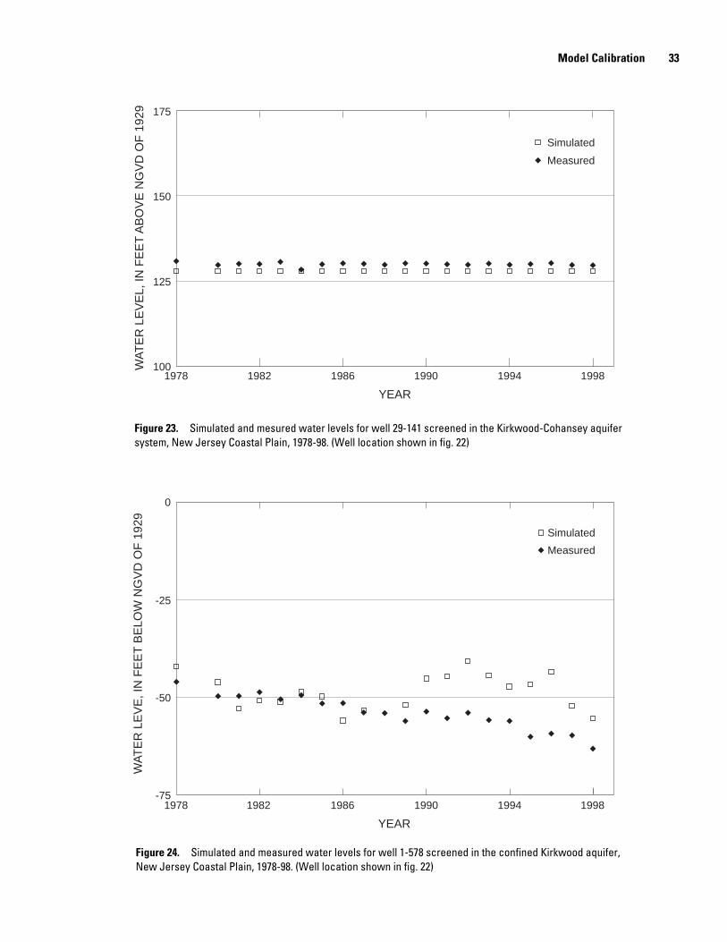
33 Model Calibration

100

125

150

1759

Measured

SimulatedW

AT

ER

LE

VE

L, IN

FE

ET

AB

OV

E N

GV

D O

F 1

92

1978 1982 1986 1990 1994 1998

YEAR

Figure 23. Simulated and mesured water levels for well 29-141 screened in the Kirkwood-Cohansey aquifer system, New Jersey Coastal Plain, 1978-98. (Well location shown in fig. 22)

-75

-50

-25

0

Measured

Simulated

WA

TE

R L

EV

E, I

N F

EE

T B

ELO

W N

GV

D O

F 1

929

1978 1982 1986 1990 1994 1998

YEAR

Figure 24. Simulated and measured water levels for well 1-578 screened in the confined Kirkwood aquifer, New Jersey Coastal Plain, 1978-98. (Well location shown in fig. 22)

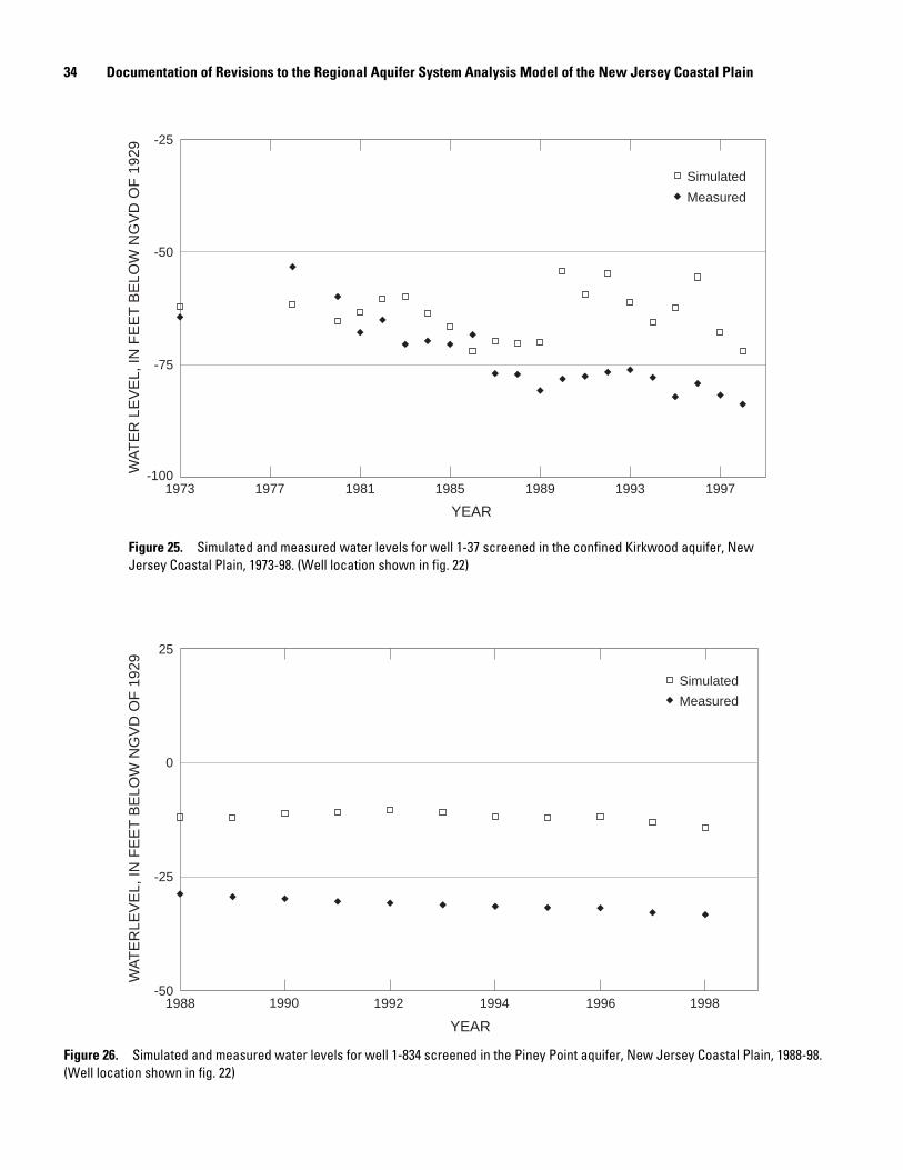
34 Documentation of Revisions to the Regional Aquifer System Analysis Model of the New Jersey Coastal Plain

-100

-75

-50

-25

Measured

Simulated

WA

TE

R L

EV

EL,

IN F

EE

T B

ELO

W N

GV

D O

F 1

929

1973 1977 1981 1985 1989 1993 1997

YEAR

Figure 25. Simulated and measured water levels for well 1-37 screened in the confined Kirkwood aquifer, New Jersey Coastal Plain, 1973-98. (Well location shown in fig. 22)

-50

-25

0

25

Simulated

Measured

WA

TE

RLE

VE

L, IN

FE

ET

BE

LOW

NG

VD

OF

192

9

1988 1990 1992 1994 1996 1998

YEAR

Figure 26. Simulated and measured water levels for well 1-834 screened in the Piney Point aquifer, New Jersey Coastal Plain, 1988-98. (Well location shown in fig. 22)

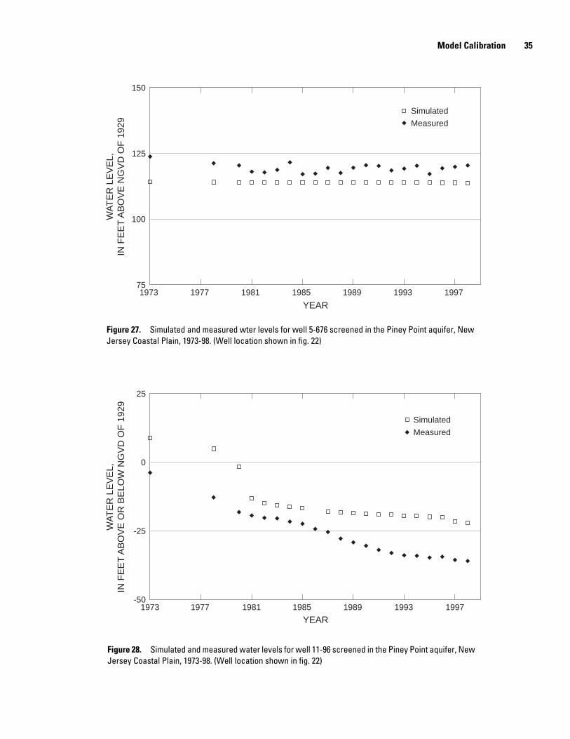
35 Model Calibration

75

100

125

150

Measured

SimulatedW

AT

ER

LE

VE

L,IN

FE

ET

AB

OV

E N

GV

D O

F 1

929

1973 1977 1981 1985 1989 1993 1997

YEAR

Figure 27. Simulated and measured wter levels for well 5-676 screened in the Piney Point aquifer, New Jersey Coastal Plain, 1973-98. (Well location shown in fig. 22)

-50

-25

0

25

Measured

Simulated

WA

TE

R L

EV

EL,

IN F

EE

T A

BO

VE

OR

BE

LOW

NG

VD

OF

192

9

1973 1977 1981 1985 1989 1993 1997

YEAR

Figure 28. Simulated and measured water levels for well 11-96 screened in the Piney Point aquifer, New Jersey Coastal Plain, 1973-98. (Well location shown in fig. 22)

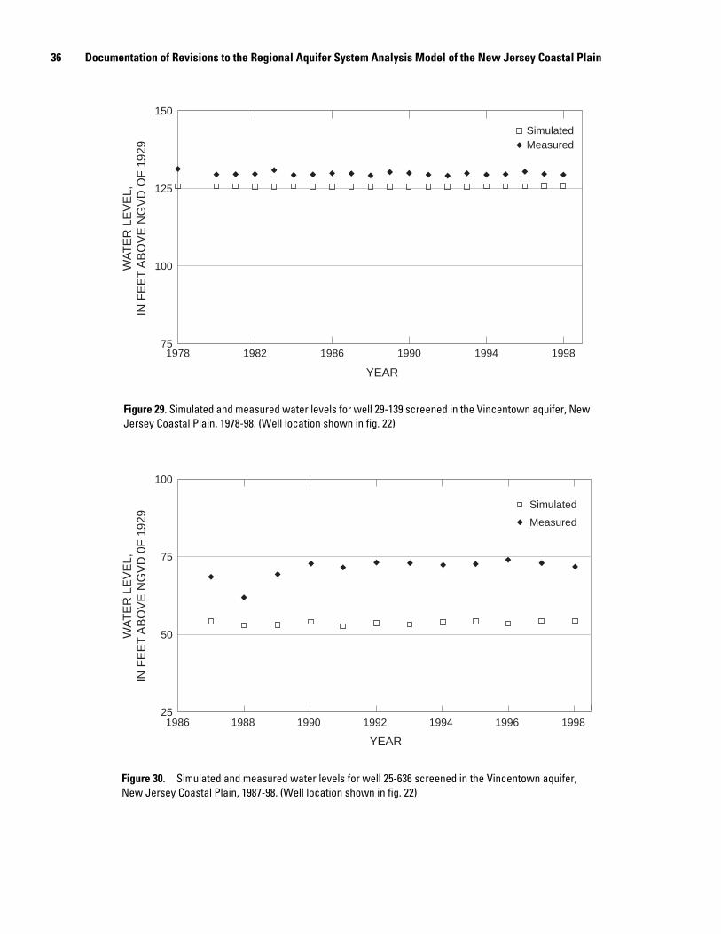
36 Documentation of Revisions to the Regional Aquifer System Analysis Model of the New Jersey Coastal Plain

75

100

125

150

Measured Simulated

WA

TE

R L

EV

EL,

IN F

EE

T A

BO

VE

NG

VD

OF

192

9

1978 1982 1986 1990 1994 1998

YEAR

Figure 29. Simulated and measured water levels for well 29-139 screened in the Vincentown aquifer, New Jersey Coastal Plain, 1978-98. (Well location shown in fig. 22)

25

50

75

100

Measured

Simulated

WA

TE

R L

EV

EL,

IN F

EE

T A

BO

VE

NG

VD

0F

192

9

1986 1988 1990 1992 1994 1996 1998

YEAR

Figure 30. Simulated and measured water levels for well 25-636 screened in the Vincentown aquifer, New Jersey Coastal Plain, 1987-98. (Well location shown in fig. 22)

37 Model Calibration

25 W

AT

ER

LE

VE

L,IN

FE

ET

AB

OV

E O

R B

ELO

W S

EA

LE

VE

L

0

-25 1984 1986 1988 1990 1992 1994 1996 1998

Measured

Simulated

YEAR

Figure 31. Simulated and measured water levels for well 25-353 screened in the Wenonah-Mount Laurel aquifer, New Jersey Coastal Plain, 1984-97.

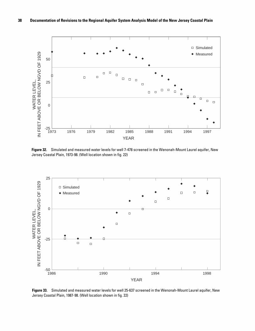
38 Documentation of Revisions to the Regional Aquifer System Analysis Model of the New Jersey Coastal Plain

-25

0

25

50 Measured

Simulated

WA

TE

R L

EV

EL,

IN F

EE

T A

BO

VE

OR

BE

LOW

NG

VD

OF

192

9

1973 1976 1979 1982 1985 1988 1991 1994 1997

YEAR

Figure 32. Simulated and measured water levels for well 7-478 screened in the Wenonah-Mount Laurel aquifer, New Jersey Coastal Plain, 1973-98. (Well location shown in fig. 22)

-50

-25

0

25

Measured

Simulated

WA

TE

R L

EV

EL,

IN F

EE

T A

BO

VE

OR

BE

LOW

NG

VD

OF

192

9

1986 1990 1994 1998

YEAR

Figure 33. Simulated and measured water levels for well 25-637 screened in the Wenonah-Mount Laurel aquifer, New Jersey Coastal Plain, 1987-98. (Well location shown in fig. 22)

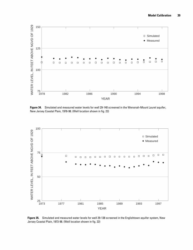
39 Model Calibration

75

100

125

1509

Measured

SimulatedW

AT

ER

LE

VE

L, IN

FE

ET

AB

OV

E N

GV

D O

F 1

92

1978 1982 1986 1990 1994 1998

YEAR

Figure 34. Simulated and measured water levels for well 29-140 screened in the Wenonah-Mount Laurel aquifer, New Jersey Coastal Plain, 1978-98. (Well location shown in fig. 22)

25

50

75

100

Measured

Simulated

WA

TE

R L

EV

EL,

IN F

EE

T A

BO

VE

NG

VD

OF

192

9

1973 1977 1981 1985 1989 1993 1997

YEAR

Figure 35. Simulated and measured water levels for well 29-138 screened in the Englishtown aquifer system, New Jersey Coastal Plain, 1973-98. (Well location shown in fig. 22)

40 Documentation of Revisions to the Regional Aquifer System Analysis Model of the New Jersey Coastal Plain

-175

-150

-125

-100

-75

-50

-25

09

Measured

Simulated

WA

TE

R L

EV

EL,

IN F

EE

T B

ELO

W N

GV

D O

F 1

92

1978 1982 1986 1990 1994 1998

YEAR

Figure 36. Simulated and measured water levels for well 25-429 screened in the Englishtown aquifer system, New Jersey Coastal Plain, 1978-98. (Well location shown in fig. 22)

-75

-50

-25

0

25

50

Measured

Simulated

WA

TE

R L

EV

EL,

IN F

EE

T A

BO

VE

OR

BE

LOW

NG

VD

OF

192

9

1986 1988 1990 1992 1994 1996 1998

YEAR

Figure 37. Simulated and measured water levels for well 25-638 screened in the Englishtown aquifer system, New Jersey Coastal Plain, 1987-98. (Well location shown in fig. 22)

41 Model Calibration

0

25

50

75

Measured

SimulatedW

AT

ER

LE

VE

L, IN

FE

ET

AB

OV

E N

GV

D 1

929

1973 1977 1981 1985 1989 1993 1997

YEAR

Figure 38. Simulated and measured water levels for well 5-259 screened in the Englishtown aqifer system, New Jersey Coastal Plain, 1973-98. (Well location shown in fig. 22)

-75

-50

-25

0

Measured

Simulated

WA

TE

R L

EV

EL,

IN F

EE

T B

ELO

W N

GV

D O

F 1

929

1973 1977 1981 1985 1989 1993 1997

YEAR

Figure 39. Simulated and measured water levels for well 5-258 screened in the Upper Potomac-Raritan-Magothy aquifer, New Jersey Coastal Plain, 1973-98. (Well location shown in fig. 22)

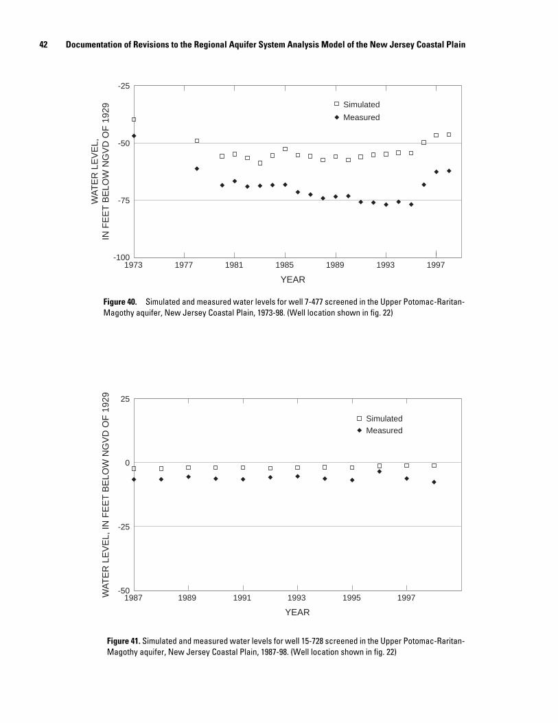
42 Documentation of Revisions to the Regional Aquifer System Analysis Model of the New Jersey Coastal Plain

-100

-75

-50

-25

1973 1977 1981 1985 1989 1993 1997

Measured

Simulated W

AT

ER

LE

VE

L,IN

FE

ET

BE

LOW

NG

VD

OF

192

9

YEAR

Figure 40. Simulated and measured water levels for well 7-477 screened in the Upper Potomac-Raritan-Magothy aquifer, New Jersey Coastal Plain, 1973-98. (Well location shown in fig. 22)

-50

-25

0

25

Measured Simulated

WA

TE

R L

EV

EL,

IN F

EE

T B

ELO

W N

GV

D O

F 1

929

1987 1989 1991 1993 1995 1997

YEAR

Figure 41. Simulated and measured water levels for well 15-728 screened in the Upper Potomac-Raritan-Magothy aquifer, New Jersey Coastal Plain, 1987-98. (Well location shown in fig. 22)

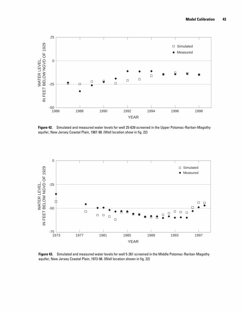
43 Model Calibration

-50

-25

0

25

Measured

Simulated

WA

TE

R L

EV

EL,

IN F

EE

T B

ELO

W N

GV

D O

F 1

929

1986 1988 1990 1992 1994 1996 1998

YEAR

Figure 42. Simulated and measured water levels for well 25-639 screened in the Upper Potomac-Raritan-Magothy aquifer, New Jersey Coastal Plain, 1987-98. (Well location show in fig. 22)

-75

-50

-25

0

Measured

Simulated

WA

TE

R L

EV

EL,

IN F

EE

T B

ELO

W N

GV

D O

F 1

929

1973 1977 1981 1985 1989 1993 1997

YEAR

Figure 43. Simulated and measured water levels for well 5-261 screened in the Middle Potomac-Raritan-Magothy aquifer, New Jersey Coastal Plain, 1973-98. (Well location shown in fig. 22)

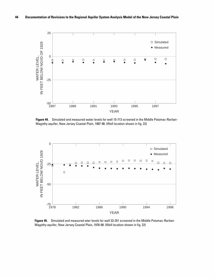
44 Documentation of Revisions to the Regional Aquifer System Analysis Model of the New Jersey Coastal Plain

-50

-25

0

25

Measured

Simulated

WA

TE

R L

EV

EL,

IN F

EE

T B

ELO

W N

GV

D O

F 1

929

Figure 44.

1987 1989 1991 1993 1995 1997

YEAR

Simulated and measured water levels for well 15-713 screened in the Middle Potomac-Raritan-Magothy aquifer, New Jersey Coastal Plain, 1987-98. (Well location shown in fig. 22)

-75

-50

-25

0

Measured

Simulated

WA

TE

R L

EV

EL.

IN F

EE

T B

ELO

W N

GV

D 1

929

Figure 45.

1978 1982 1986 1990 1994 1998

YEAR

Simulated and measured wter levels for well 33-251 screened in the Middle Potomac-Raritan-Magothy aquifer, New Jersey Coastal Plain, 1978-98. (Well location shown in fig. 22)

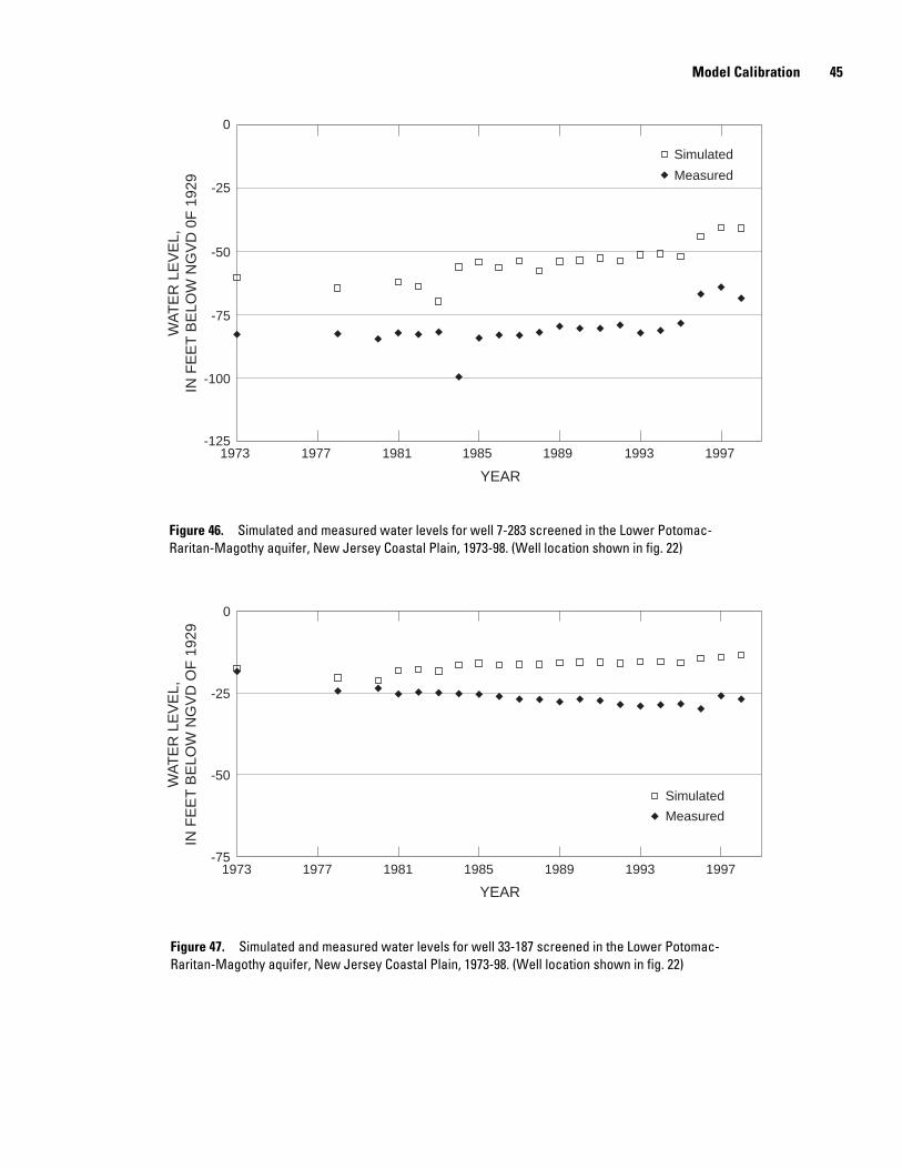
45 Model Calibration

-125

-100

-75

-50

-25

0

Measured

Simulated W

AT

ER

LE

VE

L,IN

FE

ET

BE

LOW

NG

VD

0F

192

9

1973 1977 1981 1985 1989 1993 1997

YEAR

Simulated and measured water levels for well 7-283 screened in the Lower Potomac-Figure 46. Raritan-Magothy aquifer, New Jersey Coastal Plain, 1973-98. (Well location shown in fig. 22)

-75

-50

-25

0

Measured

Simulated

WA

TE

R L

EV

EL,

IN F

EE

T B

ELO

W N

GV

D O

F 1

929

1973 1977 1981 1985 1989 1993 1997

YEAR

Figure 47. Simulated and measured water levels for well 33-187 screened in the Lower Potomac-Raritan-Magothy aquifer, New Jersey Coastal Plain, 1973-98. (Well location shown in fig. 22)

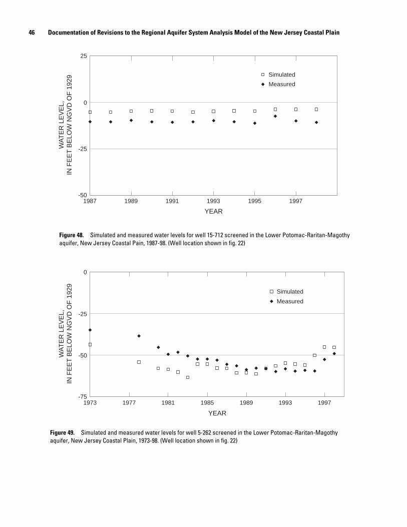
46 Documentation of Revisions to the Regional Aquifer System Analysis Model of the New Jersey Coastal Plain

-50

-25

0

25

Measured

Simulated

WA

TE

R L

EV

EL,

IN F

EE

T B

ELO

W N

GV

D O

F 1

929

1987 1989 1991 1993 1995 1997

YEAR

Figure 48. Simulated and measured water levels for well 15-712 screened in the Lower Potomac-Raritan-Magothy aquifer, New Jersey Coastal Pain, 1987-98. (Well location shown in fig. 22)

-75

-50

-25

0

Measured

Simulated

WA

TE

R L

EV

EL,

IN F

EE

T B

ELO

W N

GV

D O

F 1

929

1973 1977 1981 1985 1989 1993 1997

YEAR

Figure 49. Simulated and measured water levels for well 5-262 screened in the Lower Potomac-Raritan-Magothy aquifer, New Jersey Coastal Plain, 1973-98. (Well location shown in fig. 22)

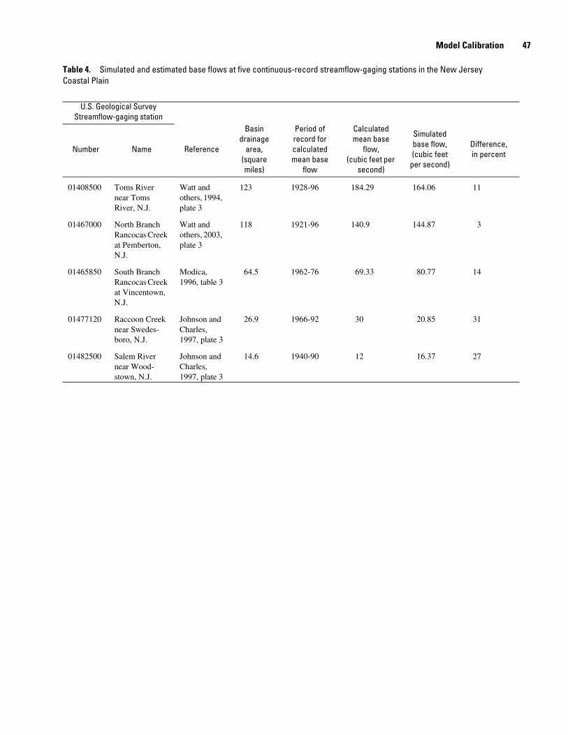
47 Model Calibration

Table 4. Simulated and estimated base flows at five continuous-record streamflow-gaging stations in the New Jersey Coastal Plain

U.S. Geological Survey Streamflow-gaging station

Number Name Reference

Basin drainage

area, (square miles)

Period of record for calculated mean base

flow

Calculated mean base

flow, (cubic feet per

second)

Simulated base flow, (cubic feet

per second)

Difference, in percent

01408500 Toms River Watt and 123 1928-96 184.29 164.06 11 near Toms others, 1994, River, N.J. plate 3

01467000 North Branch Watt and 118 1921-96 140.9 144.87 3 Rancocas Creek others, 2003, at Pemberton, plate 3 N.J.

01465850 South Branch Modica, 64.5 1962-76 69.33 80.77 14 Rancocas Creek 1996, table 3 at Vincentown, N.J.

01477120 Raccoon Creek Johnson and 26.9 1966-92 30 20.85 31 near Swedes- Charles, boro, N.J. 1997, plate 3

01482500 Salem River Johnson and 14.6 1940-90 12 16.37 27 near Wood- Charles, stown, N.J. 1997, plate 3

48 Documentation of Revisions to the Regional Aquifer System Analysis Model of the New Jersey Coastal Plain

Summary

As part of an ongoing program to maintain ground-water-flow models constructed in New Jersey, the U.S. Geological Survey (USGS), in cooperation with New Jersey Department of Environmental Protection (NJDEP), developed a standardized procedure to archive the models and revise selected models by incorporating recent data, such as withdrawal data and simula­tion techniques. The Regional Aquifer System Analysis finite-difference numerical model of flow in the New Jersey Coastal Plain sediments (Martin, 1998) was revised by (1) rediscretiz­ing the model parameters with a finer cell size, (2) using a spa­tially variable recharge rate that is based on rates determined in studies conducted since the model was initially developed in 1981, and (3) using recent ground-water withdrawal data for 1982-98.

The revised New Jersey Coastal Plain model can be used as a tool to evaluate the regional effect on water levels of changes in ground-water withdrawals. The model can aid in re­evaluating water-management strategies in the New Jersey Coastal Plain.

The revised model was calibrated by trail-and-error adjust­ment of the storage coefficient, vertical leakance, streambed conductance, lateral-boundary fluxes, and recharge rates. Recharge rates were adjusted in areas where no previous studies had been done to estimate the spatial variation of recharge rates. These five parameters were adjusted during model calibration in order to minimize the difference between simulated and mea­sured values of one or more of the following: (1) estimated base flow in five river basins, (2) water levels in 28 observation wells for which long-term hydrographs were available, and (3) poten­tiometric surfaces for 1978, 1983, 1988, 1993, and 1998 ground-water-flow conditions.

Water levels in the regional cone of depression centered near the Monmouth and Ocean County boundary in the Wenonah-Mount Laurel aquifer and Englishtown aquifer sys­tem have risen about 100 ft from 1988 to 1998. The rise in water levels in this area is due to a decrease in ground-water with­drawals. Model calibration revealed that storage coefficient is an important parameter in the recovery of water levels in this area. It appears that a large portion of the ground water flowing into this area is going into aquifer storage. Water levels in observation wells screened within the regional cone of depres­sion centered near the Monmouth and Ocean County boundary in the Wenonah-Mount Laurel aquifer and Englishtown aquifer system have been increasing since 1989; therefore, water levels have not reached steady-state conditions with current (1998) ground-water withdrawals.

References Cited

Barton, Cynthia, and Kozinski, Jane, 1991, Hydrogeology of the region of Greenwich Township, Gloucester County, New Jersey: U.S. Geological Survey Water-Resources Investiga­tions Report 90-4198, 77 p.

Charles, E.G., Storck, D.A., and Clawges, R.M., 2001 Hydrol­ogy of the unconfined aquifer system, Maurice River area: Maurice and Cohansey River basins, New Jersey, 1994-95: U.S. Geological Survey Water-Resources Investigations Report 01-4229, 5 sheets.

Harbaugh, A.W., and McDonald, M.G., 1996, User's documen­tation for MODFLOW-96, an update to the U.S. Geological Survey modular finite-difference ground-water flow model: U.S. Geological Survey Open-File Report 96-485, 56 p.

Johnson, M.L., and Charles, E.G., 1997, Hydrogeology of the unconfined aquifer system, Salem River area: Salem River and Raccoon, Oldmans, Alloway, and Stow Creek Basins, New Jersey, 1993-94: U.S. Geological Survey Water-Resources Investigations Report 96-5195, 5 sheets.

Johnson, M.L., and Watt, M.K., 1996, Hydrogeology of the unconfined aquifer system, Mullica River Basin, New Jersey, 1991-92: U.S. Geological Survey Water-Resources Investi­gations Report 94-4234, 6 sheets.

Lacombe, P.J., and Rosman, Robert, 1995, Hydrology of the unconfined aquifer system in the upper Maurice River basin and adjacent areas in Gloucester County, New Jersey, 1986­87: U.S. Geological Survey Water-Resources Investigations Report 92-4128, 5 sheets.

Lacombe, P.J., and Rosman, Robert, 2001, Water levels in, extent of freshwater in, and water withdrawals from ten con­fined aquifers, New Jersey and Delaware Coastal Plain, 1998: U.S. Geological Survey Water-Resources Investiga­tions Report 00-4143, 10 sheets.

Leahy, P.P., 1982, A three-dimensional ground-water-flow model modified to reduce computer-memory requirements and better simulate confining-bed and aquifer pinch outs: U.S. Geological Survey Water-Resources Investigations Report 82-4023, 59 p.

Leahy, P.P., and Martin, Mary, 1993, Geohydrology and simu­lation of ground-water flow in the Northern Atlantic Coastal Plain aquifer system: U.S. Geological Survey Professional Paper 1404-K, 81 p.

Lewis, J.C., Hochreiter, J.J., Barton, G.J., and Kozinski, Jane, 1991, Hydrogeology of, and ground-water quality in, the Potomac-Raritan-Magothy aquifer system in the Logan Township region, Gloucester and Salem Counties, New Jer­sey: U.S. Geological Survey Water-Resources Investigations Report 90-4142, 92 p.

Martin, Mary, 1998, Ground-water flow in the New Jersey Coastal Plain: U.S. Geological Survey Professional Paper 1404-H, 146 p.

McDonald, M.G., and Harbaugh, A.W., 1988, A modular three-dimensional finite-difference ground-water flow model: U.S. Geological Survey Techniques of Water-Resources Investi­gations, book 6, chap. A1, 586 p.

Meisler, Harold, 1980, Preliminary delineation of salty ground water in the northern Atlantic Coastal Plain of New Jersey: U.S. Geological Survey Open-File Report 81-71, 37 p.

Modica, Edward, 1996, Simulated effects of alternative with­drawal strategies on ground-water flow patterns, New Jersey Pinelands: U.S. Geological Survey Water-Resources Investi­gations Report 95-4133, 46 p.

Nicholson, R.S., and Watt, M.K., 1997, Simulation of ground­water flow in the unconfined aquifer system of the Toms River, Metedconk River, and Kettle Creek Basins, New Jer­sey: U.S. Geological Survey Water-Resources Investigations Report 97-4066, 100 p.

Pope, D. A., and Gordon, A. D., 1999, Simulation of ground­water flow and movement of the freshwater-saltwater inter­face in the New Jersey Coastal Plain: U.S. Geological Survey Water-Resources Investigations Report 98-4216, 159 p.

Seaber, P.R., 1965, Variations in chemical character of water in the Englishtown Formation, New Jersey: U.S. Geological Survey Professional Paper 498-B, 35 p.

Sloto, R.A., and Crouse, M.Y., 1996, HYSEP: A computer pro­gram for streamflow-hydrograph separation and analysis: U.S. Geological Survey Water-Resources Investigations Report 96-4040, 46 p.

Spitz, F.J., 1998, Analysis of ground-water flow and saltwater encroachment in the shallow aquifer system of Cape May County, New Jersey: U.S. Geological Survey Water-Supply Paper 2490, 51 p.

Trescott, P.C., 1975, Documentation of finite-difference model for simulation of three-dimensional ground-water flow: U.S. Geological Survey Open-File Report 75-438, 103 p.

Walker, R.L., 1983, Evaluation of water levels in major aquifers of the New Jersey Coastal Plain, 1978: U.S. Geological Survey Water-Resources Investigations Report 82-4077, 56 p.

Watt, M.K., 2000, A hydrologic primer for New Jersey water­shed management: U.S. Geological Survey Water-Resources Investigations Report 00-4140, 108 p.

Watt, M.K., and Johnson, M.L., 1992, Water resources of the unconfined aquifer system of the Great Egg Harbor River basin, New Jersey, 1989-90: U.S. Geological Survey Water-Resources Investigations Report 91-4126, 5 pls.

Watt, M.K., Johnson, M.L., and Lacombe, P.J., 1994, Hydrol­ogy of the unconfined aquifer system, Toms River, Metede­conk River, and Kettle Creek Basins, New Jersey, 1987-90: U.S. Geological Survey Water-Resources Investigations Report 93-4110, 5 sheets.

References Cited 49

Watt, M.K., Kane, A.C., Charles, E.G., and Storck, D.A., 2003, Hydrology of the unconfined aquifer system, Rancocas Creek area: Rancocas, Crosswicks, Assunpink, Blacks, and Crafts Creek Basins, New Jersey, 1996: U.S. Geological Survey Water-Resources Investigations Report 02-4280, 5 sheets.

Zapecza, O.S., 1989, Hydrogeologic framework of the New Jersey Coastal Plain: U.S. Geological Survey Professional Paper 1404-B, 49 p., 24 pl.

Voronin, Lois M.—

Documentation of Revisions to the Regional A

quifer System A

nalysis Model of the N

ew Jersey Coastal Plain—

U

.S. Geological Survey Water-Resources Investigations 03-4268

Printed on recycled paper