Water quality model for non point source pollutants

*Corresponding author.

1944-3994 / 1944-3986 © 2019 Desalination Publications. All rights reserved.

Desalination and Water Treatmentwww.deswater.com

doi:10.5004/dwt.2019.24684

164 (2019) 111–120October

Water quality model for non point source pollutants incorporating bioretention with EPA SWMM

Sezar GülbazIstanbul University-Cerrahpaşa, Department of Civil Engineering, Avcılar, 34320, Istanbul, Turkey, Tel. +90-212-473-70-00/17941, Fax +90-212-473-71-80, email: [email protected] (S. Gülbaz)

Received 8 January 2019; Accepted 8 July 2019

a b s t r a c t

The first aim of this study is to develop a calibrated water quality model of the non-point source pol-lutants over the experimental drainage area. And, the second aim is to incorporate the bioretention into the water quality model to observe its performance on pollutant removal. The study makes use of the Environmental Protection Agency Storm Water Management Model (EPA SWMM) which is being described in literature as a reliable software tool, and of the Rain fall-Watershed-Bioretention (RWB) System which is a previously developed experimental system that consists of an artificial rainfall system, drainage area and bioretention column. Within this scope, zinc (Zn), copper (Cu), lead (Pb), total nitrogen (TN) and total phosphate (TP) are defined as pollutants in the model. Bio-retention is then integrated into the model, and all values related to bioretention are entered in the program. Hydrographs and pollutographs, showing the effects of non-point source pollution sources at the outlet of the drainage area, are obtained from the model before and after bioretention imple-mentation. The values measured at the outlets of the drainage area and bioretention are compared with the results obtained from the model, and the model is calibrated accordingly. Based on the cal-ibration results, the pollutant build-up and pollutant wash-off coefficients are obtained for the water quality model. Moreover, the effect and performance of bioretention on the quality of surface runoff are examined by evaluating the results of the model and the experiment. It is observed that the reductions of peak flow and of water contamination are very high after bioretention. Moreover, it is concluded that although the non-point source pollution model performance of EPA SWMM without bioretention is successful in representing peak concentration and the shape of the pollutographs, the model performance with bioretention needs further improvement.

Keywords: Pollutant build-up; Pollutant wash-off; Water quality model; Bioretention; EPA SWMM; Storm water treatment

1. Introduction

Investigating sources of pollution is of critical impor-tance in ensuring protection of water resources, and environ-mental sustainability. While sources of pollution generally differ among water basins, there are still certain pollutants that are common for all the water basins [1]. Pollutants, that affect water resources, are categorized as either point source or non-point source pollutants. Non-point source pollutants are ones that do not have a single source, and that have dif-fused. This type of pollution is caused by the gradual sur-

face build-up of small quantities of certain pollutants. One of the most known examples of this is the pollution result-ing from the nutrient (TN and TP) build-up in time due to the use of fertilizers on farmlands [2,3]. Another example of non-point source pollutants is heavy metals such as Zn, Cu and Pb that accumulate in time at parking areas. The accumulating pollution is calculated by the build-up func-tion [4]. These pollutants, that build-up on the surface, are then washed off by rain, and blended with surface runoff. The transport of pollutants, that mix with surface runoff, is calculated by the wash-off function [5]. Moreover, there are various parameters affecting non-point source pollu-tion such as physical and chemical properties, and amounts

S. Gülbaz / Desalination and Water Treatment 164 (2019) 111–120112

of pollutants, land use and soil types [6,7], basin slope [8], vegetation of the catchment [9], rainfall intensity and dura-tion [10], and antecedent dry days [11] to define and model the non-point source. Analyzing and modeling non-point source pollution runoff characteristics are difficult, because the pollutants are generated and diffused ubiquitously [12]. Literature contains a number of field studies showing the surface distribution of non-point source pollutants [13–15], however there is only a limited number of modeling stud-ies analyzing the variation of non-point source pollutants in surface runoff in time. For this reason, there is need for modeling studies that will be able to predict the behaviors of non-point source pollutants in surface runoff [16,17].

Various methods are required to be implemented to pre-vent non-point source pollutants, and to limit the effect of first flush which is the first, faster and more contaminated runoff [18]. For this purpose, low impact development (LID) implementations have recently been recognized as a useful solution [19–22] to eliminate or reduce non-point source pollution in order to meet water quality criteria without disturbing environmental quality [23]. Some LID types are green roof, bioretention, storm water wetland, rain barrel, vegetative swale and permeable asphalt and pavement [24]. Bioretention is one of the most frequently used LID implementation [25] to decrease peak flow, and to increase water quality. Literature covers a number of stud-ies indicating that bioretention is reducing the peak flow of surface runoff, increasing evapotranspiration and infiltra-tion, and reducing pollution in water sources. Bioretention plays an important role in the treatment of the heavy metals and nutrients that mix with storm water, and that pose a significant threat to water resources [26]. There are vari-ous studies, that involved the measurement of Cu, Pb and Zn in the field, in literature investigating the performance and effect of bioretention on heavy metal treatment [27,28]. Glass and Bissouma [29] reported that treatment at a ratio of 81% occurred in Cu, at a rate of 79% in Zn, and at a rate of 75% in Pb is achieved by implementing bioretention at the exit of a parking area. In a bioretention study, Hatt et al. [30] identified treatment ratio of 90% for copper, lead and zinc. Moreover, a study conducted in Australia showed that bioretention is effective in the treatment of Nitrogen (TN) at a ratio of 70%, and of phosphorus (TP) at a ratio of 70% [31].

In recent years, the modeling of non-point sources in storm water runoff and in LID implementations such as bioretention turned out to be a complex task and an increas-ingly important environmental issue for urban communities. There are some reliable computer models for simulating and predicting the quality of urban storm water in order to deal with this issue. EPA SWMM software is a reliable program for modeling the diffusion of non-point source pollution, and for the formation of hydrologic, hydraulic, water quality models and LID models [32]. Literature contains many studies that use the EPA SWMM to produce and calibrate hydrologic and hydraulic models of surface runoff resulting from rainfall [33,34], but there are rare studies modeling and calibrating the behaviors of non-point source pollutants in surface run-off within the scope of water quality modeling efforts. Hence, there is need for well-calibrated water quality models. Also, LID implementations performed by using the EPA SWMM program are very recent and the number of studies on this issue is quite limited in literature [35,36].

The objectives of this study are (1) to produce a cali-brated water quality model of the non-point source pollut-ants on the experimental drainage area, (2) to incorporate the bioretention into the water quality model to observe its performance on pollutant removal. For this purpose, the drainage area, artificial rain intensity system and bioreten-tion column in the RWB system, five pollutants such as Zn, Cu, Pb, TN and TP, and EPA SWMM consisting the build-up and wash-off functions and the coefficients of these func-tions are used in the model. Hydro graphs and polluto-graphs, showing non-point source pollutants, are obtained from the model regarding the conditions before and after the bioretention implementation. The values measured at the outlets of the drainage area and bioretention are com-pared with the results obtained from the model, and the model is calibrated accordingly. In this context, a calibrated model is developed to determine the drainage area water quality resulting in non-point source pollutants.

2. Material and methods

2.1. EPA SWMM

EPA SWMM is a computer program that creates dynamic simulations of the surface runoff formed by storm water, and it can model the quantity and quality of water in the surface runoff resulting from discrete (for example, one day long) and continuous (for example, one year long) precipitations [37,38]. As a program, EPA SWMM can calculate the quantity and quality of surface runoff that forms in each sub-catch-ment area within a basin system, as well as the flow rate, depth and pollutant concentration that forms in each pipe and channel. Inputs provided to the EPA SWMM program include the hyetograph (the change in precipitation inten-sity in time) and information that characterizes the basin, such as the length of the basin, flow direction in the basin, the impervious area in the basin, and the length, width and cross-section of the pipes and channels. The outputs from the program include a hydrograph (changes in flow in time) and a pollutograph (change in concentrations in time).

2.1.1. Hydrology and hydraulics modules of SWMM

EPA SWMM solves the continuity and momentum equa-tions using finite difference method in order to calculate the flow rate. Kinematic, diffusion, and dynamic wave methods are the routing options in EPA SWMM. The dynamic wave method is the most general form of the flood routing equa-tions which represents unsteady and non-uniform flow. Diffusion wave equations are obtained by neglecting the inertial term, and kinematic wave equations are obtained by neglecting both the inertial and pressure terms in the momentum equation of the dynamic wave method. EPA SWMM calculates infiltration using five different methods, namely Green-Ampt, Horton, Modified Green-Ampt, Mod-ified Horton, and Curve Number (CN) Method. Moreover, there is LID control editor in EPA SWMM under hydrology module. It is capable of simulating the LID performance, including bioretention, rain gardens, green roofs, infiltra-tion trenches, permeable pavements, rain barrels, and veg-etative swales. There are various layers such as surface,

S. Gülbaz / Desalination and Water Treatment 164 (2019) 111–120 113

pavement, soil, storage and drain layer. These layers are used based on the type of LID selected.

2.1.2 Water quality module of SWMM

EPA SWMM calculates water quality routing in the drainage network assuming that the conduits behave as a continuous-flow stirred-tank reactor (CSTR). Pollutant build-up functions in EPA SWMM are exponential, power and saturation functions. Moreover, pollutant wash-off functions are exponential, rating curve and event mean concentration functions. In this study, exponential build-up and wash-off functions are used as follows [38]:

( )21 1 C tB C e−= − (1)

43

CBw C q m= (2)

where B is the mass of buildup per unit area (M/L2), mB is the mass of buildup (M), C1 is the possible maximum build-up on sub-catchment surface (M/L2), C2 is the build-up rate con-stant (1/T), and t is the time (T), w is the amount of wash-off pollutant (M/T), C3 is the pollutant wash-off coefficient ((L/T)–C4 T–1), C4 is the wash-off exponent (dimensionless), and q is the runoff rate over the sub-catchment (L/T).

2.2. Experimental setup - RWB system

The RWB system is constructed on a 150 m2 area adja-cent to the Civil Engineering Department of the Istanbul

University-Cerrahpaşa Avcılar Campus [39]. Photo and schematic of RWB experimental system are shown in Fig. 1. This area is comprised of an artificial rainfall system consisting of 40 nozzle sprinkler, a 40 m2 drainage area, and a bioretention column. In the system, 40 m2 of imper-meable-surfaced galvanized sheet metals are used to rep-resent the drainage area. The drainage area in the RWB system has 2 m long, 4 m wide, and slope of 0.7%. In gen-eral, 3–5% of the LID area of the catchment is used for the LID model. Therefore, in this study, 8 m2 of the RWB sys-tem is used for surface runoff generation since the bioret-ention surface area is 0.23 m2, which corresponds to 2.9% of the drainage area.

In order to apply artificial precipitation to the drainage area, a steel structure containing 40 nozzles, aligned in 10 rows at a height of 1 meter, is established above the drain-age area. The artificial precipitation system also contains a 5 m3 water tank, one pump, one flow meter, 12 valves and a number of pipes.

A single bioretention column is used in the study. In accordance with the design criteria for bioretention media [40,41], the column contains 40 kg of gravel at the bottom, 230 kg of a mixture of sand and vegetative soil in the mid-dle, and 3.5 kg of mulch at the top. Particle sizes and tex-tures of sand and vegetative soil are determined to meet the design criteria for bioretention media. And, dry bulk den-sity, specific gravity of solid, void ratio, porosity, organic matter ratio, and initial moisture content for bioretention column are measured and calculated as 1.43 g/mL, 2.6, 0.82, 0.45, 2.31%, and 18% respectively. Furthermore, the berm height (storage depth), the thickness of the soil layer, stor-age thickness and the conductivity of the bioretention col-

Fig. 1. Photo and schematic of Rainfall-Watershed-Bioretention (RWB) system.


umn are measured as 410 mm, 680 mm, 100 mm and 380 mm/h, respectively. The bioretention column has a height of 124 cm, a diameter of 54 cm, a surface area of 0.23 m2 and surface slope of 0%. A polyvinyl chloride (PVC) pipe is used to transfer the water collected in the drainage area to the bioretention column.

2.3. Sampling and measurement

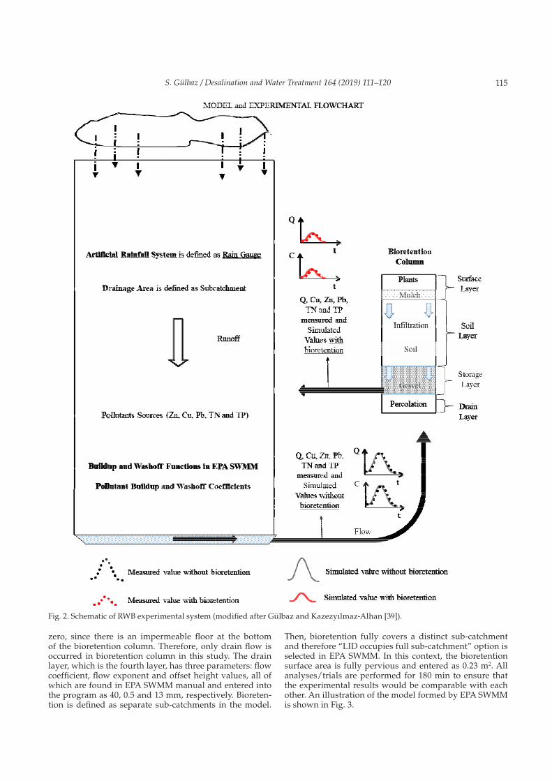
RWB setup is used to investigate water quality per-formance of bioretention in storm water treatment. Accu-mulation of pollutants takes a long time to build-up pollutants (mostly in days) on a drainage area. In order to control this accumulation and shorten to the accumula-tion time, artificial pollutants are added on the drainage area. Therefore, the performance of bioretention on water quality is evaluated by splashing artificial pollutants which are Zn, Cu, Pb, TN and TP on the drainage area in RWB system. The artificial pollutants spread on drain-age area are lead chloride (PbCl2), zinc chloride (ZnCl2) and copper chloride dehydrates (CuCl2 × 2H2O). 42 g of zinc chloride (ZnCl2) for 20 g Zn, 27 g of lead chloride (PbCl2) for 20 g Pb, and 54 g of copper chloride dehy-drates (CuCl2 × 2H2O) for 20 g Cu are used in this study to provide artificial heavy metal pollutants. Moreover, 1-L liquid and animal manure mixture are used to pro-vide the pollutants resulting from the nutrient (TN and TP). Pollutants added on the drainage area are washed off with surface runoff and reached the bioretention column under the synthetic rainfall. Surface runoff is generated on the RWB system under an artificial rainfall event by using the artificial rainfall system in RWB. Before starting the experiment, the rainfall intensity is adjusted by using the pump, which is part of the artificial rainfall system of the RWB. The rainfall intensity is adjusted and mea-sured 27.5 mm/h on the drainage area. Then, storm water runoff has developed over the drainage area after rain-fall started. Moreover, the rainfall duration is selected as 30 min. Ultimately, the rainfall intensity values are lim-ited based on the manual adjustment of a valve and the measure allows for a reading up to half a millimeter of precipitation depth. The rainfall duration is selected as 30 min since the maximum flow values are reached during this period. After rainfall starts, bioretention inflow and outflow rate are measured at the inlet and outlet of the column for 180 min. In addition to the flow rates, samples are collected at different times from the inlet and outlet of the bioretention column [42]. Then, these samples are ana-lyzed and the inlet and outlet pollutographs are obtained. The model and experimental flowchart are given in Fig. 2.

2.4. Model development with EPA SWMM

The hydrologic-hydraulic and water quality model of the drainage area in which the bioretention would be estab-lished is prepared using the EPA SWMM program. During the modeling stage, the hydrologic and hydraulic parts of the model are developed firstly. For this purpose, sub-catch-ments within the drainage area are defined primarily in the program. The drainage area, width and slope are defined as 8 m2, 4 m, and 0.7%, respectively. Manning’s roughness

coefficient for the impervious area and depth of depres-sion storage on the impervious area are obtained from EPA SWMM manual as 0.015 and 1.27 mm, respectively [38]. These values are also entered in the program. Since the drainage area is a fully impermeable surface, it is defined as a “100% impermeable surface” in the model. And this eliminates the need for the infiltration equations normally used in a drainage area model.

The type of rainfall data is selected as intensity with a value of 27.5 mm/h and the rainfall time interval of the rainfall gauge is selected as one minute in the EPA SWMM model. In addition, the rainfall duration value in the pro-gram is selected as 30 min. Antecedent dry days value is the number of days with no rainfall prior to the start of the simulation and is used to compute pollutant accumulation in EPA SWMM model before the rain starts. After the begin-ning of rainfall, pollutants are washed off and the polluto-graphs are obtained. The maximum initial buildup value is obtained when the antecedent dry days value is selected about 20 d in the model presented in this study. Conse-quently, the simulation of the model starts 20 d before the rainfall. The simulation results in this study are presented beginning of the rainfall in order to be able to show the washoff concentration distribution in time which covers a time period of three hours which is the time period for the experiments.

For the second part of the model, in order to estab-lish the water quality model in EPA SWMM, exponential build-up and exponential wash-off functions are defined for pollutant build-up and pollutant wash-off, respectively. Five pollutant parameters such as Zn, Cu, Pb, TN and TP are defined in the program. Then, water quality input parameters, which belong to the build-up and wash-off functions, are defined in the program. These are the pos-sible maximum build-up on subcatchment surface (C1), the build-up rate constant (C2), the wash-off coefficient (C3), and the wash-off exponent (C4). These parameters are calibrated by using the data measured in the experimental area, and the results are given in the results section.

As the final part, bioretention is integrated into water quality model. In order to define bioretention to the SWMM, parameters of the four layers are required to be entered in the program. The surface layer, which is the first one, has four parameters. The berm height (storage depth) is measured, and entered in the program as 410 mm. Values of vegetation volume, surface roughness (Manning’s N [38]), and surface slope are entered in the program as 0.2 (fraction), 0.13 and 0%, respectively. The soil layer, as the second layer, has seven parameters. The thickness of the soil layer and the conductivity of the soil are both measured and entered in the program as 680 mm and 380 mm/h, respectively. Porosity, field capacity, wilt-ing point, conductivity slope and suction head values are also obtained from EPA SWMM manual [38], and entered into the program as 0.42 (volume fraction), 0.15 (volume fraction), 0.07 (volume fraction), 10 and 19 mm, respec-tively. The storage layer, which is the third layer, has four parameters. The thickness is measured, and entered in the program as 100 mm. Void ratio, seepage rate, and clog-ging factor values are obtained from EPA SWMM manual [38], and entered into the program as 0.75 (voids/solids), 0 and 0, respectively. In this study, seepage rate is selected


zero, since there is an impermeable floor at the bottom of the bioretention column. Therefore, only drain flow is occurred in bioretention column in this study. The drain layer, which is the fourth layer, has three parameters: flow coefficient, flow exponent and offset height values, all of which are found in EPA SWMM manual and entered into the program as 40, 0.5 and 13 mm, respectively. Bioreten-tion is defined as separate sub-catchments in the model.

Then, bioretention fully covers a distinct sub-catchment and therefore “LID occupies full sub-catchment” option is selected in EPA SWMM. In this context, the bioretention surface area is fully pervious and entered as 0.23 m2. All analyses/trials are performed for 180 min to ensure that the experimental results would be comparable with each other. An illustration of the model formed by EPA SWMM is shown in Fig. 3.

Fig. 2. Schematic of RWB experimental system (modified after Gülbaz and Kazezyılmaz-Alhan [39]).


Fig. 3. EPA SWMM model of RWB system.


3. Results and discussion

The flow rate at the outlet of the RWB system is simu-lated by using EPA SWMM with and without bioretention. The measured flow rate at the outlet of the RWB system is obtained both with and without bioretention for the rain-fall event with an intensity of 27.5 mm/h and duration of 30 min. The comparison of the measured and simulated flow rates with and without bioretention is shown in Fig. 4. In this figure, the simulated and measured peak flow rates without bioretention are 3662.10 mL/min, and 3750.00 mL/min, respectively. As seen in the figure, the characteristics of simulated and measured shape of the hydro graphs for without bioretention are very similar. Moreover, the peak values of the simulated and measured hydro graphs with bioretention are 1455.96 mL/min, and 1720.00 mL/min, respectively. As shown by this figure, the results of simu-lated hydro graph with bioretention match well with the experimental results. The percentage of peak flow reduction after bioretention implementation is 60.24% for simulation model, and 54.13% for measured model, and this shows that the calculated reduction percentage of EPA SWMM model is compatible with experimental results.

In order to assess the accuracy of the water quality model, statistical analyses are performed by calculating coefficients of determination for simulated and measured hydro graphs for the case of without bioretention. The coefficient of determination is defined as the square of the Pearson product moment correlation coefficient, R [43]. Coefficient of determination for simulated and measured peak flow rate values without bioretention is calculated as 0.80, and this states that hydro graph of simulated flow is in good agreement with the measured data. In addition, absolute peak errors for the peak values of the hydro graphs are also calculated since peak values are important for first flush runoff. The absolute percentage error for sim-ulated and measured peak flow rate without bioretention is 2.34%. These results show that the hydrological model is successful in representing peak flows of the measured data.

The water quality analyses for non-point source pollu-tion with and without bioretention are simulated by using EPA SWMM for the same rainfall intensity and duration. The measured and simulated concentrations of TN, TP, Pb, Cu, and Zn with and without bioretention are shown in Figs. 5–9. As seen in these figures, the shape of the pol-

lutographs obtained from the simulation results and RWB measurements for the case of without bioretention are very similar except for TP. It is observed that EPA SWMM pro-gram does not model TP pollutants as well as other param-eters. The coefficients of determination for simulated and measured peak concentration in pollutographs for without bioretention are given in Table 3. As seen in this table, coef-ficients of determination values for Pb, TN, Cu, Zn, and TP are calculated as 0.99, 0.97, 0.84, 0.84, and 0.51, respectively. These general results show that non-point source pollution

Fig. 4. Measured and simulated hydro graphs with and without bioretention.

Fig. 5. Measured and simulated total nitrogen (TN) concentra-tion with and without bioretention.

Fig. 6. Measured and simulated total phosphorus (TP) concen-tration with and without bioretention.

Fig. 7. Measured and simulated Lead (Pb) concentration with and without bioretention.


model without bioretention by using EPA SWMM is suc-cessful in representing the water quality behavior of RWB system. However, during simulation with bioretention, it is noticed that EPA SWMM is inadequate in simulating the concentrations of TN, TP, Pb, Cu, and Zn with bioretention implementation. Figs. 5–9 show that although the simulated pollutographs with bioretention by using EPA SWMM has a tendency to approach to the experimental results, there is still room for further improvement for with bioretention case. It means that water quality model with bioretention by using EPA SWMM is required to develop.

The simulated and measured peak concentration with and without bioretention are also given in Table 2. The table shows that the peak concentrations of the simulated and mea-

sured values for the case of without bioretention are close to each other. The absolute percentage error for simulated and measured peak concentration in pollutographs for the case of without bioretention is smaller than 1% as shown in Table 3. Therefore, it is concluded that EPA SWMM can be a practical tool in estimation of peak concentrations for both nutrients and heavy metals in case of no bioretention. In addition, EPA SWMM is also capable of modeling pollutant removal per-formance of bioretentions, however there is room for further improvement in simulating the shape of pollutographs after bioretention involvement in EPA SWMM.

The coefficients of model build-up and wash-off func-tions are investigated to determine parameters which are the possible maximum build-up on sub-catchment surface (C1), the build-up rate constant (C2), the wash-off coefficient (C3), and the wash-off exponent (C4). These coefficients are calibrated by using the experimental results, and they are given in Table 1. Substantially, the build-up and wash-off parameters vary significantly as per location, land use type, basin slope, soil types, vegetation of the catchment, rain-fall intensity and duration, and antecedent dry days, and physical and chemical properties and amounts of pollut-ants. Therefore, coefficients of model build-up and wash-off functions should be investigated by considering aforemen-tioned different variables.

The reduction of different pollutants in bioretention is calculated by using the data obtained before and after bioretention implementation. The reduction values are obtained separately for simulation and experimental results which are summarized in Table 2. As seen from the table, the peak heavy metal concentrations of the simulated and mea-sured data without bioretention are close to each other and the peak heavy metal concentrations with bioretention at the exit are close to zero. The table shows that the reduction of each type of heavy metal in bioretention column is very high for experimental and model results. Therefore, it is observed that bioretention which is natural and commercially avail-able method is very successful solution to prevent heavy metal pollution in storm water. The reduction percentage obtained by simulation results for pollutants of Pb, Cu and Zn after bioretention implementation is much the same with the reduction percentage obtained by experimental results. Furthermore, total nitrogen reduction is 87.63%, and total phosphorus reduction is 70.30% for the experimental results. The simulation reduction results are approximately 99%. It means that although the results of calculation of reduc-tion percentage for simulation results have a tendency to approach to the experimental results, there is still room for further improvement for with bioretention case.

Fig. 8. Measured and simulated copper (Cu) concentration with and without bioretention.

Fig. 9. Measured and simulated zinc (Zn) concentration with and without bioretention.

Table 1 Pollutant build-up and wash-off constant used in EPA SWMM for different pollutants

Maximum build-up C1 (kg/ha)

Build-up rate constant C2 (1/days)

Wash-off coefficient C3 (mm/h)–C4(h)–1

Wash-off exponent C4 (dimensionless)

TN 9.01 0.25 7.00 0.22

TP 2.29 0.40 8.00 0.20

Pb 1.73 0.20 9.00 0.40

Cu 1.28 0.10 4.00 0.40

Zn 12.44 0.30 2.00 0.60


4. Conclusions

In this paper, a simulation model for non-point source pollution of RWB system is generated by using EPA SWMM that is one of the few programs which allows for definition of LID including bioretentions in water quality models. The water quality models are prepared for heavy metals such as Cu, Pb, and Zn, and for nutrients such as TN and TP. The capacity of EPA SWMM in water quality modeling of non-point source pollution and bioretention implementation is also investigated by comparing the model results with the measured data obtained from the RWB system. Moreover, the reduction capacities of bioretention on Cu, Pb, Zn, TN and TP are investigated by using model and experimental results. Finally, the following conclusions are obtained in this study;

(i) Non-point source pollution model by using EPA SWMM without bioretention is successful in repre-senting peak concentration of the measured data in pollutographs. Moreover, the shape of the polluto-graphs obtained from the simulation results and RWB measurements for the case of without bioretention are in good agreement except for TP. However, the con-centration values obtained from the model with bio-

retention implementation by using EPA SWMM does not give similar results to the actual measured values. In light of this observation, it can be said that further development is required for the water quality models for bioretention implementation.

(ii) Based on the calibration results, the pollutant build-up and pollutant wash-off coefficients are obtained for the water quality model. The obtained coefficients and measured values will be useful for future studies to develop new water quality model.

(iii) The reduction of peak flow and of concentration obtained from EPA SWMM model is similar to the experimental results. It is observed that the reduc-tions of peak flow and of water contamination are very high after bioretention implementation. There-fore, it is concluded that bioretention is an economi-cally affordable and commercially available solution to prevent flood and water contamination because of its high reduction performance.

Acknowledgments

This work is supported by Scientific Research Projects Coordination Unit of Istanbul University, Project number BEK-2017-26748. The writer would like to thank Scien-tific Research Projects Coordination Unit of Istanbul Uni-versity.

References

[1] T.C. Winter, J.W. Harvey, O.L. Franke, W.M. Alley, Ground water and surface water: A Single Resource, United States Geological Survey (USGS). Denver, CO. USGS Circular 1998, 1139.

[2] D.D. Poudel, Surface water quality monitoring of an agricul-tural watershed for non point source pollution control, J. Soil Water Conserv., 71 (2016) 310–326.

[3] D.D. Poudel, T. Lee, R. Srinivasan, K. Abbaspour, C.Y. Jeong, Assessment of seasonal and spatial variation of surface water quality, identification of factors associated with water quality variability, and the modeling of critical non point source pollu-tion areas in an agricultural watershed, J. Soil Water Conserv., 68 (2013) 155–171.

Table 2 Simulated and measured peak values and reduction percentage for different pollutants and flow rates with and without bioretention

Simulated peak value without bioretention

Measured peak value without bioretention

Simulated peak value with bioretention

Measured peak value with bioretention

Reduction for simulated peak value with bioretention (%)

Reduction for measured peak value with bioretention (%)

Q flow rate (mL/min) 3662.10 3750.00 1455.96 1720.00 60.24 54.13

TN concentration (mg/L) 380.30 380.00 5.81 47.00 98.47 87.63

TP concentration (mg/L) 100.99 101.00 1.10 30.00 98.91 70.30

Pb concentration (mg/L) 110.45 110.39 0.00 0.00 100.00 100.00

Cu concentration (mg/L) 54.60 54.64 0.71 0.01 98.70 99.99

Zn concentration (mg/L) 536.05 536.30 8.11 0.13 98.49 99.97

Table 3 Values of absolute% errors and coefficient of determination (R2) between experimental data and model results without bioretention

Absolute% error for simulated and measured peak values without bioretention (%)

Coefficient of determination for simulated and measured peak values without bioretention (R2)

Q flow rate 2.34 0.80

TN concentration 0.08 0.97

TP concentration 0.01 0.51

Pb concentration 0.01 0.99

Cu concentration 0.07 0.84

Zn concentration 0.05 0.84


[4] J. Temprano, O. Arango, J. Cagiao, J. Suarez, I. Tejero, Storm-water quality calibration by SWMM: A case study in Northern Spain, Water SA, 32 (2005) 55–63.

[5] T.K. Jewell, D. Adrian, SWMM storm water pollutant wash off functions, J. Environ. Eng. Division, 104 (1978) 1036–1040.

[6] L. Wu, X. Liu, X.Y. Ma, Spatio-temporal variation of ero-sion-type non-point source pollution in a small watershed of hilly and gully region, Chinese Loess Plateau, Environ. Sci. Pollut. Res., 23 (2016) 10957–10967.

[7] Z.Y. Shen, L. Chen, Q. Hong, J.L. Qiu, H. Xie, R.M. Liu, Assess-ment of nitrogen and phosphorus loads and causal factors from different land use and soil types in the Three Gorges Reservoir Area, Sci. Total Environ., 454 (2013) 383–392.

[8] A. Wang, L. Tang, D. Yang, Spatial and temporal variability of nitrogen load from catchment and retention along a river network: a case study in the upper Xin’anjiang catchment of China, Hydrol. Res., 47 (2016) 869–887.

[9] M.A. Lenzi, M. Di Luzio, Surface runoff, soil erosion and water quality modelling in the Alpone watershed using AGNPS inte-grated with a Geographic Information System, Eur. J. Agron., 6 (1997) 1–14.

[10] P. Egodawatta, E. Thomas, A. Goonetilleke, Mathematical interpretation of pollutant wash-off from urban road surface using simulated rainfall, Water Res., 41 (2007) 3025–3031.

[11] H. Hu, G. Huang, Monitoring of non-point source pollutions from an agriculture watershed in South China, Water, 6 (2014) 3828–3840.

[12] S.C. Lee, I.H. Park, B.S. Kım, S.R. Ha, Relationship between non-point source pollution and Korean green factor, Terr. Atmos. Ocean. Sci., 26 (2015) 341–350.

[13] Z. Akdoğan, A. Küçükdoğan, B. Güven, Nonpoint source pol-lutant transport in watersheds: modelling approaches for anti-biotics, heavy metals and nutrients, Int. J. Adv. Eng. Pure Sci., 27 (2015) 21–31.

[14] X.P. Gao, G.N. Li, G.R. Li, C. Zhang, Modeling the effects of point and non-point source pollution on a diversion channel from Yellow River to an artificial lake in China, Water Sci. Technol., 71 (2015) 1806–1814.

[15] Z. Shen, J. Qiu, Q. Hong, L. Chen, Simulation of spatial and temporal distributions of non-point source pollution load in the Three Gorges Reservoir Region, Sci. Total Environ., 493 (2014) 138–146.

[16] Y. Zhuang, T. Nguyen, B. Niu, W. Shao, S. Hong, Research trends in non point source during 1975–2010, International Conference on Medical Physics and Biomedical Engineering (ICMPBE2012), D. Yang, ed., Physics Procedia, 33 (2012) 138–143.

[17] L. Wu, T. Long, X. Liu, J.S. Guo, Impacts of climate and land-use changes on the migration of non-point source nitrogen and phosphorus during rainfall-runoff in the Jialing River Watershed, China, J. Hydrol., 475 (2012) 26–41.

[18] M. Di Modugno, A. Gioia, A. Gorgoglione, V. Iacobellis, G. la Forgia, A.F. Piccinni, E. Ranieri, Build-up/wash-off monitor-ing and assessment for sustainable management of first flush in an urban area, Sustainability, 7 (2015) 5050–5070.

[19] S.H. Zhang, Y.Y. Meng, J. Pan, J.G. Chen, Pollutant reduction effectiveness of low-impact development drainage system in a campus, Front. Environ. Sci. Eng., 11 (2017) 14.

[20] E. Fassman, Storm water BMP treatment performance vari-ability for sediment and heavy metals, Sep. Purif. Technol., 84 (2012) 95–103.

[21] K. Alfredo, F. Montalto, A. Goldstein, Observed and modeled performances of prototype green roof test plots subjected to simulated low- and high-intensity precipitations in a labora-tory experiment, J. Hydrol. Eng., 15 (2010) 444–457.

[22] W.C. Lucas, Design of integrated bioinfiltration-detention urban retrofits with design storm and continuous simulation methods, J. Hydrol. Eng., 15 (2010) 486–498.

[23] M. Lee, G. Park, M. Park, J. Park, J. Lee, S. Kim, Evaluation of non-point source pollution reduction by applying best man-agement practices using a SWAT model and Quick Bird high resolution satellite imagery, J. Environ. Sci., 22 (2010) 826–833.

[24] United States Environmental Protection Agency (USEPA). (2000). Low Impact Development (LID), A Literature Review. EPA-841-B-00-005. USEPA Office of Water: Washington, D.C.

[25] J. Liu, D.J. Sample, C. Bell and Y. Guan, Review and research needs of bioretention used for the treatment of urban storm water, Water, 6 (2014) 1069–1099.

[26] P. Shrestha, S.E. Hurley, B.C. Wemple, Effects of different soil media, vegetation, and hydrologic treatments on nutrient and sediment removal in roadside bioretention systems, Ecol. Eng., 112 (2018) 116–131.

[27] B. Kluge, A. Markert, M. Facklam, H. Sommer, M. Kaiser, M. Pallasch, G. Wessolek, Metal accumulation and hydraulic per-formance of bioretention systems after long-term operation, J. Soils Sediments, 18 (2018) 431–441.

[28] A.P. Davis, M. Shokouhian, H. Sharma, C. Minami, D. Wino-gradoff, Water quality improvement through bioretention: Lead, copper, and zinc removal, Water Environ. Res., 75 (2003) 73–82.

[29] C. Glass, S. Bissouma, Evaluation of a parking lot bioretention cell for removal of storm water pollutants, ecosystems and sustainable development V, WIT Trans. Ecology and the Envi-ronment, WIT Press, Ashurst Lodge, Southampton SO40 7AA, Ashurst, England, 81 (2005) 699–708.

[30] B.E. Hatt, A. Deletic, T.D. Fletcher, Storm water reuse: Design-ing biofiltration systems for reliable treatment, Water Sci. Technol., 55 (2007) 201–209.

[31] K. Bratieres, T.D. Fletcher, A. Deletic, Y. Zinger, Nutrient and sediment removal by storm water biofilters: A large-scale design optimisation study, Water Res., 42 (2008) 3930–3940.

[32] Z. Zahmatkesh, S.J. Burian, M. Karamouz, H. Tavakol-Davani, E. Goharian, Low-impact development practices to mitigate climate change effects on urban storm water runoff: case study of New York City, J. Irrig. Drainage Eng., 141 (2015) Article Number: 04014043.

[33] G. Del Giudice, R. Padulano, Sensitivity analysis and cali-bration of a rainfall-runoff model with the combined use of EPA-SWMM and genetic algorithm, Acta Geophys., 64 (2016) 1755–1778.

[34] J. Barco, K.M. Wong, M.K. Stenstrom, Automatic calibration of the USEPA SWMM model for a large urban catchment, J. Hydraul. Eng., 134 (2008) 466–474.

[35] O. Lee, S. Kim, J. Lee, Y. Park, Optimal design of bioretention cells using multi-objective optimization technique, Desal. Water Treat., 102 (2018) 134–140.

[36] H.F. Jia, Y.W. Lu, S.L. Yu, Y.R. Chen, Planning of LID-BMPs for urban runoff control: The case of Beijing Olympic Village, Sep. Purif. Technol., 84 (2012) 112–119.

[37] W.C. Huber, R.E. Dickinson, Storm water management model, version 4, user’s manual. athens, GA. environmental research laboratory, office of research and development, (1988), U.S. Environmental Protection Agency (EPA).

[38] L.A. Rossman, Storm water management model, user’s manual, version 5. Water supply and water resources division national risk management research laboratory, Cincinnati, Ohio, U.S. Environmental Protection Agency, EPA/600/R-05/040, (2010).

[39] S. Gülbaz, C.M. Kazezyılmaz-Alhan, Experimental investiga-tion on hydrologic performance of LID with rainfall-water-shed-bioretention system, J. Hydrol. Eng., 22 (2017) D4016003.

[40] C. Hsieh, A.P. Davis, Evaluation and optimization of bioreten-tion media for treatment of urban storm water runoff, J. Envi-ron. Eng., 131 (2005) 1521–1531.

[41] T.P. Allen, Bioretention design under the 2009 drainage design and erosion control manual, volume V – Storm water BMPs. Drainage Manual Thurston County Water Resources Division Resource Stewardship Department, 2010.

[42] S. Gülbaz, C.M. Kazezyılmaz-Alhan, An experimental study for observation of bioretention performance on water quality, IWA Regional Conference on Diffuse Pollution and Catchment Management, Abstract Book, 23–27 October 2016, Dublin City University, Ireland, (2016) 140–144.

[43] J.L. Rodgers, A. Nicewander, Thirteen ways to look at the cor-relation coefficient, Am. Stat., 42 (1988) 59–66.

Documents

Water quality model for non point source pollutants