NTNU Faculty of Natural Sciences and Technology Norwegian University of Science Department of Chemical Engineering and Technology DIPLOMA WORK 2008 Title: Dynamic model of offshore processing plant with emphasis on estimating environmental impact.

Subject: Environmental impact, offshore oil-rig, modelling, water treatment, hydrocyclones, control

Author: Tone Sejnæs Pettersen

Carried out through: January 21st – June 27th

Advisor: Sigurd Skogestad Co-advisor: Henrik Manum External advisor: Espen Storkaas

Number of pages: Report: 86 Appendix: 28

ABSTRACT Goal of work: In this work the environmental impact of an offshore oilrig is reviewed. We further develop a mathematical model of a purification facility for offshore water treatment. The model is designed to be used in process control for tuning purposes, where the overall goal is to minimize oil in water emissions. A general introduction to offshore production is provided as well as a presentation of the main types of emissions and the resulting impact on the surroundings. A closer look at different types of water purification treatments follow, focusing on hydrocyclones and emphasising on how to obtain optimal performance using process control. Conclusions: A water purification model is provided combining a dynamic separator with a static hydrocyclone, as this configuration is often found in the industry. The model also includes an integrated control system. A validation of the modelling has been done, and the results seem reasonable. I declare that this is an independent work according to the exam regulations of the Norwegian University of Science and Technology Date and signature: .......................................................

2

Acknowledgements The work presented in this thesis could not have been accomplished without the support provided by my supervisors. I would therefore start by thanking professor Sigurd Skogestad for his valuable guidance and for shearing his knowledge also on issues beyond his area of expertise.

Secondly I would like to thank my supervisor at ABB, Espen Storkaas for his guidance in the model implementation in Simulink and for sharing his practical experiences from the offshore industry.

Finally I would like to thank Henrik Manum for his patience, for always being available for discussion and for his favourable guidance.

I would also like to show my gratitude to Marta Dueñas Díez for her input on the use of population balances in the modelling of hydrocyclones, Johan Sjöblom for his input on separator residence times and Trygve Husveg for our conversation on hydrocyclone operation at the start of this work.

3

Contents 1. Introduction ......................................................................................6 2. A short review of oil and gas production ...........................................

2.1 The products ................................................................................................................... 8

2.1.1 Crude oil .................................................................................................................... 8 2.1.2 Natural gas................................................................................................................. 8 2.1.3 Produced water.......................................................................................................... 9

2.2 The different stages of the production.......................................................................... 9

2.2.1 The oil-train – the separation processes ................................................................... 9 2.2.2 The gas-train - preparation for further transport of the natural gas ...................... 10 2.2.3 Water treatment ....................................................................................................... 10 2.2.4 Gas- injection and lift .............................................................................................. 10 2.2.5 Water injection ........................................................................................................ 11

3. Emissions from an offshore oilrig ......................................................

3.1 Main types of emissions ............................................................................................... 13

3.1.1 Air pollution ............................................................................................................ 13 3.1.2 Water pollution........................................................................................................ 14 3.1.3 Use, classification and emission of chemicals ........................................................ 14 3.1.4 Energy utilization in the production and power generation .................................... 16

3.2 Environmental impact caused by the emissions ........................................................ 17

4. Water purification treatment...............................................................

4.1 Oil-water separation .................................................................................................... 18

4.1.1 The problem of emulsion formation........................................................................ 19 4.1.2 Coalescence and drop splitting................................................................................ 19 4.1.3 Population balances................................................................................................. 20

4.2 Different types of equipment available....................................................................... 21

4.2.1 Advantages and disadvantages of hydrocylones..................................................... 22 4.2.2 Improved separation and alternatives...................................................................... 23

4

5. Hydro cyclones................................................................................... 5.1 Principle ........................................................................................................................ 26

5.2 Hydrocyclone performance criteria ........................................................................... 28

5.2.1 Flow rate.................................................................................................................. 31 5.2.2 Flow split................................................................................................................. 32

5.3 Control........................................................................................................................... 34

5.3.1 Flow rate control ..................................................................................................... 36 5.3.2 Flow split control .................................................................................................... 36

5.4 Hydrocyclone control structure. ................................................................................. 37

6. Modelling the separator...................................................................... 6.1 Modelling the residence time using a reactor flow parallel...................................... 39

6.1.1 The separator fluid mass balances........................................................................... 39 6.1.2 The reactor alternatives ........................................................................................... 40

6.2 Variation of concentration........................................................................................... 42

6.2.1 Initial height of the drop.......................................................................................... 44 6.2.2 Inlet drop size .......................................................................................................... 44 6.2.3 A practical model of coalescence dynamics ........................................................... 45 6.2.4 Second order dynamics ........................................................................................... 47 6.2.5 Estimating separation efficiency ............................................................................. 48 6.2.6 The residence time derived assuming PFR ............................................................. 50

6.3 Model validation........................................................................................................... 51

6.3.1 Changing the water inlet ......................................................................................... 52 6.3.2 Changing the mean drop sizes in the compartments ............................................... 53 6.3.3 Changing the drop composition at the inlet ............................................................ 54 6.3.4 Comparing the ideal CSTR to the PFR modelling of the flow ............................... 55 6.3.5 Checking the assumption of constant volume......................................................... 56

7. Modelling the hydrocyclone...............................................................

7.1 The main assumptions ................................................................................................. 57

7.1.1 Transforming and using the Rietema equations in oil from water separation ........ 57 7.1.2 Coalescence and drop breakup................................................................................ 61 7.1.3 Liners....................................................................................................................... 62 7.1.4 Bernoulli’s equation providing the flow through the hydrocyclone ....................... 62 7.1.5 The effect of separation........................................................................................... 64

7.2 Mass balances ............................................................................................................... 67

5

8 The coupled model .............................................................................. 8.1 Choosing the control structure.................................................................................... 69

8.2 Validation of the coupled model ................................................................................. 70

8.2.1 Changing the water inlet ......................................................................................... 71 8.2.2 Changing the drop composition at the inlet ............................................................ 75 8.2.3 Changing the mean drop sizes of the compartments............................................... 77 8.2.4 The hydrocyclone cut .............................................................................................. 78

9. Conclusion......................................................................................79 10. Suggestions to further work..........................................................80 Bibliography.......................................................................................81 Nomenclature .....................................................................................84 A. The model......................................................................................86 B. Solving the hydrocyclone equation system....................................88 C. Neglecting energy balances ...........................................................93 D. Application coding ............................................................................

D.1 Separator coding.......................................................................................................... 94

D.2 Hydrocyclone coding................................................................................................. 106

6

1. Introduction An offshore oil-rig is easily viewable as it peers up in the middle of the ocean. What is not as easily seen is the environmental impact this intervention has on its surroundings. Every year several tons of gaseous pollutants are released into the air, and at the same time there is always some dispersed oil and other contaminants included in the exiting water flow. The environmental aspect of energy production and utilization has gotten a greater audience in the latter years though, also with the oil-companies. Results of this have been recognized especially regarding use of chemicals where a lot of work has been done finding environmentally friendly alternatives. The environmental aspect where the focus has been the least is regarding the energy utilization, which is tremendous. Alternatives such as electrification of the shelf have been discussed, but profitability will be dependent on energy prices and infrastructure development.

A model complete with a working oil- and gas-train exist as a culmination of a summer internship with ABB’s department of Enhanced Operation and Production over the summer of 2007. The model was used to present a tuning strategy for minimizing emissions to air as part of a succeeding project over the following fall semester. [1]

The water content of offshore oil-wells is higher now than ever before and will continue to rise until production is no longer favourable. With the rise of water content in the reservoirs an increase of produced water follows as well as a finer distribution of the dispersed phase [2]. Governmental restrictions are put on the quality of water-discharge to sea, but the self imposed corporate guidelines provided by the oil-companies are often more stringent [3]. As a result a water treatment facility running smoothly is important, and a fitting control structure provided a good tuning strategy is essential in reaching this goal.

This work will focus on providing a model of a water treatment plant for use in process control purposes for minimizing the amount of oil dispersed in the water reject stream. Separation of oil and water is difficult, and modelling as a result is as well. Field tests are expensive and sometimes difficult to arrange [3], and providing a model is therefore a good alternative from a practical and economical perspective. The type of model to be used is determined to a large extent by the final purpose of the model [4].

Mechanistic models try to describe the mechanisms that lie behind and drive the evolution of the system. In process engineering, mechanistic models are based on the use of well-established balance laws of mass, energy and momentum. In contrast, empirical models are based on experience only and available data from the system is used to find a mathematical function that conveniently reproduces the same data. Mechanical models have a broader range of validity, but empirical models work well for the system in which they have originated [4].

What is hoped to culminate from this work is a model for simulation purposes which resembles the operation of the system as close as possible, and that will be able to analyze how the system responds to changes in the inputs and/or operation of the system.

It is very hard to find models that describe the effects of separation to the extent of including for instance drop size distribution on separation. Very trivial algebraic models exist

7

using a pre-decided separation efficiency curve, or very complex models, but not much in between. Models providing a complex simulation base are essential in equipment design but are not necessary in models for process control purposes where the general effects are the most important. A reasonable simulation time is more important than providing an exact replication of the system, as long as the level of accuracy is sufficient. A model somewhere in between a complex model based on computational fluid dynamics (CFD) and an entirely empirical model is sufficient for process control purposes. Hence the goal is to provide a model which uses a limited simulation time while maintaining a sufficient level of accuracy.

8

2. A short review of oil and gas production In this chapter a short description of the products as well as of the different stages of production are provided introducing the main concepts of oil and gas production.

2.1 The products Oil and natural gas originate from organic material deposited in earlier geological periods, typically 100 to 200 million years ago, under, over or with sand or silt, it has transformed by high temperature and pressure into hydrocarbons. The petroleum collects in crests under non permeable rock with gas at the top, then oil and fossil water at the bottom. A distribution is shown in figure 2.1 [5]:

Figure 2.1. The principle outline of an oil-reservoir [6].

2.1.1 Crude oil Crude oil is a complex mixture of hydrocarbons of various lengths, the approximate range being C5H12 to C18H38 [7]. Crude oil from different fields and from different formations within a field can be similar in composition or significantly different. The most important measure in classifying different oils is density. In addition the presences of unwanted elements like sulfur is taken into consideration when determining oil quality as it needs to be removed [5].

2.1.2 Natural gas Natural gas is composed of hydrocarbons shorter than C5H12. The main component is methane, but commonly existing in a mixture with other hydrocarbons, principally ethane, propane, butane and pentane, and also additional components such as water vapor, hydrogen sulfide, carbon dioxide and others. Natural gas being lighter than air will naturally rise to the surface of a well [1, 5].

9

2.1.3 Produced water Water is a frequent component in oil reservoirs, and will be found on the bottom of the reservoir owing to its high density. Produced water is the sum of this original water and water injected into the reservoir to uphold pressure. As a reservoir ages the amount of production water increases and well streams exceeding 90% water are not uncommon for the older fields [8].

2.2 The different stages of the production Oil and gas production on an oil platform can be divided into three stages presented as the oil-train, the gas-train and the water treatment facility. A simple flow sheet presenting the three production stages including their main components is presented in figure 2.2:

Figure 2.2. The three stages of offshore production including their main components.

2.2.1 The oil-train – the separation processes Most often the well gives out a combination of gas, crude oil, water, condensates and various contaminants which must be separated and processed. The oil-train has the purpose of processing the well flow into clean marketable products: oil, natural gas and condensates [5].

10

2.2.2 The gas-train - preparation for further transport of the natural gas Gas coming from separators on its way to further preparation has generally lost so much pressure that that it must be recompressed to be transported to succeeding use in a gas lift or gas injection, or to an onshore facility. The pressure drop in the separator is necessary to achieve the wanted composition of the products, which translates as a low enough vapor pressure of the oil, and a light enough gas. The task of recompressing is executed by the compressor/gas train. In addition to the actual compressors a large section of associated equipment such as scrubbers and heat exchangers are needed.

The compressors have a limited capacity range. Surge is a state where the gas stream is temporarily forced backwards out of the compressor as a result of a too high pressure compared to the flow. The problem exists when the gas flow going through the compressor is too small to operate it, but can be handled by recirculation.

The heat exchangers in this part of the process are there to cool down the gas stream between each compressor. The lower the temperature is the less energy will be used to compress the gas and achieve the wanted final pressure and temperature.

The scrubbers also have an important function in the gas train where they are working as demisters. Liquid droplets can be found in the gas coming from the oil-train or as a result of the cooling done by the heat exchanger where water or liquid hydrocarbons can form. Either way it has to be removed before it reaches the compressor, because of the possible erosion damage it can do on the fast rotating blades [5].

2.2.3 Water treatment The produced water coming up with the oil from the reservoirs is of relatively poor quality and needs to undergo extensive treatment before it can be discharged into the ocean. In addition sea water is used in the cooling and cleaning stages of production and also has to be treated prior to discharge. Water treatment will be given a closer look in chapter 4.

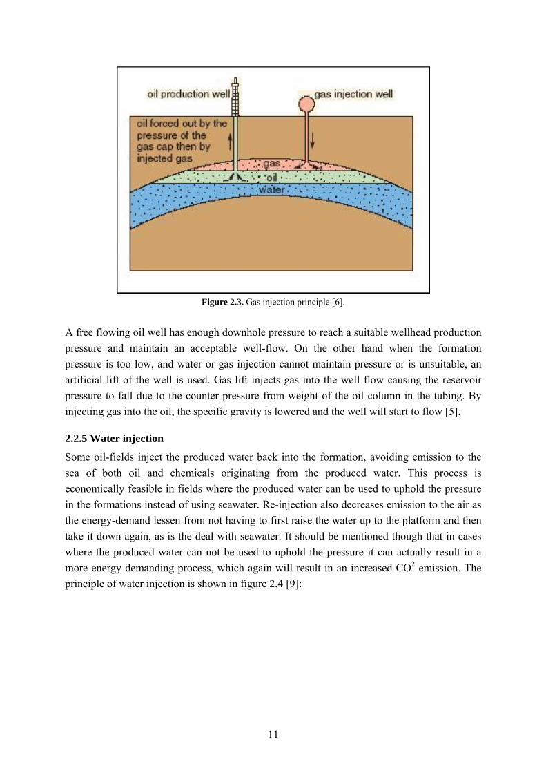
2.2.4 Gas- injection and lift When a well is drilled the hydrostatic formation pressure drives the hydrocarbons out of the rock and up into the well. When the gas, oil and water are extracted, the composition will change. The recovery of an oil reservoir is typically around 40%, but using certain measures one can take it up to about 70%. Gas or water injection is often used to maintain the reservoir pressure and in this way force the oil toward the production wells as illustrated for injection of gas in figure 2.3.

11

Figure 2.3. Gas injection principle [6].

A free flowing oil well has enough downhole pressure to reach a suitable wellhead production pressure and maintain an acceptable well-flow. On the other hand when the formation pressure is too low, and water or gas injection cannot maintain pressure or is unsuitable, an artificial lift of the well is used. Gas lift injects gas into the well flow causing the reservoir pressure to fall due to the counter pressure from weight of the oil column in the tubing. By injecting gas into the oil, the specific gravity is lowered and the well will start to flow [5].

2.2.5 Water injection

Some oil-fields inject the produced water back into the formation, avoiding emission to the sea of both oil and chemicals originating from the produced water. This process is economically feasible in fields where the produced water can be used to uphold the pressure in the formations instead of using seawater. Re-injection also decreases emission to the air as the energy-demand lessen from not having to first raise the water up to the platform and then take it down again, as is the deal with seawater. It should be mentioned though that in cases where the produced water can not be used to uphold the pressure it can actually result in a more energy demanding process, which again will result in an increased CO2 emission. The principle of water injection is shown in figure 2.4 [9]:

12

Figure 2.4. Water injection principle [6].

13

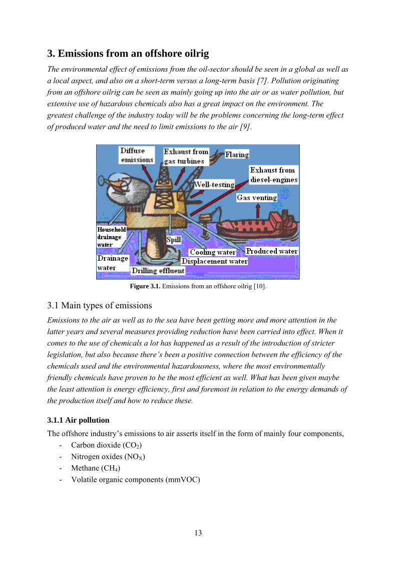
3. Emissions from an offshore oilrig The environmental effect of emissions from the oil-sector should be seen in a global as well as a local aspect, and also on a short-term versus a long-term basis [7]. Pollution originating from an offshore oilrig can be seen as mainly going up into the air or as water pollution, but extensive use of hazardous chemicals also has a great impact on the environment. The greatest challenge of the industry today will be the problems concerning the long-term effect of produced water and the need to limit emissions to the air [9].

Figure 3.1. Emissions from an offshore oilrig [10].

3.1 Main types of emissions Emissions to the air as well as to the sea have been getting more and more attention in the latter years and several measures providing reduction have been carried into effect. When it comes to the use of chemicals a lot has happened as a result of the introduction of stricter legislation, but also because there’s been a positive connection between the efficiency of the chemicals used and the environmental hazardousness, where the most environmentally friendly chemicals have proven to be the most efficient as well. What has been given maybe the least attention is energy efficiency, first and foremost in relation to the energy demands of the production itself and how to reduce these.

3.1.1 Air pollution

The offshore industry’s emissions to air asserts itself in the form of mainly four components, - Carbon dioxide (CO2) - Nitrogen oxides (NOX) - Methane (CH4) - Volatile organic components (mmVOC)

14

where the emissions of CO2 and NOX mainly are a result of combustion of natural gas in turbines used for power generation. Loading of oil is the main contributor to mmVOC emissions. Emissions to air increase proportionally with the production rate. [9]

Flaring, which is defined as controlled combustion of gas justified as a cause of safety, is also a significant contributor to airborne emissions, and probably the simplest to measure. The flare subsystems includes flare, atmospheric ventilation and blow down and has the purpose of providing safe discharge and disposal of gases and liquids [5].

Flaring is not a part of the normal operation of a plant, but may still occur as a result of: - Spill-off flaring from the product stabilization system. - Production testing. - Relief of excess pressure caused by process upset conditions and thermal expansion. - Depressurisation either in response to an emergency situation or as part of a normal

procedure. - Planned depressurisation of subsea production flowlines and export pipelines. - Venting from equipment operating close to atmospheric pressure.

3.1.2 Water pollution

From an offshore oil-rig there are emissions of both oil and chemicals to the sea. Some oil will go out with the water as part of planned operation because it is inevitable and/or because it serves the production [9]. Water is also a product co-produced with oil and gas from hydrocarbon reservoirs, often referred to as produced water, which has to be purified before re-remittance into the sea.

Water production is normally low from new fields but as the field matures more water is produced as a result of changed reservoir conditions and water being injected to the reservoir for pressure support. For older fields well streams containing 90% water or more are not uncommon and correspond to greater difficulties with oil in emitted water [11]. A closer look at this problem will be given in chapter 4.

3.1.3 Use, classification and emission of chemicals

The use of chemicals on an offshore oil-rig is found in drilling and well-maintenance, provided in the production and processing itself, or being part of the piping processes and transportation. In addition it has to be taken into consideration the chemical substances existing naturally in the reservoirs [9].

15

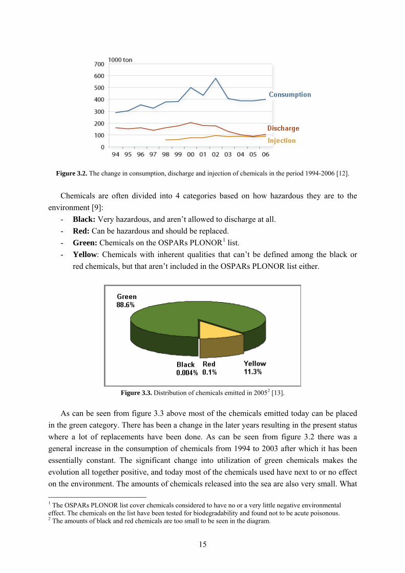
Figure 3.2. The change in consumption, discharge and injection of chemicals in the period 1994-2006 [12].

Chemicals are often divided into 4 categories based on how hazardous they are to the

environment [9]: - Black: Very hazardous, and aren’t allowed to discharge at all. - Red: Can be hazardous and should be replaced. - Green: Chemicals on the OSPARs PLONOR1 list. - Yellow: Chemicals with inherent qualities that can’t be defined among the black or

red chemicals, but that aren’t included in the OSPARs PLONOR list either.

Figure 3.3. Distribution of chemicals emitted in 20052 [13].

As can be seen from figure 3.3 above most of the chemicals emitted today can be placed

in the green category. There has been a change in the later years resulting in the present status where a lot of replacements have been done. As can be seen from figure 3.2 there was a general increase in the consumption of chemicals from 1994 to 2003 after which it has been essentially constant. The significant change into utilization of green chemicals makes the evolution all together positive, and today most of the chemicals used have next to or no effect on the environment. The amounts of chemicals released into the sea are also very small. What 1 The OSPARs PLONOR list cover chemicals considered to have no or a very little negative environmental effect. The chemicals on the list have been tested for biodegradability and found not to be acute poisonous. 2 The amounts of black and red chemicals are too small to be seen in the diagram.

16

should be mentioned, is that even though some chemicals have not proven to have an impact on the surroundings separately, little is known about the effect of them in connection to each other [9].

3.1.4 Energy utilization in the production and power generation

An offshore oil-rig consumes large amounts of energy, which leads to indirect environmental impacts if the energy is not renewable. Especially the turbines running the compressors in the gas-train depend strongly on energy supply, which is commonly supplied through combustion of the available oil and gas products. A large amount of fuel is necessary for running the turbines, and the efficiency is quite poor.

The instalment of gas-turbines as a power source offshore is now met by the alternative of using an on-shore electrification of the shelf. This is performed by the delivery of a direct current using the so called HVDC (High Voltage Direct Current) light technology and makes it possible to distribute high voltage power using both subsea and subterranean wires. Arriving at the platform the power is changed into alternating current. This technology has been used on the Troll A platform outside Bergen and is also planned on being inducted on the Valhall platform in 2009. For the Valhall platform the introduction is expected to result in a reduction in CO2 emissions of 300.000 metric tonnes a year, which corresponds to the emissions resulting from the power consumption of 30.000 households. The installation also provides reduced maintenance costs, as well as reduces the total weight of the platform equipment. The electrification can contribute to more efficient energy utilization as well as reduced production costs [14].

The problem is that the implementation costs, and calculations made by the Norwegian Petroleum Directorate show that the expenses of the measures necessary to electrify the shelf will be high compared to the CO2- and NOx- taxes of today as well as the expected international CO2 quota price and recommend that existing facilities should not be modified. Looking at the efficiency of the offshore power plant it is in general less efficient than an on-shore energy plant, but the land based plants also vary in efficiency with for example location. From a strictly environmental aspect the introduction of electrification would still be advantageous despite the cost, but a point worth mentioning is the energy accessibility. Energy has to be supplied to the shelf and if the energy is not provided from renewable sources there will be an indirect environmental impact. The conclusion is therefore that unless the shelf is electrified with pollution free energy the overall CO2 emission might remain the same. An interesting current aspect is the possibility of combining the electrification with windmills along the coast or even offshore [15].

17

3.2 Environmental impact caused by the emissions Emissions from the oil- and gas- sector are responsible for a large percentage of the total Norwegian pollution contribution. The effect of the emission of pollutants to the air as well as the sea should be looked at in two perspectives, a short term as well as a long term one. Emissions of NOX contribute to overfertilisation, acidification and ground level ozone as well as NO2 emitted. Emissions of NMVOC3 in combination with NO2 result in ground level ozone formation. CO2 and CH4 on the other hand have shown to be contributing to the greenhouse effect and consequently global warming. Emission of these gases which have large residence times in the atmosphere has a long term effect [9].

Acute emissions often give a clear picture of the resulting environmental effect as well as the effect it has on the surrounding flora and fauna. There is a larger uncertainty when it comes to the long term effect of the emissions, the reason being the low concentration of several compounds over the same time period. The composition of the emissions also varies significantly [9].

Despite stricter control and legislation as well as the introduction of new technologies, pollution originating from the oil-industry will probably continue to be at a high level as long as production is still economically feasible. The introduction of less hazardous chemicals is one of the measures that has had a positive influence from an environmental perspective, but a lot of work remains regarding handling emissions to air and the increasing amount of produced water [9].

3 NMVOC is the abbreviation for non-methane volatile organic compounds.

18

4. Water purification treatment The demand of zero emissions offshore has been a great motivation in the development of new water treatment technologies. International regulations of produced water discharges to sea have also been enforced to a greater strength in the latter years resulting in increased focus on optimizing produced water treatment [11]. On older installations, produced water treatment might be by means of large-volume plate separators and gas flotation units. On newer installations, and when replacing equipment on older platforms de-oiling hydrocyclones followed by smaller degassing units are normally installed.

4.1 Oil-water separation Oil and water separation offshore can be divided into three stages: A rough separation of oil, gas and water provided by the separator, further removal of water from the produced oil and oil removal from water ahead of discharge back into the ocean or injection into a reservoir. The latter one is of highest interest wanting to minimize the environmental impact, and is provided a further discussion in the following section. The discharge of produced water to the sea has to follow strict governmental restrictions presenting the lower limit of oil-content of 30 mg/l in the released water. The oil-companies own demands are often more stringent operating with a limit of about 25mg/l. As the old oil-wells are depleted and the oil-sector is expanding its production into new areas important for fishing and fish reproduction even lower limits of minimum oil-releases will be introduced [16].

Crude oil has densities in the range of 800-900 kg/m3 whereas sea-water has a density around 1030 kg/m3. Since one of the phases is hydrophilic and the other lipophilic the phases are immiscible and will form two separate layers where the oil will be “floating” on top of the water phase separated by an emulsion. This is illustrated in figure 4.1 below:

Figure 4.1. The layers inside the separator.

The problem of emulsion formation will be assessed in the following section.

19

4.1.1 The problem of emulsion formation

An emulsion is a quasi-stable4 suspension of fine drops of one liquid dispersed in another [17]. Emulsion formation prevents separation in a reasonable time [5].

There are two requirements in emulsion forming: 1. Two immiscible liquids 2. Enough agitation to disperse one liquid into small drops

Turbulence or agitation is often the triggering factor of emulsion formation as the shear forces break the dispersed liquid up into many small droplets. The natural tendency will still be coalescence as long as there isn’t an emulsifying agent or emulsifier present preventing it. This agent will most often be a surface active agent or surfactant which because of its amphipathic5 quality stabilizes the emulsion by forming an interfacial film around the immersed drops [17].

In the petroleum industry emulsions are often divided into water in oil emulsions, and oil in water emulsions, the latter of the phases being the continuous one. The type of emulsion formed depends primarily on the emulsifying agents present and, to a lesser extent, on the relevant amounts of aqueous and oil phases. On the basis of the environmental fundament of this thesis oil in water emulsions are the most interesting [17].

Emulsions possess interfacial energy and are therefore thermodynamically unstable. This means that they are possible to separate, something for which there exist several mechanisms: Sedimentation or creaming, aggregation, and coalescence. The rate at which the dispersed drops coalesce and “break” the emulsion depends on several properties of the substances: The interfacial film, existence of electrical or steric barriers, viscosity of the continuous phase, drop size, phase volume ratio, temperature, pH, age, brine salinity, and type of oil [17].

4.1.2 Coalescence and drop splitting

Drops dispersed in another fluid have a natural tendency of coalescing as long as no stabilizing agents are present, but prominent fluid motion may initiate the counterweight of drop splitting [17]. Coalescence is the term describing droplet growth as small drops merge together when they come in contact with each other. If this occurs repeatedly over time, a continuous phase will form.

For coalescence to occur the drops have to collide. It is reasonable that larger drops are more likely to do so, with each other as well as with smaller drops as they have a larger surface area and therefore occupy a greater range of the container volume. Considering a fixed control volume, the residence time of the suspended matter is also of great importance.

4 A quasi-stable suspension is an unstable suspension 5 An amphipathic molecule has one hydrophilic (soluble in water) part and the other one lipophilic (soluble in oil).

20

The longer the drops are introduced to the possibility of colliding with each other the more of them will [17].

The effect of coalescence should be weighed with the effect of turbulence or agitation present in the oil-water mixture as it will work as an opposition breaking up the drops into smaller droplets [17].

Interfacial or surface tension tends to coalesce dispersed droplets. Many droplets dispersed in a continuous phase have a very large collective interfacial area. As the particles coalesce, the total interfacial area is reduced. Surface tension can be defined as the work required to increase the interfacial area by one unit, where the work also represents the energy potential available to reverse the process and produce a smaller interfacial area. The natural tendency is therefore for coalescence to occur. Small drops will combine and decrease the interfacial area, as well as the total surface energy and the Gibbs free energy of the system as long as no stabilizing forces are present [17].

4.1.3 Population balances Population balance modelling (PBM) is a mathematical modelling technique used to describe population dynamics [18]. The reason for wanting to use population balance modelling on a particulate system is that the distribution of internal properties in a system affects product quality. In PBM the system is divided into regions where there is a marked change in properties from one region to the next. The number of compartments used in a model is defined by the number of regions physically identifiable in the system [4].

In oil and water separation PBM can be used to predict the mean size of drops by assuming coalescence and breakage are the key mechanisms [18].

A suggestion to an overall population balance equation for the rate of change in number of drops of characteristic size, v, through the dynamics of coalescence and breakage is described below [18]:

0

0

1

2

3

4

( ) 1 ( , ) ( ) ( ) 2

( ) ( , ) ( )

+ ( ) ( ) ( )

( ) ( )

vdn v v u u n v u n u dudt

n v v u n u du

b v w S w n w dw

S v n v

β

β∞

= − −

−

−

∫

∫ (4.1)

21

where ( , ) is the frequency of collisions between drops of volume and , ( ) and ( ) are number concentrations of volume and respectively, ( ) is the breakage probability density function

v u u v n v n uv u b v w

β

of particles of volume into particles of volume , ( ) and ( ) are selection rates of particles of volume , and respectively and ( ) is the number concentration of particles of volume .

w v S v S wv w n ww

The evolution of ( ) is a result of the four mechanisms shown in the equation 4.1: 1. The increase in concentration of drops of volume due to coalescence, when collision between dr

n vv

ops of volume - occurs (coalescence birth). 2. The decrease in concentration due to collision of drops of volume with any other drop (coalescence death). 3. The increase in concen

v uv

tration when larger drops of volume break into drops of volume (breakage birth). 4. The decrease in concentration when drops of volume break into smaller drops (drop death)

wv

v.

To compete a population balance model for oil from water separation one would probably have to account for the spatial distribution in addition to the particle size distribution increasing the complexity level of the model even further [19].

Any model to be used in industrial purposes has to be validated using experimental data. Gathering good experimental data of the population density distribution is difficult [4]. In conclusion accounting for the spatial distribution of drops would increase model realism, but the increased level of complexity would result in a model too impractical for industrial application [4].

4.2 Different types of equipment available Depending on the purpose and the installation in question different types of applications can be used to reduce the amount of oil in water, some of which will be given a short introduction in this section.

- Gravity Separators: Provides separation based on the specific gravity difference between the oil and the wastewater, and separation efficiency depends highly on the residence time of the dispersed fluid in the tank. The tank has its greatest efficiency in removing bigger amounts of oil, and can not be the only measure in a water cleaning system fulfilling governmental restrictions.

- Oil skimmer: Separates oil floating on water [20]. - Plate coalescer: Uses plates to capture the oil drops, which glides of as a film [20]. - Flotation tanks/cells: Uses dissolved air flotation dissolving air in the waste water

under pressure and then releasing the air at atmospheric pressure in the flotation tank. The released air forms tiny bubbles which adhere to the suspended matter causing it to

22

float to the surface of the water where it is removed by a skimming device. The measure makes removing very small droplets possible [21].

- Hydro cyclones: The most important measure used in the industry today. As a result of its importance and extensive use the advantages and disadvantages are provided a short discussion in the following section, and more theory presented in chapter 5.

4.2.1 Advantages and disadvantages of hydrocylones There are mostly advantages related to the use of hydrocyclones as the main step in a water purification system, but also some disadvantages. In this section both will be given a closer look. The main advantages resulting from the use of hydrocyclones are high capacity, simplicity and small space requirement, which are major concerns on an offshore facility [2, 22, 23]. Especially the limited space necessary to house the cyclone separates it from traditional systems consisting of flotation units and/or gravity based separators. These systems usually also require the use of costly chemicals and constant attention to be effective [3].

With hydrocyclones additional capacity is easily available as oil-fields mature and the water content increases. Another cyclone can simply be added to the existing system, an attribution referred to as add-on capacity [24].

Hydrocyclones complete separation in a few seconds, compared to minutes for traditional gravity separators [11]. They also respond rapidly to changes in conditions due to the low residence time [3, 24, 25]. Seconds after an upset the hydrocyclone will resume to normal performance, in comparison to the flotation cell which takes considerably longer to recover [3, 24].

The hydrocyclone is a very simple, compact system with no moving parts and as a result require minimum operator attention [24]. The maintenance level is also low, which is a benefit that comes with the use of hydrocyclones compared to other alternatives [23].

An offshore oil-rig is exposed to extreme weather conditions in its vulnerable position at sea, and platform movement tend to induce excessive turbulence on gravity separators and too much wave motion for effective skimming to be performed in flotation cells [3]. As the residence time is as short as 2 seconds in a hydrocyclone and at the same time the enhanced gravity field inside may reach 2,000 to 3,000g6 [11], the hydrocyclone is insensitive to motion and orientation [26].

Looking at some disadvantages problems found with surging flow and the importance of preciseness in operational conditions should be mentioned. One may also experience problems with the efficiency, but the use of chemicals has proven to be an effective solution to this in most cases. From an environmental perspective the use of chemicals should be avoided, but it is stated by Husveg [11] that proper maintenance and control can be enough to

6 g is a non-SI unit equal to the nominal acceleration due to gravity on Earth at sea level and is defined as 9.80665 m/s2 (32.174 ft/s2).

23

avoid the issue in some cases. Poor hydrocyclone efficiency is often attributed to unfavourable properties of the produced water or sub-optimal hydrocyclone design. Upsets in upstream production facilities, unfavourable configuration, poor maintenance or simply inadequate operational control may also result in poor performance [11].

On an offshore operation weight, space and manpower requirements are important, and provided good designs as well as a well suited operation, the use of hydrocyclones are still the best alternative found today separating dispersed oil from water [3].

4.2.2 Improved separation and alternatives In this section some alternatives or additional applications for oil and water separation are discussed.

- Vessel Internal Electrostatic Coalescer (VIEC): Enhances the separation process by the use of an electrostatic field [27]. By exposing an emulsion of water in oil to an electrostatic field, the water droplets contained in the oil phase will be coalesced into bigger droplets and separate more easily [28]. The VIEC is said to enhance the speed and efficiency of the separation process providing a more cost-effective and environmentally friendly production by reducing the need for chemical usage. VIEC has been implemented on the Heidrun platform among others and is illustrated in the figure 4.2:

Figure 4.2. Aibels VIEC [27].

- CTour: Uses condensates to remove oil mixed in and dissolved in the produced water.

Condensate is injected into the produced water, and function as an extraction agent which is added to the remaining oil after water and oil have been separated by ordinary measures. The condensate can be described as a solvent that turns the solved oil components in the water into oil droplets [29, 30]. The oil/condensate is almost entirely removed in the succeeding hydro cyclone processes [29]. CTour has been put to use in both the platforms Ekofisk and Statsfjord and a sketch of the typical process is presented in figure 4.3 [30]:

24

Figure 4.3. Sketch of a typical CTour process [31].

- Epcon Offshore Compact Flotation Unit (CFU): Combines principles such as gas

flotation, centrifugal- and coalescing effects. The separation process is aided by internal devices in the compartment and by a simultaneous gas flotation effect caused by the release of residual gas from the water. The unit has been tested on several platforms and is installed at the Brage platform, Troll C, Snorre and Heidrun as well as at Ekofisk J [32]. The principle of the Epcon offshore compact flotation unit is provided in figure 4.4:

Figure 4.4. Principle of the Epcon compact flotation unit [32].

25

- Oil-water separation on the seabed: Only the oil concentrated water component is lifted to the surface, while the bulk is re-injected into disposal zones or back into the reservoir to maintain pressure. The fact that water is removed at such an early stage result in an improved recoverability with low pumping power consumption based on the lower lift volume. The technique has been tested on the platform Troll C [2], and implemented on the Tordis field. A drawback with the use of re-injection is that it often means increased energy consumption resulting in an indirect increase in emission of CO2 to the air [16].

26

5. Hydro cyclones De-oiling hydrocyclones are prioritized technology for produced water treatment on offshore oil-producing platforms, where almost 90% of the facilities are equipped with hydrocyclone technology [8]. The reason being their superior qualitative performance as well as volumetric capacity, easy and reliable operation, low maintenance, and low utility requirements compared to traditional gravity separators.

5.1 Principle In this section the principle of hydrocyclone operation in separation will be provided. A hydrocyclone applies centrifugal force to a liquid mixture promoting the separation of heavy and light components. The separation is carried through converting incoming liquid velocity into rotary motion, directing the inflow tangentially near one end of a horizontal cyclonic body. This spins the entire contents of the cylinder, creating a centrifugal force in the liquid and a strong gravity field [33]. Fluids with different densities in the gravity field move in opposite directions radially. In a de-oiling hydrocyclone, the lighter oil phase migrates towards the centre of the vortex, and the heavier water phase is forced toward the cyclone wall.

Looking at the twofold vortex structure of hydrocyclones shown in figure 5.1 the hydrocyclone for separating light dispersions is designed such that the bulk of the flow, the more dense water phase, passes out underflow while allowing sufficient axial flow reversal to carry the central core of dispersion out the overflow exit. The main flow is in the underflow (> 90%), which is in contrast to the larger overflow when hydrocyclones are used to separate solids from a continuous liquid [23]. In a solid from liquid (s-l) separation the solids are the heavier and separated out of the underflow outlet.

27

Figure 5.1. Hydrocyclone principle [34].

One of the main characteristic differences between light dispersion hydrocyclones and the

original hydrocyclones separating solids from a liquid is the length. Hydrocyclones separating two immiscible liquids close in density are normally more than twice the length of solid-liquid hydrocyclones. The long and narrow shape provides a gentle tapering of the cone, more suitable to increase the residence time and maintain the high centrifugal force necessary to separate the extremely small oil droplets [3, 35].

The residence time in general is short, in the order of 2 seconds, and the hydrocyclone will therefore have fast dynamics [11].

In section 4.2.1 the term add-on capacity was presented as being able to simply ad on another hydrocyclone to the existing process structure. Most hydrocyclones consist of a cluster consisting of from 1 to 270 cyclone-liners which can be increased or decreased to match the water flow rate [36]. The liner configuration in a hydrocyclone is illustrated in figure 5.2:

28

Figure 5.2. Hydrocyclone liner configuration.

5.2 Hydrocyclone performance criteria In addition to its dependence on application design, hydrocyclone performance depends on appropriate operation of flow rate and flow split. The separation performance in a hydrocyclone, also referred to as the hydrocyclone efficiency, can be presented in several ways. A standard presentation is provided below: The hydrocyclone efficiency, η, is the separated mass of particles with diameter Dp divided by the total incoming mass of particles with diameter Dp [37],

,

,

oil overflow

oil inlet

mm

η = (5.1)

where m is mass and x is a fraction.

29

In reality stokes law7 governs hydrocyclone separation which means that hydrocyclone performance is depending on: Droplet size, temperature, differential density, inlet concentration, oil slugging, interfacial tension, chemical treatment, solids, and free and dissolved gas content. For each application most of these factors will remain constant and the operating variables of pressure drop will dictate efficiency. As a result of this as well as the short residence time empirical relationships providing hydrocyclone performance are often used for instance by Colman as what he referrers to as the effect of migration probability. This is the probability that a drop of a certain size leaving the hydrocyclone through the upstream axial outlet in the overflow [23].

These relationships are implemented on the assumption of an approximately static hydrocyclone. Often the effect is presented in terms of the cut size Dpc presented below: The cut size, Dpc, is the particle size where 50% of the particles follow the underflow whereas the other 50% follow the overflow. The resulting efficiency will be 0.5 [37]. The equations 5.2 and 5.3 provides a representation using the cut size originally provided by Rietema [38] and presented in turn by [35, 37, 39] and are made out for a solid-liquid hydrocyclone having the geometrical relationships provided in figure 5.3:

7 Stokes law gives an expression for the steady state settling/rising velocity. VS = g d2 (ρd – ρf) / 18 μf

30

Figure 5.3. Geometrical relationships of a hydrocyclone according to Rietema [38].

0.852

( = 0.177pc cp

D D PP

⎛ ⎞⎛ ⎞ ρΔρ − ρ) Δ ⎜ ⎟⎜ ⎟ ⎜ ⎟μ μ⎝ ⎠ ⎝ ⎠

i i (5.2)

1.852

cD PPQ⎛ ⎞ρΔ⎛ ⎞ρ Δ = 0.2⎜ ⎟⎜ ⎟ ⎜ ⎟μ ρ μ⎝ ⎠ ⎝ ⎠

(5.3)

where Dc = The diameter of the hydrocyclone [m]. Q = The suspension inflow [m3/s]. ΔP = The pressure drop [N/m2]. ρ = Liquid density [kg/m3]. ρp = Particle density. μ = dynamic viscosity of the fluid, [kg/(m s)] = [N s/m2][35, 39]

An oil concentration as high as possible in the overflow is a goal as it reduces the volumes of reprocessed water. However, to obtain high separation efficiency, some water will always exit in the overflow [11]. Complete separation of the phases going in to the hydrocyclone can not be obtained in one stage. One of the phases can be separated and taken from either the

31

under or the overflow of the cyclone while a mixture of the two phases appears at the opposite outlet. For a cyclone with a large overflow diameter and a small underflow diameter only the heavy phase can be delivered at the underflow and the mixture depleted in heavy phase at the overflow. Alternatively in the opposite scenario a cyclone with a large underflow and a small overflow can deliver light phase only at the overflow and the mixture depleted in light phase at the underflow. The Rietema equations 5.2 and 5.3 show that the efficiency in general is greater when using several small hydrocyclones compared to a larger one with the same pressure drop as the same performance is obtained for a smaller inflow [39]. Adding additional stages to the cyclone operation will help to overcome the limitations of the outlet diameter designs to some extent [22].

In separating oil from water, the two-folded vortex structure illustrated in figure 5.1 is essential and disturbances in the stability of the vortex may decrease separation efficiency [8, 11]. Vortex breakdown can result in the dispersion phase going out downstream with the clean water flow [23].

5.2.1 Flow rate Studying the Rietema equations 5.2 and 5.3 we find that the cut size depends only on the inlet flow rate and optimal operation of Qin is therefore important. In this section a discussion on the range of inlet flow providing optimal performance will be given. The flow rate entering the hydrocyclone must be in a certain range defined by Qmin and Qmax to obtain maximum efficiency as presented in figure 5.4 provided by Husveg as a re-illustration of Meldrums work [24]:

Figure 5.4. Hydrocyclone efficiency as a function of flow rate [8].

The separating forces in the hydrocyclone are weak at very low flow rates Qmin, as the

centripetal force is low [11]. A certain minimum flow rate is also necessary to set up the vortex motion and to produce the strong centrifugal separation forces required for optimum performance [24]. Hydrocyclone efficiency also reaches a maximum at a certain inflow Qmax

32

where a further increase in flow rate will cause a poorer separation as a result of increased droplet break-up and/or a lack of sufficient pressure gradients resulting in a reduction of the hydrocyclone axis [11, 22].

Also as the inflow to the hydrocyclone becomes large the already small residence time experiences a further decrease [11]. Meldrum in [24] explains the characteristic efficiency decrease at flow rates above Qmax as a result of either

a) a severe increase in droplet break-up due to excessive shear-forces and turbulence creating smaller droplets that are harder to separate. And/or

b) a lack of sufficient pressure gradients to drive the separated oil-core through the overflow. As flow rate increases, the core pressure approaches atmospheric pressure, and the pressure gradient decreases. The pressure available to drive the overflow stream is reduced which inhibits the overflow rate resulting in little and eventually no separation.

The second criteria, b), is considered to be the dominating restriction [24].

5.2.2 Flow split A flow split needs to be introduced in order to carry the oil-water separation into effect and also to maintain the internal flow structure of the hydrocyclone. Flow split, FS, is defined as presented below:

100 %overflow

inlet

QFS

Q= i (5.4)

where Q is volume flow [m3/s] In most de-oiling hydrocyclones, the overflow rate, Qoverflow, is only a few percent of the

inlet flow rate, Qinlet, (<10% [23]) [11]. Today it is usually maintained at 2-3%. [8] Results by Meldrum have documented a high oil-removal level with a flow split as low as 1%, but as the FS becomes too low, oil will be lost through the underflow [24].

It is shown by several [23, 24] that the effect of hydrocyclone separation as a result of flow split increases until it levels of and becomes essentially constant. This relationship is presented in figure 5.5 below which is a re-illustration of Meldrums work [24] provided by Husveg [4].

33

Figure 5.5. Typical hydrocyclone efficiency versus flow split relationship [8].

Meldrum claimed that an increase in the flow split above the plateau shown in figure 5.5

only yield marginal improvement. An improvement that is balanced off by the increased water reject volume separated out with the oil [24].

The efficiency relationship to the flow split remains unchanged for different inflow rates for a hydrocyclone [8]. Meldrum [24] stated that the required flow split would be influenced by the level of inlet contamination. For oil in water concentrations up to a few percent Colman in [23] concluded that separation efficiency was close to being maintained for increasing oil-concentrations at the inlet. On the other hand Beladi in [2] reported that an increase in oil content from 5-10% affected the maximum efficiency as well as the critical split, presented as a small drop in the FS plateau level. Hence the amount of dispersed oil entering seems to have an effect on the performance, but not at very low concentrations.

The flow split can be changed by either changing the size of the overflow orifice that is by design, or by changing the pressure gradient to the overflow orifice. Hence a control implementation can be used to alter the flow split [11].

The effect of the flow rate- and flow split criteria are closely linked. When the inlet flow reaches Qmax the efficiency falls off because it is not possible to maintain the optimum of 1% for the flow split [24].

34

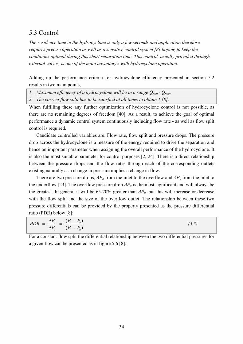
5.3 Control The residence time in the hydrocyclone is only a few seconds and application therefore requires precise operation as well as a sensitive control system [8] hoping to keep the conditions optimal during this short separation time. This control, usually provided through external valves, is one of the main advantages with hydrocyclone operation. Adding up the performance criteria for hydrocyclone efficiency presented in section 5.2 results in two main points, 1. Maximum efficiency of a hydrocyclone will be in a range Qmin - Qmax. 2. The correct flow split has to be satisfied at all times to obtain 1 [8]. When fulfilling these any further optimization of hydrocyclone control is not possible, as there are no remaining degrees of freedom [40]. As a result, to achieve the goal of optimal performance a dynamic control system continuously including flow rate - as well as flow split control is required.

Candidate controlled variables are: Flow rate, flow split and pressure drops. The pressure drop across the hydrocyclone is a measure of the energy required to drive the separation and hence an important parameter when assigning the overall performance of the hydrocyclone. It is also the most suitable parameter for control purposes [2, 24]. There is a direct relationship between the pressure drops and the flow rates through each of the corresponding outlets existing naturally as a change in pressure implies a change in flow.

There are two pressure drops, ΔPo from the inlet to the overflow and ΔPu from the inlet to the underflow [23]. The overflow pressure drop ΔPo is the most significant and will always be the greatest. In general it will be 65-70% greater than ΔPu, but this will increase or decrease with the flow split and the size of the overflow outlet. The relationship between these two pressure differentials can be provided by the property presented as the pressure differential ratio (PDR) below [8]:

( - ) ( - )

o i o

u i u

P P PPDRP P P

Δ= =Δ

(5.5)

For a constant flow split the differential relationship between the two differential pressures for a given flow can be presented as in figure 5.6 [8]:

35

Figure 5.6. Hydrocyclone differential pressures [8].

Husveg concluded that hydrocyclone efficiency is unaffected by transient flow rates

provided the hydrocyclone performance criteria are fulfilled [8]. Control is still important to make sure that the criteria are met at all times.

The downstream pressure control valves and internal reject orifices are used to control pressure drop and obtain acceptable quality of both the overflow and underflow streams. This must be accomplished at an adequately low hydrocyclone inlet pressure so as not to restrict well production with excessive backpressure [23].

A potential problem with control of the hydrocyclone can be that the control system is not reacting fast enough to changes in flow-rate. The control on the overflow stream will always lag behind that of the underflow [40]. This happens when the flow rate through a hydrocyclone increases. ΔPu immediately increases causing a temporary reduction in the PDR while ΔPo remains the same until the overflow control valve opens and increases ΔPo enough to restore the PDR set-point. If the PDR reduction during an increase in inflow becomes large enough, separation efficiency may temporarily drop off [8]. On the other hand if the inlet flow rate is decreased, as the flow rate drops, ΔPu immediately falls off and PDR increases until the overflow control valve closes and retrieves the set point reducing ΔPo. The flow split will increase temporarily and more water will be included in the overflow. Husveg reported indications of the hydrocyclone operating slightly more efficient during reduced flow rates compared with increased flow rates maybe due to an overall higher PDR resulting in a flow rate reduction[8]. Providing a overflow control reacting as fast as possible represents optimal control in this case [40]. The PDR deviations are a function of flow rate variations as well as control system response time [8].

Husveg stated [11] that in optimizing hydrocyclone performance, an operator may consider allowing operational interaction between hydrocyclones and separators, providing an alternatively routed oilstream, to increase hydrocyclone capacity and turndown and/or means to increase the capability of the hydrocyclone control system. Husvegs suggestion to an alternative control structure is presented in section 5.4.

36

5.3.1 Flow rate control There are two main issues of flow rate control which will be introduced in this section. In a typical deoiling application, the primary objective of a hydrocyclone flow rate control is to maintain a preset water level in an upstream separator by operation of the underflow control valve. A secondary objective is to maintain flow rates at the efficiency plateau of the hydrocyclones [11] [8]. In flow rate control differential pressures corresponding to Qmin and Qmax are often used in defining the controller output to the underflow control valve [8].

5.3.2 Flow split control The objective of flow split control is to maintain a flow split above the level ensuring optimal hydrocyclone efficiency. How this implementation is provided is presented in the following section. Resulting from the performance criteria flow split should be kept essentially constant as flow varies [2, 24]. This is controlled by the pressure differential ratio given in equation 5.5. By keeping the PDR constant as the flow varies, the flow split remains essentially constant, and hydrocyclone separation efficiency is maintained [26]. This is also valid in general for flow rates at the efficiency plateau where the hydrocyclone preferably is operated for best results. Increasing PDR means increasing the pressure gradient to the overflow, which gives a rise to the flow split according to equation 5.4. The relationship between the flow split and PDR is approximately linear [8, 11].

37

5.4 Hydrocyclone control structure. Knowing the performance criteria presented in section 5.2 as well as how the objectives can be attained through control presented in section 5.3 this section will present the control structure most commonly found offshore today as well as some alternatives. A typical control scheme is shown in the figure 5.7 presented below:

Figure 5.7. A typical control structure of the water treatment facility on an oil platform.

The underflow control valve, PVu, is operated by a level controller provided measurements of the water level in the separator. The overflow control valve, PVo, is used to control the flow split. This is done knowing the PDR from measurements of ΔPo and ΔPu provided by the pressure difference transmitters PDTo and PDTu respectively [8, 11].

The hydrocyclone is placed immediately downstream of the first-stage separator but upstream of the level-control valves, to maximize the available pressure driving force while minimizing high-shear areas that would cause particle break-up [24].

Other control schemes are found. Some of the earlier are simpler while others include additional equipment as pumps to support the necessary pressure [24]. The type of pump selected has a direct influence on the control system performance, as do pump control and valve location. Meldrum states that the pump recycle-valve and the pump itself are probably also responsible for creating a large number of smaller oil droplets than would otherwise occur.

Husveg in [8, 11] introduced a new control structure including operational flow rate boundaries (Qmin and Qmax) to the hydrocyclones by allowing for hydrocyclone-separator interactions. This control structure has two level controllers arranged in cascade mode

38

operating the underflow control valve, where the additional controller gets its set-point from the original but also includes a measurement of the underflow differential pressure PDTu. Husvegs control structure is illustrated in figure 5.8:

Figure 5.8. Husvegs improved control structure for the interacting system

between the separator and the hydrocyclone. Husvegs control structure provides a limitation to the signal coming from the water level transmitter LTw by providing the 2nd controller with the differential pressure of the underflow from PDTu. This pressure differential being an indirect measurement of the flow rate through the hydrocyclone can introduce limitations when needed. Hence when the signal from PDTu correlates to Qmax further opening of LVu is not allowed and excess water is carried over the weir. On the contrary, if the PDTu measurement correlates to Qmin the valve is forced to close, and an increase of the water to a certain level in the separator allowed [8]. The control structure proposed by Husveg increases the purity of water re-emitted to the ocean, but also allows more water to go out with the oil and would therefore work best as an implementation to the first of a series of separators.

39

6. Modelling the separator The following chapter describes the modelling of the separator, provides the main assumptions and the resulting mathematical structure followed by some cases validating the implementation. The separator has the purpose of processing the well flow into the clean marketable products: oil, natural gas and condensates. The separator model is provided on a basis of a general three phase separator including a weir separating the two liquid outlets. In this thesis the focus is on oil from water separation and the effect of the gaseous phase as well as the quality of the oil product will be neglected. The model is provided for process control purposes and the objective of control is therefore also important.

The level of accuracy for the model has to be compared to the time a simulation requires. It is also important to provide the model base on applications found commonly offshore today as the adaptation to reality and as a result the applicability of the model to a given case increases.

Energy balances have been neglected assuming temperature changes do not have a significant effect studying the flow though the system for control purposes. Also the already existing model of the oil- and gas-train does not include energy balances, and a coupling of the two models would as a result be easier. The assumption is provided a short discussion in appendix C.

The model is made using Simulink, Matlab, which is what ABB uses and the modelled equipment could be included in their Simulink library as a result. Using Simulink the process flow and the operation of the control system is also easily viewable.

The Simulink model is found on the disc attached to the original thesis and a copy of the script providing the separator coding is provided in appendix D.1.

6.1 Modelling the residence time using a reactor flow parallel The characteristics of the flow of dispersed oil in water are essential in choosing which properties should be included in determining the separation efficiency. In this section a continuous stirred tank reactor (CSTR) parallel was compared to a plug flow reactor (PFR) parallel approach as well as a series of CSTRs trying to find the best way of modelling the residence time. But first a short introduction to the liquid mass balances will be given.

6.1.1 The separator fluid mass balances The liquid flow through the separator will, for the purpose of this work, be considered to consist of one pure flow of oil-product and one contaminated water flow including dispersed oil. This is illustrated in figure 6.1 below:

40

Figure 6.1. The separator mass balances.

where the pure oil flow is presented in the top control volume and the contaminated water flow in the control volume at the bottom. As dispersed oil is separated out from the water-phase it joins the oil-phase. The effect at which this separation occurs will be presented in the succeeding sections after a model of the flow is found.

6.1.2 The reactor alternatives The alternatives of using a simple CSTR, a PFR or a series of CSTRs are discussed in this section and as a result of the change in concentration of the oil drops through the separator the simple CSTR is disregarded as an option. In a plug flow reactor, as the one shown in figure 6.2, the reactants are continuously consumed as they flow down the length of the reactor.

Figure 6.2. Plug flow reactor.

Deriving the design equations for the PFR it is assumed that the concentration varies continuously in the axial reaction on its way from the inlet to the outlet. As the reaction rate is a function of concentration, it too will vary axially. The expression for the average PFR residence time τ can be found from the expression of the total water volume, Vw [41],

41

= ( ) t t t

w ktt

V q d qθ θ−τ−τ

≈ Δ ∑∫ (6.1)

where qk is the inlet flow at time t = k and Δt is the sample time for the flow measurement. The single, ideal, CSTR shown in figure 6.3 is generally modelled as having no spatial

variations in concentration, temperature or reaction rate through the vessel as a result of a well mixed operation.

Figure 6.3. Continuous stirred tank reactor.

The reactor model is based on the assumption of the feed being completely mixed with the rest of the reactor content and the average residence time in the CSTR is found from the mean flow, qmean, going through. The expression for the total water volume in a CSTR gives the average residence time,

= w meanV qτ i (6.2)

The flow of dispersed oil drops through the separator varies in concentration through the tank as a result of coalescence and drop-splitting. The residence time of the drops will vary, but not to the extent of what is described by the CSTR model. A change in the inlet- or outlet- flow will cause a dramatic change in the average residence time for the CSTR as it depends only on the present value of the two flows. In reality the effect of the flow variance will occur gradually if the change is permanent or be negligible if the period is short enough. This can be illustrated picturing an oil drop that is close to reaching the separator outlet. If there is a sudden increase in the inflow, the mean flow estimated for the CSTR will increase, implying a sudden decrease in the average residence time. The drop which is already near the exit may experience the new estimation of the residence time to be shorter than the period already passed, which is wrong. The simple CSTR is therefore not a sufficient alternative.

Another alternative is as a series of small CSTRs of equal volume. Increasing the number and decreasing the volume of each CSTR the characteristics will approach and eventually become identical to those of the PFR. This alternative will include the presence of back mixing that might be present as the flow cannot be viewed as strictly laminar. In modelling, the CSTR also has an advantage of mathematical simplicity which may provide a faster simulation important for engineering purposes [41].

42

A problem with the series-CSTR approximation is the search for the optimum number of CSTRs as well as knowing the flow between the tanks. A possible solution to the last issue might be an average, as presented for a series of four CSTRs in figure 6.4:

Figure 6.4. An average of the flow when modelled as a series of four CSTRs.

The PFR model finishes in a sufficient number of seconds and the mathematical

simplicity of the CSTR is therefore not that important. A comparison of the CSTR to the PFR implementation is presented in section 6.3 validating the separator model structure. The series CSTR has not been tested but would probably provide a sufficient alternative, but as the PFR model finished in sufficient time it was kept as a measure of the residence time.

6.2 Variation of concentration A reactor approximation consisting of either a PFR or a series CSTR provides the best picture of the dispersed oil flow going through the separator as a result of the oil concentration varying through the tank. How the concentration varies depends on the forces on the single drop in the water, the drop size and coalescence and make up the basis of separator efficiency. The oil drop dispersed in water is influenced by the effect of several forces shown in figure 6.5:

43

Figure 6.5. The forces on a dispersed oil drop in water.

Gravity is pulling the drop downwards while buoyancy as the counterforce will be driving the drop upwards. In addition the surface tension is working on the liquid interface. Most important is the effect of the density differences though, giving the oil drop a movement in the upward direction as it is lighter than the surrounding water.

At the start of the separation the oil content in the water is the largest and as a result the separation will be as well. The more oil drops present in the water the greater the effect of coalescence described in section 4.1.2 and also the probability of a single drop reaching the oil phase.

Turbulence has to be present for drop-splitting to occur. As the liquid volumes are quite large in the separator and the dispersed oil volume a lot smaller than the water volume the effect of fluid motion is assumed to be limited. The natural tendency will be coalescence as the effect of surface tension, while trying to minimize surface area and maintain the drop shape, shows a greater resistance to splitting than to merging of drops. This is assuming there are no emulsifiers present stabilizing the drops in the emulsion. Coalescence is assumed the most important effect on concentration variation of the oil drops through the separator and can be described as a second order reaction of the form, A + A B (6.3) where the As represent small oil drops coalescing into a larger one B.

If the drops coalesce or not, or how many times a drop merges with another on its way towards the emulsion depend on several factors. The most important are presented in figure 6.6 illustrating some of the different paths an oil drop can take through the separator and given a short discussion in the succeeding sections 6.2.1- 6.2.3.

44

Figure 6.6. An illustration of the different paths an oil drop can go through the separator.

The oil drop following the paths a, b, c and d has the same size. Path a and d show the effect of the height in which a drop enters the separator on the path to the emulsion, whereas e show the effect of drop size. a, b and c provides a description of the effect of residence time.

6.2.1 Initial height of the drop The closer the drop is to the emulsion initially after entering the separator, the shorter the road to separation is. The height of the water-phase at which the drop enters decides how far away it is from reaching the oil phase and hence the length of the path to the emulsion.

The initial height also has an effect on coalescence as it says something about the probability of a drop meeting another on its path to the emulsion. The further the distance the drop has to travel the larger the possibility it has of colliding with another resulting in a merge between the two. In the extreme scenario of a drop entering at an initial height very close to the height of the emulsion layer the probability of coalescence is minimal.

6.2.2 Inlet drop size The larger the drop the faster the separation is. The larger drops have a greater speed in the direction of the emulsion and are also the most likely to get separated as the effect of surface tension decreases with a decrease in effective

45

surface area. The smaller drops on the other hand are more likely to remain in the water phase all the way through the separator and exit with the water outlet.

Separation efficiency of oil drops dispersed in water depends on the oil drop composition at the inlet. The inlet composition changes as the number or the size of the drops changes. As a result five compartments were introduced inspired by the population balance theory, presented in section 4.1.3, and provided a number from 1-5 and a mean drop size. The smallest drops were placed in compartment 1 and the mean drop sizes gradually increased for the succeeding compartments providing compartment 5 with the largest drops. The number of compartments introduced was made on the assumption of sufficiently being able to study sizes either close together or in a greater range having five different mean drop sizes. The number of compartments can be increased in the coding or decreased by simply providing the same mean drop size for several compartments.

The introduction of the compartments takes place at the separator inlet where each compartment of dispersed oil drops is presented as a fraction of the water inlet flow.

6.2.3 A practical model of coalescence dynamics The longer the drop is in the separator the greater the possibility of it coalescing and/or reaching the emulsion. The drops entering the separator can be of one size or up to five different sizes depending on how many compartments are put to use. From now on an assumption of utilization of all the five compartments representing different mean drops sizes will be made. With several sizes present one would expect a possible transition of drops from one compartment to another as the drop sizes increase within a compartment due to coalescence. This is illustrated in figure 6.7:

46

Figure 6.7. Coalescence of drops within the compartments resulting in a transition of

drops to the compartments housing the greater drop sizes. As the drops coalesce a general movement of oil from the compartments containing the smallest drops to the ones containing the larger will take place.

Taking the drop size distribution into consideration coalescence can be presented as a higher order reaction of the form, A + A B B + B C C + C D D + D E E + E F A + B + C + D + E F (6.4) where the letters A – F represent drops of different sizes coalescing into larger drops. In the presentation in 6.4 only drops within a compartment coalesce, but merging of drops of different sizes will also exist. Some examples are provided below: A + B A/B B + D C D + E D/E and possibly coalesce themselves A/B + B C- Including the numerous possibilities in which drops can coalesce presented in the previous examples would result in a very complex model. For the purpose of process control including coalescence is an advantage to keep the model realistic, but an approximation of 2nd order characteristics where coalescence is assumed only to take place within a compartment is assumed to be sufficient, and was used in the succeeding estimation of separator efficiency.

47

The characteristics cover the effect of coalescence depending on the residence time. The effect of the height of the drop at the inlet is neglected as it is the bulk phase and not a single drop that is studied. The effect of drop size on the other hand has to be included in addition to the residence time dependence to provide the full picture of separation performance including the effect of separation for the different compartments. This will be shown in section 6.2.5, but first a closer look at the second order reaction dynamics.

6.2.4 Second order dynamics Studying the change in concentration through the tank the dispersed oil drops in the PFR can be viewed as small batch reactors as illustrated in the figure 6.8, assuming only one reaction (A product) takes place and constant water volume.

Figure 6.8. A volume element moving through the separator. The mass balance for component A can then be written as

= - AA

dc rdt

(6.5)

and the reaction rate for the second order reaction in equation 6.3 given as 2 = A Ar k Ci (6.6)

48

Inserting equation 6.6 into the mass balance equation 6.5 and integrating provides second order characteristics for the concentration change through the separator presented in equation 6.7 [42].

[ ]

0

0

2

20

0

0

= -

1 = -

1 =

1 1 - =

A

A

A

A

AA

C t

AC

Ct

A C

A A

dc k Cdt

k dtC

k tC

k tC C

⎡ ⎤− −⎢ ⎥⎣ ⎦

∫ ∫

∫ ∫

i

i

0

1 1 = A A

ktC C

+ (6.7)

where CA is the dispersed oil fraction of the exiting water, CA0 is the initial dispersed oil fraction in the water entering and k is the rate constant of the reaction.

According to Johan Sjöblom [43], professor in surface and colloid chemistry and the Head of the Ugelstad Laboratory at NTNU, complete separation is estimated to take approximately 4 minutes assuming the oil is of the lighter sorts as the ones found in the northern sea. After this time period chemicals will be introduced providing a forced separation of the remaining dispersed oil. Complete separation is reached if 99.9% of the original input of dispersed oil is separated out according to Skogestad [44], that is CA = 0.001CA0 as CA describes the oil still dispersed in the water. This is the only data the model is based on, as data from an actual platform are difficult to obtain due to no online analyzer of the oil in water content. The model should be verified using experimental or process data before it is put to use, but in this thesis only a verification of the implementation will be provided.

6.2.5 Estimating separation efficiency The separation efficiency will depend on the effect of coalescence which again depends on the size of the droplets and on the residence time of the dispersed flow in the separator. In this section an expression for the total efficiency will be presented. Knowing the initial fraction of dispersed oil in the compartments and making the assumptions presented in the previous section, expression 6.7 can be rearranged to present the rate constant, k:

0.999 = 0.001 _ _ _ (4 60)

kx oil dispersed ini i i

(6.8)

where τ is the residence time. Knowing k, CA can be found, and will be the distribution of oil in the compartments still dispersed at the water outlet.

49

0

0

_ _ _ = = = _ _ _1 + 1 _ _ _

AA

A

C x oil dispersed inC x oil dispersed outktC k x oil dispersed in+ τi i

(6.9)

Each of the compartments have a rate constant k1, …, k5 as it depends on the fraction of oil dispersed of a given droplet size, see equation 6.8.

In addition a drop size efficiency ηds is introduced. The drop size efficiency’s relationship to the drop size is easily implemented into the separator mask, and should be provided for each separator to be studied based on experimental data. A default expression is provided, based on the assumption of a drop having a diameter equal to 100μm having an 80% drop size efficiency. The relationship is presented in the equation 6.10 below:

0.008 ds pDη = i (6.10)

where ηds is the drop size efficiency, Dp is the mean drop size and τ is the residence time. The mean drop sizes in the compartments are also provided default sizes which are presented in table 6.1 and are given on the base of knowing the drop sizes to increase in size from compartment 1 to compartment 5. The relationship providing the drop size efficiency as well as the mean drop sizes for the compartments are assumed, but applicable enough for use in control purposes and for testing the model implementation.

Table 6.1. The mean drop sizes in the compartments. Compartment 1 Compartment 2 Compartment 3 Compartment 4 Compartment 5

Dp [μm] 5 15 30 60 100 The drop size efficiency is provided as a minimum efficiency after a given residence time has passed. The flow of oil out with the pure oil, Qoil_a, as well as the flow of oil going still dispersed at the water outlet, Qoil_c from the drop size efficiency ηds are given below:

_ = _ _dsQoil a Q oil dispersedη i (6.11)

_ = (1 ) _ _dsQoil c Q oil dispersedη− i (6.12)

where Q_oil_dispersed is the flow of dispersed oil going in.

Including the total separation efficiency depending on both the residence time and the drop size the equation 6.9 can be re-written as,

0

0

(1 - ) = 1 + (1 - )

_ _ _ (1 - ) = 1 _ _ _ (1 - )

A dsA

A ds

ds

ds

CCktC

x oil dispersed ink x oil dispersed in

ηη

ηη+ τ

ii

ii i i

= _ _ _x oil dispersed out (6.13)

50

To maintain the possibility of complete separation as well as presenting the negligible effect of separation at very low residence times the total efficiency of separation was presented only for a range of the residence time. The drop size efficiency is provided as a minimum efficiency after a residence time of one minute has passed. Assuming that for residence times below one minute the effect of separation is negligible and further using Sjöblom’s statement of complete separation for residence times larger than 4 minutes [43] the range of residence time operation was provided and its effect on separation performance presented as:

0, 60 ( , ), 60 240

1, 240ds

sf s s

s

τη η τ τ

τ

<⎧⎪= ≤ ≤⎨⎪ >⎩

(6.14)

6.2.6 The residence time derived assuming PFR In this section, how the residence time, τ, depends on the PFR approximation is given. For a PFR with constant volume Vw we have that:

1 = ( ) t = t ( ... )t t

w t ttktt

V q d q q q qθ θ −τ−−τ−τ

≈ Δ Δ + + +∑∫ i (6.15)

where qk is the water inflow at t=k and Δt is the sampling time. The residence time τ is,

= tτ Δ τi (6.16)

where τ covers how many qk’s that has to be included to equal wVtΔ

.

In the figure 6.8 the drop can be seen as it moves upwards at the same time as it remains a part of the water volume element going through the separator.

An initialization period is needed when using the PFR approximation to make time for the first water volume element to go through the separator and one residence time to pass. This is done by providing an initial residence time,

0τ τ≥ .

Constant volume is assumed for the PFR approach. Hence, perfect level control is implied. As long as integral control is included the average level will be constant. The alternative would be a dynamic water volume. The equation 6.16 would then have to be adjusted to include another vector giving a mean water volume or else the effect of volume change would be greater than what is really the case. This mean water volume vector would be used to balance off the residence time as it takes into account that the changes in the volume does not happen suddenly with the change in level. Including water dynamics as described above was tested for the model but resulted in simulations running extremely slowly as a result of the many loops working within each other and was disregarded as an option. The assumption of constant volume is tested as part of the model validation in the next

51

section 6.3 providing good results. It should be mentioned, that not including the level dynamics, the model will not be able to study the effect of set-point changes in the controller.

6.3 Model validation Model validation on a dynamic level should check that the model is able to properly predict the transient behaviour of the system [4].

In this section four different cases will be used to verify the implementation of the separator model, which all are expected to decrease the separation performance.

1) Increasing in the water inlet. 2) Decreasing the mean drop sizes in the compartments. 3) Increasing the number of droplets. 4) Using a single CSTR parallel for calculation of the residence time. The assumption of constant volume used when implementing the PFR reactor model is also checked.

For the separator, the oil fraction still dispersed at the water outlet is provided as a measure of the efficiency, that is the higher the fraction of oil still remaining in the water, the poorer the separation. We will now investigate how this fraction changes when we consider the four cases listed above.

For the cases provided during the validation of the separator the residence time is assumed to be in the range of 1< τ <4 minutes where the equation 6.13 is valid.

52

6.3.1 Changing the water inlet Increasing the water inlet flow, expecting a poorer separation performance as a result of the residence time decreasing.

1300 1350 1400 1450 1500 1550 1600 1650 17000.04

0.05

0.06

0.07

Wat

er fl

ow a

t the

inle

t

1300 1350 1400 1450 1500 1550 1600 1650 1700

0.9

1

1.1

1.2

1.3

x 10-5

1300 1350 1400 1450 1500 1550 1600 1650 1700

2

4

6

8

x 10-6

time [s]

Oil

fract

ions

exi

ting

with

the

wat

er o

utle

t

Total oil fraction

Compartment 1Compartment 2Compartment 3Compartment 4Compartment 5

Figure 6.9. The effect on separator performance resulting from an increase in the water inflow.

Figure 6.9 shows that an increase in the water flow at the inlet decreases performance as expected. The decrease in separation performance is shown as an increase in the oil fraction still dispersed at the water outlet. The same is seen for the compartments. The increase in inlet water flow result in a shorter residence time which gives a poorer separation as presented in equation 6.13.

53

6.3.2 Changing the mean drop sizes in the compartments Decreasing the mean drop sizes in the compartments expecting poorer separation as the drop size efficiency decreases. The effect of the drop sizes in the separator is given as an additional drop size efficiency which depends directly on the mean drop size of a compartment, see equation 6.10.

When the residence time is less than one minute or more than 4 minutes the drop size efficiency does not have an effect on the separation performance. For the range where the performance varies with τ the drop size effect is still small as long as the residence time is of a sufficient size, see equation 6.13. A decrease of 50% for the mean drop size presenting each compartment was provided hoping to observe a viewable change. The results are presented in table 6.2.

Table 6.2. The drop size effect on the separator performance. Initial Final

Dp

[μm]

Oil fraction separated out

[10-6]

Dp [μm]

Oil fraction separated out

[10-6]

Change [%]

Compartment 1 5 0.02595 2.5 0.02597 0.07707

Compartment 2 15 0.10379 7.5 0.10387 0.07708

Compartment 3 30 0.64854 15 0.64905 0.07835

Compartment 4 60 2.5937 30 2.5935 0.2274

Compartment 5 100 5.8174 50 5.8306 0.2613

Total 9.1894 9.203 0.1480 A decrease in the mean compartment drop sizes decreases the drop size efficiency and should result in a poorer separation as a result of surface tension being larger for smaller drops as explained in section 4.1.2.

Table 6.2 shows that the total oil fraction still dispersed at the water outlet increases as a result of the decreased drop size efficiency. The same is true for the compartment oil fractions. The changes are still relatively small as a result of the residence time providing the main contribution to the separation performance.

The effect of the change is greatest for the largest drops which is natural as they have the largest decrease in size, and the drop size efficiency relationship being estimated as a percentage of the size.

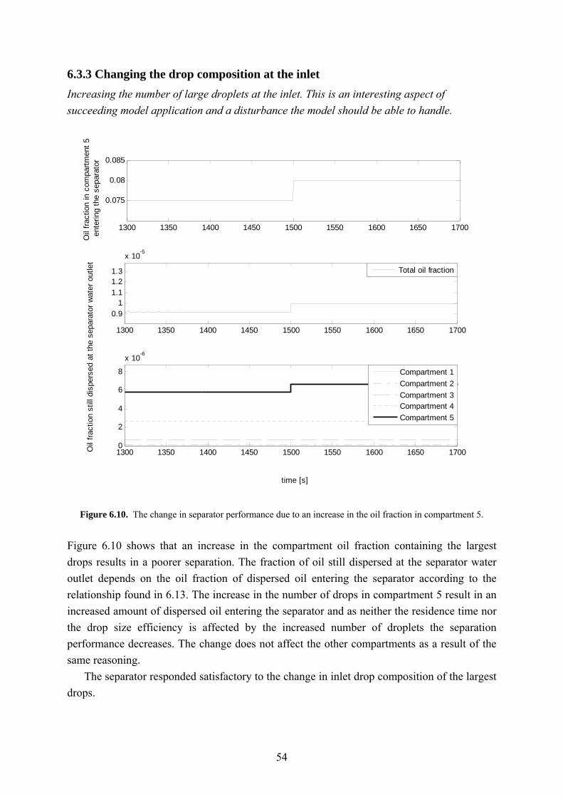
54

6.3.3 Changing the drop composition at the inlet Increasing the number of large droplets at the inlet. This is an interesting aspect of succeeding model application and a disturbance the model should be able to handle.

1300 1350 1400 1450 1500 1550 1600 1650 1700

0.075

0.08

0.085

Oil

fract

ion

in c

ompa

rtmen

t 5en

terin

g th

e se

para

tor

1300 1350 1400 1450 1500 1550 1600 1650 1700

0.91

1.11.21.3

x 10-5

1300 1350 1400 1450 1500 1550 1600 1650 17000

2

4

6

8

x 10-6

time [s]

Oil

fract

ion

still

dis

pers

ed a

t the

sep

arat

or w

ater

out

let

Compartment 1Compartment 2Compartment 3Compartment 4Compartment 5

Total oil fraction

Figure 6.10. The change in separator performance due to an increase in the oil fraction in compartment 5.

Figure 6.10 shows that an increase in the compartment oil fraction containing the largest drops results in a poorer separation. The fraction of oil still dispersed at the separator water outlet depends on the oil fraction of dispersed oil entering the separator according to the relationship found in 6.13. The increase in the number of drops in compartment 5 result in an increased amount of dispersed oil entering the separator and as neither the residence time nor the drop size efficiency is affected by the increased number of droplets the separation performance decreases. The change does not affect the other compartments as a result of the same reasoning.

The separator responded satisfactory to the change in inlet drop composition of the largest drops.

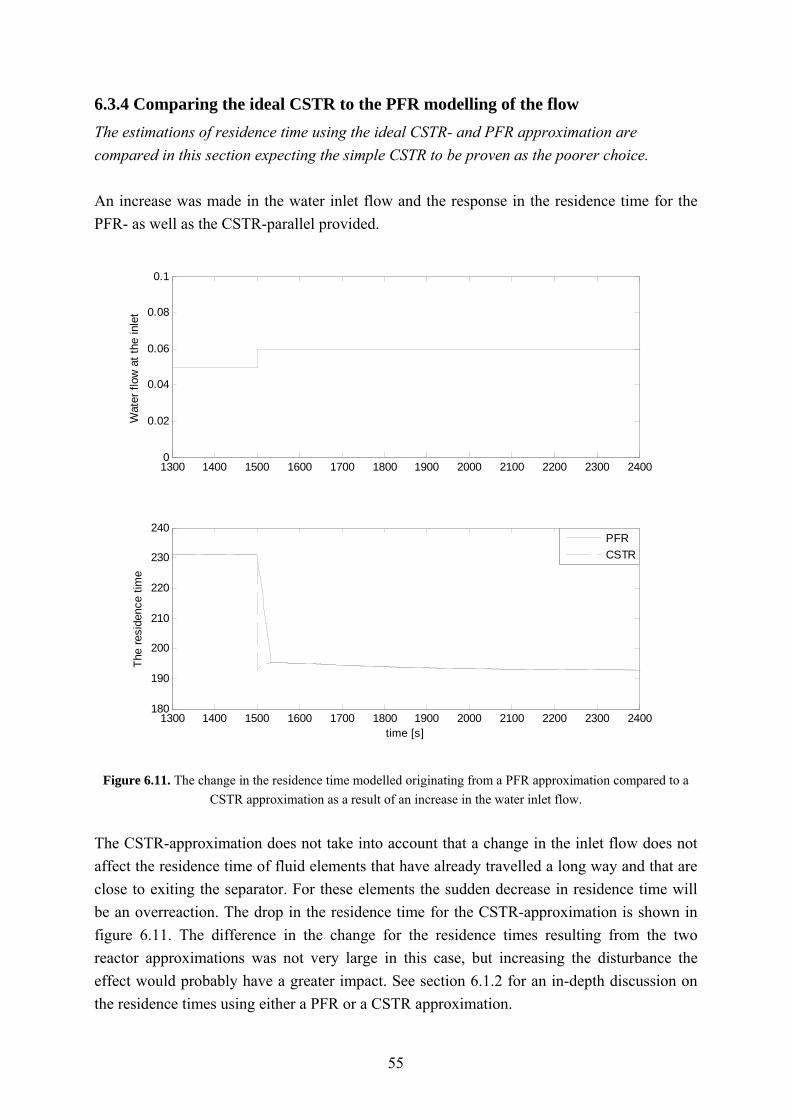
55

6.3.4 Comparing the ideal CSTR to the PFR modelling of the flow The estimations of residence time using the ideal CSTR- and PFR approximation are compared in this section expecting the simple CSTR to be proven as the poorer choice. An increase was made in the water inlet flow and the response in the residence time for the PFR- as well as the CSTR-parallel provided.

1300 1400 1500 1600 1700 1800 1900 2000 2100 2200 2300 24000

0.02

0.04

0.06

0.08

0.1

Wat

er fl

ow a

t the

inle

t

1300 1400 1500 1600 1700 1800 1900 2000 2100 2200 2300 2400180

190

200

210

220

230

240

time [s]

The

resi

denc

e tim

e

PFRCSTR

Figure 6.11. The change in the residence time modelled originating from a PFR approximation compared to a

CSTR approximation as a result of an increase in the water inlet flow. The CSTR-approximation does not take into account that a change in the inlet flow does not affect the residence time of fluid elements that have already travelled a long way and that are close to exiting the separator. For these elements the sudden decrease in residence time will be an overreaction. The drop in the residence time for the CSTR-approximation is shown in figure 6.11. The difference in the change for the residence times resulting from the two reactor approximations was not very large in this case, but increasing the disturbance the effect would probably have a greater impact. See section 6.1.2 for an in-depth discussion on the residence times using either a PFR or a CSTR approximation.

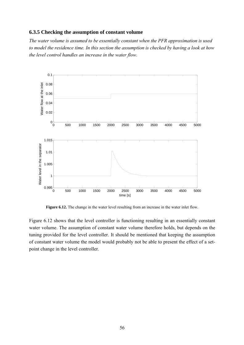
56

6.3.5 Checking the assumption of constant volume The water volume is assumed to be essentially constant when the PFR approximation is used to model the residence time. In this section the assumption is checked by having a look at how the level control handles an increase in the water flow.

0 500 1000 1500 2000 2500 3000 3500 4000 4500 50000

0.02

0.04

0.06

0.08

0.1

Wat

er fl

ow a

t the

inle

t

0 500 1000 1500 2000 2500 3000 3500 4000 4500 50000.995

1

1.005

1.01

1.015

time [s]

Wat

er le

vel i

n th

e se

para

tor

Figure 6.12. The change in the water level resulting from an increase in the water inlet flow.

Figure 6.12 shows that the level controller is functioning resulting in an essentially constant water volume. The assumption of constant water volume therefore holds, but depends on the tuning provided for the level controller. It should be mentioned that keeping the assumption of constant water volume the model would probably not be able to present the effect of a set-point change in the level controller.

57

7. Modelling the hydrocyclone This chapter presents the modelling of a static hydrocyclone. As a result of the complexity of hydrocyclone operation due to the two folded vortex structure and the effect of drop composition, prior modelling is found based either on very simple empirical relationships or on complex structures using computational fluid dynamics.

Energy balances have been neglected and Simulink used for the modelling based on the assumptions presented in chapter 6, on modelling the separator.

The accuracy level wanted for the hydrocyclone is the same as for the separator sufficient for use in process control purposes.

7.1 The main assumptions In modelling simplifications are always introduced. The extent of the simplification depends on the accuracy level wanted for the model. In this section a presentation is provided of the main assumptions made modelling a static hydrocyclone. In contrast to the separator the hydrocyclone was modelled as a static unit. The residence time of seconds support this choice [24].

7.1.1 Transforming and using the Rietema equations in oil from water separation The hydrocyclone equations described by Rietema for a solid from liquid separation are assumed to be valid also for the de-oiling hydrocyclone based on the assumptions stated in this section and taking into consideration the wanted accuracy level for the model. Equations 5.2 and 5.3 presented by Rietema provide a measure of the cut size depending on the inflow and pressure drop. The equations were originally provided for a hydrocyclone separating out solids dispersed in a liquid. Based on the assumption that any hydrocyclone separating particles (solid, droplets or gas bubbles) of the dispersed phase from a continuous liquid is separating on the basis of the density difference between the phases [25], the equations were for of the hydrocylone separation of oil from water, after having made some adjustments.

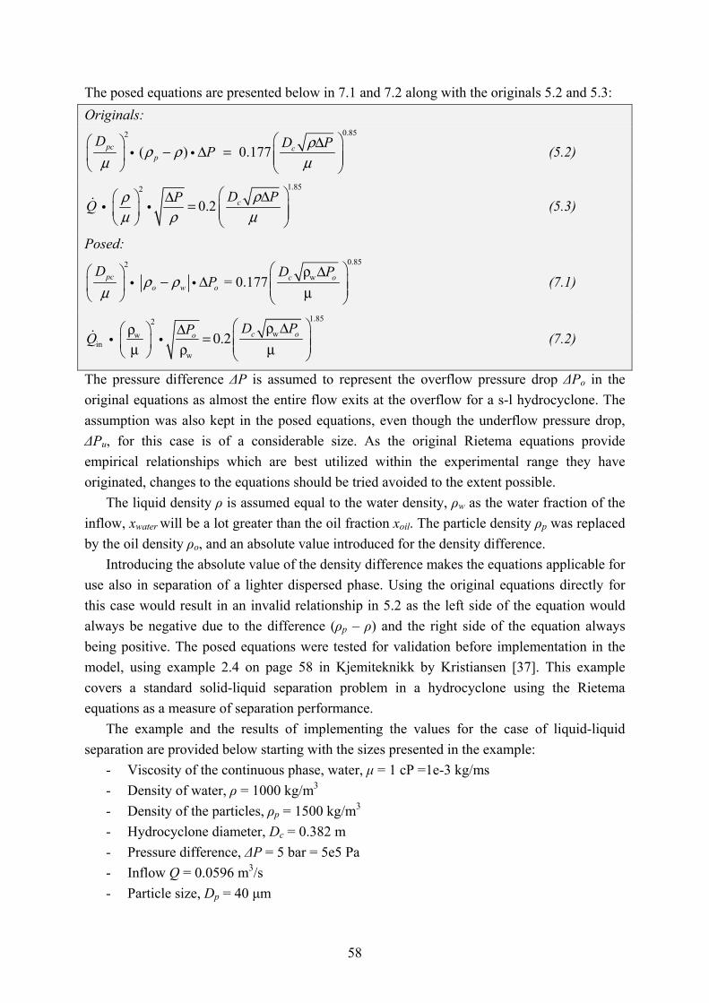
58

The posed equations are presented below in 7.1 and 7.2 along with the originals 5.2 and 5.3: Originals:

0.852

( ) 0.177pc cp

D D PP

ρρ ρμ μ

⎛ ⎞⎛ ⎞ Δ − Δ = ⎜ ⎟⎜ ⎟ ⎜ ⎟⎝ ⎠ ⎝ ⎠

i i (5.2)

1.852

0.2 cD PPQρρ

μ ρ μ⎛ ⎞Δ⎛ ⎞ Δ = ⎜ ⎟⎜ ⎟ ⎜ ⎟⎝ ⎠ ⎝ ⎠

i i (5.3)

Posed: 0.852

w = 0.177pc c oo w o

D D PPρ ρ

μ⎛ ⎞ρ Δ⎛ ⎞

− Δ ⎜ ⎟⎜ ⎟ ⎜ ⎟μ⎝ ⎠ ⎝ ⎠i i (7.1)

1.852ww

inw

c oo D PPQ⎛ ⎞ρ Δ⎛ ρ ⎞ Δ = 0.2⎜ ⎟⎜ ⎟ ⎜ ⎟μ ρ μ⎝ ⎠ ⎝ ⎠

i i (7.2)

The pressure difference ΔP is assumed to represent the overflow pressure drop ΔPo in the original equations as almost the entire flow exits at the overflow for a s-l hydrocyclone. The assumption was also kept in the posed equations, even though the underflow pressure drop, ΔPu, for this case is of a considerable size. As the original Rietema equations provide empirical relationships which are best utilized within the experimental range they have originated, changes to the equations should be tried avoided to the extent possible.

The liquid density ρ is assumed equal to the water density, ρw as the water fraction of the inflow, xwater will be a lot greater than the oil fraction xoil. The particle density ρp was replaced by the oil density ρo, and an absolute value introduced for the density difference.

Introducing the absolute value of the density difference makes the equations applicable for use also in separation of a lighter dispersed phase. Using the original equations directly for this case would result in an invalid relationship in 5.2 as the left side of the equation would always be negative due to the difference (ρp – ρ) and the right side of the equation always being positive. The posed equations were tested for validation before implementation in the model, using example 2.4 on page 58 in Kjemiteknikk by Kristiansen [37]. This example covers a standard solid-liquid separation problem in a hydrocyclone using the Rietema equations as a measure of separation performance.

The example and the results of implementing the values for the case of liquid-liquid separation are provided below starting with the sizes presented in the example:

- Viscosity of the continuous phase, water, μ = 1 cP =1e-3 kg/ms - Density of water, ρ = 1000 kg/m3 - Density of the particles, ρp = 1500 kg/m3 - Hydrocyclone diameter, Dc = 0.382 m - Pressure difference, ΔP = 5 bar = 5e5 Pa - Inflow Q = 0.0596 m3/s - Particle size, Dp = 40 μm

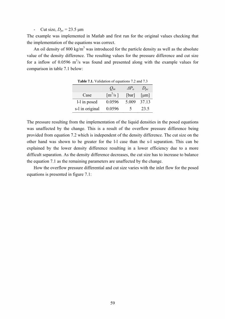
59

- Cut size, Dpc = 23.5 μm The example was implemented in Matlab and first run for the original values checking that the implementation of the equations was correct.

An oil density of 800 kg/m3 was introduced for the particle density as well as the absolute value of the density difference. The resulting values for the pressure difference and cut size for a inflow of 0.0596 m3/s was found and presented along with the example values for comparison in table 7.1 below:

Table 7.1. Validation of equations 7.2 and 7.3

Qin ΔPo Dpc Case [m3/s ] [bar] [μm]

l-l in posed 0.0596 5.009 37.13 s-l in original 0.0596 5 23.5

The pressure resulting from the implementation of the liquid densities in the posed equations was unaffected by the change. This is a result of the overflow pressure difference being provided from equation 7.2 which is independent of the density difference. The cut size on the other hand was shown to be greater for the l-l case than the s-l separation. This can be explained by the lower density difference resulting in a lower efficiency due to a more difficult separation. As the density difference decreases, the cut size has to increase to balance the equation 7.1 as the remaining parameters are unaffected by the change.

How the overflow pressure differential and cut size varies with the inlet flow for the posed equations is presented in figure 7.1:

60

0 0.02 0.04 0.06 0.08 0.1 0.12 0.14 0.16 0.18 0.20

1

2

3

4

5

6

7

8

9

Qin

Δ Po

Dpc

Figure 7.1. The cut size and overflow pressure differential resulting from the posed equations 7.1 and 7.2.

From figure 7.1 it is shown that as the inlet flow rate, Qin, increases, the overflow pressure

difference ΔPo = Pin – Poverflow increases as a result of Pin increasing. The increase in the inlet flow will provide a faster movement of the fluids inside the hydrocyclone resulting in a more efficient gravitation and a decrease in Dpc.

The order of magnitude of the pressure drop and the cut size resulting from the posed equations for the case of l-l separation seems to be correct and the relationships are reacting as expected to changes in flow.

Lydersen in [39] rapports that for larger hydrocyclones, agreement between calculations according to Rietema and experimental results have been reported also for liquid-liquid operation, while the efficiency of a smaller cyclone was reported to be poorer due to disintegration of drops within the cyclone. Keeping the relative dimensions recommended by Rietema, the results from the model should represent the effect of operation sufficiently.

The dimensions provided in the example 2.4 presented by Kristiansen [37] were kept in the model on the assumption of the example being adjusted to work well within the application range of the equations, again stressing the empirical nature of the equations.

61

The geometrical relationships of a hydrocyclone recommended by Rietema and provided with the original equations are shown in the figure 5.3. The dimension of a light dispersion hydrocyclone would normally be longer. Roald [35] argues that the length of a liquid – liquid hydrocyclone is 10-12 times the cyclone diameter, Dc , which is at least twice the length of the one provided by Rietema of 5 times Dc. That the hydrocyclone structure coinciding with the equations probably is too short compared to the l-l hydrocyclone dimensions found on oil-rigs may result in a larger cut size than what is actually the case resulting from model simulations.

Rietema recommended operation with approximately 10% of the liquid leaving as underflow and 90% as overflow [39]. For most de-oiling hydrocyclones, the overflow rate, Qoverflow, is only a few percent of the inlet flow rate, Qinlet, (<10 [23]) [11]. Still on some installations hydrocyclones are found de-watering oil downstream from the production separator [2], where the main flow will be overflow as for the Rietema equations. The density difference seems to be the most important factor.

The performance criteria affecting the operation of a hydrocyclone presented in section 5.2 shows that the optimum operation of the inlet flow rate to a hydrocyclone is within a range. It can be argued that introducing a safety margin making sure that the flow rate stays within the optimal range and does not vary significantly, hence providing an approximately constant flow split; it may balance of the deviations resulting from the prior assumptions made in this section.

7.1.2 Coalescence and drop breakup Svarovsky [25] states that the separation in hydrocyclones depends highly on particle size or particle density if the system is not homogeneous, as for the case of immiscible liquids. The compartment representation for the drop size effect made out during the separator modelling in section 6.2.2 is maintained for the hydrocyclone providing a measure of the drop size effect on performance. Including the effect also provides consistency to the model.

Introducing the effect of coalescence was tried but found difficult for the static hydrocyclone, because coalescence has a direct effect on hydrocyclone performance. Implementing the effect of coalescence before the estimation of efficiency would result in a too high estimated performance, whereas the opposite would be true for subsequent implementation. As a result the effect of coalescence was excluded from the hydrocyclone model. Drop size characterization is in general difficult for hydrocyclones as a result of the droplets being subjected to excessive shear forces during sampling and coalescence afterwards. Hence, checking the effect to real data if it was to be left implemented would be difficult.

The presence of turbulence can provoke drop breakup in the hydrocyclone, a tendency which should be tried avoided as best possible [45]. In the model the effect of drop breakup is assumed to be negligible on the basis of the results provided by Thew in [23] which states that no oil drop breakup occurred detrimental to separation performance. That oil-dispersions

62

where the mean drop size is already very small (< 50μm) are less susceptible to further reduction in size as a result of the high shear rate was also taken into consideration providing the assumption [2].

7.1.3 Liners A hydrocyclone unit usually houses more than one liner. The liner configuration of hydrocyclones was presented in section 5.1. Ideally the number of liners corresponds to the desired output per liner [23], and is in the model implemented to have the opportunity of increasing the capacity with increased inflow. Hence a too large pressure drop over the hydrocyclone is avoided and the model is kept within its operating range.

7.1.4 Bernoulli’s equation providing the flow through the hydrocyclone Bernoulli’s equation can be used to describe the flow from the inlet to the underflow outlet in the hydrocyclone. An assumption of Bernoulli’s equation being sufficient in presenting the flow from the inlet to the underflow outlet was made. The general equation is stated as,

2 2

2 2in in u u

in uin u

v P v Pgh ghρ ρ

+ + = + + (7.3)

where g is the gravity constant, hin and hu is the height-, vin and vu is the speed of the fluid- and Pin and Pu the pressures at the inlet and underflow respectively. ρin is the inlet density and ρu is the density of the underflow which are provided knowing the oil and water densities as well as the fractions of oil xoil_in and xoil_u and water xwater_in and xwater_u at the respective outlets. These densities are:

_ _ ( ) ( )in oil in oil water in waterx xρ ρ ρ= +i i (7.4)

_ _ ( ) ( )u oil u oil water u waterx xρ ρ ρ= +i i (7.5)

The hydrocyclone is assumed to be placed horizontally which is the orientation most commonly found on an oil-rig. As a result of the positioning the average height the fluid travels is assumed to be from the inlet to the centre of the inner vortex, which is further assumed to align with the coordinate x-axis, see figure 7.2. Hence the height of the underflow equals zero height. The height of the inlet is assumed equal to half a cyclone diameter in accordance with the geometrical dimensions presented for the Rietema equations in figure 5.3.

The speeds at the inlet and underflow are estimated knowing the fluid flows at the respective outlets and providing a measure for the belonging areas where the fluid enters and

63

leaves. The pressure drop inside the hydrocyclone is assumed significantly grater than the one the fluid experiences inside the pipes and entering, and as a result the inlet diameter is assumed equal to the cyclone diameter. The speed of the fluid out of the hydrocyclone is a lot higher than the speed entering as a result of the underflow diameter being a lot smaller than the hydrocyclone diameter. A speed correction factor, SCunderflow is introduced for the underflow area to compensate for this effect assuming that the diameter of the underflow is equal to the cyclone diameter divided by the factor. SCunderflow works as a tuning parameter and has to be adjusted before running model simulations. For a given set of data this is done by first running the model to find the initial underflow pressure loss, and then adjusting the speed correction factor until the pressure drop operates in an approved range. The number of liners used for the case also needs to be taken into consideration as the pressure drop will be distributed over the liners.

Figure 7.2. The assumption of Bernoulli’s equation for the flow from the inlet

to the underflow outlet of a hydrocyclone Rewriting the velocities we get:

( )

22

22

4 4 /

2 2

uin

c underflowc in uin

in u

QQD SCD P Pgh

ππρ ρ

⎛ ⎞⎛ ⎞ ⎜ ⎟⎜ ⎟ ⎜ ⎟⎝ ⎠ ⎝ ⎠+ + = + (7.6)

where Qin and Qu are the flows at the inlet and underflow respectively, Dc is the cyclone diameter and SCunderflow is the speed correction factor.

As long as the horizontal arrangement is used the fact that the length of a light dispersion hydrocyclone probably is longer is not included. The fact is that the hydrocyclone should probably have been narrower as well as a result of the same design argumentation used in 7.1.1. Using a vertical hydrocyclone the increased length could have been taken into consideration in the Bernoulli equation as it is not included in the Rietema equations and therefore would not affect the quality of using the empirical relationships they provide.

64

7.1.5 The effect of separation The hydrocyclone performance is provided as a combination of three effects. The drop size of the oil drops going in, the inlet flow and the flow split. Combining the Rietema equations 5.2 and 5.3 it is seen that the cut size is given as long as the inflow is provided. The efficiency is provided as a relationship depending on the drop size as well as the inflow presenting it as a function of the particle size ratio k = Dp/Dpc. This dependence is shown in figure 7.3, where the efficiency is given depending on k as presented in equation 7.7.

0, 0.4 1.25 k - 0.75, 0.4 1.6

1, 1.6

kk

kη

<⎧⎪= ≤ ≤⎨⎪ >⎩

i (7.7)

The relationship between the efficiency and the particle size ratio presented in figure 7.3 is based on the one experimentally determined by Rietema and belonging to the equations as presented by Lydersen in [39]. The relationship is based on the size of a drop compared to the cut size and it is seen from figure 7.3 that the efficiency equals 0.5 when the particle size equals the cut size. Using Rietema’s relationship providing the efficiency from the particle size ratio zero performance is assumed to occur for k below 0.4, that is for particles 60% below the cut size and complete separation is assumed for particles 60% above the cut size, see equation 7.7.

The slope of the curve predicting the separation performance going from zero to complete separation is referred to as the sharpness of cut and is an important factor in assessing hydrocyclone performance as it controls the amount of misplaced material in the two products. The cut is commonly found quite sharp for hydrocyclones and sharpness increases proportionally to the density difference between the fluids to be separated [23]. As the relationship is made out for a greater density difference than the one it is used for in this case the cut provided in the model might be a bit sharper than what is actually the case for l-l separation. The sharpness can be adjusted by using several hydrocyclones in parallel.

65

Figure 7.3. The efficiency dependence on the particle size ratio.

The shape presented by the curve in figure 7.3 is referred to as the typical ‘separation

curve’ by Delfos in [46]. Providing a description of the range of drop sizes, in which the separation efficiency falls from close to one to close to zero. As stated in section 7.1.2 the compartment presentation was provided also for the hydrocyclone having the same mean drops sizes presented in table 6.1. Since the cut in the hydrocyclone is quite sharp the cut will most likely affect only one or two compartments. Hence, for the remaining compartments all of the oil droplets will either be separated out or remain dispersed in the water and exit through the underflow, see equation 7.7. This effect is illustrated in figure 7.4 below, which also shows that as the flow rate increases or decreases the cut will move its position within the compartments. An increase in Qin will result in a decrease in the cut size and a movement of the cut to the left in figure 7.4 including compartments with smaller mean drop sizes.

Figure 7.4. The compartments affected by the cut depending on the inflow size.

66

As a result of the Rietema equations 5.2 and 5.3 providing the cut size originating from s-l separation there is no effect of the flow split on the efficiency. This is not surprising as almost the entire inflow will exit in the overflow for the s-l case. Introducing an additional effect of the flow split defined in equation 5.4 is necessary in the case of l-l separation taking into consideration that for very small values of Qo the performance will be poor despite of a small Dpc which only depends on the inflow.

An issue with using the dependence on cut size to provide the separation performance is that the amount of oil estimated to in the over- or underflow in theory may be larger than the total over- or underflow respectively. This is a result of the estimation of the oil fractions depending only on the water inlet flow in addition to the oil fraction at the inlet and not including the distribution of the flows going out of the two outlets. Limitations had to be introduced to handle the effect and were provided for the under- and overflow oil estimations so that they could not be larger than the total flows. When this effect takes place, the model is probably outside its area of application and operation in this area over an extended time may imply that the model becomes inapplicable.

The efficiency dependence on flow split is introduced using the data provided by Medrum [24] and illustrated by Husveg [8] in the figure 5.5 which has been edited to get a clearer image of the data represented below in figure 7.5:

Figure 7.5. Two alternatives for the efficiency dependency on flow split considered implemented in the model.

Two alternatives were considered, the sharper route to maximum efficiency b) and a) having a slower rise. The more conservative route a) was chosen to compensate for the assumptions made using the solid-liquid Rietema equations for the liquid-liquid separation as presented at the start of the chapter.

The effect of the flow split is given as,

0.595 FS FSη = i (7.8)

and is introduced as a limitation to the hydrocyclone performance after the over and underflows have been estimated. If at this point the flow split is less than 1.53% the total separation efficiency is reduced to what is provided by equation 7.8. As long as the FS is

67

above 1.53% optimal efficiency is provided, but is limited to ηFS = 91% representing the maximum in figure 7.5. The limitation of the efficiency to a maximum value of 91 % is in accordance with both the figures 5.4 and 5.5 providing the efficiency relationship to flow rate and flow split respectively presented by Meldrum [24] and provided again by Husveg [8, 11]. The limitation to the maximum efficiency is also thought as a measure providing a conservative rather than an optimistic model presentation as a way of compensating for the previously mentioned assumptions.

The total flows of oil exiting over and underflow of the hydrocyclone is provided by the relationships presented in 7.9 and 7.10

_ _ _oil o tot FS oil oQ Qη = i (7.9)

_ _ _ _(1 )oil u tot oil u FS oil oQ Q Qη = + − i (7.10)

The optimal hydrocyclone inflow is found within a range as discussed in section 5.2 concerning hydrocyclone performance criteria. What corresponds to the minimum and maximum flows limiting this range depends on the hydrocyclone design as well as the flow size and composition for which it is used. The minimum flow split criteria was provided for the model using the relationship provided by Meldrum. The flow split is provided as a relationship between two flows as presented in equation 5.4, and is independent of the size of the flows as a result. Limitations providing the optimum flow rate range should be implemented, but approximations of the limits are best provided using data for the case to be studied by the model. The limits introduced should exclude flow rates that have proven to affect hydrocyclone performance negatively, and a narrower optimal range of operation is recommended.

7.2 Mass balances In addition to the equations resulting from the assumptions presented in 7.1 mass balances provide additional information necessary to complete the model repressentation.

Figure 7.6. The in and outlets of the hydrocyclone

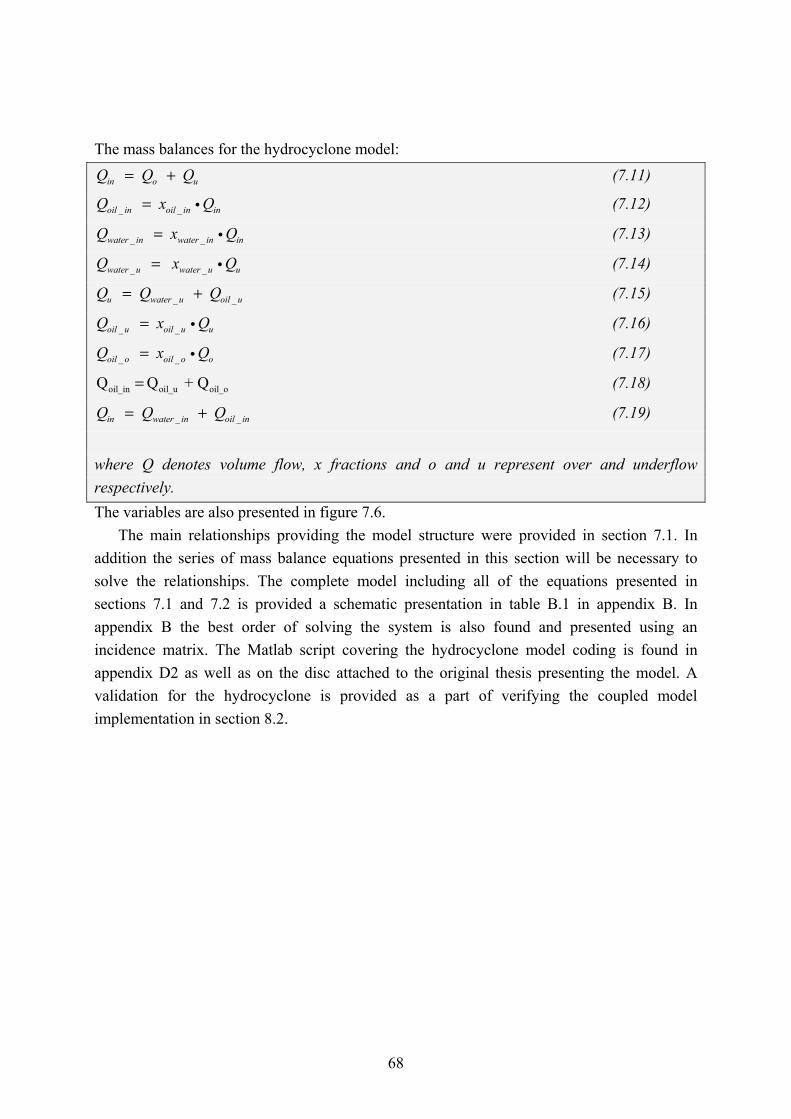
68

The mass balances for the hydrocyclone model:

in o uQ Q Q= + (7.11)

_ _ oil in oil in inQ x Q= i (7.12)

_ _ water in water in inQ x Q= i (7.13)

_ _ water u water u uQ x Q= i (7.14)

_ _ u water u oil uQ Q Q= + (7.15)

_ _ oil u oil u uQ x Q= i (7.16)

_ _ oil o oil o oQ x Q= i (7.17)

oil_in oil_u oil_oQ Q + Q = (7.18)

_ _ in water in oil inQ Q Q= + (7.19)

where Q denotes volume flow, x fractions and o and u represent over and underflow respectively. The variables are also presented in figure 7.6.

The main relationships providing the model structure were provided in section 7.1. In addition the series of mass balance equations presented in this section will be necessary to solve the relationships. The complete model including all of the equations presented in sections 7.1 and 7.2 is provided a schematic presentation in table B.1 in appendix B. In appendix B the best order of solving the system is also found and presented using an incidence matrix. The Matlab script covering the hydrocyclone model coding is found in appendix D2 as well as on the disc attached to the original thesis presenting the model. A validation for the hydrocyclone is provided as a part of verifying the coupled model implementation in section 8.2.

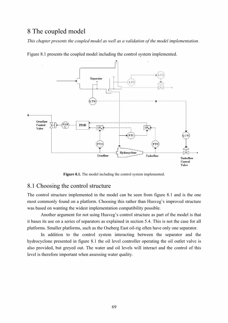
69

8 The coupled model This chapter presents the coupled model as well as a validation of the model implementation. Figure 8.1 presents the coupled model including the control system implemented.

Figure 8.1. The model including the control system implemented.

8.1 Choosing the control structure The control structure implemented in the model can be seen from figure 8.1 and is the one most commonly found on a platform. Choosing this rather than Husveg’s improved structure was based on wanting the widest implementation compatibility possible. Another argument for not using Husveg’s control structure as part of the model is that it bases its use on a series of separators as explained in section 5.4. This is not the case for all platforms. Smaller platforms, such as the Oseberg East oil-rig often have only one separator.

In addition to the control system interacting between the separator and the hydrocyclone presented in figure 8.1 the oil level controller operating the oil outlet valve is also provided, but greyed out. The water and oil levels will interact and the control of this level is therefore important when assessing water quality.

70

8.2 Validation of the coupled model While model validation on a dynamic level should check that the model is able to properly predict the transient behaviour of the system, validation on a static level should check that the model correctly predicts the steady-state conditions [4].

In this section three different cases will be provided to verify the implementation of the coupled model.

1) Changing the water inlet flow to the separatort. 2) Changing the number of droplets entering. 3) Changing the mean drop sizes of the compartments.

The implementation of the separation cut provided by the hydrocyclone is also provided a short discussion. There are three main results presenting separation performance in the model.

a) The oil fraction exiting with the separator water outlet presenting the separation performance of the separator as well as the hydrocyclone workload.

b) The oil fraction separated out of the hydrocyclone presenting hydrocyclone separation performance.

c) The oil fraction still dispersed at the hydrocyclone water outlet providing a measure of the water purity obtained by the water treatment plant.

The separator was provided a validation after the modelling was complete and the results presented in section 6.3. This first stage validation was done to make sure that the dynamic unit was functioning properly before the hydrocyclone was included in the system. The implementation of the hydrocyclone model will be validated as part of the coupled model in this section. Hence the main focus of this validation will be on how the hydrocyclone reacts to the changes presented above, but at the same time the interaction with the separator will be taken into account.

71

8.2.1 Changing the water inlet Increasing the water flow at the separator inlet expecting the overall performance of the model to be provided as the result of a weighing of the effect of a decrease in separation performance for the separator to the effect of an increase in hydrocyclone performance.

1300 1350 1400 1450 1500 1550 1600 1650 1700

0.9

1

1.1

1.2

1.3

x 10-5

Oil

fract

ion

still

dis

pers

edat

the

sepa

rato

r wat

er o

utle

t

1300 1350 1400 1450 1500 1550 1600 1650 17000

0.5

1

1.5

2x 10-5

Oil

fract

ion

sepa

rate

dou

t of t

he h

ydro

cycl

one

1300 1350 1400 1450 1500 1550 1600 1650 17004

6

8

10

12x 10-6

time [s]

Oil

fract

ion

still

dis

pers

ed

at th

e hy

droc

yclo

ne w

ater

out

let

1300 1350 1400 1450 1500 1550 1600 1650 17000.04

0.05

0.06

0.07

Wat

er fl

ow a

t the

sepa

rato

r inl

et

Figure 8.2. The change in separation performance, resulting from an increase in separator water inlet flow.

Figure 8.2 shows the expected decrease in performance for the separator resulting in a higher oil fraction in the water flow entering the hydrocyclone.

72

For the hydrocyclone the dependence of the cut size, dpc, on the overflow pressure drop, ΔPo, and the pressure drop’s succeeding dependence on the water inlet flow, Qin, from the equations 7.1 and 7.2 are provided below in the relationships 8.1 and 8.2:

0.575

1pc

o

DP

⎛ ⎞∝ ⎜ ⎟⎜ ⎟Δ⎝ ⎠

(8.1)

( )0.425o inP QΔ ∝ (8.2)

As the flow increases so does the overflow pressure drop according to relationship 8.2. A decrease in the cut size will follow as a result of the increased pressure difference as seen from the relationship 8.1. Performance is expected to increase, and this is what is seen from figure 8.2.

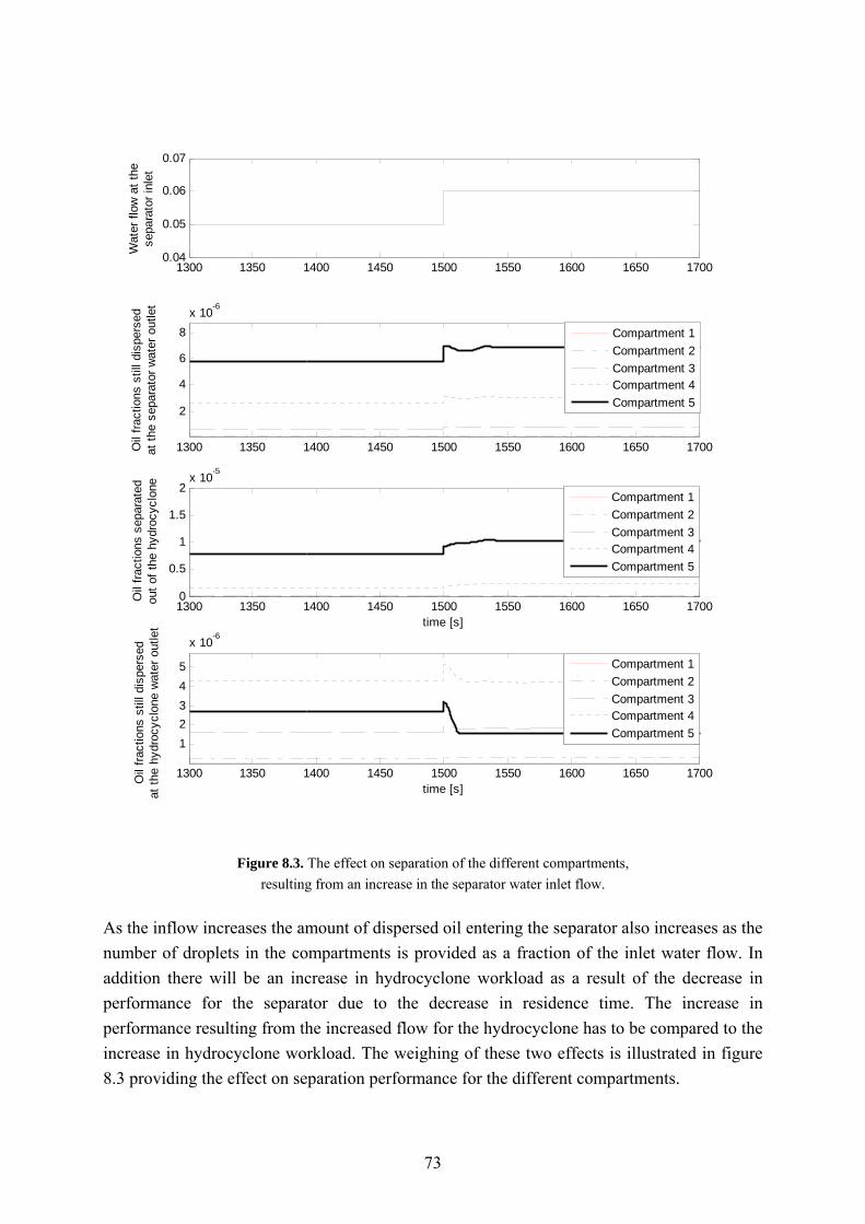
73

1300 1350 1400 1450 1500 1550 1600 1650 1700

2

4

6

8x 10-6

Oil

fract

ions

stil

l dis

pers

edat

the

sepa

rato

r wat

er o

utle

t

1300 1350 1400 1450 1500 1550 1600 1650 17000

0.5

1

1.5

2x 10-5

time [s]

Oil

fract

ions

sep

arat

edou

t of t

he h

ydro

cycl

one

1300 1350 1400 1450 1500 1550 1600 1650 1700

12345

x 10-6

time [s]

Oil

fract

ions

stil

l dis

pers

edat

the

hydr

ocyc

lone

wat

er o

utle

t

1300 1350 1400 1450 1500 1550 1600 1650 17000.04

0.05

0.06

0.07

Wat

er fl

ow a

t the

sepa

rato

r inl

et

Compartment 1Compartment 2Compartment 3Compartment 4Compartment 5

Compartment 1Compartment 2Compartment 3Compartment 4Compartment 5

Compartment 1Compartment 2Compartment 3Compartment 4Compartment 5

Figure 8.3. The effect on separation of the different compartments, resulting from an increase in the separator water inlet flow.

As the inflow increases the amount of dispersed oil entering the separator also increases as the number of droplets in the compartments is provided as a fraction of the inlet water flow. In addition there will be an increase in hydrocyclone workload as a result of the decrease in performance for the separator due to the decrease in residence time. The increase in performance resulting from the increased flow for the hydrocyclone has to be compared to the increase in hydrocyclone workload. The weighing of these two effects is illustrated in figure 8.3 providing the effect on separation performance for the different compartments.

74

For compartment 5 the effect of the increase in performance is shown to exceed the increase of contamination as more oil is separated out, presented as a decrease in the oil fraction still dispersed at the underflow outlet in addition to the increased oil fraction exiting with the overflow. Compartment 4 also shows an increased performance as a result of the increased inflow, but the oil fraction still dispersed at the water outlet is approximately unchanged. Hence the increase in performance was not enough to overcome the increase in contamination. For compartment 3 the increase in contamination exceeds the increase in performance. Compartments 1 and 2 still have mean droplet diameters too small compared to the cut size to be separated resulting in an increase in the oil fractions still dispersed at the hydrocyclone water outlet.

The model performed satisfactory to a change in inlet flow.

75

8.2.2 Changing the drop composition at the inlet Increasing the number of large droplets entering the separator as it is an interesting aspect of succeeding model application and a disturbance the model should be able to handle.

1300 1350 1400 1450 1500 1550 1600 1650 1700

0.075

0.08

0.085

Oil

fract

ion

in c

ompa

rtmen

t 5en

terin

g th

e se

para

tor

1300 1350 1400 1450 1500 1550 1600 1650 1700

0.91

1.11.2

1.3

x 10-5

Oil

fract

ion

still

dis

pers

ed

at th

e se

para

tor w

ater

out

let

1300 1350 1400 1450 1500 1550 1600 1650 17000

0.5

1

1.5

2x 10-5

Oil

fract

ion

sepa

rate

dou

t of t

he h

ydro

cycl

one

1300 1350 1400 1450 1500 1550 1600 1650 17004

6

8

10

12x 10-6

time [s]

Oil

fract

ions

stil

l dis

pers

edat

the

hydr

ocyc

lone

wat

er o

utle

t

Figure 8.4. The effect on separation resulting from an increase in the number of the largest droplets.

Figure 8.4 shows that an increase in the number of the largest drops increases the oil fraction entering the hydrocyclone from the separator. The oil fraction separated out of the hydrocyclone increases but there is also a decrease in the water purity provided by the system.

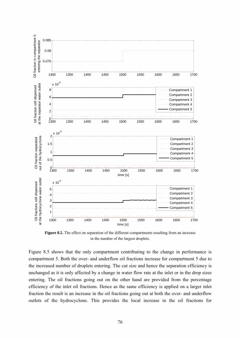
76

1300 1350 1400 1450 1500 1550 1600 1650 1700

0.075

0.08

0.085

Oil

fract

ion

in c

ompa

rtmen

t 5en

terin

g th

e se

para

tor

1300 1350 1400 1450 1500 1550 1600 1650 17000

2

4

6

8x 10-6

Oil

fract

ion

still

dis

pers

ed

at th

e se

para

tor w

ater

out

let

Compartment 1Compartment 2Compartment 3Compartment 4Compartment 5

1300 1350 1400 1450 1500 1550 1600 1650 17000

0.5

1

1.5

2x 10-5

time [s]

Oil

fract

ion

sepa

rate

dou

t of t

he h

ydro

cycl

one

Compartment 1Compartment 2Compartment 3Compartment 4Compartment 5

1300 1350 1400 1450 1500 1550 1600 1650 1700

1

2

3

4

5

x 10-6

time [s]

Oil

fract

ions

stil

l dis

pers

edat

the

hydr

ocyc

lone

wat

er o

utle

t

Compartment 1Compartment 2Compartment 3Compartment 4Compartment 5

Figure 8.5. The effect on separation of the different compartments resulting from an increase

in the number of the largest droplets. Figure 8.5 shows that the only compartment contributing to the change in performance is compartment 5. Both the over- and underflow oil fractions increase for compartment 5 due to the increased number of droplets entering. The cut size and hence the separation efficiency is unchanged as it is only affected by a change in water flow rate at the inlet or in the drop sizes entering. The oil fractions going out on the other hand are provided from the percentage efficiency of the inlet oil fractions. Hence as the same efficiency is applied on a larger inlet fraction the result is an increase in the oil fractions going out at both the over- and underflow outlets of the hydrocyclone. This provides the local increase in the oil fractions for

77

compartment 5 while the oil fractions going out of the other compartments remain unaffected by the change.

The model responded satisfactory to the disturbance.

8.2.3 Changing the mean drop sizes of the compartments Decreasing the mean drop sizes of the compartments expecting poorer separation. The mean drop size for each compartment was decreased by 50% in the model. The values representing the change in drop sizes are presented in table 8.1, and the effect of the changes on the separation in table 8.2.

Table 8.1. The initial and final values of the drop sizes. Dp

[μm] Compartment 1 Compartment 2 Compartment 3 Compartment 4 Compartment 5

Initial 5 15 30 60 100 Final 2.5 7.5 15 30 50

Table 8.2. The effect of decreasing the dispersed drop sizes entering the model.

Oil fraction still dispersed at

the separator water outlet Oil fraction separated out

of the hydrocyclone Oil fraction still dispersed at

the hydrocyclone water outlet

Initial Final Initial Final Initial Final

[10-6] [10-6]

Change [%]

[10-6] [10-6]

Change [%]

[10-6] [10-6]

Change[%]

Compartment 1

0.02595 0.02597 0.07707 0 0 0 0.06838 0.06838 0

Compartment 2

0.10379 0.10387 0.07708 0 0 0 0.27351 0.27354 0.01097

Compartment 3

0.64854 0.64905 0.07835 0.3657 0 - 100 1.6494 1.7220 4.402

Compartment 4

2.5937 2.5935 0.2274 1.560 0.1463 - 90.61 4.2817 6.5948 54.02

Compartment 5

5.8174 5.8306 0.2613 7.729 2.450 - 68.30 2.6919 11.36 322.0

Total 9.1894 9.203 0.1480 9.655 2.596 - 73.11 8.964 20.02 123.3 Table 8.2 show a poorer separation in the separator as well as in the hydrocyclone as expected. The effect of the decrease in the mean drop sizes in the compartments is greater for

78

the hydrocyclone as it affects the efficiency directly whereas it only provides a minimum value for the separator efficiency.

The cut in the hydrocyclone has moved as a result of the decreased drop sizes and the oil drops in compartment 3 are now too small to get separated, see figure 7.4. k = Dp/Dpc

decreases with the decreasing drop sizes and more oil goes out through the underflow. With regards to the performance the drop size is compared to the cut size which is unchanged as the inlet flow is constant. The compartments experiencing separation initially must all have had a drop size above 60% of the cut size, see figure 7.3. The decrease in drop sizes results in the size of the droplets in compartment 3 becoming smaller than the limit of 60% of Dpc providing separation. The drop sizes of compartments 4 and 5 are also at a lesser percentage of the cut size for the final value. As compartment 5 goes from having the largest oil fraction exiting overflow initially to the largest fraction found underflow after the decrease it has a mean drop size going from initially being larger than the cut size to becoming smaller. The compartment 4 mean drop size is smaller than the cut size in both cases as the larger oil fraction is found in the underflow both before and after the change.

The model performed satisfactory to a change in the mean droplet sizes in the compartments.

8.2.4 The hydrocyclone cut Checking to see if the hydrocyclone cut functions properly. Giving the values presented for the final efficiency in table 8.2 a closer look it is seen that the cut in the hydrocyclone is provided in the compartments 4 and 5 as fractions of these compartments are present at both the overflow- and the underflow exit. The mean drop sizes in the compartments 1-3 are all too small to undergo separation. The fraction of oil leaving with the underflow compared to the fraction leaving with the overflow is greater for compartment 4 than for compartment 5 as expected

The cut seems to function properly.

79

9. Conclusion The main environmental impacts from an offshore oil-rig are pollutive gases emitted to the air, hazardous chemicals utilized in production, and oil dispersed in the water discharged to sea. Further, an offshore oil-rig consumes large amounts of energy, which leads to indirect environmental impacts if this energy is not renewable.

Several water purification alternatives exist to remove dispersed oil, and in the offshore industry over 90% are based on hydrocyclone technology.

Due to the complex nature of the two-phase flow and the variance in the drop sizes of the dispersed phase it is difficult to model oil and water separation. In the literature a spectre of models from purely empirical to very complex models can be found. In this study a water purification model is provided combining a dynamic separator with a static hydrocyclone, as this configuration is often found in the industry. The model is made for use in process control purposes and includes an integrated control system.

The separator efficiency is based on the residence time as well as an additional effect of drop size. The residence time dependence was provided using a plug flow reactor approximation for the fluid flow, and presenting the variance in oil concentration with time as a second order function. An increase in the residence time or increased drop sizes entering the separator increases performance.

The hydrocyclone model performance depends on fluid inflow and drop composition. The optimal inflow should be held within a given range and the flow split maintained above a certain level.

A validation of the modelling has been done, and the results seem reasonable.

80

10. Suggestions to further work In this section some suggestions for future work to further improve the model will be provided. In the work presented in this thesis a water purification model was provided and the model implementation validated. Some ideas for further work on the model are listed below: - Validation of the model using data: The model implementation has been verified, but

validation in comparison to physical or experimental data still remains, and should be done before the model is put to use. We hope that the model is generic to an extent that fitting the model to experimental data can be performed within a reasonable amount of time.

- Introducing the optimal operating flow range: When data representing the model flow is available the optimal flow range should be found and implemented.

- Putting the model to use: The model should be able to run simulations to study the effect of changes in the tuning parameters. Running various cases a tuning strategy to minimize the environmental impact is hoped to culminate.

- Expand the model: The model can be expanded to include for example the effect of chemicals on separation performance. Additional equipment, such as coalescers, can also be modelled and added to the model when it is present in the system to be studied providing an even closer resemblance.

- Coupling the water treatment model to the already existing model of the oil- and gas-train: Coupling the water treatment model with the already existing model of the oil and gas train a model of a complete oil-platform results providing a measure of the overall environmental impact of an offshore processing plant. The complete platform model would be especially useful for studying the effect the different stages of production have on each other. The models will have to be scaled to fit each other prior to the coupling.

81

Bibliography 1. Pettersen, T., Tuning and Control Strategy for an Offshore Process Subject to

Minimum Environmental Impact, in Chemical Engineering. 2007, NTNU: Trondheim. 2. A. Belaidi and Thew, M.T., The Effect of Oil and Gas Content on the Controllability

and Separation in a De-Oiling Hydrocyclone. Chemical Engineering Research and Design, 2003. 81(3): p. 305-314.

3. Choi, M.S., Hydrocyclone Produced Water Treatment for Offshore Developments. In:

Paper SPE 20662 Presented at the Annual Technical Conference and Exhibition, New Orleans, Louisiana, 23-26 September, 1990: p. 473-480.

4. Díez, M.D., Population balance modeling and passivity-based control of particulate

processes applied to the Silgrain process, in Faculty of Technology. 2004, Telemark University College: Porsgrunn.

5. Devold, H., Oil and Gas Production Handbook, An introduction to oil and gas

production, ed. A.A.O.a. Gas. 2007, Oslo: ABB. 6. Woodcock, N.H., Figures 62 and 64b. 1994, Geology and Environment in Britain and

Ireland UCL Press Ltd. 7. Utdanningsdirektoratet. Olje- og kjemikalieforurensning. [cited; Available from:

http://www.miljolare.no/tema/avfall/artikler/olje_kjemikal.php. 8. Husveg, T., Rambeau, O., Drengstig, T., and Bilstad, T., Performance of a deoiling

hydrocyclone during variable flowrates. Minerals Engineering, 2007. 20(4): p. 368-379.

9. SFT. Miljøstatus i Norge. 2006 [cited; Available from: http://www.miljostatus.no/. 10. Olje- og energidepartementet, b.a.S. 2005. 11. Husveg, T., Johansen, O., and Bilstad, T., Operational Control of Hydrocyclones

During Variable Produced Water Flow Rates - Frøy Case Study. SPE Production and Operations, 2007. 22(3): p. 294-300.

12. SFT, Utvikling i forbruk, utslipp og injeksjon av kjemikalier 1994-2006. 2007. 13. SFT, Fordeling av utslipp av kjemikalier 2005. 2006. 14. ABB. ABB tildelt HVDC-kontrakt fra BP. 2006 [cited; Available from:

http://www.abb.se. 15. Berge, G. Electrification of the shelf. 2007 [cited; Available from:

http://www.npd.no/English/Emner/Ytre+miljo/Elektrifisering+av+sokkelen.htm.

82

16. Statoilhydro. Emissions to water. 2007 [cited; Available from: http://www.statoilhydro.com/no/EnvironmentSociety/Environment/Pages/DischargesWater.aspx.

17. S.Manning, F. and Thompson, R.E., Oilfield Processing Vol. Two - Crude Oil. 1995,

Tulsa, Oklahoma: PennWell Corporation. 39-45, 64-65. 18. Ding, A., Hounslow, M.J., and Biggs, C.A., Population balance modelling of

activated sludge flocculation: Investigating the size dependence of aggregation, breakage and collision efficiency. Chemical Engineering Science, 2006. 61(1): p. 63-74.

19. Díez, M.D., Population balances to model the separation efficiency of cyclones -

Personal Communication, T. Pettersen. 2008. 20. Asheim, H., Petroleumsprodukson og prosessering på plattformen, ed. E.B. A/S.

1985, Otta: TANO A/S. 260-291. 21. Wikipedia. Dissolved air flotation. 2008 [cited; Available from:

http://en.wikipedia.org/wiki/Dissolved_air_flotation. 22. Bradley, D., the Hydrocyclone, ed. P.V. Danckwerts. 1965, Oxford: Pergamon Press.

46-47. 23. Colman, D.A. and Thew, M.T., Correlation of separation results from light dispersion

hydrocyclones. Chem. Eng. Res. , 1983. 61(July): p. 233-240. 24. Meldrum, N., Hydrocyclones: A Solution to Produced-Water Treatment. SPE-16642-

PA, 1988: p. 669-676. 25. Svarovsky, L., Solid-Liquid Separation. 2000, Butterworth - Heinemann. 26. Techniquip, Hydrocyclone for oil-from-water separation. Filtration & Separation,

1996. 33(4): p. 291-292. 27. aibel. VIEC. 2007 [cited; Available from: http://www.offshore-

technology.com/contractors/separation/aibel/aibel3.html. 28. aibel. Final key to single stage separation. 2008 [cited; Available from:

http://www.aibel.com/global/abbzh/abbzh251.nsf!OpenDatabase&db=/global/seitp/seitp161.nsf&v=1957A&e=us&c=98AA7F97EA0E7B61C12572280043F093.

29. SFT. Nullutslipp Offshore. [cited; Available from: www.miljoteknologi.no. 30. Oljedirektoratet. Olje + kondensat gir rent hav. 2005 [cited; Available from:

http://www.npd.no/Norsk/Emner/Ytre+miljo/norsksokkel_1_2005_oljekondensatgirrenthav.htm.

31. Inc., P.T., Typical CTour process.

83

32. Offshore, E., Epcon Compact Flotation Unit - The Alternative to Traditional Produced-water Treatment Systems. Exploration and Production: The Oil and Gas Review, 2003. 2.

33. CSI, C.s., INC. Hydrocyclone Frequently Asked Questions. 2003 [cited; Available

from: http://www.hydrocyclone.com/faq.htm. 34. EPA, D., Principle diagram for hydrocyclone, C.c.s.b.w. clean, Editor. 2001. 35. Roald, A.S., Kjemiteknikk, ed. A.S. Roald. Vol. I. 1996, Bekkestua: Arnvid S. Roald.

158 - 162. 36. Process-group. Deoiling Hydrocyclones. 2007 [cited; Available from:

http://www.processgroup.com.au/Default.aspx?tabid=87. 37. Kristiansen, G.H., Kjemiteknikk. 2000, Nesbru: Vett & Viten AS. 56 - 59. 38. Rietema, K., Performance and design of hydrocyclones. Parts I-IV. Chemical

Engineering Science, 1961. 15: p. 298-325. 39. Lydersen, A.L., Fluid Flow and Heat Transfer. 1979: John Wiley & Sons Ltd. 40. Husveg, T., Hydrocyclone Separator Efficiency - Personal Communication, T.

Pettersen. 2008. 41. Fogler, H.S., Elements of Chemical Reaction Engineering. Third ed, ed. I. Prentice-

Hall International. 1999, New Jersey. 48-59,811-812. 42. Skogestad, S., Prosessteknikk, Masse- og energibalanser. 2. ed. 2003, Trondheim:

Tapir Akademiske Forlag. 43. Sjöblom, J., Separation Efficiency - Personal Communication, S. Skogestad. 2008:

Trondheim. 44. Skogestad, S., Separation Efficiency - Personal Communication, T. Pettersen. 2008:

Trondheim. 45. T.Thew, M., Cyclones for Oil/Water Separations. Encyclopedia of Separation

Science, ed. A. Press. 2000, San Diego. 1480-1490. 46. Delfos, R., Murphy, S., Stanbridge, D., Olijic, Z., and Jansens, P.J., A design tool for

optimizing axial liquid-liquid hydrocyclones. Minerals Engineering, 2004. 17(5): p. 721-731.

47. Kawatra, S.K., Eisele, T.C., Zhang, D., and Rusesky, M., Effects of Temperature on

Hydrocyclone Efficiency International Journal of Mineral Processing, 1988. 23: p. 205-211.

84

Nomenclature CA concentration of component A mol/m3 Dc hydrocyclone diameter m Dp drop diameter μm Dpc cut size μm FS flow split g gravity constant m/s2 h height m k rate constant k particle size ratio m mass kg η total efficiency ηds drop size efficiency ρ liquid density kg/m3 ρp particle density kg/m3 ρw water density kg/m3

ρo oil density kg/m3 P pressure bar ΔP differential pressure bar ΔPo inlet to overflow pressure drop bar ΔPu inlet to underflow pressure drop bar Q flow m3/s Qmin minimum flowrate m3/s Qmax maximum flowrate m3/s Qoil_a the flow of oil going out with the pure oil from the separator m3/s Qoil_c the flow of oil going out from the separator still dispersed at

the water outlet m3/s q fluid element flow m3/s r reaction rate SCunderflow speed correction factor for the underflow τ residence time s t time s Δt sample time s v speed m/s V volume m3

Vw water volume m3 μ viscosity kg/ms

x fraction

85

Subscript symbols o overflow u underflow in inlet w water o oil 0 Initial

86

A. The model The model provided using Simulink is found on a separate disc attached to the original thesis. In this section a short introduction on how to put the model to use will be provided.

Figure A.1. The model

The modelling was done using Matlab R2007b but hopefully there are not any problems implementing the model also using other versions.

87

On the attached disc to the original thesis the following items are found: - The Simulink model is found in the file Model.mdl. - The s-functions providing the separator and the hydrocyclone coding resulting from this

thesis are found in the files sSeparator and sHydrocyclone respectively. - Picture representations in Simulink of the hydrocyclone and the separator are found in the

files hydrocyclonesim.JPG and Separatorpic.JPG respectively. - ABB’s department of Enhanced Operation and Production’s Simulink library, providing

the coding for the additional equipment consisting of valves and controllers is found in the folder EOP_Oil_and_Gas_Simulink_Library.

- A copy of this text file is also attached. Putting the model to work:

1. Place all the files in the same Matlab workspace. 2. Add the EOP_Oil_and_Gas_Simulink_Library folder to the workspace path. 3. Open the model and choose the fixed-step solver: ode3 (Bogacki-Shampine) with a

fixed-step size of 0.1 and a tasking mode for periodic sample times set to auto. The fixed step size can be changed if required, but remembering to provide the same change also to the sampling time for the flow measurement in the separator mask. The solver can also be chosen as a variable step one, as the commonly used ode45(Dormand-Prince) but as plug flow is assumed for the flow through the separator the accuracy may be limited and a problem with the model drifting off may occur and it is therefore not recommended.

4. All the constant parameters can be changed within the application masks. 5. The model should now be ready for use in running simulations.

88

B. Solving the hydrocyclone equation system In this section the best way of solving the system of equations representing the hydrocyclone model is provided using an incidence matrix as a tool to keep track of the many unknowns. An incidence matrix can be applied as a way of solving a large set of equations, as the one presented for the hydrocyclone in the table B.1 below: Table B.1. The hydrocyclone model:

o uin1) = - Q Q Q (7.11) 2 2

52 2c u

inin

u uin

4 4 - 10π D π D

2) + g h + 2

PP ρ ρ

in uQ Q⎛ ⎞⎛ ⎞ ⎛ ⎞⎜ ⎟⎜ ⎟ ⎜ ⎟⎜ ⎟⎝ ⎠ ⎝ ⎠= ⎜ ⎟⎜ ⎟⎜ ⎟⎝ ⎠

ii (7.6)

0.852

c ww

pco

D3) = 0.177

D ΔP oPο

Δ⎛ ⎞⎛ ⎞ ρρ − ρ ⎜ ⎟⎜ ⎟⎜ ⎟ ⎜ ⎟μ μ⎝ ⎠ ⎝ ⎠

ii i (7.1)

o4) = ( - )Po inP PΔ (7.20)

where Pin is the inlet pressure and Po is the pressure at the overflow outlet. 1.852

c ww

w

D5) = 0.2 oo

in

PPQ⎛ ⎞ρ⎛ ρ ⎞⎜ ⎟⎜ ⎟ ⎜ ⎟μ ρ

ΔΔμ⎝ ⎠ ⎝ ⎠

ii i (7.2)

oil_o oil_in6) =Q η Q i (7.21)

where η represent the separation efficiency measures as the overflow of oil Qoil_o compared to the oilflow entering Qoil_in.

_ _oil_u7) + Qoil in oil oQ Q= (7.18)

_water_in8) = +Q in oil inQ Q (7.19)

pD9) - 0.75

pcDη = 1.25 i (7.7)

water_uwater_u10) =

Qx

uQ (7.14)

_oil_in11) = x oil in

in

QQ

(7.12)

_water_in12) = x water in

in

QQ

(7.13)

_ _13) u water u oil uQ Q Q= + (7.15)

89

_oil_u14) = x oil u

u

QQ

(7.16)

oil wate_ r_15) = ( ) + ( )in oil in water inx xρ ρ ρi i (7.4)

oil wat_ er_16) = ( ) + ( )u oil u water ux xρ ρ ρi i (7.5)

_oil_o17) = x oil o

o

QQ

(7.17)

The parameters presented in a red colour (larger) are unknown and mentioned for the first time, whereas the parameters given a blue shade (italic) are the same parameters as they are being displayed a succeeding number of times. The remaining parameters are known.

Counting all the red parameters gives a total of 21 unknowns and subtracting the 17 equations result in 4 parameters that can be given as inputs. 21 unknowns

- 17 equations4 degrees of freedom

90

The incidence matrix describing the connection between the equations and the unknown parameters is presented in table B.2 and the solved matrix providing the best order of finding the unknowns in table B.3.

Table B.2. The incidence matrix presenting the equations and their unknown parameters systematically.

Equation Unknown parameter

1 2 3 4 5 6 7 8 9 10 11 12 13 14 15 16 17 #

1. Qo x x 2 2. Qin

x x x x x x 6 3. Qu x x x x x 5 4. Pu x 1 5. ρu x x 2 6. Pin x x 2 7. ρin x x 2 8. Dpc x x 2 9. ΔPo x x x 3 10. Po x 1 11. Qoil_o x x x 3 12. η x x 2 13. Qoil_in x x x x 4 14. Qoil_u x x x 3 15. Qwater_in x x 2 16. xwater_u x 1 17. Qwater_u x x x 3 18. xoil_in x x 2 19. xwater_in x x 2 20. xoil_u x x 2 21. xoil_o x 1

# 3 6 2 3 2 3 3 3 2 3 3 3 3 3 3 3 2

91

Table B.3. The solved incidence matrix presenting the best order of solving the equations

Equation Unknown parameter

1 11 5 8 4 3 9 6 7 13 10 14 16 17 12 15 2 #

1. Qo x x 2 3. Qu x x x x x 5 6. Pin x x 2 18. xoil_in x x 2 2. Qin

x x x x x x 6 13. Qoil_in x x x x 4 9. ΔPo x x x 3 15. Qwater_in x x 2 10. Po x 1 8. Dpc x x 2 12. η x x 2 11. Qoil_o x x x 3 14. Qoil_u x x x 3 17. Qwater_u x x x 3 16. xwater_u x 1 20. xoil_u x x 2 5. ρu x x 2 21. xoil_o x 1 19. xwater_in x x 2 7. ρin x x 2 4. Pu x 1

# 3 3 2 3 3 2 2 3 3 3 3 3 3 3 3 3 6 The transition from table B.2 to table B.3 is made by firstly assessing the four available

degrees of freedom. This choice was made on the basis of knowing the mass balances presented in section 7.2 as well as keeping the succeeding implementation of control structure described in section 5.4 in mind. The control valves are most commonly placed downstream of the hydrocyclone, hence both the overflow Qo and the underflow Qu are controlled and are natural inputs. Together they also provide the inflow. The oil fraction at the inlet xoil,in, was also chosen as a known parameter as it is a parameter providing information about the composition. The inlet composition can not be found from the total flows and has to be provided. The oil fraction was chosen because it often is reasonable choosing an inlet parameter as an input, and it is also an interesting measurement as it will provide information about the workload assigned to the hydrocyclone. Setting this property actually provides a measure of keeping the model within its application range. The flow rate of oil in Qoil,in could

92

also have been chosen, but because of the introduced compartments and wanting to have the opportunity to increase/decrease this number it is easier to operate with fractions as in- and outputs. In choosing the inputs to the hydrocyclone, the free degrees of freedom, it is of course also important to keep in mind what is provided from the separator. The pressure at the water outlet of the separator is easily accessible as well as an actual inlet and therefore chosen as the fourth known variable. In effect, parameters were: Qu, Qo, xoil_in, Pin and have been greyed out in table B.3

The Matlab function dmperm can provide the correct solution order, but as the system proved to be sequential it was done manually. The equations are solved from left to right in the table and the bold crosses present the parameters found by solving each equation. The crosses on the right side of the diagonal represent parameters found.

The set of equations has proven to be solvable sequentially in the order presented by the incidence matrix as all the x-es are on one side of the diagonal made up of former un-known variables becoming known.

We observe that the incidence matrix can be transformed to an upper-triangular form, and hence the system of equations is not structurally singular. Further, the equations can be solved sequentially.

93

C. Neglecting energy balances In the model energy balances have been neglected. In this chapter the assumption is given a short discussion. The energy balances are neglected in the model. This is done based mainly based on the wanted model application in process control. Neither of the control systems presented by Husveg or Meldrum for a standard offshore water purification facility includes temperature control, which is interpreted as a result of the temperature remaining essentially constant.

As the density difference between the oil and the surrounding water is the main driving force for separation how the fluid densities react to changes in temperature would be one of the main issues including energy balances. As the separation is between to fluids with densities not far from each other it is assumed that the change in densities will be approximately the same for both. Hence the density difference remains essentially constant.

For the hydrocyclone a study is provided by Kawatra which presents the effect of temperature on hydrocyclone efficiency [47], but for the solid-liquid case. The study concluded that alterations in temperature produced a nearly linear change in the cut size, whereas the sharpness of separation showed no dependence. The change in performance is assumed to be a consequence of a change in the fluid velocity slowing down the settling rate of the particles and by suppressing the tangential velocity. An increase in viscosity was found to increase the cut size in the hydrocyclone.

Looking at the dispersion increasing the temperature increases drop diffusion, decreases external phase viscosity, and disturbs the interfacial film by changing surface tension, which are all factors decreasing emulsion stability [17].

Another main factor in presenting the assumption is that the model provided of the oil- and gas-train does not account for energy balances, and a later coupling of the two models would therefore be easier disregarding energy balances from the water treatment model as well.

A long as it can be assumed that the temperature remains essentially constant on the rig the assumption neglecting the energy balances hold.

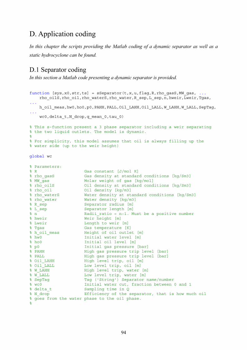
94

D. Application coding In this chapter the scripts providing the Matlab coding of a dynamic separator as well as a

static hydrocyclone can be found.

D.1 Separator coding In this section a Matlab code presenting a dynamic separator is provided. function [sys,x0,str,ts] = sSeparator(t,x,u,flag,R,rho_gasS,MW_gas, ... rho_oilS,rho_oil,rho_waterS,rho_water,R_sep,L_sep,n,hweir,Lweir,Tgas, ... h_oil_meas,hw0,ho0,p0,PAHH,PALL,Oil_LAHH,Oil_LALL,W_LAHH,W_LALL,SepTag, ... wc0,delta_t,N_drop,q_mean_0,tau_0) % This s-function present a 3 phase separator including a weir separating % the two liquid outlets. The model is dynamic. % % For simplicity, this model assumes that oil is always filling up the % water side (up to the weir height) global wc % Parameters: % R Gas constant [J/mol K] % rho_gasS Gas density at standard conditions [kg/Sm3] % MW_gas Molar weight of gas [kg/mol] % rho_oilS Oil density at standard conditions [kg/Sm3] % rho_oil Oil density [kg/m3] % rho_waterS Water density at standard conditions [kg/Sm3] % rho_water Water density [kg/m3] % R_sep Separator radius [m] % L_sep Separator length [m] % n Radii_ratio = n:1. Must be a positive number % hweir Weir height [m] % Lweir Length to weir [m] % Tgas Gas temperature [K] % h_oil_meas Height of oil outlet [m] % hw0 Initial water level [m] % ho0 Initial oil level [m] % p0 Initial gas pressure [bar] % PAHH High gas pressure trip level [bar] % PALL High gas pressure trip level [bar] % Oil_LAHH High level trip, oil [m] % Oil_LALL Low level trip, oil [m] % W_LAHH High level trip, water [m] % W_LALL Low level trip, water [m] % SepTag Tag ('String') Separator name/number % wc0 Initial water cut, fraction between 0 and 1 % delta_t Sampling time in Q % N_drop Efficiency of the separator, that is how much oil % goes from the water phase to the oil phase. %

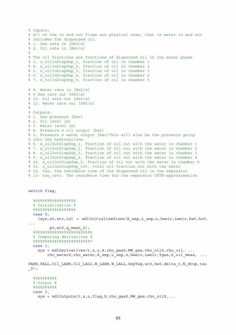
95

% Inputs: % All of the in and out flows are physical ones, that is water in and out % includes the dispersed oil. % 1. Gas rate in [Sm3/s] % 2. Oil rate in [Sm3/s] % % The oil fractions are fractions of dispersed oil in the water phase % 3. x_oilInDispSep_1, fraction of oil in chamber 1 % 4. x_oilInDispSep_2, fraction of oil in chamber 2 % 5. x_oilInDispSep_3, fraction of oil in chamber 3 % 6. x_oilInDispSep_4, fraction of oil in chamber 4 % 7. x_oilInDispSep_5, fraction of oil in chamber 5 % 8. Water rate in [Sm3/s] % 9 Gas rate out [Sm3/s] % 10. Oil rate out [Sm3/s] % 11. Water rate out [Sm3/s] % % Outputs: % 1. Gas pressure [bar] % 2. Oil level [m] % 3. Water level [m] % 4. Pressure @ oil output [bar] % 5. Pressure @ water output [bar]This will also be the pressure going % into the hydrocyclone. % 6. x_oilOutDispSep_1, Fraction of oil out with the water in chamber 1 % 7. x_oilOutDispSep_2, Fraction of oil out with the water in chamber 2 % 8. x_oilOutDispSep_3, Fraction of oil out with the water in chamber 3 % 9. x_oilOutDispSep_4, Fraction of oil out with the water in chamber 4 % 10. x_oilOutDispSep_5, Fraction of oil out with the water in chamber 5 % 11. x_oilOutDispSep_tot, total oil fraction out with the water % 12. tau, the residence time of the dispersed oil in the separator % 13- tau_cstr. The residence time for the separator CSTR-approximation switch flag, %%%%%%%%%%%%%%%%%% % Initialization % %%%%%%%%%%%%%%%%%% case 0, [sys,x0,str,ts] = mdlInitializeSizes(R_sep,L_sep,n,hweir,Lweir,hw0,ho0, ... p0,wc0,q_mean_0); %%%%%%%%%%%%%%%%%%%%%%%%% % Computing derivatives % %%%%%%%%%%%%%%%%%%%%%%%%¤ case 1, sys = mdlDerivatives(t,x,u,R,rho_gasS,MW_gas,rho_oilS,rho_oil, ... rho_waterS,rho_water,R_sep,L_sep,n,hweir,Lweir,Tgas,h_oil_meas, ... PAHH,PALL,Oil_LAHH,Oil_LALL,W_LAHH,W_LALL,SepTag,wc0,hw0,delta_t,N_drop,tau_0); %%%%%%%%%% % Output % %%%%%%%%%% case 3, sys = mdlOutputs(t,x,u,flag,R,rho_gasS,MW_gas,rho_oilS,...

96

rho_oil,rho_waterS,rho_water,R_sep,L_sep,n,hweir,Lweir,Tgas,h_oil_meas, ... hw0,ho0,p0,PAHH,PALL,Oil_LAHH,Oil_LALL,W_LAHH,W_LALL,SepTag,wc0,delta_t, ... N_drop,tau_0); %%%%%%%%%%%%% % Terminate % %%%%%%%%%%%%% case {2,4,9}, % unused flags sys = []; % do nothing %%%%%%%%%%%%%%%%%%%% % Unexpected flags % %%%%%%%%%%%%%%%%%%%% otherwise error(['unhandled flag = ',num2str(flag)]); end % %======================================================================= % mdlInitializeSizes % Return the sizes, initial conditions, and sample times for the S-function. %======================================================================= % function [sys,x0,str,ts] = mdlInitializeSizes(R_sep,L_sep,n,hweir,Lweir,hw0, ... ho0,p0,wc0,q_mean_0) global wc sizes = simsizes; sizes.NumContStates = 7; sizes.NumDiscStates = 0; sizes.NumOutputs = 13; sizes.NumInputs = 12; sizes.DirFeedthrough = 1; sizes.NumSampleTimes = 1; sys = simsizes(sizes); %calculate initial water volume if hw0 <= hweir Vw0 = WaterVol(R_sep,Lweir,L_sep,n,hweir,hw0); else errordlg('Water level above weir plate'); end wc = wc0; %caluclate initial oil volume VwWeir = cyl(hweir,R_sep,Lweir) + one_ellip(hweir,R_sep,n); Vo0 = OilVol(ho0,R_sep,Lweir,L_sep,n,hweir,Vw0); V_sep=R_sep^2*pi*L_sep+(pi/4)*(4/3)*R_sep^3; Vg0 = V_sep - Vo0 - Vw0; if ((Vg0 < 0) | (Vg0 > V_sep))

97

errordlg('Something wrong with initial gas volume'); end x0 = [hw0 ho0 Vg0 p0*1e5 Vw0 Vo0 (Vw0/q_mean_0)+10]; % initialize states str = []; ts = [0 0]; % end mdlInitializeSizes function sys = mdlDerivatives(t,x,u,R,rho_gasS,MW_gas,rho_oilS,rho_oil, ... rho_waterS,rho_water,R_sep,L_sep,n,hweir,Lweir,Tgas,h_oil_meas,PAHH, ... PALL,Oil_LAHH,Oil_LALL,W_LAHH,W_LALL,SepTag,wc0,hw0,delta_t,N_drop,tau_0) % Convert inputs persistent errorStatusOil errorStatusWater errorStatusPressure global wc if ~isfield(errorStatusOil,SepTag) errorStatusOil=setfield(errorStatusOil,SepTag,0); errorStatusWater=setfield(errorStatusWater,SepTag,0); errorStatusPressure=setfield(errorStatusPressure,SepTag,0); end % calculate water volume if water level is equal to weir height: VwWeir = cyl(hweir,R_sep,Lweir) + one_ellip(hweir,R_sep,n); % calculate oil volume if oil level is equal to weir height: VoWeir = cyl(hweir,R_sep,L_sep-Lweir) + one_ellip(hweir,R_sep,n); % -------------------------------------------------------------- % % - calculate total liquid volume if (x(1)>x(2)) % h_water > h_oil hl = x(1); else % h_oil >= h_water hl = x(2); end Vliq = cyl(hl,R_sep,L_sep) + 2*one_ellip(hl,R_sep,n); % - calculate water cut if (wc0 < 0 || wc0 > 1) errordlg(['Input water cut out of range in ' SepTag] ); end wc = wc0; if ( x(1) > hweir && x(5) < VwWeir) disp ('no') end if ( x(5) > VwWeir ) wc = (x(5) - VwWeir + wc0*x(6))/(Vliq-VwWeir); end if (wc < 0 || wc > 1) errordlg(['Calculated water cut out of range in ' SepTag] ); end

98

n_gas_in = u(1)*rho_gasS/MW_gas; % Sm3/s -> mol/s n_gas_out = u(9)*rho_gasS/MW_gas; % Sm3/s -> mol/s Q_oil_in = u(2)*rho_oilS/rho_oil; % Sm3/s -> m3/s Q_water_in = u(8)*rho_waterS/rho_water; % Sm3/s -> m3/s if t==0 Q_oilOutWoil_tot=0; end if t==0 Q_water_out=Q_water_in; else [Q_water_out,Q_oilOutWoil_tot,x_oilOutDispSep_1,x_oilOutDispSep_2, ... x_oilOutDispSep_3,x_oilOutDispSep_4,x_oilOutDispSep_5, ... x_oilOutDispSep_tot,tau]=WaterDisp(x,u,rho_oilS,rho_oil,rho_waterS, ... rho_water,R_sep,Lweir,L_sep,n,hweir,x(1),delta_t,t,N_drop,tau_0); %Q_water_out = u(11)*rho_waterS/rho_water + u(2)*rho_oilS/rho_oil*wc-Q_oilOutWoil_tot; % Sm3/s -> m3/s % Subtracting the oil separated out end Q_oil_out = u(10)*rho_oilS/rho_oil*(1-wc);%+(0.2*Q_water_in-Q_oilOutSep_tot); % options = optimset('LargeScale','off'); %options = optimset('Display','off'); q_mean= (Q_water_in+Q_water_out)/2; dqmeandt=u(12); % water volume dVwdt = (Q_water_in-Q_water_out); dVwdhw=2*Lweir*sqrt(2*R_sep*x(1)-x(1)^2)+pi/2/n^2*(2*R_sep*x(1)-x(1)^2); dTwdt=(dVwdt*q_mean-x(5)*dqmeandt)/q_mean^2; dhwdt=inv(dVwdhw)*dVwdt; if x(1) <= W_LALL & ~getfield(errorStatusWater,SepTag), errordlg(['Trip on water level (LALL) in ' SepTag] ); errorStatusWater=setfield(errorStatusWater,SepTag,1); elseif x(1) >= W_LAHH & ~getfield(errorStatusWater,SepTag), errordlg(['Trip on water level (LAHH) in ' SepTag]); errorStatusWater=setfield(errorStatusWater,SepTag,1); elseif getfield(errorStatusWater,SepTag) & (x(1) < W_LAHH) & (x(1) > W_LALL) errorStatusWater=setfield(errorStatusWater,SepTag,0); end % oil level dVodt = (Q_oil_in-Q_oil_out+Q_oilOutWoil_tot); dVldhw=2*L_sep*sqrt(2*R_sep*x(2)-x(2)^2)+pi/n^2*(2*R_sep*x(2)-x(2)^2); dhodt=inv(dVldhw)*(dVwdt+dVodt); if x(2) <= Oil_LALL & ~getfield(errorStatusOil,SepTag), errordlg(['Trip on oil level (LALL) in ' SepTag]); errorStatusOil=setfield(errorStatusOil,SepTag,1); elseif x(2) >= Oil_LAHH & ~getfield(errorStatusOil,SepTag), errordlg(['Trip on oil level (LAHH) in' SepTag]); errorStatusOil=setfield(errorStatusOil,SepTag,1);

99

elseif getfield(errorStatusOil,SepTag) & (x(2) < Oil_LAHH) & (x(2) > Oil_LALL) errorStatusOil=setfield(errorStatusOil,SepTag,0); end % Gas volume dVgdt=-(dVwdt+dVodt); V_sep=R_sep^2*pi*L_sep+(pi/4)*(4/3)*R_sep^3; % Gas pressure dngdt=n_gas_in-n_gas_out; dPdt=R*Tgas/x(3)*dngdt-x(4)/x(3)*dVgdt; if x(4) <= PALL*1e5 & ~getfield(errorStatusPressure,SepTag), errordlg(['Trip on gas pressure (PALL) in ' SepTag]); errorStatusPressure=setfield(errorStatusPressure,SepTag,1); elseif x(4) >= PAHH*1e5 & ~getfield(errorStatusPressure,SepTag), errordlg(['Trip on gas pressure (PAHH) in ' SepTag]); errorStatusPressure=setfield(errorStatusPressure,SepTag,1); elseif getfield(errorStatusPressure,SepTag) & (x(4) < PAHH*1e5) & (x(4) > PALL*1e5) errorStatusPressure=setfield(errorStatusPressure,SepTag,0); end sys=[dhwdt dhodt dVgdt dPdt dVwdt dVodt dTwdt]; % end mdlDerivatives % %======================================================================= % mdlOutputs % Return the output vector for the S-function %======================================================================= % function sys = mdlOutputs(t,x,u,flag,R,rho_gasS,MW_gas,rho_oilS,... rho_oil,rho_waterS,rho_water,R_sep,L_sep,n,hweir,Lweir,Tgas,h_oil_meas, ... hw0,ho0,p0,PAHH,PALL,Oil_LAHH,Oil_LALL,W_LAHH,W_LALL,SepTag,wc0,delta_t, ... N_drop,tau_0) %% Including a dispersed oil in water phase, with a separation efficiency %% depending on the residence time and coalescence following second order %% dynamics % Outputs: % 1. Gas pressure [bar] % 2. Oil level [m] % 3. Water level [m] % 4. Pressure @ oil output [bar] % 5. Pressure @ water output [bar] % 6. x_oilOutDispSep_1, Fraction of oil out with the water in chamber 1 % 7. x_oilOutDispSep_2, Fraction of oil out with the water in chamber 2 % 8. x_oilOutDispSep_3, Fraction of oil out with the water in chamber 3 % 9. x_oilOutDispSep_4, Fraction of oil out with the water in chamber 4 % 10. x_oilOutDispSep_5, Fraction of oil out with the water in chamber 5 % 11. x_oilOutDispSep_tot, total oil fraction out with the water % 12. tau, the residence time of the dispersed oil in the separator [Q_water_out,Q_oilOutWoil_tot,x_oilOutDispSep_1,x_oilOutDispSep_2, ... x_oilOutDispSep_3,x_oilOutDispSep_4,x_oilOutDispSep_5, ... x_oilOutDispSep_tot,tau]=WaterDisp(x,u,rho_oilS,rho_oil,rho_waterS, ... rho_water,R_sep,Lweir,L_sep,n,hweir,x(1),delta_t,t,N_drop,tau_0);

100

sys(1) = x(4)/(1e5); % Pa -> bara/bar sys(2) = x(2); % Oil level above bottom sys(3) = x(1); sys(4) = (x(4) + rho_oil*9.81*(x(2)-h_oil_meas))/(1e5); sys(5) = (x(4) + rho_oil*9.81*(x(2)-x(1)) + rho_water*9.81*x(1))/(1e5); sys(6) = x_oilOutDispSep_1; sys(7) = x_oilOutDispSep_2; sys(8) = x_oilOutDispSep_3; sys(9) = x_oilOutDispSep_4; sys(10) = x_oilOutDispSep_5; sys(11) = x_oilOutDispSep_tot; sys(12) = tau; sys(13) = x(5)/u(8);%x(7); % try % sys(6) = wc; % catch % sys(6) = wc0; % end % end mdlOutputs function [Q_water_out,Q_oilOutWoil_tot,x_oilOutDispSep_1,x_oilOutDispSep_2, ... x_oilOutDispSep_3,x_oilOutDispSep_4,x_oilOutDispSep_5, ... x_oilOutDispSep_tot,tau]=WaterDisp(x,u,rho_oilS,rho_oil,rho_waterS, ... rho_water,R_sep,Lweir,L_sep,n,hweir,hw0,delta_t,t,N_drop,tau_0) % Inputs: % All of the in and out flows are physical ones, that is water in and out % includes the dispersed oil. % 1. Gas rate in [Sm3/s] % 2. Oil rate in [Sm3/s] % % The oil fractions are fractions of dispersed oil in the water phase % 4. x_oilInSep_1, fraction of oil in chamber 1 % 5. x_oilInSep_2, fraction of oil in chamber 2 % 6. x_oilInSep_3, fraction of oil in chamber 3 % 7. x_oilInSep_4, fraction of oil in chamber 4 % The fraction of oil in chamber 5 will given by the total oil mass balance % % 8. Water rate in [Sm3/s] % 9 Gas rate out [Sm3/s] % 10. Oil rate out [Sm3/s] % 11. Water rate out [Sm3/s] % global wc %Defining the inputs x_oilInDispSep_1 = u(3); x_oilInDispSep_2 = u(4); x_oilInDispSep_3 = u(5); x_oilInDispSep_4 = u(6); x_oilInDispSep_5 = u(7); Q_water_in = u(8)*rho_waterS/rho_water; % Sm3/s -> m3/s Q_oil_in = u(2)*rho_oilS/rho_oil; % Sm3/s -> m3/s % Calculating the fraction of the remaining chamber

101

x_oilInDispSep = x_oilInDispSep_1 + x_oilInDispSep_2 + x_oilInDispSep_3 + ... x_oilInDispSep_4+x_oilInDispSep_5; Q_oilInDispSep=Q_water_in*x_oilInDispSep; x_oilInDispSep_vec = [x_oilInDispSep_1 x_oilInDispSep_2 x_oilInDispSep_3 ... x_oilInDispSep_4 x_oilInDispSep_5]; %Finding the different compartment flows QoilDispSep_in1=x_oilInDispSep_1*Q_water_in; %m3/s QoilDispSep_in2=x_oilInDispSep_2*Q_water_in; %m3/s QoilDispSep_in3=x_oilInDispSep_3*Q_water_in; %m3/s QoilDispSep_in4=x_oilInDispSep_4*Q_water_in;%m3/s QoilDispSep_in5=x_oilInDispSep_5*Q_water_in; %m3/s Q_chambers = [QoilDispSep_in1 QoilDispSep_in2 QoilDispSep_in3 ... QoilDispSep_in4 QoilDispSep_in5]; % Introducing 2nd order characteristics for the plug flow going through % Given by (1/CA)=(1/CA0)+kt. Assuming CA = x_oilInDispSep and t=tau and that % k is given by assuming complete separation after 4 minutes, and that CA at % this point equals 1 % of CA0. k1 = ((1/(0.001*x_oilInDispSep_1))-(1/x_oilInDispSep_1))/(4*60); k2 = ((1/(0.001*x_oilInDispSep_2))-(1/x_oilInDispSep_2))/(4*60); k3 = ((1/(0.001*x_oilInDispSep_3))-(1/x_oilInDispSep_3))/(4*60); k4 = ((1/(0.001*x_oilInDispSep_4))-(1/x_oilInDispSep_4))/(4*60); k5 = ((1/(0.001*x_oilInDispSep_5))-(1/x_oilInDispSep_5))/(4*60); k_vec = [k1 k2 k3 k4 k5]; persistent Qvec if t == 0 Qvec = Q_water_in; else Qvec = [Qvec Q_water_in]; end % What is denoted a/A will be going upwards/be separated out Qoil_a = 0; % What is denoted c/C on the other hand will be going % downward/exiting still dispersed in the water at the outlet. Qoil_c = 0; Q_oilOutDispSep_1 = 0; Q_oilOutDispSep_2 = 0; Q_oilOutDispSep_3 = 0; Q_oilOutDispSep_4 = 0; Q_oilOutDispSep_5 = 0; Q_oilOutWOil_1 = 0; Q_oilOutWOil_2 = 0; Q_oilOutWOil_3 = 0;

102

Q_oilOutWOil_4 = 0; Q_oilOutWOil_5 = 0; for i=1:length(Q_chambers) if t<=250 % The script should be run for some time (>= one residence time) to build % up the q-vector. (See the residence time function further down in the % script) % First the minimum efficiency based on drop size is estimated Qoil_a(i)=N_drop(i)*Q_chambers(i); Qoil_c(i)=(1-N_drop(i))*Q_chambers(i); tau=tau_0; % An initial residence time is provided for the initialisation %adding an initial residence time dependant on the script %running, put out as parameter in mask? %succeeding the separation provided from the residence time the %fluid spends in the separator comes in addition. x_oilOutDispSep(i) = x_oilInDispSep_vec(i)*(1-N_drop(i))/ ... (1+k_vec(i)*tau*x_oilInDispSep_vec(i)*(1-N_drop(i))); %Denne er i vann QoilA_tau(i)=(x_oilInDispSep_vec(i)-x_oilOutDispSep(i))*Q_chambers(i); QoilC_tau(i)=x_oilOutDispSep(i)*Q_chambers(i); % Placing the drops in their respective compartments if i==1; Q_oilOutWOil_1 = QoilA_tau(i); Q_oilOutDispSep_1 = QoilC_tau(i); elseif i==2 Q_oilOutWOil_2 = QoilA_tau(i); Q_oilOutDispSep_2 = QoilC_tau(i); elseif i==3 Q_oilOutWOil_3 = QoilA_tau(i); Q_oilOutDispSep_3 = QoilC_tau(i); elseif i==4 Q_oilOutWOil_4 = QoilA_tau(i); Q_oilOutDispSep_4 = QoilC_tau(i); elseif i==5 Q_oilOutWOil_5 = QoilA_tau(i); Q_oilOutDispSep_5 = QoilC_tau(i); end else tau = residencetime(R_sep,Lweir,L_sep,n,hweir,hw0,Qvec,delta_t); Qoil_a(i)=N_drop(i)*Q_chambers(i); % Minimum drop size efficiency. a is % separated out, c is still dispersed. Qoil_c(i)=(1-N_drop(i))*Q_chambers(i);

103

if tau<60 NA_tau=0; %0.2; NC_tau=1; %0.5; QoilA_tau(i)=0; QoilC_tau(i)=Qoil_a(i)+Qoil_c(i); elseif tau<240 x_oilOutDispSep(i) = x_oilInDispSep_vec(i)*(1-N_drop(i))/ ... (1+k_vec(i)*tau*x_oilInDispSep_vec(i)*(1-N_drop(i))); QoilA_tau(i)=(x_oilInDispSep_vec(i)-x_oilOutDispSep(i))*Q_chambers(i); QoilC_tau(i)=x_oilOutDispSep(i)*Q_chambers(i); else NA_tau=1; NC_tau=0; QoilA_tau(i)=Qoil_a(i)+Qoil_c(i); QoilC_tau(i)=0; end % Placing the drops in their respective compartments if i==1; Q_oilOutWOil_1 = QoilA_tau(i); Q_oilOutDispSep_1 = QoilC_tau(i); elseif i==2 Q_oilOutWOil_2 = QoilA_tau(i); Q_oilOutDispSep_2 = QoilC_tau(i); elseif i==3 Q_oilOutWOil_3 = QoilA_tau(i); Q_oilOutDispSep_3 = QoilC_tau(i); elseif i==4 Q_oilOutWOil_4 = QoilA_tau(i); Q_oilOutDispSep_4 = QoilC_tau(i); elseif i==5 Q_oilOutWOil_5 = QoilA_tau(i); Q_oilOutDispSep_5 = QoilC_tau(i); end end end Q_oilOutDisp_tot=Q_oilOutDispSep_1+Q_oilOutDispSep_2+Q_oilOutDispSep_3+Q_oilOutDispSep_4+Q_oilOutDispSep_5; Q_oilOutWoil_tot=Q_oilOutWOil_1+Q_oilOutWOil_2+Q_oilOutWOil_3+Q_oilOutWOil_4+Q_oilOutWOil_5; % Estimating the waterflow out Q_water_out = u(11)*rho_waterS/rho_water + u(2)*rho_oilS/rho_oil*wc + Q_oilOutWoil_tot; % Sm3/s -> m3/s %the fractions are of the total flow going out of the separator and into %the hydrocyclone

104

x_oilOutDispSep_1=Q_oilOutDispSep_1/Q_water_out; % Deviding on the total waterflow out, that is waterflow including dispersed oil x_oilOutDispSep_2=Q_oilOutDispSep_2/Q_water_out; x_oilOutDispSep_3=Q_oilOutDispSep_3/Q_water_out; x_oilOutDispSep_4=Q_oilOutDispSep_4/Q_water_out; x_oilOutDispSep_5=Q_oilOutDispSep_5/Q_water_out; x_oilOutDispSep_tot=x_oilOutDispSep_1+x_oilOutDispSep_2+x_oilOutDispSep_3+x_oilOutDispSep_4+x_oilOutDispSep_5; % This is the total oil fraction out with the water of the separator % Qoil_out_tot=Qoil_out0+Qoil_out+Q_oil_in; % Qoil_disp_out_tot=Qoil_disp_out0+Qoil_disp_out; function WaterVol = WaterVol(R,Lweir,L,n,hweir,hw) if hw <= hweir % water below weir WaterVol = cyl(hw,R,Lweir) + one_ellip(hw,R,n); else % water above weir -> This is not valid errordlg('Water above weir'); WaterVol = -1; end function OilVol = OilVol(ho,R,Lweir,L,n,hweir,Vw0) % Excluding oil on % water side if ho <= hweir % oil below weir OilVol = cyl(ho,R,L-Lweir) + one_ellip(ho,R,n); else OilVol = cyl(ho,R,L) + 2*one_ellip(ho,R,n) ... % as if only oil is in % the separator - Vw0; % Subtract water % OilVol = cyl(ho,R,L)-cyl(hweir,R,Lweir) + 2*one_ellip(ho,R,n) - % one_ellip(hweir,R,n); % Disregard water side end function cyl=cyl(h,R,L) if h<0 h=0; elseif h>2*R h=2*R; end; root = 2*R*h-h^2; cyl = L*((h-R)*sqrt(root)+R^2*(asin((h-R)/R)+pi/2)); function one_ellip=one_ellip(h,R,n) one_ellip = (pi/(2*n*n))*(R*h*h-(h*h*h)/3); function f = hoBelowWeir(ho,R,Ldiff,n,Vo) f = cyl(ho,R,Ldiff)+one_ellip(ho,R,n)-Vo; f = (f/Vo);

105

function f = hoAboveWeir(ho,R,L,n,Vo,Vw,hweir,Lweir,VoWeir) f = cyl(ho,R,L)+2*one_ellip(ho,R,n)-Vo-Vw; f = (f/(Vo+Vw)); function f = hwBelowWeir(hw,R,Lweir,n,Vw) f = cyl(hw,R,Lweir)+(pi/(2*n*n))*(R*hw*hw-(hw*hw*hw)/3)-Vw; f = (f/Vw); function f = hwAboveWeir(hw,R,L,n,Vw,VoWeir) f = cyl(hw,R,L)+2*one_ellip(hw,R,n)-VoWeir-Vw; f = (f/(Vw+VoWeir)); % function tau = residencetime(R_sep,Lweir,L_sep,n,hweir,hw0,q,delta_t) % Knowing the volume of the water phase one can find the residence time % from the equation V= delta_t ' the sum from i=j(now) to (j-tau) (which % is the time the volume element q went into the tank) over qi. % q in the function is given as a vector. That is it's necessary to have % Matlab store a number of values going in. Until enough flow has gone % through to equal the amount of the water volume, that is one residence % time, the program will not be able to run. % the % delta_t=10; tau_m=0; S=0; %the sum of the qs make up the volume the element has gone through %When this volume equals the volume of the water phase it means that the %volume has been completely exchanged. That is that the little volume %element going in is on it's way out. Giving the residence time. %Calculating the water volume of the tank % Vw=90; %Volume of the water phase Vw=WaterVol(R_sep,Lweir,L_sep,n,hweir,hw0); Vw_m=Vw/delta_t; while S <= Vw_m S=S+q(end-tau_m); % disp(S); tau_m=tau_m+1; end tau_m = tau_m - 1; tau = delta_t*tau_m; return

106

D.2 Hydrocyclone coding In this section a Matlab code presenting a static hydrocyclone is provided. function [sys,x0,str,ts] = sHydrocyclone(t,x,u,flag,rho_waterS,rho_water, ... rho_oil,rho_oilS,my,Dc,Dp,SC_underflow,n_liners) % Inputs: % u(1) - Pin, Pressure at inlet [bar] % u(2) - Qoil_oS, Overflow of oil in standard conditions [Sm3/s] % u(3) - Qoil_uS, Underflow of oil in standard conditions [Sm3/s] % u(4) - xoil_in, Fraction of the inflow that is oil % u(5) - x_oilInHyd_1, Fraction of flow to compartment 1 % u(6) - x_oilInHyd_2, Fraction of flow to compartment 2 % u(7) - x_oilInHyd_3, Fraction of flow to compartment 3 % u(8) - x_oilInHyd_4, Fraction of flow to compartment 4 % % Compartment 5, x_oilInHyd_5 will be given by the 4 other component % balances and the total mass balance Qoil_in = Qoil_u+Qoil_o % % Outputs: % sys(1) - Po, Overflow pressure [bar] % sys(2) - Pu, Underflow pressure [bar] % sys(3) - Qin, The inflow [Sm3/s] % sys(4) - N, hydrocyclone efficiency % % Fractions of oil out with the overflow % sys(5) - x_oilOutOverHyd_1, Fraction of flow overflow compartment 1 % sys(6) - x_oilOutOverHyd_2, Fraction of flow overflow compartment 2 % sys(7) - x_oilOutOverHyd_3, Fraction of flow overflow compartment 3 % sys(8) - x_oilOutOverHyd_4, Fraction of flow overflow compartment 4 % sys(9) - x_oilOutOverHyd_5, Fraction of flow overflow compartment 5 % % Fractions of oil out with the underflow % sys(10) - x_oilOutUnderHyd_1, Fraction of flow overflow compartment 1 % sys(11) - x_oilOutUnderHyd_2, Fraction of flow overflow compartment 2 % sys(12) - x_oilOutUnderHyd_3, Fraction of flow overflow compartment 3 % sys(13) - x_oilOutUnderHyd_4, Fraction of flow overflow compartment 4 % sys(14) - x_oilOutUnderHyd_5, Fraction of flow overflow compartment 5 % % Parameters: % rho_waterS Water density at standard conditions [kg/Sm3] % rho_water Water density [kg/m3] % rho_oilS Oil density at standard conditions [kg/Sm3] % rho_oil Oil density [kg/m3] % my Water viscosity % Dc Hydrocyclone diameter at the broadest [m] % Dp Particle size % SC_underflow Speed correction factor for the underflow. Correcting % the diameter of the underflow being alot smaller than % that of the cyclone [fraction 0-1] % n_liners number of liners in the cyclone % % % The following outlines the general structure of an S-function. % switch flag, %%%%%%%%%%%%%%%%%%

107

% Initialization % %%%%%%%%%%%%%%%%%% case 0, [sys,x0,str,ts]=mdlInitializeSizes; %%%%%%%%%%%%%%% % Derivatives % %%%%%%%%%%%%%%% case 1, sys=mdlDerivatives(t,x,u); %%%%%%%%%% % Update % %%%%%%%%%% case 2, sys=mdlUpdate(t,x,u); %%%%%%%%%%% % Outputs % %%%%%%%%%%% case 3, sys=mdlOutputs(t,x,u,flag,rho_waterS,rho_water,rho_oil,rho_oilS,my,Dc, ... Dp,SC_underflow,n_liners); %%%%%%%%%%%%%%%%%%%%%%% % GetTimeOfNextVarHit % %%%%%%%%%%%%%%%%%%%%%%% case 4, sys=mdlGetTimeOfNextVarHit(t,x,u); %%%%%%%%%%%%% % Terminate % %%%%%%%%%%%%% case 9, sys=mdlTerminate(t,x,u); %%%%%%%%%%%%%%%%%%%% % Unexpected flags % %%%%%%%%%%%%%%%%%%%% otherwise error(['Unhandled flag = ',num2str(flag)]); end % end sfuntmpl % %============================================================================= % mdlInitializeSizes % Return the sizes, initial conditions, and sample times for the S-function. %============================================================================= % function [sys,x0,str,ts]=mdlInitializeSizes sizes = simsizes;

108

sizes.NumContStates = 0; sizes.NumDiscStates = 0; sizes.NumOutputs = 14; sizes.NumInputs = 8; sizes.DirFeedthrough = 1; sizes.NumSampleTimes = 1; % at least one sample time is needed sys = simsizes(sizes); % initialize the initial conditions % x0 = []; % % str is always an empty matrix % str = []; % % initialize the array of sample times % ts = [0 0]; % end mdlInitializeSizes % %============================================================================= % mdlDerivatives % Return the derivatives for the continuous states. %============================================================================= % function sys = mdlDerivatives(t,x,u) sys = []; % end mdlDerivatives % %============================================================================= % mdlUpdate % Handle discrete state updates, sample time hits, and major time step % requirements. %============================================================================= % function sys = mdlUpdate(t,x,u) sys = []; % end mdlUpdate % %============================================================================= % mdlOutputs

109

% Return the block outputs. %============================================================================= function sys = mdlOutputs(t,x,u,flag,rho_waterS,rho_water,rho_oil,rho_oilS,my, ... Dc,Dp,SC_underflow,n_liners) Pin = u(1); %barg QoS = u(2); QuS = u(3); xoil_in = u(4); x_oilInHyd_1 = u(5); x_oilInHyd_2 = u(6); x_oilInHyd_3 = u(7); x_oilInHyd_4 = u(8); x_oilInHyd_5 = xoil_in-(x_oilInHyd_1+x_oilInHyd_2+x_oilInHyd_3+x_oilInHyd_4); Qo = QoS*rho_oilS/rho_oil/n_liners; Qu = QuS*rho_oilS/rho_oil/n_liners; % 1) Finding Qin from equation 1 knowing the flows going out and using a % simple mass balance Qin = Qo+Qu; % 2a) Finding Qoil_in from equation 11 knowing the inflow as well as the % oil fraction at the inlet xoil_in from equation Qoil_in=xoil_in*Qin; % 2b) Finding the Chamberflows Qoil_in1=x_oilInHyd_1*Qin; Qoil_in2=x_oilInHyd_2*Qin; Qoil_in3=x_oilInHyd_3*Qin; Qoil_in4=x_oilInHyd_4*Qin; Qoil_in5=x_oilInHyd_5*Qin; % 3) Finding deltaPo from equation 5 a=(rho_water/my)^2; a2=a*Qin; a3=a2/sqrt(rho_water); b=Dc*sqrt(rho_water); b2=b/my; b3=0.2*(b2^1.85); c=(a3/b3); deltaPo=nthroot(c,0.425); % 4) Finding Qwater_in from equation 8 Qwater_in=Qin-Qoil_in; % 5) Finding Po from equation 4 Po=Pin-(deltaPo/1e5); %bar

110

% 6) Finding Dpc from equation 3 d=abs(rho_water-rho_oil); d2=d/(my^2); e=Dc*sqrt(rho_water); e2=(e/my)^0.85; e3=0.177*e2; Dpcm=sqrt(e3/(d2*(deltaPo^0.575))); %%% Qoil_inx=[Qoil_in1 Qoil_in2 Qoil_in3 Qoil_in4 Qoil_in5]; Dpm=Dp*1e-6; %m Qoil_o1=0; Qoil_o2=0; Qoil_o3=0; Qoil_o4=0; Qoil_o5=0; k=Dpm/Dpcm; % 7) Finding the hydrocyclone efficiency from equation 9, % that is depending on the cut sizes relationship to the size of the % particles for i=1:length(Qoil_inx) N(i)=(5/6)*k(i)-(1/3); % gir N=0 for 0.4 og N=1 ved k = 1.6 if N(i)>1 N(i) = 1; elseif N(i)<0 N(i) = 0; else N(i)=N(i); end % 8) Finding Qoil_o from equation 6 % Qoil_o=N*Qoil_in; Qoil_o(i)=N(i)*Qoil_inx(i); % Keeping track of the compartments if i == 1 Qoil_o1 = Qoil_o(i); elseif i == 2 Qoil_o2 = Qoil_o(i); elseif i== 3 Qoil_o3 = Qoil_o(i); elseif i == 4 Qoil_o4 = Qoil_o(i); elseif i == 5 Qoil_o5 = Qoil_o(i);

111

end end % Introducing the limitation of flow split FS=Qo/Qin*100; if FS<1.53 N_FS=59.5*FS/100; disp('FS too small') else N_FS=91/100; end % 9) Finding Qoil_u from equation 7 % Qoil_u=Qoil_in-Qoil_o; Qoil_o1_FS = N_FS*Qoil_o1; Qoil_u1_FS = Qoil_in1-Qoil_o1_FS; Qoil_o2_FS = N_FS*Qoil_o2; Qoil_u2_FS = Qoil_in2-Qoil_o2_FS; Qoil_o3_FS = N_FS*Qoil_o3; Qoil_u3_FS = Qoil_in3-Qoil_o3_FS; Qoil_o4_FS = N_FS*Qoil_o4; Qoil_u4_FS = Qoil_in4-Qoil_o4_FS; Qoil_o5_FS = N_FS*Qoil_o5; Qoil_u5_FS = Qoil_in5-Qoil_o5_FS; Qoil_o_tot = Qoil_o1_FS + Qoil_o2_FS + Qoil_o3_FS + Qoil_o4_FS + Qoil_o5_FS; Qoil_u_tot = Qoil_u1_FS + Qoil_u2_FS + Qoil_u3_FS + Qoil_u4_FS + Qoil_u5_FS; % Checking that the over or under flow of oil does not exceed the total of these flows if Qoil_o_tot >= Qo disp('Qoil_o > Qo') Qoil_o = Qo; % Qoil_o can't be larger than Qo Qoil_u = Qoil_u_tot+(Qoil_o_tot-Qoil_o); persentage_off = (Qoil_o-Qo)/Qo; Qoil_o1_FS = Qoil_o1_FS*(1-persentage_off); Qoil_o2_FS = Qoil_o2_FS*(1-persentage_off); Qoil_o3_FS = Qoil_o3_FS*(1-persentage_off); Qoil_o4_FS = Qoil_o4_FS*(1-persentage_off); Qoil_o5_FS = Qoil_o5_FS*(1-persentage_off); Qoil_u1_FS = Qoil_inx(i)-Qoil_o1_FS; Qoil_u2_FS = Qoil_inx(i)-Qoil_o2_FS; Qoil_u3_FS = Qoil_inx(i)-Qoil_o3_FS; Qoil_u4_FS = Qoil_inx(i)-Qoil_o4_FS; Qoil_u5_FS = Qoil_inx(i)-Qoil_o5_FS;

112

elseif Qoil_u_tot >= Qu disp('Qoil_u > Qu') Qoil_u = Qu; % Qoil_u cannot be larger than Qu Qoil_o = Qoil_o_tot+(Qoil_u_tot-Qoil_u); persentage_off = (Qoil_o-Qo)/Qo; Qoil_u1_FS = Qoil_u1_FS*(1-persentage_off); Qoil_u2_FS = Qoil_u2_FS*(1-persentage_off); Qoil_u3_FS = Qoil_u3_FS*(1-persentage_off); Qoil_u4_FS = Qoil_u4_FS*(1-persentage_off); Qoil_u5_FS = Qoil_u5_FS*(1-persentage_off); Qoil_o1_FS = Qoil_inx(i)-Qoil_u1_FS; Qoil_o2_FS = Qoil_inx(i)-Qoil_u2_FS; Qoil_o3_FS = Qoil_inx(i)-Qoil_u3_FS; Qoil_o4_FS = Qoil_inx(i)-Qoil_u4_FS; Qoil_o5_FS = Qoil_inx(i)-Qoil_u5_FS; else Qoil_u = Qoil_u_tot; Qoil_o = Qoil_o_tot; % and the compartment flows remain as the originals end % 10) Finding the water flow understream, Qwater_u from equation 13 Qwater_u = Qu - Qoil_u; % 11) Finding the waterfraction of the underflow, xwater_u from equation 10 if Qu>0 xwater_u=Qwater_u/Qu; %eventually (1-xoil_u) % 12) Finding the oilfraction of the underflow, xoil_u from equation 14. xoil_u=Qoil_u/Qu; else xwater_u=0; % 12) Finding the oilfraction of the underflow, xoil_u from equation 14. xoil_u=0; end % 13)Finding the underflow density rho_u from 16 rho_u=(xoil_u*rho_oil)+(xwater_u*rho_water); % 14) Finding the oil fraction of the overflow from equation 17 xoil_o=Qoil_o/max(Qo,1e-8); % 15) Finding the water fraction at the inlet, xwater_in from 12 if Qin>0 xwater_in=Qwater_in/Qin; else xwater_in=0; end % 16) Finding the inlet density rho_in from 15 rho_in=(xoil_in*rho_oil)+(xwater_in*rho_water);

113

% The height of the inflow is then the height of half a hydrocyclone radius. % as it is placed horizontally. % The height of the underflow is zero as the reference frame has been % placed here. hin=0.5*Dc;%10*Dc-((0.26/2)*Dc); g = 9.81; %The gravity constant [m/s2] % 17) Finding Pu from equation 2 Bernoulli corrected Pu=rho_u*((((4*Qin/(pi*(Dc^2)))^2)/2)-(((4*Qu/(pi*((Dc/SC_underflow)^2)))^2)/2)+(g*hin)+(Pin*1e5/rho_in)); % the pressure in Pa for the right denomination deltaPuPa = (Pin*1e5)-Pu; deltaPu = deltaPuPa/1e5; %[bar] if Qoil_in>0 Ntot= Qoil_o/Qoil_in; else Ntot=0; end if Qo>0 x_oilOutOverHyd_1 = Qoil_o1_FS/Qo; x_oilOutOverHyd_2 = Qoil_o2_FS/Qo; x_oilOutOverHyd_3 = Qoil_o3_FS/Qo; x_oilOutOverHyd_4 = Qoil_o4_FS/Qo; x_oilOutOverHyd_5 = Qoil_o5_FS/Qo; else x_oilOutOverHyd_1 = 0; x_oilOutOverHyd_2 = 0; x_oilOutOverHyd_3 = 0; x_oilOutOverHyd_4 = 0; x_oilOutOverHyd_5 = 0; end if Qu>0 x_oilOutUnderHyd_1 = Qoil_u1_FS/Qu; x_oilOutUnderHyd_2 = Qoil_u2_FS/Qu; x_oilOutUnderHyd_3 = Qoil_u3_FS/Qu; x_oilOutUnderHyd_4 = Qoil_u4_FS/Qu; x_oilOutUnderHyd_5 = Qoil_u5_FS/Qu; else x_oilOutUnderHyd_1 = 0; x_oilOutUnderHyd_2 = 0; x_oilOutUnderHyd_3 = 0; x_oilOutUnderHyd_4 = 0; x_oilOutUnderHyd_5 = 0; end % Outputs sys(1)=Po; sys(2)=Pu/1e5; sys(3)=Qin*rho_oil*n_liners/rho_oilS; %[Sm3/s]; % Oil flows out with the overflow sys(4)=Ntot;

114

sys(5)=x_oilOutOverHyd_1; sys(6)=x_oilOutOverHyd_2; sys(7)=x_oilOutOverHyd_3; sys(8)=x_oilOutOverHyd_4; sys(9)=x_oilOutOverHyd_5; % Oil flow out with the underflow sys(10)=x_oilOutUnderHyd_1; sys(11)=x_oilOutUnderHyd_2; sys(12)=x_oilOutUnderHyd_3; sys(13)=x_oilOutUnderHyd_4; sys(14)=x_oilOutUnderHyd_5; % end mdlOutputs % % ============================================================================= % mdlGetTimeOfNextVarHit % Return the time of the next hit for this block. Note that the result is % absolute time. Note that this function is only used when you specify a % variable discrete-time sample time [-2 0] in the sample time array in % mdlInitializeSizes. % ============================================================================= % % function sys=mdlGetTimeOfNextVarHit(t,x,u) sampleTime = 1; % Example, set the next hit to be one second later. sys = t + sampleTime; % end mdlGetTimeOfNextVarHit % %============================================================================= % mdlTerminate % Perform any end of simulation tasks. %============================================================================= % function sys=mdlTerminate(t,x,u) sys = []; % end mdlTerminate