Embed Size (px)
Citation preview

Water Loss Guidelines
FEBRUARY 2010
Prepared for: Water New Zealand
By: Allan Lambert (ILMSS Ltd/Wide Bay Water Corporation), and Richard Taylor (Waitakere City Council)

Acknowledgements The authors would like to thank the review members from the Water Services Managers Group comprising Andrew Venmore (Whangarei District Council), Peter Bahrs (Tauranga City Council), Kelvin Hill (Western Bay of Plenty District Council) and Gerard Cody (Timaru District Council) who assisted in the review of these guidelines. .

WATER LOSS GUIDELINES – WATER NEW ZEALAND
Table of Contents
PREFACE............................................................................................................................................................5 COPYRIGHT ........................................................................................................................................................5 EXECUTIVE SUMMARY.........................................................................................................................................6 1.0 INTRODUCTION .......................................................................................................................................8 2.0 BACKGROUND ......................................................................................................................................13
2.1 Assessing Real Losses for Management Purposes in Large. Medium and Small Systems....13 2.2 Software: Benchloss NZ and CheckCalcsNZ...........................................................................13 2.3 Water Balance ..........................................................................................................................14 2.4 Performance Indicators.............................................................................................................16 2.5 Four Components of Real Loss Management..........................................................................19
3.0 UNDERSTANDING THE EFFECTS OF UNCERTAINTIES IN THE DATA............................................................21 3.1 Benefits of Using Confidence Limits in Water Balance and PI Calculations ............................21 3.2 Example Water Balances with all residential service connections metered at property line....21 3.3 Example Water Balance with all residential service connections unmetered ..........................25 3.4 Influence of Errors in Parameters used to calculate Performance Indicators ..........................25 3.5 Summary of Key Points in Section 3 ........................................................................................26
4.0 PRACTICAL GUIDELINES FOR REDUCING DATA ERRORS .........................................................................28 4.1 Bulk Water Metering: Own Sources, Water Imported and Water Exported .............................28 4.2 Metered Consumption and Meter Lag Adjustment...................................................................29 4.3 Customer Meter Under-Registration.........................................................................................31 4.4 Estimating Unmeasured Residential Consumption ..................................................................32 4.5 Summary of Key Points in Section 4 ........................................................................................35
5.0 REDUCING WATER LOSS: ASSESSING YOUR LOSSES AND PERFORMANCE...............................................37 5.1 Assess Current Non Revenue Water Components and Costs from a Water Balance ............37 5.2 Assess Current Real Losses from Night Flow Measurements .................................................39 5.3 Compare Real Losses Management Performance using ILI and World Bank Institute Bands 40 5.4 Assessing Snapshot ILI and World Bank Institute Bands from Night Flow Measurements ....44 5.5 Other Useful Practical Indicators: Repair Times, Burst Frequencies, Rate of Rise .................45 5.6 Summary of Key Points in Section 5 ........................................................................................46
6.0 REDUCING WATER LOSS: TUNING IN TO THE BASIC CONCEPTS...............................................................48 6.1 The importance of reliable bulk and district metering...............................................................48 6.2 Speed and quality of repairs, and Component Analysis of Real Losses..................................49 6.3 Active Leakage Control, with and without Night Flows and District Metering ..........................51 6.4 Setting Leakage Targets for Zones, and Budgeting for Economic Intervention.......................55 6.5 Network Condition and burst frequency ...................................................................................59 6.6 The many influences of Pressure Management.......................................................................61 6.7 Economic level of leakage........................................................................................................65 6.8 Key points from Section 6.........................................................................................................67
7.0 RECOMMENDED WATER LOSS STRATEGY..............................................................................................69 8.0 RESOURCES ........................................................................................................................................72 9.0 REFERENCES .......................................................................................................................................73
Water New Zealand Water Loss Guidelines February 2010

Page 4 of 102
APPENDICES ................................................................................................................................................75APPENDIX A: Using Night Flow Data To Assess Real Losses ...................................................75 APPENDIX B: Significant Modifications to BenchlossNZ and CheckCalcsNZ 2008 Upgrades80 APPENDIX C: Why %s by volume are not suitable Performance Indicators for Real Losses .82 APPENDIX D: Explaining reductions in bursts following pressure management. ...................83 APPENDIX E: Methods of Calculating Average Pressure in Distribution Systems ..................86 APPENDIX F: Meter Lag Calculations: Methods and Examples .................................................89 APPENDIX G: Additional Information on Bulk Metering..............................................................91 APPENDIX H: Typical Installation of a Water Meter and Pressure Reducing Valve .................94 APPENDIX I: Pressure Management in Waitakere City – A Case Study ....................................95
Water New Zealand Water Loss Guidelines February 2010

Preface - Copyright Page 5 of 102
Preface These Water Loss Guidelines follow on from the Benchloss New Zealand Manual and Software which was first published in April 2002, then updated in February 2008. These resources are aimed at providing water suppliers in New Zealand with the tools necessary to firstly analyse the level of water losses in a water distribution network and secondly, to move forward in reducing the level of water losses to an appropriate reasonable level for the individual supply. Copyright Water New Zealand shall retain the New Zealand Copyright and sole distribution rights in New Zealand for the Guidelines. Companies based outside New Zealand - Wide Bay Water Corporation and ILMSS Ltd - which have provided contributions to the Guidelines, including material from the existing BenchlossNZ 2008 software and User Manual, and the CheckCalcsNZ 2008 software, are authorised to use any part of the material in the Guidelines internationally, including New Zealand.
Water New Zealand Water Loss Guidelines February 2010

Executive Summary Page 6 of 102
Executive Summary Despite being one of the first countries (in 2002) to produce nationally available standard best practice water balance software based on the IWA methodology, updated in 2008, New Zealand now increasingly lags behind many other countries in using these tools. There is no national requirement in New Zealand to report and publish performance in managing non-revenue water and its components. Although a few water suppliers in the Auckland area have achieved real losses within the top World Bank Institute Band (A), in others the level of losses are still too high, and in many systems it appears that no assessments of losses have yet been made. Austria – like New Zealand, a country with a high reputation for ‘green’ environmentally friendly policies – has also recently updated its water balance and performance indicators in line with IWA best practice principles. Although in general water production costs are low, economics only plays a role in the drivers for better management – others drivers are public health, security of supply, ecology and environment. Water loss levels are also the decisive indicator for the condition of the infrastructure system, from large systems down to individual small zones. These Water New Zealand Water Loss Guidelines are aimed at providing all water suppliers in New Zealand with the means to first assess their water losses, then develop an effective water loss strategy for any distribution system, large or small. They also provide a basis for planning the ‘next steps’ in managing water losses, starting from any level. Sections 1 to 6 of the Guidelines, supplemented by Appendices A to H, and the References (many of which will be made available free of charge through a proposed addition to the Water New Zealand website) provide a wealth of technical information to those who may need to use it. At the end of each of Sections 3 to 6, there is a list of bullet points (reproduced in the Introduction) for those readers who need only to know the key aspects of each of these Sections. The recommended approach to water loss management, outlined in Section 7, is as follows: Firstly to estimate the level of losses in a network using the calculation methods available (water balance and/or minimum night flow measurements), while understanding the uncertainties around the calculations, and seeking to reduce the level of these uncertainties. Satisfactory metering of system input (bulk water supplied to a network or zone) is fundamental to these calculations. Assessment of the consumption of unmetered residential properties remains an area of uncertainty in water balances that can be reduced by using minimum night flows to assess real losses. Secondly, having established the level of water losses occurring, it is recommended that leakage targets be set for the system based on guidelines given in Section 6.4, and that budgets for installing monitoring equipment and active leakage control are prepared for approval. Guidance on how to budget for active leakage control, metering and pressure control is provided. Thirdly, the remaining actions outlined in Section 7 need to be implemented at an appropriate scale in order for set targets to be achieved within an agreed time frame, to reduce and then to maintain water losses at an acceptable level. A description of what is considered to be a basic and an advanced level of implementation of the various actions is included in Table 7.1. This requires ongoing commitment and dedication, and not only of water supply operational staff. It also requires adequate budgets for key ongoing activities; inadequate budgets do not save costs, where leakage is concerned they increase costs. In summary, there is a need for many New Zealand water suppliers to address water loss management and these guidelines are intended to be a toolbox for those wanting to make progress. Increasingly water suppliers are faced with inadequate treated water supplies, and leakage assessment and reduction must be considered as the first step in providing for future demand.
Water New Zealand Water Loss Guidelines February 2010

Executive Summary Page 7 of 102
A summary of some additional resources (manuals and software) is included in the document. On behalf of Water New Zealand and the Water Services Managers Group, I want to particularly thank Richard Taylor for his commitment and motivation in leading and managing this project, and the Waitakere City Council for supporting him in these endeavours.
Murray Gibb Chief Executive Water New Zealand
Water New Zealand Water Loss Guidelines February 2010

1.0 Introduction Page 8 of 102
1.0 Introduction In 1999/2000, recommendations for a best practice Water Balance and associated Performance Indicators were published by the Water Loss Task Force of the International Water Association (IWA) (Ref. 1). New Zealand was one of the first countries to adopt these recommendations, when in 2002 Water New Zealand (previously known as the New Zealand Water and Waste Association (NZWWA)) commissioned and published the BenchlossNZ software (Ref. 2) and associated User Manual (Ref.3). These provided a standard annual water balance for bulk metering, consumption and water loss calculations, and recommended performance indicators for Non-Revenue Water and real (physical) losses, all based on international best practice. Benchloss NZ and the Benchloss User Manual were updated in February 2008 (Refs. 4,5), to include several improvements such as the use of minimum default values for smaller components of the Water Balance, and linking of performance to the World Bank Institute banding system. Another software (CheckCalcsNZ, Ref. 6), which does the same type of calculations with some additional information on the World Bank Institute banding system (Ref. 7), and an overview of pressure management opportunities, is also available free of charge to New Zealand Water Suppliers. BenchlossNZ and CheckCalcsNZ enable Water Suppliers to establish, within calculated confidence limits, the volumes of Non-Revenue Water, Unbilled Authorised Consumption, Apparent (Commercial) Losses and Real Losses occurring in any water distribution system, and associated best practice performance indicators. These performance indicators can be used (Ref. 8) for: •• metric benchmarking (comparison of performance with other New Zealand and international
systems, allowing for key system characteristics), or •• process benchmarking (measuring progress towards targets for an individual Water
Supplier) Despite being one of the first countries to produce nationally available standard best practice Water Balance software for the IWA methodology, New Zealand now increasingly lags behind many other countries in using these tools. There is no national requirement in New Zealand to report and publish performance in managing Non-Revenue Water and its components. Although a few Utilities in the Auckland area have achieved real losses within the top World Bank Institute Band (A), in others the level of losses are still too high, and in many systems it appears that no assessments of losses have yet been made. Austria - another country with a high reputation for ‘green’ environmentally friendly policies – has also recently updated its water balance and performance indicators in line with IWA best practice principles. Although in general water production costs are low, economic aspects only play a role in the drivers for better management. Water loss levels are the decisive indicator for the condition of the infrastructure system, from large systems down to individual small zones. The OVGW W63 Austrian Standard (Ref. 9) gives the following reasons to keep water losses low: •• HYGIENIC (Public Health): each leak represents a risk of contamination by water entering
from outside the distribution system •• SUPPLY TECHNIQUES and SUPPLY SAFETY: leakage can lead to quantitative problems
(e.g, in situations of peak supply), and can cause decrease in service pressure and lead to customer complaints
•• ECOLOGICAL AND ENVIRONMENTAL ASPECTS: water losses contravene recent ecological concepts, and low water losses reduce the energy demand of pumps, treatment stations etc. and therefore reduce CO2 emissions
Water New Zealand Water Loss Guidelines February 2010

1.0 Introduction Page 9 of 102
•• ECONOMIC ASPECTS: in general high water losses cause higher running costs (e.g. energy costs, treatment chemicals, higher maintenance costs); low water losses prevent (or postpone) the exploitation of new resources
Section 7 summarises a recommended approach to a water loss strategy. Table 7.1 lists the typical activities that are considered to be appropriate for New Zealand Water Suppliers operating at a basic level and at an advanced level.
Activity 1: Categorise the Size of System as Large, Medium or Small; identify whether to use Water Balance and/or Minimum Night Flows to assess Real Losses. Activity 2a: If doing a Water Balance - even if this is an approximate first cut attempt using very basic assumptions - identify data deficiencies, use confidence limits to assess uncertainty, arrange for improvements (e.g. to bulk metering) if necessary, calculate real water losses volume and KPIs, including Infrastructure Leakage Index ILI. Activity 2b: If using Minimum Night Flows: take measurements at time of basic night consumption only, deduct estimate of customer night consumption, calculate KPIs including Snapshot ILI. Activity 3: Classify current Real Loss management performance using the World Bank Institute Banding System, and check appropriate Activity Priorities. Activity 4: Investigate Speed and Quality of Repair issues, and address deficiencies. Activity 5: Active Leakage Control: arrange for regular monitoring of minimum night flows – either by telemetry or regular use of a data logger, or (if limited budget) overnight readings in early spring and late autumn. Set intervention targets in each supply area/zone, preferably based on economic intervention; arrange for active leak detection either using in house resources or a contractor.
Activity 6: Pressure Management: ensure that you understand the various benefits of pressure management, and how pressure management might improve management of your system. Check all systems (including gravity systems) for pressure transients. Consider reducing water pressures where this is feasible. Prioritise areas based on multiple criteria (ease of introduction, measured excess pressures, high leakage/burst frequency, etc).
Activity 7: Review the condition of the network and renewal programmes, with particular emphasis on reliable recording of burst frequencies on mains and services. Valve and hydrant condition assessment and renewal programmes may also be necessary.
These activities, carried out in this order, are presented as a cost effective approach to deliver required water loss outcomes. More detailed technical information is provided, for those who will require it, in Sections 2 to 6, and Appendices A to H. Sections 3 to 6 end with bullet point summaries of Key Points, reproduced below. Section 2 includes the following: •• a classification (Table 2.1) for categorising New Zealand systems and Zones as Large,
Medium or Small, based on number of service connections; with recommendations as to whether Water Balance, or Minimum Night Flows, or both should be used to assess Real Losses, depending upon whether residential customers are metered or not.
•• where to find information on analysis of night flows (Appendix A)
Water New Zealand Water Loss Guidelines February 2010

1.0 Introduction Page 10 of 102
•• overview comments on the BenchlossNZ 2008 and CheckCalcsNZ software; more detailed information on the 2008 water balance and PI software upgrades can be found in Appendix B
•• IWA Standard Water Balance and terminology used in Benchloss and CheckCalcs (Figs 2.1 and 2.2)
•• an overview of the Performance Indicators used in Benchloss and CheckCalcs (Table 2.2) •• why %s are unsuitable for assessing operational efficiency of management of Real Losses
(see also Appendix C) •• the equation for Unavoidable Annual Real Losses (UARL) and the Infrastructure Leakage
Index (ILI) •• the World Bank Institute Banding system for categorising Real Losses (Table 2.3) •• the difference between Metric Benchmarking (for comparisons) and Process Benchmarking
(for measuring progress towards targets for an individual Water Supplier) •• recommendation to use ILI for metric benchmarking •• recommendation to use litres/conn/day or kl/km/day for process benchmarking (use
litres/service connection/day if connection density 20 per km mains or more, and kl/km/day if less than 20 service connections/km mains)
•• the ‘Four Components’ diagram for management of Real Losses (Figure 4.2) •• the additional benefits of pressure management Section 3 is provided to assist the user to understand the effects of uncertainties in the data. The key points are as follows: • ulations include data uncertainties, to a greater or lesser extent. the uncertainty can be assessed by including confidence limits in the calculations
all water balance calc•
•• •• of error in
•• ll service connections are metered, the most influential errors are
•• l Losses can be reduced, with care, to
•• ections, assessment of unmetered
•• the errors in calculation of
ection 4 provides practical guidelines for reducing data errors. The key points are as follows:
the use of confidence limits can also help to prioritise the most important sources the Water Balance for systems where a1. bulk metering accuracy (water from own sources, water imported and exported) 2. assessing billed metered consumption during the period of the water balance 3. assessing customer meter under-registration for fully metered systems, confidence limits for Reaaround +/- 30 litres/service conn./day for a system with one bulk input meter; multiple bulk input meters will tend to result in a smaller error range for systems with unmetered residential service connresidential consumption passing the property line (i.e. property boundary) dominates the sources of error, with bulk metering accuracy some way behind. confidence limits for performance indicators are dominated by Real Losses, provided reasonable care is taken in assessing number of service connections and average pressures
S•• al
•• cilities should be provided for independent checking of bulk meters
reliable bulk metering is fundamental to assessment of Non-Revenue Water and ReLosses on-site fa
•• ate for a bulk
•• ers, the less the uncertainly (Figure 4.1)
manufacturer’s in-situ testing and Flowmeter Calibration Verification Certificmeter is limited when it only relates to electronics and does not guarantee that the meter is recording the actual flow correctly the greater the number of bulk met
•• han +/- 2% Water Suppliers should aim to reduce uncertainty for bulk metering to better t•• /-
2%, depending upon the reliability of the billing systems and checking procedures administrative errors for metered consumption volumes may range between +/-0.5% and +
Water New Zealand Water Loss Guidelines February 2010
1.0 Introduction Page 11 of 102
••leted
Water Suppliers need to be aware of possible errors due to meter lag adjustments and premature water balance, before all relevant meter reading cycles have been comp
••
a logical solution to 'Premature Reporting' is to calculate their Water Balance and Real Losses Performance Indicators for a period which ends before the normal Water Year end
•• a simple graph of recorded consumption during meter reading cycles, compared with Water Supplied over the same period, can quickly identify the need for meter lag adjustments
•• default estimates of retail meter under-registration should be checked by tests on structured samples of retail meters, by type and age and/or accumulated volume
•• a consumption monitor based on a 5% random sample of unmetered residential properties may achieve an accuracy of +/- 15% (see also Fig. 4.2)
•• wider use of consumption monitors should improve the reliability of estimates of unmeasured residential consumption; geographical location and climate, household occupancy and private supply pipe leakage will be relevant factors
••
Sectilculating the Performance Indicators, using the ILI to identify performance
in the absence of consumption monitors, Water Suppliers with unmetered residential customers should use Table 4.2 for guidance when entering this data in their Water Balance.
on 5 presents information on assessing Real Losses from Water Balance or Minimum Night
Flow calculations, cabased on the World Bank Institute Banding System. Key points are as follows: •• for large and medium sized systems, the most basic method of assessing Water Losses is a
Water Balance with confidence limits, using BenchlossNZ 2008 or CheckCalcs 2008 •• data may be doubtful to start with, but the process of collecting and collating the data will
begin to highlight the gaps, and use of confidence limits helps to identify priorities for improving the water balance data.
•• in initial calculations, standard defaults should be used for Unbilled Authorised Consumption, Unauthorised Consumption and Customer Meter errors where there are large numbers of u••
r) water balance can
••
nmetered residential properties, guidance on estimates of consumption can be taken from metered residential property figures in Table 4.2, allowing for higher losses on private unmetered properties; or a 6-month (wintebe used to reduce uncertainties in the estimates. components of Non-Revenue Water are initially calculated in volume terms but can be converted to dollar equivalents using appropriate valuations for Apparent Losses, Real Losses and Unbilled Authorised Consumption
••
• PI for making comparisons of Real Losses
•• ian data set, and
•• description of performance, and a list of
•• WBI Bands
snapshot night leakage rates can be derived from night flow measurements and converted to daily snapshot leakage estimates using appropriate Night-Day Factors Infrastructure Leakage Index (ILI) is the best • management performance (Metric Benchmarking) ILIs calculated from a Water Balance can be compared to an Australasalso categorised according to the World Bank Institute Banding System (A to D) the WBI Bands provide an internationally applicablerelevant leakage management activities appropriate to each WBI Band snapshot ILIs can be calculated from night flow measurements, and classified in
••nd Rate of Rise of
Sectiand c mental to effective management of real losses:
there are several additional useful practical indicators - ‘Awareness, Location and Repair’ times, Burst Frequency Index (one for mains, another for services) aUnreported Leakage
on 6 - provides practical basic explanations of leakage and pressure management analysis oncepts that are funda
•• Section 6.1 and Appendix G provide an overview of Bulk Metering and associated problems •• reported mains bursts usually account for less than 10% of Annual Real Losses
Water New Zealand Water Loss Guidelines February 2010

1.0 Introduction Page 12 of 102
••s occur
the basic principles of Component Analysis of Real Losses, using the BABE (Bursts and Background Estimates) concept assist understanding of how and where real losse
•• real loss management deals with limiting the duration of all leaks, however small o a toilet leaking for 16 months can lose as much water as a reported mains burst
•• eaks), at a all Water Suppliers need to do Active Leakage Control (looking for unreported lfrequency appropriate to their system characteristics
•• night flow measurements in Zones are an excellent way of identifying whether there are any unreported leaks worth looking for o but take measurements at times when night consumption is at its lowest
•• a practical standard terminology for components of minimum night flows in New Zealand is roposed in Figure 6.5; please use p it to reduce misunderstandings and wasted time
th•• e IWA DMA manual (Ref 24) is an excellent source of information on setting up DMAs ••
in unavoidable real losses vary widely with average pressure and density of connections in
individual Zones; so use Snapshot ILI to set targets for night flow, and then express themlitres/connection/hour if you prefer
••
•• 00 km of mains/year) and on service connections (per
the Economic Intervention concept can be used to rapidly assess appropriate budgets for Active Leakage Control, giving the same results as more complex UK calculation methods burst frequencies on mains (per 1 1000 service connections/year) are a good indicator of network condition o and if the frequencies are high they may be reduced by pressure management
••sure management
pressure management has other benefits – reduction of leak flow rates and some components of consumption - so there is advantage to undertaking presbefore metering residential customers
••
•• all Zones should be checked for pressure transients – even Zones supplied by gravity
a rapid overview assessment of possible range of benefits of pressure management can be made with CheckCalcs
•• ssing
•• mer service and fire sprinkler systems so
•• ge 1 to 3, with
•• ILIs close to 1
w ss s stribution system, large or small. The objective of a water loss strategy
the Pressure Management Group of the IWA Water Loss Task Force is progreimproved methods of detailed predictions of pressure management benefits reducing water pressures can impact custoparticular care needs to be taken when implementing pressure management data from the UK suggests that economic ILIs are likely to be within the ranlowest values where water is most expensive and supply is actually or potentially limited experience from Australia and New Zealand (Auckland region) shows that can be achieved
These Water New Zealand Water Loss Guidelines are aimed at providing all Water Suppliers in Ne Zealand with the means to first assess their water losses, then develop an effective water
trategy for any diloshould be to reduce the level of real water losses from the water distribution network to an acceptable level based on Public Health, Customer Service, Ecological, Environmental and Economic aspects.
Water New Zealand Water Loss Guidelines February 2010

2.0 Background Page 13 of 102
2.0 Background 2.1 Assessing Real Losses for Management Purposes in Large. Medium and Small Systems Practical approaches to assessing Real Losses for the purposes of effective management differ depending upon the size of the system under consideration, and whether residential customers are metered or unmetered (it being assumed that all significant non-residential customers are metered in New Zealand). The size criteria used in Table 2.1 below to define large, medium and small are considered to be appropriate to New Zealand.
Table 2.1: Practical Approaches for Assessing Real Losses depending upon Size of System System
Number of Service
Connections
Residential customers metered?
Recommended methods for assessing Real Losses
Yes Annual water balance with confidence limits Large
> 10000 No Annual water balance with confidence limits and Zone
night flows or residential consumption monitor Yes Annual water balance with confidence limits Medium 2500 to
10000 No Zone night flow measurements to check Water Balance Yes Zone night flows or/and annual water balance
Small
< 2500 No From Zone night flow measurements Information on consumption monitors for unmeasured residential properties can be found in Appendix D of the BenchlossNZ 2008 Manual (Ref. 5). Estimates of unmeasured residential consumption passing the property boundary, made without the use of consumption monitors, can be substantially in error due not only to actual use of water by residents, but also by small numbers of long-running leaks on the private pipe between the property line (i.e. boundary line) and the buildings. For systems of ‘Small’ or ‘Medium’ size with unmeasured residential properties, it is preferable to also assess Real Losses from Zone night flow measurements rather than to set up a small and possibly unrepresentative consumption monitor. Sections 3 and 4 of these Guidelines concentrate mainly on Water Balance and Key Performance Indicator calculations with Confidence Limits. Information on basic interpretation of night flows, including the calculation of a ‘Snapshot ILI’ (Infrastructure Leakage Index) can be found in Section 5 onwards, and Appendix A of these Guidelines. 2.2 Software: Benchloss NZ and CheckCalcsNZ The objectives of the BenchlossNZ Software and its associated Manual are to: •• provide a standard terminology for components of the annual water balance calculation •• encourage Water Suppliers in New Zealand to calculate components of Non-Revenue
Water, including Apparent Losses and Real Losses, using the standard annual water balance
•• promote the use of Performance Indicators suitable for national and international benchmarking of performance in managing water losses from public water supply transmission and distribution systems.
The methodologies used in BenchlossNZ and CheckCalcsNZ draw strongly on relevant aspects of ongoing research and recommendations of the IWA Water Loss Task Force, and experiences in implementing these recommendations in New Zealand and internationally. The more significant modifications included in the 2008 upgrades to these two softwares are summarised in Appendix B.
Water New Zealand Water Loss Guidelines February 2010
2.0 Background Page 14 of 102
The two softwares are complementary to each other. Both will produce the same results for Water Balance and Performance Indicator calculations, with confidence limits, if the same data are entered. Availability of CheckCalcsNZ avoided the necessity to make the BenchlossNZ software more detailed than its existing format, and:
oo allows the user to calculate System Running Costs, in the ‘Running Costs’ Worksheet
oo compares performance of the system with an Australian/New Zealand data set, and identifies appropriate action priorities for different World Bank Institute Performance Bands A to D, in the ‘WBI Guidelines’ Worksheet
oo provides an overview of pressure management opportunities and probable range of reduction of leak flow rates, new burst frequencies and income from metered customers, in the ‘PMOpportunities’ Worksheet.
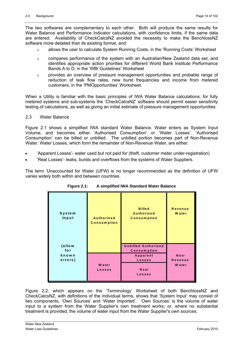
When a Utility is familiar with the basic principles of IWA Water Balance calculations, for fully metered systems and sub-systems the ‘CheckCalcsNZ’ software should permit easier sensitivity testing of calculations, as well as giving an initial estimate of pressure management opportunities. 2.3 Water Balance Figure 2.1 shows a simplified IWA standard Water Balance. Water enters as System Input Volume, and becomes either ‘Authorised Consumption’ or ‘Water Losses’. ‘Authorised Consumption’ can be billed or unbilled. The unbilled portion becomes part of Non-Revenue Water. Water Losses, which form the remainder of Non-Revenue Water, are either: •• ‘Apparent Losses’- water used but not paid for (theft, customer meter under-registration) •• ‘Real Losses’- leaks, bursts and overflows from the systems of Water Suppliers. The term ‘Unaccounted for Water (UFW) is no longer recommended as the definition of UFW varies widely both within and between countries.
Figure 2.1: A simplified IWA Standard Water Balance
B ille d R e v e n u e S y s te m A u th o r is e d W a te r
In p u t A u th o r is e d C o n s u m p tio nC o n s u m p tio n
(a llo w U n b ille d A u th o r is e dfo r C o n s u m p tio n
k n o w n A p p a r e n t N o n -e rro rs ) L o s s e s R e v e n u e
W a te r W a te rL o s s e s R e a l
L o s s e s
Figure 2.2, which appears on the ‘Terminology’ Worksheet of both BenchlossNZ and CheckCalcsNZ, with definitions of the individual terms, shows that ‘System Input’ may consist of two components, ‘Own Sources’ and ‘Water Imported’. ‘Own Sources’ is the volume of water input to a system from the Water Supplier’s own treatment works; or, where no substantial treatment is provided, the volume of water input from the Water Supplier's own sources. Water New Zealand Water Loss Guidelines February 2010

2.0 Background Page 15 of 102
Figure 2.2: Annual Water Balance used in BenchlossNZ and CheckCalcsNZ
Own Billed Revenue Sources System Authorised Water
Input Authorised ConsumptionConsumption
(allow Unbilled AuthorisedWater for Consumption
Imported bulk Apparent Non-meter Losses Revenue errors) Water Water
Losses RealLosses
Billed Unmetered Consumption
Leakage and Overflows at Service Reservoirs
up to the street/property boundary Leakage on Service Connections
Leakage on Mains
Unmetered Unauthorised Consumption
Customer Metering Under-registration
by Registered Customers
by Registered CustomersWater Supplied
Metered
Water Exported Billed Water Exported to other Systems
Billed Metered Consumption
Figure 2.2 also clearly shows that, if Water is exported to other systems, there can be a significant difference between ‘System Input’ and ‘Water Supplied’. It is also necessary to split ‘Billed Authorised Consumption’ into ‘Billed Water Exported to other Systems’ and ‘Billed Consumption by Registered Customers (Metered and Unmetered)’. Non-Revenue Water is then calculated as the difference between:
o System Input, and Billed Authorised Consumption, or o Water Supplied, and Billed Metered and Unmetered Consumption by Registered
Customers Non-Revenue Water is then split into three principal components - Unbilled Authorised Consumption, Apparent Losses and Real Losses. In the New Zealand (and Australian) Water Balances, Unbilled Authorised Consumption and Apparent Losses can be initially estimated using the following default values:
o Unbilled Authorised Consumption = 0.5% of Water Supplied
o Apparent Losses: Unauthorised Consumption = 0.1% of Water Supplied
o Apparent Losses: Customer meter under-registration = 2.0% of Billed Metered Consumption by Registered Customers
Real Losses are then derived as Non-Revenue Water minus Unbilled Authorised Consumption – Apparent Losses. The use of defaults makes it easy to complete an initial water balance. The example shown in Figure 2.3 is for an imaginary New Zealand distribution System with 250 km on mains, 10,000 service connections (all metered), and average consumption of 1000 litres/service connection/day. The water balance volumes are shown in kl/day.
Water New Zealand Water Loss Guidelines February 2010

2.0 Background Page 16 of 102
Figure 2.3. Example Water Balance, fully metered system.
Colour coding of Cells: Yellow = Data entry, Pink = Calculated values 2.4 Performance Indicators Performance Indicators are obtained by introducing relevant system parameters to facilitate comparisons between systems of different size and different characteristics. Table 2.2 from the BenchlossNZ 2008 Manual (Ref. 5) shows the five Performance Indicators (PI) considered by Water New Zealand to be most meaningful. Different PI are required for Operational and Financial purposes. The reference numbers shown (e.g. Op27) are those used in the 2nd edition (2006) of the IWA Performance Indicators Manual (Ref. 10).
Table 2.2: Water Loss Performance Indicators in BenchlossNZ and CheckCalcsNZ
Function Performance Indicator
Notes on appropriate use of this PI
Comments
Operational: Real Losses
Op27: litres/service conn./ day, when
system pressurised
Connection density 20/km mains or more
Allows for intermittent supply in international
comparisons Operational: Real Losses
Op28: m3/km of mains/ day, when
system pressurised
Connection density less than
20/km mains
Allows for intermittent supply in international
comparisons Operational: Real Losses
Op 29: Infrastructure Leakage Index ILI
(Lm x 20 + Nc)* should exceed
3000
Ratio of Current Annual Real Losses to Unavoidable
Annual Real Losses Operational: Apparent Losses
% by volume of metered
consumption (excluding Water
Exported)
Most appropriate PI for Apparent Losses in New
Zealand
Alternative PIs (% of System Input Volume, litres/conn/day) would favour Water Suppliers with less than 100% customer metering
Financial: Non-Revenue Water by cost
Fi47: Value of Non-Revenue Water as %
of annual cost of running system
Allows separate unit values in cents/Kilolitre for each component of Non-Revenue Water
* Lm = mains length (km), Nc = number of service connections Note: Nc and Ns are used interchangeably for number of service connections. Water New Zealand Water Loss Guidelines February 2010

2.0 Background Page 17 of 102
Since the early 1980’s it has been recognised that percentages are unsuitable for assessing the operational efficiency of management of real losses (leakage and overflows) in distribution systems. This is because the calculated percentages are strongly influenced by the consumption of water in each individual system, and variations in that consumption. Non-Revenue Water expressed as a % by volume of Water Supplied, although traditionally widely used, also suffers from similar significant problems to % Real Losses when used as a PI. Appendix C provides more information on this topic, in the context of the range of consumption data in New Zealand. The Financial PI Fi47 in Table 2.2 overcomes this problem by converting components of NRW into dollars, using appropriate valuations, and expressing NRW $ value as a % of annual system running costs (defined in the ‘Running Costs’ Worksheet in CheckCalcsNZ). Regarding PIs for Real Losses, the choice between Op27 (litres/service connection/day) and Op28 (kl/km mains/day) depends upon the density of service connections per km of mains. If a well managed system in a developed country has 20 or more service connections/km of mains (Nc/Lm ≥ 20), component analysis usually shows that the majority of the leakage is associated with service connections, rather than mains; so litres/service connection/day (Op27 in Table 2.2) is preferred to kl/km mains/day (Op28, which should be used in systems with Nc/Lm less than 20 service connections/km of mains). However, neither Op27 nor Op28 take account of three key system-specific factors that have a strong influence on the lowest volume of Real Losses (the ‘Unavoidable Annual Real Losses’ UARL), achievable in any particular system: •• customer meter location on service connections (relative to street/property boundary); •• the actual density of service connections (per km of mains) •• average operating pressure (leak flow rates vary, on average, linearly with pressure) By defining the ‘Point of Consumption’ for service connections in New Zealand as the street:property boundary, for both metered and unmetered properties, the first of these three variable factors is eliminated. However, it is still necessary to allow for the actual density of service connections and average operating pressure when making performance comparisons. The first IWA Water Loss Task Force developed and published, in 1999 (Ref. 11), the following equation for predicting the UARL for well maintained systems with infrastructure in good condition:
UARL (Litres/service connection/day) = (18 x Lm + 0.8 x Nc) x P where P is the average system pressure in metres (1 metre = 10 kpa) This equation has proved to be robust when applied internationally over the ten years since 1999; although some Water Suppliers in some countries have achieved these levels of Real Losses (notably Australia, during the recent drought), very few have been able to consistently achieve validated lower levels of Real Losses. The UARL is used to calculate the Infrastructure Leakage Index (ILI), a non-dimensional performance indicator for operational management of Real Losses. The ILI is the ratio of the Current Annual Real Losses (calculated from the standard Water Balance) to the system-specific Unavoidable Annual Real Losses (calculated from the above equation for UARL). Since 1999, ILIs have been calculated for many hundreds of water supply systems internationally, with values ranging from close to 1, to over 100. In 2005, the World Bank Institute, with assistance from members of the IWA Water Loss Task Force, developed an internationally applicable Banding System for categorising Real Losses (Ref. 7). The Infrastructure Leakage Index (ILI) is used to categorise operational performance in
Water New Zealand Water Loss Guidelines February 2010

2.0 Background Page 18 of 102
real loss management into one of 4 Bands, which (for Developed Countries) are as shown in Table 2.3:
Table 2.3 World Bank Institute Bands for Leakage Management in Developed Countries
Band ILI Range
Guideline Description of Real Loss Management Performance Categories for Developed Countries
A < 2.0 Further loss reduction may be uneconomic unless there are shortages; careful analysis needed to identify cost-effective leakage management
B 2.0 to < 4.0 Possibilities for further improvement; consider pressure management, better active leakage control, better maintenance
C 4.0 to < 8.0 Poor leakage management, tolerable only if plentiful cheap resources; even then, analyse level and nature of leakage, intensify reduction efforts
D
8.0 or more
Very inefficient use of resources, indicative of poor maintenance and system condition in general, leakage reduction programs imperative and high priority
In the BenchlossNZ software, the calculated ILI can be compared to the appropriate WBI Bands on the ‘Summary’ Worksheet; more details can be found in Appendix J of the 2008 Benchloss Manual (Ref. 5). In CheckCalcsNZ, the WBI Guidelines Worksheet assigns the ILI to the appropriate WBI Band, explains the WBI Banding system in more detail, and compares the system ILI with an Australian and New Zealand data set of ILIs. Around 2005, the IWA Performance Indicators Task Force began to consider the need to select the most appropriate PIs not only on the basis of Function (Financial, Operational, etc), but also to distinguish (Ref. 8) between: •• Metric benchmarking – for more demanding comparisons between Water Suppliers •• Process benchmarking –for setting targets and ongoing monitoring of progress towards
those targets. The 2008 Benchloss NZ manual recommends that: •• Infrastructure Leakage Index (Op 29) is preferable for Metric benchmarking, as it takes
account of differences in system specific key parameters (mains length, number of service connections, customer meter location, average pressure)
•• Litres/service connection/day (Op 27) or kl/km of mains/day (Op 28) (depending upon service connection density) is preferable for Process benchmarking of progress towards reaching target for reductions in Real Losses of a specific Water Supplier
Using the example Water Balance in Figure 2.3, for a system with 250 km of mains and 10,000 service connections, and assuming an average pressure of 50 metres, the Unavoidable Annual Real Losses (UARL) for this system, calculated from the IWA formula in Section 2.4 are: UARL = (18 x 250 km + 0.8 x 10000 service conns) x 50m = 625,000 lit/day = 62.5 lit/conn/day As the density of connections (40/km mains) is greater than 20/km, Table 2.3 shows that the Op27 PI of litres/service connection/day is preferred to the Op28 PI of kl/km mains/day. Real Losses are: 1227 kl/day, so PI Op27 = 1227000/10000 = 123 litres/service connection/day Real Losses PI Op29, Infrastructure Leakage Index ILI = 123/UARL = 123/62.5 = 2.0 which is at the boundary between World Bank Institute Bands A and B. Apparent Losses are:216 kl/day (12 Unbilled Authorised Consumption, 204 customer meter error), which is 2.2% of Metered Consumption. Water New Zealand Water Loss Guidelines February 2010

2.0 Background Page 19 of 102
The ILI is clearly superior for Metric benchmarking (comparisons between systems) for Real
.5 Four Components of Real Loss Management
he ‘4 Components’ diagram (Figure 2.4) is now widely used internationally to show that effective
he area of the outer rectangle represents the Current Annual Real Losses volume, which is
Figure 2.4: The four complementary leakage management activities
Losses. However, the reason it is not usually recommended for Process benchmarking (progress towards targets for reduction of Real Losses) is that pressure management will normally be an important part of any real loss reduction strategy. When excess pressures are reduced, both the CARL and the UARL volumes will reduce, so the ILI (=CARL/UARL) may not change to any significant extent. 2 Tmanagement of Real Losses for any system requires an appropriate investment in each of four basic activities. Tcontinually tending to increase as the system gets older, and new leaks and bursts occur. The four complementary leakage management activities (shown as arrows) constrain this increase, but the maximum effect they can possibly have is to reduce the Real Losses as low as the Unavoidable Annual Real Losses (UARL), indicated by the smaller box.
he Infrastructure Leakage Index (ILI) is the non-dimensional ratio of the outer area (CARL) to the
ffective management of Real Losses requires the ongoing application (forever!) of all 4 activities
Tinner area (UARL). The ILI measures how effectively the infrastructure activities in Figure 2.4 – speed and quality of repairs, active leakage control and pipe materials management – are being managed at current operating pressure. Eto each system, at levels appropriate for that system. A high ILI is a clear indication of insufficient activity in one or more of the four activities. Usually, the two activities with the quickest results and the shortest payback period are: •• ‘Speed and Quality of Repairs’ – ensure every known leak is repaired promptly and
•• kage Control’ - finding and fixing unreported leaks; appropriate budgets for
effectively ‘Active Leaeconomic intervention frequencies can now be easily calculated using 3 basic parameters (Intervention cost; variable cost of water; rate of rise of unreported leakage).
Water New Zealand Water Loss Guidelines February 2010

2.0 Background Page 20 of 102
However, if there are excess pressures and pressure transients, in a system, pressure management can be extremely effective in reducing leak flow rates and some components of consumption, and reducing the frequency of new leaks and bursts together with increasing infrastructure life. Immediate substantial reductions in burst frequency and night flows are being achieved in both developed and developing countries. Figure 2.5 shows an example from Australia where the reduction of Zone Inlet pressure of 33% in September 2003 resulted in an immediate 71% reduction in mains breaks and a 75% reduction in service breaks, which have now been maintained for seven years.
Figure 2.5: Example of reduction of mains and service bursts after pressure management
Burleigh DMA/PMA Main to Meter Corrective Maintenance
0
10
20
30
40
50
60
Mar
-99
May
-99
Jul-9
9
Sep
-99
Nov
-99
Jan-
00
Mar
-00
May
-00
Jul-0
0
Sep
-00
Nov
-00
Jan-
01
Mar
-01
May
-01
Jul-0
1
Sep
-01
Nov
-01
Jan-
02
Mar
-02
May
-02
Jul-0
2
Sep
-02
Nov
-02
Jan-
03
Mar
-03
May
-03
Jul-0
3
Sep
-03
Nov
-03
Jan-
04
Mar
-04
May
-04
Jul-0
4
Sep
-04
Nov
-04
Jan-
05
Mar
-05
Month
No.
Bre
aks
Service BreaksMains Breaks Reduction in Service Breaks 75%
Reduction in Mains Breaks 71%
Acknowledgement: Gold Coast Water
A wider international review by members of the IWA Water Loss Task Force Pressure Management Group (Ref. 12) found that, in a sample of 110 pressure management schemes from 10 countries, the % reduction in breaks averaged 1.4 times the % reduction in average pressure. However, % reductions in breaks on mains and services for pressure management in individual Zones varied more widely, from zero in some Zones to more than 3 times the % reduction in average pressure in others. Appendix D, based on Ref. 12, explains how and why this variability can occur. Benefits and payback periods of pressure management in individual Zones can now be predicted with increasing reliability using appropriate software (for example Ref. 13), leading to the situation where Zones with good potential for effective pressure management can be identified and prioritised. More information on this topic appears in Section 6.5.
Water New Zealand Water Loss Guidelines February 2010

3.0 Understanding the Effects of Uncertainties in the Data Page 21 of 102
3.0 Understanding the Effects of Uncertainties in the Data 3.1 Benefits of Using Confidence Limits in Water Balance and PI Calculations All data associated with Water Balance and Performance Indicator calculations includes errors and uncertainties. There is no such thing as a ‘perfect’ calculation. Accepting that there are uncertainties, and trying to quantify them to make rational management decisions, is a recognised part of the IWA methodology, and can in fact be used to help a Water Supplier to prioritise where to concentrate data quality control activities to improve the reliability of the Water Balance calculation, and the performance indicators that are derived from the Water Balance. The example Water Balance in Figure 2.3 will be used to demonstrate this. 3.2 Example Water Balances with all residential service connections metered at property line The example distribution system has 250 km on mains, 10,000 service connections (Residential and Non-Residential) with an average consumption of 1 kl/day, and an average pressure of 50 metres. The Unavoidable Annual Real Losses (UARL) for this system calculated from the IWA formula in Section 2.4 are 625 kl/day, 62.5 litres/conn/day. Figure 3.1 shows the simplified Water Balance from with volumes in kl/day, without confidence limits, initially assuming that all service connections are metered at the property line. The estimated components of Non-Revenue Water (Unbilled Authorised Consumption, Unauthorised Consumption and Customer meter error (under-registration) are calculated using the defaults shown, which are New Zealand and Australian national recommended defaults for well managed systems. Thee Real Losses are 123 litres/service connection/day, and the Infrastructure Leakage Index ILI is 2.0 (= 123/62.5), which is at the upper limit of World Bank Institute Band A.
Figure 3.1: Example Water Balance, fully metered system.
Colour coding of Cells: Yellow = Data entry, pink = calculated values But how reliable are the calculated figure for Non-Revenue Water and Real Losses? Should Water Suppliers be concerned about the use of defaults, even for initial calculations? And how can Water Suppliers identify priorities to improve the reliability of the Water Balance, if they
Water New Zealand Water Loss Guidelines February 2010

3.0 Understanding the Effects of Uncertainties in the Data Page 22 of 102
cannot assess the reliability of their initial calculations? These problems are solved by attaching confidence limits to each of the volumes entered into the calculation. Data errors can be systematic, or random, or a mixture of both. For example, if the check calibration of a system input meter shows that it has over-recorded by between 2% and 4%, then there is a systematic error with a best estimate of 3% over-recording of system input volume. There will also be a random error of approximately +/- 1% of the corrected system input volume. Systematic and random errors will exist in all data entered in Water Balance and Performance Indicator calculations. If systematic errors can be identified and corrected before data are entered in the Water Balance, the remaining random errors are equally likely to be greater than, or less than, the true value. A practical approach for assessing probable random errors in calculated components of NRW, Real Losses and Performance Indicators has been developed using the statistical properties of a probability distribution known as the ‘Normal’ or ‘Gaussian’ distribution. The characteristics of the Normal distribution function are explained in Appendix A of the BenchlossNZ 2008 User Manual, but can be illustrated in a simpler way for the purpose of this Guideline. After entering a ‘best estimated’ value for each input parameter, the user of either software is offered the option to enter 95% Confidence Limits, as a % value. If the user enters 95% Confidence limits for a data entry item of X%, he or she is effectively saying:
‘I think the figure I have entered is probably within +/- X % of the true value’
For example:
‘I think the figure I entered for Water Supplied is probably within +/- 3 % of the true value’
‘I think the standard defaults I used are probably within +/- 50 % of the true value’
Using the estimated 95% confidence limits entered by the user, BenchlossNZ and CheckCalcsNZ apply routine statistical calculations to calculate 95% confidence limits for derived data, such as: •• the sums or differences of volumes in the water balance (Non-Revenue Water, Real
Losses); •• performance indicators which use combinations of items with different measurement units. Figure 3.2 shows the simplified Water Balance from Figure 3.1 with volumes in kl/day, with 95% confidence limits for data entry volumes of: •• +/- 3% for 11,500 kl/day of Water Supplied •• +/- 2% for 10,000 kl/day of billed metered consumption •• +/-50% for volumes of Unbilled Authorised Consumption and Apparent Losses estimated
from the standard defaults
The resulting confidence limits for calculated volumes are: •• +/- 27% for 1500 kl/day Non-Revenue Water •• +/- 34% for 1227 kl/day Real Losses (equivalent to +/- 42 lit./service conn./day, +/- 0.7 ILI)
Water New Zealand Water Loss Guidelines February 2010

3.0 Understanding the Effects of Uncertainties in the Data Page 23 of 102
Figure 3.2: Example Water Balance, fully metered system, ILI = 2.0 with 95% confidence limits.
The random errors in the earlier items entered in the Water Balance are all accumulating in the Real Losses. But if the user wishes to narrow the confidence limits, which data entry items are the most influential, and should receive priority attention? A quick and simple way to answer this question is shown in Figure 3.3. For each ‘data entry’ Row of the Water Balance, multiply the Volume (kl/day) by the 95% CLs (%); the priorities follow the highest figures that result from doing this.
Figure 3.3: Example Water Balance, fully metered system, ILI = 2.0 with 95% CLs and Priorities.
It can now be seen clearly that the 1st priority is to improve the confidence limits for bulk meters measuring Water Supplied, with Billed Meter Consumption the 2nd Priority. Default estimates of Customer metering errors are 3rd priority, some way behind the first two, but the other defaults estimates have low priority. Suppose now that the Water Supplier makes an effort to reduce the confidence limits for Water Supplied (Bulk Metering) to +/- 2.0%. Figure 3.4 shows that the confidence limits for Non-Revenue Water fall to +/- 20%, and for Real Losses to 26%. But the priorities have not changed. Water New Zealand Water Loss Guidelines February 2010

3.0 Understanding the Effects of Uncertainties in the Data Page 24 of 102
Figure 3.4: Water Balance, fully metered system, better bulk metering, ILI = 2.0, 95% CLs & Priorities
The confidence limits used in Figure 3.4 for bulk metering and billed consumption would only be achievable by Water Suppliers with good metering and sound data checking procedures. The priorities shown are likely to be typical for most New Zealand systems where all customers are metered. Suppose now that the Water Supplier was achieving Real Losses close to the Unavoidable Annual Real Losses (UARL) of 62.5 litres/service connection/day. After adjusting the ‘Water Supplied’ in this example calculation from 11500 kl/day to 10885 kl/day to achieve this lower volume of Real Losses, Figure 3.5 shows that the Confidence limits for Real Losses have risen from 26% in Figure 3.4 at an ILI of 2, to 51%.in Figure 3.5 at a lower ILI of 1. So it’s clear that the Confidence limits expressed as a % will vary with the level of Real Losses. Figure 3.5: Water Balance, fully metered system, better bulk metering, ILI = 1.0, 95% CLs & Priorities
In practice, it is more consistent and meaningful, once the calculation has been done, to express the confidence limits for Real Losses in litres/service connection/day, rather than %s, as follows: •• In Figure 3.5, 95% CLs were +/- 51% of 62.5 litres/connection/day = +/- 32 litres/conn/day •• In Figure 3.4, 95% CLs were +/- 26% of 123 litres/connection/day = +/- 32 litres/conn/day
Water New Zealand Water Loss Guidelines February 2010

3.0 Understanding the Effects of Uncertainties in the Data Page 25 of 102
The number of bulk meters can also influence the uncertainty of the Water Supplied volume; the greater the number of bulk meters, the smaller the overall uncertainty in the total calculated system input volume. This aspect is discussed in Section 4.1. 3.3 Example Water Balance with all residential service connections unmetered Returning to the situation in Figure 3.3, with Water Supplied 11,500 kl/day and bulk meter confidence limits of +/-3%, consider the effect on confidence limits if the residential consumption (assumed to be 9000 out of the 10000 kl/day billed consumption) is not metered, but estimated (based on a random 5% sample) to have confidence limits of +/-15%. Figure 3.6 shows that the confidence limits for Real Losses have now widened to close to +/- 100% and the top priority in the Water Balance is to reduce the confidence limits for the unmetered consumption. For large systems (with more than 10,000 service connections) this could be done by setting up a structured consumption monitor, or splitting the system into Zones with measurements of night flows. However, referring to Table 2.1 of these Guidelines, it can be seen that for ‘medium and ‘small’ systems, the preferred alternative approach is to set up Zones to measure night flows, as a consumption monitor may need a large % of the properties to be metered if it is to be representative.
Figure 3.6: Water Balance, unmetered residential properties, ILI = 2.0, 95% CLs & Priorities
3.4 Influence of Errors in Parameters used to calculate Performance Indicators In any calculation of Real Losses Performance Indicators, none of the three parameters used to calculate Real Losses PIs are absolutely reliable. Mains length should usually be known quite reliably, to within +/- 1% confidence limits, with little chance of systematic error. As for Number of service connections (Nc or Ns), a frequent error in urban areas is to assume that this is equal to the number of billed properties (or accounts), Np – which can systematically over-estimate the number of service connections up to the property line. For New Zealand conditions, BenchlossNZ suggests that, for fully metered systems, the number of service connections can be assumed as being the number of metered accounts, minus the total of any sub-meters (after master meters, e.g. to shops and flats), plus the estimated number of unmetered service connections. If systematic errors are avoided, the estimate of Nc should usually be within +/- 2%. Water New Zealand Water Loss Guidelines February 2010

3.0 Understanding the Effects of Uncertainties in the Data Page 26 of 102
For systems where residential properties are not metered, the number of service connections can be counted as being the number of stop taps (tobys) at the property line, or the ratio Nc/Np can be assessed from a representative sample of data. There are several ways of estimating average pressure. Appendix E reproduces the Appendix from the Benchloss User Manual that describes them. Using these methods, it should be possible to achieve estimates of average pressure to within +/- 5% without large systematic errors. Because Performance Indicators are calculated using several different units – volumes, number of service connections, mains length (km), pressure (metres) - calculation of % confidence limits is calculated as the square root of the sum of the squared % Confidence Limits for each parameter, while the calculation of confidence limits for ILI is slightly more complex. So the confidence limits for the PI are dominated by the parameter with the greatest % error, And for Real Losses PIs, this is almost always likely to be the confidence limits for the volume of Real Losses (+/-25% or more). Table 3.7 clearly demonstrates this.
Figure 3.7: Real Losses confidence limits dominate the confidence limits for Real Losses PIs
For Density of Conns/km = 40
Parameters used for PI calculations
95% Conf. Limits +/- ILI litres/conn/d kl/km/day
Real Losses annual volume 33.0%
No. of service conns. Ns 2.0%
Mains Length Lm (km) 1.0%
Average System Pressure Pav (m) 5.0%
33.1% 33.0%
95% Conf. Limits +/- for
33.4%
Given a basic understanding of the uncertainties inherent in Water Balance and Performance Indicator calculations, as explained with examples in Sections 3.1 to 3.4 of these Guidelines, methods of reducing the confidence limits in: •• Bulk Metering •• Billed Metered Consumption and Apparent Losses (Customer Meter under-registration) •• Unmeasured Residential Consumption are discussed in Section 4 below. 3.5 Summary of Key Points in Section 3 •• All water balance calculations include data uncertainties, to a greater or lesser extent. •• The uncertainty can be assessed by including confidence limits in the calculations •• The use of confidence limits can also help to prioritise the most important sources of error in
the Water Balance •• For systems where all service connections are metered, the most influential errors are:
1. bulk metering accuracy (water from own sources, water imported and exported) 2. assessing billed metered consumption during the period of the water balance 3. assessing customer meter under-registration
Water New Zealand Water Loss Guidelines February 2010

3.0 Understanding the Effects of Uncertainties in the Data Page 27 of 102
•• For fully metered systems, confidence limits for Real Losses can be reduced, with care, to around +/- 30 litres/service conn./day for a system with one bulk input meter; multiple bulk input meters will tend to result in a smaller error range
•• For systems with unmetered residential service connections, assessment of unmetered residential consumption (passing the property line) dominates the sources of error, with bulk metering accuracy some way behind.
•• Confidence limits for performance indicators are dominated by the errors in calculation of Real Losses, provided reasonable care is taken in assessing number of service connections and average pressures
Water New Zealand Water Loss Guidelines February 2010

4.0 Practical Guidelines for Reducing Data Errors Page 28 of 102
4.0 Practical Guidelines for Reducing Data Errors 4.1 Bulk Water Metering: Own Sources, Water Imported and Water Exported If there is no bulk water meters measuring System Input, Water Imported and Water Exported then this is an absolute priority. It is not possible to make any meaningful assessment of losses without some form of bulk metering. A meter capable of measuring the expected range of inflows within +/- 2% accuracy should be installed to manufacturer’s specifications, preferably with on-site facilities for checking volumetrically or with a second meter. An insertion probe type device (around +/- 5 to 10% accuracy) is acceptable for occasional measurements but unsatisfactory as a long term installation. As telemetry (SCADA) is another potential source of data error, all bulk meters should have an on-site visual cumulative register which should be used for Water Balance or to check SCADA data. It is important to realise that a Manufacturer’s in-situ testing and Flowmeter Calibration Verification Certificate for a bulk meter is limited when it is only related to electronics and does not constitute a comprehensive check that the meter is recording the actual flow correctly. If there is only one point of supply to the system with only one meter, then the accuracy of this one meter should be checked and calibrated regularly (once per year). For larger systems with only one source and for bulk metering points for export and import of water, the installation of two meters in series should be considered as a strategy to reduce the uncertainty in the water loss calculations (see below), together with monitoring of night flows. Where one of the bulk metering components (own sources, or water imported, or water exported) is recorded using more than one bulk meter, the overall uncertainty for that particular bulk metering component is likely to be reduced, assuming that not all meters will under-record or over-record. If, for example, all bulk import meters record approximately similar volumes, the uncertainty of the total is the uncertainty of a single meter, divided by the square root of the number of meters. The greater the number of meters measuring system input, the smaller the overall uncertainty in the total calculated system input volume as shown in Figure 4.1 below. However, if the volumes passing through the input meters are not similar, the reduction in uncertainty will not be as large as shown in Figure 4.1.
Figure 4.1: Showing the relationship between meter uncertainty, number of bulk input meters, and calculated system input volume uncertainty
Uncertainty of System Input Volume decreases as number of bulk
input meters increases (assuming all register equal volumes)
0.0%
1.0%
2.0%
3.0%
4.0%
5.0%
6.0%
7.0%
0 1 2 3 4 5 6 7 8 9 10
Number of bulk input meters
Unc
erta
inty
in S
yste
m In
put
Vol
ume
Uncertainty of 1meter = +/-6%Uncertainty of 1meter = +/-4%Uncertainty of 1meter = +/-2%
Water New Zealand Water Loss Guidelines February 2010

4.0 Practical Guidelines for Reducing Data Errors Page 29 of 102
Figure 4.1 shows that, the greater the number of meters used to record the bulk metering input components of the Water Balance (water treatment plant outputs, bulk meter import points) the more reliable will be the overall assessment of ‘Own Sources’ and ‘Water Imported’ volumes. If there are several bulk input meters each with different throughputs and % uncertainty limits, the priority should be to check first those meters that have the largest value of ‘Throughput x % uncertainty’, in a similar way to the calculations in Tables 3.3 to 3.6. As a general rule, the 95% confidence limits for each component of Bulk Metering – Own Sources, Water Imported and Water Exported volume should be better than +/- 2% to try to prevent the uncertainty in the water loss calculations becoming very large. 4.2 Metered Consumption and Meter Lag Adjustment Sections 3.1 to 3.4 of these Guidelines show that, for systems where all customers are metered, assessment of metered consumption during the period of the water balance is likely to be the 2nd largest source of error, after bulk metering. Where there is universal metering, there will always be some meters where the consumption needs to be estimated due to stopping, damage, no-reads etc. Most billing systems are not designed for retrieval of data for water balance purposes, and investigation usually identifies several sources of potential ‘administrative’ errors. A range between +/-0.5% and +/-2%, depending upon the reliability of the billing systems and checking procedures, would be a reasonable default range for most Water Suppliers. Potentially the most serious error is trying to calculate the metered authorised consumption that actually occurred between the two discrete ‘dates’ at the beginning and end of the ‘Water Year’ (normally 1st July to 30th June in New Zealand). This scale of this error, known as ‘Meter Lag Adjustment’ (MLA), will depend on numerous factors as: •• the meter reading frequency (how many times per year), •• the start and finish dates of the meter reading cycle in relation to the Water Year, •• the nature of the reading cycle (rolling reading schedule or other). •• whether there are drought restrictions on consumption at the start or end of the Water Year Meter lag adjustment calculations are discussed in Appendix F. An example from an Australian system shows that, if quarterly metered consumption volumes from customer meter readings (taken in July-Sep, Oct-Dec, Jan-Mar and Apr-June) are compared with the bulk water volumes supplied during these same 4 calendar quarters, the Non-Revenue Water volume (the difference between the volumes) appears to varies widely from one meter reading cycle to the next, and in some quarters has a zero or even negative value. However, a relatively simple MLA – in the Appendix F example, attributing 50% of the recorded metered consumption in any quarter to the previous quarter, provides a reasonably consistent set of quarterly Non Revenue Water volumes. In general, New Zealand systems do not experience the multi-year droughts that may occur in large Australian water supply systems, but MLA is still an issue because of seasonal changes in consumption. Large errors in Water Balance calculations due to meter lag can normally be avoided if the problem of Meter Lag Adjustment is acknowledged and appropriately dealt with. However, there is also the problem of Premature Calculations. In New Zealand, meter reading frequencies seem to be typically 3 months for non-residential properties or large users, and 6 or 12 months for residential properties. So on 30th June, at the end of a Water Year, some of the metered consumption data that occurred during that Water Year may not be available for a further 3, 6 or 12 months. If the Water Supplier is required to provide the Water Balance calculation before all these relevant customer meters have been read, the metered consumption has to be based upon some estimated values (often those for the same
Water New Zealand Water Loss Guidelines February 2010
4.0 Practical Guidelines for Reducing Data Errors Page 30 of 102
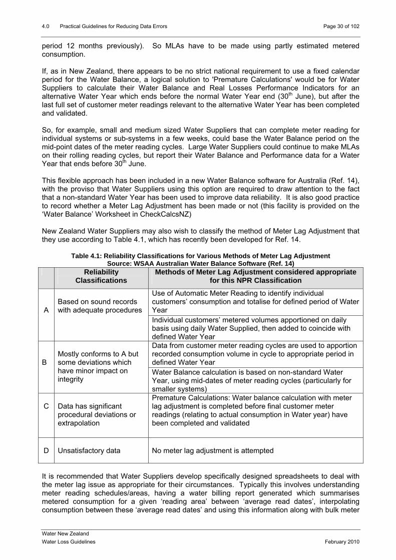
period 12 months previously). So MLAs have to be made using partly estimated metered consumption. If, as in New Zealand, there appears to be no strict national requirement to use a fixed calendar period for the Water Balance, a logical solution to 'Premature Calculations' would be for Water Suppliers to calculate their Water Balance and Real Losses Performance Indicators for an alternative Water Year which ends before the normal Water Year end (30th June), but after the last full set of customer meter readings relevant to the alternative Water Year has been completed and validated. So, for example, small and medium sized Water Suppliers that can complete meter reading for individual systems or sub-systems in a few weeks, could base the Water Balance period on the mid-point dates of the meter reading cycles. Large Water Suppliers could continue to make MLAs on their rolling reading cycles, but report their Water Balance and Performance data for a Water Year that ends before 30th June. This flexible approach has been included in a new Water Balance software for Australia (Ref. 14), with the proviso that Water Suppliers using this option are required to draw attention to the fact that a non-standard Water Year has been used to improve data reliability. It is also good practice to record whether a Meter Lag Adjustment has been made or not (this facility is provided on the ‘Water Balance’ Worksheet in CheckCalcsNZ) New Zealand Water Suppliers may also wish to classify the method of Meter Lag Adjustment that they use according to Table 4.1, which has recently been developed for Ref. 14.
Table 4.1: Reliability Classifications for Various Methods of Meter Lag Adjustment Source: WSAA Australian Water Balance Software (Ref. 14)
Reliability Classifications
Methods of Meter Lag Adjustment considered appropriate for this NPR Classification
Use of Automatic Meter Reading to identify individual customers’ consumption and totalise for defined period of Water Year
A
Based on sound records with adequate procedures
Individual customers’ metered volumes apportioned on daily basis using daily Water Supplied, then added to coincide with defined Water Year Data from customer meter reading cycles are used to apportion recorded consumption volume in cycle to appropriate period in defined Water Year
B
Mostly conforms to A but some deviations which have minor impact on integrity
Water Balance calculation is based on non-standard Water Year, using mid-dates of meter reading cycles (particularly for smaller systems)
C
Data has significant procedural deviations or extrapolation
Premature Calculations: Water balance calculation with meter lag adjustment is completed before final customer meter readings (relating to actual consumption in Water year) have been completed and validated
D
Unsatisfactory data
No meter lag adjustment is attempted
It is recommended that Water Suppliers develop specifically designed spreadsheets to deal with the meter lag issue as appropriate for their circumstances. Typically this involves understanding meter reading schedules/areas, having a water billing report generated which summarises metered consumption for a given ‘reading area’ between ‘average read dates’, interpolating consumption between these ‘average read dates’ and using this information along with bulk meter
Water New Zealand Water Loss Guidelines February 2010

4.0 Practical Guidelines for Reducing Data Errors Page 31 of 102
readings to assess water loss. Forward assessments of metered consumption in reading areas can also be made to provide for an indicative current water loss calculation. 4.3 Customer Meter Under-Registration Sections 3.1 to 3.4 of these Guidelines show that, for systems where all customers are metered, under-registration of customer meters is likely to be the 3rd largest source of error. In New Zealand and Australia, a default value of +/- 2% is recommended for apparent losses due to water meter under-registration. This figure is based on numerous studies which indicate that over time, as the accumulated volume that has passed through them increases, positive displacement water meters ‘read slowly’ and tend to under-register actual consumption. Different types of residential meters have different characteristics, and inferential (jet) meters tend to under-record low flows but over-record higher flows as they age. If there are national standards in New Zealand for replacing meters, based on age and/or accumulated volume, and most residential meters in New Zealand are 20mm positive displacement, Class C, then +/- 2% may not be an unreasonable estimate for the under-recording of positive displacement meters. However, 2% of metered consumption represents a significant volume of water. If water meters are not actually under-registering by 2%, the actual level of real water losses may be less, or more, than calculated in the water balance. Hence it is good practice to carry out a number of meter accuracy tests on a structured sample of meters to reduce the uncertainty regarding the average meter under-registration. In carrying out such tests, the overall meter accuracy should be based on a weighted average of typical consumption rates that represent the typical customer flow profiles.
Table 4.2: Recommended Domestic Meter Testing Procedure using Weighted Average Data
Test Flow Rate Assumed Usage at Given Flow Rate
Flow Test Result (inaccuracy) Weighted Result
100 litres/hour 10% X% 0.10 * X%
600 litres/hour 75% Y% 0.75 * Y%
1,500 litres/hour 15% Z% 0.15 * Z%
Sum of these three
numbers gives overall meter accuracy result
Note: It is important that correct signage of test results is used (+ve for over-registration, -ve for under-registration). Information based on a draft Australian Standard. The default assumption used in BenchlossNZ and CheckCalcsNZ is that customer meter under-registration is 2% of the true volume passing through the customer meters (not 2% of the registered volume). This is because, when customer meters are tested, the under-registration is calculated as a % of the true volume, not the recorded volume, so the correction is always a little larger than (2.04% of the recorded consumption) than users of the software expect it to be. In the example calculations in Figures 3.4 to 3.6, it has been assumed that the confidence limits for the 2% default are +/-50%, i.e. the probable range is within 1% to 3% under-registration.
Water New Zealand Water Loss Guidelines February 2010
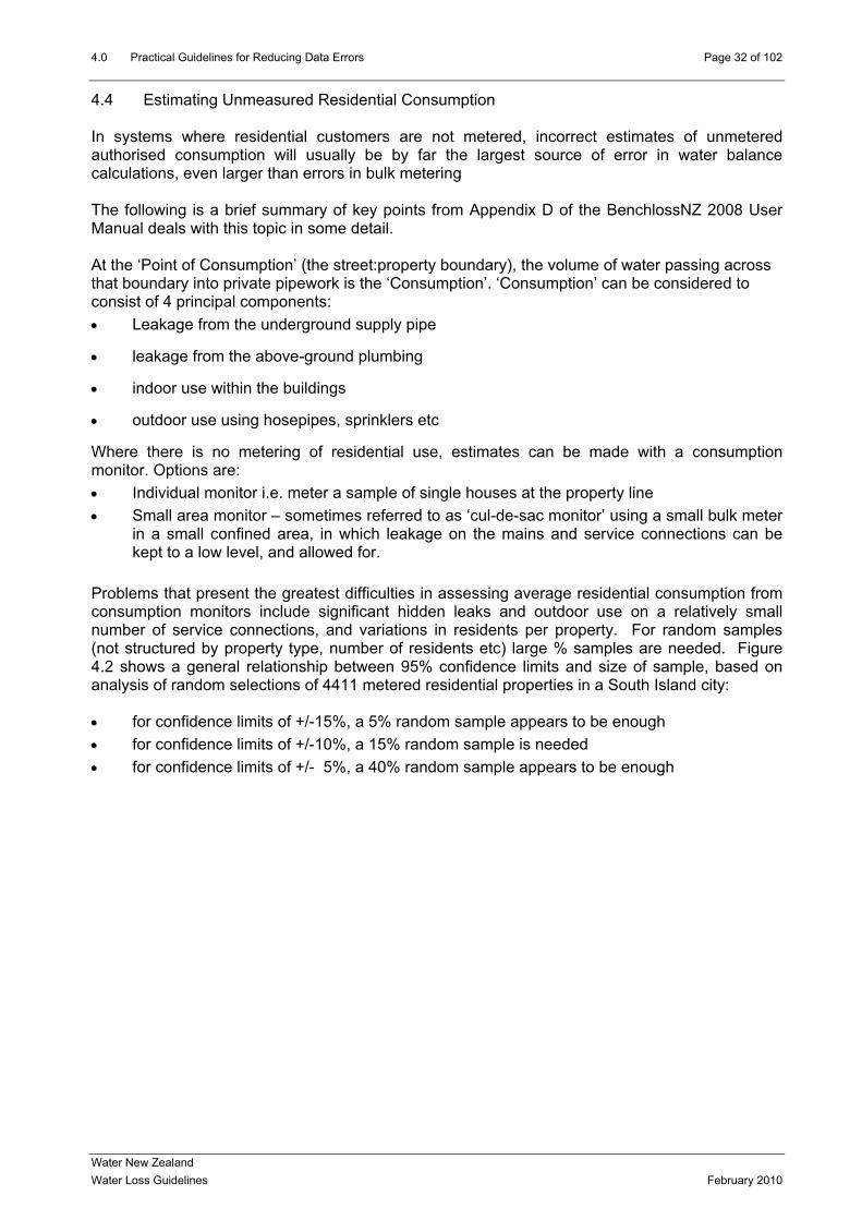
4.0 Practical Guidelines for Reducing Data Errors Page 32 of 102
4.4 Estimating Unmeasured Residential Consumption In systems where residential customers are not metered, incorrect estimates of unmetered authorised consumption will usually be by far the largest source of error in water balance calculations, even larger than errors in bulk metering The following is a brief summary of key points from Appendix D of the BenchlossNZ 2008 User Manual deals with this topic in some detail. At the ‘Point of Consumption’ (the street:property boundary), the volume of water passing across that boundary into private pipework is the ‘Consumption’. ‘Consumption’ can be considered to consist of 4 principal components: •• Leakage from the underground supply pipe
•• leakage from the above-ground plumbing
•• indoor use within the buildings
•• outdoor use using hosepipes, sprinklers etc
Where there is no metering of residential use, estimates can be made with a consumption monitor. Options are: •• Individual monitor i.e. meter a sample of single houses at the property line •• Small area monitor – sometimes referred to as ‘cul-de-sac monitor’ using a small bulk meter
in a small confined area, in which leakage on the mains and service connections can be kept to a low level, and allowed for.
Problems that present the greatest difficulties in assessing average residential consumption from consumption monitors include significant hidden leaks and outdoor use on a relatively small number of service connections, and variations in residents per property. For random samples (not structured by property type, number of residents etc) large % samples are needed. Figure 4.2 shows a general relationship between 95% confidence limits and size of sample, based on analysis of random selections of 4411 metered residential properties in a South Island city: •• for confidence limits of +/-15%, a 5% random sample appears to be enough •• for confidence limits of +/-10%, a 15% random sample is needed •• for confidence limits of +/- 5%, a 40% random sample appears to be enough
Water New Zealand Water Loss Guidelines February 2010

4.0 Practical Guidelines for Reducing Data Errors Page 33 of 102
Figure 4.2: % Sample Size vs 95% Confidence Limits, Random samples of Unmeasured Consumption in 4411 Residential Properties in a South Island City.
Because a 40% sample size appears to be needed for a consumption monitor in a small system, to be able to assess residential consumption within +/-5%, it is recommended as being preferable for medium and small systems (less than around 10,000 service connections) to assess Real Losses from Zone night flows, as this will also provide information to assist in pro-active and effective active leakage control.
-25
-20
-15
-10
-5
0
5
10
15
20
25
0 5 10 15 20 25 30 35 40 45 50 55 60 65 70 75 80 85 90 95 100
Sample size, % of total number
95%
con
fiden
ce li
mits
To assist Water Suppliers with unmetered residential customers, to use an appropriate approximate estimate of unmetered residential consumption in their Water Balance calculations, the data in Table 4.3 have been kindly provided by Water NZ members.
Table 4.3: Per Capita and per property Residential Consumption data, New Zealand
Supply/Area
Domestic Consumption
Litres/person/
day
Domestic Consumption
Litres/propert
y/day
Period of measurement
(if known)
Metered/Unmetered Y/N
If Unmetered,
number of properties surveyed
Other Comments
North Island Whangarei 179 466 2008/09 Y Rodney District:
Hibiscus Coast 165 422 2008/09 Y
based on 2.55 persons/property, single unit residential
Helensville 157 408 2008/09 Y
based on 2.60 persons/property, single unit residential
Muriwai 143 373 2008/09 Y
based on 2.60 persons/property, single unit residential
Warkworth 154 399 2008/09 Y
based on 2.60 persons/property, single unit residential
Wellsford 164 426 2008/09 Y
based on 2.60 persons/property, single unit residential
Water New Zealand Water Loss Guidelines February 2010

4.0 Practical Guidelines for Reducing Data Errors Page 34 of 102
Supply/Area
Domestic Consumption
Litres/person/
day
Domestic Consumption
Litres/propert
y/day
Period of measurement
(if known)
Metered/Unmetered Y/N
If Unmetered,
number of properties surveyed
Other Comments
Snells/Algies 116 301 2008/09 Y
based on 2.60 persons/property, single unit residential
Auckland Region: North Shore City 188 526 2008/09 Y Auckland City 160 448 2008/09 Y Waitakere City 157 471 2008/09 Y Manukau City 168 606 2008/09 Y Papakura 199 598 2008/09 Y Tauranga City 210 500 2008/09 Y Rotorua
• Eastern urban area 134 545 Jan-Oct 2009 N 14 of 3619
Average h/h occupancy 4.1for sample, 2.9 whole area
• Central urban area 219 643 Jan-Oct 2009 N 15 of 14031
Average h/h occupancy 2.9 for sample, 2.8 whole area
South Island Nelson City 175 448 2007/08 Y Tasman Region:
Collingwood 178 488 2008/09 Y
215 meters, seasonal demand
Kaiteriteri/Riwaka 172 471 2008/09 Y 574 meters Motueka 225 616 2008/09 Y 997 meters Mapua 239 654 2008/09 Y 768 meters Brightwater/Hope 260 713 2008/09 Y 973 meters Wakefield 200 547 2008/09 Y 740 meters Richmond 249 681 2008/09 Y 5108 meters Murchison 266 729 2008/09 Y 301 meters Christchurch 291 785 2005-2009 Y
Dunedin City 229 531 2008/09 N 109 of over
4000
Other monitoring suggests 580 to 600 l/property/day
Water New Zealand Water Loss Guidelines February 2010

4.0 Practical Guidelines for Reducing Data Errors Page 35 of 102
Supply/Area
Domestic Consumption
Litres/person/
day
Domestic Consumption
Litres/propert
y/day
Period of measurement
(if known)
Metered/Unmetered Y/N
If Unmetered,
number of properties surveyed
Other Comments
Clutha Region: Balclutha 508 1040 2008/09 Y Benhar 625 1200 2008/09 N 50 Restricted Supply Clinton 536 1000 2008/09 N 156 Restricted Supply Kaitangata 827 1801 2008/09 Y Lawrence 949 1285 2008/09 N 319 Milton 700 1359 2008/09 Y Owaka 520 867 2008/09 N 196 Restricted Supply Stirling 453 933 2008/09 Y Waihola 519 805 2008/09 N 174 Restricted Supply
Data from a Report (Ref. 15) by OFWAT (the Economic Regulator for England and Wales Water Utiilities) implies that, on average, real losses from unmetered private underground supply pipes are around 46 litres/property day compared to 19 litres/property/day for externally metered residential properties. In England and Wales, residential meters are also usually read every 6 months, but Water Suppliers operate intensive district metering and active leakage control, and also provide free/subsidised repairs or replacements of leaks on private supply pipes. As New Zealand Water Suppliers do not generally offer free/subsidised repairs, and most do not measure night flows, the allowance for private supply pipe losses on unmetered residential properties should be higher in New Zealand, than in England and Wales. A default figure of 66 litres/property/day was suggested in the example calculation in the CheckCalcs software (see Fig. 5.3). This is around 45 to 50 litres/residential property/day higher than the figures for externally metered residential properties in Table 4.3. 4.5 Summary of Key Points in Section 4 •• reliable bulk metering is fundamental to assessment of Non-Revenue Water and Real
Losses •• on-site facilities should be provided for independent checking of bulk meters •• manufacturer’s in-situ testing and Flowmeter Calibration Verification Certificate for a bulk
meter is limited when it only relates to electronics and does not guarantee that the meter is recording the actual flow correctly
•• the greater the number of bulk meters, the less the uncertainly (Figure 4.1) •• Water Suppliers should aim to reduce uncertainty for bulk metering to better than +/- 2% •• administrative errors for metered consumption volumes may range between +/-0.5% and +/-
2%, depending upon the reliability of the billing systems and checking procedures •• Water Suppliers need to be aware of possible errors due to meter lag adjustments and
premature water balance, before all relevant meter reading cycles have been completed •• a logical solution to 'Premature Reporting' is to calculate their Water Balance and Real
Losses Performance Indicators for a period which ends before the normal Water Year end ••
•• samples of retail meters, by type and age and/or accumulated volume
a simple graph of recorded consumption during meter reading cycles, compared with Water Supplied over the same period, can quickly identify the need for meter lag adjustments default estimates of retail meter under-registration should be checked by tests on structured
Water New Zealand Water Loss Guidelines February 2010

4.0 Practical Guidelines for Reducing Data Errors Page 36 of 102
•• a consumption monitor based on a 5% random sample of unmetered residential properties may achieve an accuracy of +/- 15% (see also Fig. 4.2)
••location and climate, household
•• is data in their Water
wider use of consumption monitors should improve the reliability of estimates of unmeasured residential consumption; geographical occupancy and private supply pipe leakage will be relevant factors in the absence of consumption monitors, Water Suppliers with unmetered residential customers should use Table 4.3 for guidance when entering thBalance.
Water New Zealand Water Loss Guidelines February 2010

5.0 Reducing Water Loss: Assessing your Losses and Performance Page 37 of 102
5.0 Reducing Water Loss: Assessing your Losses and Performance 5.1 Assess Current Non Revenue Water Components and Costs from a Water Balance For medium and large systems, Table 2.1 showed that a Water Balance with confidence limits is the most basic method of assessing Water Losses. Even though the data may be doubtful to start with, the process of collecting and collating the data will begin to highlight the gaps in the data, and the basic use of confidence limits (as shown in Tables 3.3 to 3.6) will help to identify the priorities for improving the water balance data. In BenchlossNZ 2008, the calculated Current Annual Real Losses (CARL) appear on Rows 79 to 82 of the ‘WaterBal’ Worksheet, as shown in Figure 5.1.
Figure 5.1: Current Annual Real Losses Calculation by Water Balance, BenchlossNZ 2008
The Unavoidable Annual Real Losses (UARL) are also calculated, based on the following formula of the 1st IWA Water Loss Task Force (Ref. 11), which takes into account mains length Lm (Km), number of service connections Nc and pressure (Pav, metres):
UARL (litres/day) = (18 x Lm + 0.8 x Nc) x Pav and appear on Rows 58 to 66 of the ‘ILI&UARL’ Worksheet in BenchlossNZ 2008, as shown in Figure 5.2
Figure 5.2: Calculation of UARL in BenchlossNZ 2008
In the CheckCalcs software, the calculations of Current Annual Real Losses and Unavoidable Annual Real Losses both appear on the bottom of the ‘Water Balance’ Worksheet, as shown in Figure 5.3. The $ value of the components of Non-Revenue Water (NRW) can be assessed by assigning appropriate $/m3 valuations against each of the components of NRW, as shown in the lower right hand corner of Figure 5.3. In BenchlossNZ 2008, these conversions to $NZ are done on Rows 35 to 58 of the ‘PIComps’ Worksheet.
Water New Zealand Water Loss Guidelines February 2010

5.0 Reducing Water Loss: Assessing your Losses and Performance Page 38 of 102
Figure 5.3: Calculation of CARL, UARL and NRW $NZ values in CheckCalcs
Colour coding of Cells: Yellow = Data entry, pink = calculated values, purple = defaults For your initial water balance calculations, it is recommended to use the standard defaults for Unbilled Authorised Consumption, Unauthorised Consumption, and Customer Meter under-registration (as shown above). If your system has large numbers of unmetered residential properties: •• it is recommended to use the ‘per residential property’ data figures of other New Zealand
Water Suppliers in Table 4.3 for guidance, remembering to allow for the higher real losses on unmetered supply pipes
•• an alternative possibility is to do the Water Balance over the 6 monthly winter period (April to September) when the component of garden watering should be significantly lower and the estimate of unmetered residential consumption lower, but more reliable
The Unit value of Apparent Losses is usually taken as the retail sales price for residential consumption. The Unit Value of Real Losses depends upon local circumstances; e.g. for Water Imported use the variable Bulk Supply charge plus any additional local treatment and power costs. For 'own sources', use the marginal cost/kl of treatment (chemicals) and power, plus (if appropriate) other elements such as capital deferment. Unbilled Authorised Consumption is often valued at the Unit Value of Real Losses In the example above, the initial best estimate is that this system has: •• Current Annual Real Losses of 1088 Ml/year (3.0 Ml/d) +/- 15%, valued at $109k per year •• Unavoidable Annual Real Losses of 484 Ml/year (1.3 Ml/d) +/- 5%, valued at $48k per year
Water New Zealand Water Loss Guidelines February 2010

5.0 Reducing Water Loss: Assessing your Losses and Performance Page 39 of 102
Using this approach, any New Zealand Water Utility can begin to make an assessment of their volumes of Non-Revenue Water and Real Losses, in both volume and dollar terms, with confidence limits. An alternative approach to assessing Real Losses from night flow measurements in for small systems, and Zones within larger systems, is described in Section 5.2 below. 5.2 Assess Current Real Losses from Night Flow Measurements Table 2.1 shows that Zone night flow measurements are recommended for assessing Real Losses not only in Zones of medium and large systems, but also in small systems (those with fewer than around 2500 service connections), and particularly for Zones and Systems with large numbers of unmetered residential properties. Briefly, the approach, which is explained in Appendix A, is as follows: •• arrange to measure night flows into Zone (permanent/temporary meter, reservoir drop test) •• arrange to measure or estimate an average pressure (AZNP) at night in the Zone at the
‘Average Zone Point (AZP)’, see Appendix E •• choose a time of year and days of the week when night consumption is likely to be at a
minimum, with no use of hosepipes, sprinklers or other exceptional night use •• measure the Minimum Night Flow MNF over 1 hour between 0100 and 0300 hours, together
with the Average Zone Night Pressure (preferably over several nights, and use the average values)
•• deduct estimate of Customer Night Consumption in litres/connection/hour (assumed as 2.0 litres/conn/hour +/- 40% in the example below)
•• calculate Snapshot Night Leakage Rate in m3/hour, preferably with confidence limits, as shown in Table 5.4
Figure 5.4: Example calculation of Snapshot Night Leakage Rate
Colour coding of Cells: Yellow = Data entry, pink = calculated values Using the Snapshot Night Leakage Rate of 16.8 m3/hour, the Snapshot ILI can be calculated as shown in Section 5.4 and Fig 5.12 To convert a night leakage rate in m3/hour, to an average daily leakage rate in m3/day, it is necessary to multiply by a Night-Day Factor NDF (see Appendix A), with units of Hours/day, as shown in the example in Table 5.5. The term ‘Hour-Day Factor’ is also used in the UK.
Water New Zealand Water Loss Guidelines February 2010

5.0 Reducing Water Loss: Assessing your Losses and Performance Page 40 of 102
Figure 5.5: Example Conversion of Snapshot Night Leakage Rate to Snapshot Daily Leakage,
using Night-Day Factor
Colour coding of Cells: Yellow = Data entry, pink = calculated values For Zones supplied by gravity, Night-Day Factors typically vary from 18 to 23 hours/day. Zones with pumped or pressure-modulated inflow typically have NDFs ranging from 24 to over 30 hours/day, as pressures at night (and leak flow rates) are then lower at night than during the day. Zone-specific Night-Day Factors can be calculated by taking pressure measurements at the ‘Average Zone Point’, using an appropriate FAVAD N1 value (between 0.5 and 1.5) for the pressure: leak flow rate relationship (see Section 6.6). The ‘PressCalcs’ Standard software (Ref. 13) includes a more comprehensive explanation and Worksheets to define the AZP point, estimate N1 values, and calculate NDFs from pressure measurements at the Average Zone Point. Using this approach, any New Zealand Water Utility can begin to make an assessment of the Real Losses within individual small systems and Zones, in volume terms, with confidence limits. 5.3 Compare Real Losses Management Performance using ILI and World Bank Institute
Bands Performance indicators are discussed in Section 2.4 of these Guidelines, where it has been explained that the Infrastructure Leakage Index (ILI) is the best PI for Metric benchmarking (comparisons between systems) of Real Losses management performance. The ILI is the ratio of the Current Annual Real Losses (CARL) divided by the Unavoidable Annual Real Losses (UARL, calculated from the IWA formula in Section 5.1). Figure 5.6 is a useful diagram, which explains the ILI visually and also shows how Real Losses and ILI are influenced by the four major methods of managing Real Losses. The area of the outer rectangle represents the Current Annual Real Losses volume, which is continually tending to increase as the system gets older, and new leaks and bursts occur. The four complementary leakage management activities (shown as arrows) constrain this increase, but the maximum effect they can possibly have is to reduce the Real Losses as low as the Unavoidable Annual Real Losses (UARL), indicated by the smaller box. The Infrastructure Leakage Index is the ratio of the outer area (CARL) to the inner area (UARL), and is a non-dimensional number. An ILI close to 1 represents excellent performance in managing Real Losses; whereas an ILI of, say, 5, means that the Current Real Losses are 5 times what would be expected for a well managed system with good infrastructure, at the specified average pressure.
Water New Zealand Water Loss Guidelines February 2010

5.0 Reducing Water Loss: Assessing your Losses and Performance Page 41 of 102
Figure 5.6: The 4 Components Approach to Managing Real Losses
The ILI is preferred for making comparisons between system performance, as the UARL (which is used to calculate the ‘best achievable’ Real Losses) takes into account the key system-specific factors of number of service connections, mains length and average pressure. Referring to Figure 5.6, ILI measures how well a Water Supplier is managing the East, South and West arrows (Speed and Quality of Repairs, Pipe Materials management, Active Leakage Control) at the current Operating Pressure. But this should not be taken to imply that the current operating pressure is the optimal operating pressure. Pressure management will normally be an important part of any real loss reduction strategy. And, when excess pressures are reduced, both the CARL and the UARL volumes will reduce, so the ILI (=CARL/UARL) may not change to any significant extent. Because of this effect, ILI is not normally recommended for Process benchmarking (progress towards targets for reduction of Real Losses). Litres/service connection/day, or kl/km of mains/day are preferred, depending upon whether the system connection density is more than, or less than, 20 service connections/km of mains. In BenchlossNZ 2008, the calculated ILI (with confidence limits) can be found on Row 36 of the ‘Summary’ Worksheet, as shown in Figure 5.7. In the example shown, the ILI has been assessed as being 2.25, which implies (see Columns 4 to 7 of Figure 5.7) that it is within the lower half of World Bank Institute Band B (ILI 2 to <4). The 95% confidence limits are 1.89 (lowest) to 2.60 (highest). The WBI Banding system is explained in Section 2.4. and Table 2.3, and Figures 5.10 and 5.11.
Water New Zealand Water Loss Guidelines February 2010

5.0 Reducing Water Loss: Assessing your Losses and Performance Page 42 of 102
Figure 5.7: Performance Indicators calculated using BenchlossNZ 2008
In CheckCalcs NZ, the ILI appears in Row 12 of the ‘Performance Indicators’ Worksheet, as shown in Figure 5.8, and the value is carried forward automatically to the ‘WBI Guidelines’ Worksheet, from which Figures 5.9, 5.10 and 5.11 are copied.
Figure 5.8: Excerpt from ‘Performance Indicators’ Worksheet, CheckCalcsNZ 2008
Figure 5.9 then compares the calculated ILI to the ILIs for 23 Australasian Water Suppliers.
Water New Zealand Water Loss Guidelines February 2010
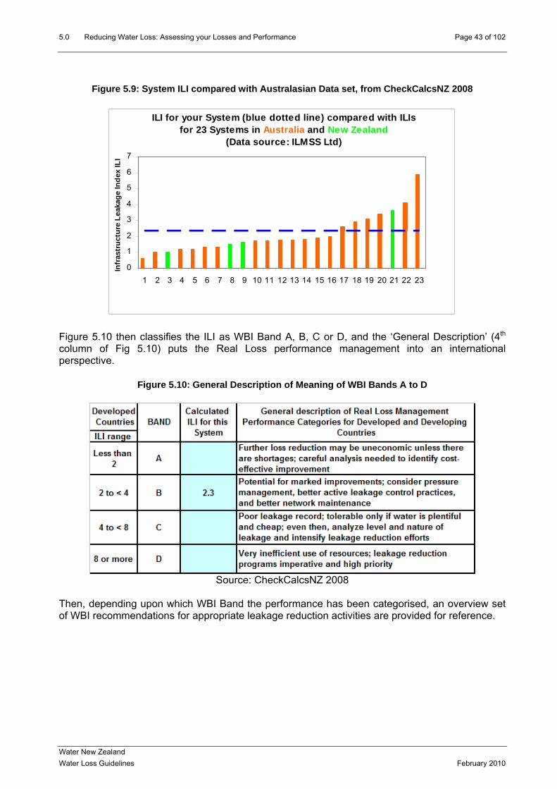
5.0 Reducing Water Loss: Assessing your Losses and Performance Page 43 of 102
Figure 5.9: System ILI compared with Australasian Data set, from CheckCalcsNZ 2008
ILI for your System (blue dotted line) compared with ILIs for 23 Systems in Australia and New Zealand
(Data source: ILMSS Ltd)
0
1
2
3
4
5
6
7
1 2 3 4 5 6 7 8 9 10 11 12 13 14 15 16 17 18 19 20 21 22 23
Infr
astr
uctu
re L
eaka
ge In
dex
ILI
Figure 5.10 then classifies the ILI as WBI Band A, B, C or D, and the ‘General Description’ (4th column of Fig 5.10) puts the Real Loss performance management into an international perspective.
Figure 5.10: General Description of Meaning of WBI Bands A to D
Source: CheckCalcsNZ 2008
Then, depending upon which WBI Band the performance has been categorised, an overview set of WBI recommendations for appropriate leakage reduction activities are provided for reference.
Water New Zealand Water Loss Guidelines February 2010

5.0 Reducing Water Loss: Assessing your Losses and Performance Page 44 of 102
Figure 5.11: Recommendations associated with WBI Bands A to D
YesFundamental peer review of all activities
YesCheck economic intervention frequency YesInvestigate speed and quality of repairs
Yes
Yes
YesYes
Yes
Deal with deficiencies in manpower, training and communications
Review asset management policy
Introduce/improve active leakage control Yes
Yes Yes
Assess Economic Leakage Level Yes
Yes
Yes
WBI Recommendations for BANDS A
Yes
Yes
Yes
Yes Yes
Yes Yes
Yes5-year plan to achieve next lowest band
DB C
Review break frequencies
YesInvestigate pressure management options
Identify options for improved maintenance Yes Yes
Source: CheckCalcsNZ 2008
So, the ILI calculated from either the BenchlossNZ or CheckCalcs Water Balance can be quickly: •• compared to a national Australasian set of ILIs (Figure 5.9) •• categorised in World Bank Institute A/B/C/D Bands, with performance description (Fig. 5.10) •• assessed for appropriate Real Losses management activities (Figure 5.11). 5.4 Assessing Snapshot ILI and World Bank Institute Bands from Night Flow Measurements Section 5.2 (and Figures 5.4 and 5.5) showed how Snapshot Night Leakage Rate can be assessed from night flow measurements in a small system or Zone. The Snapshot Night Leakage Rate can also be quickly converted into a Snapshot ILI, then categorised within the World Bank Institute Bands A to D, as shown in Figure 5.12
Figure 5.12: Calculation of Snapshot ILI and WBI Band from Snapshot Night Leakage Rate
STEP 3: CALCULATE SNAPSHOT VALUES OF REAL LOSSES PERFORMANCE INDICATORS
335.6 m3/day The Snapshot Daily Leakage is
101 litres/connection/day +/- 16.8%
The Snapshot Night Leakage Rate is 16.78 m3/hour at 59 metres AZNP
The Unavoidable Annual Real Losses are 8.59 m3/hour at 59 metres pressure
So 'Snapshot' Infrastructure Leakage Index is 1.95 which is in WBI Band A
In this example, Unavoidable Annual Real Losses UARL is calculated from the formula:
UARL (m3/hour) = (18 x Lm + 0.8 x Nc) x AZNP/24/1000 Lm = mains length (km), Nc = No. of service connections, AZNP = Ave. Zone Night pressure (m) So UARL at AZNP = (18 x 47 + 0.8 x 3310) x 59/24000 =(846+2648)x0.00246 = 8.6 m3/hr
Water New Zealand Water Loss Guidelines February 2010

5.0 Reducing Water Loss: Assessing your Losses and Performance Page 45 of 102
Calculate Snapshot ILI = Snapshot Night Leakage Rate/UARL = 16.78 / 8.6 = 2.0 The Snapshot ILI under the WBI Banding System; in this example just within Band A. ‘Snapshot’ ILIs are a very useful and practical approach for getting a quick estimate of the approximate scale of leakage in small Zones, for providing a cross-check on estimates of ILI from annual Water Balances, and for classifying Real Losses management performance using the WBI Bands A to D. However, ‘Snapshot’ ILIs derived from different limited sets of night flows will vary around the annual ILI value, and may even be less than 1.0 soon after an active leakage control intervention, when all detectable reported and unreported bursts have been repaired, and only background leaks (non-visible, non-audible) remain. So a ‘Snapshot’ ILI should always be considered as being an approximate value, always treated with caution, and always referred to as a ‘Snapshot’ value to avoid confusion with the ILI calculated from an annual water balance. 5.5 Other Useful Practical Indicators: Repair Times, Burst Frequencies, Rate of Rise High and increasing water losses are an indicator of ineffective planning and construction, and low operational maintenance activities (Ref. 16). However, there are some additional indicators now being used or tested by the IWA Water Loss Task Force, that are proving to be useful and practical in analysis of system data, to gain insights into the probable most cost-effective improvements in performance. Speed and Quality of Repairs: the ‘West’ arrow of the 4 Components Diagram (Figure 5.6) relates to Speed and Quality of Repairs. The total run time of leaks consists of 3 components: •• Awareness – from when a leak starts, until the Water Supplier becomes aware of it •• Location – the time taken to locate the leak •• Repair – the time taken to repair or shut off the leak In the absence of night flow measurements, it can be difficult to estimate Awareness times. But all Water Suppliers should keep reliable records on their Location and Repair times, for every type of leak. Long running leaks with low flow rates are the largest source of annual Real Losses. Burst Frequencies: A recent international analysis (Ref. 12) has clearly demonstrated that the burst frequencies on mains and service connections can be significantly reduced in many systems by pressure management – by reduction of pressure transients and excess pressures. Although mains bursts contribute less to annual real losses than many people imagine (usually less than 10% by volume, see Section 6.2), reduction of annual repair costs and extension of infrastructure life are now recognised as key financial drivers for pressure management. Accordingly, Water Suppliers should record their mains repairs and service connection repairs in formats that permit the calculation of monthly numbers and annual frequencies as follows: •• Mains repairs expressed in number/100 km/year •• Service connection repairs in number per 1000 service connections per year. Service connection repairs should be subdivided into: •• repairs at the ferrule/main joining point ••
•• repairs on the stop tap/toby or external meter. repairs on the service line between the main and the stoptap/toby or external meter
Water New Zealand Water Loss Guidelines February 2010

5.0 Reducing Water Loss: Assessing your Losses and Performance Page 46 of 102
These repair frequencies can then be compared to the reference frequencies for well managed infrastructure in the UARL formula of: 13 per 100 km /year for mains repairs ••
•• r services (excluding stop taps/tobys, meter repairs)
eparate values of a Burst Frequency Index (BFI) can then be calculated for mains, and for
3 per 1000 service connections/year fo Sservices. For example, if the mains burst frequency is 15 per 100 km/year and the service pipe burst frequency is 21 per 1000 service connections/year: The Burst Frequency Index for mains is 15/13 = 1.15•• , which is close to 1 ••
ese m,
The Burst Frequency Index for services is 21/3 = 7, which is high.
h two BFIs provide a quick indication of the propensity for bursts in the distribution systeTand are valuable (Ref 12) when predicting if pressure management will reduce: both mains bursts and service pipe bursts ••
•• mains bursts, but not service pipe bursts •• service pipe bursts, but not mains bursts •• ts
eter that has not traditionally been calculated,
te of Rise, and calculating Economic Intervention arameters for Active Leakage Control (the ‘East’ Arrow of 4 Components Diagram (Figure 5.6).
neither mains bursts nor service pipe burs Rate of Rise of Unreported Leakage is a parambut it is one of three parameters (the others are Variable Cost of Water, and Intervention Cost) that can be used (Ref. 17) to quickly calculate the economic frequency of intervention for active leakage control, and the associated budgets. There are 3 basic methods of assessing RapSee Section 6.4, ‘Budgeting for Economic Intervention’ for more information on this topic. 5.6 Summary of Key Points in Section 5 •• fo e most basic method of assessing Water Losses is a
Water Balance with confidence limits, using BenchlossNZ 2008 or CheckCalcs 2008 r large and medium sized systems, th
••ies for
•• ption and Customer Meter errors
data may be doubtful to start with, but the process of collecting and collating the data will begin to highlight the gaps, and use of confidence limits helps to identify prioritimproving the water balance data. in initial calculations, standard defaults should be used for Unbilled Authorised Consumption, Unauthorised Consum
••in Table 4.2, allowing
•• e valuations for Apparent Losses, Real
•• opriate Night-Day Factors
where there are large numbers of unmetered residential properties, guidance on estimates of consumption can be taken from metered residential property figures for higher losses on private unmetered properties; or a 6-month (winter) water balance can be used to reduce uncertainties in the estimates. components of Non-Revenue Water are initially calculated in volume terms but can be converted to dollar equivalents using appropriatLosses and Unbilled Authorised Consumption snapshot night leakage rates can be derived from night flow measurements and converted to daily snapshot leakage estimates using appr
•• Infrastructure Leakage Index (ILI) is the best PI for making comparisons of Real Losses management performance (Metric Benchmarking)
••te Banding System (A to D)
ILIs calculated from a Water Balance can be compared to an Australasian data set, and also categorised according to the World Bank Institu
Water New Zealand Water Loss Guidelines February 2010

5.0 Reducing Water Loss: Assessing your Losses and Performance Page 47 of 102
•• the WBI Bands provide an internationally applicable description of performance, and a list of relevant leakage management activities appropriate to each WBI Band
••
•• ocation and Repair’
snapshot ILIs can be calculated from night flow measurements, and classified in WBI Bands there are several additional useful practical indicators - ‘Awareness Ltimes, Burst Frequency Index (one for mains, another for services) and Rate of Rise of Unreported Leakage
Water New Zealand Water Loss Guidelines February 2010

6.0 Reducing Water Loss:Tuning in to the Basic Concepts Page 48 of 102
6.0 Reducing Water Loss: Tuning in to the Basic Concepts 6.1 The importance of reliable bulk and district metering For many New Zealand Water Suppliers it would be surprising if their initial assessment of Real Losses and performance, using Water Balance and/or Night flows, found no deficiencies in bulk metering (and district metering, if there are any district metered areas). Bulk meters are usually large diameter, and therefore expensive. If installed when treatment plant was built, manufacturer's specifications for older meters may be hard to find. If installed retrospectively, installation specifications are often found to be compromised due to space or cost limitations However, reliable bulk and district metering is the foundation for water loss management and for an effective water loss reduction strategy. Appropriately specified water meters must be provided and installed, in accordance with manufacturers instructions and best practice, at all main delivery points (such as the outlet of water treatment plants and/or main reservoirs) and bulk metering points. These meters are essential for the water balance calculation, and may also be usable in some locations for monitoring of night flows in small and medium sized systems. For reliability of low flow measurements, district meters for small systems or zones usually need to be sized smaller than the main in which they are located. Regular calibration of electronics is normal practice, but this should not be assumed to imply that the meter is recording the correct flows. The meter may be incorrectly sized or of an inappropriate type for the flow profile at the particular location, and facilities for independent flow validation are rarely provided - so regular flow validation is not normally practised. During droughts, bulk meter flows which are much lower than original design flows, or reversal of flows, may occur, leading to under-registration of actual flows. However, validation of bulk metered volumes is an essential part of Water Balance calculations, and provision of facilities for regular checking of the meters – by volumetric means, insertion meters or duplication of key meters – will reduce uncertainty. There are many different types of bulk meter - Electro-magnetic, Ultrasonic, Venturi, Dall tube, Orifice plate, Insertion meters, Helix meters, Vortex shedding, Turbine, Propeller etc. All bulk meters are sensitive to distortion of the velocity profile in the mains, to a greater or lesser extent, which is why manufacturers’ recommendations on minimum lengths of straight pipe upstream and downstream of the meter (expressed as a number of pipe diameters) should not be compromised. Sensitivity to velocity profile distortion is generally: •• Very High, for insertion meters •• High, for ultrasonic and helix meters •• Medium/Low, for electromagnetic meters Appendix G (Additional Information on Bulk Metering) briefly summarises some international experiences of Bulk Metering recently presented in Australasia (Refs 14, 19, 20), on: •• Advantages and Disadvantages of different types of Bulk Meters •• Factors affecting accuracy •• Bulk Meter validation options •• Common Issues in Validating Bulk Meters •• Some examples of Errors found when validating bulk meters
Water New Zealand Water Loss Guidelines February 2010

6.0 Reducing Water Loss:Tuning in to the Basic Concepts Page 49 of 102
•• Some basic actions to reduce Bulk Metering Errors 6.2 Speed and quality of repairs, and Component Analysis of Real Losses The ‘West’ arrow of the 4 Components approach to managing Real Losses (Figure 5.6) relates to Speed and Quality of Repairs. Many Water Suppliers throughout the world still believe that if they repair their visible mains bursts quickly, that their leakage management will be acceptably good. There are examples of cities in the Eastern USA and Norway that repair mains bursts quickly (the Norwegian City actually has district metering and night flows) but have ILIs of 10 or more – in other words, they are losing at least 10 times the Unavoidable Annual Real Losses for their system, at its current operating pressure. In both cases, the customer, not the Water Supplier, owns the whole of the service pipe, and is responsible for repairs to leaks on that pipe (which do not generally get repaired quickly or well, if at all). A quick calculation from a New Zealand Water Supplier with an ILI close to 1.0 shows that reported mains bursts represent only a small proportion (usually less than 10%) of the Current Annual Real Losses in most distribution systems. In this example: o current annual real losses from the Water Balance are 1,600,000 m3/year o there are 400 reported mains bursts on 1200 km of mains/year, or 33 per 100 km/year
o which is 2.5 times the reference value (13 per 100 km/year) for mains (Section 5.5) o assumed average flow rate is 600 m3/day for each mains burst o if each reported mains bursts runs for 8 hours, they will lose 600 x 8/24 = 200 m3/day each o the annual volume of Real Losses from such bursts will be 400 x 200 = 80,000 m3/year
o which is only 5% of the Current Annual Real Losses Whilst this simple calculation emphasises the virtue of repairing reported mains bursts quickly, it also clearly shows that in well managed systems such events are only one relatively small component of Real Losses. Further evidence comes from France, where Water Suppliers in the Bordeaux region have invested heavily in mains renewals, to the extent that a linear regression through grouped data of numerous Water Suppliers (Ref. 21) shows that Non-Revenue Water (mainly Real Losses) has no discernible component from mains, but still averages 150 litres/property/day. From these two examples it can be clearly seen that, although rapid repair of reported mains bursts, and investment in good quality mains, are worthy strategies, they will never solve the problem of Real Losses management on their own. One of the keys to understanding the control of Real Losses is Component Analysis of Real Losses. The BABE (Background and Bursts Estimates) BABE concept (Ref 22) uses auditable assumptions to calculate, from first principles, the components that make up the annual volume of Real Losses. The leaks occurring in any water supply system are considered conceptually in three categories, as shown in Figure 6.1: •• Background leakage – small leaks at joints and fittings, not visible or audible •• Reported bursts – events with larger flows which cause problems and are reported to the
Water Supplier; •• Unreported bursts – significant events that do not cause problems and can only be found by
active leakage control.
Water New Zealand Water Loss Guidelines February 2010
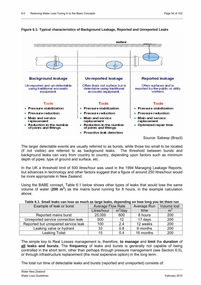
6.0 Reducing Water Loss:Tuning in to the Basic Concepts Page 50 of 102
Figure 6.1: Typical characteristics of Background Leakage, Reported and Unreported Leaks
Source: Sabesp (Brazil)
The larger detectable events are usually referred to as bursts, while those too small to be located (if not visible) are referred to as background leaks. The threshold between bursts and background leaks can vary from country to country, depending upon factors such as minimum depth of pipes, type of ground and surface, etc. In the UK a threshold limit of 500 litres/hour was used in the 1994 Managing Leakage Reports, but advances in technology and other factors suggest that a figure of around 250 litres/hour would be more appropriate in New Zealand. Using the BABE concept, Table 6.1 below shows other types of leaks that would lose the same volume of water (200 m3) as the mains burst running for 8 hours, in the example calculation above.
Table 6.1: Small leaks can lose as much as large leaks, depending on how long you let them run Average Flow Rate Volume lost Example of leak or burst
Litres/hour m3/day Average Run
time m3
Reported mains burst 25,000 600 8 hours 200 Unreported service connection leak 500 12 17 days 200
Reported but unrepaired service leak 100 2.4 12 weeks 200 Leaking valve or hydrant 33 0.8 8 months 200
Leaking Toilet 15 0.4 16 months 200 The simple key to Real Losses management is, therefore, to manage and limit the duration of all leaks and bursts. The frequency of leaks and bursts is generally not capable of being controlled in the short term, other than perhaps through pressure management (see Section 6.5), or through infrastructure replacement (the most expensive option) in the long term. The total run time of detectable leaks and bursts (reported and unreported) consists of:
Water New Zealand Water Loss Guidelines February 2010

6.0 Reducing Water Loss:Tuning in to the Basic Concepts Page 51 of 102
•• Awareness – from when a leak starts, until the Water Supplier becomes aware of it •• Location – the time then taken to locate the leak •• he leak
the absence of night flow measurements, it can be difficult to estimate Awareness times. But all
nce a Water Supplier for a medium or large system starts to record numbers of leaks and
UBL (litres/hour) = (20 x Lm + 1.25 x Nc) x (P/50)
here Lm is mains length (km). Nc is number of service connections (main to property line) and P
ation for a New Zealand Water Supplier (2000)
Repair – the time then taken to repair or shut off t InWater Suppliers should keep reliable records on their Location and Repair times, for every type of leak, as long running leaks with low flow rates are the largest source of annual Real Losses. Obursts, and location and repair times, in a format suitable for Component Analysis calculations, it should be possible within a couple of years to prepare a draft Component Analysis of Real Losses, as in Table 6.2, for comparison with the Real Losses assessed from the Water Balance. Unavoidable Background Leakage (UBL) up to the property line is calculated from an IWA formula (Ref 23):
1.5
wis the Average Zone Night Pressure (metres)
Table 6.2: BABE Component Analysis Calcul
.3 Active Leakage Control, with and without Night Flows and District Metering
ctive Leakage Control. When a Water Supplier only repairs leaks and bursts that are reported
he rate at which such unreported bursts accumulate (known as ‘Rate of Rise’, Refs 17 and 18)
ctive Leakage Control consists of managing the duration of unreported leaks by looking for
he simplest, but most labour intensive method of ALC is to sound every mains fitting and stop
6 Ato them, that is known as Passive Leakage Control. However, almost all distribution systems experience some leaks and bursts that are not reported. The activity of looking for, finding and repairing such unreported bursts is known as Active Leakage Control (ALC), and it is the ‘Easterly’ arrow of the 4 Components approach to managing Real Losses (Figure 5.6). Tvaries widely from one system to another, and even within parts of the same systems, depending upon factors such as whether the ground is surfaced or not, the type of soil and underlying rocks, the infrastructure condition, pressure and seasonal factors. Even where rates of rise are small, by international standards, if no ALC policy is in place, the component of real losses from unreported leaks will rise continuously, and will result in annual real losses that increase year on year, and gradual increases in Real Losses performance indicators. Athem, finding and repairing them. Although a small proportion of unreported leaks may be visible (usually in inaccessible locations), most unreported leaks do not surface, and have to be detected by sonic means. Ttap, or to use correlators and noise loggers, to investigate any sounds that indicate the presence of leaks. Typical costs for an experienced Contractor to do this type of survey are around $NZ 200 per km of mains. This could be a suitable approach for an initial sweep of a medium or large system that has an ILI that is within WBI Bands B, C or D, and has had no ALC activity for several years. Water New Zealand Water Loss Guidelines February 2010

6.0 Reducing Water Loss:Tuning in to the Basic Concepts Page 52 of 102
Water New Zealand Water Loss Guidelines February 2010
ight Flow Measurements: for small systems, and for medium or large systems that can be split
countries such as New Zealand, night flows can vary seasonally to a significant extent. Figure
Figure 6.2: Annual daily inflows (red) and night flows (blue) in a large DMA in Victoria
such nts
hilst it is preferable to have continuous metering at treatment works outlets and bulk supply
Zone inflows can be measured continuously for several days, the flow profile will give the first
Figure 6.3: Daily flow profile, high leakage Zone Figure 6.4: Daily flow profile, low leakage Zone
Ninto Zones, night flow measurements are an excellent way of identifying whether there are likely to be any unreported leaks worth looking for. This topic is covered in Appendix A. The following is a brief overview. In6.2 shows the annual pattern of daily system inflows, and night flows, in a large DMA (8000 service connections) in Victoria, Australia. Clearly, any attempt to estimate Real Losses from night flows during the summer is going to be invalidated by the large and unknown amount of exceptional night use due to garden watering, late night holiday activities, etc.
In circumstances, it is clearly preferable to measure and interpret night flow measuremeat times of the year when exceptional night use is at a minimum – typically April to October in New Zealand. Wpoints, a comparatively low cost but reasonably effective ALC policy can be commenced by creating temporary metering facilities in small systems (for example, by insertion meters) and taking inflow and pressure measurements for several consecutive nights, one or twice a year, around May and September (an Italian example is given in Ref. 17). Ifclue as to whether unreported leakage is high, or has risen since the previous measurements. If the night flow is a large proportion of the average daily flow, as in Figure 6.3, then there is likely to be substantial unreported (or unrepaired) leakage. However, if the night flow is only a small proportion of the average daily flow, as in Figure 6.4, then the likelihood of substantial unreported (or unrepaired) leakage is small.
0
2
4
6
8
10
12
14
1 136 271 406 541 676 811 946 1081 1216 1351 1486 1621 1756 18910
1
2
3
4
5
6
1 133 265 397 529 661 793 925 1057 1189 1321 1453 1585 1717 1849

6.0 Reducing Water Loss:Tuning in to the Basic Concepts Page 53 of 102
If it is only possible to obtain a [single] small number of night flows, once or twice a year, the
or Pressure Management Zones or District Metered Areas with continuous night flow
here is as yet no IWA standard terminology for components of night flow, and the fact that some
Figure 6.5: A practical terminology for components of minimum night flows in New Zealand
approach outlined in Sections 5.2 and 5.4 could be used to obtain a ‘Snapshot’ night leakage rate, then (if Average Zone Night Pressure is known) convert it to a ‘Snapshot ILI’ and WBI Band. Fmeasurements, a more systematic approach to analysis of night flows is recommended, which considers the night flow as a series of components of consumption and leakage, some of which are pressure-dependent. Tresidential properties in New Zealand are metered, and some are not, is an added complication. However, Figure 6.5 (from an early version of the ALCCalcs software, Ref. 18) shows a suitable practical terminology that New Zealand Water Suppliers are recommended to use, in the interests of standardising terminology. Some of the components of night flow are pressure-dependent, as indicated at the right-hand side of Figure 6.5; the FAVAD concept is explained in Section 6.4.
Source: ALCCalcs software
istrict Metered Areas: For medium and large systems, where there are a number of Zones with
he IWA Water Loss Task Force ‘DMA Guidance Notes’ (Ref 24, 2007) is a comprehensive and
Dcontinuous night flow measurements, these may be ‘District Metered Areas’ (DMAs) or ‘Pressure Managed Zones’ (PMZs). Tfree source of information on DMAs, aimed at leakage practitioners who have little or no experience of leakage control using DMAs. It covers: •• Philosophy of leakage control by DMA management •• Scheme design and DMA design •• Establishment of DMAs •• detection Selecting DMAs for leak •• Problematic DMAs •• hy Glossary and Bibliograp•• Night-Day Factors, Estimating Average Pressure, Selecting
he following brief notes on District Metered Areas are substantially sourced from the IWA Water
individual networks’ hydraulic and water quality onditions and regulations. Typically the design would commence from the trunk mains and
extend towards the distribution network. The objective is to separate as much as possible the
6 Appendices: Estimating DMAs for ALC, Night Consumption Estimation (UK experience), the BABE Concept, and Examples of successful DMA implementation.
TLoss Task Force DMA Guidance Notes (Ref. 24)
he design of DMA schemes is very specific to Tc
Water New Zealand Water Loss Guidelines February 2010
6.0 Reducing Water Loss:Tuning in to the Basic Concepts Page 54 of 102
DMAs from the trunk system, thus improving the control of the former without affecting the flexibility of the latter. Consequently a key element of this initial review will be to determine local practice or legal requirements regarding flexibility of supply such as satisfying fire fighting capacity etc. In large and complex networks, DMA management should be introduced as part of an overall plan to monitor the flow from the main sources. In such situations, it might be preferable to divide the
etwork first into larger sectors to identify the leakiest parts of the network. These sectors can
roject and its long-term efficiency. In fact, where ossible, natural boundaries should be used (rivers, streams and railway lines etc.) to limit the
below). The division of the network into PMZs nd DMAs facilitates the creation of a permanent pressure control system, thus enabling
nthen be prioritised for the creation of DMAs. This initial plan needs careful consideration to determine the boundaries, as this initial design will be crucial to the overall success of the ppnumber of valves to be closed. However in a complex network, particularly where the existing pressures are low, it is advisable to use a calibrated hydraulic network model to identify the hydraulic balance points. Small urban and rural networks tend to lend themselves more easily into DMAs, thus eliminating the need for sectors. Pressure control is an important factor in lowering and subsequently maintaining a low level of leakage in a water network (see also Section 6.6areduction of excess pressures, which: •• reduces the flow rates of any existing leaks (including undetectable background leakage) •• urring when existing detectable leaks have been repaired reduces the risk of new leaks occ•• prolongs the useful life of the distribution system ••
ible, into the reconfiguration of the system
inuous monitoring of inflows and pressures in PMZs and th reported and unreported large leaks, and rate
onsumption patterns, monitoring during operational alterations to supply, and monitoring
e need to optimise pressure management. In the UK, DMAs are often sized by the number of
owever, the consideration of Rate of Rise of unreported leakage comes into play here. If this
However where appropriate, large DMAs can be divided into smaller temporary DMAs by closing additional valves so that each sub-area is fed in turn through the DMA meter for leak detection
reduces some components of consumption Pressure control should be incorporated, wherever possduring the design of the DMA scheme. Most Utilities that operate District Metered Areas effectively on a continuous basis will tell of additional benefits that occur with cont
MAs, in addition to the rapid identification of boDof rise of smaller unreported leaks. These other benefits can be broadly summarised as ‘knowing what is happening in your system’ and include the identification of thefts of water, understanding daily, weekly and monthly cpressure fluctuations/performance of pressure reducing valves. There are various opinions on the sizing of District Metered Areas (DMAs). In practice, there will always be a significant variation in size of DMA due to the layout of the existing infrastructure and thproperties, where typically a property is supplied by a single customer connection. Consequently, DMAs in urban areas vary between 500 and 3000 service connections. It has been found that if a DMA is larger than 5000 properties, it becomes difficult to discriminate small bursts (e.g. service pipe bursts) from night flow data, and burst location takes longer. HRate of Rise is quite small (as in the large DMA in Figure 6.2, with 8000 service connections, an ILI close to 1.0 and a very low Rate of Rise of unreported leakage), the case for subdivision into smaller permanent DMA.s may be hard to justify purely on grounds of identifying unreported leaks.
Water New Zealand Water Loss Guidelines February 2010

6.0 Reducing Water Loss:Tuning in to the Basic Concepts Page 55 of 102
activities. In this case, the cost of any extra valves required should be taken into account at the DMA design stage.
Table 6.3: Indicative costs for water meter and pressure reducing valve installation
A typical installation of a water meter and pressure reducing valve is shown in Appendix H. Indicative costs for these types of installations are given in the table below:
Refer Appendix H for Typical Installation Details
Indicative Cost for Indicative Cost for 100mm Pipeline (as
Appendix H) 150mm Pipeline (as
Appendix H) 80mm PRV, Meter, 100mm PRV, Meter,
Strainer Strainer
Two chambers with lids, drainpipes etc 12,000 12,000
Pipes s bypass)
, fittings and line valves (exclude 3,000 6,000
Pressure Reducing Valve 2,300 3,000
Water Meter 1,200 1,500
Strainer 400 500
Total $ 18,900 $ 23,000
Note: Costs in 2009 NZ$
Setting Leakage Targets for Zones, and Bu mic Interv
etting Leakage Targets for Zones: for distribution systems with more that 20 service ins (which probably comprise most New Zealand distribution systems)
e majority of unreported leakage is likely to be associated with service connections, and so d leakage is
und to be on mains, then the target could be set in litre/km of mains/hour. However, these
6.4
dgeting for Econo ention
Sconnections per km of mathsimple targets can be set in litres/service connection/hour. If the majority of unreportefosimple indicators take no account of system pressure. Figure 6.14, in Section 6.6, shows how minimum night flow in a relatively high leakage Zone in Brazil changes significantly with pressure. The Unavoidable Annual Real Losses (UARL), which is used to calculate the Snapshot ILI from minimum night flows (see Section 5.4) increases: •• as the Average Zone Night Pressure (AZNP) increases ••
calculated from the equation:
= (0.75/DC + 0.0333) x AZNP
igure 6.6 shows that the UARL in litres/service connection/hour can vary widely, from:
as the density of connections (DC) increases.
he UARL in litres/service connection/hour can beT
UARL (litres/connection/hour) = (18/DC + 0.8) x AZNP/24 F •• 1.5 litres/connection/hour at 80 connections/km and 30 metres pressure, to •• 10 litres/connection/hour at 10 connections/km and 80 metres pressure
Water New Zealand Water Loss Guidelines February 2010
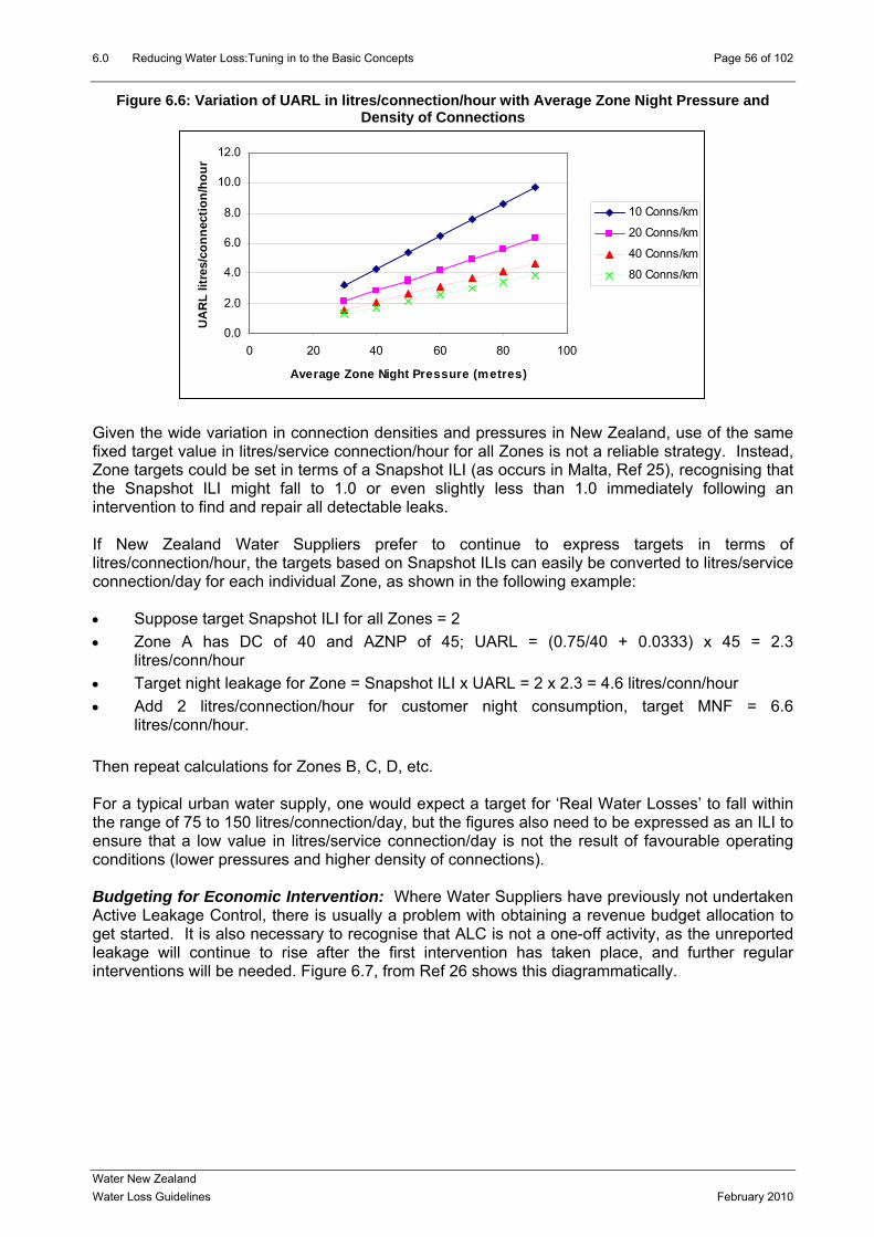
6.0 Reducing Water Loss:Tuning in to the Basic Concepts Page 56 of 102
Figure 6.6: Variation of UARL in litres/connection/hour with Average Zone Night Pressure and Density of Connections
0.0
2.0
4.0
6.0
8.0
10.0
12.0
0 20 40 60 80 100
Average Zone Night Pressure (metres)
UA
RL
litre
s/co
nnec
tion/
hour
10 Conns/km
20 Conns/km
40 Conns/km
80 Conns/km
Given the wide variation in connection densities and pressures in New Zealand, use of the same fixed target value in litres/service connection/hour for all Zones is not a reliable strategy. Instead, Zone targets could be set in terms of a Snapshot ILI (as occurs in Malta, Ref 25), recognising that the Snapshot ILI might fall to 1.0 or even slightly less than 1.0 immediately following an intervention to find and repair all detectable leaks. If New Zealand Water Suppliers prefer to continue to express targets in terms of litres/connection/hour, the targets based on Snapshot ILIs can easily be converted to litres/service connection/day for each individual Zone, as shown in the following example: •• Suppose target Snapshot ILI for all Zones = 2 •• Zone A has DC of 40 and AZNP of 45; UARL = (0.75/40 + 0.0333) x 45 = 2.3
litres/conn/hour •• Target night leakage for Zone = Snapshot ILI x UARL = 2 x 2.3 = 4.6 litres/conn/hour •• Add 2 litres/connection/hour for customer night consumption, target MNF = 6.6
litres/conn/hour. Then repeat calculations for Zones B, C, D, etc. For a typical urban water supply, one would expect a target for ‘Real Water Losses’ to fall within the range of 75 to 150 litres/connection/day, but the figures also need to be expressed as an ILI to ensure that a low value in litres/service connection/day is not the result of favourable operating conditions (lower pressures and higher density of connections). Budgeting for Economic Intervention: Where Water Suppliers have previously not undertaken Active Leakage Control, there is usually a problem with obtaining a revenue budget allocation to get started. It is also necessary to recognise that ALC is not a one-off activity, as the unreported leakage will continue to rise after the first intervention has taken place, and further regular interventions will be needed. Figure 6.7, from Ref 26 shows this diagrammatically.
Water New Zealand Water Loss Guidelines February 2010

6.0 Reducing Water Loss:Tuning in to the Basic Concepts Page 57 of 102
nents of Real Losses withFigure 6.7: Variation of Compo Time and ALC Interventions
0.5 1 1.5 2Time (years) -------->
Leve
l of l
eaka
ge --
------
-->
Background leakage
Unreported leakage
Unreported leakage
Reported leaks and bursts
SourceL Fantozzi & Lambert (2007)
If the Rate of Rise of unreported leakage (the slope of the grey triangles in Figure 6.7) can be estimated, even approximately, then the Economic Intervention frequency occurs when the $ value of the lost water in the grey triangle equals the cost of the intervention (CI) to detect the
e (RR) in m3 per day, per year:
unreported leaks. This Economic Intervention Concept (Refs. 17, 26) can then be used to assess the economic frequency of intervention, and the annual budget requirements for each Water Supplier (excluding repair costs). There are 3 quick methods for assessing Rate of Ris •• for Water Suppliers not currently doing ALC:
o increase in annual System Real Losses from successive annual water balances ••
o increase in night flows from one Spring or Autumn to the next
n are:
for Water Suppliers currently doing ALC or measuring night flows: o analysis of leaks found between successive interventions
he 2 other parameters needed for the calculatioT
•• Cost of an Intervention CI : in $, or $/service connection, or $/km of mains ••
3 3
.......(4)
A simple calculation for a system with 10,000 service connections and 250 km of mains is shown below: •• unreported leakage rises (RR) by 200 m3/day in a year (20 litres/connection/day/year) •• variable cost of Water CV = 0.5 $/m3 •• cost of a whole system intervention CI (excluding repairs) = $200/km = 200 x 250 = $50,000
Variable Cost of lost water CV : $/m3 If Intervention Cost CI is in $, Variable Cost CV is in $/m and RR is in m /day, per year: Economic Intervention Frequency EIF (months) = √(0.789 x CI/(CV x RR)) .....................(1) Economic Percentage of system to be surveyed annually EP (%) = 100 x 12/EIF............(2) Annual Budget for Intervention (excluding repair costs) ABI ($) = EP% x CI.....................(3) Economic Unreported Real Losses EURL (m3) = ABI/CV ..........................................
Water New Zealand Water Loss Guidelines February 2010

6.0 Reducing Water Loss:Tuning in to the Basic Concepts Page 58 of 102
Economic Intervention Frequency (months) = √(0.789 x CI/(CV x RR)) = 20 months Econom
nnual Budget for Intervention (excluding repair costs) ABI ($) = EP% x CI = $30,000/year (equivalent to $3/service conneEconomic Unreported Real Losses EU m3/year (16 litres/conn/day) The ALCCalcs software (Ref. 18) is designed for these calculations, and the same calculation as done manually above is shown in Figure 6.8, with confidence limits.
Figure 6.8: Calculation of Economic Intervention Parameters using ALCCalcs software
ic Percentage of system to be surveyed annually EP (%) = 100 x 12/EIF = 60% A
ction/year) RL (m3) = ABI/CV = 60,000
This approach uses the same basic methodology as the more complex methods developed in the
K during the 1990’s, as can be seen from Figure 6.9, which is one of the graphs produced with ate of R, CI eters
Uthe ALCCalcs calculations in Figure 6.8. However, it is much easier to apply using the ‘RRise’ concept. Because the predictive equations are based on square root functions of Rand CV, the results are not highly sensitive to moderate variations in estimating these param(particularly Rate of Rise, RR).
Water New Zealand Water Loss Guidelines February 2010
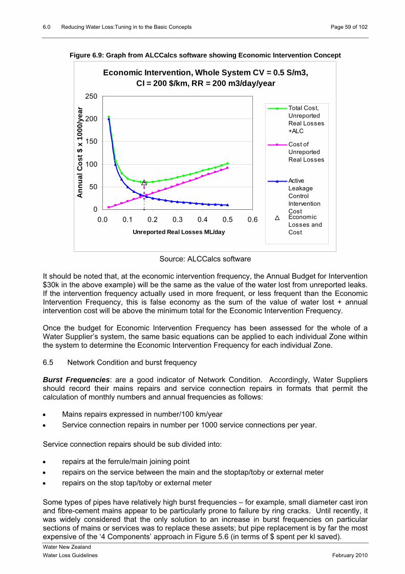
6.0 Reducing Water Loss:Tuning in to the Basic Concepts Page 59 of 102
Figure 6.9: Graph from ALCCalcs software showing Economic Intervention Concept
Economic Intervention, Whole System CV = 0.5 S/m3,
0
50
100
150
0.0 0.1 0.2 0.3 0.4 0.5 0.6
Unreported Real Losses ML/day
Ann
ual C
ost $
x 1
000/
year
CI = 200 $/km, RR = 200 m3/day/year250
Total Cost,Unreported
+ALC
200Real Losses
Cost ofUnreportedReal Losses
ActiveLeakageControlInterventionCostEconomicLosses andCost
Source: ALCCalcs software
It should be noted that, at the economic intervention frequency, the Annual Budget for Intervention $30k in the above example) will be the same as the value of the water lost from unreported leaks. If the intervention frequency actually used in more frequent, or less frequent than the Economic Intervention Frequency, this is false economy as the sum of the value of water lost + annual intervention cost will be above the minimum total for the Economic Intervention Frequency. Once the budget for Economic Intervention Frequency has been assessed for the whole of a Water Supplier’s system, the same basic equations can be applied to each individual Zone within the system to determine the Economic Intervention Frequency for each individual Zone. 6.5 Network Condition and burst frequency Burst Frequencies: are a good indicator of Network Condition. Accordingly, Water Suppliers should record their mains repairs and service connection repairs in formats that permit the calculation of monthly numbers and annual frequencies as follows: •• Mains repairs expressed in number/100 km/year •• Service connection repairs in number per 1000 service connections per year. Service connection repairs should be sub divided into: •• joining point •• repairs on the service between the main and the stoptap/toby or external meter •• repairs on the stop tap/toby or external meter Some types of pipes have relatively high burst frequencies – for example, small diameter cast iron and fibre-cement mains appear to be particularly prone to failure by ring cracks. Until recently, it was widely considered that the only solution to an increase in burst frequencies on particular sections of mains or services was to replace these assets; but pipe replacement is by far the most expensive of the ‘4 Components’ approach in Figure 5.6 (in terms of $ spent per kl saved).
repairs at the ferrule/main
Water New Zealand Water Loss Guidelines February 2010

6.0 Reducing Water Loss:Tuning in to the Basic Concepts Page 60 of 102
Howeve clearly identified many Zones world-wide (Ref 12, 2006) where burst frequencies on mains and or service connections have been significantly reduced by pressure management. This has resulted in an international resurgence of interest in pressure management – which previously tended to be cost-justified only on the value of the reduction in leak flow rates. When pressure management is introduced, in some Zones both mains and service bursts are reduced (see Fig 2.5). In other Zones, either mains or service bursts are reduced, but not both. The latest WLTF Pressure Management Group method for predicting if either, or both, or neither, will reduce is outlined in Appendix D. The starting point is to compare actual repair frequencies (for, say two years prior to possible implementation) with the reference frequencies for well managed infrastructure in the UARL formula of: •• 13 per 100 km /year for mains repairs •• 3 per 1000 service connections/year for services (excluding stop taps/tobys, meter repairs) Separate values of a Burst Frequency Index (BFI) can then be calculated for mains, and for services. For example, in Wide Bay Water (Australia) (Figures 6.10 and 6.11), before implementation of pressure management, the mains burst frequency was around 12 to 15 per 100 km/year, close to the UARL frequency of 13 per 100 km/year; but the service pipe burst frequency was 31 to 34 per 1000 service connections/year (around 11 times the UARL frequency of 3 per 1000 service connections/year).
Figure 6.10: Mains burst frequencies Figure 6.11 Service connection burst frequencies
r, the Pressure Management Group of the IWA Water Loss Task Force has now
02468
1012
Fre
141618
1999-200
02000
/2001
2001/200
22002
/2003
2003/200
42004
/2005
2005/200
6
quency
/100 km
/year
ActualUARL figure
05
25
Fre
303540
101520
quency
/ 1000 c
onns/ye
ar
1999-200
02000
/2001
2001/200
22002
/2003
2003/200
42004
/2005
2005/200
6
edictor that, with pressure management, for mains was
lso a good indicator that mains burst frequency would hardly be affected by the pressure
eduction is under ongoing review by the Pressure as reliable
ne of the immediate practical benefits of reductions in burst frequencies is that some resources
The high BFI for service connections was a good prservice connection bursts would reduce significantly (which they did). The low BFI amanagement. A quantitative prediction method of bursts rManagement Group of the Water Loss Task Force, and is being tested and improveddata increasingly becomes available (Ref. 13). Oin operational budgets for repairs costs, out of hours work costs, manpower etc are immediately freed up for other uses
Water New Zealand Water Loss Guidelines February 2010

6.0 Reducing Water Loss:Tuning in to the Basic Concepts Page 61 of 102
Although mains burst frequencies in Fig. 6.10 did not change significantly (because they were in good condition as indicated by their BFI being close to 1), the prediction method in Appendix D
plies that their working life will have been increased. A methodology to value this benefit is
s ressures, eliminating transients and faulty level controls all of which cause the distribution
imcurrently being investigated by the Pressure Management Group of the Water Loss Task Force. 6.6 The many influences of Pressure Management Pressure Management has been defined (Ref 12) as The practice of managing system pressures to the optimum levels of service ensuring sufficient and efficient supply to legitimate uses and consumers, while reducing unnecessary or excespsystem to leak unnecessarily Pressure management has the following benefits: •• reduction of existing and future leak flow rates, and some components of consumption •• cy, and/or extension of infrastructure life
igure 6.12 (which can be compared with Figure 6.7) shows how implementing of pressure
possible reduction of new burst frequen Fmanagement can be effective in reducing all the components of Real Losses.
Figure 6.12: Influence of Pressure Management on Components of Real Losses <- BEFORE PRESSURE MANAGEMENT -><-------------- AFTER PRESSURE MANAGEMENT ----------------------->
0.5 1 1.5 2 2.5 3 3.5 4 4.5 5Time (years) -------->
Leve
l of l
eaka
ge --
------
-->
Background leakageBackground leakage
Unreported leakage
Unreported leakage
Unreported leakage
Unreported leakage
Frequency and flow rates of reported leaks reduceRate of rise of unreported leakage reduces
Frequency and cost of economic intervention reducesBackground leakage reduces
Reported leaks and bursts
Source: Fantozzi and Lambert, 2007
All of these influences can now be predicted, with increasing reliability (Ref. 13). Predicting changes in leak flow rates The most ‘Best Practice’ form of equation for pressure: leak flow rate relationships is based on a simplified version of the FAVAD (Fixed and Variable
rea Discharges) concept (Ref. 27), using the equation:
gure 6.13 if the average pressure is reduced from P0 to P1, flow rates through
A
Leak flow rate L varies with PN1 and L1/L0 = (P1/P0)N1
s shown in FiAexisting leaks change from L0 to L1, and the extent of the change depends on the ratio of average pressures and the exponent N1. Higher N1 values represent leaks where flow rate is more sensitive to pressure.
Water New Zealand Water Loss Guidelines February 2010

6.0 Reducing Water Loss:Tuning in to the Basic Concepts Page 62 of 102
Figure 6.13: FAVAD Equation shown as a graph
0.00
0.20
1.40
1.20 L 1/L
o
1.00
Ra
te
0.40
0.60
0.80
o o
f L
eaka
ge
s
N 1 = 0 .50
N 1 = 1 .00
N 1 = 1 .15
N 1 = 1 .50
N 1 = 2 .50
Ra
ti
0.00 0.10 0.20 0.30 0.40 0.50 0.60 0.70 0.80 0.90 1.00 1.10 1.20
R a tio o f P res su re s P 1/P o
Source: PressCalcs software
Tests on systems and pipe samples have shown that different kinds of leaks have different N1 exponents: •• for background leakage, and splits on flexible pipes, N1 is usually close to 1.5 •• for detectable leaks and bursts on rigid pipes (corrosion holes, ring cracks etc) N1 = 0.5
Figure 6.14 from Brazil, shows an N1 test. When night flow stabilises, pressure is reduced in steps, and the night flow reduces with each step. After deducting estimates for night consumption, the three night leakage rates can be compared with the three Average Zone Night Pressures, and the N1 values calculated.
Figure 6.14: Example of an N1 Test (Brazil). Pressure in red, night flow in blue
Experimentos - Relacao dentre Vazao e Pressao
450 50
0
200
400
0:00
0:25
0:50
1:15
1:40
2:05
2:30
2:55
3:20
3:45
4:10
4:35
5:00
5:25
5:50
6:15
6:40
7:05
7:30
7:55
8:20
8:45
9:10
9:35
10:00
10:25
10:50
11:15
11:40
Hora
Vaza
o M
3/ho
ra
0
5
25
30
35
45
mca
300
35040
250
50
100
150
10
15
20
Water New Zealand Water Loss Guidelines February 2010
Flowrate m3/hr Pressure m

6.0 Reducing Water Loss:Tuning in to the Basic Concepts Page 63 of 102
Drawing on a internationa nt Team has developed and tested the prediction d Figure 6.15, the upper line for 100% flexible pipe materials (p = 0%) is assumed to be constant at 1.5, whatever the ILI. The lower line for 100% rigid pipe materials was calculated assuming N1 = 1.5 for unavoidable background leakage for infrastructure in good condition, and N1 = 0.5 for detectable leaks in rigid pipes. Intermediate lines are based on the empirical equation:
N1 = 1.5 – (1 – 0.65/ILI) x p/100 So, for example, if ILI = 1.3 and p = 43%, the predicted N1 is around 1.3.
Figure 6.15: Predicting the N1 exponent using ILI and % of detectable real losses on rigid pipes
l test data, the IWA WLTF Pressure Managememethod for N1 shown in the equation below, an
Power Law Exponent N1 vs ILI: p = % of detectable real losses on rigid pipes
0.0
0.2
Pow
0.4
0.6
0.8
1.0
1.2
1.4
1.6
0 1 2 3 4 5 6 7 8 9 10
er L
aw E
xpon
ent N
1
p=0%
p=20%
p=40%
p=60%
p=80%
p=100%
Infrastructure Leakage Index ILI
Predicting changes in some components of residential consumption also uses the Favad concept, but with an exponent N3. The consumption is split into ‘in-house’ and ‘outside’ components. for ‘Outside’ components, N3 is 0.5 •• for hoses and sprinklers, 0.75 for seepage and weeper
hoses, and (obviously) zero for swimming pools. •• For ‘in-house’ consumption, N3 is less (usually in the range 0 to 0.1) and depends upon a
his method is used to predict changes in income from metered customers. Note that, if a Water upplier is considering introducing Pressure Management and metering residential customers for e first time, there is merit in doing the pressure management first as there will be no significant
hange in income if residential consumption reduces.
redicting changes in burst frequencies has been explained in Section 6.5 and Appendix D. owever, there is one simple test that every Water Supplier should do. The largest reductions in
management have been associated with pumped systems, with pressure ansients, which can add 20 or 30 metres to normal maximum pressures.
r the presence of pressure transients and surges in all Zones, even those supplied by ravity. This is because customers are sometimes the cause of transients (pumps switched on nd off, sudden closures of valves).
et a pressure logger somewhere in the Zone for 1 week, recording at 1 second intervals. The sults can sometimes be surprising (Figure 6.16), as most pressure loggers are set to record the
average pressure over 5, 10 or 15 minutes, and would not show the presence of transients.
number of specific factors TSthc PHbursts from pressure tr So check foga Sre
Water New Zealand Water Loss Guidelines February 2010
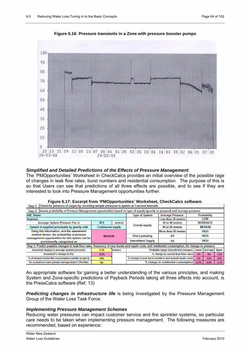
6.0 Reducing Water Loss:Tuning in to the Basic Concepts Page 64 of 102
Simplified and Detailed Predictions of the Effects of Pressure Management: The ‘PMOpportunities’ Worksheet in CheckCalcs provides an initial overview of the possible rage of changes in leak flow rates, burst numbers and residential consumption. The pur ose of this is o that Users can see that predictions of all three effects are possible, and to see if they are
Figure 6.16: Pressure transients in a Zone with pressure booster pumps
psinterested to look into Pressure Management opportunities further.
Figure 6.17: Excerpt from ‘PMOpportunities’ Worksheet, CheckCalcs software.
An appropriate software for gaining a better understanding of the various principles, and making System and Zone-specific predictions of Payback Periods taking all three effects into account, is the PressCalcs software (Ref. 13) Predicting changes in infrastructure life is being investigated by the Pressure Management Group of the Water Loss Task Force.
plementing Pressure Management Schemes ImReducing water pressures can impact customer service and fire sprinkler systems, so particular care needs to be taken when implementing pressure management. The following measures are recommended, based on experience:
Water New Zealand Water Loss Guidelines February 2010

6.0 Reducing Water Loss:Tuning in to the Basic Concepts Page 65 of 102
• Identif er or not the
l
argue cost of
term
The atic in of fire
• when to all
. other
• d after
•
showers (which are an essential customer requirement), as some showers will be
6.7 Eco Economic level of leakage (ELL) was a concept mainly developed in England and Wales during the period 1994 to 1998. The Water Companies – many of which had been privatised in 1990 – were required to demonstrate to the Economic Regulator (OFWAT – Office of Water Services - that they had achieved economic leakage levels, using ‘robust’ methodologies. The basics of the two main methodologies used first appeared in one of the 1994 UK Leakage Control Initiative Reports (Ref. 28). Both methods were based on the concept of minimising the sum of Cost of Intervention and Cost of Lost Water, and were mainly concerned with assessing the Economic Intervention Frequency for Active Leakage Control (the right hand arrow of the 4 Components diagram), see Figure 6.9. One approach was based on modelling of BABE omponents, the other was an empirical curve fit to night flows. Neither could be easily applied at
Companies had demonstrated, to the satisfaction of OFWAT, at they had achieved Economic Leakage levels. The ILIs for England and Wales Companies in
ILIs range from 1.3 to 3.3, and:
y fire sprinkler systems in the area to be affected, and establish whethsystems are likely to be non-compliant after the pressure reduction. Depending on the policy of the Water Supplier, the response to property owners can range from ‘our legaopinion is that there is no obligation to maintain water pressures above a minimum servicelevel (of between 200kPa and 300kPa)’, to the Water Supplier working proactively with theproperty owner and fire contractor to resolve issues before they arise. The latter is considered to be a responsible approach and is recommended. A customer can that if the Water Supplier is implementing these measures to reduce costs, then the making initial changes should be considered in a cost/benefit analysis (i.e. the longsavings should justify initial costs). The cost of installing pumps for fire sprinkler systemsis high (typically more than $60,000 with diesel backup power supply) and hence the initial assessment of sprinkler systems should be carried out at an early planning stage. issue of fire sprinkler system compliance is likely to be the most problemimplementing pressure management, and options for areas with a high density sprinkler systems may be limited.
A communications strategy is necessary, as customers will notice changes pressures are adjusted. This typically comprises public notices and a letter dropproperty owners advising of the changes and the benefits of pressure managementSome impacts, such as the performance of hydraulic disabled person lifts, or hydraulically operated equipment are often difficult to pre-empt.
Monitoring of pressures in the network immediately before, during the transition, anadjusting pressures is essential.
Pressures should be reduced gradually and in stages over a number of days or weeks sothat impacts can be dealt with in a managed way. A plumber should be on hand to adjust
adversely affected. Further useful information on implementing pressure management is included in the paper by Pilipovic and Taylor (2002) entitled ‘Pressure Management in Waitakere City – A Case Study’, a copy of which is provided in Appendix I.
nomic level of leakage
c both System and Zone level. By 1998, most England and Walesth2002 are shown in Figure 6.18. All but the two Companies with the highest ILIs are considered to have achieved Economic Leakage Levels. Their •• water is scarce and relatively expensive Companies with the lowest ILI are those where•• Companies with the lowest ILI are those where water is more plentiful and relatively cheap.
Water New Zealand Water Loss Guidelines February 2010

6.0 Reducing Water Loss:Tuning in to the Basic Concepts Page 66 of 102
Figure 6.18: ILIs for England & Wales Water Companies, 2002-03
A b adeveloplentifuclose to
in Figure 6.19, th evere drought, a majority of Australian Utilities (including all the
e c se to 1, but that a few (mostly in the wetter North and North-
e Report (Ref.
Source: UK Environment Agency
ro d provisional conclusion to be drawn from this England and Wales data is that in a ped country, Economic ILIs of up around 3 are roughly appropriate for a Water Utility with l and cheap supplies, but where there are shortages and water is scarce, ILIs should be 1.0.
Recent experiences in Australia and New Zealand also suggest that, where water is scarce (or potentially scarce) and therefore expensive, Water Suppliers should be achieving ILIs close to 1.
Is from the 2007-08 Australian National Performance Report (Ref 29), shownILshow at, following five years of s
rg ities) are achieving ILIs clolaEast) have ILIs around 3. Several of the lowest ILIs have been checked and found to be under-estimates, due to problems of measuring such low levels of leakage (many of which have been discussed in Sections 3 and 4 of these Guidelines).
he Real Losses in most Australian that provide data to the National PerformancT29) are now so low that the new WSAA Water Balance software (Ref. 14), has split WBI Band A into two – Band A1, for ILI less than 1.5, and Band A2, for ILIs 1.5 to 2.
Water New Zealand Water Loss Guidelines February 2010

6.0 Reducing Water Loss:Tuning in to the Basic Concepts Page 67 of 102
Figure 6.19: ILIs in Australian Water Utilities, 2007-08
conomic Intervention Frequency for Active Leakage Control at current pressures, and then to
ater Suppliers whose data and practices are bust enough for such analysis at present. So the emphasis for the next few years should be to
.8 Key points from Section 6 •• Section 6.1 and Appendix G provide an overview of Bulk Metering and associated problems •• reported mains bursts usually account for less than 10% of Annual Real Losses •• the basic principles of Component Analysis of Real Losses, using the BABE (Bursts and
Background Estimates) concept assist understanding of how and where real losses occur •• real loss management deals with limiting the duration of all leaks, however small
o a toilet leaking for 16 months can lose as much water as a reported mains burst •• all Water Suppliers need to do Active Leakage Control (looking for unreported leaks), at a
frequency appropriate to their system characteristics •• night flow measurements in Zones are an excellent way of identifying whether there are any
unreported leaks worth looking for o but take measurements at times when night consumption is at its lowest
In New Zealand, in the greater Auckland region, where water is also relatively scarce and relatively expensive, most of the Distribution Utilities are now achieving ILIs in the range 1.0 to 1.5. Regarding the broader topic of assessment of Economic Leakage Levels, it is now very clear from the work of the IWA Water Losses Task Force that it is not sufficient to simply calculate anEclaim this is an Economic Leakage Level. It is also necessary to look for opportunities for pressure management, and to bring the effect of such activities into the calculations, as indicated in Figure 6.12. Software to do such calculations (ELLCalcs, Ref. 30) is being used in Canada (Ref. 31). However, in New Zealand, there are relatively few Wrounderstand and apply principles of Economic Intervention for Active Leakage Control, and to seek opportunities for Pressure Management with relatively short payback periods. 6
Water New Zealand Water Loss Guidelines February 2010

6.0 Reducing Water Loss:Tuning in to the Basic Concepts Page 68 of 102
•• a practical standard terminology for components of minimum night flows in New Zealand is proposed in Figure 6.5; please use it to reduce misunderstandings and wasted time
•• the IWA DMA manual (Ref 24) is an excellent source of information on setting up DMAs •• unavoidable real losses vary widely with average pressure and density of connections in
individual Zones; so use Snapshot ILI to set targets for night flow, and then express them in litres/connection/hour if you prefer
•• the Economic Intervention concept can be used to rapidly assess appropriate budgets for Active Leakage Control, giving the same results as more complex UK calculation methods
•• burst frequencies on mains (per 100 km of mains/year) and on service connections (per 1000 service connections/year) are a good indicator of network condition o and if the frequencies are high they may be reduced by pressure management
•• pressure management has other benefits – reduction of leak flow rates and some components of consumption - so there is advantage to undertaking pressure management before metering residential customers
•• all Zones should be checked for pressure transients – even Zones supplied by gravity •• a rapid overview assessment of possible range of benefits of pressure management can be
made with CheckCalcs •• the Pressure Management Group of the IWA Water Loss Task Force is progressing
improved methods of detailed predictions of pressure management benefits •• reducing water pressures can impact customer service and fire sprinkler systems so
particular care needs to be taken when implementing pressure management •• data from the UK suggests that economic ILIs are likely to be within the range 1 to 3, with
lowest values where water is most expensive and supply is actually or potentially limited ••
can be achieved experience from Australia and New Zealand (Auckland region) shows that ILIs close to 1
Water New Zealand Water Loss Guidelines February 2010

7.0 Recommended Water Loss Strategy Page 69 of 102
7.0 Recommended Water Loss Strategy
in achSupp t an advanced level.
A recommended water loss strategy is summarised in the table below. The order of the items in the left hand column of the table is the order which is generally likely to be the most cost effective
ieving reduction of Real Losses. The table describes typical activities required of Water liers operating at a basic level and a
Table 7.1: Recommended Water Loss Strategy
Activity Basic Advanced
Activtegte
le 2.1 ityor Size of
• Categorise your System(s) as Large, Medium or Small, using Tab•
1: Ca iseSys m
Identify the Recommended Method(s) for assessing Real Losses, either Water Balance and/or Minimum Night Flow Measurements
ActivBalan
P rfo
Leaka
confid
2008
ftw
f water
omer meter under-
Consumption, and customer meter under-registration.
limits for the following: urate
− For metered systems, meter
tage under-
out. − Unbilled Authorised
Consumption (system flushing etc.) is metered or assessed.
ity 2a: Water ce calculation
• Be aware of high uncertainty in main components o
• Reduced level of uncertainty
of Real Water balance such as system input, − System input meters accLosses and
e rmance authorised consumption and cust
(and preferably multiple).
Indicators, including Infrastructure
ge Index ILI,
registration. • For unmetered connections,
assumptions made regarding
lag effects carefully considered and Meter under-registration (accuracy
preferably with ence limits,
consumption, not based on any monitoring data, will have the
) checks have been carried out to justify percen
using BenchlossNZ or
largest uncertainty • Use standard defaults for
registration figure(s) used. − For unmetered systems, a
CheckCalcsNZ so are.
Unauthorised Consumption, Unbilled Authorised
soundly based ‘monitoring’ programme has been carried
Activity 2b: Minimum Night Flow measurements (MNF).
• Large open network. • Occasional datalogging. • Use of insertion flow meters. • Reservoir drop tests. • Assess the Snapshot ILI
• Network divided into District Metered Areas (DMAs).
• Calibrated water meters supplying DMAs.
• Continuous on-line monitoring. • Automatic reporting on MNF. • Economic Intervention Policy
Activity 3: Classify current performance using World Bank Institute Banding System
• Classify ILI or Snapshot ILI in WBI Band A, B, C or D using Figure 5.10
• Check appropriate Activity Priorities using Figure 5.11
• Classify ILI or Snapshot ILI in WBI Band A, B, C or D using Figure 5.10
• Check appropriate Activity Priorities using Figure 5.11
Activity 4: Investigate Speed and Quality of Repairs.
• Slow, random response to reported faults, including reported and unreported leaks.
• Failure to repair difficult leaks, smaller leaks on Utility system
• Failure to ensure leaks on unmetered private service pipes are repaired
• Monitored, timely response to all reported faults and unreported leaks on Utility infrastructure.
• Optimised resources for maintenance work.
• Options for improved maintenance, including methods and materials, are continually examined to reduce leakage volumes.
• Ensures leaks on unmetered
Water New Zealand Water Loss Guidelines February 2010

7.0 Recommended Water Loss Strategy Page 70 of 102
Activ y it Basic Advanced
private service pipes are repaired Activity 5: Active Leakage Control.
• Random interventions, usually after problems have occurred.
• Untargeted acoustic leak detection.
• Timely intervention if high MNFs develop quickly.
• Leak detection targeted in DMAs
• Use of basic technology
ported leaks with long run
with high MNF. • testing or splitting of
establish high leakage
frequency
(acoustic listening only). Use of step
zones to • Unre
times • No annual budget for regular
• Use of wide range of equipment acoustic listening sensors, noise
leak detection loggers including correlators. • Economic intervention
precincts.
and annual budget have beenestablished for network.
Activity 6: PreManagement.
ssure
• s
•
•
•
• ‘ade
• Usesectmodulating where appropriate.)
• Optinetw
at
frequency on mains and service conn
No assessment of average pressure in System and ZoneNo checks for pressuretransients
• Benefits of pressure management not understood or accepted Largely open network with no pressure zoning; excess pressure may be well above minimum standard of service.No use of pressure reducing valves or transient control.
Each DMA operating at quate’ but not excessive
pressure. of transient control, network orisation and PRVs (flow
mum pressure regime for ork –if not, further pressure
m nagement targeted at Zoneswith high leakage and high burs
ections.
Activity 7: Infrastructure Condition and Break
• gathered.
• Frequencies of repairs on mains calculated
rvice
if
• reco
• Break frequencies on m
eloped ation
t
Frequency.
No asset condition information
and mains fittings not • Frequency of repairs on se
connections not calculated ramme • Network renewal prog
any, randomly developed.
Network faults systematically rded.
ains, and on services, compared to international reference values
• Renewal programme devbased on condition informand network fault information.
d • Renewal policy developed anincluded in Asset ManagemenPlan.
Hence a recommende
Activity 1: Ca
d
tegoris e, Medium or Small using Table 2.1, and to inimum
y 2a: If doin is a pt using very basic assumption • identify deficie alan• use confidenc ess calculated Real Los• arrange for improvements (e.g. to bulk metering) if n• calculate real water loss KPIs, including Infrastruc
approach would be as follows:
e the Size of System as Largidentify whetherusing Activit
use Water Balance and/or M Night Flows to assess Real Losses
g a Water Balance - even if this s:
n approximate first cut attem
ncies in the data used for water be limits to ass
ce volumes ses volume and uncertainty ecessary
ture Leakage Index ILI
Water New Zealand Water Loss Guidelines February 2010

7.0 Recommended Water Loss Strategy Page 71 of 102
Activity 2b: If using Minimum Night Flows:
me t con app night c will be higher for
unmetered • remember t pressure• calculate the ding Snaps
Activity 3: Classify current Real Loss management p k Institute Banding S appropr 5.11 Activity 4: Investigate Speed and Quality of Repair issues,
L egular t flows – or
• if very limited adings in e• splitting of z to monitor water• set intervention targets in each supply area/zone, preferably based on economic
intervention • arrange for in hous
Activity 6: Pressure ou un f pressure management, and how pressure management mi anagement of your system.
ystems ( sure
w e.
• single feed va• little or no im• high burst fr • high leakage and high r eported • pressures at critical points in system substantially rd
of service
Activity 7: Review the condition of the network and renewal programmes, with particular on mains and services. Valve and hydrant
y.
• take the• deduct a
asurements at times of basic nighropriate estimate for customer
nsumption only onsumption (this
residential properties) o assess the average system real water loss KPIs, inclu
at the time the MNF is measured hot ILI
erformance using the World Baniate Activity Priorities using Figureystem (Figure 5.10), and check
and address deficiencies
Activity 5: Active either by telemetry
eakage Control: arrange for r regular use of a data logger.
monitoring of minimum nigh
budget, take overnight re arly Spring and late Autumn loss in smaller areas ones may be an option
active leak detection either using
Management: ensure that y
e resources or a contractor.
derstand the various benefits oght improve m
Check all s Consider reducing
including gravity systems) for pres transients.
ater pressures where this is feasibl Prioritise areas with:
and few (preferably zero) boundary lves pact on fire sprinkler systems
equencies (mains and/or services)ates of rise of unr leakage
in excess of the minimum standa
emphasis on reliable recording of burst frequencies condition assessment and renewal programmes may also be necessar
Water New Zealand Water Loss Guidelines February 2010

8.0 Resources Page 72 of 102
8.0 Resources It is the int ese Guidelines on a single ebobtain opi In the se le 8.1 below.
ention to assemble as many as possible of the References to th w site in New Zealand, which would be accessible free of charge to anyone wishing to c es.
ca of software mentioned in these Guidelines, copies may be obtained as shown in Tab
Table 8.1: Software and Associated Manuals
Manuals Functions Available From Benchmarking of Water Los2008)
Includes User Manual for Water New Zealand ses in New Zealand (Feb. BenchlossNZ2008V2a
WaVer
ter Loss Guidelines, sion 1a, February 2010
For planning ‘Next Steps; in managing Real Losses
Water New Zealand
Software Benc ssN2008)
ealand nual)
hlo Z2008V2a (Feb Water Balance and Performance Water New Ze ma Indicator Calculations (included with th
Chec alc
including Water Balance and PI
aland Water
Water Corporation/ILMSS
kC sNZV3a (Feb 2008) Check on Leakage and Pressure Free to New ZeManagement Opportunities, Utilities, from Wide Bay
Calculations Ltd PressCalcsV4a (Dec 2009) Explains concepts used to predict Wide Bay Water
influences of pressure management, with calculations
Corporation/ILMSS Ltd. Utility Site Licence
ALCCalcs V4b (Dec 2009) Explains concepts used to assess Economic Intervention
calculations
Wide Bay Water Corporation/ILMSS Ltd.
y Site Licence frequencies and budgets, with Utilit
ELL
ay Water
Utility Site Licence
Calcs V3a (June 2009) For calculation of Short-Run Economic Leakage Level, with
Wide BCorporation/ILMSS Ltd.
and without pressuremanagement
NLRx Night Wide Bay Water NDFCalcs Used for assessing Leakage Rate, Daily Real Losses Corporation/ILMSS Ltd. and Snapshot ILI from night flows Utility Site Licence
IWA P blicu ations DG
istrict Me s (DMA) u
200
Covers the design of DMAs, Available free from Water tered Areaidance Notes (February 7 Version 1)
analysis of flow measurement, prioritising of leak location from DMA data, management of DMAs, and case studies.
New Zealand website.
Pressure Management Guidance Notes – Due in late 2010
To be available free from Water New Zealand website.
Water New Zealand Water Loss Guidelines February 2010

9.0 References Page 73 of 102
9.0 References
ing ‘Manuals of Best Practice’ Series, 2000. ISBN 1 900222 272
and. (2002) NZWWA.
3. User Manual for B ZWWA
n New
NZWWA.
a s Loss and Pressure Management portunities, including Water Balance and PI calculations (Jan 2008). ILMSS Ltd /
r 8. Cabrera E, 2007 Settin
Efficiency. American Wa ociation Summer Meeting, Toronto, June 2007 .
9. OVGW W 63 (2009): Evaluation and Measures for Water Loss Reduction. – Directive of the Austrian
and 10. Performance Indicators H et al.
(June 2006). IWA Publishing 'Manuals of Best Practice' Series, ISBN 1843390515
11. A Review of PerformanLambert A et al. AQUA, D
J and Lamber
and reduces unnecessa 02007', Bucharest -Romania, 23-26 Sept 2007. ISBN 978-973-7681-24-9. Paper 51,
p 511-521.
s of management. ation
14. Water Balance software (2010). Updated Water Balance software for Water Services
/ILMSS Ltd/Wide Bay Water
Security of Supply, leakage and water efficiency 2005/06 ( Services (Ofwat) Report
16. Lambert A and Dr Hirner W (2000): Losses from Water Supply Systems: Standard
Terminology and Recommended Performance Measures (Oct 2000). IWA Blue Pages 17. Lambert, A.O and Lalonde, A.(2005). Using Practical Predictions of Economic
Intervention Frequency to calculate Short-run Economic Leakage Level, with or
1. Performance Indicators for Water Supply Services. Alegre Dr H et al, 2000. IWA
Publish 2. BenchlossNZ Version 1a software for Benchmarking of Water Losses in New
Zeal
enchlossNZ software Version 1a. (2002). N 4. BenchlossNZ Version
Zealand (Feb 2008). NZW 5.
2a software for Benchmarking WA
of Water Losses i
User Manual for the BenchlossNZ softw 6. CheckCalcsNZ V3
are Version 2a (Feb 2008).
oftware for Water OpWide Bay Water Corporat
ion
7. World Bank Institute (2005). NRW Training Module 6: Perfo
g and Using Performance Indicater Works Ass
mance Indicators
tors for Improving Utility
Water Losses in Water Supply Systems: Assessment,
Association for Gas Water (OVGW), Vienna, Austria.
for Water Supply Services, 2nd Edition. Alegre Dr
ce Indicators for Real Losses fro
ec 1999. ISSN 0003-7214 m Water Supply Systems.
12. Thornton, t A (2007): Pressure managementry energy costs. Water Loss 20
extends infrastructure life 7: Conference Proceedings
Volume 2, p 13. PressCalcs V4a (Dec 20
pressure09). Software with concepts use
ILMSS Ltd / Wide Bay Water Corpord to predict influence
Association of Australia WSAA
15.
. Corporation
2006) Office of Water
Water New Zealand Water Loss Guidelines February 2010

9.0 References Page 74 of 102
without Pressure Management. IWA 'Leakage 2005' Conference, Halifax. Proceedings d Bank Institute.
8. ALCCalcs V4b (Dec 2009). Software with concepts used to assess Economic
t presentation at Wide Bay Water MasterClass ‘WaterLoss
Australia 2008’ Brisbane/Sydney/Melbourne Nov 2008.
0. Fanner P. (2009). Field Validation of Water Balance Components – Where is the
/Cairns/Melbourne Oct/Nov 2009
x in the case of rural water distribution systems. Water Loss 2007: Conference Proceedings
2. Lambert A (1994): Accounting for Losses – the Bursts and Background Concept.
ss
2009" , Cape Town, South Africa, April 2009.
24. Loss Task Force.
t 2007. ISBN 978-973-7681-24-9. Paper 73, Volume 3, pp 720-726
26. effects of pressure management in calculations of Short-Run Economic Leakage Levels. Water Loss 2007: Conference
27. ure Dependent Leakage. World Water and Environmental
Engineering, October 1994
28. ets (1994). UK Water Industry.
29. 7-08, Part C. (2009). National Water Commission. Access via Water Services Association of Australia website. ISBN 978-1-921107-72-6
30. 9 Software for calculation of Short-Run Economic Leakage Level, with or without pressure management. ILMSS Ltd / Wide Bay Water Corporation
31. Active Leakage Control and Leak Run-Time Options, with confidence limits.
published by Worl 1
Intervention frequencies and budgets, with calculations. ILMSS Ltd / Wide Bay Water Corporation
19. Vermersch, M (2008). Apparent Losses Part 2, Metering Losses and Unauthorised
Consumption. Power Poin
2
Water Really Going? Power Point presentation at Wide Bay Water ‘Water Efficiency and Conservation Seminar’, Brisbane
21. Renaud E et al (2007). Studies of reference values for the linear losses inde
2007', Bucharest -Romania, 23-26 Sept 2007. ISBN 978-973-7681-24-9. Paper 68, Volume 3, pp 674-683.
2J.Inst.Wat. & Envir. Mangt. 1994, 8 (2) 205-214
23. Lambert A (2009). Ten Years Experience in using the UARL Formula to calculate
Infrastructure Leakage Index. Proceedings of IWA Specialist Conference 'Water Lo
Morrison J, Tooms S, Rogers D (2007) District Metered Areas Guidance Notes . IWA Specialist Group Efficient Operation and Management, Water
25. Riolo S (2007): Snapshot ILI – a KPI-based tool to complement goal achievement.
Water Loss 2007: Conference Proceedings 2007', Bucharest -Romania, 23-26 Sep
Fantozzi Dr M and Lambert A.(2007). Including the
Proceedings 2007', Bucharest -Romania, 23-26 Sept 2007. ISBN 978-973-7681-24-9. Paper 24, Volume 1, pp 256-26
May J. (1994) Press
Managing Leakage Report C: Setting Economic Leakage Targ
Australian National Performance Report Urban Water Utilities 200
ELLCalcsV3a, June 200
Fanner, P and Lambert, A.O (2009). Calculating SRELL with Pressure Management,
Proceedings of IWA Specialist Conference 'Water Loss 2009" , Cape Town, South Africa, April 2009.
Water New Zealand Water Loss Guidelines February 2010

APPENDICES Page 75 of 102
APPEN
(this is the same as Appendix J of the Benchloss 2008 User Manual, Ref. 5)
In the l Losses are assessed from an
nnual Water Balance. However, the estimate of Real Losses that result may have wide
estima
ight flow measurements can also be used to provide an alternative assessment of Real Losses,
introdu Measu night flows from small systems, or sub-systems within a larger
istribution system, is also a practical and effective way to identify:
• ble leakage • changes in leakage •
For the ht flows are measured will be referred to as
istrict Metered Areas (DMAs), whether the night flow is measured continuously or only
he easiest way to identify distribution DMAs with high leakage is a visual check on the 24-hour
averagdetecti
will gen
Fig. A MA Fig. A2: Weekly inflows, low leakage DMA
Visual ny analysis of DMA data, and an important aspect of data quality control, prior to more detailed
DICES
APPENDIX A: Using Night Flow Data To Assess Real Losses substantially
A1: USING NIGHT FLOW DATA TO ASSESS REAL LOSSES
BenchlossNZ 2008 and CheckCalcsNZ software, Reaaconfidence limits, particularly for partially metered systems where there are large uncertainties in
tes of unmeasured residential consumption (including supply pipe losses).
Nparticularly in small districts where not all properties are metered. This Appendix is an
ction to the general concepts of assessing Real Losses in small systems.
rement and analysis of d
the presence of significant amounts of detecta
priorities for leak detection activities.
purpose of this Appendix, systems where nigDoccasionally.
Tflow and pressure profiles. DMAs where the night flow is consistently a high proportion of the
e inflow (Figure A1) will generally have higher leakage, and be a priority for active leak on.
In contrast, DMAs where the night flow is only a low proportion of the average inflow (Figure A2)
erally be those with lower leakage, and not such high priorities for active leak detection.
1: Weekly inflows, high leakage D
inspection of graphed flow and pressure data is always the first and most important step in aanalyses.
0
2
6
10
12
1 136 271 406 541 676 811 946 1081 1216 1351 1486 1621 1756 1891
4
8
14
0
3
5
1 133 265 397 529 661 793 925 1057 1189 1321 1453 1585 1717 1849
4
1
2
6
Water New Zealand Water Loss Guidelines February 2010

APPENDICES Page 76 of 102
A2 THE INFLUENCE OF PRESSURE VARIATIONS, AND NIGHT-DAY FACTORS
essures for a DMA supplied by een 1 am and 4 am) customer
essures t night.
an estimate can be made of the customer night use, at the time of minimum night flow, then
hat t leakage over 24 hours will be less than
Figure A3 shows a 24-hour profile of inflow and average Zone Prgravity. In the early hours of the morning (normally sometime betwnight use is at a minimum, and leakage is at a maximum because of the higher average pra Ifwhat remains is leakage. However, this leakage is not only on the water supplier’s distribution system, but also on the customers’ private supply pipes and plumbing systems.
Figure A3: 24-hour leakage profile for a DMA supplied by gravity
It can also be seen from Figure A3 that, as customer use and inflow vary over the 24 hours, the average pressure in the system changes, and (because leak flow rates change with pressure) the leak flow rates also change. So in the case of a DMA supplied by gravity, it can be seen from Figure A3 t he average 24 times the leakage at night
n m /hour).
odulated pressure control (or by pumping) where average pressure at night is less than that
than
(i 3
In contrast, Figure A4 shows a 24-hour profile of inflow and pressure for a DMA supplied withmduring the day. In this situation, it can be seen that the average daily leakage will be more
/hour)
Figure A4: 24-hour leakage profile for
To convert a night leakage rate in m3/hour, to an average daily leakage rate in m3/day, it is necessary to multiply by a Night-Day Factor NDF, with units of Hours/day. The term ‘Hour-Day Factor’ is also used in the UK.
24 times the leakage at night (in m3
a DMA with pressure modulated input.
000to
01to
02to
03to
04to
05to
06to
07to
08to
09to
10to
11to
12to
13to
14to
15to
16to
17to
18to
19to
20to
21to
22to
23to
0
10
01 02 03 04 05 06 07 08 09 10 11 12 13 14 15 16 17 18 19 20 21 22 23 24
Time of Day (24 hour clock)
Pet
20
40
60
100
Inflo
w R
ate
70
80
90
res)
120
140Average Zone
Pressure
50
60
ress
ure
(m
80 m3/
hr
Inflow Rate
20
Ave
r
30
age
Z
40
one Customer Use
Leakage on Distribution System and Customers' Pipework
Customer Night Use
MinimumNightflow
0
10Ave
r
0
20
20
30
40
50
60
70
80
00 to01
01 to02
02 to03
03 to04
04 to05
05 to06
06 to07
07 to08
08 to09
09 to10
10 to11
11 to12
12 to13
13 to14
14 to15
15 to16
16 to17
17 to18
18 to19
19 to20
20 to21
21 to22
22 to23
23 to24
Time of Day (24 hour clock)
age
Zone
Pre
ssur
e (m
etre
s)
40
60
80
100
120
140
Inflo
w R
ate
m3/
hr
Night Leakage on Distribution System and Customers' Pipework
Customer Night Use
MinimumNightflow
Average Zone Pressure
Inflow Rate
Customer Use
Water New Zealand Water Loss Guidelines February 2010

APPENDICES Page 77 of 102
Night-Day Factors can be assessed by taking pressure measurements at the ‘Average Zone
oint’ in a DMA, using an appropriate FAVAD N1 value (see Section 6.6 of the Water Loss
or DMAs supplied by gravity, Night-Day Factors typically vary from 18 to 23 hours/day. DMAs
will be evident from the above that pressure has a major influence on the leakage component of night flows, and lated from an
nnual water balance les involved.
3 ‘SNAPSHOT’ ESTIMATES OF REAL LOSSES
owever, it is possible to get ‘Snapshot’ estimate of real losses from night flow measurements. o do this, it is first necessary to select an appropriate time of year, when the only components of ight use are the aggregations of small individual customer night use (e.g. toilet flushing). Figure 5 shows the annual pattern of daily system inflows, and night flows, in a large DMA in Australia. learly, any attempt to estimate Real Losses from night flows during the summer 6 month period going to be invalidated by the large and unknown amount of exceptional night use due to arden watering, late night holiday activities, etc.
such circumstances, it is preferable to take and interpret night flow measurements at times of e year when exceptional night use is at a minimum – typically April to October in New Zealand imes will vary between North and South Island).
ooking aga s educted from minimum night flow, the leakage remaining includes leakage on customers’ supply ipes and plumbing systems after the property line. So to estimate the leakage rate on the water upplier’s mains and service connection up to the property line, an estimate of leakage after the
PGuidelines). The ‘PressCalcs’ Standard software (Ref. 13) includes a more comprehensive explanation and Worksheets to define the AZP point, estimate N1 values, and calculate NDFs from pressure measurements at the Average Zone Point. Fwith pumped of pressure-modulated inflow typically have NDFs ranging from 24 to over 30 hours/day. It
that reconciliation of night leakage rates with Real Losses calcua needs an understanding, and proper application, of the princip
A HTnACisg Inth(t
Figure A5: Annual variation of daily inflows and night flows in a Victoria DMA
L in at Figures A3 and A4, it can be seen that, when estimated customer night use idpsproperty line needs to be made.
Water New Zealand Water Loss Guidelines February 2010

APPENDICES Page 78 of 102
Given the widely different conditions between different DMAs and small systems in New Zealand
• 1.5 to 2.0 litres/conn/hr for single service connections to single metered residential
10 litres/conn/hr or more in some rural areas. Guidance on the most appropriate figure
r Night Consumption has been made, a r supplier’s infrastructure can be made
sing Step 1 of the ILMSS software NLRxNDFCalcs, see Figure A6. Confidence limits are a
depending upon length of supply pipes Lp, night pressure, and whether residential customers are metered or not, estimates of ‘customer leakage at night’ can be expected to vary widely; the influence of toilet cistern leaks can also be significant. If customer night use and customer leakage are aggregated, values of ‘Customer night consumption’ are likely to be of the order of:
properties • 2 to 2.5 litres/conn/hr for unmetered residential properties •
to choose for night consumption in individual Zones normally requires a more detailed approach to component analysis, which is outside the scope of this relatively brief Appendix.
However, once an estimate of the assessed Custome‘Snapshot’ estimate of Night Leakage Rate on the wateuuseful feature of this calculation.
Figure A6: Estimation of Snapshot Night Leakage Rate (from NLRxNDFCalcs software)
The Snapshot Daily Leakage can then be used to calculate Snapshot values of the Real Losses
erformance Indicators, as in Figure A7.
Figure A7: Estimation of Snapshot Real Losses Performance Indicators, NLRxNDFCalcs
P
Any calculation of ILI which is not based on an annual water balance can only be regarded as an indicative value. This is because ‘Snapshot’ ILIs derived from different limited sets of night flows will vary around the annual ILI value, and may even be less than 1.0 soon after an active leakage control intervention, when all reported and unreported bursts have been repaired, and only background leakage remains. So a ‘Snapshot’ ILI should always be considered as being an approximate value, always treated with caution, and always referred to as a ‘Snapshot’ value to
void confusion with the ILI calculated from the annual water balance. a
Water New Zealand Water Loss Guidelines February 2010

APPENDICES Page 79 of 102
However, ‘Snapshot ILIs’ are a very useful technique for assessing the scale of Real Losses when Systems and Zones are first being investigated. In summary, this Appendix has only sought to outline the methods by which Real Losses can be
stimated from night flow measurements. The IWA Water Loss Task Force DMA Guidance Notes (Ref. ) pLoss Task ite www.iwaom.org/wltf
e24 rovide more information, and can be downloaded free of charge from the IWA Water
Force Webs .
Water New Zealand Water Loss Guidelines February 2010

APPENDICES Page 80 of 102
APPENDIX B: Significant Modifications to BenchlossNZ and CheckCalcsNZ 2008 Upgrades The more significant modifications included in the 2008 upgrades to these two softwares may be
ine default values (as percentages of Water Supplied) for initial estimates of Unbilled Authorised Consumption and Unauthorised Consumption
• inclusion of recommended guideline default values (as percentages of metered consumption) for initial estimates of Customer Meter Under-registration
• updating references for some performance indicators following publication of the 2nd Edition (2006) of the IWA Performance Indicators Manual
• introducing '% of metered consumption' as an operational performance indicator for Apparent Losses.
• replacing the 2002 'typical ranges' for Real Loss Performance Indicators (Excellent, Good/Fair, Below Average) with World Bank Institute Banding System (A,B,C,D)
• introduction of lower limits (in terms of number of service connections and length of mains) for validity of Unavoidable Annual Real Losses (UARL) and Infrastructure Leakage Index (ILI) calculations
The BenchlossNZ User Manual is a comprehensive reference document covering the following topics: •• Introduction to Benchmarking of Leakage
o Problems with percentages as Performance Indicators o Making progress o Benchmarking of Water Losses – a rational approach
•• Some Detailed Considerations o Assessing accuracy of Water Balance and Performance Indicator calculations o Examples of water reticulation layouts in New Zealand o Estimating underground supply pipe leakage o Estimating unmetered residential consumption o Allocating minor components in the Water Balance o Estimating Unbilled Authorised Consumption o Estimating Apparent Losses
•• Outline of the BenchlossNZ Software o Hardware and software requirements o Installing BenchlossNZ o Overview of the software o The individual Worksheets o Input Data requirements
•• Using Benchloss o Explanation is given of using each of the 11 Worksheets shown in Table 2.2.
•• References •• Technical Appendices
o A: Assessing the accuracy of Water Balance & Performance Indicator calculations o B: Terminology used for water reticulation systems
briefly summarised as follows:
• inclusion of ‘Water Supplied’ in the Water Balance terminology and calculations • inclusion of recommended guidel
Water New Zealand Water Loss Guidelines February 2010
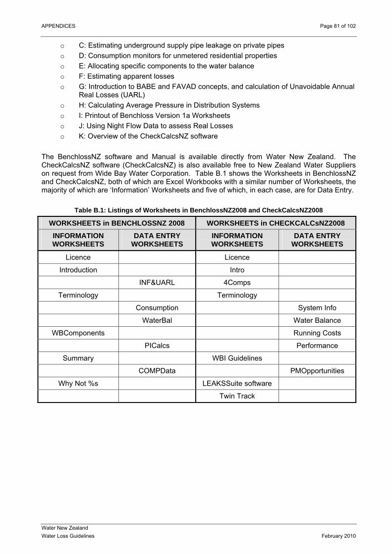
APPENDICES Page 81 of 102
o C: Estimating underground supply pipe leakage on private pipes D: Consumption monitors for unmetered residential properties o
o G: Introduction to BABE and FAVAD concepts, and calculation of Unavoidable Annual
o o Flow Data to assess Real Losses
The B chCheckCalc w Zealand Water Suppliers on re st and CheckC ich are Excel Workbooks with a similar number of Worksheets, the major of
T
o E: Allocating specific components to the water balance o F: Estimating apparent losses
Real Losses (UARL) o H: Calculating Average Pressure in Distribution Systems
I: Printout of Benchloss Version 1a Worksheets J: Using Night
o K: Overview of the CheckCalcsNZ software
en lossNZ software and Manual is available directly from Water New Zealand. The sNZ software (CheckCalcsNZ) is also available free to Ne
que from Wide Bay Water Corporation. Table B.1 shows the Worksheets in BenchlossNZ alcsNZ, both of wh
ity which are ‘Information’ Worksheets and five of which, in each case, are for Data Entry.
able B.1: Listings of Worksheets in BenchlossNZ2008 and CheckCalcsNZ2008
WORKSHEETS in BENCHLOSSNZ 2008 WORKSHEETS in CHECKCALCsNZ2008
INFORMATION DATA ENTRY INFORMATION DATA ENTRY WORKSHEETS WORKSHEETS WORKSHEETS WORKSHEETS
Licence Licence
Introduction Intro
INF&UARL 4Comps
Terminology Terminology
Consumption System Info
WaterBal Water Balance
W om sts BC ponents Running Co
PICalcs Performance
Summary WBI Guidelines
COMPData PMOpportunities
Wh ot %s LEAKSy N Suite software
Twin Track
Water New Zealand Water Loss Guidelines February 2010
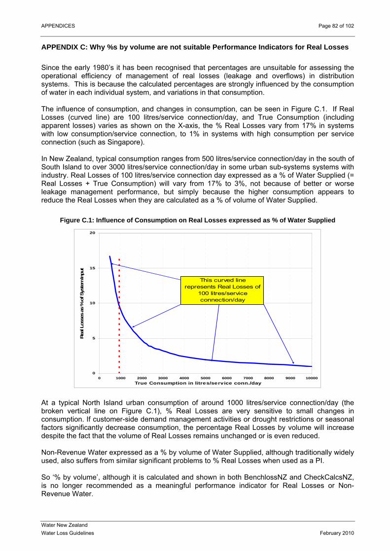
APPENDICES Page 82 of 102
APPE IX rs for Real Losses Since the e e unsuitable for assessing the opera nal f real losses (leakage and overflows) in distribution systems. Tof wa in The influen seen in Figure C.1. If Real Losse (cu y, and True Consumption (including appar t lo m 17% in systems with l co tems with high consumption per service onne ion (such as Singapore).
duce the Real Losses when they are calculated as a % of volume of Water Supplied.
Real
ND C: Why %s by volume are not suitable Performance Indicato
arly 1980’s it has been recognised that percentages artio efficiency of management o
his is because the calculated percentages are strongly influenced by the consumption ter each individual system, and variations in that consumption.
ce of consumption, and changes in consumption, can bes rved line) are 100 litres/service connection/daen sses) varies as shown on the X-axis, the % Real Losses vary froow nsumption/service connection, to 1% in sysctc
In New Zealand, typical consumption ranges from 500 litres/service connection/day in the south of South Island to over 3000 litres/service connection/day in some urban sub-systems systems with industry. Real Losses of 100 litres/service connection day expressed as a % of Water Supplied (= Real Losses + True Consumption) will vary from 17% to 3%, not because of better or worse leakage management performance, but simply because the higher consumption appears to re
Figure C.1: Influence of Consumption on Losses expressed as % of Water Supplied
0
5
10
15
put
20
0 1000 2000 00 4000 9000 1000True Consumption in lit
30 5000 6000 7000 8000res/service conn./day
0
Rea
l Los
ses
as %
of S
yste
m In This cu
represents R 100 litconnec
rved line eal Losses of
res/servicetion/day
t a typical North Island urban consumption of around 1000 litres/service connection/day (the roken vertical line on Figure C.1), % Real Losses are very sensitive to small changes in
consumption. If customer-side demand management activities or drought restrictions or seasonal factors significantly decrease consumption, the percentage Real Losses by volume will increase despite the fact that the volume of Real Losses remains unchanged or is even reduced. Non-Revenue Water expressed as a % by volume of Water Supplied, although traditionally widely used, also suffers from similar significant problems to % Real Losses when used as a PI. So ‘% by volume’, although it is calculated and shown in both BenchlossNZ and CheckCalcsNZ, is no longer recommended as a meaningful performance indicator for Real Losses or Non-Revenue Water.
Ab
Water New Zealand Water Loss Guidelines February 2010

APPENDICES Page 83 of 102
APPENDIX D: Explaining reductions in bursts following pressure management. Source: IWA Water Loss Task Force Pressure Management Group, paper by Thornton & Lambert, 2007 (Ref. 17) The conceptual approach currently being used by the Pressure Management Team of the WLTF,
attempting to develop an improved practical understanding of pressure/break frequency
operates with a substantial factor of safety, and failure rates are
inrelationships, is shown in the following series of figures.
In Figure D.1, the X-axis represents system pressure and the Y-axis represents failure rates. When a new system is created, mains and services are normally designed to withstand maximum pressures far greater than the range of daily and seasonal operating pressures for a system upplied by gravity. The system s
low. Even if there are pressure transients in the system (Figure D.2), the maximum pressures do not exceed the pressure at which increased failure rates would occur.
Figure D.1: New system supplied by gravity operates well within design maximum pressure
FAILURERATE
PRESSURE
NEW PIPES, GRAVITY SYSTEM
Figure D.2: New system with surges also operates well within design maximum pressure
o system), at some point in time the maximum operating pressure in the pipes ill interact with the adverse factors, and break frequencies will start to increase. This effect can
As the years pass, adverse factors based on age (including corrosion) gradually reduce the pressure at which the pipes will fail (Figure D.3). Then, depending upon local factors such as traffic loading, ground movement and low temperatures (which will vary from country to country,
nd from system taw
FAILURERATE
PRESSURE
NEW PIPES, SYSTEM WITH SURGES
Water New Zealand Water Loss Guidelines February 2010

APPENDICES Page 84 of 102
be expected to occur earlier in systems with pressure transients or re pumping, thangravity.
in systems
If the system is subject to surges or large variations in pressure due to changing head loss conditions, then introduction of surge control or flow or remote node pressure modulation may be expected to show a rapid significant reduction in the new break frequency. The average pressure in the system is unchanged, but the reduction of surges and large variations means that maximum pressures do not interact to the same extent with the adverse factors. If there is excess pressure in the system at the critical point, over and above the minimum standard of service for customers, then permanent reduction of the pressure by installation of pressure management (PRV, sub-division of large Zones, etc) will move the range of operating pressures even further away from the pressure at which combinations of adverse factors would cause increased frequency of failure. Figure D.4 shows the effect of reducing surges and variations in pressure and then reducing excess pressure.
Fig n
supplied by
Figure D.3: Combination of adverse factors (including surges) cause increased failure rates
COMBINATION OF FACTORS
CAUSES INCREASED
FAILURE RATE
FAILURERATE
AGE
+ C
OR
RO
SIO
N
AGE
+ C
OR
RO
SIO
N
AGE
+ C
OR
RO
SIO
N
PRESSURE
TRAF
FIC
LO
ADIN
G
TRAF
FIC
LO
ADIN
G
TRAF
FIC
LO
ADIN
G
GR
OU
ND
MO
VEM
ENT
GR
OU
ND
MO
VEM
ENT
GR
OU
ND
MO
VEM
ENT
LOW
TEM
PER
ATU
RES
LOW
TEM
PER
ATU
RES
LOW
TEM
PER
ATU
R
ure D.4: Reduction of surges and variations and reducing excess pressure limits interactiowith adverse factors and increases factor of safety
ES
FAILURERATE
AGE
+ C
OR
RO
SIO
N
AGE
+ C
OR
RO
SIO
N
TRAF
FIC
LO
ADIN
G
GR
OU
ND
MO
VEM
ENT
GR
OU
ND
MO
VEM
ENT
LOW
TEM
PER
ATU
RES
LOW
TEM
PER
ATU
RES
REDUCE PRESSURE VARIATIONSAND THEN EXCESS PRESSURE
PRESSURE
Water New Zealand Water Loss Guidelines February 2010

APPENDICES Page 85 of 102
A hypothesis as to why mains and/or service connections in some systems show large % reductions in new break frequency with pressure management, but in others the % reduction is only
•• If, before pressure management, there is already a relatively high break frequency (Red
•• (Blue Point)
of safety
Figure D.5: % reductions in break frequency influenced by initial break frequency
small, can be proposed using this concept.
Point in Figure D.5), then a relatively small % reduction in pressure may cause a large %reduction in new break frequency (towards Blue Point ). But if there is already a relatively low break frequency before pressure management Point in Figure D.5), then any % reduction in pressure (from Blue Point to Greenshould have little effect on new break frequency, but will create a greater factor and extend the working life of the infrastructure.
FAILURERATE
PRESSURE
Water New Zealand Water Loss Guidelines February 2010
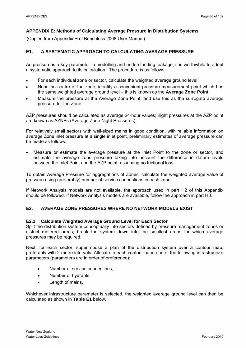
APPENDICES Page 86 of 102
APPENDIX E: Methods of Calculating Average Pressure in Distribution Systems (Copied from Appendix H of Benchloss 2008 User Manual)
E1.
a sys •• eighted average ground level; •• Near the centre of the zone, identify
the sa•• Measure the pressure at the Average Zone Point, and use this as the surrogate average
pressure for the Zone. AZP pressures should be calculated as average 24-hour values; night pressures at the AZP point are known as AZNPs (Average Zone Night Pressures). For relatively small sectors with well-sized mains in good condition, with reliable information on average Zone inlet pressure at a single inlet point, preliminary estimates of average pressure can be made as follows: • Measure or estimate the average pressure at the Inlet Point to the zone or sector, and
estimate the average zone pressure taking into account the difference in datum levels between the Inlet Point and the AZP point, assuming no frictional loss.
To obtain Average Pressure for aggregations of Zones, calculate the weighted average value of
ressure using (preferably) number of service connections in each zone.
Network Analysis models are not available, the approach used in part H2 of this Appendix should be followed. If Network Analysis models are available, follow the approach in part H3.
E2. AVERAGE ZONE PRESSURES WHERE NO NETWORK MODELS EXIST E2.1 Calculate Weighted Average Ground Level for Each Sector Split the distribution system conceptually into sectors defined by pressure management zones or district metered areas; break the system down into the smallest areas for which average pressures may be required. Next, for each sector, superimpose a plan of the distribution system over a contour map, preferably with 2-metre intervals. Allocate to each contour band one of the following infrastructure parameters (parameters are in order of preference):
• Number of service connections; • Number of hydrants; • Length of mains.
Whichever infrastructure parameter is selected, the weighted average ground level can then be calculated as shown in Table E1 below.
A SYSTEMATIC APPROACH TO CALCULATING AVERAGE PRESSURE
As pressure is a key parameter in modelling and understanding leakage, it is worthwhile to adopt tematic approach to its calculation. The procedure is as follows:
For each individual zone or sector, calculate the w a convenient pressure measurement point which has
me weighted average ground level – this is known as the Average Zone Point;
p If
Water New Zealand Water Loss Guidelines February 2010
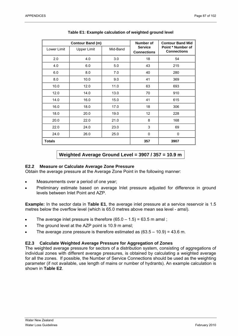
APPENDICES Page 87 of 102
Table E1: Example calculation of weighted ground level
Contour Band (m)
Lower Limit Upper Limit Mid-Band Service Connections
Point * Number oConnections
Number of Contour Band Mid f
2.0 4.0 3.0 18 54
4.0 6.0 5.0 43 215
6.0 8.0 7.0 40 280
8.0 10.0 9.0 41 369
10.0 12.0 11.0 63 693
12.0 14.0 13.0 70 910
14.0 16.0 15.0 41 615
16.0 18.0 17.0 18 306
18.0 20.0 19.0 12 228
20.0 22.0 21.0 8 168
22.0 24.0 23.0 3 69
24.0 26.0 25.0 0 0
Totals 357 3907
Weighted Average Ground Level = 3907 / 357 = 10.9 m
E2.2 Measure or Calculate Average Zone Pressure Obtain the average pressure at the Average Zone Point in the following manner: •• Measurements over a period of one year; ••
servoir is 1.5 etres below the overflow level (which is 65.0 metres above mean sea level - amsl).
Preliminary estimate based on average Inlet pressure adjusted for difference in ground levels between Inlet Point and AZP.
Example: In the sector data in Table E1, the average inlet pressure at a service rem •• The average inlet pressure is therefore (65.0 – 1.5) = 63.5 m amsl ; •• The ground level at the AZP point is 10.9 m amsl; •• sure is therefore estimated as (63.5 – 10.9) = 43.6 m.
obtained by calculating a weighted average e z Service Connections should be used as the weighting
param er ins or number of hydrants). An example calculation is shown in T
The average zone pres E2.3 Calculate Weighted Average Pressure for Aggregation of Zones The weighted average pressure for sectors of a distribution system, consisting of aggregations of
dividual zones with different average pressures, isinfor all th ones. If possible, the Number of
et (if not available, use length of maable E2.
Water New Zealand Water Loss Guidelines February 2010

APPENDICES Page 88 of 102
Table E2: Example calculation of weighted ground level
Area
Reference vice
ions Avera
Presice ZP
Number of SerConnect
ge Zone sure
Number of servConnections * A
A 420 55.5 23 310 B 527 59.1 146 31 C 443 69.1 611 30 D 1352 73.3 102 99 E 225 64.1 423 14 F 837 42.0 154 35 G 1109 63.7 643 70 H 499 56.3 094 28I 1520 57.0 640 86
6932 122 419
Weighted average pressure for the hole area = 419,122/6932 = 60.5 metres w
3. AVERAGE ZONE PRESSURES USING NETWORK MODELS
Calculateus mally have a number of properties, a
late the weighted
s w ted average ground level, and an AZP point are
E
E3.1 B
Weighted Average Ground Level for Each Sector eca e each node of a Network Analysis Model will nor
datum ground level, and an average pressure value, it is relatively easy to calcuaverage pressure for all the nodes in the model (or any defined part of it). It i orthwhile, however, to ensure that a weighdefined for each zone/sector, as these will occasionally be required for test measurement.
Water New Zealand Water Loss Guidelines February 2010

APPENDICES Page 89 of 102
APPENDIX F: Meter La
F1: WHA MET EY In Water Balance calculation, the etered volume ater Supplied' sh ompared to the actual consumption volume o 12-month 'Wa ar' which, in New Zealand, normally runs from 1st July to 30th June inclusive. In New Zealan eter reading cies for residen operties seem to ally every 6 or 12 months, every 3 month on-residential ies or large user ge systems, Water Suppliers tend to operate a rolling reading cycle. In medium and small systems, or those with several smaller Water Supply Systems, the meter reading cycle for ea ual system may be compl in a few wee th smart meteri data collection, the meter reading cycle be completed ew days, althou ere will usually re me reading and billing queries to be resolved. The effect of failure to make a r lag’ a n be simply demonstrated from the
llowing ustralian example. The first meter reading cycle commences on the 1st ater Year (1st July), takes 3 months to complete, and there are 4 meter reading cycles per year.
raph 1 shows quarterly data (in Ml/d) for Water Supplied and Recorded Metered Consumption
duction due to ted, in some quarters the
etered consumption recorded in the quarter equals or even exceeds volume of water entering e between the two lines)
g Calculations: Methods and Examples
T ARE ER LAG ADJUSTMENTS; WHY ARE TH NEEDED?
bulk m of 'W ould be cver a ter Ye
d, m frequen tial pr be typicand s for n propert s. In lar
ch individeted ks. Wi ng and automatic can in a f gh th main so
‘mete djustment cafoW
A day of a new
Gover the period 2005 to 2009, with some seasonal variation and a general reimposition of drought restrictions. If no meter lag calculation is attempmthe system in that quarter. So the Non-Revenue Water (the differencappears to be highly variable from one meter reading cycle to the next, and in some quarters has a zero or even negative value Graph 1: Comparison of Quarterly Water Supplied and
Recorded Consumption in Meter Reading Cycles for same Quarter, July 2005 to June 2008
-10.020.030.0
40.050.060.0
Q105/06
Q205/06
Q305/06
Q405/06
Q106/07
Q206/07
Q306/07
Q406/07
Q107/08
Q207/08
Q307/08
Q407/08
Q108/09
Ml/d
ay
Water Supplied Recorded Consumption
Water New Zealand Water Loss Guidelines February 2010
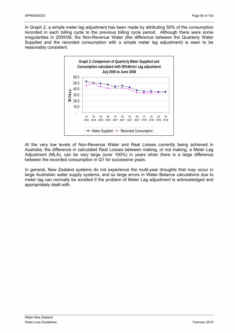
APPENDICES Page 90 of 102
In Graph 2, a simple meter lag adjustment has been made by attribg cycle to the previous billing cycle period.
uting 50% of the consumption Although there were some
regularities in 2005/06, the Non-Revenue Water (the difference between the Quarterly Water is seen to be
general, New Zealand systems do not experience the multi-year droughts that may occur in rge Australian water supply systems, and so large errors in Water Balance calculations due to eter lag ent is acknowledged and ppropriately dealt with.
recorded in each billinirSupplied and the recorded consumption with a simple meter lag adjustment)
nt. reasonably consiste
At the very low levels of Non-Revenue Water and Real Losses currently being achieved in Australia, the difference in calculated Real Losses between making, or not making, a Meter Lag Adjustment (MLA), can be very large (over 100%) in years when there is a large difference between the recorded consumption in Q1 for successive years.
Graph 2: Comparison of Quarterly Water Supplied and Consumption calculated with 50% Meter Lag adjustment
July 2005 to June 2008
10.020.030.040.050.060.0
Ml/d
ay
-Q1
05/06Q2
05/06Q3
05/06Q4
05/06Q1
06/07Q2
06/07Q3
06/07Q4
06/07Q1
07/08Q2
07/08Q3
07/08Q4
07/08
Water Supplied Recorded Consumption
Inlam can normally be avoided if the problem of Meter Lag adjustma
Water New Zealand Water Loss Guidelines February 2010

APPENDICES Page 91 of 102
APPENDIX G: Additional Information on Bulk Metering There are many different types of bulk meter - Electro-magnetic, Ultrasonic, Venturi, Dall tube, Orifice plate, Insertion meters, Helix meters, Vortex shedding, Turbine, Propeller etc. All bulk
eters are sensitive to distortion of the velocity profile in the mains, to a greater or lesser extent, which is wh upstream and downstream of the ld not be compromised. Sensitivity to velocity profile dist •• Very High, fo•• High, for ultr•• Medium/Low Each of these meter t these (from Ref 19
rs
my manufacturers’ recommendations on minimum lengths of straight pipe
meter (expressed as a number of pipe diameters) shouortion is generally:
r insertion meters asonic and helix meters , for electromagnetic meters
ypes has its own particular advantages and disadvantages. Some of) are shown in the Table below.
Advantages and Disadvantages of different types of Bulk Mete
Type of Bulk Meter Advantages Disadvantages High accuracy, linear response High sensitivity to flow distortion Great reliability. No mobile Need for electric supply parts subject to wear Small head loss
ltrasonic (transit time) U
Moderate cost Not suitable for billing (this may change with new standards)
High accuracy, linear response Need for electric supply Great reliability. No mobile parts subject to wear
Needs protection against electrical storms; subject to failure from lightning strikes
Small head loss, low operation cost
Not suitable for billing (this may change with new standards)
Electromagnetic
Medium/low sensitivity to flow profile distortion
Low cost, especially for large diameters
Low measurement reliability compared to other technologies
A single insertion probe can be used at different locations
Very sensitive to distortion of velocity profile
Can be used in water with suspended solids
Need to drill a hole in the pipe
Insertion
Small head loss Narrow range of measurement Usable in difficult working conditions
Error curve is sensitive to velocity profile quality.
Wide measuring range Use of tranquilising lengths of pipe upstream of meter may be necessary
Metering module can be replaced in existing casing
Low sensitivity for low flow rates
Can be installed in virtually any position
Horizontal Helix Meters
Pulse emitters can be attached to flow totalisers
Impact of large suspended solids may damage the metering module; the use of stone strainers is recommended
Regular calibration of electronics is normal practice, but this should not be assumed to imply that the meter is recording the correct flows. The meter may be incorrectly sized or of an inappropriate type for the flow profile at the particular location, and facilities for independent flow validation are rarely provided - so regular flow validation is not normally practised. During droughts, bulk meter flows which are much lower than original design flows, or reversal of flows, may occur, leading to under-registration of actual flows.
Water New Zealand Water Loss Guidelines February 2010

APPENDICES Page 92 of 102
Other factors affecting bulk meter data accuracy (Ref. 20) in
clude:
•• Changes to Meter Geometry: caused by Corrosion and Corrosion products, other deposits and debris, and mechanical wear.
•• Installation problems pipework configuration upstream or downstream of the meter, mis-alignment, and meters not running full.
•• Signal Processing Errors, which can be caused by Span Errors (when setting up or checking the meter) and other calibration factors.
SCADA systems involve manipulation of data •• during transmission and possible data loss perating
part of Water Balance
when SCADA systems are not o Validation of bulk metered volumes is therefore an essentialcalculations. Bulk Meter Validation Options (Ref. 20) include: •• Volumetric tests, involving drawing down an upstream tank or clear well, or filling a
downstreamust be large test accuracy required - what is the or a
o the measured ial measurement wat quipment
o the tank must b ing isolated foraccuracy requi
o a static test muo for accurate me imensions evel
or or high •• Mass Balances
tank, are a good practical option, if possible. o the tank m
resolution f enough to provide the
1mm difference in level? level drop needs to substantiaer level measuring e
lly exceed the potenterror of the
e capable of be a sufficiently long period to provide the red st be conducted on the tank to casurement of tank d
heck for leakage / valves passing and water depth, use an ultrasonic l
sens accuracy pressure transducer are nd treatment works
(raw water, process wo temporary meteo if inconsistenci d in the mass balanc tion is necessary.
mass balances meters in serie r between groups of bulk
•• Test Meters in Series
a useful first step, for multiple ater meters, output meters etc
sets of meters arou)
rs may be needed on any pipees are foun
s not normally metered e, further investiga
o can also be used to check for inconsistencies between two bulk s, where water is exported fro
meters, for example on transmism one system to another; osion mains
: Insertion meters o do not locate ino above DN600, s to try too above DN1200, distances should be further in or a
f twoo always determio always underta e
•• Test Meters in Series
sertion meters within 50 pipe diameters of pumps, fittings or bends double these distance offset possible swirl problems
creased; use 2 plane data probes minimum o pairs of ultrasonic meters
ne the velocity profile, experience shows that itke the test with the insertion m
is rarely uniform ter at the pipe centreline
: Clamp-on Ultrasonic meters nces from pumo Minimum dista ps, fittings or ends as for Insertion Meters; use a b
minimum of two pairs of ultrasonic meters above DN1200 o always measure pipewall thickness using ultrasonic tool, and always use silicon
grease to ensure good contact •• Portable Test Rigs may be used for checking small bulk meters
Water New Zealand Water Loss Guidelines February 2010

APPENDICES Page 93 of 102
Common Issues in Validating Bulk Meters (Ref. 20) include: •• Data Chain Analysis: test across the normal operating range of the meter, using 3 flow rates
if operationally possible o record local (and remote) integrator readings at start and end of each test o log meter output (4-20mA / pulse) from primary sensor o obtain data for period of test from SCADA and compare with on-site readings to check
if SCADA has introduced additional errors •• Conclusions of Bulk Meter Validation Test: calculate the error range of the validation
method; if recorded bulk meter flows during the test are: o within this error range, the bulk meter is deemed to be OK.
rded volumes, take appropriate action.
bulk meters include:
.7% higher than on-site readings o
corrected, one under-reading by 3.3%, the other by 4.8%, based on volumetric tests. o
2 %, o
meter but billing system configured to calculate forward flows only o s. Some bas ef. 20) include:
o er's specifications and accuracy data
o or
o once
hly) mass balances where possible, to identify
o -passes
o s ppl
o ns (or
ed/installed/maintained, should not be
o if mo of their total volume should
o outside this error range, assume the bulk meter has a systematic error, correct recent reco
ome examples of Errors found when validatingS
o main meter from treatment works over-sized for drought flows; mass balance and volumetric
test indicate under-reading of 1% to 4%. SCADA volumes 1two ultrasonic meters at a treatment works: one using incorrect configuration file; when
Buried meter recording flows when no flows passing through it; over-reading by 16% to suspected due to water ingress. 0
Open by-pass at one export point; bi-directional flows at another, correctly recorded by
An unmetered import point had been opened in an emergency, but not closed afterward
ic actions to reduce Bulk Metering Errors (R
find, and retain in an accessible location, manufacturfor all bulk meters record if bulk meters are not installed in accordance with manufacturers instructions (current best practice), with photographs provide on-site validation facilities to facilitate volumetric checking of bulk meters at least
per year o carry out regular (approximately mont
changes and inconsistencies identify and limit locations where bi-directional flows may occur, or bulk meter bymay be left open. ensure that all bulk meters have a cumulative register on-site, with an emergency power
y in case of temporary loss of power ualways use the bulk meter cumulative register readings for water balance calculatioensure SCADA data correspond with them)
o the accuracy of 1 bulk meter, correctly selected/sizassumed to be better than +/- 2%.
re than one bulk meter supplies a system, the random errordecrease with the number of meters.
Water New Zealand Water Loss Guidelines February 2010

APPENDICES Page 94 of 102
APPENDIX H: Typical Installation of a Water Meter and Pressure Reducing Valve
Water New Zealand Water Loss Guidelines February 2010

APPENDICES Page 95 of 102
APPENDIX I: Pressure Management in Waitakere City – A Case Study
Zoran Pilipovic, Richard Taylor, EcoWater, Waitakere City Council, New Zealand
[email protected], [email protected]
APRIL 2002 ABSTRACT
1996, as part of Council’s Water Cycle Strategy, a pressure standardisation rogramme to permanently lower the average supply pressure citywide was implemented ith the aim of reducing water loss and water use. The experience gained during the 994/95 Auckland water shortage had confirmed that there was considerable scope to duce pressures in many areas.
ince 1996 water pressures have been reduced in over 60% of the reticulated area of the ity, with the average pressure reduced from 710kPa to 540kPa. As a result of this rogramme water loss from the network has been reduced, there has been a reduction in e frequency of mains breaks and it is likely that the life of water pipeline assets has een extended. Furthermore both pressure and demand management initiatives have duced per capita water use in the city by more than 10%.
network computer model was used as a design tool to check the network under various ressure regimes and cost benefit analyses were carried out for various design scenarios. ire sprinkler systems were checked as part of the design process. Minimum service tandards were not reduced and in some cases pressures were actually increased. This aper covers the various aspects of the design, the implementation and the results of the ressure standardisation programme.
EY WORDS
ressure management, leakage, demand management, pressure reducing valve RV), modelling
troduction
aitakere City Council’s water business unit (EcoWater Solutions) purchases water from uckland’s bulk supplier (Watercare Services Ltd) to supply residents and businesses in e city. Bulk water is metered at 28 bulk supply points. All consumption is metered with
urrently around 59,000 connections made up of residential (79%), industrial/commercial 5%) and agricultural (6%) users. The network comprises 1267km of water mains nging in size from 50mm to 375mm. Approximately 60% of the mains are asbestos
ement, 30% PVC and the balance are polyethylene, steel, galvanised and cast iron.
late 1995 Waitakere City Council combined its “Eco city” philosophy with the lessons arnt during the 1994/95 Auckland water shortage to develop a Water Cycle Strategy at promoted sustainable water management solutions at a local level. During the water
hortage pressures were reduced as an emergency measure. In 1996, as part of the ater Cycle Strategy, it was decided to implement a programme to permanently lower
the average supply pressure citywide to reduce water loss and water use. The water
Inpw1re Scpthbre ApFspp K P(P In
WAthc(1rac InlethsW
Water New Zealand Water Loss Guidelines February 2010
APPENDICES Page 96 of 102
shortage had confirmed that there was considerable scope to reduce pressures in many areas as existing pressures were often well in excess of 300kPa. S area of sures were altered for 35,000 consumers, and in most cases pressures were reduced by between 150 and 500kPa. Pressure fluctuations were also reduced in many
sult of the programme. Water loss from the network and the frequency of mains breaks tly reduced as a result of the programme and it is also likely that the life of
ater pipeline assets has been extended. With advanced pressure management
affected systems dealt with dividually. This paper covers the various aspects of design and implementation of the
unstable pressure in the water supply system on etwork assets has been recognized in many countries since the early 1980's. The
likened to high and fluctuating blood pressure in the human body. Since 980 a number of research activities at a national level have been carried out, for
razil, and Malaysia (Ref 2). Awareness of pressure management and s effects on network assets is now much more acknowledged then previously and a new
discipline, pressure management, has developed. In many water ssure management is widely accepted as having benefits in:
ince 1996 water pressures have been reduced in approximately 60% of the reticulatedthe city with the average pressure reduced from 710kPa to 540kPa. Pres
areas as a rehave significanwtechniques, future upgrading works may also be deferred as pressures can be increased only during periods of high demand. As a greater number of smaller sub zones can now be managed and monitored, leak detection activities are more focussed. Pressure and demand management initiatives have reduced per capita water use in the city by more than 10%. Design work and implementation was carried out in house by water engineering staff. A network model was used as a design tool to check the network under various pressure regimes, and cost benefit analyses were carried out for the different scenarios. Minimum service standards were not reduced. In some cases zone boundaries were altered and in a few small areas pressures were increased to improve service. The impact of reduced pressures on fire sprinkler systems was considered and inpressure standardisation programme, and the main results. Background The detrimental effect of excessive andnproblem can be1example, in the UK (Ref 1), and pressure management case studies have been analysed in the UK, Japan, Bitwater supply authorities, pre
• Demand Management - Less consumption from pressure related uses of water;
• System Deterioration - Extended useful life of infrastructure; • Water Losses - Reduced leakage and fewer new leaks; • Maintenance costs - Reduced frequency of main breaks; • Customer service - Better service due to less water supply interruptions.
The UK Water Research Centre and Japan both developed average relationships between leak flow rate and system pressure around 1980. The FAVAD concept, developed in 1994 by John May in the UK, has proved to be the most reliable approach, and further work carried out since 1994 by the IWA Water Loss Task Force has confirmed the N1 exponent in the FAVAD relationship is dependent on the type of pipeline materials; Figure 1 below (refer Ref 2) shows a range of pressure/leakage relationships relating to
Water New Zealand Water Loss Guidelines February 2010

APPENDICES Page 97 of 102
various N1 values. There is now a good understanding of the way networks respond to pressure changes. Our experience has proven that an N1 value of 1.5, which relates to igh pressure systems with predominantly non-metallic pipe materials without significant
NVESTIGATIONS
DESIGN CRITERIA DELIV Y S The aim of the programme was to reduce the main tow measured at the meter. For design purpose
hleakage, applies particularly well to the reticulation in Waitakere City.
0 . 6 0
0 . 8 0
1 . 0 0
1 . 2 0
1 . 4 0
f Lea
kag
e R
ates
L1/
Lo
N 1 = 0 . 5 0
N 1 = 1 . 0 0
N 1 = 1 . 1 5
N 1 = 1 . 5 0
0 . 0 0
0 . 2 0
0 . 0 0 0 . 1 0 0 . 2 0 0 . 3 0 0 . 4 0 0 . 5 0 0 . 6 0 0 . 7
R a t io o f P r e s s u r e
Rat
io
0 . 4 0 o
N 1 = 2 . 5 0
Figure 1: Relationship between Sys
PILOT ZONE I The first stage of the programme was designed aappeared to be no previous experience in comprin New Zealand. Massey East Zone, with 1,detailed network investigations. The area was sIn the lower zone the pressure was reduced by 5were reduced 200kPa. The results from the piOver the period, the average minimum night flowfrom 1.2 l/s to 0.6 l/s and the total water demcustomers complained about low pressure, apressure and showers. A plumber at Council’s co
ER TANDARDS
avetain he current minimum service standard
flunder peak demand and 100kPa for background It was also necessary for compliant fire sprinkler compliant after the pressure adjustments. This wlegal requirement. A calibrated network modelmanagement options and to check that the supply
Water New Zealand Water Loss Guidelines
N 1 = 1.5 Applicable for Waitakere City
roblems.
inute s 300kPa residual pressure was required
0 0 . 8 0 0 . 9 0 1 . 0 0 1 . 1 0 1 . 2 0
s P 1 /P o
tem Pressure and Leakage
s a trial exercise in a pilot area, as there ehensive pressure management projects 250 connections, was selected for the plit into a lower and an upper sub-zone. 00kPa while in the upper zone pressures lot investigation confirmed expectations. , as an indicator of losses, was reduced and reduced by up to 14%. Only five ll relating to problems with hot water st quickly remedied these p
rage supply pressure across the city but of 250kPa pressure and 25 litres/m
use plus fire flows.
systems installed prior to 1996 to remain as a responsible approach rather than a was used to analyse various pressure to critical points was not compromised.
February 2010

APPENDICES Page 98 of 102
SELECTION AND DEVELOPMENT OF PRESSURE ZONE AREAS The main urban areas of Waitakere City and the northern part of the city i.e. Henderson,
latively low lying and border onto the upper reaches of the Waitemata Harbour. These reas were typically supplied directly via the Watercare trunk water mains with a static
pressure of 115m (HGL) and daily pressure fluctuations between 95 and 115m(HGL). hus improvem ts could be achieved by implementing pressure management, firstly by e permanent rezoning of existing areas where the HGL could be reduced from 115m to
5m or 75m, and secondly, by optimising pressure regimes. As a first step pressure ducing valves with basic fixed outlet pressure characteristics were installed, as the ater supply zones were comparatively small. The use of time variable and flow ompensating valves was seen as an enhanced option for a future development.
n overview of the system r four supply zones / sub – ones is given in Table 1.
YDRAULIC SURVEY AND MODELLING
hydraulic survey using solid-state pressure loggers to monitor performance was cognized as an ctions. Initially
ressure loggers were used to calibrate the network model and to record the pressures of the pressure standardization programme. Prior to d during the implementation phase of the programme,
02 odes and 2,909 pipes with a combined length of 668.1 km. Demand is modelled by
ock (a nodal polygon) as the unit of demand modelling. All elements ing pumps, supply points, reservoirs, and pressure control valves
actual operating conditions.
Hobsonvre
ille, Whenuapai, Lincoln, Swanson, Te Atatu, Kelston, New Lynn, Glen Eden, are
a
T enth6rewc A rezoning pressure reduction foz
H Are essential step prior to the introduction of pressure redupoccurring prior to implementation
aking changes to the network, anmpressure loggers were used to closely monitor the changes and to verify pressures at the supply points, the furthest points in the zone and the highest points (the critical points), as well as for analysis of PRV performance. A dynamic hydraulic model (WesNet / InfoWorks WS) was used for analysing how the network would respond to a change in pressure regime, for designing the pressure standardization programme and for operational and planning needs. Separate models were developed and calibrated for each distribution zone but the intention is to combine these into a global model as a further enhancement to the modelling. To create the model geometry for each zone GIS graphical files in CGM form were imported and nodes nd pipes traced directly over background GIS maps. In total the models have 2,5a
ndefining a demand bl
f the network includowere modelled to match The models are very stable and the “goodness of fit” between the computed and measured results is generally in the order of 5 %. Models for the entire Waitakere City water supply system were completed 'in house' over a period of 9 months.
Water New Zealand Water Loss Guidelines February 2010

APPENDICES Page 99 of 102
Table 1: Summary of Pressure Reduction in Water Supply for Zones 4, 5, 6 and 15.
ZONE Initial Reduced Pressure Reduced Number of s
No. SUPPLY
and Sub Zone Maximum Pressure
Max. Pressure
Reduction Daily Pres. Fluctuations
Connection
m M m m 4 LINCOLN – SWANSON 7.300 Lincoln-Swanson Central Sub Zone 115 75 40 20 4,900 Massey Reservoir Sub Zone 115 100 15 20 1,900 Simpson Rd Sub Zone 115 100 15 25 500
5 TE ATATU – KELSTON – GLENDENE 7,000 Te Atatu Peninsula Sub Zone 100 65 35 25 3,100 Te Atatu South 100 75 25 20 3,000 Kelston Sub Zone 100 65 35 10 900
6 HENDERSON 5,800 Henderson Central Sub Zone 115 75 40 20 4,700 View Rd Sub Zone 115 95 20 20 900 Pine Ave. Sub Zone 115 90 25 25 200
15 WEST HARBOUR 3,000 115 95 20 15 1,700
West Harbour Upper Sub Zone West Harbour Lower Sub Zone 115 65 50 15 1,300
PROGRAMME IMPLEMENTATION EQUIPMENT SELECTION AND INSTALLATION The results of the hydraulic survey and network modelling were used in selecting and sizing pressure-reducing valves, water meters etc for each site. The standard installation onsisted of a strainer and PRV installed in one chamber, and the water meter installed in
n of the programme was carried out moothly without any significant operational difficulties. Furthermore there have been no
00 properties) as carried out with only 1% of affected customers contacting council with a pressure lated complaint. Half of these complaints were attributable to customer’s internal
lumbing problems such as hot water cylinders and showers. A plumber quickly resolved these problems (often only adjustment) at council’s expense. Some problems took longer to resolve. Problems with plumbing systems and inadequately sized pipes or highly encrusted private galvanized pipes became evident at lower pressures. In some cases
ca separate downstream chamber. The pressure standardisation programme involved bringing back into service 15 existing PRV’s at bulk supply points and the installation of 22 new PRV’s. METHODOLOGY Once the pressure reducing valves were installed, the pressure reduction exercise was usually carried out in two steps. Firstly, pressure was reduced half way to the target level and a few days later the pressure was adjusted to the final level. Over this period, data loggers recorded inlet and outlet pressures at the PRVs and pressure at critical points in the zone. In the majority of cases the implementatiossignificant reticulation problems during subsequent summers when temperatures have been high and demand at record levels. The implementation of the entire pressure standardisation programme (35,0wrep
Water New Zealand Water Loss Guidelines February 2010

APPENDICES Page 100 of 102
the pipe for a new private line was supplied free. Council staff rectified any service connect
lems in th system we c y Vcyclic pressure , unstable p i iv a rduring peak demand and valves performing as a rect ratio valve rather than as a pressure-reducing valve. In one or two cases the PRV failed and there was a sudden return to original pressures, which had a very undes able effe t on the n twork. p b ulty es, one -hand ve, and inary vb n rned on af ainten . C ER EMS An important aspect of the programme was dea with tomer tions. p g re standardisation progra e’ whpressures were being standardised across the city. Notification of the pro mme speedy response to any c arising from changes operap s l. A letter with info ion ab lanne ctivities a pres hure were delivered to all affected cust mers. E ry cuscomplaint was followed up promptly and i tigated taking tests a e metehou opriate action was taken to e problem
o ensure fire sprinkler systems remained compliant after the pressure changes were ngaged to access the impact of reduced pressures
n 70 fire sprinkler systems within the city. Where a problem was envisaged for a used to confirm final pressures at the location
nd then the designer of the system was engaged by Council to identify the most cost
he capital cost for the programme was $850,000 spread over three financial years. This ered the cost of installing 22 new pressure control sites, laying a few new
hort pipelines, road crossings, installing new valves, fire system consultants,
ion problems (restricting flow to the meter) at Council’s cost. Prob e distribution
fluctuationsre mainly aused b
rrespect poor PRe of dem
performannd, pressu
ce, e.g., e drops ressures
di
ir c e Other ro lems encountered were due to fa valv left val ord alves ei g left off instead of being tu ter m ance
USTOMER RELATIONS AND FIRE SPRINKL SYST
ling cus relamm
The ro ramme was communicated as a ’pressu ereby
gra and a ustomer complaints in tional
re sure was essentia rmat out p d a and ssure tandardisation broc o ve tomer
nves by flow t th r, the se tap and a pressure test at the nearest hydrant. Appr
nsure there were no outstanding s. Tmade a specialist fire engineer was eoparticular system the network model wasaeffective means of overcoming the problem. Some reticulation improvements and upgrading of internal sprinkler installations were carried out and funded by Council to overcome such problems. COST BENEFIT OF THE PROGRAMME Texpenditure covsmodifications to existing fire sprinkler systems, plumbing costs and public notification. The key benefits of programme are summarised below. ••
be largely responsible for the overall per capita
Less water consumption per capita largely a result of a reduction in pressure dependent usage, e.g. showers, garden hoses etc. Per capita water consumption in Waitakere City has reduced by more than 10 % since 1992/93 due to the introduction of various demand and pressure management techniques. Pressure management however, is known to reduction (Ref 3). It has been estimated that the quantity of wastewater per capita has also reduced by approximately 4% - 5%. One percentage of wastewater volume represents a cost to Waitakere City of approximately $100,000 per year.
•• Less frequency of major breaks (i.e. major breaks on a water main or saddle) as shown in Figure 2. In 2000 / 01 the average number of breaks per month was 48 (or 10 breaks per 1,000 connections). Prior to 1996 the average number of breaks per month was more than 65 (or 15 breaks pre 1,000 connections). Less breaks means
Water New Zealand Water Loss Guidelines February 2010

APPENDICES Page 101 of 102
reduced maintenance costs and less supply interruptions and consequently improved customer service.
Figure 2: Waitakere City – Number of Major Breaks per 1,000 Connections Per Annum
••
••
hat
••
Less water losses. The non-revenue water loss reduced from 14.7 % by volume for the 12 months ending June 1996 to 10.5 % for the 12 months ending June 2001 (Figure 3). Reducing water losses by one percentage point represents an annual saving to Waitakere City of $ 65,000, i.e. the 4.2% reduction represents a total saving of $273,000 per annum.
Figure 3: Waitakere City – Water Losses, % Non revenue Water By Volume
More efficient leak detection is now possible as 14 new sub zone areas with 22 control points (meters) are now monitored, some using telemetry. This means tthe awareness time of unreported leaks is reduced with significant cost savings. The life expectancy of water network assets, where pressures have been reduced and pressure fluctuations minimised, has probably been extended by 10 to 20 years
19.520
Nu
15.614.7
12.511.5
12.912.1
10.510
15
on R
even
ue W
ater
by Vo
l
0
5
93 / 94 94 / 95 95 / 96 96 / 97 97 / 98 98 / 99 99 / 00 00 / 01
%
Pressure Standardisation
25
16.7
12.3
16.214.9
12
14.513.8
15
20
1,0
00 C
onne
ctio
ns
High num ber of breaks in sum m er 1998 - 99 due to "E l N ino" effect
.8
11.210.0
0
5
92/93 93/94 94/95 95/96 96/97 97/98 98/99 99/00 00/01
Maj
or b
reak
s pe
r
Low num ber of breaks in winter 10 1994 related to water shortage
Pressure Standardisation
me
Water New Zealand Water Loss Guidelines February 2010

APPENDICES Page 102 of 102
•• pulation growth is now possible as existing surplus
upstream pressure at control points can be used to increase the capacity of the
r other water utilities, however it is evident that the benefits of pressure management re too as utlined above are robust and will generate ongoing financial benefits.
ACK Waitamanagement and how this can be achieved at a local level. This paper outlines one of
aitakere City Council for being a progressive city and EcoWater management staff for eir strong support in the implementation of the pressure standardisation programme.
EFERENCES
U.K. Water Industry (1994) “Managing Leakage” ISBN 1 898920 06 A. Lambert, S. Meyers, S. Trow (1998) “Managing Water Leakage” ISBN 184083 Montgomery Watson NZ Ltd (1999) “Waitakere City-wide water demand model”
ONTACTS oran Pilipovic, Private Bag 93109, Henderson, Waitakere City, New Zealand, [email protected] Ph 0064 9 836 9826 Fax 0064 9 835 0293 ichard Taylor, Private Bag 93109, Henderson, Waitakere City, New Zealand [email protected] Ph 0064 9 836 9827
Less capital expenditure for future upgrading of the system. Savings in capital upgrading costs to meet po
system by simply converting the fixed pressure PRV’s to flow modulating PRV’s •• One benefit often overlooked is that private plumbing systems are subjected to a
reduced pressure, which in turn reduces faults on private water systems. A very simple but conservative overall cost benefit for the programme gave a payback period of 3.3 years. This ignores the financial benefits of deferred capital works, reduced wastewater volumes and extended life of assets etc. CONCLUSIONS For water supply authorities the continuous improvement and development of operational network management is essential to gain the greatest efficiencies in water distribution. Initial results of the pressure standardisation programme in Waitakere City have confirmed that pressure management is a significant operational technique that can be used to great advantage with many benefits. The fact that Waitakere City is supplied by a bulk supplier (Watercare Services Ltd) via 28 bulk supply points supplying 17 discrete water supply zones meant that pressure reduction was perhaps easier to accomplish than foa great to be ignored by any water supplier. The benefits of the programmeo
NOWLEDGEMENTS
kere City Council has pursued a progressive approach towards sustainable water
the achievements resulting from this strategic direction. The writers would like to thank Wth
R 1)
2)
3)
CZzRri
Water New Zealand Water Loss Guidelines February 2010
![Water Loss Quality Cantwell2013.pptx [Read-Only]ucce.ucdavis.edu/files/datastore/234-2540.pdf · About 3-4% weight loss = soft head Texture and Water loss Water Loss and Fruit Ripening](https://img.pdfslide.us/doc/110x75/5f0d1eba7e708231d438c70a/water-loss-quality-read-onlyucceucdavisedufilesdatastore234-2540pdf-about.jpg)