Water hammer in pumped sewer mains

by

Torben Larsen

Department of Civil Engineering, Aalborg University

EVA udvalget

Spildevandskomiteen

Ingeniørforeningen i Danmark

The EVA committee

The Danish Water Pollution Committee

The Danish Society of Engineers

November 2006

Preface This publication is intended for engineers seeking an introduction to the problem of water hammer in pumped pressure mains. This is a subject of increasing interest because of the development of larger and more integrated sewer systems. Consideration of water hammer is essential for structural design of pipelines.

The text is written by Torben Larsen, who is a professor of environmental hydraulics at the Department of Civil Engineering, Aalborg University. Torben Larsen has many years of experience with computer simulations of water hammer in sewer systems.

The aim of the EVA committee is to disseminate best practices within the field of urban drainage. Dissemination takes place mainly through meetings, a periodical and our web-site (www.evanet.dk). Historically we have taken much interest in modelling of sewer systems. As such the committee welcomes this publication. We hope that it will be used throughout teaching of students as well as used to solve practical engineering problems in real life.

All comments are most welcome.

Karsten Arnbjerg

Chairman of the EVA Committee, MSc, PhD

November 8, 2006

Addresses The EVA committee The Danish Water Pollution Committee The Danish Society of Engineers Kalvebod Brygge 31-33, DK-1780 København V, Denmark Torben Larsen Department of Civil Engineering, Aalborg University Sohngaardsholmsvej 57, DK-9000 Aalborg, Denmark e-mail: torben.larsen@civil.aau.dk

2

Table of contents 1 Introduction 5

2 Steady state hydraulics for pump systems 6 2.1 Pressure versus pressure head 6 2.2 Energy equation 6 2.3 Duty point 7 2.4 Pump characteristic 8 2.5 Pump cavitation 8 2.6 Pipeline characteristic 9 2.7 Self-cleansing 12 2.8 Air pockets 13

3 Water hammer and cavitation in pumped mains 14 3.1 Water hammer 14 3.2 Cavitation 14 3.3 Example of measurement of water hammer 15

4 The influence of water hammer on the design of pipelines 17 4.1 Effect of maximum and minimum internal pressure 17 4.2 Fatigue 19 4.3 Practice for pipe design 21

5 Basic principles for water hammer 22 5.1 Celerity of the pressure wave 22 5.2 Joukowsky’s equation 23 5.3 Reflection of water hammer 24 5.4 Reflection in joints between pipes in series 26

6 Water hammer in pumping mains 28 6.1 Pump start-up 28 6.2 Pump shut-down 29 6.3 Inertia of the pump 31

7 Precautions against water hammer at pump shut-down 33 7.1 Revolution control of pumps 33 7.2 Flywheel 33 7.3 Air chamber 33 7.4 Surge tanks 34 7.5 One-way surge tanks 34

3

7.6 Valves 34 7.7 Bypass around the pump 35 7.8 Air valves 35

8 Non-return valves and water hammer 36

9 Air pockets and water hammer 39

10 Computer simulations 40 10.1 Basic elements of computer simulations of transients 40 10.2 Commercial computer programs 41

11 List of references and literature 43

12 Index 44

4

1 Introduction The scope of this book is primarily to give a description of water hammer in pumped sewer mains and other types of rising mains. At first the book gives a brief introduction to the general hydraulic principles for pumped pressure mains. Next there follows a more comprehensive description of water hammers (or transients) in pipelines caused by the control of the pumps. The description is from an applied and practical perspective and it is assumed that the reader has a basic understanding of hydraulics. For that reason the book cannot replace a textbook in hydraulic transients but should be considered more as an overview.

The book suggests values for a number of physical constants for fluid and materials based on literature studies. It has not been possible in all cases to track down the original sources, and the values should therefore only be taken as guidelines.

In this book the fluid pressure is given as the head in metres of water column [mWc], which is most appropriate for long underground pipelines. This is further described in the next section.

5

2 Steady state hydraulics for pump systems This chapter is a short overview of basic calculations of pump systems. Emphasis is placed on the discussion of some of the common mistakes in the design of pump systems, of which the most common is the overestimation of the hydraulic capacity with 5 – 10 % due to slightly insufficient calculations and assessments.

2.1 Pressure versus pressure head

Pumped pressure mains are normally long pipelines buried close to the surface and the surface is described by its level. For this reason it is logical to let the pressure p be expressed as the head h in metres of water column [mWc]. Pressure has the unit of Pa and the pressure head is a length (more precisely the height of the actual fluid above a given point) in metres; thus, [mWc] is not a true pressure term (although belonging to the SI-system) . The relation between pressure p and head h is given by p = ρ g h or p = γ h , where ρ is the density of the fluid (water: 1000 kg/m3), g is the gravity constant (9,805 m/s2) and γ is the specific weight of the fluid (water: 980,5 N/m3).

One can say that head only corresponds to pressure correctly when we know the specific weight of the fluid.

2.2 Energy equation

The calculation of the steady state flow of pump systems is based on the hydraulic energy equation (2.1). This equation expresses the change in energy for a given volume of fluid when it is moved from cross-section 1 to 2. The equation reads

2,1

222

2

211

1 22H

gVh

gV

h Δ++=+αα

[mWc] (2.1)

where h is the hydraulic head (or pressure head), α is the velocity distribution coefficient, V is the mean velocity over the cross-section, and ΔH is the hydraulic energy loss from cross-section 1 to cross-section 2.

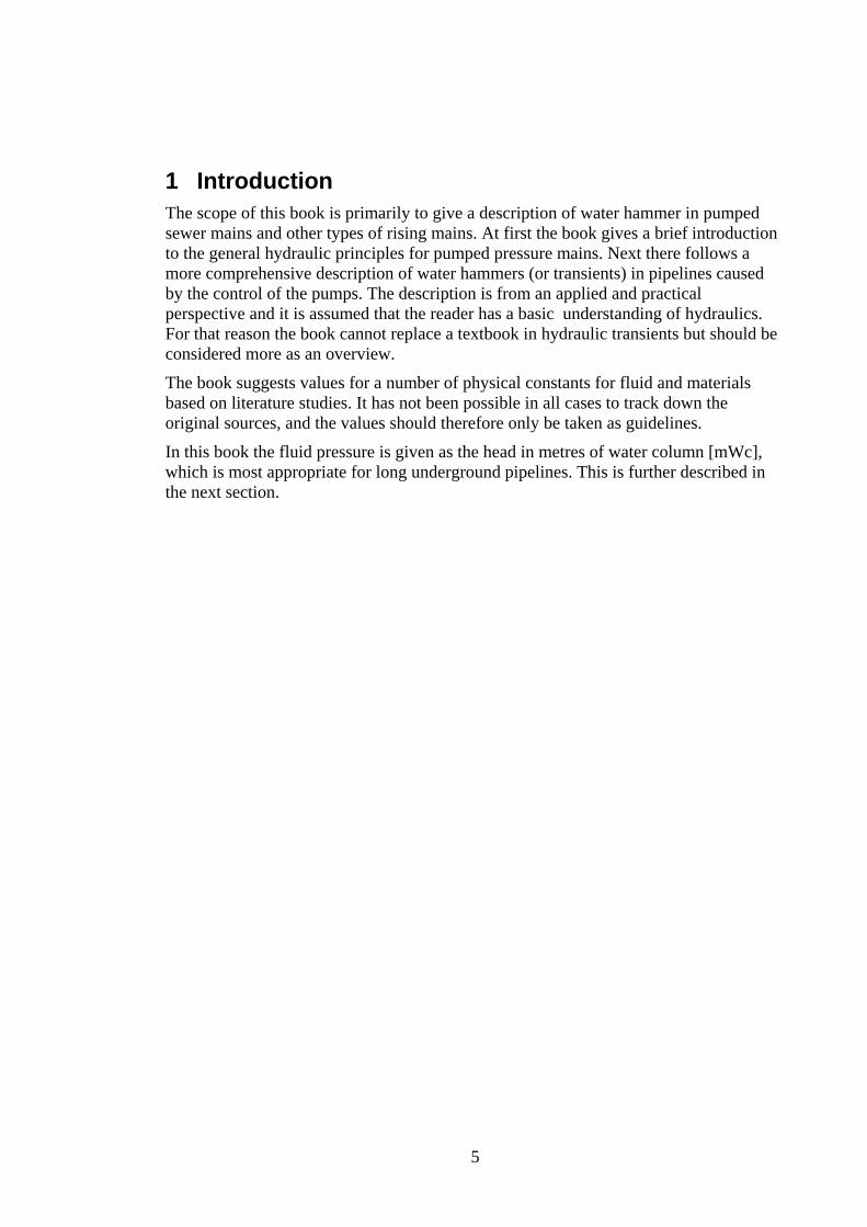
The hydraulic head is the level to which the water surface would rise if a riser pipe was connected to the pipe at the cross section (Figure 2.1).

Figure 2.1 Total head (energy level) and pressure head (hydraulic head) in a pipeline.

6

The total head (energy head) H is defined by

g

VpzH2

2αγ

++= [mWc] (2.2)

The pressure head (hydraulic head) h is defined by

γpzh += [mWc] (2.3)

Both the pressure head and the total head normally refer to an arbitrary reference level (datum). All heads and levels including the length profile of the pipeline should be given relative to the same datum.

The difference between the energy head and the pressure head is the velocity head g

V2

2α

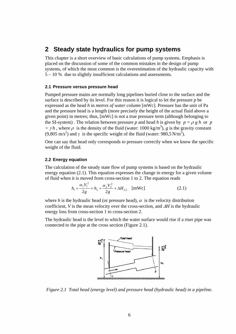
(also called the dynamic head). In practice, there is usually no distinction between hydraulic head and energy head in pump systems because of the relatively small value of the velocity head. In many cases this is a reasonable assumption, but in some cases this can lead to an underestimation of the overall energy losses. In pipelines directly connected to the pump in the pump station (Figure 2.2), velocities are often in the order of 3 - 5 m/s. This means that the velocity head is in the order of 1 m, which may have a significant influence on the design of the pipeline system.

Figure 2.2 Hydraulic head in a pump system

2.3 Duty point

The duty point for a pump system defines the total head and the total flow at steady state. It is found as the head-versus-flow point of intersection between the pump characteristic and the pipeline characteristic (Figure 2.3). At this point the hydraulic lift of the pump equals the total resistance of the pipeline system. This resistance consists of a geometric lift plus the total energy loss.

7

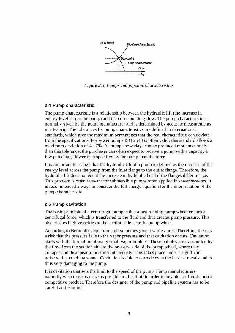
Figure 2.3 Pump- and pipeline characteristics

2.4 Pump characteristic

The pump characteristic is a relationship between the hydraulic lift (the increase in energy level across the pump) and the corresponding flow. The pump characteristic is normally given by the pump manufacturer and is determined by accurate measurements in a test-rig. The tolerances for pump characteristics are defined in international standards, which give the maximum percentages that the real characteristic can deviate from the specifications. For sewer pumps ISO 2548 is often valid; this standard allows a maximum deviation of 4 - 7%. As pumps nowadays can be produced more accurately than this tolerance, the purchaser can often expect to receive a pump with a capacity a few percentage lower than specified by the pump manufacturer.

It is important to realize that the hydraulic lift of a pump is defined as the increase of the energy level across the pump from the inlet flange to the outlet flange. Therefore, the hydraulic lift does not equal the increase in hydraulic head if the flanges differ in size. This problem is often relevant for submersible pumps often applied in sewer systems. It is recommended always to consider the full energy equation for the interpretation of the pump characteristic.

2.5 Pump cavitation

The basic principle of a centrifugal pump is that a fast running pump wheel creates a centrifugal force, which is transferred to the fluid and thus creates pump pressure. This also creates high velocities at the suction side near the pump wheel.

According to Bernoulli's equation high velocities give low pressures. Therefore, there is a risk that the pressure falls to the vapor pressure and that cavitation occurs. Cavitation starts with the formation of many small vapor bubbles. These bubbles are transported by the flow from the suction side to the pressure side of the pump wheel, where they collapse and disappear almost instantaneously. This takes place under a significant noise with a cracking sound. Cavitation is able to corrode even the hardest metals and is thus very damaging to the pump.

It is cavitation that sets the limit to the speed of the pump. Pump manufacturers naturally wish to go as close as possible to this limit in order to be able to offer the most competitive product. Therefore the designer of the pump and pipeline system has to be careful at this point.

8

Problems with cavitation do not occur with the use of submerged pumps; only where the pump is placed above the water surface in the pump sump there is a risk of cavitation. It is good design practice to use a larger pipe diameter on the suction side of the pump compared to the pressure side, and to keep the pipe on the suction side as short as possible.

The lowest allowable pressure on the suction side of the pump under the assumption that the vapor pressure of the fluid is zero, is denoted NPSH (Net Positive Suction Head). This is given by the pump manufacturer. NPSH depends on the flow and is normally given as a graph or a table. Therefore, it is in principle necessary to make a specific analysis of the hydraulic conditions on the suction side of the pump. In sewer systems, where the water is relatively cold, the vapor pressure is negligible compared with the atmospheric pressure, but in principle NPSH must be reduced by the vapor pressure of the fluid.

2.6 Pipeline characteristic

The pipeline characteristic is a graph of the total energy loss in the pipeline as a function of flow (Figure 2.3). Note that it is the energy loss and not the hydraulic head loss being considered. The total energy loss consists of energy losses due to resistances of the pipes and a number of local losses related to the fittings between the pipes. The pipeline characteristic can be calculated by the use of the energy equation from a cross-section in the pump sump to a cross-section in the upstream reservoir, including all components and pipes except the pump.

Usually the major contribution to the pipeline characteristic is the resistance of the main pipeline. Therefore a correct estimate of the hydraulic roughness of the pipe is essential. The roughness given by the pipe manufacturer usually corresponds to the new pipes without sediments and coverings. The experience, especially with plastic pipelines, is that the roughness increases significantly after being in use for some time. However, there are also examples where concrete pipelines have attained a lower roughness after some years, probably because of wear from sediments. Table 2.1 gives some guidelines on hydraulic roughness for sewer mains in practice.

Table 2.1. Hydraulic roughness k in pressure mains ( intended only as a guide) Type of pipe Roughness

New pipe without coverings mm

Roughness Old pipe with coverings Mm

Ductile iron 0.1 – 0.2 0.5 – 1.0

Galvanized steel pipes 0.1 – 0.3 0.5 – 3.0

Concrete pipes 0.3 – 1.5 -

uPVC and PE plastic 0.01 - 0.05 0.15 – 0.6

Reinforced polyester 0.02 – 0.05 0.15 – 0.6

The hydraulic roughness in sewers is not well defined. It should be mentioned that British experience (Casey, 1992) shows that the hydraulic roughness in sewers caused

9

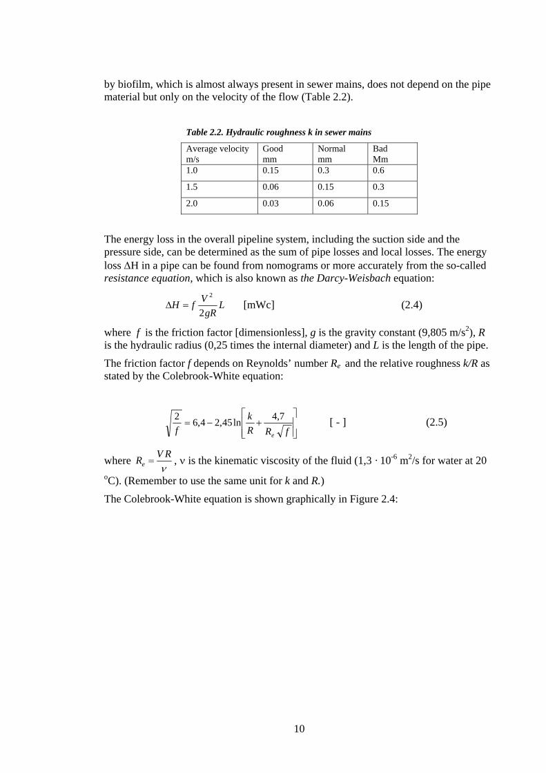
by biofilm, which is almost always present in sewer mains, does not depend on the pipe material but only on the velocity of the flow (Table 2.2).

Table 2.2. Hydraulic roughness k in sewer mains

Average velocity m/s

Good mm

Normal mm

Bad Mm

1.0 0.15 0.3 0.6

1.5 0.06 0.15 0.3

2.0 0.03 0.06 0.15

The energy loss in the overall pipeline system, including the suction side and the pressure side, can be determined as the sum of pipe losses and local losses. The energy loss ΔH in a pipe can be found from nomograms or more accurately from the so-called resistance equation, which is also known as the Darcy-Weisbach equation:

LgR

VfH2

2

=Δ [mWc] (2.4)

where f is the friction factor [dimensionless], g is the gravity constant (9,805 m/s2), R is the hydraulic radius (0,25 times the internal diameter) and L is the length of the pipe.

The friction factor f depends on Reynolds’ number Re and the relative roughness k/R as stated by the Colebrook-White equation:

⎥⎥⎦

⎤

⎢⎢⎣

⎡+−=

fRRk

f e

7,4ln45,24,62 [ - ] (2.5)

where νRVRe = , ν is the kinematic viscosity of the fluid (1,3 · 10-6 m2/s for water at 20

oC). (Remember to use the same unit for k and R.)

The Colebrook-White equation is shown graphically in Figure 2.4:

10

Figure 2.4. The friction factor as a function of Reynolds’ number and the relative roughness

Because the friction factor is implicitly given in the Colebrook-White equation, it is necessary to use iteration to find f. This can be done by rewriting the equation to

27.4ln45,24,6

2

⎟⎟

⎠

⎞

⎜⎜

⎝

⎛

⎥⎥⎦

⎤

⎢⎢⎣

⎡+−

=

fRRk

f

e

[ - ] (2.6)

The iteration takes place in the following way: The starting point is to guess a value of f, for example 0,001. This value is inserted on the right-hand side (together with values of Reynolds' number and the relative roughness) and we then obtain a new value of f. This new value is now inserted on the right hand-side, etc., etc. After 4 - 5 iterations a constant value is achieved. This procedure is easy to carry out in a spreadsheet program (for example Microsoft Excel), where the equation can be inserted into one cell and copied to the cells below.

The energy losses at inlets, outlets, bends, valves, etc., should be treated as local losses and calculated from

g

VH2

2

ξ=Δ [mWc] (2.7)

where ζ is the local-loss coefficient [dimensionless].

11

The local-loss coefficients for the individual components are normally given by suppliers. Values for characteristic bends, contractions, etc., can be found in textbooks and handbooks.

Often the flow Q is introduced in the single-loss equation, which gives

2

2

2gAQH ξ=Δ [mWc] (2.8)

where A is the cross-section area of the pipe [m2].

From this equation it is clear that the value of ζ relates to the cross-section area.

It is common use for fittings, for example valves, that ζ corresponds to the cross-section area of the flange of the fitting, even though the velocity, which in a proper sense is the cause of the energy loss, is much larger inside the fitting than at the flange. This is compensated by the use of a much larger value of ζ. If we, for example, have a ζ−value of 20 for a seat valve, we know that somewhere inside the fitting we have a contraction with a cross-section significantly smaller than the cross-section of the flange.

Because of the reasons mentioned above we see that it is wrong simply to add together the values of ζ in a pipeline system unless all diameters of pipes and fittings are equal.

For a given flow Q all the energy losses are added together to give the overall energy loss ΔΗtotal. As a good approximation ΔΗtotal is proportional to Q2:

ΔΗtotal = K Q2 [mWc] (2.9)

where K is a constant called the specific resistance of the pipeline system.

A straightforward method for the determination of the pipeline characteristic is to choose an arbitrary value Q0 for the flow. For this flow the corresponding total energy loss ΔΗ0 in all pipes and fittings are calculated. Now K can be determined, and equation (2.9) can then be used to draw up the pipeline characteristic for various values of Q.

2.7 Self-cleansing

Sewage contains particulate matter, which may deposit in the pipelines. To ensure self-cleansing a minimum flow velocity is required when the pump is running. Experience shows that a minimum bed shear stress of approximately 3 - 4 Pa is needed to enable transport of sediments like sand and gravel along the bottom. This holds for the so-called combined sewer systems, which carry both sewage and rainwater. For separate rainwater systems a minimum shear stress of 2 Pa is required.

The bottom shear stress τ can be determined from

τ = γ R I [Pa] (2.10)

where γ is the specific weight of the fluid (980.5 N/m3 for water), R is the hydraulic radius (0.25 times the internal pipe diameter) and I is the energy loss per unit length of the pipe.

12

A minimum velocity requirement is a practical alternative to using bed shear stress. As a rule of thumb, the minimum velocity is 0.6 to 0.8 m/s.

As mentioned earlier the depositions also have an influence on the hydraulic roughness of the pipes.

2.8 Air pockets

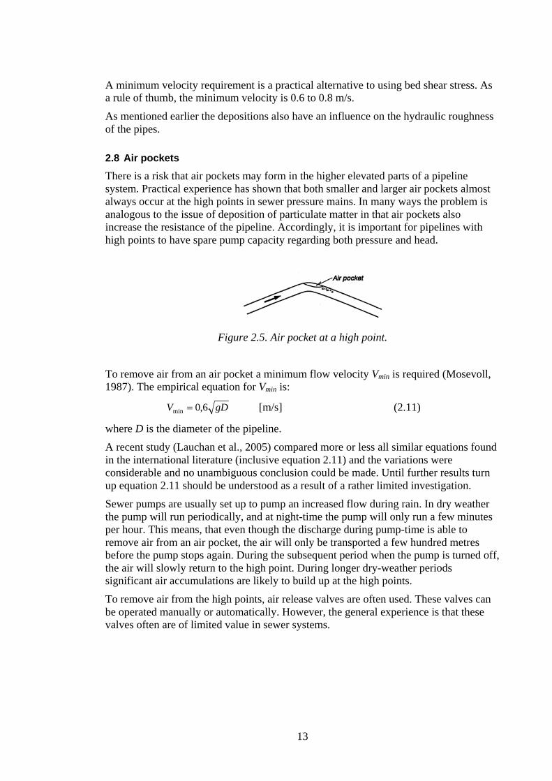
There is a risk that air pockets may form in the higher elevated parts of a pipeline system. Practical experience has shown that both smaller and larger air pockets almost always occur at the high points in sewer pressure mains. In many ways the problem is analogous to the issue of deposition of particulate matter in that air pockets also increase the resistance of the pipeline. Accordingly, it is important for pipelines with high points to have spare pump capacity regarding both pressure and head.

Figure 2.5. Air pocket at a high point.

To remove air from an air pocket a minimum flow velocity Vmin is required (Mosevoll, 1987). The empirical equation for Vmin is:

gDV 6,0min = [m/s] (2.11)

where D is the diameter of the pipeline.

A recent study (Lauchan et al., 2005) compared more or less all similar equations found in the international literature (inclusive equation 2.11) and the variations were considerable and no unambiguous conclusion could be made. Until further results turn up equation 2.11 should be understood as a result of a rather limited investigation.

Sewer pumps are usually set up to pump an increased flow during rain. In dry weather the pump will run periodically, and at night-time the pump will only run a few minutes per hour. This means, that even though the discharge during pump-time is able to remove air from an air pocket, the air will only be transported a few hundred metres before the pump stops again. During the subsequent period when the pump is turned off, the air will slowly return to the high point. During longer dry-weather periods significant air accumulations are likely to build up at the high points.

To remove air from the high points, air release valves are often used. These valves can be operated manually or automatically. However, the general experience is that these valves often are of limited value in sewer systems.

13

3 Water hammer and cavitation in pumped mains Water hammer (or transient) is a wave phenomenon that occurs in the liquid in a pipeline when a pump starts or stops or when a valve closes or opens. In principle any change in flow velocity can cause water hammer. In some cases the effect results in a hammering noise from the pipeline, which is why it is called water hammer. Often water hammer is the strongest physical load a pipeline is exposed to. Typical damages are breaks in the pipes over shorter or longer distances. Numerable examples of this kind of damages can be given.

3.1 Water hammer

The description of water hammer from a physical point of view takes its starting point in Newton's second law, which expresses that force equals mass times acceleration. This means that severe water hammer occurs where large masses of fluid are given high accelerations.

Water hammer is closely connected with other wave phenomena, for example the propagation of sound waves. An essential component of water hammer is the reflection of waves at the end of the pipeline regardless of whether the end is open or closed. A negative pressure wave, which occurs for example when a pump shuts down, will be reflected at the end of the pipeline and return as a positive wave.

3.2 Cavitation

If no specific precautions are taken, the water hammer caused by pump start-up or shut-down may cause the pressure to fall below the vapor pressure of the fluid. If this happens the continuity of the fluid is broken, or in other words - the fluid is boiling. This is cavitation (see also Section 2.5).

Table 3.1 shows the vapor pressure of water as a function of the temperature. It shows that the vapor pressure in pumped mains is negligible compared to the normal barometric pressure of 10.13 mWc for temperatures below 200C.

Table 3.1. Vapor pressure PD [mWc] of water as a function of temperature T [0C].

T 0C 0 10 20 30 40 50 60 70 80 90 100

PD mWc 0.06 0.13 0.23 0.42 0.73 1.23 1.99 3.12 4.75 7.01 10.13

Often the fluid contains dissolved gasses. For example, water is most often highly saturated with atmospheric air. If the pressure reduces because of water hammer, the fluid can become supersaturated with air, which is then released as small bubbles. The small bubbles then accumulate and form large bubbles. Since such accumulations cannot be dissolved as soon as they are released, the effect of water hammer can result in a net creation of air or gas pockets. Pumping of fluids with a high content of dissolved gasses, for example carbonated beverages, requires special analysis.

14

A more profound description of water hammer is found in the literature. A good starting point is Wylie and Streeter (1983).

3.3 Example of measurement of water hammer

Figure 3.1 shows the length profile of an approximately 3 km long sewer pressure main in western Denmark. Measurements of pressure were taken close to the pump station as indicated.

Figure 3.1 Length profile of sewer pressure main (Larsen and Binder, 1984).

Figure 3.2 shows the pressure head as a function of time over a period of 210 seconds (3½ minutes).

Figure 3.2 Pressure head in pipeline close to pump station (Larsen and Binder, 1984).

At the start (t = 0) both pumps are turned off. Then one pump is turned on, and shortly after the second is turned on too. The figure shows that the pressure is considerably higher than the steady state pressure during the acceleration period due to a reduced pump performance.

15

Both pumps are shut down approximately 1 minute after start-up, and the pressure drops to a negative value of approximately - 2 mWc. This negative pressure has the effect that a certain flow continues through the pump and that the non-return valves stay open. About 0.5 minutes after pump shut-down the pressure rises sharply to a high of approximately 75 mWc. After this follows several repeats of the drop-rise sequence, but with decreasing amplitude.

From these measurements it is seen that the pressure in the pipeline varies by almost 80 mWc, which is much more than acceptable for the actual uPVC pipe being used, with respect to the risk of failure because of fatigue. Based on the results of a subsequent computer simulation an air chamber was installed at the pump station. The air chamber reduced the pressure fluctuation to an acceptable level.

The measurements also showed some short periodic pressure fluctuations (between 12 and 30 seconds), which indicated that cavitation occurred somewhere in the pipeline. This assumption was supported by a strong noise at the end of the pipeline near the reservoir. Computer simulation later confirmed that cavitation occurred near the first high point in the pipeline.

Figure 3.2 clearly illustrates how the water hammer is more damped when the pump is running compared to when the pump is turned off.

16

4 The influence of water hammer on the design of pipelines

Because water hammer creates the most severe forces on the pipelines, the selection of pipe material and the determination of the thickness of the pipe wall depend primarily on the stresses from the transients. However, it is rare that internal water pressure is the one and only factor in the dimensioning. Other factors often play an important role, for example external water and soil pressure including traffic load.

The scope of this publication is the hydraulics of transients; a complete and detailed description of the structural design of pipelines will not be given here. In the following text only some general principles will be presented together with a few examples.

4.1 Effect of maximum and minimum internal pressure

In a circular pipeline with an internal pressure p a ring stress σt emerges. This stress can be expressed:

e

pDt 2

=σ [MPa] (4.1)

where D is the pipe diameter and e is the thickness of the pipe wall.

As long as the pressure is positive it is obvious that σt should be less than the design (permissible) strength for the pipe material. For static loads the design strengths for various materials are given in Table 4.1.

Table 4.1 Design stress for various pipe materials

Pipe material

Design stress

[MPa]

Steel 150 – 180

Ductile iron 200 – 250

Reinforced concrete 0

Asbestos concrete 5 – 8

PVC (polyvinylchloride) 20oC 10 – 12.5

PEL (polyethylene low density) 20oC 3

PEM (polyethylene medium density) 20oC 5

PEH (polyethylene high density) 20oC 5 – 6

PP (polypropylene) 20oC 5

GRP (glass reinforced polyester) > 100

GRE (glass reinforced epoxy) > 100

17

The design stresses given in Table 4.1 incorporate a safety factor in the order of a magnitude of 2.

If a negative pressure in the liquid occurs, resulting in a positive stress in the pipe wall, the situation is more complex. In this case there is a risk of collapse or buckling. The maximum permissible stress pE in respect to buckling is:

For a pipe restrained in the length direction

3

3

212

DepE μ−

= [ΜPa] (4.2)

For an unrestrained pipe

EDepE 3

32= [MPa] (4.3)

where μ is the Poisson’s ratio and E is the elastic modulus (Young’s modulus) of the pipe material.

Because collapse or buckling in principle depends on the elastic modulus and not on the design stress of the material, it is essential to incorporate a safety factor (with a value of approximately 2) to achieve the permissible buckling stress.

The equations given above are from the theory of thin-walled pipes and do not take into account the influence of soil pressure. Guidelines for the design of thick-walled pipes are found in the literature. Low pressure from water hammer caused by pump start-up and shut-down are relative short-lived and one should therefore apply the short-term elastic modulus for evaluation of collapse and buckling caused by water hammer. This stands in contrast to long-term impacts from for example external water and soil pressure. In these cases the long-term elastic modulus should be used. Consequently, a precise evaluation of combined short- and long-term influences on plastic pipelines is difficult and uncertain.

It should be emphasized that the structural design of plastic pipes also should include an estimate of the deformation of the pipe. If the cross-section of the pipe has an initial deviation from circular, this should be considered as well.

Example:

Let us consider the strength of a PN6 (6 bar) unrestrained uPVC pipe with an outer diameter of 500 mm and the following data: Wall thickness e = 14.6 mm Average diameter D = 485.4 mm Short-term elastic modulus E = 3.3 106 kPa.

18

The critical buckling pressure is:

mWckPapE 186.1794854.0

0146.0103.323

36

≈=⋅⋅⋅

=

With a safety factor γm = 2 the design buckling pressure will be around – 9mWc, which is near to (but less than) full vacuum ( - 10,1 mWc).

For the same pipe in pressure class PN10 (10 bar) we have e = 25.4 mm and an average pipe diameter of D = 474.6 mm. In this case the critical buckling pressure is:

mWckPapE 1001016474.0

0254.0103.323

36

≈=⋅⋅⋅

=

Including the safety factor gives a design buckling pressure of approximately - 50 mWc, which means that the pipe should be able to resist full vacuum (cavitation) as well as some external pressure from outside.

This example only covers the strength of the pipe. In practice also the deformations should be considered.

4.2 Fatigue

In pumped sewer pressure mains pumps normally start-up and shut-down at least once in an hour. With a life of 50 years this gives about 500 000 stops. As shown earlier (Figure 3.2) each stop generates a number of pressure fluctuations. In total the pipe will go through somewhere between 106 to 107 fluctuations in its lifetime.

It is well-known that most materials show a decreasing strength when the load is pulsating. If the stress in the pipe wall varies between 0 and σmax in each pulse, the tensile strength can be graphed against the number of pulses in a so-called Whöler-diagram. Figure 4.1 shows an example of a Whöler-diagram for uPVC

Figure 4.1 Whöler-diagram for uPVC (Stabel, 1977)

19

In practice the stress in the pipe wall will fluctuate around an average value σm with an amplitude σa as shown in Figure 4.2.

Figure 4.2 Definition of mean stress σm and stress amplitude σa

The effect of a fluctuating stress on the material is read from a Goodman-diagram (Figure 4.3).

Figure 4.3 Goodman-diagram for uPVC

From the example in Chapter 3 (Figure 3.2) it is obvious that the fluctuations do not have constant amplitude. This problem can be solved by use of Miner’s law, which expresses:

20

+++=4

3

2

2

1

1

Nn

Nn

Nn

Nn

n

n … (4.4)

where ni is the number of loads at stress level i that do not lead to failure, and Ni is the number of loads at stress level i that lead to failure.

Miner’s law was first established for aluminium and its validity has never been proved in depth for plastic materials, so the law must be treated with caution. However, a certain practice exits with direct or indirect reference to Miner’s law after which it is justifiable to accept higher loads for rare events like power break down.

4.3 Practice for pipe design

Denmark

For plastic pipes the principles mentioned above are simplified to include only maximum stresses and maximum amplitudes. For sewer pressure mains made of uPVC it is recommended (Wavin, 1993; Uponor, 1997) that the maximum permissible long-term stress of 10 N/mm2 is increased to 12.5 N/mm2 (because of temperature), and that the amplitude of the fluctuations should be less than 30 % of the 10 N/mm2. For a PN6 (bar) pipe this means that the maximum pressure in connection with transients is 75 mWc, and that the maximum fluctuation (twice the amplitude) is 36 mWc from lowest to highest value.

Sweden

In Sweden no standards exists. VAV recommends (VAV, 1988) that a safety factor of at least 3 for plastic pipelines should be used. Concerning fatigue it is recommended that the stress amplitude should be less than 20 % of the maximum pressure for the pipe. Thus, the Swedish recommendations seem more conservative than the Danish.

21

5 Basic principles for water hammer

Water hammer is a wave phenomenon similar to sound waves, for example. The central issue is that the change in pressure and flow moves with a maximum velocity many times higher than the velocity of the flow.

5.1 Celerity of the pressure wave

The wave celerity (another word for velocity) in pipelines will most often be more than 200 – 300 m/s, but it will always be lower than the wave celerity of sound in the fluid (in water the celerity of sound is close to 1450 m/s). The celerity for pressure changes is the same as the celerity for velocity changes and depends in principle on the density of the fluid and the elasticity of the fluid and the pipe.

The elasticity of the pipe depends primarily on the thickness of the pipe and the elasticity modulus of the pipe material. Also the restraint in the length direction has some influence. It is well known that material that expands in one main dimension will tend to contract in the two other main dimensions. This tendency is more pronounced in plastic materials with relatively high Poisson’s ratios. The elasticity of the pipe wall therefore depends on whether the pipe can move in the length dimension. A pipeline with flexible joints like for example uPVC pipes are not considered restrained in contrast to for example PE pipes with welded joints buried in the ground.

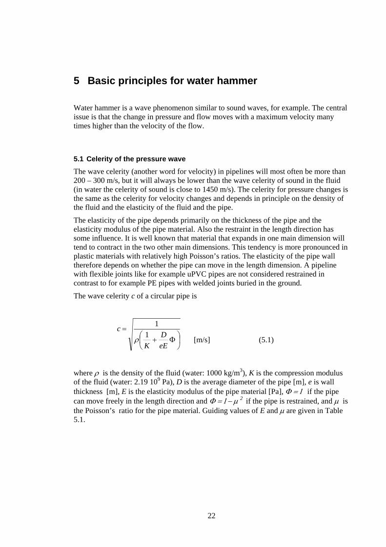
The wave celerity c of a circular pipe is

⎟⎠⎞

⎜⎝⎛ Φ+

=

eED

K

c1

1

ρ [m/s] (5.1)

where ρ is the density of the fluid (water: 1000 kg/m3), K is the compression modulus of the fluid (water: 2.19 109 Pa), D is the average diameter of the pipe [m], e is wall thickness [m], E is the elasticity modulus of the pipe material [Pa], Φ = 1 if the pipe can move freely in the length direction and Φ = 1− μ 2 if the pipe is restrained, and μ is the Poisson’s ratio for the pipe material. Guiding values of E and μ are given in Table 5.1.

22

Table 5.1 Guiding values for pipe materials (always to be confirmed with the supplier)

Pipe material Elasticity modulus E

106 MPa

Poisson’s ratio μ

Steel 210 0.3

Ductile iron 100 – 150 0.25

Concrete 30 – 60 0.2

uPVC plastic short-term 3.3 0.4

HDPE plastic short-term 0.8 0.4

For plastic materials the elasticity modulus depends on the duration of the load. Therefore different values should be applied for different types of loads. For steady loads, such as external water and soil pressure, long-term values are used, whereas short-term values are relevant for water hammer.

Practical experience is that the wave celerity in buried pipes is not influenced by pressure from soil under normal conditions. The reason is probably that deformations caused by transients are too small to mobilize any soil pressure.

If the fluid contains free gas bubbles (for example air) the elasticity of the fluid will increase and the wave celerity will reduce. This will again reduce the water hammer. This effect should be taken into account in the dimensioning, and it could be the reason for measurements showing lower pressure fluctuations than computer simulations.

5.2 Joukowsky’s equation

From Newton’s second law we understand that force (pressure times area) is the result of a mass being accelerated. In this connection the wave celerity c stands for the mass per unit time which is accelerated. The acceleration is caused by pumps, valves, etc. Therefore it is likely that stiff systems with high wave celerity will give higher force and pressure. The Joukowsky equation expresses the rise in pressure Δp caused by a change in velocity ΔV:

Δp = ± c ρ ΔV [Pa] (5.2)

If we use hydraulic head h instead of pressure, we obtain:

Vgch Δ±=Δ [mWc] (5.3)

where ρ is the density of the fluid (water: 1000 kg/m3) and g is the gravity constant (9,805 m/s2).

23

The sign of Δp or Δh depends on the direction. If we close a valve we get a pressure rise at the upstream side of the valve and a pressure drop on the downstream side.

Example

In a steel pipe with an internal diameter of 100 mm water is flowing with a velocity of 0,5 m/s. Suddenly a valve is closed, and we want to estimate the pressure rise.

The density of the water is 1000 kg/m3. The thickness of the wall is 3 mm and the elasticity modulus E is 210 109 Pa . The pipe is not restrained and can move freely in the length direction.

The average pipe diameter D = (100 + 106)/2 = 103 mm.

The wave celerity is calculated:

smc /12701

10210003.0103.0

1019.211000

1

99

=

⎟⎟⎠

⎞⎜⎜⎝

⎛

⋅+

=

Now the Joukowsky equation gives

Δp= ±1270 1000 ⋅ 0.5 = ±635 106 Pa

or

Δh= ±(1270/9.805) ⋅ 0.5 =± 65 mWc

The change in pressure is positive at the upstream side of the valve and negative at the downstream side.

The estimated changes are the changes immediately after the close of the valve. How the pressure will develop in time from this situation cannot be found from the Joukowsky equation. This requires computer simulations.

It should be mentioned that a pressure drop of 65 mWc can only take place if cavitation does not occur. Thus, the example indicates that fast-closing valves are likely to cause cavitation.

5.3 Reflection of water hammer

Figure 5.1 illustrates the variations in pressure and how the flow propagates forwards and backwards in the pipeline after the closure of the valve. For simplicity any friction is neglected. The time it takes for the wave to move through the pipe is

cLT =0 [s] (5.4)

where L is the length of the pipeline and c is the wave celerity.

24

The reflection time Tf is defined as the time it takes for the pressure wave to move forward and backwards once in the pipe. This gives

Tf = 2 T0

Immediately after the closure of the valve a positive pressure wave starts moving against the flow direction towards the open end of the pipe. At the time t = T0 the pressure has changed + Δp everywhere in the fluid and the velocity is nil. This is an unstable situation, and the positive pressure will press the water out of the pipe by starting a wave going backwards in the pipe (towards the left in Figure 5.1). At the left side of the front the pressure is nil and the velocity is – V. Figure 5.1 shows how the wave propagates back and forth in the pipe.

To understand water hammer it is essential to realize that the wave is reflected from a closed end as well as an open end of the pipe. Reflection often plays an essential role in relation to transients in pipelines.

In theory the waves continue forever. In the real world friction will gradually damp out the waves. The principles shown in Figure 5.1 will usually be valid during the first one or two reflection periods. The immediate effect of closing a valve can be found from the Joukowsky equation. Because of the reflection the pressure wave will return at the valve some time later with the opposite sign. Consequently, the fast closure of a valve can provoke cavitation on both sides of the valve.

25

Figure 5.1 Principle of water hammer reflection

5.4 Reflection in joints between pipes in series

Pipe systems will often be composed of a number of various pipes in series. Reflection in relation to water hammer will take place at all points where we have a change in diameter or in wave celerity. When the flow moves from a small pipe into a large pipe

26

the reflection is large, in some cases almost 100 %. The transmission factor k for the transmitted pressure wave over a joint can be found from (Wylie and Streeter, 1983):

21

121

2

AcAck

+= [ - ] (5.5)

where c1 and A1 are the upstream wave celerity and cross-section area, respectively, and c2 and A2 are the downstream wave celerity and cross-section area, respectively.

In sewer pump systems the pipes in the pump station are usually steel pipes, whereas the main transport pipe is usually in plastic (Figure 5.2). It is obvious from the Joukowsky equation that the pressure rise will be much higher in the steel pipe than in the plastic pipe.

Figure 5.2 Reflection in pump station

The situation for the pipeline illustrated in Figure 5.2 is that a pressure change in the steel pipe caused by a velocity change will be partly reflected at the joint between the two pipes and sent backwards towards the pump. The part of the pressure wave that continues in the plastic pipe will have a magnitude that can be determined from the Joukowsky equation for the plastic pipe with the actual velocity change, which is lower here because of the larger cross-section area.

The important issue is that high local transients in the pump station do not penetrate into the main plastic pipe.

27

6 Water hammer in pumping mains Transients occur at pump start-up and shut-down. Running centrifugal pumps have a significant damping effect on transients. Therefore the starting of pumps in general cause only minor problems compared to the shutting down. Also, the fact that most pumping mains have non-return valves installed in the pump stations contribute to the larger problems with transients at pump shut-down.

6.1 Pump start-up

Transients at pump start-up occur when the start-up lasts for a shorter period than the acceleration of the water column in the pipe. A rough estimate for the time of acceleration is the reflection time Tf = 2 L/c. General experience is that a pipeline attains its steady state flow in less than one or two times Tf. A distinction between short and long pipes is useful in this context. A short pipe is a pipe where the acceleration period is shorter than the start-up of the pump. A long pipe is a pipe where the period of acceleration is considerably longer than the start-up of the pump. By definition short pipes do not cause water hammer problems.

Figure 6.1 Water hammer at pump run-up

Figure 6.2 shows the progress of a typical pump start-up at a point just downstream the pump. Point (1) is the situation just before the pump begins to rotate, with the non-return valve being closed and the pressure head corresponding to the geometric head. Point (2) denotes the situation just after the pump has come to its full speed. This is the intersection point between the pump characteristic and the characteristic for the transient. The characteristic for the transient is a straight line through point (1) and with a slope α given by the Joukowsky equation:

Vh Δ=Δ α or QAg

ch Δ=Δ [mWc] (6.1)

28

where Δh is the change in head, ΔV is the change in velocity, c is wave celerity, g is the gravity constant, and ΔQ is the change in flow. Figure 6.1 shows that the head is higher and the flow is lower during the acceleration phase. Due to friction in the pipe the head will increase slightly after pump start-up until the time marked (3), when the initial wave returns from the upstream end of the pipe. The system has reached steady state and the duty point already after one or two reflections.

As illustrated in the figure, the maximum head can easily be found graphically with a reasonable accuracy without use of computer programs.

6.2 Pump shut-down

Transients at pump shut-down are normally much more complicated and critical than at pump start-up. Most cases of pipe bursts occur at pump shut-down. For larger systems thorough investigations including computer simulations are needed.

As mentioned in the preceding section it is important to distinguish between long and short pipes and to realize that transients only occur in long pipes. The pump shut-down lasts from a fraction of a second to a few seconds depending on the size and speed of the pump and the load on it. A steel pipe with a length of 10 m is a short pipe, because a pressure wave will return to the pump with a negative sign after less than 2 milliseconds, whereas a pressure wave in a 3-kilometer long plastic pipe will first return after around 20 seconds.

When a pump shuts down the rotation reduces rapidly, but it is important to understand that a stopped pump does not imply that the flow also stops. Most pumps have a considerably open passage, which allows a continuation of the flow if a pressure drop over the pump occurs. The non-return valve prevents the flow going backwards through the pump.

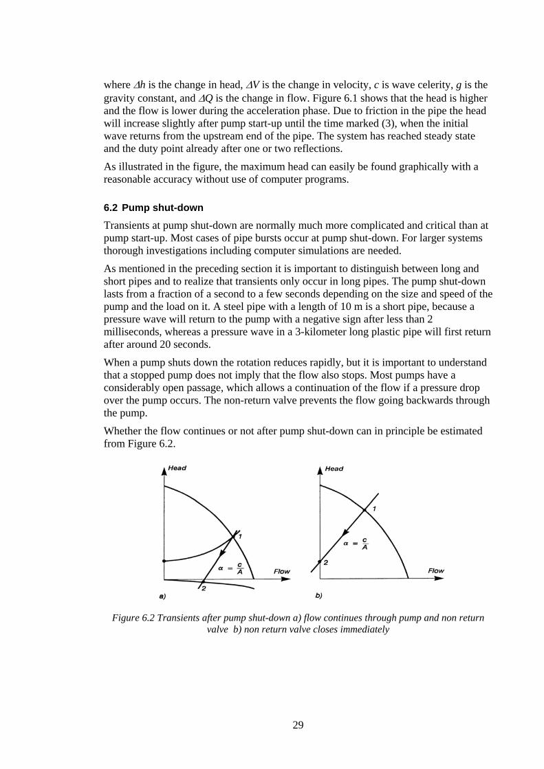
Whether the flow continues or not after pump shut-down can in principle be estimated from Figure 6.2.

Figure 6.2 Transients after pump shut-down a) flow continues through pump and non return

valve b) non return valve closes immediately

29

Situation (1) is immediately before pump shut-down, and situation (2) is just after the rotation has stopped. Again the characteristic of the transient is a line through point (1) and with a slope according to the Joukowsky’s equation. The characteristic of the stopped pump is a parabola equivalent to a head-loss equation for an orifice. If the intersection between the characteristic of the transient and the ordinate axis shows a positive head (Figure 6.2b), the non-return valve needs to close to avoid backwards flow. An intersection with a negative head (Figure 6.2a) indicates that the non-return valve is still open and that flow continues through the pump.

The two cases are different in that way that in one case the transient is controlled by a drop in flow and in the other by a drop in pressure.

The description given above is simplified to some extent and should primarily be used to investigate whether the non-return valve will close or not. The progress in flow and pressure through the stopping pump cannot be estimated accurately . The minimum pressure can only be roughly estimated (underestimated) from the figure.

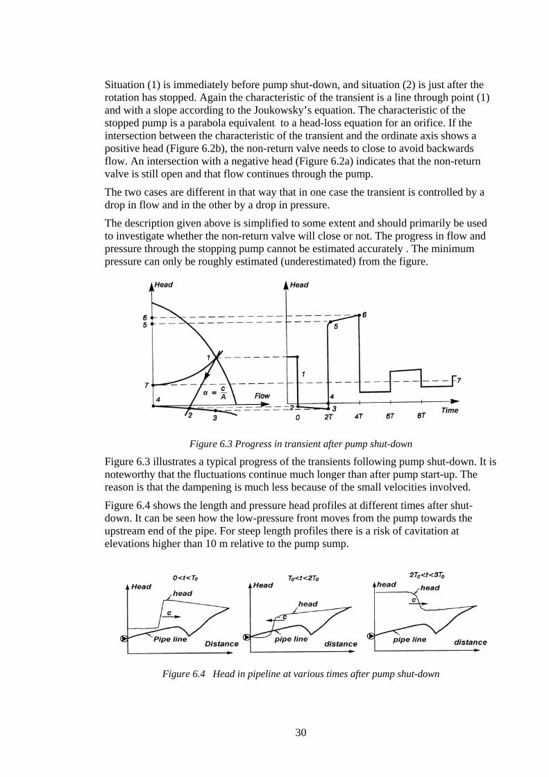
Figure 6.3 Progress in transient after pump shut-down

Figure 6.3 illustrates a typical progress of the transients following pump shut-down. It is noteworthy that the fluctuations continue much longer than after pump start-up. The reason is that the dampening is much less because of the small velocities involved.

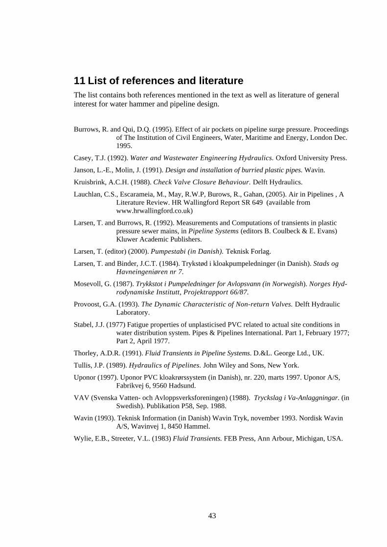
Figure 6.4 shows the length and pressure head profiles at different times after shut-down. It can be seen how the low-pressure front moves from the pump towards the upstream end of the pipe. For steep length profiles there is a risk of cavitation at elevations higher than 10 m relative to the pump sump.

Figure 6.4 Head in pipeline at various times after pump shut-down

30

6.3 Inertia of the pump

A running pump contains kinetic energy from rotation of the pump wheel, shaft, clutch and motor. A part of the fluid in the pump also contributes to kinetic energy. The kinetic energy Ekin of a rotating system is

2

21 ωIEkin = [J]

where I is the total moment of inertia and ω = 2 π n is the angular velocity of the rotation with n being the number of revolutions per unit time.

The mechanical power P delivered by the motor via the clutch to the pump shaft is

ηγ HQP = [W]

where γ is the specific gravity of the fluid (water: 9,805 kN/m3), Q is the flow, H is the head of the pump and η is the mechanical efficiency of the pump.

A rough estimate of the duration of the shut-down period can now be found from

HQI

PEt kin

γηω 2

21

==Δ [s]

This estimate is only an order of magnitude because the flow, the head and the efficiency vary during the shut-down period. The real value is typically 2–3 times smaller.

The moment of inertia of motor and pump is usually supplied by the manufacturer. The literature gives some empirical equations, which can be used if information is not available. Thorley (1991) presents the following equation for centrifugal pumps and motors:

Centrifugal pumps: 9556.0

03768.0 ⎟⎠⎞

⎜⎝⎛=

NPI p [kg m2]

Motors: 48.1

0043.0 ⎟⎠⎞

⎜⎝⎛=

NPI m [kg m2]

where P is the mechanical power in kW and N is the rpm in 1000 revolutions per minute.

Example

Flow: 0.25 m3/s Head: 70 m Efficiency: 0.72

31

Rpm: 1450 per minute

The power can be found as

kWP 238100072.0

70805.9100025.0=

⋅⋅⋅⋅

=

The moment of inertia for the pump:

29556.0

3 4.245.1

23803768.0 mkgI p =⎟⎠⎞

⎜⎝⎛=

The moment of inertia for the motor:

248.1

2.845.1

2380043.0 mkgI m =⎟⎠⎞

⎜⎝⎛=

Thus the total moment of inertia is Itotal = 2.4 + 8.2 kg m2= 10.6 kg m2 and this value should only be taken as rough estimate, as mentioned.

The importance of the inertia of the pump is most varying. As already described the important issue is the ratio between the duration of the shut-down period and the reflection time of the pipeline. Figure 6.5 shows the length profile of a pipeline and the pressure head 5 seconds after pump shut-down in two situations: one with a low (0.1 kg m2) moment of inertia and one with a high (1.0 kg m2) moment of inertia.

Figure 6.5 Length profile of the pressure wave in a pipeline 5 seconds after pump shut-down in systems with low moment of inertia (0.1 kg m2) and high moment of inertia (1.0 kg m2).

For long plastic pipes (for example sewer mains) the moment of inertia of the pump can often be neglected. This is not the case for short steel pipes in industrial surroundings.

32

7 Precautions against water hammer at pump shut-down

As explained in the previous chapter, water hammer is caused by accelerations of flow in the pipeline. Naturally the precautions against water hammer are attempts to reduce the changes in flow velocity as much as possible. The most well-know methods are described in the following.

7.1 Revolution control of pumps

Revolution (or speed) control of the pump motor is the most efficient and flexible method for reducing water hammer. The standard method is the use of a so-called ramp by which the revolution of the pump varies linearly with time (the speed is ramped-down). As the length (in time) of the ramp can usually be fully adjusted, an almost total elimination of the water hammer is possible.

It should be mentioned that a linear shut-down of the pump is not optimal from a theoretical point of view, because the pump head varies quadraticly to pump speed Thus, a shut-down ramp where the speed follows the square root of the time can reduce the necessary ramp length.

The only serious weakness of the use of speed control is the problem with power failure. For most countries statistics of the so-called LOLP (Loss-of-Load-Probability) for the power network are available. In Denmark the LOLP on the 10–20 kV network is about 0,5 to 1 per year, but for a local network the value is higher.

7.2 Flywheel

As described in the preceding chapter the pump inertia can have a significant effect on the water hammer especially in the case of short pipelines. The moment of inertia can be increased by installing a flywheel, which in many ways is an excellent way of reducing water hammer. However, nowadays flywheels are uncommon because they take space and are expensive. Also, the start-up procedure of the motor is more complicated when a flywheel is involved.

7.3 Air chamber

Air chambers (or air vessels) are frequently used to reduce water hammer caused by pumps and valves (Figure 7.1). They come in sizes from a few cubic centimeters to several hundred cubic metres.

The basic principle is that the compressed air in the air chamber acts as a kind of pump the first seconds after pump shut-down. The compressed air slows down the loss of velocity in the main pipe, which reduces water hammer. The disadvantage is that the pressure is kept high on the upstream side of the pump, forming a pressure gradient backwards through the pump, which will force the non-return valve to close faster and this can sometimes damage the valve.

33

Figure 7.1 Air chamber with compressor

A larger air chamber needs a compressor to keep a constant air content in the tank. Smaller air chambers can instead have the air in a closed rubber membrane.

Air chambers are pressure tanks usually made of steel, and they have to comply with strict safety requirements.

7.4 Surge tanks

A surge tank (or surge tower) is in principle an air chamber open to the atmosphere. Thus, the chamber should be higher than the working head of the pump plus the maximum head variations caused by pump run-up and shut-down. Surge tanks are mostly used for large pipelines with low geometric heads.

Because surge tanks are open chambers, the safety conditions are less critical compared to air chambers. Surge tanks are therefore often built in reinforced concrete.

7.5 One-way surge tanks

If the connection between the main pipeline and the surge tank has a non-return valve that only allows outflow from the tank, this is a one-way surge tank. Because of the non-return valve this type of tank does not need the same height as the normal surge tank, and it can be used in systems where pump shut-down is rare (but critical), for example in connection with loss of power. A separate system for filling the tank has to be included.

7.6 Valves

Gradually closing control valves can be an efficient way of reducing water hammer. In principle the valves can be placed anywhere in the pipeline, although a placing in the pump station is most obvious.

34

A control valve can be driven by compressed air. In this way it will also work as a non-return valve in case of loss of power.

7.7 Bypass around the pump

A pipe directly from the pump sump to the main pipeline (with a non return valve included) can fill the main pipe almost unhindered and in this way reduce water hammer. The principle is only useful in pipelines with low geometric head according to Figure 6.2a.

The principle may seem promising but the gain is often negligible because most pumps already have a certain free opening through the pump wheel. This free opening will often be sufficient for filling the pipe.

7.8 Air valves

An air valve opens when the pressure in the pipe falls below zero. Air valves are efficient to avoid negative pressures in pipelines, which will reduce the high water hammer pressure peaks after reflection.

Air in pipelines is a complicated problem. Some of the most serious accidents with pipelines are coupled to the presence of accumulated air. The use of air valves necessitates specialized knowledge and considerations.

The main problem in using air valves is to get the air out of the pipeline again in a controlled manner. If the length profile has a positive slope all the way to the end of the pipe, the air will escape without problems. In pipelines with high points the air valves must be placed at the high points. Here the valves have the function first to let the air into the pipe and later to let it out again.

The design of air valves is often based on a simple rule of thumb saying that the air flow through the valve into the pipe should be equal to the steady state water flow in the pipe, and that the corresponding head loss in the air flow should be low (perhaps less than 1 to 2 mWc).

Letting the air out of the pipe through the valve can be critical for several reasons. First there is a risk of serious internal water hammer during the start-up of the pump after a stagnant period. The internal water hammer emerges when the air leaves the pipe through the valve and the moving water column from the pump side hit the stagnant water column on the other side of the high point. This water hammer can be more powerful than water hammer related to pump shut-down. For this reason air valves are often designed to give a significant higher resistance to the outgoing flowing air.

Another question is whether the air valve is able to trap all the air in the pipe. The general experience is that air can only be trapped when the water is stagnant for more than a short period. A tank designed specifically to trap the air at the high point can be the only realistic way of removing the air.

35

8 Non-return valves and water hammer Most often pipelines are equipped with non-return valves to avoid return flow and flooding of the pump station when the pump is off. Non-return valves are usually placed just downstream the pump. Various principles are used in the design of non-return valves. Most often a mechanical spring (or gravity) constantly presses a valve or a ball towards a valve seat. The valve is kept open by the flow as long as the pump is running. Therefore a non-return valve inevitably causes a certain loss of energy.

When the power to the pump is cut-off, the rotation will slow down fast. The duration of the shut-down period will last from a few fractions of a second to several seconds. If several pumps run in parallel and only one pump is stopped (or if an air chamber is present), the shut-down will proceed more rapidly because a full counter pressure is maintained during the shut-down. This situation can be damaging to the non-return valve if the valve is unable to close before a return flow through the pump and the valve has developed. The impact can be a mechanical blow when the valve hit the valve seat, or it can be strong water hammer in the fluid because of the sudden interruption of the flow. Damages of non-return valves are often connected with this situation. Non-return valves in larger installations like power stations, district heating systems, etc. are often provided with dampening to avoid such damages.

The ideal non-return valve is a valve that closes exactly at the moment when the flow changes direction. In practice the valve closes an instant later because of the inertia of the valve. For this reason the valve is actuated of a force from the flow towards the valve seat with which the mechanical impact is intensified. In addition an internal water hammer is generated with high pressure on the upstream side and low pressure on the downstream side (in respect to normal flow direction).

Figure 6.7 shows the flow velocity through the non-return valve during pump shut-down. Experience has shown that the maximum return velocity VRmax attained in a given valve is a function of the acceleration dV/dt at the time when the flow direction changes.

Figure 6.7 Progress of flow through a non-return valve during pump shut-down

36

The functional relation is called the dynamic characteristic of the valve. The dynamic characteristic varies with the size and the type of non-return valve. The dynamic characteristic cannot be determined theoretically but is found experimentally in a hydraulic test bench for non-return valves. Such a test bench exists in the Nederlands at Delft Hydraulics (Kruisbrink, 1988). An example is given in Figure 6.8 where the dynamic characteristics for two similar ball-type non-return valves are presented.

Figure 6.8: Example of measured dynamic characteristics of two ball-type non-return

valves with diameters of 100 mm and 200 mm (after Provoost, 1993).

Figure 6.8 shows how the large valve induces considerably larger return flows than the small one. This supports the general experience that problems with non-return valves increase with increasing size of the valves.

For an adequate design of a non-return valve we need to calculate the acceleration dV/dt during the stopping of the flow and to obtain the dynamic characteristic for the chosen valve plus information on the maximum acceptable return flow velocity for the valve. The acceleration can be found with acceptable accuracy from advanced computer simulations. However, the information about the valves are not available in most cases. Thus, the choice of non-return valve is usually based on practical experience. However, the rational design will undoubtedly gradually gain a footing in the future.

Figure 6.9 shows the dynamic characteristics for a wide spectrum of non-return valves. The spectrum ranges from the fast-closing spring-loaded valve to the slow-closing ball-type valve. It is important to remember that the size of the valve is very important. Very large valves are often provided with dampening to avoid critical impacts.

37

Figure 6.9 Dynamic characteristics for various 200 mm non-return valves (after Provoost, 1993)

38

9 Air pockets and water hammer Experience shows that air pockets can almost always be found at high points in sewer pressure mains. Measurements and computer simulations show that air pockets can both damp and enhance water hammer. This is also true for air chambers.

A large air pocket that takes up a considerable proportion of the pipe cross-section will reflect the transient wave more or less. Such large air pockets can increase the hydraulic resistance of the pipe considerably.

Very small air pockets will not have any essential influence on the flow or on the transients.

Between these extremes is a range of sizes in which the larger air pockets will damp the transients and the smaller ones will enhance the pressure fluctuations.

Figure 6.10 shows pressure measurements at the same point of a pipeline at two different situations in relation to pump shut-down. The pipeline transports both sewage and to some extent also rain discharge. The pumps run as traditional sewer pumps with on/off control. The length profile has a high point a short distance downstream ? the middle of the pipeline.

The first situation (Figure 9.1a) occurs shortly after a long rainy period during which the pump has run continuously. The reflection time corresponds well to the total length of the pipeline.

The second situation (Figure 6.10b) occurs after a long dry-weather period during which the pump has run approximately 5 minutes every half hour. It is obvious from the graph that the reflection time is considerably shorter compared to the first situation.

The explanation is straightforward. During the rainy period all air has been flushed out of the pipe, whereas larger air pockets have gradually build up during the dry period.

Figure 9.1: Measurement of transients after pump shut-down following two different weather periods – a) rainy period b) dry weather period

39

10 Computer simulations When computer simulations first became available in the 1950es, the transients in pipelines was one of the first problems that the new tool was applied to. Especially the hydropower industry in France initiated development to an advanced level in the area. Today computer simulations are used as a standard for the design of pump pressure mains.

10.1 Basic elements of computer simulations of transients

Most computer programs are based on the so-called method of characteristics. This method is an elegant and efficient way of solving the basic equations for unsteady flow in pipelines. The method takes advantage of the fact that all variations in pressure and flow move with the same velocity as the wave c and that all these variations in principle are connected according to the Joukowsky equation, which in this context is extended to incorporate friction.

As shown in Figure 7.1 the calculations take place along characteristics in the x-t-plane. These characteristics are denoted C+ and C- and are lines in the X-T plane with slopes of +Δt/Δx and -Δt/Δx, respectively.

Figure 7.1 The method of characteristics

40

From the conditions at the points Q and S, for which both pressure and velocity are known, the unknown conditions at point P, which is at the next time step, can be found. The two characteristic equations (in principle the Joukowsky equation) for the relationships between change in velocity and change in pressure head are:

( )gRvv

fvvgchh QQ

QPQP 2−−−=− [mWc] (7.1)

( )gRvv

fvvgchh SS

SPSP 2+−+=− [mWc] (7.2)

where h is the pressure head and v the velocity at the points shown in Figure 7.1, f is the friction factor and R is the hydraulic radius.

From these equations the unknown hP and vP can be found:

( )

222)(

2QQSSSQSQ

p

vvvvgR

tfcvvgchh

h−Δ

+−

++

= [mWc] (7.3)

( ) ( )

2222QQSSSQSQ

P

vvvvR

tfhhcgvv

v+Δ

−−

++

= [m/s] (7.4)

These equations are the nucleus in most computer programs for transients, although the equations in more advanced programs can be slightly more complicated (see for example Wylie and Streeter, 1983). Equations 7.1 and 7.2 are used together with the boundary conditions, whereas Equations 7.3 and 7.4 concern the internal points (Figure 7.1).

The literature contains several examples of simple computer programs for water hammer computations more or less based on the principles mentioned above; see for example Wylie and Streeter (1983), Casey (1992)

10.2 Commercial computer programs

Commercial computer programs emphasize the handling of complex boundary conditions like revolution-controlled pumps, air chambers, controlled valves, etc. Most programs also incorporate procedures for the calculation of the effect of cavitation although such estimates are uncertain for a number of reasons.

Two types of programs are available:

1. Specific programs intended for particular problems, for example sewer pressure mains or fuel systems in aircrafts. Such programs are less expensive and easier to use than the next type, but they also have a limited sphere of application.

41

2. General programs intended for a wide range of pipeline systems, fluids, active components, etc. Excellent and very well-thought-out programs are available. These programs are of cause more expensive and proper use requires specific training. It can take weeks or months to get to know this type of programs.

Computer programs have usually been through thorough testing, but it is important to realize that the programs handle so many combinations of input data and functions that some of these may not have been checked.

42

11 List of references and literature The list contains both references mentioned in the text as well as literature of general interest for water hammer and pipeline design.

Burrows, R. and Qui, D.Q. (1995). Effect of air pockets on pipeline surge pressure. Proceedings

of The Institution of Civil Engineers, Water, Maritime and Energy, London Dec. 1995.

Casey, T.J. (1992). Water and Wastewater Engineering Hydraulics. Oxford University Press.

Janson, L.-E., Molin, J. (1991). Design and installation of burried plastic pipes. Wavin.

Kruisbrink, A.C.H. (1988). Check Valve Closure Behaviour. Delft Hydraulics.

Lauchlan, C.S., Escarameia, M., May, R.W.P, Burows, R., Gahan, (2005). Air in Pipelines , A Literature Review. HR Wallingford Report SR 649 (available from www.hrwallingford.co.uk)

Larsen, T. and Burrows, R. (1992). Measurements and Computations of transients in plastic pressure sewer mains, in Pipeline Systems (editors B. Coulbeck & E. Evans) Kluwer Academic Publishers.

Larsen, T. (editor) (2000). Pumpestabi (in Danish). Teknisk Forlag.

Larsen, T. and Binder, J.C.T. (1984). Trykstød i kloakpumpeledninger (in Danish). Stads og Havneingeniøren nr 7.

Mosevoll, G. (1987). Trykkstot i Pumpeledninger for Avlopsvann (in Norwegish). Norges Hyd-rodynamiske Institutt, Projektrapport 66/87.

Provoost, G.A. (1993). The Dynamic Characteristic of Non-return Valves. Delft Hydraulic Laboratory.

Stabel, J.J. (1977) Fatigue properties of unplasticised PVC related to actual site conditions in water distribution system. Pipes & Pipelines International. Part 1, February 1977; Part 2, April 1977.

Thorley, A.D.R. (1991). Fluid Transients in Pipeline Systems. D.&L. George Ltd., UK.

Tullis, J.P. (1989). Hydraulics of Pipelines. John Wiley and Sons, New York.

Uponor (1997). Uponor PVC kloakrørssystem (in Danish), nr. 220, marts 1997. Uponor A/S, Fabrikvej 6, 9560 Hadsund.

VAV (Svenska Vatten- och Avloppsverksforeningen) (1988). Tryckslag i Va-Anlaggningar. (in Swedish). Publikation P58, Sep. 1988.

Wavin (1993). Teknisk Information (in Danish) Wavin Tryk, november 1993. Nordisk Wavin A/S, Wavinvej 1, 8450 Hammel.

Wylie, E.B., Streeter, V.L. (1983) Fluid Transients. FEB Press, Ann Arbour, Michigan, USA.

43

12 Index A Air chamber;33 Air pockets;13;39 Air valves;35

B buckling;18

C cavitation;8;14 Colebrook-White equation;10 collapse;18 Computer simulations;40

D Darcy-Weisbach equation;10 Duty point;7 dynamic characteristic;37

E elasticity modulus;23 Energy equation;6

F Fatigue;19 Flywheel;33

G Goodman-diagram;20

H hydraulic head;6 Hydraulic roughness;9

I Inertia;31

J Joukowsky’s equation;23

L local-loss coefficient;11

M method of characteristics;40 Miner’s law;21

N Non-return valves;36 NPSH;9

O One-way surge tanks;34

P Pipeline characteristic;9 pressure head;6 Pump characteristic;8 Pump shut-down;29 Pump start-up;28

R Reflection;24 reflection time;25 Revolution control;33 ring stress;17

S Self-cleansing;12 Steady state hydraulics;6 Surge tanks;34

V Valves;34 vapor pressure of water;14 velocity head;7

W wave celerity;22 Whöler-diagram;19

44