Embed Size (px)
Citation preview
POUR L'OBTENTION DU GRADE DE DOCTEUR ÈS SCIENCES
acceptée sur proposition du jury:
Prof. H. Hofmann, président du juryProf. K. Scrivener, Prof. P. J. McDonald, directeurs de thèse
Prof. S. Churakov, rapporteur Prof. C. Hall, rapporteur
Prof. H. Stang, rapporteur
Water dynamics in cement paste: insights from lattice Boltzmann modelling
THÈSE NO 6292 (2014)
ÉCOLE POLYTECHNIQUE FÉDÉRALE DE LAUSANNE
PRÉSENTÉE LE 24 JUILLET 2014
À LA FACULTÉ DES SCIENCES ET TECHNIQUES DE L'INGÉNIEURLABORATOIRE DES MATÉRIAUX DE CONSTRUCTION
PROGRAMME DOCTORAL EN SCIENCE ET GÉNIE DES MATÉRIAUX
Suisse2014
PAR
Mohamad ZALZALE


All that I am, or hope to be,
I owe to my angel mother.
— Abraham Lincoln
Per ardua ad astra . . .
úG.
@ ð ú
×
@ ú
Í@


AcknowledgementsFirst and foremost, I would like to thank Marie∗ for the generous funding without which this
thesis, but more importantly many splendid memories, would not exist. I would also like to
express my deepest gratitude to Karen and Peter for their support and guidance. The results of
this thesis are mostly due to their flexibility towards my ideas which would not have blossomed
without their multi-disciplinary vision.
I am indebted to all the LMC staff who guaranteed THE perfect play work atmosphere. LMC
would not be LMC without the numerous apéros, BBQs, Leysin seminars and lab hikes so
thanks for all who organized (and allowed organizing) these events. I was lucky to be in the best
office at EPFL so I must thank Berta and Julien for making it such an animated and lively place.
Also, running during work times was strangely satisfying (still not 100% clear if the satisfaction
comes from running or simply from stopping work) so huge thanks for Anne-Sandra, Maude
and Lionel.
Visiting European cities and mountains was an integral part of my stay in Switzerland. Thanks
for Elise, Pawel and Julien for the city breaks. Thanks for all those who invested their time
in teaching me how to ski and for those who dragged me to the summits of few of the most
beautiful and picturesque mountains on Earth.
Writing down all the names and acknowledgements on one single page is the hardest task of
an EPFL thesis. I just would like to finish by thanking all my friends and colleagues for making
my Ph.D. a pleasurable experience. If all the labs lead to a doctorate, then it is how you get there
that matters. . .
Lausanne, June 27th 2014
Mohamad Zalzale
∗This project is part of a Marie Curie ITN funded by the European Union Seventh Framework Programme (FP7 /2007–2013) under grant agreement n°264448.
v

AbstractTransport properties are often used as indicators of durability because water underpins most
of the degradation mechanisms of concrete structures. The objective of this thesis is to
understand the link between the microstructure and the permeability of cement paste, the
binder phase of concrete. To achieve this goal, the lattice Boltzmann method is used to
simulate the flow through three-dimensional model cement paste microstructures generated
with the hydration modelling platform µic.
First, it is confirmed that standard lattice Boltzmann (LB) models fail to predict the perme-
ability and the water isotherms of cement paste. This is because the calcium silicate hydrate
(C-S-H) has a complex and uncertain structure and is usually, out of computational necessity,
treated as an impermeable solid. The LB model is consequently extended with an effective
media approach to incorporate the flow through the nano-porous C-S-H.
Accordingly, to calculate the permeability of cement paste, the C-S-H is assigned an intrinsic
permeability. It is found that when the capillary porosity is completely saturated with a
fluid (either water or gas), the calculated intrinsic permeability is in good agreement with
measurements of gas permeability on dried samples (10−17−10−16 m2). However, as the water
saturation is reduced, the calculated apparent water permeability decreases and spans the full
range of experimentally measured values (10−16 −10−22 m2). Thus, the degree of saturation
of the capillary porosity is likely the major cause for variation in the measurements of the
permeability of cement paste. Further, it is found that the role of the weakly-permeable C-S-H,
omitted in earlier modelling studies, has a non-linear effect on the permeability of cement
paste and is critical at a low capillary porosity and / or low capillary saturation.
Finally, to calculate the water isotherms of cement paste, the LB model is extended from
isothermal to non-ideal fluids as described by an equation of state. Using a novel method, the
C-S-H is assigned an intrinsic permeability and effective wetting properties. It is found that, in
agreement with experiments, the calculated water isotherms show two main steps, the first
corresponding to the capillary pores and the second to the smaller gel pores.
Key words: Cement paste; Modelling; Transport properties; Permeability; Desorption; Isotherms;
Lattice Boltzmann; Effective media; Calcium silicate hydrate; Model microstructures; Porous
media;
vii

RésuméLes propriétés de transport sont souvent utilisées comme indicateurs de la durabilité des
structures en béton car l’eau joue un rôle essentiel dans la plupart des mécanismes de dégra-
dation du béton. L’objectif de cette thèse est une meilleure compréhension du lien entre la
microstructure et la perméabilité de la pâte de ciment, phase liante du béton. A cette fin, la
méthode lattice Boltzmann est utilisée pour simuler l’écoulement dans des microstructures
tridimensionnelles de pâtes de ciment générées avec la plateforme d’hydratation µic.
Les modèles standards de lattice Boltzmann (LB) ne reproduisent pas correctement la per-
méabilité ni les isothermes d’adsorption et de désorption d’eau de la pâte de ciment. En effet,
la complexité et la variabilité de la structure du silicate de calcium hydraté (C-S-H) est souvent
simplifié en un solide imperméable pour le calcul. Pour palier ces limitations, un nouveau
modèle LB basé sur des propriétés homogènes a été développé qui inclut le transport à travers
les nano-pores du C-S-H.
Dans ce modèle, une perméabilité intrinsèque a été attribuée au C-S-H pour calculer celle de la
pâte de ciment. Les simulations montrent que lorsque la porosité capillaire est complètement
saturée par un fluide (eau ou gaz), la perméabilité intrinsèque calculée est en bon accord
avec les mesures expérimentales de perméabilité aux gaz effectuées sur échantillons secs
(10−17 − 10−16 m2). Cependant, en réduisant la saturation en eau, la perméabilité à l’eau
apparente diminue et couvre la même gamme que les valeurs mesurées expérimentalement
(10−16 −10−22 m2). Ainsi, les résultats des simulations suggèrent que le degré de saturation
capillaire est la principale cause de variation dans les mesures expérimentales. En outre, le flux
à travers C-S-H, omis dans les études antérieures, a un effet non linéaire sur la perméabilité. Ce
flux est indispensable pour calculer la perméabilité à faible porosité ou saturation capillaire.
Finalement, pour calculer les isothermes d’eau de la pâte de ciment, le modèle LB a été
modifié pour inclure des fluides non-idéaux décrits par une équation d’état. Dans cette
nouvelle méthode, le C-S-H est caractérisé par des propriétés intrinsèques de mouillage
et de perméabilité. Les isothermes d’eau simulés présentent deux régimes principaux: le
premier correspond aux pores capillaires et le second aux pores du C-S-H, en accord avec les
expériences.
Mots clefs: Pâte de ciment; Modélisation; Propriétés de transport; Perméabilité; Désorp-
tion; Isothermes; Lattice Boltzmann; Propriétés homogènes; Silicate de calcium hydraté;
Microstructures modèles; Milieux poreux;
ix

ContentsAbstracts vii
Abstract . . . . . . . . . . . . . . . . . . . . . . . . . . . . . . . . . . . . . . . . . . . . . . vii
Résumé . . . . . . . . . . . . . . . . . . . . . . . . . . . . . . . . . . . . . . . . . . . . . . ix
Contents xiii
List of Figures xvii
List of Tables xix
Nomenclature xxi
1 Introduction 1
1.1 Concrete . . . . . . . . . . . . . . . . . . . . . . . . . . . . . . . . . . . . . . . . . . 1
1.2 From concrete to cement paste . . . . . . . . . . . . . . . . . . . . . . . . . . . . . 1
1.3 Indicators of durability . . . . . . . . . . . . . . . . . . . . . . . . . . . . . . . . . . 3
1.4 Statement of the problem . . . . . . . . . . . . . . . . . . . . . . . . . . . . . . . . 4
2 Permeability of Cement Paste: State-of-the-art 7
2.1 Darcy’s law . . . . . . . . . . . . . . . . . . . . . . . . . . . . . . . . . . . . . . . . . 7
2.2 Experimental techniques . . . . . . . . . . . . . . . . . . . . . . . . . . . . . . . . 8
2.3 Modelling techniques . . . . . . . . . . . . . . . . . . . . . . . . . . . . . . . . . . 10
2.3.1 Empirical models . . . . . . . . . . . . . . . . . . . . . . . . . . . . . . . . . 10
2.3.2 Numerical models . . . . . . . . . . . . . . . . . . . . . . . . . . . . . . . . 11
2.4 Experiments and models: a mismatch ? . . . . . . . . . . . . . . . . . . . . . . . . 15
3 Lattice Boltzmann Methods for Isothermal Fluids 17
3.1 Standard methods . . . . . . . . . . . . . . . . . . . . . . . . . . . . . . . . . . . . 17
3.1.1 Overview . . . . . . . . . . . . . . . . . . . . . . . . . . . . . . . . . . . . . . 17
3.1.2 Collision operators and equilibrium functions . . . . . . . . . . . . . . . . 20
3.1.3 Boundary conditions . . . . . . . . . . . . . . . . . . . . . . . . . . . . . . . 21
3.1.4 Definition of a lattice Boltzmann algorithm . . . . . . . . . . . . . . . . . 23
3.1.5 Implementation . . . . . . . . . . . . . . . . . . . . . . . . . . . . . . . . . . 23
3.1.6 Methods for calculating permeability . . . . . . . . . . . . . . . . . . . . . 24
3.1.7 Validation . . . . . . . . . . . . . . . . . . . . . . . . . . . . . . . . . . . . . 24
xi
Contents
3.2 Effective media methods for the transport properties . . . . . . . . . . . . . . . . 27
3.2.1 Overview . . . . . . . . . . . . . . . . . . . . . . . . . . . . . . . . . . . . . . 27
3.2.2 Theory . . . . . . . . . . . . . . . . . . . . . . . . . . . . . . . . . . . . . . . 29
3.2.3 Implementation . . . . . . . . . . . . . . . . . . . . . . . . . . . . . . . . . . 31
3.2.4 Methods for calculating permeability . . . . . . . . . . . . . . . . . . . . . 32
3.2.5 Validation . . . . . . . . . . . . . . . . . . . . . . . . . . . . . . . . . . . . . 32
4 Lattice Boltzmann Methods for non-Ideal Fluids 43
4.1 Standard methods . . . . . . . . . . . . . . . . . . . . . . . . . . . . . . . . . . . . 43
4.1.1 Overview . . . . . . . . . . . . . . . . . . . . . . . . . . . . . . . . . . . . . . 43
4.1.2 Free energy approach for non-ideal fluids . . . . . . . . . . . . . . . . . . 44
4.1.3 Wetting dynamics . . . . . . . . . . . . . . . . . . . . . . . . . . . . . . . . . 46
4.1.4 Implementation . . . . . . . . . . . . . . . . . . . . . . . . . . . . . . . . . . 47
4.1.5 Methods for modelling adsorption and desorption . . . . . . . . . . . . . 48
4.1.6 Validation . . . . . . . . . . . . . . . . . . . . . . . . . . . . . . . . . . . . . 48
4.2 Effective media methods for the transport and wetting properties . . . . . . . . 60
4.2.1 Overview . . . . . . . . . . . . . . . . . . . . . . . . . . . . . . . . . . . . . . 60
4.2.2 Free energy approach for effective wetting properties . . . . . . . . . . . 60
4.2.3 Implementation . . . . . . . . . . . . . . . . . . . . . . . . . . . . . . . . . . 61
4.2.4 Methods for modelling adsorption and desorption . . . . . . . . . . . . . 61
4.2.5 Validation . . . . . . . . . . . . . . . . . . . . . . . . . . . . . . . . . . . . . 61
4.2.6 Application to a 2D characteristic microstructure . . . . . . . . . . . . . . 65
4.2.7 Conclusions . . . . . . . . . . . . . . . . . . . . . . . . . . . . . . . . . . . . 69
5 Permeability of Cement Paste 71
5.1 Saturated permeability of cement paste . . . . . . . . . . . . . . . . . . . . . . . . 71
5.1.1 Cement paste model microstructures . . . . . . . . . . . . . . . . . . . . . 71
5.1.2 Reproducibility of the permeability . . . . . . . . . . . . . . . . . . . . . . 72
5.1.3 Permeability of cement paste model microstructures . . . . . . . . . . . . 73
5.1.4 Lattice magnification and microstructural resolution . . . . . . . . . . . . 75
5.1.5 Diagonal leaks . . . . . . . . . . . . . . . . . . . . . . . . . . . . . . . . . . . 77
5.1.6 Comparison of µic and CEMHYD3D . . . . . . . . . . . . . . . . . . . . . . 78
5.1.7 Comparison of µic and HYMOSTRUC3D . . . . . . . . . . . . . . . . . . . 78
5.1.8 Conclusions . . . . . . . . . . . . . . . . . . . . . . . . . . . . . . . . . . . . 79
5.2 Unsaturated permeability of cement paste . . . . . . . . . . . . . . . . . . . . . . 80
5.2.1 Cement paste model microstructures . . . . . . . . . . . . . . . . . . . . . 80
5.2.2 Model microstructures at reduced degrees of water saturation . . . . . . 81
5.2.3 Permeating fluid: accessible pore network and permeability of the C-S-H 82
5.2.4 Apparent permeability of cement paste model microstructures . . . . . . 83
5.2.5 Discussion . . . . . . . . . . . . . . . . . . . . . . . . . . . . . . . . . . . . . 85
5.2.6 Conclusions . . . . . . . . . . . . . . . . . . . . . . . . . . . . . . . . . . . . 86
xii
Contents
6 Water Isotherms of Cement Paste 89
6.1 Water isotherms of cement paste . . . . . . . . . . . . . . . . . . . . . . . . . . . . 89
6.2 Model water isotherms of the capillary pores . . . . . . . . . . . . . . . . . . . . . 90
6.2.1 Previous work . . . . . . . . . . . . . . . . . . . . . . . . . . . . . . . . . . . 90
6.2.2 Reproduction of previous work . . . . . . . . . . . . . . . . . . . . . . . . . 91
6.3 Model water isotherms of the capillary and C-S-H gel pores . . . . . . . . . . . . 93
6.4 Discussion: Kelvin’s equation, a critical limitation in the model isotherms . . . 98
6.5 Conclusions . . . . . . . . . . . . . . . . . . . . . . . . . . . . . . . . . . . . . . . . 99
7 Conclusions 101
7.1 Main findings . . . . . . . . . . . . . . . . . . . . . . . . . . . . . . . . . . . . . . . 101
7.2 Outlook . . . . . . . . . . . . . . . . . . . . . . . . . . . . . . . . . . . . . . . . . . . 102
7.2.1 Water isotherms of cement paste . . . . . . . . . . . . . . . . . . . . . . . . 103
7.2.2 Experimental validation . . . . . . . . . . . . . . . . . . . . . . . . . . . . . 103
7.2.3 Microstructural resolution . . . . . . . . . . . . . . . . . . . . . . . . . . . 104
7.2.4 Downscaling . . . . . . . . . . . . . . . . . . . . . . . . . . . . . . . . . . . . 104
7.2.5 Upscaling . . . . . . . . . . . . . . . . . . . . . . . . . . . . . . . . . . . . . 104
A MRT Collision Operator 107
B Pressure Boundary Conditions 111
C Effective permeability 113
D Mathematical Operators 115
Bibliography 127
List of Publications 129
Curriculum Vitae 131
xiii

List of Figures1.1 Back-scattered and transmission electron microscopies of cement paste . . . . 2
1.2 Volume composition of cement paste. . . . . . . . . . . . . . . . . . . . . . . . . . 3
1.3 Dimensional range of pores in hydrated cement paste. . . . . . . . . . . . . . . . 3
2.1 Schematic illustration of Darcy’s law. . . . . . . . . . . . . . . . . . . . . . . . . . 8
2.2 Pore size distribution as obtained with MIP. . . . . . . . . . . . . . . . . . . . . . 12
2.3 Model microstructures of cement paste. . . . . . . . . . . . . . . . . . . . . . . . 12
2.4 Elements in µic with examples of customizable properties and plugins . . . . . 13
3.1 Illustration of the streaming step in lattice Boltzmann methods . . . . . . . . . . 18
3.2 D3Q19 vector base . . . . . . . . . . . . . . . . . . . . . . . . . . . . . . . . . . . . 19
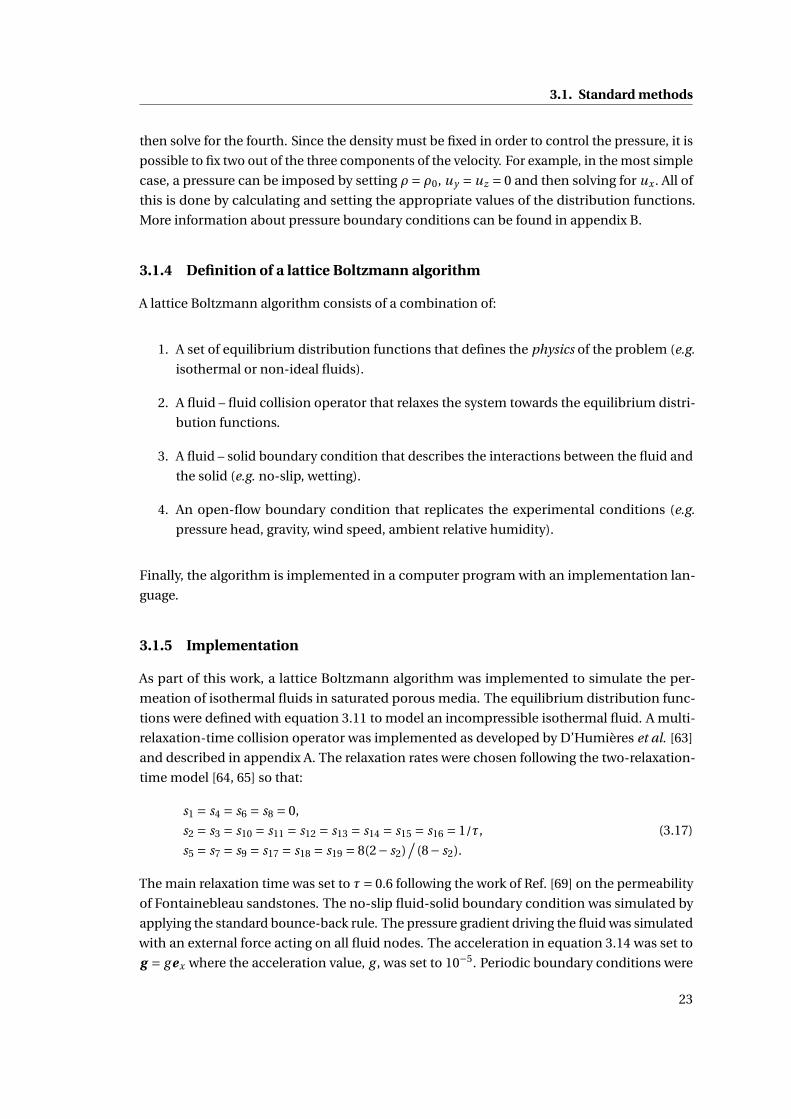
3.3 Permeability of a 3D square pipe . . . . . . . . . . . . . . . . . . . . . . . . . . . . 25
3.4 Illustration of an array of overlapping spheres . . . . . . . . . . . . . . . . . . . . 25
3.5 Permeability of an array of overlapping spheres with 20% porosity. . . . . . . . . 26
3.6 Permeability of an array of overlapping spheres of size L3 = 213. . . . . . . . . . 26
3.7 Effect of the viscosity on the permeability . . . . . . . . . . . . . . . . . . . . . . . 27
3.8 Illustration of the effective media model . . . . . . . . . . . . . . . . . . . . . . . 29
3.9 Illustration of the setup used for setting the pressure boundary conditions . . . 32
3.10 Permeability of a 3D square pipe . . . . . . . . . . . . . . . . . . . . . . . . . . . . 33
3.11 Permeability of a 3D square pipe: comparison of two algorithms. . . . . . . . . . 34
3.12 Permeability of an array of overlapping spheres with 20% porosity. . . . . . . . . 34
3.13 Permeability of an array of overlapping spheres: comparison of two algorithms. 35
3.14 Permeability of homogeneous media . . . . . . . . . . . . . . . . . . . . . . . . . 35
3.15 Permeability of homogeneous media: comparison with literature . . . . . . . . 36
3.16 Pressure drop across homogeneous media . . . . . . . . . . . . . . . . . . . . . . 36
3.17 Permeability of an array of permeable spheres . . . . . . . . . . . . . . . . . . . . 37
3.18 Clips of the velocity in an array of permeable spheres . . . . . . . . . . . . . . . . 38
3.19 Illustration of parallel and series layered media . . . . . . . . . . . . . . . . . . . 39
3.20 Illustration of a heterogenous medium . . . . . . . . . . . . . . . . . . . . . . . . 40
3.21 Pressure drop in a heterogeneous medium . . . . . . . . . . . . . . . . . . . . . . 40
3.22 Illustration of the simulation setup test case 3 . . . . . . . . . . . . . . . . . . . . 41
3.23 Velocity profile for test case 3 as reported in literature . . . . . . . . . . . . . . . 41
3.24 Velocity profile for test case 3 as calculated in this work . . . . . . . . . . . . . . 42
xv
List of Figures
4.1 Schematic illustration of the phase diagram P −V of a van der Waals fluid. . . . 45
4.2 Contact angleΘ vs. the surface-normal fluid density gradient. . . . . . . . . . . 48
4.3 Pressure drop across the liquid – vapour interface of a droplet . . . . . . . . . . 49
4.4 Capillary rise vs. the square root of time. . . . . . . . . . . . . . . . . . . . . . . . 49
4.5 Pendular rings formed between packed spheres. . . . . . . . . . . . . . . . . . . 50
4.6 Effect of the simulation temperature on the fluid distribution . . . . . . . . . . . 50
4.7 Fluid distribution for a liquid droplet in vapour . . . . . . . . . . . . . . . . . . . 52
4.8 Pressure drop across the liquid – vapour interface of a droplet. . . . . . . . . . . 52
4.9 Pressure drop across the liquid – vapour interface of a droplet: effect of the
interface width. . . . . . . . . . . . . . . . . . . . . . . . . . . . . . . . . . . . . . . 53
4.10 Spinodal decomposition . . . . . . . . . . . . . . . . . . . . . . . . . . . . . . . . . 53
4.11 Solid-bound spinodal decomposition . . . . . . . . . . . . . . . . . . . . . . . . . 54
4.12 Equilibrium contact angles on solid surfaces . . . . . . . . . . . . . . . . . . . . . 55
4.13 Illustration of a convex pore . . . . . . . . . . . . . . . . . . . . . . . . . . . . . . . 56
4.14 Kelvin’s equation . . . . . . . . . . . . . . . . . . . . . . . . . . . . . . . . . . . . . 56
4.15 Illustration of three serially connected pores . . . . . . . . . . . . . . . . . . . . . 57
4.16 Inkbottle effect: equilibrium fluid distribution during desorption . . . . . . . . 57
4.17 Inkbottle effect: non-equilibrium fluid distribution during desorption . . . . . 58
4.18 Inkbottle effect: equilibrium fluid distribution during adsorption . . . . . . . . 59
4.19 Inkbottle effect: non-equilibrium fluid distribution during adsorption . . . . . 59
4.20 Grey-bound spinodal decomposition . . . . . . . . . . . . . . . . . . . . . . . . . 62
4.21 Equilibrium contact angles on grey surfaces . . . . . . . . . . . . . . . . . . . . . 64
4.22 Isotherms of grey nodes: effect of internal wetting . . . . . . . . . . . . . . . . . . 64
4.23 Isotherms of grey nodes: effect of permeability and size . . . . . . . . . . . . . . 65
4.24 Pseudo-random systems . . . . . . . . . . . . . . . . . . . . . . . . . . . . . . . . . 66
4.25 Pseudo-random systems: water isotherms . . . . . . . . . . . . . . . . . . . . . . 66
4.26 Pseudo-random systems: water isotherms . . . . . . . . . . . . . . . . . . . . . . 67
4.27 Pseudo-random systems: water isotherms . . . . . . . . . . . . . . . . . . . . . . 67
4.28 Pseudo-random systems: equilibrium fluid distribution during desorption and
adsorption . . . . . . . . . . . . . . . . . . . . . . . . . . . . . . . . . . . . . . . . . 68
4.29 Pseudo-random systems: equilibrium fluid distribution during desorption and
adsorption . . . . . . . . . . . . . . . . . . . . . . . . . . . . . . . . . . . . . . . . . 68
5.1 Model cement paste microstructure generated with µic. . . . . . . . . . . . . . . 73
5.2 Solid and pore volumes in a µic model cement paste . . . . . . . . . . . . . . . . 73
5.3 Calculated permeability vs. the degree of hydration for different water-to-cement
ratios. . . . . . . . . . . . . . . . . . . . . . . . . . . . . . . . . . . . . . . . . . . . . 74
5.4 Calculated permeability vs. the porosity for different water-to-cement ratios. . 74
5.5 Illustration of lattice magnification . . . . . . . . . . . . . . . . . . . . . . . . . . 75
5.6 Illustration of microstructural resolution . . . . . . . . . . . . . . . . . . . . . . . 76
5.7 Illustration of diagonal leaks . . . . . . . . . . . . . . . . . . . . . . . . . . . . . . 77
5.8 Model cement paste microstructures generated with µic and CEMHYD3D. . . . 79
xvi
List of Figures
5.9 Partially-saturated model cement paste microstructures . . . . . . . . . . . . . . 82
5.10 Permeability vs. degree of capillary water saturation . . . . . . . . . . . . . . . . 83
5.11 Permeability vs. degree of capillary water saturation: effect of the C-S-H . . . . 84
6.1 Experimental water isotherms of cement paste. . . . . . . . . . . . . . . . . . . . 90
6.2 Model water isotherm of a µic model cement paste. . . . . . . . . . . . . . . . . . 91
6.3 Model water isotherm of a µic model cement paste: comparison of two methods 92
6.4 Model water isotherm of a µic model cement paste: effect of χ. . . . . . . . . . . 92
6.5 Model cement paste microstructure generated with µic . . . . . . . . . . . . . . 93
6.6 Model water isotherms of the capillary and gel pores of cement paste. . . . . . . 94
6.7 Model water isotherms of the capillary and gel pores of cement paste. . . . . . . 94
6.8 Effect of the internal wetting potential of the C-S-H on the model isotherms of
cement paste. . . . . . . . . . . . . . . . . . . . . . . . . . . . . . . . . . . . . . . . 95
6.9 Equilibrium fluid distribution during desorption in a µic microstructure . . . . 96
6.10 Equilibrium fluid distribution during adsorption in a µic microstructure . . . . 97
xvii

List of Tables2.1 Experimental measurements of permeability . . . . . . . . . . . . . . . . . . . . 9
3.1 Relative error in permeability for structures built from layers of different effective
media parameter. . . . . . . . . . . . . . . . . . . . . . . . . . . . . . . . . . . . . . 39
4.1 Simulated equilibrium contact angles between liquid and solid. . . . . . . . . . 55
4.2 Simulated equilibrium contact angles between liquid and grey nodes. . . . . . . 63
5.1 Densities of the reactants and hydrates used for the simulation of the cement
paste model microstructures. . . . . . . . . . . . . . . . . . . . . . . . . . . . . . . 72
5.2 Effect of the lattice magnification and microstructural resolution on the perme-
ability . . . . . . . . . . . . . . . . . . . . . . . . . . . . . . . . . . . . . . . . . . . . 77
5.3 Permeability to water and gas of the different cement paste phases. . . . . . . . 82
6.1 Effect of the simulation temperature on the emptying RH of a pore . . . . . . . 98
xix

Nomenclature
Abbreviation DescriptionPermeability Intrinsic permeability
w/c Water-to-cement ratio by mass
RH Relative humidity
NMR Nuclear magnetic resonance
C-S-H Calcium silicate hydrate
MIP Mercury intrusion porosimetry
ITZ Interfacial transition zone
REV Representative elementary volume
RHS Right-hand-side
LHS Left-hand-side
N.A. Not applicable
CFD Computational fluid dynamics
LB Lattice Boltzmann
BGK Bhatnagar-Gross-Krook
SRT Single-relaxation-time
TRT Two-relaxation-time
MRT Multi-relaxation-time
Lattice magnification See figure 5.5
Microstructural resolution Minimum feature size, see figure 5.6
Symbol DescriptionA Cross section of a sample of length L0
L0 Length of a sample of cross section A
L Side length of a cubic sample
(Lx ,Ly ,Lz ) Dimensions of a sample
r = (lx , ly , lz ) Coordinates of a lattice node
h Width and height of an infinitely long sample
r Radius of a sphere or circle
Q Number of directions in the lattice Boltzmann method
ei Velocity vectors
wi Lattice weights
xxi

Nomenclature
∆x Lattice spacing
∆t Time step
∆ρ Density unit
c Speed unit (∆x/∆t )
cs Speed of sound
fi Distribution functions
f eqi Equilibrium distribution functions
F External force
g Body-force
S Diagonal relaxation matrix
si Relaxation times of the diagonal relaxation matrix S
τ Main relaxation time
M Transformation matrix
m Hydraulic moments
ρ Macroscopic density
ρ∗ Microscopic density
ρ0 Average density in the system
u Macroscopic velocity
u∗ Microscopic velocity
j Macroscopic moment
δi j Kronecker delta
N xy , N x
z Transverse momentum corrections for the pressure boundary conditions
J Fluid flow
µ Dynamics viscosity
υ Kinematic viscosity
∆P Pressure drop
κ Intrinsic permeability
β Brinkman’s effective viscosity
ε Fractional error
CD Drag force coefficient
σ Effective media parameter
ns Solid fraction (equivalent to the effective media parameter σ)
γ Surface tension
M∗ Molar mass
R Universal gas constant
T Temperature
Tc Critical temperature
V Volume
P Pressure
Pα,β Pressure tensor
ξ Pressure scaling factor
p0 Bulk pressure
xxii

Nomenclature
θ Reduced temperature
θc Reduced critical temperature
χ Parameter related to the surface tension
ρc Reduced critical density
ρl i qui d Reduced liquid density
ρg as Reduced gas density
$ Width of the liquid - vapour interface
λ Parameter related to the Galilean invariance
ωp,t ,αα,αβ Adjustable constants
Ψ Free energy functional
ψ Free energy density
Φ Surface free energy density
φ Wetting potential between fluid and solid
Ω Dimension-less wetting potential between fluid and solid
Θ Contact angle between liquid fluid and solid
φα,β Wetting potential between α and β
Θα,β Contact angle between liquid in α and surface of β
φg r e y Internal wetting potential of grey nodes
Sς Surface ς
Vg r e y Volume of grey nodes
xxiii

1 Introduction
Contents
1.1 Concrete . . . . . . . . . . . . . . . . . . . . . . . . . . . . . . . . . . . . . . . . 1
1.2 From concrete to cement paste . . . . . . . . . . . . . . . . . . . . . . . . . . . 1
1.3 Indicators of durability . . . . . . . . . . . . . . . . . . . . . . . . . . . . . . . 3
1.4 Statement of the problem . . . . . . . . . . . . . . . . . . . . . . . . . . . . . . 4
1.1 Concrete
Concrete is the most widely used material on Earth. The current yearly production exceeds
1010 m3 and is enough to build a 5 m2 beam that stretches from Earth to the Moon∗. This
huge ever-increasing volume means that, although concrete is a material with intrinsically
low CO2 emissions, it is responsible for some 5 to 8% of global man-made emissions [1].
Consequently, it is of great environmental interest to design new concretes with lower CO2
footprints. Nonetheless, the challenge is that they must have comparable or improved, and
predictable properties, notably in terms of resistance to degradation and durability.
Water transport underpins most physical and chemical degradation mechanisms. Water is
transported through porous materials by advection, diffusion, and absorption. In concrete
structures, the transport of water strongly impacts durability both directly, e.g. freeze-thaw
action, and indirectly by permitting the ingress of aggressive ions.
1.2 From concrete to cement paste
Concrete is made by mixing aggregates, cement and water. The water reacts with cement
to form cement paste, the glue that binds the aggregates together to form a rock-solid mass.
Concrete is often regarded as a composite material composed of aggregates, cement paste
∗Unfortunately, gravity prevents us from doing so.
1
Chapter 1. Introduction
and an interfacial transition zone (ITZ) between them. The ITZ is the region of the paste that
surrounds the aggregates and is perturbed their presence. This perturbation leads to a local
increase in porosity [2]. The properties of concrete are dependent on the individual properties
of its components but are mainly determined by the quality of the cement paste. Therefore,
the introduction of any new concrete must be preceded by a quantitative understanding of
the microstructure, properties and durability of cement paste.
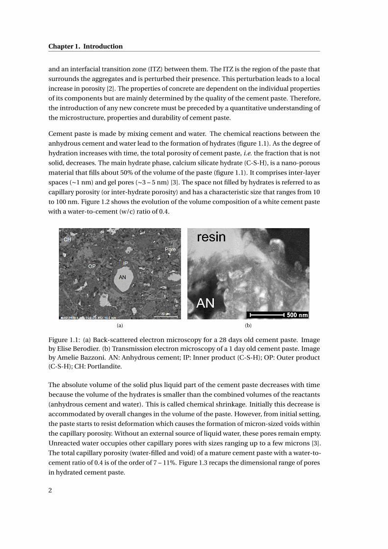
Cement paste is made by mixing cement and water. The chemical reactions between the
anhydrous cement and water lead to the formation of hydrates (figure 1.1). As the degree of
hydration increases with time, the total porosity of cement paste, i.e. the fraction that is not
solid, decreases. The main hydrate phase, calcium silicate hydrate (C-S-H), is a nano-porous
material that fills about 50% of the volume of the paste (figure 1.1). It comprises inter-layer
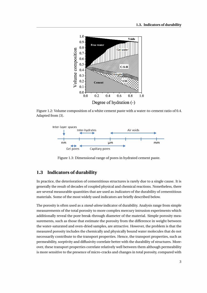
spaces (∼1 nm) and gel pores (∼3 – 5 nm) [3]. The space not filled by hydrates is referred to as
capillary porosity (or inter-hydrate porosity) and has a characteristic size that ranges from 10
to 100 nm. Figure 1.2 shows the evolution of the volume composition of a white cement paste
with a water-to-cement (w/c) ratio of 0.4.
(a) (b)
Figure 1.1: (a) Back-scattered electron microscopy for a 28 days old cement paste. Imageby Elise Berodier. (b) Transmission electron microscopy of a 1 day old cement paste. Imageby Amelie Bazzoni. AN: Anhydrous cement; IP: Inner product (C-S-H); OP: Outer product(C-S-H); CH: Portlandite.
The absolute volume of the solid plus liquid part of the cement paste decreases with time
because the volume of the hydrates is smaller than the combined volumes of the reactants
(anhydrous cement and water). This is called chemical shrinkage. Initially this decrease is
accommodated by overall changes in the volume of the paste. However, from initial setting,
the paste starts to resist deformation which causes the formation of micron-sized voids within
the capillary porosity. Without an external source of liquid water, these pores remain empty.
Unreacted water occupies other capillary pores with sizes ranging up to a few microns [3].
The total capillary porosity (water-filled and void) of a mature cement paste with a water-to-
cement ratio of 0.4 is of the order of 7 – 11%. Figure 1.3 recaps the dimensional range of pores
in hydrated cement paste.
2
1.3. Indicators of durability
Figure 1.2: Volume composition of a white cement paste with a water-to-cement ratio of 0.4.Adapted from [3].
Figure 1.3: Dimensional range of pores in hydrated cement paste.
1.3 Indicators of durability
In practice, the deterioration of cementitious structures is rarely due to a single cause. It is
generally the result of decades of coupled physical and chemical reactions. Nonetheless, there
are several measurable quantities that are used as indicators of the durability of cementitious
materials. Some of the most widely used indicators are briefly described below.
The porosity is often used as a stand-alone indicator of durability. Analysis range from simple
measurements of the total porosity to more complex mercury intrusion experiments which
additionally reveal the pore break-through diameter of the material. Simple porosity mea-
surements, such as those that estimate the porosity from the difference in weight between
the water-saturated and oven-dried samples, are attractive. However, the problem is that the
measured porosity includes the chemically and physically bound water molecules that do not
necessarily contribute to the transport properties. Hence, the transport properties, such as
permeability, sorptivity and diffusivity correlate better with the durability of structures. More-
over, these transport properties correlate relatively well between them although permeability
is more sensitive to the presence of micro-cracks and changes in total porosity, compared with
3
Chapter 1. Introduction
diffusivity or sorptivity [4].
The intrinsic permeability characterizes a medium from the perspective of pressure-induced
fluid flow through the fully saturated porosity. It quantifies the ability of a material to resist
fluid penetration and consequently correlates well with durability. It is related to macroscopic
observables through Darcy’s law [5]. For cement paste with water-to-cement ratios ≤ 0.5, it is
very low and difficult to measure reliably. Hence, there is a paucity of experimental data and a
considerable variability.
With the exception of the near-surface, concrete structures are rarely saturated with water. In
partially-saturated materials, suction leads the the uptake of water. This is called absorption
and can be described by the extended Darcy equation. Moreover, the partially saturated struc-
tures can be exposed to variations in the ambient relative humidity (RH). These changes lead
to the egress (desorption) and ingress (adsorption) of liquid water and vapour. The adsorp-
tion and desorption isotherms, also known as the water isotherms, describe the equilibrated
systems below full saturation and quantify the liquid - vapour - solid interactions.
The diffusion of water vapour and ions affect the durability of cementitious structures. In
practice, ions, such as chloride and sulfates, diffuse in the liquid-saturated part of the struc-
tures. The former causes extensive cracking and the latter leads to the corrosion of the steel
rebars. Other degradation mechanisms that are based on diffusion include carbonation where
the CO2 diffuses through the empty porosity and reacts with the portlandite. Although the
mechanisms that govern the water vapour and gas diffusion are dissimilar, the latter is often
used as a durability indicator because it is easier to measure.
1.4 Statement of the problem
The measurement of transport properties is necessary to control the quality and predict the
durability of cement paste. However, the experiments are often time-consuming and in some
cases, e.g. permeation of water, show a large unexplained scatter and anomalous behaviour
(see chapter 2).
Computer models can help address these problems. More importantly, they can help to
understand the link between the microstructure and the performance of the material. They
also make it possible to isolate the effects of various parameters which is very difficult to do
in experiments. These advantages are critical en route to develop better, more predictable
materials.
Computational fluid dynamics models have been successfully used to understand water
transport in a wide range of porous media including sandstones [6], carbonates [7] and fuel
cells [8]. However, their application to cement paste remains rather limited [9, 10, 11, 12, 13].
Numerical models have been restricted to either molecular dynamics simulations at the nano-
scale [14, 15] or to rather simplified models of flow through the micron-sized capillary pores
4
1.4. Statement of the problem
[9, 16, 17, 18, 10, 11, 12]. The general consensus is that the macroscopic properties of cement
paste are governed by transport through the capillary pores. However, the models which are
limited to the capillary pores fail to reproduce experimental measurements [9, 16, 18, 10, 11,
12]. Moreover, in aggressive environments where structures are exposed to sea-water, high
performance concretes are often used. The cement pastes of these concretes have a smaller
and finer porosity and the measurement of their transport properties is consequently more
laborious and more time-consuming. These factors make it crucial to develop novel models
that can predict the water dynamics and interactions in both capillary and C-S-H gel pores.
The objective of this thesis is to develop a numerical model that calculates the permeability of
cement paste based on its microstructure. The layout of the thesis is as follows.
Chapter 2 reviews the experimental and numerical methods that are used to measure and
model the permeability of cement paste. Emphasis is put on the large scatter in experimental
data and on the limitations of the current numerical models.
Chapter 3 presents two lattice Boltzmann models for isothermal fluids. The first method is a
relatively standard flow model that is limited to the capillary pores. The second additionally
accounts for the flow through the C-S-H gel pores via an effective media approach. These two
methods are used to simulate the permeability of model cement pastes in chapter 5 where
it is shown that the degree of water saturation and the flow through the C-S-H are critical to
correctly match the experimental permeability measurements.
In chapter 4, the lattice Boltzmann permeability model is extended to non-ideal fluids de-
scribed with an equation of state. This modification is necessary to model the desorption
and adsorption of liquid water and vapour in the capillary pores. The model is further ex-
tended to include the transport and isotherms in the C-S-H gel pores. This is achieved with a
novel effective media approach implemented within a free energy framework. The method is
demonstrated in section 4.2.6 on pseudo-random cement-like systems. It is shown that the
novel LB model can reproduce a two-step isotherm where the first corresponds to the capillary
pores and the second to the smaller gel pores. It is also shown that the model can reproduce
the ink-bottle effect. The model is used to simulate the desorption and adsorption in model
cement pastes in chapter 6 where it is shown that it is critical to take into account the C-S-H
gel pores in order to match the experimental water isotherms.
Finally, chapter 7 summarizes the insights discovered during this thesis and provides an
outlook for possible future work.
5

2 Permeability of Cement Paste: State-of-the-art
Contents
2.1 Darcy’s law . . . . . . . . . . . . . . . . . . . . . . . . . . . . . . . . . . . . . . . 7
2.2 Experimental techniques . . . . . . . . . . . . . . . . . . . . . . . . . . . . . . 8
2.3 Modelling techniques . . . . . . . . . . . . . . . . . . . . . . . . . . . . . . . . 10
2.3.1 Empirical models . . . . . . . . . . . . . . . . . . . . . . . . . . . . . . . . 10
2.3.2 Numerical models . . . . . . . . . . . . . . . . . . . . . . . . . . . . . . . 11
2.4 Experiments and models: a mismatch ? . . . . . . . . . . . . . . . . . . . . . . 15
This chapter reviews the techniques that are used to calculate the permeability of cement paste.
First, section 2.1 introduces Darcy’s law. Then, sections 2.2 and 2.3 discuss the experimental
and numerical techniques that are used to measure and model permeability, respectively.
Finally, section 2.4 discusses the reasons behind the mismatch between the experiments and
models.
2.1 Darcy’s law
The intrinsic∗ permeability κ characterizes a medium from the perspective of pressure-
induced fluid flow through the fully saturated porosity. For incompressible liquids and viscous
flows, it is related to macroscopic observables through Darcy’s law [5] which may be written
under the form:
κ= L0
A
µJ
∆P(2.1)
for a sample of length L0 and cross-sectional area A through which a fluid flow J is driven by
an applied pressure gradient ∆P (figure 2.1). The dynamic fluid viscosity is µ= ρυ where ρ is
∗The non-intrinsic permeability, also called hydraulic conductivity, is fluid dependent and is expressed in m.s−1.The ratio of intrinsic permeability to hydraulic conductivity is given by µ/ρg where g is the acceleration due togravity. For water at 20, µ/ρg ' 10−7 m.s.
7
Chapter 2. Permeability of Cement Paste: State-of-the-art
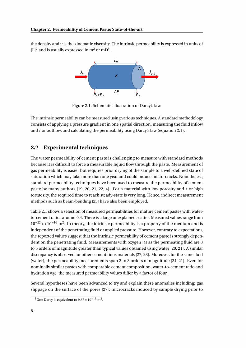
the density and υ is the kinematic viscosity. The intrinsic permeability is expressed in units of
[L]2 and is usually expressed in m2 or mD†.
Figure 2.1: Schematic illustration of Darcy’s law.
The intrinsic permeability can be measured using various techniques. A standard methodology
consists of applying a pressure gradient in one spatial direction, measuring the fluid inflow
and / or outflow, and calculating the permeability using Darcy’s law (equation 2.1).
2.2 Experimental techniques
The water permeability of cement paste is challenging to measure with standard methods
because it is difficult to force a measurable liquid flow through the paste. Measurement of
gas permeability is easier but requires prior drying of the sample to a well-defined state of
saturation which may take more than one year and could induce micro-cracks. Nonetheless,
standard permeability techniques have been used to measure the permeability of cement
paste by many authors [19, 20, 21, 22, 4]. For a material with low porosity and / or high
tortuosity, the required time to reach steady-state is very long. Hence, indirect measurement
methods such as beam-bending [23] have also been employed.
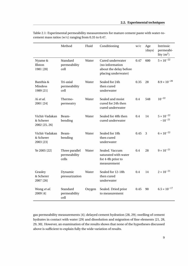
Table 2.1 shows a selection of measured permeabilities for mature cement pastes with water-
to-cement ratios around 0.4. There is a large unexplained scatter. Measured values range from
10−22 to 10−16 m2. In theory, the intrinsic permeability is a property of the medium and is
independent of the penetrating fluid or applied pressure. However, contrary to expectations,
the reported values suggest that the intrinsic permeability of cement paste is strongly depen-
dent on the penetrating fluid. Measurements with oxygen [4] as the permeating fluid are 3
to 5 orders of magnitude greater than typical values obtained using water [20, 21]. A similar
discrepancy is observed for other cementitious materials [27, 28]. Moreover, for the same fluid
(water), the permeability measurements span 2 to 3 orders of magnitude [24, 21]. Even for
nominally similar pastes with comparable cement composition, water-to-cement ratio and
hydration age, the measured permeability values differ by a factor of four.
Several hypotheses have been advanced to try and explain these anomalies including: gas
slippage on the surface of the pores [27]; microcracks induced by sample drying prior to
†One Darcy is equivalent to 9.87×10⁻¹³ m2.
8
2.2. Experimental techniques
Table 2.1: Experimental permeability measurements for mature cement paste with water-to-cement mass ratios (w/c) ranging from 0.35 to 0.47.
Method Fluid Conditioning w/c Age Intrinsic(days) permeabi-
lity (m2)
Nyame & Standard Water Cured underwater 0.47 600 5×10⁻²²
Illston permeability (no information1981 [20] cell about the delay before
placing underwater)
Banthia & Tri-axial Water Sealed for 24h 0.35 28 8.9×10⁻²⁰
Mindess permeability then cured1989 [21] cell underwater
Ai et al. Thermo- Water Sealed and moist 0.4 548 10−22
2001 [24] permeatry cured for 24h thencured underwater
Vichit-Vadakan Beam- Water Sealed for 48h then 0.4 14 5×10⁻²²
& Scherer bending cured underwater −10−21
2002 [25, 26]
Vichit-Vadakan Beam- Water Sealed for 18h 0.45 3 6×10⁻²²
& Scherer bending then cured2003 [23] underwater
Ye 2005 [22] Three parallel Water Sealed. Vaccum 0.4 28 9×10⁻²¹
permeability saturated with watercells for 4-8h prior to
measurement
Grasley Dynamic Water Sealed for 12-18h 0.4 14 2×10⁻²¹
& Scherer pressurization then cured2007 [26] underwater
Wong et al. Standard Oxygen Sealed. Dried prior 0.45 90 6.5×10⁻¹⁷
2009 [4] permeability to measurementcell
gas permeability measurements [4]; delayed cement hydration [28, 29]; swelling of cement
hydrates in contact with water [29] and dissolution and migration of fine elements [21, 28,
29, 30]. However, an examination of the results shows that none of the hypotheses discussed
above is sufficient to explain fully the wide variation of results.
9
Chapter 2. Permeability of Cement Paste: State-of-the-art
A plausible hypothesis is the variation in the degree of water saturation, defined as the fraction
of the porosity that is filled with water. Abbas et al. [31], Baroghel-Bouny et al. [32] and Wong
et al. [33] showed a strong dependency of the intrinsic gas permeability on the degree of water
saturation for concretes, mortars and other cement-based materials. At the start of this work,
the author was not aware of any similar study on cement paste using water as the permeating
fluid. Only very recently, Zamani et al. [34] measured the water permeability of cement paste as
a function of the internal relative humidity (RH) using a combination of 1H nuclear magnetic
resonance (NMR) analysis and empirical modelling. In general, although experimentalists
try to ensure water saturation before measuring water permeability, total saturation might
be difficult to establish and maintain. The analysis of the procedures leading to the results
reported in table 2.1 suggests that none of the measurements of water permeability to date
has actually been carried out on a fully saturated material.
The differences in water saturation of the capillary porosity primarily originate from the
conditioning of the samples after mixing. In systems which are cured sealed, the chemical
shrinkage voids are necessarily devoid of liquid water. In underwater cured systems, it is
often assumed that water is drawn into the voids as they form. However, this depends on
the size of the paste and the delay in exposing it to additional water. Water cannot permeate
across more than millimetre-sized samples on the timescale of the curing due to the rapidly
decreasing permeability of the paste and the relatively small pressure head. Hence for large
samples, such as might be used for permeability tests, and / or for water exposure delays of
more than a few hours, a significant fraction of the chemical shrinkage porosity may remain
devoid of liquid water. This is confirmed by recent 1H NMR experiments, which have also
shown that it is difficult, if not impossible, to subsequently saturate the shrinkage voids even
when using vacuum saturation on small samples [35]. This argument will be further developed
in sections 5.2.2 and 5.2.5 of chapter 5.
2.3 Modelling techniques
Models of water transport can be divided into two main categories. In the first category, simple
experimental measurements are combined with empirical equations in order to predict the
transport properties. In the second category, the flow is simulated through the explicitly
resolved porosity by solving or approximating the equations of flow. In this case, the pore
structure can be obtained by imaging techniques or simulated with a microstructural model.
2.3.1 Empirical models
Empirical equations can be combined with experimental measurements such as mercury
intrusion porosimetry (MIP) and electrical conductivity to calculate the water permeability.
For example, Katz and Thompson [36] proposed an empirical relation that describes the
permeability of rocks saturated with a single liquid phase with κ = cl 2cσσc
. Here, lc is the
characteristic pore size, σ is the conductivity of the rock saturated with a brine solution
10
2.3. Modelling techniques
of conductivity σ0, and c is a constant on the order of 1/226. They reported an excellent
relationship between the calculated and measured permeabilities for various sandstones [36,
37]. El-Dieb and Hooton [38] and Christensen et al. [39] used the Katz and Thompson model
to calculate the permeability of cement paste. They both reported a poor linear relationship
between the measured and calculated permeabilities. There are several reasons that can
explain the discrepancy. First, the Katz and Thompson equation was developed for fully
saturated rocks. As discussed in section 2.2, it appears that the cement paste samples that
are used for permeability experiments may not be fully saturated. Second, the Katz and
Thompson equation was tested on various sandstones. These rocks have a relatively coarse
porosity. Cement paste has a finer porosity and a wider pore size distribution with multiple
characteristic pore sizes (mainly capillary and gel pores). Third, it is unclear how pore sizes
determined with MIP on dried samples can be used to estimate the permeability of virgin
samples [38, 40].
Along these lines, Cui and Cahyadi [41] included the contribution of the C-S-H gel pores in the
permeability calculation by using an analytical expression derived from the general effective
media theory [42] for the calculation of the conductivity of bi-composite materials. The pore
structure characteristics were determined by MIP and the volume of hydrates with Power’s
model. They reported permeability coefficients in good agreement with measurements for
different w/c ratios and degrees of hydration. However, the model requires input quantities
that are practically impossible to measure such as the critical volume fraction of C-S-H.
Moreover, similarly to the application of the Katz and Thompson model to cement paste, it is
unclear how pore sizes determined with MIP on dried samples can be used to estimate the
permeability of virgin samples [38, 40].
2.3.2 Numerical models
Pore structure of cement paste
Imaging techniques The pore structure of cement paste can be reconstructed using micro-
tomographic images obtained with, for example, scanning electron microscopes or focused
ion beam. Although the obtained structures are realistic, there are several limitations. For
instance, the resolution is often limited to ∼ 0.1−1 µm which means that the inter-hydrates
and fine capillary pores cannot be resolved. Additionally, the resolution is larger than the
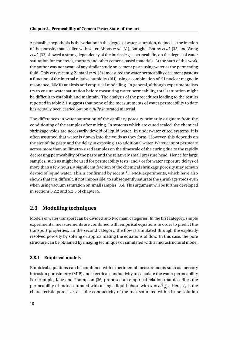
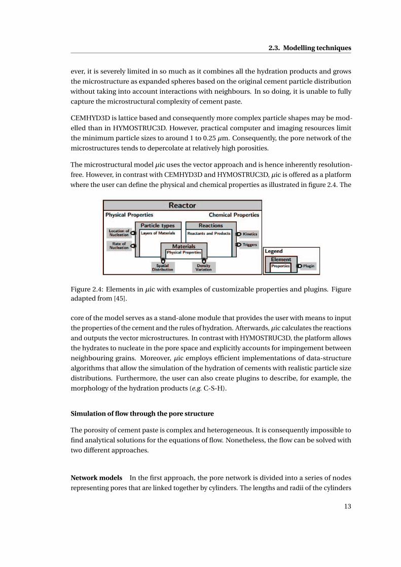
break through diameter obtained from mercury intrusion experiments. For example, figure 2.2
shows the pore size distribution for a 28 days old cement paste with a water-to-cement ratio
of 0.4 as obtained from a mercury intrusion experiment. The pore break-through radius is of
the order of 7 - 20 nm. This is smaller than the minimum feature that can be resolved with
traditional imaging techniques. Moreover, most imaging techniques require drying of the
sample which might damage the microstructure.
11
Chapter 2. Permeability of Cement Paste: State-of-the-art
Figure 2.2: Pore size distribution of a 28 days old cement paste with a w/c ratio of 0.4 asobtained with mercury intrusion porosimetry. Data from Elise Berodier.
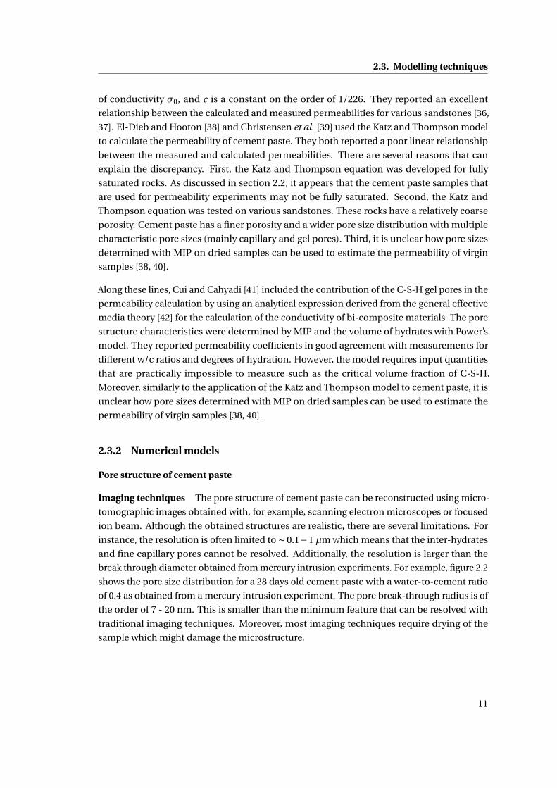
Microstructural models Microstructural models of cement paste have been developed
for the purpose of understanding cement hydration and kinetics. Some of these models
account for a range of properties derived from the chemistry and thermodynamics of cement
such as phase composition, assemblage and interactions during the hydration processes.
HYMOSTRUC3D [43], CEMHYD3D [44] and µic [45] are amongst the leading models.
(a) (b)
Figure 2.3: 2D images of cement model microstructures as obtained with (a) µic and (b)CEMHYD3D. The microstructures are (100 µm)3 in size. In (a) The model is of a white cementpaste with a w/c ratio of 0.4 and after 17 hours of hydration. The main phases are alite (red),monosulfate (purple), ettringite (pale green), aluminate (white), C-S-H (cyan), portlandite(green) and pores (black). In (a), (b) the model is of a CEM I cement paste with a w/c ratioof 0.5 and after 28 days of hydration. The main phases are: alite (light brown), belite (blue),aluminate (grey), aluminoferrrite (white), C-S-H (beige), portlandite (dark blue) and pores(black).
HYMOSTRUC3D uses the vector approach to generate resolution-free microstructures. How-
12
2.3. Modelling techniques
ever, it is severely limited in so much as it combines all the hydration products and grows
the microstructure as expanded spheres based on the original cement particle distribution
without taking into account interactions with neighbours. In so doing, it is unable to fully
capture the microstructural complexity of cement paste.
CEMHYD3D is lattice based and consequently more complex particle shapes may be mod-
elled than in HYMOSTRUC3D. However, practical computer and imaging resources limit
the minimum particle sizes to around 1 to 0.25 µm. Consequently, the pore network of the
microstructures tends to depercolate at relatively high porosities.
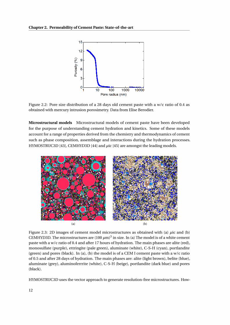
The microstructural model µic uses the vector approach and is hence inherently resolution-
free. However, in contrast with CEMHYD3D and HYMOSTRUC3D, µic is offered as a platform
where the user can define the physical and chemical properties as illustrated in figure 2.4. The
Figure 2.4: Elements in µic with examples of customizable properties and plugins. Figureadapted from [45].
core of the model serves as a stand-alone module that provides the user with means to input
the properties of the cement and the rules of hydration. Afterwards,µic calculates the reactions
and outputs the vector microstructures. In contrast with HYMOSTRUC3D, the platform allows
the hydrates to nucleate in the pore space and explicitly accounts for impingement between
neighbouring grains. Moreover, µic employs efficient implementations of data-structure
algorithms that allow the simulation of the hydration of cements with realistic particle size
distributions. Furthermore, the user can also create plugins to describe, for example, the
morphology of the hydration products (e.g. C-S-H).
Simulation of flow through the pore structure
The porosity of cement paste is complex and heterogeneous. It is consequently impossible to
find analytical solutions for the equations of flow. Nonetheless, the flow can be solved with
two different approaches.
Network models In the first approach, the pore network is divided into a series of nodes
representing pores that are linked together by cylinders. The lengths and radii of the cylinders
13
Chapter 2. Permeability of Cement Paste: State-of-the-art
are determined by the pore separation and throat size. Then, the equations of laminar flow
within this network of cylinders, essentially a large set of simultaneous equations, are solved.
Most previous attempts to simulate the water permeability of cement paste are based on
such network models [16, 18, 17]. Pignat et al. [16] reported intrinsic permeability values
of the order of 10−13 to 10−15 m2 depending on the porosity and the cement particle size
distribution using the microstructural model IKPM, a precursor of µic, for a w/c ratio of 0.42.
Using microstructures simulated with HYMOSTRUC3D, Ye et al. [18] reported permeabilities
varying from 10−16 to 10−20 m2 depending on the porosity for a paste with a w/c ratio of 0.4.
Related to these studies, Koster et al. [17] derived a network model from 1 µm resolution 3D
micro-tomographic images of cement pastes and calculated a single permeability value of
9.3×10⁻²⁰ m2 for a sample with a w/c ratio of 0.45 and a degree of hydration of 0.67.
The large difference in the values reported by Pignat et al. [16] and Ye et al. [18] is rather
surprising since they both approximate the flow using network models in microstructures
essentially composed of overlapping spheres. At similar porosities, ∼ 20%, Pignat et al. report
a permeability of ∼ 3×10⁻¹⁵ m2 while Ye et al. report a permeability of ∼ 10−19 m2. This
difference outlines the degrees of freedom that are available in network models due to the
different possible means to choose the number, radius and connectivity of the nodes.
Discrete models To avoid inadvertent change of the pore structure, the second approach
consists of solving - not approximating - the equations of flow using numerical methods such
as finite element or lattice Boltzmann. This approach removes the requirement to reduce the
highly complex pore structure into a series of cylinders and was previously used by Garboczi
and Bentz [9] and Zhang et al. [12].
Garboczi and Bentz [9] used a lattice Boltzmann model to calculate the permeability of
CEMHYD3D cement paste microstructures as a function of the capillary porosity and mi-
crostructure resolution (minimum particle size). They reported that the calculated perme-
ability was very sensitive to the resolution of the microstructure and at the highest resolution
studied (0.25 µm), the permeability was circa 10−17 m2 at a capillary porosity of 12%. Most
recently, Zhang et al. [12] used the LB method to calculate the permeability of HYMOSTRUC3D
cement paste microstructures. They reported a permeability of approximately 2×10⁻¹⁸ m2
for a w/c ratio of 0.4, a hydration age of 50 days and a microstructure resolution of 0.5 µm.
In general, the water permeabilities obtained with discrete numerical models are of the
order 10−17 −10−18 m2, several orders of magnitude larger than the lowest water permeability
measurement and closer to the gas result (table 2.1).
14
2.4. Experiments and models: a mismatch ?
2.4 Experiments and models: a mismatch ?
The measured permeabilities show a considerable scatter. For mature cement pastes with
w/c ratios around 0.4, the permeabilities range from 10−22 to 10−16 m2 (table 2.1). For reasons
outlined in section 2.2, it appears that most measurements have been done on non-saturated
samples. In this case, the measurements are no longer of intrinsic permeability.
The values obtained using computer models are scattered as well and range from 10−20 to 10−15
m2. Here, there are several problems that need to be addressed. First, previous simulations
only addressed fully saturated porosity. Hence, they cannot be compared to the reported
experiments without matching the conditioning of the samples in the experiments with the
degree of water saturation in the models. Second, at high degrees of hydration and low degrees
of water saturation, the water-filled capillary porosity depercolates and the nano-porosity
of the C-S-H becomes crucial to maintain the percolation of the water-filled pore network.
Previous simulations only addressed the capillary porosity and ignored the nano-scale porosity.
With the exception of the analytical work of Cui and Cahyadi [41], all the simulations discussed
above treated the C-S-H phase as an impermeable solid with no inherent porosity. This makes
the percolation of the pore network, and thus the permeability, critically dependent on the
resolution of the microstructures. These factors lead to an overestimation of the permeability
at large porosity and cause it to fall catastrophically to zero below the percolation threshold of
the capillary porosity.
Consequently, what is required to clear up the mismatch is a numerical model that can
account for the degree of water saturation and solve the flow in both the capillary and gel
pores. Discrete methods, such as finite element and lattice Boltzmann, can do so. Additionally,
they offer the advantage of solving the flow without the need to reduce the pore structure
into a series of cylinders. Furthermore, they can help develop more pathways for testing the
microstructural models of cement paste against experimental data.
In this context, the lattice Boltzmann method was selected for solving the equations of flow. It
was previously used by Garobczi and Bentz [9] to calculate the permeability of cement paste
and by Svec et al. [46] to study the flow of fibre reinforced self-compacting concrete during a
slump test. Besides the advantages discussed in the last paragraph, it offers the ability to deal
implicitly with arbitrarily shaped geometries which is critical for complex porous media like
cement paste. Moreover, the computer code that would be initially developed for permeability
could be extended to model a wide range of transport phenomena including diffusion and
desorption. In the latter case, lattice Boltzmann methods give a significant advantage over
other discrete methods because they offer an implicit tracking of the liquid - vapour interfaces.
15

3 Lattice Boltzmann Methods forIsothermal Fluids
Contents
3.1 Standard methods . . . . . . . . . . . . . . . . . . . . . . . . . . . . . . . . . . 17
3.1.1 Overview . . . . . . . . . . . . . . . . . . . . . . . . . . . . . . . . . . . . . 17
3.1.2 Collision operators and equilibrium functions . . . . . . . . . . . . . . . 20
3.1.3 Boundary conditions . . . . . . . . . . . . . . . . . . . . . . . . . . . . . . 21
3.1.4 Definition of a lattice Boltzmann algorithm . . . . . . . . . . . . . . . . 23
3.1.5 Implementation . . . . . . . . . . . . . . . . . . . . . . . . . . . . . . . . . 23
3.1.6 Methods for calculating permeability . . . . . . . . . . . . . . . . . . . . 24
3.1.7 Validation . . . . . . . . . . . . . . . . . . . . . . . . . . . . . . . . . . . . 24
3.2 Effective media methods for the transport properties . . . . . . . . . . . . . 27
3.2.1 Overview . . . . . . . . . . . . . . . . . . . . . . . . . . . . . . . . . . . . . 27
3.2.2 Theory . . . . . . . . . . . . . . . . . . . . . . . . . . . . . . . . . . . . . . 29
3.2.3 Implementation . . . . . . . . . . . . . . . . . . . . . . . . . . . . . . . . . 31
3.2.4 Methods for calculating permeability . . . . . . . . . . . . . . . . . . . . 32
3.2.5 Validation . . . . . . . . . . . . . . . . . . . . . . . . . . . . . . . . . . . . 32
3.1 Standard methods
3.1.1 Overview
Over the past 25 years, a new class of computational fluid dynamics solver, the lattice Boltz-
mann (LB) method, has emerged [47, 48, 49, 50, 51, 52, 53, 54]. A large amount of research
effort has resulted in a large inventory of lattice Boltzmann algorithms suitable for a wide
range of applications including the simulation of multi-component [55] and multi-phase
non-ideal fluids [56], chemical reactions [7], turbulence [57], magneto hydrodynamics [58],
relativistic hydrodynamics [59], heat transfer [60] and free surface flows [61]. The successful
development of LB methods is due to several factors. First, in its most basic form, an LB
17
Chapter 3. Lattice Boltzmann Methods for Isothermal Fluids
algorithm is easier to implement than other computational fluid dynamics solvers based on
the direct discretization of the Navier-Stokes equations. Second, the LB methods are based on
a mesoscopic description of fictitious fluid particles. This makes it easy to incorporate several
types of interactions between the fluid particles, and to describe interactions between the
fluid and solid boundaries. This includes the ability to describe complex boundaries by means
of very simple arithmetical operations. Moreover, due to the local nature of the interactions,
most LB algorithms are highly amenable to parallelization and can take advantage of the
recent growth in computing power.
Historically, the lattice Boltzmann approach developed from the lattice gas method [48, 49]
but it can also be directly derived from the Boltzmann equation [62] which describes the
statistical behaviour of a system that is not in thermodynamic equilibrium. Under appropriate
conditions, the LB equations are formally equivalent to the Navier-Stokes equations discretized
in space and time [51]. The Navier-Stokes equations emerge from applying the second law
of Newton to fluid motion and assuming that the stress in the fluid is the sum of a pressure
term and a diffusing viscous term. They are of paramount importance in physics as they
successfully describe, amongst other things, water flows, oceans currents and air turbulence.
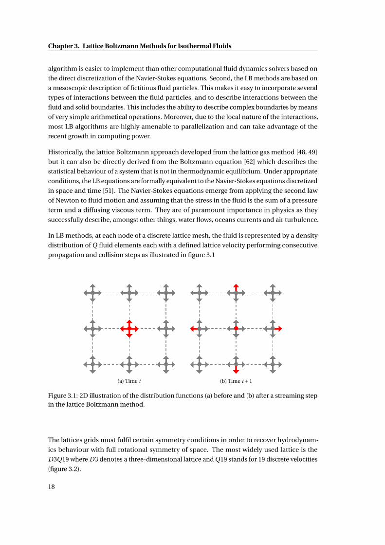
In LB methods, at each node of a discrete lattice mesh, the fluid is represented by a density
distribution of Q fluid elements each with a defined lattice velocity performing consecutive
propagation and collision steps as illustrated in figure 3.1
(a) Time t (b) Time t +1
Figure 3.1: 2D illustration of the distribution functions (a) before and (b) after a streaming stepin the lattice Boltzmann method.
The lattices grids must fulfil certain symmetry conditions in order to recover hydrodynam-
ics behaviour with full rotational symmetry of space. The most widely used lattice is the
D3Q19 where D3 denotes a three-dimensional lattice and Q19 stands for 19 discrete velocities
(figure 3.2).
18
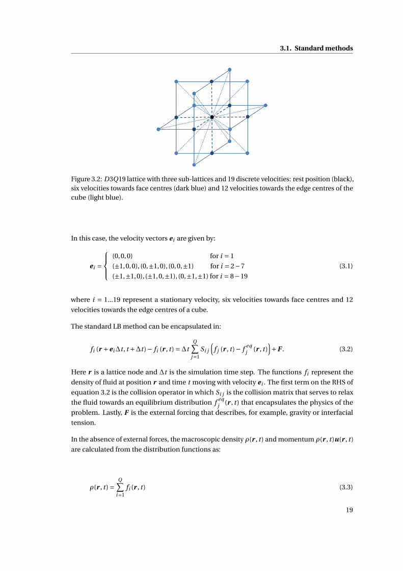
3.1. Standard methods
Figure 3.2: D3Q19 lattice with three sub-lattices and 19 discrete velocities: rest position (black),six velocities towards face centres (dark blue) and 12 velocities towards the edge centres of thecube (light blue).
In this case, the velocity vectors ei are given by:
ei =
(0,0,0) for i = 1
(±1,0,0), (0,±1,0), (0,0,±1) for i = 2−7
(±1,±1,0), (±1,0,±1), (0,±1,±1) for i = 8−19
(3.1)
where i = 1...19 represent a stationary velocity, six velocities towards face centres and 12
velocities towards the edge centres of a cube.
The standard LB method can be encapsulated in:
fi (r +ei∆t , t +∆t )− fi (r , t ) =∆tQ∑
j=1Si j
(f j (r , t )− f eq
j (r , t ))+F . (3.2)
Here r is a lattice node and ∆t is the simulation time step. The functions fi represent the
density of fluid at position r and time t moving with velocity ei . The first term on the RHS of
equation 3.2 is the collision operator in which Si j is the collision matrix that serves to relax
the fluid towards an equilibrium distribution f eqj (r , t) that encapsulates the physics of the
problem. Lastly, F is the external forcing that describes, for example, gravity or interfacial
tension.
In the absence of external forces, the macroscopic density ρ(r , t ) and momentum ρ(r , t )u(r , t )
are calculated from the distribution functions as:
ρ(r , t ) =Q∑
i=1fi (r , t ) (3.3)
19
Chapter 3. Lattice Boltzmann Methods for Isothermal Fluids
and
ρ(r , t )u(r , t ) =Q∑
i=1fi (r , t )ei (3.4)
where u(r , t ) is the macroscopic velocity.
3.1.2 Collision operators and equilibrium functions
The collision operator serves to relax the fluid towards the equilibrium functions. A very
widely used approximation of the collision operator is the Bhatnagar-Gross-Krook (BGK)
model [51], also known as the single-relaxation-time (SRT) model. This model reduces the
collision operator to
Si j =−1
τδi j (3.5)
where τ is the relaxation time and δi j =
0 if i 6= j
1 if i = jis the Kronecker delta. The first term of
the RHS of equation 3.2 becomes:
Q∑j=1
Si j
(f j (r , t )− f eq
j (r , t ))=−1
τ
(fi (r , t )− f eq
i (r , t ))
. (3.6)
The relaxation time τ is related to the kinematic fluid viscosity υ through
υ= c2s
(τ− ∆t
2
)(3.7)
where c2s = c2
3 is the lattice speed of sound with c = ∆x∆t the lattice speed and ∆x the lattice
spacing.
Under certain conditions, the SRT collision operator yields unphysical behaviour such as
viscosity-dependent permeability [63, 64, 65]. To overcome this problem, the multi-relaxation-
time (MRT) scheme [63] was developed. In this version, the linearized collision operator is
implemented in the hydraulic modes of the problem instead of the space of discrete velocities.
The hydraulic modes include hydrodynamic conserved quantities such as the density and
momentum and other non-conserved quantities. The first term of the RHS of equation 3.2
becomes:
Q∑j=1
Si j
(f j (r , t )− f eq
j (r , t ))=−M−1 ·S
(m (r , t )−meq (r , t )
)(3.8)
where S is a diagonal relaxation matrix and M is a 19×19 transformation matrix that links the
20
3.1. Standard methods
hydraulic modes m with the distribution functions f by:
m = M · f (3.9)
f = M−1 ·m. (3.10)
For the D3Q19 lattice, out of the 19 moments, only the density ρ and momentum ( jx , jy , jz )
are conserved and measurable quantities. The other moments can be used to improve the
numerical stability [63] by adjusting their corresponding relaxation times. The MRT model
can be regarded as the more general collision operator, and can be simplified to recovered the
SRT model or a two-relaxation-time (TRT) model as proposed in [64, 65]. More information
about the MRT collision operator can be found in appendix A.
Regardless of the collision operator, the underlying physics of the problem is defined by the
equilibrium distribution functions f eqj . For incompressible isothermal fluids, the equilibrium
distribution functions are [51]:
f eqi (r , t ) =ωiρ
(1+ u∗.ei
c2s
+ (u∗.ei )2
2c4s
− u∗.u∗
2c2s
), (3.11)
where u∗ is the equilibrium velocity and is equal to the macroscopic velocity in absence of
external forcing. The lattice weights ωi are specific to the chosen lattice and are calculated in
order to correct the lattice with respect to isotropy. For the D3Q19 lattice, they are:
ωi =
13 for ei = 0 (i = 1)1
18 for ei = 1 (i = 2−7) .1
36 for ei =p
2 (i = 8−19)
(3.12)
3.1.3 Boundary conditions
Fluid – solid boundaries
In computational fluid dynamics (CFD) models, the collision of the fluid with solid boundaries
is usually accounted for by implementing a no-slip boundary condition. In lattice Boltzmann
methods, the no-slip boundary condition is often approximated with the bounce-back rule
[66]: if a fluid element hits a solid boundary following the propagation step, its momentum is
reversed so that:
fi (r +ei , t +1) = f i (r , t ) (3.13)
where i is the direction opposite to i : ei =−e i . This ability to handle highly irregular bound-
aries by means of simple arithmetical operations is one of the most appealing advantages of
LB methods. The bounce-back rule is the most widely used fluid – solid boundary condition
as it provides a very good compromise between ease of implementation, numerical perfor-
mance and accuracy. The main draw-back of the bounce-back rule is that spherical structures
21
Chapter 3. Lattice Boltzmann Methods for Isothermal Fluids
must be approximated with stair-case geometries (zig-zag type). Consequently, if the lattice
resolution is coarse, the bounce-back rule introduces an artificial rugosity which might reduce
the accuracy of the near-wall flow fields [53].
Open-flow boundaries
Unlike fluid – solid boundaries, open flow boundaries are not physical interfaces. In many
CFD applications, the pressure or the velocity is fixed on a boundary in order to replicate
an experimental condition (e.g. pressure head or wind speed). The former is referred to
as Dirichlet boundary condition and the latter as Neumann boundary condition. In LB
methods, the Dirichlet boundary condition can be replicated by applying a body- force [67] or
by controlling the pressures at the inlet and outlet of the sample [68].
Body-force There are several ways to implement a body-force in lattice Boltzmann algo-
rithms. Most commonly, an external force acting on all the fluid nodes is implemented by
adding a term, i.e. F , to the RHS of equation 3.2 and then modifying the macroscopic and
equilibrium velocities accordingly [67, 68, 69]. Several mathematically derived variants exist.
One variant consists of adding the term [67]
Fi = 3ωi ei .g (3.14)
to the RHS of equation 3.2 where g is the acceleration due to the external forces. The velocities
become:
u (r , t ) = u∗ (r , t ) =∑Q
i=1 fi (r , t )ei∑Qi=1 fi (r , t )
+ g
2(3.15)
where it is assumed that ∆t = 1 and that the average density in the system is ρ0 = 1.
Pressure boundary conditions An alternative way to control the flow takes advantage of
the equation of state that links the pressure P to the density ρ by:
P = c2s ρ. (3.16)
Accordingly, it is possible to define regions with a certain pressure by setting the corresponding
densities in a hydro-dynamically consistent way. Zou and He [68] first proposed how to
implement pressure boundary conditions for the D2Q9 lattice and explained how to derive
them for the D3Q15 lattice. Kutay et al. [70] extended the pressure boundary conditions to
include the D3Q19 lattice. Most recently, Hecht and Harting [71] generalized the condition
to include inflow with arbitrary velocity direction on D3Q19 lattices. The pressure boundary
conditions are derived for LB algorithms by using the density and momentum equations. Due
to the continuity relation, it is possible to specify three of the four variables(ρ,ux ,uy ,uz
)and
22
3.1. Standard methods
then solve for the fourth. Since the density must be fixed in order to control the pressure, it is
possible to fix two out of the three components of the velocity. For example, in the most simple
case, a pressure can be imposed by setting ρ = ρ0, uy = uz = 0 and then solving for ux . All of
this is done by calculating and setting the appropriate values of the distribution functions.
More information about pressure boundary conditions can be found in appendix B.
3.1.4 Definition of a lattice Boltzmann algorithm
A lattice Boltzmann algorithm consists of a combination of:
1. A set of equilibrium distribution functions that defines the physics of the problem (e.g.
isothermal or non-ideal fluids).
2. A fluid – fluid collision operator that relaxes the system towards the equilibrium distri-
bution functions.
3. A fluid – solid boundary condition that describes the interactions between the fluid and
the solid (e.g. no-slip, wetting).
4. An open-flow boundary condition that replicates the experimental conditions (e.g.
pressure head, gravity, wind speed, ambient relative humidity).
Finally, the algorithm is implemented in a computer program with an implementation lan-
guage.
3.1.5 Implementation
As part of this work, a lattice Boltzmann algorithm was implemented to simulate the per-
meation of isothermal fluids in saturated porous media. The equilibrium distribution func-
tions were defined with equation 3.11 to model an incompressible isothermal fluid. A multi-
relaxation-time collision operator was implemented as developed by D’Humières et al. [63]
and described in appendix A. The relaxation rates were chosen following the two-relaxation-
time model [64, 65] so that:
s1 = s4 = s6 = s8 = 0,
s2 = s3 = s10 = s11 = s12 = s13 = s14 = s15 = s16 = 1/τ,
s5 = s7 = s9 = s17 = s18 = s19 = 8(2− s2)/
(8− s2).
(3.17)
The main relaxation time was set to τ= 0.6 following the work of Ref. [69] on the permeability
of Fontainebleau sandstones. The no-slip fluid-solid boundary condition was simulated by
applying the standard bounce-back rule. The pressure gradient driving the fluid was simulated
with an external force acting on all fluid nodes. The acceleration in equation 3.14 was set to
g = g ex where the acceleration value, g , was set to 10−5. Periodic boundary conditions were
23
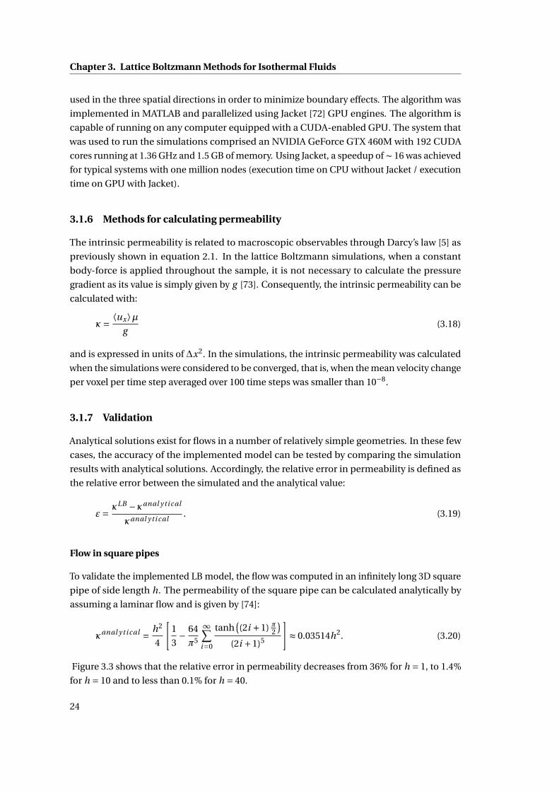
Chapter 3. Lattice Boltzmann Methods for Isothermal Fluids
used in the three spatial directions in order to minimize boundary effects. The algorithm was
implemented in MATLAB and parallelized using Jacket [72] GPU engines. The algorithm is
capable of running on any computer equipped with a CUDA-enabled GPU. The system that
was used to run the simulations comprised an NVIDIA GeForce GTX 460M with 192 CUDA
cores running at 1.36 GHz and 1.5 GB of memory. Using Jacket, a speedup of ∼ 16 was achieved
for typical systems with one million nodes (execution time on CPU without Jacket / execution
time on GPU with Jacket).
3.1.6 Methods for calculating permeability
The intrinsic permeability is related to macroscopic observables through Darcy’s law [5] as
previously shown in equation 2.1. In the lattice Boltzmann simulations, when a constant
body-force is applied throughout the sample, it is not necessary to calculate the pressure
gradient as its value is simply given by g [73]. Consequently, the intrinsic permeability can be
calculated with:
κ= ⟨ux⟩µg
(3.18)
and is expressed in units of ∆x2. In the simulations, the intrinsic permeability was calculated
when the simulations were considered to be converged, that is, when the mean velocity change
per voxel per time step averaged over 100 time steps was smaller than 10−8.
3.1.7 Validation
Analytical solutions exist for flows in a number of relatively simple geometries. In these few
cases, the accuracy of the implemented model can be tested by comparing the simulation
results with analytical solutions. Accordingly, the relative error in permeability is defined as
the relative error between the simulated and the analytical value:
ε= κLB −κanal y ti cal
κanal y ti cal. (3.19)
Flow in square pipes
To validate the implemented LB model, the flow was computed in an infinitely long 3D square
pipe of side length h. The permeability of the square pipe can be calculated analytically by
assuming a laminar flow and is given by [74]:
κanal y ti cal = h2
4
[1
3− 64
π5
∞∑i=0
tanh((2i +1) π2
)(2i +1)5
]≈ 0.03514h2. (3.20)
Figure 3.3 shows that the relative error in permeability decreases from 36% for h = 1, to 1.4%
for h = 10 and to less than 0.1% for h = 40.
24
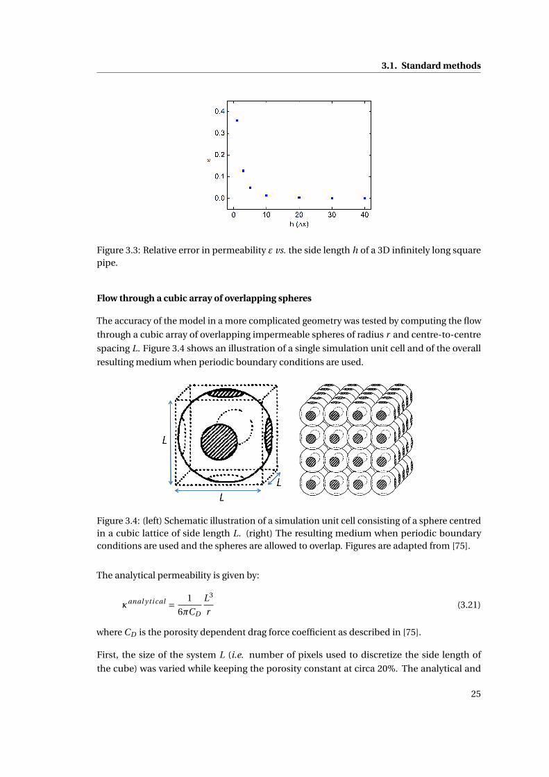
3.1. Standard methods
Figure 3.3: Relative error in permeability ε vs. the side length h of a 3D infinitely long squarepipe.
Flow through a cubic array of overlapping spheres
The accuracy of the model in a more complicated geometry was tested by computing the flow
through a cubic array of overlapping impermeable spheres of radius r and centre-to-centre
spacing L. Figure 3.4 shows an illustration of a single simulation unit cell and of the overall
resulting medium when periodic boundary conditions are used.
Figure 3.4: (left) Schematic illustration of a simulation unit cell consisting of a sphere centredin a cubic lattice of side length L. (right) The resulting medium when periodic boundaryconditions are used and the spheres are allowed to overlap. Figures are adapted from [75].
The analytical permeability is given by:
κanal y ti cal = 1
6πCD
L3
r(3.21)
where CD is the porosity dependent drag force coefficient as described in [75].
First, the size of the system L (i.e. number of pixels used to discretize the side length of
the cube) was varied while keeping the porosity constant at circa 20%. The analytical and
25
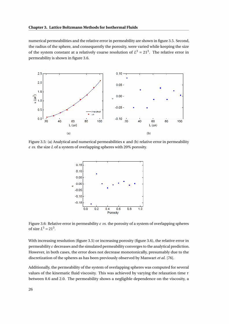
Chapter 3. Lattice Boltzmann Methods for Isothermal Fluids
numerical permeabilities and the relative error in permeability are shown in figure 3.5. Second,
the radius of the sphere, and consequently the porosity, were varied while keeping the size
of the system constant at a relatively coarse resolution of L3 = 213. The relative error in
permeability is shown in figure 3.6.
(a) (b)
Figure 3.5: (a) Analytical and numerical permeabilities κ and (b) relative error in permeabilityε vs. the size L of a system of overlapping spheres with 20% porosity.
Figure 3.6: Relative error in permeability ε vs. the porosity of a system of overlapping spheresof size L3 = 213.
With increasing resolution (figure 3.5) or increasing porosity (figure 3.6), the relative error in
permeability ε decreases and the simulated permeability converges to the analytical prediction.
However, in both cases, the error does not decrease monotonically, presumably due to the
discretization of the spheres as has been previously observed by Manwart et al. [76].
Additionally, the permeability of the system of overlapping spheres was computed for several
values of the kinematic fluid viscosity. This was achieved by varying the relaxation time τ
between 0.6 and 2.0. The permeability shows a negligible dependence on the viscosity, a
26
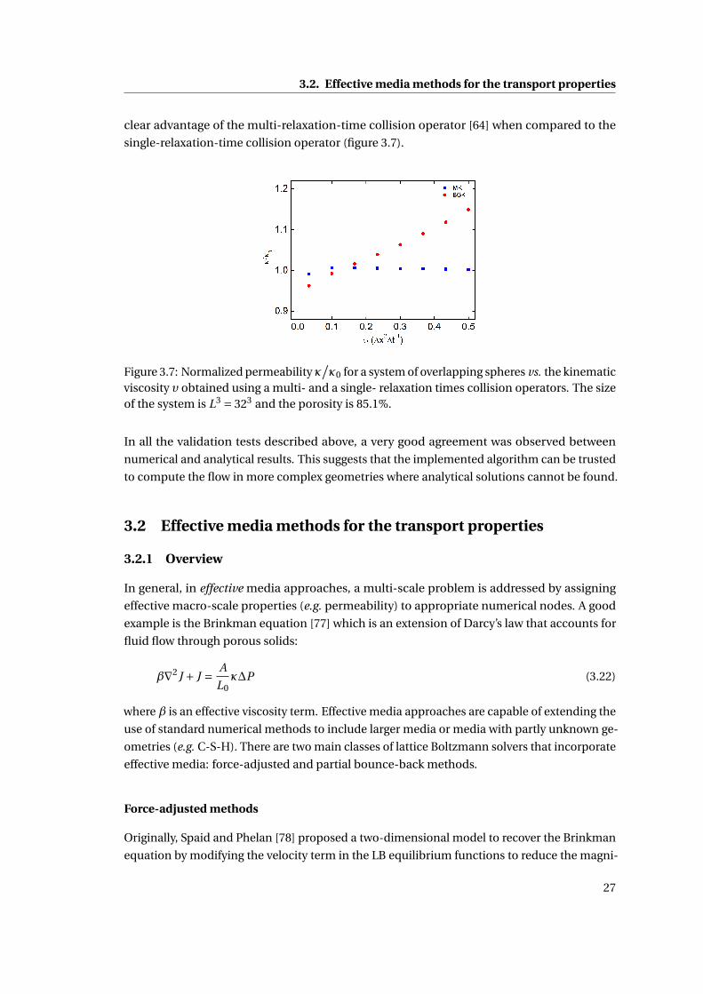
3.2. Effective media methods for the transport properties
clear advantage of the multi-relaxation-time collision operator [64] when compared to the
single-relaxation-time collision operator (figure 3.7).
Figure 3.7: Normalized permeabilityκ/κ0 for a system of overlapping spheres vs. the kinematic
viscosity υ obtained using a multi- and a single- relaxation times collision operators. The sizeof the system is L3 = 323 and the porosity is 85.1%.
In all the validation tests described above, a very good agreement was observed between
numerical and analytical results. This suggests that the implemented algorithm can be trusted
to compute the flow in more complex geometries where analytical solutions cannot be found.
3.2 Effective media methods for the transport properties
3.2.1 Overview
In general, in effective media approaches, a multi-scale problem is addressed by assigning
effective macro-scale properties (e.g. permeability) to appropriate numerical nodes. A good
example is the Brinkman equation [77] which is an extension of Darcy’s law that accounts for
fluid flow through porous solids:
β∇2 J + J = A
L0κ∆P (3.22)
where β is an effective viscosity term. Effective media approaches are capable of extending the
use of standard numerical methods to include larger media or media with partly unknown ge-
ometries (e.g. C-S-H). There are two main classes of lattice Boltzmann solvers that incorporate
effective media: force-adjusted and partial bounce-back methods.
Force-adjusted methods
Originally, Spaid and Phelan [78] proposed a two-dimensional model to recover the Brinkman
equation by modifying the velocity term in the LB equilibrium functions to reduce the magni-
27
Chapter 3. Lattice Boltzmann Methods for Isothermal Fluids
tude of the momentum. The idea behind this approach is to use the Stokes equation to model
the flow in open regions, and the Brinkman equation to model the flow through porous struc-
tures by treating them as an effective medium of known permeability. The main drawback of
this approach is its inability to model objects with very low permeability. Freed [79] improved
the method by allowing it to recover flow through a resistance field with a higher momentum
sink. Martys [80] extended the validity of the LB Stokes-Brinkman approach over a larger range
of forcing and “porous media effective viscosity” by incorporating the dissipative forcing into
a linear body-force. Martys and Hagedorn [81] applied this model to study the effect of the
permeability of sand grains on the bulk permeability of a Fontainebleau sandstone. Unsurpris-
ingly, they found that the bulk permeability increases with the sand grain permeability at low
porosities, and that, at high porosities, the bulk permeability is insensitive to the sand grain
permeability. They pointed out that their algorithm was unstable when the sand permeability
was low, less than order∗ ∼ 0.1∆x2. Kang et al. [7] combined the Stokes-Brinkman LB model
with a non-uniform mesh to study the effect of simplified 2D fractures on the permeability
of rocks. They reported that the importance of the flow in the porous matrix depends on the
ratio of the permeability of the porous matrix to that of the fracture.
Partial bounce-back methods
In a different approach based on earlier work done by Balasubramanian et al. [82] and Gao
and Sharma [83] on lattice gases, Dardis and McCloskey [84, 85] proposed a lattice Boltzmann
method where momentum loss is due to the “presence of solid obstacles”. The “solid scatterer
density”, or more simply the “solid fraction”, is related to the permeability of the porous
medium that they represent. They reported a behaviour consistent with a Kozeny-Carman [86,
87] type relationship between the solid fraction and the permeability for low to intermediate
solid fractions. They noted that at intermediate to high solid fractions, the rapid decrease in
permeability is consistent with a percolation process giving a power-law relationship between
the solid fraction and the permeability. However, their use of a two-dimensional hexagonal
lattice made it impossible to calculate the permeability of porous media with high solid
fractions and thus low permeabilities. Thorne and Sukop [88, 89] developed an algorithm
where the additional “porous media step” takes place after the traditional collision step and
used it on a D2Q9 lattice to model the Elder problem where the fluid flow is initiated by density
variations. Chen and Zhu [90] analysed the Gao and Sharma [83], Dardis and McCloskey
[84] and Thorne and Sukop [88] models. They showed that only the Thorne and Sukop
model is valid for the whole range of solid fractions (zero to one). They also showed that
these models yielded velocity profiles in good agreement with Brinkman’s predictions. Walsh
et al. [91] proposed a new “pre-collision” partial bounce-back algorithm and derived an
analytical expression that links the permeability to the “solid fraction”. They showed that
their model [91] and the models of Dardis and McCloskey [84] and Thorne and Sukop [88]
produce equivalent results although their own has significant advantages in terms of mass
conservation in heterogeneous media and suitability for parallel computing. Recently, Zhu
∗In general, ∆x is on the order of 10−7 to 10−5 m in porous media.
28
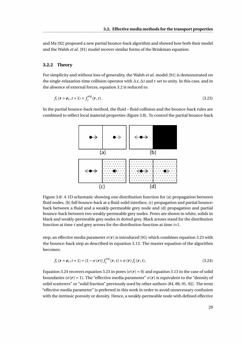
3.2. Effective media methods for the transport properties
and Ma [92] proposed a new partial bounce-back algorithm and showed how both their model
and the Walsh et al. [91] model recover similar forms of the Brinkman equation.
3.2.2 Theory
For simplicity and without loss of generality, the Walsh et al. model [91] is demonstrated on
the single-relaxation-time collision operator with ∆x,∆t and τ set to unity. In this case, and in
the absence of external forces, equation 3.2 is reduced to:
fi (r +ei , t +1) = f eqi (r , t ) . (3.23)
In the partial bounce-back method, the fluid – fluid collision and the bounce-back rules are
combined to reflect local material properties (figure 3.8). To control the partial bounce-back
Figure 3.8: A 1D schematic showing one distribution function for (a) propagation betweenfluid nodes, (b) full bounce-back at a fluid-solid interface, (c) propagation and partial bounce-back between a fluid and a weakly-permeable grey node and (d) propagation and partialbounce-back between two weakly-permeable grey nodes. Pores are shown in white, solids inblack and weakly-permeable grey nodes in dotted grey. Black arrows stand for the distributionfunction at time t and grey arrows for the distribution function at time t+1.
step, an effective media parameter σ(r ) is introduced [91] which combines equation 3.23 with
the bounce-back step as described in equation 3.13. The master equation of the algorithm
becomes:
fi (r +ei , t +1) = [1−σ (r )] f eqi (r , t )+σ (r ) f i (r , t ) . (3.24)
Equation 3.24 recovers equation 3.23 in pores (σ(r ) = 0) and equation 3.13 in the case of solid
boundaries (σ(r ) = 1). The “effective media parameter” σ(r ) is equivalent to the “density of
solid scatterers” or “solid fraction” previously used by other authors [84, 88, 91, 92]. The term
“effective media parameter” is preferred in this work in order to avoid unnecessary confusion
with the intrinsic porosity or density. Hence, a weakly-permeable node with defined effective
29
Chapter 3. Lattice Boltzmann Methods for Isothermal Fluids
media properties is labelled a grey node. Accordingly, the following classes of nodes are
defined:
σ(r ) = 0 :
0 <σ(r ) < 1 :
σ(r ) = 1 :
pores
grey nodes
solids
(3.25)
The microscopic and macroscopic density and momentum are given by:
ρ∗(r , t ) =Q∑
i=1fi (r , t ) (3.26)
ρ (r , t ) = [1−σ (r )]Q∑
i=1fi (r , t ) (3.27)
ρ∗ (r , t )u∗ (r , t ) =Q∑
i=1fi (r , t )ei (3.28)
ρ (r , t )u (r , t ) = [1−σ (r )]Q∑
i=1fi (r , t )ei (3.29)
where the asterix signifies a microscopic variable used for the calculation of the equilibrium
functions. For σ(r ) = 0, equations 3.27 and 3.29 recover equations 3.26 and 3.28, respectively
while for σ(r ) = 1 they are both equal to zero.
At the start of each simulation, the nodes are initialized to a microscopic density according to:
ρ∗(r , t = 0) =
0 for solids
1 for grey nodes,
1 for pores
(3.30)
zero microscopic velocity:
u∗(r , t = 0) = 0, (3.31)
and the macroscopic moments are calculated with equations 3.27 and 3.29.
Walsh et al. [91] derived the intrinsic permeability of grey nodes (partially-permeable homo-
geneous media for which σ(r ) =σ∀r ) as a function of the fluid kinematic viscosity and the
effective media parameter as:
κ(r ) = 1−σ(r )
2σ(r )υ. (3.32)
Equation 3.32 was derived by projecting the D3Q19 lattice onto a D1Q3 lattice and assuming
a stationary fluid as shown in Appendix C. For low values of the effective media parameter σ,
a similar equation, κ= υ/2σ, was obtained by Balasubramanian et al. [82] by introducing a
damping term proportional to the velocity in the Navier-Stokes equation.
30
3.2. Effective media methods for the transport properties
3.2.3 Implementation
The model as described above in equation 3.24 was first proposed and implemented by
Walsh et al. in 2D [91]. What follows is believed to be the first 3D implementation. A three-
dimensional version is necessary for porous media because the percolation is critically de-
pendent on the number of spatial dimensions. This implementation will highlight some
ambiguities within [91], demonstrate the ability of the model in a number of relatively com-
plex geometries, and compare the numerical results with analytical predictions whenever
possible.
Walsh et al. use the term “solid fraction”. In this work, the term “effective media parameter” is
preferred in order to avoid any unnecessary confusion with the inherent porosity or density of
the grey nodes.
Walsh et al. tested the model on homogeneous materials composed of grey nodes only.
Although Walsh and Saar [93] subsequently studied the 2D speleogenesis of carbonate aquifers
with a wide range of permeabilities, it was an application and not a validation and hence it did
not clarify the implementation method. The setups used by Walsh et al. [91] are insufficient to
reveal errors or inconsistencies in the definition of the hydrodynamic moments. This became
clear as soon as inhomogeneous materials with pores, grey nodes and solids were tested.
This is the reason why Zhu and Ma [92] recently claimed that, in the Walsh et al. model, the
velocity appears to be “discontinuous” at the interfaces between grey nodes with different
permeabilities. However, equations 3.24 - 3.31 show, clearly, how to implement the model and
initialize the variables. Section 3.2.5 demonstrates the accuracy of the model in a wide range
of test setups. Additionally, section 3.2.5 shows that the “discontinuities” reported by Zhu and
Ma are not a property or a limitation of the Walsh et al. model. Rather, they are most probably
due to an inconsistency in the implementation of the Walsh et al. model by Zhu and Ma.
As part of this work, an effective media lattice Boltzmann model was implemented to simulate
the permeation of isothermal fluids in saturated porous media. The equilibrium distribution
functions were defined with equation 3.11 to model an incompressible isothermal fluid.
The single-relaxation-time was preferred to the multi-relaxation-time collision operator to
minimize the number of parameters while developing the model. For numerical efficiency,
the relaxation time was set to τ= 1. The no-slip fluid-solid boundary condition was taken into
account in an implicit way in equation 3.24 on solid boundaries marked with σ(r ) = 1. The
pressure gradient driving the fluid was simulated with pressure boundary conditions acting
inside injection chambers as further discussed below. Periodic boundary conditions were
used in the two remaining spatial directions in order to minimize boundary effects. Finally,
the effective media algorithm was written in C and parallelized using the OpenMP library.
31
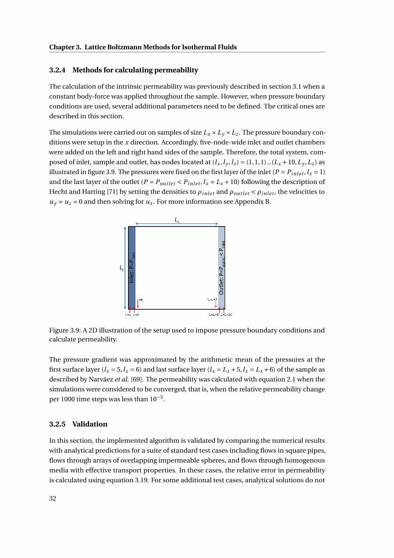
Chapter 3. Lattice Boltzmann Methods for Isothermal Fluids
3.2.4 Methods for calculating permeability
The calculation of the intrinsic permeability was previously described in section 3.1 when a
constant body-force was applied throughout the sample. However, when pressure boundary
conditions are used, several additional parameters need to be defined. The critical ones are
described in this section.
The simulations were carried out on samples of size Lx ×Ly ×Lz . The pressure boundary con-
ditions were setup in the x direction. Accordingly, five-node-wide inlet and outlet chambers
were added on the left and right hand sides of the sample. Therefore, the total system, com-
posed of inlet, sample and outlet, has nodes located at (lx , ly , lz ) = (1,1,1)...(Lx +10,Ly ,Lz ) as
illustrated in figure 3.9. The pressures were fixed on the first layer of the inlet (P = Pi nlet , lx = 1)
and the last layer of the outlet (P = Poutlet < Pi nlet , lx = Lx +10) following the description of
Hecht and Harting [71] by setting the densities to ρi nlet and ρoutlet < ρi nlet , the velocities to
uy = uz = 0 and then solving for ux . For more information see Appendix B.
Figure 3.9: A 2D illustration of the setup used to impose pressure boundary conditions andcalculate permeability.
The pressure gradient was approximated by the arithmetic mean of the pressures at the
first surface layer (lx = 5, lx = 6) and last surface layer (lx = Lx +5, lx = Lx +6) of the sample as
described by Narváez et al. [69]. The permeability was calculated with equation 2.1 when the
simulations were considered to be converged, that is, when the relative permeability change
per 1000 time steps was less than 10−5.
3.2.5 Validation
In this section, the implemented algorithm is validated by comparing the numerical results
with analytical predictions for a suite of standard test cases including flows in square pipes,
flows through arrays of overlapping impermeable spheres, and flows through homogenous
media with effective transport properties. In these cases, the relative error in permeability
is calculated using equation 3.19. For some additional test cases, analytical solutions do not
32
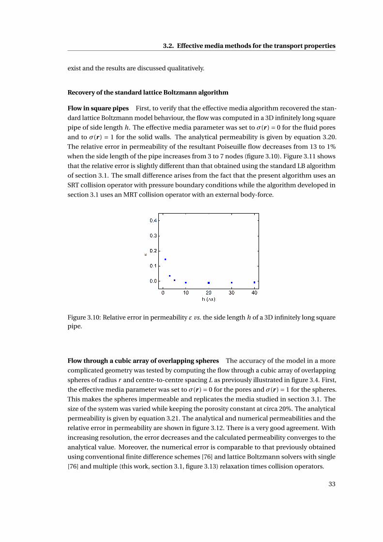
3.2. Effective media methods for the transport properties
exist and the results are discussed qualitatively.
Recovery of the standard lattice Boltzmann algorithm
Flow in square pipes First, to verify that the effective media algorithm recovered the stan-
dard lattice Boltzmann model behaviour, the flow was computed in a 3D infinitely long square
pipe of side length h. The effective media parameter was set to σ(r ) = 0 for the fluid pores
and to σ(r ) = 1 for the solid walls. The analytical permeability is given by equation 3.20.
The relative error in permeability of the resultant Poiseuille flow decreases from 13 to 1%
when the side length of the pipe increases from 3 to 7 nodes (figure 3.10). Figure 3.11 shows
that the relative error is slightly different than that obtained using the standard LB algorithm
of section 3.1. The small difference arises from the fact that the present algorithm uses an
SRT collision operator with pressure boundary conditions while the algorithm developed in
section 3.1 uses an MRT collision operator with an external body-force.
Figure 3.10: Relative error in permeability ε vs. the side length h of a 3D infinitely long squarepipe.
Flow through a cubic array of overlapping spheres The accuracy of the model in a more
complicated geometry was tested by computing the flow through a cubic array of overlapping
spheres of radius r and centre-to-centre spacing L as previously illustrated in figure 3.4. First,
the effective media parameter was set to σ(r ) = 0 for the pores and σ(r ) = 1 for the spheres.
This makes the spheres impermeable and replicates the media studied in section 3.1. The
size of the system was varied while keeping the porosity constant at circa 20%. The analytical
permeability is given by equation 3.21. The analytical and numerical permeabilities and the
relative error in permeability are shown in figure 3.12. There is a very good agreement. With
increasing resolution, the error decreases and the calculated permeability converges to the
analytical value. Moreover, the numerical error is comparable to that previously obtained
using conventional finite difference schemes [76] and lattice Boltzmann solvers with single
[76] and multiple (this work, section 3.1, figure 3.13) relaxation times collision operators.
33
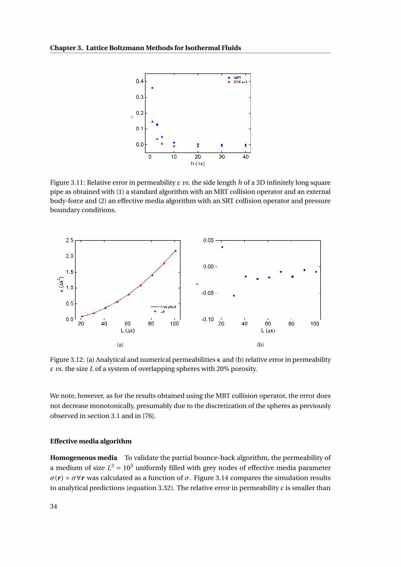
Chapter 3. Lattice Boltzmann Methods for Isothermal Fluids
Figure 3.11: Relative error in permeability ε vs. the side length h of a 3D infinitely long squarepipe as obtained with (1) a standard algorithm with an MRT collision operator and an externalbody-force and (2) an effective media algorithm with an SRT collision operator and pressureboundary conditions.
(a) (b)
Figure 3.12: (a) Analytical and numerical permeabilities κ and (b) relative error in permeabilityε vs. the size L of a system of overlapping spheres with 20% porosity.
We note, however, as for the results obtained using the MRT collision operator, the error does
not decrease monotonically, presumably due to the discretization of the spheres as previously
observed in section 3.1 and in [76].
Effective media algorithm
Homogeneous media To validate the partial bounce-back algorithm, the permeability of
a medium of size L3 = 103 uniformly filled with grey nodes of effective media parameter
σ(r ) = σ∀r was calculated as a function of σ. Figure 3.14 compares the simulation results
to analytical predictions (equation 3.32). The relative error in permeability ε is smaller than
34
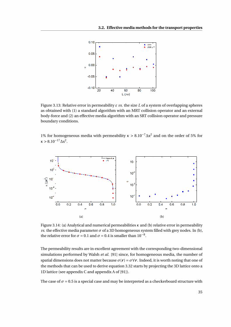
3.2. Effective media methods for the transport properties
Figure 3.13: Relative error in permeability ε vs. the size L of a system of overlapping spheresas obtained with (1) a standard algorithm with an MRT collision operator and an externalbody-force and (2) an effective media algorithm with an SRT collision operator and pressureboundary conditions.
1% for homogeneous media with permeability κ > 8.10−7∆x2 and on the order of 5% for
κ> 8.10−17∆x2.
(a) (b)
Figure 3.14: (a) Analytical and numerical permeabilities κ and (b) relative error in permeabilityvs. the effective media parameter σ of a 3D homogeneous system filled with grey nodes. In (b),the relative error for σ= 0.1 and σ= 0.4 is smaller than 10−8.
The permeability results are in excellent agreement with the corresponding two-dimensional
simulations performed by Walsh et al. [91] since, for homogeneous media, the number of
spatial dimensions does not matter because σ(r ) =σ∀r . Indeed, it is worth noting that one of
the methods that can be used to derive equation 3.32 starts by projecting the 3D lattice onto a
1D lattice (see appendix C and appendix A of [91]).
The case of σ= 0.5 is a special case and may be interpreted as a checkerboard structure with
35
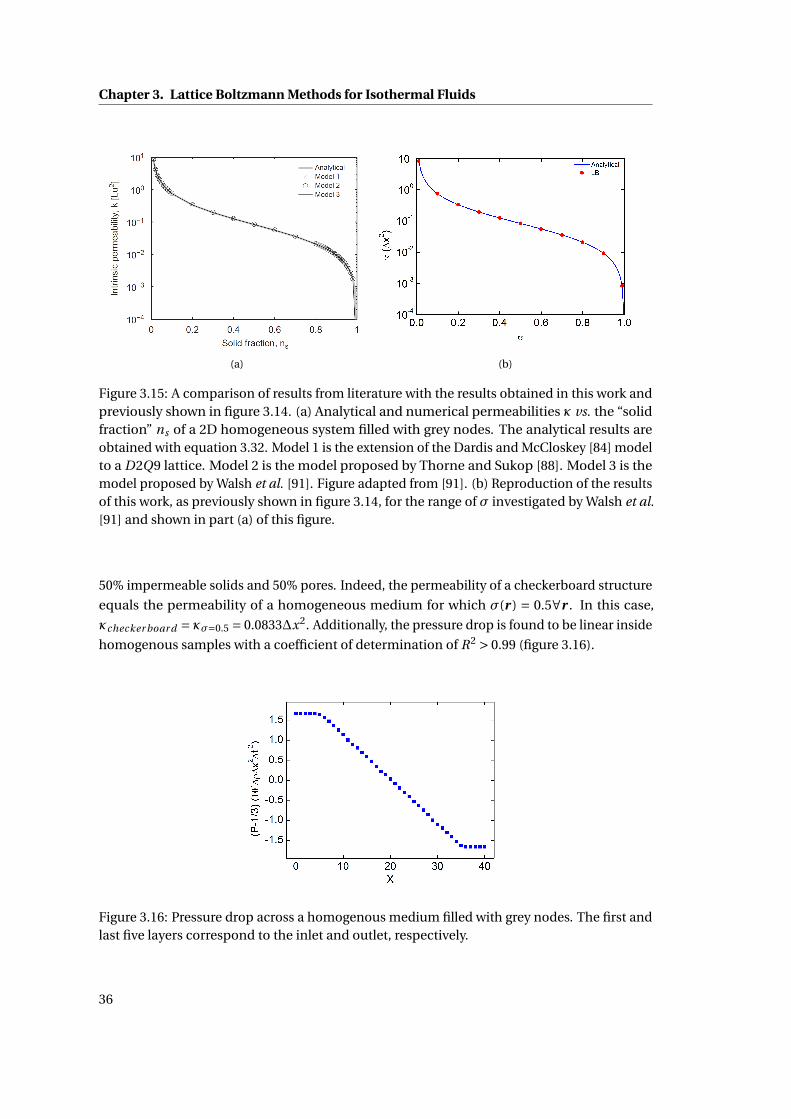
Chapter 3. Lattice Boltzmann Methods for Isothermal Fluids
(a) (b)
Figure 3.15: A comparison of results from literature with the results obtained in this work andpreviously shown in figure 3.14. (a) Analytical and numerical permeabilities κ vs. the “solidfraction” ns of a 2D homogeneous system filled with grey nodes. The analytical results areobtained with equation 3.32. Model 1 is the extension of the Dardis and McCloskey [84] modelto a D2Q9 lattice. Model 2 is the model proposed by Thorne and Sukop [88]. Model 3 is themodel proposed by Walsh et al. [91]. Figure adapted from [91]. (b) Reproduction of the resultsof this work, as previously shown in figure 3.14, for the range of σ investigated by Walsh et al.[91] and shown in part (a) of this figure.
50% impermeable solids and 50% pores. Indeed, the permeability of a checkerboard structure
equals the permeability of a homogeneous medium for which σ(r ) = 0.5∀r . In this case,
κchecker boar d = κσ=0.5 = 0.0833∆x2. Additionally, the pressure drop is found to be linear inside
homogenous samples with a coefficient of determination of R2 > 0.99 (figure 3.16).
Figure 3.16: Pressure drop across a homogenous medium filled with grey nodes. The first andlast five layers correspond to the inlet and outlet, respectively.
36
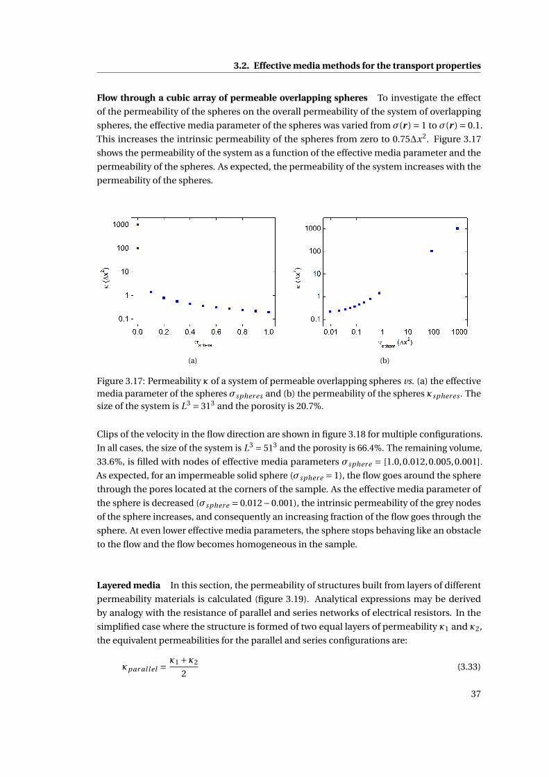
3.2. Effective media methods for the transport properties
Flow through a cubic array of permeable overlapping spheres To investigate the effect
of the permeability of the spheres on the overall permeability of the system of overlapping
spheres, the effective media parameter of the spheres was varied from σ(r ) = 1 to σ(r ) = 0.1.
This increases the intrinsic permeability of the spheres from zero to 0.75∆x2. Figure 3.17
shows the permeability of the system as a function of the effective media parameter and the
permeability of the spheres. As expected, the permeability of the system increases with the
permeability of the spheres.
(a) (b)
Figure 3.17: Permeability κ of a system of permeable overlapping spheres vs. (a) the effectivemedia parameter of the spheres σspher es and (b) the permeability of the spheres κspher es . Thesize of the system is L3 = 313 and the porosity is 20.7%.
Clips of the velocity in the flow direction are shown in figure 3.18 for multiple configurations.
In all cases, the size of the system is L3 = 513 and the porosity is 66.4%. The remaining volume,
33.6%, is filled with nodes of effective media parameters σspher e = [1.0,0.012,0.005,0.001].
As expected, for an impermeable solid sphere (σspher e = 1), the flow goes around the sphere
through the pores located at the corners of the sample. As the effective media parameter of
the sphere is decreased (σspher e = 0.012−0.001), the intrinsic permeability of the grey nodes
of the sphere increases, and consequently an increasing fraction of the flow goes through the
sphere. At even lower effective media parameters, the sphere stops behaving like an obstacle
to the flow and the flow becomes homogeneous in the sample.
Layered media In this section, the permeability of structures built from layers of different
permeability materials is calculated (figure 3.19). Analytical expressions may be derived
by analogy with the resistance of parallel and series networks of electrical resistors. In the
simplified case where the structure is formed of two equal layers of permeability κ1 and κ2,
the equivalent permeabilities for the parallel and series configurations are:
κpar al l el =κ1 +κ2
2(3.33)
37
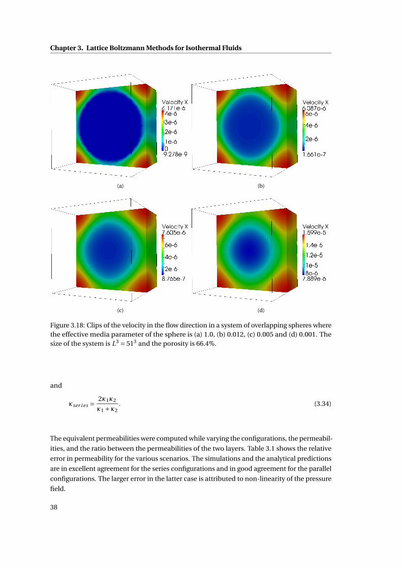
Chapter 3. Lattice Boltzmann Methods for Isothermal Fluids
(a) (b)
(c) (d)
Figure 3.18: Clips of the velocity in the flow direction in a system of overlapping spheres wherethe effective media parameter of the sphere is (a) 1.0, (b) 0.012, (c) 0.005 and (d) 0.001. Thesize of the system is L3 = 513 and the porosity is 66.4%.
and
κser i es = 2κ1κ2
κ1 +κ2. (3.34)
The equivalent permeabilities were computed while varying the configurations, the permeabil-
ities, and the ratio between the permeabilities of the two layers. Table 3.1 shows the relative
error in permeability for the various scenarios. The simulations and the analytical predictions
are in excellent agreement for the series configurations and in good agreement for the parallel
configurations. The larger error in the latter case is attributed to non-linearity of the pressure
field.
38
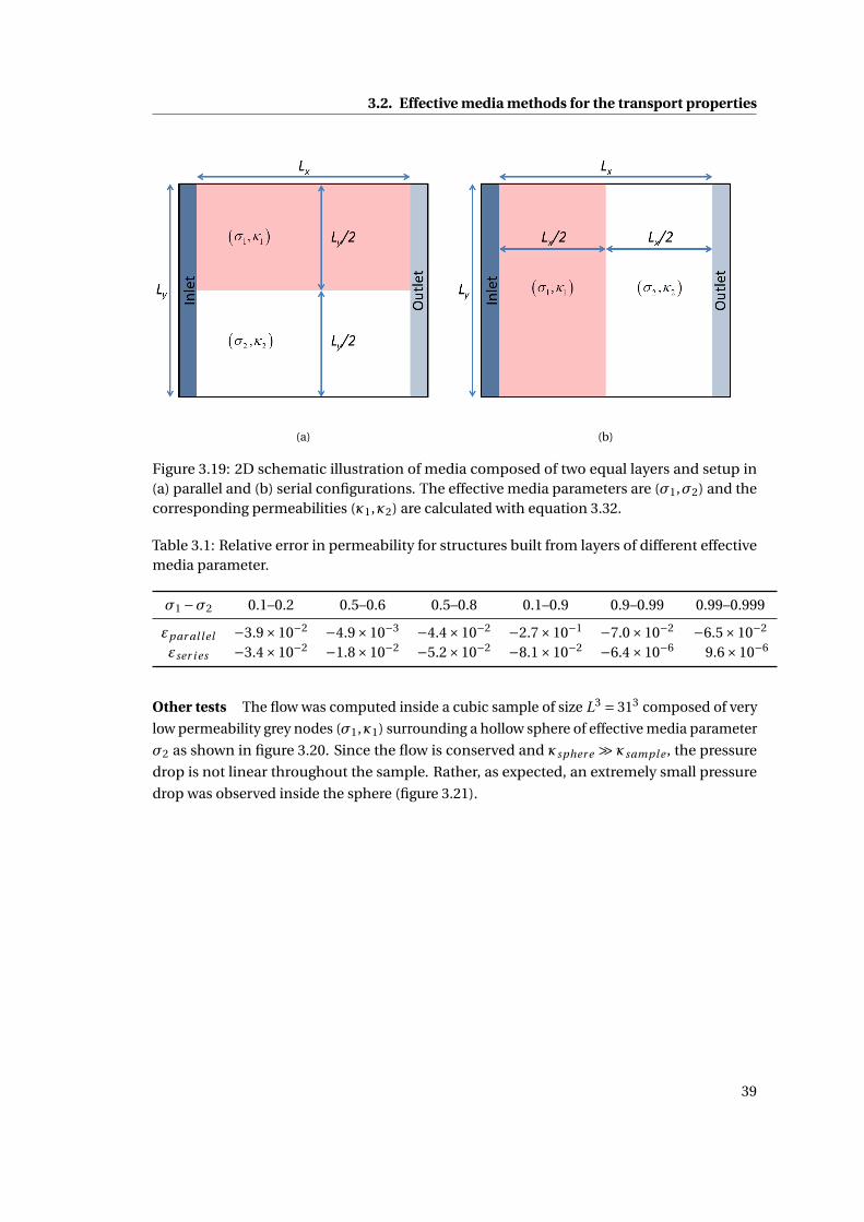
3.2. Effective media methods for the transport properties
(a) (b)
Figure 3.19: 2D schematic illustration of media composed of two equal layers and setup in(a) parallel and (b) serial configurations. The effective media parameters are (σ1,σ2) and thecorresponding permeabilities (κ1,κ2) are calculated with equation 3.32.
Table 3.1: Relative error in permeability for structures built from layers of different effectivemedia parameter.
σ1 −σ2 0.1–0.2 0.5–0.6 0.5–0.8 0.1–0.9 0.9–0.99 0.99–0.999
εpar al l el −3.9×10⁻² −4.9×10⁻³ −4.4×10⁻² −2.7×10⁻¹ −7.0×10⁻² −6.5×10⁻²
εser i es −3.4×10⁻² −1.8×10⁻² −5.2×10⁻² −8.1×10⁻² −6.4×10⁻⁶ 9.6×10⁻⁶
Other tests The flow was computed inside a cubic sample of size L3 = 313 composed of very
low permeability grey nodes (σ1,κ1) surrounding a hollow sphere of effective media parameter
σ2 as shown in figure 3.20. Since the flow is conserved and κspher e À κsample , the pressure
drop is not linear throughout the sample. Rather, as expected, an extremely small pressure
drop was observed inside the sphere (figure 3.21).
39
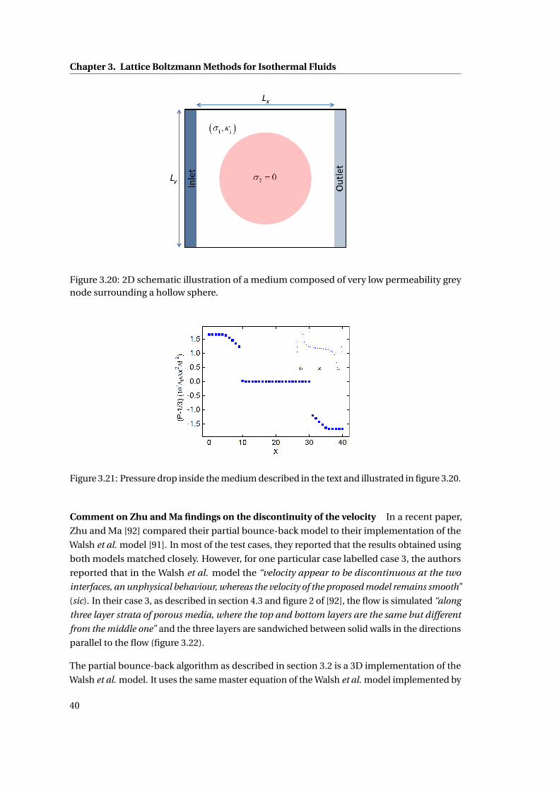
Chapter 3. Lattice Boltzmann Methods for Isothermal Fluids
Figure 3.20: 2D schematic illustration of a medium composed of very low permeability greynode surrounding a hollow sphere.
Figure 3.21: Pressure drop inside the medium described in the text and illustrated in figure 3.20.
Comment on Zhu and Ma findings on the discontinuity of the velocity In a recent paper,
Zhu and Ma [92] compared their partial bounce-back model to their implementation of the
Walsh et al. model [91]. In most of the test cases, they reported that the results obtained using
both models matched closely. However, for one particular case labelled case 3, the authors
reported that in the Walsh et al. model the “velocity appear to be discontinuous at the two
interfaces, an unphysical behaviour, whereas the velocity of the proposed model remains smooth”
(sic). In their case 3, as described in section 4.3 and figure 2 of [92], the flow is simulated “along
three layer strata of porous media, where the top and bottom layers are the same but different
from the middle one” and the three layers are sandwiched between solid walls in the directions
parallel to the flow (figure 3.22).
The partial bounce-back algorithm as described in section 3.2 is a 3D implementation of the
Walsh et al. model. It uses the same master equation of the Walsh et al. model implemented by
40
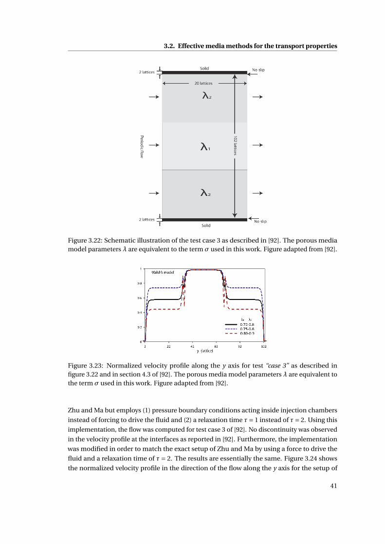
3.2. Effective media methods for the transport properties
Figure 3.22: Schematic illustration of the test case 3 as described in [92]. The porous mediamodel parameters λ are equivalent to the term σ used in this work. Figure adapted from [92].
Figure 3.23: Normalized velocity profile along the y axis for test “case 3” as described infigure 3.22 and in section 4.3 of [92]. The porous media model parameters λ are equivalent tothe term σ used in this work. Figure adapted from [92].
Zhu and Ma but employs (1) pressure boundary conditions acting inside injection chambers
instead of forcing to drive the fluid and (2) a relaxation time τ= 1 instead of τ= 2. Using this
implementation, the flow was computed for test case 3 of [92]. No discontinuity was observed
in the velocity profile at the interfaces as reported in [92]. Furthermore, the implementation
was modified in order to match the exact setup of Zhu and Ma by using a force to drive the
fluid and a relaxation time of τ= 2. The results are essentially the same. Figure 3.24 shows
the normalized velocity profile in the direction of the flow along the y axis for the setup of
41
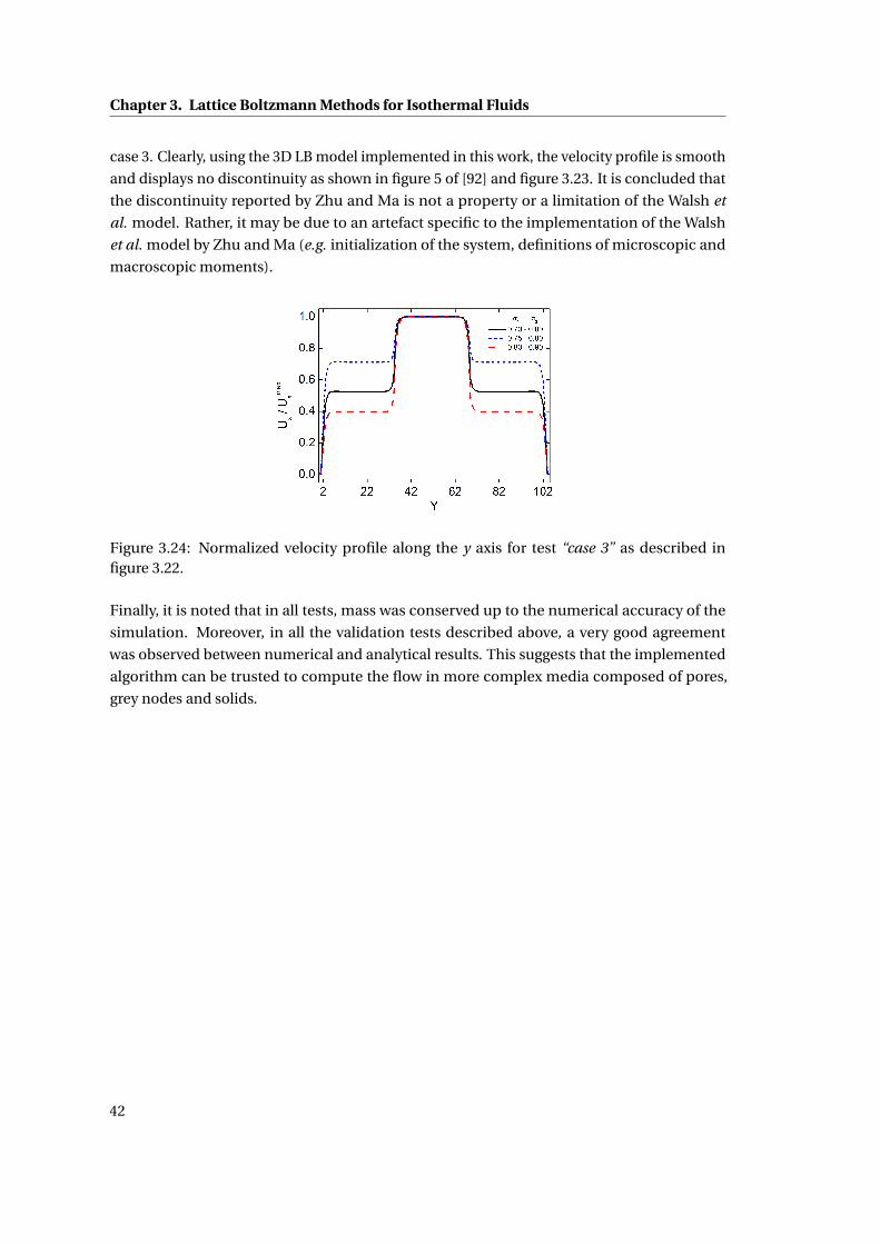
Chapter 3. Lattice Boltzmann Methods for Isothermal Fluids
case 3. Clearly, using the 3D LB model implemented in this work, the velocity profile is smooth
and displays no discontinuity as shown in figure 5 of [92] and figure 3.23. It is concluded that
the discontinuity reported by Zhu and Ma is not a property or a limitation of the Walsh et
al. model. Rather, it may be due to an artefact specific to the implementation of the Walsh
et al. model by Zhu and Ma (e.g. initialization of the system, definitions of microscopic and
macroscopic moments).
Figure 3.24: Normalized velocity profile along the y axis for test “case 3” as described infigure 3.22.
Finally, it is noted that in all tests, mass was conserved up to the numerical accuracy of the
simulation. Moreover, in all the validation tests described above, a very good agreement
was observed between numerical and analytical results. This suggests that the implemented
algorithm can be trusted to compute the flow in more complex media composed of pores,
grey nodes and solids.
42
4 Lattice Boltzmann Methods for non-Ideal Fluids
Contents
4.1 Standard methods . . . . . . . . . . . . . . . . . . . . . . . . . . . . . . . . . . 43
4.1.1 Overview . . . . . . . . . . . . . . . . . . . . . . . . . . . . . . . . . . . . . 43
4.1.2 Free energy approach for non-ideal fluids . . . . . . . . . . . . . . . . . 44
4.1.3 Wetting dynamics . . . . . . . . . . . . . . . . . . . . . . . . . . . . . . . . 46
4.1.4 Implementation . . . . . . . . . . . . . . . . . . . . . . . . . . . . . . . . . 47
4.1.5 Methods for modelling adsorption and desorption . . . . . . . . . . . . 48
4.1.6 Validation . . . . . . . . . . . . . . . . . . . . . . . . . . . . . . . . . . . . 48
4.2 Effective media methods for the transport and wetting properties . . . . . . 60
4.2.1 Overview . . . . . . . . . . . . . . . . . . . . . . . . . . . . . . . . . . . . . 60
4.2.2 Free energy approach for effective wetting properties . . . . . . . . . . 60
4.2.3 Implementation . . . . . . . . . . . . . . . . . . . . . . . . . . . . . . . . . 61
4.2.4 Methods for modelling adsorption and desorption . . . . . . . . . . . . 61
4.2.5 Validation . . . . . . . . . . . . . . . . . . . . . . . . . . . . . . . . . . . . 61
4.2.6 Application to a 2D characteristic microstructure . . . . . . . . . . . . . 65
4.2.7 Conclusions . . . . . . . . . . . . . . . . . . . . . . . . . . . . . . . . . . . 69
4.1 Standard methods
4.1.1 Overview
Numerical simulation of complex non-ideal fluids is rather challenging. In addition to the
theoretical framework that is required to describe the interactions between the multiple physi-
cal and chemical phases of the fluid, a numerical algorithm is needed to track the interfaces
between the phases. The latter part usually requires unrealistic computational costs. Notwith-
standing, lattice Boltzmann methods offer an implicit tracking of the interfaces. The creation,
43
Chapter 4. Lattice Boltzmann Methods for non-Ideal Fluids
movement and annihilation of interfaces are tracked automatically. Consequently, LB meth-
ods have been successful in simulating complex fluids for a wide variety of applications.
Three conceptually different algorithms have been developed to describe complex fluids:
Gunstensen et al. [94] developed a color-fluid algorithm particularly adapted for strong
phase separation, Shan and Chen [55] introduced an inter-particle potential that mimics
microscopic interactions, and Swift et al. [56] implemented a pressure tensor to incorporate a
free energy in the lattice Boltzmann algorithm. In the color-fluid model [94, 95], two fluids,
typically labelled red and blue, are introduced and phase separation is achieved by a forcing
particles to regions of the same colour. This model is particularly adapted for multi-fluid
applications with strong phase separation such as is the case for oil and water. The inter-
particle potential model of Shan and Chen [55] is based on the concept of interactions between
nearest-neighbours. In this model, the equilibrium velocity is modified in order to include an
interactive force that causes phase separation and creates surface tension. The main draw-
back is the dependency of both surface tension and equation of state on one single parameter.
Recently, this problem was addressed by Sbragaglia et al. [96] by extending the inter-particle
interactions to include the next-nearest-neighbours. While the two models described above
are based on phenomenological descriptions of the interface and dynamics, the free-energy
model of Swift et al. [56] uses equilibrium functions that can be defined more consistently,
based on thermodynamics. This makes it possible to implement an equation of state that
describes both liquid and gas phases, as well as their coexistence curve.
4.1.2 Free energy approach for non-ideal fluids
The equilibrium properties of a one-component non-ideal fluid with no solid surfaces can be
described by a Landau free energy functional [56, 97, 98]:
Ψ=∫
VdV
[ψ
(T,ρ
)+ χ
2
(∂αρ
)2]
. (4.1)
In this case,∫
V dV ρ is the total mass of the fluid, ψ(T,ρ
)the free energy density of the bulk
phase and T the temperature of the fluid. The second term of the RHS of equation 4.1 describes
the liquid – vapour interfaces and χ is a constant related to the surface tension between the
liquid and vapour phases.
This free energy can be incorporated in the lattice Boltzmann algorithm via the pressure tensor
[99, 100]:
Pαβ =[
p0 −χ(ρ∇2ρ+ 1
2
∣∣∇ρ∣∣2)]δαβ+χ∂αρ∂βρ (4.2)
where p0 is the equation of state of the fluid and the other terms, dependent on χ, describe
the liquid – vapour interfaces. The symbols ∂α, ∇ and ∇2 refer to the derivative with regards to
α, the gradient and the Laplacian operators, respectively. Summation over repeated indices is
44
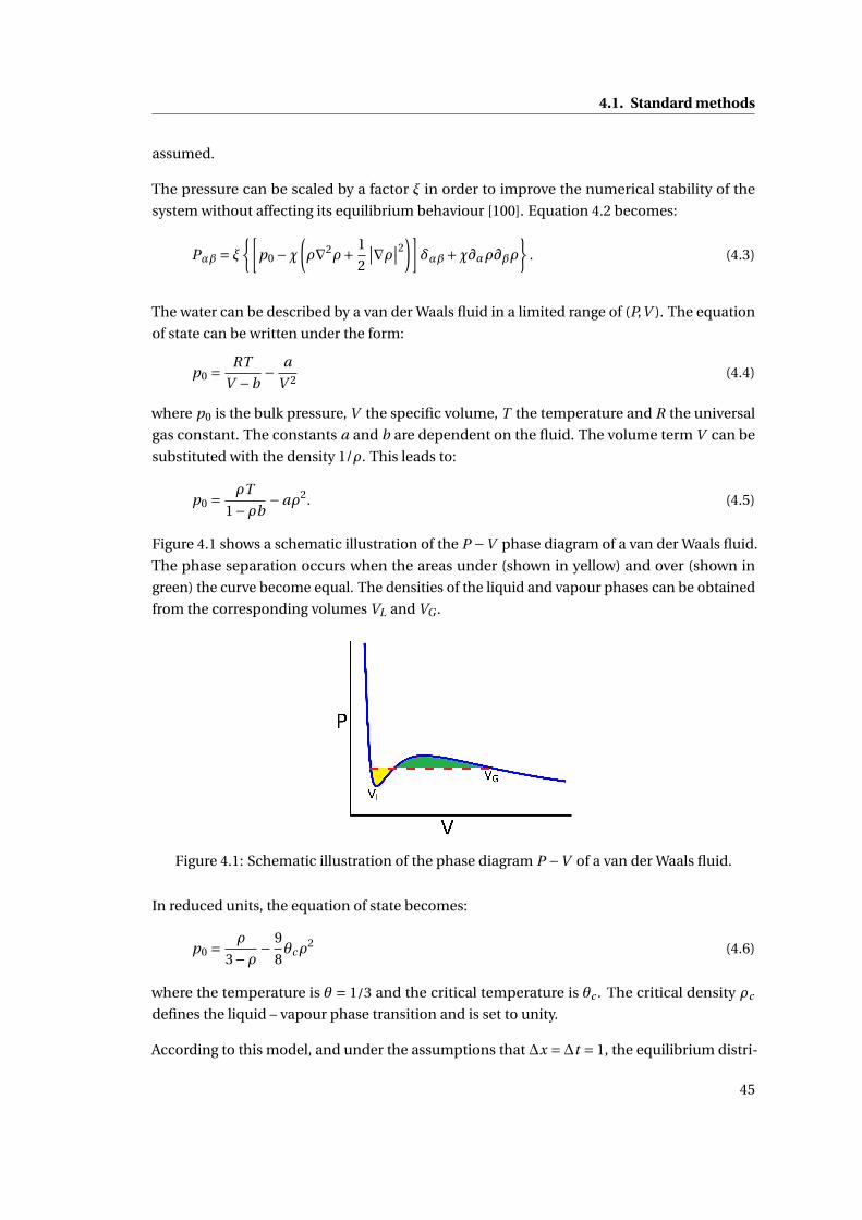
4.1. Standard methods
assumed.
The pressure can be scaled by a factor ξ in order to improve the numerical stability of the
system without affecting its equilibrium behaviour [100]. Equation 4.2 becomes:
Pαβ = ξ[
p0 −χ(ρ∇2ρ+ 1
2
∣∣∇ρ∣∣2)]δαβ+χ∂αρ∂βρ
. (4.3)
The water can be described by a van der Waals fluid in a limited range of (P,V ). The equation
of state can be written under the form:
p0 = RT
V −b− a
V 2 (4.4)
where p0 is the bulk pressure, V the specific volume, T the temperature and R the universal
gas constant. The constants a and b are dependent on the fluid. The volume term V can be
substituted with the density 1/ρ. This leads to:
p0 = ρT
1−ρb−aρ2. (4.5)
Figure 4.1 shows a schematic illustration of the P −V phase diagram of a van der Waals fluid.
The phase separation occurs when the areas under (shown in yellow) and over (shown in
green) the curve become equal. The densities of the liquid and vapour phases can be obtained
from the corresponding volumes VL and VG .
Figure 4.1: Schematic illustration of the phase diagram P −V of a van der Waals fluid.
In reduced units, the equation of state becomes:
p0 = ρ
3−ρ − 9
8θcρ
2 (4.6)
where the temperature is θ = 1/3 and the critical temperature is θc . The critical density ρc
defines the liquid – vapour phase transition and is set to unity.
According to this model, and under the assumptions that ∆x =∆t = 1, the equilibrium distri-
45
Chapter 4. Lattice Boltzmann Methods for non-Ideal Fluids
butions are [101]:
f eqi (r , t ) =ωi
[ρ (ei .u)+ 3
2ρ (ei .u)2 − 12ρ (u.u)+
32λ
[2(ei .u)
(ei .∇ρ)+ (ei .ei −1)
(u.∇ρ)] ]
+ωpi p0 −χ
(ωt
iρ∇2ρ+ ∑α=x;y ;z
ωααi ∂αρ∂αρ+ ∑α,β=x,y ;y,z;z,x
ωαβ
i ∂αρ∂βρ
) (4.7)
where the stationary equilibrium distribution function is chosen in order to conserve mass:
f eq1 (r , t ) = ρ (r , t )−
Q∑i=2
f eqi (r , t ) . (4.8)
The coefficientsωi are the lattice weights. The term involving the parameterλ ensures Galilean
invariance [102]:
λ=(τ− 1
2
)(1
3− d p0
dρ
). (4.9)
The last line of equation 4.7 gives the contribution of the pressure tensor. The coefficients
ωp,t ,αα,αβi are free adjustable parameters and can be found in [101].
It is worth noting that in addition to the macroscopic moments ρ and u, the equilibrium func-
tions require several derivative forms of the density. These operations make the computation
of the equilibrium functions very expensive, especially when compared to the operations
that are required to calculate the equilibrium functions of isothermal fluids (equation 3.11).
Additional information about the numerical algorithms that are used to calculate the gradients
in the bulk can be found in appendix D.
4.1.3 Wetting dynamics
The contact angle Θ quantifies the wettability of a solid surface by a liquid via the Young’s
equation [103]. Hence, the wetting dynamics can be incorporated in the lattice Boltzmann
simulations by creating a boundary condition that reproduces Young’s equation in equilibrium
[98]. The solid – liquid and solid – vapour surface tensions can be incorporated in the Landau
free energy functional by the addition of a surface term [98]. Cahn [104] assumed that the
fluid – solid interactions are short ranged so that they contribute to the total free energy of the
system with a surface integral:
Ψs =∫
SdSΦ
(ρs
). (4.10)
The total free energy becomes:
Ψ=∫
VdV
[ψ
(θ,ρ
)+ χ
2
(∂αρ
)2]+
∫S
dSΦ(ρs
)(4.11)
46
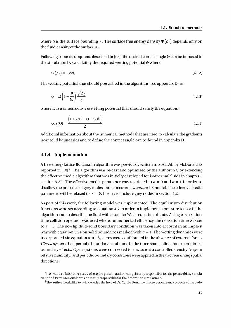
4.1. Standard methods
where S is the surface bounding V . The surface free energy density Φ(ρs
)depends only on
the fluid density at the surface ρs .
Following some assumptions described in [98], the desired contact angleΘ can be imposed in
the simulation by calculating the required wetting potential φ where
Φ(ρs
)=−φρs . (4.12)
The wetting potential that should prescribed in the algorithm (see appendix D) is:
φ=Ω(1− θ
θc
) √2χ
χ(4.13)
whereΩ is a dimension-less wetting potential that should satisfy the equation:
cos(Θ) =(1+Ω)
32 − (1−Ω)
32
)2
. (4.14)
Additional information about the numerical methods that are used to calculate the gradients
near solid boundaries and to define the contact angle can be found in appendix D.
4.1.4 Implementation
A free energy lattice Boltzmann algorithm was previously written in MATLAB by McDonald as
reported in [10]∗. The algorithm was re-cast and optimized by the author in C by extending
the effective media algorithm that was initially developed for isothermal fluids in chapter 3
section 3.2†. The effective media parameter was restricted to σ = 0 and σ = 1 in order to
disallow the presence of grey nodes and to recover a standard LB model. The effective media
parameter will be relaxed to σ= [0,1] so as to include grey nodes in section 4.2.
As part of this work, the following model was implemented. The equilibrium distribution
functions were set according to equation 4.7 in order to implement a pressure tensor in the
algorithm and to describe the fluid with a van der Waals equation of state. A single-relaxation-
time collision operator was used where, for numerical efficiency, the relaxation time was set
to τ = 1. The no-slip fluid-solid boundary condition was taken into account in an implicit
way with equation 3.24 on solid boundaries marked with σ= 1. The wetting dynamics were
incorporated via equation 4.10. Systems were equilibrated in the absence of external forces.
Closed systems had periodic boundary conditions in the three spatial directions to minimize
boundary effects. Open systems were connected to a source at a controlled density (vapour
relative humidity) and periodic boundary conditions were applied in the two remaining spatial
directions.
∗[10] was a collaborative study where the present author was primarily responsible for the permeability simula-tions and Peter McDonald was primarily responsible for the desorption simulations.
†The author would like to acknowledge the help of Dr. Cyrille Dunant with the performance aspects of the code.
47
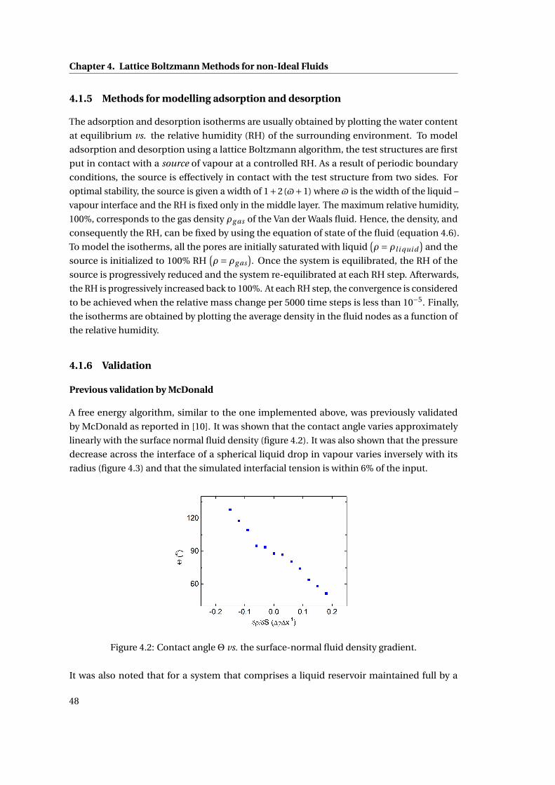
Chapter 4. Lattice Boltzmann Methods for non-Ideal Fluids
4.1.5 Methods for modelling adsorption and desorption
The adsorption and desorption isotherms are usually obtained by plotting the water content
at equilibrium vs. the relative humidity (RH) of the surrounding environment. To model
adsorption and desorption using a lattice Boltzmann algorithm, the test structures are first
put in contact with a source of vapour at a controlled RH. As a result of periodic boundary
conditions, the source is effectively in contact with the test structure from two sides. For
optimal stability, the source is given a width of 1+2($+1) where $ is the width of the liquid –
vapour interface and the RH is fixed only in the middle layer. The maximum relative humidity,
100%, corresponds to the gas density ρg as of the Van der Waals fluid. Hence, the density, and
consequently the RH, can be fixed by using the equation of state of the fluid (equation 4.6).
To model the isotherms, all the pores are initially saturated with liquid(ρ = ρl i qui d
)and the
source is initialized to 100% RH(ρ = ρg as
). Once the system is equilibrated, the RH of the
source is progressively reduced and the system re-equilibrated at each RH step. Afterwards,
the RH is progressively increased back to 100%. At each RH step, the convergence is considered
to be achieved when the relative mass change per 5000 time steps is less than 10−5. Finally,
the isotherms are obtained by plotting the average density in the fluid nodes as a function of
the relative humidity.
4.1.6 Validation
Previous validation by McDonald
A free energy algorithm, similar to the one implemented above, was previously validated
by McDonald as reported in [10]. It was shown that the contact angle varies approximately
linearly with the surface normal fluid density (figure 4.2). It was also shown that the pressure
decrease across the interface of a spherical liquid drop in vapour varies inversely with its
radius (figure 4.3) and that the simulated interfacial tension is within 6% of the input.
Figure 4.2: Contact angleΘ vs. the surface-normal fluid density gradient.
It was also noted that for a system that comprises a liquid reservoir maintained full by a
48
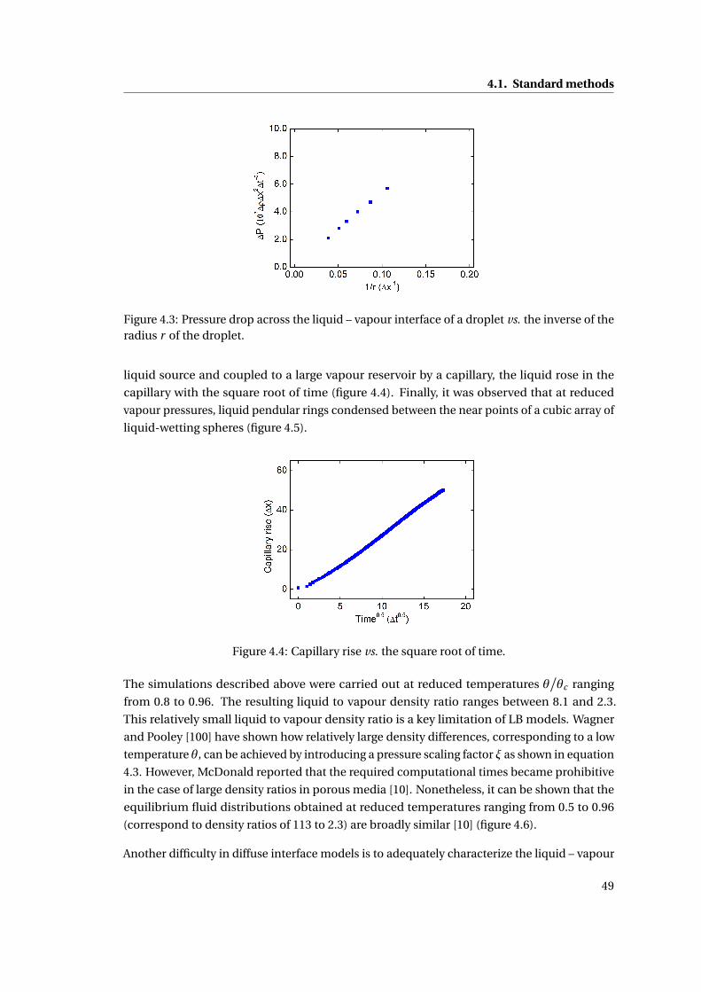
4.1. Standard methods
Figure 4.3: Pressure drop across the liquid – vapour interface of a droplet vs. the inverse of theradius r of the droplet.
liquid source and coupled to a large vapour reservoir by a capillary, the liquid rose in the
capillary with the square root of time (figure 4.4). Finally, it was observed that at reduced
vapour pressures, liquid pendular rings condensed between the near points of a cubic array of
liquid-wetting spheres (figure 4.5).
Figure 4.4: Capillary rise vs. the square root of time.
The simulations described above were carried out at reduced temperatures θ/θc ranging
from 0.8 to 0.96. The resulting liquid to vapour density ratio ranges between 8.1 and 2.3.
This relatively small liquid to vapour density ratio is a key limitation of LB models. Wagner
and Pooley [100] have shown how relatively large density differences, corresponding to a low
temperature θ, can be achieved by introducing a pressure scaling factor ξ as shown in equation
4.3. However, McDonald reported that the required computational times became prohibitive
in the case of large density ratios in porous media [10]. Nonetheless, it can be shown that the
equilibrium fluid distributions obtained at reduced temperatures ranging from 0.5 to 0.96
(correspond to density ratios of 113 to 2.3) are broadly similar [10] (figure 4.6).
Another difficulty in diffuse interface models is to adequately characterize the liquid – vapour
49
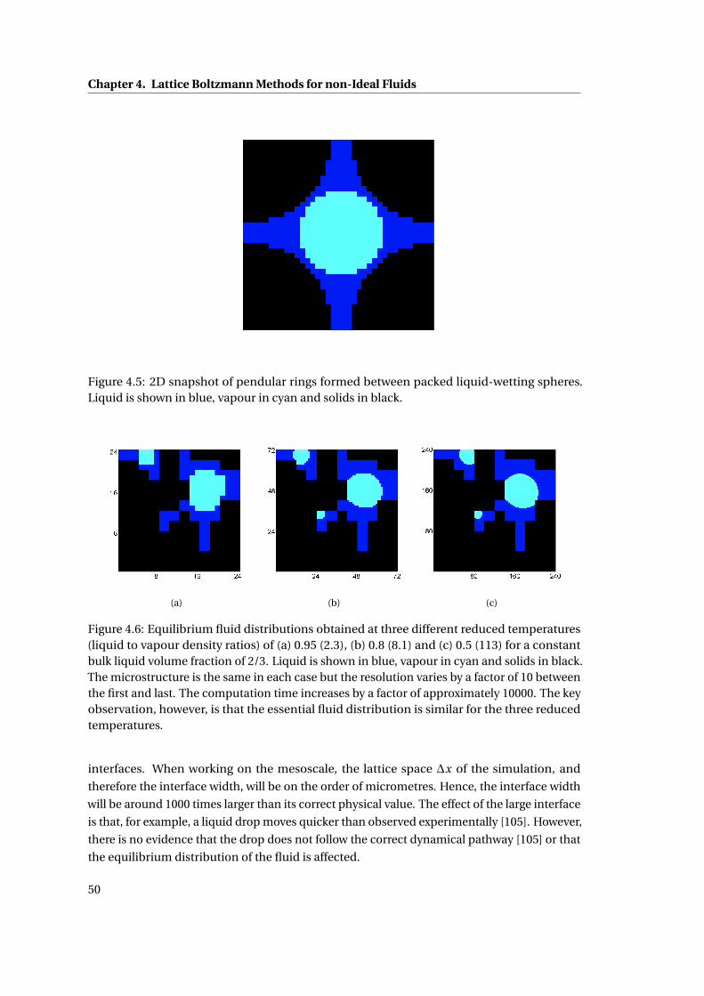
Chapter 4. Lattice Boltzmann Methods for non-Ideal Fluids
Figure 4.5: 2D snapshot of pendular rings formed between packed liquid-wetting spheres.Liquid is shown in blue, vapour in cyan and solids in black.
(a) (b) (c)
Figure 4.6: Equilibrium fluid distributions obtained at three different reduced temperatures(liquid to vapour density ratios) of (a) 0.95 (2.3), (b) 0.8 (8.1) and (c) 0.5 (113) for a constantbulk liquid volume fraction of 2/3. Liquid is shown in blue, vapour in cyan and solids in black.The microstructure is the same in each case but the resolution varies by a factor of 10 betweenthe first and last. The computation time increases by a factor of approximately 10000. The keyobservation, however, is that the essential fluid distribution is similar for the three reducedtemperatures.
interfaces. When working on the mesoscale, the lattice space ∆x of the simulation, and
therefore the interface width, will be on the order of micrometres. Hence, the interface width
will be around 1000 times larger than its correct physical value. The effect of the large interface
is that, for example, a liquid drop moves quicker than observed experimentally [105]. However,
there is no evidence that the drop does not follow the correct dynamical pathway [105] or that
the equilibrium distribution of the fluid is affected.
50
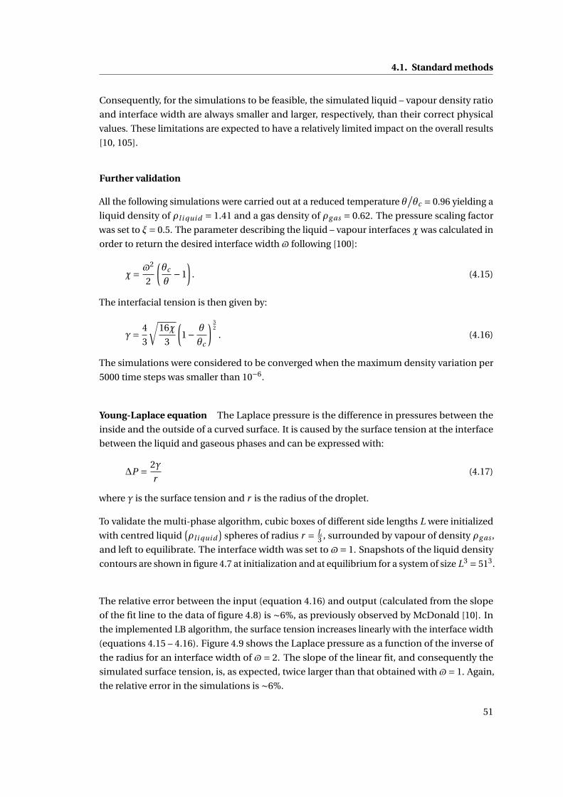
4.1. Standard methods
Consequently, for the simulations to be feasible, the simulated liquid – vapour density ratio
and interface width are always smaller and larger, respectively, than their correct physical
values. These limitations are expected to have a relatively limited impact on the overall results
[10, 105].
Further validation
All the following simulations were carried out at a reduced temperature θ/θc = 0.96 yielding a
liquid density of ρl i qui d = 1.41 and a gas density of ρg as = 0.62. The pressure scaling factor
was set to ξ= 0.5. The parameter describing the liquid – vapour interfaces χ was calculated in
order to return the desired interface width $ following [100]:
χ= $2
2
(θc
θ−1
). (4.15)
The interfacial tension is then given by:
γ= 4
3
√16χ
3
(1− θ
θc
) 32
. (4.16)
The simulations were considered to be converged when the maximum density variation per
5000 time steps was smaller than 10−6.
Young-Laplace equation The Laplace pressure is the difference in pressures between the
inside and the outside of a curved surface. It is caused by the surface tension at the interface
between the liquid and gaseous phases and can be expressed with:
∆P = 2γ
r(4.17)
where γ is the surface tension and r is the radius of the droplet.
To validate the multi-phase algorithm, cubic boxes of different side lengths L were initialized
with centred liquid(ρl i qui d
)spheres of radius r = L
3 , surrounded by vapour of density ρg as ,
and left to equilibrate. The interface width was set to $= 1. Snapshots of the liquid density
contours are shown in figure 4.7 at initialization and at equilibrium for a system of size L3 = 513.
The relative error between the input (equation 4.16) and output (calculated from the slope
of the fit line to the data of figure 4.8) is ∼6%, as previously observed by McDonald [10]. In
the implemented LB algorithm, the surface tension increases linearly with the interface width
(equations 4.15 – 4.16). Figure 4.9 shows the Laplace pressure as a function of the inverse of
the radius for an interface width of $= 2. The slope of the linear fit, and consequently the
simulated surface tension, is, as expected, twice larger than that obtained with $= 1. Again,
the relative error in the simulations is ∼6%.
51
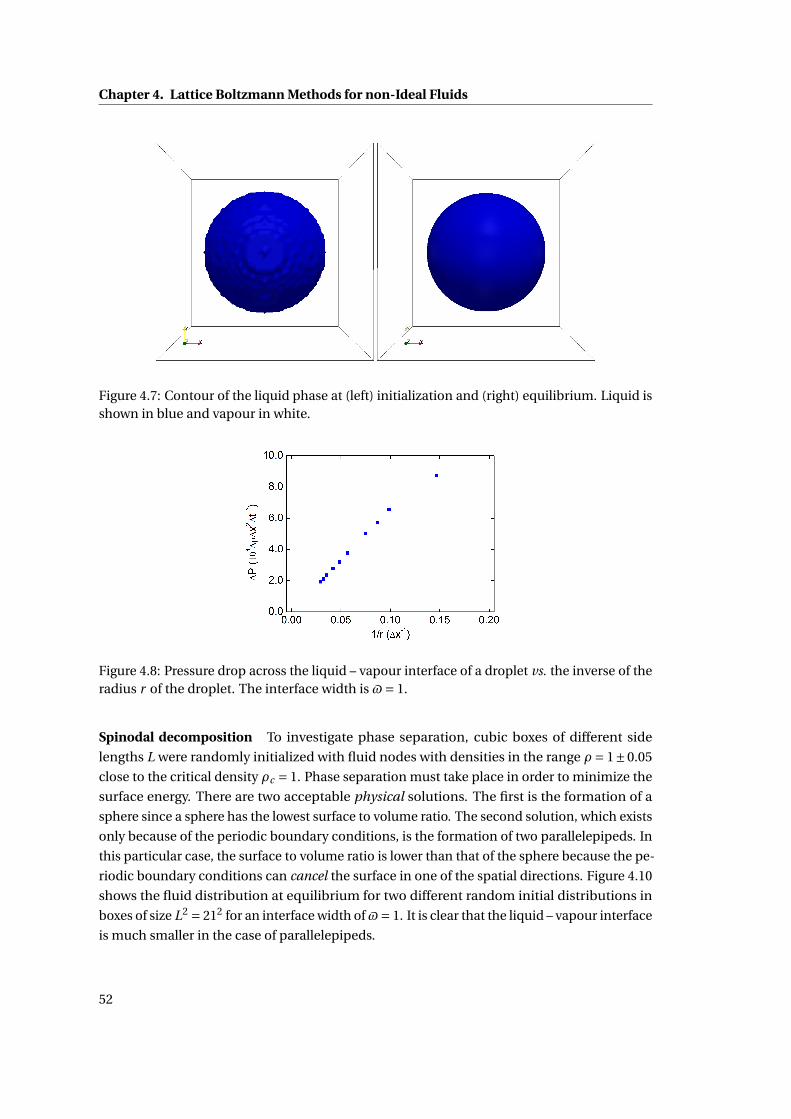
Chapter 4. Lattice Boltzmann Methods for non-Ideal Fluids
Figure 4.7: Contour of the liquid phase at (left) initialization and (right) equilibrium. Liquid isshown in blue and vapour in white.
Figure 4.8: Pressure drop across the liquid – vapour interface of a droplet vs. the inverse of theradius r of the droplet. The interface width is $= 1.
Spinodal decomposition To investigate phase separation, cubic boxes of different side
lengths L were randomly initialized with fluid nodes with densities in the range ρ = 1±0.05
close to the critical density ρc = 1. Phase separation must take place in order to minimize the
surface energy. There are two acceptable physical solutions. The first is the formation of a
sphere since a sphere has the lowest surface to volume ratio. The second solution, which exists
only because of the periodic boundary conditions, is the formation of two parallelepipeds. In
this particular case, the surface to volume ratio is lower than that of the sphere because the pe-
riodic boundary conditions can cancel the surface in one of the spatial directions. Figure 4.10
shows the fluid distribution at equilibrium for two different random initial distributions in
boxes of size L2 = 212 for an interface width of$= 1. It is clear that the liquid – vapour interface
is much smaller in the case of parallelepipeds.
52
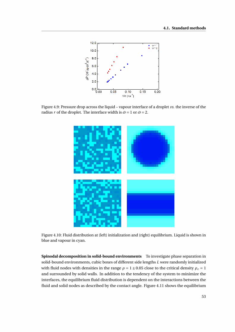
4.1. Standard methods
Figure 4.9: Pressure drop across the liquid – vapour interface of a droplet vs. the inverse of theradius r of the droplet. The interface width is $= 1 or $= 2.
Figure 4.10: Fluid distribution at (left) initialization and (right) equilibrium. Liquid is shown inblue and vapour in cyan.
Spinodal decomposition in solid-bound environments To investigate phase separation in
solid-bound environments, cubic boxes of different side lengths L were randomly initialized
with fluid nodes with densities in the range ρ = 1±0.05 close to the critical density ρc = 1
and surrounded by solid walls. In addition to the tendency of the system to minimize the
interfaces, the equilibrium fluid distribution is dependent on the interactions between the
fluid and solid nodes as described by the contact angle. Figure 4.11 shows the equilibrium
53
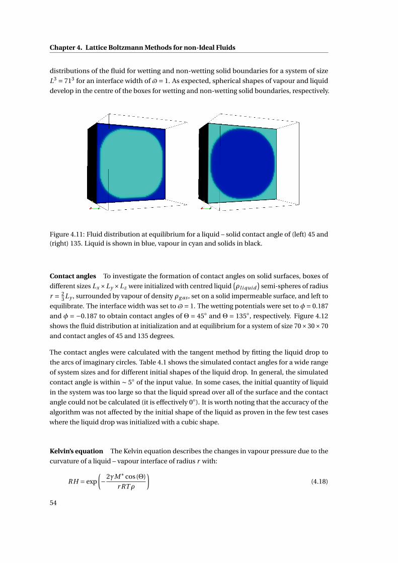
Chapter 4. Lattice Boltzmann Methods for non-Ideal Fluids
distributions of the fluid for wetting and non-wetting solid boundaries for a system of size
L3 = 713 for an interface width of $= 1. As expected, spherical shapes of vapour and liquid
develop in the centre of the boxes for wetting and non-wetting solid boundaries, respectively.
Figure 4.11: Fluid distribution at equilibrium for a liquid – solid contact angle of (left) 45 and(right) 135. Liquid is shown in blue, vapour in cyan and solids in black.
Contact angles To investigate the formation of contact angles on solid surfaces, boxes of
different sizes Lx ×Ly ×Lz were initialized with centred liquid(ρl i qui d
)semi-spheres of radius
r = 23 Ly , surrounded by vapour of density ρg as , set on a solid impermeable surface, and left to
equilibrate. The interface width was set to $= 1. The wetting potentials were set to φ= 0.187
and φ = −0.187 to obtain contact angles of Θ = 45 and Θ = 135, respectively. Figure 4.12
shows the fluid distribution at initialization and at equilibrium for a system of size 70×30×70
and contact angles of 45 and 135 degrees.
The contact angles were calculated with the tangent method by fitting the liquid drop to
the arcs of imaginary circles. Table 4.1 shows the simulated contact angles for a wide range
of system sizes and for different initial shapes of the liquid drop. In general, the simulated
contact angle is within ∼ 5 of the input value. In some cases, the initial quantity of liquid
in the system was too large so that the liquid spread over all of the surface and the contact
angle could not be calculated (it is effectively 0). It is worth noting that the accuracy of the
algorithm was not affected by the initial shape of the liquid as proven in the few test cases
where the liquid drop was initialized with a cubic shape.
Kelvin’s equation The Kelvin equation describes the changes in vapour pressure due to the
curvature of a liquid – vapour interface of radius r with:
RH = exp
(−2γM∗ cos(Θ)
r RTρ
)(4.18)
54
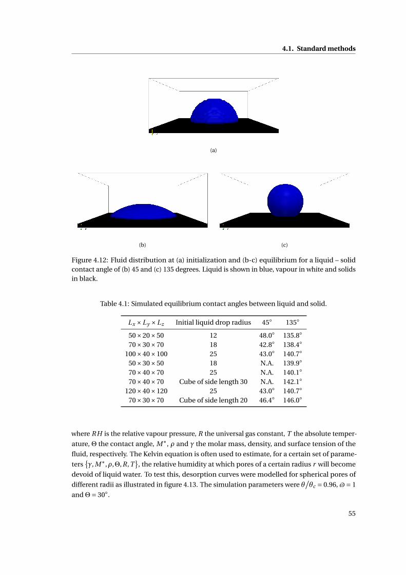
4.1. Standard methods
(a)
(b) (c)
Figure 4.12: Fluid distribution at (a) initialization and (b-c) equilibrium for a liquid – solidcontact angle of (b) 45 and (c) 135 degrees. Liquid is shown in blue, vapour in white and solidsin black.
Table 4.1: Simulated equilibrium contact angles between liquid and solid.
Lx ×Ly ×Lz Initial liquid drop radius 45 135
50×20×50 12 48.0 135.8
70×30×70 18 42.8 138.4
100×40×100 25 43.0 140.7
50×30×50 18 N.A. 139.9
70×40×70 25 N.A. 140.1
70×40×70 Cube of side length 30 N.A. 142.1
120×40×120 25 43.0 140.7
70×30×70 Cube of side length 20 46.4 146.0
where RH is the relative vapour pressure, R the universal gas constant, T the absolute temper-
ature, Θ the contact angle, M∗, ρ and γ the molar mass, density, and surface tension of the
fluid, respectively. The Kelvin equation is often used to estimate, for a certain set of parame-
tersγ, M∗,ρ,Θ,R,T
, the relative humidity at which pores of a certain radius r will become
devoid of liquid water. To test this, desorption curves were modelled for spherical pores of
different radii as illustrated in figure 4.13. The simulation parameters were θ/θc = 0.96, $= 1
andΘ= 30.
55
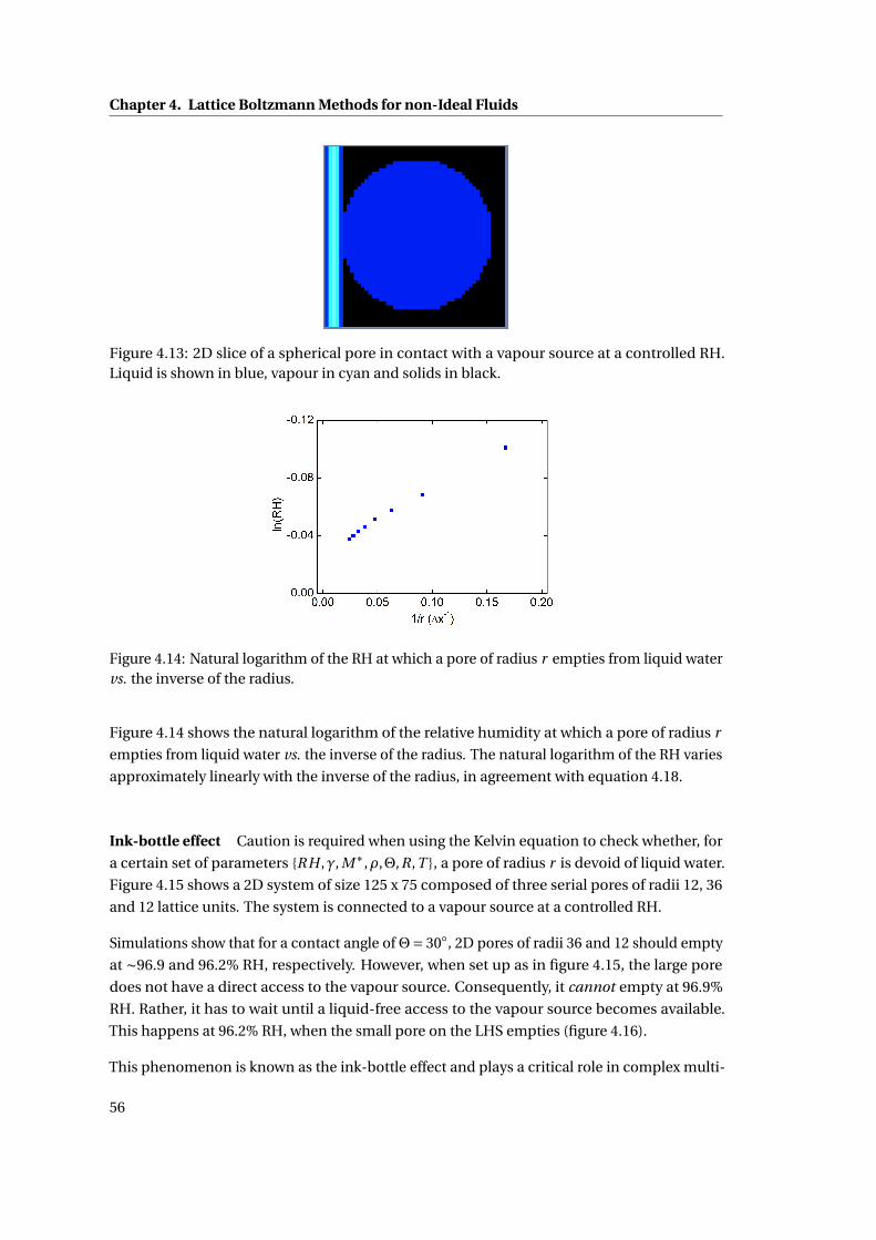
Chapter 4. Lattice Boltzmann Methods for non-Ideal Fluids
Figure 4.13: 2D slice of a spherical pore in contact with a vapour source at a controlled RH.Liquid is shown in blue, vapour in cyan and solids in black.
Figure 4.14: Natural logarithm of the RH at which a pore of radius r empties from liquid watervs. the inverse of the radius.
Figure 4.14 shows the natural logarithm of the relative humidity at which a pore of radius r
empties from liquid water vs. the inverse of the radius. The natural logarithm of the RH varies
approximately linearly with the inverse of the radius, in agreement with equation 4.18.
Ink-bottle effect Caution is required when using the Kelvin equation to check whether, for
a certain set of parameters RH ,γ, M∗,ρ,Θ,R,T , a pore of radius r is devoid of liquid water.
Figure 4.15 shows a 2D system of size 125 x 75 composed of three serial pores of radii 12, 36
and 12 lattice units. The system is connected to a vapour source at a controlled RH.
Simulations show that for a contact angle ofΘ= 30, 2D pores of radii 36 and 12 should empty
at ∼96.9 and 96.2% RH, respectively. However, when set up as in figure 4.15, the large pore
does not have a direct access to the vapour source. Consequently, it cannot empty at 96.9%
RH. Rather, it has to wait until a liquid-free access to the vapour source becomes available.
This happens at 96.2% RH, when the small pore on the LHS empties (figure 4.16).
This phenomenon is known as the ink-bottle effect and plays a critical role in complex multi-
56
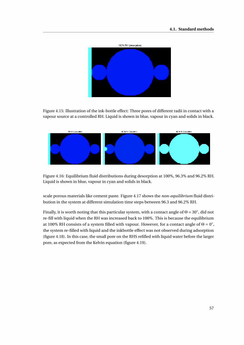
4.1. Standard methods
Figure 4.15: Illustration of the ink-bottle effect: Three pores of different radii in contact with avapour source at a controlled RH. Liquid is shown in blue, vapour in cyan and solids in black.
Figure 4.16: Equilibrium fluid distributions during desorption at 100%, 96.3% and 96.2% RH.Liquid is shown in blue, vapour in cyan and solids in black.
scale porous materials like cement paste. Figure 4.17 shows the non-equilibrium fluid distri-
bution in the system at different simulation time steps between 96.3 and 96.2% RH.
Finally, it is worth noting that this particular system, with a contact angle ofΘ= 30, did not
re-fill with liquid when the RH was increased back to 100%. This is because the equilibrium
at 100% RH consists of a system filled with vapour. However, for a contact angle of Θ = 0,
the system re-filled with liquid and the inkbottle effect was not observed during adsorption
(figure 4.18). In this case, the small pore on the RHS refilled with liquid water before the larger
pore, as expected from the Kelvin equation (figure 4.19).
57
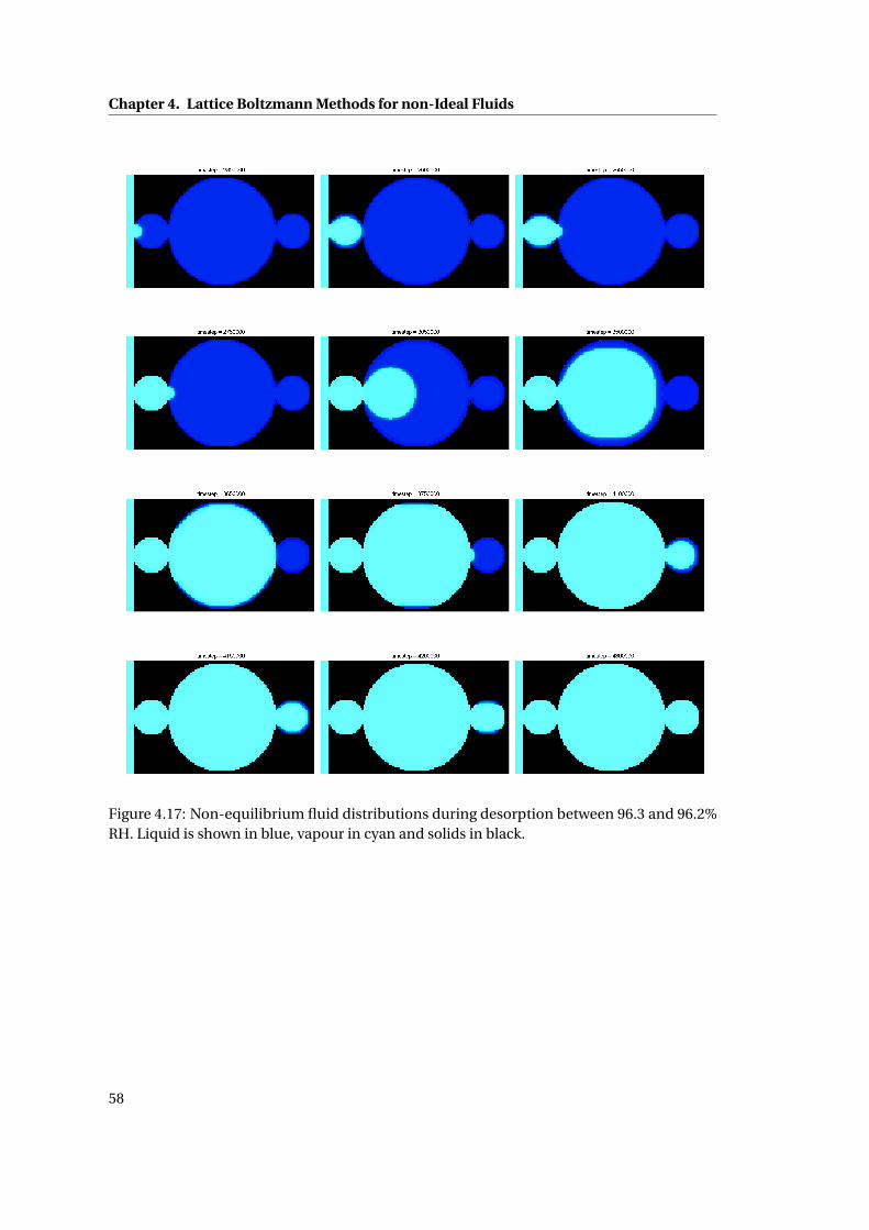
Chapter 4. Lattice Boltzmann Methods for non-Ideal Fluids
Figure 4.17: Non-equilibrium fluid distributions during desorption between 96.3 and 96.2%RH. Liquid is shown in blue, vapour in cyan and solids in black.
58
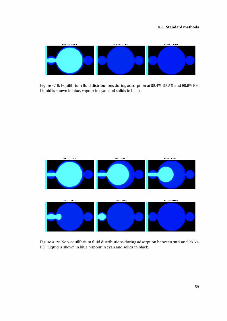
4.1. Standard methods
Figure 4.18: Equilibrium fluid distributions during adsorption at 98.4%, 98.5% and 98.6% RH.Liquid is shown in blue, vapour in cyan and solids in black.
Figure 4.19: Non-equilibrium fluid distributions during adsorption between 98.5 and 98.6%RH. Liquid is shown in blue, vapour in cyan and solids in black.
59
Chapter 4. Lattice Boltzmann Methods for non-Ideal Fluids
4.2 Effective media methods for the transport and wetting proper-
ties
4.2.1 Overview
The methodology introduced in chapter 3 section 3.2 allows the introduction of grey nodes
with effective transport properties. This allows, as will be shown in chapter 5 section 5.2 to
overcome the difficulty of modelling the flow in microstructures where the porosity spans
several length scales. The approach introduced in section 4.1 makes it possible to describe
the fluid with an equation of state. This is necessary, as will be shown in chapter 6, to study
desorption and adsorption of water in unsaturated cement paste model microstructures. The
question that arises is whether the two methods can be combined to tackle both problems
simultaneously, that is, whether it is possible to define grey nodes with effective transport and
wetting properties.
In this section, the novel step is made of interpreting the effective wetting within a free energy
framework. This is done without rigorous mathematical derivation and perhaps, such a
derivation is not possible. However, this approach has great merit as will be shown below
and in chapter 6. The method combines two independent parameters, the effective media
parameter σg r e y that describes the intrinsic permeability of the grey nodes, with the internal
wetting parameter φg r e y that describes the wetting behaviour of the grey nodes. Having two
independent parameters enables the model to be tuned so as to reasonably characterize both
permeability and adsorption and desorption isotherms. Neither of the previous models could
do this alone. In particular, it will be shown that the sorption isotherms are independent of
the permeability (as long as the grey nodes are permeable). It will also be shown that two-step
isotherms can be obtained for media composed of pores, grey nodes, and solids.
4.2.2 Free energy approach for effective wetting properties
The free energy functional was previously defined for fluid nodes (σ= 0) in bulk (equation
4.1) and near solid surfaces (equation 4.10). The presence of grey nodes (0 <σ< 1) creates an
additional class of bulk nodes. Thus, the volume term of equation 4.1, originally including only
the fluid nodes V ⊂ σ= 0, should henceforth include the grey nodes so that: V ⊂ 0 ≤σ< 1.
Moreover, the presence of grey nodes creates additional classes of surfaces. Accordingly,
equation 4.10,∫
S dSΦ(ρs
), is extended to:
∑ς
∫Sς
dSςΦς(ρς
)(4.19)
60
4.2. Effective media methods for the transport and wetting properties
where the sum is over the classes of surfaces ς. In the simplest case, the surfaces are:
ς⊂
fluid over solid nodes
fluid over grey nodes
grey over solid nodes
. (4.20)
Lastly, it is assumed that the grey nodes contribute an effective energy to the total free energy
through their internal wetting via:∫Vg r e y
dVg r e yΦg r e y(ρg r e y
)(4.21)
whereΦg r e y(ρg r e y
)characterizes the internal wetting of the grey nodes. The total free energy
therefore becomes:
Ψ=∫
VdV
[ψ
(θ,ρ
)+ χ
2
(∂αρ
)2]+∑
ς
∫Sς
dSςΦς(ρς
)+∫Vg r e y
dVg r e yΦg r e y(ρg r e y
). (4.22)
The effective media parameter σg r e y defines the grey nodes in terms of intrinsic transport
properties andΦg r e y defines them in terms of internal wetting. The characteristic features of
this effective free energy will be demonstrated in the next sections.
4.2.3 Implementation
The effective media free energy algorithm was implemented as an extension to the standard
free energy algorithm as previously discussed in section 4.1.4.
4.2.4 Methods for modelling adsorption and desorption
The isotherms are modelled in a similar fashion to that discussed in section 4.1.5. However, in
addition to the pores, the grey nodes are initialized with liquid water and are included in the
calculation of the average mass of adsorbed fluid.
4.2.5 Validation
For the validation of the effective media algorithm for non-ideal fluids, the interactions
between fluid and grey nodes, between grey and solid nodes, and inside grey nodes were
analysed. All the following simulations were carried out at a reduced temperature θ/θc = 0.96
yielding a liquid density of ρl i qui d = 1.41 and a gas density of ρg as = 0.62. The pressure
scaling factor was set to ξ= 0.5. The parameter describing the liquid – vapour interfaces χ was
calculated using equation 4.15 in order to return an interface width $= 1.
61
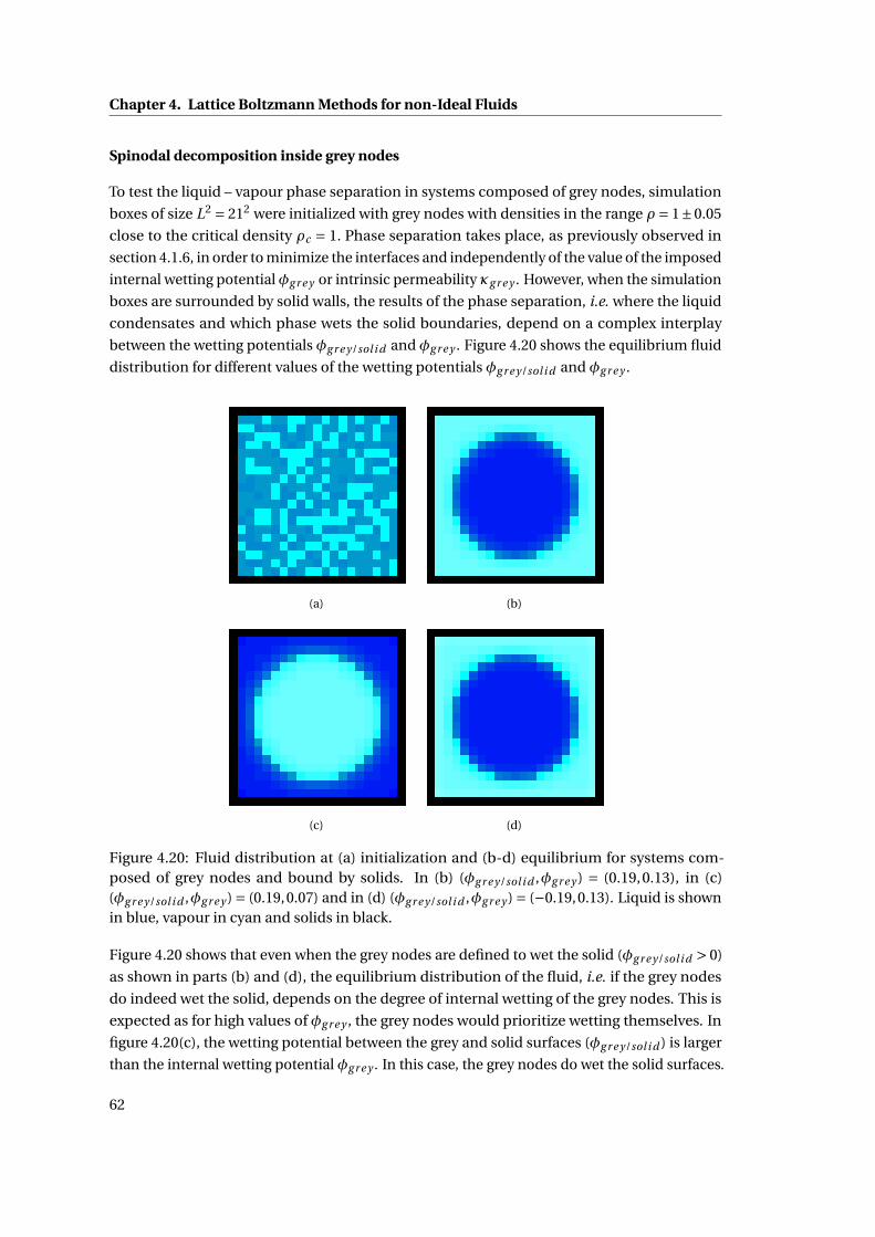
Chapter 4. Lattice Boltzmann Methods for non-Ideal Fluids
Spinodal decomposition inside grey nodes
To test the liquid – vapour phase separation in systems composed of grey nodes, simulation
boxes of size L2 = 212 were initialized with grey nodes with densities in the range ρ = 1±0.05
close to the critical density ρc = 1. Phase separation takes place, as previously observed in
section 4.1.6, in order to minimize the interfaces and independently of the value of the imposed
internal wetting potentialφg r e y or intrinsic permeability κg r e y . However, when the simulation
boxes are surrounded by solid walls, the results of the phase separation, i.e. where the liquid
condensates and which phase wets the solid boundaries, depend on a complex interplay
between the wetting potentials φg r e y/sol i d and φg r e y . Figure 4.20 shows the equilibrium fluid
distribution for different values of the wetting potentials φg r e y/sol i d and φg r e y .
(a) (b)
(c) (d)
Figure 4.20: Fluid distribution at (a) initialization and (b-d) equilibrium for systems com-posed of grey nodes and bound by solids. In (b) (φg r e y/sol i d ,φg r e y ) = (0.19,0.13), in (c)(φg r e y/sol i d ,φg r e y ) = (0.19,0.07) and in (d) (φg r e y/sol i d ,φg r e y ) = (−0.19,0.13). Liquid is shownin blue, vapour in cyan and solids in black.
Figure 4.20 shows that even when the grey nodes are defined to wet the solid (φg r e y/sol i d > 0)
as shown in parts (b) and (d), the equilibrium distribution of the fluid, i.e. if the grey nodes
do indeed wet the solid, depends on the degree of internal wetting of the grey nodes. This is
expected as for high values of φg r e y , the grey nodes would prioritize wetting themselves. In
figure 4.20(c), the wetting potential between the grey and solid surfaces (φg r e y/sol i d ) is larger
than the internal wetting potential φg r e y . In this case, the grey nodes do wet the solid surfaces.
62
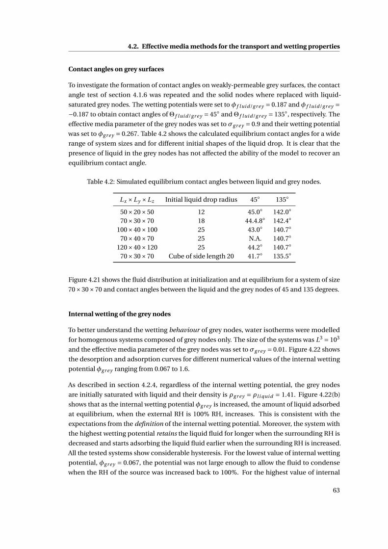
4.2. Effective media methods for the transport and wetting properties
Contact angles on grey surfaces
To investigate the formation of contact angles on weakly-permeable grey surfaces, the contact
angle test of section 4.1.6 was repeated and the solid nodes where replaced with liquid-
saturated grey nodes. The wetting potentials were set to φ f lui d/g r e y = 0.187 and φ f lui d/g r e y =−0.187 to obtain contact angles ofΘ f lui d/g r e y = 45 andΘ f lui d/g r e y = 135, respectively. The
effective media parameter of the grey nodes was set to σg r e y = 0.9 and their wetting potential
was set to φg r e y = 0.267. Table 4.2 shows the calculated equilibrium contact angles for a wide
range of system sizes and for different initial shapes of the liquid drop. It is clear that the
presence of liquid in the grey nodes has not affected the ability of the model to recover an
equilibrium contact angle.
Table 4.2: Simulated equilibrium contact angles between liquid and grey nodes.
Lx ×Ly ×Lz Initial liquid drop radius 45 135
50×20×50 12 45.0 142.0
70×30×70 18 44.4.8 142.4
100×40×100 25 43.0 140.7
70×40×70 25 N.A. 140.7
120×40×120 25 44.2 140.7
70×30×70 Cube of side length 20 41.7 135.5
Figure 4.21 shows the fluid distribution at initialization and at equilibrium for a system of size
70×30×70 and contact angles between the liquid and the grey nodes of 45 and 135 degrees.
Internal wetting of the grey nodes
To better understand the wetting behaviour of grey nodes, water isotherms were modelled
for homogenous systems composed of grey nodes only. The size of the systems was L3 = 103
and the effective media parameter of the grey nodes was set to σg r e y = 0.01. Figure 4.22 shows
the desorption and adsorption curves for different numerical values of the internal wetting
potential φg r e y ranging from 0.067 to 1.6.
As described in section 4.2.4, regardless of the internal wetting potential, the grey nodes
are initially saturated with liquid and their density is ρg r e y = ρl i qui d = 1.41. Figure 4.22(b)
shows that as the internal wetting potential φg r e y is increased, the amount of liquid adsorbed
at equilibrium, when the external RH is 100% RH, increases. This is consistent with the
expectations from the definition of the internal wetting potential. Moreover, the system with
the highest wetting potential retains the liquid fluid for longer when the surrounding RH is
decreased and starts adsorbing the liquid fluid earlier when the surrounding RH is increased.
All the tested systems show considerable hysteresis. For the lowest value of internal wetting
potential, φg r e y = 0.067, the potential was not large enough to allow the fluid to condense
when the RH of the source was increased back to 100%. For the highest value of internal
63
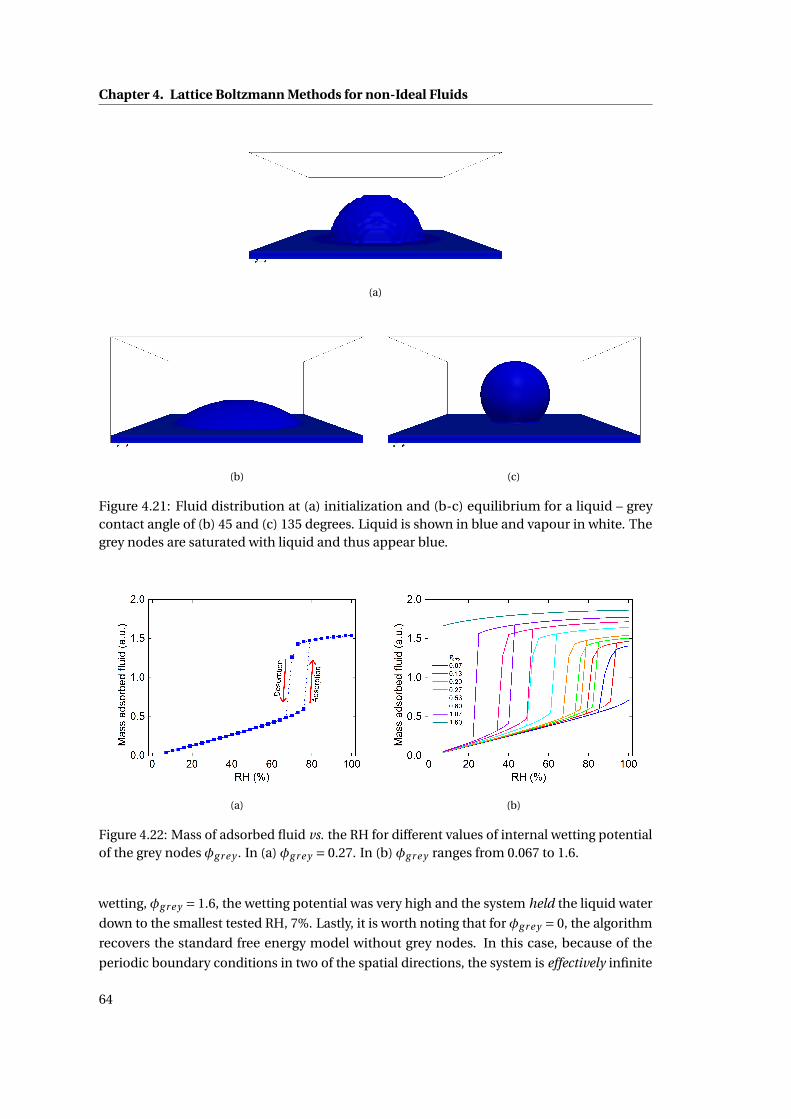
Chapter 4. Lattice Boltzmann Methods for non-Ideal Fluids
(a)
(b) (c)
Figure 4.21: Fluid distribution at (a) initialization and (b-c) equilibrium for a liquid – greycontact angle of (b) 45 and (c) 135 degrees. Liquid is shown in blue and vapour in white. Thegrey nodes are saturated with liquid and thus appear blue.
(a) (b)
Figure 4.22: Mass of adsorbed fluid vs. the RH for different values of internal wetting potentialof the grey nodes φg r e y . In (a) φg r e y = 0.27. In (b) φg r e y ranges from 0.067 to 1.6.
wetting, φg r e y = 1.6, the wetting potential was very high and the system held the liquid water
down to the smallest tested RH, 7%. Lastly, it is worth noting that for φg r e y = 0, the algorithm
recovers the standard free energy model without grey nodes. In this case, because of the
periodic boundary conditions in two of the spatial directions, the system is effectively infinite
64
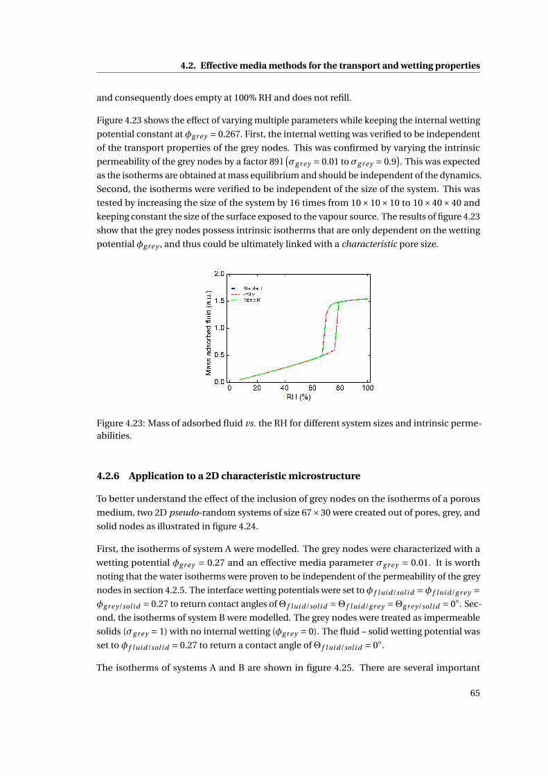
4.2. Effective media methods for the transport and wetting properties
and consequently does empty at 100% RH and does not refill.
Figure 4.23 shows the effect of varying multiple parameters while keeping the internal wetting
potential constant at φg r e y = 0.267. First, the internal wetting was verified to be independent
of the transport properties of the grey nodes. This was confirmed by varying the intrinsic
permeability of the grey nodes by a factor 891(σg r e y = 0.01 toσg r e y = 0.9
). This was expected
as the isotherms are obtained at mass equilibrium and should be independent of the dynamics.
Second, the isotherms were verified to be independent of the size of the system. This was
tested by increasing the size of the system by 16 times from 10×10×10 to 10×40×40 and
keeping constant the size of the surface exposed to the vapour source. The results of figure 4.23
show that the grey nodes possess intrinsic isotherms that are only dependent on the wetting
potential φg r e y , and thus could be ultimately linked with a characteristic pore size.
Figure 4.23: Mass of adsorbed fluid vs. the RH for different system sizes and intrinsic perme-abilities.
4.2.6 Application to a 2D characteristic microstructure
To better understand the effect of the inclusion of grey nodes on the isotherms of a porous
medium, two 2D pseudo-random systems of size 67×30 were created out of pores, grey, and
solid nodes as illustrated in figure 4.24.
First, the isotherms of system A were modelled. The grey nodes were characterized with a
wetting potential φg r e y = 0.27 and an effective media parameter σg r e y = 0.01. It is worth
noting that the water isotherms were proven to be independent of the permeability of the grey
nodes in section 4.2.5. The interface wetting potentials were set to φ f lui d/sol i d =φ f lui d/g r e y =φg r e y/sol i d = 0.27 to return contact angles ofΘ f lui d/sol i d =Θ f lui d/g r e y =Θg r e y/sol i d = 0. Sec-
ond, the isotherms of system B were modelled. The grey nodes were treated as impermeable
solids (σg r e y = 1) with no internal wetting (φg r e y = 0). The fluid – solid wetting potential was
set to φ f lui d/sol i d = 0.27 to return a contact angle ofΘ f lui d/sol i d = 0.
The isotherms of systems A and B are shown in figure 4.25. There are several important
65
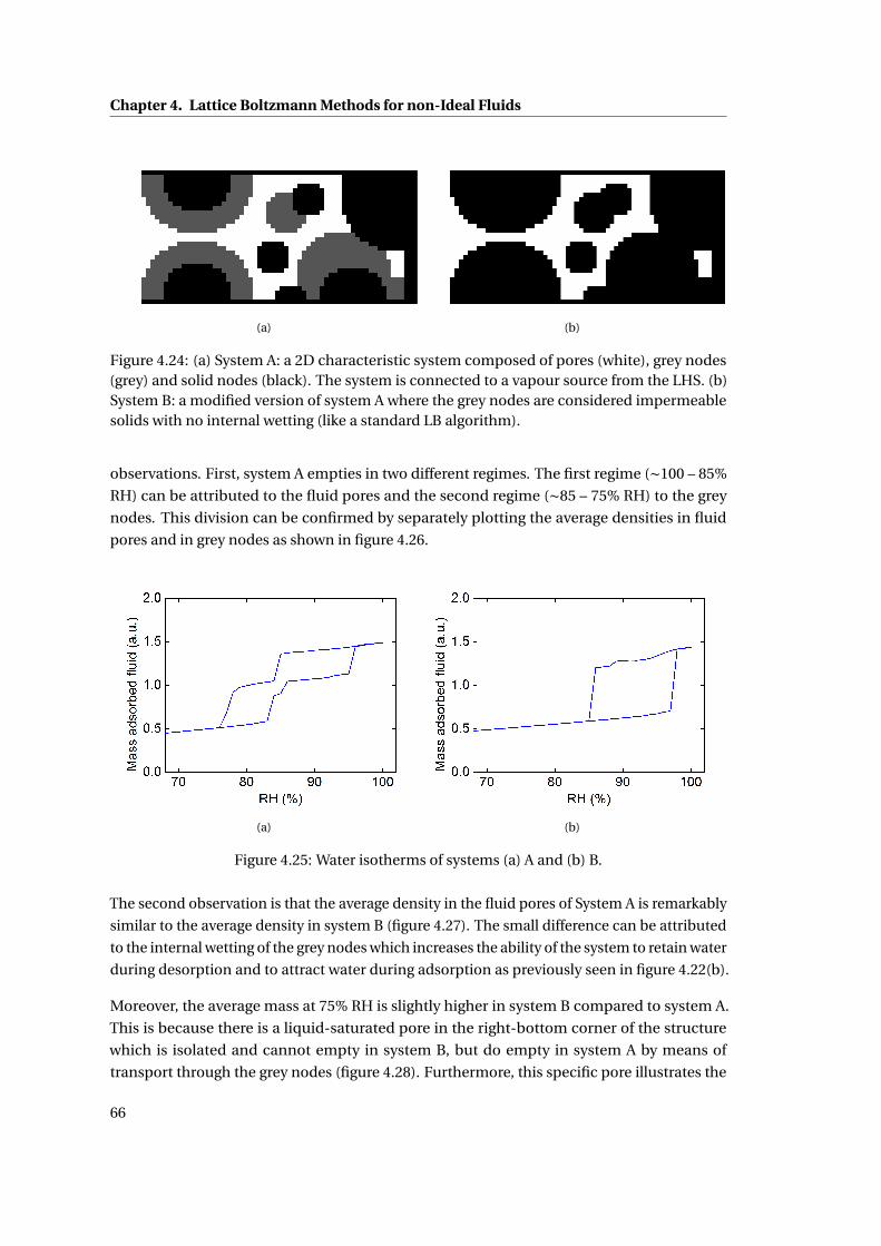
Chapter 4. Lattice Boltzmann Methods for non-Ideal Fluids
(a) (b)
Figure 4.24: (a) System A: a 2D characteristic system composed of pores (white), grey nodes(grey) and solid nodes (black). The system is connected to a vapour source from the LHS. (b)System B: a modified version of system A where the grey nodes are considered impermeablesolids with no internal wetting (like a standard LB algorithm).
observations. First, system A empties in two different regimes. The first regime (∼100 – 85%
RH) can be attributed to the fluid pores and the second regime (∼85 – 75% RH) to the grey
nodes. This division can be confirmed by separately plotting the average densities in fluid
pores and in grey nodes as shown in figure 4.26.
(a) (b)
Figure 4.25: Water isotherms of systems (a) A and (b) B.
The second observation is that the average density in the fluid pores of System A is remarkably
similar to the average density in system B (figure 4.27). The small difference can be attributed
to the internal wetting of the grey nodes which increases the ability of the system to retain water
during desorption and to attract water during adsorption as previously seen in figure 4.22(b).
Moreover, the average mass at 75% RH is slightly higher in system B compared to system A.
This is because there is a liquid-saturated pore in the right-bottom corner of the structure
which is isolated and cannot empty in system B, but do empty in system A by means of
transport through the grey nodes (figure 4.28). Furthermore, this specific pore illustrates the
66
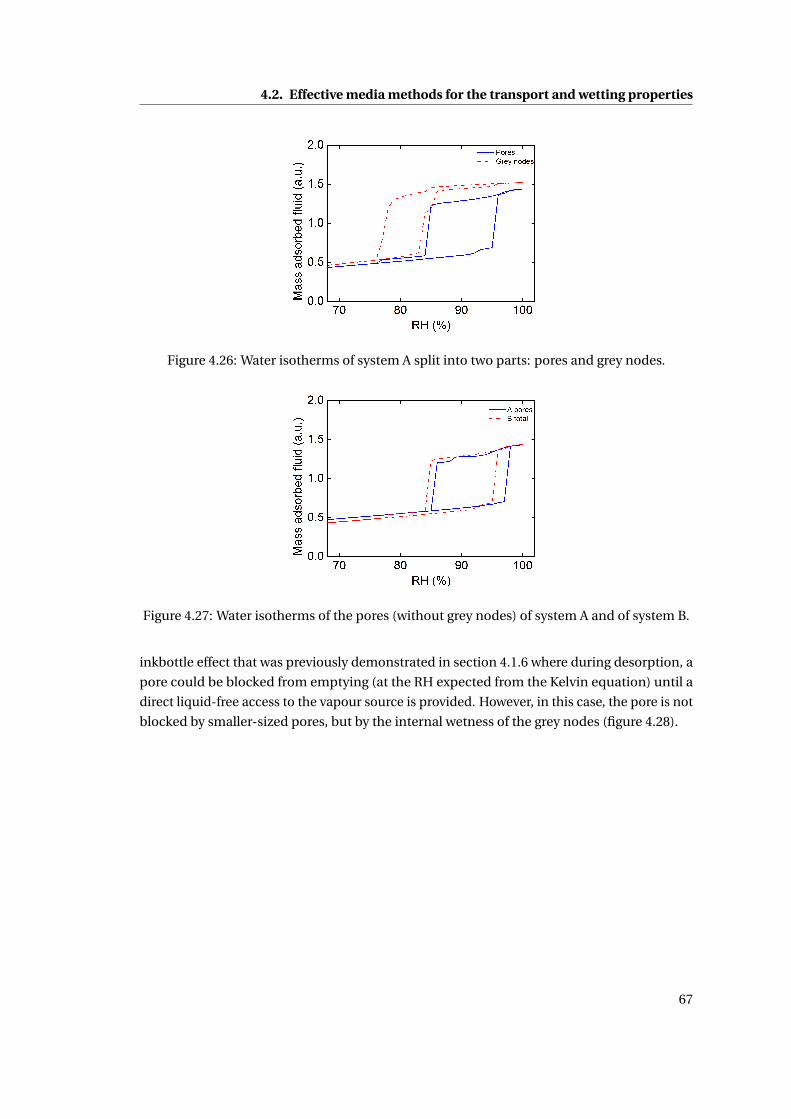
4.2. Effective media methods for the transport and wetting properties
Figure 4.26: Water isotherms of system A split into two parts: pores and grey nodes.
Figure 4.27: Water isotherms of the pores (without grey nodes) of system A and of system B.
inkbottle effect that was previously demonstrated in section 4.1.6 where during desorption, a
pore could be blocked from emptying (at the RH expected from the Kelvin equation) until a
direct liquid-free access to the vapour source is provided. However, in this case, the pore is not
blocked by smaller-sized pores, but by the internal wetness of the grey nodes (figure 4.28).
67
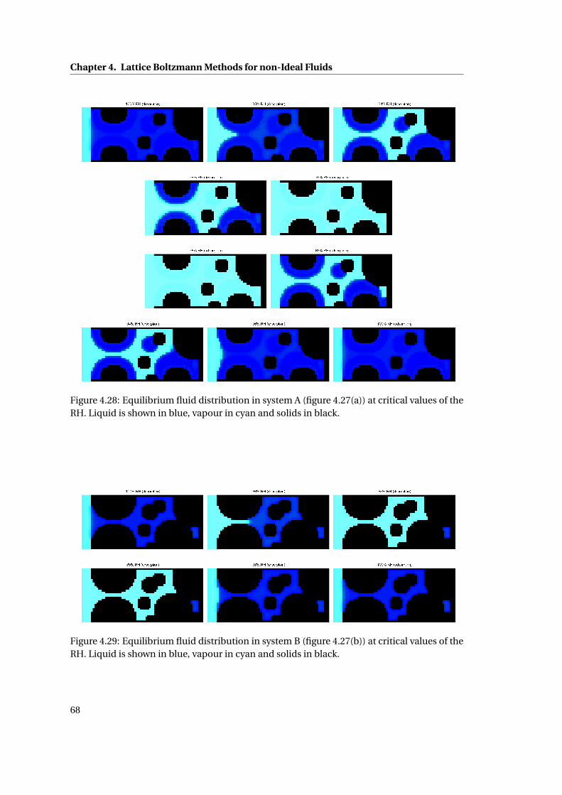
Chapter 4. Lattice Boltzmann Methods for non-Ideal Fluids
Figure 4.28: Equilibrium fluid distribution in system A (figure 4.27(a)) at critical values of theRH. Liquid is shown in blue, vapour in cyan and solids in black.
Figure 4.29: Equilibrium fluid distribution in system B (figure 4.27(b)) at critical values of theRH. Liquid is shown in blue, vapour in cyan and solids in black.
68
4.2. Effective media methods for the transport and wetting properties
4.2.7 Conclusions
In this section, a novel lattice Boltzmann model was proposed, implemented within a free en-
ergy framework, and validated. The model combines the advantages of the methods presented
in chapter 3 section 3.2 and in section 4.1.2 of this chapter. The model allows successful:
1. Description of the fluid with an equation of state and an implicit tracking of the liquid –
vapour interfaces.
2. Description of the fluid / solid boundaries with a wetting potential that defines the
contact angle.
3. Introduction of grey nodes with:
(a) Effective transport properties: the effective media parameter σg r e y is mathemati-
cally linked with the intrinsic permeability κg r e y of the grey nodes.
(b) Effective wetting properties: the internal wetting potential φg r e y is linked with
the water isotherms of the grey nodes. This wetting potential could ultimately be
mathematically linked with a characteristic pore size, just as the effective media
parameter was mathematically linked with the intrinsic permeability.
4. Description of the interactions that arise following the introduction of grey nodes: the
fluid / grey and the grey / solid boundaries are characterized with wetting potentials
that define the corresponding contact angles.
Finally, the ability of the method was demonstrated in section 4.2.6 where it was applied to
study the water isotherms of pseudo-random systems. The simulations captured a two-step
isotherm (figure 4.25(a)) and the ink-bottle effect during desorption (figure 4.28). This ability
will be further demonstrated in chapter 6 where the method will be used to model the water
isotherms of 3D model microstructures of cement paste.
69

5 Permeability of Cement Paste
Contents
5.1 Saturated permeability of cement paste . . . . . . . . . . . . . . . . . . . . . . 71
5.1.1 Cement paste model microstructures . . . . . . . . . . . . . . . . . . . . 71
5.1.2 Reproducibility of the permeability . . . . . . . . . . . . . . . . . . . . . 72
5.1.3 Permeability of cement paste model microstructures . . . . . . . . . . . 73
5.1.4 Lattice magnification and microstructural resolution . . . . . . . . . . . 75
5.1.5 Diagonal leaks . . . . . . . . . . . . . . . . . . . . . . . . . . . . . . . . . . 77
5.1.6 Comparison of µic and CEMHYD3D . . . . . . . . . . . . . . . . . . . . . 78
5.1.7 Comparison of µic and HYMOSTRUC3D . . . . . . . . . . . . . . . . . . 78
5.1.8 Conclusions . . . . . . . . . . . . . . . . . . . . . . . . . . . . . . . . . . . 79
5.2 Unsaturated permeability of cement paste . . . . . . . . . . . . . . . . . . . . 80
5.2.1 Cement paste model microstructures . . . . . . . . . . . . . . . . . . . . 80
5.2.2 Model microstructures at reduced degrees of water saturation . . . . . 81
5.2.3 Permeating fluid: accessible pore network and permeability of the C-S-H 82
5.2.4 Apparent permeability of cement paste model microstructures . . . . . 83
5.2.5 Discussion . . . . . . . . . . . . . . . . . . . . . . . . . . . . . . . . . . . . 85
5.2.6 Conclusions . . . . . . . . . . . . . . . . . . . . . . . . . . . . . . . . . . . 86
5.1 Saturated permeability of cement paste∗
5.1.1 Cement paste model microstructures
Cement paste model microstructures (100µm)3 in size were created using the vector model
µic [45, 106]. Structures were generated with water-to-cement (w/c) ratios ranging from 0.3
∗The following results were published by the author in: M. Zalzale and P.J. McDonald, Lattice Boltzmannsimulations of the permeability and capillary adsorption of cement model microstructures, Cement and ConcreteResearch, vol. 42, no. 12, pp. 1601–1610, 2012.
71
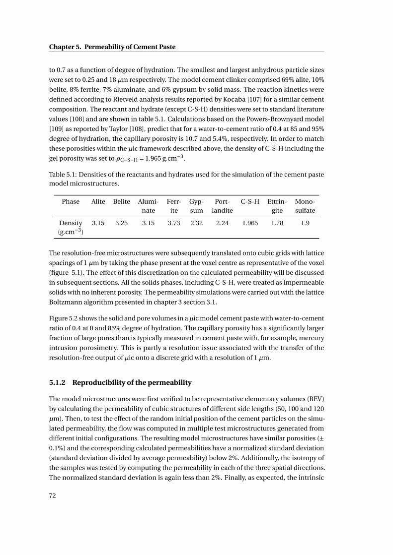
Chapter 5. Permeability of Cement Paste
to 0.7 as a function of degree of hydration. The smallest and largest anhydrous particle sizes
were set to 0.25 and 18 µm respectively. The model cement clinker comprised 69% alite, 10%
belite, 8% ferrite, 7% aluminate, and 6% gypsum by solid mass. The reaction kinetics were
defined according to Rietveld analysis results reported by Kocaba [107] for a similar cement
composition. The reactant and hydrate (except C-S-H) densities were set to standard literature
values [108] and are shown in table 5.1. Calculations based on the Powers-Brownyard model
[109] as reported by Taylor [108], predict that for a water-to-cement ratio of 0.4 at 85 and 95%
degree of hydration, the capillary porosity is 10.7 and 5.4%, respectively. In order to match
these porosities within the µic framework described above, the density of C-S-H including the
gel porosity was set to ρC−S−H = 1.965 g.cm−3.
Table 5.1: Densities of the reactants and hydrates used for the simulation of the cement pastemodel microstructures.
Phase Alite Belite Alumi- Ferr- Gyp- Port- C-S-H Ettrin- Mono-nate ite sum landite gite sulfate
Density 3.15 3.25 3.15 3.73 2.32 2.24 1.965 1.78 1.9(g.cm−3)
The resolution-free microstructures were subsequently translated onto cubic grids with lattice
spacings of 1 µm by taking the phase present at the voxel centre as representative of the voxel
(figure 5.1). The effect of this discretization on the calculated permeability will be discussed
in subsequent sections. All the solids phases, including C-S-H, were treated as impermeable
solids with no inherent porosity. The permeability simulations were carried out with the lattice
Boltzmann algorithm presented in chapter 3 section 3.1.
Figure 5.2 shows the solid and pore volumes in aµic model cement paste with water-to-cement
ratio of 0.4 at 0 and 85% degree of hydration. The capillary porosity has a significantly larger
fraction of large pores than is typically measured in cement paste with, for example, mercury
intrusion porosimetry. This is partly a resolution issue associated with the transfer of the
resolution-free output of µic onto a discrete grid with a resolution of 1 µm.
5.1.2 Reproducibility of the permeability
The model microstructures were first verified to be representative elementary volumes (REV)
by calculating the permeability of cubic structures of different side lengths (50, 100 and 120
µm). Then, to test the effect of the random initial position of the cement particles on the simu-
lated permeability, the flow was computed in multiple test microstructures generated from
different initial configurations. The resulting model microstructures have similar porosities (±0.1%) and the corresponding calculated permeabilities have a normalized standard deviation
(standard deviation divided by average permeability) below 2%. Additionally, the isotropy of
the samples was tested by computing the permeability in each of the three spatial directions.
The normalized standard deviation is again less than 2%. Finally, as expected, the intrinsic
72
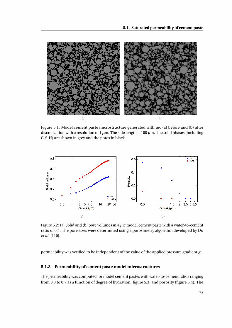
5.1. Saturated permeability of cement paste
(a) (b)
Figure 5.1: Model cement paste microstructure generated with µic (a) before and (b) afterdiscretization with a resolution of 1 µm. The side length is 100 µm. The solid phases (includingC-S-H) are shown in grey and the pores in black.
(a) (b)
Figure 5.2: (a) Solid and (b) pore volumes in a µic model cement paste with a water-to-cementratio of 0.4. The pore sizes were determined using a porosimetry algorithm developed by Doet al. [110].
permeability was verified to be independent of the value of the applied pressure gradient g .
5.1.3 Permeability of cement paste model microstructures
The permeability was computed for model cement pastes with water-to-cement ratios ranging
from 0.3 to 0.7 as a function of degree of hydration (figure 5.3) and porosity (figure 5.4). The
73
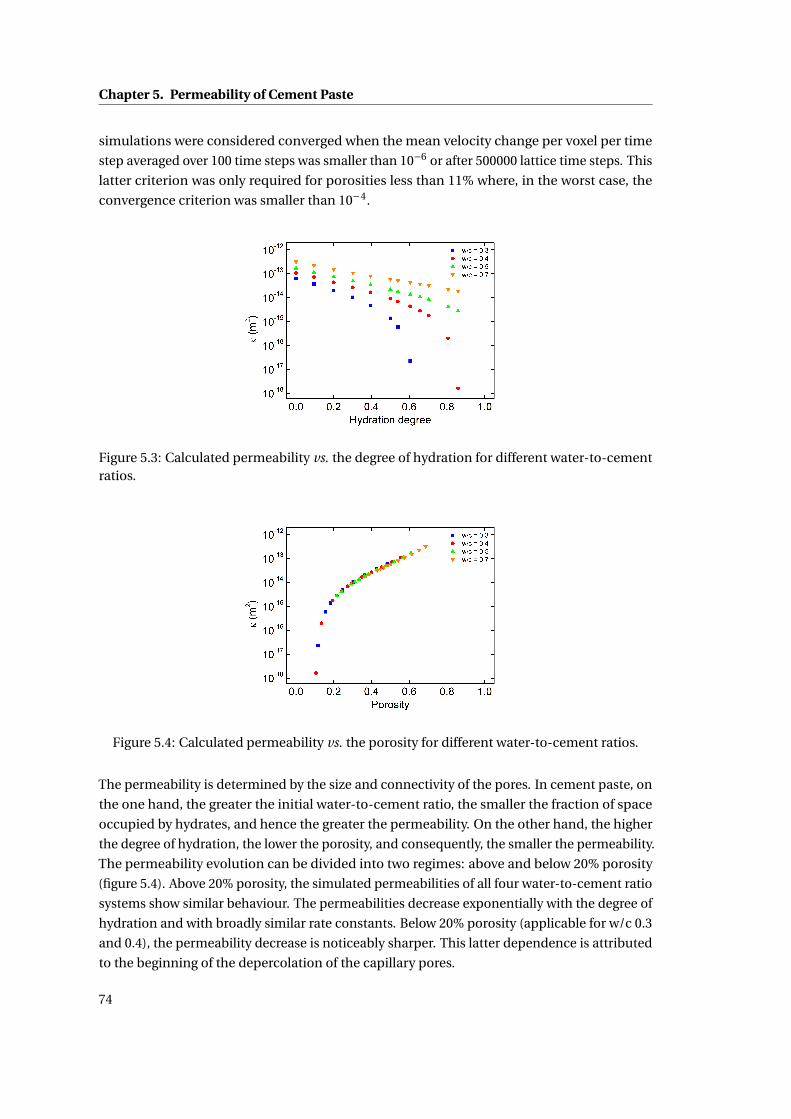
Chapter 5. Permeability of Cement Paste
simulations were considered converged when the mean velocity change per voxel per time
step averaged over 100 time steps was smaller than 10−6 or after 500000 lattice time steps. This
latter criterion was only required for porosities less than 11% where, in the worst case, the
convergence criterion was smaller than 10−4.
Figure 5.3: Calculated permeability vs. the degree of hydration for different water-to-cementratios.
Figure 5.4: Calculated permeability vs. the porosity for different water-to-cement ratios.
The permeability is determined by the size and connectivity of the pores. In cement paste, on
the one hand, the greater the initial water-to-cement ratio, the smaller the fraction of space
occupied by hydrates, and hence the greater the permeability. On the other hand, the higher
the degree of hydration, the lower the porosity, and consequently, the smaller the permeability.
The permeability evolution can be divided into two regimes: above and below 20% porosity
(figure 5.4). Above 20% porosity, the simulated permeabilities of all four water-to-cement ratio
systems show similar behaviour. The permeabilities decrease exponentially with the degree of
hydration and with broadly similar rate constants. Below 20% porosity (applicable for w/c 0.3
and 0.4), the permeability decrease is noticeably sharper. This latter dependence is attributed
to the beginning of the depercolation of the capillary pores.
74
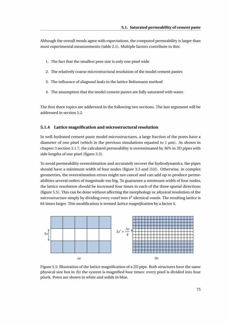
5.1. Saturated permeability of cement paste
Although the overall trends agree with expectations, the computed permeability is larger than
most experimental measurements (table 2.1). Multiple factors contribute to this:
1. The fact that the smallest pore size is only one pixel wide
2. The relatively coarse microstructural resolution of the model cement pastes
3. The influence of diagonal leaks in the lattice Boltzmann method
4. The assumption that the model cement pastes are fully saturated with water.
The first three topics are addressed in the following two sections. The last argument will be
addressed in section 5.2.
5.1.4 Lattice magnification and microstructural resolution
In well-hydrated cement paste model microstructures, a large fraction of the pores have a
diameter of one pixel (which in the previous simulations equated to 1 µm). As shown in
chapter 3 section 3.1.7, the calculated permeability is overestimated by 36% in 3D pipes with
side lengths of one pixel (figure 3.3).
To avoid permeability overestimation and accurately recover the hydrodynamics, the pipes
should have a minimum width of four nodes (figure 3.3 and [53]). Otherwise, in complex
geometries, the overestimation errors might not cancel and can add up to produce perme-
abilities several orders of magnitude too big. To guarantee a minimum width of four nodes,
the lattice resolution should be increased four times in each of the three spatial directions
(figure 5.5). This can be done without affecting the morphology or physical resolution of the
microstructure simply by dividing every voxel into 43 identical voxels. The resulting lattice is
64 times larger. This modification is termed lattice magnification by a factor 4.
(a) (b)
Figure 5.5: Illustration of the lattice magnification of a 2D pipe. Both structures have the samephysical size but in (b) the system is magnified four times: every pixel is divided into fourpixels. Pores are shown in white and solids in blue.
75
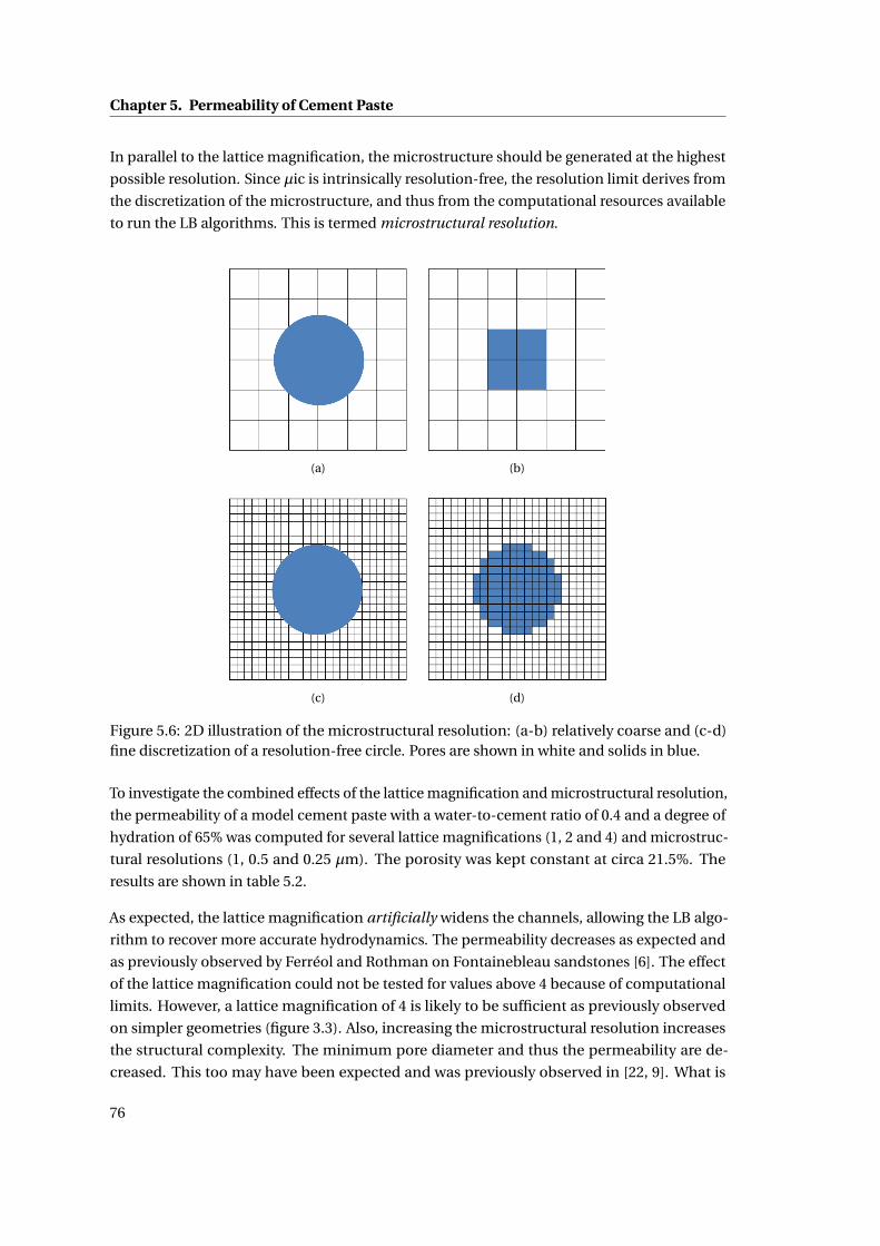
Chapter 5. Permeability of Cement Paste
In parallel to the lattice magnification, the microstructure should be generated at the highest
possible resolution. Since µic is intrinsically resolution-free, the resolution limit derives from
the discretization of the microstructure, and thus from the computational resources available
to run the LB algorithms. This is termed microstructural resolution.
(a) (b)
(c) (d)
Figure 5.6: 2D illustration of the microstructural resolution: (a-b) relatively coarse and (c-d)fine discretization of a resolution-free circle. Pores are shown in white and solids in blue.
To investigate the combined effects of the lattice magnification and microstructural resolution,
the permeability of a model cement paste with a water-to-cement ratio of 0.4 and a degree of
hydration of 65% was computed for several lattice magnifications (1, 2 and 4) and microstruc-
tural resolutions (1, 0.5 and 0.25 µm). The porosity was kept constant at circa 21.5%. The
results are shown in table 5.2.
As expected, the lattice magnification artificially widens the channels, allowing the LB algo-
rithm to recover more accurate hydrodynamics. The permeability decreases as expected and
as previously observed by Ferréol and Rothman on Fontainebleau sandstones [6]. The effect
of the lattice magnification could not be tested for values above 4 because of computational
limits. However, a lattice magnification of 4 is likely to be sufficient as previously observed
on simpler geometries (figure 3.3). Also, increasing the microstructural resolution increases
the structural complexity. The minimum pore diameter and thus the permeability are de-
creased. This too may have been expected and was previously observed in [22, 9]. What is
76
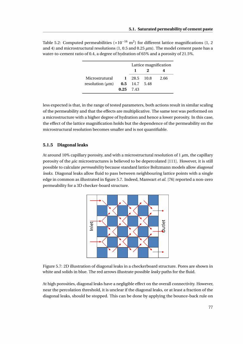
5.1. Saturated permeability of cement paste
Table 5.2: Computed permeabilities (×10−16 m2) for different lattice magnifications (1, 2and 4) and microstructural resolutions (1, 0.5 and 0.25 µm). The model cement paste has awater-to-cement ratio of 0.4, a degree of hydration of 65% and a porosity of 21.5%.
Lattice magnification1 2 4
Microstrutural 1 28.5 10.8 2.66resolution (µm) 0.5 14.7 5.48
0.25 7.43
less expected is that, in the range of tested parameters, both actions result in similar scaling
of the permeability and that the effects are multiplicative. The same test was performed on
a microstructure with a higher degree of hydration and hence a lower porosity. In this case,
the effect of the lattice magnification holds but the dependence of the permeability on the
microstructural resolution becomes smaller and is not quantifiable.
5.1.5 Diagonal leaks
At around 10% capillary porosity, and with a microstructural resolution of 1 µm, the capillary
porosity of the µic microstructures is believed to be depercolated [111]. However, it is still
possible to calculate permeability because standard lattice Boltzmann models allow diagonal
leaks. Diagonal leaks allow fluid to pass between neighbouring lattice points with a single
edge in common as illustrated in figure 5.7. Indeed, Manwart et al. [76] reported a non-zero
permeability for a 3D checker-board structure.
Figure 5.7: 2D illustration of diagonal leaks in a checkerboard structure. Pores are shown inwhite and solids in blue. The red arrows illustrate possible leaky paths for the fluid.
At high porosities, diagonal leaks have a negligible effect on the overall connectivity. However,
near the percolation threshold, it is unclear if the diagonal leaks, or at least a fraction of the
diagonal leaks, should be stopped. This can be done by applying the bounce-back rule on
77
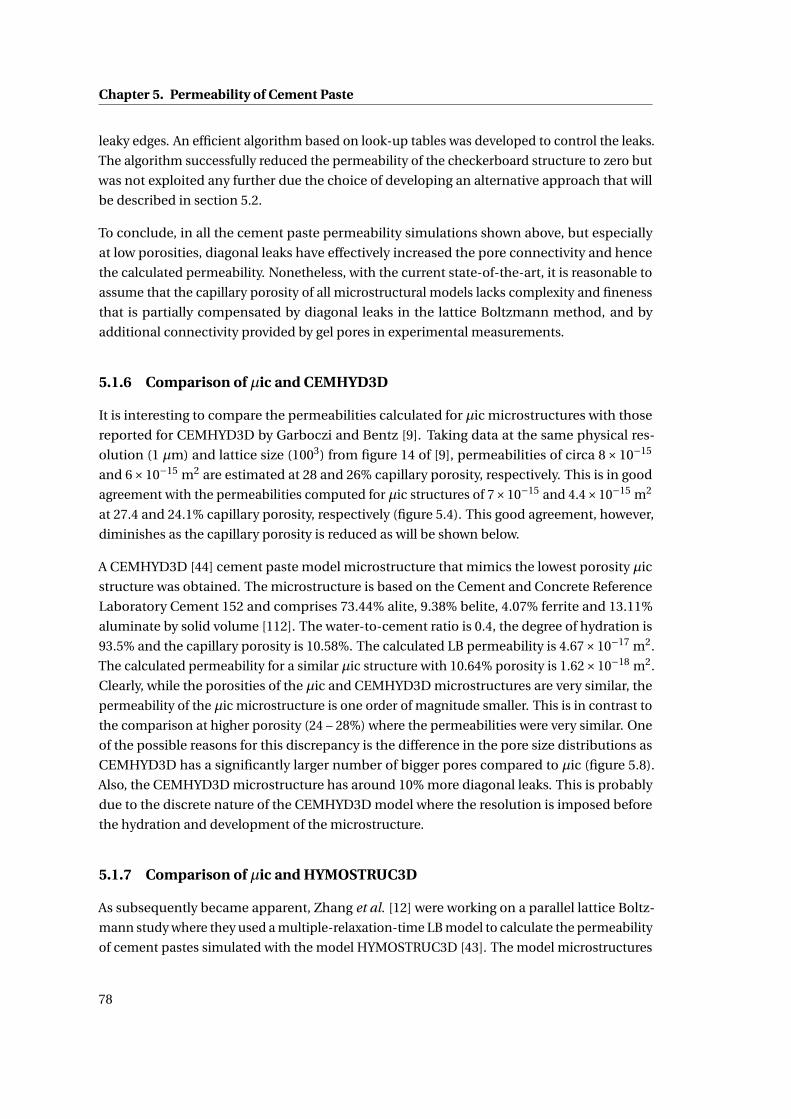
Chapter 5. Permeability of Cement Paste
leaky edges. An efficient algorithm based on look-up tables was developed to control the leaks.
The algorithm successfully reduced the permeability of the checkerboard structure to zero but
was not exploited any further due the choice of developing an alternative approach that will
be described in section 5.2.
To conclude, in all the cement paste permeability simulations shown above, but especially
at low porosities, diagonal leaks have effectively increased the pore connectivity and hence
the calculated permeability. Nonetheless, with the current state-of-the-art, it is reasonable to
assume that the capillary porosity of all microstructural models lacks complexity and fineness
that is partially compensated by diagonal leaks in the lattice Boltzmann method, and by
additional connectivity provided by gel pores in experimental measurements.
5.1.6 Comparison of µic and CEMHYD3D
It is interesting to compare the permeabilities calculated for µic microstructures with those
reported for CEMHYD3D by Garboczi and Bentz [9]. Taking data at the same physical res-
olution (1 µm) and lattice size (1003) from figure 14 of [9], permeabilities of circa 8×10⁻¹⁵
and 6×10⁻¹⁵ m2 are estimated at 28 and 26% capillary porosity, respectively. This is in good
agreement with the permeabilities computed for µic structures of 7×10⁻¹⁵ and 4.4×10⁻¹⁵ m2
at 27.4 and 24.1% capillary porosity, respectively (figure 5.4). This good agreement, however,
diminishes as the capillary porosity is reduced as will be shown below.
A CEMHYD3D [44] cement paste model microstructure that mimics the lowest porosity µic
structure was obtained. The microstructure is based on the Cement and Concrete Reference
Laboratory Cement 152 and comprises 73.44% alite, 9.38% belite, 4.07% ferrite and 13.11%
aluminate by solid volume [112]. The water-to-cement ratio is 0.4, the degree of hydration is
93.5% and the capillary porosity is 10.58%. The calculated LB permeability is 4.67×10⁻¹⁷ m2.
The calculated permeability for a similar µic structure with 10.64% porosity is 1.62×10⁻¹⁸ m2.
Clearly, while the porosities of the µic and CEMHYD3D microstructures are very similar, the
permeability of the µic microstructure is one order of magnitude smaller. This is in contrast to
the comparison at higher porosity (24 – 28%) where the permeabilities were very similar. One
of the possible reasons for this discrepancy is the difference in the pore size distributions as
CEMHYD3D has a significantly larger number of bigger pores compared to µic (figure 5.8).
Also, the CEMHYD3D microstructure has around 10% more diagonal leaks. This is probably
due to the discrete nature of the CEMHYD3D model where the resolution is imposed before
the hydration and development of the microstructure.
5.1.7 Comparison of µic and HYMOSTRUC3D
As subsequently became apparent, Zhang et al. [12] were working on a parallel lattice Boltz-
mann study where they used a multiple-relaxation-time LB model to calculate the permeability
of cement pastes simulated with the model HYMOSTRUC3D [43]. The model microstructures
78
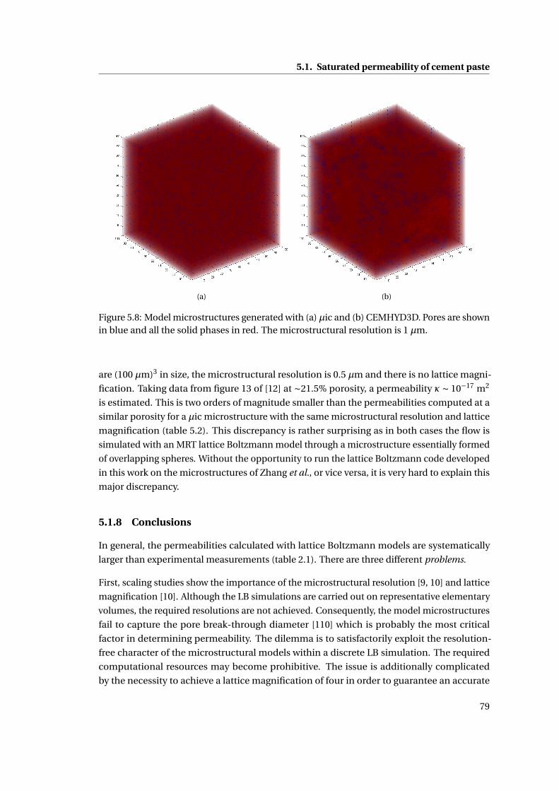
5.1. Saturated permeability of cement paste
(a) (b)
Figure 5.8: Model microstructures generated with (a) µic and (b) CEMHYD3D. Pores are shownin blue and all the solid phases in red. The microstructural resolution is 1 µm.
are (100 µm)3 in size, the microstructural resolution is 0.5 µm and there is no lattice magni-
fication. Taking data from figure 13 of [12] at ∼21.5% porosity, a permeability κ∼ 10−17 m2
is estimated. This is two orders of magnitude smaller than the permeabilities computed at a
similar porosity for a µic microstructure with the same microstructural resolution and lattice
magnification (table 5.2). This discrepancy is rather surprising as in both cases the flow is
simulated with an MRT lattice Boltzmann model through a microstructure essentially formed
of overlapping spheres. Without the opportunity to run the lattice Boltzmann code developed
in this work on the microstructures of Zhang et al., or vice versa, it is very hard to explain this
major discrepancy.
5.1.8 Conclusions
In general, the permeabilities calculated with lattice Boltzmann models are systematically
larger than experimental measurements (table 2.1). There are three different problems.
First, scaling studies show the importance of the microstructural resolution [9, 10] and lattice
magnification [10]. Although the LB simulations are carried out on representative elementary
volumes, the required resolutions are not achieved. Consequently, the model microstructures
fail to capture the pore break-through diameter [110] which is probably the most critical
factor in determining permeability. The dilemma is to satisfactorily exploit the resolution-
free character of the microstructural models within a discrete LB simulation. The required
computational resources may become prohibitive. The issue is additionally complicated
by the necessity to achieve a lattice magnification of four in order to guarantee an accurate
79
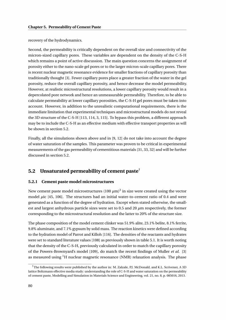
Chapter 5. Permeability of Cement Paste
recovery of the hydrodynamics.
Second, the permeability is critically dependent on the overall size and connectivity of the
micron-sized capillary pores. These variables are dependent on the density of the C-S-H
which remains a point of active discussion. The main question concerns the assignment of
porosity either to the nano-scale gel pores or to the larger micron-scale capillary pores. There
is recent nuclear magnetic resonance evidence for smaller fractions of capillary porosity than
traditionally thought [3]. Fewer capillary pores place a greater fraction of the water in the gel
porosity, reduce the overall capillary porosity, and hence decrease the model permeability.
However, at realistic microstructural resolutions, a lower capillary porosity would result in a
depercolated pore network and hence an unmeasurable permeability. Therefore, to be able to
calculate permeability at lower capillary porosities, the C-S-H gel pores must be taken into
account. However, in addition to the unrealistic computational requirements, there is the
immediate limitation that experimental techniques and microstructural models do not reveal
the 3D structure of the C-S-H [113, 114, 3, 115]. To bypass this problem, a different approach
may be to include the C-S-H as an effective medium with effective transport properties as will
be shown in section 5.2.
Finally, all the simulations shown above and in [9, 12] do not take into account the degree
of water saturation of the samples. This parameter was proven to be critical in experimental
measurements of the gas permeability of cementitious materials [31, 33, 32] and will be further
discussed in section 5.2.
5.2 Unsaturated permeability of cement paste†
5.2.1 Cement paste model microstructures
New cement paste model microstructures (100 µm)3 in size were created using the vector
model µic [45, 106]. The structures had an initial water-to-cement ratio of 0.4 and were
generated as a function of the degree of hydration. Except when stated otherwise, the small-
est and largest anhydrous particle sizes were set to 0.5 and 20 µm respectively, the former
corresponding to the microstructural resolution and the latter to 20% of the structure size.
The phase composition of the model cement clinker was 51.9% alite, 23.1% belite, 8.1% ferrite,
9.8% aluminate, and 7.1% gypsum by solid mass. The reaction kinetics were defined according
to the hydration model of Parrot and Killoh [116]. The densities of the reactants and hydrates
were set to standard literature values [108] as previously shown in table 5.1. It is worth noting
that the density of the C-S-H, previously calculated in order to match the capillary porosity
of the Powers-Brownyard’s model [109], do match the recent findings of Muller et al. [3]
as measured using 1H nuclear magnetic resonance (NMR) relaxation analysis. The phase
†The following results were published by the author in: M. Zalzale, P.J. McDonald, and K.L. Scrivener, A 3Dlattice Boltzmann effective media study: understanding the role of C-S-H and water saturation on the permeabilityof cement paste, Modelling and Simulation in Materials Science and Engineering, vol. 21, no. 8, p. 085016, 2013.
80
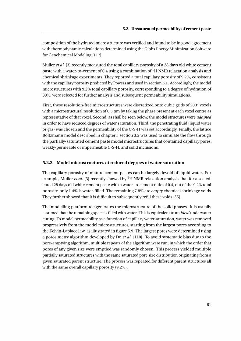
5.2. Unsaturated permeability of cement paste
composition of the hydrated microstructure was verified and found to be in good agreement
with thermodynamic calculations determined using the Gibbs Energy Minimization Software
for Geochemical Modeling [117].
Muller et al. [3] recently measured the total capillary porosity of a 28 days old white cement
paste with a water-to-cement of 0.4 using a combination of 1H NMR relaxation analysis and
chemical shrinkage experiments. They reported a total capillary porosity of 9.2%, consistent
with the capillary porosity predicted by Powers and used in section 5.1. Accordingly, the model
microstructures with 9.2% total capillary porosity, corresponding to a degree of hydration of
89%, were selected for further analysis and subsequent permeability simulations.
First, these resolution-free microstructures were discretized onto cubic grids of 2003 voxels
with a microstructural resolution of 0.5 µm by taking the phase present at each voxel centre as
representative of that voxel. Second, as shall be seen below, the model structures were adapted
in order to have reduced degrees of water saturation. Third, the penetrating fluid (liquid water
or gas) was chosen and the permeability of the C-S-H was set accordingly. Finally, the lattice
Boltzmann model described in chapter 3 section 3.2 was used to simulate the flow through
the partially-saturated cement paste model microstructures that contained capillary pores,
weakly-permeable or impermeable C-S-H, and solid inclusions.
5.2.2 Model microstructures at reduced degrees of water saturation
The capillary porosity of mature cement pastes can be largely devoid of liquid water. For
example, Muller et al. [3] recently showed by 1H NMR relaxation analysis that for a sealed-
cured 28 days old white cement paste with a water-to-cement ratio of 0.4, out of the 9.2% total
porosity, only 1.4% is water-filled. The remaining 7.8% are empty chemical shrinkage voids.
They further showed that it is difficult to subsequently refill these voids [35].
The modelling platform µic generates the microstructure of the solid phases. It is usually
assumed that the remaining space is filled with water. This is equivalent to an ideal underwater
curing. To model permeability as a function of capillary water saturation, water was removed
progressively from the model microstructures, starting from the largest pores according to
the Kelvin-Laplace law, as illustrated in figure 5.9. The largest pores were determined using
a porosimetry algorithm developed by Do et al. [110]. To avoid systematic bias due to the
pore-emptying algorithm, multiple repeats of the algorithm were run, in which the order that
pores of any given size were emptied was randomly chosen. This process yielded multiple
partially saturated structures with the same saturated pore size distribution originating from a
given saturated parent structure. The process was repeated for different parent structures all
with the same overall capillary porosity (9.2%).
81
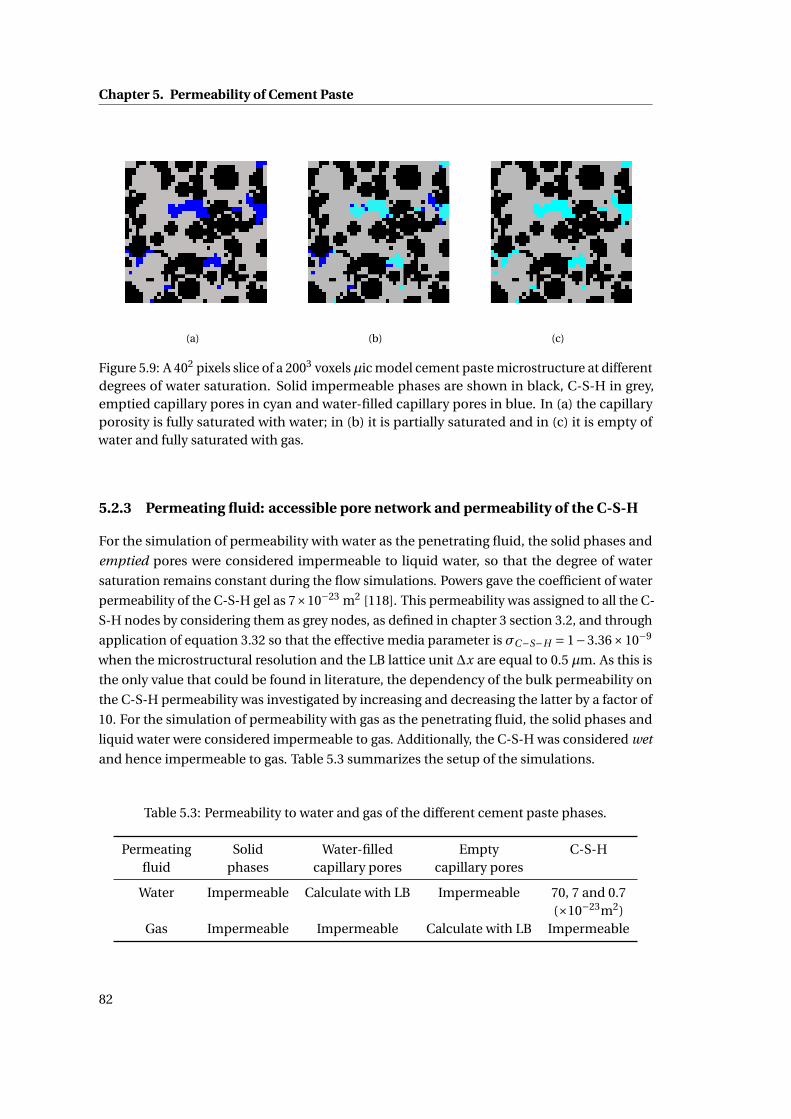
Chapter 5. Permeability of Cement Paste
(a) (b) (c)
Figure 5.9: A 402 pixels slice of a 2003 voxelsµic model cement paste microstructure at differentdegrees of water saturation. Solid impermeable phases are shown in black, C-S-H in grey,emptied capillary pores in cyan and water-filled capillary pores in blue. In (a) the capillaryporosity is fully saturated with water; in (b) it is partially saturated and in (c) it is empty ofwater and fully saturated with gas.
5.2.3 Permeating fluid: accessible pore network and permeability of the C-S-H
For the simulation of permeability with water as the penetrating fluid, the solid phases and
emptied pores were considered impermeable to liquid water, so that the degree of water
saturation remains constant during the flow simulations. Powers gave the coefficient of water
permeability of the C-S-H gel as 7×10⁻²³ m2 [118]. This permeability was assigned to all the C-
S-H nodes by considering them as grey nodes, as defined in chapter 3 section 3.2, and through
application of equation 3.32 so that the effective media parameter is σC−S−H = 1−3.36×10⁻⁹
when the microstructural resolution and the LB lattice unit ∆x are equal to 0.5 µm. As this is
the only value that could be found in literature, the dependency of the bulk permeability on
the C-S-H permeability was investigated by increasing and decreasing the latter by a factor of
10. For the simulation of permeability with gas as the penetrating fluid, the solid phases and
liquid water were considered impermeable to gas. Additionally, the C-S-H was considered wet
and hence impermeable to gas. Table 5.3 summarizes the setup of the simulations.
Table 5.3: Permeability to water and gas of the different cement paste phases.
Permeating Solid Water-filled Empty C-S-Hfluid phases capillary pores capillary pores
Water Impermeable Calculate with LB Impermeable 70, 7 and 0.7(×10−23m2)
Gas Impermeable Impermeable Calculate with LB Impermeable
82
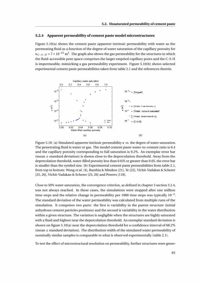
5.2. Unsaturated permeability of cement paste
5.2.4 Apparent permeability of cement paste model microstructures
Figure 5.10(a) shows the cement paste apparent intrinsic permeability with water as the
permeating fluid as a function of the degree of water saturation of the capillary porosity for
κC−S−H = 7×10⁻²³ m2. The graph also shows the gas permeability for the structures in which
the fluid-accessible pore space comprises the larger emptied capillary pores and the C-S-H
is impermeable, mimicking a gas permeability experiment. Figure 5.10(b) shows selected
experimental cement paste permeabilities taken from table 2.1 and the references therein.
(a) (b)
Figure 5.10: (a) Simulated apparent intrinsic permeability κ vs. the degree of water saturation.The penetrating fluid is water or gas. The model cement paste water-to-cement ratio is 0.4and the capillary porosity corresponding to full saturation is 9.2%. An exemplar error bar(mean ± standard deviation) is shown close to the depercolation threshold. Away from thedepercolation threshold, water-filled porosity less than 0.035 or greater than 0.05, the error baris smaller than the symbol size. (b) Experimental cement paste permeabilities from table 2.1,from top to bottom: Wong et al. [4], Banthia & Mindess [21], Ye [22], Vichit-Vadakan & Scherer[25, 26], Vichit-Vadakan & Scherer [25, 26] and Powers [118].
Close to 50% water saturation, the convergence criterion, as defined in chapter 3 section 3.2.4,
was not always reached. In these cases, the simulations were stopped after one million
time steps and the relative change in permeability per 1000 time steps was typically 10−4.
The standard deviation of the water permeability was calculated from multiple runs of the
simulation. It comprises two parts: the first is variability in the parent structure (initial
anhydrous cement particles positions) and the second is variability in the water distribution
within a given structure. The variation is negligible when the structures are highly saturated
with a fluid and highest near the depercolation threshold. An exemplar standard deviation is
shown on figure 5.10(a) near the depercolation threshold for a confidence interval of 68.2%
(mean ± standard deviation). The distribution width of the simulated water permeability of
nominally similar samples is comparable to what is observed experimentally (table 2.1).
To test the effect of microstructural resolution on permeability, further structures were gener-
83
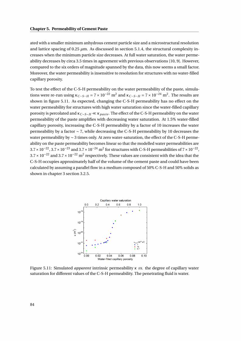
Chapter 5. Permeability of Cement Paste
ated with a smaller minimum anhydrous cement particle size and a microstructural resolution
and lattice spacing of 0.25 µm. As discussed in section 5.1.4, the structural complexity in-
creases when the minimum particle size decreases. At full water saturation, the water perme-
ability decreases by circa 3.5 times in agreement with previous observations [10, 9]. However,
compared to the six orders of magnitude spanned by the data, this now seems a small factor.
Moreover, the water permeability is insensitive to resolution for structures with no water-filled
capillary porosity.
To test the effect of the C-S-H permeability on the water permeability of the paste, simula-
tions were re-run using κC−S−H = 7×10⁻²² m2 and κC−S−H = 7×10⁻²⁴ m2. The results are
shown in figure 5.11. As expected, changing the C-S-H permeability has no effect on the
water permeability for structures with high water saturation since the water-filled capillary
porosity is percolated and κC−S−H ¿ κpaste . The effect of the C-S-H permeability on the water
permeability of the paste amplifies with decreasing water saturation. At 1.5% water-filled
capillary porosity, increasing the C-S-H permeability by a factor of 10 increases the water
permeability by a factor ∼ 7, while decreasing the C-S-H permeability by 10 decreases the
water permeability by ∼ 3 times only. At zero water-saturation, the effect of the C-S-H perme-
ability on the paste permeability becomes linear so that the modelled water permeabilities are
3.7×10⁻²², 3.7×10⁻²³ and 3.7×10⁻²⁴ m2 for structures with C-S-H permeabilities of 7×10⁻²²,
3.7×10⁻²² and 3.7×10⁻²² m2 respectively. These values are consistent with the idea that the
C-S-H occupies approximately half of the volume of the cement paste and could have been
calculated by assuming a parallel flow in a medium composed of 50% C-S-H and 50% solids as
shown in chapter 3 section 3.2.5.
Figure 5.11: Simulated apparent intrinsic permeability κ vs. the degree of capillary watersaturation for different values of the C-S-H permeability. The penetrating fluid is water.
84
5.2. Unsaturated permeability of cement paste
5.2.5 Discussion
The intrinsic permeability of the structure fully saturated with water is conceptually‡ the same
as the intrinsic permeability of a completely dried cement paste saturated with gas in an
ideal gas permeability experiment. It is therefore not surprising that, at high degrees of water
saturation, the water permeability is comparable to the oxygen permeability results of Wong et
al. [4]. Practically, a better comparison is with the simulation of the sister structure saturated
with gas (zero water saturation) since, in most laboratory gas experiments, the C-S-H is not
fully dried and is therefore impermeable to gas. In both cases, when the capillary porosity is
highly saturated with a fluid, the role of water within the C-S-H in determining permeability is
minimal as the flow is mainly controlled by the percolated fluid-filled capillary pores.
By gradually reducing the water saturation, the water permeability decreases. Initially the
decrease is slow. Below 60% capillary water saturation, the water permeability decreases
more rapidly as the water-filled capillary porosity starts to depercolate. A very sharp drop
in water permeability is observed between 50 and 40% water saturation regardless of the
C-S-H permeability. This is in agreement with the findings of Elam et al. [119] who reported
depercolation of the void regions between mono-sized overlapping spheres at around 3.2%
void. When the water-filled capillary porosity is depercolated, the influence of flow through
the weakly-permeable C-S-H is amplified because the flow is then mainly controlled by the
weakly-permeable C-S-H. The water permeability ranges from approximately 10−19 to 10−22
m2. This agrees well with the range of experimental water permeability measurements as
shown in table 2.1. It is therefore interesting to consider the likely degree of water saturation
of the samples in those experiments.
In the case of Ye [22], paste samples were sealed cured for 28 days and then vacuum saturated
with water for 4 to 8 hours before the water permeability measurement. Muller [35] reports
that for a 28 day sealed cured sample that was subsequently vacuum saturated for 24 hours,
the water-filled capillary porosity rose from 1.4 to 5.5% as measured by NMR. Since Ye’s
samples were vacuum saturated for a shorter time, a slightly smaller water-filled fraction
should be expected. In agreement with this expectation, the water permeability measurement
of Ye, 9.0×10⁻²¹ m2, is matched by a water permeability simulation with approximately 4.3%
water-filled capillary porosity for Powers measured value κC−S−H = 7×10⁻²³ m2.
Vichit-Vadakan and Scherer [25] used the beam-bending method to measure water permeabil-
ity in a range of samples of different sizes that were cured sealed for 48 hours and then further
cured underwater. Permeability is derived from the rate of relief of pressure required to bend a
water saturated sample. To verify that the samples were fully saturated, they compared the
permeability before and after pressurization underwater at 2 MPa for 24 hours. The authors
concluded that small samples were fully saturated prior to pressurization on the basis of con-
stancy of the permeability but that this was not the case for larger samples. However, a careful
examination of their figure 4 reveals that permeability decreased after pressurization by about
‡The intrinsic permeability is independent of the permeating fluid.
85
Chapter 5. Permeability of Cement Paste
20% for the smallest samples (5.7 mm) and by about 60% for slightly larger samples (7.7 mm).
As they suggest, one possible interpretation for higher permeability values before pressure
saturation is the relief of internal pressure by water flow into nearby air voids. We suggest that
even the small samples may not have been fully saturated before pressurization. Moreover,
those few samples that were subjected to pressurization may not have been fully saturated
either. Using the experimentally measured permeability and a pressure of 2 MPa, Darcy’s law
suggests that several days are required to fill the void spaces created during the preliminary
48 hours of sealed curing, rather than the single day allowed, even for the small samples.
In the LB simulations, the water permeability matches the experimental measurements of
Vichit-Vadakan and Scherer 5×10⁻²² to 10−21 m2 between 4 and 4.2% water-filled capillary
porosity again for κC−S−H = 7×10⁻²³ m2.
Overall, the effect of the C-S-H on the simulated permeability is partially seen in the detail
of the asymmetry of the liquid and gas curves in figure 5.10(a). This is because the C-S-H is
considered permeable in the former case, and impermeable in the latter. However, it is not
the full story, since the asymmetry is also due to the fact that at water saturation Sw , the liquid
occupies a different pore network (predominantly small pores) compared to the gas (large
pores) at saturation (1 – Sw ). The role of the C-S-H amplifies as the capillary porosity starts
to depercolate. This is unequivocally seen by comparing the current results with previous
LB water permeability simulations that treated the C-S-H as impermeable solid as seen in
section 5.1 and in [10, 9, 12]. In those calculations, as the porosity decreased by increasing
the degree of hydration, the permeability decreased monotonically and catastrophically
close the percolation threshold, below which it could not be calculated accurately and was
mainly a result of diagonal leaks. Now, however, the asymptotic approach towards a plateau
permeability dictated by the C-S-H is clearly seen.
5.2.6 Conclusions
This chapter addressed the shortcomings of the standard lattice Boltzmann methods as dis-
cussed in the conclusions of section 5.1. This chapter also allowed insights to be gained on the
possible reasons behind the large scatter in experimental measurements of the permeability
of cement paste.
First, the effective media lattice Boltzmann approach proved to be well suited to numerical
calculation of permeability within complex multi-scale 3D cement paste microstructures
including capillary pore regions of defined geometry, calcium silicate hydrate regions of
defined permeability, and impermeable solid inclusions. This is an advance over previous
numerical simulations of permeability in cement paste where only the capillary pore network
was considered, and further this was fully saturated.
The simulation of apparent intrinsic permeability at different degrees of water saturation
provides a very plausible explanation for the enormous range of experimental results. The
results also explain the apparently large values of water permeability reported in previous
86
5.2. Unsaturated permeability of cement paste
simulations without invoking earlier arguments of limited spatial resolution either in the
microstructure or in the lattice Boltzmann solver. It is now clear that the large permeability is
a direct consequence of the percolation of the capillary pore network at full water saturation.
The suggestion is that most experimental measurements with water are not conducted on
fully saturated samples. The presence of air voids in nominally water saturated samples could
lower dramatically their apparent intrinsic permeability. It is further concluded that the role
of the weakly-permeable C-S-H, omitted in earlier modelling studies, is critical and has a
non-linear effect on the permeability of cement paste.
Finally, while both liquid water and gas permeabilities were calculated, a multi-phase fluid
with an equation of state that links liquid water and vapour is yet to be incorporated in the
lattice Boltzmann model. This modification would remove the necessity for the assumption
that the degree of water saturation remains constant during the flow simulations. A multi-
phase model was introduced in chapter 4 and is the subject of the following chapter where
the objective is to study the adsorption and desorption of water and vapour in model cement
pastes.
87

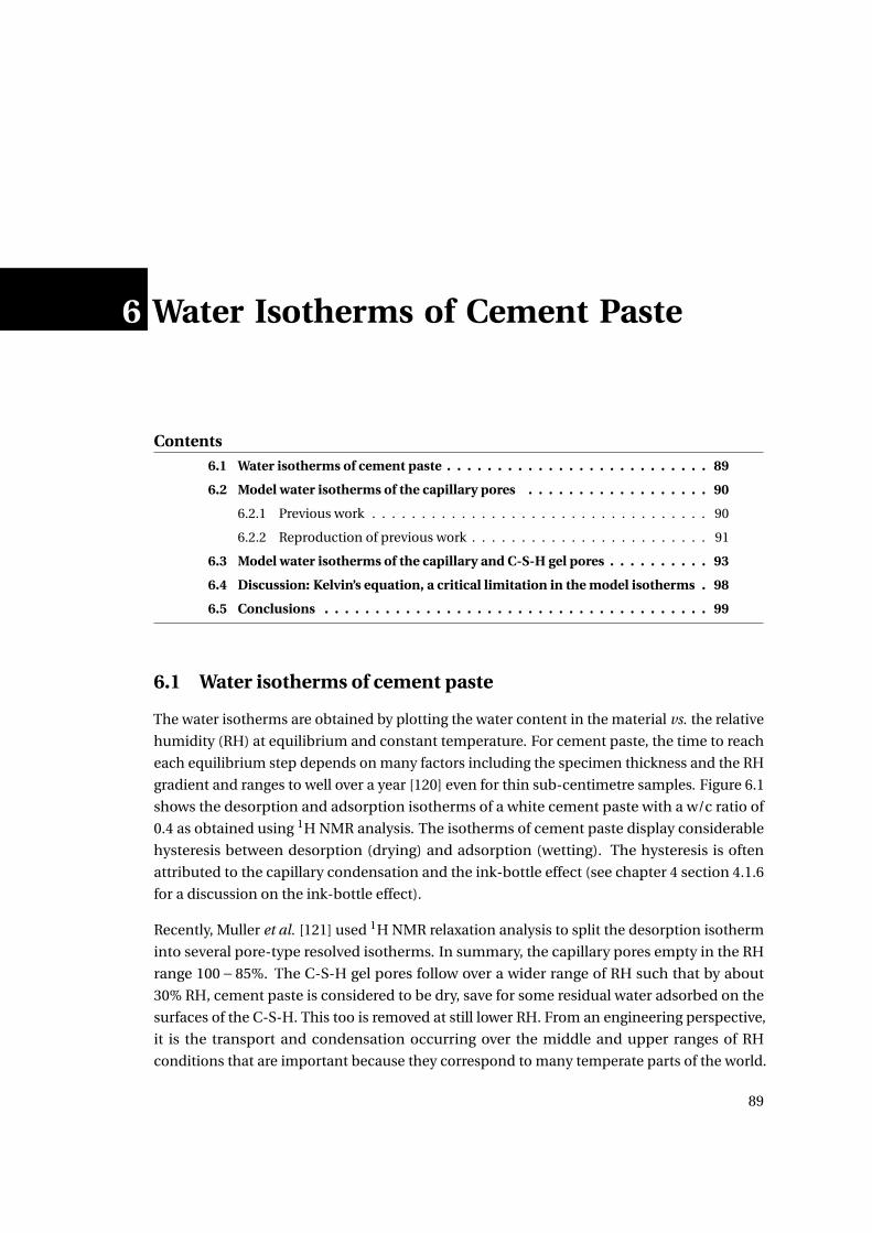
6 Water Isotherms of Cement Paste
Contents
6.1 Water isotherms of cement paste . . . . . . . . . . . . . . . . . . . . . . . . . . 89
6.2 Model water isotherms of the capillary pores . . . . . . . . . . . . . . . . . . 90
6.2.1 Previous work . . . . . . . . . . . . . . . . . . . . . . . . . . . . . . . . . . 90
6.2.2 Reproduction of previous work . . . . . . . . . . . . . . . . . . . . . . . . 91
6.3 Model water isotherms of the capillary and C-S-H gel pores . . . . . . . . . . 93
6.4 Discussion: Kelvin’s equation, a critical limitation in the model isotherms . 98
6.5 Conclusions . . . . . . . . . . . . . . . . . . . . . . . . . . . . . . . . . . . . . . 99
6.1 Water isotherms of cement paste
The water isotherms are obtained by plotting the water content in the material vs. the relative
humidity (RH) at equilibrium and constant temperature. For cement paste, the time to reach
each equilibrium step depends on many factors including the specimen thickness and the RH
gradient and ranges to well over a year [120] even for thin sub-centimetre samples. Figure 6.1
shows the desorption and adsorption isotherms of a white cement paste with a w/c ratio of
0.4 as obtained using 1H NMR analysis. The isotherms of cement paste display considerable
hysteresis between desorption (drying) and adsorption (wetting). The hysteresis is often
attributed to the capillary condensation and the ink-bottle effect (see chapter 4 section 4.1.6
for a discussion on the ink-bottle effect).
Recently, Muller et al. [121] used 1H NMR relaxation analysis to split the desorption isotherm
into several pore-type resolved isotherms. In summary, the capillary pores empty in the RH
range 100−85%. The C-S-H gel pores follow over a wider range of RH such that by about
30% RH, cement paste is considered to be dry, save for some residual water adsorbed on the
surfaces of the C-S-H. This too is removed at still lower RH. From an engineering perspective,
it is the transport and condensation occurring over the middle and upper ranges of RH
conditions that are important because they correspond to many temperate parts of the world.
89
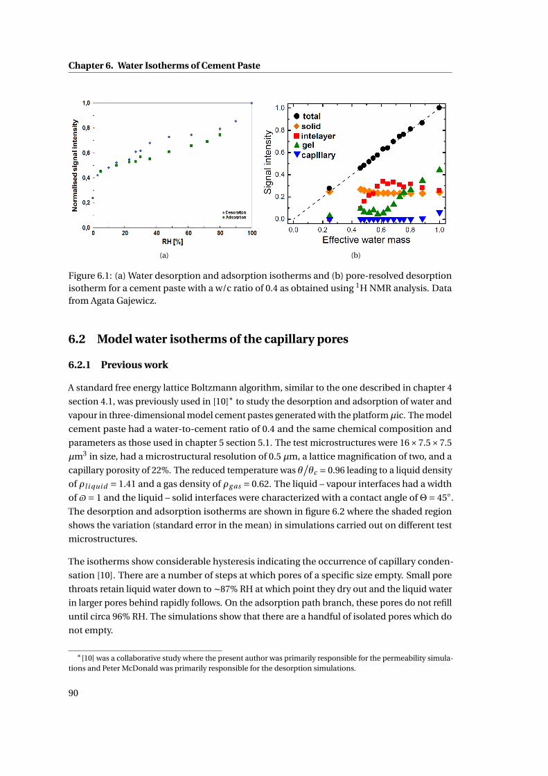
Chapter 6. Water Isotherms of Cement Paste
(a) (b)
Figure 6.1: (a) Water desorption and adsorption isotherms and (b) pore-resolved desorptionisotherm for a cement paste with a w/c ratio of 0.4 as obtained using 1H NMR analysis. Datafrom Agata Gajewicz.
6.2 Model water isotherms of the capillary pores
6.2.1 Previous work
A standard free energy lattice Boltzmann algorithm, similar to the one described in chapter 4
section 4.1, was previously used in [10]∗ to study the desorption and adsorption of water and
vapour in three-dimensional model cement pastes generated with the platformµic. The model
cement paste had a water-to-cement ratio of 0.4 and the same chemical composition and
parameters as those used in chapter 5 section 5.1. The test microstructures were 16×7.5×7.5
µm3 in size, had a microstructural resolution of 0.5 µm, a lattice magnification of two, and a
capillary porosity of 22%. The reduced temperature was θ/θc = 0.96 leading to a liquid density
of ρl i qui d = 1.41 and a gas density of ρg as = 0.62. The liquid – vapour interfaces had a width
of $= 1 and the liquid – solid interfaces were characterized with a contact angle of Θ= 45.
The desorption and adsorption isotherms are shown in figure 6.2 where the shaded region
shows the variation (standard error in the mean) in simulations carried out on different test
microstructures.
The isotherms show considerable hysteresis indicating the occurrence of capillary conden-
sation [10]. There are a number of steps at which pores of a specific size empty. Small pore
throats retain liquid water down to ∼87% RH at which point they dry out and the liquid water
in larger pores behind rapidly follows. On the adsorption path branch, these pores do not refill
until circa 96% RH. The simulations show that there are a handful of isolated pores which do
not empty.
∗[10] was a collaborative study where the present author was primarily responsible for the permeability simula-tions and Peter McDonald was primarily responsible for the desorption simulations.
90
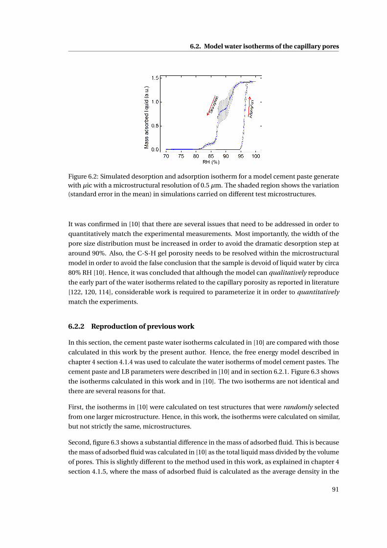
6.2. Model water isotherms of the capillary pores
Figure 6.2: Simulated desorption and adsorption isotherm for a model cement paste generatewith µic with a microstructural resolution of 0.5 µm. The shaded region shows the variation(standard error in the mean) in simulations carried on different test microstructures.
It was confirmed in [10] that there are several issues that need to be addressed in order to
quantitatively match the experimental measurements. Most importantly, the width of the
pore size distribution must be increased in order to avoid the dramatic desorption step at
around 90%. Also, the C-S-H gel porosity needs to be resolved within the microstructural
model in order to avoid the false conclusion that the sample is devoid of liquid water by circa
80% RH [10]. Hence, it was concluded that although the model can qualitatively reproduce
the early part of the water isotherms related to the capillary porosity as reported in literature
[122, 120, 114], considerable work is required to parameterize it in order to quantitatively
match the experiments.
6.2.2 Reproduction of previous work
In this section, the cement paste water isotherms calculated in [10] are compared with those
calculated in this work by the present author. Hence, the free energy model described in
chapter 4 section 4.1.4 was used to calculate the water isotherms of model cement pastes. The
cement paste and LB parameters were described in [10] and in section 6.2.1. Figure 6.3 shows
the isotherms calculated in this work and in [10]. The two isotherms are not identical and
there are several reasons for that.
First, the isotherms in [10] were calculated on test structures that were randomly selected
from one larger microstructure. Hence, in this work, the isotherms were calculated on similar,
but not strictly the same, microstructures.
Second, figure 6.3 shows a substantial difference in the mass of adsorbed fluid. This is because
the mass of adsorbed fluid was calculated in [10] as the total liquid mass divided by the volume
of pores. This is slightly different to the method used in this work, as explained in chapter 4
section 4.1.5, where the mass of adsorbed fluid is calculated as the average density in the
91
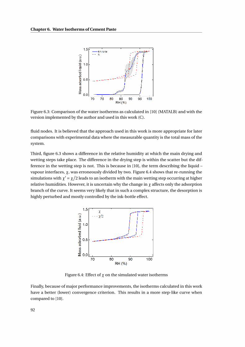
Chapter 6. Water Isotherms of Cement Paste
Figure 6.3: Comparison of the water isotherms as calculated in [10] (MATALB) and with theversion implemented by the author and used in this work (C).
fluid nodes. It is believed that the approach used in this work is more appropriate for later
comparisons with experimental data where the measurable quantity is the total mass of the
system.
Third, figure 6.3 shows a difference in the relative humidity at which the main drying and
wetting steps take place. The difference in the drying step is within the scatter but the dif-
ference in the wetting step is not. This is because in [10], the term describing the liquid –
vapour interfaces, χ, was erroneously divided by two. Figure 6.4 shows that re-running the
simulations with χ′ =χ/2 leads to an isotherm with the main wetting step occurring at higher
relative humidities. However, it is uncertain why the change in χ affects only the adsorption
branch of the curve. It seems very likely that in such a complex structure, the desorption is
highly perturbed and mostly controlled by the ink-bottle effect.
Figure 6.4: Effect of χ on the simulated water isotherms
Finally, because of major performance improvements, the isotherms calculated in this work
have a better (lower) convergence criterion. This results in a more step-like curve when
compared to [10].
92
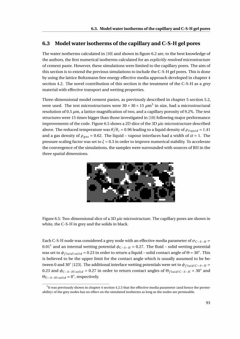
6.3. Model water isotherms of the capillary and C-S-H gel pores
6.3 Model water isotherms of the capillary and C-S-H gel pores
The water isotherms calculated in [10] and shown in figure 6.2 are, to the best knowledge of
the authors, the first numerical isotherms calculated for an explicitly-resolved microstructure
of cement paste. However, these simulations were limited to the capillary pores. The aim of
this section is to extend the previous simulations to include the C-S-H gel pores. This is done
by using the lattice Boltzmann free energy effective media approach developed in chapter 4
section 4.2. The novel contribution of this section is the treatment of the C-S-H as a grey
material with effective transport and wetting properties.
Three-dimensional model cement pastes, as previously described in chapter 5 section 5.2,
were used. The test microstructures were 30× 30× 15 µm3 in size, had a microstructural
resolution of 0.5 µm, a lattice magnification of two, and a capillary porosity of 9.2%. The test
structures were 15 times bigger than those investigated in [10] following major performance
improvements of the code. Figure 6.5 shows a 2D slice of the 3D µic microstructure described
above. The reduced temperature was θ/θc = 0.96 leading to a liquid density of ρl i qui d = 1.41
and a gas density of ρg as = 0.62. The liquid – vapour interfaces had a width of $ = 1. The
pressure scaling factor was set to ξ= 0.3 in order to improve numerical stability. To accelerate
the convergence of the simulations, the samples were surrounded with sources of RH in the
three spatial dimensions.
Figure 6.5: Two-dimensional slice of a 3D µic microstructure. The capillary pores are shown inwhite, the C-S-H in grey and the solids in black.
Each C-S-H node was considered a grey node with an effective media parameter of σC−S−H =0.01† and an internal wetting potential φC−S−H = 0.27. The fluid – solid wetting potential
was set to φ f lui d/sol i d = 0.23 in order to return a liquid – solid contact angle ofΘ= 30. This
is believed to be the upper limit for the contact angle which is usually assumed to be be-
tween 0 and 30 [123]. The additional interface wetting potentials were set to φ f lui d/C−S−H =0.23 and φC−S−H/sol i d = 0.27 in order to return contact angles of Θ f lui d/C−S−H = 30 and
ΘC−S−H/sol i d = 0, respectively.
†It was previously shown in chapter 4 section 4.2.5 that the effective media parameter (and hence the perme-ability) of the grey nodes has no effect on the simulated isotherms as long as the nodes are permeable.
93
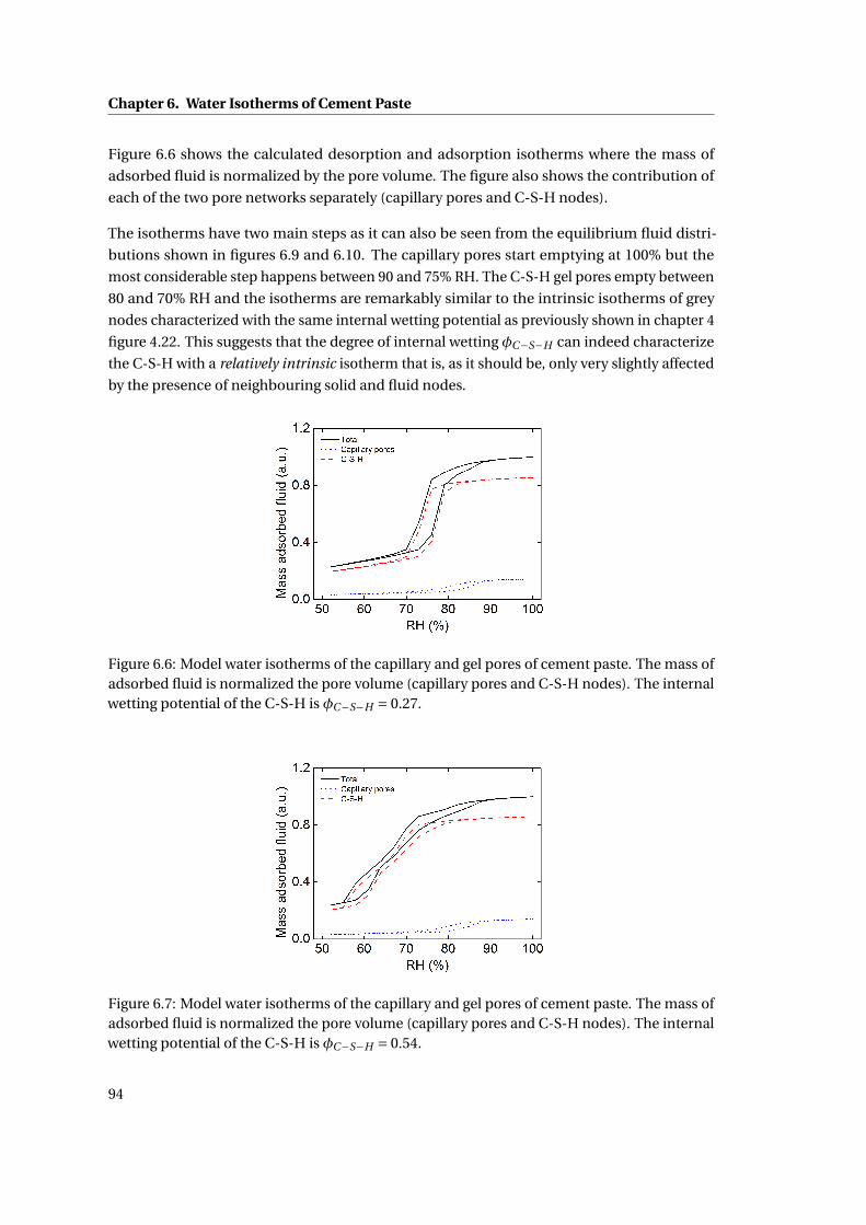
Chapter 6. Water Isotherms of Cement Paste
Figure 6.6 shows the calculated desorption and adsorption isotherms where the mass of
adsorbed fluid is normalized by the pore volume. The figure also shows the contribution of
each of the two pore networks separately (capillary pores and C-S-H nodes).
The isotherms have two main steps as it can also be seen from the equilibrium fluid distri-
butions shown in figures 6.9 and 6.10. The capillary pores start emptying at 100% but the
most considerable step happens between 90 and 75% RH. The C-S-H gel pores empty between
80 and 70% RH and the isotherms are remarkably similar to the intrinsic isotherms of grey
nodes characterized with the same internal wetting potential as previously shown in chapter 4
figure 4.22. This suggests that the degree of internal wetting φC−S−H can indeed characterize
the C-S-H with a relatively intrinsic isotherm that is, as it should be, only very slightly affected
by the presence of neighbouring solid and fluid nodes.
Figure 6.6: Model water isotherms of the capillary and gel pores of cement paste. The mass ofadsorbed fluid is normalized the pore volume (capillary pores and C-S-H nodes). The internalwetting potential of the C-S-H is φC−S−H = 0.27.
Figure 6.7: Model water isotherms of the capillary and gel pores of cement paste. The mass ofadsorbed fluid is normalized the pore volume (capillary pores and C-S-H nodes). The internalwetting potential of the C-S-H is φC−S−H = 0.54.
94
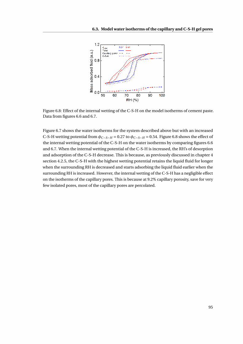
6.3. Model water isotherms of the capillary and C-S-H gel pores
Figure 6.8: Effect of the internal wetting of the C-S-H on the model isotherms of cement paste.Data from figures 6.6 and 6.7.
Figure 6.7 shows the water isotherms for the system described above but with an increased
C-S-H wetting potential from φC−S−H = 0.27 to φC−S−H = 0.54. Figure 6.8 shows the effect of
the internal wetting potential of the C-S-H on the water isotherms by comparing figures 6.6
and 6.7. When the internal wetting potential of the C-S-H is increased, the RH’s of desorption
and adsorption of the C-S-H decrease. This is because, as previously discussed in chapter 4
section 4.2.5, the C-S-H with the highest wetting potential retains the liquid fluid for longer
when the surrounding RH is decreased and starts adsorbing the liquid fluid earlier when the
surrounding RH is increased. However, the internal wetting of the C-S-H has a negligible effect
on the isotherms of the capillary pores. This is because at 9.2% capillary porosity, save for very
few isolated pores, most of the capillary pores are percolated.
95
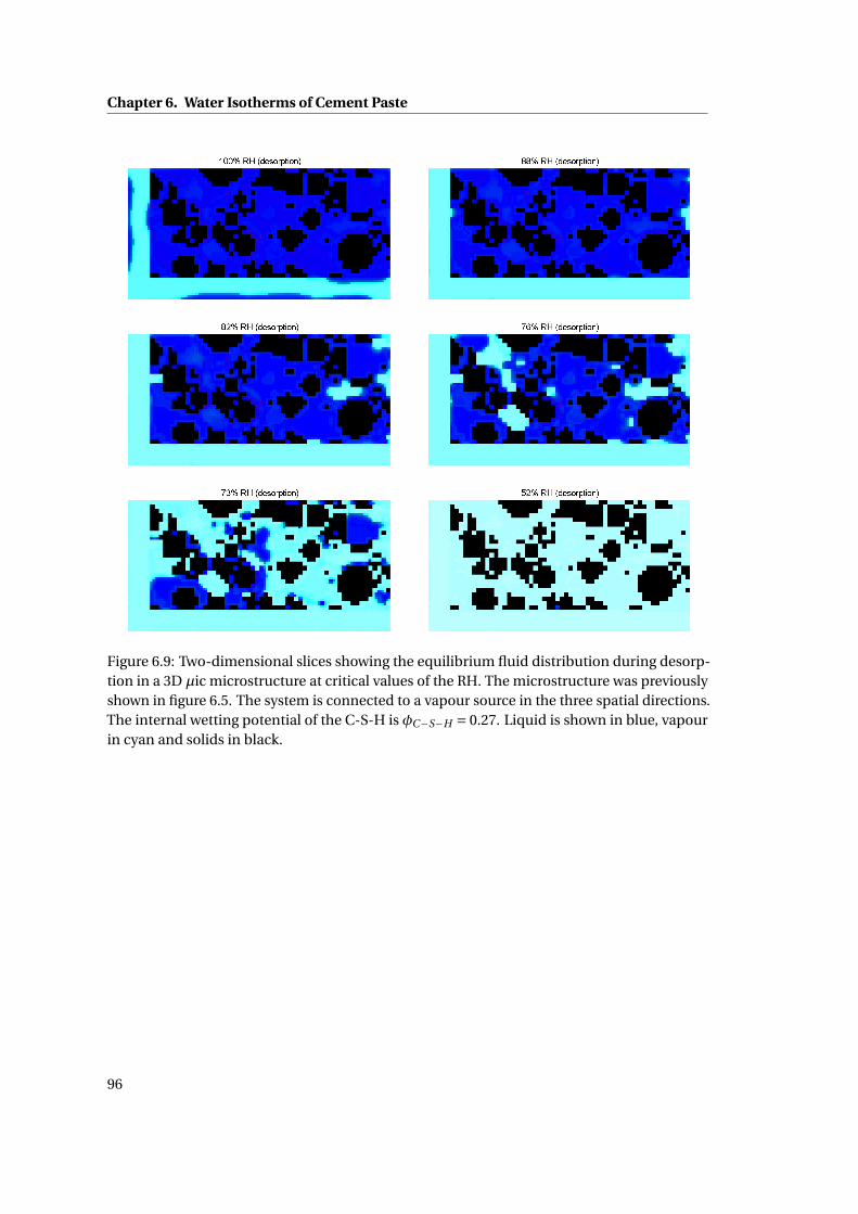
Chapter 6. Water Isotherms of Cement Paste
Figure 6.9: Two-dimensional slices showing the equilibrium fluid distribution during desorp-tion in a 3D µic microstructure at critical values of the RH. The microstructure was previouslyshown in figure 6.5. The system is connected to a vapour source in the three spatial directions.The internal wetting potential of the C-S-H is φC−S−H = 0.27. Liquid is shown in blue, vapourin cyan and solids in black.
96
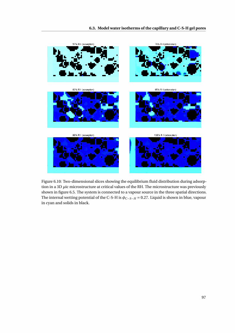
6.3. Model water isotherms of the capillary and C-S-H gel pores
Figure 6.10: Two-dimensional slices showing the equilibrium fluid distribution during adsorp-tion in a 3D µic microstructure at critical values of the RH. The microstructure was previouslyshown in figure 6.5. The system is connected to a vapour source in the three spatial directions.The internal wetting potential of the C-S-H is φC−S−H = 0.27. Liquid is shown in blue, vapourin cyan and solids in black.
97
Chapter 6. Water Isotherms of Cement Paste
6.4 Discussion: Kelvin’s equation, a critical limitation in the model
isotherms
The water isotherms calculated in section 6.3 addressed the limitations that were previously
exposed in [10]. Specifically, the test structures were bigger, had a wider pore size distribution,
and the C-S-H was taken into account via the novel lattice Boltzmann free energy effective
media method. However, there is a further critical problem related to the parametrization of
the LB model with regards to the Kelvin equation (see chapter 4 section 4.1.6 for a discussion
on the Kelvin equation). Taking data from figure 4.14 in section 4.1.6, it is found that in
the LB simulations, a 3D spherical pore with a radius of six lattice units empties at 90.4%
RH. The microstructural resolution of the model cement pastes is ∼0.5 µm and the lattice
magnification is 2. Therefore, in the cement paste microstructures, a pore with a radius of
six lattice units would have a physical radius of 1.5 µm. However, using the Kelvin equation
(equation 4.18) and the following standard experimental parameters:
γ= 0.073 N.m−1
Θ= 30
R = 8.314 J.mol−1K−1
T = 300 K
Tc = 647 K
M∗ = 0.018 m3.mol−1
ρ = 1003 Kg.m−3
it is found that a spherical pore that empties from liquid water at 90.4% RH should have a
physical radius of ∼9 nm. This means that the six lattice units of the LB simulations represent
∼9 nm in terms of physical units and not 0.25 µm as imposed by the resolution and magnifica-
tion of the microstructure. One could think that the discrepancy may arise from the fact that
water at room temperature has a reduced temperature of θ/θc = 300/647 ' 0.47 whereas the
fluid in the LB model was characterized with a reduced temperature of θ/θc = 0.96. However,
further tests revealed that decreasing the simulation temperature does decrease, not increase,
the RH at which the pore emptied (table 6.1).
Table 6.1: RH at which a pore of radius six lattice units empties from liquid water for differentvalues of the reduced simulation temperature.
θ/θc ρl i qui d /ρg as RH(%±0.5%)
0.99 1.5 96.50.96 2.27 90.50.92 3.3 80.5
To the best of the author’s knowledge, the practical problem of linking the spatial dimension
98
6.5. Conclusions
of the structure to the RH of desorption has not been discussed nor solved. At present, it is
unclear how to parameterize the free energy lattice Boltzmann algorithm in order to adjust
the physical size of the lattice unit‡. There are several governing parameters (e.g. contact
angle, interface width) but none of them is sufficient to link the spatial dimension to the
RH of desorption without affecting the physics or the stability of the simulation. Hence, at
present, the only quick-fix consists of magnifying the structure. For the reduced temperature
θ/θc = 0.96, the magnification that is needed in order to adjust the physical resolution is ∼28
times. Unfortunately, this is hopeless from a computational point of view.
6.5 Conclusions
In this chapter, a novel lattice Boltzmann algorithm was used to model the desorption and
adsorption of water in cement paste. The novelties of the numerical model were previously
described in chapter 4 section 4.2.7. From the cement paste perspective, this chapter pre-
sented, to the best knowledge of the author, the first numerical isotherms of cement paste
that is based on an explicitly-resolved microstructure and includes the contribution of both
capillary and C-S-H gel pores.
At present, the lattice spacing in the simulations is on the order of few nanometres and cannot
be matched to the characteristic dimensions of the cement paste model microstructures.
Hence, the algorithm was used to study qualitatively the effect of the inclusion of the gel pores
on the calculated isotherms of cement paste. The algorithm was also used to test hypotheses
like the ink-bottle effect. Thus, unlike chapter 5, this chapter does not end with a quantitative
comparison of the model with experiments. However, the model is only one step away from
such comparisons.
‡This was not the case for the permeability simulations shown in chapter 5 where the simulation and physicalunits were fully controlled.
99

7 Conclusions
Contents
7.1 Main findings . . . . . . . . . . . . . . . . . . . . . . . . . . . . . . . . . . . . . 101
7.2 Outlook . . . . . . . . . . . . . . . . . . . . . . . . . . . . . . . . . . . . . . . . . 102
7.2.1 Water isotherms of cement paste . . . . . . . . . . . . . . . . . . . . . . . 103
7.2.2 Experimental validation . . . . . . . . . . . . . . . . . . . . . . . . . . . . 103
7.2.3 Microstructural resolution . . . . . . . . . . . . . . . . . . . . . . . . . . 104
7.2.4 Downscaling . . . . . . . . . . . . . . . . . . . . . . . . . . . . . . . . . . . 104
7.2.5 Upscaling . . . . . . . . . . . . . . . . . . . . . . . . . . . . . . . . . . . . 104
7.1 Main findings
The objective of this thesis was to develop a model that can predict the permeability of cement
paste based on an explicit microstructure. To achieve this, three-dimensional model mi-
crostructures were generated using the platform µic which allows the simulation of resolution-
free structures based on, amongst others, input laws for reactions, kinetics and nucleation.
The lattice Boltzmann (LB) method was selected for solving the equations of flow because of
its ability to handle solid boundaries in complex porous media like cement paste.
Two main lattice Boltzmann permeability models were developed. The first model was mo-
tivated by the general consensus that the permeability is governed by the flow through the
fully saturated capillary pores. Hence, a relatively standard LB model was developed and used
to compute the flow in fully saturated microstructures where the calcium silicate hydrate
(C-S-H) was treated as an impermeable solid. In this study, the main parameters were the
water-to-cement ratio, the degree of hydration and the capillary porosity. The calculated per-
meabilities were several orders of magnitude larger than most experimental measurements. At
first, this discrepancy was associated with the limited spatial resolution in the microstructures
and diagonal leaks in the LB method. However, during the comparison of the results with
experimental data, a large unexplained scatter in literature was discovered.
101
Chapter 7. Conclusions
A careful study of the available experimental data suggested that the reason behind this scatter
might be the variation in the degree of water saturation of the samples caused by different
conditioning procedures. Consequently, a second LB model was developed where, in addition
to the improved resolution, the capillary pores were not fully saturated. However, the problem
that arose was that at middle to low degrees of water saturation, the water-filled capillary pores
would depercolate and the permeability would become zero. Hence, the gel pores of the C-S-H
had to be considered in the flow simulation. The issue is that the porous nature of the C-S-H
is uncertain and is not revealed by microstructural models. Thus, it was decided to consider
the C-S-H as an effective medium and to characterize it with an effective permeability. In this
study, the main parameters were the degree of water saturation of the capillary porosity and
the intrinsic permeability of the C-S-H.
The simulation of apparent permeability at different degrees of water saturation provided
a very plausible explanation for the enormous range of experimental results (10−16 −10−22
m2). It was found that when the capillary porosity was completely saturated with a fluid
(either water or gas), the calculated intrinsic permeability was in good agreement with mea-
surements of gas permeability on dried samples (10−16 −10−17 m2). However, as the water
saturation was reduced, the calculated apparent water permeability decreased and span the
full range of experimentally measured values (10−16 −10−22 m2). It was concluded that the
degree of capillary water saturation is very likely to be the cause for variation in experimental
permeability measurements. Based on the modelling results and the analysis of the available
experimental data, it was suggested that most experimental measurements with water are
not conducted on fully saturated samples. In such experiments, the presence of air voids in
nominally water-saturated samples dramatically lowers their apparent permeability.
It was further concluded that the role of the weakly-permeable C-S-H, omitted in earlier
modelling studies, is critical for determining the water permeability at low capillary saturation
or porosity. The role of the C-S-H becomes more important as the saturated capillary porosity
starts to depercolate. This is seen by comparing the results with previous LB permeability
simulations that treated the C-S-H as an impermeable solid. In those calculations, as the
capillary porosity decreased by increasing the degree of hydration, the permeability decreased
monotonically and catastrophically close the percolation threshold, below which it could not
be calculated accurately. In the effective media model, however, an asymptotic approach
towards a plateau permeability dictated by the C-S-H is seen.
7.2 Outlook
This thesis provided insights on the link between the microstructure and the permeability of
cement paste. There are several possible ways to continue and improve on this work.
102
7.2. Outlook
7.2.1 Water isotherms of cement paste
A multi-phase model of non-ideal fluids is required to simulate the desorption and adsorption
of liquid water and vapour in partially-saturated samples. The development of a multi-phase
LB model was already started in chapter 4. Preliminary results were shown in chapter 6
section 6.2 where the model was used to calculate the water isotherms of the capillary pores
of model cement paste. The calculated isotherms were narrow, as expected from the pore
size distribution. Hence, it was decided to include the smaller C-S-H gel pores with a novel
effective media approach, similar to the one used in the permeability simulations in chapter 5
section 5.2. To do so, the effective media approach was extended to include, in addition
to the transport properties, the wetting properties of the C-S-H. This model was applied to
simulate the water isotherms of the capillary and C-S-H gel pores of cement paste in chapter 6
section 6.3. In agreement with experiments, the calculated isotherms have two main steps,
the first corresponding to the capillary pores and the second to the smaller gel pores.
However, at present, the model still has one major limitation. The lattice spacing in the
simulations is on the order of few nanometers and it is unclear how to scale it up to match the
characteristic size of the capillary pores. Hence, the model can be used to simulate phenomena
that are either on the nanometre scale (characteristic pore radii of ∼ 1 to 20 nm), or that are
scale independent (e.g. phase separation, contact angle). Unfortunately, at present, the model
cannot be used to predict in a quantitative manner phenomena that are scale dependent
and have characteristic size larger than few nanometres, like the desorption in cement paste.
However, the developed model is only one parametrization step away from such simulations.
Afterwards, the calculated water isotherms can be compared quantitatively with experimental
data.
7.2.2 Experimental validation
The main result of the thesis is a hypothesis that links the permeability to the degree of capillary
saturation of cement paste. The comparison between the modelling results and experimental
data was done on the basis of matching the degree of saturation in the model microstructures
with the probable degree of saturation in the experiments. The latter was estimated from
the conditioning procedure of the samples. A well-thought-out experiment would be very
valuable to validate the hypothesis regarding saturation in a more definitive manner. The
problem is that it is very hard to ensure full water saturation throughout the curing of the
sample and the permeability experiment. A promising approach may consist of using the
beam bending method on very thin samples that are cured underwater immediately after
mixing. The dilemma in this case is that the effective water-to-cement ratio of the paste will
increase as the water is drawn into the forming air voids during underwater curing. In this
case, nuclear magnetic resonance relaxation analysis could be used to check if the additional
water is uniformly distributed throughout the sample.
103
Chapter 7. Conclusions
7.2.3 Microstructural resolution
The dependency of the permeability on the microstructural resolution was a major issue in
chapter 5 section 5.1. This is because treating the C-S-H as an impermeable solid makes
the percolation of the pore network, and thus the permeability, critically dependent on the
resolution of the model microstructures. This issue was largely addressed in chapter 5 sec-
tion 5.2 where in addition to a slightly improved resolution, the C-S-H was treated as a weakly-
permeable material. These improvements decreased the dependency of the percolation of the
pore network on the microstructural resolution. Hence, the dependency of the permeability
on the microstructural resolution was also decreased. However, it would be interesting to
improve the performance of the code to take full advantage of the resolution-free nature of
the hydration model µic. Moreover, an increased computing power can be used to run the
simulations with a higher lattice magnification and guarantee a better numerical accuracy.
7.2.4 Downscaling
The C-S-H gel pores have to be taken into account to accurately predict the transport properties
of cement paste. In this work, this was done with an effective media approach where the
C-S-H was assigned intrinsic transport and wetting properties. The primary motivation for
this choice was the unavailability of a three-dimensional C-S-H structure. However, there is a
lack of readily available data for the C-S-H transport properties as well. In the permeability
simulations, the C-S-H was characterized with an intrinsic permeability of κC−S−H = 7×10⁻²³
m2. This is the only value that was found in literature and it is extracted from the work of
Powers [118] where he says that ”measurements show that the coefficient of permeability of
the gel itself is about 7×10⁻¹¹ darcys”. However, it is unclear how these measurements were
made. Hence, in chapter 5 section 5.2.4, the permeability of the C-S-H was increased and
decreased by a factor 10. It was found that the permeability of the C-S-H has a non-linear
effect on the permeability of cement paste. In future work, it may be possible to decide the
intrinsic transport and wetting properties of the C-S-H based on newly available experimental
data or atomistic simulations.
7.2.5 Upscaling
The simulations in this work were carried out on a cement paste representative elementary
volume (REV) of (100 µm)3. This relatively small size is a good starting point to understand the
link between the microstructure and transport properties. However, as important as it may be
to understand the fundamentals at the nano- and micro-scales, the ultimate goal is to improve
the properties at the macroscopic scale of concrete structures where the REV is on the order of
cubic centimetres. Fortunately, the developed lattice Boltzmann models are very appropriate
for such upscaling. In particular, the simulation of the flow is easier and less prone to errors
in concrete structures because their permeability is several orders of magnitude larger than
that of cement paste. Moreover, the LB models that incorporate effective media are appealing
104

7.2. Outlook
to use in a hierarchial manner. In this thesis, the effective media lattice Boltzmann model
was used to simulate the flow in the capillary pores while treating the C-S-H as an effective
medium of known permeability. In future work, the model could be used to calculate the
permeability of concrete where the flow is solved in the micro-cracks and interfacial transition
zones while treating the bulk cement paste as an effective medium of known permeability, as
calculated in this work.
105

A MRT Collision Operator
The multi-relaxation-time collision operator is implemented in the hydraulic modes of the
problem instead of the space of discrete velocities. The first term of the RHS of equation 3.2
becomes [63]:
Q∑j=1
Si j
(f j (r , t )− f eq
j (r , t ))=−M−1 ·S · (m (r , t )−meq (r , t )
)(A.1)
where M is a 19×19 transformation matrix and S is the corresponding diagonal relaxation
matrix. The distributions functions are linked with the hydraulic modes via the transformation
matrix M with:
m = M · f (A.2)
f = M−1 ·m (A.3)
The diagonal relaxation matrix is:
S = di ag (0, s2, s3,0, s5,0, s5,0, s5, s10, s11, s10, s11, s14, s14, s14, s17, s17, s17) (A.4)
and the kinematic viscosity is calculated with:
υ= c2s (s10 − ∆t
2) (A.5)
= c2s (s14 − ∆t
2) (A.6)
107
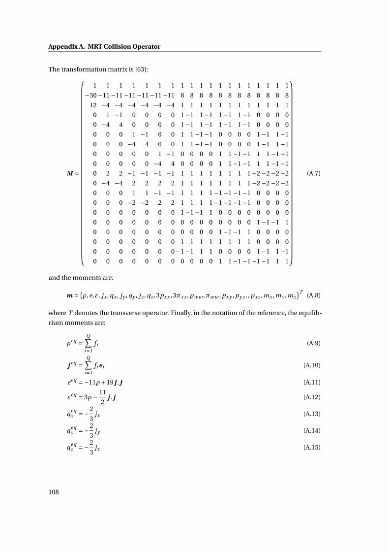
Appendix A. MRT Collision Operator
The transformation matrix is [63]:
M =
1 1 1 1 1 1 1 1 1 1 1 1 1 1 1 1 1 1 1
−30 −11 −11 −11 −11 −11 −11 8 8 8 8 8 8 8 8 8 8 8 8
12 −4 −4 −4 −4 −4 −4 1 1 1 1 1 1 1 1 1 1 1 1
0 1 −1 0 0 0 0 1 −1 1 −1 1 −1 1 −1 0 0 0 0
0 −4 4 0 0 0 0 1 −1 1 −1 1 −1 1 −1 0 0 0 0
0 0 0 1 −1 0 0 1 1 −1 −1 0 0 0 0 1 −1 1 −1
0 0 0 −4 4 0 0 1 1 −1 −1 0 0 0 0 1 −1 1 −1
0 0 0 0 0 1 −1 0 0 0 0 1 1 −1 −1 1 1 −1 −1
0 0 0 0 0 −4 4 0 0 0 0 1 1 −1 −1 1 1 −1 −1
0 2 2 −1 −1 −1 −1 1 1 1 1 1 1 1 1 −2 −2 −2 −2
0 −4 −4 2 2 2 2 1 1 1 1 1 1 1 1 −2 −2 −2 −2
0 0 0 1 1 −1 −1 1 1 1 1 −1 −1 −1 −1 0 0 0 0
0 0 0 −2 −2 2 2 1 1 1 1 −1 −1 −1 −1 0 0 0 0
0 0 0 0 0 0 0 1 −1 −1 1 0 0 0 0 0 0 0 0
0 0 0 0 0 0 0 0 0 0 0 0 0 0 0 1 −1 −1 1
0 0 0 0 0 0 0 0 0 0 0 1 −1 −1 1 0 0 0 0
0 0 0 0 0 0 0 1 −1 1 −1 −1 1 −1 1 0 0 0 0
0 0 0 0 0 0 0 −1 −1 1 1 0 0 0 0 1 −1 1 −1
0 0 0 0 0 0 0 0 0 0 0 1 1 −1 −1 −1 −1 1 1
(A.7)
and the moments are:
m = (ρ,e,ε, jx , qx , jy , qy , jz , qz ,3pxx ,3πxx , pw w ,πw w , px y , py z , , pxz ,mx ,my ,mz
)T (A.8)
where T denotes the transverse operator. Finally, in the notation of the reference, the equilib-
rium moments are:
ρeq =Q∑
i=1fi (A.9)
j eq =Q∑
i=1fi ei (A.10)
eeq =−11ρ+19 j . j (A.11)
εeq = 3ρ− 11
2j . j (A.12)
qeqx =−2
3jx (A.13)
qeqy =−2
3jy (A.14)
qeqz =−2
3jz (A.15)
108
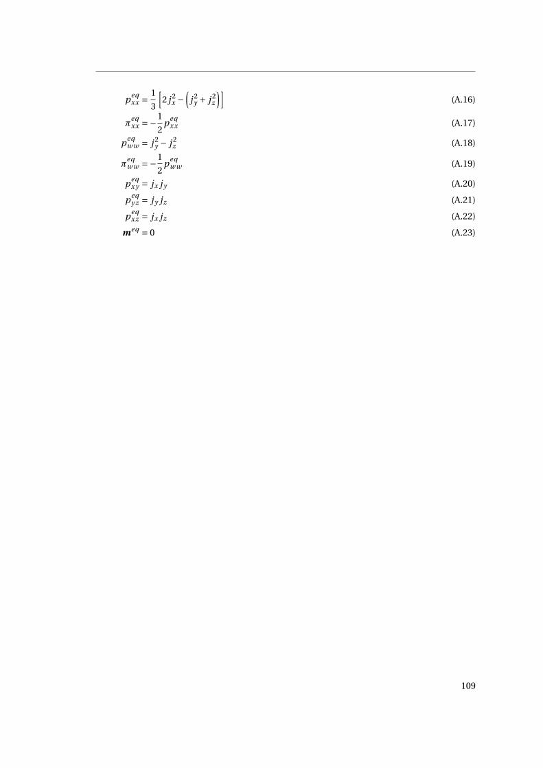
peqxx = 1
3
[2 j 2
x −(
j 2y + j 2
z
)](A.16)
πeqxx =−1
2peq
xx (A.17)
peqw w = j 2
y − j 2z (A.18)
πeqw w =−1
2peq
w w (A.19)
peqx y = jx jy (A.20)
peqy z = jy jz (A.21)
peqxz = jx jz (A.22)
meq = 0 (A.23)
109

B Pressure Boundary Conditions
As discussed in chapter 3 section 3.1.3, pressure boundary conditions can be set in isothermal
lattice Boltzmann simulations by taking advantage of the equation of state that links the
pressure P to the density ρ with P = c2s ρ.
For the following D3Q19 vector base:i
ei x
ei y
ei z
=
1 2 3 4 5 6 7 8 9 10 11 12 13 14 15 16 17 18 19
0 1 −1 0 0 0 0 1 1 1 1 −1 −1 −1 −1 0 0 0 0
0 0 0 1 −1 0 0 1 −1 0 0 1 −1 0 0 1 1 −1 −1
0 0 0 0 0 1 −1 0 0 1 −1 0 0 1 −1 1 −1 1 −1
(B.1)
the density and momentum equations (equations 3.3 and 3.4) are:
ρ = f1 + f2 + f3 + f4 + f5 + f6 + f7 + f8 + f9 + f10 (B.2)
+ f11 + f12 + f13 + f14 + f15 + f16 + f17 + f18 + f19
ρux = f2 + f8 + f9 + f10 + f11 −(
f3 + f12 + f13 + f14 + f15)
(B.3)
ρuy = f4 + f8 + f12 + f16 + f17 −(
f5 + f9 + f14 + f18 + f19)
(B.4)
ρuz = f6 + f10 + f14 + f16 + f18 −(
f7 + f11 + f15 + f16 + f18)
(B.5)
As discussed in section 3.1.3, it is possible to fix only three of the four macroscopic variables. If
the density is set to ρ = ρi nlet and the velocities to uy = uz = 0, the set of equations become:
f2 + f8 + f9 + f10 + f11 = ρi nlet (B.6)
− (f1 + f3 + f4 + f5 + f6 + f7 + f12 + f13 + f14 + f15 + f16 + f17 + f18 + f19
)f2 + f8 + f9 + f10 + f11 = ρi nlet ux (B.7)
− (f3 + f12 + f13 + f14 + f15
)In order to obtain the five unknown components
f2, f8, f9, f10, f11
, three additional equations
are needed. These equations can be obtained by assuming that the half-way bounce-back
111
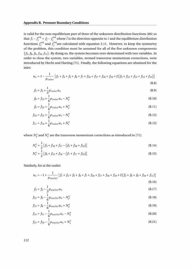
Appendix B. Pressure Boundary Conditions
is valid for the non-equilibrium part of three of the unknown distribution functions [66] so
that fi − f eqi = f i − f eq
iwhere i is the direction opposite to i and the equilibrium distribution
functions f eqi and f eq
iare calculated with equation 3.11. However, to keep the symmetry
of the problem, this condition must be assumed for all of the five unknown componentsf2, f8, f9, f10, f11
. By doing so, the system becomes over-determined with two variables. In
order to close the system, two variables, termed transverse momentum corrections, were
introduced by Hecht and Harting [71]. Finally, the following equations are obtained for the
inlet:
ux = 1− 1
ρi nlet
[f1 + f4 + f5 + f6 + f7 + f16 + f17 + f18 + f19 +2
(f3 + f12 + f13 + f14 + f15
)](B.8)
f2 = f3 + 1
3ρi nlet ux (B.9)
f8 = f13 + 1
6ρi nlet ux −N x
y (B.10)
f9 = f12 + 1
6ρi nlet ux +N x
y (B.11)
f10 = f15 + 1
6ρi nlet ux −N x
z (B.12)
f11 = f14 + 1
6ρi nlet ux +N x
z (B.13)
where N xy and N x
z are the transverse momentum corrections as introduced in [71]:
N xy = 1
2
[f4 + f16 + f17 −
(f5 + f18 + f19
)](B.14)
N xz = 1
2
[f6 + f12 + f16 −
(f7 + f17 + f19
)](B.15)
Similarly, for at the outlet:
ux =−1+ 1
ρoutlet
[f1 + f4 + f5 + f6 + f7 + f16 + f17 + f18 + f19 +2
(f2 + f8 + f9 + f10 + f11
)](B.16)
f3 = f2 − 1
3ρoutlet ux (B.17)
f12 = f9 − 1
6ρoutlet ux −N x
y (B.18)
f13 = f8 − 1
6ρoutlet ux +N x
y (B.19)
f14 = f11 − 1
6ρoutlet ux −N x
z (B.20)
f15 = f10 − 1
6ρoutlet ux +N x
z (B.21)
112
C Effective permeability
In this appendix, the analytical expression given in equation 3.32 that relates the effective
media parameter to the intrinsic permeability of a grey node is derived∗. To do so, the
three-dimensional lattice is projected onto a one-dimensional lattice with three velocities:
a stationary velocity e0, a velocity in the positive direction e+, and a velocity in the negative
direction e−. The equations governing the equilibrium fluid densities become:
f eq0 = ρ
(2
3−u2
)(C.1)
f eq+ = 1
6ρ
(1+3u +3u2) (C.2)
f eq− = 1
6ρ
(1−3u +3u2) (C.3)
The stationary fluid packed density is constant under steady-state conditions. Consequently:
f0 = ρ(
2
3−u2
)(C.4)
f+2 = (1−σ) f+1 +σ f−1 (C.5)
f−1 = (1−σ) f−2 +σ f+2 (C.6)
where the additional subscripts refer to the fluid packets for two neighbouring nodes 1 and 2.
By introducing the following variables:
p = f++ f− = ρ− f0 (C.7)
m = f+− f− = ρu (C.8)
We obtain:
p2 +m2 = p1 + (1−2σ)m1 (C.9)
p1 −m1 = p2 − (1−2σ)m2 (C.10)
∗The derivation is largely inspired by the work of Walsh et al. [91].
113
Appendix C. Effective permeability
Combining equations C.1, C.9 and C.10 yeilds an expression for the change in p across a
one-dimensional lattice comprising N +1 nodes numbered from 0 to N :
∆p = ρ0
(1
3+u2
0
)−ρN
(1
3+u2
N
)= 2σρ0u0N (C.11)
Equation C.11 can be written under the form:
u20 +
2σρN N
ρ0 −ρNu0 − ρN
3ρ0= 0 (C.12)
Thus,
u0 =− σρN N
ρ0 −ρN+
√(σρN N
ρ0 −ρN
)2
+ ρN
3ρ0
' ∆ρ
6σρ0N(C.13)
where the change in density, ∆ρ = ρ0 −ρN , is related to the pressure drop ∆P across the lattice
by:
∆P = 1
3∆ρ (C.14)
Finally, the permeability κ of a grey node of effective media parameter σ can be obtained from
equations 3.29, 2.1, C.13 and C.14:
κ= (1−σ)υ
2σ(C.15)
114
D Mathematical Operators
The gradient and Laplacian stencils can be calculated with:
∂x =
0 0 0
−B 0 B
0 0 0
,
−B 0 B
−A 0 A
−B 0 B
,
0 0 0
−B 0 B
0 0 0
(D.1)
and
∇2 =
0 D 0
D C D
0 D 0
,
D C D
C E C
D C D
,
0 D 0
D C D
0 D 0
(D.2)
where E =−6C −12D, 2A+8B = 1 and C +4D = 1 [101]. The left, middle, and right matrices
show slices of the stencils for ei = (0,0,−1), ei = (0,0,0) and ei = (0,0,1), respectively. The
coefficients A,B ,C and D can be tuned to reduce the spurious velocities at equilibrium. Their
values are chosen following the work of Pooley and Furtado [101] so that: A = 16 ,B = 1
12 ,C =13 ,D = 1
6 and E = −4. The parameters ωp,t ,αα,αβi can be adjusted to reduce the spurious
velocities as well and their values can be found in [101].
In the numerical algorithm, the following expressions were used for the bulk nodes:
∂xρ(x,y,z) =ρ(x+1,y,z) −ρ(x−1,y,z)
6
+ ρ(x+1,y−1,z) +ρ(x+1,y+1,z) +ρ(x+1,y,z−1) +ρ(x+1,y,z+1)
12
− ρ(x−1,y−1,z) +ρ(x−1,y+1,z) +ρ(x−1,y,z−1) +ρ(x−1,y,z+1)
12(D.3)
115
Appendix D. Mathematical Operators
∂yρ(x,y,z) =ρ(x,y+1,z) −ρ(x,y−1,z)
6
+ ρ(x+1,y+1,z) +ρ(x−1,y+1,z) +ρ(x,y+1,z−1) +ρ(x,y+1,z+1)
12
− ρ(x+1,y−1,z) +ρ(x−1,y−1,z) +ρ(x,y−1,z−1) +ρ(x,y−1,z+1)
12(D.4)
∂zρ(x,y,z) =ρ(x,y,z+1) −ρ(x,y,z−1)
6
+ ρ(x+1,y,z+1) +ρ(x−1,y,z+1) +ρ(x,y+1,z+1) +ρ(x,y−1,z+1)
12
− ρ(x+1,y,z−1) +ρ(x−1,y,z−1) +ρ(x,y+1,z−1) +ρ(x,y−1,z−1)
12(D.5)
and
∇2ρ(x,y,z) =ρ(x+1,y,z) +ρ(x−1,y,z) +ρ(x,y+1,z) +ρ(x,y−1,z) +ρ(x,y,z+1) +ρ(x,y,z−1)
3
+ ρ(x+1,y−1,z) +ρ(x−1,y−1,z) +ρ(x+1,y+1,z) +ρ(x−1,y+1,z) +ρ(x+1,y,z−1) +ρ(x−1,y,z−1)
6
+ ρ(x+1,y,z+1) +ρ(x−1,y,z+1) +ρ(x,y+1,z−1) +ρ(x,y−1,z−1) +ρ(x,y+1,z+1) +ρ(x,y−1,z+1)
6
−4ρ(x,y,z) (D.6)
On surface nodes near the solid boundaries, the following expressions were used:
∂xρ(x,y,z) = 1
2
[ρ′σ(x+1,y,z) +ρ(x+1,y,z)
[1−σ(x+1,y,z)
]−ρ′σ(x−1,y,z) −ρ(x−1,y,z)
[1−σ(x−1,y,z)
]](D.7)
∂yρ(x,y,z) = 1
2
[ρ′σ(x,y+1,z) +ρ(x,y+1,z)
[1−σ(x,y+1,z)
]−ρ′σ(x,y−1,z) −ρ(x,y−1,z)
[1−σ(x,y−1,z)
]](D.8)
∂yρ(x,y,z) = 1
2
[ρ′σ(x,y,z+1) +ρ(x,y,z+1)
[1−σ(x,y,z+1)
]−ρ′σ(x,y,z−1) −ρ(x,y,z−1)
[1−σ(x,y,z−1)
]](D.9)
116
and
∇2ρ(x,y,z) =ρ′[σ(x+1,y,z) +σ(x−1,y,z) +σ(x,y+1,z) +σ(x,y−1,z) +σ(x,y,z+1) +σ(x,y,z−1)
]+ρ(x+1,y,z)
[1−σ(x+1,y,z)
]+ρ(x−1,y,z)[1−σ(x−1,y,z)
]+ρ(x,y+1,z)
[1−σ(x,y+1,z)
]+ρ(x,y−1,z)[1−σ(x,y−1,z)
]+ρ(x,y,z+1)
[1−σ(x,y,z+1)
]+ρ(x,y,z−1)[1−σ(x,y,z−1)
]−6ρ(x,y,z)
[1−σ(x,y,z)
](D.10)
where
σ(x,y,z) =
0 if (x,y,z) is a fluid node
1 if (x,y,z) is a solid node(D.11)
ρ′ = ρ(x,y,z)[1−σ(x,y,z)
]+φ (D.12)
and φ is the wetting potential.
117

Bibliography
[1] http://www.wbcsdcement.org.
[2] K. L. Scrivener, A. K. Crumbie, P. Laugesen, The interfacial transition zone (itz) between
cement paste and aggregate in concrete, Interface Science 12 (2004) 411–421.
[3] A. C. A. Muller, K. L. Scrivener, A. M. Gajewicz, P. J. McDonald, Densification of c-s-h
measured by 1h nmr relaxometry, Journal of Physical Chemistry C 117 (2013) 403–412.
[4] H. Wong, M. Zobel, N. Buenfeld, R. Zimmerman, Influence of the interfacial transition
zone and microcracking on the diffusivity, permeability and sorptivity of cement-based
materials after drying, Magazine of Concrete Research 61 (2009) 571 –589.
[5] H. Darcy, Les Fontaines Publiques de la Ville de Dijon, Dalmont, Paris, 1856.
[6] B. Ferreol, D. H. Rothman, Lattice-boltzmann simulations of flow through fontainebleau
sandstone, Transport in Porous Media 20 (1995) 3–20.
[7] Q. Kang, D. Zhang, S. Chen, X. He, Lattice boltzmann simulation of chemical dissolution
in porous media, Physical Review E 65 (2002) 036318.
[8] M. A. Van Doormaal, J. G. Pharoah, Determination of permeability in fibrous porous me-
dia using the lattice boltzmann method with application to pem fuel cells, International
journal for numerical methods in fluids 59 (2009) 75–89.
[9] E. J. Garboczi, D. P. Bentz, The effect of statistical fluctuation, finite size error, and
digital resolution on the phase percolation and transport properties of the nist cement
hydration model, Cement and Concrete Research 31 (2001) 1501–1514.
[10] M. Zalzale, P. J. McDonald, Lattice boltzmann simulations of the permeability and
capillary adsorption of cement model microstructures, Cement and Concrete Research
42 (2012) 1601–1610.
[11] M. Zhang, G. Ye, K. van Breugel, Modeling of ionic diffusivity in non-saturated cement-
based materials using lattice boltzmann method, Cement and Concrete Research 42
(2012) 1524 – 1533.
119
Bibliography
[12] M. Zhang, G. Ye, K. v. Breugel, Microstructure-based modeling of permeability of ce-
mentitious materials using multiple-relaxation-time lattice boltzmann method, Com-
putational Materials Science 68 (2013) 142–151.
[13] M. Zalzale, P. J. McDonald, K. L. Scrivener, A 3d lattice boltzmann effective media study:
understanding the role of c-s-h and water saturation on the permeability of cement
paste, Modelling and Simulation in Materials Science and Engineering 21 (2013) 085016.
[14] R. J.-M. Pellenq, A. Kushima, R. Shahsavari, K. J. Van Vliet, M. J. Buehler, S. Yip, F.-J. Ulm,
A realistic molecular model of cement hydrates, Proceedings of the National Academy
of Sciences 106 (2009) 16102–16107.
[15] S. Galmarini, A. Aimable, N. Ruffray, P. Bowen, Changes in portlandite morphology with
solvent composition: Atomistic simulations and experiment, Cement and Concrete
Research 41 (2011) 1330 – 1338, conferences Special: Cement Hydration Kinetics and
Modeling, Quebec City, 2009; CONMOD10, Lausanne, 2010.
[16] C. Pignat, P. Navi, K. L. Scrivener, Simulation of cement paste microstructure hydration,
pore space characterization and permeability determination, Materials and Structures
38 (2005) 459–466.
[17] M. Koster, J. Hannawald, W. Brameshuber, Simulation of water permeability and water
vapor diffusion through hardened cement paste, Computational Mechanics 37 (2006)
163–172.
[18] G. Ye, P. Lura, K. van Breugel, Modelling of water permeability in cementitious materials,
Materials and Structures 39 (2006) 877–885.
[19] T. C. Powers, L. E. Copeland, J. C. Hayes, H. M. Mann, Permeability of portland cement
paste (1955).
[20] B. K. Nyame, J. M. Illston, Relationships between permeability and pore structure of
hardened cement paste, Magazine of Concrete Research 33 (1981) 139–146.
[21] N. Banthia, S. Mindess, Water permeability of cement paste, Cement and Concrete
Research 19 (1989) 727–736.
[22] G. Ye, Percolation of capillary pores in hardening cement pastes, Cement and Concrete
Research 35 (2005) 167–176.
[23] W. Vichit-Vadakan, G. W. Scherer, Measuring permeability and stress relaxation of young
cement paste by beam bending, Cement and Concrete Research 33 (2003) 1925–1932.
[24] H. Ai, J. F. Young, G. W. Scherer, Thermal expansion kinetics: Method to measure perme-
ability of cementitious materials: Ii, application to hardened cement pastes, Journal of
the American Ceramic Society 84 (2001) 385–91.
120
Bibliography
[25] W. Vichit-Vadakan, G. Scherer, Measuring permeability of rigid materials by a beam-
bending method: Iii, cement paste, Journal of the American Ceramic Society 85 (2002)
1537–1544.
[26] Z. Grasley, G. Scherer, D. Lange, J. Valenza, Dynamic pressurization method for measur-
ing permeability and modulus: Ii. cementitious materials, Materials and Structures 40
(2007) 711–721.
[27] P. B. Bamforth, The relationship between permeability coefficients for concrete obtained
using liquid and gas, Magazine of Concrete Research 39 (1987) 3–11.
[28] H. Loosveldt, Z. Lafhaj, F. Skoczylas, Experimental study of gas and liquid permeability
of a mortar, Cement and Concrete Research 32 (2002) 1357–1363.
[29] R. K. Dhir, P. C. Hewlett, Y. N. Chan, Near surface characteristics of concrete: intrinsic
permeability, Magazine of Concrete Research 41 (1989) 87–97.
[30] N. Hearn, R. J. Detwiler, C. Sframeli, Water permeability and microstructure of three old
concretes, Cement and Concrete Research 24 (1994) 633–640.
[31] A. Abbas, M. Carcasses, J. P. Ollivier, Gas permeability of concrete in relation to its degree
of saturation, Materials and Structures 32 (1999) 3–8.
[32] V. Baroghel-Bouny, M. Thiéry, X. Wang, Modelling of isothermal coupled moisture–ion
transport in cementitious materials, Cement and Concrete Research 41 (2011) 828–841.
[33] H. Wong, N. Buenfeld, J. Hill, A. Harris, Mass transport properties of mature wasteform
grouts, Advances in Cement Research 19 (2007) 35–46.
[34] S. Zamani, R. Kowalczyk, P. McDonald, The relative humidity dependence of the perme-
ability of cement paste measured using garfield nmr profiling, Cement and Concrete
Research 57 (2014) 88 – 94.
[35] A. C. A. Muller, Personal communication: Vacuum saturation of the air voids inside
sealed cured cement samples: a 1h nuclear magnetic resonance relaxation analysis
(2012).
[36] A. J. Katz, A. H. Thompson, Quantitative prediction of permeability in porous rock,
Physical Review B 34 (1986) 8179–8181.
[37] A. J. Katz, A. H. Thompson, Prediction of rock electrical conductivity from mercury
injection measurements, Journal of Geophysical Research 92 (1987) 599–607.
[38] A. S. El-Dieb, R. D. Hooton, Evaluation of the katz-thompson model for estimating the
water permeability of cement-based materials from mercury intrusion porosimetry
data, Cement and Concrete Research 24 (1994) 443–455.
121
Bibliography
[39] B. J. Christensen, T. O. Mason, H. M. Jennings, Comparison of measured and calculated
permeabilities for hardened cement pastes, Cement and Concrete Research 26 (1996)
1325–1334.
[40] G. W. Scherer, J. J. Valenza Ii, G. Simmons, New methods to measure liquid permeability
in porous materials, Cement and Concrete Research 37 (2007) 386–397.
[41] L. Cui, J. H. Cahyadi, Permeability and pore structure of opc paste, Cement and Concrete
Research 31 (2001) 277–282.
[42] D. S. McLachlan, M. Blaszkiewicz, R. E. Newnham, Electrical resistivity of composites,
Journal of the American Ceramic Society 73 (1990) 2187–2203.
[43] K. van Breugel, Numerical simulation of hydration and microstructural development in
hardening cement-based materials (i) theory, Cement and Concrete Research 25 (1995)
319–331.
[44] D. P. Bentz, Three-dimensional computer simulation of portland cement hydration and
microstructure development, Journal of the American Ceramic Society 80 (1997) 3–21.
[45] S. Bishnoi, Vector modeling of hydrating cement microstructure and kinetics, Ph.D.
thesis, Ecole Polytechnique Fédérale de Lausanne (2008).
[46] O. Švec, J. Skocek, H. Stang, J. F. Olesen, P. N. Poulsen, Flow simulation of fiber reinforced
self-compacting concrete using lattice boltzmann method, in: International Congress
on the Chemistry of Cement 2011.
[47] U. Frisch, D. d’Humieres, B. Hasslacher, P. Lallemand, Y. Pomeau, J.-P. Rivet, Lattice gas
hydrodynamics in two and three dimensions, Complex systems 1 (1987) 649–707.
[48] G. R. McNamara, G. Zanetti, Use of the boltzmann equation to simulate lattice-gas
automata, Physical Review Letters 61 (1988) 2332–2335.
[49] F. J. Higuera, J. Jiménez, Boltzmann approach to lattice gas simulations, Europhysics
Letters 9 (1989) 663–668.
[50] S. Succi, E. Foti, F. Higuera, Three-dimensional flows in complex geometries with the
lattice boltzmann method, Europhysics Letters 10 (1989) 433.
[51] H. Chen, S. Chen, W. H. Matthaeus, Recovery of the navier-stokes equations using a
lattice-gas boltzmann method, Physical Review A 45 (1992) 5339–5342.
[52] S. Chen, G. D. Doolen, Lattice boltzmann method for fluid flows, Annual Review of Fluid
Mechanics 30 (1998) 329–364.
[53] S. Succi, The lattice Boltzmann equation for fluid dynamics and beyond, Clarendon
Press, Oxford, 2001.
122
Bibliography
[54] C. K. Aidun, J. R. Clausen, Lattice-boltzmann method for complex flows, Annual Review
of Fluid Mechanics 42 (2010) 439–472.
[55] X. Shan, H. Chen, Lattice boltzmann model for simulating flows with multiple phases
and components, Physical Review E 47 (1993) 1815–1819.
[56] M. R. Swift, E. Orlandini, W. R. Osborn, J. M. Yeomans, Lattice boltzmann simulations of
liquid-gas and binary fluid systems, Physical Review E 54 (1996) 5041–5052.
[57] R. Benzi, S. Succi, Two-dimensional turbulence with the lattice boltzmann equation,
Journal of Physics A: Mathematical and General 23 (1990) L1.
[58] S. Chen, H. Chen, D. Martnez, W. Matthaeus, Lattice boltzmann model for simulation of
magnetohydrodynamics, Physical Review Letters 67 (1991) 3776.
[59] M. Mendoza, B. Boghosian, H. Herrmann, S. Succi, Fast lattice boltzmann solver for
relativistic hydrodynamics, Physical Review Letters 105 (2010) 014502.
[60] J. Wang, M. Wang, Z. Li, A lattice boltzmann algorithm for fluid–solid conjugate heat
transfer, International Journal of Thermal Sciences 46 (2007) 228–234.
[61] C. Körner, M. Thies, T. Hofmann, N. Thürey, U. Rüde, Lattice boltzmann model for free
surface flow for modeling foaming, Journal of Statistical Physics 121 (2005) 179–196.
[62] X. He, L.-S. Luo, Theory of the lattice boltzmann method: From the boltzmann equation
to the lattice boltzmann equation, Physical Review E 56 (1997) 6811–6817.
[63] D. D’ Humières, I. Ginzburg, M. Krafczyk, P. Lallemand, L.-S. Luo, Multi-
ple–relaxation–time lattice boltzmann models in three dimensions, Philosophical Trans-
actions of the Royal Society of London. Series A: Mathematical, Physical and Engineering
Sciences 360 (2002) 437–451.
[64] C. Pan, L.-S. Luo, C. T. Miller, An evaluation of lattice boltzmann schemes for porous
medium flow simulation, Computers and Fluids 35 (2006) 898–909.
[65] D. D’ Humières, I. Ginzburg, Viscosity independent numerical errors for lattice boltz-
mann models: From recurrence equations to "magic" collision numbers, Computers
and Mathematics with Applications 58 (2009) 823–840.
[66] X. He, Q. Zou, L.-S. Luo, M. Dembo, Analytic solutions of simple flows and analysis of
nonslip boundary conditions for the lattice boltzmann bgk model, Journal of Statistical
Physics 87 (1997) 115–136.
[67] Z. Guo, C. Zheng, B. Shi, Discrete lattice effects on the forcing term in the lattice boltz-
mann method, Physical Review E 65 (2002) 046308.
[68] Q. Zou, X. He, On pressure and velocity boundary conditions for the lattice boltzmann
bgk model, Physics of Fluids 9 (1997) 1591–1598.
123
Bibliography
[69] A. Narváez, T. Zauner, F. Raischel, R. Hilfer, J. Harting, Quantitative analysis of numerical
estimates for the permeability of porous media from lattice-boltzmann simulations,
Journal of Statistical Mechanics: Theory and Experiment 11 (2010) P11026.
[70] M. E. Kutay, A. H. Aydilek, E. Masad, Laboratory validation of lattice boltzmann method
for modeling pore-scale flow in granular materials, Computers and Geotechnics 33
(2006) 381–395.
[71] M. Hecht, J. Harting, Implementation of on-site velocity boundary conditions for d3q19
lattice boltzmann simulations, Journal of Statistical Mechanics: Theory and Experiment
2010 (2010) P01018.
[72] http://www.accelereyes.com.
[73] A. Narváez, J. Harting, Evaluation of pressure boundary conditions for permeability
calculations using the lattice-boltzmann method, Advances in Applied Mathematics
and Mechanics 2 (2010) 685–700.
[74] T. W. Patzek, D. B. Silin, Shape factor and hydraulic conductance in noncircular capil-
laries: I. one-phase creeping flow, Journal of Colloid and Interface Science 236 (2001)
295–304.
[75] R. E. Larson, J. J. L. Higdon, A periodic grain consolidation model of porous media,
Physics of Fluids A 1 (1989) 38–46.
[76] C. Manwart, U. Aaltosalmi, A. Koponen, R. Hilfer, J. Timonen, Lattice-boltzmann and
finite-difference simulations for the permeability for three-dimensional porous media,
Physical Review E 66 (2002) 016702.
[77] H. C. Brinkman, A calculation of the viscous force exerted by a flowing fluid on a dense
swarm of particles, Applied Scientific Reseach 1 (1949) 27–34.
[78] M. A. A. Spaid, J. F. R. Phelan, Lattice boltzmann methods for modeling microscale flow
in fibrous porous media, Physics of Fluids 9 (1997) 2468–2474.
[79] D. M. Freed, Lattice-boltzmann method for macroscopic porous media modeling, Inter-
national Journal of Modern Physics C 09 (1998) 1491–1503.
[80] N. S. Martys, Improved approximation of the brinkman equation using a lattice boltz-
mann method, Physics of Fluids 13 (2001) 1807–1810.
[81] N. Martys, J. Hagedorn, Multiscale modeling of fluid transport in heterogeneous materi-
als using discrete boltzmann methods, Materials and Structures 35 (2002) 650–658.
[82] K. Balasubramanian, F. Hayot, W. F. Saam, Darcy’s law from lattice-gas hydrodynamics,
Physical Review A 36 (1987) 2248–2253.
124
Bibliography
[83] Y. Gao, M. M. Sharma, A lga model for fluid flow in heterogeneous porous media,
Transport in Porous Media 17 (1994) 1–17.
[84] O. Dardis, J. McCloskey, Lattice boltzmann scheme with real numbered solid density for
the simulation of flow in porous media, Physical Review E 57 (1998) 4834–4837.
[85] O. Dardis, J. McCloskey, Permeability porosity relationships from numerical simulations
of fluid flow, Geophysical Research Letters 25 (1998) 1471–1474.
[86] J. Kozeny, Ueber kapillare leitung des wassers im boden, Wien, Akad. Wiss 136 (1927)
271.
[87] P. Carman, Fluid flow through granular beds, Transactions-Institution of Chemical
Engineeres 15 (1937) 150–166.
[88] D. Thorne, M. Sukop, Lattice boltzmann model for the elder problem, in: XVth Interna-
tional Conference on Computational Methods in Water Resources (CMWR XV), Elsevier,
2004, pp. 1549–1557.
[89] M. Sukop, D. Thorne, Lattice Boltzmann Modeling: An Introduction for Geoscientists
and Engineers, Springer, 2006.
[90] Y. Chen, K. Zhu, A study of the upper limit of solid scatters density for gray lattice
boltzmann method, Acta Mechanica Sinica 24 (2008) 515–522.
[91] S. D. C. Walsh, H. Burwinkle, M. O. Saar, A new partial-bounceback lattice-boltzmann
method for fluid flow through heterogeneous media, Computers and Geosciences 35
(2009) 1186–1193.
[92] J. Zhu, J. Ma, An improved gray lattice boltzmann model for simulating fluid flow in
multi-scale porous media, Advances in Water Resources 56 (2013) 61–76.
[93] S. D. C. Walsh, M. O. Saar, Macroscale lattice-boltzmann methods for low peclet number
solute and heat transport in heterogeneous porous media, Water Resources Research 46
(2010) W07517.
[94] A. K. Gunstensen, D. H. Rothman, S. Zaleski, G. Zanetti, Lattice boltzmann model of
immiscible fluids, Physical Review A 43 (1991) 4320.
[95] A. K. Gunstensen, D. H. Rothman, Microscopic modeling of immiscible fluids in three
dimensions by a lattice boltzmann method, Europhysics Letters 18 (1992) 157.
[96] M. Sbragaglia, R. Benzi, L. Biferale, S. Succi, K. Sugiyama, F. Toschi, Generalized lattice
boltzmann method with multirange pseudopotential, Phys. Rev. E 75 (2007) 026702.
[97] C. M. Pooley, H. Kusumaatmaja, J. M. Yeomans, Contact line dynamics in binary lattice
boltzmann simulations, Physical Review E 78 (2008) 056709.
125
Bibliography
[98] A. J. Briant, P. Papatzacos, J. M. Yeomans, Lattice boltzmann simulations of contact
line motion in a liquid-gas system, Philosophical Transactions of the Royal Society of
London. Series A: Mathematical, Physical and Engineering Sciences 360 (2002) 485–495.
[99] A. Briant, A. Wagner, J. Yeomans, Lattice boltzmann simulations of contact line motion.
i. liquid-gas systems, Physical Review E 69 (2004) 031602.
[100] A. J. Wagner, C. M. Pooley, Interface width and bulk stability: Requirements for the
simulation of deeply quenched liquid-gas systems, Physical Review E 76 (2007) 045702.
[101] C. M. Pooley, K. Furtado, Eliminating spurious velocities in the free-energy lattice
boltzmann method, Physical Review E 77 (2008) 046702.
[102] D. Holdych, D. Rovas, J. Georgiadis, R. Buckius, An improved hydrodynamics formula-
tion for multiphase flow lattice-boltzmann models, International Journal of Modern
Physics C 9 (1998) 1393–1404.
[103] T. Young, An essay on the cohesion of fluids, Philosophical Transactions of the Royal
Society of London (1805) 65–87.
[104] J. W. Cahn, Critical point wetting, The Journal of Chemical Physics 66 (1977) 3667–3672.
[105] J. Yeomans, Mesoscale simulations: Lattice boltzmann and particle algorithms, Physica
A: Statistical Mechanics and its Applications 369 (2006) 159–184.
[106] S. Bishnoi, K. L. Scrivener, µic: A new platform for modelling the hydration of cements,
Cement and Concrete Research 39 (2009) 266–274.
[107] V. Kocaba, Development and evaluation of methods to follow microstructural devel-
opment of cementitious systems including slags, Ph.D. thesis, Ecole Polytechnique
Fédérale de Lausanne (2009).
[108] H. Taylor, Cement chemistry, 2nd Edition, Thomas Telford, London, 1997.
[109] T. C. Powers, T. Brownyard, Studies of the physical properties of hardened portland
cement paste (1948).
[110] Q. H. Do, S. Bishnoi, K. L. Scrivener, Numerical simulation of porosity in cements,
Transport in Porous Media 99 (2013) 101–117.
[111] Q. H. Do, Personal communication: Depercolation of the porosity inµic microstructures
(2013).
[112] http://ciks.cbt.nist.gov/bentz/phpct/database/images.
[113] R. Feldman, P. Sereda, A new model for hydrated portland cement and its practical
implications, Engineering Journal 53 (1970) 53–59.
126
Bibliography
[114] H. M. Jennings, Refinements to colloid model of c-s-h in cement: Cm-ii, Cement and
Concrete Research 38 (2008) 275–289.
[115] M. A. Etzold, P. J. McDonald, A. F. Routh, Growth of sheets in 3d confinements—a model
for the c–s–h meso structure, Cement and Concrete Research 63 (2014) 137–142.
[116] L. J. Parrot, D. C. Killoh, Prediction of cement hydration, Proc. Br. Ceram. Soc. 35 (1984)
41–53.
[117] http://gems.web.psi.ch/.
[118] T. C. Powers, Structure and physical properties of hardened portland cement paste,
Journal of the American Ceramic Society 41 (1958) 1–6.
[119] W. T. Elam, A. R. Kerstein, J. J. Rehr, Critical properties of the void percolation problem
for spheres, Physical Review Letters 52 (1984) 1516–1519.
[120] V. Baroghel-Bouny, Water vapour sorption experiments on hardened cementitious
materials: Part i: essential tool for analysis of hygral behaviour and its relation to pore
structure, Cement and Concrete Research 37 (2007) 414–437.
[121] A. C. A. Muller, K. L. Scrivener, A. M. Gajewicz, P. J. McDonald, Use of bench-top nmr to
measure the density, composition and desorption isotherm of c–s–h in cement paste,
Microporous and Mesoporous Materials 178 (2013) 99–103.
[122] R. Feldman, Helium flow characteristics of rewetted specimens of dried hydrated port-
land cement paste, Cement and Concrete Research 3 (1973) 777–790.
[123] H. Chen, M. Wyrzykowski, K. Scrivener, P. Lura, Prediction of self-desiccation in low
water-to-cement ratio pastes based on pore structure evolution, Cement and Concrete
Research 49 (2013) 38–47.
127

List of Publications
Peer-reviewed journal publications
1. M. Zalzale & P.J. McDonald, Lattice Boltzmann simulations of the permeability and
capillary adsorption of cement model microstructures, Cement and Concrete Research
42 (2012) 1601–1610
2. M. Zalzale, P.J. McDonald & K.L. Scrivener, A 3D lattice Boltzmann effective media study:
understanding the role of C-S-H and water saturation on the permeability of cement
paste, Modelling and Simulations in Materials Science and Engineering 21 (2013) 085016
Conference and non-peer-reviewed publications
1. K.L. Scrivener, A.C.A. Muller, M. Zalzale, Q.H. Do & P.J. McDonald, New insights on the
mechanisms controlling kinetics and implications for pore structure, Understanding
the fundamental properties of concrete, Trondheim, Norway, 25 – 26 April 2013
2. M. Zalzale, P.J. McDonald & K.L. Scrivener, A Three-dimensional partial bounce-back
method applied to cementitious materials, 22nd International Conference on the Dis-
crete Simulation of Fluid Dynamics (DSFD2013), Yerevan, Armenia, 15 – 19 July 2013
3. M. Zalzale, P.J. McDonald & K.L. Scrivener , TRANSCENDing the pore structure of a
cement paste: a 3D effective media lattice Boltzmann approach, Proceedings of the
7th International Conference on Concrete under Severe Conditions – Environment and
Loading (CONSEC13), Nanjing, China, 23 – 25 September 2013
4. M. Zalzale, P.J. McDonald & K.L. Scrivener, TRANSCENDing the pore structure of cement
paste with the lattice Boltzmann method, Water transport in cementitious materials,
Guildford, United Kingdom, 3 – 6 November 2013
5. M. Zalzale, P.J. McDonald & K.L. Scrivener, Numerical modelling of water isotherms of
cement paste: bridging the gap between the capillary and C-S-H gel pores, Concrete
Modelling 2014 (CONMOD14), Beijing, China, 12 – 14 October 2014 (abstract accepted)
129


Mohamad ZalzalePh.D.
Work Experience2014 – FEI Trondheim, Norway
Digital Rock TechnologyResearch & development engineer
2011 – 2014 École Polytechnique Fédérale de Lausanne Lausanne, SwitzerlandLaboratory of Construction MaterialsAssistant researcher in materials science
– Research on water dynamics in cement paste– Taught construction materials practicals for materials science and civilengineering students
– Organized multiple outreach activities
Education & Internships2011 – 2014 Ph.D. in Materials Science École Polytechnique Fédérale de Lausanne, Switzerland
Water dynamics in cement paste: insights from lattice Boltzmann modelling
2013 Project Management École Polytechnique Fédérale de Lausanne, SwitzerlandCourse given by CRPM Lausanne (4 days)
2010 Cisco Certified Network Associate New Horizons, Lebanon
2008 – 2010 M.Sc. in Computational Physics University of Montpellier II, France
2010 Research Internship Air Liquide, FranceDevelopment of a lung ventilation model (6 months)
2009 Research Internship Institut d’Electronique du Sud, FranceSimulation of quantum heterostructures (2 months)
2005 – 2008 B.Sc. in Fundamental Physics University of Montpellier II, France
2005 French Baccalauréat specialized in Mathematics College Elite, Lebanon
Skills & AbilitiesVersatile, project manager, analytical, results-driven, self-starter, team-oriented
InterestsOutdoor activities, travelling, football, watch and automotive industries
Jun 2014
Lebanese01/05/1987
ContactRue Valentin 221004 Lausanne
Switzerland
+41 (0)78 615 70 [email protected]
LanguagesEnglish: fluentFrench: fluent
Arabic: mother tongue
ProgrammingC, MATLAB, LATEX