Waste Water Treatment – A Case Study

Removal of Ni, Cu and Zn

through precipitation and adsorption

Lovisa E. Karlsson

2012-08-25

Örebro University, School of Science and Technology

Chemistry, advanced level, 15 hp

Supervisors: Stefan Karlsson and Zandra Arwidsson

2

Abstract

Waste water containing high concentrations of dissolved metals were delivered to the

environmental company SAKAB. After standard treatment procedure, involving regulation of pH

and addition of flocculation agents, the water still contained nickel concentrations of 26 mg/l. Since

SAKAB’s regulatory concentration limit value for nickel in outgoing water is 0.5 mg/l, further

treatment was necessary.

According to the supplier of the water, a complexing agent similar to EDTA had been added to

the water.

The aim of this study was to decrease concentrations of nickel, zinc and copper. One part of this

study was the precipitation experiments as hydroxide, sulphide and adsorption to hydrous ferric

oxide. The other part was adsorption to natural, organic materials such as peat, wood chips and one

commercial bark compost.

Adsorption to hydrous ferric oxide was the most efficient of the precipitation experiments. When

2000 mg FeCl3 was added to 100 ml waste water and pH of the solution was adjusted to pH 8, a

decrease up to 74 % of total nickel concentrations was achieved. Most efficient of the adsorption

experiments were the one with commercial bark compost which decreased nickel concentrations in

solution up to 94 % after 20 hours of agitation.

3

Table of contents

Abstract .............................................................................................................................................. 2

1 Introduction..................................................................................................................................... 5

1.1 SAKAB, remediation department and waste water ......................................................................... 5

1.2 Water treatment facility ................................................................................................................... 5

1.3 About Ni, Cu and Zn ....................................................................................................................... 5

1.4 Experimental .................................................................................................................................... 6

1.4.1 Waste water composition ................................................................................................................................. 6

1.4.2 Treatment experiments ..................................................................................................................................... 6

2 Materials and methods ................................................................................................................... 8

2.2 Analytical procedures ............................................................................................................................. 8

2.2.1 Chloride ........................................................................................................................................................... 8

2.2.2 Sulphate ........................................................................................................................................................... 8

2.2.3 Fluoride ........................................................................................................................................................... 9

2.2.4 Phosphorous .................................................................................................................................................... 9

2.2.5 Dissolved organic carbon and inorganic carbon ............................................................................................ 9

2.2.6 Metal analysis by ICP-OES ........................................................................................................................... 10

2.2.7 Metal analysis by ICP-MS ............................................................................................................................. 10

2.2.8 Electrical conductivity and pH ...................................................................................................................... 10

2.2.9 Spectrophotometry ......................................................................................................................................... 10

2.2.10 Alkalinity and pH titration ........................................................................................................................... 10

2.2.11 Data evaluation, Visual MINTEQ ................................................................................................................ 11

2.3 Size exclusion ....................................................................................................................................... 11

2.4 Spectrophotometry ................................................................................................................................ 11

2.5 Precipitation at controlled pH ............................................................................................................... 11

2.5.1 pH and its impact on precipitation ................................................................................................................ 12

2.5.2 Precipitation of sulphides at controlled pH ................................................................................................... 12

2.5.3 Adsorption to hydrous ferric oxides as a function of pH and time: Single addition of FeCl3 ........................ 12

2.5.4 Adsorption to hydrous ferric oxides as a function of pH and time: Repeated addition of FeCl3 ................... 12

2.5.5 Adsorption to hydrous ferric oxides as a function of pH and time: Different amount of added FeCl3 ......... 12

2.5.6 Precipitation with dimethylglyoxime ............................................................................................................. 13

2.5.7 Adsorption to hydrous ferric oxides as a function of pH and time: Impact of waste water pH ..................... 13

2.5.8 Adsorption to hydrous ferric oxides as a function of pH and time: After acid oxidative digestion of waste

water ....................................................................................................................................................................... 13

2.6 Liquid-liquid extraction ........................................................................................................................ 13

2.7 Adsorption of Ni, Cu and Zn to peat, wood chips and commercial bark compost ............................... 14

3 Results and discussion .................................................................................................................. 14

3.1 Waste water ........................................................................................................................................... 14

3.2 Size exclusion ....................................................................................................................................... 21

3.3 The precipitation experiments ............................................................................................................... 22

3.3.1 Impact of pH .................................................................................................................................................. 22

3.3.2 Precipitation of sulphides .............................................................................................................................. 23

3.3.3 Adsorption to hydrous ferric oxides as a function of pH and time: Single addition of FeCl3 ........................ 25

3.3.4 Adsorption to hydrous ferric oxides as a function of pH and time: Repeated addition of FeCl3 ................... 28

3.3.5 Adsorption to hydrous ferric oxides as a function of pH and time: Different amounts of added FeCl3 ........ 29

3.3.6 Precipitation with dimethylglyoxime ............................................................................................................. 30

4

3.3.7 Adsorption to hydrous ferric oxides as a function of pH and time: After acidification of waste water ......... 30

3.3.8 Adsorption to hydrous ferric oxides as a function of pH and time: After acid oxidative digestion of waste

water ....................................................................................................................................................................... 31

3.4 Liquid-liquid extraction ........................................................................................................................ 32

3.5 Adsorption experiments ........................................................................................................................ 33

4 Future experiments ....................................................................................................................... 34

5 Conclusions .................................................................................................................................... 35

6 Acknowledgements ....................................................................................................................... 35

7 References ...................................................................................................................................... 35

5

1 Introduction

1.1 SAKAB, remediation department and waste water

Waste water from a metal coating industry was delivered to SAKAB’s remediation department for

treatment. This water had a nickel concentration of 6 g/l. According to the customer, the water had

contained phosphorous containing tensides and a complexing agent with a similar structure to that

of EDTA. No other information was available.

1.2 Water treatment facility

The waste water was subjected to the standard treatment sequence for contaminated water. In the

first basin, pH was adjusted to 5-8, which is the accepted pH range for all outgoing water from

SAKAB. This pH adjustment was done with sodium hydroxide or sulphuric acid through direct

addition into the basin while propellers stir the water. Then sodium sulphide was added in an

attempt to induce precipitation of various sulphides. The water was then directed to a tank where

the flocculation agent poly aluminium chloride, PAC, was added. This compound enables a process

called “bridging” which forces negatively charged particles to attract each other and forms micro

flocks.

The water was then directed into a second tank where the anion active polymer Magnafloc®

110L (BASF AB) was added. Magnafloc causes positive charged particles to attract to each other

and thus creating even larger flocks. The water under treatment was then pumped into a second

basin where the flocks settle. To remove the flocks, compressed air was channelled into the basin,

forcing the flocks to rise to the surface. Then they were scraped away from the water. Finally the

water was lead into a sand filter followed by a filter with activated carbon.

After the treatment cycle, the water still contained nickel concentrations exceeding the

regulatory concentration limit of 0.5 mg/l for outgoing water. Additional attempts have been made

to induce precipitation of the element but none have been efficient enough.

It was in SAKAB’s interest to find an economical and environmental favourable treatment

method for these kinds of water. The aim of this study was to perform a more detailed investigation

of the waste water and its hypothetical complexing agent than what had been done so far. After the

characterisation systematic precipitation experiments at controlled pH intervals and some tests with

various adsorbents was carried out.

1.3 About Ni, Cu and Zn

In addition to nickel, the waste water also contained elevated concentrations of zinc and copper

which would be desirable to decrease if possible. Since Ni, Cu and Zn are transition metals that

share somewhat similar atomic radii and mostly occur as divalent ions (Cotton et.al., 1995), all

three are included in this study.

The divalent nickel ion, Ni2+

, is capable of forming a variety of complexes with coordination

numbers 4, 5 and 6 (Cotton et.al. 1995). Waters containing high concentrations of nickel often have

a green colour due to the presence of the hydrated nickel (II) ion complex, [Ni(H2O)6]2+

.

6

When nickel forms a complex with coordination number 4, the planar coordination type is more

common than the tetrahedral structure. One of the most well-known examples of a nickel complex

with a planar coordination is the one mentioned by Cotton et.al. (1995);

bis(dimethylglyoximato)nickel, Ni(dmgH)2, log K = 14.6 (Eby, 2006), which forms a red precipitate

in an alkaline environment.

Copper occurs as either monovalent ions, Cu+, or divalent ions, Cu

2+, in nature. The Cu

+ ion is

however very rare in aqueous solutions (Cotton et.al., 1995). The only coordination number of Cu2+

complexes is 6 and the structural type is a distorted octahedral, i.e. the trans bonds are longer than

the remaining four.

Zinc and copper forms hydroxides in alkaline solutions, a behaviour shared with most of the

transition metals. According to Cotton et.al. (1995) Zn(OH)2 dissolves and forms zincate ion

complexes if exposed to an excess of hydroxide ions. Zinc forms complexes with coordination

number 4 (Cotton et.al., 1995).

The coordination numbers affect the elements ability to form complexes. The coordination

number also has an impact the stability and thus the solubility of formed solid phases. Some

solubility constants, Ksp, important for this study are: Ni(OH)2 = 5.5*10-16

, NiS(alpha) = 4.0*10-20

,

NiS(beta) = 1.3*10-25

, Cu(OH)2 = 4.8*10-20

, CuS = 8.0*10-37

, Zn(OH)2 = 3.0*10-17

, ZnS(alpha) =

2.0*10-25

and ZnS(beta) = 3.0*10-23

(Generalic, 2003).

1.4 Experimental

1.4.1 Waste water composition

The waste waters composition was determined by alkalinity- and pH titrations, size exclusion,

analyses of absorbance and concentrations of metals, dissolved organic carbon (DOC) and anions.

The species distribution was estimated by Visual MINTEQ modelling.

1.4.2 Treatment experiments

Precipitation experiments of Ni, Cu and Zn were performed at controlled pH. One of these

experiments was hydroxide precipitation, which is induced by high pH. This strategy has been

successfully used by Rötting et.al. (2006) and Navarro et.al. (2006) for the removal of Ni and Zn

from metal contaminated ground water. Both studies involved columns containing grains of

magnesium oxide which increased pH in the passing aqueous solution, inducing precipitation of

hydroxide on the surface of the columns. In this study, precipitation of hydroxides was induced

simply by addition of NaOH to the waste water.

Sulphide precipitation is a method for removal of transition metals which have been more

commonly used in hydrometallurgy the recent years (Lewis and van Hille, 2005). Sulphide

precipitation is capable of removing transition metals from solution to a high extent, for some

almost quantitatively. Formation of sulphides is possible at relatively low pH compared to

hydroxides (Lewis and van Hille, 2005).

Sulphide precipitates are stable solid phases unless exposed to oxidising conditions. Dissolution

of sulphide precipitates may be induced if there is an excess of dissolved sulphide in the solution

(Lewis and van Hille, 2005). Above pH 6.99, dissolved sulphide will occur as bisulphide ions, HS-

7

(Lewis, 2010). An excess of dissolved sulphide within this pH range may cause the following

reaction presented by Lewis and van Hille (2005):

MeS(s) + HS-(aq) → MeS(HS)

-(aq)

In this study the performance of the sulphide precipitation was performed at different pH within the

pH range of 4-12. An example of another study were sulphide precipitation was performed at

different pH is that made by Mokone et.al. (2010). Their study was to determine the optimal pH

and sulphide concentration for the formation of copper- and zinc sulphide. Their results indicate

that the optimum performance was achieved at pH 6 and with the metal to sulphide ratio of 1 to

0.67.

The majority of precipitation experiments in this study was based on the adsorption and

occlusion of Ni, Cu and Zn to a hydrous ferric oxide phase formed by the addition of iron chloride

salt and sodium hydroxide. Metallic iron and ferric oxides have been frequently used for removal of

metals in solution through adsorption; some examples are Shokes and Möller (1999), Sartz (2010),

Xu et.al. (2011) and Chen et.al. (2011). According to Drever (1997) and Stumm and Morgan

(1996), Ni, Cu and Zn in solution should be completely adsorbed to hydrous ferric oxide at pH 8. In

this study, formation of hydrous ferric oxide was induced by addition of iron (III) chloride followed

by an increase in pH. The hydrous ferric oxide produced in this way has a more amorphic structure

than metallic iron and thus more active sites for adsorption.

In an attempt to break any present metal organic complexes two experiments with pre-treatments

before adsorption to hydrous ferric oxide were made. In one experiment the waste water was

acidified to a pH around 0.2 before precipitation in an attempt to hydrolyse any complexing agent

and thus force them to dissociate from Ni, Cu and Zn. In the other experiment the waste water was

digested with nitric acid and hydrogen peroxide before precipitation in an attempt to oxidise any

organic complexing agent.

As mentioned under heading 1.3, dimethylglyoxime forms a strong complex with nickel (Cotton

et.al., 1995) therefore a precipitation experiment using dimethylglyoxime was also made to get a

rough estimate of the stability in the association with the original ligand.

Liquid-liquid extraction experiments were performed for removal of hypothetic organic nickel

complex from waste water. The extractions were performed with three different organic solvents

with polarity indices 0, 2.4 and 3.1. The aim was to determine if the hypothetical organic nickel

complex was more soluble in a phase with less polarity than water.

Natural organic materials were used for adsorption experiments: i.e. peat, wood chips and one

commercial bark compost. Such natural organic adsorbents are commonly used in remediation of

heavy metal contaminated water (Sartz, 2010; Zhou and Haynes, 2010; Shin et.al., 2007; Aoyama

and Tsuda, 2001) because of its relatively high capacity for both an- and cations as well as its pH

tolerance and chemical stability.

Peat is mostly a degradation product of the biomass of Bryophyta Sphagnidae (Raven et.al.,

2005) although a small contribution from lusher plants is usually present. Its active sites for

adsorption should be components of the moss’ cell such as polysaccharides and proteins (Zhou and

Haynes, 2010). Peat should also contain various degradation products in the form of humic

8

substances (Zhou and Haynes, 2010) that under some solution conditions might increase metal

mobility.

Wood chips contain common plant cell components including lignin and the polyphenol tannin

(Raven et.al., 2005; Zhou and Haynes, 2010). No humic substances are expected in the wood chips

which they are relatively fresh. It is unknown what kind of wood was the origin for the wood chips.

The primary sorption agent in bark is tannin (Zhou and Haynes, 2010). Since the bark compost

is partially degraded bark it would also contain various forms of humic substances. The commercial

bark compost used in this study is believed to originate from pine. This assumption is made from its

smell when dampened.

Humic substances are divided into three subgroups; humin, humic acid and fulvic acid (Drever,

1997). Humin is insoluble, humic acid is insoluble at pH <2 and fulvic acid is soluble at all pH

(Drever, 1997). The most common functional groups contain oxygen (Zhou and Haynes, 2010).

Such as carboxyl (-COOH), hydroxyl (-OH), carbonyl (C=O) (Zhou and Haynes, 2010) and

carboxylate (RCOOR´) (Shin et.al., 2007). Other functional groups may contain nitrogen or sulphur

(Drever, 1997). Nitrogen may occur as an amine group (-NH2) which is capable of forming –NH3+

(Drever, 1997). It is also common that humic substances contain double bonds and aromatic

structures (Drever, 1997; Zhou and Haynes, 2010). Regions with aromatic structures enables for

hydrophobic interaction, thus increasing the solubility hydrophobic compounds.

2 Materials and methods

2.2 Analytical procedures

2.2.1 Chloride

Chloride was analysed according to SS 02 81 36-1, i.e. potentiometrically determined during silver

nitrate titration. A Metrohm 716 DMS Titrino titration device was used for the analysis. The silver

electrode was a Metrohm 6.0726.100 Ag, AgCl and the reference electrode a Metrohm 6.0250.100

Ag. The titre used was a solution of 0.01 M silver nitrate which had been prepared from 0.1 M

AgNO3 (Merck).

2.2.2 Sulphate

Sulphate was determined by turbidity based on a method presented in Standard Methods: For the

examination of water and wastewater, 1985, 16th

edition. Due to low analytical accuracy, the

SAKAB laboratory has withdrawn their accreditation verification for this method. It quantifies

sulphate ions in solution by addition of barium chloride (analytical grade, Merck) which forms the

rather insoluble barium sulphate. The turbidity of the sample was then measured with a HACH

2100AN Turbidimeter.

The buffer solution used for stabilization of pH and hence an improved formation of BaSO4

crystals consists of 30 g magnesium chloride hexa hydrate (analytical grade, Merck), 3 g anhydrous

sodium acetate (analytical grade, Merck), 1 g potassium nitrate (analytical grade, Merck) and 20 ml

glacial acetic acid (analytical grade, Merck) per litre.

9

The calibration function had six points with the endpoints of 0.5 and 1.0 mg S/ml. If necessary, a

standard addition of sulphate is added. The best accuracy was in the region of 0.5-1.0 mg S/l due to

the sigmoid function between NTU and sulphate concentration. The standard solution used for the

preparation of the calibration function and for the standard addition to samples was prepared from

an ampoule with H2SO4 (Tritisol, sulphate-standard, Merck).

2.2.3 Fluoride

Fluoride analysis was performed according to Standard Method 4500-F 1998 Complexone Method.

After pH adjustment of the sample to pH 4 with acetic acid and sodium acetate, alizarin blue and

cerium was added to form a coloured complex with fluoride. The coloured complex was

determined by its light absorption at 620 nm with a Konelad Aqua 60/Aquakem 600

spectrophotometer equipped with an interference filter.

2.2.4 Phosphorous

The sample was digested according to TRAACS method No J-004-88D. Analysis of total

phosphorus was performed on digest sample according to SS-EN ISO 6878:2005 1st edition.

The sample was digested with potassium peroxodisulphate which oxidises organic compound

bound phosphorous to orthophosphate. This digestion method is not capable of oxidising stable

inorganic phosphorous compounds. The sample was acidified using a solution of 4 M H2SO4 and

molybdate- and antimony ions were added. This formed an antimony-phosphomolybdate

heteropolymer complex which was reduced with ascorbic acid resulting in a complex with

molybdenum blue colour. The concentration of phosphate was then determined

spectrophotometrically at wavelength 880 nm.

2.2.5 Dissolved organic carbon and inorganic carbon

Organic carbon in the waste water was analysed as both total organic carbon, TOC, and as

dissolved organic carbon, DOC. Prior to the DOC analysis the sample was filtered by a syringe

equipped with polyethersulfone filter with average pore diameter of 0.45 µm. The analysis was

carried out with a TOC system from SKALAR, model; Formacs TOC/TN Analyser and according

to the method SS-EN 1484, 1st edition.

The calibration function for total carbon, TC, was based on signal output from solutions with

potassium hydrogen phthalate (analytical grade, Merck). The calibration function for inorganic

carbon, IC, was based on signal output from solutions containing Na2CO3 (analytical grade, Merck)

and NaHCO3 (analytical grade, Merck). Organic carbon was then calculated by subtracting the

inorganic carbon from the total carbon concentration.

A solution of 2 % phosphoric acid diluted from concentrated H3PO4, 85 % (reagent grade,

Merck) was used for the IC reactor.

10

2.2.6 Metal analysis by ICP-OES

Analysis by ICP-OES was performed with a plasma effect of 1300 W and according to method EN

ISO 11885:1. The system was a PerkinElmer Optima 7300 DV. The samples were filtered by a

syringe equipped with polyethersulfone filters with average pore diameter of 0.45 µm and then

acidified to 1 % with concentrated HNO3 (reagent grade, Scharlau).

Dilutions of the multistandard Spectrascan from Teknolab were used for calibration, using a

three point function with blank, 0.1 mg/l and 1.0 mg/l. Samples were diluted with 1 % HNO3 if

they contained higher concentrations than the endpoint of the calibration function. The

multistandard was initially acidified to 1 % with concentrated HNO3 and dilutions were made with

a 1 % HNO3 solution. The analysed metals in this study was Ni (231.604 nm), Cu (327.393 nm)

and Zn (213.857 nm).

2.2.7 Metal analysis by ICP-MS

The ICP-MS system was an Agilent 7500 cx positioned in a clean room. The plasma effect was

1500 W. Samples were acidified to 1 % with concentrated HNO3 (sub-boil distilled reagent grade

acid in clean room) and an internal standard of rhodium was added to a concentration of 10 µg/l.

The internal standard was used to verify that the instrument did not drift during analysis and the

intensity’s dependence of the samples matrices. The original rhodium solution was delivered from

Merck as Rhodium standard solution, 1000 mg/l for ICP, rhodium(III)-chloride in hydrochloric

acid 8 %. This solution was then diluted to a concentration of 1 mg/l with a 1 % of concentrated

HNO3 solution.

The element concentrations were based on analysis the following isotopes; 23

Na, 24

Mg, 27

Al, 39

K, 43

Ca, 51

V, 55

Mn, 57

Fe, 59

Co, 60

Ni, 63

Cu, 66

Zn, 69

Ga, 87

Rb, 88

Sr, 95

Mo and 137

Ba.

2.2.8 Electrical conductivity and pH

Electrical conductivity and pH of the waste water were determined using a METTLER TOLEDO

pH/ion/cond-meter SG 78 SevenGo Duo proTM

field equipment. The pH-electrode was a

METTLER TOLEDO InLabExpert Pro-ISM pH and the conductivity-electrode was a METTLER

TOLEDO InLab 738 ISM conductivity. The pH-electrode was calibrated daily using buffer

solutions with pH 4, 7 and 10 (LabService AB). The performance of the conductivity electrode was

not tested.

2.2.9 Spectrophotometry

Measurements of absorbance were made with a Hewlett Packard 8453 spectrophotometer using a

quartz Spectroquant cuvette (Merck). Absorbance was determined in the wavelength range of 190-

1100 nm.

2.2.10 Alkalinity and pH titration

Alkalinity titrations were made with addition of 0.02 M HCl which had been diluted from

concentrated HCl (reagent grade, Scharlau). The concentration of HCl was approximated by

11

titration of a 0.02 M NaOH solution which had been diluted from a 1 M NaOH solution (reagent

grade, Scharlau). This was performed twice; the mean concentration of the HCl was used for

calculating the alkalinity. The concentration of the acid should have been determined by titration of

a primary reference material, since NaOH is easily affected by the dissolution of carbon dioxide.

The author forgot this and thus is the determined alkalinity just an approximation.

Alkalinity was determined by endpoint titration to pH 5.4. The choice of endpoint originates

from the pKa1 for H2CO3 which is 6.4. Endpoint of 5.4 is 1 pH unit lower than 6.4, this to ensure

that all bicarbonate ions have formed H2CO3. Further titration below 5.4 would only result in

titration of dissolved carbon dioxide from the atmosphere.

The change in pH was determined with the METTLER TOLEDO electrode and the sample was

stirred with a magnetic bar. Samples were not purged with air or nitrogen during the titrations.

Hence, the samples were affected by dissolved carbon dioxide.

Titration functions of the waste water were made from pH determination during titrations. The

titrations were performed with 0.02 M HCl down to pH 2.8 and 0.02 M NaOH up to pH 11.7.

2.2.11 Data evaluation, Visual MINTEQ

Modelling the composition of the waste water, distribution of species in solution and saturation,

was made with the software Visual MINTEQ v. 3.0 (compiled by Gustafsson J. P., KTH, Dept. of

Land and Water Resources Engineering, Stockholm, Sweden). Two waste water systems were

modelled; waste water and waste water were all quantified DOC was assumed to be EDTA. In the

former case, the properties of the DOC were modelled according to the NICA-Donnan sub-routine.

2.3 Size exclusion

Syringes equipped with polycarbonate filters with pore diameters of 1.0, 0.40, 0.20 and 0.05 µm

were used.

2.4 Spectrophotometry

Absorbance of 5 solutions was determined. The first solution contained 25 mg Ni/l and 12 mM

hydrochloric acid. The second solution contained 25 mg Ni/l and 1 mM EDTA. Both these

solutions also contained 4 mM HNO3. This acid originated from the nickel stock solution of 1000

mg Ni/l from which these dilutions were made. The third solution was waste water and the fourth

solution was waste water and 12 mM HCl. The fifth solution was 12 mM HCl.

2.5 Precipitation at controlled pH

Attempts to induce Ni, Cu and Zn precipitation were made, as hydroxides, sulphides and

coprecipitation with or on an hydrous ferric hydroxide phase.

12

2.5.1 pH and its impact on precipitation

A volume of 100 ml waste water was added to a 100 ml glass flask. Totally 15 flasks were

prepared. The pH was then adjusted to 4, 6, 8, 10, and 12 in the different flasks using 1 M H2SO4

(reagent grade, Scharlau) or 1 M NaOH (reagent grade, Merck). The samples were stirred by a

magnetic bar during pH adjustment. The H2SO4 was chosen because it was commonly used in the

water treatment facility. Triplicates for each pH were made. The samples were then placed without

stoppers on an orbital shaker at 150 rpm and on the following day they were filtered. The filtrate

from each sample was split into two 50 ml tubes; one for metal analysis by ICP-OES and one for

pH and DOC analysis. Non acidified samples were stored in a refrigerator (4 °C) until the analyses

were performed.

2.5.2 Precipitation of sulphides at controlled pH

Sulphide precipitation was performed in exactly the same way as the pH experiments, except that

30 mg Na2S was added to each sample before the pH adjustment. This corresponds to 127 mg S/l.

2.5.3 Adsorption to hydrous ferric oxides as a function of pH and time: Single addition of FeCl3

To each sample 400 mg of freshly ground iron(III)chloride hexahydrate (extra pure, Scharlau), was

added before the pH adjustment. This was done with a 2 M NaOH solution. Due to the increased

acidity of the samples the volume of added NaOH solution was taken into account when the

concentrations of metals, DOC and DIC in the samples were quantified. Measurements of the

samples pH were made.

2.5.4 Adsorption to hydrous ferric oxides as a function of pH and time: Repeated addition of FeCl3

A volume of 200 ml waste water and 800 mg FeCl3 was added to a 250 ml glass flask. Totally 9

flasks were prepared. After circa 10 minutes an orange coloured, flock had formed at the air water

interface. This prohibited any decanting of samples for phase separations, after two hours, 100 ml

of the volume in the centre of each flask was transferred to a separate 100 ml glass flask using an

automatic pipette. To each of these an additional portion of 400 mg FeCl3 was added, and the pH

was adjusted to 8, 10 or 12 with 2 M NaOH. Triplicates for each pH were prepared. The flasks

were placed on the orbital shaker and sampled the following day described above. Measurements of

the samples pH were made.

Fractions remaining in the original flasks were poured into three 250 ml flasks and sealed with

laboratory film. Flasks were stored to see if the flock would settle.

2.5.5 Adsorption to hydrous ferric oxides as a function of pH and time: Different amount of added

FeCl3

Precipitation experiments with different amount of added FeCl3 used for the formation of hydrous

ferric oxide were made. To 100 ml glass flasks, containing 100 ml waste water; either 200, 400,

13

800, 1200, 1600 or 2000 mg FeCl3 was added. Triplicates for each amount were prepared. All

samples were adjusted to pH 8 with 2 M NaOH. Measurements of the samples pH were made.

2.5.6 Precipitation with dimethylglyoxime

A test to precipitate the nickel with dimethylglyoxime was done where 2 ml waste water and 1 ml

of 6 M HCl was added to a 15 ml test tube. Dimethylglyoxime dissolved in ethanol was added

followed by drop wise addition of ammonia, 25 % (reagent grade, Scharlau).

2.5.7 Adsorption to hydrous ferric oxides as a function of pH and time: Impact of waste water pH

A portion of the waste water was mixed with concentrated HCl in a volumetric ratio of 4:1,

resulting in pH 0.2. The acidified waste water was then added in a volume of 125 ml to a 500 ml

glass flask. Totally 3 flasks were prepared. To each flask, 2500 mg FeCl3 was added, pH was then

regulated to 8 with 2 M NaOH. The addition of base was made in volumes of 25 ml until pH

reached approximately 0.6, this occurred after a total addition of 150 ml. Afterwards, an automatic

pipette was used and the addition of base was made drop wise. The samples were then placed on an

orbital shaker until the following day and sampling was done according to the previously described

method.

2.5.8 Adsorption to hydrous ferric oxides as a function of pH and time: After acid oxidative

digestion of waste water

To three Teflon digestion bombs (model HP 500 super, CEM), 5 ml waste water, 3 ml concentrated

HNO3 (sub-boiled distilled in clean room) and 2 ml H2O2, 30 % (reagent grade, Scharlau) were

added. The bombs were then placed in the MARS5 CEM microwave oven. The power used was

150 W, maximum temperature 180 °C and highest allowed pressure was 250 psi. The ramp time

and hold time was set to 30 minutes each. The relatively long ramp time was chosen to maximize

the samples exposure to microwave radiation.

After cooling to room temperature the solution and solid material was decanted into a 50 ml test

tube. The Teflon bomb was rinsed with deionized water and the sample volume was adjusted to 50

ml with deionized water.

A portion of each digest was removed and prepared for metal analysis by ICP-MS.

A volume of 45 ml digested sample and 900 mg FeCl3 was added to a 100 ml glass flask. Totally

3 flasks were prepared. The pH was set to pH 8 by adding drops of 2 M NaOH, and the samples

were then placed on an orbital shaker. On the following day sampling was made according to the

previously described procedure.

2.6 Liquid-liquid extraction

Three organic solvents with different polarities were used; n-hexane (polarity index 0), toluene

(polarity index 2.4) and dichloromethane (polarity index 3.1), (Byers, 2003). This provided an

opportunity to determine the polarity of the hypothetic complexing agent

14

The extraction was made in a 1 l separatory glass funnel with a Teflon stopcock. To the

separatory funnel 50 ml waste water and 50 ml of the organic solvent were added, and the funnel

was shaken for five minutes. The phases were then allowed to separate for 15 minutes before they

were recovered. Triplicate samples of each solvent were prepared. As well as blanks of deionised

water.

Flasks containing the water phase were placed in a fume cupboard without any stoppers

overnight so that any remaining organic phase evaporated. On the following day, the flasks were

sealed with a stopper and placed in a refrigerator (4 °C) until they were analysed. Metal

concentrations in the water phases were determined with ICP-OES after filtration (0.45µm) and

acidification with nitric acid.

2.7 Adsorption of Ni, Cu and Zn to peat, wood chips and commercial bark compost

The adsorption tests were performed in 50 ml test tubes. To each tube 1.25 g of peat, wood chips or

bark compost was added. Six tubes with each adsorbent were prepared. To nine of these, three with

the same adsorbent, 50 ml of waste water was added. Three blanks for each adsorbent were made

with deionised water.

Sampling was made after the sorbents had been vigorously shaken by hand for 10 seconds, after

2 hours of agitation at 230 rpm and after additional 18 hours of agitation. From each system 100 µl

of the solution was taken and diluted to 10 ml. The diluted solution was then filtered by a syringe

equipped with a polypropylene filter (0.20 µm) and metal concentrations were analysed by ICP-

MS.

3 Results and discussion

3.1 Waste water

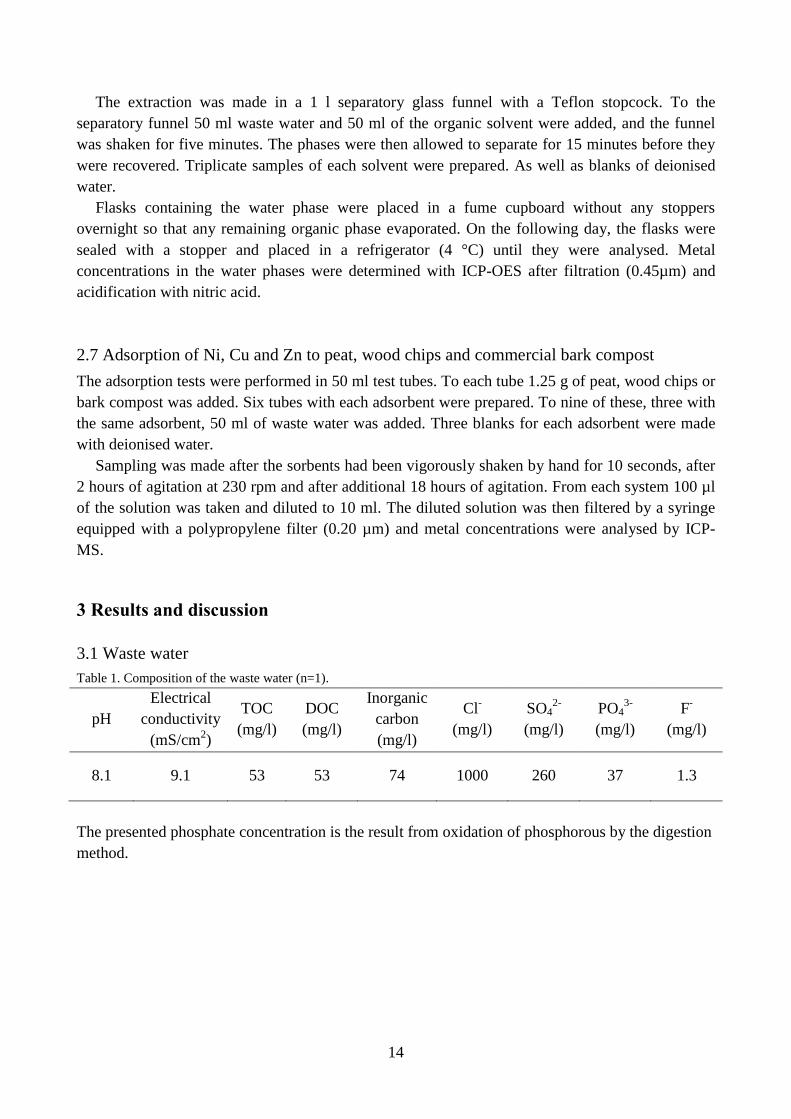
Table 1. Composition of the waste water (n=1).

pH

Electrical

conductivity

(mS/cm2)

TOC

(mg/l)

DOC

(mg/l)

Inorganic

carbon

(mg/l)

Cl-

(mg/l)

SO42-

(mg/l)

PO43-

(mg/l)

F-

(mg/l)

8.1 9.1 53 53 74 1000 260 37 1.3

The presented phosphate concentration is the result from oxidation of phosphorous by the digestion

method.

15

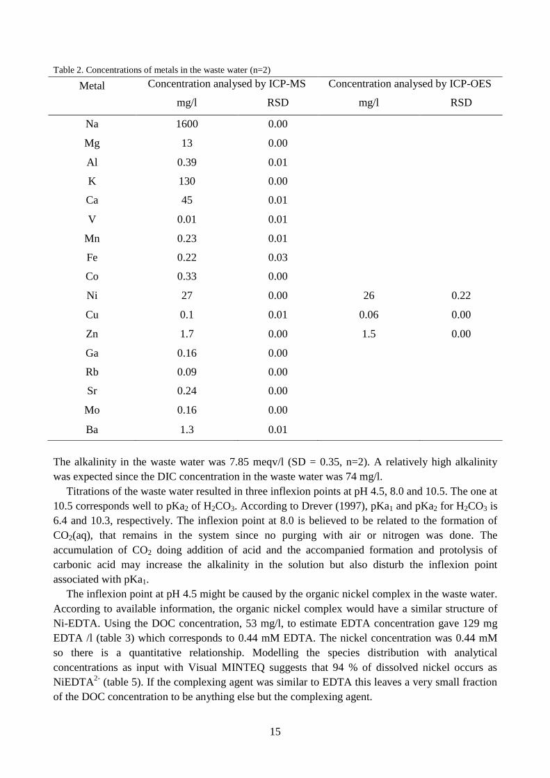
Table 2. Concentrations of metals in the waste water (n=2)

Metal Concentration analysed by ICP-MS Concentration analysed by ICP-OES

mg/l RSD mg/l RSD

Na 1600 0.00

Mg 13 0.00

Al 0.39 0.01

K 130 0.00

Ca 45 0.01

V 0.01 0.01

Mn 0.23 0.01

Fe 0.22 0.03

Co 0.33 0.00

Ni 27 0.00 26 0.22

Cu 0.1 0.01 0.06 0.00

Zn 1.7 0.00 1.5 0.00

Ga 0.16 0.00

Rb 0.09 0.00

Sr 0.24 0.00

Mo 0.16 0.00

Ba 1.3 0.01

The alkalinity in the waste water was 7.85 meqv/l (SD = 0.35, n=2). A relatively high alkalinity

was expected since the DIC concentration in the waste water was 74 mg/l.

Titrations of the waste water resulted in three inflexion points at pH 4.5, 8.0 and 10.5. The one at

10.5 corresponds well to pKa2 of H2CO3. According to Drever (1997), pKa1 and pKa2 for H2CO3 is

6.4 and 10.3, respectively. The inflexion point at 8.0 is believed to be related to the formation of

CO2(aq), that remains in the system since no purging with air or nitrogen was done. The

accumulation of CO2 doing addition of acid and the accompanied formation and protolysis of

carbonic acid may increase the alkalinity in the solution but also disturb the inflexion point

associated with pKa1.

The inflexion point at pH 4.5 might be caused by the organic nickel complex in the waste water.

According to available information, the organic nickel complex would have a similar structure of

Ni-EDTA. Using the DOC concentration, 53 mg/l, to estimate EDTA concentration gave 129 mg

EDTA /l (table 3) which corresponds to 0.44 mM EDTA. The nickel concentration was 0.44 mM

so there is a quantitative relationship. Modelling the species distribution with analytical

concentrations as input with Visual MINTEQ suggests that 94 % of dissolved nickel occurs as

NiEDTA2-

(table 5). If the complexing agent was similar to EDTA this leaves a very small fraction

of the DOC concentration to be anything else but the complexing agent.

16

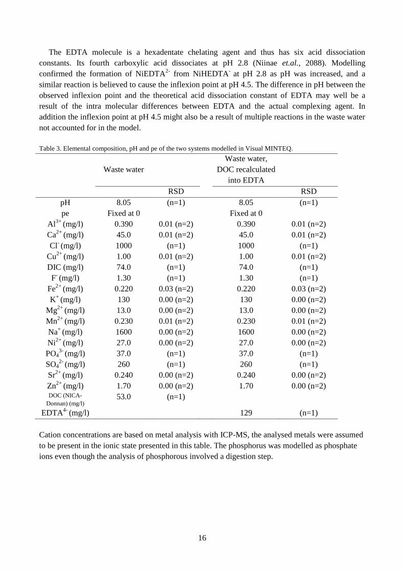
The EDTA molecule is a hexadentate chelating agent and thus has six acid dissociation

constants. Its fourth carboxylic acid dissociates at pH 2.8 (Niinae et.al., 2088). Modelling

confirmed the formation of NiEDTA2-

from NiHEDTA-

at pH 2.8 as pH was increased, and a

similar reaction is believed to cause the inflexion point at pH 4.5. The difference in pH between the

observed inflexion point and the theoretical acid dissociation constant of EDTA may well be a

result of the intra molecular differences between EDTA and the actual complexing agent. In

addition the inflexion point at pH 4.5 might also be a result of multiple reactions in the waste water

not accounted for in the model.

Table 3. Elemental composition, pH and pe of the two systems modelled in Visual MINTEQ.

Waste water

Waste water,

DOC recalculated

into EDTA

RSD RSD

pH 8.05 (n=1) 8.05 (n=1)

pe Fixed at 0 Fixed at 0

Al3+

(mg/l) 0.390 0.01 (n=2) 0.390 0.01 (n=2)

Ca2+

(mg/l)

45.0 0.01 (n=2) 45.0 0.01 (n=2)

Cl- (mg/l)

1000 (n=1) 1000 (n=1)

Cu2+

(mg/l)

1.00 0.01 (n=2) 1.00 0.01 (n=2)

DIC (mg/l) 74.0 (n=1) 74.0 (n=1)

F- (mg/l)

1.30 (n=1) 1.30 (n=1)

Fe2+

(mg/l)

0.220 0.03 (n=2) 0.220 0.03 (n=2)

K+

(mg/l)

130 0.00 (n=2) 130 0.00 (n=2)

Mg2+

(mg/l)

13.0 0.00 (n=2) 13.0 0.00 (n=2)

Mn2+

(mg/l)

0.230 0.01 (n=2) 0.230 0.01 (n=2)

Na+

(mg/l)

1600 0.00 (n=2) 1600 0.00 (n=2)

Ni2+

(mg/l)

27.0 0.00 (n=2) 27.0 0.00 (n=2)

PO43-

(mg/l)

37.0 (n=1) 37.0 (n=1)

SO42-

(mg/l)

260 (n=1) 260 (n=1)

Sr2+

(mg/l)

0.240 0.00 (n=2) 0.240 0.00 (n=2)

Zn2+

(mg/l)

1.70 0.00 (n=2) 1.70 0.00 (n=2) DOC (NICA-

Donnan) (mg/l) 53.0 (n=1)

EDTA4-

(mg/l)

129 (n=1)

Cation concentrations are based on metal analysis with ICP-MS, the analysed metals were assumed

to be present in the ionic state presented in this table. The phosphorus was modelled as phosphate

ions even though the analysis of phosphorous involved a digestion step.

17

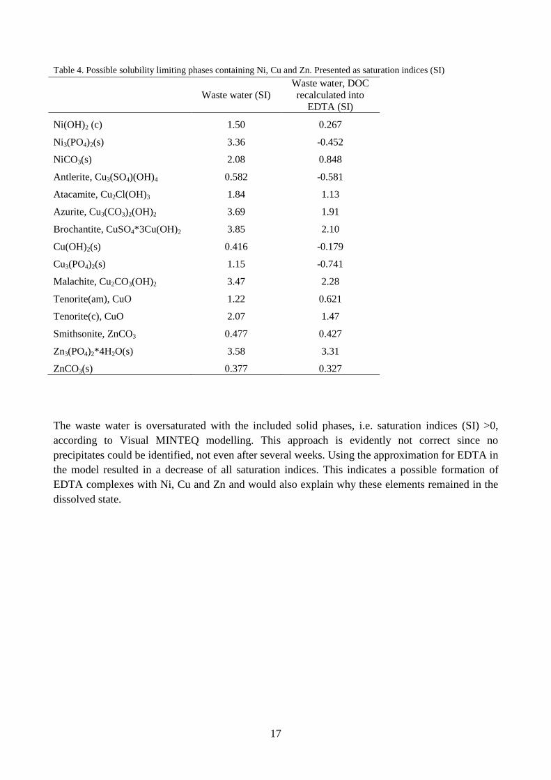
Table 4. Possible solubility limiting phases containing Ni, Cu and Zn. Presented as saturation indices (SI)

Waste water (SI)

Waste water, DOC

recalculated into

EDTA (SI)

Ni(OH)2 (c) 1.50 0.267

Ni3(PO4)2(s) 3.36 -0.452

NiCO3(s) 2.08 0.848

Antlerite, Cu3(SO4)(OH)4 0.582 -0.581

Atacamite, Cu2Cl(OH)3 1.84 1.13

Azurite, Cu3(CO3)2(OH)2 3.69 1.91

Brochantite, CuSO4*3Cu(OH)2 3.85 2.10

Cu(OH)2(s) 0.416 -0.179

Cu3(PO4)2(s) 1.15 -0.741

Malachite, Cu2CO3(OH)2 3.47 2.28

Tenorite(am), CuO 1.22 0.621

Tenorite(c), CuO 2.07 1.47

Smithsonite, ZnCO3 0.477 0.427

Zn3(PO4)2*4H2O(s) 3.58 3.31

ZnCO3(s) 0.377 0.327

The waste water is oversaturated with the included solid phases, i.e. saturation indices (SI) >0,

according to Visual MINTEQ modelling. This approach is evidently not correct since no

precipitates could be identified, not even after several weeks. Using the approximation for EDTA in

the model resulted in a decrease of all saturation indices. This indicates a possible formation of

EDTA complexes with Ni, Cu and Zn and would also explain why these elements remained in the

dissolved state.

18

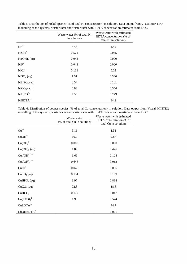
Table 5. Distribution of nickel species (% of total Ni concentration) in solution. Data output from Visual MINTEQ

modelling of the systems; waste water and waste water with EDTA concentration estimated from DOC

Waste water (% of total Ni

in solution)

Waste water with estimated

EDTA concentration (% of

total Ni in solution)

Ni2+

67.3 4.55

NiOH+

0.571 0.035

Ni(OH)2 (aq) 0.043 0.000

NiF+ 0.043 0.000

NiCl+ 0.111 0.02

NiSO4 (aq) 1.51 0.366

NiHPO4 (aq) 3.54 0.181

NiCO3 (aq) 6.03 0.354

NiHCO3+

4.56 0.279

NiEDTA2-

94.2

Table 6. Distribution of copper species (% of total Cu concentration) in solution. Data output from Visual MINTEQ

modelling of the systems; waste water and waste water with EDTA concentration estimated from DOC

Waste water

(% of total Cu in solution)

Waste water with estimated

EDTA concentration (% of

total Cu in solution)

Cu2+

5.11 1.51

CuOH+ 10.9 2.87

Cu(OH)3-

0.000 0.000

Cu(OH)2 (aq) 1.89 0.476

Cu2(OH)22+

1.66 0.124

Cu3(OH)42+

0.645 0.012

CuCl+ 0.045 0.036

CuSO4 (aq) 0.131 0.139

CuHPO4 (aq) 3.97 0.884

CuCO3 (aq) 72.5 18.6

CuHCO3+ 0.177 0.047

Cu(CO3)22-

1.90 0.574

CuEDTA2-

74.7

CuOHEDTA3-

0.021

19

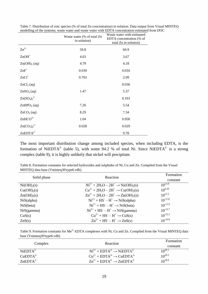
Table 7. Distribution of zinc species (% of total Zn concentration) in solution. Data output from Visual MINTEQ

modelling of the systems; waste water and waste water with EDTA concentration estimated from DOC

Waste water (% of total Zn

in solution)

Waste water with estimated

EDTA concentration (% of

total Zn in solution)

Zn2+

59.8 60.9

ZnOH+ 4.03 3.67

Zn(OH)2 (aq) 4.79 4.18

ZnF+ 0.039 0.034

ZnCl+ 0.763 2.09

ZnCl2 (aq) 0.036

ZnSO4 (aq) 1.47 5.37

Zn(SO4)22-

0.103

ZnHPO4 (aq) 7.20 5.54

ZnCO3 (aq) 8.29 7.34

ZnHCO3+

1.04 0.958

Zn(CO3)22-

0.028 0.029

ZnEDTA2-

9.78

The most important distribution change among included species, when including EDTA, is the

formation of NiEDTA2-

(table 5), with some 94.2 % of total Ni. Since NiEDTA2-

is a strong

complex (table 9), it is highly unlikely that nickel will precipitate.

Table 8. Formation constants for selected hydroxides and sulphides of Ni, Cu and Zn. Compiled from the Visual

MINTEQ data base (Vminteq30\type6.vdb)

Solid phase Reaction Formation

constant

Ni(OH)2(s) Ni2+

+ 2H2O – 2H+ → Ni(OH)2(s) 10

12.9

Cu(OH)2(s) Cu2+

+ 2H2O – 2H+ → Cu(OH)2(s) 10

9.29

Zn(OH)2(s) Zn2+

+ 2H2O – 2H+ → Zn(OH)2(s) 10

12.5

NiS(alpha) Ni2+

+ HS- – H

+ → NiS(alpha) 10

-5.52

NiS(beta) Ni2+

+ HS- – H

+ → NiS(beta) 10

-11.0

NiS(gamma) Ni2+

+ HS- – H

+ → NiS(gamma) 10

-12.7

CuS(s) Cu2+

+ HS- – H

+ → CuS(s) 10

-22.2

ZnS(s) Zn2+

+ HS- – H

+ → ZnS(s) 10

-10.8

Table 9. Formation constants for Me2+

EDTA complexes with Ni, Cu and Zn. Compiled from the Visual MINTEQ data

base (Vminteq30\type6.vdb)

Complex Reaction Formation

constant

NiEDTA2-

Ni2+

+ EDTA4-

→ NiEDTA2-

1020.1

CuEDTA2-

Cu2+

+ EDTA4-

→ CuEDTA2-

1020.5

ZnEDTA2-

Zn2+

+ EDTA4-

→ ZnEDTA2-

1018.0

20

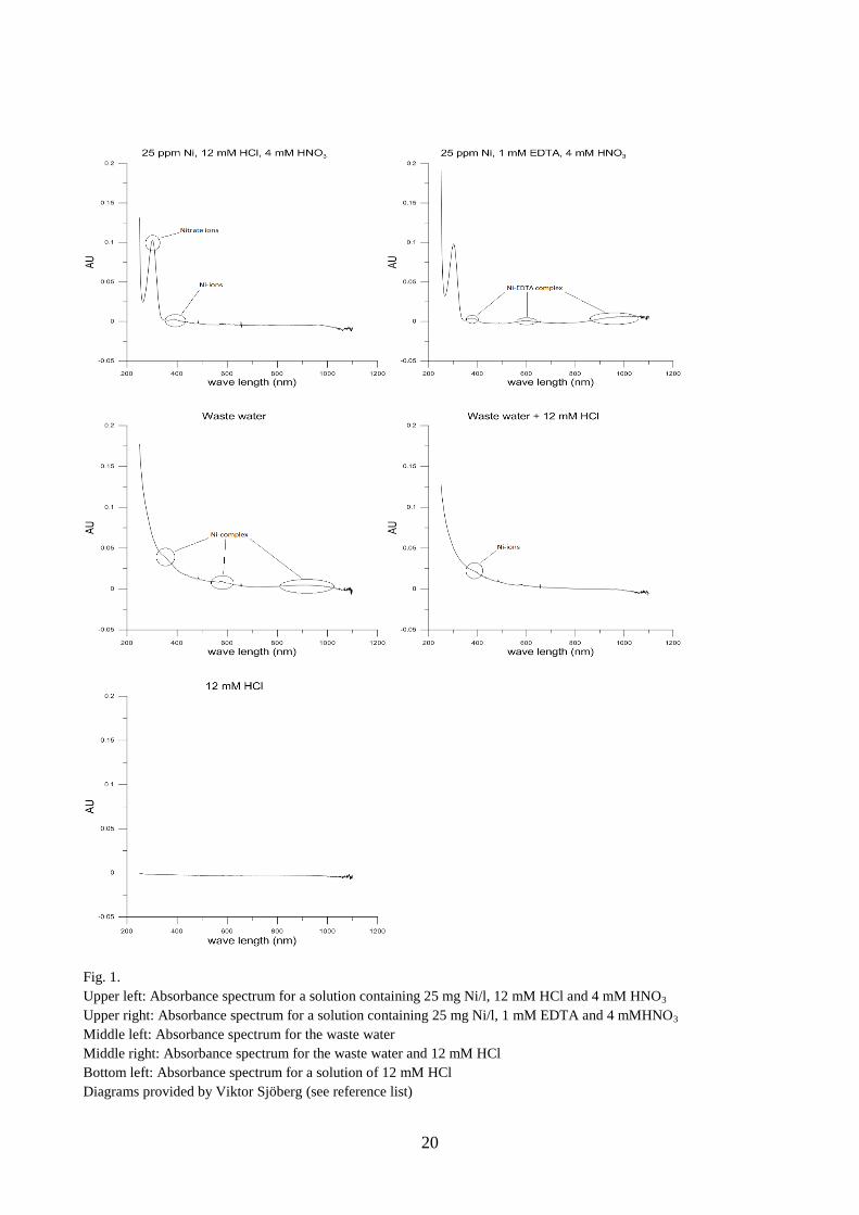
Fig. 1.

Upper left: Absorbance spectrum for a solution containing 25 mg Ni/l, 12 mM HCl and 4 mM HNO3

Upper right: Absorbance spectrum for a solution containing 25 mg Ni/l, 1 mM EDTA and 4 mMHNO3

Middle left: Absorbance spectrum for the waste water

Middle right: Absorbance spectrum for the waste water and 12 mM HCl

Bottom left: Absorbance spectrum for a solution of 12 mM HCl

Diagrams provided by Viktor Sjöberg (see reference list)

21

As shown in the upper right and middle left spectrum similar absorbance patterns was found for the

waste water and the prepared solution containing only Ni2+

and EDTA. Consequently the unknown

complexing agent in the waste water indeed has absorption properties that are similar to EDTA in

the selected wavelength region.

When the waste water was acidified to pH 2.6, middle right diagram (fig. 1), nickel dissociated

from the complexing agent because an absorbance pattern similar to that of upper left diagram (fig.

1) was produced. The dissociation process upon lowering of pH was modelled in Visual MINTEQ

(table 10) with EDTA as a proxy for the ligand and at two pH; 1.0 and 2.6. According to the Visual

MINTEQ modelling, pH 2.6 would not be low enough to dissociate Ni-EDTA to any large extent.

The results from the absorbance measurements (fig. 1) indicate that pH 2.6 was capable of

dissociating the organic nickel complex in the waste water. This indicates either a potential

difference between the complexing agent and EDTA, or an error in the modelling.

Table 10. Distribution of nickel species (% of total Ni concentration) in solution at pH 1.0 and 2.6. Data output from

Visual MINTEQ modelling of the waste water with an EDTA concentration estimated from DOC

Species distribution, pH 1.0 (%) Species distribution, pH 2.6 (%)

Ni2+

65.2 6.06

NiCl+

0.235 0.027

NiSO4 (aq) 0.745 0.440

NiEDTA2-

0.112 16.5

NiHEDTA- 17.3 75.1

NiH2EDTA (aq) 16.4 1.90

3.2 Size exclusion

Table 11. Concentrations of Ni, Cu and Zn after filtration of the waste water (n=2)

Average

pore

diameter

Non-filtered 1.0 µm 0.40 µm 0.20 µm 0.05 µm

Mean RSD Mean SD Mean SD Mean SD Mean SD

Ni (mg/l) 26 0.22 26 0.52 25 0.26 24 0.75 25 0.41

Cu (mg/l) 0.06 0.00 0.07 0.00 0.06 0.00 0.06 0.00 0.06 0.00

Zn (mg/l) 1.5 0.00 1.4 0.01 1.3 0.03 1.3 0.01 1.3 0.01

Filtration did not have any impact on the concentrations of Ni, Cu and Zn, in the water phase, why

these elements were dissolved or bound to carriers with diameters less than 0.05 µm can not be

excluded. Also these findings support that these elements remain in solution at high concentration

through association with a complexing agent.

22

3.3 The precipitation experiments

3.3.1 Impact of pH

Table 12. Composition of the aqueous phase, filtered (0.45µm) samples for Ni, Cu, Zn, DOC and DIC (n=3)

pH 4 pH 6 pH 8 pH 10 pH 12

Mean SD Mean SD Mean SD Mean SD Mean SD

pHinitial 4.0 0.01 6.0 0.02 8.1 0.03 10 0.01 12 0.01

pH24h 4.2 0.03 7.9 0.05 8.5 0.04 9.6 0.03 11 0.40

pH∆ +0.20 +1.9 +0.40 -0.40 -1.0

Ni(mg/l) 27 0.39 27 0.04 27 0.80 27 0.28 23 0.51

Cu(mg/l) 0.06 0.00 0.06 0.00 0.06 0.00 0.06 0.00 0.06 0.00

Zn(mg/l) 1.6 0.07 1.6 0.08 1.6 0.04 0.99 0.22 0.11 0.00

DOC(mg/l) 51 1.2 55 1.4 65 17 55 1.7 52 2.1

DIC(mg/l) 0.00 0.00 10 1.2 70 0.00 82 6.8 106 3.6

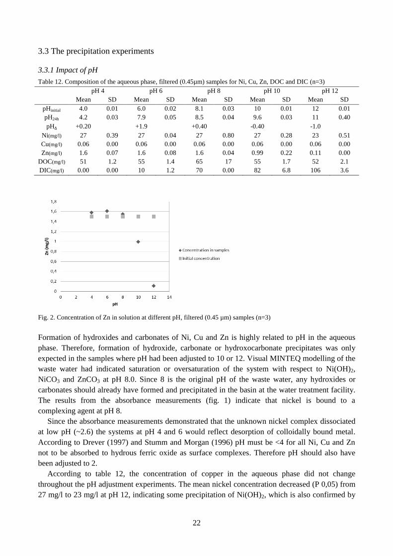
Fig. 2. Concentration of Zn in solution at different pH, filtered (0.45 µm) samples (n=3)

Formation of hydroxides and carbonates of Ni, Cu and Zn is highly related to pH in the aqueous

phase. Therefore, formation of hydroxide, carbonate or hydroxocarbonate precipitates was only

expected in the samples where pH had been adjusted to 10 or 12. Visual MINTEQ modelling of the

waste water had indicated saturation or oversaturation of the system with respect to Ni(OH)2,

NiCO3 and ZnCO3 at pH 8.0. Since 8 is the original pH of the waste water, any hydroxides or

carbonates should already have formed and precipitated in the basin at the water treatment facility.

The results from the absorbance measurements (fig. 1) indicate that nickel is bound to a

complexing agent at pH 8.

Since the absorbance measurements demonstrated that the unknown nickel complex dissociated

at low pH (~2.6) the systems at pH 4 and 6 would reflect desorption of colloidally bound metal.

According to Drever (1997) and Stumm and Morgan (1996) pH must be <4 for all Ni, Cu and Zn

not to be absorbed to hydrous ferric oxide as surface complexes. Therefore pH should also have

been adjusted to 2.

According to table 12, the concentration of copper in the aqueous phase did not change

throughout the pH adjustment experiments. The mean nickel concentration decreased (P 0,05) from

27 mg/l to 23 mg/l at pH 12, indicating some precipitation of Ni(OH)2, which is also confirmed by

23

Visual MINTEQ modelling. Evidently a high pH was not enough to completely separate nickel

from the complexing agent present in the water. This is also indicated by Visual MINTEQ

modelling of the EDTA system at pH 12.0 (table 13), when 90 % of dissolved nickel still is present

as an EDTA complex.

The organic carbon concentrations were independent of pH. The concentration in the samples

adjusted to pH 8 is probably a result of contamination due to its relatively large SD value.

Concentrations of inorganic carbon are closely related to pH and this relationship will be discussed

in more detail under heading 3.3.3.

At pH 8, which was the waste waters original pH, approximately 61 % of total zinc in solution

occurs as Zn2+

ions, according to output of Visual MINTEQ modelling of waste water with EDTA

present (table 7). These zinc ions are free to form hydroxides as pH increases, which could be the

reason for observed decrease of zinc concentrations in solutions at higher pH (fig. 2).

According to the Visual MINTEQ modelling of the waste water with EDTA as proxy for the

ligand at pH 10, the saturation indices for Ni(OH)2(c), Cu(OH)2 and Zn(OH)2(beta) were 3.035,

1.793 and 0.534 respectively. At pH 12 saturation indices for Ni, Cu and Zn hydroxides decrease

due to the formation of negatively charged hydroxide complexes in solution. The majority of Ni

and Cu are estimated to remain in solution as EDTA complexes even as pH increases.

Table 13. Distribution of nickel species (% of total Ni concentration) in solution at pH 12.0. Data output from Visual

MINTEQ modelling of the waste water with an EDTA concentration estimated from DOC

Species distribution (%)

Ni(OH)2 (aq) 0.733

Ni(OH)3-

9.29

NiEDTA2-

49.0

NiOHEDTA3-

41.0

3.3.2 Precipitation of sulphides

Table 14. Composition of the aqueous phase, filtered (0.45µm) samples for Ni, Cu, Zn, DOC and DIC (n=3)

pH 4 pH 6 pH 8 pH 10 pH 12

Mean SD Mean SD Mean SD Mean SD Mean SD

pHinitial 3.9 0.09 6.0 0.01 8.0 0.02 10 0.01 12 0.01

pH24h 4.3 0.21 7.8 0.02 8.6 0.03 9.5 0.07 11 0.08

pH∆ +0.40 +1.8 +0.60 -0.50 -1.0

Ni(mg/l) 22 0.74 25 0.41 25 0.30 25 0.47 23 0.94

Cu(mg/l) 0.00 0.00 0.00 0.00 0.00 0.00 0.00 0.00 0.00 0.00

Zn(mg/l) 0.91 0.04 0.59 0.09 0.26 0.02 0.35 0.03 0.12 0.00

DOC(mg/l) 53 0.47 54 0.82 55 0.94 54 0.47 54 1.7

DIC(mg/l) 0.00 0.00 9.1 0.74 76 0.82 80 3.8 120 1.4

24

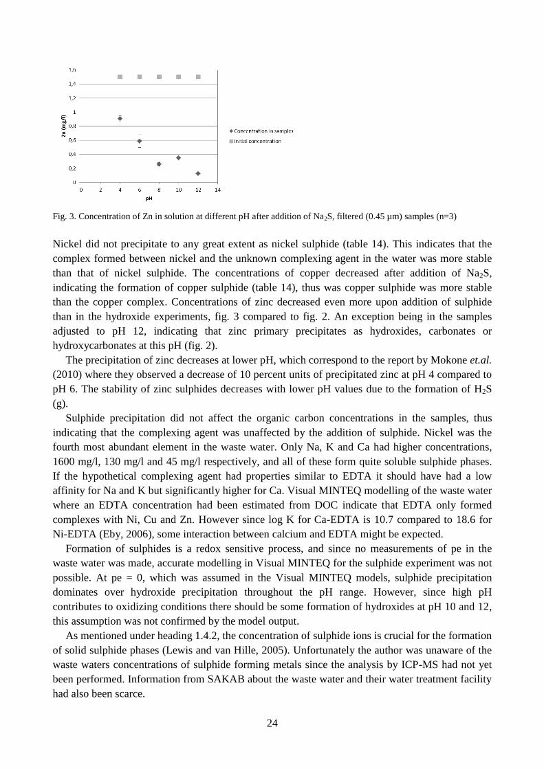
Fig. 3. Concentration of Zn in solution at different pH after addition of Na2S, filtered (0.45 µm) samples (n=3)

Nickel did not precipitate to any great extent as nickel sulphide (table 14). This indicates that the

complex formed between nickel and the unknown complexing agent in the water was more stable

than that of nickel sulphide. The concentrations of copper decreased after addition of Na2S,

indicating the formation of copper sulphide (table 14), thus was copper sulphide was more stable

than the copper complex. Concentrations of zinc decreased even more upon addition of sulphide

than in the hydroxide experiments, fig. 3 compared to fig. 2. An exception being in the samples

adjusted to pH 12, indicating that zinc primary precipitates as hydroxides, carbonates or

hydroxycarbonates at this pH (fig. 2).

The precipitation of zinc decreases at lower pH, which correspond to the report by Mokone et.al.

(2010) where they observed a decrease of 10 percent units of precipitated zinc at pH 4 compared to

pH 6. The stability of zinc sulphides decreases with lower pH values due to the formation of H2S

(g).

Sulphide precipitation did not affect the organic carbon concentrations in the samples, thus

indicating that the complexing agent was unaffected by the addition of sulphide. Nickel was the

fourth most abundant element in the waste water. Only Na, K and Ca had higher concentrations,

1600 mg/l, 130 mg/l and 45 mg/l respectively, and all of these form quite soluble sulphide phases.

If the hypothetical complexing agent had properties similar to EDTA it should have had a low

affinity for Na and K but significantly higher for Ca. Visual MINTEQ modelling of the waste water

where an EDTA concentration had been estimated from DOC indicate that EDTA only formed

complexes with Ni, Cu and Zn. However since log K for Ca-EDTA is 10.7 compared to 18.6 for

Ni-EDTA (Eby, 2006), some interaction between calcium and EDTA might be expected.

Formation of sulphides is a redox sensitive process, and since no measurements of pe in the

waste water was made, accurate modelling in Visual MINTEQ for the sulphide experiment was not

possible. At pe = 0, which was assumed in the Visual MINTEQ models, sulphide precipitation

dominates over hydroxide precipitation throughout the pH range. However, since high pH

contributes to oxidizing conditions there should be some formation of hydroxides at pH 10 and 12,

this assumption was not confirmed by the model output.

As mentioned under heading 1.4.2, the concentration of sulphide ions is crucial for the formation

of solid sulphide phases (Lewis and van Hille, 2005). Unfortunately the author was unaware of the

waste waters concentrations of sulphide forming metals since the analysis by ICP-MS had not yet

been performed. Information from SAKAB about the waste water and their water treatment facility

had also been scarce.

25

An estimation of the required amount of Na2S was made from a nickel sulphide molar ratio of

approximately 1:10, resulting in that 30 mg Na2S was added to 100 ml waste water. This might be a

contributing factor to why precipitation of nickel sulphide was unsuccessful.

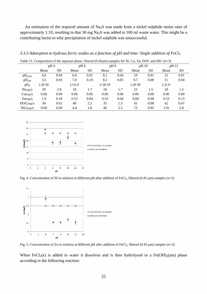
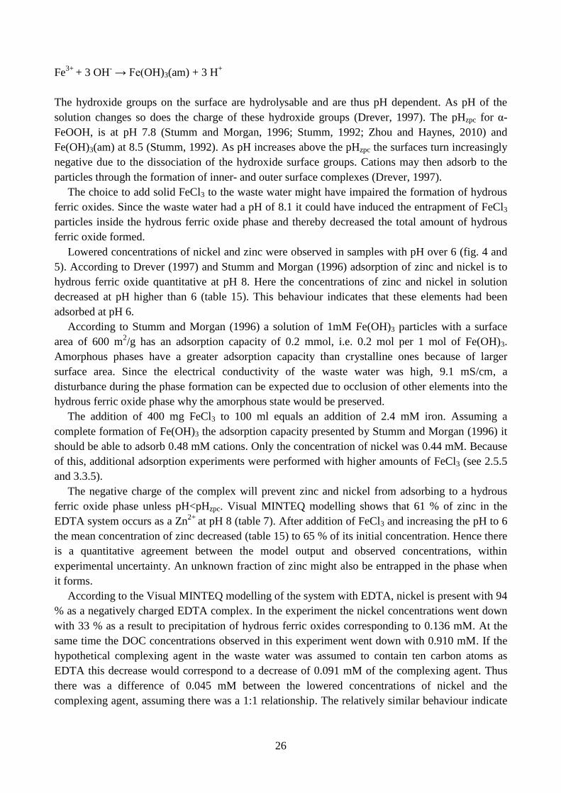
3.3.3 Adsorption to hydrous ferric oxides as a function of pH and time: Single addition of FeCl3

Table 15. Composition of the aqueous phase, filtered (0.45µm) samples for Ni, Cu, Zn, DOC and DIC (n=3)

pH 4 pH 6 pH 8 pH 10 pH 12

Mean SD Mean SD Mean SD Mean SD Mean SD

pHinitial 4.0 0.04 6.0 0.01 8.1 0.04 10 0.01 12 0.01

pH24h 3.5 0.03 7.0 0.19 8.2 0.05 9.7 0.00 11 0.04

pH∆ (-)0.50 (+)1.0 (+)0.10 (-)0.30 (-)1.0

Ni(mg/l) 29 2.8 18 1.7 18 1.7 23 1.5 18 1.5

Cu(mg/l) 0.06 0.00 0.06 0.00 0.06 0.00 0.06 0.00 0.06 0.00

Zn(mg/l) 1.9 0.18 0.53 0.04 0.53 0.04 0.69 0.08 0.53 0.13

DOC(mg/l) 39 0.01 40 2.2 35 1.3 41 0.98 42 0.47

DIC(mg/l) 0.00 0.00 4.4 1.8 40 2.5 72 0.95 119 2.8

Fig. 4. Concentration of Ni in solution at different pH after addition of FeCl3, filtered (0.45 µm) samples (n=3)

Fig. 5. Concentration of Zn in solution at different pH after addition of FeCl3, filtered (0.45 µm) samples (n=3)

When FeCl3(s) is added to water it dissolves and is then hydrolysed to a Fe(OH)3(am) phase

according to the following reaction:

26

Fe3+

+ 3 OH- → Fe(OH)3(am) + 3 H

+

The hydroxide groups on the surface are hydrolysable and are thus pH dependent. As pH of the

solution changes so does the charge of these hydroxide groups (Drever, 1997). The pHzpc for α-

FeOOH, is at pH 7.8 (Stumm and Morgan, 1996; Stumm, 1992; Zhou and Haynes, 2010) and

Fe(OH)3(am) at 8.5 (Stumm, 1992). As pH increases above the pHzpc the surfaces turn increasingly

negative due to the dissociation of the hydroxide surface groups. Cations may then adsorb to the

particles through the formation of inner- and outer surface complexes (Drever, 1997).

The choice to add solid FeCl3 to the waste water might have impaired the formation of hydrous

ferric oxides. Since the waste water had a pH of 8.1 it could have induced the entrapment of FeCl3

particles inside the hydrous ferric oxide phase and thereby decreased the total amount of hydrous

ferric oxide formed.

Lowered concentrations of nickel and zinc were observed in samples with pH over 6 (fig. 4 and

5). According to Drever (1997) and Stumm and Morgan (1996) adsorption of zinc and nickel is to

hydrous ferric oxide quantitative at pH 8. Here the concentrations of zinc and nickel in solution

decreased at pH higher than 6 (table 15). This behaviour indicates that these elements had been

adsorbed at pH 6.

According to Stumm and Morgan (1996) a solution of 1mM Fe(OH)3 particles with a surface

area of 600 m2/g has an adsorption capacity of 0.2 mmol, i.e. 0.2 mol per 1 mol of Fe(OH)3.

Amorphous phases have a greater adsorption capacity than crystalline ones because of larger

surface area. Since the electrical conductivity of the waste water was high, 9.1 mS/cm, a

disturbance during the phase formation can be expected due to occlusion of other elements into the

hydrous ferric oxide phase why the amorphous state would be preserved.

The addition of 400 mg FeCl3 to 100 ml equals an addition of 2.4 mM iron. Assuming a

complete formation of Fe(OH)3 the adsorption capacity presented by Stumm and Morgan (1996) it

should be able to adsorb 0.48 mM cations. Only the concentration of nickel was 0.44 mM. Because

of this, additional adsorption experiments were performed with higher amounts of FeCl3 (see 2.5.5

and 3.3.5).

The negative charge of the complex will prevent zinc and nickel from adsorbing to a hydrous

ferric oxide phase unless pH<pHzpc. Visual MINTEQ modelling shows that 61 % of zinc in the

EDTA system occurs as a Zn2+

at pH 8 (table 7). After addition of FeCl3 and increasing the pH to 6

the mean concentration of zinc decreased (table 15) to 65 % of its initial concentration. Hence there

is a quantitative agreement between the model output and observed concentrations, within

experimental uncertainty. An unknown fraction of zinc might also be entrapped in the phase when

it forms.

According to the Visual MINTEQ modelling of the system with EDTA, nickel is present with 94

% as a negatively charged EDTA complex. In the experiment the nickel concentrations went down

with 33 % as a result to precipitation of hydrous ferric oxides corresponding to 0.136 mM. At the

same time the DOC concentrations observed in this experiment went down with 0.910 mM. If the

hypothetical complexing agent in the waste water was assumed to contain ten carbon atoms as

EDTA this decrease would correspond to a decrease of 0.091 mM of the complexing agent. Thus

there was a difference of 0.045 mM between the lowered concentrations of nickel and the

complexing agent, assuming there was a 1:1 relationship. The relatively similar behaviour indicate

27

that the nickel complex was physically entrapped in the settling hydrous ferric oxide and the same

would apply to zinc.

The copper concentrations remain constant in these experiments which would be the case if the

dominating species lacked affinity towards the hydrous ferric oxide phase. According to the Visual

MINTEQ modelling of the EDTA system approximately 5 % of the copper species were cationic

(table 6). These two approaches support each other why the general conclusion would be adsorption

is minimal.

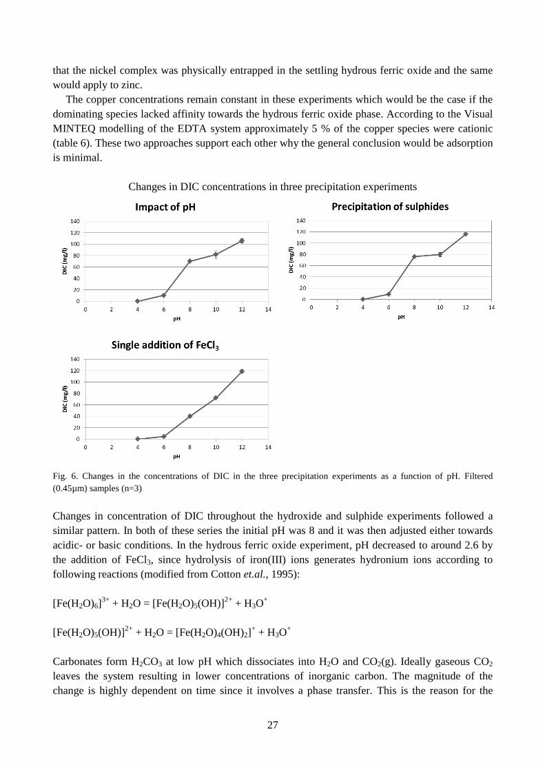
Changes in DIC concentrations in three precipitation experiments

Fig. 6. Changes in the concentrations of DIC in the three precipitation experiments as a function of pH. Filtered

(0.45µm) samples (n=3)

Changes in concentration of DIC throughout the hydroxide and sulphide experiments followed a

similar pattern. In both of these series the initial pH was 8 and it was then adjusted either towards

acidic- or basic conditions. In the hydrous ferric oxide experiment, pH decreased to around 2.6 by

the addition of FeCl3, since hydrolysis of iron(III) ions generates hydronium ions according to

following reactions (modified from Cotton et.al., 1995):

[Fe(H2O)6]3+

+ H2O = [Fe(H2O)5(OH)]2+

+ H3O+

[Fe(H2O)5(OH)]2+

+ H2O = [Fe(H2O)4(OH)2]+ + H3O

+

Carbonates form H2CO3 at low pH which dissociates into H2O and CO2(g). Ideally gaseous CO2

leaves the system resulting in lower concentrations of inorganic carbon. The magnitude of the

change is highly dependent on time since it involves a phase transfer. This is the reason for the

28

lower concentration of inorganic carbon found at pH 8 after addition of FeCl3 compared to the

other two precipitation experiments (fig. 6).

The inproportional increase of inorganic carbon at high pH is believed to be caused by the

addition of NaOH. Both NaOH pellets and NaOH solutions accumulate carbonates from their

contact with atmospheric CO2(g).

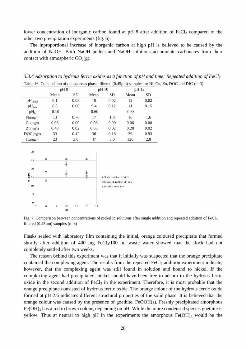
3.3.4 Adsorption to hydrous ferric oxides as a function of pH and time: Repeated addition of FeCl3

Table 16. Composition of the aqueous phase, filtered (0.45µm) samples for Ni, Cu, Zn, DOC and DIC (n=3)

pH 8 pH 10 pH 12

Mean SD Mean SD Mean SD

pHinitial 8.1 0.03 10 0.02 12 0.02

pH24h 8.0 0.06 9.4 0.12 11 0.15

pH∆ -0.10 -0.60 -0.63

Ni(mg/l) 13 0.76 17 1.8 16 1.6

Cu(mg/l) 0.06 0.00 0.06 0.00 0.06 0.00

Zn(mg/l) 0.48 0.02 0.65 0.02 0.28 0.02

DOC(mg/l) 33 0.42 36 0.18 39 0.93

IC(mg/l) 23 3.0 47 3.0 120 2.8

Fig. 7. Comparison between concentrations of nickel in solutions after single addition and repeated addition of FeCl3,

filtered (0.45µm) samples (n=3)

Flasks sealed with laboratory film containing the initial, orange coloured precipitate that formed

shortly after addition of 400 mg FeCl3/100 ml waste water showed that the flock had not

completely settled after two weeks.

The reason behind this experiment was that it initially was suspected that the orange precipitate

contained the complexing agent. The results from the repeated FeCl3 addition experiment indicate,

however, that the complexing agent was still found in solution and bound to nickel. If the

complexing agent had precipitated, nickel should have been free to adsorb to the hydrous ferric

oxide in the second addition of FeCl3 in the experiment. Therefore, it is most probable that the

orange precipitate consisted of hydrous ferric oxide. The orange colour of the hydrous ferric oxide

formed at pH 2.6 indicates different structural properties of the solid phase. It is believed that the

orange colour was caused by the presence of goethite, FeOOH(s). Freshly precipitated amorphous

Fe(OH)3 has a red to brown colour, depending on pH. While the more condensed species goethite is

yellow. Thus at neutral to high pH in the experiments the amorphous Fe(OH)3 would be the

29

candidate. At low pH the yellow colour indicate a higher abundance of goethite, possibly as a

response to lower precipitation rate.

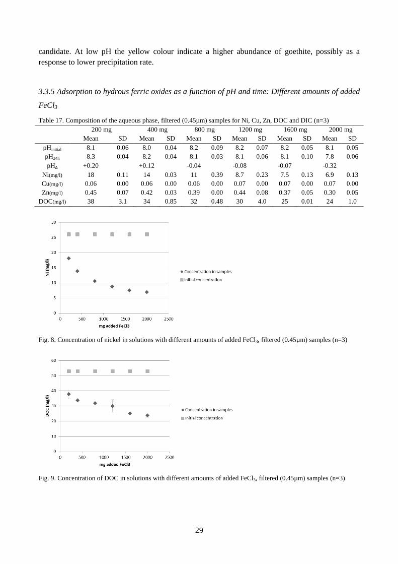
3.3.5 Adsorption to hydrous ferric oxides as a function of pH and time: Different amounts of added

FeCl3

Table 17. Composition of the aqueous phase, filtered (0.45µm) samples for Ni, Cu, Zn, DOC and DIC (n=3)

200 mg 400 mg 800 mg 1200 mg 1600 mg 2000 mg

Mean SD Mean SD Mean SD Mean SD Mean SD Mean SD

pHinitial 8.1 0.06 8.0 0.04 8.2 0.09 8.2 0.07 8.2 0.05 8.1 0.05

pH24h 8.3 0.04 8.2 0.04 8.1 0.03 8.1 0.06 8.1 0.10 7.8 0.06

pH∆ +0.20 +0.12 -0.04 -0.08 -0.07 -0.32

Ni(mg/l) 18 0.11 14 0.03 11 0.39 8.7 0.23 7.5 0.13 6.9 0.13

Cu(mg/l) 0.06 0.00 0.06 0.00 0.06 0.00 0.07 0.00 0.07 0.00 0.07 0.00

Zn(mg/l) 0.45 0.07 0.42 0.03 0.39 0.00 0.44 0.08 0.37 0.05 0.30 0.05

DOC(mg/l) 38 3.1 34 0.85 32 0.48 30 4.0 25 0.01 24 1.0

Fig. 8. Concentration of nickel in solutions with different amounts of added FeCl3, filtered (0.45µm) samples (n=3)

Fig. 9. Concentration of DOC in solutions with different amounts of added FeCl3, filtered (0.45µm) samples (n=3)

30

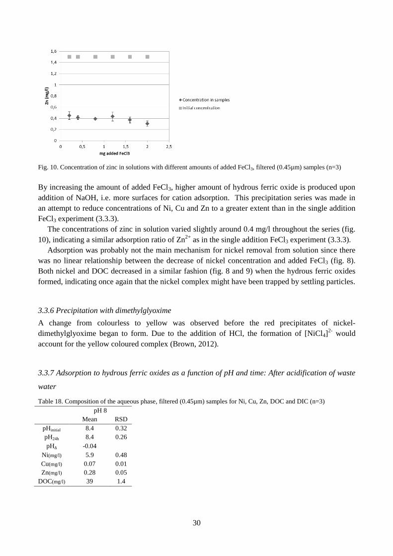
Fig. 10. Concentration of zinc in solutions with different amounts of added FeCl3, filtered (0.45µm) samples (n=3)

By increasing the amount of added FeCl3, higher amount of hydrous ferric oxide is produced upon

addition of NaOH, i.e. more surfaces for cation adsorption. This precipitation series was made in

an attempt to reduce concentrations of Ni, Cu and Zn to a greater extent than in the single addition

FeCl3 experiment (3.3.3).

The concentrations of zinc in solution varied slightly around 0.4 mg/l throughout the series (fig.

10), indicating a similar adsorption ratio of Zn2+

as in the single addition FeCl3 experiment (3.3.3).

Adsorption was probably not the main mechanism for nickel removal from solution since there

was no linear relationship between the decrease of nickel concentration and added FeCl3 (fig. 8).

Both nickel and DOC decreased in a similar fashion (fig. 8 and 9) when the hydrous ferric oxides

formed, indicating once again that the nickel complex might have been trapped by settling particles.

3.3.6 Precipitation with dimethylglyoxime

A change from colourless to yellow was observed before the red precipitates of nickel-

dimethylglyoxime began to form. Due to the addition of HCl, the formation of [NiCl4]2-

would

account for the yellow coloured complex (Brown, 2012).

3.3.7 Adsorption to hydrous ferric oxides as a function of pH and time: After acidification of waste

water

Table 18. Composition of the aqueous phase, filtered (0.45µm) samples for Ni, Cu, Zn, DOC and DIC (n=3)

pH 8

Mean RSD

pHinitial 8.4 0.32

pH24h 8.4 0.26

pH∆ -0.04

Ni(mg/l) 5.9 0.48

Cu(mg/l) 0.07 0.01

Zn(mg/l) 0.28 0.05

DOC(mg/l) 39 1.4

31

The concentration of nickel in the solution phase decreased from 26 mg/l to 5.9 mg/l. In the

previous precipitation experiment where 2000 mg FeCl3 was added to 100 ml of waste water

(3.3.5), the nickel concentration decreased to 6.9 mg/l (table 17). Acidification of waste water

seems not to have improved the ratio of nickel adsorption to hydrous ferric oxide.

To model the iron impact, the concentration 6900 mg/l Fe3+

was used as input, as well as EDTA

estimated from DOC and modelled pH at; 0.5, 1.0, 2.0, 3.0, 4.0, 5.0, 6.0, 7.0 and 8.0. The

concentration 6900 mg/l Fe3+

corresponds to the concentration of Fe used in this precipitation

experiment. The output indicates that the Fe-EDTA complex dominates at pH <6.0. At pH 6.0 iron

oxide, oxyhydroxide and hydroxide phases are saturated. As pH increases above 6.0 the fraction of

nickel EDTA complexes increase. At pH 8.0, as was the pH to which the samples were adjusted to,

66 % of dissolved nickel species should be Ni2+

according to Visual MINTEQ output. The same

output indicates that 78 % of EDTA occurs as different Fe-EDTA complexes.

The addition of Fe3+

to a concentration of 6900 mg/l lowered the pH of the waste water to

slightly below 1.0, where EDTA is exclusively coordinated to iron.

So it seems acidification of waste water was unnecessary for the dissociation of Ni-EDTA

complexes. The high concentrations of Fe3+

probably induced the formation of Fe-EDTA

complexes. If this modelling output is completely applicable for the complexing agent in the waste

water is unsure.

3.3.8 Adsorption to hydrous ferric oxides as a function of pH and time: After acid oxidative

digestion of waste water

Table 19. Initial concentrations and concentrations of Ni, Cu and Zn in digested waste water before precipitations. Non-

digested sample (n=2). Digested samples (n=3)

Ni (mg/l) Cu (mg/l) Zn (mg/l)

Mean SD Mean SD Mean SD

Non-digested sample 27 0.00 0.10 0.01 1.7 0.00

Digested samples 28 0.30 0.07 0.00 1.4 0.01

Due to the addition of FeCl3 and NaOH to samples during the precipitation experiment, high

concentrations of iron, chloride and sodium ions caused matrix problems during analysis by ICP-

MS. The most crucial interference species during the analysis of 60

Ni were 23

Na and 37

Cl forming

NaCl, and 25

Mg and 35

Cl forming MgCl+. The nickel concentration of 24 µg/l with an SD of 3.4

was determined by the use of interference correlation equations. These equations are very

dependent on the plasmas effect and where in the plasma the sampling occurs (Viktor Sjöberg,

pers-comm).

32

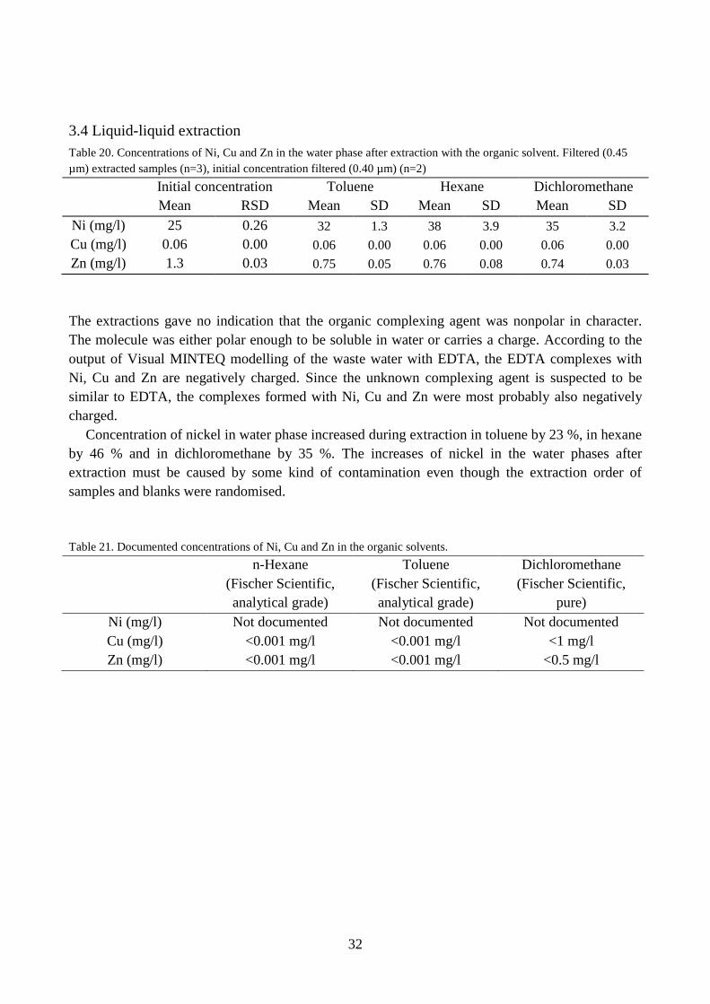
3.4 Liquid-liquid extraction

Table 20. Concentrations of Ni, Cu and Zn in the water phase after extraction with the organic solvent. Filtered (0.45

µm) extracted samples (n=3), initial concentration filtered (0.40 µm) (n=2)

Initial concentration Toluene Hexane Dichloromethane

Mean RSD Mean SD Mean SD Mean SD

Ni (mg/l) 25 0.26 32 1.3 38 3.9 35 3.2

Cu (mg/l) 0.06 0.00 0.06 0.00 0.06 0.00 0.06 0.00

Zn (mg/l) 1.3 0.03 0.75 0.05 0.76 0.08 0.74 0.03

The extractions gave no indication that the organic complexing agent was nonpolar in character.

The molecule was either polar enough to be soluble in water or carries a charge. According to the

output of Visual MINTEQ modelling of the waste water with EDTA, the EDTA complexes with

Ni, Cu and Zn are negatively charged. Since the unknown complexing agent is suspected to be

similar to EDTA, the complexes formed with Ni, Cu and Zn were most probably also negatively

charged.

Concentration of nickel in water phase increased during extraction in toluene by 23 %, in hexane

by 46 % and in dichloromethane by 35 %. The increases of nickel in the water phases after

extraction must be caused by some kind of contamination even though the extraction order of

samples and blanks were randomised.

Table 21. Documented concentrations of Ni, Cu and Zn in the organic solvents.

n-Hexane

(Fischer Scientific,

analytical grade)

Toluene

(Fischer Scientific,

analytical grade)

Dichloromethane

(Fischer Scientific,

pure)

Ni (mg/l) Not documented Not documented Not documented

Cu (mg/l) <0.001 mg/l <0.001 mg/l <1 mg/l

Zn (mg/l) <0.001 mg/l <0.001 mg/l <0.5 mg/l

33

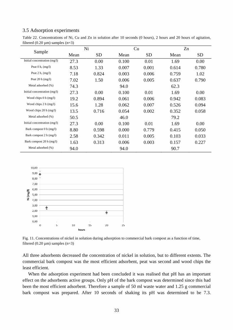
3.5 Adsorption experiments

Table 22. Concentrations of Ni, Cu and Zn in solution after 10 seconds (0 hours), 2 hours and 20 hours of agitation,

filtered (0.20 µm) samples (n=3)

Sample Ni Cu Zn

Mean SD Mean SD Mean SD Initial concentration (mg/l) 27.3 0.00 0.100 0.01 1.69 0.00

Peat 0 h, (mg/l) 8.53 1.33 0.007 0.001 0.614 0.780 Peat 2 h, (mg/l) 7.18 0.824 0.003 0.006 0.759 1.02 Peat 20 h (mg/l) 7.02 1.50 0.006 0.005 0.637 0.790

Metal adsorbed (%) 74.3 94.0 62.3 Initial concentration (mg/l) 27.3 0.00 0.100 0.01 1.69 0.00

Wood chips 0 h (mg/l) 19.2 0.894 0.061 0.006 0.942 0.083 Wood chips 2 h (mg/l) 15.6 1.28 0.062 0.007 0.526 0.094

Wood chips 20 h (mg/l) 13.5 0.716 0.054 0.002 0.352 0.058 Metal adsorbed (%) 50.5 46.0 79.2

Initial concentration (mg/l) 27.3 0.00 0.100 0.01 1.69 0.00 Bark compost 0 h (mg/l) 8.80 0.598 0.000 0.779 0.415 0.050 Bark compost 2 h (mg/l) 2.58 0.342 0.011 0.005 0.103 0.033

Bark compost 20 h (mg/l) 1.63 0.313 0.006 0.003 0.157 0.227 Metal adsorbed (%) 94.0 94.0 90.7

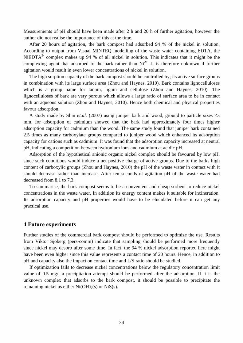
Fig. 11. Concentrations of nickel in solution during adsorption to commercial bark compost as a function of time,

filtered (0.20 µm) samples (n=3)

All three adsorbents decreased the concentration of nickel in solution, but to different extents. The

commercial bark compost was the most efficient adsorbent, peat was second and wood chips the

least efficient.

When the adsorption experiment had been concluded it was realised that pH has an important

effect on the adsorbents active groups. Only pH of the bark compost was determined since this had

been the most efficient adsorbent. Therefore a sample of 50 ml waste water and 1.25 g commercial

bark compost was prepared. After 10 seconds of shaking its pH was determined to be 7.3.

34

Measurements of pH should have been made after 2 h and 20 h of further agitation, however the

author did not realise the importance of this at the time.

After 20 hours of agitation, the bark compost had adsorbed 94 % of the nickel in solution.

According to output from Visual MINTEQ modelling of the waste water containing EDTA, the

NiEDTA2-

complex makes up 94 % of all nickel in solution. This indicates that it might be the

complexing agent that adsorbed to the bark rather than Ni2+

. It is therefore unknown if further

agitation would result in even lower concentrations of nickel in solution.

The high sorption capacity of the bark compost should be controlled by; its active surface groups

in combination with its large surface area (Zhou and Haynes, 2010). Bark contains lignocelluloses

which is a group name for tannin, lignin and cellulose (Zhou and Haynes, 2010). The

lignocelluloses of bark are very porous which allows a large ratio of surface area to be in contact

with an aqueous solution (Zhou and Haynes, 2010). Hence both chemical and physical properties

favour adsorption.

A study made by Shin et.al. (2007) using juniper bark and wood, ground to particle sizes <3

mm, for adsorption of cadmium showed that the bark had approximately four times higher

adsorption capacity for cadmium than the wood. The same study found that juniper bark contained

2.5 times as many carboxylate groups compared to juniper wood which enhanced its adsorption

capacity for cations such as cadmium. It was found that the adsorption capacity increased at neutral

pH, indicating a competition between hydronium ions and cadmium at acidic pH.

Adsorption of the hypothetical anionic organic nickel complex should be favoured by low pH,

since such conditions would induce a net positive charge of active groups. Due to the barks high

content of carboxylic groups (Zhou and Haynes, 2010) the pH of the waste water in contact with it

should decrease rather than increase. After ten seconds of agitation pH of the waste water had

decreased from 8.1 to 7.3.

To summarise, the bark compost seems to be a convenient and cheap sorbent to reduce nickel

concentrations in the waste water. In addition its energy content makes it suitable for incineration.

Its adsorption capacity and pH properties would have to be elucidated before it can get any

practical use.

4 Future experiments

Further studies of the commercial bark compost should be performed to optimize the use. Results

from Viktor Sjöberg (pers-comm) indicate that sampling should be performed more frequently

since nickel may desorb after some time. In fact, the 94 % nickel adsorption reported here might

have been even higher since this value represents a contact time of 20 hours. Hence, in addition to

pH and capacity also the impact on contact time and L/S ratio should be studied.

If optimization fails to decrease nickel concentrations below the regulatory concentration limit

value of 0.5 mg/l a precipitation attempt should be performed after the adsorption. If it is the

unknown complex that adsorbs to the bark compost, it should be possible to precipitate the

remaining nickel as either Ni(OH)2(s) or NiS(s).

35

5 Conclusions

Among the three types of precipitations; hydroxide, sulphide and hydrous ferric oxide, the latter

was most effective at decreasing nickel concentration in solution. Addition of 2000 mg FeCl3 to

100 ml waste water decreased nickel concentrations in solution up to 74 % after a pH increase to

pH 8. Removal of nickel in this manner is insecure. The fraction of nickel which was entrapped

during the formation of the hydrous ferric oxide phase might be released back into solution if the

phase is physically disturbed. If the method was used in large scale by SAKAB it would have a

negative impact on the surrounding environment due to the large amount of chloride added to the

waste water. The high salinity of this outgoing water would disrupt the fresh water environment in

the area.

More efficient was the use of natural, organic adsorbents. The commercial bark compost had the

best adsorption capacity for nickel. After 20 hours of agitation it had removed 94 % of nickel in

solution compared to peat and wood chips that removed 74 % and 50 % of nickel in solution

respectively. This alternative is also a good economical solution since dried bark compost has a

good calorific power due to its rich carbon content.

6 Acknowledgements

Thanks to the supervisors Stefan Karlsson and Zandra Arwidsson for guidance, support and

limitless patience with all my questions.

Thanks to the company SAKAB for allowing me to perform this study at their facility.

Thanks to the personnel at the SAKAB laboratory for performing the analyses of chloride, sulphate,

DOC/DIC and metals by ICP-OES.

Thanks to Viktor Sjöberg at MTM, Örebro University for performing the metal analysis by ICP-

MS and the absorbance measurements. Thanks also for providing me with the absorbance

spectrums, fig. 1, and for answering my question about the interference problems during ICP-MS

analysis of digested samples discussed under heading 3.3.8.

Thanks to Patrick van Hees at Eurofins Environment Sweden AB for answering questions about

their analysis methods for fluoride and total phosphorous content.

7 References

Aoyama M. and Tsuda M. (2001) Removal of Cr(VI) from aqueous solutions by larch bark. Wood

Science and Technology 35, 425-434

Brown W. P. (2012). Part 10. Transition Metals 3d-block: 10.10 Nickel Chemistry.

http://www.docbrown.info/page07/transition08Ni.htm Information gathered 10/7-2012

Byers J. A. (2003) Polarity Index for Solvents. http://www.chemical-ecology.net/java/solvents.htm

36

Information gathered 12/3-2012

Chen R., Zhang Z., Lei Z. and Sugiura N. (2011) Preparation of iron-impregnated tablet ceramic

adsorbent for arsenate removal from aqueous solutions. Desalination 286 (2012), 56-62

Cotton F. A., Wilkinson G. and Gaus P. L. (1995) Basic Inorganic Chemistry. 3rd

ed. John Wiley &

sons, inc.

Drever J. I. (1997) The Geochemistry of Natural Waters: Surface and Groundwater Environments.

3rd

ed. Prentice Hall

Eby G. (2006) Stability Constants (log K1) of Various Metal Chelates. http://www.george-eby-

research.com/html/stability_constants.html Information gathered 25/8-2012

Generalic E. (2003) Solubility Product Constants. http://www.ktf-split.hr/periodni/en/abc/kpt.html

Information gathered 25/8-2012

Lewis A. E. (2010) Review of metal sulphide precipitation. Hydrometallurgy 104 (2010), 222-234

Lewis A. and van Hille R. (2005) An exploration into the sulphide precipitation method and its

effect on metal sulphide removal. Hydrometallurgy 81 (2006), 197-204

Mokone T. P., van Hille R. P. and Lewis A. E. (2010) Effect of solution chemistry on particle

characteristics during metal sulfide precipitation. Journal of Colloid and Interface Science 351

(2010), 10-18

Navarro A., Chimenos J. M., Muntaner D. and Fernández A. I. (2006) Permeable Reactive Barriers

for the Removal of Heavy Metals: Lab-Scale Experiments with Low-Grade Magnesium Oxide.

Ground Water Monitoring & Remediation 26, no. 4, 142-152

Niinae M., Nishigaki K. and Aoki K. (2008) Removal of Lead from Contaminated Soils with

Chelating Agents. Materials Transactions 49, 2377-2382

Raven P. H., Evert R. F. and Eichhorn S. E. (2005) Biology of Plants. 7th

ed. W. H. Freeman and

Company Publishers

Rötting T. S., Cama J., Ayora C., Cortina J. and De Pablo J. (2006) Use of Caustic Magnesia To

Remove Cadmium, Nickel, and Cobalt from Water in Passive Treatment Systems: Column

Experiments. Environmental Science Technology, 40, 6438-6443

Sartz L (2010) Alkaline By-products as Amendments for Remediation of Historic Mine Sites.

Örebro University: Örebro Studies in Environmental Science 15

37

Shin E. W., Karthikeyan K. G. and Tshabalala M. A. (2007) Adsorption mechanism of Cadmium on

juniper bark and wood. Bioresource Technology 98, 588-594

Shokes T. E. and Möller G. (1999) Removal of Dissolved Heavy Metals from Acid Rock Drainage

Using Iron Metal. Environmental Science Technology, 33, 282-287

Sjöberg V., Man Technology Environment Research Centre at Örebro University. Pers-comm

(2012)

Stumm W. (1992) Chemistry of the Solid-Water Interface: Processes at the Mineral-Water and

Particle-Water Interface in Natural Systems. John Wiley & Sons, inc.

Stumm W. and Morgan J. J. (1996) Aquatic Chemistry: Chemical Equilibria and Rates in Natural

Waters. 3rd

ed. John Wiley & Sons, inc.

Xu W., Wang H., Liu R., Zhao X. and Qu J. (2011) The mechanism of antimony(III) removal and

its reactions on the surfaces of Fe-Mn Binary Oxide. Journal of Colloid and Interface Science, 363

(2011), 320-326

Zhou Y-F. and Haynes R. J. (2010) Sorption of Heavy Metals by Inorganic and Organic

Components of Solid Wastes: Significance to Use of Wastes as Low-Cost Adsorbents and

Immobilizing Agents. Critical Reviews in Environmental Science and Technology, 40:11, 909-977