WASHINGTON STATE OFFICE OF FINANCIAL MANAGEMENT · 2019-12-11 · WASHINGTON STATE OFFICE OF FINANCIAL MANAGEMENT WASHINGTON ECONOMIC TRENDS Research Brief No. 83 March 2017 Geographies

WASHINGTON STATE OFFICE OF FINANCIAL MANAGEMENT

WASHINGTON ECONOMIC TRENDS Research Brief No. 83 March 2017

Geographies of Opportunity, The Washington State Experience

Robert Wm. Baker OFM Forecasting and Research Division

There is a common feeling that economic opportunities and intergenerational income mobility – the chance for children to advance up the income ladder relative to their parents – are declining in the U.S. Because of the wide variation of intergenerational mobility across the U.S. it is unclear whether the overall opportunity has declined, but it is clear that some regions of the U.S. have high rates of mobility and others very little.

That upward mobility would vary based on where one lives is understandable considering the geographic concentration of population and job growth. In Washington state, that concentration has tended to center in the Puget Sound region, particularly during the most vibrant stages of the many post-war business cycles. This pattern has been repeated often enough that the “Two Washington’s” theme (Puget Sound vs. the rest of Washington) has become a standard.

A large volume of research and data on intergenerational mobility has been made available through “The Equality of Opportunity Project” (EOP) (http://www.equality-of-opportunity.org) that draws on the work of Chetty, Hendren, et al. This extensive volume of work covers all counties and commuting zones in the U.S. for all children born in 1980 and 1982 and whose income is measured in 2011-12 when they are approximately 30 years old. Through the use of this data, the impacts on employment and income growth from living in a low-opportunity area can be deduced. This paper will be a synopsis of their work with an emphasis on the counties in Washington state.

Impediments to Intergenerational Mobility The EOP analysis postulates that low intergenerational mobility is a result of five principal socio-economic factors:

• High levels of racial and income segregation. • Greater levels of Income inequality. • Lower quality of K-12 education. • Weak social capital. • Low family stability.

Each of these factors plays a role in the ability of children to advance up the income ladder. Because of the absence of significant changes in these factors, there has been little accompanying trend in recent income mobility, for either better or for worse. Nonetheless, the lack of betterment in these principal factors and the perceived lack of measurable gains in intergenerational mobility is likely construed a socio-economic letdown. It has long been a foundational premise that the future is brighter than the present.

http://www.equality-of-opportunity.org/

RESEARCH BRIEF NO. 83 FORECASTING AND RESEARCH DIVISION

Economic Shocks Without significant changes in these above-mentioned socio-economic factors, it is likely that the sense of declining opportunity was also compounded by the length and severity the ‘great recession’ which began in December 2007 and lasted through June 2009. The sluggish rebound following this enormous economic shock prolonged the financial and labor market difficulties of middle- and low-income workers causing measurable declines in work force participation, even among those in their prime working years. Such a disrupted environment could lead many to conclude that economic opportunity overall was in decline, and that future labor markets would be similarly bleak.

Mobility Measures The EOP provides for the comparison of parent rank in income relative to the child rank in income at a specific time, thus allowing a measure of mobility. These are known as “exposure effects.”

The EOP also tabulates the probabilities of moving between income quintiles. The two measures used in this analysis are those showing the odds of staying in the bottom quintile if ones parents were in the bottom quintile, and the odds on reaching the top quintile if ones parents were in the bottom quintile.

In addition, they examine the varying labor market impacts within these geographies between young men and women.

This paper will also provide data on the teen birth-rate and income inequality. The teen birthrate because of its relationship to lower family stability and lower mobility, and income inequality (as illustrated by the share of income accrued by the top 1 percent of income earners) as higher levels of inequality also contribute to lower mobility.

The final product of the EOP is an index of Absolute Upward Mobility (AUM) which measures the expected economic outcomes of children born to a family earning an income of approximately $30,000 or the 25th percentile of income distribution.

This initial map (Figure 1) shows the results of that research in terms of their index of AUM. The higher the value of the AUM index amount, the more upwardly mobile the children within this study. On this map the light-shaded counties have the greatest mobility while the dark-shaded counties the least. Counties with no color had too small a sample to provide reliable results.


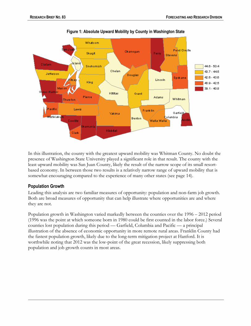
Figure 1: Absolute Upward Mobility by County in Washington State

In this illustration, the county with the greatest upward mobility was Whitman County. No doubt the presence of Washington State University played a significant role in that result. The county with the least upward mobility was San Juan County, likely the result of the narrow scope of its small resort-based economy. In between those two results is a relatively narrow range of upward mobility that is somewhat encouraging compared to the experience of many other states (see page 14).

Population Growth Leading this analysis are two familiar measures of opportunity: population and non-farm job growth. Both are broad measures of opportunity that can help illustrate where opportunities are and where they are not.

Population growth in Washington varied markedly between the counties over the 1996 – 2012 period (1996 was the point at which someone born in 1980 could be first counted in the labor force.) Several counties lost population during this period — Garfield, Columbia and Pacific — a principal illustration of the absence of economic opportunity in more remote rural areas. Franklin County had the fastest population growth, likely due to the long-term mitigation project at Hanford. It is worthwhile noting that 2012 was the low-point of the great recession, likely suppressing both population and job growth counts in most areas.


Figure 2: Population Growth by County in Washington between 1996 and 2012

-10%

0%

10%

20%

30%

40%

50%

60%

70%

80%

90%

Fran

klin

Clar

k

Snoh

omish

Bent

on

Gran

t

Kitt

itas

Wha

tcom

Thur

ston

Mas

on

San

Juan

Doug

las

Pier

ce

Skag

it

King

Skam

ania

Jeffe

rson

Adam

s

Chel

an

Isla

nd

Pend

Ore

ille

Spok

ane

Whi

tman

Yaki

ma

Clal

lam

Stev

ens

Klic

kita

t

Lew

is

Cow

litz

Kits

ap

Wal

la W

alla

Ferr

y

Asot

in

Oka

noga

n

Linc

oln

Wah

kiak

um

Gray

s Har

bor

Paci

fic

Colu

mbi

a

Garf

ield


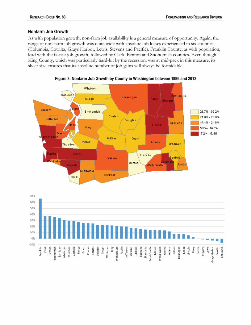
Nonfarm Job Growth As with population growth, non-farm job availability is a general measure of opportunity. Again, the range of non-farm job growth was quite wide with absolute job losses experienced in six counties (Columbia, Cowlitz, Grays Harbor, Lewis, Stevens and Pacific). Franklin County, as with population, lead with the fastest job growth, followed by Clark, Benton and Snohomish counties. Even though King County, which was particularly hard-hit by the recession, was at mid-pack in this measure, its sheer size ensures that its absolute number of job gains will always be formidable.

Figure 3: Nonfarm Job Growth by County in Washington between 1996 and 2012

-10%

0%

10%

20%

30%

40%

50%

60%

70%

Fran

klin

Clar

k

Bent

on

Snoh

omish

San

Juan

Wha

tcom

Thur

ston

Garf

ield

Pier

ce

Gran

t

Chel

an

Kitt

itas

Doug

las

Skag

it

Whi

tman

King

Wah

kiak

um

Asot

in

Jeffe

rson

Klic

kita

t

Clal

lam

Spok

ane

Skam

ania

Pend

Ore

ille

Mas

on

Wal

la W

alla

Yaki

ma

Adam

s

Isla

nd

Oka

noga

n

Kits

ap

Linc

oln

Ferr

y

Paci

fic

Stev

ens

Lew

is

Gray

s Har

bor

Cow

litz

Colu

mbi

a


Population growth and job growth are basic measures of opportunity. And it is apparent that small, remote, rural areas of Washington state have less opportunity in these measures. But this absence of opportunity has consequences beyond the possibility of getting a job, though that is extremely important. Opportunity, or lack thereof, also influences potential income growth — children’s possibility of doing better than their parents. It also hits young men and women differently. In the end, this analysis will illustrate differences in these and other factors, all of which influence AUM — an index of geographic opportunity.

Exposure Effects: Lower Income Growing up in an area of low opportunity can have exposure effects that last over time. Any time spent by a child in an area of low opportunity actually worsens a wide range of socio-economic outcomes in their early years (from college attendance to teenage birth) and on into their adult years (employment and wage progression). The longer the time spent, the worse the long-term outcome.

The following Figure 4 illustrates the exposure effects on the young adult children (age 26) of low income parents (the 25th percentile of the national mean was approximately $30,000). The higher opportunity counties (King, Snohomish, Lincoln and Whitman) generated wages for these young adults anywhere from 9 percent to 15.8 percent above the national mean. Lower opportunity counties (Cowlitz, Grays Harbor, Okanogan and San Juan) produced wages for these young adults that were from 0.8 percent below to 0.5 percent above the national mean.

So it appears that the exposure effects in low opportunity counties on the young adult children of lower income parents were somewhat muted, with only a few counties with young adult income below the national mean.


Figure 4: Exposure Effects for Young Adults Whose Parents Were at the 25th Percentile of National Income

(Gains or losses in income at age 26 relative to the national mean)

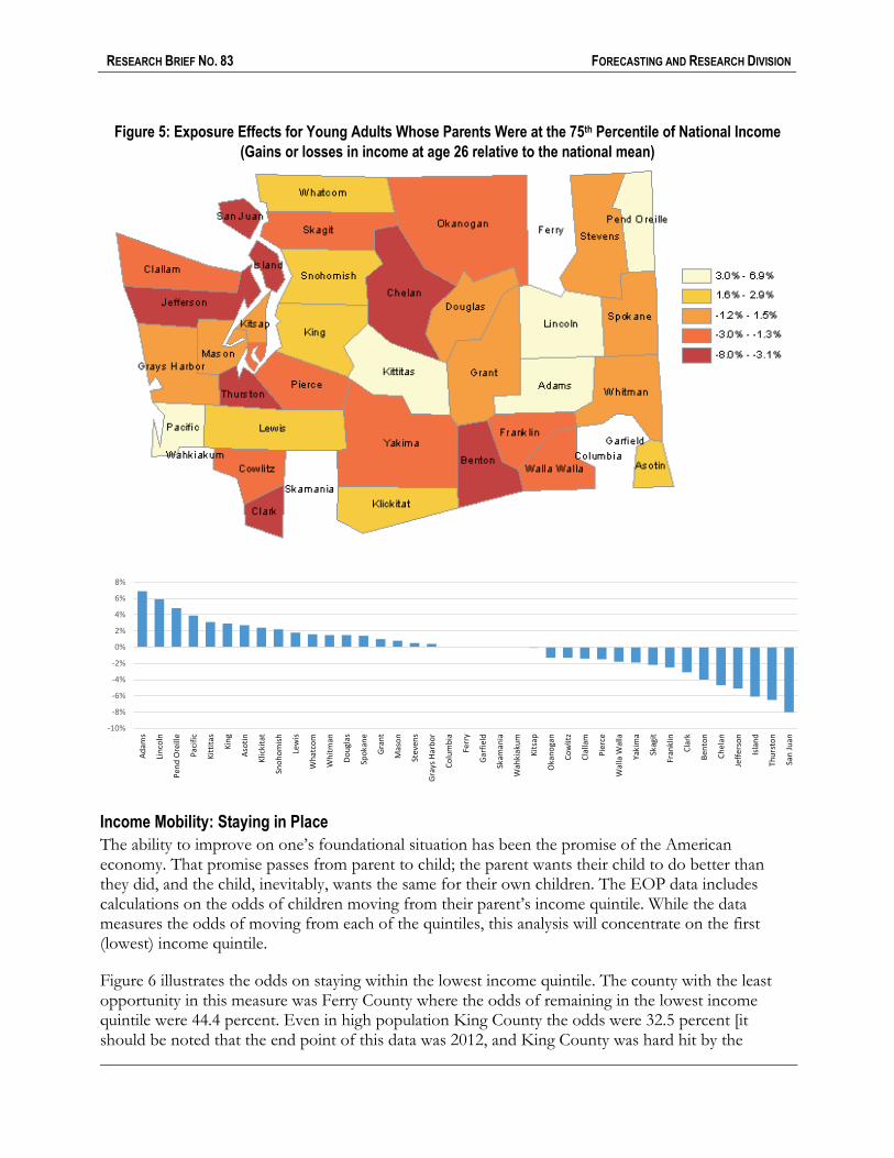
Exposure Effects: Higher Income Exposure effects for the children of higher income parents (the 75th percentile of the national mean was approximately $97,000), in contrast to those of lower income parents, appears much more pronounced. The average wages for the young adult children of higher income parents in 17 lower opportunity counties were below the national mean. Why would children of higher income parents fare worse in areas of low economic opportunity than their low income counterparts? It may be that the labor market expectations for children of higher income parents are unable to be met in low opportunity areas. The lower wage jobs within these geographies may be below their acceptable price-point. It is likely that such a situation would lead to higher levels of out-migration from these low opportunity geographies, particularly among children of higher income parents.

-2%

0%

2%

4%

6%

8%

10%

12%

14%

16%

18%

Whi

tman

Snoh

omish King

Linc

oln

Gran

t

Spok

ane

Kits

ap

Lew

is

Mas

on

Fran

klin

Pend

Ore

ille

Chel

an

Doug

las

Stev

ens

Wal

la W

alla

Kitt

itas

Bent

on

Isla

nd

Thur

ston

Pier

ce

Clal

lam

Wha

tcom

Clar

k

Klic

kita

t

Jeffe

rson

Yaki

ma

Skag

it

Paci

fic

Adam

s

Oka

noga

n

San

Juan

Asot

in

Colu

mbi

a

Ferr

y

Garf

ield

Skam

ania

Wah

kiak

um

Gray

s Har

bor

Cow

litz


Figure 5: Exposure Effects for Young Adults Whose Parents Were at the 75th Percentile of National Income

(Gains or losses in income at age 26 relative to the national mean)

Income Mobility: Staying in Place The ability to improve on one’s foundational situation has been the promise of the American economy. That promise passes from parent to child; the parent wants their child to do better than they did, and the child, inevitably, wants the same for their own children. The EOP data includes calculations on the odds of children moving from their parent’s income quintile. While the data measures the odds of moving from each of the quintiles, this analysis will concentrate on the first (lowest) income quintile.

Figure 6 illustrates the odds on staying within the lowest income quintile. The county with the least opportunity in this measure was Ferry County where the odds of remaining in the lowest income quintile were 44.4 percent. Even in high population King County the odds were 32.5 percent [it should be noted that the end point of this data was 2012, and King County was hard hit by the

-10%

-8%

-6%

-4%

-2%

0%

2%

4%

6%

8%

Adam

s

Linc

oln

Pend

Ore

ille

Paci

fic

Kitt

itas

King

Asot

in

Klic

kita

t

Snoh

omish

Lew

is

Wha

tcom

Whi

tman

Doug

las

Spok

ane

Gran

t

Mas

on

Stev

ens

Gray

s Har

bor

Colu

mbi

a

Ferr

y

Garf

ield

Skam

ania

Wah

kiak

um

Kits

ap

Oka

noga

n

Cow

litz

Clal

lam

Pier

ce

Wal

la W

alla

Yaki

ma

Skag

it

Fran

klin

Clar

k

Bent

on

Chel

an

Jeffe

rson

Isla

nd

Thur

ston

San

Juan


financial crisis emanating from the great recession.] The county with the lowest odds was Adams County at 21.7 percent.

The counties with the highest odds on children of low income parents remaining low-income themselves tend to be more rural, smaller, and economically narrow in scope. The counties with the lowest odds also tended to have similar characteristics, albeit with greater access to interstate highway transportation this easing geographic mobility.

Figure 6: Odds on Staying in the Lowest Income Quintile For Those Whose Parents Were in the Lowest Income Quintile

10%

15%

20%

25%

30%

35%

40%

45%

50%

Ferr

y

Clal

lam

Spok

ane

Cow

litz

Gray

s Har

bor

Clar

k

San

Juan

Thur

ston

Skam

ania

Doug

las

Pier

ce

Jeffe

rson

King

Wha

tcom

Snoh

omish

Kitt

itas

Skag

it

Lew

is

Paci

fic

Kits

ap

Mas

on

Asot

in

Oka

noga

n

Fran

klin

Wal

la W

alla

Stev

ens

Yaki

ma

Whi

tman

Gran

t

Bent

on

Klic

kita

t

Linc

oln

Chel

an

Isla

nd

Pend

Ore

ille

Adam

s

Colu

mbi

a

Garf

ield

Wah

kiak

um


Income Mobility: Reaching the Top Unlike Figure 6, Figure 7 illustrates the odds on the child of low-income, first quintile parents reaching the top income quintile. The odds are greatest in Whitman County at 21.2 percent. This may be due to the fact that Whitman County is home to the main campus of Washington State University. The odds are the lowest in Asotin County, right next door to Whitman County, at 2.4 percent. Apparently the proximity effects are low.

Several Puget Sound counties also exhibited higher potential mobility: King (12.2 percent), Snohomish (12.8 percent), Skagit (11.7 percent), Whatcom (13.2 percent) and San Juan (13.2 percent). Lower potential mobility was found in Clallam (5.5 percent), Ferry (5.6 percent), Jefferson (5.7 percent), Douglas (6.7 percent) and Pend Oreille (8.0 percent).

In each instance, the odds on staying in the lowest quintile exceeded the odds of making it to the top quintile. In Chelan, Klickitat, Pend Oreille and Whitman counties, however, the odds of advancing to the second quintile exceeded the odds of staying in the first.


Figure 7: Odds on Reaching the Top Income Quintile

For Those Whose Parents Were in the Lowest Income Quintile

0%

5%

10%

15%

20%

25%

Whi

tman

Kitt

itas

Bent

on

Wha

tcom

Lew

is

San

Juan

Adam

s

Snoh

omish

Chel

an

Cow

litz

King

Skag

it

Klic

kita

t

Fran

klin

Skam

ania

Oka

noga

n

Kits

ap

Thur

ston

Gran

t

Isla

nd

Stev

ens

Wal

la W

alla

Clar

k

Spok

ane

Linc

oln

Pier

ce

Mas

on

Gray

s Har

bor

Yaki

ma

Paci

fic

Pend

Ore

ille

Doug

las

Jeffe

rson

Ferr

y

Clal

lam

Asot

in

Colu

mbi

a

Garf

ield

Wah

kiak

um


Labor Market Gender Gaps A labor market gender gap is where one gender has a higher ratio of working members than does the other. Nationwide, 69.3 percent of males are in the workforce compared to 57.0 percent of females. That results in a male-female gender gap of 12.3 percentage points. One would expect the gender gap for 30 year olds to be less as marriage and child-raising are more likely in the future. In this analysis a gap with a higher ratio of men will be a number greater than zero, and a gap with a higher ratio of women will be a number less than zero. In the following two figures, counties in which males have higher workforce participation than females are shaded in blue while counties in which females have higher workforce participation than males are shaded in green.

Lower Income Gender Gaps Figure 8 shows several areas where young women from lower-income families tend to have higher workforce participation than similar young men. This occurs both in areas with lower opportunity (Clallam, Grays Harbor, Pacific and Pend Oreille) as well as higher opportunity (King and Whitman). This may illustrate that a poor economy in general and low opportunity areas more specifically are more economically harmful to men from lower-income families than women of similar background.

Figure 8: Employment Gender Gap for Those with Low Income Parents

-25.0%-20.0%-15.0%-10.0%

-5.0%0.0%5.0%

10.0%15.0%20.0%25.0%30.0%

Ferr

y

San

Juan

Skam

ania

Klic

kita

t

Jeffe

rson

Fran

klin

Asot

in

Oka

noga

n

Gran

t

Skag

it

Lew

is

Cow

litz

Stev

ens

Clar

k

Adam

s

Bent

on

Wha

tcom

Wal

la W

alla

Yaki

ma

Chel

an

Spok

ane

Snoh

omish

Colu

mbi

a

Garf

ield

Wah

kiak

um

Pier

ce

King

Kits

ap

Mas

on

Thur

ston

Isla

nd

Clal

lam

Gray

s Har

bor

Kitt

itas

Linc

oln

Doug

las

Whi

tman

Pend

Ore

ille

Paci

fic


Higher Income Gender Gaps Young adult children of higher-income parents have a bit more traditional labor market experience than do those from lower-income parentage, except at the tail-ends of this measure (see Figure 9). With a small area like Skamania County a modest number may have large consequences, so a situation in which 70 percent of young women report earnings and no young men do so should not be too concerning. And at the other end of the gender gap spectrum, Adams County had a gap of 39.1 percent, also likely a product of small numbers. King County, in comparison, had a gender gap of just 5.0 percent, reflective of its size and abundant opportunity. The gap in Klickitat County was -9.9 percent — even though participation was high, young women out-paced young men in workforce activity.

Though of a lesser magnitude than for children of lower-income parents, the gender gap among children of higher-income parents shows that young men are more negatively impacted than young women in areas of low opportunity.

Figure 9: Employment Gender Gap for Those with High Income Parents

-80%

-60%

-40%

-20%

0%

20%

40%

60%

Adam

s

Gran

t

Linc

oln

Pend

Ore

ille

Doug

las

Asot

in

Paci

fic

Cow

litz

Wha

tcom

Gray

s Har

bor

Mas

on

Clar

k

Bent

on

Clal

lam

Skag

it

Fran

klin

Snoh

omish

Spok

ane

Kitt

itas

Pier

ce

King

Lew

is

Kits

ap

Thur

ston

Whi

tman

Ferr

y

Colu

mbi

a

Garf

ield

Wah

kiak

um

Yaki

ma

Wal

la W

alla

Chel

an

Isla

nd

Oka

noga

n

Stev

ens

Jeffe

rson

San

Juan

Klic

kita

t

Skam

ania


Teen Birth Rate The teen birth rate is given weight in this analysis because it illustrates low family stability, a factor correlated to lower economic opportunity. Disparate rates of teen birth appear in close geographic proximity with Whitman County at 5.7 percent and with Franklin County at 20.2 percent (see Figure 10). Adams and Asotin counties also are contiguous to Whitman and also exhibit high teen birth rates of 18.0 percent and 15.9 percent respectively. Again, these are counties of modest size, narrow economic scope, and rural in nature.

The other counties with the lowest teen birth rates were San Juan (5.2 percent), King (7.7 percent), Snohomish (9.5 percent) and Whatcom (9.6 percent). King and Snohomish counties comprise the largest and most diverse metropolitan area in the state which has abundant opportunity. Whatcom County is home to Western Washington University and is proximate to the Canadian city of Vancouver B.C. San Juan County may have a narrow tourism-based economy but is also an enclave of very wealthy households.

Figure 10: Teen Birth Rate

0.0%

5.0%

10.0%

15.0%

20.0%

25.0%

Fran

klin

Yaki

ma

Ferr

y

Gran

t

Adam

s

Skam

ania

Asot

in

Wal

la W

alla

Klic

kita

t

Lew

is

Mas

on

Doug

las

Gray

s Har

bor

Pend

Ore

ille

Oka

noga

n

Stev

ens

Paci

fic

Cow

litz

Chel

an

Bent

on

Skag

it

Clal

lam

Pier

ce

Jeffe

rson

Clar

k

Linc

oln

Spok

ane

Isla

nd

Kits

ap

Kitt

itas

Thur

ston

Wha

tcom

Snoh

omish King

Whi

tman

San

Juan

Colu

mbi

a

Garf

ield

Wah

kiak

um


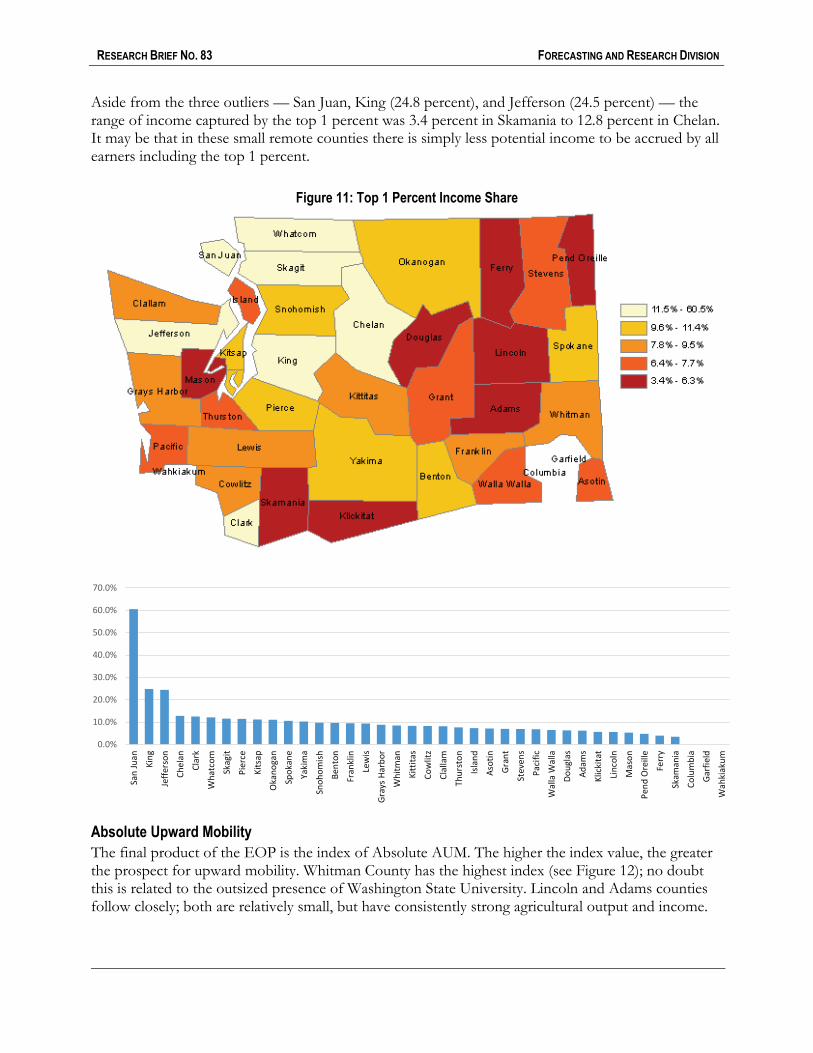
Top 1 Percent Income Share Higher income inequality is supposed to be an indicator of diminished economic mobility. That relationship holds in San Juan County where 60.5 percent of income was captured by the top 1 percent of earners (see Figure 11) and the county has the lowest index of mobility in Washington state (see Figure 12). However, several counties that have a high ratio of income captured by the top 1 percent of earners — Chelan and Jefferson — also have a higher index of upward mobility. In addition, several counties in which there is a low level of income captured by the top 1 percent of earners—Skamania, Klickitat, and Ferry — have a low level of upward mobility.


Aside from the three outliers — San Juan, King (24.8 percent), and Jefferson (24.5 percent) — the range of income captured by the top 1 percent was 3.4 percent in Skamania to 12.8 percent in Chelan. It may be that in these small remote counties there is simply less potential income to be accrued by all earners including the top 1 percent.

Figure 11: Top 1 Percent Income Share

Absolute Upward Mobility The final product of the EOP is the index of Absolute AUM. The higher the index value, the greater the prospect for upward mobility. Whitman County has the highest index (see Figure 12); no doubt this is related to the outsized presence of Washington State University. Lincoln and Adams counties follow closely; both are relatively small, but have consistently strong agricultural output and income.

0.0%

10.0%

20.0%

30.0%

40.0%

50.0%

60.0%

70.0%

San

Juan

King

Jeffe

rson

Chel

an

Clar

k

Wha

tcom

Skag

it

Pier

ce

Kits

ap

Oka

noga

n

Spok

ane

Yaki

ma

Snoh

omish

Bent

on

Fran

klin

Lew

is

Gray

s Har

bor

Whi

tman

Kitt

itas

Cow

litz

Clal

lam

Thur

ston

Isla

nd

Asot

in

Gran

t

Stev

ens

Paci

fic

Wal

la W

alla

Doug

las

Adam

s

Klic

kita

t

Linc

oln

Mas

on

Pend

Ore

ille

Ferr

y

Skam

ania

Colu

mbi

a

Garf

ield

Wah

kiak

um


San Juan County has the least upward mobility in Washington state. Its small size, remoteness, narrow seasonal economy, and a high measure of income inequality are the likely impediments to mobility. Ferry, Skamania, Cowlitz, Asotin, Clallam, Klickitat and Grays Harbor counties are all similarly low on the AUM scale. Each of these counties has similarly narrow economic and remote geographic characteristics.

Washington state has a middling range of upward mobility with county AUM indexes ranging from 39.1 in San Juan to 50.4 in Whitman. The nation had AUM indexes ranging from a low of 26.7 in Mission, South Dakota, to a high of 64.0 in Dickinson, North Dakota (see Figure 13). Washington’s moderate range of upward mobility is likely a function of a high degree of population mobility and the ease of moving to areas of greater opportunity.

Figure 12: Absolute Upward Mobility

30

35

40

45

50

55

Whi

tman

Linc

oln

Adam

s

Kitt

itas

Chel

an

Isla

nd

Bent

on

Pend

Ore

ille

Gran

t

Snoh

omish

Skag

it

Wha

tcom

Jeffe

rson

King

Fran

klin

Doug

las

Wal

la W

alla

Lew

is

Stev

ens

Yaki

ma

Kits

ap

Paci

fic

Thur

ston

Oka

noga

n

Pier

ce

Mas

on

Spok

ane

Clar

k

Gray

s Har

bor

Klic

kita

t

Clal

lam

Asot

in

Cow

litz

Skam

ania

Ferr

y

San

Juan

Colu

mbi

a

Garf

ield

Wah

kiak

um


The National Experience It is apparent from figure 13 that upward mobility varies widely across the U.S. It is also apparent that the degree of mobility is quite constrained in numerous states across the South East. South Carolina has the lowest range of AUM indexes from 34.9 in Bennettsville to 37.7 in Charleston; Charleston being the only area in South Carolina above the lowest decile of mobility.

The state with the widest range of mobility was South Dakota with an AUM index of 26.7 in Mission (primarily the Rosebud Indian Reservation) and 57.6 in Yankton.

North Dakota had the distinction of having only areas in the nation with AUM indexes above 60: Lemmon, Williston, Linton, and Dickinson. This is likely the result of the energy boom that was centered in North Dakota’s Bakken formation, a source of abundant oil and natural gas. While oil and gas exploration has since slowed because of lower oil and energy prices, the region was the center of such activity in 2012.

Figure 13: Absolute Upward Mobility by Commuting Zones in the United States

While the Southeast is generally less income mobile, the plains and Rocky Mountain States are much more upwardly mobile. Of the 13 states that had at least one commuting zone with an AUM index in the top decile, all fell within this central region — none were coastal.

Whether the AUM indexes from the EOP are generally characteristic of the states, commuting zones, and counties, or were a product of the period encompassed by the study remains to be seen. It is expected that the EOP data will be updated in the near future. When that time comes we will have a better understanding of longer-term income mobility.


Studies related to Geographies of Opportunity: George C. Galster and Sean P. Killen, “The Geography of Metropolitan Opportunity: A Reconnaissance and Conceptual Framework,” The Urban Institute, Housing Policy Debate, Volume 6. Issue 1, Fannie Mae 1995.

Xavier de Souza Briggs, “The Geography of Opportunity, Race and Housing Choice in Metropolitan America,” Brookings Institution Press, July, 2005.

Jason Reece, Samir Gambhir, “The Geography of Opportunity, Review of Opportunity Mapping Research Initiatives,” Kirwan Institute for the Study of Race and Ethnicity, the Ohio State University, July 2008.

Sarah Burd-Sharps, Kristen Lewis, “One in Seven, Ranking Youth Disconnection in the 25 Largest Metro Areas,” Measure of America of the Social Science Research Council, September 2012.

Sarah Burd-Sharps, Kristen Lewis, “Geographies of Opportunity, Ranking Well-Being by Congressional District,” Measure of America of the Social Science Research Council, April 2015.

Raj Chetty, Nathaniel Hendren, Patrick Kline, Emmanuel Saez, Nicholas Turner, “Is the U.S. Still a Land of Opportunity? Recent Trends in Intergenerational Mobility,” National Bureau of Economic Research, January 2014.

Raj Chetty, Nathaniel Hendren, Patrick Kline, Emmanuel Saez, “Where is the Land of Opportunity? The Geography of Intergenerational Mobility in the United States,” Harvard University, University of California at Berkeley, National Bureau of Economic Research, June 2014.

Raj Chetty, Nathaniel Hendren, “The impacts of Neighborhoods on Intergenerational Mobility, Childhood Exposure Effects and County-Level Estimates,” Harvard University, April 2015.

Raj Chetty, Nathaniel Hendren, Lawrence Katz, “The effects of Exposure to Better Neighborhoods on Children: New Evidence from the Moving to Opportunity Experiment,” Harvard University, May 2015.

Raj Chetty, Nathaniel Hendren, Frina Lin, Jeremy Majerovitz, Benjamin Scuderi, “Childhood Environment and Gender Gaps in Adulthood,” National Bureau of Economic Research, January 2016.


Source: Equality of Opportunity Project unless otherwise noted

CountyFemale

1stQuintile

Male1st

Quintile

Male-Female1st Quintile

Gap

Female5th

Quintile

Male5th

Quintile

Male-Female5th Quintile

Gap

Parents in 25th Percentile of

National Income

Parents in 75th Percentile of

National Income

1stQuintile

2ndQuintile

3rdQuintile

4thQuintile

5thQuintile

Adams 47.697 0.8108 0.8438 0.0329 0.6087 1.0000 0.3913 1.6% 6.9% 6.2% 18.0% 11.7% 19.3% 0.2174 0.2029 0.2029 0.2464 0.1304

Asotin 40.441 0.6667 0.7647 0.0980 0.8333 0.9600 0.1267 na 2.7% 7.2% 15.9% 20.1% 7.9% 0.2927 0.2439 0.2195 0.2195 0.0244

Benton 45.247 0.7021 0.7348 0.0327 0.7877 0.8709 0.0832 3.9% -4.0% 9.6% 13.5% 36.8% 34.3% 0.2564 0.2234 0.2381 0.1392 0.1429

Chelan 45.483 0.7979 0.8137 0.0159 0.8523 0.8450 -0.0074 5.7% -4.7% 12.8% 13.8% 25.4% 18.6% 0.2245 0.2296 0.2092 0.2092 0.1276

Clallam 40.448 0.6768 0.6471 -0.0297 0.8065 0.8889 0.0824 3.6% -1.4% 8.2% 13.0% 17.1% 14.2% 0.3807 0.1972 0.1651 0.2018 0.0550

Clark 41.925 0.6183 0.6589 0.0405 0.7722 0.8577 0.0855 3.2% -3.1% 12.5% 12.1% 37.0% 42.2% 0.3422 0.1962 0.2166 0.1460 0.0989

Columbia na na na na na na na na na 0.0% 0.0% -7.2% -4.2% na na na na na

Cowlitz 40.430 0.6617 0.7063 0.0447 0.7680 0.8735 0.1055 -0.8% -1.3% 8.2% 13.9% -4.3% 12.7% 0.3707 0.1969 0.1583 0.1506 0.1236

Douglas 43.572 0.8000 0.6400 -0.1600 0.7800 0.9242 0.1442 5.7% 1.5% 6.3% 14.9% 22.7% 25.3% 0.3333 0.1778 0.2222 0.2000 0.0667

Ferry 40.028 0.5263 0.7647 0.2384 na na na na na 4.0% 18.6% 3.0% 8.4% 0.4444 0.1111 0.1944 0.1944 0.0556

Franklin 43.600 0.7286 0.8352 0.1066 0.8101 0.8737 0.0636 5.9% -2.5% 9.5% 20.2% 66.2% 87.5% 0.2857 0.2609 0.2050 0.1366 0.1118

Garfield na na na na na na na na na 0.0% 0.0% 28.6% -5.2% na na na na na

Grant 44.368 0.7357 0.8116 0.0759 0.7045 0.9279 0.2234 8.9% 1.0% 7.0% 18.5% 25.7% 34.0% 0.2662 0.2302 0.2446 0.1511 0.1079

Grays Harbor 40.828 0.6442 0.6107 -0.0334 0.7677 0.8660 0.0983 -0.5% 0.4% 8.9% 14.8% -3.2% 5.8% 0.3686 0.2212 0.1923 0.1346 0.0833

Island 45.318 0.7636 0.7368 -0.0268 0.8468 0.8273 -0.0196 3.9% -6.1% 7.3% 10.9% 7.5% 18.1% 0.2232 0.1786 0.2500 0.2411 0.1071

Jefferson 44.054 0.6471 0.8056 0.1585 0.8718 0.8222 -0.0496 2.6% -5.1% 24.5% 12.4% 19.9% 20.6% 0.3286 0.2000 0.1857 0.2286 0.0571

King 43.796 0.6783 0.6764 -0.0020 0.8098 0.8601 0.0503 11.3% 2.9% 24.8% 7.7% 21.8% 21.4% 0.3254 0.2032 0.2022 0.1474 0.1218

Kitsap 42.730 0.6985 0.6860 -0.0125 0.8185 0.8633 0.0448 7.1% -0.1% 11.2% 10.8% 7.1% 12.4% 0.2980 0.2537 0.2020 0.1355 0.1108

Kittitas 46.479 0.8158 0.7632 -0.0526 0.7857 0.8438 0.0580 4.1% 3.1% 8.3% 10.5% 25.0% 32.3% 0.3158 0.1842 0.1316 0.2237 0.1447

Klickitat 40.580 0.6552 0.8333 0.1782 0.8889 0.7895 -0.0994 3.2% 2.4% 5.7% 15.3% 17.9% 13.7% 0.2453 0.2830 0.2453 0.1132 0.1132

Lewis 43.373 0.6850 0.7304 0.0454 0.7787 0.8258 0.0471 6.3% 1.8% 9.4% 15.2% -2.6% 13.5% 0.3099 0.1736 0.1860 0.1983 0.1322

Lincoln 48.446 0.8333 0.7000 -0.1333 0.6923 0.8824 0.1900 11.3% 5.9% 5.6% 12.0% 5.4% 6.5% 0.2273 0.1364 0.3636 0.1818 0.0909

Mason 41.927 0.7069 0.6885 -0.0184 0.7656 0.8514 0.0857 6.1% 0.8% 5.3% 15.0% 14.0% 28.4% 0.2941 0.2605 0.1513 0.2101 0.0840

Okanogan 42.046 0.6750 0.7589 0.0839 0.9268 0.8909 -0.0359 0.5% -1.3% 11.1% 14.4% 7.5% 7.0% 0.2874 0.2567 0.2069 0.1379 0.1111

Pacific 42.474 0.7941 0.5854 -0.2088 0.7931 0.9167 0.1236 1.9% 3.9% 6.8% 14.1% -0.6% -2.5% 0.3067 0.2400 0.2000 0.1733 0.0800

Pend Oreille 44.547 0.7600 0.5600 -0.2000 0.8125 1.0000 0.1875 5.9% 4.8% 4.7% 14.8% 14.0% 16.8% 0.2200 0.2400 0.2200 0.2400 0.0800

Pierce 41.995 0.6862 0.6843 -0.0019 0.8045 0.8584 0.0539 3.8% -1.5% 11.4% 12.6% 27.4% 23.8% 0.3296 0.2125 0.2045 0.1636 0.0898

San Juan 39.103 0.6250 0.8571 0.2321 0.7778 0.7143 -0.0635 0.5% -8.0% 60.5% 5.2% 34.2% 26.1% 0.3421 0.2368 0.1316 0.1579 0.1316

Skagit 44.158 0.6429 0.6903 0.0475 0.8072 0.8853 0.0781 2.1% -2.2% 11.6% 13.4% 22.1% 23.3% 0.3107 0.1974 0.2136 0.1618 0.1165

Skamania 40.211 0.7273 0.9375 0.2102 0.7000 na -0.7000 na na 3.4% 16.9% 14.9% 21.1% 0.3333 0.1852 0.2593 0.1111 0.1111

Snohomish 44.182 0.6524 0.6621 0.0097 0.7965 0.8597 0.0632 14.4% 2.2% 9.7% 9.5% 35.8% 34.3% 0.3175 0.1892 0.1958 0.1692 0.1283

Spokane 41.926 0.6632 0.6767 0.0135 0.8037 0.8667 0.0630 8.9% 1.4% 10.6% 11.4% 16.1% 16.5% 0.3707 0.2149 0.1741 0.1471 0.0932

Stevens 43.022 0.6957 0.7386 0.0430 0.8500 0.8085 -0.0415 5.0% 0.5% 6.9% 14.2% -1.4% 13.8% 0.2778 0.2278 0.2278 0.1611 0.1056

Thurston 42.180 0.7100 0.6853 -0.0246 0.8196 0.8532 0.0336 3.9% -6.5% 7.7% 10.3% 28.8% 31.8% 0.3369 0.1987 0.1901 0.1663 0.1080

Wahkiakum na na na na na na na na na 0.0% 0.0% 20.8% 5.8% na na na na na

Walla Walla 43.522 0.6667 0.6897 0.0230 0.8660 0.8636 -0.0023 4.9% -1.8% 6.5% 15.4% 13.7% 9.9% 0.2782 0.2406 0.2030 0.1729 0.1053

Whatcom 44.127 0.6606 0.6844 0.0238 0.7669 0.8655 0.0986 3.6% 1.6% 12.2% 9.6% 30.7% 32.0% 0.3184 0.1794 0.2354 0.1345 0.1323

Whitman 50.365 0.9565 0.7586 -0.1979 0.8814 0.8909 0.0096 15.8% 1.5% 8.5% 5.7% 21.9% 15.2% 0.2692 0.3462 0.0769 0.0962 0.2115

Yakima 42.873 0.7396 0.7556 0.0159 0.8231 0.8214 -0.0016 2.5% -1.9% 10.3% 20.0% 13.6% 14.8% 0.2757 0.2350 0.2427 0.1644 0.08221 Washington State Employment Security Department2 Washington State Office of Financial Management

Difference in Income for Those WithWork force participation at age 30 by gender and parent income quintile Probability of Income for Those Whose Parents were in the 1st Quintile

Geographies of Opportunity Map Data for Washington Counties

Top 1%IncomeShare

TeenBirthRate

Nonfarm Employment

Growth1

Population Growth2

Absolute Upward Mobility

Documents

WASHINGTON STATE OFFICE OF FINANCIAL MANAGEMENT · 2019-12-11 · WASHINGTON STATE OFFICE OF FINANCIAL MANAGEMENT WASHINGTON ECONOMIC TRENDS Research Brief No. 83 March 2017 Geographies