Was Prometheus Unbound by Chance? Risk, …econdse.org/wp-content/uploads/2015/10/AcemogluZillibotiJPE97.pdf · Was Prometheus Unbound by Chance? Risk, Diversification, and Growth

Was Prometheus Unbound by Chance? Risk, Diversification, and Growth

Daron Acemoglu; Fabrizio Zilibotti

The Journal of Political Economy, Vol. 105, No. 4. (Aug., 1997), pp. 709-751.

Stable URL:

http://links.jstor.org/sici?sici=0022-3808%28199708%29105%3A4%3C709%3AWPUBCR%3E2.0.CO%3B2-%23

The Journal of Political Economy is currently published by The University of Chicago Press.

Your use of the JSTOR archive indicates your acceptance of JSTOR's Terms and Conditions of Use, available athttp://www.jstor.org/about/terms.html. JSTOR's Terms and Conditions of Use provides, in part, that unless you have obtainedprior permission, you may not download an entire issue of a journal or multiple copies of articles, and you may use content inthe JSTOR archive only for your personal, non-commercial use.

Please contact the publisher regarding any further use of this work. Publisher contact information may be obtained athttp://www.jstor.org/journals/ucpress.html.

Each copy of any part of a JSTOR transmission must contain the same copyright notice that appears on the screen or printedpage of such transmission.

The JSTOR Archive is a trusted digital repository providing for long-term preservation and access to leading academicjournals and scholarly literature from around the world. The Archive is supported by libraries, scholarly societies, publishers,and foundations. It is an initiative of JSTOR, a not-for-profit organization with a mission to help the scholarly community takeadvantage of advances in technology. For more information regarding JSTOR, please contact [email protected].

http://www.jstor.orgSun Jul 29 18:34:09 2007


http://www.jstor.org/about/terms.html

http://www.jstor.org/journals/ucpress.html

Was Prometheus Unbound by Chance? Risk, Diversification, and Growth

Daron Acemoglu 12.Iassachusetts Institute of Trchnologi

Fabrizio Zilibotti CTniversitat Pon~peu Fabra

This paper offers a theory of development that links the degree of market incompleteness to capital accumulation and growth. At early stages of development, the presence of indivisible projects limits the degree of risk spreading (diversification) that the economy can achieve. The desire to avoid highly risky investments slows down capital accumulation, and the inability to diversifj idiosyncratic risk introduces a large amount of uncertainty in the growth process. The typical development pattern will consist of a lengthy period of "primitive accumulation" with highly variable output, followed by takeoff and financial deepening and, finally, steady growth. "Lucky" countries will spend relatively less time in the primitive accumulation stage and develop faster. Although all agents are price takers and there are no technological spillovers, the decentralized equilibrium is inefficient because individuals do not take into account their impact on others' diversification opportunities. We also show that our results generalize to economies with international capital flows.

We are grateful to Dudley Baines, Abhijit Banerjee, Andrew Bernard, Alberto Bisin, Peter Diamond, Jordi Gali, Hugo Hopenhayn, Albert Marcet, Andreu Mas- Colell, Thomas Piketty, Sherwin Rosen, Julio Rotemberg, Xavier Sala-i-Martin, h-drew Scott, and Jaume Ventura; to various seminar participants; and especially to an anonymous referee for useful comments. Financial support from the Ministry of Education of Spain (DGICYT PB93-0388) is acknowledged.

[Journal oJPolitica1 Economy, 1997, vol. 105, no. 41 O 1997 by The LTn~rersity of Chicago. MI rights resened. 0022-3808/97/0~04-0001$02.j0

71° JOURNAL OF POLITICAL ECONOMY

I. Introduction

The advance occurred very slowly over a long period and was broken by sharp recessions. The right road was reached and thereafter never abandoned, only during the eighteenth century, and then only by a few privileged countries. Thus, before 1750 or even 1800 the march of progress could still be affected by unex- pected events, even disasters. [Braudel 1973, p. xi]

This view of slow and uncertain progress between the tenth and early nineteenth centuries is shared by many economic historians. North and Thomas (1973, p. 71) describe the fourteenth and fifteenth centuries as times of "contractions, crisis and depression," and DeVries (1976) refers to this period as "an Age of Crisis." The same phenom- enon is observed today: Lucas (1988, p. 4) writes that whereas "within the advanced countries, growth rates tend to be very stable over long periods of time," for poorer countries, "there are many examples of sudden, large changes in growth rates, both up and down." Why are the early stages of development slow and subject to so much randomness? Models of economic development based on threshold effects (e.g., Azariadis and Drazen 1990) may be modified to predict a slow development process, but even then, these models have no implications regarding randomness of growth. In contrast, this paper argues that these patterns are predicted by the neoclassical growth model augmented with the natural assumptions of micro-level indivisibilities and micro-level uncertainty.

U7e begin with a number of observations that will be elaborated and empirically supported in the next section. First, most economies have access to a large number of imperfectly correlated projects; thus a significant part of the risks they face can be diversified. Sec- ond, a large proportion of these projects are subject to significant indivisibilities, especially in the form of minimum size requirements or start-up costs. Third, agents dislike risk. Fourth, there exist less productive but relatively safe investment opportunities. And finally, societies at the early stages of development have less capital to invest than developed countries. These features lead to a number of important implications. (i) At the early stages of development, owing to the scarcity of capital, only a limited number of imperfectly correlated projects can be undertaken, and agents will seek insurance by investing in safe but less productive assets. As a result, poor countries will endogenously have lower productivity, and this will contribute to their slow development. (ii) Since the diversification opportunities are limited, existing activities will bear more of the diversifiable risks. This will make the earlier stages of development highly ran-

711 RISK, DIVERSIFICATION, GROWTH

dom and slow down economic progress further since many runs toward takeoff will be stopped by crises. (iii) Chance will play a very important role; economies that are lucky enough to receive good draws at the early stages will have more capital and thus will achieve better risk diversification and higher productivity. Therefore, although Prometheus will not be unbound accidentally, chance will always play a key role in his unchaining.

In our model, agents decide how much to save and how much of their money to invest in a safe asset with lower return. The rest of the funds are used to invest in imperfectly correlated risky projects. However, not all risky projects are available to agents at all points in time because of the minimum size requirements that affect some of these sectors. The more "sectors" (projects) that are open, the higher the proportion of their savings that agents are willing to put in risky investments. In turn, when the capital stock of the economy is larger, there will be more savings, and more sectors can be opened. Therefore, development goes hand in hand with the expansion of markets and with better diversification opportunities. Never- theless, this process is full of perils because with limited investments in imperfectly correlated projects, the economy is subject to considerable randomness and spends a long time fluctuating in the stage of low accumulated capital. Only economies that receive "lucky draws" will grow, whereas those that are unfortunate enough to receive a series of "bad news" will stagnate. As lucky economies grow, the takeoff stage will be reached eventually, and full diversification of idiosyncratic risks will be achieved.

Theoretically, our model corresponds to an economy with endogenous commodity space because the set of traded financial assets (or open sectors) is determined in equilibrium. We use the competitive equilibrium concept suggested by Hart (1979) and Makowski (1980) for this type of economy. This equilibrium is Walrasian conditional on the set of sectors that are open, and the number of open sectors is determined through a free-enuy condition. Although all agents are price takers and there are no unexploited gains in any activity, the competitive equilibrium is inefficient and too few projects are undertaken. The underlying problem is that the opening of an additional sector creates a positive pecuniary externality on other open projects since consumers now bear less risk when they buy these securities. Not only do we show that the competitive equilibrium is inefficient, but we establish the stronger result that under plausible assumptions on commitment, there exists no decentralized market structure that can avoid this inefficiency.

It may be conjectured that since our mechanism is related to capital shortages, its validity will be limited in the presence of interna-

712 JOURNAL OF POLITICAL ECONOMY

tional capital flows. In Section V, we show that decreasing return to capital would make foreign funds flow toward poor economies. But counteracting this, better insurance opportunities in richer countries could make domestic capital flow out. In a two-country general- ization of our model, these forces lead to an interesting pattern that matches the historical facts of Western European development: At the early stages, funds flow into one of the countries; thus capital flows create divergence. But as the world economy becomes richer, the direction of capital flows is reversed, and there is rapid convergence (see Neal 1990).

Our model is related to the growing literature on credit and growth (among others, Greenwood and Jovanovic [1990], Benci- venga and Smith [1991], Saint-Paul [1992], Greenwood and Smith [1993], and Zilibotti [1994]). Like these papers, our work shows that capital accumulation is associated with an increase in the volume of intermediation and financial activities as a proportion of the gross domestic product (see the empirical findings of Goldsmith [1969], Atje and Jovanovic [1993], and King and Levine [1993]). However, while most existing theories derive their dynamics from the presence of fixed costs of financial intermediation, in our model there are no explicit costs of financial relations. Instead, all costs arise endogenously because of the diversification efforts of agents. We show that better diversification opportunities enable a gradual allocation of funds to their most productive uses while reducing the variability of growth. The intuition that risk diversification will lead to more productive specialization was first expressed by Gurley and Shaw (1955) and is modeled in Saint-Paul (1992). Greenwood and Jo- vanovic (1990) also show that the variability of growth may decrease with development. Our paper differs from these contributions because the degree of diversification and the extent of market incompleteness in the aggregate economy are endogenized and because there are no exogenous costs of financial intermediation. Further, the inefficiency of equilibrium with price-taking agents and the links between credit markets and international capital flows are also novel.

Another important literature that relates to our work is the one pioneered by Townsend (1978, 1983), Boyd and Prescott (1986), and Allen and Gale (1988, 1991), which studies financing decisions in general equilibrium. As in Allen and Gale, we endogenize the market structure, but without explicit costs of issuing securities. Fur- thermore, we focus mainly on the interaction between the incompleteness of markets, the opportunities for diversification, and the process of development. We follow the work of Townsend and others in allowing coalitions to internalize financial externalities. However,

RISK, DIVERSIFICATION, GROWTH 7 l 3

in contrast to these papers, we show that the efficient allocation is extremely hard to sustain as a decentralized equilibrium. The reason for these different conclusions will be explained in Section V.

The paper is organized as follows. Section I11 lays out the basic model and characterizes the equilibrium. Section IV shows that the decentralized equilibrium is not Pareto-efficient and characterizes the Pareto-optimal allocation. Section V demonstrates that the inefficiency result is robust to the formation of financial coalitions. Sec- tion VI analyzes international capital flows, and Section VII presents a conclusion.

11. Motivation and Historical Evidence

Many economic historians (e.g., Braudel 1973, 1982; North and Thomas 1973; DeVries 1976) emphasize the high variability of performance at the early stages of development. McCloskey (1976) cal- culates that the coefficient of variation of output net of seed in medieval England was 0.347 and that "famines" were occurring on average every 13 years. Part of this variability is certainly due to the fact that agricultural productivity was largely dependent on weather. But this heavy reliance on agriculture is itself a symptom of an undiversified economy. Additionally, there is considerable evidence that nonagricultural activities were also subject to large uncertainties. Braudel describes the development of industry before 1750 as "subject to halts and breakdowns" (1982, p. 312). He points out the presence of failed takeoffs: "three occasions in the West when there was an expansion of banking and credit so abnormal as to be visible to the naked eye [Florence 1300s, Genoa late 1500s, and Amsterdam 1700~1. . . three substantial successes, which ended every time in failure or at any rate in some kind of withdrawal" (p. 392). The pattern of these failures is also informative. While these cities grew gradually by expanding the scope of industrial and commercial activities, the collapse took the form of an abrupt end ignited by a few bankruptcies, suggesting the presence of large undiversified risks.

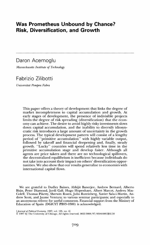
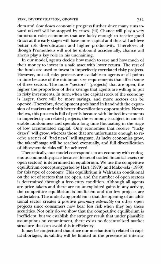
Poor countries today also exhibit considerably higher variability of output than more developed economies. Figure 1 plots the loga- rithm of the standard deviation of each country's GDP per capita growth rate over the period 1960-85 versus the GDP per capita in 1960 for 117 countries from the data set in Summers and Heston (1991). The solid curve traces the regression line, calculated exclud- ing Saudi Arabia, a rich country with highly volatile growth due to oil prices. This line has a negative and highly significant coefficient (t-statistic, -6.68) and an R2of .29. When we drop five outliers (Iran, Iraq, Gabon, Somalia, and Uganda) for which political unrest and

JOURNAL OF POLITICAL ECONOMY

FIG. 1.-Variability of growth

wars appear to have been the main source of their exceptionally high variability, the fit of the regression increases to R2 = .34.A 1percent increase in the initial GDP is associated, on average, with a 0.25 percent decrease in the standard deviation of growth, a very large quan- titative effect.

Similar results are obtained by pooling cross-sectional and time- series information. We consider pairs of observations {GDP,,,, IE,,~,,~}, where 1 ~ , + , , , 1 is the absolute value of the one-period-ahead deviation from the average growth rate in country i . We then divide our 117 X 25 pairs of observations into four groups according to increasing GDP per capita ranges (XI = [O, 7001, X2 = [700, 1,5001, X3 = [1,500, 4,5001, and z4= [4,500, m]) and assign each deviation to -one group so that { 1 ~ , * , , * + ~ 1 ) E {GROUPk}if and only if GDP,*,,* E X , (GDP per capita in 1980 U.S. dollars). Finally, we compute the sample mean for the (pooled) absolute value of deviations in each group. The results are reported in table 1, with the standard error of the mean in parentheses. Column 1 shows that the average size of deviation from the mean growth rate decreases with the income range; hence a low-income country or period is associated with higher variability. In column 2 (with fixed effects), we report the sample means for the corresponding income ranges after control- ling for fixed country and time effects by subtracting from each observation the respective country and time means (averaged, respectively, across t and i) . Since we are computing deviations from averages, some observations will now be negative. The negative correlation between GDP levels and growth variability remains very sig-

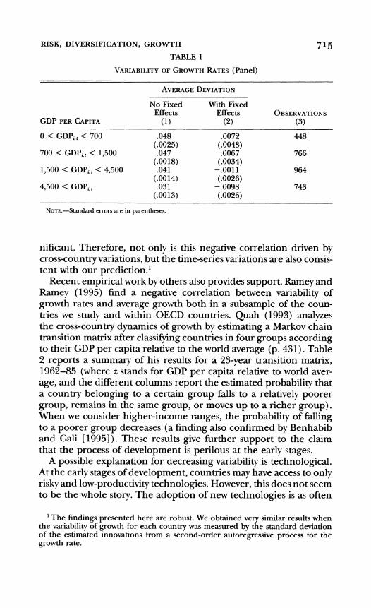
RISK, DIVERSIFICATION, GROWTH 7 l5 TABLE 1

VARIABILITY RATESOF GROWTH (Panel)

No Fixed With Fixed

GDP PER CAPITA Effects

(1) Effects

(2) OBSERVATIONS

(3)

0 < GDP,,,< 700

700 < GDP,, < 1,500

.048 (.0025) .047

4,500 < GDP,,

NOTE.-Standard errors are in parentheses.

nificant. Therefore, not only is this negative correlation driven by cross-country variations, but the time-series variations are also consistent with our prediction.'

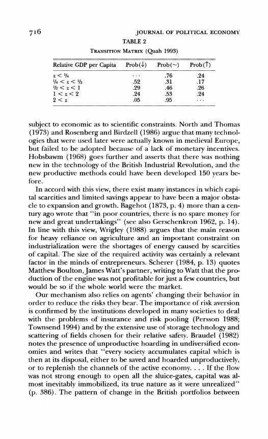
Recent empirical work by others also provides support. Ramey and Ramey (1995) find a negative correlation between variability of growth rates and average growth both in a subsample of the countries we study and within OECD countries. Quah (1993) analyzes the cross-country dynamics of growth by estimating a Markov chain transition matrix after classifying countries in four groups according to their GDP per capita relative to the world average (p. 431). Table 2 reports a summary of his results for a 23-year transition matrix, 1962-85 (where z stands for GDP per capita relative to world average, and the different columns report the estimated probability that a country belonging to a certain group falls to a relatively poorer group, remains in the same group, or moves up to a richer group). When we consider higher-income ranges, the probability of falling to a poorer group decreases (a finding also confirmed by Benhabib and Gali [1995]). These results give further support to the claim that the process of development is perilous at the early stages.

A possible explanation for decreasing variability is technological. At the early stages of development, countries may have access to only risky and low-productivity technologies. However, this does not seem to be the whole story. The adoption of new technologies is as often

'The findings presented here are robust. We obtained very similar results when the variability of growth for each country was measured by the standard deviation of the estimated innovations from a second-order autoregressive process for the growth rate.


TABLE 2

TRANSITION (Quah 1993)MATRIX

Relative GDP per Capita rob (J) Prob (-) rob (T)

subject to economic as to scientific constraints. North and Thomas (1973) and Rosenberg and Birdzell (1986) argue that many technologies that were used later were actually known in medieval Europe, but failed to be adopted because of a lack of monetary incentives. Hobsbawm (1968) goes further and asserts that there was nothing new in the technology of the British Industrial Revolution, and the new productive methods could have been developed 150 years before.

In accord with this view, there exist many instances in which capital scarcities and limited savings appear to have been a major obsta- cle to expansion and growth. Bagehot (1873, p. 4) more than a century ago wrote that "in poor countries, there is no spare money for new and great undertakings" (see also Gerschenkron 1962, p. 14). In line with this view, Wrigley (1988) argues that the main reason for heavy reliance on agriculture and an important constraint on industrialization were the shortages of energy caused by scarcities of capital. The size of the required activity was certainly a relevant factor in the minds of entrepreneurs. Scherer (1984, p. 13) quotes Matthew Boulton, James Watt's partner, writing to Watt that the production of the engine was not profitable for just a few countries, but would be so if the whole world were the market.

Our mechanism also relies on agents' changing their behavior in order to reduce the risks they bear. The importance of risk aversion is confirmed by the institutions developed in many societies to deal with the problems of insurance and risk pooling (Persson 1988; Townsend 1994) and by the extensive use of storage technology and scattering of fields chosen for their relative safety. Braudel (1982) notes the presence of unproductive hoarding in undiversified economies and writes that "every society accumulates capital which is then at its disposal, either to be saved and hoarded unproductively, or to replenish the channels of the active economy. . . . If the flow was not strong enough to open all the sluice-gates, capital was almost inevitably immobilized, its true nature as it were unrealized" (p. 386). The pattern of change in the British portfolios between

RISK, DIVERSIFICATION, GROWTH 7 l7

the eighteenth and nineteenth centuries also documents that as per capita income increased, the use of relatively safe assets decreased and the array of available assets expanded considerably (see Ken- nedy 1987, table 5.1).

Finally, this paper stresses that lack of diversification at early stages of development leads to an important role of "chance," especially regarding the success of large and risky projects. In this context, the impact of railways on economic development is interesting. In the United States, the success of railways is hailed as opening the way for the financing of large projects (e.g., Chandler 1977), whereas in Spain, where railways attracted 15 times as much capital as total manufacturing, the heavy losses on railway investments are argued to have led to serious capital scarcities for decades (Tortella 1972, pp. 118-21). Regarding this episode and a similar one in Italy, Cam- eron (1972, p. 14) writes that "in both cases the result was a fiasco which set back the progress of industrialization and economic development by at least a generation."

111. The Model and the Decentralized Equilibrium

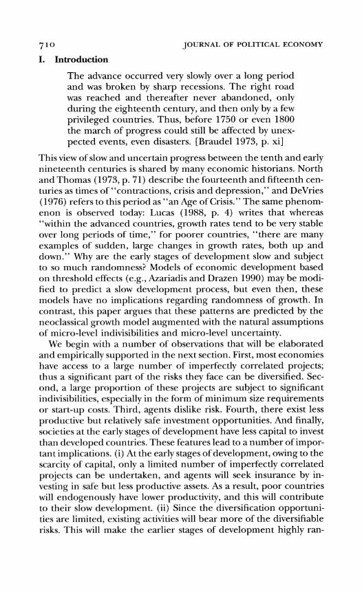
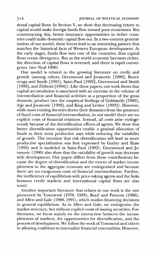
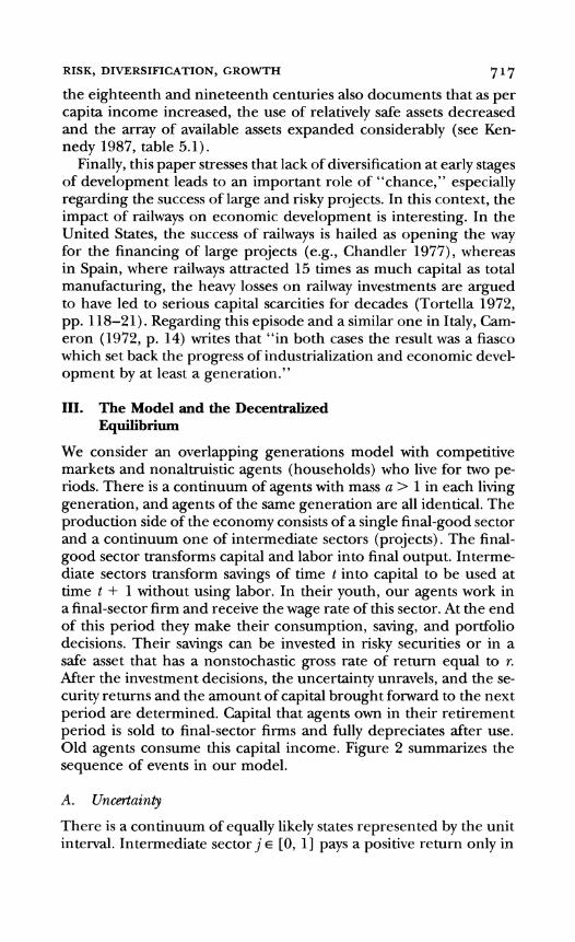
We consider an overlapping generations model with competitive markets and nonaltruistic agents (households) who live for two periods. There is a continuum of agents with mass a > l in each living generation, and agents of the same generation are all identical. The production side of the economy consists of a single final-good sector and a continuum one of intermediate sectors (projects). The final- good sector transforms capital and labor into final output. Interme- diate sectors transform savings of time t into capital to be used at time t + 1 without using labor. In their youth, our agents work in a final-sector firm and receive the wage rate of this sector. At the end of this period they make their consumption, saving, and portfolio decisions. Their savings can be invested in risky securities or in a safe asset that has a nonstochastic gross rate of return equal to r. After the investment decisions, the uncertainty unravels, and the security returns and the amount of capital brought forward to the next period are determined. Capital that agents own in their retirement period is sold to final-sector firms and fully depreciates after use. Old agents consume this capital income. Figure 2 summarizes the sequence of events in our model.

A. Uncertainty

There is a continuum of equally likely states represented by the unit interval. Intermediate sector j E [O, I ] pays a positive return only in

7 18 JOURNAL OF POLITICAL ECONOMY

YOUNG Riskless asset ( O t ) I OLD

k

Risky assets {F;]

Wag. ( w r )

conevrnpt,on (c,)

FIG.2.-Timing of events (j,stands for the realized state of nature)

state jand nothing in any other state. Therefore, investing in a sector is equivalent to buying a basic Arrow security that pays in only one state of nature. More formally, an investment of FJin sector j pays the amount RFJ if state j occurs and FJ2 Mj, and nothing otherwise. In our model, R > r, so these projects are more productive than the safe investment. The requirement FJ2MI implies that all intermediate sectors have linear technologies, but some require a certain minimum size, MI, before being productive. The distribution of minimum size requirements is given by

DM, = max10, --(1-1)).

1 - Y Sectors j 5 y have no minimum size requirement, and for the rest of the sectors, the minimum size requirement increases linearly (see fig. 3 below for a diagrammatic representation). The results are not dependent on this linear specification, and the ranking of projects from lower to higher size occurs without loss of generality and im- poses no timing constraint.

This formalization contains the two features that will drive our results: (i) risky investments have a higher expected return than the safe asset (i.e., R > r) , and (ii) different projects are imperfectly correlated so that there is safety in variety. A convenient implication of this formulation is that if a portfolio consists of an equipropor- tional investment F in all projects j E J C [0, 11 and the measure of the set is p, then the portfolio pays the return RFwith probability p and nothing with probability 1 - p. Note that if the aggregate

RISK, DIVERSIFICATION, GROWTH 7 l 9

production set were convex (i.e., D = O ) , the allocation problem of the economy would be trivial: all agents would invest an equal amount in all intermediate goods sectors and diversify all the risks. However, in the presence of nonconvexities, as captured by our minimum size requirements, there is a trade-off between insurance and high productivity.

B. Preferences, Technology, and Factor Prices

The preferences of consumers over final goods are defined as

where jrepresents the states of nature, which are assumed, as noted above, to be equally likely. Each agent discounts the future at the rate p and has a rate of relative risk aversion equal to one. Although the realization of the state of nature does not influence the productivity of the final-good sector, it affects consumption since it deter- mines how much capital each agent takes into the final-good production stage and the equilibrium price of capital.

Output of the final-good sector is given by

We normalize the labor endowment of each young worker to 1/ a . Since the mass of agents is a and labor supply is inelastic, we have L, = 1. The aggregate stock of capital depends on the realization of the state of nature. If the state of nature is j, then K',,, =

In,(r@,,,+ RFj, , ,)dh,where F',,, is the amount of savings invested by agent h E Q, in sector j, @,,,,is the amount invested in the safe asset, and R, is the set of young agents at time t. Since both labor and capital trade in competitive markets, equilibrium factor prices in state j are given as

and

The wage earning of a young agent conditional on the realization of state j will then be w', = W { / a .

72o JOURNAL OF POLITICAL ECONOMY

C. Intermediate Goods and Portfolio Decisions

We assume that intermediate sector firms are run by agents who compete to get funds by issuing financial securities and sell them to other agents in the stock market. Each agent can run at most one project, although more than one agent can compete to run the same project (see Sec. V for generalizations).

Decisions are made in two stage^.^ In the first stage, each agent h E R, takes the announcements of all other agents as given and announces his plan to run at most one project in the intermediate sector and sell an unlimited quantity of the associated basic Arrow security. Securities are labeled by the indices of the project to which they are attached. Therefore, one unit of security j entitles its holder to R units of t + 1 capital in state of nature j. We denote the unit price of security j (in terms of savings of time t) by P,h,t ,and subscript h implies that this security is issued by agent h. Put differently, agent h is managing investments in project j on behalf of other agents, and for every unit of savings he collects from others, he invests 1/ P , , ,and keeps the remaining (P,,,, , - 1)/P,.,,,as his commission. A first-stage strategy for agent h at time t is an announcement Z,, , = (j, P,,,,,) E [0, 11 X R specifying the project h intends to run and +

the price at which he sells the corresponding security. If an agent h' decides to run no project, then Zh,,, = 0.The function Z,:R, + [O, 11 X R + summarizes the announcements of all agents at time t. We also denote the subset of all projects that at least one agent pro- poses to run at time t by J,(Z,) G [O, 11; thusJ,(Z,) = { jE [O, 11 I 3 h s.t. Zh,, = Finally, we define P,(Z,) :J,(Z,) + R f as the (1,P,,,,,)}. function that summarizes the minimum price for each security j E

J,(Z,) induced by the set of announcements 2,. Formally, P,(Z,) =

{pJ(Zt)}l~l = minihst Z h t = ( l , P , , ) I ( 4 . h f). On, the and pJ(Zt) index h will be dropped whenever this will cause no confusion.

In the second stage, all agents behave competitively, take as given the set of securities offered and the price of each security announced in the first period, and announce their savings s,, their demand for the safe asset $,, and their demand for each security j, F{.' Therefore,

Some care needs to be taken since we have a continuum of choice variables and a continuum of agents. First, we have to restrict all agents to measurable strategies. Second, rigorous statements have to consider a deviation not only by a single agent but by a set of agents with positive but small measure, and optimality conditions have to read "almost everywhere." These technical details do not affect our analysis, and all results would go through with countable sets of agents and projects. The continuum representation is adopted to reduce notation, and we think of it as an ap- proximation to an economy with a large but finite number of agents and projects.

"If some agent h ends up with insufficient funds to cover the minimum size requirement for the project he announced to run ("bankruptcy"), no trade occurs, h suffers a punishment, and the game goes back to the first stage. Othenvise securi-

RISK, DIVERSIFICATION, GROWTH 7 2 1

optimal consumption, savings, and portfolio decisions can be characterized by

( 5 ) ~ t 2 @ t 2 ~ F { l o s ~ s ~

subject to 1

($1 = st,+ loPI(Zt )F(d j

and

where Pj(Z , ) is the minimum price at which security j is offered, pi,,, is the price of capital in state j (see eq. [4]), and v ,is the commission the agent obtains for running a project. For all h E Q such that Zh , t= 0,~ h =, 0 ,~ and for an agent who runs project j,

where $l,h,t is the total amount of funds that he raises. In this stage, each agent takes w,, Pj, pjtl, and the set of risky assets J t (Z , )as given.*

We now define a static equilibrium given wage earnings of young agents, w, (or given K t ) .A full dynamic equilibrium is a sequence of static equilibria linked to each other through (3) .

DEFINITION1. An equilibrium at time t is a set of first-stage announcements ZF; second-stage saving and portfolio decisions SF, FF, and $T; and factor returns {W1,tl},,[o and {pj+l}i , ,o, , l such that ( a ) given any Z,, w,, and {pittl},each agent h chooses s;(P,(Z,) ,J,(z,)),( $ ? ( p t ( Z t ) , J , ( Z , ) ) , in the second stage andFl ,*(Pt (Z , ) ,J , (Z , ) ) to solve ( 5 ) subject to ( 6 ) - ( 9 ) ; ( 6 ) in the first stage, given the set of first-stage announcements and the decision rules s* (P , (Z , ) , J , ( Z t ) ) , ($*( P t ( Z , ) ,J , ( Z , ) ) ,and FF (P t (Z , ) , J ( Z , ) ) of all other agents in the

ties are traded. Note that bankruptcy will never be observed in equilibrium, and this specification is chosen only for the characterization of the out-of-equilibrium behavior. In particular, this specification ensures that agents do not have to worry about whether other agents believe that a certain announcement is feasible; thus they act taking the security prices and returns as given. 'The wage earning of the agent depends on the realization of the state of nature

in the previous period (i.e., eq. [3]). To simplify notation, we suppress this depen- dence.

7 2 2 JOURNAL OF POLITICAL ECONOMY

second stage, every agent h makes the optimal announcement Z;,; and (c) {M71,+1}and {p/,+l}are given by (3) and (4).

This is essentially a competitive equilibrium. All agents take prices as given and maximize their utility. The only difference from a standard competitive equilibrium is that before the trading stage, the set of traded securities (open sectors) has to be determined, and this is accomplished by imposing a free-entry condition. We can therefore characterize the equilibrium by solving the maximization problem in (5) and then use the asset demands of agents and free entry to find out which sectors will be open.

We start the characterization of equilibrium with two useful observations. First, because preferences are logarithmic, the following saving rule is obtained irrespective of the risk-return trade-off:

Given this result, an agent's optimization problem can be broken into two parts: the amount of savings is determined, and then an optimal portfolio is chosen. Second, free entry into the intermediate good sector implies that v,,, = 0 for all t , h . To see why, suppose V ~ , ,

> 0; then since there are more agents than projects, there exists h" E R, with ZV,, = 0 who can offer to run the same project as h' but sell the corresponding security at a lower price. Thus v,,,, > 0 cannot be an equilibrium, and we must have Pt(Z*) = 1. Therefore, in the program (5) -(9), we can substitute PI = 1 for all j EJ, and v, = 0. Next we have the following important result.

LEMMA1. Let 2:: be the set of equilibrium announcements at time t. Then (i) Fj* = FJ'* f o r a l l j , j r ~ J , ( Z ; ) , and (ii)J,(ZT) = [O, nt(ZT)] for some n,(Z;) E [O, I].

Like all other results in Sections 111-V, this lemma is proved in Appendix A.

The first part establishes that since each individual is facing the same price for all the traded symmetm'c Arrow securities, he would want to purchase an equal amount of each. We refer to this portfolio consisting of an equal amount of all traded securities as a balanced portf0lio. The second part states that when only a subset of projects can be opened in equilibrium, "small projects" are opened before "large projects." As a result, if a sector j* is open, all sectors j 5 j* must also be open.

Given lemma 1 and (8), the problem of maximizing log [p{+,(RF1, + r@,)]dj with respect to @, and {F:}can be written as

7 2 3 RISK, DIVERSIFICATION, GROWTH

subject to

+ n,F, = S F , where n, and pi+, are taken as parametric by the agent, and S F is given by (10) .The term pl$)= a(r$,)*-' is the marginal product of capital in the "bad" state, when the realized state is j > n, and no risky investment pays off; = a(RF,+ r$,)*-' applies in the "good state," that is, when the realized state is j 5 n,. Simple maximization gives

( 1 - nt)R0: = s:

R - rn,

and

* = - R - r b' j 5 n,

FI.* = R - rn, (14)

b' j > n,.{:-S F

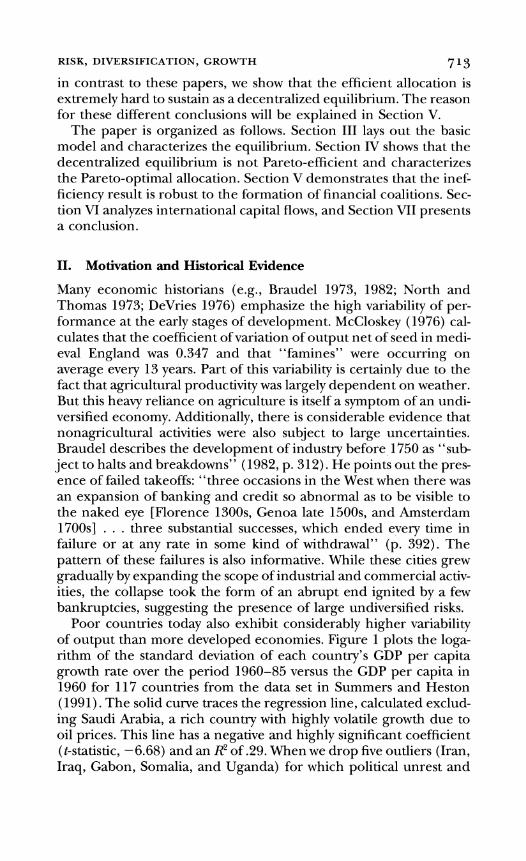
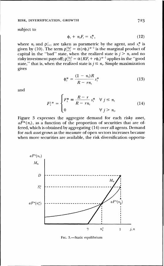
Figure 3 expresses the aggregate demand for each risky asset, aF*(n,) ,as a function of the proportion of securities that are offered, which is obtained by aggregating (14)over all agents. Demand for each asset grows as the measure of open sectors increases because when more securities are available, the risk diversification opportu-

Y ; 1 3,n

FIG. 3.-Static equilibrium


nities improve and consumers become willing to reduce their investments in the safe asset and increase their investments in risky projects. Equations (lo),(13),and (14)completely characterize the second-stage decision rules of savers.

Let us also introduce an additional assumption, which will be discussed below.

ASSUMPTION1. R 2 (2 - y) r. The following proposition characterizes the static equilibrium

conditional on Kt. PROPOSITION1. Suppose that assumption 1 holds and let

where l7 -A(l - a)[P/ (1 + P)].Then there exists a unique equilibrium such that, in the first stage, for all h E R,,either Z;,= 0 or Z;,= (j,I), where j E [0,$ 1 ; and, for all j E [0,n:], there exists h E R,such that Z;,= (j,1). In the second stage,

and $: and Fj* are given by (13)and (14).Factor returns are given by (3)and (4).

This equilibrium is expressed as the intersection of the aggregate demand of each risky asset, aF* (n,),with the thick curve that traces minimum size requirements in figure 3.When K,> (D/T)'I*, aggre-gate savings Sf 2 D,there are sufficient funds to open all the projects, and n: = 1. In contrast, when aggregate savings S: (= as:) < D,n: (Kt)< 1. In this case, only projects in [0, are open. n: (Kt)] The intuition for why n: (K,)is the equilibrium is given by the figure. If an agent proposed to open one more sector, each agent would invest more in risky projects but not sufficiently to cover the minimum size requirement of the next project because minimum size requirements grow faster than asset demands. But for all n < n:, an agent can offer to open one more project, raise enough funds, and make some positive profit v ; thus the equilibrium must be at n:.

7 2 5 RISK, DIVERSIFICATION, GROWTH

Assumption 1 is important in ensuring uniqueness.' In figure 3, when ST < D, there is only one intersection; thus the equilibrium is unique irrespective of this assumption. However, if R < (2 - y) r and Sr rD, aF*(n,)would cross Mntwice, and there would be multiple equilibria: although the amount of savings is sufficient to open all sectors so nf = 1 is an equilibrium, there will also exist another equilibrium: each agent, expecting others to invest part of their savings in the safe asset, reduces his investment in the risky projects; therefore, there are not sufficient funds to open all risky projects. Assumption 1 rules out this possibility. In Section V, we shall show that when financial coalitions are allowed, this coordination failure equilibrium can be ruled out and assumption 1 is unnecessary. Until then, it simplifies our exposition.

D. The Dynamic Equilibmum Path

Proposition 1 characterizes the equilibrium allocation and prices for given Kt. To obtain the full stochastic equilibrium process, the equilibrium law of motion of Kt needs to be determined. From (3) , ( l o ) , ( 1 3 ) ,and ( 1 4 ) ,this stochastic process is obtained as

where nf = n*(K t ) is given by equation ( 1 5 ) .The capital stock follows a Markov process in which the level of capital next period depends on whether the economy is lucky in the current period (which happens when the risky investments pay off, with probability n:). Moreover, the probability of this event changes over time. As the economy develops, it can afford to open more sectors, and the probability of transferring a large capital stock to the next period, n:, increases. Also from ( 1 6 ) ,the expected productivity of an economy depends on its level of development and diversification. To see this, define expected "total factor productivity" (conditional on the proportion of sector open) by

o P ( n * ( K t ) )= ( 1 - n*) r ( l - n*)

R + n*R . (17 )R - rn*

'It is possible that, along the equilibrium path, an agent makes an announcement of the form Z,, = (j,4) for some j EJ,(Z*), where P, > 1;as long as another agent h' has Z,, = ( j, l ) ,no consumer will buy security jfrom h. Therefore, this announcement is equivalent to Z , = 0.To economize on notation, we ignore these announcements in the statement of proposition 1.


I II I1 : I11 ; /Iv/I

>od draws

KQSSB K KSS Kt

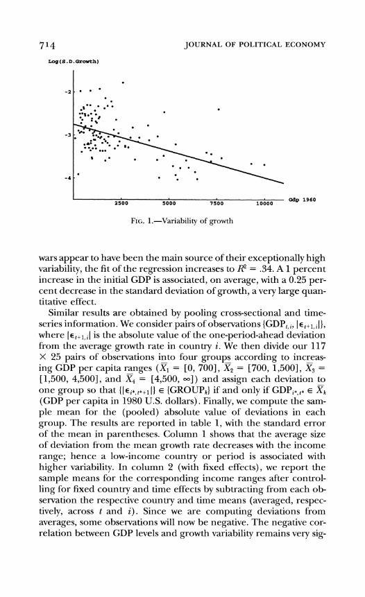
FIG. 4.-Capital accumulation

Simple differentiation establishes that as n: increases, this measure also increases.

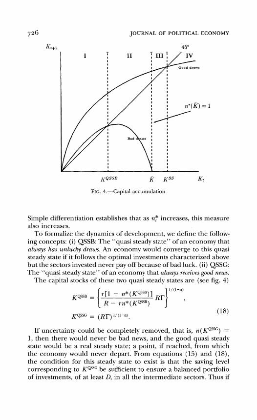
To formalize the dynamics of development, we define the following concepts: (i) QSSB: The "quasi steady state" of an economy that always has unlucky draws. An economy would converge to this quasi steady state if it follows the optimal investments characterized above but the sectors invested never pay off because of bad luck. (ii) QSSG: The "quasi steady state" of an economy that always receives good news.

The capital stocks of these two quasi steady states are (see fig. 4)

If uncertainty could be completely removed, that is, n(KQSSG) =

1, then there would never be bad news, and the good quasi steady state would be a real steady state; a point, if reached, from which the economy would never depart. From equations (15) and (18), the condition for this steady state to exist is that the saving level corresponding to KQSSG be sufficient to ensure a balanced portfolio of investments, of at least D, in all the intermediate sectors. Thus if

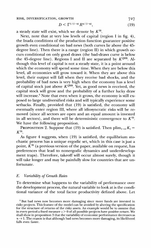
RISK, DIVERSIFICATION, GROWTH 7'7

a steady state will exist, which we denote by KSS. Next, note that at very low levels of capital (region I in fig. 4),

the Inada conditions of the production function guarantee positive growth even conditional on bad news (both curves lie above the 45- degree line). Then there is a range (region 11) in which growth occurs conditional on only good draws (the bad-draws curve is below the 45-degree line). Regions I and I1 are separated by KQSSB.Al-though this level of capital is not a steady state, it is a point around which the economy will spend some time. When they are below this level, all economies will grow toward it. When they are above this level, their output will fall when they receive bad shocks, and the probability of bad news is very high when the economy has a level of capital stock just above KQSSB.Yet, as good news is received, the capital stock will grow and the probability of a further lucky draw will in~rease .~ Note that even when it grows, the economy is still ex- posed to large undiversified risks and will typically experience some setbacks. Finally, provided that (19) is satisfied, the economy will eventually enter region 111, where all idiosyncratic risks will be removed (since all sectors are open and an equal amount is invested in all sectors), and there will be deterministic convergence to KSS. We have the following proposition.

PROPOSITION2. Suppose that (19) is satisfied. Then plim,,, Kt =

KSS. As figure 4 suggests, when (19) is satisfied, the equilibrium sto-

chastic process has a unique ergodic set, which in this case is just a point, KSS(a previous version of the paper, available on request, has preferences that lead to nonergodic dynamics and underdevelop- ment traps). Therefore, takeoff will occur almost surely, though it will take longer and may be painfully slow for countries that are unfortunate.

E. Variability of Growth Rates

To determine what happens to the variability of performance over the development process, the natural variable to look at is the conditional variance of the total factor productivity defined above. Let

But bad news now becomes more damaging since more funds are invested in risky projects. This feature of the model can be avoided by altering the specification for the structure of returns of the risky assets. An example would be to assume that in every period a fixed measure z > 0 of all possible projects have positive return. We shall show in proposition 3 that the variability of economic performance decreases as n -t 1.The reason is that although bad news becomes more damaging, its likelihood falls even faster.

728 JOURh-AL OF POLITICAL ECOXOMY

o(n*(K,)) be a random variable that takes the values [ r ( l -nT)/(R - rn?)] R and R with respective probabilities 1 - n* and n*. The mean of this random variable is given by (17). Then, taking logs, we can rewrite (16) as

A 10g(K,+~)= log T + (a - 1) log(K,) + log[o(n*(Kt)) I . (20)

It is clear from this equation that capital (and output) growth volatility, after removal of the deterministic "convergence effects" in-duced by the neoclassical technology, will be entirely determined by the stochastic component o.Define the variance of o given Kt as V,,. We want to determine how this volatility measure evolves as a function of n* (and K). Two forces have to be considered: (i) as the economy develops, more savings are invested in risky assets; and (ii) as more sectors are opened, idiosyncratic risks are better diversified.

PROPOSITION3. V, = var [o(n*, .) 1 n*] = n*(l - n*) [R(R -r) / (R - rn*)]'. (a) If y 2 R/(2R - r) , then aVn/aKt 5 0, for all Kt. (b) If y < R/(2R - r ) , then there exists K' such that n*(Kr) =

R/(2R - r) < 1 and

Io v K , ? K'

> 0 v Kt < K'.

Therefore, our model predicts that the variance of the growth rate is uniformly decreasing with the size of the accumulated capital (case a) if either y is large enough or the productivity of risky projects is sufficiently higher than that of the safe asset. Otherwise, variability exhibits an inverse U-shaped relation with respect to the capital stock (case b) and is decreasing for Kt large enough. In either case, the prediction of our model is that at the later stages of development variability is decreasing in the level of income.

F. Are the Effects Quantitatively SignzJicant ?

Our theoretical analysis so far has established that the interaction between micro indivisibilities and risk aversion leads to a slow and random path of development. An economy fluctuates in a state of low productivity before achieving full diversification and higher productivity. How important and long-lasting are these effects? A-though a more detailed analysis of this issue is left for future research, some simple calibrations would give a sense of the empirical relevance of our theory. With this purpose, we nowT use some reasonable parameter values to compute how many periods it takes for a set of simulated economies to start from KQSSR,the quasi steady state conditional on bad draws, and reach "full diversification."

RISK, DIVERSIFICATION, G R O W T H

TABLE 3

Case Mean ( T )

( 1 )

Standard Deviation ( T )

( 2 )

[ Q ~ ( l o % ) , Qr(90%)1

( 3 ) min[T]

( 4 )

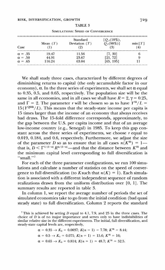
We shall study three cases, characterized by different degrees of diminishing returns to capital (the only accumulable factor in our economy), a. In the three series of experiments, we shall set a equal to 0.35, 0.5, and 0.65, respectively. The population size will be the same in all economies, and in all cases we shall have R = 2, y = 0.25, and I- = 2. The parameter r will be chosen so as to have YSS/L =

15 (YQSSB/L). This means that the steady-state income per capita is 15 times larger than the income of an economy that always receives bad draws. The 15-fold difference corresponds, approximately, to the gap between the U.S. per capita income and that of an average low-income country (e.g., Senegal) in 1985. To keep this gap con- stant across the three series of experiments, we choose r equal to 0.019, 0.184, and 0.6, respectively. Furthermore, we adjust the size of the parameter D so as to ensure that in all cases n(KSS) = 1-that is, D < rl/('-") that the distance between KSS and Ra/('-"'-and the minimum capital level corresponding to full diversification is "small. "'

For each of the three parameter configurations, we run 100 simu- lations and calculate a number of statistics on the speed of convergence to full diversification (to Ksuch that n (K) = 1).Each simula- tion is associated with a different independent sequence of random realizations drawn from the uniform distribution over [0, 11. The summary results are reported in table 3.

In column 1, we report the average number of periods the set of simulated economies take to go from the initial condition (bad quasi steady state) to full diversification. Column 2 reports the standard

'This is achieved by setting D equal to 4.1, 7.9, and 25 in the three cases. The choice of D is of no major importance and sen7es only to have indivisibilities of similar relative size in the different experiments. The initial, full diversification, and steady-state capital levels are, respectively,

a = 0.35 + KO= 0.0037; K ( n = 1) = 7.78; K S S = 8.44;

73O JOURNAL OF POLITICAL ECONOMY

deviation of this number of periods across the 100 experiments. Col- umn 3 reports the number of periods that the tenth-fastest and the tenth-slowest economies take to reach full diversification. Finally, column 4 reports how long an economy that always receives fa- vorable draws would require to complete the transition. Given the structure of the model, this is identical to the time an economy subject to no indivisibilities would take to converge to full diversification.

The results show that in all cases the effects of indivisibilities are rather long-lasting, though less so when there are strong diminishing returns to capital. W7e can assess the importance of nonconvexities on the dynamics of growth by comparing the convergence speed of the deterministic neoclassical model (col. 4) with the average convergence speed in our model (col. 1) under the same parameters. The convergence speed decreases by a factor of three when a = 0.35, by a factor of five when a = 0.5, and by a factor of 10 when a = 0.65. It is also interesting to observe that the differences between the transition length of lucky versus unlucky countries (col. 3) are very large. For instance, in all cases the tenth-most unlucky country would take more than three times as long to "industrialize" as the tenth-luckiest economy. Overall, under reasonable parameters, the effects described by this model appear very persistent and quantitatively significant.

IV. Optimal Portfolio Choice and Inefficiency

In this section we shall explain why the equilibrium of Section I11 is not Pareto-optimal and characterize the optimal portfolio decision. To focus on our main interest, we shall deal only with the issue of static efficiency. We shall therefore consider the portfolio allocation that a social planner maximizing the welfare of the current generation of savers would choose, taking the amount of savings as given.8 In contrast, in the decentralized equilibrium,J (thus n,) will also be a choice variable, F{ no longer has to equal F:', and the mar-

s With some abuse of terminology, we shall refer to this allocation as jifirst-best. Although Pareto-optimal allocations of this economy will have a portfolio decision as characterized in this section, saving decisions would in general differ. This is due in part to the overlapping generations specification. But even if we were to restrict attention to a planner maximizing only the welfare of the current generation, the saving rate would be different. First, the planner would realize that by saving more she could open more projects. Second, she would also recognize that by saving less she would increase the rate of return on capital, p,+,, and, therefore, the old-age consumption of the current generation.

RISK, DIVERSIFICATION, GROWTH 7 3 l

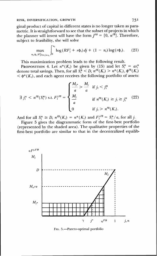
ginal product of capital in different states is no longer taken as parametric. It is straightforward to see that the subset of projects in which the planner will invest will have the form JFB = [0, nFB]. Therefore, subject to feasibility, she will solve

maa 6.'log(RF{ + re,)dj + (1 - n,) log(?-@,). (21) ~ t ~ ~ t ~ i ~ { l o ~ ~ s n ,

This maximization problem leads to the following result. PROPOSITION4. Let n*(K,) be given by (15) and let SF = as?

denote total savings. Then, for all Sf <D, nFB(K,)> @(Kt) , eFB(K,) < @*(Kt),and each agent receives the following portfolio of assets:

And for all SF 2 D, nFB(K,)= n*(K,) and FjFB = S,Y'/a, for all j. Figure 5 gives the diagrammatic form of the first-best portfolio

(represented by the shaded area). The qualitative properties of the first-best portfolio are similar to that in the decentralized equilib-

7 j* n F B 1 j , n

FIG.5.-Pareto-optimal portfolio

mailto:log(?-@,)


rium. The dynamics of the economy are still characterized by three stages: primitive accumulation, takeoff, and steady growth. But progress is faster on average because a larger share of savings is invested in high-productivity risky projects. The transition equation looks considerably more complicated than (16) because the total return is different in each state.

The reason for the failure of the decentralized economy to reach the first-best allocation is a pecuniav externality due to missing markets. As an additional sector opens, all existing projects become more attractive relative to the safe asset because the amount of undiversified risks they carry is reduced, and as a result, risk-averse agents are more willing to buy the existing securities. Since each agent ig- nores his impact on others' diversification opportunities, the externality is not internalized. It is important to reiterate at this point that in this model markets are not assumed to be missing; instead, the range of open markets is endogenously determined in equilibrium.

The pecuniary externality is not internalized in our economy because project level indivisibilities make the aggregate production set nonconvex (this is also the reason why lotteries would not be useful in this setting). As a result, a full Arrow-Debreu equilibrium does not exist. A full Arrow-Debreu equilibrium is defined as a price map- ping PA: [O,l] -+W that assigns a price to each commodity (project) +

in each time period such that, for all j E [0, 11 such that P? > 0, the excess demand for security j at time t, ed{(P:), is equal to zero, and for all j E [0, 11 such that P? = 0, ed{(Pf) 5 0. Note that this concept of equilibrium assigns a price level to all commodities irrespective of whether they are being traded or not.

The nonexistence of a full Arrow-Debreu equilibrium can be explained in terms of supply and demand. For a sector with a positive minimum size requirement, the supply is discontinuous, because if x is less than the minimum size requirement, x units of this security cannot be supplied at any price. This is the reason why a decentralized equilibrium exists only conditional on the set of open sectors. This result is related to the general equilibrium literature with endogenous commodity spaces (see Hart 1979; Makowski 1980), which, for the same reason, uses weaker versions of the Arrow- Debreu equilibrium similar to our equilibrium concept. The equilibrium concept we use captures all the salient features of a competitive situation. In particular, in our equilibrium, all agents are price takers, there is unfettered competition at all stages, and all the gains from trade that can be exploited via a decentralized trading proce- dure are exploited. The main distinction is that the requirement that markets that are closed must have ed{(P,) 5 O at Pi = O is re-

RISK, DIVERSIFICATION, GROWTH '733

placed by the condition that the number of open markets is determined by a forward-looking and fully rational free-entry c~nd i t i on .~

To conclude, also note that government policy can restore efficiency by subsidizing large projects. It is interesting that this policy appears similar to the industrial policies sometimes adopted at the earlier stages of development, for instance the policy of the German government that, despite the absence of any obvious technological spillovers, subsidized large undertakings at the expense of light in- dustries (see Gerschenkron 1962, p. 15; Cameron 1972).

V. Inefficiency with Alternative Structures

A. General iVlotivation

Would the market failure in portfolio choices be overcome if some financial institution could coordinate agents' investment decisions? Imagine that rather than all agents acting in isolation and ignoring their impact on each others' decisions-which is the source of inefficiency in Section 111-funds are invested through a financial intermediary. This intermediary can collect all the savings and offer to each saver a complex security (different from a basic Arrow security) that pays R F $ ~ ~+ r $ y in each state j , where ~f~~and $7are as described in proposition 4. Holding this security would make each consumer better off compared to the equilibrium of proposition 1.Al-though from this discussion it could appear that the inefficiency we identified may not be robust to the formation of more complex financial institutions, we shall show that this is not the case. Unless some rather strong assumptions are made about the set of contracts that a financial intermediary can offer, the unique equilibrium allocation with unfettered competition among intermediaries will be identical to the one we characterized in proposition 1.

The role of financial intermediaries and coalitions in overcoming various types of trade frictions and informational imperfections has been studied by a number of authors (e.g., Townsend 1978, 1983; Boyd and Prescott 1986; Greenwood and Jovanovic 1990; Green-

'The closest equilibrium concept is that of full Walrasian equilibrium proposed by Makowski (1980). Makowski defines a full Walrasian equilibrium as a feasible competitive allocation sustained by the set of traded commodities such that "no firm sees that it can increase its profits by altering its trade decisions assuming that the set of marketed commodities other than its own will remain the same" (p. 228). Allen and Gale (1991) also obtain a similar inefficiency. In their model the possibility of short sales implies that financial innovators will not receive the full benefits of the new assets they introduce. However, in Allen and Gale's economy, even when transaction costs are infinitesimal and there are no entry barriers, not all agents are price takers. In contrast, in our model, inefficiency arises with price-taking behavior and without short sales.


wood and Smith 1993). The approach followed in this subsection closely resembles that of Townsend (1983), who also constructs a multistage game in order to model how coalitions of agents will form to internalize some of the externalities of imperfect information and to reduce the costs of trade. However, in contrast to these papers, in our economy financial coalitions will not be able to restore efficiency.

B. Coalitions as Investment Funds

In order to model endogenous formation of coalitions, we now assume that savings can be intermediated by agents who decide to act as middlemen and run an investment fund. Put differently, some agents initiate the formation of a coalition of agents that buys securities on behalf of its members. In return, participants in the financial coalition can be charged an intermediation fee, F. Projects are still run by agents. We now introduce the following three assumptions for our coalition formation game.

ASSUMPTION2. An agent cannot be part of two coalitions at the same time.

ASSUMPTION3. Coalitions at all points maximize a weighted utility of their members. In particular, a coalition cannot commit to a path of action that will be against the interests of its members in the continuation game.

ASSUMPTION4. Coalitions cannot exclude other agents (or coalitions) from investing in a particular project.

Assumption 2 is introduced to simplify the objective function of coalitions (see Townsend [I9831 for more discussion of the case in which agents belong to multiple coalitions). As discussed below, our results hold when this assumption is relaxed. The most important assumption for our purposes is assumption 3. We view this as a very natural restriction along the lines of subgame perfection, and its importance will be discussed further below. Assumption 4 is also mainly expositional. We shall see that as long as assumption 3 holds, coalitions would never want to exclude others, and thus this assumption is imposed only to simplify the exposition.

Formally, the game played among the savers at time t now has three stages. To simplify the notation, we shall suppress time subscripts. In the first stage, each agent h E R can announce that he is willing to act as an intermediary for a specified set of agents Z h (where E h E Y, the set of all subsets of R,and we define y as the Lebesque measure over Y) . In general, only a subset of agents belonging to Ehwill accept the offer of the intermediary. Let =;I G E h denote this subset of agents. Note that because of assumption 2, in


equilibrium, Y will be partitioned into disjoint coalitions. The intermediary h will invest the savings he collects in the shares of both risky and safe projects so as to maximize the total utility of the agents belonging to E;I. A first-stage strategy for agent h is an announcement zL" = (Vh, Eh) E fRf X Y. If agent h announces that he will not act as an intermediary, then Zf' = 0.Among the possible non- null announcements, there is autarky; that is, 2:' = (0, {h}),which means that hwill intermediate only (at most) his own savings. Finally, we denote the set of first-stage announcements of all agents by 2"): R -+ R' x Y.

In the second stage, each agent h E R can announce his plan to run at most one project and sell the corresponding basic Arrow security; that is, h announces a pair ( j, $,J,as in the game discussed in Section 111. But now, securities are sold to financial intermediaries rather than directly to agents. Formally, the second-stage announcement for agent his ZL2' = ( j , <,,) E [0, 11 X R+, and 2"):R -+ [0, 11 X fRf is the set of all second-period announcements. We shall also denote the set of minimum security prices announced in the second stage of the game by P = {Pl},,, (see Sec. 111).

In the third stage, each agent takes the set of prior announcements, 2'') and Z('), as given and chooses which coalition to join. Or, equivalently, Zf' is h's choice of an intermediary from Mh[Z")] = {iE R I 2:') = (V,,E,), h E EL},the set of coalitions that announced his name. Note that although the set M,[Z")] could be empty, this will never be the case in equilibrium, since any agent can costlessly make the autarky announcement in the first stage. Finally, after all agents announce which coalition-intermediaiy they will belong to, each intermediary makes the optimal investment decision. We still use the notation @,and Fi to denote the investment of an agent (through a coalition) in the safe and risky assets. More precisely, if a coalition E invests F', in project j, then Fi will be the share of agent h in this coalition times F',.

DEFINITION2. A perfect equilibrium is a set of announcements Z* = (Z(')*, Z(')*, Z(3)*) at each stage of the game; a price function P*(Z*) for all basic Arrow securities; a saving decision s; (Z*); induced holdings of the safe asset @; (Z*) and securities Fi* (Z*) for all agents; and factor payments W* and p* such that, given the announcements of the previous stage(s) and the announcements of all other agents in the current stage, every agent chooses 2;) that maximizes his utility as given by (5) and factor returns are determined by (3) and (4).

Note that the definition of equilibrium used so far was also subgame perfect. Here we emphasize perfection in order to reiterate the importance of assumption 3 in our analysis.


C. Equilihum with Coalitions

The first observation is that free entry will drive profits (commissions) to zero in both the first and second stages. This is established by the following lemma (proof omitted).

LEMMA2. In equilibrium, (i) PJ*(Z*) = 1, for all j , and (ii) V h = 0, for all h E R.

With this remark, it is now possible to establish the following proposition.

PROPOSITION5. The set of (perfect) equilibria is nonempty, and all allocations in this set have the following characteristics: (1) For all h E R, Mh # 0 (all agents are included in some coalition). (2) Let n: be defined as in (15). Then, for all h E R, either zL2'* = 0 or Zi2'* = ( j , I ) , where j E [0, $1. And, for all j E [0, nf] , there exists h E R such that zL2'* = (j,1). (3) In the third stage, all coalitions Ei # 0 will choose a portfolio that induces @: and Fj* = FF:: as given by equations (13) and (14).

The most important feature of this set of equilibria is that they all give rise to the same allocation as the competitive equilibrium of Section 111. Note in particular that the$&-best allocation is not an equilihum of the game with intermediaries, whereas one of the equilibria has Eh = {h} for all h; that is, all agents choose autarky, which is identical to the situation without intermediaries (i.e., proposition 1). First, consider an allocation in which there is only one active intermediary, a "grand coalition" of all savers (i.e., 2:; = (0, a) for one agent h{ and zL" = 0 for all h # h"), which will invest in the optimal portfolio in the third stage of the game. If all agents agree to take part in this grand coalition, then the resulting allocation would be Pareto-optimal. However, an agent h' # hgcan do better by announcing Zi!' = (0, {h'}) and holding a balanced portfolio of all the available assets since in the second stage he cannot be excluded from investing his savings in the traded securities, JFB.Be-cause only one agent has deviated, what the grand coalition can achieve has not changed. Therefore, maximizing the utility of its remaining members, R\h', the grand coalition will choose to open JFB,and its members will have utility UFB.On the other hand, h' could hold a balanced portfolio of all j E JFBand would get utility Uh,> UFB.Therefore, all agents would prefer to deviate, and the first-best portfolio cannot be sustained as an equilibrium. The intuition for why the grand coalition is not successful is that it is trying to induce its members to hold a portfolio that cross-subsidizes large projects by investing more in them than in small projects. But, from lemma 1, when each agent takes the set of traded securities as given, he prefers to hold a balanced portfolio; thus any agent h' can pee-ride by not


becoming part of this coalition and investing his funds individually in the form of a balancedportfolio. This intuition also reveals why coalitions could deal with market failures much more effectively in the previous analyses. In the studies referenced above (e.g., Townsend 1983; Boyd and Prescott 1986), there was no issue of free-riding or cross-subsidization; therefore, all agents wanted to belong to some coalition to avoid informational problems or economize on transaction costs. In contrast, here they can free-ride by not taking part in the coalition that invests in large projects.

Next, consider the allocation in which every agent intermediates his own funds and invests them in a balanced portfolio as in proposition 1.A coalition, Eh', of a positive measure of agents could improve on this allocation by carrying out some degree of cross-subsidization, that is, by holding an unbalanced portfolio. However, ifwe start from complete autarky and h' announces Zi!' = (vh',Eh'),not to join E,, is a dominant strategy for all h" E Eh'. Intuitively, given any third-stage choice of all other agents belonging to Eh', h" would find it optimal to let other members do the cross-subsidization and just free-ride on their actions by choosing a balanced portfolio. Note that autarky (each agent intermediating his own funds) is not the unique equilibrium. Other equilibria also exist, but they all lead to exactly the same allocation as in proposition 1.

It is worth noting that if assumption 2 were relaxed, the results would not change. Irrespective of whether they have to belong to only one coalition or not, given assumptions 3 and 4, agents would always free-ride by not joining any coalition that holds an unbalanced portfolio. Thus first-best would never be sustained and autarky would remain an equilibrium.

There is, however, one difference between the equilibrium of proposition 1 and the one here. In proposition I , without assumption 1,multiple equilibria were possible for SF 2 D. In one equilibrium, all risky projects would be open and all the idiosyncratic risks would be diversified (n, = 1 and I$, = 0); in another, n, would be less than one (and I$, > 0 ) . It is straightforward to see that in this case, the equilibrium with all sectors open is Pareto-superior. Now if, instead of the decentralized equilibrium concept of definition 1, we used the coalitional approach of this section, the equilibrium with $, > 0 would disappear because the coordination failure that led to this equilibrium would be prevented by the entry of an intermediary proposing the grand coalition and offering a riskless portfolio with return R. Since in this case the grand coalition also holds a balanced portfolio, there is no scope for free-riding and all agents would agree to take part. Therefore, although the formation of coalitions does not enable cross-subsidization to be sustained in equilib-

73$ JOURNAL OF POLITICAL ECONOMY

rium, it can avoid other sources of inefficiency such as coordination failures.

D. Robustness under Alternative Assumptions

This discussion also suggests that there are some alternative assumptions under which the first-best portfolio could be implemented as a decentralized equilibrium.

First, it is easy to see that if a coalition can commit to a non-subgame perfect path of action, then the first-best can be implemented by a grand coalition of all savers. For instance, imagine that the grand coalition can commit to the following course of action: If all agents join (i.e., Z,, = R), then we invest in JFB. If even only one agent does not join (i.e., EGCf R), then $, = s,; that is, all savings are invested in the safe asset. In this case, agent h', who contemplates free-riding, will realize that by opting out of the grand coalition, he would not get a balanced portfolio of [0, n y ] but one that has a low rate of return that is naturally dominated by taking part in the grand coalition. Therefore, this type of commitment can implement the first-best. However, this is a commitment to take a course of action that would hurt all the members of the coalition. If, after h"s devia-tion, the members had the option to revise their plans, they would always prefer to do so and invest in an unbalanced portfolio of nFB assets. Consequently, we view such a commitment as extremely strong and noncredible.

Second, consider relaxing assumption 4. In particular, suppose that coalitions can buy up projects and exclude all other intermediaries from investing in the projects they control. Then the grand coalition can form and make potential members a take-it-or-leave-it offer of the following form: Either you invest all your savings in this coalition or you will be excluded. This arrangement would sustain the first-best portfolio as an equilibrium. However, such exclusion would again run into credibility problems. To see why, consider a deviation from the grand coalition such that agent h' offers to form a coalition for a set of agents Eh' with 0 < p(Zh')< l12. After this deviation, the new coalition Eh' offers to invest part of its funds in the high-minimum size projects controlled by R\Zh'. At this stage, as in the previous case discussed above, it is in the interest of all the members of R\Zv to accept these investments, because otherwise they will have to run many fewer projects and bear a lot more risk. If these investments by Ehfare accepted, then the members of =,, are better off than they would have been in the grand coalition. Therefore, again, unless R can commit to a path of behavior that does not maximize its members' utility in the continuation game, there is a profitable


deviation that breaks the first-best allocation. This argument shows that, as long as assumption 3 holds, assumption 4 is not important in deriving the results of this section.

As well as raising credibility/commitment issues we have just discussed, both cases sketched above have the unrealistic implication that only one large intermediary would be active in equilibrium. With more realistic intermediation technologies (e.g., increasing average operational costs for the intermediaries), not even these strong commitments would be sufficient to implement the first-best allocation. Therefore, this section establishes that the cross-subsidization of large projects that is required for an efficient allocation is extremely hard to achieve even when coalitions and intermediaries are allowed to form freely.

VI. International Capital Flows

In this section, we extend our model to a two-country world. Since capital shortages play a crucial role, it is important to understand whether a world of many countries behaves as a single economy or whether there would be more subtle interactions between these countries. The results will depend on the extent of capital mobility and trade. There are many different ways of modeling the interactions of two countries in this setting, and we choose the following: (1)The final good is tradable. This has two implications. First, there is full capital (savings) mobility in the sense that agents can invest their savings in the assets offered in any country.1° Second, final output produced in country i can be consumed in country i'. (2) Inter-mediate goods cannot be traded or transported from one country to another. Thus if intermediate good j is produced in country i, it has to be used in the final-good sector of country i.

Also, both countries face identical technologies and uncertainty as described in Section 111; in particular, if the (world) state of nature is j, then only sectors jl and j2are productive, where j, is sector j in country i. As an example, imagine the case in which it is not known whether railways are a good investment; if they are, then they will have high returns in both countries. These assumptions imply that

'OTo simplify the terminology, throughout the paper we referred to the total amount of intermediate goods plus the output of the safe technology as "capital." However, in the current context, this terminology could be misleading. We therefore depart from this terminology slightly and use capital mobility to refer to the case in which savings can be freely invested in the assets of the other country and use the term no trade i n intermediate goods to stand for a situation in which the output of the sector that transforms savings into capital goods (through both risky and safe technologies) in country i can be used only by final-good firms located in country i .

'74O JOURNAL OF POLITICAL ECONOMY

there are two forces to be taken into account when comparing the profitability of investments in two different countries: risk diverszJica- tion and dz;ffential pricesfor intermediate goods. To see how these two forces work, consider two closed economies such that country 1 has a larger stock of savings than country 2. According to proposition 1,country 1 has both more open sectors-that is, there will be some sector j' that is open in country 1but not in country 2-and a larger amount of intermediate goods in (at least) all realizations in which one of the open projects is successful. Given the production function (2), the marginal product of investment in country 2 will be higher. Now, introduce capital mobility. Ideally, agents would have liked to invest all their savings in one country and then transfer half of the produced intermediate goods to the other, thus maximizing both diversification and productivity. But this is not possible because intermediate goods are not traded. In terms of the example suggested above, if all railway investments are in country 1and they are successful, the final-good production of country 2 will not benefit from this success. Therefore, there will be a trade-off between a force that tends to collect funds in one country (the diversification motive) and another that pushes toward more spread-out investments (the decreasing marginal product of capital). In the remainder of this section, we shall set up the maximization problem of an agent h (which will be the same problem irrespective of where the individual lives); then we shall prove that in this context a modified "balanced portfolio" condition will hold (lemma 3) . The equilibrium solution will be characterized in proposition 6. The key results of this section are that, first, the general features of equilibrium derived in the previous section will continue to hold with international capital flows, and, second, at the early stages of development, international capital flows will serve to increase the GDP of one of the countries relative to the world average (divergence) but will later contribute to faster convergence.

The definition of equilibrium is the same as in Section 111, and all agents can announce to run any of the intermediate sector firms of this world economy. Also to simplify notation, we drop time subscripts throughout this section. The total mass of agents in the world is 2a, and agents are equally distributed between the two countries. Each agent is free to invest his funds in any combination of the two safe assets and 2 X [0, 11 risky assets. It is straightforward to see that free entry implies P,T = 1, for all j, E J,, i = 1, 2; thus all traded securities will be sold at the unit price (we drop time subscripts). Also, in each country, small sectors will open before larger ones, so J, = [0, n,]. Then, without loss of any generality, we suppose that a larger (or equal) number of projects are open in country 1 (nl 2

RISK, DIVERSIFICATION, GROWTH '74'

n2). Since all agents can buy any security issued in either country, the portfolio choice that maximizes the utility of an agent h E R1 U R2 can be written as

max log[p: ( r $ ~ + RF:,,) + p',(r$,, + RF'Zh)ldjlonz $ l h , $ 2 h , i ~ : , ~ , ~ ~ : , ~

subject to the constraint

$2,+$1,+F',, 1; +j ; '~i ,dj = s:, (24)

where

I & - a)A[K(211" if hlives in country2

is the optimal saving of individual h that depends on the wage rate in the country he lives in, and K"' is the stock of capital inherited by country i.

Let us briefly explain the terms that make up (23). Recall that nl 2 n2. Then if the realized state of nature is j E ql = [0, n2], a risky investment in both countries will have a positive payoff. If j E q2 = [n2, nl], then only risky investments in country 1will have a positive payoff. Finally, if j E q3 = [n,, 11, no risky projects will be successful. Note also that when making their decisions, all agents take the price of intermediate goods (capital) p as given. However, it is important to note that in contrast to Section 111, these prices are not necessarily equalized between countries (i.e., p{ f p i ) because intermediate goods are nontradable. The next lemma parallels lemma 1 of Sec- tion 111. (The proof of this lemma and the proofs of all the other results in this section are contained in App. B, which is available from the authors on request.)

LEMMA3. (i) For all h and for all j , j' < n2, we have F:, = F]'l h =-

Flhand F',, = FL = F2,. (ii) For all h and for all j, j' E [n2, nl], we have F:, = FL = G,.


This lemma is a weaker version of lemma 1. If two projects j and j' are open in both countries, then in each country, they should receive the same amount of investment because they have the same probability of success, the same return when they are successful (i.e., p l, = p {'), and the same equilibrium price. If two projects are open only in country 1, then, with a similar reasoning, they should again receive the same level of investment. Given lemma 3, we can reduce program (23) to

max n2 log[p;"' ( rq lh + RFlh)+ p?' (rqZh+ R F d I F l h s F 7 h , G h , @ l h @2h

subject to

where plql'denotes the price of intermediate goods in country i and in the subset of states qi. For instance, pjB' = aA(r$;")"-' and pF1' = aA(r$: + RFY)"-l, where $? denotes total world investment in the safe asset issued in country 1, F;"denotes total world investment in each open sector in country 2, and so forth. By analogy, we define cp ' as the consumption of agent h in states ql. We also let Sy' = (1 - ~ ) A { [ K ) ~ ' ]" + [K)"]"} denote the stock of world savings. We can now fully characterize the equilibrium of this two-country world.

PROPOSITION6. The unique equilibrium allocation is as follows: (i) If n; < 1, then RFTh + r$$, = RFfh + r$& (* piq1'= p?' p'ql'); $Th < $fh ( jp;q3' 2 p p ' ) and G t > Frh> Fth(=+ pp' > p'91'

> pi""). (ii) If n$ < 1, then cF1' > c?' > cp' , for a11 h E R1 U R2. (iii) There exists S'" E (D, 2 0 ) such that if S" < S"',then n; < n: < 1 and $Th > 0. If S a t >S"', then n: < nf = 1 and $Th = 0. If S w > 20, then n; = nT = 1.

The first part of proposition 6 is obtained from the first-order conditions of the program (26)-(27). The general form of the resulting aggregate equilibrium investments is plotted in figure 6 (where G*" = jQ,,Q,Gtdh, etc.). The first equality of part i ensures that the marginal return of investment is the same in both countries for the subset of states [0, n t ] . If this were not the case, an agent could increase his return in those states by just reshuffling Flhand FZh. TO see why $Th < $fh, note that the insurance role of the safe asset is less important in country 1 than in country 2. Finally, in states j E [ n t , n;], the higher minimum size requirement forces G t > FTh.

Part ii of proposition 6 reveals the most salient features of this

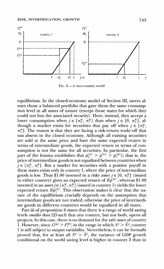
RISK, DIVERSIFICATION, GROWTH

F:" Fz'"

country 1 .'43 country 2

FIG. 6.-A hvo-country world

equilibrium. In the closed-economy model of Section 111, savers always chose a balanced portfolio that gave them the same consumption level in all states of nature (except those states for which they could not buy the associated security). Here, instead, they accept a lower consumption when j E [n; , n r ] than when j E [0, n t ] , al-though a market exists for securities that pay off when j E [ n f , n ? ] .The reason is that they are facing a risk-return trade-off that was absent in the closed economy. Although all existing securities are sold at the same price and have the same expected return in terms of intermediate goods, the expected return in terms of consumption is not the same for all securities. In particular, the first part of the lemma establishes that p?' > p"" > pjY"); that is, the price of intermediate goods is not equalized between countries when j E [n:, n r ] . But a market for securities with a positive payoff in these states exists only in country 1, where the price of intermediate goods is low. Thus $1.00 invested in a risky asset j E [O,n t ] (issued in either country) gives an expected return of ~ p ' ~ l ' ,whereas $1.00 invested in an asset j~ [ n f , n r ] (issued in country 1) yields the lower expected return Rpjq2'. This observation makes it clear that the nature of the equilibrium crucially depends on the assumption that intermediate goods are not traded; otherwise the price of intermediate goods in different countries would be equalized in all states.

Part iii of proposition 6 states that there is a range of world saving levels smaller than 2 0 such that one country, but not both, opens all projects. In this case, there is no demand for the safe asset of country 1 . However, since G*" >F?", in the range in which S" > S",country 1 is still subject to output variability. Nevertheless, it can be formally proved that, for at least all S" > S", the variance of GDP growth conditional on the world saving level is higher in country 2 than in


country 1 (see App. B). So, the prediction that growth is more volatile in poorer countries carries over to this two-country extension. Finally, as the stock of savings reaches 20, all projects will open, all risks will be diversified, and the allocation of resources will be exactly the same in the two countries.

The dynamic implications of international capital flows are interesting and can be seen by considering the following example. Sup- pose that the world consists of two closed economies with equal capital stock, and the total stock of savings is larger than P b u t less than 20, so that without capital flows both countries have n* < 1. Then consider the introduction of international capital mobility. First, funds will flow from country 2 to country 1,and country 1 will open all the sectors. Now, if a state j E [O, n f ] occurs, the realized income and next generation's wages will be the same in the two countries. However, if j E [n:, 11, GDP in country 1 will be higher than in country 2." Therefore, international capital flows lead to divergence between the two countries. Nevertheless, after some time, as the world economy becomes sufficiently rich, the direction of net capital flows will be reversed, and this time the relative GDP of country 2 will increase. In particular, as S"'+20, the two countries will converge to the same level of GDP. Therefore, the typical pattern we predict is divergence first with capital flowing to the richer country, and then a reversal of capital flows and convergence (at a faster rate than if the two economies were closed). This is similar to the pattern that Neal (1990) documents over the eighteenth and nineteenth centuries in Western Europe as the direction of capital flows between Amsterdam and London reversed.

Overall, this section shows that, conditional on no trade in intermediate goods, the two-country world does not behave like a large closed economy, and the introduction of international capital flows both enriches our framework and yields additional implications that appear consistent with historical developments. We believe that this case has empirical relevance since many intermediate goods appear to be nontraded (e.g., railways). However, if we allowed trade in intermediate goods as well as full mobility of savings, the world economy would behave like a large closed economy.

l 1 Note that there is an important difference behveen GDP and gross national product in this model. Since both countries are assumed to have the same level of sallngs, even if country 1 has a higher GDP, GNP (and consumption) will be equal because agents are choosing identical portfolios. However, this is true only for the first generation, because, later, wages will differ in the two countries. Also, the implications about the randomness of growth depend on whether we use GDP or GNP. In particular, the variability of GNP will be the same for both countries, though it will also decrease over time. With more realistic preferences (e.g., bequests or longer horizons), it is easy to generate more GNP variability in poor countries.

RISK, DIVERSIFICATION, GROWTH

VII. Conclusion

We argued in this paper that a model of development linking capital accumulation to the extent of market incompleteness yields a number of new insights. In a growth model with micro-level nonconvexities and uncertainty, we showed that the process of development goes hand in hand with better diversification opportunities and more productive use of funds. We demonstrated how primitive accumulation is followed by takeoff and financial deepening, how failed takeoffs can occur, how variability of growth decreases with development, and how productivity endogenously increases as the diversification opportunities improve. We also established that although all agents are price takers and there are no technological externalities, the process of financial development will be inefficient because of a pecuniary externality that we identie. This is not only a new source of inefficiency, but also one that, in contrast to many others that previous literature studied, cannot be internalized even when cost- less formation of complex intermediaries is allowed.

Appendix A

To simpli* the notation in the proofs, we shall drop the time subscripts when this will cause no confusion.

Proof of Lemma 1

i) We have P, = 1 for all ;l E J(Z*). Now let A be the Lagrangean of (5) subject to (6)-(9). Then it is straightforward that dA/dFI = dA/dFI', for a11;l,;lfEJ(Z*); thus for all j, j' E J(Z*), FI = Fl' = F.

ii) First, observe that (a) s = [P/(1 + P)]w (from [ lo] ) ; (b) P, = 1 for all j E J(Z*); and (c) for all ;l,;lfE J(Zm),FI = Fi' = F (from part i). Let I] E (0, 1) be an index denoting whether sector j is open or not. Then any competitive equilibrium given the prices (as in part b) and the demand functions of individuals (as in parts a and c) must be a solution to the following second-best planning problem:

max log [pl(rq + RFIl) d;l (-41 4 ~ ~ ' l i l < , S l

subject to

where pj's are taken as given. In other words, given prices and demand


functions, the equilibrium must maximize the welfare of the representative consumer.

Let Y4= [p/ (1 + p)]w - $. Conditional on $, the problem is equivalent to choosing F and {I-'),,,,,to maximize (Al)subject to the constraints F jh I1= Y4and F 2 MI",_.

Next note that irrespective of {I]), all feasible portfolios have given Yo, exactly the same return, but the variability is a decreasing function of I]. Since agents are risk-averse, the optimum must therefore maximize j; I] subject to feasibility. This is achieved by setting F = and I-'= 1 for all j5 j,,($), and j,, ($) is such that j,,($) = min [Yo/M 11.This argument applies for any $; thus, a fortiori, it applies for the $ that is the solution to the program, that is, $ = $*. Let n* = j,,($*). Then J(Z*)= [0, n*]. This completes the proof of the lemma. Q.E.D.

Proof of Proposition 1

The terms $* and F* are the unique solutions to (1 1) -(1 2), and s* is given from (10)and (3).To prove that n*(K)as defined by (15)is the unique equilibrium, we shall use the aggregate demand function aF*(n)as drawn in figure 3.We shall first show that, when S* 5 D, aFm(n)= M,for a unique value of n E [0, 11, and when S* > D, aF*(n)> M, for all n E [0, 11.

Observe that the solutions to aF*(n)= M,,can be given as the roots of a quadratic:

where we denote the smaller root by n(,). When S*<D, inspection of (A3) shows that 0 < n,,,< 1< n(,,,and both roots are real. In contrast, when S* > D and assumption 1 is satisfied, it is straightforward to see that neither n,,,nor n(2)belongs to the real interval [0, 11. Since aF*(O)= [(R-r)/R]S*> M,= 0 and both aFm(n)and M, are continuous in n in the range [0, 11, aF* (n) > M,for all n E [0, 11.

To show that, when S* 5 D, n* = n(,,(as in eq. [15])is the unique equilibrium, recall that, from lemma 1, J(Z*) = [0,El.Next suppose that -n < nT as given by (15).Then there exists h with 2 , = 0 who can deviate to Zh= ( 5+ E, 1 + E);and for E sufficiently small, IF* - Fn+'I< 6,, which implies that Z his feasible and uh> 0,a contradiction. The same argument can be used to establish that when S* > D, n< 1cannot be an equilibrium; thus n* = 1 is the unique equilibrium. Next, going back to the case in which S* < D, suppose that J(Zm)= [0,ri] such that ri > n*.Note that

RISK, DIVERSIFICATION, GROWTH 747

W e n assumption 1 holds, aaF* ( l ) / a n = r/ ( R - r ) < D/ ( 1 - y); thus aaF* ( n ) / a n <D/ (1 - y) for all n E [0 , 11 .Thus at the point of intersection n* (fig. 3 ) , a F m ( n )is less steep than M,. Then aF*(li) < M,; hence this allocation is not feasible. Therefore, J ( Z * ) = [0 , n*] is the unique equilibrium. It is then straightforward, from free entry at stage 1, that, for all j E [0, n*] , there exists h such that Z , = ( j , 1 ) . Q.E.D.


Let K = ( D / T ) l / a .Then (15) implies that, for all Kt 2 n*(K,) = 1. Next, (19) implies that K < KSS= ( R T ) ' / ( l - u ' ;thus if Kt 5 K, then Kt,, =

RTKP, and Kt converges deterministicall) to KSS.Equations (15) and (16) imply that the set [ O , El has no absorbing subset (except for the point zero) since, for all K, > 0, K,,, = RTK? > K, with probability n * ( K t )> 0 (the economy grows conditional on good news). Therefore, we need only to show that from any point in (0 , K ) there is a positive probability that Kwill be reached. We alreadyobserved that, conditional on good news,

= RTK? and Kt + KSS> K. Hence, for all KO> 0 , there exists a sequence of N ( K o )good draws such that K,,(,,, > and this sequence occurs with positive probability. Therefore, plim,,, Kt = KSS.Q.E.D.


The variance of o(n* ( K ) ) is

V, = ( 1 - n*) r ( l - n * ) R

- o e ( n * ( K ) ) + n * [ R- o e ( n * ( K ) ) I S ,R - rn* I'

where o e ( n * ( K ) )is defined by (17) in the text. Simple algebra establishes that V, = n*( l - n*) [ R ( R - r )/ ( R- rn*)]

and sign (aV,,/an*) = sign ( R- 2n*R + rn*) . Thus if n* > R / ( 2 R - r ) , then aV,/an* < 0. We also know from (15) that n* > y. Therefore, if y > R / ( 2 R - r ), then V, is decreasing in n* everywhere. Otherwise, it will be nonmonotonic (inverse U-shaped with n* = R / [ 2 R- r] maximizing V,). Since (15)implies anm/dK? 0 for all K, the rest of the proof follows. Q.E.D.


We shall first prove that no allocation with a balanced portfolio can be optimal and then show that the optimal allocation will look as in figure 5.

The expected utility from second-period consumption for the representative agent, when individual savings are equal to s* and J = [0, n ] , can be written as


Taking partial derivatives of U ( . )with respect to n and {Fi)and evaluating them at the decentralized equilibrium, n = n* and F-'= F*, we obtain

and

iF*)' '*) = log[RF* + r(s* - n*F*)] - log [l(s* - n*F*)] an

(A71

+ F* + r(s* - ?z*F*) + RF*(1 - n*)

[RF* + r(s* - n*F*)] (s* - n*F*) > 0.

Now let us reduce F-'for j 5 y below F* and increase n (such that ydF = F*dn). From (A4) and (A5), this will increase C'(.) . Therefore, the decentralized equilibrium is not Pareto-optimal. By evaluating dU/dn and dC'/aF at any Z 5 S*/F*(Z) and applying the same argument, we can establish that no feasible allocation with a balanced portfolio of risky assets can be a Pareto optimum when n < 1. Moreover, this argument also establishes that the planner would open more sectors than the decentralized equilibrium; thus nFB(K) > n*(K) whenever n*(K) < 1.

To characterize the first-best, let us construct the Lagrangean

A(n, lFIJ,@. h, {pi))= ionl o g ( R ~ l+ r$)dj + (1 - n) log(@) (A8)

The first-order condition with respect to F{is

Now, if two sectors j', j" E [O, n] do not have a binding minimum size requirement, then optimality requires that pi' = p-'"= O and (by eq. [A9]) F J ' , ~ ~F I " . ~ ~ .For the rest of the sectors, pl > 0 and FJ,"= liZl,/a. Next, we = prove the following three claims: (i) j > j' and p-" > O * p-' > 0, (ii) j < j' and p-'' = 0 3 p i = 0, and (iii) pi' > p-' F I ' , ~ ~ Suppose= 0 > that claim i were not true, so that p ~ ' > 0 and pi = 0. It must then be the case that aF1 > Mi > aF" = Mi,. But then it would be feasible for the planner to give each agent more insurance and the same expected return by simply reducing FI and increasing Fl' by the same amount, and this portfolio could not be optimal So claim i must be true. A similar argument can be applied to prove claims ii and iii. These three facts imply that we can define n~~= maxi j E [0, 11 s.t. F-',"'> O), where from the first part of this proof

we know that n* < nFB5 1. Then there exists j* E [0, nFB] such that, for all j < j*, Fl.pB = Ml\/a (the minimum size requirement is not binding), whereas for all j E [j*, nFB] ,F I , ~ ~= Ml/a (the minimum size requirement is binding).


For expression (22) in proposition 4 (and the allocation described by fig. 5 ) to follow, we have to show only that 0 < j* < nFB (with strict inequali- ties). Assume that j* = n"'. Then agents would be holding a balanced portfolio, which was shown above never to be a Pareto optimum. Thus j* < nFn. Assume j* = 0. This would be equivalent to not opening sectors with no minimum size requirement, and it is straightforward to see that the planner could reduce the risk borne by the agents by increasing the measure of the set JF! So j* > 0. Finally, from nFn > n* and the first-order conditions, it easily follows that (IFn < (I*. Q.E.D.


We shall first establish that all equilibrium allocations must satisfy parts 1- 3; then we shall show that the set of equilibrium allocations is nonempty.

Part 1 is straightforward, since an agent h who has Mh = 0 can always choose Z;' = (0, (h}) (autarky). Next, consider part 3. Define li,(Z%, :z) as the utility of agent h when he joins coalition E: and J(Z'2') = [O, n]. Sup- pose that there is an equilibrium in which there exists Et with p (E,) > 0 holding an unbalanced portfolio. Consider an agent h' E Zi. By lemma 1, given n, h' maximizes his utility by holding a balanced portfolio [0, n]. Since by assumption 4 there is no exclusion from the open sectors, h' can choose autarky and hold a balanced portfolio of all the open sectors. By assumption 3, after h' leaves, Z: would stiil invest in the same portfolio (or if the set of agents who did not join had positive measure E, the coalition would invest in a portfolio that would be only a small distance away from the previous choice, and exactly the same argument would apply with E

small enough). Therefore, by leaving, agent h' would receive C;; (h', n) > Uh,(Z;, n). Then, in the first stage, Z:!' = (0, (h'}) and Zi?' = (h'} is a benefi- cial deviation for all h'. Therefore, there can be no equilibrium in which the set of announcements induces an agent to hold an unbalanced portfolio. Next, lemma 2 implies that second-stage announcements will induce P(Z*) = 1 and that there can be no positive commissions. This result com- bined with a balanced portfolio for all agents immediately implies that J(Z*) = [0, n*], where n* is given by (15) and (I* and F*are given by (13) and (14). Therefore, all equilibria have to be as described in proposition 5.

Next, to prove that the set of equilibrium allocations is nonempty, it is sufficient to show that the "autarky" allocation in which Zj:) = (0, { h } ) ,for all h E R, together with parts 1-3 is in the equilibrium set. Suppose that z;) = (0, (h}), for all h E R, and that in the second stage, for all j n*(K), there exists h': Zh, = (0,j) and all agents choose a balanced portfolio over [0, n*(K)] as given by (13) and (14) in the third stage. It is clear that, given the announcements of the first stage, we are in the same situation as in proposition 1; thus ~ f 'and Zy' as described are optimal for all h. There- fore, we need only to show that there is no profitable first-stage deviation. Suppose that h' deviates to Z$' = (E, E,,), where E > 0 but can be arbitrarily small. Consider first p (Zv) = 0; then the optimal policy for this coalition in the third stage is to hold a balanced portfolio. Thus for all E > 0, the best response of all h is not to join this coalition since they would hold

7 5 O JOURNAL OF POLITICAL ECONOMY

exactly the same portfolio in autarky and would save the intermediation cost E. Now consider p(3,r) > 0. Then either this coalition will still hold a balanced portfolio, in which case the same argument applies, or it will hold an unbalanced portfolio over some set J' = [0, n'] with n' > n * ( K ) . But then by the argument we used above, each h will prefer not to join this coalition and hold a balanced portfolio over [0, n'] in autarky. Therefore, autarky (with the allocation characterized in proposition 1) is in the equilibrium set. Q.E.D.

References

Allen, Franklin, and Gale, Douglas. "Optimal Security Design. " Rev. Finan-cial Studies 1, no. 3 (1988): 230-63.

. "Arbitrage, Short Sales, and Financial Innovation." Econometrics 59 (July 1991): 1041-68.

Atje, Raymond, and Jovanovic, Boyan. "Stock Markets and Development." Europran Econ. Rev. 37 (April 1993): 632-40.

Azariadis, Costas, and Drazen, Allan. "Threshold Externalities in Economic Development." Q J E . 105 (May 1990): 501-26.

Bagehot, Walter. Lombard Street: A Description ofthe Mony Market. New York: Scribner, 1873. Reprint. Homewood, Ill.: Irwin, 1962.

Bencivenga, Valerie R., and Smith, Bruce D. "Financial Intermediation and Endogenous Growth." Rev. Econ. Studies 58 (April 1991) : 195-209.

Benhabib, Jess, and Gali, Jordi. "On Growth and Indeterminacy: Some The- ory and Evidence." Manuscript. New York: New York Univ., 1995.

Boyd, John H., and Prescott, Edward C. "Financial Intermediary-Coali- tions." J. Econ. The09 38 (April 1986): 211-32.

Braudel, Fernand. Capitalism and Matm'al Life, 1400-1800. New York: Harper and Row, 1973.

. Civilization and Capitalism, 15th-18th C e n t u ~ .Vol. 2. The Wheels of Commmce. New York: Harper and Row, 1982.

Cameron, Rondo E. "Introduction." In Banking and Economic Development: Some Lessons of his to^, edited by Rondo E. Cameron. New York: Oxford Univ. Press, 1972.

Chandler, Alfred D., Jr. The Visible Hand: The Managm'al Revolution i n Ameri- can Business. Cambridge, Mass.: Belknap Press, 1977.

DeVries, Jan. The Economy of Europe i n an Age of Crisis, 1600-1 750. Cam-bridge: Cambridge Univ. Press, 1976.

Gerschenkron, Alexander. Economic Backwardness i n Historical Perspective: A Book ofEssays. Cambridge: Cambridge Univ. Press, 1962.

Goldsmith, Raymond W. Financial Structure and Development. New Haven, Conn.: Yale Univ. Press, 1969.

Greenwood, Jeremy, and Jovanovic, Boyan. "Financial Development, Growth, and the Distribution of Income." J.P.E. 98, no. 5, pt. 1 (October 1990): 1076-1107.

Greenwood, Jeremy, and Smith, Bruce D. "Financial Markets in Develop- ment and the Development of Financial Markets." Manuscript. Roches- ter, N.Y.:Univ. Rochester; Ithaca, N.Y.: Cornell Univ., 1993.

Gurley, John G., and Shaw, Edward S. "Financial Aspects of Economic De- velopment." A.E.R. 45 (September 1955): 515-38.

RISK, DIVERSIFICATION, GROWTH 75' Hart, Oliver D. "On Shareholder Unanimity in Large Stock Market Econo-

mies." Econometrica 47 (September 1979): 1057-83. Hobsbawm, Eric J. Indust? and Empire: A n Economic Histoq of Britain since

1750. New York: Penguin, 1968. Kennedy, William P. Industrial Structure, Capital Markets, and Origins ofBritish

Economic Decline. Cambridge: Cambridge Univ. Press, 1987. King, Robert G., and Levine, Ross. "Finance and Growth: Schumpeter

Might Be Right." Q J E . 108 (August 1993): 717-37. Lucas, Robert E., Jr. "On the Mechanics of Economic Development." J.

Monetaq Econ. 22 (July 1988): 3-42. McCloskey, Donald N. "English Open Fields as Behavior towards Risk." In

Research i n Economic Histoq, vol. 1, edited by Paul Uselding. Greenwich, Conn.: JAI, 1976.

Makowski, Louis. "Perfect Competition, the Profit Criterion, and the Orga- nization of Economic Activity." J. Econ. Theoq 22 (April 1980): 222-42.

Neal, Larry. The Rise ofFinancial Capitalism: International Capital Markets i n the Age ofReason. Cambridge: Cambridge Univ. Press, 1990.

North, Douglass C., and Thomas, Robert P. The Rise of the Western World: A New Economic Histoq. Cambridge: Cambridge Univ. Press, 1973.

Persson, Karl G. Pre-industrial Economic Growth, Social Organization and Tec1~- nological Progress i n Europe. Oxford: Blackwell, 1988.

Quah, Danny. "Empirical Cross-Section Dynamics in Economic Growth." European Econ. Rev. 37 (April 1993): 426-34.

Ramey, Garey, and Ramey, Valerie A. "Cross-Country Evidence on the Link between Volatility and Growth." A.E.R. 85 (December 1995) : 1138-51.

Rosenberg, Nathan, and Birdzell, Leo E., Jr. Horu the West Grew Rich: The Economic Transformation of the Industrial World. New York: Basic Books, 1986.

Saint-Paul, Gilles. "Technological Choice, Financial Markets and Economic Development." European Econ. Rev. 36 (May 1992): 763-81.

Scherer, Frederic M. Innovation and Growth: Schumpeterian Perspectives. Cam-bridge, Mass.: MIT Press, 1984.

Summers, Alan, and Heston, Robert. "The Penn World Table (Mark 5) : An Expanded Set of International Comparisons, 1950-1988." Q.J.E.106 (May 1991): 327-68.

Tortella, Gabriel. "Spain, 1829-1874." In Banking and Economic Develop- ment: Some Lessons of Histo?, edited by Rondo E. Cameron. New York: Oxford Univ. Press, 1972.

Townsend, Robert M. "Intermediation with Costly Bilateral Exchange." Rev. Econ. Studies 45 (October 1978): 417-25.

. "Theories of Intermediated Structures." Carnegie-Rochester Conf. Ser. Public Polzq 18 (Spring 1983) : 221 -72.

. "Risk and Insurance in Village India." Econometrica 62 (May 1994): 539-91.

Wrigley, Edward A. Continuity, Chance and Change: The Character ofthe Indus- trial Revolution i n England. Cambridge: Cambridge Univ. Press, 1988.

Zilibotti, Fabrizio. "Endogenous Growth and Intermediation in an 'Archi- pelago' Economy." Econ. J. 104 (March 1994): 462-73.

You have printed the following article:

Was Prometheus Unbound by Chance? Risk, Diversification, and GrowthDaron Acemoglu; Fabrizio ZilibottiThe Journal of Political Economy, Vol. 105, No. 4. (Aug., 1997), pp. 709-751.Stable URL:


This article references the following linked citations. If you are trying to access articles from anoff-campus location, you may be required to first logon via your library web site to access JSTOR. Pleasevisit your library's website or contact a librarian to learn about options for remote access to JSTOR.

[Footnotes]

9 Arbitrage, Short Sales, and Financial InnovationFranklin Allen; Douglas GaleEconometrica, Vol. 59, No. 4. (Jul., 1991), pp. 1041-1068.Stable URL:

http://links.jstor.org/sici?sici=0012-9682%28199107%2959%3A4%3C1041%3AASSAFI%3E2.0.CO%3B2-N

References

Optimal Security DesignFranklin Allen; Douglas GaleThe Review of Financial Studies, Vol. 1, No. 3. (Autumn, 1988), pp. 229-263.Stable URL:

http://links.jstor.org/sici?sici=0893-9454%28198823%291%3A3%3C229%3AOSD%3E2.0.CO%3B2-7

Arbitrage, Short Sales, and Financial InnovationFranklin Allen; Douglas GaleEconometrica, Vol. 59, No. 4. (Jul., 1991), pp. 1041-1068.Stable URL:

http://links.jstor.org/sici?sici=0012-9682%28199107%2959%3A4%3C1041%3AASSAFI%3E2.0.CO%3B2-N

http://www.jstor.org

LINKED CITATIONS- Page 1 of 2 -

NOTE: The reference numbering from the original has been maintained in this citation list.

http://links.jstor.org/sici?sici=0022-3808%28199708%29105%3A4%3C709%3AWPUBCR%3E2.0.CO%3B2-%23&origin=JSTOR-pdf

http://links.jstor.org/sici?sici=0012-9682%28199107%2959%3A4%3C1041%3AASSAFI%3E2.0.CO%3B2-N&origin=JSTOR-pdf

http://links.jstor.org/sici?sici=0893-9454%28198823%291%3A3%3C229%3AOSD%3E2.0.CO%3B2-7&origin=JSTOR-pdf

http://links.jstor.org/sici?sici=0012-9682%28199107%2959%3A4%3C1041%3AASSAFI%3E2.0.CO%3B2-N&origin=JSTOR-pdf

Financial Intermediation and Endogenous GrowthValerie R. Bencivenga; Bruce D. SmithThe Review of Economic Studies, Vol. 58, No. 2. (Apr., 1991), pp. 195-209.Stable URL:

http://links.jstor.org/sici?sici=0034-6527%28199104%2958%3A2%3C195%3AFIAEG%3E2.0.CO%3B2-3

On Shareholder Unanimity in Large Stock Market EconomiesOliver D. HartEconometrica, Vol. 47, No. 5. (Sep., 1979), pp. 1057-1083.Stable URL:

http://links.jstor.org/sici?sici=0012-9682%28197909%2947%3A5%3C1057%3AOSUILS%3E2.0.CO%3B2-C

Intermediation with Costly Bilateral ExchangeRobert M. TownsendThe Review of Economic Studies, Vol. 45, No. 3. (Oct., 1978), pp. 417-425.Stable URL:

http://links.jstor.org/sici?sici=0034-6527%28197810%2945%3A3%3C417%3AIWCBE%3E2.0.CO%3B2-K

Risk and Insurance in Village IndiaRobert M. TownsendEconometrica, Vol. 62, No. 3. (May, 1994), pp. 539-591.Stable URL:

http://links.jstor.org/sici?sici=0012-9682%28199405%2962%3A3%3C539%3ARAIIVI%3E2.0.CO%3B2-9

Endogenous Growth and Intermediation in an `Archipelago' EconomyFabrizio ZilibottiThe Economic Journal, Vol. 104, No. 423. (Mar., 1994), pp. 462-473.Stable URL:

http://links.jstor.org/sici?sici=0013-0133%28199403%29104%3A423%3C462%3AEGAIIA%3E2.0.CO%3B2-7

http://www.jstor.org

LINKED CITATIONS- Page 2 of 2 -

NOTE: The reference numbering from the original has been maintained in this citation list.

http://links.jstor.org/sici?sici=0034-6527%28199104%2958%3A2%3C195%3AFIAEG%3E2.0.CO%3B2-3&origin=JSTOR-pdf

http://links.jstor.org/sici?sici=0012-9682%28197909%2947%3A5%3C1057%3AOSUILS%3E2.0.CO%3B2-C&origin=JSTOR-pdf

http://links.jstor.org/sici?sici=0034-6527%28197810%2945%3A3%3C417%3AIWCBE%3E2.0.CO%3B2-K&origin=JSTOR-pdf

http://links.jstor.org/sici?sici=0012-9682%28199405%2962%3A3%3C539%3ARAIIVI%3E2.0.CO%3B2-9&origin=JSTOR-pdf

http://links.jstor.org/sici?sici=0013-0133%28199403%29104%3A423%3C462%3AEGAIIA%3E2.0.CO%3B2-7&origin=JSTOR-pdf

Documents

Was Prometheus Unbound by Chance? Risk, …econdse.org/wp-content/uploads/2015/10/AcemogluZillibotiJPE97.pdf · Was Prometheus Unbound by Chance? Risk, Diversification, and Growth