Was Mr. Hewlett Right?

Mergers, Advertising and the PC Industry

Michelle Sovinsky Goeree 1

February, 2009

Abstract

In markets characterized by rapid change consumers may not know every available prod-uct. Advertising allows �rms to inform consumers about their products, but �rms�pro�t-maximizing advertising choices are not necessarily welfare maximizing. Ignoring the con-sequences of limited information and �rms� strategic incentives for providing informationin merger analysis could lead antitrust authorities to approve a merger that has negativeconsequences for welfare. I use the parameter estimates from a limited information modelin Goeree (2008) to examine the role of strategic information provision via advertising andexamine the implications for antitrust merger policy. To do so, I simulate post-mergerprice and advertising equilibria. I decompose the post-merger change in prices into changesdue to increased concentration and changes due to strategic provision of information. Theresults indicate advertising can be used to increase market power when consumers have lim-ited information, which suggests revisions to the current model used to access the impact ofmergers in antitrust cases.JEL Classi�cation: L15, D12, M37, L44, D83Keywords: merger analysis, informative advertising, discrete-choice models, product di¤er-entiation, structural estimation

1 University of Southern California, Economics Department (goeree@usc.edu). This researchhas bene�ted from comments from seminar participants at Claremont McKenna, the Federal TradeCommission, EARIE meetings (Porto), IIOC meetings (Boston), and discussions with Ulrich Do-raszelski and Michael Waterson. I am grateful to Gartner Inc. for making the data available andfor �nancial support from the University of Virginia�s Bankard Fund for Political Economy.

1 Introduction

On May 7, 2002 Hewlett-Packard (HP) Company launched the new HP with an ad titled

�We are Ready.� The new HP is a result of a merger with Compaq Computer Corporation,

the largest ever in the information technology sector. The $19 billion deal drew a lot of

media attention for a number of reasons. Investors and rival �rms were interested in its

impact on shares and pro�ts. Consumers were interested in the e¤ect on prices. Regulators

were interested in its implications for competition in an already concentrated industry.

Originally proposed in June 2001, the merger prompted a bitter battle between Hewlett

and Packard family interests and corporate executives. It was ultimately approved by a slim

majority of shareholders (only 3%). Many HP shareholders opposed the deal because they

thought the time lost in absorbing Compaq and incorporating cost synergies would distract

from winning new orders at a time when the market was slowing. Walter Hewlett, whose

father cofounded HP, initiated a court battle against HP arguing the merger would result in

lost pro�ts in the long run. As further evidence of his conjecture, Hewlett pointed to his

competitors, �We believe that HP stockholders should be concerned when competitors, like

SUN, Dell, and IBM don�t object to a transaction that is supposed to add value to HP.�

Meanwhile, the Federal Trade Commission (FTC) voted unanimously to approve the merger.

Likewise the European Commission approved it without placing any conditions on the two

companies saying, �A careful analysis of the merger. . . has shown that HP would not be in

a position to increase prices and that consumers would continue to bene�t from su¢ cient

choice and innovation.�2

Currently, antitrust authorities evaluate the impact of mergers under the assumption

that consumers know all products for sale when making their purchases. This assumption

is questionable, especially when applied to markets characterized by rapid change, such as

the personal computer (PC) industry. Advertising allows �rms to inform consumers about

their products, but �rms�pro�t-maximizing advertising choices are not necessarily welfare

maximizing and can result in increased market power at the expense of consumers. Indeed

Goeree (2002, 2008) shows that assuming full-information in a market characterized by rapid

change generates estimates of demand curves that are biased towards being too elastic. This

result is of particular importance when considering the welfare impact of mergers, the primary

interest of US antitrust authorities. Ignoring the consequences of limited information and

�rms�strategic incentives for advertising in merger analysis could lead antitrust authorities

to approve a merger that has negative consequences for welfare.

2 �HP-Compaq Merger Wins European Approval,�NewsFactor Network, Feb.1, 2002.

1

The goal of this empirical work is twofold: (1) to estimate the e¤ect on pro�ts and

consumer welfare from mergers when consumers have limited information and (2) to examine

the role of strategic information provision via advertising and the resulting implications for

antitrust policy. The methodology used to evaluate the impact of mergers is based on

previous work,3 but allows for limited information and strategic choices of advertising. I use

the estimated parameters from a structural model of limited information presented in Goeree

(2008) to simulate post-merger equilibrium price and advertising levels. I calculate the e¤ect

of mergers on the pro�ts of merging and non-merging �rms as well as the cost-synergies

necessary to o¤set losses. I decompose the post-merger change in prices and markups

into the changes due to increased concentration and the changes due to the in�uence of

information provision. The post-merger equilibrium results indicate advertising can be used

to increase market power, which suggests revisions to the current model used by antitrust

authorities to determine market power in antitrust cases.

I examine both the HP-Compaq merger and a hypothetical merger between IBM and

Dell over a period of intense growth in the PC market, 1996-1998.4 Considering a merger

between IBM and Dell is of interest for two reasons. First, IBM is the world leader in sales

of non-PC�s, while Dell�s focus is more on the sale of PC�s. As a result, cost synergies would

likely be lower than those between HP and Compaq. Secondly, and more directly related

to the topic of this research, IBM and Dell have very di¤erent ad-to-sales ratios. IBM is

a high-advertising intensity �rm (ad-to-sales ratio over 20%), while Dell is a low-intensity

�rm (ad-to-sales ratio under 3%). In contrast, HP and Compaq are thought to have more

cost synergies and are closer in their ad-sales concentration. Comparison of the outcomes

from the two very di¤erent mergers yields insight into the role that advertising plays in this

industry and how �rms use it when industry concentration increases.

Related literature forthcoming...

The remainder of the paper is organized as follows. In the next section, I discuss the

data used in estimation. In section 3, I describe the model used in the counterfactual

merger simulations. In section 4, I discuss the estimation technique and present parameter

estimates. In section 5, I discuss the impact of mergers on welfare and pro�ts, the role that

advertising plays as concentration increases, and the implications for antitrust policy. The

�nal section concludes.

3 For example, see Baker and Bresnahan, 1985; Berry and Pakes, 1993, Hausman, Leonard and Zona,1994; and Nevo, 2000.

4 While the merger is supposed, IBM and Dell entered into a $16 billion cross-licensing agreement in1999. The agreement called for broad patent cross-licensing between the two �rms and collaboration in thedevelopment of product technology.

2

2 Data

The data come from three primary sources. Product-level data are from Gartner Inc. and

consist of prices, market shares, and product characteristics of all PCs sold to home users

between 1996 and 1998. Home market sales accounts for over 30% of all PCs sold. I have

data on �ve main PC attributes: �rm (e.g. Dell), brand (e.g. Latitude LX), form factor

(e.g. desktop), CPU type (e.g. Pentium II), and CPU speed (MHz). I de�ne a model as a

�rm, brand, CPU type, CPU speed, form factor combination.5 Treating a model/quarter

as an observation, the total sample size is 2112.

Percentage DollarManufacturer Home Market Share Ad Ad to Sales Median Price

1996 1997 1998 Expend Ratio Home SectorIndustry 3.4% $2,239

Top 6 Firm 65.67 68.31 75.26 $469 9.1% $2,172

Acer 6.20 6.02 4.37 $117 5.4% $1,708Apple 6.66 5.79 9.16 $161 5.3% $1,859AST 3.08 1.53Compaq 11.89 16.29 16.43 $208 2.4% $2,070Dell 2.46 2.87 2.57 $150 2.1% $2,297Gateway 8.94 11.77 16.43 $277 5.6% $2,767Hewlett­Packard 4.02 5.52 10.05 $651 17.7% $2,203IBM 8.49 7.42 6.85 $1,189 20.1% $2,565Micron 3.26 4.05 1.68NEC 3.22Packard Bell 23.48Packard Bell ­ NEC 21.02 16.33 $327 7.2% $2,075Texas Instruments 1.40

Notes:  In 1997 three mergers occurred :Packard Bell, NEC,ZDS; Acer,Texas Instr.; Gateway, Advanced Logic Research.Ad expenditures (in $M) and ad to sales ratios are annual averages and are from LNA and include all sectors(home, business, education, government).

Average Annual

Table 1: Summary Statistics

Table 1 presents descriptive statistics for the home market sector. The top six �rms

account for over 69% (71%) of the dollar (unit) home market share on average. The major

market players did not change over the period, although there was signi�cant change in some

of their market shares. In estimation I consider the top ten �rms and �ve others (AST,

5 The data I use consist of attributes which cannot be easily altered or enhanced after purchase. Thedata allow for a very narrow model de�nition. For example, the Compaq Armada 6500 and the Armada7400 are two separate models. Both have Pentium II 300/366 processors, 64 MB standard memory, 56KB/smodem, an expansion bay for peripherals, and full-size displays and keyboards. The 7400 is lighter, althoughsomewhat thicker, and it has a larger standard hard drive, and more cache memory. In both models thehard drive and memory are expandable up to the same limit. In addition, the Apple Power MacintoshPower PC 604 180/200 desktop and deskside are two separate models. They di¤er only in their form factor.

3

AT&T / NCR, DEC, Epson, and Texas Instruments) to make full use of micro-purchase data

discussed below. The included �rms are Acer, Apple, AST, AT&T, Compaq, Dell, Epson,

Gateway, HP, IBM, Micron, NEC, Packard Bell, and Texas Instruments. Together these 15

�rms account for over 85% (83%) of the dollar (unit) home market share on average.

This study considers the period 1996-1998 when the PC industry was experiencing

tremendous growth. In 1996 Packard Bell was a 4.5 billion company and the largest PC

manufacturer in the US.6 Compaq passed Packard Bell in mid 1996 and price pressure

from Compaq and eMachines, along with poor showings in consumer satisfaction surveys,

made it di¢ cult for the company to remain pro�table. In 1997, three mergers occurred:

Packard Bell, NEC, and ZDS; Acer and Texas Instruments; and Gateway and Advanced

Logic Research.

After this period, there was a slowdown in the PC market. Demand in the home market

sector (as well as other sectors) declined. In part because there was not as much of a need

to upgrade as often since the PCs were so well made and, in part due to the slump in the

economy. Immediately after 1998, Compaq merged with DEC, which proved to be a mistake

for Compaq in that they never fully recovered their pre-merger market position. It is this

Compaq with which HP merged in 2002.

I combine the product level data with advertising data from Competitive Media Report-

ing�s LNA/ Multi-Media. These are quarterly advertising expenditures across media by

�rm with some brand level information. The expenditures are reported for ten media from

which I construct four categories: newspaper, magazine, television, and radio.7 There are

two points to make regarding the advertising data. First, they are not broken down by

sector. Hence, some of the advertising I observe is for non-PCs intended for non-home con-

sumers. Second, PC �rms may advertising their products in groups (using a combination of

product-speci�c advertising and group advertising with groups of varying sizes). For exam-

ple, in 1996 one of Compaq�s advertising campaigns involved all Presario brand computers

(of which there are 12). In Goeree (2008) I show how to deal with this issue by construct-

ing a measure of ad expenditures by product that incorporates all advertising done for the

product. I construct �e¤ective� product advertising by adding observed product-speci�c

expenditures to a weighted average of all group expenditures for that product where the

6 Packard Bell was an American radio manufacturer. The Packard Bell Company has no associationwith Hewlett Packard.

7 The Magazine medium includes Sunday magazines; TV includes network, spot, cable or syndicated TV;Radio includes network and spot radio. There are many zero observations for outdoor advertising, and so Iinclude it in the radio medium. Internet advertising was not so prevalent over this time period.

4

weights are estimated.8 As can be seen from Table 1, there is much variation in advertising

expenditures across �rms. For instance, in 1998, the majority of the industry expenditures

are by IBM, resulting in an ad-to-sales ratio of over 20 percent. While the industry average

ad-to-sales ratio is much lower, about 3%. Excluding IBM�s expenditures, the remaining

top �rms spend an average of 6.5% of their revenue on advertising. In contrast, Compaq�s

ad-to-sales ratio is only 2.4%.

Variable DescriptionMean Std. Dev.

male 0.663 0.474white 0.881 0.324age (years) 47.381 15.67630to50 (=1 if 30<age<50) 0.443 0.497education (years) 13.980 2.543married 0.564 0.496household size 2.633 1.429employed 0.695 0.460income ($) 56745.33 45246.23inclow (=1 if income<$60,000) 0.667 0.471inchigh (=1 if income>$100,000) 0.107 0.309own pc (=1 if own a PC) 0.466 0.499pcnew (=1 if PC bought in last 12 months) 0.113 0.317cable (=1 if receive cable) 0.749 0.434hours cable (per day) 3.607 2.201hours non­cable (per day) 3.003 2.105hours radio (per day) 2.554 2.244magazine (=1 if read last quarter) 0.954 0.170number magazines (read last quarter) 6.870 6.141weekend newspaper (=1 if read last quarter) 0.819 0.318weekday newspaper (=1 if read last quarter) 0.574 0.346Notes: Number of observations in survey is 39,931. Sample size is 13,400.Media exposure summary statistics are based on reports published by Simmons.

Table 2: Simmons Data Descriptive Statistics

I also use data from an annual micro-level survey of about 20,000 households collected

by Simmons Market Research. The Simmons data contain information on consumer char-

acteristics and PC purchases (although only the �rm from which the individual purchased).

Simmons data also include information on the media habits of the consumers including how

8 Speci�cally, let Gj be the set of all possible product groups that include model j. Let adH be totale¤ective advertising expenditures for H 2 Gj . De�ne adH � adH

jHj : Then e¤ective advertising expendituresfor product j are given by

adj =XH2Gj

�1adH + �2ad2

H

where the sum is over the di¤erent groups that include product j: The parameters �1 and �2 are estimatedif the product is advertised in a group, otherwise �1 is restricted to one and �2 to zero.

5

often individuals watched TV, read magazines, etc. The information on media exposure is

valuable in that it allows me to link consumer characteristics to media with variation across

media categories. I use two years of the Simmons survey from 1996-1997 (1998 were not

publicly available). Table 2 presents descriptive statistics for the Simmons data.

Finally, I use also data from the Consumer Population Survey to de�ne the distribution

of consumer characteristics because the Simmons data are not available over all the years.9

Market shares are unit sales of each model divided by market size. More detail about

the various datasets, their construction, and descriptive statistics can be found in Goeree

(2008).

Every year over 200 new PCs are made available from the top 15 �rms alone (Gartner,

2002). Due to the large number of product introductions and the competitive nature of the

industry, it is has become increasingly important for �rms to advertise to inform consumers

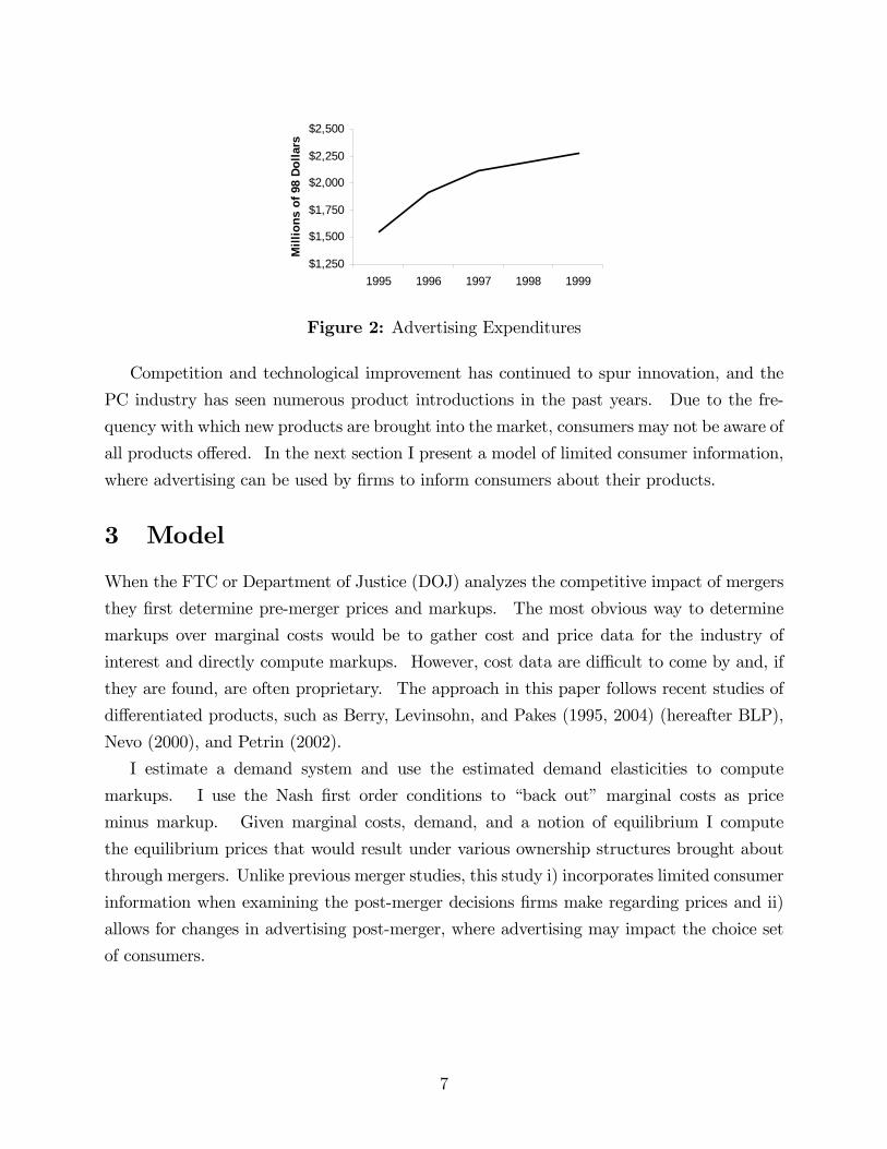
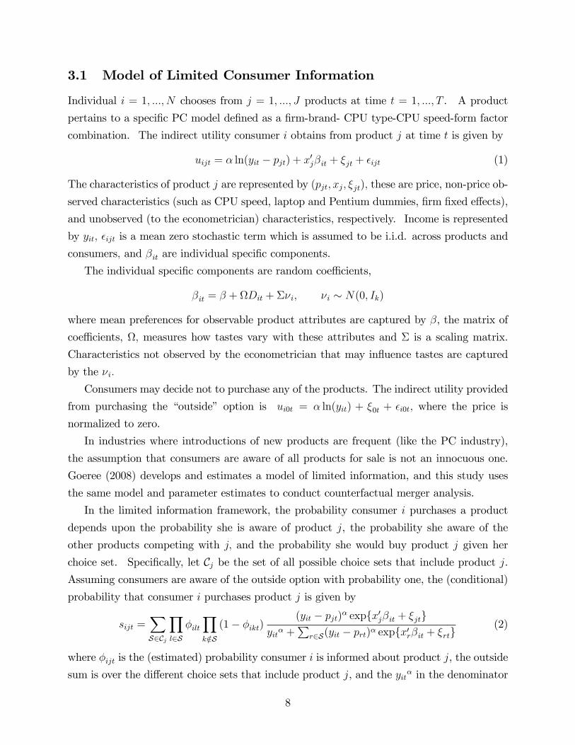
about their products. As Figures 1 and 2 illustrate, prices dropped from an average of

close to $2600 in early 1997 to just above $1500 in 1999, while advertising expenditures grew

by over $0.5 billion. Advertising has been an important dimension of competition in this

industry since its beginnings. Between 1995 and 1999, advertising expenditures grew by

nearly 100% to $2.3 billion. In 1998 over 36 million PCs were sold, generating over $62

billion in sales of which $2 billion was spent on advertising.

$1,500

$1,700

$1,900

$2,100

$2,300

$2,500

$2,700

1996

1997

1998

1999

2000

Ave

rage

 Pric

e (9

8$)

­1

1

3

5

7

9

11

13

Tota

l Uni

ts (i

n m

illio

ns)

Average Price Total Units Sold

Figure 1

9 I drew a sample of 3,000 individuals from the March CPS for each year. Quarterly income data wereconstructed from annual data and were de�ated using the Consumer Price Index from BLS. A few householdsreported an annual income below $5000. These households were dropped from the sample. Examination ofthe Simmons data indicate that purchases were made only by households with annual income greater than$5000, therefore eliminating very low income households should not a¤ect the group of interest.

6

$1,250

$1,500

$1,750

$2,000

$2,250

$2,500

1995 1996 1997 1998 1999M

illio

ns o

f 98 

Dol

lars

Figure 2: Advertising Expenditures

Competition and technological improvement has continued to spur innovation, and the

PC industry has seen numerous product introductions in the past years. Due to the fre-

quency with which new products are brought into the market, consumers may not be aware of

all products o¤ered. In the next section I present a model of limited consumer information,

where advertising can be used by �rms to inform consumers about their products.

3 Model

When the FTC or Department of Justice (DOJ) analyzes the competitive impact of mergers

they �rst determine pre-merger prices and markups. The most obvious way to determine

markups over marginal costs would be to gather cost and price data for the industry of

interest and directly compute markups. However, cost data are di¢ cult to come by and, if

they are found, are often proprietary. The approach in this paper follows recent studies of

di¤erentiated products, such as Berry, Levinsohn, and Pakes (1995, 2004) (hereafter BLP),

Nevo (2000), and Petrin (2002).

I estimate a demand system and use the estimated demand elasticities to compute

markups. I use the Nash �rst order conditions to �back out� marginal costs as price

minus markup. Given marginal costs, demand, and a notion of equilibrium I compute

the equilibrium prices that would result under various ownership structures brought about

through mergers. Unlike previous merger studies, this study i) incorporates limited consumer

information when examining the post-merger decisions �rms make regarding prices and ii)

allows for changes in advertising post-merger, where advertising may impact the choice set

of consumers.

7

3.1 Model of Limited Consumer Information

Individual i = 1; :::; N chooses from j = 1; :::; J products at time t = 1; :::; T . A product

pertains to a speci�c PC model de�ned as a �rm-brand- CPU type-CPU speed-form factor

combination. The indirect utility consumer i obtains from product j at time t is given by

uijt = � ln(yit � pjt) + x0j�it + �jt + �ijt (1)

The characteristics of product j are represented by (pjt; xj; �jt); these are price, non-price ob-

served characteristics (such as CPU speed, laptop and Pentium dummies, �rm �xed e¤ects),

and unobserved (to the econometrician) characteristics, respectively. Income is represented

by yit; �ijt is a mean zero stochastic term which is assumed to be i.i.d. across products and

consumers; and �it are individual speci�c components.

The individual speci�c components are random coe¢ cients,

�it = � + Dit + ��i; �i � N(0; Ik)

where mean preferences for observable product attributes are captured by �, the matrix of

coe¢ cients, ; measures how tastes vary with these attributes and � is a scaling matrix.

Characteristics not observed by the econometrician that may in�uence tastes are captured

by the �i:

Consumers may decide not to purchase any of the products. The indirect utility provided

from purchasing the �outside� option is ui0t = � ln(yit) + �0t + �i0t; where the price is

normalized to zero.

In industries where introductions of new products are frequent (like the PC industry),

the assumption that consumers are aware of all products for sale is not an innocuous one.

Goeree (2008) develops and estimates a model of limited information, and this study uses

the same model and parameter estimates to conduct counterfactual merger analysis.

In the limited information framework, the probability consumer i purchases a product

depends upon the probability she is aware of product j, the probability she aware of the

other products competing with j; and the probability she would buy product j given her

choice set. Speci�cally, let Cj be the set of all possible choice sets that include product j.Assuming consumers are aware of the outside option with probability one, the (conditional)

probability that consumer i purchases product j is given by

sijt =XS2Cj

Yl2S

�iltYk=2S

(1� �ikt)(yit � pjt)

� expfx0j�it + �jtgyit� +

Pr2S(yit � prt)� expfx0r�it + �rtg

(2)

where �ijt is the (estimated) probability consumer i is informed about product j, the outside

sum is over the di¤erent choice sets that include product j, and the yit� in the denominator

8

is from the outside option. I assume the � are distributed i.i.d. type I extreme value in

order to obtain simple expressions for choice probabilities.

Advertising may impact demand through the information technology function, �ijt. Sup-

pressing time notation, the advertising technology for product j for consumer i is given by

�ij =exp

� j + �ij

�1 + exp

� j + �ij

� (3)

The components of �ij that are the same for all consumers is given by

j =4P

m=1

ajm('m + �majm +f ) + #xagej :

The j term is a function of medium advertising (ajm) which may have di¤erent informa-

tional e¤ects across media (as measured by the parameters 'm and �m) and across �rms (as

measured by �rm �xed e¤ects f ).10 Finally, consumers may be more likely to know a

product the longer it has been on the market captured by # where xagej is the age of the PC

measured in quarters.

The �ij captures consumer information heterogeneity:

�ij =4P

m=1

ajm(�mDsi � + �im) + eD0

ie� ln�i � N(0; Im):

Medium advertising may have di¤erent e¤ects across consumers, where Dsi is vector of ob-

served consumer attributes from the Simmons data.11 The �mDsi term is the exposure of

individual i to medium m; and the � term measures how advertising exposure (measured by

ajm�mDsit) impacts the information technology. Consumers information may be di¤erent

even if they haven�t seen an advertisement, which may depend upon their own attributes

(where the eDi term is a subset of consumer characteristics). The �i vector are unobserved

(to the econometrician) consumer heterogeneity with regard to ad medium e¤ectiveness. I

assume � are independent of other unobservables.12

I assume the consumer purchases at most one good per period, that which provides the

10 I include �xed e¤ects for those �rms that o¤ered a product every quarter, but do not estimate a separate�xed e¤ect for each medium.11 Simmons data are used to identify �:

12 Notice �ij depends upon own product advertising only. I assume the probability a consumer is informedabout a product is (conditional on her attributes) independent of the probability she is informed about anyother product. Information provided (through advertising) for one product (or by one �rm) cannot �spillover�to another product (or to another �rm). That is, I assume product or group advertising for product r 6= jprovides no information about j.

9

highest utility from all the goods in her choice set.13 Let {i = (yi; Di; �i; �i) be the vector

of individual characteristics. The set of variables that results in the purchase of good j is

Rj � f{ : U({; pj; xj; aj; �j; �ij) � U({; pr; xr; ar; �r; �ir) 8r 6= jg: The market share ofproduct j is

sjt =

ZRj

dF (y;D; �; �; �) =

ZRj

sijdFy;D(y;D)dF�(�)dF�(�) (4)

where F (�) denotes the respective known distribution functions. The second equation followsfrom independence assumptions.14

3.2 Firm Behavior

I assume there are F �rms in an oligopolistically competitive industry and that they are non-

cooperative, Bertrand-Nash competitors. Each �rm produces a subset of the J products,

Jf . Suppressing time notation, the pro�ts of �rm f areXj2Jf

(pj �mcj)Msj(p; a) +Xj2Jf

�nhj (pnh)�

Xm

mcadjm(Xj2Jf

ajm)�Cf (5)

where sj is the vector of home market shares, which is a function prices and advertising for all

products; mcj is the marginal cost of production; �nhj is the gross pro�t (before advertising)

from sales to the non-home sectors; mcadjm is the marginal cost of advertising in medium m;

ajm is the number of medium m advertisements; and Cf are �xed costs of production. Thepotential market size, M, is given by the number of US households in a given period, as

reported by the Census Bureau.

Following BLP, I assume mcj are composed of unobserved (!j) and observed (wj) cost

characteristics:

ln(mcj) = w0j� + !j: (6)

13 This assumption may be questionable in markets where multiple purchase is common. However, itseems reasonable to restrict a consumer to purchase one computer per quarter. Hendel (1999) presents amultiple-choice model of PC purchases in the business sector.

14 The market shares must be simulated. As in BLP, the distribution of consumer demographics is anempirical one. As a result there is no analytical solution for predicted shares. Furthermore consumers maynot know all products for sale, but I don�t observe the choice set facing any one consumer. I implement thesolution provided in Goeree (2008) and simulate the choice set facing an individual. This eases computationburden signi�cantly. Instead of requiring 2J�1 purchase probability calculations for each individual (corre-sponding to each possible choice set) for each product, I need only compute the purchase probability for icorresponding to i�s simulated choice set for each product. See Goeree(2008) for details on the simulationtechnique.

10

Similarly, I assume mcadjm are composed of observed components, wadjm (such as the average

price of an advertisement),15 and unobserved components, � j :

ln(mcadjm) = wad0jm + � j � j � N(0; Im): (7)

I set the variance of � j to one for all media channels.

Given their products and the advertising, prices, and attributes of competing products,

�rms choose prices and advertising media levels simultaneously to maximize pro�ts. Firms

may sell to non-home sectors (such as the business, education, and government sectors).

Constant marginal costs imply pricing decisions are independent across sectors.16 Any

product sold in the home market sector will have prices that satisfy

sj(p; a) +Xr2Jf

(pr �mcr)@sr(p; a)

@pj= 0 (8)

In vector form, the J �rst-order conditions are

s��(p�mc) = 0

where �j;r = �@sr@pjIj;r with Ij;r an indicator function equal to one when j and r are produced

by the same �rm and zero otherwise. These FOC�s imply marginal costs given by

mc = p���1s (9)

However, an advertisement intended to reach a home consumer may impact sales in non-

home sectors. Optimal advertising choices must equate the marginal revenue of an additional

advertisement in all sectors with the marginal cost. Optimal advertising medium choices

ajm satisfy

MXr2Jf

(pr �mcr)@sr(p; a)

@ajm+mrnhj (p

nh) = mcadjm (10)

where mrnh is the marginal revenue of advertising in non-home market sectors.17

15 The advertising data include ad expenditures across ten media. The quarterly average ad price in mediagroup m is a weighted average of ad prices in the original categories comprising the group m. The weightsare �rm speci�c and are determined by the distribution of the �rms advertising across the original media.

16 There are reasons to believe that pricing decisions may not be independent across sectors. For instance,if the price of a particular laptop is lower for business, a consumer might buy the laptop from their businessaccount for use at home. Identi�cation of a model which includes pricing decisions across all sectors wouldrequire richer data for non-home sectors. Also, education, business, and government groups usually purchasemultiple PCs, which greatly complicates the model (Hendel, 1999). While the assumptions that I imposeimply independent pricing decisions, the estimates are sensible, and goodness-of-�t tests suggest the model�ts the data reasonably well.

17 I approximate the marginal revenue of advertising with mrnhj = �nhp pnhj +xnh0j �nhx , where characteristics

of product j sold in the non-home sector are price (pnhj ) and other observable characteristics (xnhj ) including

advertising, CPU speed, and non-PC �rm sales.

11

4 Estimation

Identi�cation Following the literature, I assume that the demand and pricing unob-

servables (evaluated at the true parameter values, �0) are mean independent of a set of

exogenous instruments; z :

E��j(�0) j z

�= E [!j(�0) j z] = 0: (11)

I do not observe �j or !j, but market participants do. This leads to endogeneity problems

because prices and ad choices are most likely functions of unobserved characteristics. A

solution to this problem involves instrumental variables.18 BLP show that variables that

shift markups are valid instruments for price in di¤erentiated products models. In a limited

information framework the components of z include the characteristics of all the products

marketed (the x vector), variables that determine production costs (the components of the

observed w vector that are not in x) and variables that determine advertising costs (the

components of wad).

The intuition to motive the advertising instruments follows Goeree(2008) and is similar to

that used by BLP to motivate the price instruments. Products which face more competition

(due to many rivals o¤ering similar products) will tend to have lower markups relative to

more di¤erentiated products. Advertising for j depends on j�s markup. As ad �rst order

conditions (FOC) in (10) indicate, a �rm will advertise a product more the more they make

on the sale of the product, ceteris paribus. The pricing FOCs in (8) show the optimal

price (and hence markup) for j depends upon characteristics of all of the products o¤ered.

Therefore, the optimal price and advertising depends upon the characteristics, prices, and

advertising of all products o¤ered. Note also that the level of advertising for j in media

m depends on the marginal cost of advertising in that media: Thus the instruments will

be functions of attributes, product cost shifters, and advertising cost shifters of all other

products.

I use an approximation to the optimal instruments presented in BLP(1999). I form

the approximation by evaluating the derivatives at the expected value of the unobservables

(� = ! = 0). The approximations are constructed so as to be highly correlated with the

relevant variables and are functions of exogenous data. Hence the exogenous instruments

will be consistent estimates of the optimal instruments. Details are provided in Appendix

A.

18 Berry (1994) was the �rst to discuss the implementation of instrumental variables methods to correctfor endogeneity between unobserved characteristics and prices. BLP provide an estimation technique. Mymodel and estimation strategy is in this spirit but is adapted to correct for advertising endogeneity.

12

Next, I present an informal discussion of how variation in the data identi�es the parame-

ters. The mean utility associated with purchasing a PC is chosen such that observed market

shares matches predicted market shares. If consumers were identical, then all variation in

sales would be driven by variation in product attributes. Variation in product market

shares corresponding to variation in the observable attributes of those products (such as

CPU speed) is used to identify the parameters of mean utility (�). Identi�cation of the taste

distribution parameters (�;) relies on information on how consumers substitute. Variation

in sales patterns over time as the set of available products change allows for identi�cation

of �. Also, I augment the market level data with micro data on �rm choice. The extra

information in the micro data allows variation in choices to mirror variation in tastes for

product attributes. Correlation between xjDi and choices identi�es the parameters.

If consumers were identical, then all variation in the information technology, and induced

variation in shares, would be driven by variation in advertising or the age of the PC. Variation

in sales corresponding to variation in PC age identi�es #. Variation in sales corresponding

to variation in advertising identi�es the other parameters of j. Returns to scale in media

advertising (�m) are identi�ed by covariation in sales with the second derivative of ajm.19

Identi�cation of �rm-�xed e¤ects (f ) are identi�ed in by (i) the total variation in sales of

all products sold by the �rm corresponding to variation in �rm advertising and (ii) in the

Simmons data by observed variation in �rm sales patterns corresponding to variation in �rm

advertising.

One major drawback of aggregate ad data is that I don�t observe variation across house-

holds in advertising exposure. Normally observed variation in market shares corresponding

to variation in household ad media exposure would be necessary to identify � and &. In

Goeree (2008) I show how to use the additional information in the Simmons data to aid

identi�cation. In short, variation in choices of media exposure corresponding to variation

in observable consumer characteristics (Dsi ) identi�es �. Variation in sales and ad exposure

(a0j�Dsi ) identi�es the e¤ect of ad exposure on the information set (&): The other parameters

of �ij which do not interact with advertising (e�) are separately identi�ed from due to

nonlinearities.20

19 There is not enough variation in the ad data to estimate ' and � e¤ects for all media separately. Iestimate these parameters for the tv medium and for the combination of newspaper and magazine media.

20 The parameters on group advertising (�1 and �2) are identi�ed by observed variation in expenditureson group advertisements (adm) with the number of products in the group and by functional form.

13

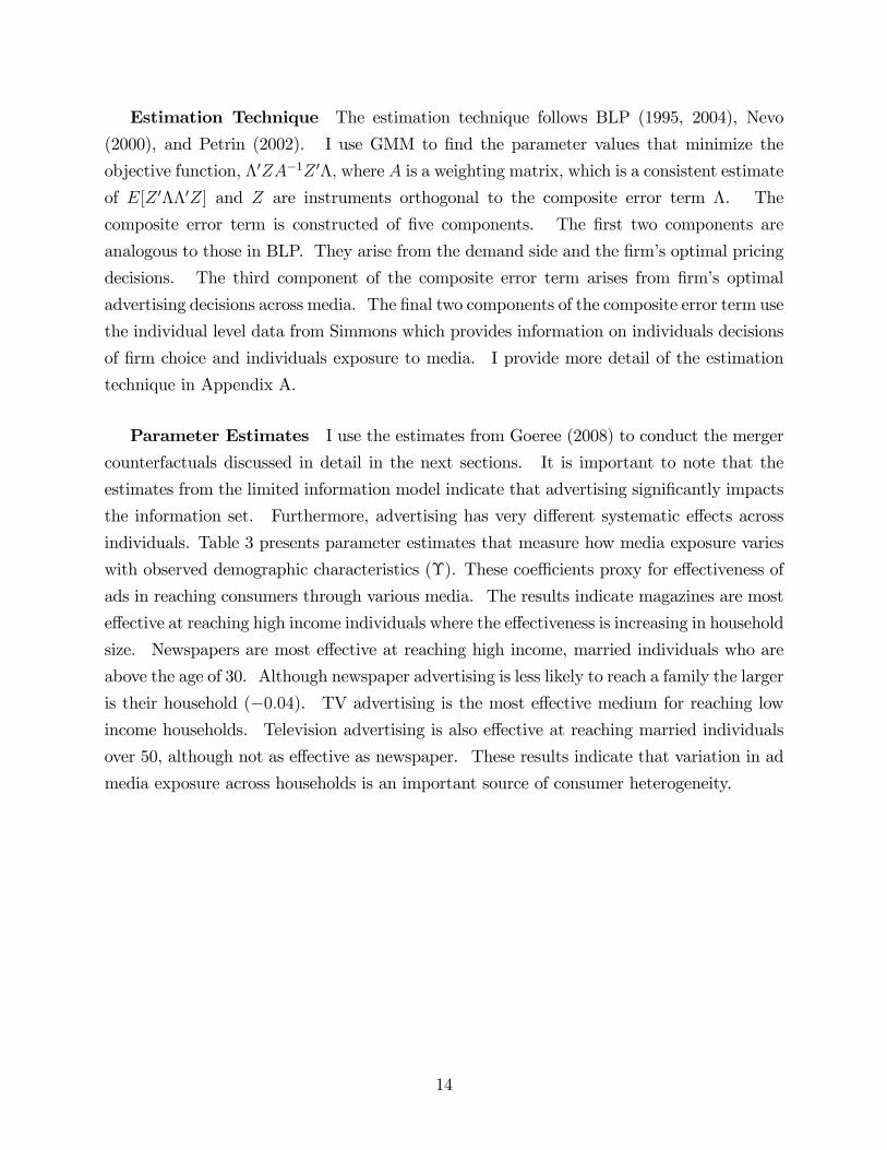
Estimation Technique The estimation technique follows BLP (1995, 2004), Nevo

(2000), and Petrin (2002). I use GMM to �nd the parameter values that minimize the

objective function, �0ZA�1Z 0�; where A is a weighting matrix, which is a consistent estimate

of E[Z 0��0Z] and Z are instruments orthogonal to the composite error term �. The

composite error term is constructed of �ve components. The �rst two components are

analogous to those in BLP. They arise from the demand side and the �rm�s optimal pricing

decisions. The third component of the composite error term arises from �rm�s optimal

advertising decisions across media. The �nal two components of the composite error term use

the individual level data from Simmons which provides information on individuals decisions

of �rm choice and individuals exposure to media. I provide more detail of the estimation

technique in Appendix A.

Parameter Estimates I use the estimates from Goeree (2008) to conduct the merger

counterfactuals discussed in detail in the next sections. It is important to note that the

estimates from the limited information model indicate that advertising signi�cantly impacts

the information set. Furthermore, advertising has very di¤erent systematic e¤ects across

individuals. Table 3 presents parameter estimates that measure how media exposure varies

with observed demographic characteristics (�). These coe¢ cients proxy for e¤ectiveness of

ads in reaching consumers through various media. The results indicate magazines are most

e¤ective at reaching high income individuals where the e¤ectiveness is increasing in household

size. Newspapers are most e¤ective at reaching high income, married individuals who are

above the age of 30. Although newspaper advertising is less likely to reach a family the larger

is their household (�0:04). TV advertising is the most e¤ective medium for reaching low

income households. Television advertising is also e¤ective at reaching married individuals

over 50, although not as e¤ective as newspaper. These results indicate that variation in ad

media exposure across households is an important source of consumer heterogeneity.

14

 MediaMagazine Newspaper Television Radio

Variable Coefficient Std. Error Coefficient Std. Error Coefficient Std. Error Coefficient Std. Errorconstant ­1.032 ** (0.040) ­0.973 ** (0.040) ­1.032 ** (0.041) ­1.000 ** (0.043)30to50 (=1 if 30<age<50 ­0.042 * (0.025) 0.207 ** (0.025) 0.019 (0.025) ­0.030 * (0.025)50plus (=1 if age>50) 0.005 (0.025) 0.541 ** (0.025) 0.193 ** (0.025) ­0.245 ** (0.025)married (=1 if married) ­0.022 * (0.018) 0.187 ** (0.018) 0.075 ** (0.018) ­0.011 (0.018)hh size (household size) 0.040 ** (0.006) ­0.038 ** (0.006) 0.018 ** (0.006) 0.012 * (0.006)inclow (=1 if income<$60,000) ­0.194 ** (0.021) ­0.251 ** (0.021) 0.114 ** (0.021) ­0.117 ** (0.022)inchigh (=1 if income>$100,000) 0.153 ** (0.029) 0.127 ** (0.028) ­0.025 (0.030) 0.069 ** (0.030)malewh (=1 if male and white) ­0.078 ** (0.018) 0.002 (0.018) ­0.019 * (0.018) 0.006 (0.018)eduhs (=1 if highest edu 12 years) ­0.102 ** (0.026) ­0.338 ** (0.026) 0.296 ** (0.027) 0.076 ** (0.027)eduad (=1 if highest edu 1­3 college) 0.032 * (0.028) ­0.166 ** (0.027) 0.278 ** (0.028) 0.115 ** (0.029)edubs (=1 if highest edu college grad) ­0.024 (0.025) ­0.063 ** (0.024) 0.145 ** (0.025) 0.081 ** (0.026)edusp (education if <11) ­0.028 ** (0.003) ­0.069 ** (0.003) 0.034 ** (0.003) ­0.014 ** (0.003)Notes: Estimates include time dummies.   ** indicates significant at the 5% level; * significant at the 10% level.

Table 3: Media Exposure Parameter Estimates

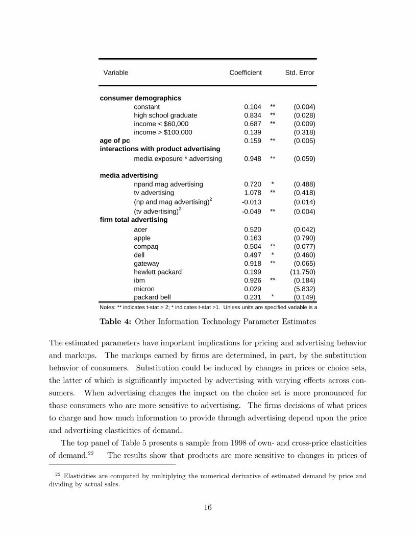
Table 4 shows that the variation in ad exposure translates into variation in information

sets with a positive and highly signi�cant estimate for & (0.948). Parameter estimates of e�suggest other means of information provision, such as word-of-mouth or experience, play a

role in informing certain types of consumers. The coe¢ cient on income less than $60,000

(0:69) indicates these individuals are likely to be informed about 41% of the products without

seeing an ad. Whereas having a high income is not signi�cantly di¤erent from having a

middle income, in terms of being informed without seeing an ad. In addition, the probability

of being informed without seeing any advertising is higher for high-school grads relative to

non-graduates.

Consumers are signi�cantly more likely to know a PC the longer it has been on the market

(0:16): There are decreasing returns to advertising in the TV (�0:05) and newspapers andmagazines (�0:01) media, but they are decreasing at a faster rate for TV. Estimates of �rm�xed e¤ects interacted with total advertising () indicate that some �rms are more e¤ective

at informing consumers through advertising. Most notably ads by Compaq, Dell, Gateway,

IBM and Packard Bell are signi�cantly more e¤ective, which could be due to di¤erences in

advertising techniques across �rms.21

21 I present the parameter estimates for the remaining parameters of the utility and cost functions inAppendix B.

15

Variable Coefficient Std. Error

consumer demographicsconstant 0.104 ** (0.004)high school graduate 0.834 ** (0.028)income < $60,000 0.687 ** (0.009)income > $100,000 0.139 (0.318)

age of pc 0.159 ** (0.005)interactions with product advertising

media exposure * advertising 0.948 ** (0.059)

media advertisingnpand mag advertising 0.720 * (0.488)tv advertising 1.078 ** (0.418)(np and mag advertising)2 ­0.013 (0.014)(tv advertising)2 ­0.049 ** (0.004)

firm total advertisingacer 0.520 (0.042)apple 0.163 (0.790)compaq 0.504 ** (0.077)dell 0.497 * (0.460)gateway 0.918 ** (0.065)hewlett packard 0.199 (11.750)ibm 0.926 ** (0.184)micron 0.029 (5.832)packard bell 0.231 * (0.149)

Notes: ** indicates t­stat > 2; * indicates t­stat >1.  Unless units are specified variable is a dummy.

Table 4: Other Information Technology Parameter Estimates

The estimated parameters have important implications for pricing and advertising behavior

and markups. The markups earned by �rms are determined, in part, by the substitution

behavior of consumers. Substitution could be induced by changes in prices or choice sets,

the latter of which is signi�cantly impacted by advertising with varying e¤ects across con-

sumers. When advertising changes the impact on the choice set is more pronounced for

those consumers who are more sensitive to advertising. The �rms decisions of what prices

to charge and how much information to provide through advertising depend upon the price

and advertising elasticities of demand.

The top panel of Table 5 presents a sample from 1998 of own- and cross-price elasticities

of demand.22 The results show that products are more sensitive to changes in prices of

22 Elasticities are computed by multiplying the numerical derivative of estimated demand by price anddividing by actual sales.

16

computers with similar characteristics. Among PC�s that have a windows operating system,

form factor plays a strong role in substitution patterns. For example, Compaq Armada

laptop is most sensitive to changes in prices of other laptops rather than to changes in other

Compaq non-laptop computers. While Apple computers are most sensitive to changes in

the prices of other Apple computers implying there is less substitution across platforms.

Apple Apple Compaq Compaq Dell HP HP IBM IBMPowerBook* Power Mac Armada* Presario Latitude* Omnibook* Pavilion PC Thinkpad*

price elasticitiesPowerBook* ­12.861 0.0692 0.0243 0.0287 0.0170 0.0219 0.0213 0.0182 0.0165Power Mac 0.0856 ­11.097 0.0202 0.0222 0.0196 0.0202 0.0248 0.0298 0.0364Armada 7xxx* 0.0150 0.0107 ­5.7066 0.0193 0.0606 0.0209 0.0203 0.0162 0.0426Presario 2xxx 0.0122 0.0272 0.0125 ­3.6032 0.0230 0.0272 0.0308 0.0348 0.0385Latitude XPI* 0.0263 0.0274 0.0357 0.0261 ­5.5701 0.0225 0.0217 0.0394 0.0453Omnibook 4xxx* 0.0179 0.0147 0.0363 0.0298 0.0228 ­5.6501 0.0269 0.0222 0.0499Pavilion 6xxx 0.0118 0.0212 0.0153 0.0336 0.0167 0.0227 ­5.1178 0.0396 0.0359PC 3xxx 0.0137 0.0322 0.0137 0.0381 0.0153 0.0148 0.0325 ­3.2626 0.0215Thinkpad 7xxx* 0.0330 0.0192 0.0376 0.0195 0.0304 0.0425 0.0297 0.0291 ­6.9745

advertising semi­elasticitiesPowerBook* 0.0076 ­0.0057 ­0.0142 ­0.0110 ­0.0044 ­0.0139 ­0.0166 ­0.0072 ­0.0097Power Mac ­0.0057 0.0215 ­0.0147 ­0.0273 ­0.0179 ­0.0136 ­0.0243 ­0.0263 ­0.0213Armada 7xxx* ­0.0616 ­0.0564 0.0017 ­0.0057 ­0.0314 ­0.0625 ­0.0441 ­0.0684 ­0.0948Presario 2xxx ­0.0779 ­0.0827 ­0.0060 0.0120 ­0.0208 ­0.1092 ­0.1413 ­0.0825 ­0.0830Latitude XPI* ­0.0233 ­0.0114 ­0.0278 ­0.0274 0.0230 ­0.0380 ­0.0239 ­0.0199 ­0.0438Omnibook 4xxx* ­0.0034 ­0.0042 ­0.0039 ­0.0043 ­0.0064 0.0054 ­0.0021 ­0.0030 ­0.0044Pavilion 6xxx ­0.0036 ­0.0045 ­0.0038 ­0.0082 ­0.0051 ­0.0066 0.0101 ­0.0143 ­0.0054PC 3xxx ­0.0076 ­0.0085 ­0.0082 ­0.0161 ­0.0182 ­0.0127 ­0.0194 0.0095 ­0.0029Thinkpad 7xxx* ­0.0107 ­0.0088 ­0.0168 ­0.0164 ­0.0185 ­0.0127 ­0.0196 ­0.0020 0.0089Notes: A * indicates a laptop.  For price elasticities, cell entries i,j where i ,indexes row and j  column, give the percentage change in market shareof brand I with a 1% change in the price of j. Each entry represents the median of the elasticities from 1998. For advertising elasticities, cell entries i,jgive the percent change in the market share of i  with a $1000 increase in the advertising of j.

Table 5: A Sample from 1998 of Estimated Price and Advertising Elasticities

Estimated advertising demand elasticities indicate that, for some �rms, advertising for

one product has negative e¤ects on other products sold by that �rm but it is less negative

than for some of the rival products.23 The lower panel presents a sample from 1998.

Each semi-elasticity gives the percentage change in the market share of the row computer

associated with a $1000 increase in the (estimated) advertising of the column computer. For

instance, a $1000 increase in advertising for Apple Power Mac results in a decreased market

share of around 0.1% for Compaq Presario but has very little e¤ect on the market share

for Apple PowerBook. In contrast, an increase in advertising for HP Omnibook has a large

e¤ect (relative to increase in own market share) on the market share for HP Pavilion.

23 The model does not allow advertising for one product (or by one �rm) to have positive spillovers toanother product. Hence, the cross-product advertising e¤ects (the o¤-diagonals in the lower panel of Table5) are all negative. The diagonal elements report the increase in market share from own-advertising. Forexample, an increase of $1000 for advertising on Dell Latitude results in an increased market share of 0.02%.

17

Median Percentage MarkupAverage Price Ad to Sales Ratio over marginal costs including ad costs

Total Industry $2,239 3.4% 15% 10%

Top 6 firms $2,172 9.1% 17% 12%

Apple $1,859 5.3% 16% 9%Compaq $2,070 2.4% 23% 16%Gateway $2,767 5.6% 12% 10%Hewlett­Packard $2,203 17.7% 16% 10%IBM $2,565 20.1% 16% 10%Packard Bell ­ NEC $2,075 7.2% 16% 11%Notes: ad to sales ratios are annual averages and are from LNA and include all sectors (home, business, education, government).markups are the median (price­marginal costs)/price across all products. The last column is determined from estimated markupsand estimated effective product advertising in the home sector.

Table 6: Estimated Median Markups

I use estimated demand to infer marginal costs and markups as shown in Table 6. The

median markup charged by PC �rms is 15% over marginal costs of production and 10%

over per unit production and (estimated) advertising costs. As the �rst two rows show, the

top �rms have higher than average markups and advertising expenditures relative to the

industry. Indeed the non-top �rms�average median markup is much lower, 12%, with an

ad-to-sales ratio of about 2%. The �nal column shows that, even after controlling for the

fact that the top �rms advertise more, they continue to earn higher than average markups.

In 1998 the median industry markup was 19% over costs with the top �rms earning a 22%

markup. Overall industry and top �rm markups were increasing over the period.

5 Post Merger Equilibrium

In this section I present the results from two counterfactual merger simulations: a merger

between HP and Compaq and a hypothetical merger between IBM and Dell. All post-merger

computations use the estimates from the limited information model of demand and supply

presented in the above section. I simulate post-merger equilibria under two assumptions of

post-merger behavior on part of the �rms. First, I compute the new price equilibrium under

the assumption that advertising choices remain at pre-merger levels. That is, I do not allow

�rms to reoptimize over advertising choices. This is used as the benchmark case. Notice

that this benchmark case will provide an accurate picture of the post-merger industry only

if �rms do not change their advertising strategy or if advertising does not impact demand.

18

I compare the benchmark case to the new price and advertising equilibrium that arises

post-merger allowing �rms to reoptimize over both prices and advertising.

For the �rst two parts of the analysis I use estimated costs and, hence, assume the cost

structure is the same both before and after the merger. Firms may experience decreased

costs (synergies) as a result of a merger. Therefore, in the �nal part of the analysis (following

Nevo, 2000) I determine the magnitude of cost savings that would be necessary to return to

the pre-merger price and advertising equilibrium.

I assume post-merger market conduct is the same as pre-merger, and use the estimated

pre-merger parameters to simulate the (counterfactual) post-merger equilibrium. The pre-

dicted post-merger equilibrium price ppost solves

ppost = cmc+�post(ppost)�1s(ppost) (12)

where the matrix �post is constructed to re�ect post-merger ownership structure, cmc are thepredicted marginal costs and ppost is the vector of post-merger predicted equilibrium prices.

The predicted post-merger advertising levels solve (10) under the new ownership structure,

holding marginal costs constant at their estimated levels. The post-merger equilibrium

levels of prices and advertising are simulated jointly using the data from the last quarter of

1998.

5.1 Advertising and Market Power

Table 7 presents �rm and industry level changes in prices, advertising, and markups after

the mergers. The �rst column presents average percentage changes in prices under the

assumption that post-merger advertising levels are unchanged. Predicted price changes are

higher for the merging �rms, especially under the Compaq-HP merger. In addition all �rms

increase their prices under the HP-Compaq merger. We might expect prices to increase for

all �rms in the industry, as the industry is more concentrated allowing �rms to exercise more

market power. However, counter to intuition, under the Dell-IBM merger some �rms charge

lower average prices and overall industry prices experience only a small increase in price

(0.2%). This unexpected result may be due to the assumption that �rms leave advertising

expenditures unchanged.

19

Optimizing Variable:  Price only Price and advertising% change % change Difference in % change Estimatedin prices in prices price changes in ads % Markups

Compaq­HP merger:Apple 2.1% 5.8% 3.6% 0.3% 12%Compaq­HP 18.9% 18.4% ­0.5% 10.8% 31%Dell 2.9% 2.9% 0.0% 3.3% 13%IBM 5.8% 7.8% 2.0% 0.2% 25%

Industry Total 6.9% 9.3% 2.4% 3.3% 24%

Dell­IBM merger:

Apple 0.0% 4.8% 4.8% 0.2% 13%Compaq ­0.1% 7.8% 7.8% 2.4% 24%Dell­IBM 1.3% 5.9% 4.6% 0.9% 13%Hewlett­Packard 0.5% 4.8% 4.3% 8.5% 20%

Industry Total 0.2% 6.1% 5.9% 1.8% 21%

Note: Each entry represents the average percentage change in the final quarter of 1998. Estimated % Markups include ad costs

Table 7: Firm and Industry Post-Merger Results

The second and third columns present results based on the assumption that �rms choose

new prices and advertising levels after the merger. As the second column shows, the pricing

outcome is more intuitive. All �rms increase their prices as industry concentration grows.

The overall price increase in the industry is 9% and 6% under the HP-Compaq and Dell-IBM

mergers, respectively. Surprisingly, Dell-IBM do not raise prices as much as Compaq under

the Dell-IBM merger. The �rst column of Table 8 provides a breakdown of price changes

for selected products. As the table indicates, price increases are greatest for the HP and

IBM products under their respective mergers. One possible reason for this distribution is

that both HP and IBM have lower pre-merger prices than their merging counterparts. As

the third column of Table 7 indicates, prices are 2% and 6% higher under the HP-Compaq

and Dell-IBM mergers respectively relative to when �rms don�t reoptimize over advertising.

The fourth column presents percentage changes in advertising. All �rms choose to

advertise more in both post-merger environments. Advertising increases by 3.3% under the

HP-Compaq merger and 1.8% under the Dell-IBM merger. Prior to merging HP-Compaq

have a combined ad-to-sales ratio of 7%, while Dell-IBM�s is on the order of 14%. HP-

Compaq increases their advertising by 10% (or $75 million) after the merger, yielding a

post-merger ad-to-sales ratio of 20%.24 Dell-IBM increases their advertising by 0.9% (or

$12 million) post-merger, yielding a post-merger ad-to-sales ratio of 22%. It is interesting

that post-merger ad-to-sales ratios are similar for the merging �rms.

24 This is calculated using the post-merger shares, which are lower than pre-merger combined shares.

20

Column two of Table 8 provides an idea of how these advertising changes are distributed

across the products o¤ered by the merging �rms. The table shows that advertising increases

are larger for HP under the �rst merger �the more advertising intensive pre-merger �rm.

While under the Dell-IBM merger, advertising increases are greatest for the Dell products �

the less advertising intensive pre-merger �rm. These results suggest that knowing a �rm�s

pre-merger ad-to-sales ratio is not su¢ cient to predict post-merger advertising choices.

% change in % change in EstimatedPrices Advertising  % Markups

Compaq­HP MergerCompaq Presario Notebook* 9% 0% 22%Compaq Presario 9% 3% 20%HP OmniBook* 22% 67% 79%HP Pavilion 9% 65% 18%

Dell­IBM Merger:Dell Dimension 4% 1% 18%Dell Latitude* 4% 10% 40%IBM Aptiva 8% 0% 18%IBM Thinkpad* 8% 0% 92%Notes: Percentage changes are averages over all quarters.

Table 8: Post Merger Results for Selected Products

The �fth column of Table 7 presents a breakdown of post-merger markup percentages,

which include advertising costs. The industry average markup is higher (24%) relative to

pre-merger markups (10%) and post-merger price only markups (20%). The percentage

markups for Compaq-HP is about 50% higher than pre-merger levels, while for Dell-IBM it

is roughly equivalent.

The results suggest that �rms will charge higher prices in conjunction with more adver-

tising. Markups are about 10% higher on average when �rms are permitted to reoptimize

over advertising choices relative to optimizing over price only. Part of the post-merger higher

markup is due to industry concentration, and part is due to the e¤ect of advertising in this

industry. If the �rms were prohibited from changing their advertising, the industry would

look much more competitive. The results indicate that advertising is used to strategically

provide information, which reduces competition in the market.

The above analysis assumes costs do not change after the mergers. We may expect

there to be some synergies between companies resulting in decreased post-merger costs. I

21

calculated the percentage change in costs that would induce post-merger prices to equal

pre-merger prices under the �rst scenario of post-merger behavior (i.e., assuming �rms do

not reoptimize of ad expenditures post-merger). I do not make any assumptions regarding

which products of the acquiring �rms would enjoy cost reductions. The median percentage

changes are given in Table 9. The results indicate that a cost savings of 4% for HP-Compaq

is enough to reach pre-merger equilibrium prices. The cost savings would be mostly on HP

products. Even smaller costs savings, 2.7%, are enough to keep prices constant at pre-merger

levels for the merger of Dell and IBM. Under the Dell-IBM merger, cost savings are spread

more evenly over the products of both �rms, relative to the HP-Compaq outcome, but are

still more intense for Dell products. In addition, the costs savings are not of an unattainable

magnitude. HP and Compaq or Dell and IBM may experience a reduction in costs of close

to 4% and 3% respectively after merging. (more analysis of the results forthcoming...)

Compaq and HP Dell and IBMMerger Merger

Compaq Presario Notebook* ­2.95% 0.00%Compaq Presario ­4.67% 0.00%Dell Dimension 0.00% ­3.32%Dell Latitude* 0.00% ­2.91%HP OmniBook* ­10.41% 0.00%HP Pavilion ­5.35% 0.00%IBM Aptiva 0.00% ­5.03%IBM Thinkpad* 0.00% ­1.85%

Median over all products:Compaq and HP ­4.28%Dell and IBM ­2.72%Notes: Percentage changes are medians over all quarters.

Table 9: Reduction in Marginal Costs Necessary to O¤set Price Increases

5.2 Consumer Surplus and Pro�ts

Remarking on the HP-Compaq merger, a research fellow at Gartner noted, �There�s nothing

good for the consumers. They�ve eliminated one of two �ercely competitive brands in the

market. And what that means generally is higher prices and less choice.� The previous

subsection uses the structural estimates to produce a counterfactual of what the market

equilibrium would look like under the merger. In this section, I examine the impact of the

mergers on consumer surplus and pro�ts to provide further insight into the social welfare

e¤ects of these mergers.

22

Consumers face di¤erent prices and (possibly) di¤erent choice sets as a result of a merger.

Evaluating the change in utility generated by di¤erences in choice sets is possible since

preferences are de�ned over characteristics. I use compensating variation to measure changes

in consumer welfare. Compensating variation is the amount of money an individual would

need to be compensated at the new equilibrium prices and choice set to be as well o¤ as

they were under the pre-merger equilibrium. If household welfare is improved as a result of

the merger, the expected compensating variation measure is negative.

Compensating variation for individual i, cvi; is implicitly de�ned by

Maxj2Jprei

U(yi � pprej ) = Maxj2Jposti

U(yi � ppostj � cvi; ) (13)

where the superscripts �pre�and �post�are used to distinguish the original versus the new

conditions associated with the merger. Recall, consumers may not know all products avail-

able to them, Ji denotes the choice set facing consumer i.25 The pre- and post- merger

choice set may di¤er because the equilibrium level of advertising may change. Under assump-

tions of full information, the e¤ects on consumer welfare (as measured by the area under the

Hicksian or Marshallian demand curves) will be understated.

The resulting compensating variation is a random variable, which will depend upon �

in a nonlinear fashion. I am interested in the expected value of this random variable,

E(cv). Since marginal utility of income varies with income and prices there is no closed

form solution for E(cv): I simulate E(cv) using a procedure developed by McFadden (1999).

The simulation requires sampling from the underlying distribution of errors and employing a

numerical algorithm to solve for the implicitly de�ned cv as given in equation (13). I compute

cvi for R draws from the underlying distribution of errors. Mean compensating variation

for an individual is the average over these draws.26 I average across the sample to obtain

the mean compensating variation for the population. The change in welfare is computed by

25 The choice set for an individual is determined by comparing the value of the advertising technology,�ij ; to a draw from a uniform distribution. The advertising technology is evaluated at the estimated valueof the parameters and equilibrium advertising levels. If the uniform draw is larger, the product is not inthe choice set. If the uniform draw is smaller the product is in the choice set.Speci�cally, the pre-merger choice set is constructed as follows: given �ij(b�; apre) and a draw from a

uniform, uij ; construct a J dimensional Bernoulli vector, bi: This de�nes the choice set, where the jthelement is determined according to

bij =

�1 if �ij > uij0 if �ij < uij

analogously for the post-merger choice set.

26 McFadden (1999) demonstrates in a monte-carlo experiment that the number of iterations required toobtain a 5% root mean squared error when � are distributed extreme value 755. For this reason I chooseR = 755:

23

comparing consumer and producer welfare across the two economic environments. For each

merger, I calculate two compensating variations: one in which advertising is not a strategic

variable and one in which it is. I compare consumer welfare to pre-merger welfare under

both environments. (Consumer surplus and pro�t results are forthcoming...)

6 Conclusions

In markets characterized by rapid change consumers may not know every available product.

Currently, antitrust authorities evaluate the impact of mergers under the assumption that

consumers know all products for sale when making their purchases. This paper considers the

strategic motives of �rms to provide information via advertising when consumers may have

limited information. Speci�cally, I use the estimated parameters from a structural model of

limited information presented in Goeree (2008) to simulate post-merger equilibrium price and

advertising levels. I calculate the e¤ect of mergers on the pro�ts of merging and non-merging

�rms as well as the cost-synergies necessary to o¤set losses. I am able to decompose the

post-merger change in prices and markups into the changes due to increased concentration

and the changes due to the in�uence of information provision. The post-merger equilibrium

results indicate advertising can be used to increase market power, which suggests revisions to

the current model used by antitrust authorities to determine market power in antitrust cases.

Furthermore, the results suggest that the extent to which �rms are able to increase their

markup from strategic information provision depends in part on their pre-merger combined

ad-to-sales ratio, but also on the distribution of products within the merged entity.

24

References

Ackerberg, Daniel (2003) �Advertising, Learning, and Consumer Choice in ExperienceGoods Markets: A Structural Empirical Examination,�International Economic Review44:1007-1040.

Anand, Bharat and Ron Shachar (2001) �Advertising, the Matchmaker,� HarvardBusiness School Working Paper No. 02-057.

Anderson, Simon, A. de Palma, and J.F. Thisse (1989) �Demand for Di¤erentiatedProducts, Discrete Choice Models, and the Characteristics Approach,�Review of Eco-nomic Studies 56: 21-35.

Anderson, Simon, A. de Palma, and J.F. Thisse (1992) Discrete Choice Theory ofProduct Di¤erentiation, Cambridge: MIT Press.

Baker, J. and T. Bresnahan (1985) �The Gains from Merger or Collusion in ProductDi¤erentiated Industries,�The Journal of Industrial Economics, 33(4): 427-444.

Berry, Steven (1994) �Estimating Discrete Choice Models of Product Di¤erentiation,�Rand Journal of Economics 25(2): 242-262.

Berry, Steven, James Levinsohn and Ariel Pakes (2004) �Di¤erentiated Products De-mand Systems from a Combination of Micro and Macro Data: The New Car Market,�Journal of Political Economy 112(1,1): 68-105.

Berry, Steven and Ariel Pakes (1993) �Some Applications and Limitations of RecentAdvances in Empirical Industrial Organization: Merger Analysis,�American EconomicReview 83(2): 247-252.

Bresnahan, T. and S. Greenstein, (2000) �Technological Competition and the Structureof the Computer Industry,�Journal of Industrial Economics

Bresnahan, T., S. Stern, and M. Trajtenberg (1997) �Market Segmentation and theSources of Rents from Innovation: Personal Computers in the Late 1980s,�Rand Jour-nal of Economics 28(0): S17-S44.

Chamberlain, G. (1987) �Asymptotic E¢ ciency in Estimation with Conditional Mo-ment Restrictions,�Journal of Econometrics 34: 305-344.

Erdem, Tulin and Michael Keane (1996) �Decision-making Under Uncertainty: Cap-turing Dynamic Brand Choice Processes in Turbulent Consumer Goods Markets,�Marketing Science 15(1): 1-20.

Genakos, Christos (2004) �Di¤erential Merger E¤ects: The Case of the Personal Com-puter Industry,�mimeo, London Business School.

Goeree, Michelle S. (2002) �Informative Advertising and the U.S. Personal ComputerMarket: A Structural Empirical Examination,�University of Virginia Dissertation

25

Goeree, Michelle S. (2008) �Limited Information and Advertising in the US PersonalComputer Industry,�Econometrica 76(5):1017�1074.

Gourieroux, Christian, et al. (1987) �Generalized Residuals,�Journal of Econometrics,34: 5-32.

Grossman, G. and Carl Shapiro (1984) �Informative Advertising with Di¤erentiatedProducts,�Review of Economic Studies 51: 63-82.

Hausman, J., G. Leonard, and J. Zona (1994) �Competitive Analysis with Di¤erenti-ated Products,�Annales D�Economie et de Statistique 34: 159-180.

Hendel, I. (1999) �Estimating Multiple-Discrete Choice Models: An Application toComputerization Returns,�Review of Economic Studies 66(2): 423-46

McFadden, Daniel (1999) �Computing Willingness-to-Pay in Random Utility Models,�in J. Moore, R. Riezman, and J. Melvin (eds.), Trade, Theory and Econometrics:Essays in Honor of John S. Chipman, Routledge.

Nevo, Aviv (2000) ��Mergers with Di¤erentiated Products: The Case of the Ready-to-Eat Cereal Industry,�Rand Journal of Economics 31(3): 395-421.

Nevo, Aviv (2002) �New Products, Quality Changes and Welfare Measures Computedfrom Estimated Demand Systems,�Review of Economic Studies.

Pakes, Ariel and David Pollard (1989) �Simulation and the Asymptotics of Optimiza-tion Estimators,�Econometrica 57(5): 1027-1057.

Petrin, Amil (2002) �Quantifying the Bene�ts of New Products: The Case of theMinivan,�Journal of Political Economy 110(4):705-729.

Shapiro, C. (1996), �Mergers with Di¤erentiated Products,�Antitrust, 10(2), 23-30.

Small, Kenneth, and Harvey Rosen (1981) �Applied Welfare Economics with DiscreteChoice Models,�Econometrica 49: 105-130.

Werden, G.J. (1997) �Simulating the E¤ects of Di¤erentiated Products Mergers: APractictioners�Guide,�Proceedings of the NE-165 Conference.

Werden, G.J. and L.M. Froeb (1994) �The E¤ects of Mergers in Di¤erentiated Prod-ucts Industries: Logit Demand and Merger Policy,�Journal of Law, Economics, andOrganization, 194, 407-26.

Willig, R.D. (1991), �Merger Analysis, Industrial Organization Theory, and the MergerGuidelines,�Brookings Papers on Economic Activity, Microeconomics, 281-332.

26

Appendices

A Estimation DetailsI use macro product data, ad data, and the CPS consumer data in the �rst three sets ofmoments. I use micro consumer data in the last two sets of moments. Under the assumptionthat the data are the equilibrium outcomes, the parameters are estimated by GMM. I use�ve �sets�of moments to construct a composite error term. The �rst two sets of momentsare analogous to those in BLP.

I restrict the model predictions for product j�s market share to match observed marketshares. Using a contraction mapping suggested by Berry (1994) I compute the vector � (�),which is the implicit solution to Sobst � st(�; �) = 0, and use it to solve for the demand sideunobservable, �jt: The �rst moment unobservable is �jt = �jt(S; �)� x0j�:

The second set of moments arises from optimal pricing decisions. I assume marginalcosts of production, mcj, are composed of unobserved (!jt) and observed characteristics(wjt), where ln(mcj) = w0j� + !j: I use the I use the demand system estimates to computemarginal costs to obtain the cost side unobservable, !jt: The second moment unobservableis ! = ln(p��(�; �)�1s(�; �))� w0�:

The third set arises from �rms optimal advertising decisions. Some �rms choose notto advertise some products in some media. To allow for corner solutions, I use the marginalcosts associated with advertising and the advertising interior FOCs to construct a tobitmaximum likelihood function. I follow Gourieroux et al.(1987) to construct the advertisingresiduals used in the third set of advertising moments. The generalized residual for the jthobservation is

e� jm(b�) = E[� jm(b�) j ajm] = fmrjm1(ajm > 0)� �normal(fmrjm)1� �(fmrjm) 1(ajm = 0)

where � are the parameters of the tobit likelihood function and b� its maximum likelihoodestimator. The (third set of) moments express an orthogonality between the generalizedresiduals and the instruments.

The fourth set of moments use the Simmons micro data to construct �rm choice micromoments. Let Bi be a F � 1 vector of �rm choices for individual i and bi its realizationwhere bif = 1 if a brand produced by f was chosen. Then the �rm choice residual isthe di¤erence between the vector of observed choices and the model prediction given theparameters Bi(�; �) = bi � E�;�E[Bi j Ds

i ; �; �]: The population restriction for the micromoment is E[Bi(�; �) j (x; �)] = 0:

The �fth set of moments uses the Simmons data and matches the model�s predictionsfor exposure to mediam (conditional on observed characteristics) to observed exposure. Themedia exposure residual for i in medium m is de�ned as the di¤erence between the vectorof observed exposure and the prediction given the parameters. More detail is provided inGoeree (2008).

Estimation requires a set of exogenous instruments. The e¢ cient set of instrumentswhen we have only moment restrictions is

E

�@�j(�0)

@�;@!j(�0)

@�

���� z�T (zj)where T (zj) is the matrix that normalizes the error matrix (Chamberlin, 1987). BLP (1999)propose to replace the expectation with the appropriate derivatives evaluated at the expec-tation of the unobservables. Below are the steps I take to construct such derivatives for thelimited information model:

(i) Construct initial instruments for prices (bpinitial) and advertising.27(ii) Use the initial instruments to obtain an initial estimate of the parameters, b�.(iii) Construct estimates of �; mc;and mcad: I used b� = xb� , ln(cmc) = wb�; and ln(cmcad) =

wadb :(iv) Solve the �rst-order conditions for equilibrium advertising, ba, as a function of (b�;b�; cmc;cmcad; bpinitial; x):(v) Solve the �rst-order conditions of the model for equilibrium prices, bp, as a function of

(b�;b�; cmc, ba; x):(vi) These imply a value for predicted market shares, bs, which is a function of (b�; bp;b�; ba; x):(vii) This gives the unobservables evaluated at the exogenous predictions: b�(�) = b�(bp;ba; bs;b�; x; �)

and b!(�) = b!(bp;ba; bs;b�; cmc; x; �): Calculate the required disturbance-parameter pairderivatives.

(viii) Repeat steps (iv)-(vii) where each time the new bpinitial is replaced by the bp found fromthe previous round.

(ix) Form approximations to the optimal instruments by taking the average of the exogenousderivatives found in step (vii)..

27 I constructed a distance variable based on observables and used kernel estimates for prices and adver-tising as the initial instruments.

28

B Parameter Estimates

Variable Interactions with DemographicsStd Standard Std household income > age 30 white

Error Deviation Error $100,000 to 50 maleconstant ­12.026 ** (0.796) 0.044 (0.558)

cpu speed (MHz) 9.288 ** (1.599) 0.156 ** (0.017) 4.049 **(0.674)

pentium 1.236 * (0.890) 0.209 (0.886) 0.016(0.489)

laptop 2.974 ** (0.525) 0.953 (4.619) 2.048 4.099(8.870) (9.192)

ln(income­price) 1.211 ** (0.057)

acer 2.624 (4.900)apple 3.070 ** (1.032)compaq 2.662   (18.009)dell 2.658 ** (0.301)gateway 7.411   (14.615)hewlett packard 1.309 (3.905)ibm 2.514 ** (0.712)micron ­1.159 (6.011)packard bell 4.372 * (4.002)

Notes: ** indicates t­stat > 2; * indicates t­stat >1.  Standard errors are given in parentheses.

Coefficientsize

Table C1: Utility Function Parameter Estimates

Variable Coefficient Std. Error

ln marginal cost of productionconstant 7.427 ** (0.212)ln(cpu speed) 0.462 ** (0.044)pentium ­0.250 ** (0.007)laptop 1.204 ** (0.071)quarterly trend ­0.156 ** (0.027)

ln marginal cost of advertisingconstant 2.631 (7.087)price of advertising 1.051 ** (0.074)

non­home sector marginal revenueconstant 11.085 (278.374)non­home sector price 1.815 ** (0.354)cpu speed 0.010 ** (0.004)non­pc sales 3.688 * (1.881)

Notes: ** indicates t­stat > 2; * indicates t­stat >1.

Table C2: Cost Side Parameter Estimates

29