Warming patterns affect El Nino diversity in CMIP5 …...1 Warming patterns affect El Nino diversity in CMIP5 and CMIP6 models˜ Mandy B. Freund 2 CSIRO Agriculture and Food, Melbourne,

1

Warming patterns affect El Nino diversity in CMIP5 and CMIP6 models1

Mandy B. Freund ∗2

CSIRO Agriculture and Food, Melbourne, Australia; School of Earth Sciences, University of

Melbourne, Parkville, VIC 3010, Australia; Climate and Energy College, University of

Melbourne, Parkville, Victoria, Australia

3

4

5

Josephine R. Brown6

School of Earth Sciences, University of Melbourne, Parkville, VIC 3010, Australia; ARC Centre

of Excellence for Climate Extremes, University of Melbourne, Parkville, Victoria, Australia

7

8

Benjamin J. Henley9

School of Earth, Atmosphere and Environment, Monash University, Clayton, VIC 3068, Australia;

School of Earth Sciences, University of Melbourne, Parkville, VIC 3010, Australia; ARC Centre

of Excellence for Climate Extremes, University of Melbourne, Parkville, Victoria, Australia

10

11

12

David J. Karoly13

NESP Earth Systems and Climate Change Hub, CSIRO, Aspendale, VIC 3195, Australia14

Jaclyn N Brown15

CSIRO Agriculture and Food, Hobart, Australia16

∗Corresponding author address: CSIRO Agriculture and Food, Melbourne, Australia17

E-mail: [email protected]

Generated using v4.3.2 of the AMS LATEX template 1

Early Online Release: This preliminary version has been accepted for publication in Journal of Climate, may be fully cited, and has been assigned DOI he final typeset copyedited article will replace the EOR at the above DOI when it is published. © 20 ological Society

T

20 American Meteor

10.1175/JCLI-D-19-0890.1.

Dow

nloaded from http://journals.am

etsoc.org/jcli/article-pdf/doi/10.1175/JCLI-D

-19-0890.1/4962286/jclid190890.pdf by UN

IVERSITY O

F TASMAN

IA MO

RR

IS user on 01 July 2020

ABSTRACT

Given the consequences and global significance of El Nino-Southern Os-

cillation (ENSO) events it is essential to understand the representation of El

Nino diversity in climate models for the present day and the future. In re-

cent decades, El Nino events have occurred more frequently in the central

Pacific (CP). Eastern Pacific (EP) El Nino events have increased in intensity.

However, the processes and future implications of these observed changes

in El Nino are not well understood. Here, the frequency and intensity of El

Nino events are assessed in models from the Coupled Model Intercomparison

Project phases 5 and 6 (CMIP5 & CMIP6), and results are compared to ex-

tended instrumental and multi-century palaeoclimate records. Future changes

of El Nino are stronger for CP events than for EP events and differ between

models. Models with a projected La Nina-like mean state warming pattern

show a tendency towards more EP, but fewer CP events, compared to mod-

els with an El Nino-like warming pattern. Among the models with more El

Nino-like warming, differences in future El Nino can be partially explained by

Pacific decadal variability (PDV). During positive PDV phases, more El Nino

events occur, so future frequency changes are mainly determined by projected

changes during positive PDV phases. Similarly, the intensity of El Nino is

strongest during positive PDV phases. Future changes to El Nino may thus

depend on both mean state warming and decadal scale natural variability.

19

20

21

22

23

24

25

26

27

28

29

30

31

32

33

34

35

36

37

38

2

Accepted for publication in Journal of Climate. DOI 10.1175/JCLI-D-19-0890.1.

Dow



-19-0890.1/4962286/jclid190890.pdf by UN

IVERSITY O

F TASMAN

IA MO

RR


1. Introduction39

Globally, interannual climate variability is predominantly influenced by the coupled interactions40

of ocean and atmosphere driven by the El Nino Southern Oscillation (ENSO). The livelihoods of41

millions of people are affected by ENSO’s anomalous warm phase (El Nino) and cool phase (La42

Nina). During these anomalous phases, the impacts on temperature and precipitation are often of43

dramatic extent, influencing entire harvesting seasons (Iizumi et al. 2014; Anderson et al. 2019),44

economies (Cashin et al. 2017), human health (Anyamba et al. 2019) and climate extremes across45

the globe (Ward et al. 2014).46

El Nino events can be characterized by two different warming patterns, differentiated by the47

location of the maximum sea surface temperature anomalies (SSTA). Canonical eastern Pacific48

(EP) El Nino events exhibit their largest SSTAs in the far eastern tropical Pacific (Rasmusson and49

Carpenter 1982). In the case of central Pacific (CP) El Nino events, also referred to as Warm-pool50

(Kug et al. 2009; Kao and Yu 2009), Dateline (Larkin and Harrison 2005), or El Nino Modoki51

(Ashok et al. 2007), the maximum SSTAs are located in the central Pacific.52

Evidence is emerging that El Nino has recently changed its behavior. An increasing number of53

CP El Nino events have been observed during the most recent decades of the instrumental period54

(Yeh et al. 2009; Kug et al. 2009; Lee and McPhaden 2010; McPhaden et al. 2011; Freund et al.55

2019). Coral-based reconstructions of El Nino over the past four centuries provide evidence that56

the increase of CP events since the 1980s is unusual in a multi-century context (Freund et al. 2019).57

However, the mechanisms leading to the increased proportion of CP El Nino events remain highly58

uncertain (Capotondi et al. 2015). Most studies investigating future changes of El Nino diversity59

using coupled general circulation models (CGCMs) show a lack of model agreement (Collins60

et al. 2010; Kim and Yu 2012; Taschetto et al. 2014a; Chen et al. 2017). Systematic model biases,61

3


Dow



-19-0890.1/4962286/jclid190890.pdf by UN

IVERSITY O

F TASMAN

IA MO

RR


particularly in the equatorial Pacific, provide a challenge for the representation of ENSO diversity62

(Brown et al. 2015; Bayr et al. 2017) and often result in an underestimation of ENSO diversity63

(Ham and Kug 2011; Timmermann et al. 2018). Decadal scale variability in ENSO behavior64

adds further uncertainty to models’ representation of ENSO (Wittenberg 2009; Choi et al. 2011;65

Newman et al. 2011; Yeh et al. 2011).66

Efforts to understand the mechanisms underlying CP and EP events are hindered by model67

biases, a lack of model agreement and the dearth of long term observations. Furthermore, proposed68

mechanisms may be superimposed, and act on different time-scales that range from weeks to69

decades. For example, sub-seasonal and stochastic processes such as differences in equatorial70

wind anomalies (Chen et al. 2015), zonal advection (Yeh et al. 2009), and shifts of convection71

centers (Stuecker et al. 2013) may influence the type of El Nino. Stochastic forcing preconditioned72

by initial conditions like an anomalous ocean heat excess has also been shown to influence the El73

Nino type (Timmermann et al. 2018).74

Alternatively, long-term mean state changes may also play an important role in favoring a cer-75

tain type of El Nino. For example, the weakening of easterly trade winds (Vecchi et al. 2006),76

accelerated central equatorial sea surface warming (Karnauskas et al. 2009), enhanced interannual77

variability in the central Pacific (Liu et al. 2017) and a shoaling thermocline (Collins et al. 2010)78

could promote more CP El Nino events to occur.79

On decadal to multidecadal timescales, tropical and extratropical circulation patterns in the80

North (Di Lorenzo et al. 2010) and South Pacific (Tatebe et al. 2013; Zhang et al. 2014), In-81

dian Ocean (Luo et al. 2012), and the Atlantic (Ham et al. 2013) are thought to promote favorable82

conditions for one of the two types of El Nino (Sullivan et al. 2016; Chung and Li 2013).83

The central question still remains, however: what processes contribute to changes in intensity84

and frequency of EP and CP El Nino events in historical and future climates? Here we consider85

4


Dow



-19-0890.1/4962286/jclid190890.pdf by UN

IVERSITY O

F TASMAN

IA MO

RR


the influence of three long-term and large-scale characteristics: mean global warming rates, dif-86

ferentiated zonal SST warming and Pacific Ocean multi-decadal variability.87

Given that recent observed increases in the frequency of CP events appear to be associated88

with global mean temperature warming trends, do models that simulate greater warming show89

larger changes in CP and EP El Nino frequency? Sensitivity experiments using CGCMs have90

already hypothesized strong nonlinear responses of ENSO to sea-level pressure changes (Frauen91

et al. 2014) and global precipitation rates (Collins et al. 2010). CMIP6 models, for which climate92

sensitivity has strongly increased in many cases (Gettelman et al. 2019), may therefore exhibit93

more pronounced differences than the previous generation of models.94

Differentiated warming of the eastern and western equatorial Pacific can lead to “El Nino-like”95

and “La Nina-like” warming patterns, when the eastern/western Pacific warms faster than the96

western/eastern (Sun and Liu 1996; An et al. 2011; Cane et al. 1997; Collins and Groups 2004).97

Do models with a more El Nino-like or La Nina-like mean state change show larger changes in CP98

or EP event frequency? El Nino-like SST warming trends are often associated with a weakening99

Walker circulation (Held and Soden 2006) and eastward shift of the Walker circulation (Bayr et al.100

2014). Whereas a La Nina-like warming trend has been associated with a strengthening Walker101

circulation (Kosaka and Xie 2013; Seager et al. 2019) and increased strong El Nino events (Wang102

et al. 2019). Models that capture observed ENSO nonlinearity may simulate a La Nina-like trend103

when ENSO amplitude is reduced (Kohyama et al. 2017).104

In addition to trends in the long-term mean-state, Pacific decadal variability (PDV) (Liu and105

Lorenzo 2018) associated with the Pacific Decadal Oscillation (PDO) (Mantua et al. 1997) / In-106

terdecadal Pacific Oscillation (IPO) (Power et al. 1999; Henley et al. 2015) may play a role in107

modulating, or being modulated by, ENSO (Newman et al. 2003). Do models show stronger108

changes of El Nino events during PDV positive/negative phases? Early work has associated an109

5


Dow



-19-0890.1/4962286/jclid190890.pdf by UN

IVERSITY O

F TASMAN

IA MO

RR


increase in CP events with a positive PDV phase (Graham 1994; Hare and Mantua 2000; Tren-110

berth and Stepaniak 2001), but since 1999 an increase of CP events coincides with a shift of PDV111

to a negative phase (Hu et al. 2013; Guan and McPhaden 2016; Lubbecke and McPhaden 2014).112

Thereby, Pacific decadal variability may be an important contributor to the occurrence of CP and113

possibly EP events (Sullivan et al. 2016; McPhaden et al. 2011; Zhao et al. 2016).114

In this study, we investigate the SST characteristics that contribute to future changes of both115

El Nino types. We consider individual model responses and assess whether future changes of EP116

and CP El Nino in CMIP5 and CMIP6 model experiments are related to individual models’ (a)117

global warming rate, (b) mean state changes of the zonal SST gradient and (c) Pacific decadal118

variability. We compare the frequency, variability and intensity of simulated El Nino events to119

multi-century CP and EP El Nino reconstructions and the most recent observed changes (Freund120

et al. 2019) and highlight the differences between the unforced pre-industrial control and forced121

future simulations.122

2. Datasets and Methods123

a. Observations and long-term reconstruction124

The gridded (1 degree x 1 degree) dataset of monthly sea surface temperatures HadISST v.1.1125

(Rayner et al. 2003) is used as a reference for observed conditions in the tropical Pacific from126

1870 to 2016. Monthly sea surface temperature anomalies (SSTA) are calculated spatially in the127

domain (15 ◦N/S and 140 ◦E - 75 ◦W) and for the Nino3 (5◦N-5 ◦S,150 ◦-90 ◦W) and Nino4 (5128

◦N-5◦S, 160 ◦E-150 ◦W) regional averages by subtracting the monthly climatology (1920-2016).129

Based on the Nino3 and Nino4 indices, we derive a monthly CP index and EP index (1) following130

Ren and Jin (2011), as a measure of CP and EP variability.131

6


Dow



-19-0890.1/4962286/jclid190890.pdf by UN

IVERSITY O

F TASMAN

IA MO

RR


In addition to the instrumental record of observed El Nino events, we also use a multi-century132

record (1617-2008) of El Nino events reconstructed from ENSO-sensitive proxy records as a long-133

term reference (Freund et al. 2019). The palaeo reconstruction (Recon) of different types of El134

Nino events over this period gives an estimate of the natural variability of CP and EP events prior135

to the instrumental record.136

b. CMIP models137

We assess simulated ENSO behavior and El Nino diversity in coupled global climate models138

(CGCMs) taking part in the Coupled Model Intercomparison Project Phase 5 and 6 (CMIP5 (Tay-139

lor et al. 2012) and CMIP6 (Eyring et al. 2016)). We use monthly sea surface temperature from140

51 climate models (Table A1). The CMIP experiments include long-term simulations of global141

climate prior to the industrial period (pre-industrial control) covering at least 300 years (Eyring142

et al. 2016) and simulations of future conditions over the 21st century. CMIP5 models simulate the143

2006-2100 period following differing emission scenarios represented by the representative con-144

centration pathways (RCPs). We focus on the high emissions scenario, RCP-8.5 (Meinshausen145

et al. 2011) due to a higher expected signal to noise ratio. CMIP6 models simulate future con-146

ditions in the period from 2016-2100 based on Shared Socio-economic Pathways (SSPs). The147

SSP5-8.5 scenario has similar forcing levels to RCP-8.5 (Meinshausen et al. 2019). We assess148

simulated ENSO behavior and compare changes in projected El Nino diversity based on these two149

similarly high emission scenarios.150

c. Zonal sea surface temperature gradient and decadal variability151

Mean state changes are estimated by the change of the annual zonal sea surface temperature152

gradient (ZSG) following Kohyama et al. (2017). The zonal sea surface temperature gradient rep-153

7


Dow



-19-0890.1/4962286/jclid190890.pdf by UN

IVERSITY O

F TASMAN

IA MO

RR


resents the differentiated warming of the eastern and western portion of the upper equatorial ocean154

as the difference of Nino3 minus Nino4 SSTA. A change towards more positive ZSG indicates155

a stronger warming in the eastern Pacific compared to the central Pacific. Therefore, a positive156

long-term trend in ZSG can be understood as a “El Nino-like mean-state warming” that is possibly157

related to a weakening of the Walker circulation. In contrast, a trend towards negative ZSG can be158

understood as a “La Nina-like mean-state warming” that has been believed to be associated with159

a strengthening of the Walker circulation (Kohyama and Hartmann 2017). By computing the ZSG160

index in the CMIP models, we can differentiate the models by the mean-state warming pattern161

(“El Nino /La Nina-like warming”). We note that a trend of the ZSG can be influenced by a high162

degree of internal SST variability (Solomon and Newman 2012; Coats and Karnauskas 2017) and163

different measures of mean state changes could be considered in future.164

Decadal-scale variations in the Pacific are measured by the different phases of the Interdecadal165

Pacific Oscillation using the Tripole Index (TPI) (Henley et al. 2015) smoothed by a 13-year166

Chebyshev low-pass filter (Fig. 1).167

d. El Nino identification and distinction168

Here we identify El Nino events and distinguish between CP and EP event types in observations,169

reconstructions and climate model simulations using the Nino Warm Pool (NWP or CP index) and170

Nino Cold Tongue (NCT or EP index) indices (Ren and Jin 2011). Based on piecewise linear com-171

bination of Nino3 (N3) and Nino4 (N4) SSTA, the Nino SST indices are conditioned by the ENSO172

phase. Here we calculate the EP and CP index from monthly datasets following the calculation:173

EPindex = N3 −αN4

CPindex = N4 −αN3,

α =

2/5,N3N4 > 0

0,otherwise(1)

8


Dow



-19-0890.1/4962286/jclid190890.pdf by UN

IVERSITY O

F TASMAN

IA MO

RR


These El Nino indices are aggregated to seasonal means for MAM, JJA, SON and DJF and174

have previously been used to infer event classification (Freund et al. 2019; Yeh et al. 2015). The175

classification tree identifies three categorical classes at an annual timestep: EP El Nino, CP El Nino176

and non–El Nino (neutral and La Nina) events using seasonal thresholds of the eight predictor177

variables (four seasons, preceding and current, two indices). The identification of events follows178

decisions that rely on consecutive seasons, whereby both El Nino indices are normalized within a179

moving window of 30 years length. EP El Nino events are identified when the SSTs in the eastern180

Pacific are elevated, so that the EP index exceeds a threshold (EP index >= 1.35) during SON. CP181

El Nino events are identified if the SSTs in the eastern Pacific are slightly warmer than usual (CP182

index > 0.11 and <= 1.35), and peak warming occurs in the central Pacific, so that the CP index183

exceeds a threshold (CP index => 0.59) in DJF. For more details on this methodology see Freund184

et al. (2019).185

The trained classification algorithm is applied to the climate model output by using model-186

simulated EP and CP indices at seasonal resolution. Similarly to the observational indices, mod-187

elled index time series are seasonally averaged and adjusted to have stable mean and variance at188

decadal timescale by normalizing the indices within a moving window of 30 years length. We189

further assess the performance of this classification approach, including its ability to correctly190

identify and distinguish the EP and CP events using pattern correlations between the observed and191

identified model events. We use the decision tree classification to identify El Nino events, their192

frequency, character (type) and intensity. The event intensity is taken as the maximum SSTA dur-193

ing an El Nino event in DJF, calculated from the EP and CP indices into Nino3 and Nino4 SST194

anomalies.195

9


Dow



-19-0890.1/4962286/jclid190890.pdf by UN

IVERSITY O

F TASMAN

IA MO

RR


3. Model evaluation, ENSO representation and biases196

The CMIP pre-industrial control runs are examined with the aim of identifying better performing197

models and distinguishing them from heavily biased models. A list of all model simulations198

with available monthly surface temperatures hereinafter referred to as SST are shown in Table199

A1. The goal is to subset the available models based on their performance in the pre-industrial200

control simulations and use this subset for further analysis. Ultimately, a single better performing201

model for each modelling center is selected to avoid including multiple models with very similar202

components (Knutti et al. 2013).203

Although there are a number of different aspects of the tropical ocean and atmosphere system204

that must be simulated correctly to realistically represent ENSO in CGCMs (Wittenberg et al.205

2005), we consider only the errors and biases of surface conditions expressed by SST to realis-206

tically simulate El Nino variability and diversity. In our study, the distinction of El Nino types207

depends mostly on the correct temporal and spatial representation of these surface conditions.208

We therefore focus on the correct representation of seasonal phase locking, the location of SST209

anomalies and the possibility of a secondary peak in zonal SST variability (Graham et al. 2016).210

Consequently, all models are evaluated based on three criteria:211

• Seasonal phase locking: Strongest variability in Nino3 and Nino4 occurs during SON or212

DJF213

• Location of variability: Equatorial SST variability peaks east of 150◦ W214

• Absence of a dominant secondary peak in SST variability: Zonal secondary peak that is215

below 50% of the maximum SST variability (2◦ N -2◦S)216

10


Dow



-19-0890.1/4962286/jclid190890.pdf by UN

IVERSITY O

F TASMAN

IA MO

RR


a. Seasonal phase locking217

We assess the ability of CMIP models to simulate the seasonal phase-locking of El Nino events218

by calculating the standard deviations of SST during different seasons and in different regions (Fig.219

2, Nino4 (left) and Nino3 (right)). Instrumental data (HadISST) shows that both regions display220

the strongest variability and peak warming during austral spring (SON) and summer (DJF) (Fig.2),221

respectively (Chang et al. 1994; Tziperman et al. 1994; Neelin et al. 2000). Most models capture222

central Pacific (Nino4) seasonality better than in the eastern region (Nino3). Out of 51 CMIP223

models, 46 show strongest variability during SON and DJF for the Nino4 index (Fig. 2a), while224

only 39 models correctly reflect seasonal phase-locking in the eastern Pacific (Nino3) (Fig.2b).225

Among the CMIP5 models, ACCESS1.3 and IPSL-CM5A-LR are unable to represent realistic226

ENSO behavior regarding seasonality in both regions. This strong phase bias could be associated227

with the overall weak annual cycle indicated by low inter-seasonal variations in standard deviations228

in these models. Other models with a weak annual cycle include the MPI models (MPI-ESM-229

LR, MPI-ESM-MR, MPI-ESM-P), which compared well with the observed seasonality in the230

eastern Pacific but not always in the central Pacific. From Phase 5 to Phase 6, the IPSL-CM6A-231

LR model shows an improvement in representing the central Pacific (Nino4) but not the eastern232

Pacific (Nino3). Overall, most CGCMs represent the synchronization of ENSO to the seasonal233

cycle similar to the observed (Bellenger et al. 2014; Lloyd et al. 2009; Guilyardi 2005; Taschetto234

et al. 2014b). Alternative methods to quantify seasonal phase-locking show similar behaviour (Fig.235

A1). Therefore, we exclude the 13 CMIP5 models that do not exhibit their strongest variability in236

Nino3 and Nino4 during SON or DJF (Table 1) from further analysis.237

11


Dow



-19-0890.1/4962286/jclid190890.pdf by UN

IVERSITY O

F TASMAN

IA MO

RR


b. Location of main variability peak238

The zonal structure of observed SSTA variability (HadISST) shows ENSO’s observed center of239

action in the eastern Pacific (Fig. 3). Along the equator, the interannual variability is strongest in240

the Nino3 region and is reduced by approximately one half to the west of the dateline (Fig. 3).241

The observed center of action is located close to 110◦ W longitude indicated by a single peak in242

the annual standard deviation. For CMIP5 and CMIP6, the location and amplitude of the center243

of action vary substantially between models. Although the majority of model simulations show244

peak variability in the eastern Pacific, the amplitude is typically overestimated, by up to double the245

observed value (e.g., CMIP5 models FIO-ESM, BNU-ESM, BCC-CSM1-1M, CESM1-WACCM246

and CMIP6 models CAMS-CSM-1-0, BCC-CSM-MR). The CMIP6 models are consistent in this247

overestimation of variability but show improvements. For instance, greatest improvements can be248

seen for the Canadian models, which in phase 5 (CanESM2) peaked too far west and improved249

in phase 6 (CanESM5) to one of the best models in terms of zonal variability structure. Contrary250

to models with well-captured patterns are models that show a reverse zonal pattern (CSIRO-Mk3-251

6-0 peaks in the tropical Warm Pool) or a displacement of the center of action into the central252

Pacific (CSIRO-Mk3L-1-2, MIROC4h, GISS-E2-R). This serves as an indicator of unusually high253

El Nino activity in the central Pacific and could therefore be mistaken for CP El Nino events. To254

distinguish El Nino events, the correct location is important while the absolute degree of variability255

is secondary due to the use of standardized indices. We therefore restrict our analysis to models256

that correctly simulate peak variability in the eastern Pacific (east of 150◦ W), see Table 1 (we257

exclude 6 models).258

12


Dow



-19-0890.1/4962286/jclid190890.pdf by UN

IVERSITY O

F TASMAN

IA MO

RR


c. Absence of secondary peak in variability259

In addition to the displacement of the center of action, one of the most prominent systematic260

errors in the mean state conditions in the tropical Pacific is the cold tongue bias (Li and Xie 2014)261

and with it often a “secondary peak” in equatorial SSTs during El Nino (Graham et al. 2016).262

The cold tongue bias, indicated by lower than observed SSTs in the western and central equatorial263

Pacific, shifts ENSO-related atmospheric responses such as deep convection too far west (Brown264

et al. 2013, 2015). The enhanced and displaced zonal temperature gradient consequently leads to265

a change in the zonal advective feedback (West Pacific) relative to the vertical advective feedback266

(East Pacific), which reinforces further warming. A secondary warming peak emerges in the267

western Pacific which manifests as a double peaked pattern of SST warming (Graham et al. 2016).268

This double-peaked variability pattern is not consistent with observations.269

An accurate distinction of EP and CP El Nino event types in CGCMs with a secondary warm-270

ing peak may not be possible. To avoid the non-realistic double peak behavior in CGCMs, the271

simulations that show an extensive secondary peak are flagged (Table 1, Single Peak). We flag272

the simulations that have a secondary peak in variability further to the west that is more than 50%273

of the magnitude of the primary peak in the east. Models with a secondary peak are, for CMIP5:274

ACCESS1-3, CESM1-CAM5, GFDL-ESM2G, MPI-ESM-P/-LR, MIROC5. According to Gra-275

ham et al. (2016), these models have previously shown a secondary peak in SST variability along276

the equator. Interestingly, none of the CMIP6 models considered here show a secondary peak277

behavior.278

Overall, we find 23 CMIP5 and 7 CMIP6 models that adequately simulate the temporal and279

spatial representation of ENSO based on indices of mean state and ENSO variability. So to sum-280

marize, satisfactory performance was measured by the seasonal phase locking, the location of281

13


Dow



-19-0890.1/4962286/jclid190890.pdf by UN

IVERSITY O

F TASMAN

IA MO

RR


maximum variability in SSTs and existence of a single dominant peak of SST variability (Table282

1). We have selected one best performing CMIP5 model for each modeling center and included283

all available CMIP6 models to allow for comparison. This results in a total of 27 CMIP models284

that are used for further analysis of El Nino events.285

4. Characteristics of El Nino events in CMIP models286

CP and EP El Nino events are identified using the decision tree in the each of the different287

simulations in the 27 CMIP models. We first assess the performance of our classification approach,288

including its ability to correctly identify and distinguish EP and CP El Nino types.289

We furthermore check if the magnitude of simulated variability has an impact on the absolute290

number of identified El Nino events. Most of the models have shown larger simulated SST vari-291

ability along the equator compared to observations (Fig. 3). We therefore compare the simulated292

variability in the Nino3 and Nino4 regions to the event frequency of EP and CP events (Fig. 4a,b).293

The magnitude of variability measured by the standard deviation across the models is largely in-294

dependent of the absolute number of identified El Nino events (because the event definition uses a295

threshold normalized relative to the model’s own variability). Models with a higher/lower degree296

of variability in the Nino3 or Nino4 regions do not show more/less El Nino events. Hence, the clas-297

sification of El Nino events using normalized indices is unrelated to the magnitude of variability298

simulated by the individual models.299

Finally we assess how well the classification method captures the simulated spatial patterns of300

the two types of El Nino on average (Fig. 4c,). Both El Nino types compare well with the observed301

pattern based on regional pattern correlation coefficients exceeding r = 0.7 for all models. On302

average, the spatial pattern of EP variability (Fig. 5) is better captured than the CP pattern (Fig.303

6. The regression fit between pattern correlations for different models suggests that models which304

14


Dow



-19-0890.1/4962286/jclid190890.pdf by UN

IVERSITY O

F TASMAN

IA MO

RR


have a better representation of EP El Nino tend to also show a better CP El Nino representation305

(r2 = 0.56). The best model in terms of pattern correlations, exceeding r => 0.9 for both types306

of El Nino, is the CESM1-BGC model (Ea), followed by CCSM4 (D) and the CMIP6 model307

MRI-ESM2-0 (T6). These models capture the observed spatial pattern of pronounced warming308

off the South American coast during EP years as well as the displacement of strongest SSTA in309

the central Pacific during CP years. Following from this analysis, the models in subsequent plots310

are ranked by their spatial performance for both EP and CP events based on their agreement with311

the observations. The ranking is based on the Euclidean distance between the origin and the point312

that corresponds to the pattern correlations of EP and CP events with the observations.313

We have selected a set of models which are able to simulate CP and EP events, and evaluated314

their performance and the use of our event classification scheme. We can now examine El Nino315

variability and intensity in model simulations considering the model ranking and different warming316

patterns.317

5. El Nino variability in CMIP models318

a. Event frequency in observations and reconstruction319

Some previous studies have argued that the frequency of El Nino events may change in response320

to climate change (Yeh et al. 2009). More frequent observed CP El Nino events in recent decades321

(Lee and McPhaden 2010) have been suggested to be part of natural variations of ENSO (Newman322

et al. 2011), but appear unusual in a multi-century context (Freund et al. 2019). Given the short323

instrumental record and irregular occurrence of El Nino events, the estimation of natural variations324

from observed events is limited. We firstly compare the natural variations of El Nino in terms of325

event frequency based on two periods: the observational record (1870 to 2016) and the longer-term326

15


Dow



-19-0890.1/4962286/jclid190890.pdf by UN

IVERSITY O

F TASMAN

IA MO

RR


record provided by the palaeo reconstruction (1617 to 2008). We then use the estimated range of327

variability from both records as a reference for the comparison with CMIP models and further to328

assess projected changes.329

According to the application of our classification approach to the early instrumental records330

(1870-1980) prior to significant changes (Freund et al. 2019), the frequency of EP (12.7%) and331

CP El Nino events (13.6%) is nearly identical and equates to a total of about 26% of years being332

classified as El Nino events (Fig. 7a,b). The proportion of reconstructed El Nino events prior to333

1980 (Freund et al. 2019) is slightly less (21%) compared to the early instrumental record (25%),334

but agrees with the early instrumental record that shows slightly more CP events (12%) compared335

to EP events (9.4%).336

1) EVENT FREQUENCY IN CMIP MODELS337

Although the number of EP events in most models is similar to the number of observed and re-338

constructed events, the CMIP5 models GFDL-CM3, BNU-ESM, CMCC-CM, MPI-ESM-MR and339

CMIP6 models MRI-ESM2-0, CNRM-CM6-1, CanESM5, IPSL-CM6A-LR substantially under-340

represent the number of EP events in their pre-industrial control simulations (Fig.7,a). In the case341

of the CanESM5 and IPSL-CM6A-LR models, this under-representation of EP events could be342

explained by displacement of seasonal variability in the Nino3 region from DJF to MAM (Fig.343

2). Furthermore, the overall under-representation of EP events in the pre-industrial control sim-344

ulations could also be due to a lack of external forcing such as volcanic forcing linked to ENSO345

events (Mann et al. 2005).346

The proportion of CP El Nino events in better performing models tends to exceed the proportion347

of CP events represented by the instrumental and reconstructed record (Fig.7,b). Among the 9 best348

ranked models, the majority simulate more CP events in their pre-industrial control simulations349

16


Dow



-19-0890.1/4962286/jclid190890.pdf by UN

IVERSITY O

F TASMAN

IA MO

RR


than observed, but not necessarily more EP events than observed (Fig.7,a). At the same time,350

lower ranked models tend to show fewer CP events than seen in the instrumental and reconstructed351

records.352

The impact of anthropogenic forcing on the event frequency is investigated by comparing the353

high emission scenarios RCP-8.5/SSP5-8.5 with the pre-industrial control simulations (Fig. 7c).354

Most of the models show a decrease of CP events, but there is little agreement in the projection355

of changes of EP and CP event frequency across the models, as found in previous studies (Chen356

et al. 2017; Taschetto et al. 2014b). In general, larger changes in event frequency are evident for357

CP events compared to EP events, which could indicate a stronger sensitivity of the Central Pacific358

conditions towards external forcing. The proportion of EP events shows changes of mostly less359

than 7%, whereas CP events indicate changes of up to 12% relative to the pre-industrial control360

simulations.361

We investigate further the role of anthropogenic forcing on changes in CP and EP event fre-362

quency by comparing the rate of temperature increase (a proxy for climate sensitivity) of the363

models (Fig. 7d). If changes in the number of El Nino events are driven by the overall amount364

of warming, models that warm faster/slower would simulate more/less El Nino events. Figure 7365

shows that this is not the case. Changes in the number of CP or EP events are not linearly related to366

the degree of warming simulated in the RCP-8.5/SSP5-8.5 scenarios at the 95% confidence level367

using a t-test. This is dynamically significant and independent of the windowing approach. We368

conclude that the simulated temperature increase has no clear influence on the number of simulated369

El Nino events.370

17


Dow



-19-0890.1/4962286/jclid190890.pdf by UN

IVERSITY O

F TASMAN

IA MO

RR


b. Natural internal variability and projected changes of El Nino frequency in CMIP models371

The simulated range of variability of El Nino event occurrence is explored in the pre-industrial372

control simulations and the unforced variability range is compared with changes simulated in the373

high emission scenarios, RCP-8.5/SSP5-8.5. Based on the long-term palaeo reconstruction, the374

natural frequency of EP events is larger than for CP events (Fig.8,a,b,c). The frequency of CP375

events varies very little in the past 400 years prior to 1980, but shows a strong increase in the most376

recent observed period based on the instrumental estimate (red dot in Fig. 8,a). In the CMIP mod-377

els, the pre-industrial control simulations exhibit more variability of CP event frequency than seen378

in the reconstructions (Fig. 8,d). In the CMIP pre-industrial control simulations, the frequency379

of CP events is often similar to the frequency of EP events (Fig. 8,e). This suggests that the380

natural variability of CP frequency is mostly over-represented by the CMIP models and a number381

of models underestimate the natural variability of EP events. There is no significant dependency382

across the models between the natural variability of EP event frequency and the natural variability383

of CP event frequency (r=-0.3). Similarly, there is no relationship to the overall performance of384

the model based on our ranking (not shown).385

By concentrating on the CP to EP ratio, we can compare the relationship of both types of El386

Nino events simultaneously independent of model biases in total numbers of El Nino events. The387

natural variability of the ratio of CP to EP events is overall well captured by the pre-industrial388

control simulations (Fig. 8,f) and agrees with the reconstructed range (0.6-2.0) for the majority of389

models (Fig. 8,c).390

We now compare the projected future changes of CP and EP event frequency with the individual391

model range due to natural variability derived from the pre-industrial control simulations. Changes392

18


Dow



-19-0890.1/4962286/jclid190890.pdf by UN

IVERSITY O

F TASMAN

IA MO

RR


between the control simulation and the simulations under emission scenarios RCP-8.5 and SSP5-393

8.5 can give an indication how El Nino diversity may change in future due to global warming.394

There is no consensus amongst the models towards an increase or decrease in EP and CP El395

Ninos in the future simulations (Fig.7b,c). Importantly, these changes are not related to the degree396

of model warming or the model performance measured by the ranking.397

Instead, we differentiate the CMIP models by their mean state change in response to warming.398

The majority of CMIP5 and CMIP6 models warm faster in the eastern tropical Pacific than the399

western tropical Pacific, often referred as an El Nino-like warming pattern. Out of our 27 consid-400

ered CMIP models, only 5 show a La Nina-like warming pattern (BNU-ESM,FIO-ESM,GFDL-401

CM3,CNRM-CM6-1, IPSL-CM6A-LR) of which the latter two are from CMIP6. When grouped402

by the mean-state change, all La Nina-like warming models show a reduction in CP events in the403

future simulations compared to the control simulations (Fig.8,g ). At the same time, the majority404

of La Nina-like warming models (4 out of 5) show more EP events in the future simulations com-405

pared to pre-industrial control (Fig.8,h) resulting in an overall lower ratio of CP to EP events in406

future scenarios (Fig.8,i).407

However, the change in El Nino events for El Nino-like warming models is not as clear and408

shows changes of opposing sign. Although the strongest changes in terms of CP frequency in-409

crease and EP frequency decrease occur for El Nino-like warming models, they are not consistent410

across the group. A similar number of El Nino-like warming models simulate the ratio of CP to411

EP events to increase as to decrease.412

The analysis of the individual warming trends in the models measured by the ZSG slope and413

the ratio of events shows that La Nina-like warming models show stronger decreases of EP events414

the stronger the differentiated zonal SST warming is, but this relationship does not apply to the El415

Nino-like warming models (Fig.8,j,k,l). Neither of these relationships are statistically significant.416

19


Dow



-19-0890.1/4962286/jclid190890.pdf by UN

IVERSITY O

F TASMAN

IA MO

RR


Thus, the mean state response to warming is not a reliable predictor of future CP or EP event417

frequency change.418

In addition to mean state responses to warming, decadal-scale variability has been suggested as419

a possible cause of frequency changes in the observations (Hu et al. 2013; Guan and McPhaden420

2016; Lubbecke and McPhaden 2014). We next investigate if these changes could be related to421

differences in decadal-scale variability during PDV positive and negative phases. Figure 9,a shows422

a summary of the changes simulated by the CMIP models in comparison to the instrumental record423

and the pre-industrial control simulations and future simulations. This time, all models are sorted424

by their strength of change showing the strongest decreases of CP/EP ratio (left) to strongest425

increases (right). Again, most of the El Nino-like warming models’ group towards less CP events426

and more EP events, related to a future decrease of CP/EP ratio (left). Interestingly, most of the427

models indicating future increases of CP/EP ratio are CMIP6 models.428

By focusing on positive and negative phase of PDV, we investigate if differences and changes429

of El Nino frequency arise from low-frequency phases of the Pacific mean state such as El Nino430

like or La Nina like decadal phases. In the instrumental record, both EP and CP events occur more431

frequently during positive PDV phases (Fig. 9,b, HadISST). The majority of models show that432

both El Nino types occur more frequently during PDV positive phase (PDV+) than its negative433

phase (Fig. 9,b) and this is more pronounced for CP events. The vast majority of simulated CP434

events occur during PDV positive phases, whereas EP events can occur more regularly during435

both PDV phases. Models that simulate strong future changes of CP/EP ratio show a trend for an436

even greater proportion of Cp events in the positive PDV phase. Figure 9,c shows how the event437

frequency changes from pre-industrial control and RCP-8.5/SSP5-8.5 during PDV positive and438

negative phases. Models that project decreases of CP/EP show a general reduction of CP events439

during both phases of PDV. A similar result applies to models that show increasing CP/EP, for440

20


Dow



-19-0890.1/4962286/jclid190890.pdf by UN

IVERSITY O

F TASMAN

IA MO

RR


which all models show strongest future decreases of EP frequency during positive PDV, but not441

necessarily during the negative PDV phase.442

6. El Nino intensity in CMIP models443

We next investigate the range of simulated El Nino event intensities and compare CMIP model444

results with the instrumental record and reconstruction. The El Nino event intensities are directly445

derived from the Nino3 and Nino4 indices as the maximum SSTA during an El Nino event in446

DJF. Figure 10a,f shows the interquartile range of event intensities prior to 1980. Compared to the447

range of reconstructed event amplitudes, recent CP events have not increased in intensity (Fig.10,a)448

whereas the three most recent EP events appear unusual (Fig.10,g). The range of El Nino events449

from the CMIP pre-industrial control simulations shows large variations in CP (Fig.10,b) and EP450

event intensity (Fig.10,g). There is no pattern between the simulated range of variability and451

model skill according to our ranking. The GISS-E2-H model shows the strongest variability of CP452

event intensity, whereas the FIO-ESM model shows the least variations for both EP and CP events.453

The majority of models shows stronger intensities of CP events during PDV positive phases than454

negative phases (Fig.10,d). Interestingly, five models (BNU-ESM, IPSL-CM5B-LR, FGOALS-455

g2,GISS-E2-H and BCC-CSM2-MR) show opposing characteristics of more intense CP events456

during PDV negative phases. A future decrease of CP event intensity is mainly determined by the457

decrease of CP events during the positive PDV phase (Fig.10,e). In contrast, models that simulate458

more intense CP events in future projections show an intensification during both PDV phases459

(Fig.10,e). A decrease of CP intensity is therefore mainly driven by less intense CP events during460

positive PDV phases.461

The most recent observed EP event intensities mostly exceed the interquartile range of variability462

represented by the pre-industrial control simulations (Fig.10,f). Most of the pre-industrial control463

21


Dow



-19-0890.1/4962286/jclid190890.pdf by UN

IVERSITY O

F TASMAN

IA MO

RR


simulations do not incorporate these strong intensities within their interquartile range (Fig.10,g).464

The exception are the models: CESM1-BGC, MRI-ESM2-0, CMCC-CM and MIROC6, which465

show large variations of EP event intensity that can exceed the recent EP event intensities.466

The intensity of EP events is less determined by the PDV phase than for CP events. A similar467

number of models simulate stronger and weaker EP events during positive and negative PDV468

phases (Fig.10,i). In particular, better performing models agree on this behavior and simulate469

intense EP events in both PDV phases. A comparison with the RCP-8.5 and SSP5-8.5 simulations470

shows no model agreement on the sign of change in terms of event intensity (Fig.10,k). Models471

showing more intense EP events in a future climate are mainly driven by an intensification of EP472

events during the negative PDV phase (11 out of 13 models) but can show a decrease in both473

phases.474

Further, we test the hypothesis that models with a larger amount of warming may show stronger475

EP or CP event intensity changes. Neither for CP nor for EP El Nino are event intensity changes476

directly related to the global temperature increase in the models.477

Similarly to the frequency changes, we also group the models by the different mean state478

changes. Most La Nina-like warming models show a tendency towards stronger CP El Nino479

events in a future climate (Fig.10,c). El Nino-like warming models on the other hand show no480

clear pattern and differ on the sign of change. The intensity changes of EP events are similarly481

diverse (Fig.10,h). Although the numbers of La Nina and El Nino-like warming models in our482

sample is small, we argue that the spatial pattern of SST change does not appear to be the main483

explanation for model disagreement on projected changes in CP and EP El Nino event intensity.484

Overall there is no clear model agreement on a future trend towards more intense El Nino events485

as observed in recent decades (Fig.10,f). A similar number of models project an increase of intense486

EP and CP events as project a decrease. The vast majority of models simulate more intense CP487

22


Dow



-19-0890.1/4962286/jclid190890.pdf by UN

IVERSITY O

F TASMAN

IA MO

RR


events during PDV positive phases. The intensity of EP events is less restricted to a certain phase488

of PDV and shows models with more intense EP events during positive and negative PDV phases.489

Future changes of EP event intensity are mainly driven by changes in intensity during negative490

PDV phases, whereas CP event intensity is driven by changes during both PDV phases.491

7. Discussion492

Motivated by recent observations of a trend towards more CP and stronger EP events, we have493

used climate model simulations from the phase 5 and phase 6 Coupled Model Intercomparison494

Projects (CMIP5 and CMIP6) to investigate how different warming patterns, amounts of mean495

warming and Pacific decadal variability affect El Nino diversity.496

We find no overall model agreement on the projected sign of frequency or intensity changes497

of EP and CP El Nino events in either CMIP5 nor CMIP6 models. A similar number of models498

indicate positive changes as negative changes in El Nino frequency and intensity. The lack of inter-499

model agreement of projected El Nino changes persists, even when considering a subset of better500

performing models. Although only based on 10 new models from CMIP6 there is preliminary501

evidence that more CMIP6 models show an increase in the ratio of El Nino event frequencies502

(CP/EP) compared to the previous generation of CMIP5 models.503

We find that the rate of temperature increase as a proxy for the warming rate of a model is not504

a predictor of projected El Nino changes. Models that simulate greater future warming do not505

show consistently stronger changes nor agreement on the sign of changes compared to models506

that simulate less future warming. However, models with a La Nina-like mean state warming507

show a tendency towards more EP and less CP events as a response to anthropogenic forcing. The508

robustness of this result is limited by the fact that only 5 models show a La Nina-like mean state509

response to warming. Future research could investigate the La Nina-like warming models in more510

23


Dow



-19-0890.1/4962286/jclid190890.pdf by UN

IVERSITY O

F TASMAN

IA MO

RR


detail, and make use of a larger set of CMIP6 models to reduce uncertainty associated with the511

current small sample of La Nina-like warming models.512

In addition to mean-state changes, we find that responses to low-frequency variability such as513

the PDV can potentially contribute to frequency changes of El Nino. All models simulate an514

increase in the number of EP and CP El Nino events during PDV positive phases and a reduction515

during PDV negative phases. The projected change in El Nino event frequency may depend on the516

background PDV state for the periods considered (Dewitte et al. 2007). The majority of models517

simulate stronger CP events during the positive phase of PDV than its negative phase. Interestingly,518

the intensity of EP El Nino events is less determined by low-frequency phases of the PDV. We519

conclude that the PDV is more important for future frequency changes than intensity changes of520

El Nino events.521

Overall, our analysis of El Nino types in the CMIP models shows a lack of inter-model agree-522

ment of projected El Nino changes, consistent with previous studies (Bellenger et al. 2014; Chen523

et al. 2017; Kim and Yu 2012). Although greatest model agreement was found for the spatial524

pattern of EP and CP events (Fig.5,6), most of the models show a overly westward extent of SSTA525

pattern along the equator (Taschetto et al. 2014a; L’Heureux et al. 2012). Seager et al. (2019)526

argues that coupled models misrepresent the response of the tropical Pacific to anthropogenic527

warming due to this cold tongue bias. Although our model evaluation approach excluded a num-528

ber of models with an extensive cold tongue bias, further analysis could focus on only the best529

ranked models to avoid biases that potentially alter El Nino properties (Brown et al. 2013; Graham530

et al. 2016). In addition, correctly simulated SST variability can be a driven by the wrong dynam-531

ics. For example, Bayr et al. (2019) has shown that too weak feedbacks in CMIP5 models can532

lead to an error compensation between the wind-SST feedback and the heat-flux feedback which533

results in realistic simulated SST variability for the wrong physical reasoning. Possible remaining534

24


Dow



-19-0890.1/4962286/jclid190890.pdf by UN

IVERSITY O

F TASMAN

IA MO

RR


biases such as thermocline variations and zonal advection could also explain why overall EP El535

Nino SST patterns are better captured by the simulations than the CP El Nino patterns.536

The role of biases can also play a crucial role for the identification of El Nino events itself.537

The classification approach provides a reliable framework to identify the different types of El538

Nino events in climate model simulations but also relies on the assumption that models adequately539

represent ENSO variability. Alternative approaches adapt to the model biases by following the540

location of anomaly centers as done by Cai et al. (2018). This bears the risk of including weak or541

false events simulated by models that do not adequately represent ENSO variability and the physi-542

cal processes responsible for ENSO diversity. A comparison of results based on such adaptive ap-543

proaches versus the non-adaptive approach used in this study could be valuable. We also argue that544

the objective method applied in this study to identify and classify El Nino events based on their ob-545

served spatial and temporal characteristics, enables a direct comparison of palaeo-reconstructions,546

instrumental records and climate models.547

Furthermore, our study has only considered surface conditions in the tropical Pacific. Coupled548

ocean and atmosphere processes including equatorial wind anomalies (Chen et al. 2015), zonal549

advection (Yeh et al. 2009), and shifts of convection centers (Stuecker et al. 2013) are known to550

be important to El Nino diversity (Hu and Fedorov 2018). Future work could include atmospheric551

circulation and oceanic processes and variables to reduce uncertainties.552

The response of El Nino diversity to increasing greenhouse gases remains uncertain based on the553

lack of model agreement. Improvements in model biases and representation of El Nino diversity554

from previous CMIP phases (AchutaRao and Sperber 2006; Bellenger et al. 2014) may be promis-555

ing, but based on the available CMIP6 models considered in this study, no dramatic improvement556

in the representation of ENSO properties is evident. Some CMIP6 models examined exhibit per-557

sistent biases in seasonality and overestimate SST variability, although the new models show no558

25


Dow



-19-0890.1/4962286/jclid190890.pdf by UN

IVERSITY O

F TASMAN

IA MO

RR


secondary peak in SST variability in the zonal direction based on the small sample of available559

models.560

The role of differentiated zonal SST warming was found to be particularly important for fre-561

quency changes. La Nina-like warming models project fewer CP events and more EP events in562

the future. The reverse for El Nino-like warming models is less clear. Therefore, only models563

with an El Nino-like warming response to anthropogenic warming appear to be consistent with564

the recent increase of observed CP frequency. In light of current debates on El Nino-like warming565

or La Nina-like warming trends (Lian et al. 2018; Seager et al. 2019) and based on this study, in-566

creased CP events would be expected to be accompanied by a weakening of the tropical zonal SST567

gradient consistent with some previous studies (Vecchi et al. 2006). Nevertheless, a high degree568

of internal variability and a late emergence of mean state changes in terms of SST trends towards569

the end of the simulation period may explain differences between El Nino-like models (Coats and570

Karnauskas 2017).571

The impact of decadal-scale background-state changes is found to influence both intensity and572

frequency changes to a large degree. Despite the known shortcomings of climate models to ade-573

quately reflect low-frequency variably in their simulations (Henley et al. 2017), we found ENSO574

multi-decadal variability to be closely linked to the occurrence frequency of El Nino events. The575

number of EP and CP El Nino events is higher during PDV positive phases along with the intensity576

of CP events. Interestingly the intensity of EP events is less defined by the decadal background577

state according to the CMIP models. Future work will need to address the interplay of mean state578

warming patterns and decadal scale changes in El Nino diversity in greater detail, and aim to sep-579

arate internal variability and responses to external forcing such volcanic forcing, which can be580

linked to ENSO events.581

26


Dow



-19-0890.1/4962286/jclid190890.pdf by UN

IVERSITY O

F TASMAN

IA MO

RR


Acknowledgments. We would like to thank Eun-Pa Lim and Kavina Dayal for their helpful com-582

ments on earlier versions of the manuscript. We acknowledge the World Climate Research Pro-583

gramme’s Working Group on Coupled Modelling, which is responsible for CMIP, and we thank584

the climate modelling groups (listed in Table A1 of this paper) for producing and making avail-585

able their model outputs. Josephine Brown and Benjamin Henley are affiliated ARC Centre of586

Excellence for Climate Extremes. David Karoly is supported through funding from the Earth Sys-587

tems and Climate Change Hub of the Australian Government’s National Environmental Science588

Program. Benjamin Henley receives funds from an Australian Research Council Linkage Project589

(LP150100062) with Melbourne Water, the Victorian Department of Environment, Land, Water590

and Planning, and the Australian Bureau of Meteorology.591

APPENDIX592

Seasonal phase locking593

We evaluate the CMIP5 and CMIP6 models for a correct representation of ENSO’s seasonal594

phase locking. The strongest variability of Nino3 and Nino4, measured by the standard deviation595

(Std DEV) during austral spring and summer (DJF), has been used as a proxy of seasonal phase596

locking. In addition, minimum variability during austral autumn (AMJ) can be an important char-597

acteristic of the seasonality of ENSO. We therefore follow the approach by Bellenger et al. (2014)598

adapted by Wengel (2018) and calculate the phase locking index (PLI) for Nino3 and Nino indices:599

PLI =StdDEV(SSTANino)DJF

StdDEV(SSTANino)AMJ(A1)

Here we show a different method to quantify the seasonal phase locking in models. Figure A1600

shows the PLI for the Nino4 (a) and Nino3 (b) indices. Compared to the observations most mod-601

els show a weaker phase locking than observed. Extreme strong and weak seasonal phase locking602

27


Dow



-19-0890.1/4962286/jclid190890.pdf by UN

IVERSITY O

F TASMAN

IA MO

RR


in the Nino3 region is found in CMCC-CMS,CSIRO-Mk3-6-0, IPSL-CM5A-MR, CanESM5 and603

IPSL-CM6A-LR. Similar to the maximum variability approach, these models have not been in-604

cluded in further analysis.605

Pacific decadal variability606

The recent tendency towards more CP El Nino events has been suggested to be linked to a shift607

of Pacific decadal variability (PDV) (Hu et al. 2013; Guan and McPhaden 2016; Lubbecke and608

McPhaden 2014). Here we show the occurrence of EP and CP El Nino events and occurrence609

frequency in conjunction with the different phases of PDV (Figure A2).As most records of El610

Nino variability often cover the later part of the instrumental period (starting in the 1950s and611

1970s), only a limited number of PDV phases have been assessed.612

We show details on past El Nino event occurrence and occurrence frequencies during different613

observed PDV phases following the events identified in Freund et al. (2019). Similar to the in-614

strumental studies, the strongest increase of CP events has occurred during a PDV negative phase615

after the year 1999. Nevertheless, on average both EP and CP events occur more often during616

PDV positive phases. At the same time, the frequency of CP events has started to increase from617

the 1980s during a positive PDV phase and continued to increase during the following negative618

PDV phase.619

However, it should be noted that both the estimate of PDV based on the TPI index (Henley et al.620

2015) and El Nino events are derived from the monthly sea surface temperatures HadISST v.1.1621

(Rayner et al. 2003) dataset which could be less reliable before 1920.622

References623

AchutaRao, K., and K. R. Sperber, 2006: ENSO simulation in coupled ocean-atmosphere models:624

are the current models better? Climate Dynamics, 27 (1), 1–15.625

28


Dow



-19-0890.1/4962286/jclid190890.pdf by UN

IVERSITY O

F TASMAN

IA MO

RR


An, S.-I., J.-W. Kim, S.-H. Im, B.-M. Kim, and J.-H. Park, 2011: Recent and future sea surface626

temperature trends in tropical pacific warm pool and cold tongue regions. Climate Dynamics,627

39 (6), 1373–1383.628

Anderson, W. B., R. Seager, W. Baethgen, M. Cane, and L. You, 2019: Synchronous crop failures629

and climate-forced production variability. Science Advances, 5 (7), eaaw1976.630

Anyamba, A., and Coauthors, 2019: Global Disease Outbreaks Associated with the 2015–2016 El631

Nino Event. Scientific Reports, 9 (1), 1930.632

Arora, V. K., and Coauthors, 2011: Carbon emission limits required to satisfy future representative633

concentration pathways of greenhouse gases. Geophysical Research Letters, 38 (5), L05 805.634

Ashok, K., S. K. Behera, S. A. Rao, H. Weng, and T. Yamagata, 2007: El Nino Modoki and its635

possible teleconnection. Journal of Geophysical Research, 112 (C11), C11 007.636

Bao, Q., and Coauthors, 2013: The Flexible Global Ocean-Atmosphere-Land system model, Spec-637

tral Version 2: FGOALS-s2. Advances in Atmospheric Sciences, 30 (3), 561–576.638

Bayr, T., D. Dommenget, T. Martin, and S. B. Power, 2014: The eastward shift of the Walker639

Circulation in response to global warming and its relationship to ENSO variability. Climate640

Dynamics, 43 (9-10), 2747–2763.641

Bayr, T., M. Latif, D. Dommenget, C. Wengel, J. Harlaß, and W. Park, 2017: Mean-state de-642

pendence of ENSO atmospheric feedbacks in climate models. Climate Dynamics, 50 (9-10),643

3171–3194.644

Bayr, T., C. Wengel, M. Latif, D. Dommenget, J. Lubbecke, and W. Park, 2019: Error compensa-645

tion of ENSO atmospheric feedbacks in climate models and its influence on simulated ENSO646

dynamics. Climate Dynamics, 53 (1-2), 155–172.647

29


Dow



-19-0890.1/4962286/jclid190890.pdf by UN

IVERSITY O

F TASMAN

IA MO

RR


Bellenger, H., E. Guilyardi, J. Leloup, M. Lengaigne, and J. Vialard, 2014: ENSO representation648

in climate models: from CMIP3 to CMIP5. Climate Dynamics, 42 (7-8), 1999–2018.649

Bentsen, M., and Coauthors, 2013: The Norwegian Earth System Model, NorESM1-M – Part650

1: Description and basic evaluation of the physical climate. Geoscientific Model Development,651

6 (3), 687–720.652

Bi, D., and Coauthors, 2013: The ACCESS coupled model: description, control climate and653

evaluation. Australian Meteorological and Oceanographic Journal, 63 (1), 41–64.654

Brown, J. N., C. Langlais, and C. Maes, 2013: Zonal structure and variability of the Western655

Pacific dynamic warm pool edge in CMIP5. Climate Dynamics, 42 (11-12), 3061–3076.656

Brown, J. N., C. Langlais, and A. Sen Gupta, 2015: Projected sea surface temperature changes657

in the equatorial Pacific relative to the Warm Pool edge. Deep-Sea Research Part II, 113 (C),658

47–58.659

Cai, W., and Coauthors, 2018: Increased variability of eastern Pacific El Nino under greenhouse660

warming. Nature, 1–18.661

Cane, M., A. Clement, A. Kaplan, Y. Kushnir, D. Pozdnyakov, R. Seager, S. Zebiak, and R. Mur-662

tugudde, 1997: Twentieth-Century Sea Surface Temperature Trends. Science, 275 (5302), 957–663

960.664

Capotondi, A., and Coauthors, 2015: Understanding ENSO Diversity. Bulletin of the American665

Meteorological Society, 96 (6), 921–938.666

Cashin, P., K. Mohaddes, and M. Raissi, 2017: Fair weather or foul? The macroeconomic effects667

of El Nino. Journal of International Economics, 106 (C), 37–54.668

30


Dow



-19-0890.1/4962286/jclid190890.pdf by UN

IVERSITY O

F TASMAN

IA MO

RR


Chang, P., B. Wang, T. Li, and L. Ji, 1994: Interactions between the seasonal cycle and the South-669

ern Oscillation-Frequency entrainment and chaos in a coupled ocean-atmosphere model. Geo-670

physical Research Letters, 21 (25), 2817–2820.671

Chen, C., M. A. Cane, A. T. Wittenberg, and D. Chen, 2017: ENSO in the CMIP5 Simulations:672

Life Cycles, Diversity, and Responses to Climate Change. Journal of Climate, 30 (2), 775–801.673

Chen, D., and Coauthors, 2015: Strong influence of westerly wind bursts on El Nino diversity.674

Nature Geoscience, 8 (5), 1–8.675

Choi, J., S.-I. An, and S.-W. Yeh, 2011: Decadal amplitude modulation of two types of ENSO and676

its relationship with the mean state. Climate Dynamics, 38 (11-12), 2631–2644.677

Chung, P.-H., and T. Li, 2013: Interdecadal Relationship between the Mean State and El Nino678

Types*. Journal of Climate, 26 (2), 361–379.679

Coats, S., and K. B. Karnauskas, 2017: Are Simulated and Observed Twentieth Century Tropical680

Pacific Sea Surface Temperature Trends Significant Relative to Internal Variability? Geophysi-681

cal Research Letters, 44 (19), 9928–9937.682

Collins, M., and T. C. M. Groups, 2004: El Nino- or La Nina-like climate change? Climate683

Dynamics, 24 (1), 89–104.684

Collins, M., and Coauthors, 2010: The impact of global warming on the tropical Pacific Ocean685

and El Nino. Nature Geoscience, 3 (6), 391–397.686

Collins, W. J., and Coauthors, 2011: Development and evaluation of an Earth-System model –687

HadGEM2. Geoscientific Model Development, 4 (4), 1051–1075.688

31


Dow



-19-0890.1/4962286/jclid190890.pdf by UN

IVERSITY O

F TASMAN

IA MO

RR


Dewitte, B., S.-W. Yeh, B.-K. Moon, C. Cibot, and L. Terray, 2007: Rectification of ENSO Vari-689

ability by Interdecadal Changes in the Equatorial Background Mean State in a CGCM Simula-690

tion. Journal of Climate, 20 (10), 2002–2021.691

Di Lorenzo, E., K. M. Cobb, J. C. Furtado, N. Schneider, B. T. Anderson, A. Bracco, M. A.692

Alexander, and D. J. Vimont, 2010: Central Pacific El Nino and decadal climate change in the693

North Pacific Ocean. Nature Geoscience, 3 (11), 762–765.694

Donner, L. J., and Coauthors, 2011: The Dynamical Core, Physical Parameterizations, and Basic695

Simulation Characteristics of the Atmospheric Component AM3 of the GFDL Global Coupled696

Model CM3. Journal of Climate, 24 (13), 3484–3519.697

Dufresne, J. L., and Coauthors, 2013: Climate change projections using the IPSL-CM5 Earth698

System Model: from CMIP3 to CMIP5. Climate Dynamics, 40 (9-10), 2123–2165.699

Dunne, J. P., and Coauthors, 2012: GFDL’s ESM2 Global Coupled Climate–Carbon Earth Sys-700

tem Models. Part I: Physical Formulation and Baseline Simulation Characteristics. Journal of701

Climate, 25 (19), 6646–6665.702

Eyring, V., S. Bony, G. A. Meehl, C. A. Senior, B. Stevens, R. J. Stouffer, and K. E. Taylor, 2016:703

Overview of the Coupled Model Intercomparison Project Phase 6 (CMIP6) experimental design704

and organization. Geoscientific Model Development, 9 (5), 1937–1958.705

Fogli, P. G., E. Manzini, M. Vichi, A. Alessandri, and L. Patara, 2009: INGV-CMCC carbon706

(ICC): a carbon cycle earth system model. SSRN Electronic Journal.707

Frauen, C., D. Dommenget, N. Tyrrell, M. Rezny, and S. Wales, 2014: Analysis of the Nonlinearity708

of El Nino-Southern Oscillation Teleconnections. Journal of Climate, 27 (16), 6225–6244.709

32


Dow



-19-0890.1/4962286/jclid190890.pdf by UN

IVERSITY O

F TASMAN

IA MO

RR


Freund, M. B., B. J. Henley, D. J. Karoly, H. V. McGregor, N. J. Abram, and D. Dommenget, 2019:710

Higher frequency of Central Pacific El Nino events in recent decades relative to past centuries.711

Nature Geoscience, 6, 450–455.712

Gent, P. R., and Coauthors, 2011: The Community Climate System Model Version 4. Journal of713

Climate, 24 (19), 4973–4991.714

Gettelman, A., and Coauthors, 2019: High Climate Sensitivity in the Community Earth System715

Model Version 2 (CESM2). Geophysical Research Letters, 46 (14), 8329–8337.716

Giorgetta, M. A., and Coauthors, 2013: Climate and carbon cycle changes from 1850 to 2100717

in MPI-ESM simulations for the Coupled Model Intercomparison Project phase 5. Journal of718

Advances in Modeling Earth Systems, 5 (3), 572–597.719

Graham, F. S., A. T. Wittenberg, J. N. Brown, S. J. Marsland, and N. J. Holbrook, 2016: Under-720

standing the double peaked El Nino in coupled GCMs. Climate Dynamics, 48 (5), 2045–2063.721

Graham, N. E., 1994: Decadal-Scale Climate Variability in the Tropical and North Pacific During722

the 1970s and 1980s - Observations and Model Results. Climate Dynamics, 10 (3), 135–162.723

Guan, C., and M. J. McPhaden, 2016: Ocean Processes Affecting the Twenty-First-Century Shift724

in ENSO SST Variability. Journal of Climate, 29 (19), 6861–6879.725

Guilyardi, E., 2005: El Nino–mean state–seasonal cycle interactions in a multi-model ensemble.726

Climate Dynamics, 26 (4), 329–348.727

Ham, Y.-G., and J.-S. Kug, 2011: How well do current climate models simulate two types of El728

Nino? Climate Dynamics, 39 (1-2), 383–398.729

33


Dow



-19-0890.1/4962286/jclid190890.pdf by UN

IVERSITY O

F TASMAN

IA MO

RR


Ham, Y.-G., J.-S. Kug, J.-Y. Park, and F.-F. Jin, 2013: Sea surface temperature in the north tropical730

Atlantic as a trigger for El Nino/Southern Oscillation events. Nature Geoscience, 6 (2), 112–731

116.732

Hare, S. R., and N. J. Mantua, 2000: Empirical evidence for North Pacific regime shifts in 1977733

and 1989. Progress in Oceanography, 47 (2-4), 103–145.734

Held, I. M., and B. J. Soden, 2006: Robust Responses of the Hydrological Cycle to Global Warm-735

ing. Journal of Climate, 19 (21), 5686–5699.736

Henley, B. J., J. Gergis, D. J. Karoly, S. Power, J. Kennedy, and C. K. Folland, 2015: A Tripole737

Index for the Interdecadal Pacific Oscillation. Climate Dynamics, 45 (11-12), 1–14.738

Henley, B. J., and Coauthors, 2017: Spatial and temporal agreement in climate model simulations739

of the Interdecadal Pacific Oscillation. Environmental Research Letters, 12 (4).740

Hu, S., and A. V. Fedorov, 2018: Cross-equatorial winds control El Nino diversity and change.741

Nature Climate Change, 1–7.742

Hu, Z.-Z., A. Kumar, H.-L. Ren, H. Wang, M. L’Heureux, and F.-F. Jin, 2013: Weakened Interan-743

nual Variability in the Tropical Pacific Ocean since 2000. Journal of Climate, 26 (8), 2601–2613.744

Iizumi, T., J.-J. Luo, A. J. Challinor, G. Sakurai, M. Yokozawa, H. Sakuma, M. E. Brown, and745

T. Yamagata, 2014: Impacts of El Nino Southern Oscillation on the global yields of major746

crops. Nature Communications, 5 (1), 3712.747

Ji, D., and Coauthors, 2014: Description and basic evaluation of Beijing Normal University Earth748

System Model (BNU-ESM) version 1. Geoscientific Model Development, 7 (5), 2039–2064.749

Kao, H.-Y., and J.-Y. Yu, 2009: Contrasting Eastern-Pacific and Central-Pacific Types of ENSO.750

Journal of Climate, 22 (3), 615–632.751

34


Dow



-19-0890.1/4962286/jclid190890.pdf by UN

IVERSITY O

F TASMAN

IA MO

RR


Karnauskas, K. B., R. Seager, A. Kaplan, Y. Kushnir, and M. A. Cane, 2009: Observed Strength-752

ening of the Zonal Sea Surface Temperature Gradient across the Equatorial Pacific Ocean*.753


Kim, S. T., and J.-Y. Yu, 2012: The two types of ENSO in CMIP5 models. Geophysical Research755

Letters, 39 (11), L11 704.756

Knutti, R., D. Masson, and A. Gettelman, 2013: Climate model genealogy: Generation CMIP5757

and how we got there. Geophysical Research Letters, 40 (6), 1194–1199.758

Kohyama, T., and D. L. Hartmann, 2017: Nonlinear ENSO Warming Suppression (NEWS). Jour-759

nal of Climate, 30 (11), 4227–4251.760

Kohyama, T., D. L. Hartmann, and D. S. Battisti, 2017: La Nina–like Mean-State Response to761

Global Warming and Potential Oceanic Roles. Journal of Climate, 30 (11), 4207–4225.762

Kosaka, Y., and S.-P. Xie, 2013: Recent global-warming hiatus tied to equatorial Pacific surface763

cooling. Nature, 501 (7467), 403–407.764

Kug, J.-S., F.-F. Jin, and S.-I. An, 2009: Two Types of El Nino Events: Cold Tongue El El Nino765

and Warm Pool El El Nino. Journal of Climate, 22 (6), 1499–1515.766

Larkin, N. K., and D. E. Harrison, 2005: Global seasonal temperature and precipitation anomalies767

during El Nino autumn and winter. Geophysical Research Letters, 32 (16), L16 705.768

Lee, T., and M. J. McPhaden, 2010: Increasing intensity of El Nino in the central-equatorial769

Pacific. Geophysical Research Letters, 37 (14), L14 603.770

L’Heureux, M. L., D. C. Collins, and Z.-Z. Hu, 2012: Linear trends in sea surface temperature771

of the tropical Pacific Ocean and implications for the El Nino-Southern Oscillation. Climate772

Dynamics, 40 (5-6), 1223–1236.773

35


Dow



-19-0890.1/4962286/jclid190890.pdf by UN

IVERSITY O

F TASMAN

IA MO

RR


Li, G., and S.-P. Xie, 2014: Tropical Biases in CMIP5 Multimodel Ensemble: The Excessive774

Equatorial Pacific Cold Tongue and Double ITCZ Problems*. Journal of Climate, 27 (4), 1765–775

1780.776

Lian, T., D. Chen, J. Ying, P. H. N. Science, and 2018, 2018: Tropical Pacific trends under global777

warming: El Nino-like or La Nina-like? National Science Review.778

Liu, Y., and Coauthors, 2017: Recent enhancement of central Pacific El Nino variability relative779

to last eight centuries. Nature Communications, 8, 15 386.780

Liu, Z., and E. Lorenzo, 2018: Mechanisms and Predictability of Pacific Decadal Variability.781

Current Climate Change Reports, 1–17.782

Lloyd, J., E. Guilyardi, H. Weller, and J. Slingo, 2009: The role of atmosphere feedbacks during783

ENSO in the CMIP3 models. Atmospheric Science Letters, 10 (3), 170–176.784

Long, M. C., K. Lindsay, S. Peacock, J. K. Moore, and S. C. Doney, 2013: Twentieth-Century785

Oceanic Carbon Uptake and Storage in CESM1(BGC)*. Journal of Climate, 26 (18), 6775–786

6800.787

Lubbecke, J. F., and M. J. McPhaden, 2014: Assessing the Twenty-First-Century Shift in ENSO788

Variability in Terms of the Bjerknes Stability Index. Journal of Climate, 27 (7), 2577–2587.789

Luo, J.-J., W. Sasaki, and Y. Masumoto, 2012: Indian Ocean warming modulates Pacific climate790

change. Proceedings of the National Academy of Sciences of the United States of America,791

109 (46), 18 701–18 706.792

Mann, M. E., M. Cane, S. E. Zebiak, and A. Clement, 2005: Volcanic and solar forcing of the793

tropical Pacific over the past 1000 years. Journal of Climate, 18 (3), 447–456.794

36


Dow



-19-0890.1/4962286/jclid190890.pdf by UN

IVERSITY O

F TASMAN

IA MO

RR


Mantua, N. J., S. R. Hare, Y. Z. B. o. the, and 1997, 1997: A Pacific Interdecadal Climate Os-795

cillation with Impacts on Salmon Production*. Journal of the Atmospheric Sciences, 78 (6),796

1069–1079.797

McPhaden, M. J., T. Lee, and D. McClurg, 2011: El Nino and its relationship to changing back-798

ground conditions in the tropical Pacific Ocean. Geophysical Research Letters, 38 (15), L15 709.799

Meehl, G. A., and Coauthors, 2013: Climate Change Projections in CESM1(CAM5) Compared to800

CCSM4. Journal of Climate, 26 (17), 6287–6308.801

Meinshausen, M., and Coauthors, 2011: The RCP greenhouse gas concentrations and their exten-802

sions from 1765 to 2300. Climatic change, 109 (1-2), 213–241.803

Meinshausen, M., and Coauthors, 2019: The SSP greenhouse gas concentrations and their exten-804

sions to 2500. Geoscientific Model Development.805

Miller, R. L., and Coauthors, 2014: CMIP5 historical simulations (1850-2012) with GISS Mod-806

elE2. Journal of Advances in Modeling Earth Systems, 6 (2), 441–478.807

Neelin, J. D., F. F. Jin, and H. H. Syu, 2000: Variations in ENSO phase locking. Journal of Climate,808

13 (14), 2570–2590.809

Newman, M., G. P. Compo, and M. A. Alexander, 2003: ENSO-forced variability of the Pacific810

decadal oscillation. Journal of Climate, 16 (23), 3853–3857.811

Newman, M., S.-I. Shin, and M. A. Alexander, 2011: Natural variation in ENSO flavors. Geo-812

physical Research Letters, 38 (14), n/a–n/a.813

Power, S., T. Casey, C. Folland, A. Colman, and V. Mehta, 1999: Inter-decadal modulation of the814

impact of ENSO on Australia. Climate Dynamics.815

37


Dow



-19-0890.1/4962286/jclid190890.pdf by UN

IVERSITY O

F TASMAN

IA MO

RR


Qiao, F., Z. Song, Y. Bao, Y. Song, Q. Shu, C. Huang, and W. Zhao, 2013: Development and eval-816

uation of an Earth System Model with surface gravity waves. Journal of Geophysical Research:817

Oceans, 118 (9), 4514–4524.818

Rasmusson, E. M., and T. H. Carpenter, 1982: Variation in tropical sea surface temperature and819

surface wind fields associated with the Southern Oscillation/El Nino. Monthly Weather Review,820

110, 354.821

Rayner, N. A., D. E. Parker, and E. B. Horton, 2003: Global analyses of sea surface temperature,822

sea ice, and night marine air temperature since the late nineteenth century. Journal of Geophys-823

ical Research, 108 (D14), 4407.824

Ren, H.-L., and F.-F. Jin, 2011: Nino indices for two types of ENSO. Geophysical Research825

Letters, 38 (4), L04 704.826

Roeckner, E., and Coauthors, 2003: The atmospheric general circulation model ECHAM 5. PART827

I: Model description. MPI-Report.828

Rotstayn, L. D., S. J. Jeffrey, M. A. Collier, S. M. Dravitzki, A. C. Hirst, J. I. Syktus, and K. K.829

Wong, 2012: Aerosol- and greenhouse gas-induced changes in summer rainfall and circula-830

tion in the Australasian region: a study using single-forcing climate simulations. Atmospheric831

Chemistry and Physics, 12 (14), 6377–6404.832

Sakamoto, T. T., Y. Komuro, and T. NISHIMURA, 2012: MIROC4h - a new high-resolution833

atmosphere-ocean coupled general circulation model. Journal of the Meteorological Society of834

Japan. Ser. II, 90 (3), 325–359.835

38


Dow



-19-0890.1/4962286/jclid190890.pdf by UN

IVERSITY O

F TASMAN

IA MO

RR


Seager, R., M. Cane, N. Henderson, D.-E. Lee, R. Abernathey, and H. Zhang, 2019: Strengthening836

tropical Pacific zonal sea surface temperature gradient consistent with rising greenhouse gases.837

Nature Publishing Group, 1–9.838

Solomon, A., and M. Newman, 2012: Reconciling disparate twentieth-century Indo-Pacific ocean839

temperature trends in the instrumental record. Nature Climate Change, 1–9.840

Stuecker, M. F., A. Timmermann, F.-F. Jin, S. McGregor, and H.-L. Ren, 2013: A combination841

mode of the annual cycle and the El Nino/Southern Oscillation. Nature Geoscience, 6 (7), 540–842

544.843

Sullivan, A., J.-J. Luo, A. C. Hirst, D. Bi, W. Cai, and J. He, 2016: Robust contribution of decadal844

anomalies to the frequency of central-Pacific El Nino. Nature Publishing Group, 1–7.845

Sun, D. Z., and Z. Y. Liu, 1996: Dynamic ocean-atmosphere coupling: A thermostat for the846

tropics. Science, 272 (5265), 1148–1150.847

Taschetto, A. S., A. S. Gupta, N. C. Jourdain, A. Santoso, C. C. Ummenhofer, and M. H. Eng-848

land, 2014a: Cold Tongue and Warm Pool ENSO Events in CMIP5: Mean State and Future849

Projections. Journal of Climate, 27 (8), 2861–2885.850

Taschetto, A. S., A. S. Gupta, N. C. Jourdain, A. Santoso, C. C. Ummenhofer, and M. H. Eng-851

land, 2014b: Cold Tongue and Warm Pool ENSO Events in CMIP5: Mean State and Future852

Projections. Journal of Climate, 27 (8), 2861–2885.853

Tatebe, H., Y. IMADA, M. MORI, M. Kimoto, and H. Hasumi, 2013: Control of Decadal and854

Bidecadal Climate Variability in the Tropical Pacific by the Off-Equatorial South Pacific Ocean.855


39


Dow



-19-0890.1/4962286/jclid190890.pdf by UN

IVERSITY O

F TASMAN

IA MO

RR


Taylor, K. E., R. J. Stouffer, and G. A. Meehl, 2012: An Overview of CMIP5 and the Experiment857

Design. Bulletin of the American Meteorological Society, 93 (4), 485–498.858

Timmermann, A., and Coauthors, 2018: El Nino–Southern Oscillation complexity. Nature, 1–11.859

Trenberth, K. E., and D. P. Stepaniak, 2001: Indices of El Nino evolution. Journal of Climate,860

14 (8), 1697–1701.861

Tziperman, E., L. Stone, M. Cane, and H. Jarosh, 1994: El-Nino Chaos - Overlapping of Res-862

onances Between the Seasonal Cycle and the Pacific Ocean-Atmosphere Oscillator. Science,863

264 (5155), 72–74.864

Vecchi, G. A., B. J. Soden, A. T. Wittenberg, I. M. Held, A. Leetmaa, and M. J. Harrison, 2006:865

Weakening of tropical Pacific atmospheric circulation due to anthropogenic forcing. Nature,866

441 (7089), 73–76.867

Voldoire, A., and Coauthors, 2012: The CNRM-CM5.1 global climate model: description and868

basic evaluation. Climate Dynamics, 40 (9-10), 2091–2121.869

Volodin, E. M., N. A. Dianskii, and A. V. Gusev, 2010: Simulating present-day climate with870

the INMCM4.0 coupled model of the atmospheric and oceanic general circulations. Izvestiya,871

Atmospheric and Oceanic Physics, 46 (4), 414–431.872

Wang, B., X. Luo, Y.-M. Yang, W. Sun, M. A. Cane, W. Cai, S.-W. Yeh, and J. Liu, 2019: Histori-873

cal change of El Nino properties sheds light on future changes of extreme El Nino. Proceedings874

of the National Academy of Sciences of the United States of America, 39, 201911 130–6.875

Ward, P. J., B. Jongman, M. Kummu, M. D. Dettinger, F. C. Sperna Weiland, and H. C. Win-876

semius, 2014: Strong influence of El Nino Southern Oscillation on flood risk around the world.877

Proceedings of the National Academy of Sciences, 111 (44), 15 659–15 664.878

40


Dow



-19-0890.1/4962286/jclid190890.pdf by UN

IVERSITY O

F TASMAN

IA MO

RR


Watanabe, M., and Coauthors, 2010: Improved Climate Simulation by MIROC5: Mean States,879

Variability, and Climate Sensitivity. Journal of Climate, 23 (23), 6312–6335.880

Watanabe, S., and Coauthors, 2011: MIROC-ESM 2010: model description and basic results of881

CMIP5-20c3m experiments. Geoscientific Model Development, 4 (4), 845–872.882

Wengel, C., 2018: Seasonal ENSO phase locking in the Kiel Climate Model: The importance of883

the equatorial cold sea surface temperature bias. Climate Dynamics, 50 (3), 901–919.884

Wittenberg, A. T., 2009: Are historical records sufficient to constrain ENSO simulations? Geo-885

physical Research Letters, 36 (12), 3–5.886

Wittenberg, A. T., A. Rosati, N. L. J. of, and 2006, 2005: GFDL’s CM2 global coupled climate887

models. Part III: Tropical Pacific climate and ENSO. Journal of the Atmospheric Sciences.888

Wu, T., and Coauthors, 2008: The Beijing Climate Center atmospheric general circulation model:889

description and its performance for the present-day climate. Climate Dynamics, 34 (1), 123–890

147.891

Yeh, S.-W., B. P. Kirtman, J.-S. Kug, W. Park, and M. Latif, 2011: Natural variability of the892

central Pacific El Nino event on multi-centennial timescales. Geophysical Research Letters,893

38 (2), L02 704.894

Yeh, S.-W., J.-S. Kug, B. Dewitte, M.-H. Kwon, B. P. Kirtman, and F.-F. Jin, 2009: El Nino in a895

changing climate. Nature, 461 (7263), 511–514.896

Yeh, S.-W., X. Wang, C. Wang, and B. Dewitte, 2015: On the Relationship between the North897

Pacific Climate Variability and the Central Pacific El Nino. Journal of Climate, 28 (2), 663–898

677.899

41


Dow



-19-0890.1/4962286/jclid190890.pdf by UN

IVERSITY O

F TASMAN

IA MO

RR


Yukimoto, S., and Coauthors, 2012: A New Global Climate Model of the Meteorological Research900

Institute: MRI-CGCM3-Model Description and Basic Performance. Journal of the Meteorolog-901

ical Society of Japan. Ser. II, 90A (0), 23–64.902

Zhang, H., A. Clement, and P. Di Nezio, 2014: The South Pacific Meridional Mode: A Mechanism903

for ENSO-like Variability. Journal of Climate, 27 (2), 769–783.904

Zhao, M., H. H. Hendon, O. Alves, G. Liu, and G. Wang, 2016: Weakened Eastern Pacific El Nino905

Predictability in the Early Twenty-First Century. Journal of Climate, 29 (18), 6805–6822.906

42


Dow



-19-0890.1/4962286/jclid190890.pdf by UN

IVERSITY O

F TASMAN

IA MO

RR


LIST OF TABLES907

Table 1. CMIP models available for model evaluation. The performance of each model908

is evaluated based on the control simulations of surface temperatures. The909

model’s ability to simulate each criteria is marked by a circle where filled cir-910

cles indicate passing and non-filled circle failing criteria. Models is bold are911

used for further analysis. . . . . . . . . . . . . . . . . 42912

Table A1. Overview CMIP5 and CMIP6 models. Available control simulations from the913

CMIP project that are considered in this study. . . . . . . . . . . . 43914

43


Dow



-19-0890.1/4962286/jclid190890.pdf by UN

IVERSITY O

F TASMAN

IA MO

RR


TABLE 1. CMIP models available for model evaluation. The performance of each model is evaluated based

on the control simulations of surface temperatures. The model’s ability to simulate each criteria is marked by

a circle where filled circles indicate passing and non-filled circle failing criteria. Models is bold are used for

further analysis.

915

916

917

918

Model Seasonality Location Single PeakNino3 Nino4

ACCESS1-0 • • • •ACCESS1-3 ◦ ◦ • ◦

BCC-CSM1-1-M • • • •BCC-CSM1-1 • • • •

BNU-ESM • • • •CCSM4 • • • •

CESM1-BGC • • • •CESM1-CAM5 • • • ◦

CESM1-FASTCHEM • • • •CESM1-WACCM • • • •

CMCC-CMS ◦ • • •CMCC-CM • • • •

CNRM-CM5 • • • •CSIRO-Mk3-6-0 ◦ • ◦ •

CSIRO-Mk3L-1-2 ◦ • ◦ •CanESM2 • • • •

FGOALS-g2 • • • •FGOALS-s2 ◦ • • •

FIO-ESM • • • •GFDL-CM3 • • • •

GFDL-ESM2G ◦ • • ◦GFDL-ESM2M • • • •

GISS-E2-H • • • •GISS-E2-R • • ◦ •GISS-E2-R • • ◦ •GISS-E2-R • • ◦ •

HadGEM2-CC • • • •HadGEM2-ES • • • •

INMCM4 • • • •IPSL-CM5A-LR ◦ ◦ • •

IPSL-CM5A-MR ◦ • • •IPSL-CM5B-LR • • • •

MIROC-ESM • ◦ • •MIROC4h • • ◦ •MIROC5 ◦ • • ◦

MPI-ESM-LR • ◦ • ◦MPI-ESM-MR • • • •

MPI-ESM-P • ◦ • ◦MRI-CGCM3 ◦ • • •

NorESM1-ME • • • •NorESM1-M • • • •

BCC-CSM2-MR(6) • • • •CNRM-CM6-1(6) • • • •

CanESM5(6) ◦ • • •GFDL-CM4(6) • • • •

IPSL-CM6A-LR(6) ◦ • • •MRI-ESM2-0(6) • • • •

UKESM1-0-LL(6) • • • •

44


Dow



-19-0890.1/4962286/jclid190890.pdf by UN

IVERSITY O

F TASMAN

IA MO

RR


Abbr. Model Tier Centre ReferenceAa ACCESS1-0 ACC Commonwealth Scientific and Industrial Research Organisation and

Bureau of Meteorology, AustraliaBi et al. (2013)

Ab ACCESS1-3 ACC Commonwealth Scientific and Industrial Research Organisation andBureau of Meteorology, Australia

Bi et al. (2013)

Bb BCC-CSM1-1-M BCC Beijing Climate Center, China Meteorological Administration, China Wu et al. (2008)Ba BCC-CSM1-1 BCC Beijing Climate Center, China Meteorological Administration, China Wu et al. (2008)C BNU-ESM BNU Beijing Normal University, China Ji et al. (2014)D CCSM4 CCS National Center for Atmospheric Research (NCAR), USA Gent et al. (2011)

Ea CESM1-BGC CES National Science Foundation/Department of Energy NCAR, USA Long et al. (2013)Eb CESM1-CAM5 CES National Science Foundation/Department of Energy NCAR, USA Meehl et al. (2013)Ed CESM1-FASTCHEM CES National Science Foundation/Department of Energy NCAR, USA Meehl et al. (2013)Ee CESM1-WACCM CES National Science Foundation/Department of Energy NCAR, USA Meehl et al. (2013)Fc CMCC-CMS CMC Centro Euro-Mediterraneo per i Cambiamenti, Italy Fogli et al. (2009)Fb CMCC-CM CMC Centro Euro-Mediterraneo per i Cambiamenti, Italy Fogli et al. (2009)Ga CNRM-CM5 CNR Centre National de Recherches Meteorologiques, Meteo-France, France Voldoire et al. (2012)Ha CSIRO-Mk3-6-0 CSI Commonwealth Scientific and Industrial Research Organisation, Aus-

traliaRotstayn et al. (2012)

Hb CSIRO-Mk3L-1-2 CSI Commonwealth Scientific and Industrial Research Organisation, Aus-tralia

Rotstayn et al. (2012)

I CanESM2 Can Canadian Centre for Climate Modelling and Analysis, Canada Arora et al. (2011)Ka FGOALS-g2 FGO Institute of Atmospheric Physics, Chinese Academy of Sciences, China Bao et al. (2013)Kb FGOALS-s2 FGO Institute of Atmospheric Physics, Chinese Academy of Sciences, China Bao et al. (2013)

L FIO-ESM FIO First Institute of Oceanography-Earth System Model,China Qiao et al. (2013)Mb GFDL-CM3 GFD Geophysical Fluid Dynamics Laboratory, USA Donner et al. (2011)Mc GFDL-ESM2G GFD Geophysical Fluid Dynamics Laboratory, USA Dunne et al. (2012)Md GFDL-ESM2M GFD Geophysical Fluid Dynamics Laboratory, USA Dunne et al. (2012)Na GISS-E2-H GIS Goddard Institute for Space Studies, USA Miller et al. (2014)Nc GISS-E2-R GIS Goddard Institute for Space Studies, USA Miller et al. (2014)Nc GISS-E2-R GIS Goddard Institute for Space Studies, USA Miller et al. (2014)Nc GISS-E2-R GIS Goddard Institute for Space Studies, USA Miller et al. (2014)Oc HadGEM2-CC Had Met Office Hadley Centre, UK Collins et al. (2011)Od HadGEM2-ES Had Met Office Hadley Centre, UK Collins et al. (2011)

P INMCM4 INM Institute for Numerical Mathematics, Russia Volodin et al. (2010)Qa IPSL-CM5A-LR IPS Institut Pierre-Simon Laplace, France Dufresne et al. (2013)Qb IPSL-CM5A-MR IPS Institut Pierre-Simon Laplace, France Dufresne et al. (2013)Qc IPSL-CM5B-LR IPS Institut Pierre-Simon Laplace, France Dufresne et al. (2013)Ra MIROC-ESM MIR AORI, NIES, JAMSTEC, Japan Watanabe et al. (2011)Rc MIROC4h MIR AORI (Atmosphere and Ocean Research Institute), NIES (National

Institute for Environmental Studies), JAMSTEC (Japan Agency forMarine-Earth Science and Technology), Japan

Sakamoto et al. (2012)

Rd MIROC5 MIR AORI, NIES, JAMSTEC, Japan Watanabe et al. (2010)Sa MPI-ESM-LR MPI Max Planck Institute for Meteorology, Germany Giorgetta et al. (2013)Sb MPI-ESM-MR MPI Max Planck Institute for Meteorology, Germany Giorgetta et al. (2013)Sc MPI-ESM-P MPI Max Planck Institute for Meteorology, Germany Giorgetta et al. (2013)Ta MRI-CGCM3 MRI Meteorological Research Institute, Japan Yukimoto et al. (2012)Ub NorESM1-ME Nor Norwegian Climate Centre, Norway Bentsen et al. (2013)Ua NorESM1-M Nor Norwegian Climate Centre, Norway Bentsen et al. (2013)B6 BCC-CSM2-MR BCC Beijing Climate Center, China Meteorological Administration, China Wu et al. (2008)

W6 CAMS-CSM1-0 CAM Max-Planck-Institute for Meteorology, Germany Roeckner et al. (2003)E6 CESM2 CES National Science Foundation/Department of Energy NCAR, USA Meehl et al. (2013)G6 CNRM-CM6-1 CNR Centre National de Recherches Meteorologiques, Meteo-France, France Voldoire et al. (2012)I6 CanESM5 Can Canadian Centre for Climate Modelling and Analysis, Canada Arora et al. (2011)

M6 GFDL-CM4 GFD Geophysical Fluid Dynamics Laboratory, USA Dunne et al. (2012)Q6 IPSL-CM6A-LR IPS Institut Pierre-Simon Laplace, France Dufresne et al. (2013)R6 MIROC6 MIR AORI, NIES, JAMSTEC, Japan Watanabe et al. (2011)T6 MRI-ESM2-0 MRI Meteorological Research Institute, Japan Yukimoto et al. (2012)O6 UKESM1-0-LL UKE Met Office Hadley Centre, UK Collins et al. (2011)

Table A1. Overview CMIP5 and CMIP6 models. Available control simulations from the CMIP project that

are considered in this study.

919

920

45


Dow



-19-0890.1/4962286/jclid190890.pdf by UN

IVERSITY O

F TASMAN

IA MO

RR


LIST OF FIGURES921

Fig. 1. Trends and changes of the zonal SST gradient (ZSG) index smoothed by a 7-year running922

mean following Kohyama et al. (2017) and the TPI index in observations (HadISST, 1870-923

2016) and CMIP models in the future scenario runs RCP-8.5 and SSP5-8.5 until 2100. Two924

selected models from the CMIP5 and CMIP6 phase are shown that represent El Nino/La925

Nina-like warming trends estimated by the least squares best-fit trend line in the future sce-926

nario run. Shading highlights observed periods of positive/negative PDV phases based on927

the TPI index. . . . . . . . . . . . . . . . . . . . . . . 46928

Fig. 2. Seasonal phase locking in CMIP models. Standard deviation of Nino4 (a) and Nino3 (b)929

for instrumental record (HadISST) and CMIP5 and CMIP6 models, normalized by their930

maximum value. Peak season given by the maximum is indicated with white crosses. . . . 47931

Fig. 3. Zonal SSTA variability in observations and CMIP pre-industrial control simulations. Stan-932

dard deviation in ◦C of monthly instrumental average SSTA (2◦N -2◦S) based 1920-2016933

HadISSTv.1 data (Rayner et al. 2003) and simulated SSTA variability in CMIP5 models and934

CMIP6 models (bold). Naming markers are located at the maximum SSTA. . . . . . . 48935

Fig. 4. Simulated El Nino statistics. Scatter plot of variability vs. event frequency given by the stan-936

dard deviation of (a) Nino3 and (b) Nino4 over the proportion of EP events and CP events937

by each model (pre-industrial control). Linear regression fit is indicated by R2. (c) Model938

ranking shown by the scatter plot of pattern correlations of the composites between the in-939

strumental and the CMIP models for EP and CP El Nino events for DJF. Pattern correlations940

are based on the domain (15◦N/S and 140◦E - 75◦W). . . . . . . . . . . . . 49941

Fig. 5. Composite of SSTA during EP events. Composite of monthly SSTA for observed EP El942

Nino events (1951, 1957, 1965, 1972, 1976, 1982, 1986, 1997) and individual simulated EP943

El Nino events in the pre-industrial control simulations of CMIP5 and CMIP6 (bold) models944

during DJF (30◦N -30◦S, 70◦W -120◦E). Models are sorted in descending order according945

to the model ranking. . . . . . . . . . . . . . . . . . . . . 50946

Fig. 6. Composite of SSTA during CP events. Composite of monthly SSTA for observed CP El947

Nino events (1963, 1968, 1977, 1979, 1987, 1991, 1994, 2002, 2004, 2009) and individual948

simulated CP El Nino events in the pre-industrial control simulations of CMIP5 and CMIP6949

(bold) models during DJF (30◦N -30◦S, 70◦W -120◦E). Models are sorted in descending950

order according to the model ranking. . . . . . . . . . . . . . . . . 51951

Fig. 7. Occurrence of different El Nino events and changes relative to pre-industrial control. Num-952

ber of EP (a) and CP (b) El Nino events given as % of all years in pre-industrial control953

simulations. Horizontal lines show the number of events in the instrumental record (1870-954

1980:solid) and the reconstruction (1617-1980:dashed).(c) Stacked changes are given as955

differences in % relative to the pre-industrial control simulation, so that positive/negative956

deviations indicate more events/fewer events in the future emissions scenario. Change val-957

ues are derived from the RCP-8.5/SSP5-8.5 scenario. (d) Change values are also shown as958

a function of the global mean temperature change in the RCP-8.5/SSP5-8.5 scenario (not959

significant at p < 0.05). Models are ranked from best (left) to worst (right). . . . . . . 52960

Fig. 8. Deviation changes of El Nino. Number of CP (a) and EP events (b) and the ratio of CP961

to EP events (c) expressed by the average conditions divided by the mean of each refer-962

ence period, so that the deviations larger than 1 equal an increase/decrease relative to the963

reference mean. Left box plot: Recent observations (1980-2016: red dot) relative to recon-964

structed variability derived from sliding window of 94 years relative to average reference965

46


Dow



-19-0890.1/4962286/jclid190890.pdf by UN

IVERSITY O

F TASMAN

IA MO

RR


period (1617-1980)(a,b,c). Middle box plot: event variability in pre-industrial control simu-966

lations derived from sliding window of 94 years relative to its mean (d,e,f). Right box plot:967

Average conditions in the RCP-8.5/SSP5-8.5 scenario relative to the average pre-industrial968

control simulations for all models (boxplot) and distinguished by models with a La Nina-969

like warming trend and El Nino-like warming trend derived from the ZSG slope during the970

RCP-8.5/SSP5-8.5 period (g,h,i). Right plot: Changes relative to the pre-industrial control971

simulations for individual models as a function of its ZSG slope in RCP-8.5/SSP5-8.5 (j,k,l).972

Regression lines are separated for El Nino and La Nina-like warming models. . . . . . 53973

Fig. 9. Changes of El Nino frequencies and PDV phases. a, Summary of the zonal SST trend in the974

future simulations (positive/negative: El Nino/La Nina-like warming pattern) and changes of975

event frequency of CP events, EP events and the overall ratio of CP/EP events as the differ-976

ence between RCP-8.5/SSP5-8.5 and pre-industrial control simulations for 27 CMIP models977

and the early (1870-1980) and late (1981-2016) instrumental HadISST record. CMIP5 and978

CMIP6 (bold) models are sorted according to their CP/EP ratio (4th row). b, Difference of979

event frequency of CP and EP El Nino events during positive PDV and negative PDV periods980

in the pre-industrial control simulations, relative to the individual model event frequency de-981

rived from the pre-industrial control simulations and the entire instrumental HadISST record982

(1870-2016). c, Difference between the event frequency of CP and EP events during PDV983

positive and PDV negative periods derived from the pre-industrial control simulations and984

the RCP-8.5/SSP5-8.5 simulations. . . . . . . . . . . . . . . . . . 54985

Fig. 10. El Nino intensity of CP El Nino events (a-e) and EP El Nino events (f-j) derived from the986

reconstructed 400 year reference period prior to 1980 (boxplot) and recent observation (red987

dot) (a,e), and from CMIP5 and CMIP6 (bold) pre-industrial control simulations (b,g) rel-988

ative to different reference periods. Average CP (c) and EP (h) El Nino intensity in the989

RCP-8.5/SSP5-8.5 scenario grouped by models with a La Nina-like warming trend and El990

Nino-like warming trend (d,i). Difference of El Nino intensity during positive and negative991

PDV periods in the control simulations, relative to the individual model event frequency de-992

rived from the pre-industrial control simulations (e,j) sorted according to the model ranking.993

Changes of El Nino intensity as the difference of El Nino intensity during positive and nega-994

tive PDV phases derived from the pre-industrial control simulations and the RCP-8.5/SSP8-995

5.8 simulations (e,j), sorted from strongest declines (left) to largest increases (right) in terms996

overall change. . . . . . . . . . . . . . . . . . . . . . . 55997

Fig. A1. Seasonal phase locking. Phase locking index (PLI) based on the Nino4 index (a) and Nino3998

index (b) for all CMIP5 and CMIP6 models compared to the observed (HadISST: dashed999

line). . . . . . . . . . . . . . . . . . . . . . . . . 561000

Fig. A2. Occurrence of different types of El Nino. Observed occurrence of EP and CP El Nino events1001

according to Freund et al. (2019) during the instrumental period (1870-2018). Insets show1002

the event occurrence frequencies during PDV positive phases (upper inset) and PDV positive1003

phases (lower inset) based on shaded observed periods of PDV based on TPI index (Henley1004

et al. 2015). . . . . . . . . . . . . . . . . . . . . . . . 571005

Fig. A3. Sensitivity to normalization period/window approach. Comparison of the EP El Nino (left)1006

and CP El Nino (right) event detection for different normalization windows for pre-industrial1007

control simulations (a) and RCP-8.5/SSP5-8.5 scenario simulations (b). Shown is the agree-1008

ment in % of El Nino events that have been identified using different window sizes (x-axis)1009

relative to the El Nino events identified using the 30-year window size. . . . . . . . 581010

47


Dow



-19-0890.1/4962286/jclid190890.pdf by UN

IVERSITY O

F TASMAN

IA MO

RR


1920 1940 1960 1980 2000 2020 2040 2060 2080 2100-0.6

-0.4

-0.2

0

0.2

0.4

0.6

ZSG

Positive PDV phasePDV(+)

NegativePDV

phasePDV(-)

El Niño like warming trend

La Niña like warming trend

HadISST (ZSG)Observations

Observations RCP-8.5 & SSP5-8.5

Year

HadISST (TPI) GFDL-CM3BCC-CSM-1 UKESM1-0-LL

IPSL-CM5B-LRCMIP5 CMIP6

FIG. 1. Trends and changes of the zonal SST gradient (ZSG) index smoothed by a 7-year running mean

following Kohyama et al. (2017) and the TPI index in observations (HadISST, 1870-2016) and CMIP models in

the future scenario runs RCP-8.5 and SSP5-8.5 until 2100. Two selected models from the CMIP5 and CMIP6

phase are shown that represent El Nino/La Nina-like warming trends estimated by the least squares best-fit trend

line in the future scenario run. Shading highlights observed periods of positive/negative PDV phases based on

the TPI index.

1011

1012

1013

1014

1015

1016

48


Dow



-19-0890.1/4962286/jclid190890.pdf by UN

IVERSITY O

F TASMAN

IA MO

RR


CM

IP5

CM

IP6

Seasonal standard deviation (Niño4)

JJA SON DJF(+) MAM

HadISSTACCESS1-0ACCESS1-3

BCC-CSM1-1-MBCC-CSM1-1

BNU-ESMCCSM4

CESM1-BGCCESM1-CAM5

CESM1-FASTCHEMCESM1-WACCM

CMCC-CMSCMCC-CM

CNRM-CM5CSIRO-Mk3-6-0

CSIRO-Mk3L-1-2CanESM2

FGOALS-g2FGOALS-s2

FIO-ESMGFDL-CM3

GFDL-ESM2GGFDL-ESM2M

GISS-E2-HGISS-E2-RGISS-E2-RGISS-E2-R

HadGEM2-CCHadGEM2-ES

INMCM4IPSL-CM5A-LRIPSL-CM5A-MRIPSL-CM5B-LR

MIROC-ESMMIROC4hMIROC5

MPI-ESM-LRMPI-ESM-MR

MPI-ESM-PMRI-CGCM3

NorESM1-MENorESM1-M

BCC-CSM2-MRCAMS-CSM1-0

CESM2CNRM-CM6-1

CanESM5GFDL-CM4

IPSL-CM6A-LRMIROC6

MRI-ESM2-0UKESM1-0-LL

Seasonal standard deviation (Niño3)a b

JJA SON DJF(+) MAM

HadISSTACCESS1-0ACCESS1-3

BCC-CSM1-1-MBCC-CSM1-1

BNU-ESMCCSM4

CESM1-BGCCESM1-CAM5

CESM1-FASTCHEMCESM1-WACCM

CMCC-CMSCMCC-CM

CNRM-CM5CSIRO-Mk3-6-0

CSIRO-Mk3L-1-2CanESM2

FGOALS-g2FGOALS-s2

FIO-ESMGFDL-CM3

GFDL-ESM2GGFDL-ESM2M

GISS-E2-HGISS-E2-RGISS-E2-RGISS-E2-R

HadGEM2-CCHadGEM2-ES

INMCM4IPSL-CM5A-LRIPSL-CM5A-MRIPSL-CM5B-LR

MIROC-ESMMIROC4hMIROC5

MPI-ESM-LRMPI-ESM-MR

MPI-ESM-PMRI-CGCM3

NorESM1-MENorESM1-M

BCC-CSM2-MRCAMS-CSM1-0

CESM2CNRM-CM6-1

CanESM5GFDL-CM4

IPSL-CM6A-LRMIROC6

MRI-ESM2-0UKESM1-0-LL 0.5

0.55

0.6

0.65

0.7

0.75

0.8

0.85

0.9

0.95

1C

MIP

5C

MIP

6

FIG. 2. Seasonal phase locking in CMIP models. Standard deviation of Nino4 (a) and Nino3 (b) for instru-

mental record (HadISST) and CMIP5 and CMIP6 models, normalized by their maximum value. Peak season

given by the maximum is indicated with white crosses.

1017

1018

1019

49


Dow



-19-0890.1/4962286/jclid190890.pdf by UN

IVERSITY O

F TASMAN

IA MO

RR


140°E 170°E 161°W 131°W 101°WLongitude0.2

0.4

0.6

0.8

1

1.2

1.4

1.6

1.8

2

2.2St

anda

rd d

evia

tion

Standard deviation of average SSTA (2°S-2°N)

AaAb

Bb

Ba

C

DEa

Eb

Ed

Ee

Fc

Fb

GaHa

Hb

I

Ka

Kb

L

Mb

Mc

Md

Na

Nc NcNc

OcOd

P

QaQb

Qc

Ra

Rc

RdSa

Sb

Sc

Ta

Ub

Ua

B6

W6

E6

G6

I6

M6

Q6R6

T6

O6

Aa ACCESS1-0Ab ACCESS1-3

Bb BCC-CSM1-1-MBa BCC-CSM1-1

C BNU-ESMD CCSM4

Ea CESM1-BGCEb CESM1-CAM5

Ed CESM1-FASTCHEMEe CESM1-WACCM

Fc CMCC-CMSFb CMCC-CM

Ga CNRM-CM5Ha CSIRO-Mk3-6-0

Hb CSIRO-Mk3L-1-2I CanESM2

Ka FGOALS-g2Kb FGOALS-s2

L FIO-ESMMb GFDL-CM3

Mc GFDL-ESM2GMd GFDL-ESM2M

Na GISS-E2-HNc GISS-E2-R

Nc GISS-E2-RNc GISS-E2-R

Oc HadGEM2-CCOd HadGEM2-ES

P INMCM4Qa IPSL-CM5A-LR

Qb IPSL-CM5A-MRQc IPSL-CM5B-LR

Ra MIROC-ESMRc MIROC4h

Rd MIROC5Sa MPI-ESM-LR

Sb MPI-ESM-MRSc MPI-ESM-P

Ta MRI-CGCM3Ub NorESM1-ME

Ua NorESM1-MB6 BCC-CSM2-MR

W6 CAMS-CSM1-0E6 CESM2

G6 CNRM-CM6-1I6 CanESM5

M6 GFDL-CM4Q6 IPSL-CM6A-LR

R6 MIROC6T6 MRI-ESM2-0

O6 UKESM1-0-LLHadISST

FIG. 3. Zonal SSTA variability in observations and CMIP pre-industrial control simulations. Standard devia-

tion in ◦C of monthly instrumental average SSTA (2◦N -2◦S) based 1920-2016 HadISSTv.1 data (Rayner et al.

2003) and simulated SSTA variability in CMIP5 models and CMIP6 models (bold). Naming markers are located

at the maximum SSTA.

1020

1021

1022

1023

50


Dow



-19-0890.1/4962286/jclid190890.pdf by UN

IVERSITY O

F TASMAN

IA MO

RR


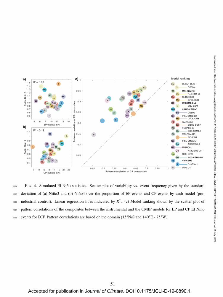
4 6 8 10 12 14 16EP events in %

0.50.60.70.80.9

11.11.21.31.41.5

Std

in N

iño

3

Aa

Ba

C

DEa

Fb

Ga I

Ka

L

Mb

NaOc

P

QcSb

UaB6

W6

E6

G6

I6

M6

Q6R6T6 O6

9 11 13 15 17 19 21 23CP events in %

0.4

0.5

0.6

0.7

0.8

0.9

1

1.1

Std

in N

iño

4

AaBa

C

DEa

Fb

Ga

I

Ka

L

Mb

Na

OcPQc

Sb Ua

B6W6

E6

G6

I6

M6

Q6R6

T6O6

0.65 0.7 0.75 0.8 0.85 0.9 0.95 1Pattern correlation of CP composites

0.65

0.7

0.75

0.8

0.85

0.9

0.95

1

Patte

rn c

orre

latio

n of

EP

com

posi

tes

Aa Ba

C

DEa

Fb

Ga

I

Ka

L

Mb

Na

Oc

P

Qc

Sb

Ua

B6

W6E6

G6

I6

M6

Q6

R6

T6

O6

R2 = 0.00

R2 = 0.19

a)

b)

c)

Aa ACCESS1-0

Ba BCC-CSM1-1

C BNU-ESM

D CCSM4Ea CESM1-BGC

Fb CMCC-CM

Ga CNRM-CM5

I CanESM2

Ka FGOALS-g2

L FIO-ESM

Mb GFDL-CM3

Na GISS-E2-HOc HadGEM2-CC

P INMCM4

Qc IPSL-CM5B-LR

Sb MPI-ESM-MR

B6 BCC-CSM2-MR

W6 CAMS-CSM1-0E6 CESM2

G6 CNRM-CM6-1

I6 CanESM5

M6 GFDL-CM4

Q6 IPSL-CM6A-LR

R6 MIROC6

T6 MRI-ESM2-0

O6 UKESM1-0-LL

Ua NorESM1-M

Model ranking

FIG. 4. Simulated El Nino statistics. Scatter plot of variability vs. event frequency given by the standard

deviation of (a) Nino3 and (b) Nino4 over the proportion of EP events and CP events by each model (pre-

industrial control). Linear regression fit is indicated by R2. (c) Model ranking shown by the scatter plot of

pattern correlations of the composites between the instrumental and the CMIP models for EP and CP El Nino

events for DJF. Pattern correlations are based on the domain (15◦N/S and 140◦E - 75◦W).

1024

1025

1026

1027

1028

51


Dow



-19-0890.1/4962286/jclid190890.pdf by UN

IVERSITY O

F TASMAN

IA MO

RR


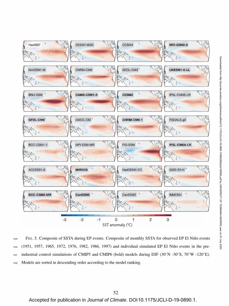
SST anomaly (°C)

FIG. 5. Composite of SSTA during EP events. Composite of monthly SSTA for observed EP El Nino events

(1951, 1957, 1965, 1972, 1976, 1982, 1986, 1997) and individual simulated EP El Nino events in the pre-

industrial control simulations of CMIP5 and CMIP6 (bold) models during DJF (30◦N -30◦S, 70◦W -120◦E).

Models are sorted in descending order according to the model ranking.

1029

1030

1031

1032

52


Dow



-19-0890.1/4962286/jclid190890.pdf by UN

IVERSITY O

F TASMAN

IA MO

RR


SST anomaly (°C)

FIG. 6. Composite of SSTA during CP events. Composite of monthly SSTA for observed CP El Nino events

(1963, 1968, 1977, 1979, 1987, 1991, 1994, 2002, 2004, 2009) and individual simulated CP El Nino events

in the pre-industrial control simulations of CMIP5 and CMIP6 (bold) models during DJF (30◦N -30◦S, 70◦W

-120◦E). Models are sorted in descending order according to the model ranking.

1033

1034

1035

1036

53


Dow



-19-0890.1/4962286/jclid190890.pdf by UN

IVERSITY O

F TASMAN

IA MO

RR


CESM

1-BG

CCC

SM4

MRI

-ESM

2-0

NorE

SM1-

MCN

RM-C

M5

GFDL

-CM

3UK

ESM

1-0-

LLBN

U-ES

MCA

MS-

CSM

1-0

CESM

2IP

SL-C

M5B

-LR

GFDL

-CM

4CM

CC-C

MCN

RM-C

M6-

1FG

OALS

-g2

BCC-

CSM

1-1

MPI

-ESM

-MR

FIO-

ESM

IPSL

-CM

6A-L

RAC

CESS

1-0

MIR

OC6

HadG

EM2-

CCGI

SS-E

2-H

BCC-

CSM

2-M

RCa

nESM

5Ca

nESM

2IN

MCM

4

0

5

10

15

EP e

vent

s in

%

EP events in control

ReconInstru

Ea D T6 Ua Ga Mb O6 C W6 E6 Qc M6 Fb G6 Ka Ba Sb L Q6 Aa R6 Oc Na B6 I6 I P

CESM

1-BG

CCC

SM4

MRI

-ESM

2-0

NorE

SM1-

MCN

RM-C

M5

GFDL

-CM

3UK

ESM

1-0-

LLBN

U-ES

MCA

MS-

CSM

1-0

CESM

2IP

SL-C

M5B

-LR

GFDL

-CM

4CM

CC-C

MCN

RM-C

M6-

1FG

OALS

-g2

BCC-

CSM

1-1

MPI

-ESM

-MR

FIO-

ESM

IPSL

-CM

6A-L

RAC

CESS

1-0

MIR

OC6

HadG

EM2-

CCGI

SS-E

2-H

BCC-

CSM

2-M

RCa

nESM

5Ca

nESM

2IN

MCM

4

0

5

10

15

20

CP

even

ts in

%

CP events in control

ReconInstru


b

CESM

1-BG

CCC

SM4

MRI

-ESM

2-0

NorE

SM1-

MCN

RM-C

M5

GFDL

-CM

3UK

ESM

1-0-

LLBN

U-ES

MCA

MS-

CSM

1-0

CESM

2IP

SL-C

M5B

-LR

GFDL

-CM

4CM

CC-C

MCN

RM-C

M6-

1FG

OALS

-g2

BCC-

CSM

1-1

MPI

-ESM

-MR

FIO-

ESM

IPSL

-CM

6A-L

RAC

CESS

1-0

MIR

OC6

HadG

EM2-

CCGI

SS-E

2-H

BCC-

CSM

2-M

RCa

nESM

5Ca

nESM

2IN

MCM

4

-10

-5

0

5

10

15

Cha

nges

rela

tive

to c

ontr

ol s

imul

atio

n in

%

RCP8.5/SSP585ca

EP El NiñoCP El Niño

0.3 0.4 0.5 0.6 0.7 0.8Global temperature change (°C/10yr)

-10

-5

0

5

10

15

Cha

nges

rela

tive

to c

ontr

ol s

imul

atio

n in

%

RCP8.5/SSP585

Ea

Ea

D

DT6

T6

Ua

Ua

GaGa

Mb

Mb

O6

O6

C

C

W6

W6

E6

E6

Qc

Qc

M6

M6

Fb

Fb

G6

G6

Ka

Ka

BaBa

Sb

Sb

L

L

Q6

Q6

Aa

Aa

R6

R6

Oc

Oc

Na

Na

B6B6

I6

I6

I

I

P

P

d


FIG. 7. Occurrence of different El Nino events and changes relative to pre-industrial control. Number of

EP (a) and CP (b) El Nino events given as % of all years in pre-industrial control simulations. Horizontal

lines show the number of events in the instrumental record (1870-1980:solid) and the reconstruction (1617-

1980:dashed).(c) Stacked changes are given as differences in % relative to the pre-industrial control simulation,

so that positive/negative deviations indicate more events/fewer events in the future emissions scenario. Change

values are derived from the RCP-8.5/SSP5-8.5 scenario. (d) Change values are also shown as a function of the

global mean temperature change in the RCP-8.5/SSP5-8.5 scenario (not significant at p < 0.05). Models are

ranked from best (left) to worst (right).

1037

1038

1039

1040

1041

1042

1043

1044

54


Dow



-19-0890.1/4962286/jclid190890.pdf by UN

IVERSITY O

F TASMAN

IA MO

RR


Range in control simulations Mean state change ZSG Trend

0.5

1

1.5

0.5

1

1.5

2

Recon

0.5

1

1.5

2

2.5

3

3.5

4

PII6B6NaOcR6AaQ6LSbBaKaG6FbM6QcE6W6CO6MbGaUaT6DEa



CES

M1-

BGC

CC

SM4

MR

I-ESM

2-0

Nor

ESM

1-M

CN

RM

-CM

5G

FDL-

CM

3U

KES

M1-

0-LL

BNU

-ESM

CA

MS-

CSM

1-0

CES

M2

IPSL

-CM

5B-L

RG

FDL-

CM

4C

MC

C-C

MC

NR

M-C

M6-

1FG

OAL

S-g2

BCC

-CSM

1-1

MPI

-ESM

-MR

FIO

-ESM

IPSL

-CM

6A-L

RAC

CES

S1-0

MIR

OC

6H

adG

EM2-

CC

GIS

S-E2

-HB

CC

-CSM

2-M

RC

anES

M5

Can

ESM

2IN

MC

M4

Aa

Ba

CDEaFb

Ga

I

Ka

L

Mb NaOc

P

Qc

Sb

Ua

B6

W6

E6

G6

I6M6

Q6

R6

T6

O6

La Niñalike

El Niñolike

Aa

BaC D

Ea

Fb

Ga

I

Ka

LMb

NaOcP

Qc

Sb

Ua

B6W6

E6

G6

I6M6Q6

R6

T6

O6

La Niñalike

El Niñolike

RCP8.5/SSP585

Aa

BaC D

EaFbGa

I

Ka

L

MbNaOc

P

Qc

Sb

Ua

B6

W6

E6

G6

I6M6

Q6

R6

T6

O6

La Niñalike

El Niñolike

Aa

Ba

CDEa

Fb

Ga

I

Ka

L

Mb NaOc

P

Qc

Sb

Ua

B6

W6

E6

G6

I6M6

Q6

R6

T6

O6

Aa

BaC D

Ea

Fb

Ga

I

Ka

LMb

NaOc

P

Qc

Sb

Ua

B6W6

E6

G6

I6 M6Q6

R6

T6

O6

-1 0 1 2 310-5

Aa

BaC D

EaFbGa

I

Ka

LMb

Na Oc

P

Qc

Sb

Ua

B6

W6

E6

G6

I6M6

Q6

R6

T6

O6

ZSG slope (RCP8.5/SSP585)

b)

a)

c)

d)

e)

f )

g)

h)

i)

j)

k)

l)

Num

ber o

f CP

El N

iño

even

ts

rela

tive

to a

vg. (

ref.

perio

d)N

umbe

r of E

P El

Niñ

o ev

ents

re

lativ

e to

avg

. (re

f. pe

riod)

Num

ber o

f CP/

EP E

l Niñ

o ev

ents

re

lativ

e to

avg

. (re

f. pe

riod)

Incr

ease

Dec

reas

eIn

crea

seD

ecre

ase

Incr

ease

Dec

reas

e

FIG. 8. Deviation changes of El Nino. Number of CP (a) and EP events (b) and the ratio of CP to EP events (c)

expressed by the average conditions divided by the mean of each reference period, so that the deviations larger

than 1 equal an increase/decrease relative to the reference mean. Left box plot: Recent observations (1980-

2016: red dot) relative to reconstructed variability derived from sliding window of 94 years relative to average

reference period (1617-1980)(a,b,c). Middle box plot: event variability in pre-industrial control simulations

derived from sliding window of 94 years relative to its mean (d,e,f). Right box plot: Average conditions in the

RCP-8.5/SSP5-8.5 scenario relative to the average pre-industrial control simulations for all models (boxplot)

and distinguished by models with a La Nina-like warming trend and El Nino-like warming trend derived from

the ZSG slope during the RCP-8.5/SSP5-8.5 period (g,h,i). Right plot: Changes relative to the pre-industrial

control simulations for individual models as a function of its ZSG slope in RCP-8.5/SSP5-8.5 (j,k,l). Regression

lines are separated for El Nino and La Nina-like warming models.

1045

1046

1047

1048

1049

1050

1051

1052

1053

1054

1055

55


Dow



-19-0890.1/4962286/jclid190890.pdf by UN

IVERSITY O

F TASMAN

IA MO

RR


Mb Q6 W6 G6 Ua C Ea Qc Aa L Oc Na D Fb Ga M6 Ba I6 R6 B6 O6 Ka E6 I P Sb T6

-0.05

0

0.05


-0.05

0

0.05


GFD

L-CM

3IP

SL-C

M6A

-LR

CAM

S-CS

M1-

0CN

RM-C

M6-

1No

rESM

1-M

BNU-

ESM

CESM

1-BG

CIP

SL-C

M5B

-LR

ACCE

SS1-

0FI

O-E

SMHa

dGEM

2-CC

GIS

S-E2

-HCC

SM4

CMCC

-CM

CNRM

-CM

5G

FDL-

CM4

BCC-

CSM

1-1

CanE

SM5

MIR

OC6

BCC-

CSM

2-M

RUK

ESM

1-0-

LLFG

OAL

S-g2

CESM

2Ca

nESM

2IN

MCM

4M

PI-E

SM-M

RM

RI-E

SM2-

0Ha

dISS

T

-0.05

0

0.05

Future decrease CP/EP activity Future increase CP/EP activity

zonal SST trend

CP frequency

EP frequency

CP/EP

Positive PDV(+)

Negative PDV(-)

Positive PDV(+)

Negative PDV(-)

Positive PDV(+)

Negative PDV(-)

Positive PDV(+)

Negative PDV(-)

Overall changes

Event frequency during PDV phases

Changes of event frequency duringPDV phases

CP El Niño

CP El Niño

EP El Niño

EP El Niño

a)

b)

c)

5·10-2

100

5·10-1

5·10-1

FIG. 9. Changes of El Nino frequencies and PDV phases. a, Summary of the zonal SST trend in the future

simulations (positive/negative: El Nino/La Nina-like warming pattern) and changes of event frequency of CP

events, EP events and the overall ratio of CP/EP events as the difference between RCP-8.5/SSP5-8.5 and pre-

industrial control simulations for 27 CMIP models and the early (1870-1980) and late (1981-2016) instrumental

HadISST record. CMIP5 and CMIP6 (bold) models are sorted according to their CP/EP ratio (4th row). b,

Difference of event frequency of CP and EP El Nino events during positive PDV and negative PDV periods

in the pre-industrial control simulations, relative to the individual model event frequency derived from the pre-

industrial control simulations and the entire instrumental HadISST record (1870-2016). c, Difference between

the event frequency of CP and EP events during PDV positive and PDV negative periods derived from the

pre-industrial control simulations and the RCP-8.5/SSP5-8.5 simulations.

1056

1057

1058

1059

1060

1061

1062

1063

1064

1065

56


Dow



-19-0890.1/4962286/jclid190890.pdf by UN

IVERSITY O

F TASMAN

IA MO

RR


CP El Niño

EP El Niño

Variability in control simulations

Variability in control simulations

Mean state change

Mean state change

Recon0

0.5

1

1.5

2

2.5

Recon

0.5

1

1.5

2

0

0.5

1

1.5

2

2.5


CES

M1-

BGC

CC

SM4

MR

I-ESM

2-0

Nor

ESM

1-M

CN

RM

-CM

5

GFD

L-C

M3

UK

ESM

1-0-

LL

BNU

-ESM

CA

MS-

CSM

1-0

CES

M2

IPSL

-CM

5B-L

R

GFD

L-C

M4

CM

CC

-CM

CN

RM

-CM

6-1

FGO

ALS-

g2

BCC

-CSM

1-1

MPI

-ESM

-MR

FIO

-ESM

IPSL

-CM

6A-L

R

ACC

ESS1

-0

MIR

OC

6

Had

GEM

2-C

C

GIS

S-E2

-H

BC

C-C

SM2-

MR

Can

ESM

5

Can

ESM

2

INM

CM

4

0.5

1

1.5

2


Aa

BaC D

EaFbGaI

KaL

Mb

NaOcPQc

SbUaB6W6E6

G6

I6M6

Q6R6

T6O6

La Niñalike

El Niñolike

RCP8.5/SSP585

AaBa

C

DEa

Fb

Ga

I

KaLMbNaOc

P

Qc

SbUaB6

W6

E6

G6I6M6

Q6

R6

T6

O6

La Niñalike

El Niñolike

Ea D T6 Ua Ga

Mb

O6 C

W6 E6 Qc

M6 Fb G6 Ka Ba Sb L

Q6 Aa R6 Oc

Na B6 I6 I P

Positive PDV(+)

Negative PDV(-)

Ea D T6 Ua Ga

Mb

O6 C

W6 E6 Qc

M6 Fb G6 Ka Ba Sb L

Q6 Aa R6 Oc

Na B6 I6 I P

Na Ea W6 Fb I6 E6 P Ga C I

Oc Qc T6 B6 Mb M6 D Ba O6 Q6 Sb Ua Ka Aa R6 L G6

-0.5

0

0.5

D L UaI

Ea O6 P B6 Mb Ka Oc Ba Q6 Sb I6 Na Ga Aa C G6 M6 R6 W6 Qc E6 Fb T6

-0.5

0

0.5

RCP8.5/SSP585C

ESM

1-BG

C

CC

SM4

MR

I-ESM

2-0

Nor

ESM

1-M

CN

RM

-CM

5

GFD

L-C

M3

UK

ESM

1-0-

LL

BNU

-ESM

CA

MS-

CSM

1-0

CES

M2

IPSL

-CM

5B-L

R

GFD

L-C

M4

CM

CC

-CM

CN

RM

-CM

6-1

FGO

ALS-

g2

BCC

-CSM

1-1

MPI

-ESM

-MR

FIO

-ESM

IPSL

-CM

6A-L

R

ACC

ESS1

-0

MIR

OC

6

Had

GEM

2-C

C

GIS

S-E2

-H

BC

C-C

SM2-

MR

Can

ESM

5

Can

ESM

2

INM

CM

4

a) b) c)

d)

f )g) h)

i)

j)

Future decrease CP intensity Future increase CP intensity

Future decrease EP intensity Future increase EP intensity

0

0.5

1

1.5

2

2.5

0.5

1

1.5

2

Positive PDV(+)

Negative PDV(-)

-0.5

0

0.5Positive PDV(+)

Negative PDV(-)

-0.5

0

0.5Positive PDV(+)

Negative PDV(-)

e)

FIG. 10. El Nino intensity of CP El Nino events (a-e) and EP El Nino events (f-j) derived from the recon-

structed 400 year reference period prior to 1980 (boxplot) and recent observation (red dot) (a,e), and from CMIP5

and CMIP6 (bold) pre-industrial control simulations (b,g) relative to different reference periods. Average CP (c)

and EP (h) El Nino intensity in the RCP-8.5/SSP5-8.5 scenario grouped by models with a La Nina-like warming

trend and El Nino-like warming trend (d,i). Difference of El Nino intensity during positive and negative PDV pe-

riods in the control simulations, relative to the individual model event frequency derived from the pre-industrial

control simulations (e,j) sorted according to the model ranking. Changes of El Nino intensity as the difference

of El Nino intensity during positive and negative PDV phases derived from the pre-industrial control simulations

and the RCP-8.5/SSP8-5.8 simulations (e,j), sorted from strongest declines (left) to largest increases (right) in

terms overall change.

1066

1067

1068

1069

1070

1071

1072

1073

1074

1075

57


Dow



-19-0890.1/4962286/jclid190890.pdf by UN

IVERSITY O

F TASMAN

IA MO

RR


HadIS

STAC

CESS

1-0

ACCE

SS1-

3

BCC-

CSM1-

1-M

BCC-

CSM1-

1BN

U-ES

MCC

SM4

CESM

1-BG

C

CESM

1-CA

M5

CESM

1-FA

STCH

EM

CESM

1-W

ACCM

CMCC

-CMS

CMCC

-CM

CNRM

-CM5

CSIR

O-Mk3

-6-0

CSIR

O-Mk3

L-1-

2Ca

nESM

2FG

OALS-

g2FG

OALS-

s2FI

O-ESM

GFDL-

CM3

GFDL-

ESM2G

GFDL-

ESM2M

GISS-

E2-H

GISS-

E2-R

GISS-

E2-R

GISS-

E2-R

HadG

EM2-

CCHa

dGEM

2-ES

INMCM

4

IPSL

-CM5A

-LR

IPSL

-CM5A

-MR

IPSL

-CM5B

-LR

MIROC-

ESM

MIROC4

hMIR

OC5MPI

-ESM

-LR

MPI-E

SM-M

RMPI

-ESM

-PMRI

-CGCM

3No

rESM

1-ME

NorE

SM1-

M

BCC-

CSM2-

MR

CAMS-

CSM1-

0CE

SM2

CNRM

-CM6-

1Ca

nESM

5GFD

L-CM

4

IPSL

-CM6A

-LR

MIROC6

MRI-E

SM2-

0

UKES

M1-0-

LL

0.5

1

1.5

2

2.5

SSTA

Std

Dev

(DJF

/AM

J) Obs CMIP6CMIP5

Aa

AbBb

BaC D Ea Eb

Ed EeFc

FbGa

HaHb

I

Ka

Kb

LMb

McMd Na

Nc Nc Nc Oc Od

P QaQbQc Ra

Rc

Rd Sa Sb Sc

TaUb Ua

B6W6E6 G6

I6

M6

Q6 R6 T6O6

HadIS

STAC

CESS

1-0

ACCE

SS1-

3

BCC-

CSM1-

1-M

BCC-

CSM1-

1BN

U-ES

MCC

SM4

CESM

1-BG

C

CESM

1-CA

M5

CESM

1-FA

STCH

EM

CESM

1-W

ACCM

CMCC

-CMS

CMCC

-CM

CNRM

-CM5

CSIR

O-Mk3

-6-0

CSIR

O-Mk3

L-1-

2Ca

nESM

2FG

OALS-

g2FG

OALS-

s2FI

O-ESM

GFDL-

CM3

GFDL-

ESM2G

GFDL-

ESM2M

GISS-

E2-H

GISS-

E2-R

GISS-

E2-R

GISS-

E2-R

HadG

EM2-

CCHa

dGEM

2-ES

INMCM

4

IPSL

-CM5A

-LR

IPSL

-CM5A

-MR

IPSL

-CM5B

-LR

MIROC-

ESM

MIROC4

hMIR

OC5MPI

-ESM

-LR

MPI-E

SM-M

RMPI

-ESM

-PMRI

-CGCM

3No

rESM

1-ME

NorE

SM1-

M

BCC-

CSM2-

MR

CAMS-

CSM1-

0CE

SM2

CNRM

-CM6-

1Ca

nESM

5GFD

L-CM

4

IPSL

-CM6A

-LR

MIROC6

MRI-E

SM2-

0

UKES

M1-0-

LL

0.5

1

1.5

2

2.5

SSTA

Std

Dev

(DJF

/AM

J) Obs CMIP6CMIP5

Aa

Ab

Bb Ba

CD Ea

EbEd

Ee

Fc Fb

Ga

Ha

Hb

IKa

Kb

L MbMcMd

NaNc

Nc

Nc

Oc Od P

Qa Qb

Qc RaRc

Rd Sa Sb Sc Ta

Ub Ua B6W6E6

G6I6

M6

Q6R6 T6

O6

(a)

(b)

Fig. A1. Seasonal phase locking. Phase locking index (PLI) based on the Nino4 index (a) and Nino3 index

(b) for all CMIP5 and CMIP6 models compared to the observed (HadISST: dashed line).

1076

1077

58


Dow



-19-0890.1/4962286/jclid190890.pdf by UN

IVERSITY O

F TASMAN

IA MO

RR


1880 1900 1920 1940 1960 1980 2000 2020

-0.8

-0.6

-0.4

-0.2

0

0.2

0.4

0.6

0.8

0.1818 0.0909 0.1935 0.23810.0909 0.2727 0.0968 0.0952

0.1250 0.0 0.0 0.0476 0.2727 0.31250.1250 0.1250 0.0 0.0952 0.1818 0.0

Positive PDV phasePDV(+)

NegativePDV

phasePDV(-)

EP El Niño eventsCP El Niño events

Event frequency during PDV negative phase:

EP frequencyCP frequency

EP frequencyCP frequency

Event frequency during PDV positive phase:

TPI index

Fig. A2. Occurrence of different types of El Nino. Observed occurrence of EP and CP El Nino events

according to Freund et al. (2019) during the instrumental period (1870-2018). Insets show the event occurrence

frequencies during PDV positive phases (upper inset) and PDV positive phases (lower inset) based on shaded

observed periods of PDV based on TPI index (Henley et al. 2015).

1078

1079

1080

1081

59


Dow



-19-0890.1/4962286/jclid190890.pdf by UN

IVERSITY O

F TASMAN

IA MO

RR


EP events

10 20 30 40 50 60Window size (years)

ACCESS1-0BCC-CSM1-1

BNU-ESMCCSM4

CESM1-BGCCMCC-CM

CNRM-CM5CanESM2

FGOALS-g2FIO-ESM

GFDL-CM3GISS-E2-H

HadGEM2-CCINMCM4

IPSL-CM5B-LRMPI-ESM-MR

NorESM1-MBCC-CSM2-MRCAMS-CSM1-0

CESM2CNRM-CM6-1

CanESM5GFDL-CM4

IPSL-CM6A-LRMIROC6


CP events


ACCESS1-0BCC-CSM1-1

BNU-ESMCCSM4

CESM1-BGCCMCC-CM

CNRM-CM5CanESM2

FGOALS-g2FIO-ESM

GFDL-CM3GISS-E2-H

HadGEM2-CCINMCM4



CESM2CNRM-CM6-1

CanESM5GFDL-CM4

IPSL-CM6A-LRMIROC6

MRI-ESM2-0UKESM1-0-LL 30

40

50

60

70

80

90

100

Agre

emen

t in

%

EP events


ACCESS1-0BCC-CSM1-1

BNU-ESMCCSM4

CESM1-BGCCMCC-CM

CNRM-CM5CanESM2

FGOALS-g2FIO-ESM

GFDL-CM3GISS-E2-H

HadGEM2-CCINMCM4



CESM2CNRM-CM6-1

CanESM5GFDL-CM4

IPSL-CM6A-LRMIROC6


CP events


ACCESS1-0BCC-CSM1-1

BNU-ESMCCSM4

CESM1-BGCCMCC-CM

CNRM-CM5CanESM2

FGOALS-g2FIO-ESM

GFDL-CM3GISS-E2-H

HadGEM2-CCINMCM4



CESM2CNRM-CM6-1

CanESM5GFDL-CM4

IPSL-CM6A-LRMIROC6

MRI-ESM2-0UKESM1-0-LL 30

40

50

60

70

80

90

100

Agre

emen

t in

%

(a)

(b)

Fig. A3. Sensitivity to normalization period/window approach. Comparison of the EP El Nino (left) and

CP El Nino (right) event detection for different normalization windows for pre-industrial control simulations

(a) and RCP-8.5/SSP5-8.5 scenario simulations (b). Shown is the agreement in % of El Nino events that have

been identified using different window sizes (x-axis) relative to the El Nino events identified using the 30-year

window size.

1082

1083

1084

1085

1086

60


Dow



-19-0890.1/4962286/jclid190890.pdf by UN

IVERSITY O

F TASMAN

IA MO

RR


Documents

Warming patterns affect El Nino diversity in CMIP5 …...1 Warming patterns affect El Nino diversity in CMIP5 and CMIP6 models˜ Mandy B. Freund 2 CSIRO Agriculture and Food, Melbourne,