Embed Size (px)
Citation preview
Prepared for submission to JHEP JLAB-THY-18-2775
Semi-Inclusive Deep-Inelastic Scattering inWandzura–Wilczek-type approximation
S. Bastamia H. Avakianb A. V. Efremovc A. Kotziniand,e B. U. Muschf
B. Parsamyank A. Prokuding,b M. Schlegelh G. Schnelli P. Schweitzera,j K. Tezgina
aDepartment of Physics, University of Connecticut, Storrs, CT 06269, U.S.A.bThomas Jefferson National Accelerator Facility, Newport News, VA 23606, U.S.A.cJoint Institute for Nuclear Research, Dubna, 141980 RussiadYerevan Physics Institute, Alikhanyan Brothers St., 375036 Yerevan, ArmeniaeINFN, Sezione di Torino, 10125 Torino, Italyf Institut für Theoretische Physik, Universität Regensburg, 93040 Regensburg, GermanygDivision of Science, Penn State Berks, Reading, PA 19610, USAkCERN, 1211 Geneva 23, SwitzerlandhDepartment of Physics, New Mexico State University, Las Cruces, NM 88003-001, USAiDepartment of Theoretical Physics, University of the Basque Country UPV/EHU, 48080 Bilbao,Spain, and IKERBASQUE, Basque Foundation for Science, 48013 Bilbao, SpainjInstitute for Theoretical Physics, Universität Tübingen, D-72076 Tübingen, Germany
E-mail: [email protected], [email protected],[email protected], [email protected], [email protected],[email protected], [email protected], [email protected],[email protected], [email protected],[email protected]
Abstract: We present the complete cross-section for the production of unpolarizedhadrons in semi-inclusive deep-inelastic scattering up to power-suppressed O(1/Q2) termsin the Wandzura–Wilczek-type approximation, which consists in systematically assumingthat qgq–terms are much smaller than qq–correlators. We compute all twist-2 and twist-3structure functions and the corresponding asymmetries, and discuss the applicability of theWandzura–Wilczek-type approximations on the basis of available data. We make predic-tions that can be tested by data from COMPASS, HERMES, Jefferson Lab, and the futureElectron-Ion Collider. The results of this paper can be readily used for phenomenology andfor event generators, and will help to improve the description of semi-inclusive deep-inelasticprocesses in terms of transverse momentum dependent parton distribution functions andfragmentation functions beyond the leading twist.
Keywords: Wandzura–Wilczek approximation, semi-inclusive deep-inelastic scattering,transverse momentum dependent distribution and fragmentation functions, spin and az-imuthal asymmetries, leading and subleading twist
arX
iv:1
807.
1060
6v2
[he
p-ph
] 1
4 Ja
n 20
19
Contents
1 Introduction 2
2 The SIDIS process in terms of TMDs and FFs 42.1 The SIDIS process 42.2 TMDs, FFs and structure functions 7
3 WW and WW-type approximations 113.1 WW approximation for PDFs 123.2 WW-type approximations for TMDs and FFs 123.3 Predictions from instanton vacuum model 143.4 Tests of WW approximation in DIS experiments 153.5 Tests in lattice QCD 163.6 Tests in models 193.7 Basis functions for the WW-type approximations 203.8 Limitation of WW-type approximations 20
4 SIDIS in the WW-type approximation and Gaussian model 224.1 Leading structure functions amenable to WW-type approximations 224.2 Subleading structure functions in WW-type approximations 224.3 Gaussian Ansatz for TMDs and FFs 234.4 Evaluation of structure functions in WW-type & Gaussian approximation 234.5 Phenomenological information on basis functions 24
5 Leading-twist asymmetries and basis functions 265.1 Leading-twist FUU and Gaussian Ansatz 265.2 Leading-twist ALL and first test of Gaussian Ansatz in polarized scattering 285.3 Leading-twist Asin(φh−φS)
UT Sivers asymmetry 295.4 Leading-twist Asin(φh+φS)
UT Collins asymmetry 305.5 Leading-twist Acos(2φh)
UU Boer–Mulders asymmetry 315.6 Leading-twist Asin(3φh−φS)
UT asymmetry 325.7 Statistical and systematic uncertainties of basis functions 33
6 Leading-twist asymmetries in WW-type approximation 336.1 Leading-twist Acos(φh−φS)
LT 346.2 Leading-twist Asin 2φh
UL Kotzinian–Mulders asymmetry 346.3 Inequalities and a cross check 36
– i –
7 Subleading-twist asymmetries in WW-type approximation 377.1 Subleading-twist Asinφh
LU 377.2 Subleading-twist AcosφS
LT 387.3 Subleading-twist Acos(2φh−φS)
LT 397.4 Subleading-twist Acosφh
LL 417.5 Subleading-twist Asinφh
UL 417.6 Subleading-twist AsinφS
UT 437.7 Subleading-twist Asin(2φh−φS)
UT 447.8 Subleading-twist Acosφh
UU 44
8 Conclusions 46
9 Acknowledgments 48
A The “minimal basis” of TMDs and FFs 48A.1 Unpolarized functions fa1 (x, k
2⊥) and Da
1(z, P2⊥) 48
A.2 Helicity distribution ga1(x, k2⊥) 49
A.3 Sivers function f⊥q1T (x, k⊥) 50A.4 Transversity hq1(x, k⊥) and Collins function H⊥q1 (x, P⊥) 51A.5 Boer-Mulders function h⊥q1 (x, k⊥) 52A.6 Pretzelosity distribution h⊥q1T (x, k⊥) 53
B Convolution integrals and expressions in Gaussian Ansatz 53B.1 Notation for convolution integrals 53B.2 Gaussian Ansatz 54B.3 Gaussian Ansatz for the derived TMDs used in this work 54B.4 Comment on TMDs subject to the sum rules (2.14) 55B.5 Convolution integrals in Gaussian Ansatz 56
C Mathematica package 57
– 1 –
1 Introduction
A great deal of what is known about the quark-gluon structure of nucleons is due to studiesof parton distribution functions (PDFs) in deep-inelastic reactions. Leading-twist PDFs tellus how likely it is to find an unpolarized parton [described by PDF fa1 (x), a = q, q, g] ora longitudinally polarized parton [described by PDF ga1(x), a = q, q, g] in a fast-movingunpolarized or longitudinally polarized nucleon, which carries the fraction x of the nucleonmomentum. This information depends on the “resolution (renormalization) scale” associ-ated with the hard scale Q of the process. Although the PDFs fa1 (x) and ga1(x) continuebeing the subject of intense research (small-x, large-x, helicity sea and gluon distributions)they can be considered as rather well known, and the frontier has been extended in the lastyears to go beyond the one-dimensional picture offered by those PDFs.
One way to do this consists in a systematic inclusion of transverse parton momenta k⊥,whose effects manifest themselves in terms of transverse momenta of the reaction productsin the final state. If these transverse momenta are much smaller than the hard scale Q of theprocess, the formal description is given in terms of transverse momentum dependent distri-bution functions (TMDs) and fragmentation functions (FFs), which are defined in terms ofquark-quark correlators [1–5]. Both of them depend on two independent variables: in thecase of TMDs, on the fraction x of nucleon momentum carried by the parton and intrinsictransverse momentum k⊥ of the parton, while in the case of FFs, on the fraction z of theparton momentum transferred to the hadron and the transverse momentum of the hadronacquired during the fragmentation process. Being a vector in the plane transverse withrespect to the light-cone direction singled out by the hard-momentum flow in the process,k⊥ allows us to access novel information on the nucleon spin structure through correla-tions of k⊥ with the nucleon and/or parton spin. The latter is a well-defined concept fortwist-2 TMDs interpreted in the infinite momentum frame or in the lightcone quantizationformalism.
One powerful tool to study TMDs are measurements of the semi-inclusive deep-inelasticscattering (SIDIS) process. By exploring various possibilities for the lepton beam and targetpolarizations unambiguous information can be accessed on the 8 leading-twist TMDs [3]and, if one assumes factorization, on certain linear combinations of the 16 subleading-twistTMDs [4, 5]. It is important to stress that this information could not have been obtainedwithout advances in target polarization techniques employed in the HERMES, COMPASSand Jefferson Lab (JLab) experiments [6–9]. Complementary information can be obtainedfrom the Drell–Yan process [10], and e+e− annihilation [11].
In QCD the TMDs are independent functions. Each TMD contains unique informationon a different aspect of the nucleon structure. Twist-2 TMDs have partonic interpretations.Twist-3 TMDs give insights on quark-gluon correlations in the nucleon [12–14]. Besidespositivity constraints [15] there is little model-independent information on TMDs. Animportant question with practical applications is: do useful approximations for TMDsexist? Experience from collinear PDFs encourages to explore this possibility: the twist-3gaT (x) and haL(x) can be respectively expressed in terms of contributions from twist-2 ga1(x)
and ha1(x), and additional quark-gluon-quark (qgq) correlations or current-quark mass terms
– 2 –
[16, 17] (the index a = q , q does not include gluons for ha1, haL and other chiral-odd TMDsbelow). We shall refer to the latter generically as qgq–terms, keeping in mind one deals ineach case with matrix elements of different operators. The qgq–correlations contain newinsights on hadron structure, which are worthwhile exploring for their own sake, see forinstance Ref. [18] on gaT (x).
The striking observation is that the qgq–terms in gaT (x) and haL(x) are small: theoreticalmechanisms predict this [19–22], and in the case of gaT (x) data confirm or are compatiblewith these predictions [23–25]. This approximation (“neglect of qgq–terms”) is commonlyknown as Wandzura–Wilczek (WW) approximation [16]. The possibility to apply this typeof approximation also to TMDs has been explored in specific cases in [26–32]. In both cases,PDFs and TMDs, one basically assumes that the contributions from qgq–terms can be ne-glected with respect to qq–terms. But the nature of the omitted matrix elements is different,and in the context of TMDs one often prefers to speak about WW-type approximations.
The present work is the first study of all SIDIS structure functions up to twist-3 in aunique approach. Our results are of importance for measurements performed or in prepa-ration at COMPASS, HERMES, and JLab with 12GeV beam-energy upgrade, or proposedin the long-term (Electron-Ion Collider), and provide helpful input for the development ofMonte Carlo event generators [33].
On the theoretical side it is also important to note that the theory for subleading-twistTMD observables is only poorly developed as compared to the current state-of-the-art ofleading-twist observables. In order to address subleading-twist TMD observables one hasto restrict oneself to the tree-level formalism [1–5], which may not be free of doubts [34, 35].
Our predictions, whether confirmed or not supported by current and future experimen-tal data, will in any case provide a useful benchmark, and call for dedicated theoreticalstudies to explain (i) why the pertinent qgq–terms are small or (ii) why they are sizable,depending on the outcome of the experiments. In either case our results will deepen theunderstanding of qgq–correlations, pave the way towards testing the validity of the TMDfactorization approach at subleading twist, and help us to guide further developments.
In this work, after introducing the SIDIS process and defining TMDs and FFs (Sec. 2),we shall introduce the WW(-type) approximations, and review what is presently knownabout them from experiment and theory (Sec. 3). We will show that under the assumptionof the validity of these approximations all leading and subleading SIDIS structure functionsare described in terms of a basis of 6 TMDs and 2 FFs (Sec. 4), and review how these basisfunctions describe available data (Sec. 5). We will systematically apply the WW and/orWW-type approximations to SIDIS structure functions at leading (Sec. 6) and subleading(Sec. 7) twist, and conclude with a critical discussion (Sec. 8). The Appendices A and Bcontain technical details. In App. C we describe an open-source package implemented inMathematica [36] (already available) and Python (to be released in the near future) that ismade publicly available on github.com: https://github.com/prokudin/WW-SIDIS
– 3 –
2 The SIDIS process in terms of TMDs and FFs
In this section we review the description of the SIDIS process, define structure functions,PDFs, TMDs, FFs and recall how they describe the SIDIS structure functions.
2.1 The SIDIS process
Θ
����������������������
����������������������
����������
����������
z−axis
hφS
φh
Ph
l’
l
q
HADRON PRODUCTION PLANE
LEPTON SCATTERING PLANE
N
S
S
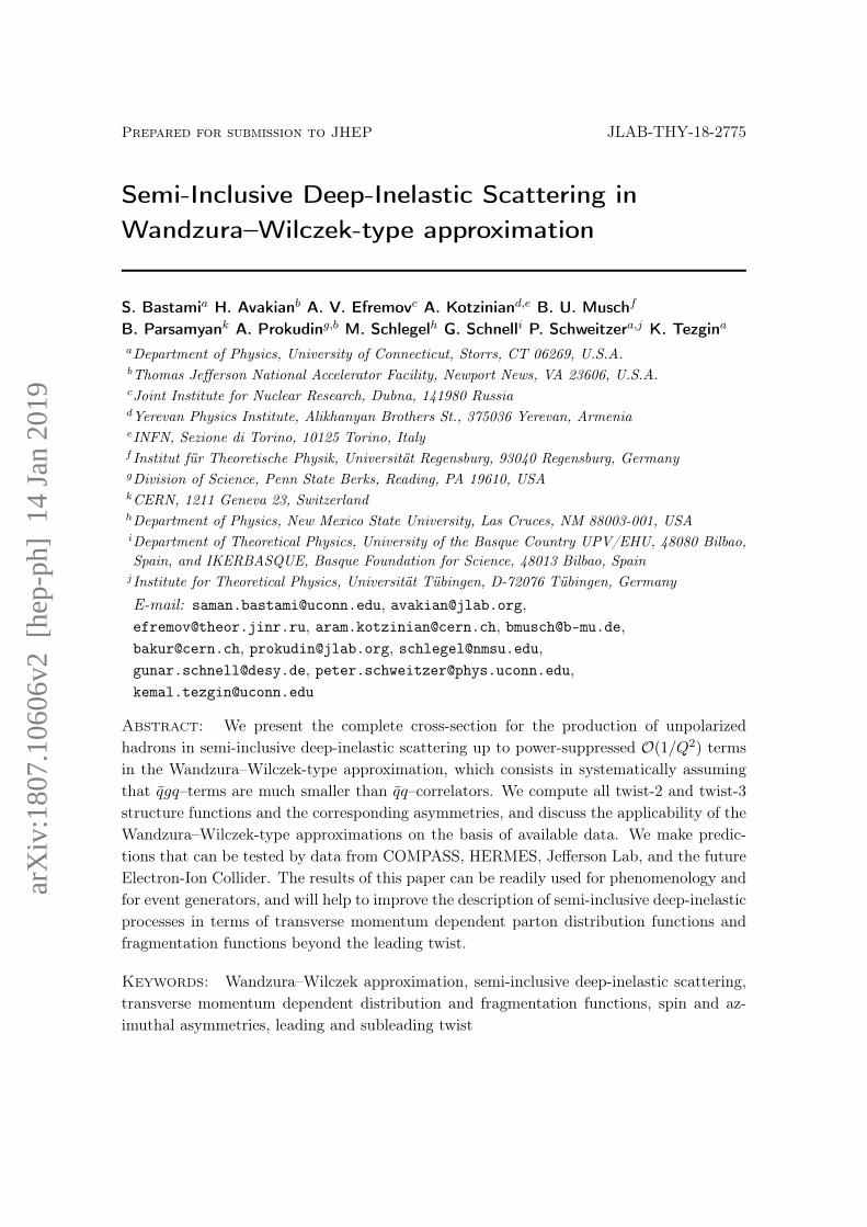
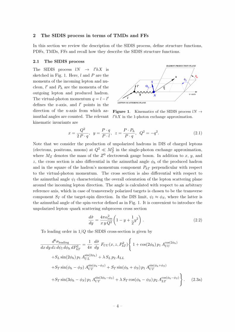
Figure 1. Kinematics of the SIDIS process lN →l′hX in the 1-photon exchange approximation.
The SIDIS process lN → l′hX issketched in Fig. 1. Here, l and P are themomenta of the incoming lepton and nu-cleon, l′ and Ph are the momenta of theoutgoing lepton and produced hadron.The virtual-photon momentum q = l− l′
defines the z-axis, and l′ points in thedirection of the x-axis from which az-imuthal angles are counted. The relevantkinematic invariants are
x =Q2
2P · q, y =
P · qP · l
, z =P · PhP · q
, Q2 = −q2. (2.1)
Note that we consider the production of unpolarized hadrons in DIS of charged leptons(electrons, positrons, muons) at Q2 � M2
Z in the single-photon exchange approximation,where MZ denotes the mass of the Z0 electroweak gauge boson. In addition to x, y, andz, the cross section is also differential in the azimuthal angle φh of the produced hadronand in the square of the hadron’s momentum component PhT perpendicular with respectto the virtual-photon momentum. The cross section is also differential with respect tothe azimuthal angle ψl characterizing the overall orientation of the lepton scattering planearound the incoming lepton direction. The angle is calculated with respect to an arbitraryreference axis, which in case of transversely polarized targets is chosen to be the transversecomponent ST of the target-spin direction. In the DIS limit, ψl ≈ φS , where the latter isthe azimuthal angle of the spin-vector defined as in Fig. 1. It is convenient to introduce theunpolarized lepton–quark scattering subprocess cross section
dσ
dy=
4πα2em
x y Q2
(1− y +
1
2y2
). (2.2)
To leading order in 1/Q the SIDIS cross-section is given by
d6σleading
dx dy dz dψl dφh dP2hT
=1
4π
dσ
dyFUU (x, z, P 2
hT )
{1 + cos(2φh) p1A
cos(2φh)UU
+SL sin(2φh) p1Asin(2φh)UL + λSL p2ALL
+ST sin(φh − φS)Asin(φh−φS)UT + ST sin(φh + φS) p1A
sin(φh+φS)UT
+ST sin(3φh − φS) p1Asin(3φh−φS)UT + λST cos(φh − φS) p2A
cos(φh−φS)LT
}. (2.3a)
– 4 –
Here FUU is the structure function due to transverse polarization of the virtual photon(sometimes denoted as FUU,T ), and we neglect 1/Q2 corrections in kinematic factors anda structure function (sometimes denoted as FUU,L) arising from longitudinal polarizationof the virtual photon (and another structure function ∝ ST sin(φh − φS), see below). Thestructure functions (and asymmetries) also depend on Q2 via the scale dependence of TMDsand FFs, which we do not show in formulas throughout this work.
At subleading order in the 1/Q expansion one has
d6σsubleading
dx dy dz dψl dφh dP2hT
=1
4π
dσ
dyFUU (x, z, P 2
hT )
{cos(φh) p3A
cos(φh)UU
+λ sin(φh) p4Asin(φh)LU + SL sin(φh) p3A
sin(φh)UL + λSL cos(φh) p4A
cos(φh)LL
+ST sin(2φh − φS) p3Asin(2φh−φS)UT + ST sin(φS) p3A
sin(φS)UT
+λST cos(φS) p4Acos(φS)LT + λST cos(2φh − φS) p4A
cos(2φh−φS)LT
}. (2.3b)
Neglecting 1/Q2 corrections, the kinematic prefactors pi are given by
p1 =1− y
1− y + 12 y
2, p2 =
y(1− 12 y)
1− y + 12 y
2, p3 =
(2− y)√
1− y1− y + 1
2 y2, p4 =
y√
1− y1− y + 1
2 y2,
(2.4)and the asymmetries Aweight
XY , are defined in terms of structure functions FweightXY , as follows
AweightXY ≡ Aweight
XY (x, z, PhT ) =FweightXY (x, z, PhT )
FUU (x, z, PhT ). (2.5)
Here, the first subscript X = U(L) denotes the unpolarized beam (longitudinally polarizedbeam with helicity λ). The second subscript Y = U(L or T ) refers to the target, which canbe unpolarized (longitudinally or transversely polarized with respect to the virtual photon).The superscript “weight” indicates the azimuthal dependence with no index indicating anisotropic angular distribution of the produced hadrons.
In the partonic description the structure functions in (2.3a) are “twist-2.” Those in(2.3b) are “twist-3” and contain a factor MN/Q in their definitions, see below, where MN
is the nucleon mass. In our treatment to 1/Q2 accuracy we neglect two structure functionsdue to longitudinal virtual-photon polarization, which contribute at order O(M2
N/Q2) in
the partonic description of the process, one being FUU,L and the other contributing to thesin(φh − φS) angular distribution [5].
Experimental collaborations often define asymmetries in terms of counts N(φh). Thismeans the kinematic prefactors pi and 1/(x y Q2) are included in the numerators or denom-inators of the asymmetries which are averaged over y within experimental kinematics. Wewill call the corresponding asymmetries Aweight
XY,〈y〉. For instance, in the unpolarized case onehas
N(x, . . . , φ) =N0(x, . . . )
2π
(1 + cosφ Acosφh
UU,〈y〉(x, . . . ) + cos 2φ Acos 2φhUU,〈y〉 (x, . . . )
)(2.6)
– 5 –
where N0 denotes the total (φh–averaged) number of counts and the dots indicate furtherkinematic variables in the kinematic bin of interest (which may also be averaged over). Itwould be preferable if asymmetries were analyzed with known kinematic prefactors dividedout on event-by-event basis. One could then directly compare asymmetries Aweight
XY mea-sured in different experiments and kinematics, and focus on effects of evolution or powersuppression for twist-3. In practice, often the kinematic factors were included. We willdefine and comment on the explicit expressions as needed.
For completeness we remark that after integrating the cross section over transversehadron momenta one obtains
d4σleading
dx dy dz dψl=
1
2π
dσ
dyFUU (x, z)
{1 + λSL p2ALL
}(2.7a)
d4σsubleading
dx dy dz dψl=
1
2π
dσ
dyFUU (x, z)
{ST sin(φS) p3A
sin(φS)UT + λST cos(φS) p4A
cos(φS)LT
},(2.7b)
where (and analogous for the other structure functions)
FUU (x, z) =
∫d2PhT FUU (x, z, PhT ) (2.8)
and the asymmetries are defined as
AweightXY (x, z) =
FweightXY (x, z)
FUU (x, z). (2.9)
The connection of “collinear” SIDIS structure functions in (2.7a, 2.7b) to those knownfrom inclusive DIS is established by integrating over z and summing over hadrons as
∑h
∫dz z FUU (x, z) ≡ 2xF1(x) , (2.10a)
∑h
∫dz z FLL(x, z) ≡ 2x g1(x) , (2.10b)
∑h
∫dz z F cosφS
LT (x, z) ≡ − γ 2x
(g1(x) + g2(x)
), (2.10c)
∑h
∫dz z F sinφS
UT (x, z) = 0 , (2.10d)
where γ = 2MNx/Q signals the twist-3 character of F cosφSLT (x, z). Notice that F sinφS
UT (x, z)
has no DIS counterpart due to time-reversal symmetry of strong interactions, and termssuppressed by 1/Q2 are consequently neglected throughout this work including the twist-4DIS structure function FL(x).
– 6 –
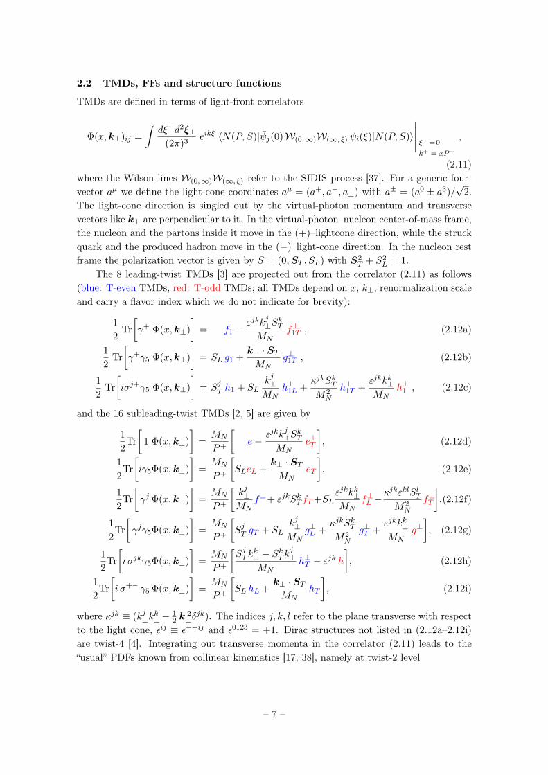
2.2 TMDs, FFs and structure functions
TMDs are defined in terms of light-front correlators
Φ(x,k⊥)ij =
∫dξ−d2ξ⊥
(2π)3eikξ 〈N(P, S)|ψj(0)W(0,∞)W(∞, ξ) ψi(ξ)|N(P, S)〉
∣∣∣∣∣ ξ+ =0
k+ = xP+
,
(2.11)where the Wilson lines W(0,∞)W(∞, ξ) refer to the SIDIS process [37]. For a generic four-vector aµ we define the light-cone coordinates aµ = (a+, a−, a⊥) with a± = (a0 ± a3)/
√2.
The light-cone direction is singled out by the virtual-photon momentum and transversevectors like k⊥ are perpendicular to it. In the virtual-photon–nucleon center-of-mass frame,the nucleon and the partons inside it move in the (+)–lightcone direction, while the struckquark and the produced hadron move in the (−)–light-cone direction. In the nucleon restframe the polarization vector is given by S = (0,ST , SL) with S2
T + S2L = 1.
The 8 leading-twist TMDs [3] are projected out from the correlator (2.11) as follows(blue: T-even TMDs, red: T-odd TMDs; all TMDs depend on x, k⊥, renormalization scaleand carry a flavor index which we do not indicate for brevity):
1
2Tr
[γ+ Φ(x,k⊥)
]= f1 −
εjkkj⊥SkT
MNf⊥1T , (2.12a)
1
2Tr
[γ+γ5 Φ(x,k⊥)
]= SL g1 +
k⊥ · STMN
g⊥1T , (2.12b)
1
2Tr
[iσj+γ5 Φ(x,k⊥)
]= SjT h1 + SL
kj⊥MN
h⊥1L +κjkSkTM2N
h⊥1T +εjkkk⊥MN
h⊥1 , (2.12c)
and the 16 subleading-twist TMDs [2, 5] are given by
1
2Tr
[1 Φ(x,k⊥)
]=MN
P+
[e−
εjkkj⊥SkT
MNe⊥T
], (2.12d)
1
2Tr
[iγ5Φ(x,k⊥)
]=MN
P+
[SLeL +
k⊥ · STMN
eT
], (2.12e)
1
2Tr
[γj Φ(x,k⊥)
]=MN
P+
[kj⊥MN
f⊥+ εjkSkT fT +SLεjkkk⊥MN
f⊥L −κjkεklSlTM2N
f⊥T
],(2.12f)
1
2Tr
[γjγ5Φ(x,k⊥)
]=MN
P+
[SjT gT + SL
kj⊥MN
g⊥L +κjkSkTM2N
g⊥T +εjkkk⊥MN
g⊥], (2.12g)
1
2Tr
[i σjkγ5Φ(x,k⊥)
]=MN
P+
[SjTk
k⊥ − SkTk
j⊥
MNh⊥T − εjk h
], (2.12h)
1
2Tr
[i σ+− γ5 Φ(x,k⊥)
]=MN
P+
[SL hL +
k⊥ · STMN
hT
], (2.12i)
where κjk ≡ (kj⊥kk⊥−
12 k
2⊥δ
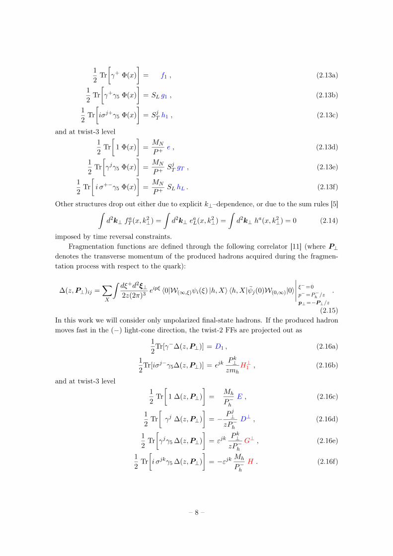
jk). The indices j, k, l refer to the plane transverse with respectto the light cone, εij ≡ ε−+ij and ε0123 = +1. Dirac structures not listed in (2.12a–2.12i)are twist-4 [4]. Integrating out transverse momenta in the correlator (2.11) leads to the“usual” PDFs known from collinear kinematics [17, 38], namely at twist-2 level
– 7 –
1
2Tr
[γ+ Φ(x)
]= f1 , (2.13a)
1
2Tr
[γ+γ5 Φ(x)
]= SL g1 , (2.13b)
1
2Tr
[iσj+γ5 Φ(x)
]= SjT h1 , (2.13c)
and at twist-3 level1
2Tr
[1 Φ(x)
]=MN
P+e , (2.13d)
1
2Tr
[γjγ5 Φ(x)
]=MN
P+SjT gT , (2.13e)
1
2Tr
[i σ+−γ5 Φ(x)
]=MN
P+SL hL . (2.13f)
Other structures drop out either due to explicit k⊥–dependence, or due to the sum rules [5]∫d2k⊥ f
aT (x, k2
⊥) =
∫d2k⊥ e
aL(x, k2
⊥) =
∫d2k⊥ h
a(x, k2⊥) = 0 (2.14)
imposed by time reversal constraints.Fragmentation functions are defined through the following correlator [11] (where P⊥
denotes the transverse momentum of the produced hadrons acquired during the fragmen-tation process with respect to the quark):
∆(z,P⊥)ij =∑X
∫dξ+d2ξ⊥2z(2π)3
eipξ 〈0|W(∞,ξ)ψi(ξ) |h,X〉 〈h,X|ψj(0)W(0,∞)|0〉
∣∣∣∣∣ ξ−=0
p−=P−h /z
p⊥=−P⊥/z
.
(2.15)In this work we will consider only unpolarized final-state hadrons. If the produced hadronmoves fast in the (−) light-cone direction, the twist-2 FFs are projected out as
1
2Tr[γ−∆(z,P⊥)] = D1 , (2.16a)
1
2Tr[iσj−γ5∆(z,P⊥)] = εjk
P k⊥zmh
H⊥1 , (2.16b)
and at twist-3 level1
2Tr
[1 ∆(z,P⊥)
]=
Mh
P−hE , (2.16c)
1
2Tr
[γj ∆(z,P⊥)
]= −
P j⊥zP−h
D⊥ , (2.16d)
1
2Tr
[γjγ5 ∆(z,P⊥)
]= εjk
P k⊥zP−h
G⊥ , (2.16e)
1
2Tr
[i σjkγ5 ∆(z,P⊥)
]= −εjk Mh
P−hH . (2.16f)
– 8 –
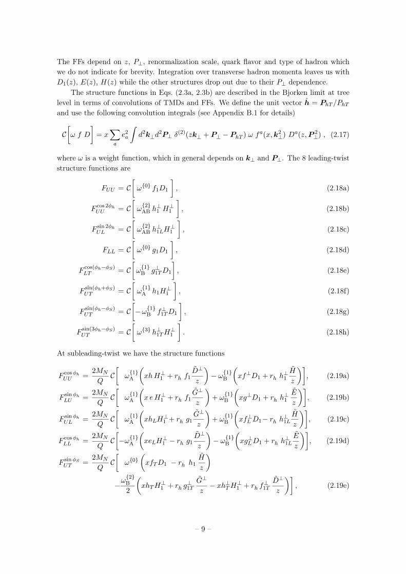
The FFs depend on z, P⊥, renormalization scale, quark flavor and type of hadron whichwe do not indicate for brevity. Integration over transverse hadron momenta leaves us withD1(z), E(z), H(z) while the other structures drop out due to their P⊥ dependence.
The structure functions in Eqs. (2.3a, 2.3b) are described in the Bjorken limit at treelevel in terms of convolutions of TMDs and FFs. We define the unit vector h = PhT /PhTand use the following convolution integrals (see Appendix B.1 for details)
C[ω f D
]= x
∑a
e2a
∫d2k⊥d
2P⊥ δ(2)(zk⊥ + P⊥ − PhT ) ω fa(x,k2
⊥) Da(z,P 2⊥) , (2.17)
where ω is a weight function, which in general depends on k⊥ and P⊥. The 8 leading-twiststructure functions are
FUU = C[ω{0} f1D1
], (2.18a)
F cos 2φhUU = C
[ω{2}AB h
⊥1 H
⊥1
], (2.18b)
F sin 2φhUL = C
[ω{2}AB h
⊥1LH
⊥1
], (2.18c)
FLL = C[ω{0} g1D1
], (2.18d)
Fcos(φh−φS)LT = C
[ω{1}B g⊥1TD1
], (2.18e)
Fsin(φh+φS)UT = C
[ω{1}A h1H
⊥1
], (2.18f)
Fsin(φh−φS)UT = C
[−ω{1}B f⊥1TD1
], (2.18g)
Fsin(3φh−φS)UT = C
[ω{3} h⊥1TH
⊥1
]. (2.18h)
At subleading-twist we have the structure functions
F cosφhUU =
2MN
QC[
ω{1}A
(xhH⊥1 + rh f1
D⊥
z
)− ω{1}B
(xf⊥D1 + rh h
⊥1
H
z
)], (2.19a)
F sinφhLU =
2MN
QC[
ω{1}A
(x eH⊥1 + rh f1
G⊥
z
)+ ω
{1}B
(xg⊥D1 + rh h
⊥1
E
z
)], (2.19b)
F sinφhUL =
2MN
QC[
ω{1}A
(xhLH
⊥1 + rh g1
G⊥
z
)+ ω
{1}B
(xf⊥LD1− rh h⊥1L
H
z
)], (2.19c)
F cosφhLL =
2MN
QC[−ω{1}A
(xeLH
⊥1 − rh g1
D⊥
z
)− ω{1}B
(xg⊥LD1 + rh h
⊥1L
E
z
)], (2.19d)
F sinφSUT =
2MN
QC[
ω{0}(xfTD1 − rh h1
H
z
)−ω{2}B
2
(xhTH
⊥1 + rh g
⊥1T
G⊥
z− xh⊥TH⊥1 + rh f
⊥1T
D⊥
z
)], (2.19e)
– 9 –
F cosφSLT =
2MN
QC[−ω{0}
(xgTD1 + rh h1
E
z
)+ω{2}B
2
(xeTH
⊥1 − rh g⊥1T
D⊥
z+ xe⊥TH
⊥1 + rh f
⊥1T
G⊥
z
)], (2.19f)
Fsin(2φh−φS)UT =
2MN
QC[
ω{2}AB
2
(xhTH
⊥1 + rh g
⊥1T
G⊥
z+ xh⊥TH
⊥1 − rh f⊥1T
D⊥
z
)+ω{2}C
(xf⊥T D1 − rh h⊥1T
H
z
)], (2.19g)
Fcos(2φh−φS)LT =
2MN
QC[−ω{2}AB
2
(xeTH
⊥1 − rh g⊥1T
D⊥
z− xe⊥TH⊥1 − rh f⊥1T
G⊥
z
)−ω{2}C
(xg⊥TD1 + rh h
⊥1T
E
z
)], (2.19h)
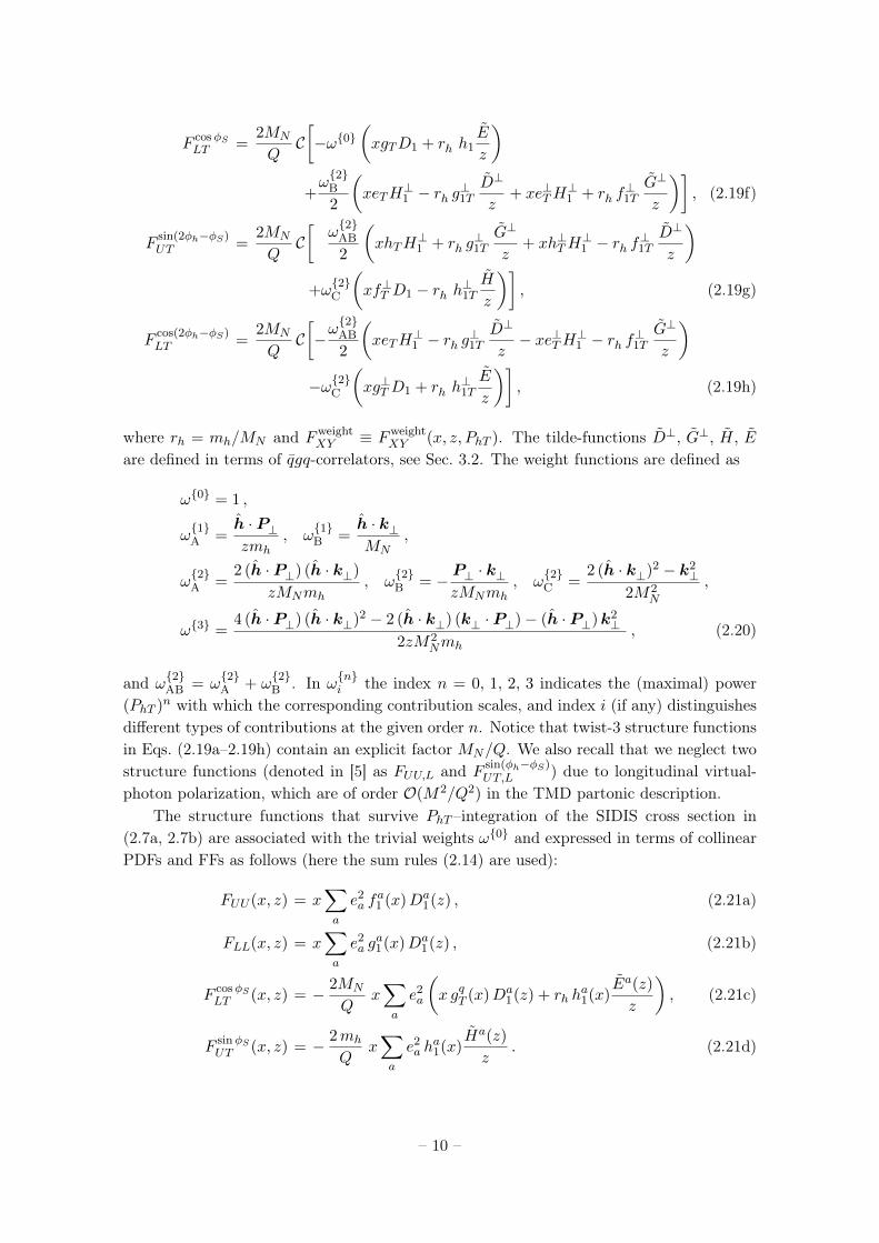
where rh = mh/MN and FweightXY ≡ Fweight
XY (x, z, PhT ). The tilde-functions D⊥, G⊥, H, Eare defined in terms of qgq-correlators, see Sec. 3.2. The weight functions are defined as
ω{0} = 1 ,
ω{1}A =
h · P⊥zmh
, ω{1}B =
h · k⊥MN
,
ω{2}A =
2 (h · P⊥) (h · k⊥)
zMNmh, ω
{2}B = −
P⊥ · k⊥zMNmh
, ω{2}C =
2 (h · k⊥)2 − k2⊥
2M2N
,
ω{3} =4 (h · P⊥) (h · k⊥)2 − 2 (h · k⊥) (k⊥ · P⊥)− (h · P⊥)k2
⊥2zM2
Nmh, (2.20)
and ω{2}AB = ω
{2}A + ω
{2}B . In ω
{n}i the index n = 0, 1, 2, 3 indicates the (maximal) power
(PhT )n with which the corresponding contribution scales, and index i (if any) distinguishesdifferent types of contributions at the given order n. Notice that twist-3 structure functionsin Eqs. (2.19a–2.19h) contain an explicit factor MN/Q. We also recall that we neglect twostructure functions (denoted in [5] as FUU,L and F sin(φh−φS)
UT,L ) due to longitudinal virtual-photon polarization, which are of order O(M2/Q2) in the TMD partonic description.
The structure functions that survive PhT –integration of the SIDIS cross section in(2.7a, 2.7b) are associated with the trivial weights ω{0} and expressed in terms of collinearPDFs and FFs as follows (here the sum rules (2.14) are used):
FUU (x, z) = x∑a
e2a f
a1 (x)Da
1(z) , (2.21a)
FLL(x, z) = x∑a
e2a g
a1(x)Da
1(z) , (2.21b)
F cosφSLT (x, z) = − 2MN
Qx∑a
e2a
(x gqT (x)Da
1(z) + rh ha1(x)
Ea(z)
z
), (2.21c)
F sinφSUT (x, z) = − 2mh
Qx∑a
e2a h
a1(x)
Ha(z)
z. (2.21d)
– 10 –
Finally, integrating over z, summing over hadrons, and using the sum rules for the T-oddFFs,
∑h
∫dz Ea(z) = 0 and
∑h
∫dz Ha(z) = 0, we recover Eqs. (2.10a–2.10d) and obtain
for the DIS structure functions
F1(x) =1
2
∑a
e2a f
a1 (x) , (2.22a)
g1(x) =1
2
∑a
e2a g
a1(x) , (2.22b)
g2(x) =1
2
∑a
e2a g
aT (x) − g1(x) . (2.22c)
Before introducing the WW-type approximations in the next section, we would liketo add a comment on TMD factorization: the partonic description of the leading-twiststructure functions in (2.18) is based on factorization theorems [39–43]. In contrast to this,the partonic description of the subleading-twist structure functions in (2.19) is based onthe assumption that that SIDIS cross section factorizes.
A lot of progress has been achieved in recent years in the theoretical understanding ofleading-twist observables within the TMD framework, including definition, renormalizationand evolution of leading-twist TMDs [44–47], next-to-leading order corrections within theTMD framework [48], and phenomenological fits with evolution [49, 50]. The matching oftwist-2 collinear and TMD quantities was studied to next-to-leading and next-to-next-to-leading order [51, 52]. The WW approximation has been used recently in Ref. [53] to connectthe twist-2 TMDs f⊥1T , g
⊥1T , h
⊥1 , h⊥1L to certain higher-twist collinear matrix elements.
In contrast to this, the theory for subleading-twist TMD observables is only poorlydeveloped. Still to the present day, the state-of-the-art approach to subleading-twist TMDobservables is the one of Refs. [1–5], based on a TMD tree-level formalism, which we adopthere. In fact, the results of Refs. [34, 35] indicate doubts even in the tree-level formalism.Recently, an attempt was made to remedy these doubts [54]. Keeping in mind these “wordsof warning,” still the formulas (2.19) are the best that theory has to offer currently. Wemay consider (2.19) as a model itself for the twist-3 SIDIS observables. We hope that thephenomenological approach based on WW-type approximations pursued in this work mightlead to more insight into these observables, and eventually might trigger more theory effortsin the future.
3 WW and WW-type approximations
In this section we will define the approximations and review what is known about them.The basic idea of the approximations is simple. One uses QCD equations of motion toseparate contributions from qq–terms and qgq–terms and assumes that the latter can beneglected with respect to the leading qq–terms with a useful accuracy (here the 〈. . .〉 denotesymbolically the matrix elements which enter the definitions of TMDs or FFs):∣∣∣∣〈qgq〉〈qq〉
∣∣∣∣� 1 . (3.1)
– 11 –
3.1 WW approximation for PDFs
The WW approximation applies in principle to all twist-3 PDFs, Eqs. (2.13d, 2.13e, 2.13f).It was established first for gaT (x) [16], and later for haL(x) [17]. The situation of ea(x) issomewhat special, see below and the review [55].
The origin of the approximations is as follows. The operators defining gaT (x) and haL(x)
can be decomposed by means of QCD equations of motion in twist-2 parts, and pure twist-3(interaction dependent) qgq–terms and current-quark mass terms. We denote qgq–termsand mass terms collectively and symbolically by functions with a tilde.1 Such decomposi-tions are possible because gaT (x) and haL(x) are “twist-3” not according to the “strict QCDdefinition” (twist = mass dimension of associated local operator minus its spin). Ratherthey are classified according to the “working definition” of twist [56] (a function is “twist t”if, in addition to overall kinematic prefactors, it contributes to cross sections in a partonicdescription suppressed by (M/Q)t−2 where M is a generic hadronic and Q the hard scale).The two definitions coincide for twist-2 quantities, but higher-twist observables in generalcontain “contaminations” by leading twist.
In this way one obtains the decompositions and, if they apply, WW approximations[16, 17] (keep in mind here tilde terms contain pure twist-3 and current-quark mass terms)
gaT (x) =
∫ 1
x
dy
yga1(y)+gaT (x)
WW≈
∫ 1
x
dy
yga1(y) , (3.2a)
haL(x) = 2x
∫ 1
x
dy
y2ha1(y)+haL(x)
WW≈ 2x
∫ 1
x
dy
y2ha1(y) , (3.2b)
x ea(x) = x ea(x)WW≈ 0 , (3.2c)
where we included ea(x) which is a special case in the sense that it receives no twist-2contribution. A prefactor of x is provided in (3.2c) to cancel a δ(x)–type singularity [55].
The relations (3.2a–3.2c) have been derived basically using operator product expansiontechniques [16, 17]. Notice that the operators defining gaT and and haL can also be decom-posed within the TMD framework by means of a combination of relations derived from theQCD equations of motion and further constraint relations, called Lorentz-invariance rela-tions (LIRs), into a twist-2 part, and dynamical twist-3 (interactions dependent) qgq-termsand current-quark mass terms (see recent review [57] and references therein).
We will come back to (3.2a, 3.2b) and review the theoretical predictions and supportingexperiments, but before we will introduce the WW-type approximations for TMDs and FFs.
3.2 WW-type approximations for TMDs and FFs
Analogous to WW approximations for PDFs discussed in Sec. 3.1, also certain TMDs andFFs can be decomposed into twist-2 contributions and tilde terms. The latter may beassumed, in the spirit of (3.1), to be small. Hereby it is important to keep in mind that for
1In the literature it is customary to reserve the term "tilde terms" for matrix elements of qgq operators asdone, e.g., in Ref [5]. For convenience in this work "tilde terms" refers to both qgq terms and current-quarkmass terms as done, e.g., in [30].
– 12 –
each TMD or FF one deals with different types of (“unintegrated”) qgq–correlations, andwe prefer to refer to them as WW-type approximations.
In the T-even case one obtains the following approximations2, where the terms on theleft-hand-side are twist-3, those on the right-hand-side (if any) are twist-2,
xeq(x, k2⊥)
WW–type≈ 0, (3.3a)
xf⊥q(x, k2⊥)
WW–type≈ f q1 (x, k2
⊥), (3.3b)
xg⊥qL (x, k2⊥)
WW–type≈ gq1(x, k2
⊥), (3.3c)
xg⊥qT (x, k2⊥)
WW–type≈ g⊥q1T (x, k2
⊥), (3.3d)
xgqT (x, k2⊥)
WW–type≈ g
⊥(1)q1T (x, k2
⊥), (3.3e)
xhqL(x, k2⊥)
WW–type≈ −2h
⊥(1)q1L (x, k2
⊥), (3.3f)
xhqT (x, k2⊥)
WW–type≈ −hq1(x, k2
⊥)− h⊥(1)1T (x, k2
⊥), (3.3g)
xh⊥qT (x, k2⊥)
WW–type≈ hq1(x, k2
⊥)− h⊥(1)1T (x, k2
⊥). (3.3h)
In the T-odd case one obtains the approximations
xeqL(x, k2⊥)
WW–type≈ 0, (3.4a)
xeqT (x, k2⊥)
WW–type≈ 0, (3.4b)
xe⊥qT (x, k2⊥)
WW–type≈ 0, (3.4c)
xg⊥q(x, k2⊥)
WW–type≈ 0, (3.4d)
xf⊥qL (x, k2⊥)
WW–type≈ 0, (3.4e)
xf⊥qT (x, k2⊥)
WW–type≈ f⊥q1T (x, k2
⊥), (3.4f)
xf qT (x, k2⊥)
WW–type≈ − f⊥(1)q
1T (x, k2⊥), (3.4g)
xhq(x, k2⊥)
WW–type≈ −2h
⊥(1)1 (x, k2
⊥). (3.4h)
The superscript “(1)” denotes the first transverse moment of TMDs defined generically as
f (1)(x, k2⊥) =
k2⊥
2M2f(x, k2
⊥) , f (1)(x) =
∫d2k⊥f
(1)(x, k2⊥) . (3.5)
Two very useful WW-type approximations follow from combining the WW approxima-tions (3.2a, 3.2b) with the WW-type approximations (3.3e, 3.3f). The resulting relations
2Notice that Ref. [5] uses four-vector notation for transverse vectors, while in this paper we always utilizetwo-vectors for transverse vectors, such that e.g. k2
⊥our = −p2TRef. [5] and analog for other scalar productsof transverse vectors. Notice that in our notation transverse vectors are never understood as four-vectorssuch that k2
⊥our ≡ k2⊥our.
– 13 –
are the only WW-type relations applicable to twist-2 TMDs and are given by the followingexpressions [2, 29, 32]:
g⊥(1)a1T (x)
WW–type≈ x
∫ 1
x
dy
yga1(y) , (3.6a)
h⊥(1)a1L (x)
WW–type≈ −x2
∫ 1
x
dy
y2ha1(y) . (3.6b)
Some of the above WW-type approximations were discussed in [2, 26–32]. WW-relationsfor FFs are actually not needed: in Eqs. (2.18, 2.19) either twist-2 FFs Dq
1, H⊥q1 enter or
tilde FFs, as a consequence of how the azimuthal angles are defined [5]. For completenesswe quote the WW-type approximations for FFs [5]
E(z, P 2⊥)
WW–type≈ 0, (3.7a)
G⊥(z, P 2⊥)
WW–type≈ 0, (3.7b)
D⊥(z, P 2⊥)
WW–type≈ z D1(z, P 2
⊥) , (3.7c)
H(z, P 2⊥)
WW–type≈ −
P 2⊥
zM2h
H⊥1 (z, P 2⊥) . (3.7d)
Having introduced the WW and WW-type approximations, we will review in the followingwhat is currently known from theory and experiment about the WW(-type) approximations.
3.3 Predictions from instanton vacuum model
Insights into the relative size of hadronic matrix elements, such as Eq. (3.1), require anon-perturbative approach. It is by no means obvious which small parameter in the strong-interaction regime would allow one to explain such results. An appealing non-perturbativeapproach is provided by the instanton model of the QCD vacuum [58–60]. This semi-classical approach assumes that properties of the QCD vacuum are dominated by instantonsand anti-instantons, topological non-perturbative gluon field configurations, which form astrongly interacting medium. The approach provides a natural mechanism for dynamicalchiral-symmetry breaking, the dominant feature of strong interactions in the nonperturba-tive regime. It was shown with variational and numerical methods that the instantons forma dilute medium characterized by a non-trivial small parameter ρ/R ∼ 1/3 [58–60], whereρ and R denote respectively the average instanton size ρ and separation R.
Applying the instanton vacuum model to studies of gaT (x) and haL(x), it was predictedthat matrix elements of the qgq operators defining gaT (x) [19] and haL(x) [20] are stronglysuppressed by powers of the small parameter ρ/R with respect to contributions from therespective twist-2 parts, which are of order (ρ/R)0. For Mellin moments it was foundthat [19, 20]
gqTgqT∼hqLhqL∼ 〈qgq〉〈qq〉
∼(ρ
R
)4
log
(ρ
R
)∼ 10−2 , (3.8)
which strongly supports the generic approximation in Eq. (3.1) with the instanton packingfraction providing the non-trivial small parameter justifying the neglect of tilde terms. Thepredictions for gaT (x) [19] were made before the advent of the first precise data on g2(x),which we discuss next. The instanton calculus has not yet been applied to ea(x).
– 14 –
P
N
0.0 0.2 0.4 0.6 0.8 1.0
-0.08
-0.06
-0.04
-0.02
0.00
0.02
0.04
x
xg2(x)
P
0.0 0.2 0.4 0.6 0.8 1.0
-0.2
-0.1
0.0
0.1
0.2
x
xg2(x)
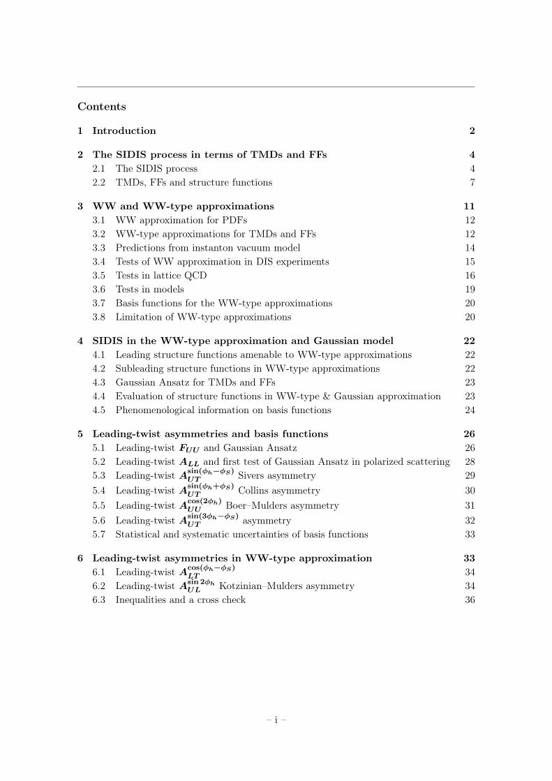
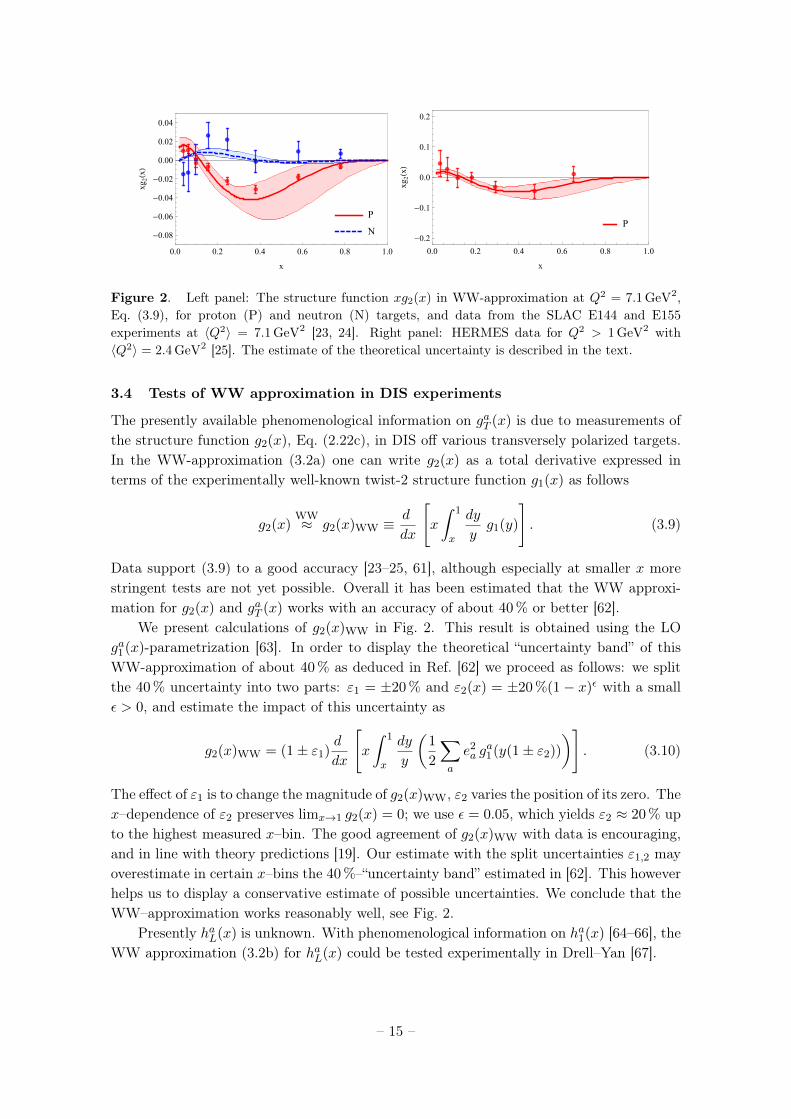
Figure 2. Left panel: The structure function xg2(x) in WW-approximation at Q2 = 7.1 GeV2,Eq. (3.9), for proton (P) and neutron (N) targets, and data from the SLAC E144 and E155experiments at 〈Q2〉 = 7.1 GeV2 [23, 24]. Right panel: HERMES data for Q2 > 1 GeV2 with〈Q2〉 = 2.4 GeV2 [25]. The estimate of the theoretical uncertainty is described in the text.
3.4 Tests of WW approximation in DIS experiments
The presently available phenomenological information on gaT (x) is due to measurements ofthe structure function g2(x), Eq. (2.22c), in DIS off various transversely polarized targets.In the WW-approximation (3.2a) one can write g2(x) as a total derivative expressed interms of the experimentally well-known twist-2 structure function g1(x) as follows
g2(x)WW≈ g2(x)WW ≡
d
dx
[x
∫ 1
x
dy
yg1(y)
]. (3.9)
Data support (3.9) to a good accuracy [23–25, 61], although especially at smaller x morestringent tests are not yet possible. Overall it has been estimated that the WW approxi-mation for g2(x) and gaT (x) works with an accuracy of about 40 % or better [62].
We present calculations of g2(x)WW in Fig. 2. This result is obtained using the LOga1(x)-parametrization [63]. In order to display the theoretical “uncertainty band” of thisWW-approximation of about 40 % as deduced in Ref. [62] we proceed as follows: we splitthe 40 % uncertainty into two parts: ε1 = ±20 % and ε2(x) = ±20 %(1 − x)ε with a smallε > 0, and estimate the impact of this uncertainty as
g2(x)WW = (1± ε1)d
dx
[x
∫ 1
x
dy
y
(1
2
∑a
e2a g
a1(y(1± ε2))
)]. (3.10)
The effect of ε1 is to change the magnitude of g2(x)WW, ε2 varies the position of its zero. Thex–dependence of ε2 preserves limx→1 g2(x) = 0; we use ε = 0.05, which yields ε2 ≈ 20 % upto the highest measured x–bin. The good agreement of g2(x)WW with data is encouraging,and in line with theory predictions [19]. Our estimate with the split uncertainties ε1,2 mayoverestimate in certain x–bins the 40 %–“uncertainty band” estimated in [62]. This howeverhelps us to display a conservative estimate of possible uncertainties. We conclude that theWW–approximation works reasonably well, see Fig. 2.
Presently haL(x) is unknown. With phenomenological information on ha1(x) [64–66], theWW approximation (3.2b) for haL(x) could be tested experimentally in Drell–Yan [67].
– 15 –
3.5 Tests in lattice QCD
The lowest Mellin moments of the PDF gqT (x) were studied in lattice QCD in the quenchedapproximation [21] and with Nf = 2 flavors of light dynamical quarks [22]. The resultsobtained were compatible with a small gqT (x). We are not aware of lattice QCD studiesrelated to the PDF haL(x), and turn now our attention to TMD studies in lattice QCD.
After first exploratory investigations of TMDs on the lattice [68, 69], recent yearshave witnessed considerable progress and improvements with regard to rigor, realism andmethodology [70–73]. However, numerical results from recent calculations are only availablefor a subset of observables, and the quantities calculated are not in a form that lendsitself to straightforward tests of the WW-type relations as presented in this paper. Thisassumption holds if renormalization is multiplicative and flavor-independent for the non-local lattice operators. This is not true for all lattice actions [69]. But presumably it is trueif the lattice action preserves chiral symmetry, as it does in the present case. For the latestdevelopments we refer the interested reader to Refs. [70–78].
For the time being, we content ourselves with rather crude comparisons based on thelattice data published in Refs. [68, 69]. These early works explored all nucleon and quarkpolarizations, but they used a gauge link that does not incorporate the final or initial stateinteractions present in SIDIS or Drell–Yan experiments. In other words, the transverse mo-mentum dependent quantities computed in [68, 69] are not precisely the TMDs measurablein experiment. More caveats will be discussed along the way.
Let us now translate the approximations (3.6a, 3.6b) into expressions for which wehave a chance to compare them with available lattice data. For that we multiply theEqs. (3.6a, 3.6b) by xN with N = 0, 1, 2, . . . and integrate over x ∈ [−1, 1] which yields∫ 1
−1dx xNg
⊥(1)q1T (x)
WW–type≈ 1
N + 2
∫ 1
−1dx xN+1gq1(x) , (3.11)∫ 1
−1dx xNh
⊥(1)q1L (x)
WW–type≈ − 1
N + 3
∫ 1
−1dx xN+1 hq1(x) . (3.12)
Here the negative x refer to antiquark distributions gq1(x) = + gq1(−x), hq1(x) = −hq1(−x),g⊥(1)q1T (x) = −g⊥(1)q
1T (−x), h⊥(1)q1L (x) = +h
⊥(1)q1L (−x) depending on C–parity of the involved
operators [2]. The right-hand sides of Eqs. (3.11, 3.12) are x–moments of parton distribu-tions, and those can be obtained from lattice QCD using well-established methods basedon operator product expansion. The left-hand sides are moments of TMDs in x and k⊥.We have to keep in mind that TMDs diverge for large k⊥. Therefore, without regularizingthese divergences in a scheme suitable for the comparison of left and right hand side, a testof the above relations is meaningless, even before we get to address the issues of latticecalculations. Let us not give up at this point and take a look at the lattice observables ofRef. [69] where TMDs were obtained from amplitudes Ai(l2, . . .) in Fourier space, wherek⊥ is encoded in the Fourier conjugate variable `⊥, which is the transverse displacementof quark operators in the correlator evaluated on the lattice. In Fourier space, the afore-mentioned divergent behavior for large k⊥ translates into strong lattice scale and schemedependences at short distances `⊥ between the quark operators. The k⊥ integrals needed
– 16 –
for the left-hand sides of Eqs. (3.11, 3.12) correspond to the amplitudes at `⊥ = 0, wherescheme and scale dependence is greatest. In Ref. [69] Gaussian fits have been performed tothe amplitudes excluding data at short quark separations `⊥. The Gaussians describe thelong-range data quite well and bridge the gap at short distances `⊥. Taking the Gaussianfit at `⊥ = 0, we get a value that is (presumably) largely lattice-scheme and scale inde-pendent. We have thus swept the problem of divergences under the rug. The Gaussianfit acts as a crude regularization of the divergences that appear in TMDs at large k⊥ andmanifest themselves as short range artifacts on the lattice. Casting this line of thought intomathematics, we get∫ 1
−1dx g
⊥(1)q1T (x) =
∫ 1
−1dx
∫d2k⊥
k2⊥
2M2g⊥q1T (x, k⊥) = −2A7,q(` = 0)
Gauss= −c7,q (3.13)∫ 1
−1dx h
⊥(1)q1L (x) =
∫ 1
−1dx
∫d2k⊥
k2⊥
2M2h⊥q1T (x, k⊥) = −2A10,q(` = 0)
Gauss= −c10,q (3.14)
where the amplitudes A and constants c are those of Ref. [69]. We have thus expressedthe left-hand side of Eqs. (3.11, 3.12) in terms of amplitudes c7,q and c10,q of the Gaussianfits on the lattice. Before quoting numbers, a few more comments are in order. Theoverall multiplicative renormalization in Ref. [69] was fixed by setting the Gaussian integralc2,u−d of the unpolarized TMD f1 in the isovector channel (u-d) to the nucleon quarkcontent, namely to 1. One then assumes that the normalization of the lattice results for theunpolarized TMD f1 also fixes the normalization for polarized quantities correctly. Thisassumption holds if renormalization is multiplicative and flavor independent for the non-local lattice operators. This is not true for all lattice actions [70] but presumably it is true ifthe lattice action preserves chiral symmetry, as it does in the present case. The Gaussian fitsalong with the normalization prescription serve as a crude form of renormalization, and thisis needed to attempt a comparison of left and right hand sides of equations Eqs. (3.11, 3.12).
There is another issue to discuss. The gauge link that goes into the evaluation of thequark-quark correlator introduces a power divergence that has to be subtracted. Ref. [69]employs a subtraction scheme on the lattice but establishes no connection with a subtractionscheme designed for experimental TMDs and the corresponding gauge-link geometry. Thegauge-link renormalization mainly influences the width of the Gaussian fits; the amplitudesare only slightly affected, so it may not play a big role for our discussion. Altogether, thesignificance of our numerical “tests” of WW relations should be taken with a grain of salt.
For the test of (3.11), we use the numbers∫dx g
⊥(1)u1T (x)
Gauss= −c7,u = 0.1041(85) and∫
dx g⊥(1)d1T (x)
Gauss= −c7,d = −0.0232(42) from [69]. Lattice data for
∫dxxNgq1(x) [79, 80]
and∫dxxNhq1(x) [81] are available for N = 0, 1, 2, 3 . These values have been computed
using (quasi-)local operators that have been renormalized to the MS scheme at the scaleµ2 = 4GeV2. According to [80] (data set 4: with amu,d = 0.020 with mπ ≈ 500 MeV) onehas
∫dx x gu−d1 (x) = 0.257(10) and
∫dx x gu+d
1 (x) = 0.159(14). Decomposing the resultsfrom [80] into individual flavors and inserting them into (3.11), we obtain∫
dx g⊥(1)u1T (x)︸ ︷︷ ︸
=0.1041(85) Ref. [69]
!≈ 1
2
∫dx x gu1 (x)︸ ︷︷ ︸
=0.104(9) Ref. [80]
,
– 17 –
∫dx g
⊥(1)d1T (x)︸ ︷︷ ︸
=−0.0232(42) Ref. [69]
!≈ 1
2
∫dx x gd1(x)︸ ︷︷ ︸
=−0.025(9) Ref. [80]
, (3.15)
which confirms the approximation (3.11) for N = 0 within the statistical uncertaintiesof the lattice calculations. In order to test (3.12) we use
∫dx h
⊥(1)u1L (x)
Gauss= −c10,u =
−0.0881(72) and∫dx h
⊥(1)d1L (x)
Gauss= −c10,d = 0.0137(34) from [69] and the lattice data∫
dx xhu1(x) = 0.28(1) and∫dx xhd1(x) = −0.054(4) from QCDSF [81].3 Inserting these
numbers into (3.12) for the case N = 0 we obtain∫dx h
⊥(1)u1L (x)︸ ︷︷ ︸
=−0.0881(72) Ref. [69]
!≈ − 1
3
∫dx xhu1(x)︸ ︷︷ ︸
=−0.093(3) Ref. [80]
,
∫dx h
⊥(1)d1L (x)︸ ︷︷ ︸
=0.0137(34) Ref. [69]
!≈ − 1
3
∫dx xhd1(x)︸ ︷︷ ︸
=0.018(1) Ref. [80]
, (3.16)
which again confirms the WW-type approximation within the statistical uncertainties ofthe lattice calculations.
Several more comments are in order concerning the, at first glance, remarkably goodconfirmation of the WW-type approximations by lattice data in Eqs. (3.15, 3.16).
First, the relations refer to lattice parameters corresponding to pion masses of 500 MeV.We do not need to worry about that too much. The lattice results do provide a valid test ofthe approximations in a “hadronic world” with somewhat heavier pions and nucleons. Allthat matters in our context is that the relative size of qgq–matrix elements is small withrespect to qq–matrix elements.
Second, we have to revisit carefully which approximations the above lattice calculationsactually test. As mentioned above, in the lattice study [68, 69], a specific choice for thepath of the gauge link was chosen, which is actually different from the paths requiredin SIDIS or Drell–Yan. With the path choice of [68, 69] there are effectively only (T-even) Ai amplitudes, the Bi amplitudes are absent. Therefore the test (3.15) of the WW-type approximation (3.11) actually constitutes a test of the WW-approximation (3.2a)and confirms earlier lattice work [21, 22], (cf. Refs. [30, 31] and Sec. 3.6). Similarly, thetest (3.16) of the WW-type approximation (3.12) actually constitutes a test of the WW-approximation (3.2b). The latter, however, has not been reported previously in literature,and constitutes a new result.
Third, to be precise, (3.15, 3.16) test the first Mellin moments of the WW approxi-mations (3.2a, 3.2b), which corresponds to the Burkhardt-Cottingham sum rule for gaT (x)
and an analogous sum rule for haL(x) (see [56] and references therein). In view of the longdebate on the validity of those sum rules [55, 82, 83], this is an interesting result in itself.
3 These numbers are read off from a figure in [81], and were computed on a different lattice. Weinterpolate them to a common value of the pion mass mπ ≈ 500 MeV, and estimate the uncertaintyconservatively in order to take systematic effects into account due to the use of a different lattice.
– 18 –
It is important to stress that in view of the pioneering and exploratory status of theTMD lattice calculations [68, 69], this is already a remarkable and very interesting result.Thus, apart from the instanton calculation [20], also lattice data provide support for thevalidity of the WW approximation (3.2b). At the same time, however, we also have toadmit that we do not really reach our goal of testing the WW-type approximations on thelattice. We have to wait for better lattice data. Meanwhile we may try to gain insights intothe quality of WW-type approximations from models.
3.6 Tests in models
Effective approaches and models such as bag [17, 84–86], spectator [87], chiral quark-soliton[88], or light-cone constituent [89, 90] models support the approximations (3.2a, 3.2b) forPDFs within an accuracy of (10− 30) % at low hadronic scale below 1 GeV.
Turning to TMDs, we recall that in models without gluon degrees of freedom certainrelations among TMDs hold, the so-called quark-model Lorentz-invariance relations (qLIRs)[2, 32].4 Initially thought to be exact [2, 32], qLIRs were shown to be invalid in modelswith gluons [91, 92] and in QCD [93]. They originate from decomposing the (completelyunintegrated) quark correlator in terms of Lorentz-invariant amplitudes, and TMDs arecertain integrals over those amplitudes. When gluons are absent, the correlator consists oftwelve amplitudes [2, 32], i.e., fewer amplitudes than TMDs, which implies relations: theqLIRs. In QCD, the correct Lorentz decomposition requires the consideration of gauge links,which introduces further amplitudes. As a result one has as many amplitudes as TMDsand no relations exist [93]. However, qLIRs “hold” in QCD in the WW-type approximation[30]. In models without gluon degrees of freedom they are exact [30, 31, 86, 87].
The bag, spectator, and light-cone constituent-quark models support the approxima-tions (3.6a, 3.6b) within an accuracy of (10 − 30) % [86, 87, 89, 90]. The spectator andbag model support WW-type approximations within (10− 30) % [86]. As they are definedin terms of quark bilinear expressions (2.11), it is possible to evaluate twist-3 functionsin quark models [17]. The tilde-terms arise due to the different model interactions, andit is important to discuss critically how realistically they describe the qgq–terms of QCD[94, 95].
In the covariant parton model with intrinsic 3D-symmetric parton orbital motion [96],quarks are free, qgq correlations absent, and all WW and WW-type relations exact [97, 98].The phenomenological success of this approach [96] may hint at a general smallness of qgqterms, although some of the predictions from this model have yet to be tested [97].
Noteworthy is the result from the chiral quark-soliton model where the WW-type ap-proximation (3.3b) happens to be exact: xf⊥q(x, k2
⊥) = f q1 (x, k2⊥) for quarks and antiquarks
[94]. The degrees of freedom in this model are quarks, antiquarks, and Goldstone bosons,which are strongly coupled (the coupling constant is ∼ 4) and has to be solved using nonper-turbative techniques (expansion in 1/Nc, where Nc is the number of colors) with the nucleon
4Notice that the qLIRs of [2, 32] are valid only in quark models with no gluons and should not beconfused with the LIRs of [57], which are exact relations in QCD, see Sec. 3.1. In the literature, both areoften simply referred to as LIRs. This ambiguity is unfortunate.
– 19 –
described as a chiral soliton. In general, the model predicts non-zero tilde-terms, for in-stance ea(x) 6= 0 [99–101]. However, despite strong interactions in this effective theory, thetilde term f⊥q(x, k2
⊥) vanishes exactly in this model [94] and the WW-type approximation(3.3b) becomes exact at the low initial scale of this model of µ0 ∼ 0.6 GeV.
Let us finally discuss quark-target models, where gluon degrees of freedom are includedand WW(-type) approximations badly violated [91, 92, 102, 103]. This is natural in thisclass of models for two reasons. First, quark-mass terms are of O(mq/MN ) and negligiblein the nucleon case, but of O(100 %) in a quark target where mq plays also the role ofMN . Second, even if one refrains from mass terms the approximations are spoiled by gluonradiation, see for instance [104] in the context of (3.2a). This means that perturbative QCDdoes not support the WW-approximations: they certainly are not preserved by evolution.However, scaling violations per se do not need to be large. What is crucial in this context aredynamical reasons for the smallness of the matrix elements of qgq–operators. This requiresthe consideration of chiral symmetry breaking effects reflected in the hadronic spectrum, asconsidered in the instanton vacuum model [19, 20] but out of scope in quark-target models.
We are not aware of systematic tests of WW-type approximations for FFs. One infor-mation worth mentioning in this context is that in spectator models [87] tilde-contributionsto FFs are proportional to the offshellness of partons [94, 95]. This natural feature mayindicate that in the region dominated by effects of small P⊥ tilde-terms might be small.On the other hand, quarks have sizable constituent masses of the order of few hundredMeV in spectator models and the mass-terms are not small. The applicability of WW-typeapproximations to FFs remains the least tested point in our approach.
3.7 Basis functions for the WW-type approximations
The 6 leading–twist TMDs fa1 , f⊥a1T , ga1 , h
a1, h
⊥a1 , h⊥a1T and 2 leading–twist FFs Da
1 , H⊥a1
provide a basis in the sense that in WW-type approximation all other TMDs and FFs caneither be expressed in terms of these basis functions or vanish. Below we shall see that,under the assumption of the validity of WW-type approximations, it is possible to expressall SIDIS structure functions in terms of the basis functions.5 These basis functions allowus to describe, in WW-type approximation, all other TMDs. The experiment will tell ushow well the approximations work. In some cases, however, we know in advance that theWW-type approximations have limitations, see next Section 3.8.
3.8 Limitation of WW-type approximations
The approximation may work in the case when the TMD or FF = 〈qq〉+ 〈qgq〉 ≈ 〈qq〉 6= 0
with a “controlled approximation” in the spirit of Eq. (3.1). We know cases where thisworks, see Secs. 3.3, 3.4, but it has to be checked case by case whether |〈qgq〉|� |〈qq〉| fora given operator. At least in such cases the approximation has a chance to work.
5Notice that SIDIS alone is not sufficient to uniquely determine the eight basis functions that appearin six SIDIS leading-twist structure functions. It is thus crucial to take advantage of other processes (likeDrell-Yan and hadron production in e+e− annihilation, which are indispensable for the determination offa1 , Da
1 , H⊥a1 ).
– 20 –
However, it may happen that after applying the QCD equations of motion one endsup in the situation that a given function = 〈qq〉 + 〈qgq〉 with 〈qq〉 = 0. This happens forthe T-even TMD ea in Eqs. (3.2c, 3.3a), for the T-odd TMDs eqL, e
qT , e
⊥qT , f⊥qL , g⊥q in
Eqs. (3.4a–3.4e), and for the FFs Eq, G⊥q in Eqs. (3.7a, 3.7b) (actually, all twist-3 FFs areaffected, we will discuss this in detail below). In this situation the “leading term” is absent,so neglecting the “subleading (pure twist-3) term” actually constitutes an error of 100 %
even if the neglected matrix element 〈qgq〉 is very small. Notice that this type occurs for allsubleading-twist FFs that enter SIDIS structure functions only in the shape of tilde-FFs, seeSec. 2 and Eqs. (2.19). We shall see that some structure functions are potentially more andothers potentially less affected by this generic limitation. In any case, phenomenologicalwork has to be carried out to find out whether or not the approximation works.
For both FFs and TMDs there are also limitations which go beyond this generic issue.To illustrate this for FFs we recall that both H
⊥(1)q1 and Hq
1 are related to integrals ofan underlying function Hq,=
FU (z, z1) as pointed out in Ref. [57]. Therefore, if one literallyassumed Hq(z) to be zero, this would imply that also H⊥(1)q
1 would vanish, indicating thatthe WW-type approximation has to be used with care for chiral-odd FFs.
Similar limitations exist also for TMDs. This is manifest in particular for those twist-3T-odd TMDs that appear in the decomposition of the correlator (2.11) with no prefactorof k⊥. There are three cases: faT (x, k⊥), ha(x, k⊥), and eaL(x, k⊥). Such TMDs in principlesurvive integration of the correlator over k⊥ and would have PDF counterparts if therewere not the sum rules in Eq. (2.14). These sum rules arise because hypothetical PDFversions of T-odd TMDs vanish: they have a simple straight gauge link along the lightcone,and such objects vanish due to parity and time-reversal symmetry of strong interactions.This argument does not apply to other T-odd TMDs because they drop out from the k⊥–integrated correlator due to explicit factors of, e.g., kj⊥ in the case of the Sivers function.
Let us first discuss the case of faT (x, k⊥). Taking the WW-type approximation (3.4g)literally means x
∫d2k⊥ f
aT (x, k⊥)
!?= −f⊥(1)a
1T (x) 6= 0, at variance with the sum rule (2.14).We have xfaT (x, k⊥) = xfaT (x, k⊥)−f⊥(1)a
1T (x, k⊥) from QCD equations of motion [5], whichyields (3.4g). The point is that in this case it is essential to keep the tilde-function. Thesituation for the chirally and T-odd twist-3 TMD ha(x, k⊥) is analogous. The third functionin (2.14) causes no issues since eaL(x, k⊥) = eaL(x, k⊥) ≈ 0 in WW-type approximation.
Does it mean WW-type approximations fail for faT (x, k⊥) and ha(x, k⊥)? Not neces-sarily! The approximations may work in some but not all regions of k⊥, but the sum rules(2.14) include integration over all k⊥. Notice also that, e.g., f⊥(1),q
1T (x) is related to thesoft-gluon-pole matrix element FFT (x, x) [105, 106], which is a qgq-term that one wouldnaturally neglect in WW-type approximation. In this sense (3.4g) could be consistent.Thus, issues with the sum rules (2.14) do not need to exclude the possibility that the WW-type approximations for faT (x, k⊥) and ha(x, k⊥) in (3.4g, 3.4h) may work at small k⊥ wherewe use them in our TMD approach. This would mean that the UV region is essential torealize the sum rules (2.14). Alternatively, one could also envision the sum rules (2.14) tobe sensitive to the IR region through gluonic or fermionic pole contributions manifest intilde-terms.
– 21 –
Presently too little is known in the theory of subleading-twist TMDs. Below in Sec. 7.6and 7.8 we will present a pragmatic solution for how to deal with the TMDs faT (x, k⊥) andha(x, k⊥) phenomenologically. For now let us keep in mind that one has to keep a vigilanteye on all WW-type approximations, and especially on those for faT (x, k⊥) and ha(x, k⊥).
4 SIDIS in the WW-type approximation and Gaussian model
In this section, we consequently apply the WW and WW-type approximation to SIDIS,and describe our procedure to evaluate the structure functions in this approximation andthe Gaussian Ansatz which we use to model the k⊥ dependence of TMDs.
4.1 Leading structure functions amenable to WW-type approximations
The WW and WW-type approximations are useful for the following two leading-twist struc-ture functions:
Fcos(φh−φS)LT
WW= C
[ω{1}B g⊥1TD1
]∣∣∣∣∣ g⊥a1T → ga1Eq. (3.6a)
, (4.1a)
F sin 2φhUL
WW= C
[ω{2}AB h
⊥1LH
⊥1
]∣∣∣∣∣ h⊥a1L → ha1Eq. (3.6b)
. (4.1b)
4.2 Subleading structure functions in WW-type approximations
In the case of the subleading-twist structure functions the WW-type approximations in(3.3a–3.4h) lead to considerable simplifications. We obtain the approximations
F cosφhUU
WW=
2MN
QC[ω{1}A xhH⊥1 − ω
{1}B x f⊥D1
]∣∣∣∣∣ f⊥a → fa1 , ha → h⊥a1
with Eqs. (3.3b, 3.4h)
(4.2a)
F sinφhUL
WW=
2MN
QC[ω{1}A xhLH
⊥1
]∣∣∣∣∣ haL → h⊥a1L
(3.3f)
(4.2b)
F sinφSUT
WW=
2MN
QC[ω{0} x fTD1 −
ω{2}B
2(xhT − xh⊥T )H⊥1
]∣∣∣∣∣ faT → f⊥a1T ,
haT − h⊥aT → ha1
(3.4g, 3.3g, 3.3h)
(4.2c)
Fsin(2φh−φS)UT
WW=
2MN
QC[ω{2}C x f⊥T D1 +
ω{2}AB
2x(hT + h⊥T )H⊥1
]∣∣∣∣∣ f⊥aT → f⊥a1T ,
(haT + h⊥aT )→ h⊥a1T
(3.4f, 3.3g, 3.3h)
(4.2d)
F sinφhLU
WW= 0 (4.2e)
F cosφSLT
WW=
2MN
QC[−ω{0} x gTD1
]∣∣∣∣∣ gaT → ga1(3.2a)
(4.2f)
– 22 –
F cosφhLL
WW=
2MN
QC[−ω{1}B xg⊥LD1
]∣∣∣∣∣ g⊥aL → ga1(3.3c)
(4.2g)
Fcos(2φh−φS)LT
WW=
2MN
QC[−ω{2}C xg⊥TD1
]∣∣∣∣∣ g⊥aT → ga1(3.3d, 3.6a)
(4.2h)
4.3 Gaussian Ansatz for TMDs and FFs
In this work we will use the so-called Gaussian Ansatz for the TMDs and FFs. This Ansatz,which for a generic TMD or FF is given by
f(x, k2⊥) = f(x)
e−k2⊥/〈k
2⊥〉
π〈k2⊥〉
, D(z, P 2⊥) = D(z)
e−P2⊥/〈P
2⊥〉
π〈P 2⊥〉
, (4.3)
is popular not only because it considerably simplifies the calculations. In fact, all convo-lution integrals of the type (2.17) can be solved analytically with this Ansatz. Far moreimportant is the fact that it works phenomenologically with a good accuracy in many prac-tical applications [107–112]. Of course this Ansatz is only a rough approximation. Forinstance, it is not consistent with general matching expectations for large k⊥ [113].
Nevertheless, if one limits oneself to work in a regime where the transverse momenta (ofhadrons produced in SIDIS, dileptons produced in the Drell–Yan process, etc.) are smallcompared to the hard scale in the process, then the Ansatz works quantitatively very well.The most recent and detailed tests were reported in [110], where the Gaussian Ansatz wasshown to describe the most recent SIDIS data: no deviations were observed within the errorbars of the data provided one takes into account the broadening of the Gaussian widths withincreasing energy [110] according with expectations from QCD [44]. The Gaussian Ansatz isapproximately compatible with the k⊥–shapes obtained from evolution [44] or fits to high-energy Tevatron data on weak-boson production [114]. Effective models at low [86, 89, 90]and high [98] renormalization scales support this Ansatz as a good approximation.
4.4 Evaluation of structure functions in WW-type & Gaussian approximation
The Gaussian Ansatz is compatible with many WW-type approximations, but not all. Thetrivial approximations (3.3a) and (3.4a–3.4e) cause no issue. The Gaussian Ansatz canalso be applied to the nontrivial approximations in Eqs. (3.3b–3.3d) and (3.4f), providedthe corresponding Gaussian widths are defined to be equal to each other: for example, inthe WW-type approximation (3.3b), xf⊥q(x, k2
⊥) ≈ f q1 (x, k2⊥), one may assume Gaussian
k⊥–dependence for f⊥q(x, k2⊥) and for f q1 (x, k2
⊥) as long as the Gaussian widths of thesetwo TMDs are assumed to be equal.
In the case of the approximations (3.3e–3.3h) the situation is different because heretwist-3 TMDs are related to transverse moments of twist-2 TMDs. In such cases the Gaus-sian Ansatz is not compatible with the WW-type approximations: for instance, the approx-imation (3.3e) relates xgqT (x, k2
⊥) ≈ k2⊥2M2
Ngq1T (x, k2
⊥), e.g., if gq1T (x, k2⊥) was exactly Gaussian
then gqT (x, k2⊥) certainly could not be Gaussian. If one wanted to take the Gaussian Ansatz
– 23 –
and WW-type approximations literally, one clearly would deal with an incompatibility.However, we of course must keep in mind that both are approximations.
Some comments are in order to understand how the usage of the Gaussian Ansatz andthe WW-type approximations can be reconciled. First, let us remark that the individualTMDs, say gqT (x, k2
⊥) and gq1T (x, k2⊥) in our example, may each by itself be assumed to be
approximately Gaussian in k⊥, which is supported by quark model calculations [86]. Second,we actually do not need the unintegrated WW-type approximations. For phenomenologicalapplications we can use the WW-type approximations in “integrated form.”
Let us stress that if one took an unintegrated WW-type approximation of the typexgqT (x, k2
⊥) ≈ k2⊥2M2
Ngq1T (x, k2
⊥) literally and assumed both TMDs to be exactly Gaussian,one would find “incompatibilities”, perhaps most strikingly in the limit k⊥ → 0 where theleft-hand side is finite while the right-hand side vanishes. Notice that the failure of theWW-type approximations (3.3e–3.3h) in the limit k⊥ → 0 is not specific to the Gaussianmodel, but a general feature caused by neglecting tilde-terms. This indicates a practicalscheme how to use responsibly the WW-type approximations in Eqs. (3.3e–3.3h).
Our procedure is as follows. In a first step we assume that all TMDs and FFs are(approximately) Gaussian and solve the convolution integrals. In the second step we usethe integrated WW-type approximations to simplify the results for the structure functions.
Notice that in some cases (when T-even TMDs are involved) one could choose a dif-ferent order of the steps: first apply WW-type approximations and then solve convolutionintegrals with Gaussian Ansatz. In general, this would yield different (and bulkier) ana-lytical expressions, but we convinced ourselves that the differences are numerically withinthe accuracy expected for this approach. However, for the structure functions discussedin Secs. 7.6 and 7.8, such an “alternative scheme” would give results at variance with thesum rules for the twist-3 T-odd TMDs in Eq. (2.14), as discussed in Sec. 3.8. The schemepresented here will allow us to implement those sum rules in a convenient and consistentway. We will follow up on this in more detail in Secs. 7.6 and 7.8.
To summarize, our procedure is to solve first the convolution integrals with a GaussianAnsatz, and use then WW-type approximations. When implementing this procedure wewill see that the results for the structure functions can be conveniently expressed in termsof the basis TMDs or their adequate transverse moments.
4.5 Phenomenological information on basis functions
We have seen that the following 6 TMDs and 2 FFs provide a basis (Sec. 3) and allow usto express all SIDIS structure functions (Sec. 4) in WW-type approximation:
basis: fa1 , f⊥a1T , g
a1 , h
a1, h
⊥a1 , h⊥a1T ; Da
1 , H⊥a1 . (4.4)
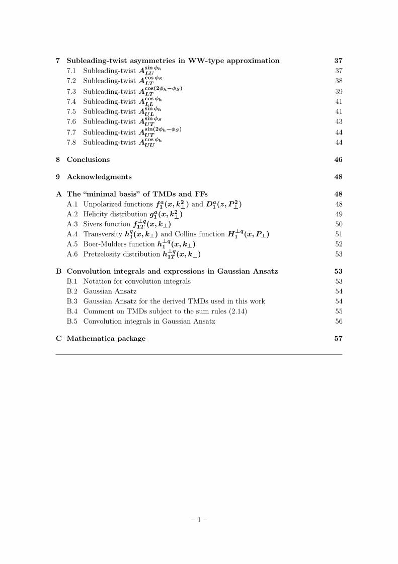
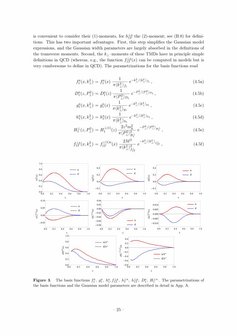
Phenomenological information is available for all basis functions at least to some extent.In Fig. 3 we present plots of the basis functions, and refer to App. A for details. The fourfunctions fa1 , ga1 , ha1, Da
1 are related to twist-2 collinear functions. All collinear functionsare calculated at Q2 = 2.4 GeV2 with fa1 (x) from [115], ga1(x) from [63], and Da
1(z) from[116]. The other four TMDs have no collinear counterparts. For f⊥a1T , h⊥a1 , and H⊥a1 it
– 24 –
is convenient to consider their (1)-moments, for h⊥a1T the (2)-moment; see (B.8) for defini-tions. This has two important advantages. First, this step simplifies the Gaussian modelexpressions, and the Gaussian width parameters are largely absorbed in the definitions ofthe transverse moments. Second, the k⊥–moments of these TMDs have in principle simpledefinitions in QCD (whereas, e.g., the function f⊥a1T (x) can be computed in models but isvery cumbersome to define in QCD). The parametrizations for the basis functions read
fa1 (x, k2⊥) = fa1 (x)
1
π〈k2⊥〉f1
e−k2⊥/〈k
2⊥〉f1 , (4.5a)
Da1(z, P 2
⊥) = Da1(z)
1
π〈P 2⊥〉D1
e−P2⊥/〈P
2⊥〉D1 , (4.5b)
ga1(x, k2⊥) = ga1(x)
1
π〈k2⊥〉g1
e−k2⊥/〈k
2⊥〉g1 , (4.5c)
ha1(x, k2⊥) = ha1(x)
1
π〈k2⊥〉h1
e−k2⊥/〈k
2⊥〉h1 , (4.5d)
H⊥1 (z, P 2⊥) = H
⊥(1)1 (z)
2z2m2h
π〈P 2⊥〉2H⊥1
e−P 2⊥/〈P
2⊥〉H⊥1 , (4.5e)
f⊥a1T (x, k2⊥) = f
⊥(1)a1T (x)
2M2
π〈k2⊥〉2f⊥1T
e−k2⊥/〈k
2⊥〉f⊥
1T , (4.5f)
u
d
0.0 0.2 0.4 0.6 0.8 1.00.0
0.2
0.4
0.6
0.8
1.0
x
xf1q(x)
u
d
0.0 0.2 0.4 0.6 0.8 1.0
-0.2
0.0
0.2
0.4
x
xg1q(x)
u
d
0.0 0.2 0.4 0.6 0.8 1.0
-0.2
0.0
0.2
0.4
x
xh1q(x)
u
d
0.0 0.2 0.4 0.6 0.8 1.0
-0.05
0.00
0.05
0.10
x
xf1T
⊥(1)q (x)
u
d
0.0 0.2 0.4 0.6 0.8 1.0
-0.08
-0.06
-0.04
-0.02
0.00
0.02
0.04
x
xh1⊥(1)q (x)
u
d
0.0 0.2 0.4 0.6 0.8 1.0
-0.010
-0.005
0.000
0.005
0.010
x
xh1T
⊥(2)q (x)
u/π+
d/π+
0.0 0.2 0.4 0.6 0.8 1.00.0
0.2
0.4
0.6
0.8
1.0
z
zD1q/π(z)
u/π+
d/π+
0.0 0.2 0.4 0.6 0.8 1.0-0.8
-0.6
-0.4
-0.2
0.0
0.2
0.4
z
zH1⊥(1)q/π(z)
Figure 3. The basis functions fa1 , ga1 , ha1 , f⊥a1T , h⊥a1 , h⊥a1T ; Da
1 , H⊥a1 . The parametrizations of
the basis functions and the Gaussian model parameters are described in detail in App. A.
– 25 –
h⊥a1 (x, k2⊥) = h
⊥(1)a1 (x)
2M2
π〈k2⊥〉2h⊥1
e−k2⊥/〈k
2⊥〉h⊥1 , (4.5g)
h⊥a1T (x, k2⊥) = h
⊥(2)a1T (x)
2M4
π〈k2⊥〉3h⊥1T
e−k2⊥/〈k
2⊥〉h⊥
1T . (4.5h)
5 Leading-twist asymmetries and basis functions
In this section we review how the basis functions describe available SIDIS data. This is ofimportance to assess the reliability of the predictions presented in the next sections.
5.1 Leading-twist FUU and Gaussian Ansatz
As explained in Sec. 4.3 the Gaussian Ansatz is chosen not only because it considerablysimplifies the calculations, but more importantly because it works phenomenologically witha good accuracy in many processes including SIDIS [107–112].
The Gaussian Ansatz for the unpolarized TMD and FF is given by Eqs. (4.5a, 4.5b).The parameters 〈k2
⊥〉f1 and 〈P 2⊥〉D1 can be assumed to be flavor- and x– or z–independent,
as present data hardly allow us to constrain too many parameters, see App. A.1 for a review.This assumption can be relaxed, e.g., theoretical studies in chiral effective theories predicta strong flavor-dependence in the k⊥–behavior of sea and valence quark TMDs [117].
The structure function FUU needed for our analysis reads
FUU (x, z, PhT ) = x∑q
e2q f
q1 (x)Dq
1(z)G(PhT ) , (5.1a)
FUU (x, z) = x∑q
e2q f
q1 (x)Dq
1(z) , (5.1b)
where we introduce the notation G(PhT ), which is defined as
G(PhT ) =exp(−P 2
hT /λ)
π λ, λ = z2 〈k2
⊥〉f1 + 〈P 2⊥〉D1 , (5.2)
with the understanding that the convenient abbreviation λ is expressed in terms of theGaussian widths of the preceding TMD and FF. Notice that G(PhT ) ≡ G(x, z, PhT ) andthat in general G(PhT ) appears under the flavor sum due to a possible flavor-dependence ofthe involved Gaussian widths. The normalization
∫d2PhT G(PhT ) = 1 correctly connects
the structure function FUU (x, z, PhT ) in (5.1a) with its PhT –integrated counterpart (5.1b).In our effective description this step is trivial. In QCD the connection of TMDs to PDFs issubtle [118]. Figure 4 illustrates how the Gaussian Ansatz describes selected SIDIS data.
Let us begin with JLab where, in the pre-12GeV era, electron beams from CEBAFwith energies in the range 4.3 to 5.7 GeV were scattered off proton or deuterium targetsin the typical kinematics 1 GeV2 < Q2 < 4.5 GeV2, W > 2 GeV, 0.1 < x < 0.6, y < 0.85,0.5 < z < 0.8. The left panel of Fig. 4 shows basically the SIDIS structure functionFUU (P 2
hT ) normalized with respect to its value at zero transverse hadron momentum6 for6Strictly speaking in [119] data for the normalized SIDIS cross section was presented. But these data
correspond to FUU (P 2hT )/FUU (0) ≡ FUU (〈x〉, 〈z〉, P 2
hT )/FUU (〈x〉, 〈z〉, 0) up to 1/Q2-suppressed terms.
– 26 –
π+
0.0 0.2 0.4 0.6 0.8 1.0
10-2
10-1
100
PhT2 (GeV2)
σ(PhT2)/σ(0)
π+
0.0 0.2 0.4 0.6 0.8 1.0 1.2
0
1
2
3
4
PhT(GeV)
Mnh
h+
0.0 0.2 0.4 0.6 0.8 1.0 1.20
2
4
6
8
PhT2 (GeV2)
nh
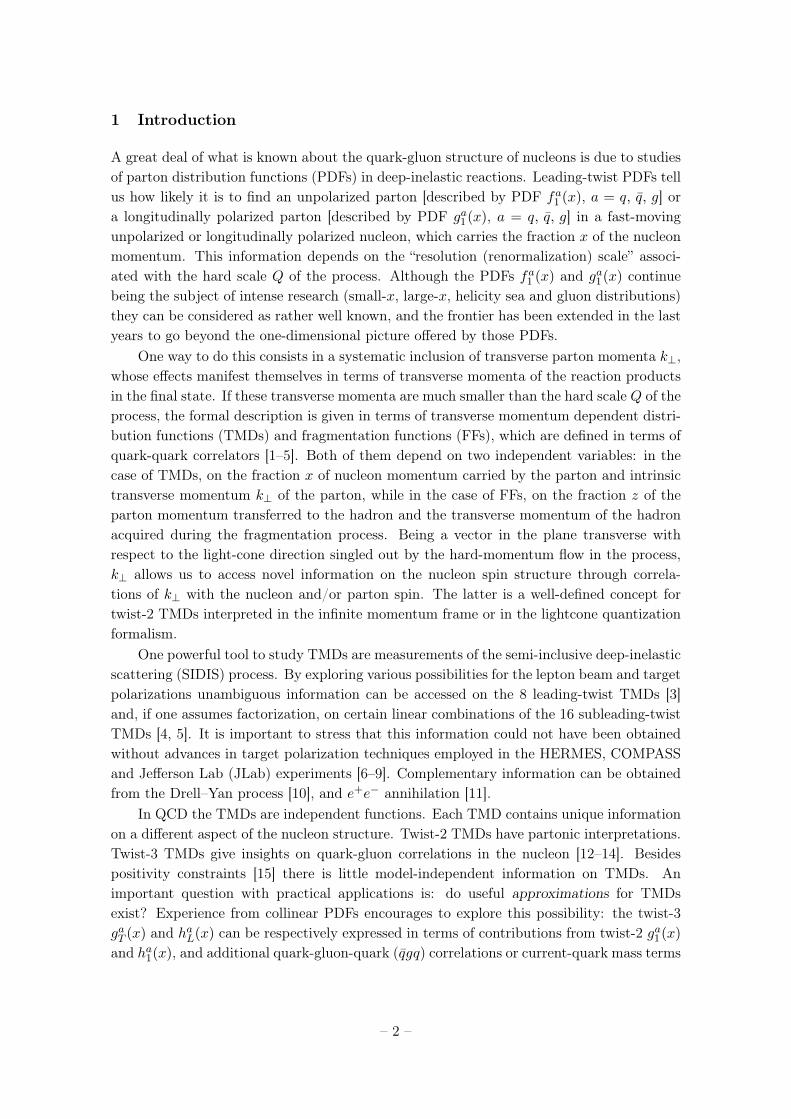
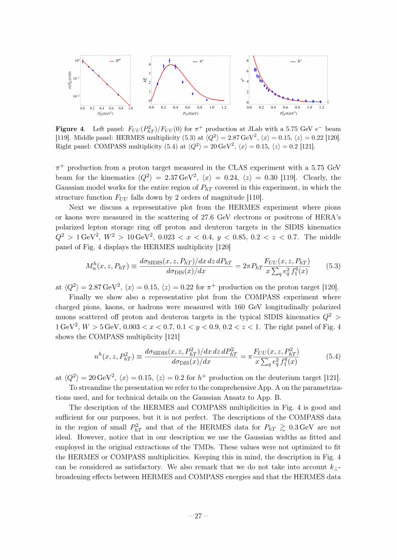
Figure 4. Left panel: FUU (P 2hT )/FUU (0) for π+ production at JLab with a 5.75 GeV e− beam
[119]. Middle panel: HERMES multiplicity (5.3) at 〈Q2〉 = 2.87 GeV2, 〈x〉 = 0.15, 〈z〉 = 0.22 [120].Right panel: COMPASS multiplicity (5.4) at 〈Q2〉 = 20 GeV2, 〈x〉 = 0.15, 〈z〉 = 0.2 [121].
π+ production from a proton target measured in the CLAS experiment with a 5.75 GeVbeam for the kinematics 〈Q2〉 = 2.37 GeV2, 〈x〉 = 0.24, 〈z〉 = 0.30 [119]. Clearly, theGaussian model works for the entire region of PhT covered in this experiment, in which thestructure function FUU falls down by 2 orders of magnitude [110].
Next we discuss a representative plot from the HERMES experiment where pionsor kaons were measured in the scattering of 27.6 GeV electrons or positrons of HERA’spolarized lepton storage ring off proton and deuteron targets in the SIDIS kinematicsQ2 > 1 GeV2, W 2 > 10 GeV2, 0.023 < x < 0.4, y < 0.85, 0.2 < z < 0.7. The middlepanel of Fig. 4 displays the HERMES multiplicity [120]
Mhn (x, z, PhT ) ≡ dσSIDIS(x, z, PhT )/dx dz dPhT
dσDIS(x)/dx= 2πPhT
FUU (x, z, PhT )
x∑
q e2q f
q1 (x)
(5.3)
at 〈Q2〉 = 2.87 GeV2, 〈x〉 = 0.15, 〈z〉 = 0.22 for π+ production on the proton target [120].Finally we show also a representative plot from the COMPASS experiment where
charged pions, kaons, or hadrons were measured with 160 GeV longitudinally polarizedmuons scattered off proton and deuteron targets in the typical SIDIS kinematics Q2 >
1 GeV2, W > 5 GeV, 0.003 < x < 0.7, 0.1 < y < 0.9, 0.2 < z < 1. The right panel of Fig. 4shows the COMPASS multiplicity [121]
nh(x, z, P 2hT ) ≡
dσSIDIS(x, z, P 2hT )/dx dz dP 2
hT
dσDIS(x)/dx= π
FUU (x, z, P 2hT )
x∑
q e2q f
q1 (x)
(5.4)
at 〈Q2〉 = 20 GeV2, 〈x〉 = 0.15, 〈z〉 = 0.2 for h+ production on the deuterium target [121].To streamline the presentation we refer to the comprehensive App. A on the parametriza-
tions used, and for technical details on the Gaussian Ansatz to App. B.The description of the HERMES and COMPASS multiplicities in Fig. 4 is good and
sufficient for our purposes, but it is not perfect. The descriptions of the COMPASS datain the region of small P 2
hT and that of the HERMES data for PhT & 0.3 GeV are notideal. However, notice that in our description we use the Gaussian widths as fitted andemployed in the original extractions of the TMDs. These values were not optimized to fitthe HERMES or COMPASS multiplicities. Keeping this in mind, the description in Fig. 4can be considered as satisfactory. We also remark that we do not take into account k⊥-broadening effects between HERMES and COMPASS energies and that the HERMES data
– 27 –
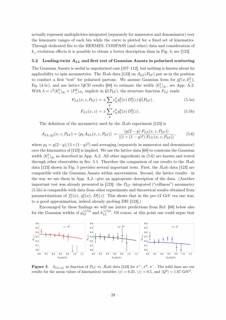
actually represent multiplicities integrated (separately for numerator and denominator) overthe kinematic ranges of each bin while the curve is plotted for a fixed set of kinematics.Through dedicated fits to the HERMES, COMPASS (and other) data and consideration ofk⊥-evolution effects it is possible to obtain a better description than in Fig. 4, see [122].
5.2 Leading-twist ALL and first test of Gaussian Ansatz in polarized scattering
The Gaussian Ansatz is useful in unpolarized case [107–112], but nothing is known about itsapplicability to spin asymmetries. The JLab data [123] on ALL(PhT ) put us in the positionto conduct a first “test” for polarized partons. We assume Gaussian form for ga1(x, k2
⊥),Eq. (4.5c), and use lattice QCD results [68] to estimate the width 〈k2
⊥〉g1 , see App. A.2.With λ = z2〈k2
⊥〉g1 + 〈P 2⊥〉D1 implicit in G(PhT ), the structure function FLL reads
FLL(x, z, PhT ) = x∑q
e2q g
q1(x)Dq
1(z)G(PhT ) , (5.5a)
FLL(x, z) = x∑q
e2q g
q1(x)Dq
1(z) . (5.5b)
The definition of the asymmetry used by the JLab experiment [123] is
ALL,〈y〉(x, z, PhT ) = 〈p2ALL(x, z, PhT )〉 =〈y(2− y) FLL(x, z, PhT )〉
〈(1 + (1− y)2) FUU (x, z, PhT )〉, (5.6)
where p2 = y(2−y)/(1+(1−y)2) and averaging (separately in numerator and denominator)over the kinematics of [123] is implied. We use the lattice data [68] to constrain the Gaussianwidth 〈k2
⊥〉g1 as described in App. A.2. All other ingredients in (5.6) are known and testedthrough other observables in Sec. 5.1. Therefore the comparison of our results to the JLabdata [123] shown in Fig. 5 provides several important tests. First, the JLab data [123] arecompatible with the Gaussian Ansatz within uncertainties. Second, the lattice results—inthe way we use them in App. A.2—give an appropriate description of the data. (Anotherimportant test was already presented in [123]: the PhT –integrated (“collinear”) asymmetry(5.5b) is compatible with data from other experiments and theoretical results obtained fromparametrizations of fa1 (x), ga1(x), Da
1(z). This shows that in the pre-12 GeV era one was,to a good approximation, indeed already probing DIS [123].)
Encouraged by these findings we will use lattice predictions from Ref. [68] below alsofor the Gaussian widths of g⊥(1)a
1T and h⊥(1)a1L . Of course, at this point one could argue that
π+
0.0 0.2 0.4 0.6 0.8 1.0 1.2
0.0
0.1
0.2
0.3
0.4
0.5
0.6
PhT(GeV)
ALL,⟨y⟩
π0
0.0 0.2 0.4 0.6 0.8 1.0 1.2
0.0
0.1
0.2
0.3
0.4
0.5
0.6
PhT(GeV)
ALL,⟨y⟩
π-
0.0 0.2 0.4 0.6 0.8 1.0 1.2
0.0
0.1
0.2
0.3
0.4
0.5
0.6
PhT(GeV)
ALL,⟨y⟩
Figure 5. ALL,〈y〉 as function of PhT vs. JLab data [123] for π+, π0, π−. The solid lines are ourresults for the mean values of kinematical variables 〈x〉 = 0.25, 〈z〉 = 0.5, and 〈Q2〉 = 1.67 GeV2.
– 28 –
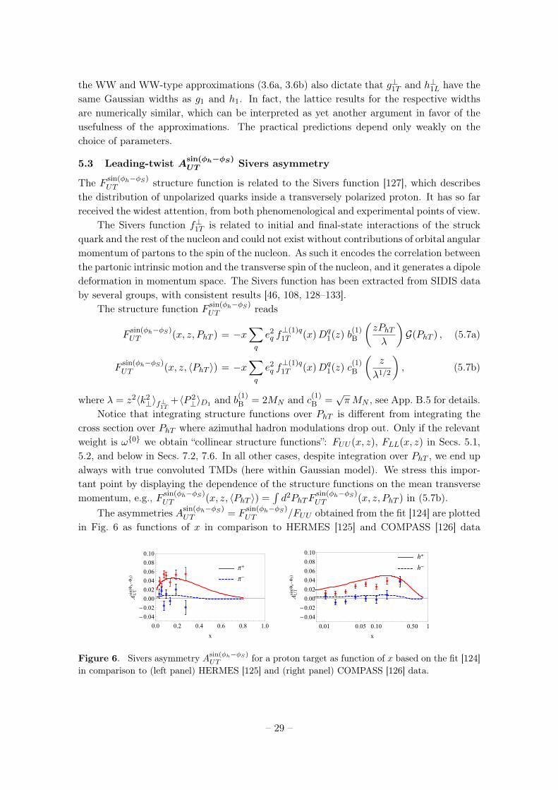
the WW and WW-type approximations (3.6a, 3.6b) also dictate that g⊥1T and h⊥1L have thesame Gaussian widths as g1 and h1. In fact, the lattice results for the respective widthsare numerically similar, which can be interpreted as yet another argument in favor of theusefulness of the approximations. The practical predictions depend only weakly on thechoice of parameters.
5.3 Leading-twist Asin(φh−φS)UT Sivers asymmetry
The F sin(φh−φS)UT structure function is related to the Sivers function [127], which describes
the distribution of unpolarized quarks inside a transversely polarized proton. It has so farreceived the widest attention, from both phenomenological and experimental points of view.
The Sivers function f⊥1T is related to initial and final-state interactions of the struckquark and the rest of the nucleon and could not exist without contributions of orbital angularmomentum of partons to the spin of the nucleon. As such it encodes the correlation betweenthe partonic intrinsic motion and the transverse spin of the nucleon, and it generates a dipoledeformation in momentum space. The Sivers function has been extracted from SIDIS databy several groups, with consistent results [46, 108, 128–133].
The structure function F sin(φh−φS)UT reads
Fsin(φh−φS)UT (x, z, PhT ) = −x
∑q
e2q f⊥(1)q1T (x)Dq
1(z) b(1)B
(zPhTλ
)G(PhT ) , (5.7a)
Fsin(φh−φS)UT (x, z, 〈PhT 〉) = −x
∑q
e2q f⊥(1)q1T (x)Dq
1(z) c(1)B
(z
λ1/2
), (5.7b)
where λ = z2〈k2⊥〉f⊥1T +〈P 2
⊥〉D1 and b(1)B = 2MN and c(1)
B =√πMN , see App. B.5 for details.
Notice that integrating structure functions over PhT is different from integrating thecross section over PhT where azimuthal hadron modulations drop out. Only if the relevantweight is ω{0} we obtain “collinear structure functions”: FUU (x, z), FLL(x, z) in Secs. 5.1,5.2, and below in Secs. 7.2, 7.6. In all other cases, despite integration over PhT , we end upalways with true convoluted TMDs (here within Gaussian model). We stress this impor-tant point by displaying the dependence of the structure functions on the mean transversemomentum, e.g., F sin(φh−φS)
UT (x, z, 〈PhT 〉) =∫d2PhTF
sin(φh−φS)UT (x, z, PhT ) in (5.7b).
The asymmetries Asin(φh−φS)UT = F
sin(φh−φS)UT /FUU obtained from the fit [124] are plotted
in Fig. 6 as functions of x in comparison to HERMES [125] and COMPASS [126] data
π+
π-
0.0 0.2 0.4 0.6 0.8 1.0
-0.04
-0.02
0.00
0.02
0.04
0.06
0.08
0.10
x
AUTsin(Φh-ΦS)
h+
h-
0.01 0.05 0.10 0.50 1
-0.04
-0.02
0.00
0.02
0.04
0.06
0.08
0.10
x
AUTsin(Φh-ΦS)
Figure 6. Sivers asymmetry Asin(φh−φS)UT for a proton target as function of x based on the fit [124]
in comparison to (left panel) HERMES [125] and (right panel) COMPASS [126] data.
– 29 –
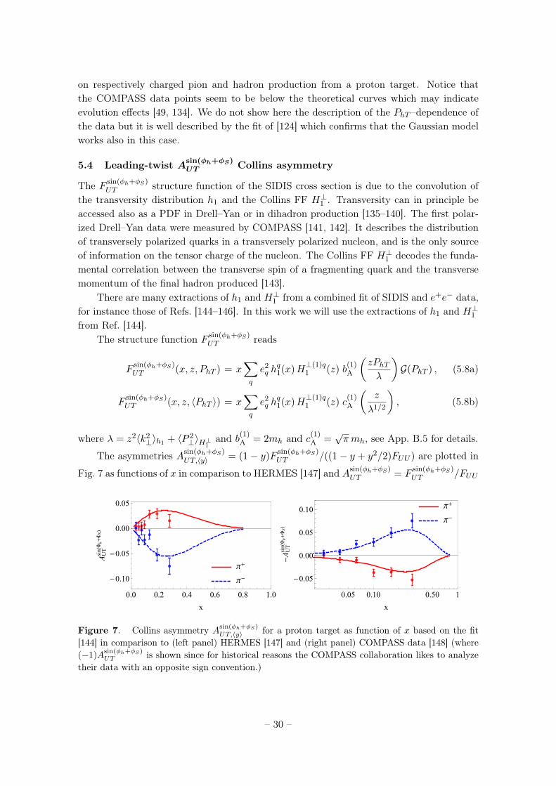
on respectively charged pion and hadron production from a proton target. Notice thatthe COMPASS data points seem to be below the theoretical curves which may indicateevolution effects [49, 134]. We do not show here the description of the PhT –dependence ofthe data but it is well described by the fit of [124] which confirms that the Gaussian modelworks also in this case.
5.4 Leading-twist Asin(φh+φS)UT Collins asymmetry
The F sin(φh+φS)UT structure function of the SIDIS cross section is due to the convolution of
the transversity distribution h1 and the Collins FF H⊥1 . Transversity can in principle beaccessed also as a PDF in Drell–Yan or in dihadron production [135–140]. The first polar-ized Drell–Yan data were measured by COMPASS [141, 142]. It describes the distributionof transversely polarized quarks in a transversely polarized nucleon, and is the only sourceof information on the tensor charge of the nucleon. The Collins FF H⊥1 decodes the funda-mental correlation between the transverse spin of a fragmenting quark and the transversemomentum of the final hadron produced [143].
There are many extractions of h1 and H⊥1 from a combined fit of SIDIS and e+e− data,for instance those of Refs. [144–146]. In this work we will use the extractions of h1 and H⊥1from Ref. [144].
The structure function F sin(φh+φS)UT reads
Fsin(φh+φS)UT (x, z, PhT ) = x
∑q
e2q h
q1(x)H
⊥(1)q1 (z) b
(1)A
(zPhTλ
)G(PhT ) , (5.8a)
Fsin(φh+φS)UT (x, z, 〈PhT 〉) = x
∑q
e2q h
q1(x)H
⊥(1)q1 (z) c
(1)A
(z
λ1/2
), (5.8b)
where λ = z2〈k2⊥〉h1 + 〈P 2
⊥〉H⊥1 and b(1)A = 2mh and c(1)
A =√πmh, see App. B.5 for details.
The asymmetries Asin(φh+φS)UT,〈y〉 = (1− y)F
sin(φh+φS)UT /((1− y + y2/2)FUU ) are plotted in
Fig. 7 as functions of x in comparison to HERMES [147] and Asin(φh+φS)UT = F
sin(φh+φS)UT /FUU
π+
π-
0.0 0.2 0.4 0.6 0.8 1.0
-0.10
-0.05
0.00
0.05
x
AUTsin(Φh+ΦS)
π+
π-
0.05 0.10 0.50 1
-0.05
0.00
0.05
0.10
x
-AUTsin(Φh+ΦS)
Figure 7. Collins asymmetry Asin(φh+φS)UT,〈y〉 for a proton target as function of x based on the fit
[144] in comparison to (left panel) HERMES [147] and (right panel) COMPASS data [148] (where(−1)A
sin(φh+φS)UT is shown since for historical reasons the COMPASS collaboration likes to analyze
their data with an opposite sign convention.)
– 30 –
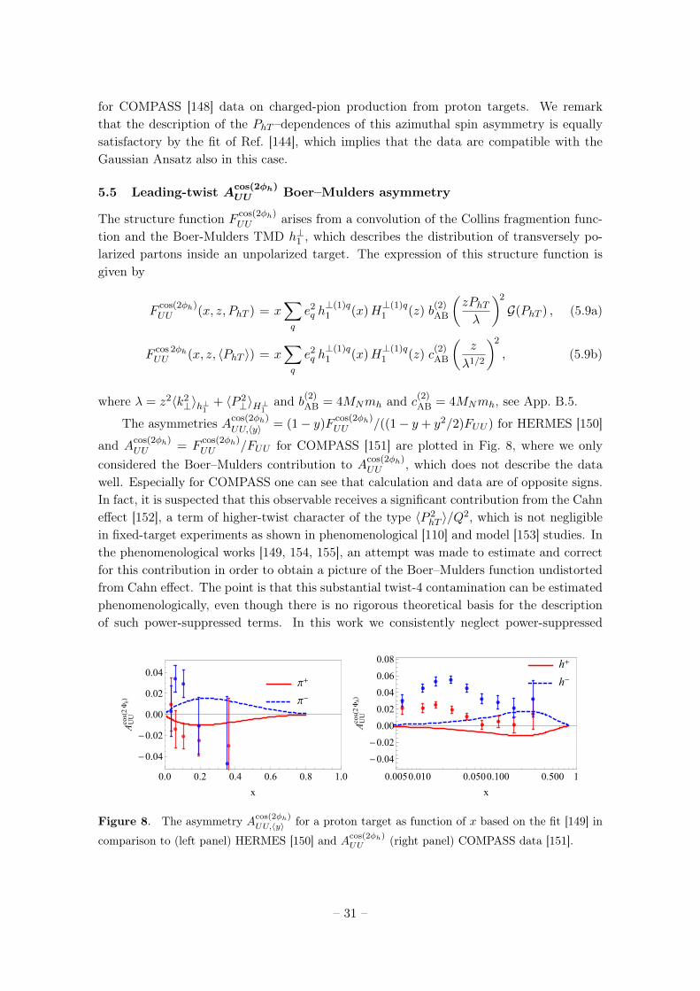
for COMPASS [148] data on charged-pion production from proton targets. We remarkthat the description of the PhT –dependences of this azimuthal spin asymmetry is equallysatisfactory by the fit of Ref. [144], which implies that the data are compatible with theGaussian Ansatz also in this case.
5.5 Leading-twist Acos(2φh)UU Boer–Mulders asymmetry
The structure function F cos(2φh)UU arises from a convolution of the Collins fragmention func-
tion and the Boer-Mulders TMD h⊥1 , which describes the distribution of transversely po-larized partons inside an unpolarized target. The expression of this structure function isgiven by
Fcos(2φh)UU (x, z, PhT ) = x
∑q
e2q h⊥(1)q1 (x)H
⊥(1)q1 (z) b
(2)AB
(zPhTλ
)2
G(PhT ) , (5.9a)
F cos 2φhUU (x, z, 〈PhT 〉) = x
∑q
e2q h⊥(1)q1 (x)H
⊥(1)q1 (z) c
(2)AB
(z
λ1/2
)2
, (5.9b)
where λ = z2〈k2⊥〉h⊥1 + 〈P 2
⊥〉H⊥1 and b(2)AB = 4MNmh and c(2)
AB = 4MNmh, see App. B.5.
The asymmetries Acos(2φh)UU,〈y〉 = (1− y)F
cos(2φh)UU /((1− y + y2/2)FUU ) for HERMES [150]
and Acos(2φh)UU = F
cos(2φh)UU /FUU for COMPASS [151] are plotted in Fig. 8, where we only
considered the Boer–Mulders contribution to Acos(2φh)UU , which does not describe the data
well. Especially for COMPASS one can see that calculation and data are of opposite signs.In fact, it is suspected that this observable receives a significant contribution from the Cahneffect [152], a term of higher-twist character of the type 〈P 2
hT 〉/Q2, which is not negligiblein fixed-target experiments as shown in phenomenological [110] and model [153] studies. Inthe phenomenological works [149, 154, 155], an attempt was made to estimate and correctfor this contribution in order to obtain a picture of the Boer–Mulders function undistortedfrom Cahn effect. The point is that this substantial twist-4 contamination can be estimatedphenomenologically, even though there is no rigorous theoretical basis for the descriptionof such power-suppressed terms. In this work we consistently neglect power-suppressed
π+
π-
0.0 0.2 0.4 0.6 0.8 1.0
-0.04
-0.02
0.00
0.02
0.04
x
AUUcos(2Φh)
h+
h-
0.0050.010 0.0500.100 0.500 1
-0.04
-0.02
0.00
0.02
0.04
0.06
0.08
x
AUUcos(2Φh)
Figure 8. The asymmetry Acos(2φh)UU,〈y〉 for a proton target as function of x based on the fit [149] in
comparison to (left panel) HERMES [150] and Acos(2φh)UU (right panel) COMPASS data [151].
– 31 –
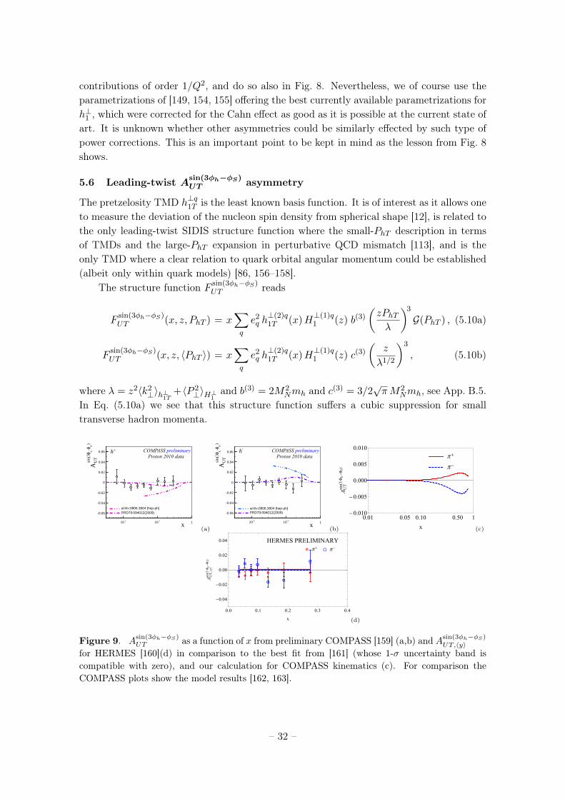
contributions of order 1/Q2, and do so also in Fig. 8. Nevertheless, we of course use theparametrizations of [149, 154, 155] offering the best currently available parametrizations forh⊥1 , which were corrected for the Cahn effect as good as it is possible at the current state ofart. It is unknown whether other asymmetries could be similarly effected by such type ofpower corrections. This is an important point to be kept in mind as the lesson from Fig. 8shows.
5.6 Leading-twist Asin(3φh−φS)UT asymmetry
The pretzelosity TMD h⊥q1T is the least known basis function. It is of interest as it allows oneto measure the deviation of the nucleon spin density from spherical shape [12], is related tothe only leading-twist SIDIS structure function where the small-PhT description in termsof TMDs and the large-PhT expansion in perturbative QCD mismatch [113], and is theonly TMD where a clear relation to quark orbital angular momentum could be established(albeit only within quark models) [86, 156–158].
The structure function F sin(3φh−φS)UT reads
Fsin(3φh−φS)UT (x, z, PhT ) = x
∑q
e2q h⊥(2)q1T (x)H
⊥(1)q1 (z) b(3)
(zPhTλ
)3
G(PhT ) , (5.10a)
Fsin(3φh−φS)UT (x, z, 〈PhT 〉) = x
∑q
e2q h⊥(2)q1T (x)H
⊥(1)q1 (z) c(3)
(z
λ1/2
)3
, (5.10b)
where λ = z2〈k2⊥〉h⊥1T +〈P 2
⊥〉H⊥1 and b(3) = 2M2Nmh and c(3) = 3/2
√πM2
Nmh, see App. B.5.In Eq. (5.10a) we see that this structure function suffers a cubic suppression for smalltransverse hadron momenta.
COMPASS preliminaryProton 2010 data
-210 -110 1
-0.06
-0.04
-0.02
0
0.02
0.04
0.06 h+
)S
-ϕh
sin(
3ϕ
UT
A
x
arXiv:0806.3804 [hep-ph]PRD79:094012(2009)
(a)
COMPASS preliminaryProton 2010 data
-210 -110 1
-0.06
-0.04
-0.02
0
0.02
0.04
0.06-h
)S
-ϕh
sin(
3ϕ
UT
A
x
arXiv:0806.3804 [hep-ph]PRD79:094012(2009)
(b)
π+
π-
0.01 0.05 0.10 0.50 1-0.010
-0.005
0.000
0.005
0.010
x
AUTsin(3Φh-ΦS)
(c)
HERMES PRELIMINARYπ+ π-
0.0 0.1 0.2 0.3 0.4
-0.04
-0.02
0.00
0.02
0.04
x
AUT,⟨y⟩
sin(3Φh-ΦS)
(d)
Figure 9. Asin(3φh−φS)UT as a function of x from preliminary COMPASS [159] (a,b) and Asin(3φh−φS)
UT,〈y〉for HERMES [160](d) in comparison to the best fit from [161] (whose 1-σ uncertainty band iscompatible with zero), and our calculation for COMPASS kinematics (c). For comparison theCOMPASS plots show the model results [162, 163].
– 32 –
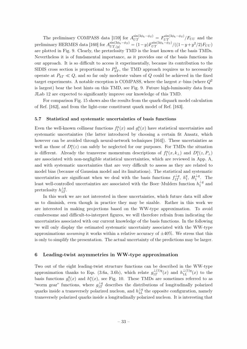
The preliminary COMPASS data [159] for Asin(3φh−φS)UT = F
sin(3φh−φS)UT /FUU and the
preliminary HERMES data [160] for Asin(3φh−φS)UT,〈y〉 = (1−y)F
sin(3φh−φS)UT /((1−y+y2/2)FUU )
are plotted in Fig. 9. Clearly, the pretzelosity TMD is the least known of the basis TMDs.Nevertheless it is of fundamental importance, as it provides one of the basis functions inour approach. It is so difficult to access it experimentally, because its contribution to theSIDIS cross section is proportional to P 3
hT , the TMD approach requires us to necessarilyoperate at PhT � Q, and so far only moderate values of Q could be achieved in the fixedtarget experiments. A notable exception is COMPASS, where the largest x–bins (where Q2
is largest) bear the best hints on this TMD, see Fig. 9. Future high-luminosity data fromJLab 12 are expected to significantly improve our knowledge of this TMD.
For comparison Fig. 15 shows also the results from the quark-diquark model calculationof Ref. [162], and from the light-cone constituent quark model of Ref. [163].
5.7 Statistical and systematic uncertainties of basis functions
Even the well-known collinear functions fa1 (x) and ga1(x) have statistical uncertainties andsystematic uncertainties (the latter introduced by choosing a certain fit Ansatz, whichhowever can be avoided through neural-network techniques [164]). These uncertainties aswell as those of Da
1(z) can safely be neglected for our purposes. For TMDs the situationis different. Already the transverse momentum descriptions of fa1 (x, k⊥) and Da
1(z, P⊥)
are associated with non-negligible statistical uncertainties, which are reviewed in App. A,and with systematic uncertainties that are very difficult to assess as they are related tomodel bias (because of Gaussian model and its limitations). The statistical and systematicuncertainties are significant when we deal with the basis functions f⊥q1T , h
q1, H
⊥q1 . The
least well-controlled uncertainties are associated with the Boer–Mulders function h⊥q1 andpretzelosity h⊥q1T .
In this work we are not interested in these uncertainties, which future data will allowus to diminish, even though in practice they may be sizable. Rather in this work weare interested in making projections based on the WW-type approximation. To avoidcumbersome and difficult-to-interpret figures, we will therefore refrain from indicating theuncertainties associated with our current knowledge of the basis functions. In the followingwe will only display the estimated systematic uncertainty associated with the WW-typeapproximations assuming it works within a relative accuracy of ±40%. We stress that thisis only to simplify the presentation. The actual uncertainty of the predictions may be larger.
6 Leading-twist asymmetries in WW-type approximation
Two out of the eight leading-twist structure functions can be described in the WW-typeapproximation thanks to Eqs. (3.6a, 3.6b), which relate g⊥(1)q
1T (x) and h⊥(1)q1L (x) to the
basis functions gq1(x) and ha1(x), see Fig. 10. These TMDs are sometimes referred to as“worm gear” functions, where g⊥q1T describes the distributions of longitudinally polarizedquarks inside a transversely polarized nucleon, and h⊥q1L the opposite configuration, namelytransversely polarized quarks inside a longitudinally polarized nucleon. It is interesting that
– 33 –
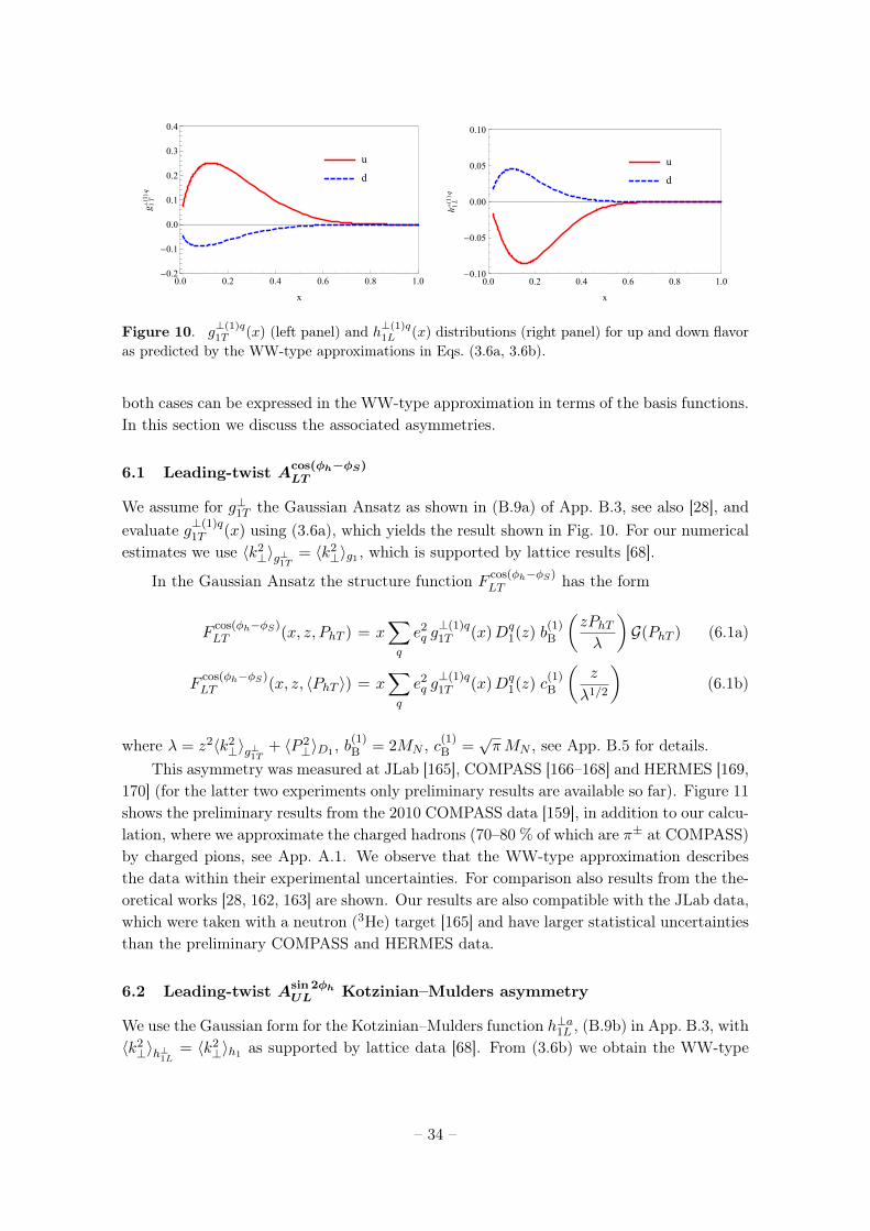
u
d
0.0 0.2 0.4 0.6 0.8 1.0-0.2
-0.1
0.0
0.1
0.2
0.3
0.4
x
g 1T
⊥(1)q
u
d
0.0 0.2 0.4 0.6 0.8 1.0-0.10
-0.05
0.00
0.05
0.10
x
h 1L
⊥(1)q
Figure 10. g⊥(1)q1T (x) (left panel) and h⊥(1)q1L (x) distributions (right panel) for up and down flavor
as predicted by the WW-type approximations in Eqs. (3.6a, 3.6b).
both cases can be expressed in the WW-type approximation in terms of the basis functions.In this section we discuss the associated asymmetries.
6.1 Leading-twist Acos(φh−φS)LT
We assume for g⊥1T the Gaussian Ansatz as shown in (B.9a) of App. B.3, see also [28], andevaluate g⊥(1)q
1T (x) using (3.6a), which yields the result shown in Fig. 10. For our numericalestimates we use 〈k2
⊥〉g⊥1T = 〈k2⊥〉g1 , which is supported by lattice results [68].
In the Gaussian Ansatz the structure function F cos(φh−φS)LT has the form
Fcos(φh−φS)LT (x, z, PhT ) = x
∑q
e2q g⊥(1)q1T (x)Dq
1(z) b(1)B
(zPhTλ
)G(PhT ) (6.1a)
Fcos(φh−φS)LT (x, z, 〈PhT 〉) = x
∑q
e2q g⊥(1)q1T (x)Dq
1(z) c(1)B
(z
λ1/2
)(6.1b)
where λ = z2〈k2⊥〉g⊥1T + 〈P 2
⊥〉D1 , b(1)B = 2MN , c
(1)B =
√πMN , see App. B.5 for details.
This asymmetry was measured at JLab [165], COMPASS [166–168] and HERMES [169,170] (for the latter two experiments only preliminary results are available so far). Figure 11shows the preliminary results from the 2010 COMPASS data [159], in addition to our calcu-lation, where we approximate the charged hadrons (70–80 % of which are π± at COMPASS)by charged pions, see App. A.1. We observe that the WW-type approximation describesthe data within their experimental uncertainties. For comparison also results from the the-oretical works [28, 162, 163] are shown. Our results are also compatible with the JLab data,which were taken with a neutron (3He) target [165] and have larger statistical uncertaintiesthan the preliminary COMPASS and HERMES data.
6.2 Leading-twist Asin 2φhUL Kotzinian–Mulders asymmetry
We use the Gaussian form for the Kotzinian–Mulders function h⊥a1L , (B.9b) in App. B.3, with〈k2⊥〉h⊥1L = 〈k2
⊥〉h1 as supported by lattice data [68]. From (3.6b) we obtain the WW-type
– 34 –
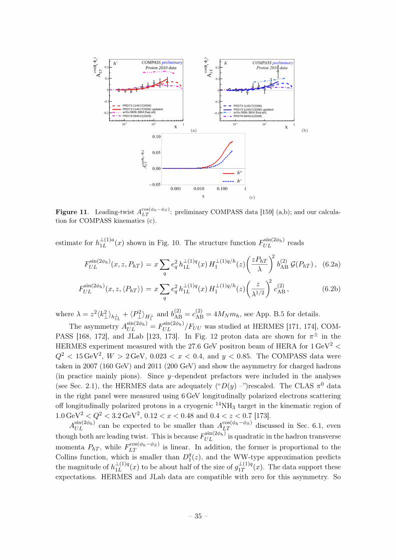
-210 -110 1
-0.2
-0.1
0
0.1
0.2preliminaryCOMPASS +h
Proton 2010 data
)Sϕ-
hϕco
s(
LTA
x
PRD73:114017(2006)
arXiv:0806.3804 [hep-ph]PRD79:094012(2009)
PRD73:114017(2006) updated
(a)
-210 -110 1
-0.2
-0.1
0
0.1
0.2COMPASS preliminary-h
)S
-ϕh
cos(
ϕLT
A
x
PRD73:114017(2006)PRD73:114017(2006) updatedarXiv:0806.3804 [hep-ph]PRD79:094012(2009)
Proton 2010 data
(b)
h+
h-
0.001 0.010 0.100 1-0.05
0.00
0.05
0.10
x
ALTcos(Φh-ΦS)
(c)
Figure 11. Leading-twist Acos(φh−φS)LT : preliminary COMPASS data [159] (a,b); and our calcula-
tion for COMPASS kinematics (c).
estimate for h⊥(1)a1L (x) shown in Fig. 10. The structure function F sin(2φh)
UL reads
Fsin(2φh)UL (x, z, PhT ) = x
∑q
e2q h⊥(1)q1L (x)H
⊥(1)q/h1 (z)
(zPhTλ
)2
b(2)AB G(PhT ) , (6.2a)
Fsin(2φh)UL (x, z, 〈PhT 〉) = x
∑q
e2q h⊥(1)q1L (x)H
⊥(1)q/h1 (z)
(z
λ1/2
)2
c(2)AB , (6.2b)
where λ = z2〈k2⊥〉h⊥1L + 〈P 2
⊥〉H⊥1 and b(2)AB = c
(2)AB = 4MNmh, see App. B.5 for details.
The asymmetry Asin(2φh)UL = F
sin(2φh)UL /FUU was studied at HERMES [171, 174], COM-
PASS [168, 172], and JLab [123, 173]. In Fig. 12 proton data are shown for π± in theHERMES experiment measured with the 27.6 GeV positron beam of HERA for 1 GeV2 <
Q2 < 15 GeV2, W > 2 GeV, 0.023 < x < 0.4, and y < 0.85. The COMPASS data weretaken in 2007 (160 GeV) and 2011 (200 GeV) and show the asymmetry for charged hadrons(in practice mainly pions). Since y–dependent prefactors were included in the analyses(see Sec. 2.1), the HERMES data are adequately (“D(y) –”)rescaled. The CLAS π0 datain the right panel were measured using 6GeV longitudinally polarized electrons scatteringoff longitudinally polarized protons in a cryogenic 14NH3 target in the kinematic region of1.0 GeV2 < Q2 < 3.2 GeV2, 0.12 < x < 0.48 and 0.4 < z < 0.7 [173].
Asin(2φh)UL can be expected to be smaller than A
cos(φh−φS)LT discussed in Sec. 6.1, even
though both are leading twist. This is because F sin(2φh)UL is quadratic in the hadron transverse
momenta PhT , while Fcos(φh−φS)LT is linear. In addition, the former is proportional to the
Collins function, which is smaller than Dq1(z), and the WW-type approximation predicts
the magnitude of h⊥(1)q1L (x) to be about half of the size of g⊥(1)q
1T (x). The data support theseexpectations. HERMES and JLab data are compatible with zero for this asymmetry. So
– 35 –
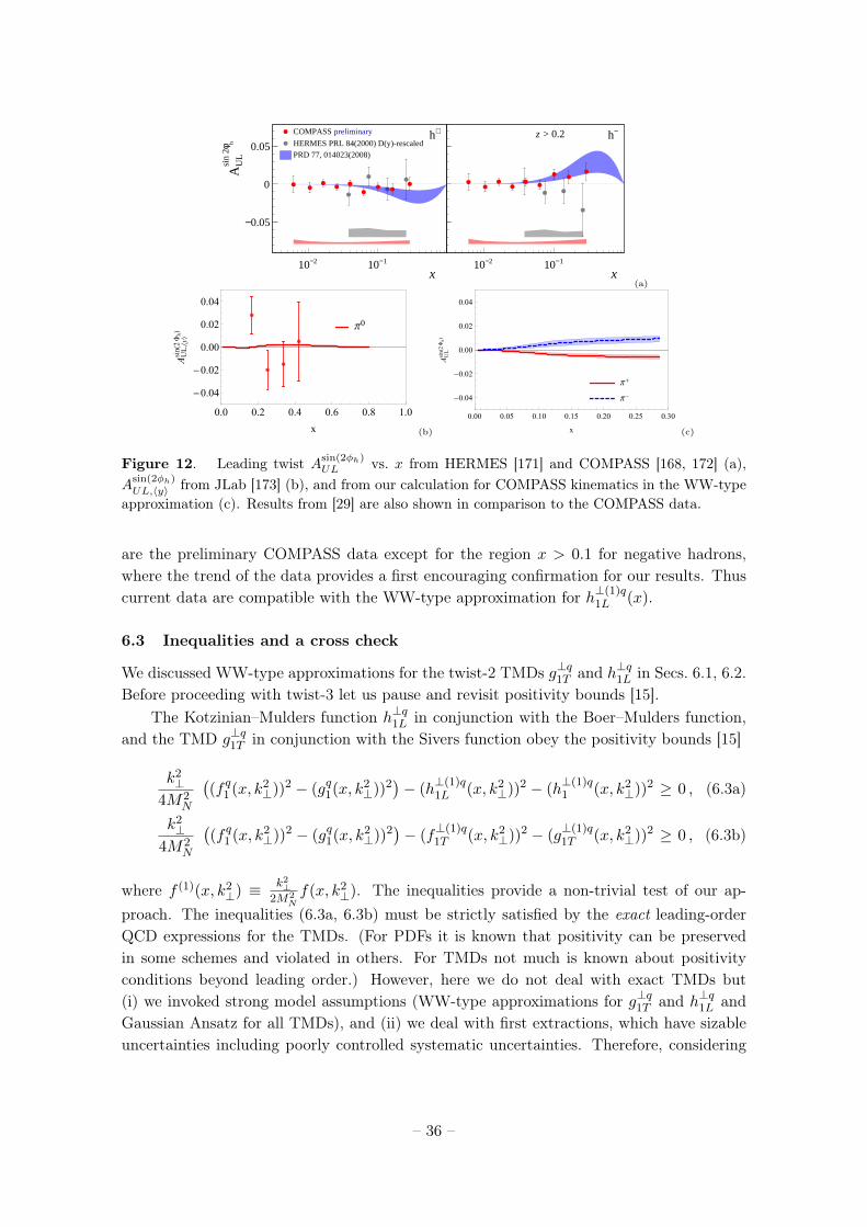
2−10 1−10
0.05−
0
0.05
+hpreliminaryCOMPASS
HERMES PRL 84(2000) D(y)-rescaledPRD 77, 014023(2008)
hφsi
n 2
UL
A
x2−10 1−10
0.05−
0
0.05
−h > 0.2z
x(a)
π0
0.0 0.2 0.4 0.6 0.8 1.0
-0.04
-0.02
0.00
0.02
0.04
x
AUL,⟨y⟩
sin(2Φh)
(b)
π+
π-
0.00 0.05 0.10 0.15 0.20 0.25 0.30
-0.04
-0.02
0.00
0.02
0.04
x
AULsin(2Φh)
(c)
Figure 12. Leading twist Asin(2φh)UL vs. x from HERMES [171] and COMPASS [168, 172] (a),
Asin(2φh)UL,〈y〉 from JLab [173] (b), and from our calculation for COMPASS kinematics in the WW-type
approximation (c). Results from [29] are also shown in comparison to the COMPASS data.
are the preliminary COMPASS data except for the region x > 0.1 for negative hadrons,where the trend of the data provides a first encouraging confirmation for our results. Thuscurrent data are compatible with the WW-type approximation for h⊥(1)q
1L (x).
6.3 Inequalities and a cross check
We discussed WW-type approximations for the twist-2 TMDs g⊥q1T and h⊥q1L in Secs. 6.1, 6.2.Before proceeding with twist-3 let us pause and revisit positivity bounds [15].
The Kotzinian–Mulders function h⊥q1L in conjunction with the Boer–Mulders function,and the TMD g⊥q1T in conjunction with the Sivers function obey the positivity bounds [15]
k2⊥
4M2N
((f q1 (x, k2
⊥))2 − (gq1(x, k2⊥))2
)− (h
⊥(1)q1L (x, k2
⊥))2 − (h⊥(1)q1 (x, k2
⊥))2 ≥ 0 , (6.3a)
k2⊥
4M2N
((f q1 (x, k2
⊥))2 − (gq1(x, k2⊥))2
)− (f
⊥(1)q1T (x, k2
⊥))2 − (g⊥(1)q1T (x, k2
⊥))2 ≥ 0 , (6.3b)
where f (1)(x, k2⊥) ≡ k2⊥
2M2Nf(x, k2
⊥). The inequalities provide a non-trivial test of our ap-proach. The inequalities (6.3a, 6.3b) must be strictly satisfied by the exact leading-orderQCD expressions for the TMDs. (For PDFs it is known that positivity can be preservedin some schemes and violated in others. For TMDs not much is known about positivityconditions beyond leading order.) However, here we do not deal with exact TMDs but(i) we invoked strong model assumptions (WW-type approximations for g⊥q1T and h⊥q1L andGaussian Ansatz for all TMDs), and (ii) we deal with first extractions, which have sizableuncertainties including poorly controlled systematic uncertainties. Therefore, considering
– 36 –
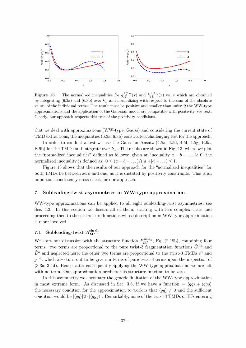
u
d
0.0 0.2 0.4 0.6 0.8 1.00.0
0.2
0.4
0.6
0.8
1.0
x
Positivityh 1L
⊥(1)q
u
d
0.0 0.2 0.4 0.6 0.8 1.0
0.0
0.2
0.4
0.6
0.8
1.0
x
Positivityg 1T
⊥(1)q
Figure 13. The normalized inequalities for g⊥(1)q1T (x) and h⊥(1)q1L (x) vs. x which are obtained
by integrating (6.3a) and (6.3b) over k⊥ and normalizing with respect to the sum of the absolutevalues of the individual terms. The result must be positive and smaller than unity if the WW-typeapproximations and the application of the Gaussian model are compatible with positivity, see text.Clearly, our approach respects this test of the positivity conditions.
that we deal with approximations (WW-type, Gauss) and considering the current state ofTMD extractions, the inequalities (6.3a, 6.3b) constitute a challenging test for the approach.
In order to conduct a test we use the Gaussian Ansatz (4.5a, 4.5d, 4.5f, 4.5g, B.9a,B.9b) for the TMDs and integrate over k⊥. The results are shown in Fig. 13, where we plotthe “normalized inequalities” defined as follows: given an inequality a − b − . . . ≥ 0, thenormalized inequality is defined as: 0 ≤ (a− b− . . . )/(|a|+|b|+ . . . ) ≤ 1.
Figure 13 shows that the results of our approach for the “normalized inequalities” forboth TMDs lie between zero and one, as it is dictated by positivity constraints. This is animportant consistency cross-check for our approach.
7 Subleading-twist asymmetries in WW-type approximation
WW-type approximations can be applied to all eight subleading-twist asymmetries, seeSec. 4.2. In this section we discuss all of them, starting with less complex cases andproceeding then to those structure functions whose description in WW-type approximationis more involved.
7.1 Subleading-twist AsinφhLU
We start our discussion with the structure function F sinφhLU , Eq. (2.19b), containing four
terms: two terms are proportional to the pure twist-3 fragmentation functions G⊥a andEa and neglected here; the other two terms are proportional to the twist-3 TMDs ea andg⊥a, which also turn out to be given in terms of pure twist-3 terms upon the inspection of(3.3a, 3.4d). Hence, after consequently applying the WW-type approximation, we are leftwith no term. Our approximation predicts this structure function to be zero.
In this asymmetry we encounter the generic limitation of the WW-type approximationin most extreme form. As discussed in Sec. 3.8, if we have a function = 〈qq〉 + 〈qgq〉the necessary condition for the approximation to work is that 〈qq〉 6= 0 and the sufficientcondition would be |〈qq〉|� |〈qgq〉|. Remarkably, none of the twist-3 TMDs or FFs entering
– 37 –
this structure function satisfy even the necessary condition. In this situation we do notexpect the WW-type approximation to work.
Indeed, data from COMPASS, HERMES, and JLab show a clearly non-zero asymmetryAsinφhLU = F sinφh
LU /FUU of the order of 2% [151, 175–179] (which includes the 1/Q factorintrinsic in twist-3 observables; without this factor the asymmetry would reach 10% atlarge x at COMPASS). This observable provides a unique opportunity to learn about thephysics of qgq-terms, but is beyond the applicability of the WW-type approximation.
With the numerator of the asymmetry proportional to qgq–terms and the denominatorgiven in terms of qq–terms, one could be tempted to interpret this observation as
AsinφhLU ∝ 〈qgq〉
〈qq〉exp∼ O(2 %) . (7.1)
Thus, in some sense the observed effect hints at the smallness of the involved qgq–terms.While in principle a correct observation, one should keep in mind several reservations.First, the experimental result (7.1) contains kinematic prefactors, which help to reducethe value. Second, the denominator contains fa1 and Da
1 , which are the largest TMD andFF because of positivity constraints. Third, the numerator is a sum of four terms, so itsoverall smallness could result from cancellation of different terms, rather than indicatingthat each single qgq–term is small. Fourth, some asymmetries predicted to be non-zero inWW-approximation are not much larger and in some cases even smaller than the result in(7.1).
To conclude, the WW-type approximation predicts AsinφLU ≈ 0 in contradiction to ex-
periment. The size of the observed effect seems in line with the WW-type approximation,as Asinφh
LU ∼ 〈qgq〉/〈qq〉 ∼ O(2 %) is not large, although this interpretation has reserva-tions. F sinφ
LU is the only twist-3 SIDIS structure function not “contaminated” by leadingtwist. Attempts to describe this observable and relevant model studies have been reported[34, 55, 94, 99–101, 180–189]. But more phenomenological work and dedicated studies onthe basis of models of qgq terms are needed to fully understand this asymmetry.
7.2 Subleading-twist AcosφS
LT
In the WW-type approximation the structure function F cosφSLT arises from gaT (x, k⊥) and
Da1(z, P⊥), whose collinear counterparts are more or less known, see Secs. 3.4 and 5.1. We
assume the Gaussian Ansatz for gaT (x, k⊥), shown in (B.9c) of App. B.3, with 〈k2⊥〉gT =
〈k2⊥〉g1 . We then determine gqT (x) according to (3.2a), which is a well-tested approximation
in DIS, see Sec. 3.4. In this way we obtain for F cosφSLT the result
F cosφSLT (x, z, PhT ) = −2MN
Qx2∑q
e2q g
qT (x)Dq
1(z) G(PhT ) , (7.2a)
F cosφSLT (x, z) = −2MN
Qx2∑q
e2q g
qT (x)Dq
1(z) , (7.2b)
with the width λ = z2〈k2⊥〉gT + 〈P 2
⊥〉D1 in the Gaussian G(PhT ).Notice that we followed here the scheme explained in Sec. 4.4: first assume Gaussian
Ansatz, then apply WW-type approximation. For some structure functions the order of
– 38 –
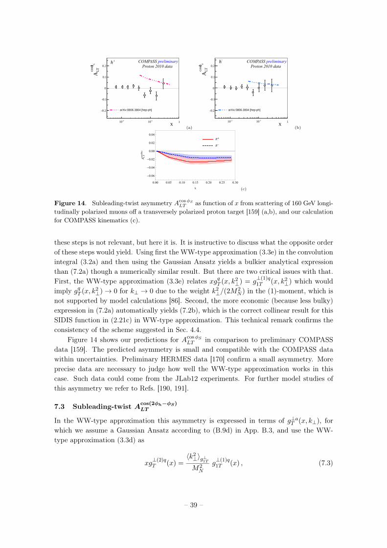
COMPASS preliminaryProton 2010 data
-210 -110 1
-0.2
-0.1
0
0.1
0.2h+
Sco
sϕ
LTA
x
arXiv:0806.3804 [hep-ph]
(a)
COMPASS preliminaryProton 2010 data
-210 -110 1
-0.2
-0.1
0
0.1
0.2
-h
Sco
sϕ
LTA
x
arXiv:0806.3804 [hep-ph]
(b)
π+
π-
0.00 0.05 0.10 0.15 0.20 0.25 0.30
-0.06
-0.04
-0.02
0.00
0.02
0.04
x
ALTcos(ΦS)
(c)
Figure 14. Subleading-twist asymmetry AcosφS
LT as function of x from scattering of 160 GeV longi-tudinally polarized muons off a transversely polarized proton target [159] (a,b), and our calculationfor COMPASS kinematics (c).
these steps is not relevant, but here it is. It is instructive to discuss what the opposite orderof these steps would yield. Using first the WW-type approximation (3.3e) in the convolutionintegral (3.2a) and then using the Gaussian Ansatz yields a bulkier analytical expressionthan (7.2a) though a numerically similar result. But there are two critical issues with that.First, the WW-type approximation (3.3e) relates xgqT (x, k2
⊥) = g⊥(1)q1T (x, k2
⊥) which wouldimply gqT (x, k2
⊥)→ 0 for k⊥ → 0 due to the weight k2⊥/(2M
2N ) in the (1)-moment, which is
not supported by model calculations [86]. Second, the more economic (because less bulky)expression in (7.2a) automatically yields (7.2b), which is the correct collinear result for thisSIDIS function in (2.21c) in WW-type approximation. This technical remark confirms theconsistency of the scheme suggested in Sec. 4.4.
Figure 14 shows our predictions for AcosφSLT in comparison to preliminary COMPASS
data [159]. The predicted asymmetry is small and compatible with the COMPASS datawithin uncertainties. Preliminary HERMES data [170] confirm a small asymmetry. Moreprecise data are necessary to judge how well the WW-type approximation works in thiscase. Such data could come from the JLab12 experiments. For further model studies ofthis asymmetry we refer to Refs. [190, 191].
7.3 Subleading-twist Acos(2φh−φS)LT
In the WW-type approximation this asymmetry is expressed in terms of g⊥aT (x, k⊥), forwhich we assume a Gaussian Ansatz according to (B.9d) in App. B.3, and use the WW-type approximation (3.3d) as
xg⊥(2)qT (x) =
〈k2⊥〉g⊥1TM2N
g⊥(1)q1T (x) , (7.3)
– 39 –
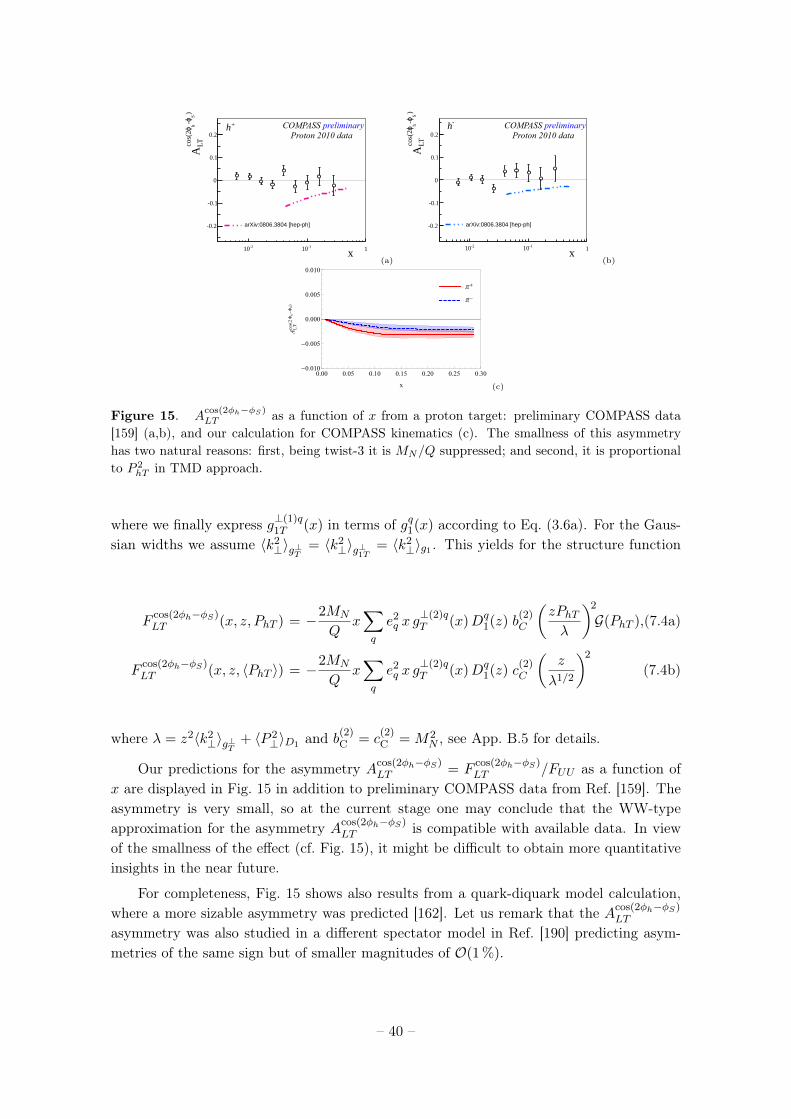
COMPASS preliminaryProton 2010 data
-210 -110 1
-0.2
-0.1
0
0.1
0.2h+
)S
-ϕh
cos(
2ϕLT
A
x
arXiv:0806.3804 [hep-ph]
(a)
COMPASS preliminaryProton 2010 data
-210 -110 1
-0.2
-0.1
0
0.1
0.2
-h
)S
-ϕh
cos(
2ϕLT
A
x
arXiv:0806.3804 [hep-ph]
(b)
π+
π-
0.00 0.05 0.10 0.15 0.20 0.25 0.30-0.010
-0.005
0.000
0.005
0.010
x
ALTcos(2Φh-ΦS)
(c)
Figure 15. Acos(2φh−φS)LT as a function of x from a proton target: preliminary COMPASS data
[159] (a,b), and our calculation for COMPASS kinematics (c). The smallness of this asymmetryhas two natural reasons: first, being twist-3 it is MN/Q suppressed; and second, it is proportionalto P 2
hT in TMD approach.
where we finally express g⊥(1)q1T (x) in terms of gq1(x) according to Eq. (3.6a). For the Gaus-
sian widths we assume 〈k2⊥〉g⊥T = 〈k2
⊥〉g⊥1T = 〈k2⊥〉g1 . This yields for the structure function
Fcos(2φh−φS)LT (x, z, PhT ) = −2MN
Qx∑q
e2q x g
⊥(2)qT (x)Dq
1(z) b(2)C
(zPhTλ
)2
G(PhT ),(7.4a)
Fcos(2φh−φS)LT (x, z, 〈PhT 〉) = −2MN
Qx∑q
e2q x g
⊥(2)qT (x)Dq
1(z) c(2)C
(z
λ1/2
)2
(7.4b)
where λ = z2〈k2⊥〉g⊥T + 〈P 2
⊥〉D1 and b(2)C = c
(2)C = M2
N , see App. B.5 for details.
Our predictions for the asymmetry Acos(2φh−φS)LT = F
cos(2φh−φS)LT /FUU as a function of
x are displayed in Fig. 15 in addition to preliminary COMPASS data from Ref. [159]. Theasymmetry is very small, so at the current stage one may conclude that the WW-typeapproximation for the asymmetry Acos(2φh−φS)
LT is compatible with available data. In viewof the smallness of the effect (cf. Fig. 15), it might be difficult to obtain more quantitativeinsights in the near future.
For completeness, Fig. 15 shows also results from a quark-diquark model calculation,where a more sizable asymmetry was predicted [162]. Let us remark that the Acos(2φh−φS)
LT
asymmetry was also studied in a different spectator model in Ref. [190] predicting asym-metries of the same sign but of smaller magnitudes of O(1 %).
– 40 –
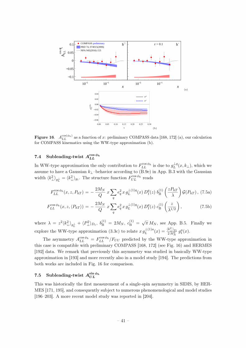
2−10 1−10
0.1−
0.05−
0
0.05
0.1 +hpreliminaryCOMPASS
PRD 74, 074015(2006)NPA 945(2016) 153
hφco
s
LL
A
x2−10 1−10
0.1−
0.05−
0
0.05
0.1 −h > 0.1z
x(a)
π+
π-
0.00 0.05 0.10 0.15 0.20 0.25 0.30
-0.06
-0.04
-0.02
0.00
0.02
0.04
x
ALLcos(Φh)
(b)
Figure 16. Acos(φh)LL as a function of x: preliminary COMPASS data [168, 172] (a), our calculation
for COMPASS kinematics using the WW-type approximation (b).
7.4 Subleading-twist AcosφhLL
In WW-type approximation the only contribution to F cosφhLL is due to g⊥qL (x, k⊥), which we
assume to have a Gaussian k⊥–behavior according to (B.9e) in App. B.3 with the Gaussianwidth 〈k2
⊥〉g⊥L = 〈k2⊥〉g1 . The structure function F cosφh
UL reads
F cosφhLL (x, z, PhT ) = − 2MN
Qx∑q
e2q x g
⊥(1)qL (x)Dq
1(z) b(1)B
(zPhTλ
)G(PhT ) , (7.5a)
F cosφhLL (x, z, 〈PhT 〉) = − 2MN
Qx∑q
e2q x g
⊥(1)qL (x)Dq
1(z) c(1)B
(z
λ1/2
), (7.5b)
where λ = z2〈k2⊥〉g⊥L + 〈P 2
⊥〉D1 , b(1)B = 2MN , c
(1)B =
√πMN , see App. B.5. Finally we
explore the WW-type approximation (3.3c) to relate x g⊥(1)aL (x) =
〈k2⊥〉g12M2
Nga1(x).
The asymmetry AcosφhLL = F cosφh
LL /FUU predicted by the WW-type approximation inthis case is compatible with preliminary COMPASS [168, 172] (see Fig. 16) and HERMES[192] data. We remark that previously this asymmetry was studied in basically WW-typeapproximation in [193] and more recently also in a model study [194]. The predictions fromboth works are included in Fig. 16 for comparison.
7.5 Subleading-twist AsinφhUL
This was historically the first measurement of a single-spin asymmetry in SIDIS, by HER-MES [171, 195], and consequently subject to numerous phenomenological and model studies[196–203]. A more recent model study was reported in [204].
– 41 –
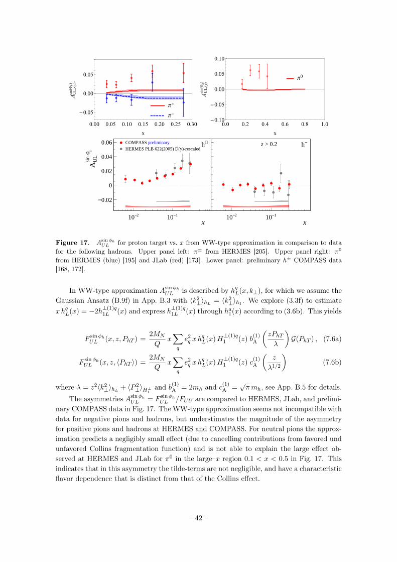
π+
π-
0.00 0.05 0.10 0.15 0.20 0.25 0.30
-0.05
0.00
0.05
x
AUL,<y>
sin(Φh)
π0
0.0 0.2 0.4 0.6 0.8 1.0-0.10
-0.05
0.00
0.05
0.10
x
AUL,⟨y⟩
sin(Φh)
2−10 1−10
0.02−
0
0.02
0.04
0.06 +hpreliminaryCOMPASS HERMES PLB 622(2005) D(y)-rescaledhφ
sin
UL
A
x2−10 1−10
0.02−
0
0.02
0.04
0.06 −h > 0.2z
x
Figure 17. Asinφh
UL for proton target vs. x from WW-type approximation in comparison to datafor the following hadrons. Upper panel left: π± from HERMES [205]. Upper panel right: π0
from HERMES (blue) [195] and JLab (red) [173]. Lower panel: preliminary h± COMPASS data[168, 172].
In WW-type approximation AsinφhUL is described by hqL(x, k⊥), for which we assume the
Gaussian Ansatz (B.9f) in App. B.3 with 〈k2⊥〉hL = 〈k2
⊥〉h1 . We explore (3.3f) to estimatexhqL(x) = −2h
⊥(1)q1L (x) and express h⊥(1)q
1L (x) through ha1(x) according to (3.6b). This yields
F sinφhUL (x, z, PhT ) =
2MN
Qx∑q
e2q xh
qL(x)H
⊥(1)q1 (z) b
(1)A
(zPhTλ
)G(PhT ) , (7.6a)
F sinφhUL (x, z, 〈PhT 〉) =
2MN
Qx∑q
e2q xh
qL(x)H
⊥(1)q1 (z) c
(1)A
(z
λ1/2
)(7.6b)
where λ = z2〈k2⊥〉hL + 〈P 2
⊥〉H⊥1 and b(1)A = 2mh and c(1)
A =√πmh, see App. B.5 for details.
The asymmetries AsinφhUL = F sinφh
UL /FUU are compared to HERMES, JLab, and prelimi-nary COMPASS data in Fig. 17. The WW-type approximation seems not incompatible withdata for negative pions and hadrons, but understimates the magnitude of the asymmetryfor positive pions and hadrons at HERMES and COMPASS. For neutral pions the approx-imation predicts a negligibly small effect (due to cancelling contributions from favored undunfavored Collins fragmentation function) and is not able to explain the large effect ob-served at HERMES and JLab for π0 in the large–x region 0.1 < x < 0.5 in Fig. 17. Thisindicates that in this asymmetry the tilde-terms are not negligible, and have a characteristicflavor dependence that is distinct from that of the Collins effect.
– 42 –
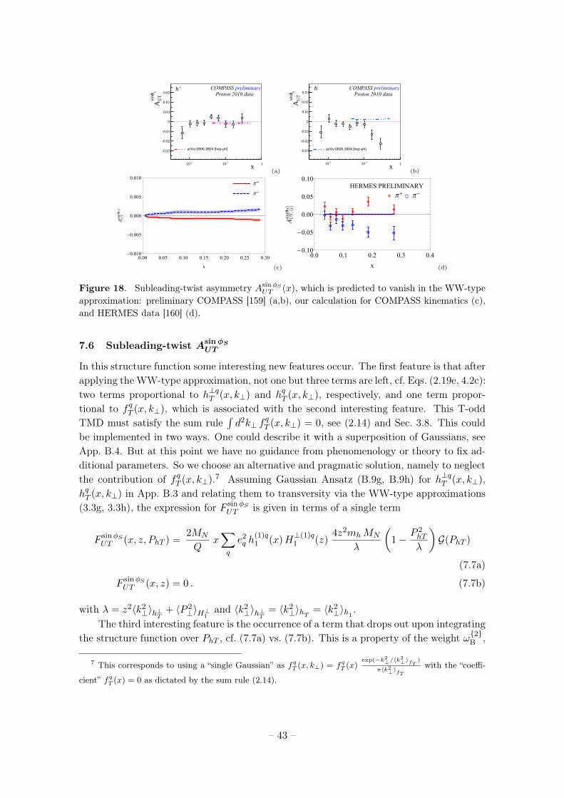
COMPASS preliminaryProton 2010 data
-210 -110 1
-0.03
-0.02
-0.01
0
0.01
0.02
0.03h+
Ssi
nϕ
UT
A
x
arXiv:0806.3804 [hep-ph]
(a)
COMPASS preliminaryProton 2010 data
-210 -110 1
-0.03
-0.02
-0.01
0
0.01
0.02
0.03
-h
Ssi
nϕ
UT
A
x
arXiv:0806.3804 [hep-ph]
(b)
π+
π-
0.00 0.05 0.10 0.15 0.20 0.25 0.30-0.010
-0.005
0.000
0.005
0.010
x
AUTsin(ΦS)
(c)
HERMES PRELIMINARY
π+ π-
0.0 0.1 0.2 0.3 0.4-0.10
-0.05
0.00
0.05
0.10
x
AUT,⟨y⟩
sin(ΦS)
(d)
Figure 18. Subleading-twist asymmetry AsinφS
UT (x), which is predicted to vanish in the WW-typeapproximation: preliminary COMPASS [159] (a,b), our calculation for COMPASS kinematics (c),and HERMES data [160] (d).
7.6 Subleading-twist AsinφS
UT
In this structure function some interesting new features occur. The first feature is that afterapplying theWW-type approximation, not one but three terms are left, cf. Eqs. (2.19e, 4.2c):two terms proportional to h⊥qT (x, k⊥) and hqT (x, k⊥), respectively, and one term propor-tional to f qT (x, k⊥), which is associated with the second interesting feature. This T-oddTMD must satisfy the sum rule
∫d2k⊥ f
qT (x, k⊥) = 0, see (2.14) and Sec. 3.8. This could
be implemented in two ways. One could describe it with a superposition of Gaussians, seeApp. B.4. But at this point we have no guidance from phenomenology or theory to fix ad-ditional parameters. So we choose an alternative and pragmatic solution, namely to neglectthe contribution of f qT (x, k⊥).7 Assuming Gaussian Ansatz (B.9g, B.9h) for h⊥qT (x, k⊥),hqT (x, k⊥) in App. B.3 and relating them to transversity via the WW-type approximations(3.3g, 3.3h), the expression for F sinφS
UT is given in terms of a single term
F sinφSUT (x, z, PhT ) =
2MN
Qx∑q
e2q h
(1)q1 (x)H
⊥(1)q1 (z)
4z2mhMN
λ
(1−
P 2hT
λ
)G(PhT )
(7.7a)
F sinφSUT (x, z) = 0 . (7.7b)
with λ = z2〈k2⊥〉h⊥T + 〈P 2
⊥〉H⊥1 and 〈k2⊥〉h⊥T = 〈k2
⊥〉hT = 〈k2⊥〉h1 .
The third interesting feature is the occurrence of a term that drops out upon integratingthe structure function over PhT , cf. (7.7a) vs. (7.7b). This is a property of the weight ω{2}B ,
7 This corresponds to using a “single Gaussian” as fqT (x, k⊥) = fqT (x)exp(−k2⊥/〈k
2⊥〉fT )
π〈k2⊥〉fTwith the “coeffi-
cient” fqT (x) = 0 as dictated by the sum rule (2.14).
– 43 –
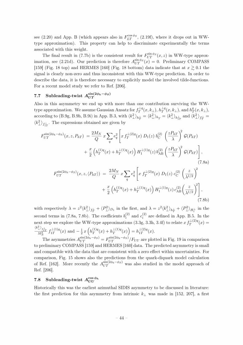
see (2.20) and App. B (which appears also in F cosφSLT , (2.19f), where it drops out in WW-
type approximation). This property can help to discriminate experimentally the termsassociated with this weight.
The final result in (7.7b) is the consistent result for F sinφSUT (x, z) in WW-type approx-
imation, see (2.21d). Our prediction is therefore AsinφSUT (x) = 0. Preliminary COMPASS
[159] (Fig. 18 top) and HERMES [160] (Fig. 18 bottom) data indicate that at x & 0.1 thesignal is clearly non-zero and thus inconsistent with this WW-type prediction. In order todescribe the data, it is therefore necessary to explicitly model the involved tilde-functions.For a recent model study we refer to Ref. [206].
7.7 Subleading-twist Asin(2φh−φS)UT
Also in this asymmetry we end up with more than one contribution surviving the WW-type approximation. We assume Gaussian Ansatz for f⊥qT (x, k⊥), h⊥qT (x, k⊥), and hqT (x, k⊥),according to (B.9g, B.9h, B.9i) in App. B.3, with 〈k2
⊥〉h⊥T = 〈k2⊥〉hT = 〈k2
⊥〉h⊥1T and 〈k2⊥〉f⊥T =
〈k2⊥〉f⊥1T . The expressions obtained are given by
Fsin(2φh−φS)UT (x, z, PhT ) =
2MN
Qx∑q
e2q
[x f⊥(2)qT (x) D1(z) b
(2)C
(zPhTλ
)2
G(PhT )
+x
2
(h
(1)qT (x) + h
⊥(1)qT (x)
)H⊥(1)q1 (z) b
(2)AB
(zPhTλ
)2
G(PhT )
],
(7.8a)
Fsin(2φh−φS)UT (x, z, 〈PhT 〉) =
2MN
Qx∑q
e2q
[x f⊥(2)qT (x) D1(z) c
(2)C
(z
λ1/2
)2
+x
2
(h
(1)qT (x) + h
⊥(1)qT (x)
)H⊥(1)q1 (z) c
(2)AB
(z
λ1/2
)2],
(7.8b)
with respectively λ = z2〈k2⊥〉f⊥T + 〈P 2
⊥〉D1 in the first, and λ = z2〈k2⊥〉h⊥T + 〈P 2
⊥〉H⊥1 in the
second terms in (7.8a, 7.8b). The coefficients b(2)i and c(2)
i are defined in App. B.5. In thenext step we explore the WW-type approximations (3.3g, 3.3h, 3.4f) to relate x f⊥(2)q
T (x) =〈k2⊥〉f⊥
1T
M2N
f⊥(1)q1T (x) and − 1
2 x(h
(1)qT (x) + h
⊥(1)qT (x)
)= h
⊥(2)q1T (x).
The asymmetries Asin(2φh−φS)UT = F
sin(2φh−φS)UT /FUU are plotted in Fig. 19 in comparison
to preliminary COMPASS [159] and HERMES [160] data. The predicted asymmetry is smalland compatible with the data that are consistent with a zero effect within uncertainties. Forcomparison, Fig. 15 shows also the predictions from the quark-diquark model calculationof Ref. [162]. More recently the Asin(2φh−φS)
UT was also studied in the model approach ofRef. [206].
7.8 Subleading-twist AcosφhUU
Historically this was the earliest azimuthal SIDIS asymmetry to be discussed in literature:the first prediction for this asymmetry from intrinsic k⊥ was made in [152, 207], a first
– 44 –
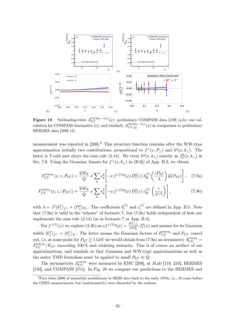
COMPASS preliminaryProton 2010 data
-210 -110 1
-0.03
-0.02
-0.01
0
0.01
0.02
0.03h+
)S
-ϕh
sin(
2ϕ
UT
Ax
arXiv:0806.3804 [hep-ph]
(a)
COMPASS preliminaryProton 2010 data
-210 -110 1
-0.03
-0.02
-0.01
0
0.01
0.02
0.03h+
)S
-ϕh
sin(
2ϕ
UT
A
x
arXiv:0806.3804 [hep-ph]
(b)
π+
π-
0.00 0.05 0.10 0.15 0.20 0.25 0.30-0.02
-0.01
0.00
0.01
0.02
x
AUTsin(2Φh-ΦS)
(c)
HERMES PRELIMINARY
π+ π-
0.0 0.1 0.2 0.3 0.4
-0.04
-0.02
0.00
0.02
0.04
x
AUT,⟨y⟩
sin(2Φh-ΦS)
(d)
Figure 19. Subleading-twist Asin(2φh−φS)UT (x): preliminary COMPASS data [159] (a,b), our cal-
culation for COMPASS kinematics (c), and similarly Asin(2φh−φS)UT,〈y〉 (x) in comparison to preliminary
HERMES data [160] (d).
measurement was reported in [208].8 This structure function contains after the WW-typeapproximation initially two contributions, proportional to f⊥(x, P⊥) and hq(x, k⊥). Thelatter is T-odd and obeys the sum rule (2.14). We treat hq(x, k⊥) exactly as f qT (x, k⊥) inSec. 7.6. Using the Gaussian Ansatz for f⊥(x, k⊥) in (B.9j) of App. B.3, we obtain
F cosφhUU (x, z, PhT ) =
2MN
Qx∑q
e2q
[−x f⊥(1)q(x)Dq
1(z) b(1)B
(zPhTλ
)G(PhT )
], (7.9a)
F cosφhUU (x, z, 〈PhT 〉) =
2MN
Qx∑q
e2q
[−x f⊥(1)q(x)Dq
1(z) c(1)B
(z
λ1/2
)], (7.9b)
with λ = z2〈k2⊥〉f⊥ + 〈P 2
⊥〉D1 . The coefficients b(1)i and c(1)
i are defined in App. B.5. Notethat (7.9a) is valid in the “scheme” of footnote 7, but (7.9a) holds independent of how oneimplements the sum rule (2.14) (as in footnote 7 or App. B.4).
For f⊥(1)(x) we explore (3.3b) as xf⊥(1)q(x) =〈k2⊥〉f12M2
Nf q1 (x) and assume for its Gaussian
width 〈k2⊥〉f⊥ = 〈k2
⊥〉f1 . The latter means the Gaussian factors of F cosφhUU and FUU cancel
out, i.e. at some point for PhT & 1GeV we would obtain from (7.9a) an asymmetry AcosφhUU =
F cosφhUU /FUU exceeding 100% and violating unitarity. This is of course an artifact of our
approximations, and reminds us that Gaussian and WW-type approximations as well asthe entire TMD formalism must be applied to small PhT � Q.
The asymmetries AcosφhUU were measured by EMC [208], at JLab [119, 210], HERMES
[150], and COMPASS [151]. In Fig. 20 we compare our predictions to the HERMES and
8First hints [209] of azimuthal modulations in SIDIS date back to the early 1970s, i.e., 10 years beforethe CERN measurements, but (unfortunately) were discarded by the authors.
– 45 –
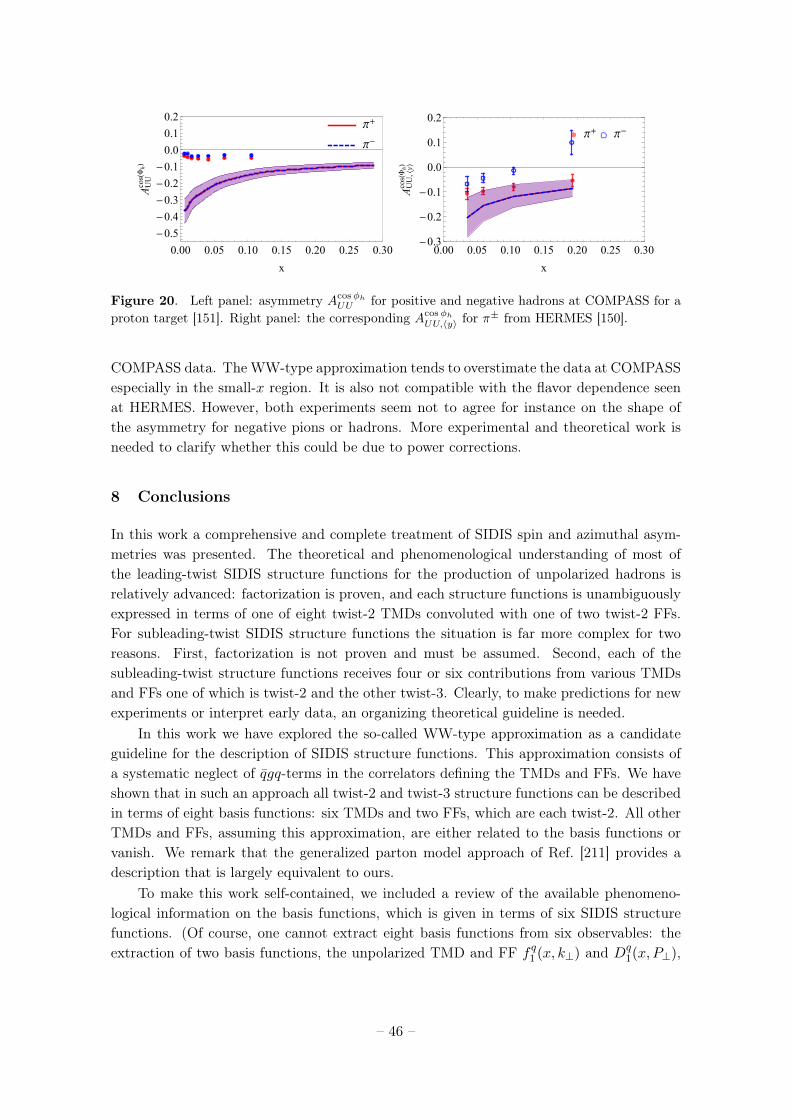
π+
π-
0.00 0.05 0.10 0.15 0.20 0.25 0.30
-0.5
-0.4
-0.3
-0.2
-0.1
0.0
0.1
0.2
x
AUUcos(Φh)
π+ π-
0.00 0.05 0.10 0.15 0.20 0.25 0.30-0.3
-0.2
-0.1
0.0
0.1
0.2
x
AUU,⟨y⟩
cos(Φh)
Figure 20. Left panel: asymmetry Acosφh
UU for positive and negative hadrons at COMPASS for aproton target [151]. Right panel: the corresponding Acosφh
UU,〈y〉 for π± from HERMES [150].
COMPASS data. TheWW-type approximation tends to overstimate the data at COMPASSespecially in the small-x region. It is also not compatible with the flavor dependence seenat HERMES. However, both experiments seem not to agree for instance on the shape ofthe asymmetry for negative pions or hadrons. More experimental and theoretical work isneeded to clarify whether this could be due to power corrections.
8 Conclusions
In this work a comprehensive and complete treatment of SIDIS spin and azimuthal asym-metries was presented. The theoretical and phenomenological understanding of most ofthe leading-twist SIDIS structure functions for the production of unpolarized hadrons isrelatively advanced: factorization is proven, and each structure functions is unambiguouslyexpressed in terms of one of eight twist-2 TMDs convoluted with one of two twist-2 FFs.For subleading-twist SIDIS structure functions the situation is far more complex for tworeasons. First, factorization is not proven and must be assumed. Second, each of thesubleading-twist structure functions receives four or six contributions from various TMDsand FFs one of which is twist-2 and the other twist-3. Clearly, to make predictions for newexperiments or interpret early data, an organizing theoretical guideline is needed.
In this work we have explored the so-called WW-type approximation as a candidateguideline for the description of SIDIS structure functions. This approximation consists ofa systematic neglect of qgq-terms in the correlators defining the TMDs and FFs. We haveshown that in such an approach all twist-2 and twist-3 structure functions can be describedin terms of eight basis functions: six TMDs and two FFs, which are each twist-2. All otherTMDs and FFs, assuming this approximation, are either related to the basis functions orvanish. We remark that the generalized parton model approach of Ref. [211] provides adescription that is largely equivalent to ours.
To make this work self-contained, we included a review of the available phenomeno-logical information on the basis functions, which is given in terms of six SIDIS structurefunctions. (Of course, one cannot extract eight basis functions from six observables: theextraction of two basis functions, the unpolarized TMD and FF f q1 (x, k⊥) and Dq
1(x, P⊥),
– 46 –
makes also use of other experiments, most notably Drell–Yan and hadron production ine+e− annihilations.)
The WW-type approximation for TMDs and FFs is inspired by the observation that theclassical WW-approximation for the twist-3 DIS structure function g2(x) (or PDF gqT (x))works well. This was predicted in theoretical studies in the instanton model of the QCDvacuum, and confirmed by data and lattice QCD studies. The classic WW approximationfor g2(x) works with a relative accuracy of ± 40 % or better. This is remarkable. The instan-ton vacuum model predicts an analogous WW approximation for the chirally odd twist-3PDF hqL(x) to work similarly well. This prediction remains to be tested in experiment.
In each case, gqT (x) and hqL(x), we deal with nucleon matrix elements of different qgqcorrelators, which are assumed to be small. Can one generalize these approximations toTMDs? This is a key question, which has been addressed in the past in literature in selectedcases. This work is the first systematic investigation of this question. As in the unintegratedcorrelators one deals with different classes of operators, we prefer to speak of the WW-typeapproximation to distinguish from the collinear case.
We have studied in detail all SIDIS structure function in this approximation. Thisincludes a review of results from lattice QCD calculations, effective theories and models.We found that from theoretical point of view the WW-type approximations receive certainsupport, though there is less evidence than in the collinear case. Most importantly, we haveconducted systematic tests of WW approximations with available published or preliminary(and soon to be published) SIDIS data from HERMES, COMPASS, and JLab.
We found the following results. The two leading-twist structure functions amenable toWW-type approximations, F cos(φh−φS)
LT and F sin(2φh)UL , are well-described (the former) or at
least compatible (the latter) with the data in this approximation. For F sin(2φh)UL more precise
data are needed, but also in this case the trend is encouraging especially thanks to the recentpreliminary COMPASS data. We have also shown that our approach satisfies positivityinequalities, which is a non-trivial consistency check considering the crude approximations(WW-type, Gaussian Ansatz for TMDs) in our approach.
At subleading twist the WW-type approximation for the structure functions F cosφSLT ,
Fcos(2φh−φS)LT , F cosφh
LL , F sin(2φh−φS)UT is compatible with data, too. Some of these asymmetries
are predicted to be very small in the WW-type approximation, sometimes smaller thana fraction of a percent. This is compatible with the available data in the sense that thedata are consistent with zero within their statistical accuracies. This cannot be considered athorough evidence for the applicability of the WW-type approximations, but on the positivesite we also observe no alarming hints that the WW-type approximations fail in these cases.
In the case of the three subleading-twist structure functions F cosφhUU , F sinφh
UL , F sinφhLU ,
and F sinφSUT the situation is clearer and indicates that here the WW-type approximations
do not work. Incidentally, these asymmetries include the very first non-zero azimuthalasymmetry measured in unpolarized SIDIS (F cosφh
UU ), the very first non-zero target single-spin asymmetry measured in SIDIS (F sinφh
UL ), and and the beam-spin asymmetry (F sinφhLU ).
The WW-type prediction for F cos(φh)UU tends to overshoot the data. In the case of F sinφh
UL
the WW-type approximation undershoots data by a factor of 2 or so. Most interestingly,
– 47 –
in the case of F sinφhLU the WW-type approximation predicts exactly a zero asymmetry, but
experiments see small but non-zero effect.The non-applicability of the WW–type approximation in these three cases should not be
too surprising. After all it is a crude method to model TMDs and FFs and an uncontrollable“expansion” (in nuclear physics the concept of 2–body, 3–body, etc operators is well-justifiedand an effective expansion can be conducted; in the case of TMDs, however, it is lessappropriate to speak about a systematic expansion in terms of qq, qgq, etc correlators).It will be very interesting to learn whether, e.g., in F sinφh
UL or F sinφhLU a single qgq–term is
anomalously large, or whether it is a accumulative effect of several small terms qgq–termsadding up to the observed asymmetry.
Among all SIDIS structure functions F sinφhLU emerges as a particularly interesting case:
this asymmetry is due to qgq only, without “contamination” from qq terms. Thus F sinφhLU
offers a unique view on the physics of qgq correlators, worth exploring for its own sake.The results presented in this work are of importance for several reasons. To the best of
our knowledge, it is the first complete study of all SIDIS structure functions up to twist-3in a unique approach. The results are useful for experiments prepared in the near term(JLab 12) or proposed in the long term (Electron-Ion Collider), and provide helpful inputfor Monte Carlo event generators [33]. Our predictions will help to pave the way towards abetter understanding of the quark-gluon structure of the nucleon beyond leading twist.
9 Acknowledgments
First and foremost, the authors would like to thank their families for patience and constantsupport throughout writing this paper. The authors would like to thank Werner Vogelsangfor many useful discussions. This work was partially supported by the U.S. Department ofEnergy under Contract No. DE-AC05-06OR23177 (A.P.) and within the TMD Collabora-tion framework, and by the National Science Foundation under Contract No. PHY-1623454(A.P.) and Contract No. PHY-1406298 (P.S.), and the Wilhelm Schuler Stiftung (P.S.).
A The “minimal basis” of TMDs and FFs
This Appendix describes the technical details of the parametrizations used in this work.
A.1 Unpolarized functions fa1 (x, k2⊥) and D
a1(z, P
2⊥)
In this work we use the leading-order parametrizations from [115] for the unpolarized PDFfa1 (x) and from [116] for the unpolarized FF Da
1(z). If not otherwise stated the parametriza-tions are taken at the scale Q2 = 2.4 GeV2 typical for many currently available SIDIS data.These parametrizations were used in [107] and other works whose extractions we adopt.
To describe the transverse momentum dependence of fa1 (x, k2⊥) and D1(z, P 2
⊥) we usethe Gaussian Ansatz in Eqs. (4.5a, 4.5b). All early [107–110] and some recent [111] analysesemployed flavor and x– or z–independent widths 〈k2
⊥〉 and 〈P 2⊥〉. In the analysis [112] of
HERMES multiplicities flavor-independence of the widths was assumed. On long run onemay anticipate that new precision data will require to relax these assumptions. However,
– 48 –
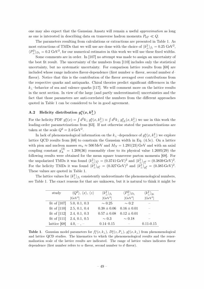
one may also expect that the Gaussian Ansatz will remain a useful approximation as longas one is interested in describing data on transverse hadron momenta PhT � Q.
The parameters resulting from calculations or extractions are presented in Table 1. Asmost extractions of TMDs that we will use are done with the choice of 〈k2
⊥〉f1 = 0.25 GeV2,〈P 2⊥〉D1 = 0.2 GeV2, for our numerical estimates in this work we will use these fixed widths.Some comments are in order. In [107] no attempt was made to assign an uncertainty of
the best fit result. The uncertainty of the numbers from [110] includes only the statisticaluncertainty, but no systematic uncertainty. For comparison lattice results from [68] areincluded whose range indicates flavor-dependence (first number u–flavor, second number d–flavor). Notice that this is the contribution of the flavor averaged over contributions fromthe respective quarks and antiquarks. Chiral theories predict significant differences in thek⊥–behavior of sea and valence quarks [117]. We will comment more on the lattice resultsin the next section. In view of the large (and partly underestimated) uncertainties and thefact that those parameters are anti-correlated the numbers from the different approachesquoted in Table 1 can be considered to be in good agreement.
A.2 Helicity distribution ga1(x, k2⊥)
For the helicity PDF ga1(x) =∫d2k⊥ g
a1(x, k2
⊥) ≡∫d2k⊥ g
a1L(x, k2
⊥) we use in this work theleading-order parametrizations from [63]. If not otherwise stated the parametrizations aretaken at the scale Q2 = 2.4 GeV2.
In lack of phenomenological information on the k⊥–dependence of ga1(x, k2⊥) we explore
lattice QCD results from [68] to constrain the Gaussian width in Eq. (4.5c). On a latticewith pion and nucleon masses mπ ≈ 500 MeV and MN = 1.291(23) GeV and with an axialcoupling constant g(3)
A = 1.209(36) reasonably close to its physical value 1.2695(29) thefollowing results were obtained for the mean square transverse parton momenta [68]. Forthe unpolarized TMDs it was found 〈k2
⊥〉fu1 = (0.3741 GeV)2 and 〈k2⊥〉fd1 = (0.3839 GeV)2.
For the helicity TMDs it was found 〈k2⊥〉gu1 = (0.327 GeV)2 and 〈k2
⊥〉gd1 = (0.385 GeV)2.These values are quoted in Table 1.
The lattice values for 〈k2⊥〉f1 consistently underestimate the phenomenological numbers,
see Table 1. The exact reasons for that are unknown, but it is natural to think it might be
study 〈Q2〉, 〈x〉, 〈z〉 〈k2⊥〉f1 〈P 2
⊥〉D1 〈k2⊥〉g1
[GeV2] [GeV2] [GeV2] [GeV2]
fit of [107] 5.0, 0.1, 0.3 ∼ 0.25 ∼ 0.2 –fit of [110] 2.5, 0.1, 0.4 0.38± 0.06 0.16± 0.01 –fit of [112] 2.4, 0.1, 0.3 0.57± 0.08 0.12± 0.01 –fit of [111] 2.4, 0.1, 0.5 ∼ 0.3 ∼ 0.18 –lattice [68] 4.0, – , – 0.14–0.15 – 0.11-0.15
Table 1. Gaussian model parameters for fa1 (x, k⊥), Da1(z, P⊥), ga1 (x, k⊥) from phenomenological
and lattice QCD studies. The kinematics to which the phenomenological results and the renor-malization scale of the lattice results are indicated. The range of lattice values indicates flavordependence (first number refers to u–flavor, second number to d–flavor).
– 49 –
related to the fact that the lattice predictions [68] do not refer to TMDs entering in SIDIS (orDrell–Yan or other process) because a different gauge link was chosen, see Sec. 3.5. Still onemay expect these results to bear considerable information on QCD dynamics.9 To make useof this information we shall assume that the lattice results [68] provide robust predictionsfor the ratios 〈k2
⊥〉gu1 /〈k2⊥〉fu1 ≈ 0.76. With the phenomenological value 〈k2
⊥〉f1 = 0.25 GeV2
we then obtain the estimate for the width of the helicity TMD 〈k2⊥〉g1 = 0.19 GeV2. In our
phenomenological study we use this value for u–quarks and for simplicity also for d–quarks.Even though the lattice values indicate an interesting flavor dependence, see Table 1, for aproton target this is a very good approximation due to u–quark dominance. When precisiondata for deuterium and especially for 3He from JLab become available, it will be interestingto re-investigate this point in detail.
A.3 Sivers function f⊥q1T (x, k⊥)
Sivers distribution function was studied in Refs. [45, 46, 124, 132–134, 211–214]. We willuse parametrizations from Refs. [124, 132, 211]:
〈k2⊥〉f⊥1T ≡
〈k2⊥〉M2
1
〈k2⊥〉+M2
1
(A.1)
f⊥1T (x, k2⊥) = −M
M1
√2e Nq(x) fq/p(x,Q)
e−k2⊥/〈k
2⊥〉f⊥
1T
π〈k2⊥〉
, (A.2)
where M1 is a mass parameter, M the proton mass and
Nq(x) = Nq xα(1− x)β
(α+ β)(α+β)
ααββ(A.3)
The first moment of Sivers function is:
f⊥(1)q1T (x) = −
√e2 〈k
2⊥〉M3
1
M(〈k2⊥〉+M2
1 )2Nq(x)fq(x,Q) = −
√e
2
1
MM1
〈k2⊥〉2f⊥1T〈k2⊥〉
Nq(x)fq(x,Q) .(A.4)
We can rewrite parametrizations of Sivers functions as
f⊥q1T (x, k2⊥) = f
⊥(1)q1T (x)
2M2
π〈k2⊥〉2f⊥1T
e−k2⊥/〈k
2⊥〉f⊥
1T . (A.5)
The fit the HERMES proton and COMPASS deuteron data from including only Siversfunctions for u and d quarks was done in Ref. [124], corresponding to seven free parameters,and parameters are shown in Table 2.
9 The results [68] refer also to pion masses above the physical value. This caveat is presumably lesscritical and will be overcome as lattice QCD simulations are becoming feasible at physical pion masses.
– 50 –
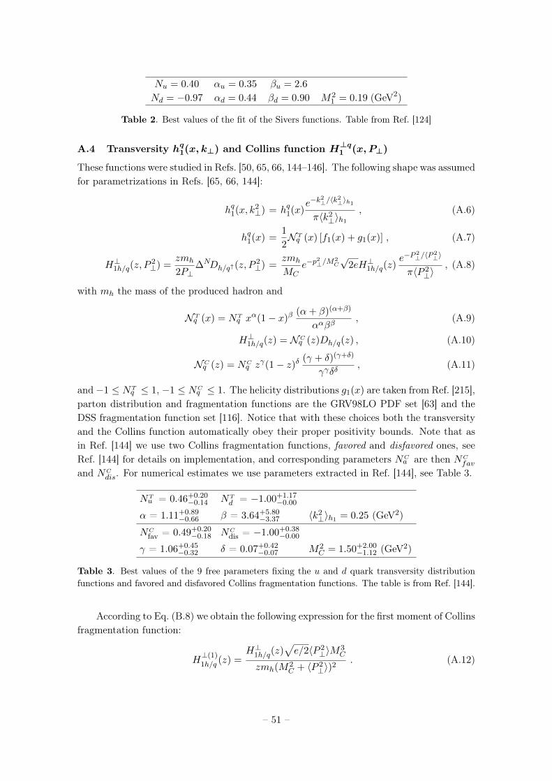
Nu = 0.40 αu = 0.35 βu = 2.6
Nd = −0.97 αd = 0.44 βd = 0.90 M21 = 0.19 (GeV2)
Table 2. Best values of the fit of the Sivers functions. Table from Ref. [124]
A.4 Transversity hq1(x, k⊥) and Collins function H⊥q1 (x, P⊥)
These functions were studied in Refs. [50, 65, 66, 144–146]. The following shape was assumedfor parametrizations in Refs. [65, 66, 144]:
hq1(x, k2⊥) = hq1(x)
e−k2⊥/〈k
2⊥〉h1
π〈k2⊥〉h1
, (A.6)
hq1(x) =1
2N Tq (x) [f1(x) + g1(x)] , (A.7)
H⊥1h/q(z, P2⊥) =
zmh
2P⊥∆NDh/q↑(z, P
2⊥) =
zmh
MCe−p
2⊥/M
2C
√2eH⊥1h/q(z)
e−P2⊥/〈P
2⊥〉
π〈P 2⊥〉
, (A.8)
with mh the mass of the produced hadron and
N Tq (x) = NT
q xα(1− x)β
(α+ β)(α+β)
ααββ, (A.9)
H⊥1h/q(z) = N Cq (z)Dh/q(z) , (A.10)
N Cq (z) = NC
q zγ(1− z)δ (γ + δ)(γ+δ)
γγδδ, (A.11)
and−1 ≤ NTq ≤ 1, −1 ≤ NC
q ≤ 1. The helicity distributions g1(x) are taken from Ref. [215],parton distribution and fragmentation functions are the GRV98LO PDF set [63] and theDSS fragmentation function set [116]. Notice that with these choices both the transversityand the Collins function automatically obey their proper positivity bounds. Note that asin Ref. [144] we use two Collins fragmentation functions, favored and disfavored ones, seeRef. [144] for details on implementation, and corresponding parameters NC
a are then NCfav
and NCdis. For numerical estimates we use parameters extracted in Ref. [144], see Table 3.
NTu = 0.46+0.20
−0.14 NTd = −1.00+1.17
−0.00
α = 1.11+0.89−0.66 β = 3.64+5.80
−3.37 〈k2⊥〉h1 = 0.25 (GeV2)
NCfav = 0.49+0.20
−0.18 NCdis = −1.00+0.38
−0.00
γ = 1.06+0.45−0.32 δ = 0.07+0.42
−0.07 M2C = 1.50+2.00
−1.12 (GeV2)
Table 3. Best values of the 9 free parameters fixing the u and d quark transversity distributionfunctions and favored and disfavored Collins fragmentation functions. The table is from Ref. [144].
According to Eq. (B.8) we obtain the following expression for the first moment of Collinsfragmentation function:
H⊥(1)1h/q (z) =
H⊥1h/q(z)√e/2〈P 2
⊥〉M3C
zmh(M2C + 〈P 2
⊥〉)2. (A.12)
– 51 –
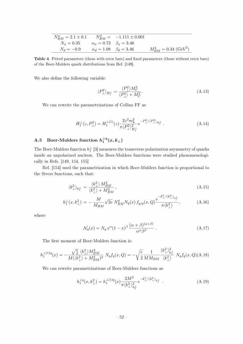
NuBM = 2.1± 0.1 Nd
BM = −1.111± 0.001
Nu = 0.35 αu = 0.73 βu = 3.46
Nd = −0.9 αd = 1.08 βd = 3.46 M2BM = 0.34 (GeV2)
Table 4. Fitted parameters (those with error bars) and fixed parameters (those without error bars)of the Boer-Mulders quark distributions from Ref. [149].
We also define the following variable:
〈P 2⊥〉H⊥1 =
〈P 2⊥〉M2
C
〈P 2⊥〉+M2
C
. (A.13)
We can rewrite the parametrizations of Collins FF as
H⊥1 (z, P 2⊥) = H
⊥(1)1 (z)
2z2m2h
π〈P 2⊥〉2H⊥1
e−P 2⊥/〈P
2⊥〉H⊥1 . (A.14)
A.5 Boer-Mulders function h⊥q1 (x, k⊥)
The Boer-Mulders function h⊥1 [3] measures the transverse polarization asymmetry of quarksinside an unpolarized nucleon. The Boer-Mulders functions were studied phenomenologi-cally in Refs. [149, 154, 155]
Ref. [154] used the parametrization in which Boer-Mulders function is proportional tothe Sivers functions, such that:
〈k2⊥〉h⊥1 =
〈k2⊥〉M2
BM
〈k2⊥〉+M2
BM
, (A.15)
h⊥1 (x, k2⊥) = − M
MBM
√2e N q
BMNq(x) fq/p(x,Q)e−k2⊥/〈k
2⊥〉h⊥1
π〈k2⊥〉
, (A.16)
where
Nq(x) = Nq xα(1− x)β
(α+ β)(α+β)
ααββ. (A.17)
The first moment of Boer-Mulders function is:
h⊥(1)q1 (x) = −
√e2 〈k
2⊥〉M3
BM
M(〈k2⊥〉+M2
BM )2Nqfq(x,Q) = −
√e
2
1
MMBM
〈k2⊥〉2h⊥1〈k2⊥〉
Nqfq(x,Q) .(A.18)
We can rewrite parametrizations of Boer-Mulders functions as
h⊥q1 (x, k2⊥) = h
⊥(1)q1 (x)
2M2
π〈k2⊥〉2h⊥1
e−k2⊥/〈k
2⊥〉h⊥1 . (A.19)
– 52 –
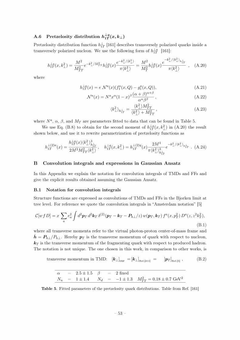
A.6 Pretzelosity distribution h⊥q1T (x, k⊥)
Pretzelosity distribution function h⊥1T [161] describes transversely polarized quarks inside atransversely polarized nucleon. We use the following form of h⊥a1T [161]:
h⊥a1T (x, k2⊥) =
M2
M2TT
e−k2⊥/M
2TT h⊥a1T (x)
e−k2⊥/〈k
2⊥〉
π〈k2⊥〉
=M2
M2T
h⊥a1T (x)e−k2⊥/〈k
2⊥〉h⊥
1T
π〈k2⊥〉
, (A.20)
where
h⊥a1T (x) = e N a(x)(fa1 (x,Q)− ga1(x,Q)), (A.21)
N a(x) = Naxα(1− x)β(α+ β)α+β
ααββ, (A.22)
〈k2⊥〉h⊥1T =
〈k2⊥〉M2
TT
〈k2⊥〉+M2
TT
, (A.23)
where Na, α, β, and MT are parameters fitted to data that can be found in Table 5.We use Eq. (B.8) to obtain for the second moment of h⊥a1T (x, k2
⊥) in (A.20) the resultshown below, and use it to rewrite parametrization of pretzelosity functions as
h⊥(2)a1T (x) =
h⊥a1T (x)〈k2⊥〉3h⊥1T
2M2M2TT 〈k2
⊥〉, h⊥q1T (x, k2
⊥) = h⊥(2)q1T (x)
2M4
π〈k2⊥〉3h⊥1T
e−k2⊥/〈k
2⊥〉h⊥
1T . (A.24)
B Convolution integrals and expressions in Gaussian Ansatz
In this Appendix we explain the notation for convolution integrals of TMDs and FFs andgive the explicit results obtained assuming the Gaussian Ansatz.
B.1 Notation for convolution integrals
Structure functions are expressed as convolutions of TMDs and FFs in the Bjorken limit attree level. For reference we quote the convolution integrals in “Amsterdam notation” [5]
C[wfD] = x∑a
e2a
∫d2pT d
2kT δ(2)(pT − kT − Ph⊥/z)w(pT ,kT ) fa(x, p2
T )Da(z, z2k2T ),
(B.1)where all transverse momenta refer to the virtual photon-proton center-of-mass frame andh = Ph⊥/Ph⊥. Hereby pT is the transverse momentum of quark with respect to nucleon,kT is the transverse momentum of the fragmenting quark with respect to produced hadron.The notation is not unique. The one chosen in this work, in comparison to other works, is
transverse momentum in TMD: [k⊥]our = [k⊥]Ref.[211] = [pT ]Ref.[5] , (B.2)
α = 2.5± 1.5 β = 2 fixedNu = 1± 1.4 Nd = −1± 1.3 M2
TT = 0.18± 0.7 GeV2
Table 5. Fitted parameters of the pretzelosity quark distributions. Table from Ref. [161]
– 53 –
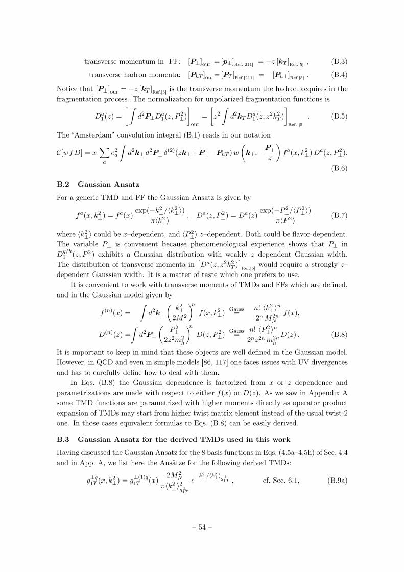
transverse momentum in FF: [P⊥]our = [p⊥]Ref.[211] = −z [kT ]Ref.[5] , (B.3)
transverse hadron momenta: [PhT ]our= [PT ]Ref.[211] = [Ph⊥]Ref.[5] . (B.4)
Notice that [P⊥]our = −z [kT ]Ref.[5] is the transverse momentum the hadron acquires in thefragmentation process. The normalization for unpolarized fragmentation functions is
Da1(z) =
[ ∫d2P⊥D
a1(z, P 2
⊥)
]our
=
[z2
∫d2kTD
a1(z, z2k2
T )
]Ref. [5]
. (B.5)
The “Amsterdam” convolution integral (B.1) reads in our notation
C[wfD] = x∑a
e2a
∫d2k⊥ d
2P⊥ δ(2)(zk⊥+P⊥−PhT )w
(k⊥,−
P⊥z
)fa(x, k2
⊥)Da(z, P 2⊥).
(B.6)
B.2 Gaussian Ansatz
For a generic TMD and FF the Gaussian Ansatz is given by
fa(x, k2⊥) = fa(x)
exp(−k2⊥/〈k2
⊥〉)π〈k2⊥〉
, Da(z, P 2⊥) = Da(z)
exp(−P 2⊥/〈P 2
⊥〉)π〈P 2
⊥〉(B.7)
where 〈k2⊥〉 could be x–dependent, and 〈P 2
⊥〉 z–dependent. Both could be flavor-dependent.The variable P⊥ is convenient because phenomenological experience shows that P⊥ inDq/h1 (z, P 2
⊥) exhibits a Gaussian distribution with weakly z–dependent Gaussian width.The distribution of transverse momenta in
[Da(z, z2k2
T )]Ref.[5]
would require a strongly z–dependent Gaussian width. It is a matter of taste which one prefers to use.
It is convenient to work with transverse moments of TMDs and FFs which are defined,and in the Gaussian model given by
f (n)(x) =
∫d2k⊥
(k2⊥
2M2
)nf(x, k2
⊥)Gauss
=n! 〈k2
⊥〉n
2nM2nN
f(x),
D(n)(z) =
∫d2P⊥
(P 2⊥
2z2m2h
)nD(z, P 2
⊥)Gauss
=n! 〈P 2
⊥〉n
2nz2nm2nh
D(z) . (B.8)
It is important to keep in mind that these objects are well-defined in the Gaussian model.However, in QCD and even in simple models [86, 117] one faces issues with UV divergencesand has to carefully define how to deal with them.
In Eqs. (B.8) the Gaussian dependence is factorized from x or z dependence andparametrizations are made with respect to either f(x) or D(z). As we saw in Appendix Asome TMD functions are parametrized with higher moments directly as operator productexpansion of TMDs may start from higher twist matrix element instead of the usual twist-2one. In those cases equivalent formulas to Eqs. (B.8) can be easily derived.
B.3 Gaussian Ansatz for the derived TMDs used in this work
Having discussed the Gaussian Ansatz for the 8 basis functions in Eqs. (4.5a–4.5h) of Sec. 4.4and in App. A, we list here the Ansätze for the following derived TMDs:
g⊥q1T (x, k2⊥) = g
⊥(1)q1T (x)
2M2N
π〈k2⊥〉2g⊥1T
e−k2⊥/〈k
2⊥〉g⊥
1T , cf. Sec. 6.1, (B.9a)
– 54 –
h⊥a1L (x, k2⊥) = h
⊥(1)a1L (x)
2M2N
π〈k2⊥〉2h⊥1L
e−k2⊥/〈k
2⊥〉
2
h⊥1L cf. Sec. 6.2, (B.9b)
gqT (x, k2⊥) = gqT (x)
1
π〈k2⊥〉gT
e−k2⊥/〈k
2⊥〉gT , cf. Sec. 7.2, (B.9c)
g⊥qT (x, k2⊥) = g
⊥(2)qT (x)
2M4
π〈k2⊥〉3g⊥T
e−k2⊥/〈k
2⊥〉g⊥
T , cf. Sec. 7.3, (B.9d)
g⊥qL (x, k2⊥) = g
⊥(1)qL (x)
2M2N
π〈k2⊥〉2g⊥L
e−k2⊥/〈k
2⊥〉g⊥
L , cf. Sec. 7.4, (B.9e)
hqL(x, k2⊥) = hqL(x)
1
π〈k2⊥〉hL
e−k2⊥/〈k
2⊥〉hL , cf. Sec. 7.5, (B.9f)
h⊥qT (x, k2⊥) = h
⊥(1)qT (x)
2M2
π〈k2⊥〉2h⊥T
e−k2⊥/〈k
2⊥〉h⊥
T , cf. Sec. 7.6, (B.9g)
hqT (x, k2⊥) = h
(1)qT (x)
2M2
π〈k2⊥〉2hT
e−k2⊥/〈k
2⊥〉hT , cf. Sec. 7.6, (B.9h)
f⊥qT (x, k2⊥) = f
⊥(2)qT (x)
2M4
π〈k2⊥〉3f⊥T
e−k2⊥/〈k
2⊥〉f⊥
T , cf. Sec. 7.7, (B.9i)
f⊥q(x, k2⊥) = f⊥(1)q(x)
2M2
π〈k2⊥〉2f⊥
e−k2⊥/〈k
2⊥〉f⊥ , cf. Sec. 7.8, (B.9j)
B.4 Comment on TMDs subject to the sum rules (2.14)
In this section we comment on the twist-3 TMDs f qT (x, k⊥), hq(x, k⊥), eqL(x, k⊥), which areT-odd, appear in the decompositions of the correlator with no explicit kj⊥–prefactors, andwould have collinear PDF counterparts. But T-odd PDFs are forbidden by time-reversaland parity invariance of strong interactions, which dictate the sum rules (2.14), see Sec. 3.8.Such TMDs could be described by functions with a node in k⊥10 such that they can integrateto zero in Eq. (2.14). A single Gaussian has no node and is not adequate for that. However,one could work with a superposition of Gaussians with different widths,
x f qT (x, k⊥) = − f⊥(1)q1T (x)
n∑i=1
aiexp(−k2
⊥/〈k2⊥〉i)
π〈k2⊥〉i
, (B.10)
n∑i=1
ai = 0 , 〈k2⊥〉i 6= 〈k2
⊥〉j ∀ i 6= j, 1 ≤ i, j ≤ n, n ≥ 2.
Notice that in (B.10) we cannot write “f qT (x)” which would be zero according to (2.14) andwe explore here the WW-type approximation (3.4g). The minimal choice would be n = 2
with a1 = −a2 = 1 and 〈k2⊥〉1 = 〈k2
⊥〉f⊥1T to make use of the theoretical guidance providedby the WW-type approximation (3.4g). The second Gaussian width 〈k2
⊥〉2 could be chosenvery large 〈k2
⊥〉2 � 〈k2⊥〉f⊥1 to model the Gaussian description of f qT (x, k⊥) similar to that
10The possibility of TMDs with nodes is not unrealistic. For instance in the covariant parton model thehelicity TMDs exhibit nodes for the u– and d–flavor [97]. We will have to revise our description of gq1(x, k⊥)
in Eq. (4.5c) and App. A.2 to something of the type (B.10), if that prediction is confirmed experimentally.
– 55 –
of f⊥(1)q1T (x, k2
⊥) at intermediate k⊥. A very large parameter 〈k2⊥〉2 could be thought of as
a relict which enters in the sum rule (2.14) where the k⊥–integration formally extends upto infinity where the TMD description does not apply. The theoretical understanding ofhigher–twist TMDs is too limited at the present stage, but in principle this could be apragmatic way of modeling the TMD f qT (x, k⊥) and analogously hq(x, k⊥), eqL(x, k⊥).
B.5 Convolution integrals in Gaussian Ansatz
Solving the convolution integrals relevant for SIDIS in the Gaussian Ansatz yields
C[ ω{0} f D] = u G(PhT ) (B.11a)
C[ω{1}A f D] = u G(PhT )
(zPhTmh
)〈P 2⊥〉
z2λ(B.11b)
C[ω{1}B f D] = −u G(PhT )
(zPhTMN
)〈k2⊥〉λ
(B.11c)
C[ω{2}A f D] = u G(PhT )〈k2⊥〉〈P 2
⊥〉λMNmh
(−1 +
2P 2hT
λ
)(B.11d)
C[ω{2}B f D] = u G(PhT )〈k2⊥〉〈P 2
⊥〉λMNmh
(1−
P 2hT
λ
)(B.11e)
C[ω{2}AB f D] = u G(PhT )
(zPhTMN
)(zPhTMh
)〈k2⊥〉λ
〈P 2⊥〉
z2λ(B.11f)
C[ω{2}C f D] =u
2G(PhT )
(zPhTMN
)(zPhTMN
)〈k2⊥〉λ
〈k2⊥〉λ
(B.11g)
C[ω{3} f D] =u
2G(PhT )
(zPhTMN
)(zPhTMN
)(zPhTmh
)〈k2⊥〉λ
〈k2⊥〉λ
〈P 2⊥〉
z2λ(B.11h)
with the ω{n}i as defined in Eq. (2.20), and we introduced the abbreviations
u = x∑a
e2af
a(x)Da(z) , G(PhT ) =exp(−P 2
hT /λ)
πλ, λ = z2〈k2
⊥〉+ 〈P 2⊥〉 , (B.12)
with the normalization∫d2PhT G(PhT ) = 1. It is important to keep in mind that strictly
speaking G(PhT ) = G(PhT , x, z) also depends on x and z. The “non-compact” notation inEqs. (B.11) was chosen to display the pattern. The masses MN or mh in the denominatorsof the PhT indicate the “origins” of the contributions: due to intrinsic k⊥ from target, dueto transverse momenta P⊥ acquired during fragmentation, or both. The weight ω{2}B is theonly which enters cross sections and does not have a homogeneous scaling in PhT .
For practical application it is convenient to absorb as many (Gaussian model) pa-rameters as possible into expressions that can be more easily fitted to data. One way toachieve this is to make use of the transverse moments (B.8). We introduce the followingabbreviations
u{1}A = x
∑a
e2af
a(x)D(1)a(z) , u{1}B = x
∑a
e2af
(1)a(x)Da(z) , (B.13)
u{2}AB = x
∑a
e2af
(1)a(x)D(1)a(z) , u{2}C = x
∑a
e2af
(2)a(x)Da(z) , (B.14)
– 56 –
u{3}C = x
∑a
e2af
(2)a(x)D(1)a(z) . (B.15)
In this notation the results in Eqs. (B.11) read
C[ω{1}A f D] = u(1)A G(PhT )
(zPhTmh
)2m2
h
λ(B.16a)
C[ω{1}B f D] = −u(1)B G(PhT )
(zPhTMN
)2M2
N
λ(B.16b)
C[ω{2}B f D] = u(2)B G(PhT )
4z2mhMN
λ
(1−
P 2hT
λ
)(B.16c)
C[ω{2}AB f D] = u(2)AB G(PhT )
(zPhTMN
)(zPhTMh
)2M2
N
λ
2m2h
λ(B.16d)
C[ω{2}C f D] =u
(2)C
2G(PhT )
(zPhTMN
)(zPhTMN
)2M2
N
λ
2M2N
λ(B.16e)
C[ω{3} f D] =u(3)
2G(PhT )
(zPhTMN
)(zPhTMN
)(zPhTmh
)2M2
N
λ
2M2N
λ
2m2h
λ(B.16f)
In this notation the results in Eqs. (B.11) read
C[ω{n}i f D] = u(n)i G(PhT ) ×
[δn2 δiB a
(2)B + b
(n)i
(zPhTλ
)n ](B.17)
with
b(0) = 1 , (B.18)
b(1)A = 2mh , b
(1)B = 2MN , (B.19)
a(2)B = 4MNmhλ
−1 z2 , b(2)AB = − b(2)
B = 4MNmh , b(2)C = M2
N , (B.20)
b(3) = 2M2Nmh . (B.21)
Finally, integrating out transverse hadron momenta yields∫d2PhT C[ω
{n}i f D] = u
(n)i c
(n)i
(z
λ1/2
)n(B.22)
with
c(0) = 1 , (B.23)
c(1)A =
√πmh , c
(1)B =
√πMN , (B.24)
c(2)AB = 4MNmh , c
(2)C = M2
N , c(2)B = 0 , (B.25)
c(3) = 32
√πM2
Nmh . (B.26)
C Mathematica package
A package available to a wide physics community is needed for several reasons. First ofall it is intended to facilitate visualization, reproduction, and verification of our results
– 57 –
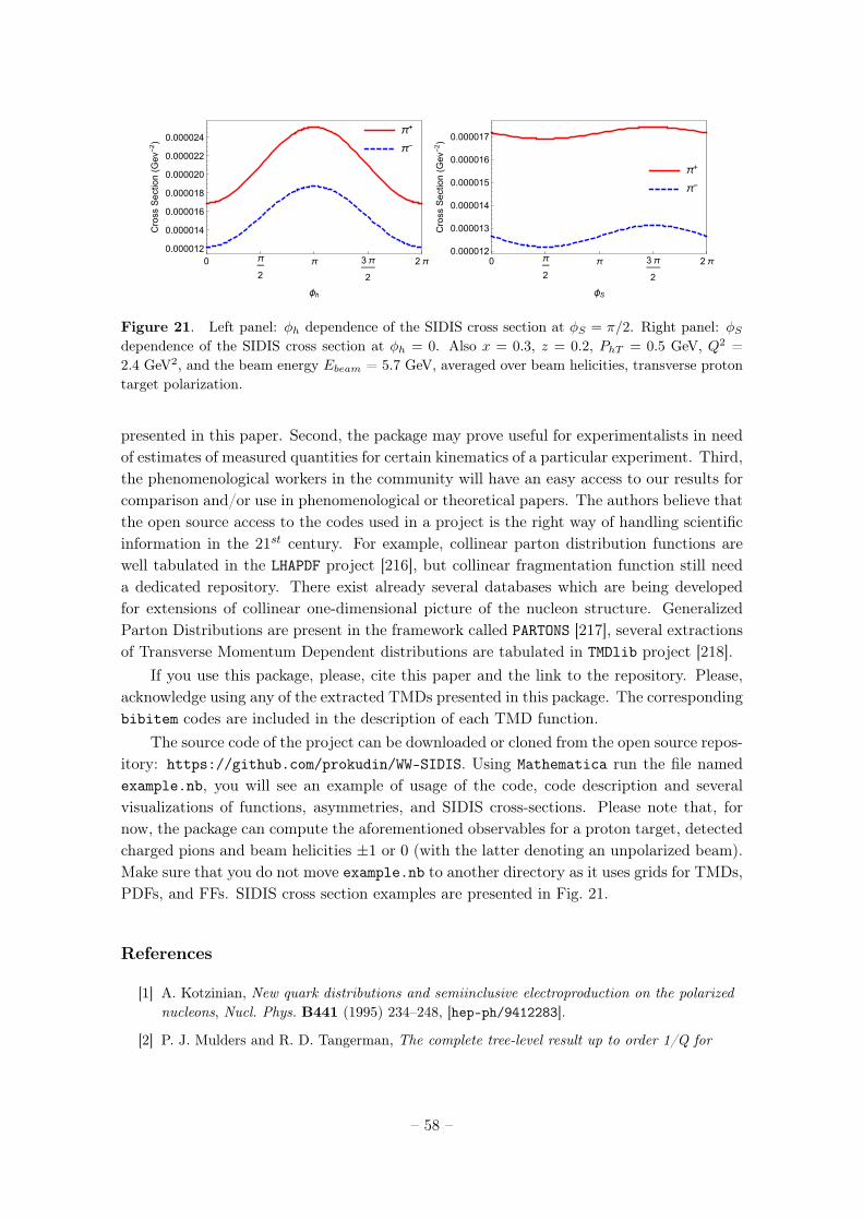
π+
π-
0 π
2
π 3π
2
2π0.000012
0.000014
0.000016
0.000018
0.000020
0.000022
0.000024
ϕh
CrossSection(Gev
-2)
π+
π-
0 π
2
π 3π
2
2π0.000012
0.000013
0.000014
0.000015
0.000016
0.000017
ϕS
CrossSection(Gev
-2)
Figure 21. Left panel: φh dependence of the SIDIS cross section at φS = π/2. Right panel: φSdependence of the SIDIS cross section at φh = 0. Also x = 0.3, z = 0.2, PhT = 0.5 GeV, Q2 =2.4 GeV2, and the beam energy Ebeam = 5.7 GeV, averaged over beam helicities, transverse protontarget polarization.
presented in this paper. Second, the package may prove useful for experimentalists in needof estimates of measured quantities for certain kinematics of a particular experiment. Third,the phenomenological workers in the community will have an easy access to our results forcomparison and/or use in phenomenological or theoretical papers. The authors believe thatthe open source access to the codes used in a project is the right way of handling scientificinformation in the 21st century. For example, collinear parton distribution functions arewell tabulated in the LHAPDF project [216], but collinear fragmentation function still needa dedicated repository. There exist already several databases which are being developedfor extensions of collinear one-dimensional picture of the nucleon structure. GeneralizedParton Distributions are present in the framework called PARTONS [217], several extractionsof Transverse Momentum Dependent distributions are tabulated in TMDlib project [218].
If you use this package, please, cite this paper and the link to the repository. Please,acknowledge using any of the extracted TMDs presented in this package. The correspondingbibitem codes are included in the description of each TMD function.
The source code of the project can be downloaded or cloned from the open source repos-itory: https://github.com/prokudin/WW-SIDIS. Using Mathematica run the file namedexample.nb, you will see an example of usage of the code, code description and severalvisualizations of functions, asymmetries, and SIDIS cross-sections. Please note that, fornow, the package can compute the aforementioned observables for a proton target, detectedcharged pions and beam helicities ±1 or 0 (with the latter denoting an unpolarized beam).Make sure that you do not move example.nb to another directory as it uses grids for TMDs,PDFs, and FFs. SIDIS cross section examples are presented in Fig. 21.
References
[1] A. Kotzinian, New quark distributions and semiinclusive electroproduction on the polarizednucleons, Nucl. Phys. B441 (1995) 234–248, [hep-ph/9412283].
[2] P. J. Mulders and R. D. Tangerman, The complete tree-level result up to order 1/Q for
– 58 –
polarized deep-inelastic leptoproduction, Nucl. Phys. B461 (1996) 197–237,[hep-ph/9510301].
[3] D. Boer and P. J. Mulders, Time-reversal odd distribution functions in leptoproduction,Phys. Rev. D57 (1998) 5780–5786, [hep-ph/9711485].
[4] K. Goeke, A. Metz and M. Schlegel, Parameterization of the quark–quark correlator of aspin-1/2 hadron, Phys. Lett. B618 (2005) 90–96, [hep-ph/0504130].
[5] A. Bacchetta, M. Diehl, K. Goeke, A. Metz, P. J. Mulders and M. Schlegel, Semi-inclusivedeep inelastic scattering at small transverse momentum, JHEP 02 (2007) 093,[hep-ph/0611265].
[6] F. Stock et al., The FILTEX / HERMES polarized hydrogen atomic beam source, Nucl.Instrum. Meth. A343 (1994) 334–342.
[7] HERMES collaboration, A. Airapetian et al., The HERMES polarized hydrogen anddeuterium gas target in the HERA electron storage ring, Nucl. Instrum. Meth. A540 (2005)68–101, [physics/0408137].
[8] D. G. Crabb and W. Meyer, Solid polarized targets for nuclear and particle physicsexperiments, Ann. Rev. Nucl. Part. Sci. 47 (1997) 67–109.
[9] S. Goertz, W. Meyer and G. Reicherz, Polarized H, D and 3He targets for particle physicsexperiments, Prog. Part. Nucl. Phys. 49 (2002) 403–489.
[10] S. Arnold, A. Metz and M. Schlegel, Dilepton production from polarized hadron hadroncollisions, Phys. Rev. D79 (2009) 034005, [0809.2262].
[11] A. Metz and A. Vossen, Parton fragmentation functions, Prog. Part. Nucl. Phys. 91 (2016)136–202, [1607.02521].
[12] G. A. Miller, Densities, parton distributions, and measuring the nonspherical shape of thenucleon, Phys. Rev. C76 (2007) 065209, [0708.2297].
[13] M. Burkardt, Spin-orbit correlations and single-spin asymmetries, in Workshop on ExclusiveReactions at High Momentum Transfer Newport News, Virginia, May 21-24, 2007, 2007.0709.2966.
[14] M. Burkardt, The g2 Structure Function, AIP Conf.Proc. 1155 (2009) 26–34, [0905.4079].
[15] A. Bacchetta, M. Boglione, A. Henneman and P. J. Mulders, Bounds on TransverseMomentum Dependent Distribution and Fragmentation Functions, Phys. Rev. Lett. 85(2000) 712–715, [hep-ph/9912490].
[16] S. Wandzura and F. Wilczek, Sum rules for spin-dependent electroproduction: Test ofrelativistic constituent quarks, Phys. Lett. B72 (1977) 195.
[17] R. Jaffe and X. Ji, Chiral-odd parton distributions and Drell–Yan processes, Nucl. Phys.B375 (1992) 527–560.
[18] R. L. Jaffe, g2-The Nucleon’s Other Spin-Dependent Structure Function, Comments Nucl.Part. Phys. 19 (1990) 239–257.
[19] J. Balla, M. V. Polyakov and C. Weiss, Nucleon matrix elements of higher-twist operatorsfrom the instanton vacuum, Nucl. Phys. B510 (1998) 327–364, [hep-ph/9707515].
[20] B. Dressler and M. V. Polyakov, Twist-three contribution to hL in the instanton vacuum,Phys. Rev. D61 (2000) 097501, [hep-ph/9912376].
– 59 –
[21] M. Göckeler, R. Horsley, W. Kürzinger, H. Oelrich, D. Pleiter et al., Lattice calculation ofthe nucleon’s spin-dependent structure function g2 reexamined, Phys. Rev. D63 (2001)074506, [hep-lat/0011091].
[22] M. Göckeler, R. Horsley, D. Pleiter, P. E. Rakow, A. Schäfer et al., Investigation of thesecond moment of the nucleon’s g1 and g2 structure functions in two-flavor lattice QCD,Phys. Rev. D72 (2005) 054507, [hep-lat/0506017].
[23] E143 collaboration, K. Abe et al., Measurements of the proton and deuteron spin structurefunctions g1 and g2, Phys. Rev. D58 (1998) 112003, [hep-ph/9802357].
[24] E155 collaboration, P. L. Anthony et al., Precision measurement of the proton anddeuteron spin structure functions g2 and asymmetries A2, Phys. Lett. B553 (2003) 18–24,[hep-ex/0204028].
[25] HERMES collaboration, A. Airapetian et al., Measurement of the virtual-photonasymmetry A2 and the spin-structure function g2 of the proton, Eur. Phys. J. C72 (2012)1921, [1112.5584].
[26] A. M. Kotzinian and P. J. Mulders, Longitudinal quark polarization in transversely polarizednucleons, Phys. Rev. D54 (1996) 1229–1232, [hep-ph/9511420].
[27] A. M. Kotzinian and P. J. Mulders, Probing transverse quark polarization via azimuthalasymmetries in leptoproduction, Phys. Lett. B406 (1997) 373–380, [hep-ph/9701330].
[28] A. Kotzinian, B. Parsamyan and A. Prokudin, Predictions for double spin asymmetry ALTin semiinclusive DIS, Phys. Rev. D73 (2006) 114017, [hep-ph/0603194].
[29] H. Avakian et al., Are there approximate relations among transverse momentum dependentdistribution functions?, Phys. Rev. D77 (2008) 014023, [0709.3253].
[30] A. Metz, P. Schweitzer and T. Teckentrup, Lorentz invariance relations between partondistributions and the Wandzura–Wilczek approximation, Phys. Lett. B680 (2009) 141–147,[0810.5212].
[31] T. Teckentrup, A. Metz and P. Schweitzer, Lorentz invariance relations andWandzura–Wilczek approximation, Mod. Phys. Lett. A24 (2009) 2950–2959, [0910.2567].
[32] R. Tangerman and P. Mulders, Polarized twist-three distributions gT and hL and the role ofintrinsic transverse momentum, hep-ph/9408305.
[33] H. Avakian, H. Matevosyan, B. Pasquini and P. Schweitzer, Studying the informationcontent of TMDs using Monte Carlo generators, J. Phys. G42 (2015) 034015.
[34] A. Metz and M. Schlegel, Twist-3 single-spin asymmetries in semi-inclusive deep-inelasticscattering, Eur. Phys. J. A22 (2004) 489–494, [hep-ph/0403182].
[35] L. P. Gamberg, D. S. Hwang, A. Metz and M. Schlegel, Light-cone divergence in twist-3correlation functions, Phys. Lett. B639 (2006) 508–512, [hep-ph/0604022].
[36] W. R. Inc., “Mathematica, Version 11.3.”
[37] J. C. Collins, Leading-twist single-transverse-spin asymmetries: Drell–Yan anddeep-inelastic scattering, Phys. Lett. B536 (2002) 43–48, [hep-ph/0204004].
[38] J. P. Ralston and D. E. Soper, Production of Dimuons from High-Energy Polarized ProtonProton Collisions, Nucl. Phys. B152 (1979) 109.
[39] J. C. Collins and D. E. Soper, Back-To-Back Jets in QCD, Nucl. Phys. B193 (1981) 381.
– 60 –
[40] X. Ji, J.-P. Ma and F. Yuan, QCD factorization for semi-inclusive deep-inelastic scatteringat low transverse momentum, Phys. Rev. D71 (2005) 034005, [hep-ph/0404183].
[41] X. Ji, J.-P. Ma and F. Yuan, QCD factorization for spin-dependent cross sections in DISand Drell-Yan processes at low transverse momentum, Phys. Lett. B597 (2004) 299–308,[hep-ph/0405085].
[42] J. Collins, Foundations of perturbative QCD, Camb. Monogr. Part. Phys. Nucl. Phys.Cosmol. 32 (2011) 1–624.
[43] M. G. Echevarría, A. Idilbi and I. Scimemi, Soft and collinear factorization and transversemomentum dependent parton distribution functions, Phys. Lett. B726 (2013) 795–801,[1211.1947].
[44] S. M. Aybat and T. C. Rogers, TMD Parton Distribution and Fragmentation Functionswith QCD Evolution, Phys. Rev. D83 (2011) 114042, [1101.5057].
[45] S. M. Aybat, J. C. Collins, J.-W. Qiu and T. C. Rogers, The QCD Evolution of the SiversFunction, Phys. Rev. D85 (2012) 034043, [1110.6428].
[46] M. G. Echevarria, A. Idilbi, Z.-B. Kang and I. Vitev, QCD Evolution of the SiversAsymmetry, Phys. Rev. D89 (2014) 074013, [1401.5078].
[47] J. Collins and T. Rogers, Understanding the large-distance behavior oftransverse-momentum-dependent parton densities and the Collins-Soper evolution kernel,Phys. Rev. D91 (2015) 074020, [1412.3820].
[48] J. P. Ma and G. P. Zhang, QCD corrections of all structure functions in transversemomentum dependent factorization for Drell–Yan processes, JHEP 02 (2014) 100,[1308.2044].
[49] S. M. Aybat, A. Prokudin and T. C. Rogers, Calculation of TMD Evolution for TransverseSingle Spin Asymmetry Measurements, Phys. Rev. Lett. 108 (2012) 242003, [1112.4423].
[50] Z.-B. Kang, A. Prokudin, P. Sun and F. Yuan, Extraction of quark transversity distributionand Collins fragmentation functions with QCD evolution, Phys. Rev. D93 (2016) 014009,[1505.05589].
[51] D. Gutiérrez-Reyes, I. Scimemi and A. A. Vladimirov, Twist-2 matching of transversemomentum dependent distributions, Phys. Lett. B769 (2017) 84–89, [1702.06558].
[52] D. Gutierrez-Reyes, I. Scimemi, W. J. Waalewijn and L. Zoppi,Transverse-Momentum-Dependent Distributions with Jets, Phys. Rev. Lett. 121 (2018)162001, [1807.07573].
[53] I. Scimemi and A. Vladimirov, Matching of transverse momentum dependent distributionsat twist-3, Eur. Phys. J. C78 (2018) 802, [1804.08148].
[54] A. P. Chen and J. P. Ma, Light-cone singularities and transverse-momentum-dependentfactorization at twist-3, Phys. Lett. B768 (2017) 380–386, [1610.08634].
[55] A. V. Efremov and P. Schweitzer, The chirally-odd twist-3 distribution ea(x), JHEP 08(2003) 006, [hep-ph/0212044].
[56] R. L. Jaffe, Spin, twist and hadron structure in deep inelastic processes, in The spinstructure of the nucleon. Proceedings, International School of Nucleon Structure, 1stCourse, Erice, Italy, August 3-10, 1995, pp. 42–129, 1996. hep-ph/9602236.
– 61 –
[57] K. Kanazawa, Y. Koike, A. Metz, D. Pitonyak and M. Schlegel, Operator constraints fortwist-3 functions and Lorentz invariance properties of twist-3 observables, Phys. Rev. D93(2016) 054024, [1512.07233].
[58] E. V. Shuryak, The role of instantons in quantum chromodynamics: (I). Physical vacuum,Nucl. Phys. B203 (1982) 93.
[59] D. Diakonov and V. Y. Petrov, Instanton-based vacuum from Feynman variationalprinciple, Nucl. Phys. B245 (1984) 259.
[60] D. Diakonov, M. V. Polyakov and C. Weiss, Hadronic matrix elements of gluon operators inthe instanton vacuum, Nucl. Phys. B461 (1996) 539–580, [hep-ph/9510232].
[61] Spin Muon collaboration, D. Adams et al., Spin asymmetry in muon-proton deep inelasticscattering on a transversely polarized target, Phys. Lett. B336 (1994) 125–130,[hep-ex/9408001].
[62] A. Accardi, A. Bacchetta, W. Melnitchouk and M. Schlegel, What can break theWandzura–Wilczek relation?, JHEP 11 (2009) 093, [0907.2942].
[63] M. Glück, E. Reya and A. Vogt, Dynamical parton distributions revisited, Eur. Phys. J. C5(1998) 461–470, [hep-ph/9806404].
[64] A. V. Efremov, K. Goeke and P. Schweitzer, Collins effect in semiinclusive deeply inelasticscattering and in electron-positron-annihilation, Phys. Rev. D73 (2006) 094025,[hep-ph/0603054].
[65] M. Anselmino et al., Transversity and Collins functions from SIDIS and e+e− data, Phys.Rev. D75 (2007) 054032, [hep-ph/0701006].
[66] M. Anselmino et al., Update on transversity and Collins functions from SIDIS and e+e−
data, Nucl. Phys. Proc. Suppl. 191 (2009) 98–107, [0812.4366].
[67] Y. Koike, K. Tanaka and S. Yoshida, Drell–Yan double-spin asymmetry ALT in polarized ppcollisions: Wandzura–Wilczek contribution, Phys. Lett. B668 (2008) 286–292, [0805.2289].
[68] P. Hägler, B. U. Musch, J. W. Negele and A. Schäfer, Intrinsic quark transverse momentumin the nucleon from lattice QCD, Europhys. Lett. 88 (2009) 61001, [0908.1283].
[69] B. U. Musch, P. Hägler, J. W. Negele and A. Schäfer, Exploring quark transversemomentum distributions with lattice QCD, Phys. Rev. D83 (2011) 094507, [1011.1213].
[70] B. Yoon, M. Engelhardt, R. Gupta, T. Bhattacharya, J. R. Green, B. U. Musch et al.,Nucleon transverse-momentum-dependent parton distributions in lattice QCD:Renormalization patterns and discretization effects, Phys. Rev. D96 (2017) 094508,[1706.03406].
[71] M. Engelhardt, P. Hägler, B. Musch, J. Negele and A. Schäfer, Lattice QCD study of theBoer-Mulders effect in a pion, Phys. Rev. D93 (2016) 054501, [1506.07826].
[72] X. Ji, P. Sun, X. Xiong and F. Yuan, Soft factor subtraction and transverse momentumdependent parton distributions on the lattice, Phys. Rev. D91 (2015) 074009, [1405.7640].
[73] B. U. Musch, P. Hägler, M. Engelhardt, J. W. Negele and A. Schäfer, Sivers andBoer-Mulders observables from lattice QCD, Phys. Rev. D85 (2012) 094510, [1111.4249].
[74] C. Alexandrou, S. Bacchio, K. Cichy, M. Constantinou, K. Hadjiyiannakou, K. Jansenet al., Computation of parton distributions from the quasi-PDF approach at the physicalpoint, EPJ Web Conf. 175 (2018) 14008, [1710.06408].
– 62 –
[75] T. Ishikawa, Y.-Q. Ma, J.-W. Qiu and S. Yoshida, Renormalizability of quasipartondistribution functions, Phys. Rev. D96 (2017) 094019, [1707.03107].
[76] X. Ji, J.-H. Zhang and Y. Zhao, Renormalization in Large Momentum Effective Theory ofParton Physics, Phys. Rev. Lett. 120 (2018) 112001, [1706.08962].
[77] J. Green, K. Jansen and F. Steffens, Nonperturbative Renormalization of Nonlocal QuarkBilinears for Parton Quasidistribution Functions on the Lattice Using an Auxiliary Field,Phys. Rev. Lett. 121 (2018) 022004, [1707.07152].
[78] J.-H. Zhang, J.-W. Chen, X. Ji, L. Jin and H.-W. Lin, Pion distribution amplitude fromlattice QCD, Phys. Rev. D95 (2017) 094514, [1702.00008].
[79] LHPC and SESAM collaboration, LHPC, P. Hägler, J. W. Negele, D. B. Renner,W. Schroers, T. Lippert et al., Transverse structure of nucleon parton distributions fromlattice QCD, Phys. Rev. Lett. 93 (2004) 112001, [hep-lat/0312014].
[80] LHPC collaboration, P. Hägler, W. Schroers, J. Bratt, J. W. Negele, A. V. Pochinsky,R. G. Edwards et al., Nucleon generalized parton distributions from full lattice QCD, Phys.Rev. D77 (2008) 094502, [0705.4295].
[81] QCDSF and UKQCD collaboration, M. Göckeler, P. Hägler, R. Horsley, D. Pleiter,P. E. L. Rakow, A. Schäfer et al., Quark helicity flip generalized parton distributions fromtwo-flavor lattice QCD, Phys. Lett. B627 (2005) 113–123, [hep-lat/0507001].
[82] M. Burkardt and Y. Koike, Violation of sum rules for twist-3 parton distributions in QCD,Nucl. Phys. B632 (2002) 311–329, [hep-ph/0111343].
[83] S. D. Bass, Fixed poles, polarized glue and nucleon spin structure, Acta Phys. Polon. B34(2003) 5893–5926, [hep-ph/0311174].
[84] M. Stratmann, Bag model predictions for polarized structure functions and theirQ2-evolutions, Z. Phys. C60 (1993) 763–772.
[85] A. Signal, Calculations of higher twist distribution functions in the MIT bag model, Nucl.Phys. B497 (1997) 415–434, [hep-ph/9610480].
[86] H. Avakian, A. Efremov, P. Schweitzer and F. Yuan, The transverse momentum dependentdistribution functions in the bag model, Phys. Rev. D81 (2010) 074035, [1001.5467].
[87] R. Jakob, P. Mulders and J. Rodrigues, Modeling quark distribution and fragmentationfunctions, Nucl. Phys. A626 (1997) 937–965, [hep-ph/9704335].
[88] M. Wakamatsu, Polarized structure functions g2(x) in the chiral quark soliton model, Phys.Lett. B487 (2000) 118–124, [hep-ph/0006212].
[89] B. Pasquini, S. Cazzaniga and S. Boffi, Transverse momentum dependent partondistributions in a light-cone quark model, Phys. Rev. D78 (2008) 034025, [0806.2298].
[90] C. Lorcé, B. Pasquini and M. Vanderhaeghen, Unified framework for generalized andtransverse-momentum dependent parton distributions within a 3Q light-cone picture of thenucleon, JHEP 1105 (2011) 041, [1102.4704].
[91] R. Kundu and A. Metz, Higher twist and transverse momentum dependent partondistributions: A Light front Hamiltonian approach, Phys. Rev. D65 (2002) 014009,[hep-ph/0107073].
[92] M. Schlegel and A. Metz, On the validity of Lorentz invariance relations between parton
– 63 –
distributions, in Proceedings, 10th Advanced Research Workshop on High-Energy SpinPhysics, Dubna, Russia, September 16-20, 2003, pp. 169–173, 2004. hep-ph/0406289.
[93] K. Goeke, A. Metz, P. Pobylitsa and M. Polyakov, Lorentz invariance relations amongparton distributions revisited, Phys. Lett. B567 (2003) 27–30, [hep-ph/0302028].
[94] C. Lorcé, B. Pasquini and P. Schweitzer, Unpolarized transverse momentum dependentparton distribution functions beyond leading twist in quark models, JHEP 01 (2015) 103,[1411.2550].
[95] C. Lorcé, B. Pasquini and P. Schweitzer, Transverse pion structure beyond leading twist inconstituent models, Eur. Phys. J. C76 (2016) 415, [1605.00815].
[96] P. Zavada, The Structure functions and parton momenta distribution in the hadron restsystem, Phys. Rev. D55 (1997) 4290–4299, [hep-ph/9609372].
[97] A. V. Efremov, P. Schweitzer, O. V. Teryaev and P. Zavada, The relation between TMDsand PDFs in the covariant parton model approach, Phys. Rev. D83 (2011) 054025,[1012.5296].
[98] A. V. Efremov, P. Schweitzer, O. V. Teryaev and P. Zavada, Transverse momentumdependent distribution functions in a covariant parton model approach with quark orbitalmotion, Phys. Rev. D80 (2009) 014021, [0903.3490].
[99] P. Schweitzer, Chirally-odd twist-3 distribution function ea(x) in the chiral quark-solitonmodel, Phys. Rev. D67 (2003) 114010, [hep-ph/0303011].
[100] Y. Ohnishi and M. Wakamatsu, πN sigma term and chira-odd twist-3 distribution functione(x) of the nucleon in the chiral quark soliton model, Phys. Rev. D69 (2004) 114002,[hep-ph/0312044].
[101] C. Cebulla, J. Ossmann, P. Schweitzer and D. Urbano, The Twist-3 Parton DistributionFunction ea(x) in Large-Nc Chiral Theory, Acta Phys. Polon. B39 (2008) 609–640,[0710.3103].
[102] S. Meissner, A. Metz and K. Goeke, Relations between generalized and transversemomentum dependent parton distributions, Phys. Rev. D76 (2007) 034002,[hep-ph/0703176].
[103] A. Mukherjee, Twist Three Distribution e(x): Sum Rules and Equation of Motion Relations,Phys. Lett. B687 (2010) 180–183, [0912.1446].
[104] A. Harindranath and W.-M. Zhang, Examination of Wandzura–Wilczek relation forg2(x,Q2) in pQCD, Phys. Lett. B408 (1997) 347–356, [hep-ph/9706419].
[105] D. Boer, P. J. Mulders and F. Pijlman, Universality of T-odd effects in single spin andazimuthal asymmetries, Nucl. Phys. B667 (2003) 201–241, [hep-ph/0303034].
[106] X. Ji, J.-W. Qiu, W. Vogelsang and F. Yuan, Unified Picture for Single Transverse-SpinAsymmetries in Hard-Scattering Processes, Phys. Rev. Lett. 97 (2006) 082002,[hep-ph/0602239].
[107] M. Anselmino et al., The role of Cahn and Sivers effects in deep inelastic scattering, Phys.Rev. D71 (2005) 074006, [hep-ph/0501196].
[108] J. C. Collins, A. V. Efremov, K. Goeke, S. Menzel, A. Metz and P. Schweitzer, Sivers effectin semiinclusive deeply inelastic scattering, Phys. Rev. D73 (2006) 014021,[hep-ph/0509076].
– 64 –
[109] U. D’Alesio and F. Murgia, Azimuthal and single spin asymmetries in hard scatteringprocesses, Prog. Part. Nucl. Phys. 61 2008 (2008) 394–454, [0712.4328].
[110] P. Schweitzer, T. Teckentrup and A. Metz, Intrinsic transverse parton momenta in deeplyinelastic reactions, Phys. Rev. D81 (2010) 094019, [1003.2190].
[111] A. Signori, A. Bacchetta, M. Radici and G. Schnell, Investigations into the flavordependence of partonic transverse momentum, JHEP 11 (2013) 194, [1309.3507].
[112] M. Anselmino, M. Boglione, J. O. Gonzalez Hernandez, S. Melis and A. Prokudin,Unpolarised transverse momentum dependent distribution and fragmentation functions fromSIDIS multiplicities, JHEP 04 (2014) 005, [1312.6261].
[113] A. Bacchetta, D. Boer, M. Diehl and P. J. Mulders, Matches and mismatches in thedescriptions of semi-inclusive processes at low and high transverse momentum, JHEP 08(2008) 023, [0803.0227].
[114] F. Landry, R. Brock, P. M. Nadolsky and C. Yuan, Tevatron run-1 Z boson data andCollins-Soper-Sterman resummation formalism, Phys. Rev. D67 (2003) 073016,[hep-ph/0212159].
[115] A. D. Martin, W. J. Stirling, R. S. Thorne and G. Watt, Parton distributions for the LHC,Eur. Phys. J. C63 (2009) 189–285, [0901.0002].
[116] D. de Florian, R. Sassot and M. Stratmann, Global analysis of fragmentation functions forpions and kaons and their uncertainties, Phys. Rev. D75 (2007) 114010, [hep-ph/0703242].
[117] P. Schweitzer, M. Strikman and C. Weiss, Intrinsic transverse momentum and partoncorrelations from dynamical chiral symmetry breaking, JHEP 01 (2013) 163, [1210.1267].
[118] J. Collins, L. Gamberg, A. Prokudin, T. C. Rogers, N. Sato and B. Wang, Relatingtransverse-momentum-dependent and collinear factorization theorems in a generalizedformalism, Phys. Rev. D94 (2016) 034014, [1605.00671].
[119] CLAS collaboration, M. Osipenko et al., Measurement of unpolarized semi-inclusive π+
electroproduction off the proton, Phys. Rev. D80 (2009) 032004, [0809.1153].
[120] HERMES collaboration, A. Airapetian et al., Multiplicities of charged pions and kaonsfrom semi-inclusive deep-inelastic scattering by the proton and the deuteron, Phys. Rev.D87 (2013) 074029, [1212.5407].
[121] COMPASS collaboration, M. Aghasyan et al., Transverse-momentum-dependentmultiplicities of charged hadrons in muon-deuteron deep inelastic scattering, Phys. Rev.D97 (2018) 032006, [1709.07374].
[122] A. Bacchetta, F. Delcarro, C. Pisano, M. Radici and A. Signori, Extraction of partonictransverse momentum distributions from semi-inclusive deep-inelastic scattering, Drell–Yanand Z-boson production, JHEP 06 (2017) 081, [1703.10157].
[123] CLAS collaboration, H. Avakian et al., Measurement of Single- and Double-SpinAsymmetries in Deep Inelastic Pion Electroproduction with a Longitudinally PolarizedTarget, Phys. Rev. Lett. 105 (2010) 262002, [1003.4549].
[124] M. Anselmino, M. Boglione, U. D’Alesio, S. Melis, F. Murgia and A. Prokudin, SiversDistribution Functions and the Latest SIDIS Data, in 19th International Workshop onDeep-Inelastic Scattering and Related Subjects (DIS 2011) Newport News, Virginia, April11-15, 2011, 2011. 1107.4446.
– 65 –
[125] HERMES collaboration, A. Airapetian et al., Observation of the Naive-T-odd Sivers Effectin Deep-Inelastic Scattering, Phys. Rev. Lett. 103 (2009) 152002, [0906.3918].
[126] COMPASS collaboration, C. Adolph et al., II Experimental investigation of transverse spinasymmetries in µ-p SIDIS processes: Sivers asymmetries, Phys. Lett. B717 (2012) 383–389,[1205.5122].
[127] D. W. Sivers, Single-spin production asymmetries from the hard scattering of pointlikeconstituents, Phys. Rev. D41 (1990) 83.
[128] M. Anselmino, M. Boglione, U. D’Alesio, S. Melis, F. Murgia and A. Prokudin, New insighton the Sivers transverse momentum dependent distribution function, J. Phys. Conf. Ser.295 (2011) 012062, [1012.3565].
[129] M. Anselmino, M. Boglione, U. D’Alesio, A. Kotzinian, F. Murgia and A. Prokudin,Extracting the Sivers function from polarized semi-inclusive deep inelastic scattering dataand making predictions, Phys. Rev. D72 (2005) 094007, [hep-ph/0507181].
[130] M. Anselmino et al., Comparing extractions of Sivers functions, in Transversity.Proceedings, Workshop, Como, Italy, September 7-10, 2005, pp. 236–243, 2005.hep-ph/0511017.
[131] W. Vogelsang and F. Yuan, Single-transverse-spin asymmetries: From deep inelasticscattering to hadronic collisions, Phys. Rev. D72 (2005) 054028, [hep-ph/0507266].
[132] M. Anselmino, M. Boglione, U. D’Alesio, A. Kotzinian, S. Melis, F. Murgia et al., Siverseffect for pion and kaon production in semi-inclusive deep inelastic scattering, Eur. Phys. J.A39 (2009) 89–100, [0805.2677].
[133] A. Bacchetta and M. Radici, Constraining Quark Angular Momentum throughSemi-Inclusive Measurements, Phys. Rev. Lett. 107 (2011) 212001, [1107.5755].
[134] M. Anselmino, M. Boglione and S. Melis, Strategy towards the extraction of the Siversfunction with transverse momentum dependent evolution, Phys. Rev. D86 (2012) 014028,[1204.1239].
[135] A. Bacchetta and M. Radici, Partial-wave analysis of two-hadron fragmentation functions,Phys. Rev. D67 (2003) 094002, [hep-ph/0212300].
[136] A. Bacchetta and M. Radici, Two-hadron semi-inclusive production including subleadingtwist contributions, Phys. Rev. D69 (2004) 074026, [hep-ph/0311173].
[137] A. Bacchetta, A. Courtoy and M. Radici, First Glances at the Transversity PartonDistribution through Dihadron Fragmentation Functions, Phys. Rev. Lett. 107 (2011)012001, [1104.3855].
[138] A. Bacchetta, A. Courtoy and M. Radici, First extraction of valence transversities in acollinear framework, JHEP 03 (2013) 119, [1212.3568].
[139] M. Radici, A. Courtoy, A. Bacchetta and M. Guagnelli, Improved extraction of valencetransversity distributions from inclusive dihadron production, JHEP 05 (2015) 123,[1503.03495].
[140] M. Radici and A. Bacchetta, First Extraction of Transversity from a Global Analysis ofElectron-Proton and Proton-Proton Data, Phys. Rev. Lett. 120 (2018) 192001,[1802.05212].
– 66 –
[141] COMPASS collaboration, M. Aghasyan et al., First Measurement ofTransverse-Spin-Dependent Azimuthal Asymmetries in the Drell–Yan Process, Phys. Rev.Lett. 119 (2017) 112002, [1704.00488].
[142] COMPASS collaboration, B. Parsamyan, First measurement of transverse-spin-dependentazimuthal asymmetries in the Drell-Yan process, PoS DIS2017 (2018) 243, [1801.01487].
[143] J. C. Collins, Fragmentation of transversely polarized quarks probed in transversemomentum distributions, Nucl. Phys. B396 (1993) 161–182.
[144] M. Anselmino, M. Boglione, U. D’Alesio, S. Melis, F. Murgia and A. Prokudin,Simultaneous extraction of transversity and Collins functions from new SIDIS and e+e−
data, Phys. Rev. D87 (2013) 094019, [1303.3822].
[145] Z.-B. Kang, A. Prokudin, P. Sun and F. Yuan, Nucleon tensor charge from Collinsazimuthal asymmetry measurements, Phys. Rev. D91 (2015) 071501, [1410.4877].
[146] M. Anselmino, M. Boglione, U. D’Alesio, J. O. Gonzalez Hernandez, S. Melis, F. Murgiaet al., Collins functions for pions from SIDIS and new e+e− data: a first glance at theirtransverse momentum dependence, Phys. Rev. D92 (2015) 114023, [1510.05389].
[147] HERMES collaboration, A. Airapetian et al., Effects of transversity in deep-inelasticscattering by polarized protons, Phys. Lett. B693 (2010) 11–16, [1006.4221].
[148] COMPASS collaboration, C. Adolph et al., Collins and Sivers asymmetries inmuonproduction of pions and kaons off transversely polarised protons, Phys. Lett. B744(2015) 250–259, [1408.4405].
[149] V. Barone, S. Melis and A. Prokudin, The Boer-Mulders effect in unpolarized SIDIS: AnAnalysis of the COMPASS and HERMES data on the cos2phi asymmetry, Phys. Rev. D81(2010) 114026, [0912.5194].
[150] HERMES collaboration, A. Airapetian et al., Azimuthal distributions of charged hadrons,pions, and kaons produced in deep-inelastic scattering off unpolarized protons anddeuterons, Phys. Rev. D87 (2013) 012010, [1204.4161].
[151] COMPASS collaboration, C. Adolph et al., Measurement of azimuthal hadron asymmetriesin semi-inclusive deep inelastic scattering off unpolarised nucleons, Nucl. Phys. B886(2014) 1046–1077, [1401.6284].
[152] R. N. Cahn, Azimuthal dependence in leptoproduction: A simple parton model calculation,Phys. Lett. B78 (1978) 269.
[153] X. Cao, Parton distributions and cos 2φh asymmetry induced by anomalous photon-quarkcoupling, Phys. Rev. D97 (2018) 114010, [1802.02417].
[154] V. Barone, S. Melis and A. Prokudin, Azimuthal asymmetries in unpolarized Drell–Yanprocesses and the Boer–Mulders distributions of antiquarks, Phys. Rev. D82 (2010) 114025,[1009.3423].
[155] V. Barone, M. Boglione, J. O. Gonzalez Hernandez and S. Melis, Phenomenological analysisof azimuthal asymmetries in unpolarized semi-inclusive deep inelastic scattering, Phys. Rev.D91 (2015) 074019, [1502.04214].
[156] H. Avakian, A. V. Efremov, P. Schweitzer and F. Yuan, Transverse momentum dependentdistribution function h⊥1T and the single spin asymmetry Asin(3φ−φS)
UT , Phys. Rev. D78(2008) 114024, [0805.3355].
– 67 –
[157] J. She, J. Zhu and B.-Q. Ma, h⊥1T and quark orbital angular momentum, Phys. Rev. D79(2009) 054008, [0902.3718].
[158] C. Lorce and B. Pasquini, The pretzelosity TMD and quark orbital angular momentum,Phys. Lett. B710 (2012) 486–488, [1111.6069].
[159] COMPASS collaboration, B. Parsamyan, Transverse spin asymmetries at COMPASS:beyond Collins and Sivers effects, PoS DIS2013 (2013) 231, [1307.0183].
[160] HERMES collaboration, G. Schnell, The Sivers and other semi-inclusive single-spinasymmetries at HERMES, PoS DIS2010 (2010) 247.
[161] C. Lefky and A. Prokudin, Extraction of the distribution function h⊥1T from experimentaldata, Phys. Rev. D91 (2015) 034010, [1411.0580].
[162] A. Kotzinian, SIDIS Asymmetries in Quark-Diquark Model, in Transversity 2008: 2ndInternational Workshop on Transverse Polarization Phenomena in Hard Processes Ferrara,Italy, May 28-31, 2008, 2008. 0806.3804.
[163] S. Boffi, A. V. Efremov, B. Pasquini and P. Schweitzer, Azimuthal spin asymmetries inlight-cone constituent quark models, Phys. Rev. D79 (2009) 094012, [0903.1271].
[164] NNPDF collaboration, R. D. Ball et al., Parton distributions for the LHC Run II, JHEP04 (2015) 040, [1410.8849].
[165] Jefferson Lab Hall A collaboration, J. Huang et al., Beam-Target Double SpinAsymmetry ALT in Charged Pion Production from Deep Inelastic Scattering on aTransversely Polarized 3He Target at 1.4 < Q2 < 2.7GeV 2, Phys. Rev. Lett. 108 (2012)052001, [1108.0489].
[166] COMPASS collaboration, B. Parsamyan, New target transverse spin dependent azimuthalasymmetries from COMPASS experiment, Eur. Phys. J. ST 162 (2008) 89–96, [0709.3440].
[167] COMPASS collaboration, B. Parsamyan, Transverse spin azimuthal asymmetries in SIDISat COMPASS: Multidimensional analysis, Int. J. Mod. Phys. Conf. Ser. 40 (2016) 1660029,[1504.01599].
[168] COMPASS collaboration, B. Parsamyan, Measurement of target-polarization dependentazimuthal asymmetries in SIDIS and Drell-Yan processes at COMPASS experiment, PoSQCDEV2017 (2018) 042.
[169] HERMES collaboration, L. L. Pappalardo and M. Diefenthaler, Measurements ofDouble-Spin Asymmetries in SIDIS of Longitudinally Polarized Leptons off TransverselyPolarized Protons, 1107.4227.
[170] HERMES collaboration, L. L. Pappalardo, Accessing TMDs at HERMES, AIP Conf. Proc.1441 (2012) 229–232.
[171] HERMES collaboration, A. Airapetian et al., Evidence for a Single-Spin AzimuthalAsymmetry in Semi-inclusive Pion Electroproduction, Phys. Rev. Lett. 84 (2000)4047–4051, [hep-ex/9910062].
[172] COMPASS collaboration, B. Parsamyan, Measurement of longitudinal-target-polarizationdependent azimuthal asymmetries in SIDIS at COMPASS experiment, PoS DIS2017(2018) 259, [1801.01488].
[173] CLAS collaboration, S. Jawalkar et al., Semi-Inclusive π0 target and beam-target
– 68 –
asymmetries from 6 GeV electron scattering with CLAS, Phys. Lett. B782 (2018) 662–667,[1709.10054].
[174] HERMES collaboration, A. Airapetian et al., Measurement of single-spin azimuthalasymmetries in semi-inclusive electroproduction of pions and kaons on a longitudinallypolarised deuterium target, Phys. Lett. B562 (2003) 182–192, [hep-ex/0212039].
[175] CLAS collaboration, H. Avakian et al., Measurement of beam-spin asymmetries for π+
electroproduction above the baryon resonance region, Phys. Rev. D69 (2004) 112004,[hep-ex/0301005].
[176] HERMES collaboration, A. Airapetian et al., Beam-spin asymmetries in the azimuthaldistribution of pion electroproduction, Phys. Lett. B648 (2007) 164–170, [hep-ex/0612059].
[177] W. Gohn, H. Avakian, K. Joo and M. Ungaro, Beam spin asymmetries from semi-inclusivepion electroproduction in deep inelastic scattering, AIP Conf. Proc. 1149 (2009) 461–464.
[178] M. Aghasyan, H. Avakian, P. Rossi, E. De Sanctis, D. Hasch et al., Precise measurements ofbeam spin asymmetries in semi-inclusive π0 production, Phys. Lett. B704 (2011) 397–402,[1106.2293].
[179] CLAS collaboration, W. Gohn et al., Beam-spin asymmetries from semi-inclusive pionelectroproduction, Phys. Rev. D89 (2014) 072011, [1402.4097].
[180] A. V. Efremov, K. Goeke and P. Schweitzer, Azimuthal asymmetries at CLAS: Extractionof ea(x) and prediction of AUL, Phys. Rev. D67 (2003) 114014, [hep-ph/0208124].
[181] A. Afanasev and C. E. Carlson, Single spin beam asymmetry in semiexclusive deep inelasticelectroproduction, in Intersections of particle and nuclear physics. Proceedings, 8thConference, CIPANP 2003, New York, USA, May 19-24, 2003, 2003. hep-ph/0308163.
[182] F. Yuan, The Beam single spin asymmetry in semi-inclusive deep inelastic scattering, Phys.Lett. B589 (2004) 28–34, [hep-ph/0310279].
[183] L. P. Gamberg, D. S. Hwang and K. A. Oganessyan, Chiral-odd fragmentation functions insingle pion inclusive electroproduction, Phys. Lett. B584 (2004) 276–284, [hep-ph/0311221].
[184] A. V. Afanasev and C. E. Carlson, Beam single-spin asymmetry in semiinclusive deepinelastic scattering, Phys. Rev. D74 (2006) 114027, [hep-ph/0603269].
[185] W. Mao and Z. Lu, Beam single spin asymmetry of neutral pion production insemi-inclusive deep inelastic scattering, Phys. Rev. D87 (2013) 014012, [1210.4790].
[186] W. Mao and Z. Lu, Beam spin asymmetries of charged and neutral pion production insemi-inclusive DIS, Eur. Phys. J. C73 (2013) 2557, [1306.1004].
[187] W. Mao and Z. Lu, On the beam spin asymmetries of electroproduction of charged hadronsoff the nucleon targets, Eur. Phys. J. C74 (2014) 2910, [1401.4653].
[188] A. Courtoy, Insights into the higher-twist distribution e(x) at CLAS, 1405.7659.
[189] Y. Yang, Z. Lu and I. Schmidt, Twist-3 T-odd fragmentation functions G⊥ and G⊥ in aspectator model, Phys. Lett. B761 (2016) 333–339, [1607.01638].
[190] W. Mao, Z. Lu, B.-Q. Ma and I. Schmidt, Double spin asymmetries AcosφS
LT andA
cos(2φh−φS)LT in semi-inclusive DIS, Phys. Rev. D91 (2015) 034029, [1412.7390].
[191] X. Wang, W. Mao and Z. Lu, Double-spin asymmetry AcosφS
LT in semi-inclusive DIS at
– 69 –
CLAS12 and EIC within the collinear framework, Phys. Rev. D94 (2016) 074014,[1606.01649].
[192] HERMES collaboration, A. Airapetian et al., Longitudinal double-spin asymmetries insemi-inclusive deep-inelastic scattering of electrons and positrons by protons and deuterons,1810.07054.
[193] M. Anselmino, A. Efremov, A. Kotzinian and B. Parsamyan, Transverse momentumdependence of the quark helicity distributions and the Cahn effect in double-spin asymmetryALL in semi inclusive DIS, Phys. Rev. D74 (2006) 074015, [hep-ph/0608048].
[194] W. Mao, X. Wang, X. Du, Z. Lu and B.-Q. Ma, On the cos φh asymmetry inelectroproduction of pions in double longitudinally polarized process, Nucl. Phys. A945(2016) 153–167.
[195] HERMES collaboration, A. Airapetian et al., Single-spin azimuthal asymmetries inelectroproduction of neutral pions in semi-inclusive deep-inelastic scattering, Phys. Rev.D64 (2001) 097101, [hep-ex/0104005].
[196] E. De Sanctis, W. D. Nowak and K. A. Oganesian, Single-spin azimuthal asymmetries inthe “Reduced twist-3 approximation”, Phys. Lett. B483 (2000) 69–73, [hep-ph/0002091].
[197] K. A. Oganessian, N. Bianchi, E. De Sanctis and W. D. Nowak, Investigation of single spinasymmetries in π+ electroproduction, Nucl. Phys. A689 (2001) 784–792, [hep-ph/0010261].
[198] A. V. Efremov, K. Goeke and P. Schweitzer, Predictions for azimuthal asymmetries in pionand kaon production in SIDIS off a longitudinally polarized deuterium target at HERMES,Eur. Phys. J. C24 (2002) 407–412, [hep-ph/0112166].
[199] A. V. Efremov, K. Goeke and P. Schweitzer, Azimuthal asymmetry in electroproduction ofneutral pions in semiinclusive DIS, Phys. Lett. B522 (2001) 37–48, [hep-ph/0108213].
[200] A. V. Efremov, K. Goeke and P. Schweitzer, Azimuthal asymmetries and Collins analyzingpower, Nucl. Phys. A711 (2002) 84–88, [hep-ph/0206267].
[201] B.-Q. Ma, I. Schmidt and J.-J. Yang, Azimuthal spin asymmetries of pion electroproduction,Phys. Rev. D65 (2002) 034010, [hep-ph/0110324].
[202] B.-Q. Ma, I. Schmidt and J.-J. Yang, Reanalysis of azimuthal spin asymmetries of mesonelectroproduction, Phys. Rev. D66 (2002) 094001, [hep-ph/0209114].
[203] P. Schweitzer and A. Bacchetta, Azimuthal single spin asymmetries in SIDIS in the light ofchiral symmetry breaking, Nucl. Phys. A732 (2004) 106–124, [hep-ph/0310318].
[204] Z. Lu, Single-spin asymmetries in electroproduction of pions on the longitudinally polarizednucleon targets, Phys. Rev. D90 (2014) 014037, [1404.4229].
[205] HERMES collaboration, A. Airapetian et al., Subleading-twist effects in single-spinasymmetries in semi-inclusive deep-inelastic scattering on a longitudinally polarizedhydrogen target, Phys. Lett. B622 (2005) 14–22, [hep-ex/0505042].
[206] W. Mao, Z. Lu and B.-Q. Ma, Transverse single-spin asymmetries of pion production insemi-inclusive DIS at subleading twist, Phys. Rev. D90 (2014) 014048, [1405.3876].
[207] T. P. Cheng and A. Zee, Coincidence Electroproduction and Scaling in the Regge Region,Phys. Rev. D6 (1972) 885–893.
[208] European Muon collaboration, J. J. Aubert et al., Measurement of hadronic azimuthaldistributions in deep inelastic muon proton scattering, Phys. Lett. 130B (1983) 118–122.
– 70 –
[209] J. T. Dakin, G. J. Feldman, W. L. Lakin, F. Martin, M. L. Perl, E. W. Petraske et al.,Preliminary results on the inclusive electroproduction of hadrons, 1972.
[210] H. Mkrtchyan, P. Bosted, G. Adams, A. Ahmidouch, T. Angelescu et al., Transversemomentum dependence of semi-inclusive pion production, Phys. Lett. B665 (2008) 20–25,[0709.3020].
[211] M. Anselmino, M. Boglione, U. D’Alesio, S. Melis, F. Murgia et al., General helicityformalism for polarized semi-inclusive deep inelastic scattering, Phys. Rev. D83 (2011)114019, [1101.1011].
[212] A. V. Efremov, K. Goeke, S. Menzel, A. Metz and P. Schweitzer, Sivers effect insemi-inclusive DIS and in the Drell–Yan process, Phys. Lett. B612 (2005) 233–244,[hep-ph/0412353].
[213] L. Gamberg, Z.-B. Kang and A. Prokudin, Indication on the Process Dependence of theSivers Effect, Phys. Rev. Lett. 110 (2013) 232301, [1302.3218].
[214] P. Sun and F. Yuan, Energy evolution for the Sivers asymmetries in hard processes, Phys.Rev. D88 (2013) 034016, [1304.5037].
[215] M. Glück, E. Reya, M. Stratmann and W. Vogelsang, Models for the polarized partondistributions of the nucleon, Phys. Rev. D63 (2001) 094005, [hep-ph/0011215].
[216] A. Buckley, J. Ferrando, S. Lloyd, K. Nordström, B. Page, M. Rüfenacht et al., LHAPDF6:parton density access in the LHC precision era, Eur. Phys. J. C75 (2015) 132, [1412.7420].
[217] B. Berthou et al., PARTONS: PARtonic Tomography Of Nucleon Software, Eur. Phys. J.C78 (2018) 478, [1512.06174].
[218] F. Hautmann, H. Jung, M. Krämer, P. J. Mulders, E. R. Nocera, T. C. Rogers et al.,TMDlib and TMDplotter: library and plotting tools for transverse-momentum-dependentparton distributions, Eur. Phys. J. C74 (2014) 3220, [1408.3015].
– 71 –