UPTEC IT0422

Thesis Report Examensarbete 20 p Master of Science in Engineering 29 September 2004 University of Uppsala 29 September 2004

Wanda for MATLAB Methods and Tools for Statistical Handling of Poisson Simulation

Tutor: Leif Gustafsson Author: Tomas Hedqvist

Abstract

Modeling flow rates as stochastic processes introduce stochastic properties in Continuous System Simulation models. This is particularly useful in models of middle-sized system where both stochastic and dynamic properties can be of great importance for the behavior of the system.

Wanda for MATLAB consists of two programs for statistical handling of dynamic stochastic simulation, Wanda StocRes and Wanda ParmEst. Both are provided with a clean, easy-to-use graphical user interface and requires only MATLAB version 6 or later.

Wanda StocRes is used to measure variations in output quantities. It runs a model for a specified number of times and collects the output each time. Basic statistic measures are calculated for the results data.

Wanda ParmEst estimates model parameters and calculates the precision for these estimates. This is done in two phases. In the first phase a deterministic model is fitted to system observation data to produce the estimates. In the second phase, the estimates are transferred to a model with the same dynamic structure as the deterministic one, but with stochastic flow rates. The stochastic model is then run for a specified number of times, each time producing a different result. The deterministic model is then fitted to these results producing a set of new estimates each simulation run. Statistics are then calculated for these estimates.

The programs provide various tools for visualization and further processing of the simulation results.

Wanda for MATLAB is distributed as freeware and in full source code for further enhancement by users.

Contents

1 INTRODUCTION – ASPECTS OF SCALE 1

COMBINING STOCHASTICS AND DYNAMICS 2

PURPOSE 2

2 BASIC PRINCIPLES OF POISSON SIMULATION 3

IMPLEMENTING STOCHASTICS 3

THE POISSON PROCESS 4

SIMULATING POISSON PROCESSES 5

OTHER DISTRIBUTIONS 5

AN INSTRUCTIVE EXAMPLE 5

3 TREATING STOCHASTICS 10

MEASURING VARIATIONS IN OUTPUT QUANTITIES 10

PARAMETER ESTIMATION 10

4 WANDA FOR MATLAB 12

DEVELOPMENT OF WANDA FOR MATLAB 13

WANDA FOR MATLAB VERSION 1.0 14

5 REFERENCES 17

APPENDIX A 19

APPENDIX B 39

1 Introduction – Aspects of Scale

Simulating a model of a system described in terms of mathematical equations is an effective mean to collect various kinds of information about the system. For example it can give a deeper understanding of a system, or it can be used to help construct full-scale real-world systems.

It would be possible to build a deterministic model that exactly behaves like the real system, but information may be scarce for a number of reasons. It can be practically impossible to retain all information, either because it is difficult to measure variables affecting the system, or because the system is so complex that there exists too much information to keep track of. In the real world it can often be both. Forecasting the weather imaginably tampers with both problems. Randomness in a model is the cause of simplification compared to the system, and sometimes it is useful to include stochastic properties in a simplified model.

In some systems it is interesting to simulate the behavior of single entities. For example, simulating a hard drive on a computer can be done by recognizing three different states that the device can be in; it is either idle, reading, or writing. Formulating the probabilities that the device moves from one state to another may render a Markov chain model or a discrete event system model of the system. Focus then is on the stochastic properties. Results come out as waiting times and other statistics from events. But in systems with a large number of entities, such as a compound of decaying radioactive atoms, the stochastic variations become insignificant due a very large number of atoms in the compound. Such a system behaves very close to a deterministic system and is often best simulated by a purely dynamic model. Results then focus on the dynamics and functions of time.

In between the micro-scale of the computer hard drive example and the macro-scale of the decaying atoms, there is a meso-scale where the number of entities is large enough to make simulation of single entities unnecessary complex, but small enough to make stochastic variations significant. This is where a combination of both dynamic and stochastic properties in simulation models becomes interesting. A simulation model for a meso-scale system requires modeling of the dynamic properties as well as of the stochastic properties of the system since the stochastics excite the dynamics, and the dynamics change the conditions for the stochastics [1].

It should be noted though, that in all the above cases a deterministic model could be used to describe the system if all information needed is available, but as mentioned earlier, it is not always practical or even possible.

1

Combining Stochastics and Dynamics

There is more than one way to combine stochastic and dynamic properties in the same model. Building a model with numerous Markov chains is one, but it is not always practical when leaving the micro-scale and entering the realm of the meso-scaled models. Another way is to add noise to a deterministic model and thus make it stochastic, but this carries with it a number of problems discussed in later sections. One way that is efficient in many ways is to introduce stochastics in a Continuous System Simulation (CSS) model. Advantages with CSS models are that they represent dynamic properties in a very nice manner and that they can be built using familiar mathematical formulas. When using CSS models whether they are stochastic or not, interest is lifted from the fate of a single entity or event to an aggregated scale where only the rate of events is interesting. This is generally focus of the interest in meso-scale systems and therefore it is a suitable method for simulating such systems.

When introducing stochastic properties to a CSS model, the results will also become stochastic and subject of variations. There will no longer be any definite answers. This raises the need for performing statistical analysis on the results to provide valuable information about the stochastic variations in the model. Performing statistical analysis on such models requires tools to handle both the simulations and the analysis.

Purpose

The purpose of this paper is to present the underlying principles that govern modeling and simulation of Poisson models, and to present software tools for simulation of such models and statistical analysis of the resulting data.

2

2 Basic Principles of Poisson Simulation

A CSS model is composed of a system of differential equations that can be represented with states and flows. Each state has a state value that can only change by a flow into or out from it. Flows can either be constant or change over time. When simulating the system, the equations are solved repeatedly for a small step in time during which the flow can be considered constant, thus rendering output values at a number of points in time.

CSS models can be built based on well-known physical formulas, a clear advantage when modeling systems governed by physical principles. The dynamic characteristics of the component in a system may be well known. In fact, a few typical equations is fundamental to many models used in simulation, no matter what science discipline they are used in. A dynamic model can often be built using little else than knowledge of these equations [2].

Implementing stochastics

Ordinary CSS models do not include stochastic properties but our limited knowledge about the real world sometimes causes us to implement a stochastic behavior in the models. It is especially in models with a limited number of simulated entities that the lack of compete knowledge makes a difference. When a very large number of entities are simulated, the stochastics that are implemented tend to become insignificant.

The challenge is to include stochastics in the model to reflect the uncertainty of the systems behavior that is caused by incomplete information of the system. Stochastics must then be implemented to give useful information about the unaccounted variations that exist in the system.

One way of implementing stochastic properties is to add noise of some stochastic distribution to states, parameters, or flows in the model. Noise added either to the model’s input or output introduces stochastic properties into a dynamic model with an otherwise strictly deterministic structure.

Adding noise is not problem-free though. Added directly to the model’s output, it will only be a superimposed disturbance to the deterministic model. Noise that is added to the input does on the other hand trigger the dynamics and can result in a model with correct stochastic and dynamic properties, but still causes a few problems. First, the characteristics of the noise must be determined, e.g. it must be given a distribution. In a model that is not trivial several noise signals are added and must be estimated. Second, if the time step, dt, is changed, the distribution of the noise must be adjusted. Third, only in few models a negative state value has a meaning. Yet, the

3

noise must be modeled with mean equal to zero thus opening for the possibility that negative state values occur. This must be handled with in some way. Also, in some models when a state value has reached zero it should not be possible for it to recover and once again assume a positive value, which can be the case if noise is merely added [3].

In many cases it is more suitable to make the model structure itself stochastic. The flow into or out from a state has an intensity, λ(t). During a time step dt, short enough to let the flow rate be considered constant, the flow will be equal to λ*dt. Stochastics can be implemented by modeling the flow rate as a stochastic process instead of a deterministic function.

One should remember that in some cases, a model with deterministic structure and noise added to flows or states is will display a behavior more similar to the behavior of the depicted system. For example this could be the case when a disturbed measurement signal is included into the model. Stochastics can be introduced into a complex model both in its structure and as noise in order to get the best behavior.

The Poisson Process

The limited number of entities involved in the meso-scale world implies that flows between states in a simulation model are typically counted in integer numbers, as compared to the macro-scale world where they are typically counted in continuous sets. Stochastic processes driving meso-scale systems are in other words typically discrete, such as the Poisson process.

When stochastic events occur one at a time and independent of each other and past events, the counting process of arrivals is a Poisson process. Since events happen one at a time, the Poisson process is a discrete process that only generates integer numbers. In a Poisson process, the number of events that takes place during a time interval dt is Poisson distributed with expected value λ*dt. This means that on average the flow during any time period will have the same value as in the deterministic case, but it will fluctuate, creating stochastic variations in the flow. The flow rate is calculated by dividing the flow with time and becomes Po(λ*dt)/dt.

Consider a radioactive decay. The atoms yet not decayed make up a state and their number is the state value. From this state there is an outflow equal to the amount of atoms decaying. Let the flow rate be lambda and the state be x. The equation describing the decay can be written as:

dx/dt = -lambda*x

The number of atoms leaving the state during the time unit dt is:

dx = -lambda*x*dt

This is not a perfectly correct description of reality. Since the atoms decay randomly one at a time and independently from each other, they make up a Poisson process. Rewriting the second equation to include the stochastic properties renders the following equation:

dx = -Po(lambda*x*dt)

The average number of atoms leaving the state during the time period dt is the same as in the deterministic case, lambda*x*dt, but is not evenly distributed. Instead, it is Poisson distributed and the flow rate thus become Po(lambda*x*dt)/dt.

4

Simulating Poisson Processes

When simulating a Poisson process, a call to a Poisson random number generator is made for each time step, giving the number of events that have occurred during the interval. This number is either added or subtracted from the state value for the next iteration.

In a non-stationary process the intensity varies but can be considered stationary during a very short time step. Thus the intensity is updated between time steps, implying a shortest time step allowed based on how fast the intensity changes. This can be very advantageous in terms of efficiency when simulating models where state values change very little or not at all for long periods and very rapidly during short intervals [3].

Other Distributions

Even though Poisson processes often are very useful in stochastic CSS models, processes with other distributions will sometimes describe reality better. It could be continuous processes when flows are on an aggregated scale but still subject of stochastic variations [3].

Modeling a water reservoir with respect to the amount of water currently held in it is one example of when continuous flows can be used. The outflow from the reservoir is dependent on the amount of water in the reservoir while the inflow is dependent on weather conditions, e.g. how much it has rained recently, and can thus be modeled as a continuous flow. In this case the dynamics are triggered by the stochastics and the model requires both properties to be a useful description of the real system.

An Instructive Example – the Lotka-Volterra Equations

An instructive example is the Lotka-Volterra equations1, describing a system of preys and predators in terms of differential equations. It is a highly simplified model of nature, where two spices, prey and predator, live in a restricted area. Let the two species be rabbits (X) and foxes (Y). The rabbits breed proportional to their number X, and die in encounters with foxes proportional to X*Y, or in competition with themselves, proportional to X*X. The foxes breed proportional to the number of rabbits they can eat, X*Y, and die proportional to their number Y. Introducing the constants a, b, c, d, and k we have the following relations:

Born rabbits /dt = aX Eaten rabbits /dt = bXY Rabbits dead in competition /dt = kX2 Born foxes /dt = cXY Dead foxes /dt = dY

leaving us with these equations describing the change in the numbers of rabbits and foxes:

dX/dt = aX-bXY-kX2 dY/dt = cXY –dY

1 Example from [3]

5

There are three possible stationary solutions obtained by setting dX/dt and dY/dt to zero and solving for X and Y:

X = Y = 0 X = a/k, Y = 0 X = d/c, Y = (a-kd/c)/b

The first solution is obviously not of interest. In the second solution, foxes become extinct (they have starved to death), and in the third solution, foxes and rabbits live in equilibrium, foxes feeding on rabbits and holding their number down.

Simulating this model with start values as in case 3 will give constant levels of both rabbits and foxes. Disturbing the system by setting start values outside equilibrium gives fluctuations that eventually die out. It is difficult to imagine a real system in nature where the number of foxes and rabbits are constant. Birth rates and death rates vary stochastically, and so they can be modeled as Poisson processes.

Born rabbits /dt = Po(X*a*dt)/dt Eaten rabbits /dt = Po(X*Y*b*dt)/dt Rabbits dead in competition /dt = Po(X*X*k*dt)/dt Born foxes /dt = Po(X*Y*c*dt)/dt Dead foxes /dt = Po(Y*d*dt)/dt

With these definitions it is possible to build a model that simulates the system dynamically and stochastically. The result is seen in Figure 1. Note that the foxes become extinct because they starve to death somewhere between the times 600 and 650 and that the system thereafter varies around the second stationary solution.

Figure 1. Results from a Poisson simulation model with number of foxes (dotted, green) and rabbits (solid, blue). Foxes become extinct at t = 611 and the system starts to vary at a new stationary solution determined only by competition among rabbits.

6

The results from the Poisson simulation can be compared to the results from simulating the same system without stochastics implemented. In this case birth and death rates are deterministic and the output of the model will be deterministic as well. Starting the deterministic system in equilibrium will only display two straight, horizontal lines in a graph over time. Disturbing the system by starting the simulation with “too many” foxes and “too few” rabbits give the result seen in Figure 2. The system is stable and converges to its equilibrium.

Figure 2. Number of foxes (dotted, green) and rabbits (solid, blue) in a deterministic dynamic model without noise. Initial values of foxes and rabbits are set outside equilibrium to disturb the system, which however is stable leading to fluctuations dying out at around t = 500.

Adding superimposed noise to the output of the model gives the kind of result as seen in Figure 3. Depending on the characteristics of the noise (here it is gaussian) different results can be obtained but it will still be an essentially deterministic model with some disturbance on the output since there is no connection between the stochastics and the dynamics.

7

Figure 3. Number of foxes (dotted, green) and rabbits (solid, blue) in a deterministic model with superimposed noise added to the output. As in figure one, the initial values have been set outside equilibrium. The graphs clearly display the separation between dynamics and stochastics.

If noise is added to the flows in the model, e.g. death rates and flow rates, another picture of the system can be seen (Figure 4). This corresponds better to the stochastic CSS model but still some differences can be noted. First, the characteristics of the stochastic variations do not agree between the models. This can be adjusted by fine-tuning the characteristics of the distribution of the noise to better match the Poisson model, but this can be a very difficult or even impossible process. Second, as can be seen from the figure, foxes are able to recover after having been extinct. Also this can be handled in the model, for example by explicitly setting both birth and death rates to zero after they have become extinct.

8

Figure 4. Number of rabbits (solid, blue) and foxes (dotted, green) in a model with noise added to flows. It now resembles the Poisson model and some more fine-tuning of the model will further increase the resemblance. It will be very difficult to find a distribution for the noise that results in outputs with the same characteristics as the Poisson model though. Also note the periods where foxes actually become extinct but recover.

9

3 Treating Stochastics

Besides analyzing single simulation runs of Poisson models, statistical analysis should be performed for two reasons, measuring variations in output quantities and measuring the precision of estimated parameters.

Measuring variations in output quantities

One purpose of running Poisson simulations is to measure variations in output quantities. Since the model is stochastic, it will not produce the same result for any two replications, but there will be variations in the output. Measuring these variations gives valuable information about the system depicted by the model. [4]

The procedure of measuring variations in output quantities is simple. The model is simulated N times with different seeds producing N sets of results that will all be different. Based on the N samples, statistic measures such as mean, standard deviation, and confidence intervals can be calculated and visualized.

Parameter estimation

Simulation can also be used to estimate parameters in a model. If the model is stochastic it will be impossible to get precise estimates, but variations of an estimate can be calculated providing valuable information about the estimate. [4]

Fitting the model against a series of observation data of the system produces estimates of the model parameters. Usually this is done with a least square method. The stochastics can at first be left out of the model resulting in a deterministic model with the structure and the same dynamic properties as the original model. Fitting a deterministic model against observations of the system can produce an estimate of the parameter that is not specific to a particular sequence of random numbers, but there is no indication on how good this estimate is. The deterministic model can then be fitted against a stochastic model N times, producing N estimates. Based on these N samples statistic measures such as standard deviation, confidence intervals, and other can be calculated for the estimation parameters.

The system observation is an array of state values for different points in time. It can be made up of several observations from the real system. Fitting a deterministic model to a system observation is done by minimizing an objective function. The objective function collects the system observation data and the output from the deterministic function and squares the difference between them for every point in time. The sum of differences is the output from the objective function. A simplex optimizer [5] is then used to find the minimum of the objective function by testing different values for the parameters.

10

In a second phase the precision of the estimated values can be measured. A stochastic model with the same structure as the deterministic model but with stochastic flow rates is run N times. For each time, the deterministic model is fitted against the output from the stochastic model by using the same principles as in the first phase, only with the difference that the system observation is replaced with the output from the stochastic model. Statistic measures can then be calculated for the N estimates produced.

11

4 Wanda for MATLAB

To handle statistic analysis of stochastic and dynamic simulations two programs were developed. Wanda StocRes is intended for measuring variations in output quantities [6] while Wanda ParmEst is intended for parameter estimation [7]. Together they form the program package Wanda for MATLAB (User documentation is provided in Appendix A). No program was especially designed for single simulation runs since this case needs no supervisory programs and the simulation as well as the analysis could be handled directly by MATLAB.

An early version of Wanda was developed by Gustafsson [8]. This was implemented as a stand-alone program running simulations in Powersim. However, a need for a more general base was identified and a whish to have the same kind of program for the MATLAB environment was expressed. MATLAB is one of the most widely used programs for technical computing and simulation. Because of the availability of installed copies and the fact that it is a powerful program with many desired features, it is a preferred environment to base a more general implementation of Wanda on. Some of the advantages of using MATLAB [9] as the base for Wanda are:

1. MATLAB is widely used in industry as well as in education. Applications built for MATLAB have the potential to reach more users than if any other language would have been chosen.

2. MATLAB features extensive computing capabilities. Since this type of model is mathematically described as differential or difference equations it is often convenient to express the model in the same familiar notation. MATLAB offers both the syntax to do this and a wide variety of solvers for the equations.

3. Seamless integration is offered between MATLAB and Simulink in which models also can be built and simulated, taking advantage of the special features available.

4. Analysis of the results is also made easy. Several tools are available both for analysis computation and visualization.

5. Extensive external interfaces are available, providing portability from other simulation languages, and enabling interaction with many other applications such as Microsoft Excel and PowerPoint.

6. Direct access is offered to models, or part of models, built in C or FORTRAN.

12

Development of Wanda for MATLAB

Wanda for MATLAB was developed as two separate programs, Wanda StocRes for measuring variations in output quantities and Wanda ParmEst for parameter estimation. Even if there are many similarities in the two programs, not the least in the user interfaces, their respective usage differs enough to motivate two programs. Wanda for MATLAB is developed as an “open code” project, and is free to use and modify. Copyright remains with the developing team.

Some principles defining the behavior guided the development of the tools. Here they are summarized:

1. Models shall be implemented as MATLAB m-files to allow flexibility and an easy interface to Wanda.

2. The programs shall have a Graphical User Interface (GUI) that shall be easy to use and kept as simple as possible. Functions shall be available through logical menus.

3. The programs shall calculate basic statistical measures for the result and present and visualize them

4. Only supervisory functions shall be implemented in the programs in order to keep it as flexible and versatile as possible.

5. It shall be possible to take advantage of MATLAB’s extensive computation and visualization capabilities. Any simulation results are easily made available to MATLAB’s base workspace.

6. The programs shall not require any toolboxes to be installed. Only MATLAB version 6 or later is required.

7. The code shall be open to modifications by users.

8. The programs shall be free to use and distribute.

More specifically, StocRes shall be able to:

1. Run a model

2. Specify which output arguments that should be analyzed

3. Collect the outputs from each simulation run

ParmEst shall be able to:

1. Run a parametric deterministic model and adjust output from it to system observation data by minimizing an objective function so that model parameters can be estimated.

2. Transfer the estimates to a stochastic model

3. Run the stochastic model N times and adjust output from the deterministic model to output from the stochastic model by adjusting the parameters of the deterministic model to minimize an objective function.

13

Wanda for MATLAB version 1.0

The Wanda for MATLAB project has resulted in two programs, Wanda StocRes and Wanda ParmEst, differing from their predecessors in many ways. They share layout and many functions with each other.

Both programs are implemented as pure MATLAB applications, meaning they are operating system independent. They are provided in their basic form, as MATLAB function m-files, which allows for further development and customizations by the user. User licenses are completely free, even though copyright remains with the author.

The programs are given Graphical User Interfaces that are kept as simple as possible, following normal conventions. Most functions are available through drop down menus. Only the simulation controls are available as buttons in the programs’ main windows. Most of the window space is dedicated to displaying simulation results. There are two modes in which results can be displayed, Summary mode and details mode. In Summary mode a list of the studied parameters and some basic statistic measures are displayed. In Details mode only data for only one variable is displayed at a time. However, the statistic measures are displayed with higher accuracy (more digits) and in addition a histogram is displayed for the parameter. In the main window the user can specify the number of simulations runs for the programs to run and follow the progress for how many runs have been made.

StocRes is used to measure variations in output quantities. It runs a model for a specified number of times and collects the output each time. Basic statistic measures are calculated for the results data.

StocRes main Window in ‘Summary Mode’

ParmEst estimates model parameters and calculates the precision for these estimates. This is done in two phases. In the first phase a deterministic model is fitted to system observation data to produce the estimates. In the second phase, the estimates are transferred to a model with the same dynamic structure as the deterministic one, but with stochastic flow rates. The stochastic model is then run for a specified number of times, each time producing a different result. The deterministic model is then fitted to these results producing a set of new estimates each simulation run. Statistics are then calculated for these estimates.

14

ParmEst Main Window in ‘Details Mode’

The statistic measures that are automatically calculated by StocRes or ParmEst are the following:

1. Average

2. Standard deviation

3. Max

4. Min

5. Confidence Interval for the mean

6. Percentile

Settings for confidence interval (left-, right-, or two-sided, confidence level) and percentile are accessible through a dialog window. Changes to these settings after completed simulation has immediate effect on displayed statistics.

StocRes and ParmEst share a number of functions:

1. Visualization. Visualization of the data can be done in histograms and scatter plots. In ParmEst a plot of the deterministic model together with the system observation data can be created as well.

2. Save and Load. The state of StocRes or ParmEst including the results data can be saved at one occasion and loaded back later. This allows simulations or work with the results to be continued at a later time.

3. Export. Result data can be sent to MATLAB’s base workspace for further processing. This means that all of MATLAB’s features and capabilities can be used.

4. Printing. The Main window with calculated results can be printed.

5. User-defined functions. Any user-defined MATLAB function can be applied to the results data through a dialog window.

6. Simulation Report. After simulations are done, a report with information about the simulation can be automatically generated. It contains information about

15

the simulated model file, the time of simulation, the number of runs done and for ParmEst also the total number of function evaluations.

Model files for StocRes and ParmEst are implemented as MATLAB m-file functions. The internal workings of the model files are never seen or accessed by the programs, which opens for possibilities to use MATLAB’s interfaces to other languages and programs. This means that models can be built in for example, C or FORTRAN, or some CSS language like Powersim or Simulink.

16

5 References

[1] Gustafsson, L., 2004, “Studying Dynamic and Stochastic Systems Using

Poisson Simulation” in Liljenström, H. & Svedin, U. (eds.), Micro – Meso – Micro: Addressing complex Systems Couplings, Word Scientific Publishing Company, Singapore.

[2] Ljung, L. & Glad, T., 1991, Modellbygge och simulering, Studentlitteratur, Lund.

[3] Gustafsson, L., 2000, “Poisson Simulation – A Method for Generating Stochastic Variations in Continuous System Simulation”, Simulation, 74:5, pp. 264-274.

[4] Gustafsson, L., Methods and Tools for Statistical Analysis of Poisson Simulation, Submitted.

[5] Press, W., H., Flannery, P., B., Teukolsky, S., A. & Vetterling, W., T., 1989, Numerical Recipes in Pascal The Art of Scientific Computing, Cambridge University Press, Cambridge.

[6] Hedqvist, T., 2004, Wanda StocRes for MATLAB – User Documentation, Uppsala University.

[7] Hedqvist, T., 2004, Wanda ParmEst for MATLAB – User Documentation, Uppsala University.

[8] Gustafsson, L., 2004, Tools for Statistical Handling of Poisson Simulation: Documentation of StocRes and ParmEst, Dept. of Biometry and Engineering, The Swedish University of Agricultural Sciences.

[9] MathWorks., 2002, Using MATLAB version 6, The MathWorks Inc., Natick, MA.

17

18

Appendix A

Wanda StocRes for MATLAB User Documentation version 1

19

20

Wanda StocRes for MATLAB

• Installation and Requirements 23

• What is StocRes? 23

• The Main Window 23

• Starting and Quitting 24

• The Model File 25

• Connecting to a Model 27

• Running Simulations 31

• Analyzing Results 32

• Saving and Loading 38

21

22

Installation and Requirements

Wanda StocRes for MATLAB requires MATLAB version 6 or later and is operating system independent. There are no other hardware requirements than those for MATLAB.

Since Wanda StocRes for MATLAB is a pure MATLAB application, it requires no explicit installation. Unpack the Wanda package in the directory where you would like to have the programs reside and edit the Startup File for MATLAB to include the directory in the MATLAB path (see the MATLAB documentation).

What is StocRes?

StocRes is a program for measuring variations in output quantities from stochastic CSS models. It is a supervisory program that runs a number of simulations and collects the results. It also performs basic statistical analysis of the results.

The Main Window

When you start StocRes, the main window appears. It contains simulation controls and tools for analyzing results.

23

StocRes Main Window

a b c d e f g h i

a – Plot variable against popup, see “Analyzing Results” b – Menus – easy to reach functions c – Status line – information on status d – Number of runs – set number of simulation runs, see “Running Simulations” e – Number of runs done – follow the progress f – Results – view results of simulations directly, see “Analyzing Results” g – Opened file – the model file currently simulated

h – Run/Stop/Continue button – control simulations, see “Running Simulations”

i – Reset button – start over, see “Running Simulations”

Starting and Quitting

Starting StocRes

To run StocRes you must first run MATLAB, and the directory containing the StocRes files must be on the MATLAB path or be the current directory. Type ‘stocres’ in the MATLAB command window to start StocRes. This will cause

24

StocRes’ main window to appear on the screen, and its home directory will be added to the MATLAB path.

Quitting StocRes

Quit StocRes by selecting Exit from the File menu, or by clicking the close box in the StocRes main window. StocRes quits immediately without issuing a warning message. Simulation results that have not been saved will be lost. Plots created from the ‘Plots’ menu will remain after StocRes has been quit.

Some settings and preferences will be saved by StocRes to the file stocresini.mat when quitting.

The Model File

StocRes expects a function m-file with one or more output variables. The inside of the file is never seen by StocRes, so there are no restrictions on how to build the model.

Using Varargin and Varargout

StocRes accepts input arguments of type varargin in model files, as well as output arguments of type varargout. The only restriction is that the model must have at least one output argument and that this is defined before simulation begins. See “Opening a Model” on page 7.

Building Models outside MATLAB

StocRes calls the model file with all output arguments and any eventual input arguments, but the model file internals is never seen. It is therefore possible to build the model using any MATLAB interface to other programs.

First and foremost this opens the possibility to build models in Simulink, even if other CSS languages and programs also can be interfaced. Simulink provides simplified model building using a graphical interface. Connect to the Simulink model from the function m-file using the sim command (see the Simulink documentation for full command syntax). Another possibility is to use the interface to connect to a “real“ physical model.

25

Example

Insure.m is an example model that simulates the number of insurance cases and the total cost for an insurance company due to an insurance policy.

The risk of an accident that will cause the insurance to fall out varies over the year in a sinusoidal manner. The number of accidents during a time step is Poisson distributed as Po(dt*risk*stock)/dt. Accidents are cumulated over the year.

The stock of insurance holders is held constant.

The cost for each accident is randomly distributed. Since the interest is on the total cost for a year, there is little point in calculating the cost for each accident. Instead, the annual cost is normal distributed (according to the central limit theorem) with expectation cumulated accidents * average cost, and variance standard deviation * square root of cumulated accidents. A sample from this distribution is then drawn at the end of the year to get the total cost for the year.

This is the m-file for implementing the model. It should be found in the examples directory.

function [cost, cum_acid] = insure(varargin) % cost annual cost % cum_acid cumulated number of accidents % varargin stock of insurance holders % Use specified stock if given as input, or default % otherwise if nargin == 1 stock = varargin{1}; elseif nargin > 1 warning(‘All input arguments will not be used.’); stock = varargin{1}; else stock = 20000; end dt = 1; % time step is one day m = 6.700; % average cost for one accident s = 5.500; % standard deviation for cost T = [1:dt:365]; % time vector cum_acid = 0; % initial value % simulate accidents for t=1:length(T) risk = 0.00002*(sin(T(t)*(2*pi)/365)+2); accidents = Poisson(dt*risk*stock)/dt; cum_acid = cum_acid + accidents; end % simulate annual cost cost = randn*sqrt(cum_acid)*s+m*cum_acid;

26

Output arguments are cost and cum_acid, the output quantities we are interested in studying. If any input argument is given to the model it is used as the stock of insurance holders. Otherwise a default stock is used. The time step (dt) is fixed and set to one day, and the model is simulated over one year. Expectation and standard deviation for the cost of a single accident is set as constants (m and s respectively).

Connecting to a Model

Select Connect to Model ... from the File menu. Choose the model file and click OK. The simulation settings dialog box will now appear. It allows you to assign values to eventual input arguments as well as choose which output arguments you would like to study and calculate statistics for. Note that a model must have at least one output argument.

Recently used files are available in Recent Files under the File menu. It is a convenient shortcut to connect to files recently used. The selected file will be connected to and the settings dialog will appear.

Click OK when all settings have been made to leave the simulation settings dialog and keep the settings made. Click Cancel to leave without saving the settings.

27

a b c d e f g h i

Model Settings dialog. a – Value text box – set values for input arguments

b – Input Variables popup

c – Define button

d – Send seed checkbox – automatically send seeds to the model

e – Add and Remove buttons – select which parameters to study

f – Model Variables listbox

g – Added Variables listbox

h – File Help button – view help for connected model

i – Command Line Equivalent – overview how the model is called

Note that you can only have one file connected at a time in the same StocRes window. By connecting to a new file an already connected file will close, and any simulation results will be lost. However, you can have multiple instances of StocRes running at the same time connected to different models.

Defining Input Variables

If the model function has any input variables, these must be defined before any simulations can be run. Input variables can be used for simulating a model with different values for constants, allowing different cases to be simulated without having

28

to alter the model file. For example they can be used to choose integration step size or initial values, or for setting any other parameter values. They are not restricted to a certain data type and can be used for any purpose.

Input variables will be displayed with their names in the input variables popup. To define an input variable, select it in the Input Variables popup menu and type the definition you would like to give it in the Value text box. Then click the Define button. The definition of the variable will be stored and used in the simulations as an input argument to the model function. Subsequent definitions will replace ones already made.

Sending Seeds

Using predefined seed sequences is useful for the reproducibility of simulations. Seeds can be generated within the model file, but you can also let StocRes automatically send seeds to an input variable for easy variation of controlled random sequences.

Check the Send seed checkbox before clicking Define and leave the Value text box empty to do this.

StocRes can use any MATLAB m-function to retrieve seeds. The seed generator function must have the following call syntax:

[seed] = seedGenerator(p1,p2,…,pn)

where seed is the seed and p1, p2, … , pn are input arguments.

The seed generator used by StocRes can be selected by choosing Seed Generator from the Settings menu. This will display a dialog box with two input fields in which the function name and eventual input arguments are specified respectively.

Seed Generator Dialog.

If the specified seed generator uses more than one input argument, they should be separated with commas. Leave the bottom field empty if no input argument is used.

Directly Entering and Overviewing Model Function Call

Definitions of input variables will be visible in the Command Line Equivalent textbox to allow inspection of what input arguments will be used. It displays the actual function call StocRes will use to run one simulation. When definitions of input variables are made these will immediately appear in the text box.

It is possible to enter input variable definitions directly into the textbox as long as the syntax is correct. Put the values you want to assign to the input arguments as a

29

comma separated list within the parentheses. Note that this is an alternative way of defining input variables.

Varargin

StocRes accepts models with input arguments of the type varargin. When opening such a model, varargin will be displayed in the input variables popup. If only one argument is to be passed in varargin, it can be defined in the Value text box. If more than one argument is to be passed in varargin, definitions must be made using the Command Line Equivalent text box. Type the values of the arguments you want to pass as a comma separated list within parentheses (using MATLAB standard function call syntax).

Example

The following piece of code shows a model that uses varargin to override default values of two constants (A and B). If more than two input arguments are supplied, only the first two will be used and a warning will be issued.

function [Y] = myModel(varargin) switch nargin case 0 A = 10; B = 0.5; case 1 A = varargin{1}; B = 0.5; case 2 A = varargin{1}; B = varargin{2}; otherwise A = varargin{1}; B = varargin{2}; warning('All input arguments will not be used.'); end . . .

When opening this model in StocRes, the command line equivalent will be

[Y] = myModel To call this function with two arguments having the values 8 and 1, add the input argument as a comma separated list so that the full line reads

[Y] = myModel(8,1)

Selecting the Output Variables to Study

The model file is required to have at least one output variable, but can have many more. These are the quantities of interest in StocRes. Repeated simulations will result in a number of samples, and statistics will be calculated for each variable based on these samples.

30

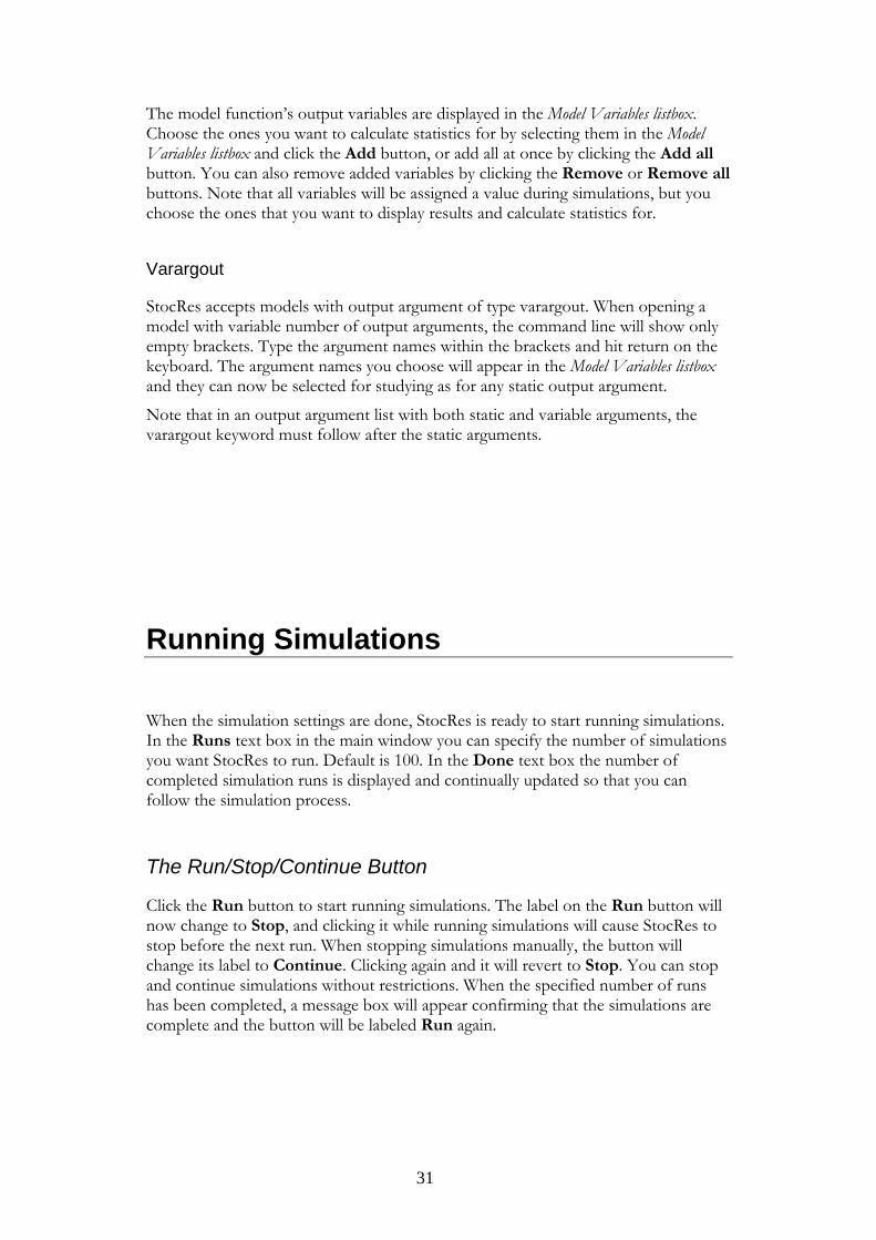
The model function’s output variables are displayed in the Model Variables listbox. Choose the ones you want to calculate statistics for by selecting them in the Model Variables listbox and click the Add button, or add all at once by clicking the Add all button. You can also remove added variables by clicking the Remove or Remove all buttons. Note that all variables will be assigned a value during simulations, but you choose the ones that you want to display results and calculate statistics for.

Varargout

StocRes accepts models with output argument of type varargout. When opening a model with variable number of output arguments, the command line will show only empty brackets. Type the argument names within the brackets and hit return on the keyboard. The argument names you choose will appear in the Model Variables listbox and they can now be selected for studying as for any static output argument.

Note that in an output argument list with both static and variable arguments, the varargout keyword must follow after the static arguments.

Running Simulations

When the simulation settings are done, StocRes is ready to start running simulations. In the Runs text box in the main window you can specify the number of simulations you want StocRes to run. Default is 100. In the Done text box the number of completed simulation runs is displayed and continually updated so that you can follow the simulation process.

The Run/Stop/Continue Button

Click the Run button to start running simulations. The label on the Run button will now change to Stop, and clicking it while running simulations will cause StocRes to stop before the next run. When stopping simulations manually, the button will change its label to Continue. Clicking again and it will revert to Stop. You can stop and continue simulations without restrictions. When the specified number of runs has been completed, a message box will appear confirming that the simulations are complete and the button will be labeled Run again.

31

Simulation Report

When simulations are finished, you can create a simulation report. It will contain the following data:

• Date and time for report generation

• Path and name of the model file

• Number of simulation runs completed

• Total time for the simulations

• Time when simulations was finished

Select Generate Report from the Functions menu. A dialog box will appear allowing you to choose the name of the file you want to put the report in. The report will be saved as an ASCII text file.

Analyzing Results

StocRes features a number of tools for analyzing data from simulations. In addition to the statistics that are calculated, visualization is possible in graphs. You can also apply any built-in function or your own function to the results.

Displayed Statistics

Statistics will be calculated and displayed for the simulations that were made before StocRes was stopped. When continuing, simulation results will be added to and statistics will be recalculated after the next stop.

StocRes has two different display views. Toggle between them by selecting either View Summary or View Details from the View menu. In the View Summary mode, a list of results for all variables is visible. In the View Details mode only one variable is visible at a time. The result is shown with higher precision and in addition a histogram is displayed. If results for more than one variable have been produced, you can change between the results for the different variables by choosing the variable you want to study from the Select variable list.

32

Statistic Settings

To set confidence level and percentile, select Statistics from the Settings menu. The statistics settings dialog then appears. It is also possible to specify whether confidence intervals should be one- or two-sided, and if they should be to the left or to the right if one-sided.

Statistic Settings dialog.

Click OK when you have made your settings, or Cancel to close the dialog without doing any changes. Note that you can change the statistics settings also after having done simulations. Calculated measures will then change automatically to the new settings.

Plots

StocRes offers some built in plots to be created from simulation data:

• Scatter Plot

• Histogram

• Histogram of All

From the Functions menu, select Plot in New Figure and the plot you want to create. The plot will appear in a new figure that can be further formatted (see the MATLAB documentation).

To create a scatter plot, select the variable you want to have on the x-axes in the results frame (in View Summary mode, select variable by marking it in the results listbox, and in View Details mode, select it from the popup list), and the variable you want on the y-axes in the Plot variable against popup. Then select Scatter Plot from Plot in New Figure in the Functions menu.

33

Histograms are created with the data from the variable selected in the results frame by selecting Histogram from the Plot in New Figure menu.

Histogram. StocRes plot functions open in a new figure where they can be further enhanced.

Histograms for all variables can be created in the same figure. Select Histogram of All to do this. Each variable will be displayed with a separate color in the figure.

Other kinds of graphs can also be created, either by issuing a plotting command from the Define Function dialog (see “Applying Other MATLAB Functions” p.13),

34

or by exporting the variable to MATLAB’s base workspace and continue working with it outside of StocRes (see “Export Data to the Base Workspace” p.14).

Applying Other MATLAB Functions

Analyzing results from the simulations is not restricted to the built-in functions available in StocRes. You can also apply any other function to the results.

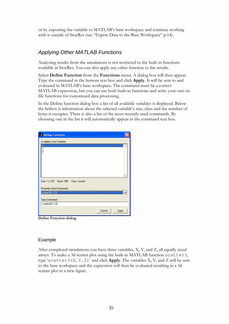
Select Define Function from the Functions menu. A dialog box will then appear. Type the command in the bottom text box and click Apply. It will be sent to and evaluated in MATLAB’s base workspace. The command must be a correct MATLAB expression, but you can use both built-in functions and write your own m-file functions for customized data processing.

In the Define function dialog box a list of all available variables is displayed. Below the listbox is information about the selected variable’s size, class and the number of bytes it occupies. There is also a list of the most recently used commands. By choosing one in the list it will automatically appear in the command text box.

Define Function dialog.

Example

After completed simulations you have three variables, X, Y, and Z, all equally sized arrays. To make a 3d scatter plot using the built-in MATLAB function scatter3, type ‘scatter3(X,Y,Z)’ and click Apply. The variables X, Y, and Z will be sent to the base workspace and the expression will then be evaluated resulting in a 3d scatter plot in a new figure.

35

Using Other Programs for Analysis and Presentation

It is possible to use other programs and utilities than MATLAB for data processing and presentation of the results. MATLAB offers several external interfaces. For instance, you can export your data to Microsoft Excel using ActiveX and DDE (see the MATLAB documentation). There are two ways to get your simulation data out of StocRes:

• Send it to the base workspace (see “Export Data to the Base Workspace”, p.36

• Write your own function to export the data (see “Applying Other MATLAB Functions”, p.35

Once the simulation data is in the base workspace you can take advantage of MATLAB’s data exporting capabilities (see the MATLAB documentation).

Saving and Loading

Simulation results can be saved for later use. StocRes saves the simulation results and the state it is in to a MATLAB *.mat file. Loading this file will restore StocRes to the state it was in when saved. It is then possible to continue simulations and/or using analysis tools and other features of StocRes.

To save results, select Save Results from the File menu and choose the file you want to save in from the dialog box that appears. Load the results back and restore the state by selecting Load Results from the File menu and choose the file you want to load. An error message will appear if the file does not contain data saved by StocRes.

If you want to save only the results for use outside StocRes, export the results to the MATLAB base workspace and save it from there (see the MATLAB documentation for saving workspace variables).

Export Data to the Base Workspace

StocRes is intended for running simulations and providing basic analysis. If you want to do a more extensive analysis of the simulation data, you can send the results to MATLAB’s base workspace, where it can be further processed, saved or exported to other programs such as Microsoft Excel.

To export the simulation results to the base workspace, select Send to Base from the File menu. Simulation results will be assigned to the variable srdata in the base

36

workspace. In case the output is strictly numeric, srdata will be a numeric array; otherwise it will be a cell array.

37

38

Appendix B

Wanda ParmEst for MATLAB User Documentation version 1

39

40

Wanda ParmEst for MATLAB

• Installation and Requirements 43

• What is ParmEst? 43

• The Main Window 45

• Starting and Quitting 46

• The Model File 46

• Connecting to a Model 50

• Running Simulations 54

• Analyzing Results 55

• Saving and Loading 60

41

42

Installation and Requirements

Wanda ParmEst for MATLAB requires MATLAB version 6 or later and is operating system independent. There are no other hardware requirements than those for MATLAB.

Since Wanda StocRes for MATLAB is a pure MATLAB application, it requires no explicit installation. Unpack the Wanda package in the directory where you would like to have the programs reside and edit the Startup File for MATLAB to include the directory in the MATLAB path (see the MATLAB documentation).

What is ParmEst?

ParmEst is a program for parameter estimation and statistical analysis of estimates in stochastic CSS models.

ParmEst uses a bootstrapping approach to estimate parameters and works in two phases. In the first phase, a deterministic model is fitted against system observations to produce an estimate of the parameter. The deterministic model is evaluated for a first guess on the parameter value (which must be supplied by the user). An objective function squares the difference between the output from the deterministic model and the system observations and sums the squares. A simplex optimizer is used to find the minimum of the objective function and hence the parameter value that minimizes the difference with the system. This parameter value is then the estimate. In the second phase, the estimate is transferred to the stochastic model, a replica of the deterministic model, but with stochastics built into it. The stochastic model is run once producing an output against which the deterministic model is fitted to produce an estimate. This is repeated N times giving a set of N estimates. Statistic measures can then be calculated based on these N samples to provide an idea to the quality of the estimate from phase one.

Statistical measures include: average, standard deviation, min, max, confidence interval, and percentile. ParmEst can also visualize results in forms of scatter plots and histograms, and take full advantage of MATLAB’s extensive capabilities.

43

Example

Assume that we want to calculate the decaying rate of a radioactive isotope (here called lambda). The dynamic model describing the decay is the well known negative exponential function, where lambda is the decaying rate or the intensity of the process and y is the number of atoms not yet decayed in a compound:

dydt = -lambda*y.

A Least Mean Square algorithm can be used to fit the model against the system observation and produce an estimate for lambda. Because the atoms have a stochastic behavior, decaying randomly, the decay in the compound which we have observed will not follow the mathematical model exactly but show some variations. This means that since we have only one observation that we can use, the estimate will be somewhat unsure. To get an idea of how good our estimate is, we can make our model stochastic and simulate it a number of times, each time fitting the deterministic model to the stochastic and thus producing many estimates for which we can calculate variations.

The stochastic model has the same structure as the deterministic one, but introduces Poisson distributed randomness. In the deterministic model, lambda is the decaying rate as if decay was deterministic and perfectly smooth. In the stochastic model, the decaying rate is stochastic and can be modeled as a Poisson process. The flow rate can be held constant during a short time period, dt. The number of atoms decaying during this time period will then be Po(lambda*y*dt) and the stochastic model will consequently have the following flow rate:

dydt = -(Poisson(lambda*y*dt))/dt

By repeatedly simulating the stochastic model and fitting the deterministic model to it each time, we get a number of estimates who, due to the stochastic properties of the mode,l varies slightly. Thus, variations around the estimate we produced in phase one can be calculated and we get an idea of how good the estimate is and how much we can expect it to vary in the real world.

44

The Main Window

a b c d e f g h i a – Plot variable against popup, see “Analyzing Results”

b – Menus – easy to reach functions c – Status line – information on status d – Number of runs – set number of simulation runs, see “Running Simulations”

e – Number of runs done – follow the progress f – Results – view results of simulations directly, see “Analyzing Results”

g – Opened file – the model file currently simulated

h – Run/Stop/Continue button – control simulations, see “Running Simulations”

i – Reset button – start over, see “Running Simulations”

45

Starting and Quitting

Starting ParmEst

To run ParmEst you must first run MATLAB and the directory containing the ParmEst files must be on the MATLAB path, or be the current directory. Type ‘parmest’ in the MATLAB command window to start ParmEst. This will cause ParmEst’s main window to appear on the screen, and its home directory will be added to the MATLAB path.

Quitting ParmEst

Quit ParmEst by selecting Exit from the File menu, or by clicking the close box in the ParmEst main window. ParmEst quits immediately without issuing a warning message. Simulation results that have not been saved will be lost. Plots created from the ‘Plots’ menu will remain after ParmEst has been quit.

Some settings and preferences will be saved by ParmEst in the file parmestini.mat when quitting.

The Model File

A ParmEst model is comprised of one main function and five model components:

1. System observation

2. Deterministic model

3. Stochastic model

4. Objective function for phase one

5. Objective function for phase two

None of these functions can use variable number of input or output arguments.

46

Main Function

The main function has no input arguments and returns function handles for the five model components. It has no other purpose than to bring the various parts of the model together. The function handles returned are used during simulation.

System Observation Function

A model includes one or more observations of the system. An observation is a time series of data, e.g. values of the studied parameters. In the first phase, the squared difference between the output from the deterministic model and the system is minimized. The system observation function returns the system observation as a matrix. It is then passed to the objective function together with the output from the deterministic model.

Deterministic Model

The deterministic model describes the continuous system without stochastics implemented. ParmEst expects a function representing the system. The deterministic model function must take the estimated parameters as input arguments, and return an output that corresponds to the system observation.

Stochastic Model

The stochastic model has the same dynamic structure as the deterministic model, but has stochastics implemented. It takes the parameter values from phase one as input arguments and returns a stochastic output. Because of its stochastic properties it is preferable to build this model using the Euler approximation.

Objective Functions

Two objective functions are needed, one for each phase. They take two vectors as input, square the element-wise difference between them and return the sum of the squared differences. The two objective functions are then minimized by finding the smallest sum by testing for different parameter values.

47

The structure of a ParmEst model.

Example

This example of a ParmEst model describes a radioactive decay, e.g. a negative exponential function. The parameter that is of interest for estimation is the decaying rate, here called lambda. All parts of the model file (system observations, deterministic and stochastic models, and objective functions) reside as subfunctions to the main function.

The system function, called sys_decay, returns an array with system observations that are stored in a mat-file and hence must be loaded.

Both the deterministic and stochastic models use the Euler approximation to project the trajectory. Using MATLAB’s built-in ode solvers could give unexpected results because of the stochastic properties of the model. It is also substantially faster to use a simpler algorithm.

Objective functions are needed to minimize the difference between the system and the deterministic model in phase one, and the difference between the stochastic and the deterministic models in phase 2.

function [sysh,deth,stoh sysminh,stominh] = decay % WANDA ParmEst demo model of radioactive decay % using the Euler approximation. % % Returns the following function handles: % - sysh system function % - deth deterministic model % - stoh stochastic model % - sysminh objective function for phase one % - stominh objective function for phase two % % Parameter for the deterministic and stochastic % models is lambda, the decaying rate.

48

sysh = @sys_decay; deth = @det_decay; stoh = @sto_decay; sysminh = @sysmin_decay; stominh = @stomin_decay; %--- System ---------------------------------------- function Y = sys_decay sysdata = load('decay_sysdata', 'Y'); Y = sysdata.Y; %--- Deterministic Function ------------------------ function y1 = det_decay(lambda) Y(1:100) = 100; % Initialize for k=2:(100) X = lambda*Y(k-1); % Flow rate Y(k) = Y(k-1)-X*dt; % Update end %--- Stochastic Function --------------------------- function Y = sto_decay(lambda) Y(1:100) = 100; % Initialize for k=2:(100) X = Poisson(lambda*Y(k-1)*dt)/dt; % Flow rate Y(k) = Y(k-1)-X*dt; % Update end %--- System Minimizing Function -------------------- function S = sysmin_decay(x,y) A1 = x-y; A2 = A1.^2; S = sum(A2); %--- Stochastic Model Minimizing Function ---------- function S = stomin_decay(x,y) A1 = x-y; A2 = A1.^2; S = sum(A2);

49

Connecting to a Model

Select Connect to Model ... from the File menu. Choose the model file and click OK. The Model Settings dialog box will now appear. It is a tabbed dialog box with three tabs:

1. General – Settings for model components and simplex optimizer

2. Deterministic Model – Settings for the deterministic model and estimated parameters

3. Stochastic Model – Additional settings for the stochastic model

Recently used files are available in Recent Files under the File menu. It is a convenient shortcut to open files recently used. The selected file will open and the settings dialog will appear.

Click OK when all settings have been made to leave the Model Settings dialog and keep the settings made. Click Cancel to leave without saving the settings. The Help button will display help for ParmEst in the Help Browser.

The General Tab

In the General tab, you can specify which function represents which model. To the left there are five popup menus, one for each model component. ParmEst’s default behavior is set the functions in the same order as the function handles returned by the model main function. If this is not the case, then select the correct functions representing each model component in the popups.

1. In the general tab there are also some settings for the simplex optimizer and the number of system observations.

2. Max number of iterations – maximum number of iterations the simplex optimizer is allowed to perform during one simulation run.

3. Max number of function evaluations – maximum number of function evaluations the simplex optimizer is allowed to perform during one simulation run.

4. Termination tolerance – termination tolerance on minimized variable

5. Number of system observations – number of observations in the system

1-3 are used by the simplex optimizer and passed directly to it. 4 is used when calculating confidence intervals.

50

The Deterministic Model Tab

The Deterministic Model tab is where you specify which function arguments that are the parameters to be minimized. All arguments in the model are displayed in the Parameter Name popup list, and each one of these must be defined either as a constant or as a parameter to be minimized.

To define an argument as a constant, specify the value in the Constant/Start value box and click Define. The value you specified will appear as an input argument in the Command Line Equivalent textbox at the bottom of the tab.

To define an argument as a parameter that the function will be minimized for, enter a start value in the Constant/Start value textbox. Then check the Estimate parameter checkbox and select the corresponding variable in the stochastic model in the Corresponding stochastic parameter popup list. Click Define to complete the definition. The start value will appear as an input argument in the Command line equivalent textbox.

To see the help file for the deterministic model function, click File Help. The help text is displayed in the MATLAB Help Browser. If the model function is a subfunction, the help text for the parent function will be displayed.

51

a

b

c

d

e

f

a – Parameter name popup – Select input parameters b – Constant/Start value textbox – Specify start values for the simplex optimizer c – Corresponding stochastic parameter textbox – Estimate a parameter and send it automatically to the stochastic model d – Define button

e – File help button – view help for the model file f – Command line equivalent – overview how the model is called

The Stochastic Model Tab

In the Stochastic Model tab you can specify constant values for input arguments. If an argument has been defined as a corresponding parameter to an estimated parameter, the Constant textbox will read ESTIMATED and no further definition can be made of that argument. A constant value for the stochastic model is defined in the same way as for the deterministic model.

The help for the stochastic model, if it exists, can be seen in the MATLAB Help Browser if you click File Help.

52

ParmEst can automatically send seeds to input arguments in the stochastic model. Leave the Constant/Start value textbox empty and check the Send seed checkbox before you click Define.

A new seed is automatically produced for each simulation run, but not for each time step. ParmEst uses a generator function to produce the seeds. This function can be specified after the settings for the model has been completed and has the following syntax:

seed = seedGenerator seed = seedGenerator(p1,p2,…,pn)

where seed is the seed, seedGenerator is the name of the function, and p1,p2,…,pn are input arguments.

In the Settings menu, select Seed Generator. This will display a dialog box with to text fields. Specify the name of the function that shall produce the seed in the first field. If the function has any input arguments, specify them as a comma separated list in the second field.

Seed Generator dialog

53

Running Simulations

When the settings for the model are done, ParmEst is ready to start running simulations. In the Runs textbox you can specify the number of simulations you want ParmEst to run in the second phase. Default is 100. In the Done textbox the number of completed simulation runs is displayed and continually updated so that you can follow the simulation process.

Parmest will first run phase one, in which the deterministic model is fitted against the system observation. This results in estimates of selected parameters, which are automatically transferred to the stochastic model for phase two.

If you want to run phase one only, then set the number of runs to 0. ParmEst will then stop before starting phase two and will not calculate any statistic measures. You can continue and run phase two by specifying a positive number of runs for phase two and then click the Run button.

In phase two, ParmEst will run the stochastic model once and then fit the deterministic model to the resulting output. This will be repeated for the number of times specified in the Runs box, producing a set of estimates. Statistics will then be calculated for these estimates.

The Run/Stop/Continue Button

Click the Run button to start running simulations. The label on the Run button will now change to Stop, and clicking it while running simulations will cause ParmEst to stop before the next run.

When stopping simulations manually, the button will change its label to Continue. Clicking again and it will revert to Stop. You can stop and continue simulations without restrictions. When the specified number of runs has been completed, a message box will appear confirming that the simulations are complete and the button will be labeled Run again.

Generate Simulation report

When simulations are finished, you can create a simulation report. It will contain the following data:

• Date and time for report generation

• Path and name of the model file

• Number of function evaluations in phase one

• Time for simulations in phase one

• Number of completed simulation runs in phase two

• Number of function evaluations in phase two

54

• Time for simulations in phase two

• Time when simulations was finished

Select Generate Report from the Functions menu. A dialog box will appear allowing you to choose the name of the file you want to put the report in. The report will be saved as an ASCII text file.

Analyzing Results

ParmEst features a number of tools for analyzing data from simulations. In addition to the statistic measures that are calculated, visualization is possible in a variety of graphs. You can also apply any built-in MATLAB function or your own function to the results.

Displayed Statistics

Statistics will be calculated and displayed for the simulations that were made before ParmEst was stopped. When continuing, simulation results will be added to and statistics will be recalculated after the next stop.

ParmEst has two different display views. Toggle between them by selecting either View Summary or View Details from the View menu. In the View Summary mode, a list of results for all estimated parameters is visible. In the View Details mode only one parameter is visible at a time. The result is shown with higher precision and in addition a histogram is displayed. If results for more than one variable have been produced, you can change between the results for the different variables by choosing the variable you want to study from the Select variable list.

Statistic Settings

To set confidence level and percentile, select Statistics from the Settings menu. The statistics settings dialog then appears. It is also possible to specify whether confidence intervals should be one- or two-sided, and if they should be to the left or to the right if one-sided.

55

Click OK when you have made your settings, or Cancel to close the dialog without doing any changes. Note that you can change the statistics settings also after having done simulations. Calculated measures will then change automatically to the new settings.

Plots

ParmEst offers some built in plots to be created from the simulation results data:

Plot of System Data and Deterministic Model

• Scatter Plot

• Histogram

• Histogram of All

From the Functions menu, select Plot in New Figure and the plot you want to create. The plot will appear in a new figure that can be further formatted (see the MATLAB documentation).

Plot displays a graph of the system observation(s) data together with a graph of the deterministic model evaluated using the estimate from phase one.

56

To create a scatter plot, select the variable you want to have on the x-axes in the results frame (in View Summary mode, select variable by marking it in the results listbox, and in View Details mode, select it from the popup list), and the variable you want on the y-axes in the Plot variable against popup. Then select Scatter Plot from Plot in New Figure in the Functions menu.

57

Histograms are created with the data from the variable selected in the results frame by selecting Histogram from the Plot in New Figure menu.

Histograms for all variables can be created in the same figure. Select Histogram of All to do this. Each variable will be displayed with a separate color in the figure.

Other kinds of graphs can also be created, either by issuing a plotting command from the Define Function dialog (see “Applying Other MATLAB Functions” p.28), or by exporting the variable to MATLAB’s base workspace and continue working with it outside of ParmEst (see “Export data to the Base Workspace” p.30).

Applying Other MATLAB Functions

Analyzing results from the simulations is not restricted to the built-in functions available in ParmEst. You can also apply any other function to the results.

Select Define Function from the Functions menu. A dialog box will then appear. Type the command in the bottom textbox and click Apply. It will be sent to and evaluated in MATLAB’s base workspace. The command must be a correct MATLAB expression, but you can use both built-in functions or write your own m-file functions for customized data processing.

In the Define function dialog box a list of all available variables is displayed. Below the listbox is information about the selected variable’s size, class and the number of bytes it occupies. There is also a list of the most recently used commands. By choosing one in the list it will automatically appear in the command textbox.

58

Example

After completed simulations you have three variables, X, Y, and Z, all equally sized arrays. To make a 3d scatter plot using the built-in MATLAB function scatter3, type ‘scatter3(X,Y,Z)’ and click Apply. The variables X, Y, and Z will be sent to the base workspace and the expression will then be evaluated resulting in a 3d scatter plot appearing in a new figure.

Using Other Programs for Analysis and Presentation

It is possible to use other programs and utilities than MATLAB for data processing and presentation of the results. MATLAB offers several external interfaces. For instance, you can export your data to Microsoft Excel using ActiveX and DDE (see the MATLAB documentation). There are two ways to get your simulation data out of ParmEst:

• Send it to the base workspace (see “Export Data to the Base Workspace” p.60

• Write your own function to export the data (see “Applying Other MATLAB Functions” p.58

Once the simulation data are in the base workspace you can take advantage of MATLAB’s data exporting capabilities (see the MATLAB documentation).

59

60

Saving and Loading

Simulation results can be saved for later use. ParmEst saves the simulation results and the state it is in to a MATLAB *.mat file. Loading this file will restore ParmEst to the state it was in when saved. It is then possible to continue simulations and/or using analysis tools and other features of ParmEst.

To save results, select Save Results from the File menu and choose the file you want to save in from the dialog box that appears. Load the results back and restore the state by selecting Load Results from the File menu and choose the file you want to load. An error message will appear if the file does not contain data saved by ParmEst.

If you want to save only the results for use outside ParmEst, export the results to the MATLAB base workspace and save it from there (see the MATLAB documentation on saving workspace variables).

Export Data to the Base Workspace

ParmEst is intended for estimating parameters, running simulations and providing basic analysis. If you want to do a more extensive analysis of the simulation data, you can send the results to MATLAB’s base workspace, where it can be further processed, saved or exported to other programs such as Microsoft Excel.

To export the simulation results to the base workspace, select Send to Base from the File menu. Simulation results will be assigned to the variable pedata in the base workspace. pedata will be a numeric array.