Wal-Mart, Oligopsony Power and Entry: an Analysis of Local Labor Markets

by

Alessandro Bonanno

Assistant Professor of Agricultural Economics

Department of Agricultural Economics and Rural Sociology The Pennsylvania State University

207-D Armsby Building University Park, PA16802-5600

Tel: (814) 863-8633 Fax: (814) 865-3746

Email: abonanno@psu.edu

Selected Paper prepared for presentation at the 2009 AAEA & ACCI Joint Annual Meeting in Milwaukee, WI, July 26–28, 2009

Copyright 2009 by A. Bonanno. All rights reserved. Readers may make verbatim copies of this document for non-commercial purposes by any means, provided that this copyright notice appears on all such copies.

1

Wal-Mart, Oligopsony Power and Entry: an Analysis of Local Labor Markets

Abstract

Wal-Mart, the largest retailer worldwide, has been suspected of exercising market power over input providers, both merchandise suppliers and workers. However, in spite of a growing body of literature investigating the beneficial economic impact of the company through its price-lowering effect, research analyzing the company’s economic impact over input suppliers is limited. This paper presents a general framework which can be used to investigate Wal-Mart’s market power over input suppliers, vis-à-vis a variation in input productivity, focusing on homogenous intermediate goods supplied locally. The model is general enough to account for incumbents’ reaction to Wal-Mart’s entry resulting in exit, entry and changes in the production technology. A simplified version of the theoretical model is tested using data on local labor markets. Preliminary results show Wal-Mart having a wage lowering effect due mainly to the increased productivity of labor, while the increase in oligopsony power counts only for 15% of such effect.

Key words: Wal-Mart, oligopsony, entry, wages

JEL: L13, L81, J42

2

Wal-Mart, Oligopsony Power and Entry: an Analysis of Local Labor Markets

1. Introduction

Wal-Mart, the largest retailer worldwide, has reshaped the American economic

environment in ways that go beyond triggering structural changes in the retailing industry

(Basker, Klimek and Hoang Van 2008). One of the main concerns regarding the company’s

expansion is that its beneficial impact on consumers through low prices (Basker 2005b; Basker

and Noel forthcoming; Cleary and Lopez 2008; Hausman and Liebtag 2007), may be generated

not only through the company’s efficient logistic system1 but also via market power over input

suppliers, these being both merchandise suppliers (Lynn 2006) and workers (Bonanno and Lopez

2008).

Wal-Mart’s alleged market power over suppliers has become an issue attracting the

attention of both economists and opinion leaders. If, on the one hand, the company’s so-called

“squeeze” of suppliers can be supported by several anecdotal cases (see Bianco 2007), on the

other hand, the issue may be much more extensive. Foyer (2007), for example, argues that

suppliers who sell their goods to Wal-Mart may be forced out of business not directly because of

the company’s requests for low prices, but also because other retailers do not accommodate

suppliers’ requests of higher prices since they are competing with Wal-Mart themselves. Another

indirect impact of Wal-Mart on input suppliers comes from the augmented competitive pressure

that the company creates by increasing imports and outsourcing from less developed countries.2

1 Financial Times has described Wal-Mart as “an operation whose efficiency is the envy of the world’s storekeepers (Edgecliffe–Johnson, 1999). Wal-Mart logistic management is destined to become even more efficient with wide use of the new Radio Frequency Identification (RFID) technology to manage in-store stocks (The Economist, 6/16/2006). 2 Basker and Hoang Van (2008) estimate that Wal-Mart’s growth along with the reduction in input cost, due to tariff reductions, account for 40% of the growth of US imports from China in the period 1998-2004.

3

Despite the relevance of understating the impact of the phenomenon, to date there is little

formal analysis aiming to measure the extent of Wal-Mart’s impact on suppliers. Foyer (2007)

points out that one of the main difficulty in undertaking such analysis is to find an appropriate

definition of the relevant market, since Wal-Mart’s suppliers are spread across the U.S. and

abroad. Two additional issues make this type of analysis even harder to be pursued successfully:

1) the limited availability of extensive and accurate data on input markets, and 2) the lack of

access to Wal-Mart data.

This paper presents a framework that circumvents these limitations proposing a model to

measure Wal-Mart’s shift in retail oligopsony power over suppliers of homogenous goods

produced locally. The rationale behind the model is that, by focusing on locally supplied inputs,

one could measure the change in market conduct in geographically limited retail markets as Wal-

Mart’s store openings occur. Also, thanks to the assumption of homogeneity, only one market-

level price for each intermediate good is needed, which allows to overcome problems connected

with data availability.

The model accounts for three scenarios: 1) a (Wal-Mart) pre-entry scenario; 2) a post

entry scenario where incumbent firms do not react to Wal-Mart’s entry and; 3) a second, more

complete, post-entry scenario in which retailers’ entry, exit and changes in the technology used

by incumbents are taken into account.3

As a preliminary first application of this model, the impact of Wal-Mart’s entry on retail

wages is analyzed. Using a simplified version of the theoretical model and county-level data

results suggest that 1) Wal-Mart’s depressive effect over per-capita retail earnings does exist, and

3 As Khanna and Tice (2000) pointed out that two of the strategies that retailers implemented as a consequence of Wal-Mart entry were to divest some of their less efficient establishments or to invest in new technology. Both these factors, along with entry from large retailer may push efficiency up.

4

2) that the main source of this effect is the increased productivity of labor, while the increase in

oligopsony power accounts for only 15%.

2. A General Model of Oligopsony with Entry

The model draws from Azzam’s (1997) oligopsony model, Lopez, Azzam and Lirón-

España (2002) oligopoly model and its extension in Cleary and Lopez (2008)4. Differently from

those analyses, this paper derives explicitly the sources of variation in the equilibrium price of

the input consistently with the entry of a large firm (i.e. Wal-Mart) and it allows for changes in

the incumbents’ composition as a consequence of the company’s entry, as well as for the

adoption of technologies that resemble that of Wal-Mart.

2.1 A general model of oligopsony

Consider a local retail market where Wal-Mart does not operates. Assume there are N

retailers, each using a vector of K homogeneous inputs to deliver a bundle of goods sold at

competitive prices. Assume the kth input is supplied locally, meaning that the structure (and

conduct) of the retail firms located in a given area will have an impact on the market price for the

input. The supply of k is defined as:

(1) ( ),k k kX f w= Z

where wk is input k’s market price and Zk is a vector of supply shifters. Consider retailer i, where

{ }1,...,i N= maximizes profits by choosing the optimal amount of inputs:

4 To date, only two studies have adopted a structural approach to investigate Wal-Mart’s conduct, Cleary and Lopz (2008) and Bonanno and Lopez (2008). In particular, Cleary and Lopez (2008) have used a simple structural model in part similar to that discussed in this paper, where Wal-Mart entry is considered as an exogenous shock that shifts traditional retailers’ conduct in the Dallas Forth-Worth milk market.

5

(2) ( )1

max , ,i

K

i i i ik kk

R t p x wπ=

= −∑x

x

where ( )iR ⋅ is retailer i revenue function, xi is a vector of inputs used by i, t is a time indicator

and p is a vector of competitive prices common to all retailers. Assume that, for simplicity,

retailers do not have market power over inputs other than the k-th; this assumption allows ease of

exposition and could be easily released. Assuming that the revenue function is continuous and

differentiable in inputs’ quantity one has the following optimal condition for the k-th input: 5

(3) ( ) ( ) ,

,

1, , i i ki ik

i k

sR t pw

x

θη

+∂= −

∂x

;

where i ,,

i ki k

k

xs

X= is retailer’s i k-th input share,

1k

k

dX

dw Xη = is the semi-elasticity of input supply

of k (η >0), ,

,

Nj k

ij i i k

dx

dxθ

≠

=∑ it the i-th retailer’s conjectural variation in the k-th input, and

( ) ,.i i kR x∂ ∂ represents the marginal revenue product of k .

Assuming for smplicity that the N retailers adopt the same technology; the production

function for the bundle of goods sold by retailer i is assumed to be continuous, homogenous and

twice differentiable in the inputs, and takes a quadratic functional form:

(4) ( )1 1 1 1

1,

2

K K K K

i i k ik kl ik il kt ikk k l k

Y t x x x x tα α α= = = =

= + +∑ ∑∑ ∑x .

To maintain the exposition simple, the special case of only two inputs, namely Xk and Xl

will be considered, where k is the input over which retailers show market power, l that for which

the market is assumed to be competitive. Following Lopez, Azzam and Lirón-España (2002),

5 The market price for any of the other imports will be defined by the following condition

( ),

, , /k i i i k

w R t p x− −= ∂ ∂x indicating that the price of an intermediate good will be equal to its marginal revenue

product.

6

differentiating (4) with respect to ,i kx replacing this expression into (3), multiplying both sides of

(3) by ,i k kx X , standardizing output prices to 1, and summing across N one has:

(5) ( )1

;kk k kk k k kt kl l kl

Hw H X t X Gα α α α

η+ Θ

= + + + −

where 2

1

N

k iki

H s=

=∑ is the Herfindahl index of retail concentration in the k-th input market,

1

N

lk il iki

G s s=

=∑ is the Generalized Herfindahl index proposed by Shi, Chavas and Stiegert (2008)

to measure cross-market effects of imperfect competition on bundle pricing; Xk (Xl ) represent

the equilibrium quantity of input k (l) used in retailing and 1 2

1

N

k ik ii

H s θ−

=

Θ = ∑ is the industry-level

(weighted) equilibrium conjectural variation. 6

Manipulating (5), one can obtain the oligopsony version of Blair and Harris (1993)

Buying Power Index (BPI), or

(6) ( )1kk k

kk k

Hw MRPBPI

w wη+ Θ−= = − ;

where MRPk is the marginal revenue product of input k. The BPI measures the markdown, or

rather the percentage of input price, below the competitive level which retailers would pay to

suppliers. The BPI grows in magnitude as the demand for inputs becomes more concentrated and

as the input supply becomes more semi-elastic.

6 The reader should notice that ( )1 1 k kH H− ≤ Θ ≤ − . The limit values represent respectively the perfectly

competitive scenario ( )1,i iθ = − ∀ and the monopoly scenario 1, , ,i i k j k

i j

s s iθ −

≠

= ∀

∑ . An other value of interest

is 0Θ = ( )0,i iθ = ∀ , leading to a “0” conjecture Cournot oligopoly game outcome.

7

2.2 Wal-Mart’s entry

Consider a local market where Wal-Mart enters. This scenario treats the number and

composition of the incumbent retailers as fixed after Wal-Mart’s entry; in other words, this

scenario accounts for the short-run “shock” that occurs in the input market immediately after

Wal-Mart’s entry.7

Let the post-entry analogous of the firm-level equilibrium condition (3) for the N

retailers other than Wal-Mart be:

(7 - a) ( ) ( ) '

,

.

1, ,wm

i i i ki ik

i k

sR t pw

x

θ θη

+ +∂= −

∂x

;

where, ,

,

Nj k

ij i i k

x

xθ

≠

∂=

∂∑ ; ,

,

wm wm ki

i k

x

xθ

∂=

∂ for i=1,…N and ,'

, '

i ki k

k

xs

X= , where '

, ,1

N

k wm k i ki

X x x=

= +∑ .

Wal-Mart optimizing behavior is:

(7 - b) ( ) ( ) ,

,

1, , wm wm kwm wmk

wm k

sR t pw

x

θη

+∂= −

∂x

;

where ,

1 ,

Nj k

wmj xm k

x

xθ

=

∂=

∂∑ and ,, '

wm kwm k

k

xs

X= .

Wal-Mart’s technology is assumed to be represented by the same functional form as that

of other retailers; however, its parameterization cannot be the same, as the company is likely to

have a “superior” technology in terms of both input utilization, and logistic structure

(Edgecliffe–Johnson 1999). The marginal product of input k for both all retailers other than Wal-

Mart, and for Wal-Mart, respectively, are:

7 As this assumption would imply that Wal-Mart’s entry does not push competitors out of business or that it does not attract other retailers in the same geographic areas it is clearly very strong and not consistent with anecdotal evidence and empirical findings (Khanna and Tice 2000).

8

( )

( )

, , ,,

' ' ' ', , ,

,

, , ,

,(8 a)

,(8 b)

i ik kk i k kl i k i l kt

k i

wm wmk kk wm k kl wm k wm l kt

k wm

k k kk kk wm k kl kl wm k wm l kt kt

y tx x x t

x

y tx x x t

x

x x x t

α α α α

α α α α

α β α β α β α β

∂− = + + +

∂

∂− = + + + =

∂

+ + +

x

x

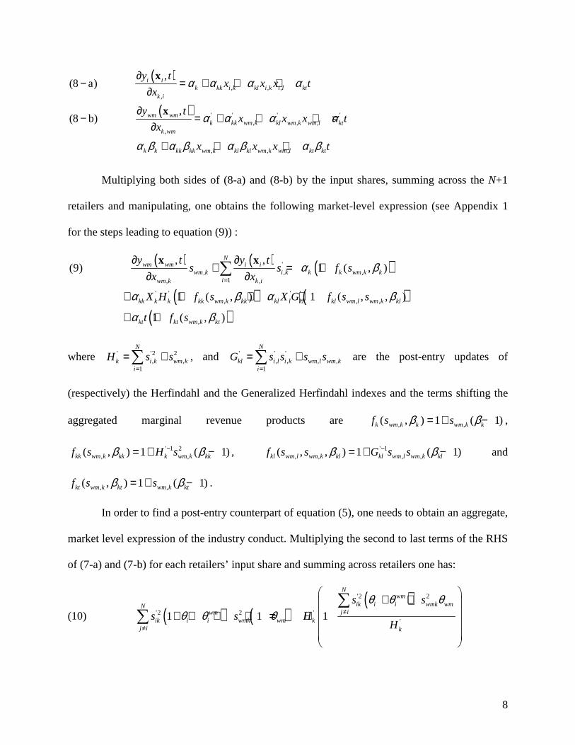
Multiplying both sides of (8-a) and (8-b) by the input shares, summing across the N+1

retailers and manipulating, one obtains the following market-level expression (see Appendix 1

for the steps leading to equation (9)) :

( ) ( ) ( )

( ) ( )( )

', , ,

1, ,

' ' ' ', , ,

,

, ,(9) 1 ( , )

1 ( , ) 1 ( , , )

1 ( , )

Nwm wm i i

wm k i k k k wm k kiwm k k i

kk k k kk wm k kk kl l kl kl wm l wm k kl

kt kt wm k kt

y t y ts s f s

x x

X H f s X G f s s

t f s

α β

α β α β

α β

=

∂ ∂+ = +

∂ ∂

+ + + +

+ +

∑x x

where ' '2 2, ,

1

N

k i k wm ki

H s s=

= +∑ , and ' ' ', , , ,

1

N

kl i l i k wm l wm ki

G s s s s=

= +∑ are the post-entry updates of

(respectively) the Herfindahl and the Generalized Herfindahl indexes and the terms shifting the

aggregated marginal revenue products are , ,( , ) 1 ( 1)k wm k k wm k kf s sβ β= + − ,

' 1 2, ,( , ) 1 ( 1)kk wm k kk k wm k kkf s H sβ β−= + − , ' 1

, , , ,( , , ) 1 ( 1)kl wm l wm k kl kl wm l wm k klf s s G s sβ β−= + − and

, ,( , ) 1 ( 1)kt wm k kt wm k ktf s sβ β= + − .

In order to find a post-entry counterpart of equation (5), one needs to obtain an aggregate,

market level expression of the industry conduct. Multiplying the second to last terms of the RHS

of (7-a) and (7-b) for each retailers’ input share and summing across retailers one has:

(10) ( ) ( )( )'2 2

'2 2 ''

1 1 1

Nwm

ik i i wmk wmNj iwm

ik i i wmk wm kj i k

s s

s s HH

θ θ θθ θ θ ≠

≠

+ + + + + + = +

∑∑

9

Assuming that post-entry input shares for each of the i-firms is proportional to the pre-

entry ones by a factor equal to 1/2δ , so that

(11) ' '2 2 2 2 2, ,

1 1

N N

k i k wmk i k wmk k wmki i

H s s s s H sδ δ= =

= + = + = +∑ ∑ ;

which leads to the market-level conduct expression (whose derivation is reported in Appendix

2):

(12) ( ) ( ) ( )' 2 2 ' ', ,1 1 1 ( )

Nwm

ik i i wm k wm k wm wm kj i

s s H sθ θ θ≠

+ + + + = + Θ + Θ∑ ;

where 1 2 2 ' 1 2, , , ,

1 1

( ) ( )N N

wm wmwm wm k k i k i wm k k i k i i wm

i i

s H s s H sθ θ θ θ− −

= =

Θ = − + − ∑ ∑ represents the shift in

oligopsonistic conduct with the entry of Wal-Mart.

Combining (12) and (9), normalizing for prices, one obtains the market-level input-price

setting equation with an entrant:

( ) ( )( ) ( )

( )

' ', ,

' ', , ,

,

(13) 1 ( , ) 1 ( , )

1 ( , , ) 1 ( , )

' 1 ( )

k k k wm k k kk k k kk wm k kk

kl l kl kl wm l wm k kl kt kt wm k kt

wm wm k

w f s X H f s

X G f s s t f s

H s

α β α β

α β α β

η

= + + + +

+ + + +

+ Θ + Θ−

from which it is easy to observe that the post-entry BPI is:

(14) ( ) ,' ( )' 1 wm wm k

k k

H sHBPI

w wη ηΘ+ Θ

= − − ;

where the second term on the RHS represents the shift in oligopsony power as consequence of

Wal-Mart’s entry.

10

2.3 Post-entry scenario with entry, exit and productivity shifts

The third scenario considers that, as consequence of Wal-Mart’s entry, some incumbent

retailers will be driven out of business (exit the market), while others enter the market. The

number of firms in the market at an arbitrary period t subsequent to that of Wal-Mart’s entry is

defined as�tN ; �'tN represents the number of firms operating in the market at time t which were

active before Wal-Mart entered, so that� �'ttN N− indicates the number of entrants after Wal-Mart

entry occurred (new entrants).

Once again, the short-run profit maximizing conditions (where inputs’ quantity is the

choice variable), for the �tN retail firms, and Wal-Mart, respectively, are

(15-a)

( )

�

( ) �( ), ,

,,, ,

, ,

11, , , ,

tNj k wm k

wmi ki i i i kj i i k i ki i i i

kk i k i

x xs

sx xR t p R t pw

x x

θ θ θη η

≠

∂ ∂+ + + + +∂ ∂∂ ∂ = − = −

∂ ∂

∑x x

ɶɶ

and

(15-b)

( )

�

( ) �( ),

,,1 ,

, ,

11, , , ,

tNj k

wm kwm kwm wmj wm kwm wm wm wm

kk wm k wm

xs

sxR t p R t pw

x x

θ θη η

=

∂+ + +∂∂ ∂ = − = −

∂ ∂

∑x x

ɶɶ

where �� � �' '

,

,

t t tN N N Nj k k

ij i k ii k i

x x

x xθ

− −

≠ ≠

∂ ∂= −∂ ∂∑ ∑ and �

� � �' ',

1 1,

t t tN N N Nj k k

wmj kwm k wm

x x

x xθ

− −

= =

∂ ∂= −∂ ∂∑ ∑ , while the new input shares

are defined as , ,i k i k ks x X=ɶ ɶ and , ,wm k wm k ks x X=ɶ ɶ where �

, ,1

tN

k wm k i ki

X x x=

= +∑ɶ .

In proceeding with the aggregation of (15-a) and (15-b), one should multiply, again, both

sides of each equation for the respective market shares ,i ksɶ for the retail firms other than Wal-

11

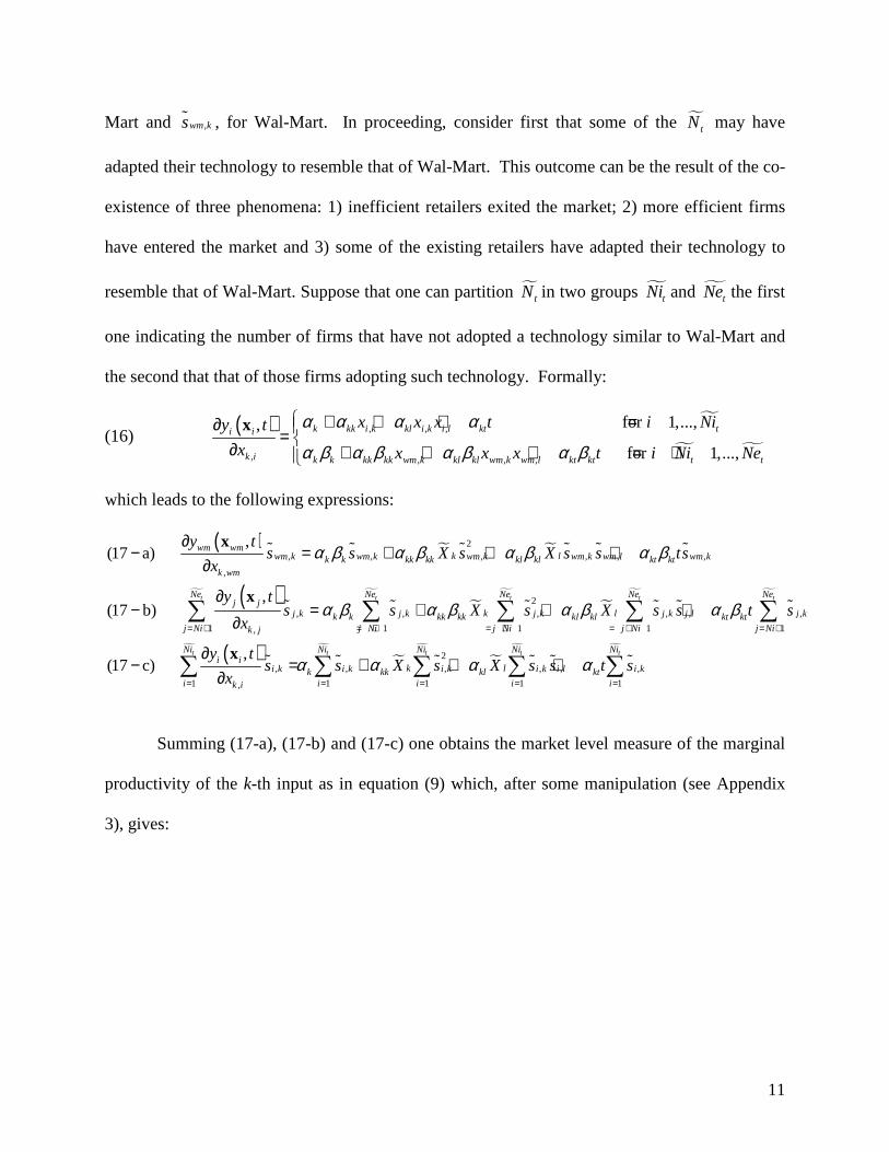
Mart and ,wm ksɶ , for Wal-Mart. In proceeding, consider first that some of the �tN may have

adapted their technology to resemble that of Wal-Mart. This outcome can be the result of the co-

existence of three phenomena: 1) inefficient retailers exited the market; 2) more efficient firms

have entered the market and 3) some of the existing retailers have adapted their technology to

resemble that of Wal-Mart. Suppose that one can partition �tN in two groups �tNi and �tNe the first

one indicating the number of firms that have not adopted a technology similar to Wal-Mart and

the second that that of those firms adopting such technology. Formally:

(16) ( ) �

� �

, , ,

, , , ,

for 1,...,,

for 1,...,

k kk i k kl i k i l kt ti i

k i k k kk kk wm k kl kl wm k wm l kt kt t t

x x x t i Niy t

x x x x t i Ni Ne

α α α α

α β α β α β α β

+ + + =∂ = ∂ + + + = +

x

which leads to the following expressions:

( ) � �

( )� �

�

�

�

�

2, , , , , ,

,

2, , , , ,

1 1 1 1,

,(17 a)

,(17 b)

t t t t

wm wmk lwm k wm k wm k wm k wm l wm kk k kk kk kl kl kt kt

k wm

Ne Ne Ne Nej j

k lj k j k j k j k j lk k kk kk kl kl ktj Ni j Ni j Ni j Nik j

y ts s X s X s s ts

x

y ts s X s X s s

x

α β α β α β α β

α β α β α β α= + = + = + = +

∂− = + + +

∂

∂− = + + +

∂∑ ∑ ∑ ∑

x

x

ɶ ɶ ɶ ɶ ɶ ɶ

ɶ ɶ ɶ ɶ ɶ

�

( )� �

�

�

�

� �

,

1

2, , , , , ,

1 1 1 1 1,

,(17 c)

t

t t t t t

Ne

j kktj Ni

Ni Ni Ni Ni Nii i

k li k i k i k i k i l i kk kk kl kti i i i ik i

t s

y ts s X s X s s t s

x

β

α α α α

= +

= = = = =

∂− = + + +

∂

∑

∑ ∑ ∑ ∑ ∑x

ɶ

ɶ ɶ ɶ ɶ ɶ ɶ

Summing (17-a), (17-b) and (17-c) one obtains the market level measure of the marginal

productivity of the k-th input as in equation (9) which, after some manipulation (see Appendix

3), gives:

12

( ) ( ) ( )

�( )� � �( )� �

, , ,

1 1, , ,

,, , ,

,, , ,

,, ,(18)

1 ( , ) ( , , ) ( , , )

1 ( , ) ( , , ) ( , , )

Ni Nej jwm wm i i

wm k i k j k

i j Nik wm k i k j

j kk k wm k k k wm k wm k k k t k

k k j kkk kk wm k kk kk wm k wm k kk kk t kk

lkl

y ty t y ts s s

x x x

f s g s h Ne s

X H f s g s h Ne s

X G

α β λ β β

α β λ β β

α

= = +

∂∂ ∂+ + =

∂ ∂ ∂

+ + +

+ + + +

+

∑ ∑xx x

ɶ ɶ ɶ

ɶ

ɶ

�( )�( )

, ,, , , , , ,

,, , ,

1 ( , , ) ( , , , ) ( , , , )

1 ( , ) ( , , ) ( , , )

kl j k j lkl wm l wm k kl kl wm l wm k wm k wm l kl kl t kl

j kkt kt wm k kt kt wm k wm k kt kt t kt

f s s g s s h Ne s s

t f s g s h Ne s

β λ λ β β

α β λ β β

+ + +

+ + + +

ɶ ɶ

ɶ

where the (.) (.)f s are described in section 2.2, and the other marginal revenue product shifters

(again, output prices are assumed to be standardized to 1) are:

(18-a) , , , ,( , , ) ( 1)k wm k wm k k wm k wm k kg s sλ β λ β= − ;

(18-b) �

�

, ,

1

( , , ) ( 1) ;tNe

j k j kk t k kj Ni

h Ne s sβ β= +

= − ∑ɶ ɶ

(18-c) , ,( , , )kk wm k wm k kkg s λ β � �1 12 2

, , , ,( 1) (2 )( 1)k kk kk wm k wm k wm k kk wm kH H s H sβ λ λ β− −

= − − + + −ɶ

;

(18-d) � �

�

1 2, ,

1

( , , ) ( 1)tNe

kj k j kkk t kk kkj Ni

h Ne s H sβ β−

= +

= − ∑ɶ ɶ ;

(18-e) , , , ,( , , , )kl wm l wm k wm k wm l klg s s λ λ β =

� �1 1

, , , , , , , ,( 1) ( )( 1)kl klkl kl wm k wm l wm k wm l wm k wm l kl wm k wm lG G s s G s sβ λ λ λ λ β− −

− − + + + −ɶ

;

(18-f) � �

�

1, , , ,

1

( , , , ) ( 1) ;tNe

j k j l kl j k j lkl t kl klj Ni

h Ne s s G s sβ β−

= +

= − ∑ɶ ɶ ɶ ɶ

(18-g) , , , ,( , , ) ( 1)kt wm k wm k kt wm k wm k ktg s sλ β λ β= − ; and

(18-h) �

�

, ,

1

( , , ) ( 1)tNe

j k j kkt t kt ktj Ni

h Ne s sβ β= +

= − ∑ɶ ɶ .

kHɶ and klGɶ are the updated Herfindahl and Generalized Herfindahl Indexes:

(19-a) �

�

2 2 ', ,

1

N

k i k wm k k ki

H s s H H=

= + = +∑ ɶ ɶ

ɶ.

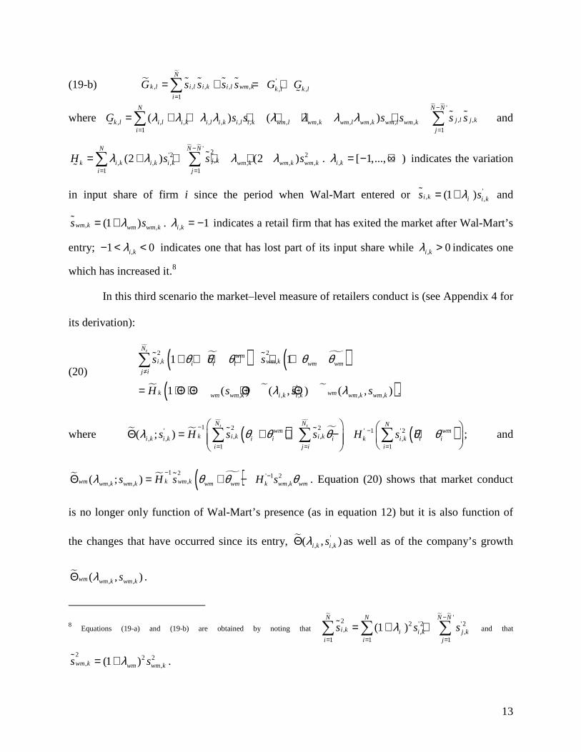
13

(19-b) ��

', , , , , , ,

1

N

k l i l i k i l wm k k l k li

G s s s s G G=

= + = +∑ ɶ ɶ ɶ ɶ

ɶ

where � � '

, ,, , , , , , , , , , , , ,1 1

( ) ( )N N N

j l j kk l i l i k i l i k i l i k wm l wm k wm l wm k wm l wm ki j

G s s s s s sλ λ λ λ λ λ λ λ−

= =

= + + + + + +∑ ∑ ɶ ɶɶ

and

� � ' 2'2 2,, , , , , ,

1 1

(2 ) (2 )N N N

j kk i k i k i k wm k wm k wm ki j

H s s sλ λ λ λ−

= =

= + + + +∑ ∑ ɶɶ

. , [ 1,..., )i kλ = − +∞ indicates the variation

in input share of firm i since the period when Wal-Mart entered or ', ,(1 )i k i i ks sλ= +ɶ and

, ,(1 )wm k wm wm ks sλ= +ɶ . , 1i kλ = − indicates a retail firm that has exited the market after Wal-Mart’s

entry; ,1 0i kλ− < < indicates one that has lost part of its input share while , 0i kλ > indicates one

which has increased it.8

In this third scenario the market–level measure of retailers conduct is (see Appendix 4 for

its derivation):

(20)

�( )�

�( )� � �( )

2 2, ,

', , , , ,

1 1

1 ( ) ( , ) ( , ) .

tNwm

i k wm ki i i wm wmj i

k wmwm wm k i k i k wm k wm k

s s

H s s s

θ θ θ θ θ

λ λ

≠

+ + + + + +

= + Θ + Θ + Θ + Θ

∑ ɶ ɶ

where � �

�

( )�

� ( )1 2 2' ' 1 '2, ,, , ,

1 1

( ; )t tN N N

wm wmk i k i ki k i k i i i k i k i i

i j i i

s H s s H sλ θ θ θ θ θ− −

= = =

Θ = + + − + ∑ ∑ ∑ɶ ɶ ; and

� � �( )1 2 ' 1 2,, , ,( ; ) kwm wm kwm k wm k wm wm k wm k wms H s H sλ θ θ θ

− −Θ = + −ɶ . Equation (20) shows that market conduct

is no longer only function of Wal-Mart’s presence (as in equation 12) but it is also function of

the changes that have occurred since its entry, � ', ,( , )i k i ksλΘ as well as of the company’s growth

�, ,( , )wm wm k wm ksλΘ .

8 Equations (19-a) and (19-b) are obtained by noting that

� � � '2 2 '2 '2, , ,

1 1 1

(1 )N N N N

i k i i k j ki i j

s s sλ−

= = =

= + +∑ ∑ ∑ɶ and that

2 2 2, ,(1 )wm k wm wm ks sλ= +ɶ .

14

The resulting the market-level input-price setting equation is:

�( )� � �( )� � �

,, , ,

,, , ,

,, , , , , ,

(21) 1 ( , ) ( , , ) ( , , )

1 ( , ) ( , , ) ( , , )

1 ( , , ) ( , , , ) ( ,

j kk k k wm k k k wm k wm k k k t k

k k j kkk kk wm k kk kk wm k wm k kk kk t kk

l kl j kkl kl wm l wm k kl kl wm l wm k wm k wm l kl kl t

w f s g s h Ne s

X H f s g s h Ne s

X G f s s g s s h Ne s

α β λ β β

α β λ β β

α β λ λ β

= + + +

+ + + +

+ + + +

ɶ

ɶ

ɶ( )�( )

� � �( )

,

,, , ,

, , , , ,

, , )

1 ( , ) ( , , ) ( , , )

1 ( ) ( , ) ( , );

j l kl

j kkt kt wm k kt kt wm k wm k kt kt t kt

k wmwm wm k i k wm k wm k wm k

s

t f s g s h Ne s

H s s s

β

α β λ β β

λ λη

+ + + +

+ Θ + Θ + Θ + Θ−

ɶ

ɶ

which results in the following expression of the BPI:

(22) � ( ) � � � � �'

, , , , ,( ) ( , ) ( , )1 k k kk wmwm wm k i k i k wm k wm kk

k k k k

H s H s H sHBPI

w w w w

λ λη η η η

Θ Θ Θ+ Θ= − − − − ,

stating that the post-entry markdown with full adjustments is function of: 1) the shift in baseline

conduct as consequence of the company entry, ',( )wm wm ksΘ ; 2) the variations in other retailers’

composition, � , ,( , )i k i ksλΘ ; and 3) growth of Wal-Mart’s presence � , ,( , )wm wm k wm ksλΘ .

Also, it is easy to note that equation (21) nests equation (13), which in turn nests equation

(5). Similarly equation (22) nests (14) which nests (6), fact which will result to be useful in the

empirical implementation of the model.

3. An application to local labor markets.

The model illustrated in the previous section is used to determine the sources and the

extent of Wal-Mart’s depressive effect on retail workers’ wages. Since retail labor is rather

homogenous, mainly unskilled and it is also supplied locally (as unskilled labor has limited

mobility), the retail labor markets represent a good case study to test the validity of the model.

Also the widespread presumption that Wal-Mart lowers retail wages has triggered a debate

15

concerning the company’s effect on the condition of workers in the retailing industry, fact which

makes the analysis interesting on its own merit.

Besides being the largest retailer in the World, Wal-Mart is also the largest private

employer with a workforce of 1.36 million people, (Wal-Mart Inc. United States Operational

Datasheet, May 2007) exceeding public education employment (Neumark, Zhang and Ciccarella,

2008). Wal-Mart has often been accused of paying low wages and shifting health care costs onto

local and state governments. Shils and Taylor (1997), report that half of Wal-Mart “associates”

in the 1990’s received wages only slightly above the prevailing Federal minimum wage of $4.25

an hour and that many of the company’s full time employees were food stamps recipients.9

The impact of Wal-Mart on workers, highlighted by anti-Wal-Mart movements and the

company’s crackdown against unionization,10 is an increasing concern of local policymakers,

who have already tried to pass regulations to target “big-box” retailers, Wal-Mart in particular, to

improve the conditions of their workers by obliging the company to pay both higher wages and

hourly benefits (e.g., Chicago’s ‘living wage’ ordinance)11 or to contribute to public healthcare

expenditures (The Maryland Fair Share Health Act).12

9 The company does provide its workers with other types of compensations: since 1971 Wal-Mart offers its own stocks to its associates based upon the profit growth of the company (Walton and Huey, 1992). 10 Wal-Mart is notoriously a “union free” environment, which has caused the major unions of retail workers to sponsor anti-Wal-Mart movements: for example Wal-Mart Watch is an organization that allegedly “monitors” Wal-Mart business practices founded by the Service Employees International Union (SEIU). WakeUpWalMart.com follows the same broad objectives as Wal-Mart Watch and is strongly connected with the United Food and Commercial Workers (UFCW). 11 On July 26, 2006 the Chicago City Council passed an ordinance requiring stores with more than 90,000 square feet and companies grossing more than $1 billion annually to pay a minimum wage of $10 by 2010 along with hourly benefits worth at least $3. The ordinance was to affect only “big-box” retailers, slowing down the penetration of Wal-Mart in the Chicago area, and would have included not only Wal-Mart but also Kmart, Toys R’ Us and Target which were already operating in the area. 12 In January 2006 the Maryland State Assembly passed the Maryland Fair Share Health Act (SB 790) which would have required employers with more than 10,000 employees to spend 8% of their payroll on medical benefits or pay the difference in taxes that would have gone to the Maryland Medicaid fund. At the time of the bill Wal-Mart employed nearly 17,000 individuals in the state and was the only known company of such size that did not meet that spending requirement (Wagner, 2006).

16

Academics have also shown increasing interest in investigating the impact of Wal-Mart

on retail workers. The existing empirical literature investigating these effects has mainly treated

Wal-Mart’s presence as a shock to local labor markets (e.g. Basker, 2005a; Hicks, 2005;

Neumark et al., 2008; and Dube, Lester and Eidlin, 2007). A common feature of these studies is

that the labor market is not modeled explicitly, raising doubts as to the economic interpretation

of their findings; for instance, a negative effect of the company on wages and/or employment

could be attributed either to market power over workers or to an increase in the productivity of

non-labor inputs.

These analyses have produced so far mixed evidence of positive and negative effects due

primarily to differences in the empirical strategy used to correct for the endogeneity of Wal-

Mart’s location decision and the data used. Regarding the effect of Wal-Mart on employment

alone, Basker (2005a) finds that although Wal-Mart has a small positive effect on county-level

retail employment, it reduces wholesale employment but does not affect sectors outside the scope

of the company’s goods and services. She used planned openings instead of actual openings to

correct for store location endogeneity and did not measure the impact on wages. Hicks (2005),

using quarterly workforce indicators data, found similar positive effects for the company’s entry

on Pennsylvania counties’ employment and labor turnover without, however, addressing the

problem of endogenous store location.

Regarding the effects of Wal-Mart on earnings, Neumark et al. (2008) found a negative

impact of the company on both county-level retail employment and earnings; they estimated that

for each store opened, retail employment fell by 3.2 % and retail earnings dropped by about

2.7%. These authors used interactions of time and distance from Wal-Mart headquarter in

17

Benton County, Arkansas, to correct for the endogeneity of Wal-Mart’s store location.13 Similar

instruments for Wal-Mart’s location are used by Dube, Lester and Eidim (2007) who found that

Wal-Mart expansion causes a reduction in retail workers’ earnings estimated to be between 0.5

and 0.9%. They also established that Wal-Mart’s effect in decreasing wages it is not due to

differences in workforce characteristics, but it is primarily associated with increased rents for the

company.

A first attempt to measure the anticompetitive behavior of Wal-Mart over retail workers

is that of Bonanno and Lopez (2008) who modeled Wal-Mart as a dominant firm with wage

setting power. Although their work is limited in scope, focusing on area where the company

operates and disregarding its location decision, their results found Wal-Mart does having

monopsony power over workers, with varying magnitude across the country, with the maximum

degree of market power estimated for rural areas in southern central states, exceeding 6%.

4. Empirical Model

The empirical model illustrated below is a restricted version of the conceptual one and

draws from the empirical work of Cleary and Lopez (2008) and Bonanno and Lopez (2008). As

the data used in its implementation are at the county level, the “local” area of interest will be a

county. The key estimable equation of the empirical model does not account for exit/entry

adjustment but it provides an exemplification of equation (13), where the number of Wal-Mart

stores in a given area (county) at time t, itWM , is used as a proxy of Wal-Mart input share and its

functions:

13 Although distance and time are truly exogenous variables and the motivation behind the use of them as instruments of Wal-Mart presence comes directly form the description of the company’s expansion strategy by the same Wal-Mart founder’ Sam Walton in his autobiography (Walton and Huey, 1992) their identification strategy is heavily criticized by Basker (2006) in a technical working paper.

18

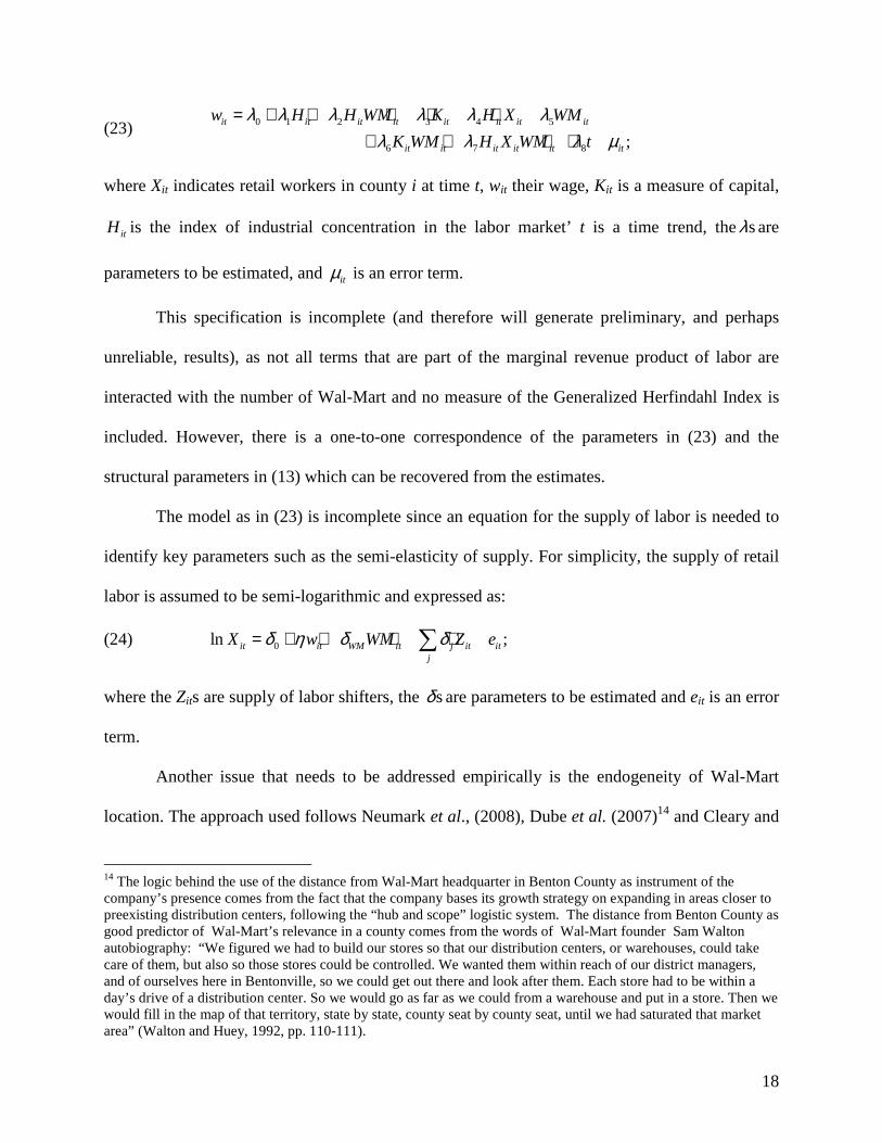
(23) 0 1 2 3 4 5

6 7 8 ;it it it it it it it it

it it it it it it

w H H WM K H X WM

K WM H X WM t

λ λ λ λ λ λλ λ λ µ

= + + + + ++ + + +

where Xit indicates retail workers in county i at time t, wit their wage, Kit is a measure of capital,

itH is the index of industrial concentration in the labor market’ t is a time trend, thesλ are

parameters to be estimated, and itµ is an error term.

This specification is incomplete (and therefore will generate preliminary, and perhaps

unreliable, results), as not all terms that are part of the marginal revenue product of labor are

interacted with the number of Wal-Mart and no measure of the Generalized Herfindahl Index is

included. However, there is a one-to-one correspondence of the parameters in (23) and the

structural parameters in (13) which can be recovered from the estimates.

The model as in (23) is incomplete since an equation for the supply of labor is needed to

identify key parameters such as the semi-elasticity of supply. For simplicity, the supply of retail

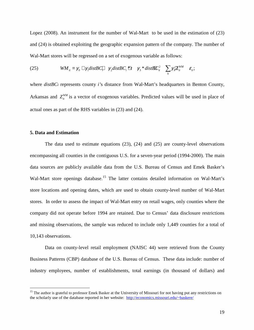
labor is assumed to be semi-logarithmic and expressed as:

(24) 0ln ;it it WM it j it itj

X w WM Z eδ η δ δ= + + + +∑

where the Zits are supply of labor shifters, the sδ are parameters to be estimated and eit is an error

term.

Another issue that needs to be addressed empirically is the endogeneity of Wal-Mart

location. The approach used follows Neumark et al., (2008), Dube et al. (2007)14 and Cleary and

14 The logic behind the use of the distance from Wal-Mart headquarter in Benton County as instrument of the company’s presence comes from the fact that the company bases its growth strategy on expanding in areas closer to preexisting distribution centers, following the “hub and scope” logistic system. The distance from Benton County as good predictor of Wal-Mart’s relevance in a county comes from the words of Wal-Mart founder Sam Walton autobiography: “We figured we had to build our stores so that our distribution centers, or warehouses, could take care of them, but also so those stores could be controlled. We wanted them within reach of our district managers, and of ourselves here in Bentonville, so we could get out there and look after them. Each store had to be within a day’s drive of a distribution center. So we would go as far as we could from a warehouse and put in a store. Then we would fill in the map of that territory, state by state, county seat by county seat, until we had saturated that market area” (Walton and Huey, 1992, pp. 110-111).

19

Lopez (2008). An instrument for the number of Wal-Mart to be used in the estimation of (23)

and (24) is obtained exploiting the geographic expansion pattern of the company. The number of

Wal-Mart stores will be regressed on a set of exogenous variable as follows:

(25) 20 1 2 3* * ;WM

it i i it h it ith

WM distBC distBC t distBC Zγ γ γ γ γ ε= + + + + +∑

where distBCi represents county i’ s distance from Wal-Mart’s headquarters in Benton County,

Arkansas and WMitZ is a vector of exogenous variables. Predicted values will be used in place of

actual ones as part of the RHS variables in (23) and (24).

5. Data and Estimation

The data used to estimate equations (23), (24) and (25) are county-level observations

encompassing all counties in the contiguous U.S. for a seven-year period (1994-2000). The main

data sources are publicly available data from the U.S. Bureau of Census and Emek Basker’s

Wal-Mart store openings database.15 The latter contains detailed information on Wal-Mart’s

store locations and opening dates, which are used to obtain county-level number of Wal-Mart

stores. In order to assess the impact of Wal-Mart entry on retail wages, only counties where the

company did not operate before 1994 are retained. Due to Census’ data disclosure restrictions

and missing observations, the sample was reduced to include only 1,449 counties for a total of

10,143 observations.

Data on county-level retail employment (NAISC 44) were retrieved from the County

Business Patterns (CBP) database of the U.S. Bureau of Census. These data include: number of

industry employees, number of establishments, total earnings (in thousand of dollars) and

15 The author is grateful to professor Emek Basker at the University of Missouri for not having put any restrictions on the scholarly use of the database reported in her website: http://economics.missouri.edu/~baskere/

20

number of establishments belonging to nine employment size classes.16 Earnings per worker,

obtained by dividing total earnings by the number of employees, are used in place of wages. The

shifters used in the supply of labor equation are total labor force, unemployment rate (following

Hall, Henry and Pemberton, 1992) and the percentage of the county population belonging to

three age groups: between 15 and 24, 25 and 64 and over 65 years of age (to control for the

composition of the retailing supply of labor).17 In order to control for unobservables, the shifters

include also state-level fixed effects.

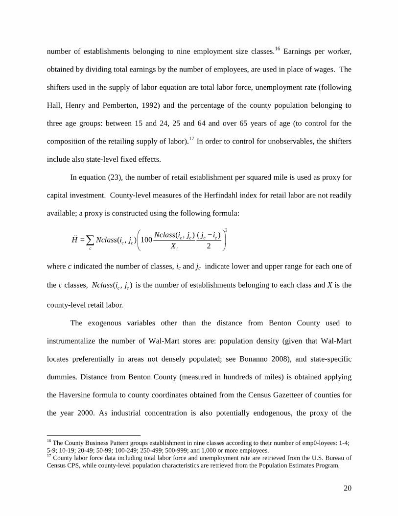
In equation (23), the number of retail establishment per squared mile is used as proxy for

capital investment. County-level measures of the Herfindahl index for retail labor are not readily

available; a proxy is constructed using the following formula:

2( , ) ( )

( , ) 1002

c c c cc c

c i

Nclass i j j iH Nclass i j

X

−=

∑⌣

where c indicated the number of classes, ic and jc indicate lower and upper range for each one of

the c classes, ( , )c cNclass i j is the number of establishments belonging to each class and X is the

county-level retail labor.

The exogenous variables other than the distance from Benton County used to

instrumentalize the number of Wal-Mart stores are: population density (given that Wal-Mart

locates preferentially in areas not densely populated; see Bonanno 2008), and state-specific

dummies. Distance from Benton County (measured in hundreds of miles) is obtained applying

the Haversine formula to county coordinates obtained from the Census Gazetteer of counties for

the year 2000. As industrial concentration is also potentially endogenous, the proxy of the

16 The County Business Pattern groups establishment in nine classes according to their number of emp0-loyees: 1-4; 5-9; 10-19; 20-49; 50-99; 100-249; 250-499; 500-999; and 1,000 or more employees. 17 County labor force data including total labor force and unemployment rate are retrieved from the U.S. Bureau of Census CPS, while county-level population characteristics are retrieved from the Population Estimates Program.

21

Herfindahl index is instrumentalized following Lopez, Azzam and Lirón-España (2002) by

regressing it on a set of exogenous variables such as the (distance) weighted average of the

lagged number of retail stores operating in a 100 miles radius from county i, an indicator variable

for rural counties (from and the County Typology Codes reported by the Economic Research

Service of the United States Department of Agriculture)18, and state dummies. Once all the

variables are operational and the instrument for the number of Wal-Mart stores available,

equations (23), (24), and the Herfindahl Index instrument are estimated via Three-Stage Least

Squares (3SLS).

7. Preliminary Results

The estimated parameters for equations (23) and (24) are reported in Table 1. The results

for the OLS used to instrumentalize the number of Wal-Mart stores and the Herfindahl index

equation are omitted for brevity. The estimated coefficients of the supply of retail labor show

that the semi-elasticity of retail labor supply is positive and significant, for an estimated

parameter of 0.1655, resulting, at the sample averages, in an elasticity of 2.3219. The results

support Neumark et al (2008) findings that as Wal-Mart expands, retail labor is impacted

negatively: the supply of labor shrinks in fact of approximately 0.6% for each store opened. The

behavior of the shifters is consistent with that of previous research (Bonanno and Lopez 2008):

the retail supply of labor grows with the size of the labor force, but it is not impacted by the rate

of unemployment; also individuals in the age group including high school/college students (15-

24) are more likely to actively seek job in retailing, being also more willing to accept part time

18 The distinction between rural and urban counties considers as “urban” those counties indicated as “metro” by the Bureau of Census and “rural” the remaining ones. Metro areas include central counties with urbanized areas of 50,000 or more residents, regardless of total area population. In addition, the Census “metro” classification includes outlying counties with commuting thresholds of 25 percent, with no metropolitan character requirement.

22

jobs and the flexibility required by retailing operations; individuals in the age group going from

25 to 64 are less likely to participate in the retailing supply of labor, while retirees (over 65 years

old) appear indifferent.

The estimates of the wage equation show the coefficient for the Herfindahl index being

positive, which suggests that retailers other than Wal-Mart show limited anti-competitive

behavior. As Wal-Mart’s presence increases, the market becomes more anti-competitive

(estimated coefficient for the interaction of the Herfindahl index with the number of Wal-Mart is

negative and significant being -2.5418). This suggests that Wal-Mart’s presence shift retailers

oligopsonistics’ conduct with respect to workers toward less competitive values. Also, it appears

that labor utilization becomes more efficient over time. Structural parameters are presented in

Table 2.

The estimated conduct parameters, as well as the BPIs and the impact of Wal-Mart’s

presence on wages (at the sample averages) are reported in Table 3. The value of the estimated

baseline conduct parameter is 0.2080, which is statistically different than zero only at the 10%

level. This provides evidence that retailers other than Wal-Mart have limited market power. The

presence of Wal-Mart causes a consistent increase in oligopsony power, with the average

industry conduct parameter doubling and reaching 0.4208. The BPI increases in magnitude with

Wal-Mart’s presence, going from a minimum of -0.13 % to a maximum of -0.59 % for each

store, which is consistent with the wage differential across counties with and without Wal-Mart

found by Dube et al. (2008) and in line with Bonanno and Lopez (2008) estimates of Wal-Mart’s

monopsony power in counties having only one Wal-Mart store.

At the sample averages, the estimated depressive effect of Wal-Mart on per capita retail

earnings through market power is approximately $ 444, which is only about 15% of the total

23

estimated depressive effect accounting also for the increasing productivity of labor as an

outcome of Wal-Mart’s presence, being approximately $ 3,000.

8. Concluding Remarks

Wal-Mart, the largest retailer worldwide, has been accused of being able to charge those

low prices which have catalyzed its success, not only through an efficient logistic system, but

also through the exertion of market power over input suppliers, both merchandise suppliers and

workers. Despite the company’s reach grows larger and with it the amount of control over its

suppliers, empirical research aimed at analyzing the anticompetitive behavior of Wal-Mart is

limited, mainly because of the difficulties in underpinning the relevant market of analysis and the

paucity of detailed data.

The model developed in this paper overcomes these issues proposing a framework apt to

investigate the anti-competitive behavior of the company over its suppliers, by focusing on

homogenous inputs supplied locally. The model is as such that the company’s entry has the

potential to shift retailers’ oligopsony power as well as the productivity of inputs. The model is

flexible as it allows for entry, exit and retailers’ adoption of technologies to match that of Wal-

Mart, nesting simpler, more restrictive, scenarios. A preliminary empirical use of the model to

local retail labor markets, show that up to 85% of any decrease in retail per capita earnings due

to Wal-Mart’s presence, comes from a decrease in the marginal revenue product of labor,

indicating only a small contribution of market power.

24

Table 1. Estimated Parameters and related statistics Coefficients St. Error T-ratios Supply of Retail Labor W 0.1655 0.0214 7.7390 NWM -0.5894 0.1229 -4.7970 Unemployment -0.0101 0.0069 -1.4640 Labor Force 6.02E-06 1.89E-07 31.8500 % 15-24 0.0196 0.0039 4.9930 % 25-64 -0.0162 0.0036 -4.4540 Over 65 -2.49E-05 3.28E-05 -0.7595 Constant 5.3156 0.3114 17.0700 Fixed Effect Wage Equation H 4.7846 0.2771 17.2600 H*WM -2.5418 0.4002 -6.3520 H*X -1.73E-05 5.56E-06 -3.1190 Capital 0.0246 0.0025 9.7840 NWM 2.5774 0.1128 22.8500 H*X*WM 1.79E-05 5.69E-06 3.1480 Capital*WM 0.0217 0.0042 5.1530 T 0.8378 0.0254 33.0200 Constant 9.4825 0.1104 85.8800 Supply Elasticity 2.3219 0.3000 59.8997 System R2 0.7283 Supply of Retail Labor R2 0.5503 Wage Equation R2 0.4499

25

Table 2. Structural Parameters

0kα λ= 9.4825

3klα λ= 0.0246

4kkα λ= -1.7E-05

5 01 /kβ λ λ= + 1.271806

6 31 /klβ λ λ= + 1.882114

7 41 /kkβ λ λ= + -0.03468 '

5 0ka λ λ= + 12.0599 '

6 3klα λ λ= + 0.0463 '

7 4kkα λ λ= + 6.00E-07

Table 3. Measures of Wal-Mart’s Impact on Wages Coefficients St. Error Wald-Stat* Conduct Parameters Θ 0.2080 0.1116 3.4707

WMΘ 0.4208 0.0857 24.1119 Impact of Wal-Mart on Wages Market Power -0.4442 0.0699 40.3428 Efficiency -2.6162 0.1124 541.9336 Total -3.0604 0.1644 346.4878

* For the Wald test the critical values of a2(1)χ are 3.84, 6.63 and 10.83

respectively for a 5%, 1% and 0.1 % significance level.

26

Reference

Azzam, A. 1997. “Measuring Market Power and Cost-Efficiency Effects of Industrial

Concentration” Journal of Industrial Economics 45,(4), 377-86.

Basker, E. 2005a. “Job Creation or Destruction? Labor Market Effects of Wal-Mart Expansion”

Review of Economics and Statistics 87, (1), 174-183

Basker, E. 2005b. "Selling a Cheaper Mousetrap: Wal-Mart's effect on retail prices," Journal of

Urban Economics 58, (2), 203-229

Basker, E. 2006. "When Good Instruments Go Bad" Unpublished Paper, University of Missouri

Department of Economics Working Paper 07-06. Available at

http://economics.missouri.edu/~baskere/papers/. Accessed 05/16/2007.

Basker, E. and M. D. Noel (forthcoming) “The Evolving Food Chain: Competitive Effects of

Walmart’s Entry into the Supermarket Industry.” Journal of Economics and Management

Strategy.

Basker, E. amd P. Hoang Van (2008) “Wal-Mart as Catalyst to U.S.-China Trade” University of

Missouri Department of Economics Working Paper 07-10. Available at

http://economics.missouri.edu/~baskere/papers/ Accessed 05/04/2009.

Basker. E,, S. Klimek and P. Hoang Van (2008) “Supersize It: The Growth of Retail Chains and

the Rise of the “Big Box” Retail Format” University of Missouri Department of

Economics Working Paper.

Bianco, A. (2007) “Wal-Mart: The Bully of Bentonville: How the High Cost of Everyday Low

Prices is Hurting America” Broadway Business Press.

Blair, R. D. and J. L. Harrison. 1993. “Monopsony: Antitrust Law and Economics”. Princeton

University press. Princeton. New Jersey.

27

Bonanno, A. 2008. An Empirical Investigation of Wal-Mart’s Expansion into Food Retailing.

Food Marketing Policy Center Research Report, N, 105. University of Connecticut,

Storrs, CT. Available at http://www.fmpc.uconn.edu/publications/reports.php.

Bonanno, A. and Lopez, R. A. 2008. Wal-Mart’s Monopsony Power in Local Labor Markets.

Food Marketing Policy Center Research Report, No. 103. University of Connecticut,

Storrs, CT. Available at http://www.fmpc.uconn.edu/publications/reports.php. Accessed

02/20/2008.

Cleary, R. and R. A. Lopez. 2008. “Does the Presence of Wal-Mart Cause Dallas/Fort Worth

Supermarket Milk Prices to Become More Competitive?” Food Marketing Policy Center

Research Report, No. 99. 28 pages. Available at

http://www.fmpc.uco\nn.edu/publications/reports.php . Accessed 01/31/2008.

Dube, A., T. W. Lester and B. Eidlin. 2007. “Firm Entry and Wages: Impact of Wal-Mart

Growth on Earnings throughout the Retailing Sector.” Working paper, Institute of

Research on Labor and Employment, University of California, Berkeley.

The Economist. “The Physical Internet - A Survey of Logistic” June, 16th, 2006.

Edgecliff-Johnson, A 1999. “A Friendly Store from Arkansas.” Financial Times June 19.

Foer. A. 2007. “Mr. Magoo Visits Wal-Mart: Finding the Right Lens for Antitrust.” Connecticut

Law Review; Special Issue – Breaking Up the Big Box: Trade Regulation and Wal-Mart,

May 4 (39).

Hall, S., G. B. Henry and M. Pemberton. 1992. “Testing a Discrete Switching Disequilibrium

Model of the UK Labour Market” Journal of Applied Econometrics 7 (1), 83-91.

28

Hausman, J. and E. S. Leibtag, 2004. “CPI Bias from Supercenters: Does the BLS Know That

Wal-Mart Exists?” NBER working paper series, Working Paper 10712.Available at

http://www.nber.org/papers/w10712. Accessed 06/10/2006.

Hausman, J., & Leibtag, E. S. (2007). Consumer benefits from increased competition in

shopping outlets: measuring the effect of Wal-Mart. Journal of Applied Econometrics, 22

(7) 1157-1177.

Hicks, M. J. 2005. “What Do Quarterly Workforce Dynamics Tell Us about Wal-Mart? Evidence

from New Stores in Pennsylvania.” 0511010. Econ WPA. Available at

http://ideas.repec.org/p/wpa/wuwpur/0511010.html. Accessed 09/10/2006.

Jia, P. (2008). What happens when Wal-Mart comes to town: an empirical analysis of the

discount retail industry. Econometrica, 76, (6) 1263-1316.

Khanna N. and S. Tice (2000) “Strategic responses of incumbents to new entry: The effect of

ownership structure, capital structure, and focus.” Review of Financial Studies 13 (2000),

pp. 749–779.

Lopez, R. A., A. Azzam, and C. Lirón-España. 2002. “Market Power and/or Efficiency:

A Structural Approach.” Review of Industrial Organization 20:115-126.

Lynn, B. C. 2006. “Breaking the Chain: The Antitrust Case Against Wal-Mart”. Harper’s

Magazine. July 2006. 29-36. Available at www.harpers.org. Accessed 11/12/2007.

Neumark, D., J. Zhang, and S. Ciccarella. 2008. “The Effects of Wal-Mart on Local Labor

Markets.” Journal of Urban Economics 63(2): 405-430.

Shils, E. B. and G. W. Taylor. 1997. “The Shils Report - Measuring the Economic and

Sociological Impact of the Mega-Retail Discount Chains on Small Enterprise in Urban,

29

Suburban and Rural Communities." Wharton School of Business, University of

PennsylvaniaAvailable at http://www.lawmall.com/rpa/rpashils.htm. Accessed 11/10/06.

Shi, Guanming Shi, J.P. Chavas, and K. Stiegert (2008) “An Analysis of Bundle Pricing: The

Case of the Corn Seed Market” Working Paper FSWP 2008-01, University of Wisconsin-

Madison. Available at http://www.aae.wisc.edu/fsrg 02/04/2009.

U. S. Bureau of Census, County Business Patterns Database: Various Years. Available at

http://www.census.gov/epcd/cbp/download/cbpdownload.html. Accessed 06/20/2006.

U. S. Bureau of Census, Gazetteer of Counties. 2000. Available at

http://www.census.gov/geo/www/gazetteer/places2k.html Accessed 06/20/2006.

U. S. Bureau of Census, Population Estimates Program: Various Years. Available at

http://www.census.gov/popest/estimates.php. Accessed 07/16/2006.

U. S. Department of Agriculture, Economic Research Service: Measuring Rurality: 2004

County Typology Codes. Available at

http://www.ers.usda.gov/Briefing/Rurality/Typology/Methods/ accessed 11/20/06.

Wagner, J. 2006. “Md. Legislature Overrides Veto on Wal-Mart Bill” The Washington

Post. January 13, Page A01

Wal-Mart Inc: United States Operational Data Sheet - May 2007. Available at

http://www.walmartfacts.com/articles/5025.aspx . Accessed 16/07/2007

Walton, S. and J. Huey. 1992. “Sam Walton, Made in America: My Story”, Doubleday

Publisher, New York City, New York.

30

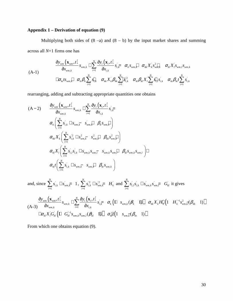
Appendix 1 – Derivation of equation (9)

Multiplying both sides of (8 –a) and (8 – b) by the input market shares and summing

across all N+1 firms one has

(A-1)

( ) ( ) ' ' 2 ', , , , , ,

1, ,

' ' '2 ' ' ' ', , , , , ,

1 1 1 1

, ,Nwm wm i i

wm k i k k wm k kk k wm k kl l wm l wm kiwm k i k

N N N N

kt wm k k k i k kk k kk i k kl kl l i l i k kt kt i ki i i i

y t y ts s s X s X s s

x x

ts s X s X s s t s

α α α

α α β α β α β α β

=

= = = =

∂ ∂+ = + +

∂ ∂

+ + + + +

∑

∑ ∑ ∑ ∑

x x

rearranging, adding and subtracting appropriate quantities one obtains

( ) ( ) ', ,

1, ,

' ', , , ,

1

' '2 2 2 2, , , ,

1

' ' ', , , , , , , ,

1

, ,(A 2)

Nwm wm i i

wm k i kiwm k i k

N

k i k wm k wm k k wm ki

N

kk k i k wm k wm k kk wm ki

N

kl l i l i k wm k wm l wm k wm l kl wm k wm li

y t y ts s

x x

s s s s

X s s s s

X s s s s s s s s

α β

α β

α β

=

=

=

=

∂ ∂− + =

∂ ∂

+ − + +

+ − + +

+ − +

∑

∑

∑

∑

x x

', , , ,

1

N

kt i k wm k wm k kt wm ki

t s s s sα β=

+

+ − + ∑

and, since ' ', ,

1

1N

i k wm ki

s s=

+ =∑ , '2 '2 ', ,

1

N

i k wm k ki

s s H=

+ =∑ and ' ' ' ' ', , , ,

1

N

i l i k wm k wm l kli

s s s s G=

+ =∑ it gives

(A-3)

( ) ( ) ( ) ( )

( ) ( )

' ' ' ' 1 2, , , ,

1, ,

' ' ' 1, , ,

, ,1 ( 1) 1 ( 1)

1 ( 1) 1 ( 1)

Nwm wm i i

wm k i k k wm k k kk k k k wm k kkiwm k i k

kl l kl kl wm k wm l kl kt wm k kt

y t y ts s s X H H s

x x

X G G s s t s

α β α β

α β α β

−

=

−

∂ ∂+ = + − + + −

∂ ∂

+ + − + + −

∑x x

From which one obtains equation (9).

31

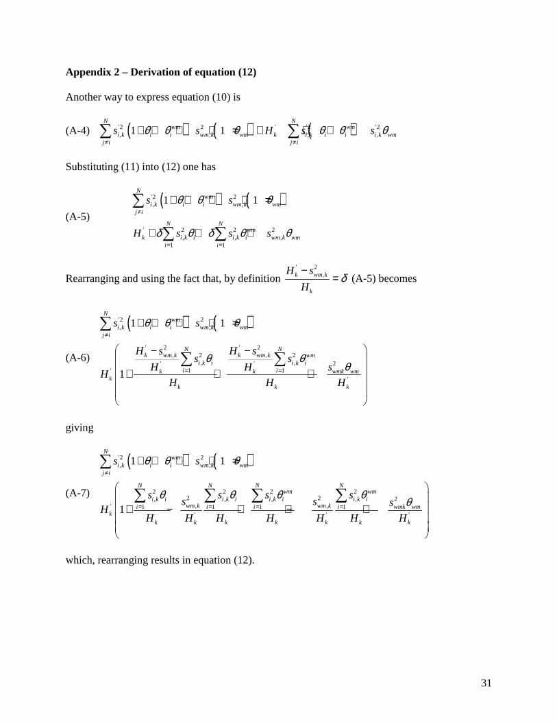
Appendix 2 – Derivation of equation (12)

Another way to express equation (10) is

(A-4) ( ) ( ) ( )'2 2 ' '2 '2, , , ,1 1

N Nwm wm

i k i i wm k wm k i k i i i k wmj i j i

s s H s sθ θ θ θ θ θ≠ ≠

+ + + + = + + +∑ ∑

Substituting (11) into (12) one has

(A-5) ( ) ( )'2 2

, ,

' 2 2 2, , ,

1 1

1 1N

wmi k i i wm k wm

j i

N Nwm

k i k i i k i wm k wmi i

s s

H s s s

θ θ θ

δ θ δ θ θ

≠

= =

+ + + + =

+ + +

∑

∑ ∑

Rearranging and using the fact that, by definition ' 2

,k wm k

k

H s

Hδ

−= (A-5) becomes

(A-6)

( ) ( )'2 2, ,

' 2 ' 2, ,2 2

, ,' ' 21 1'

'

1 1

1

Nwm

i k i i wm k wmj i

N Nk wm k k wm k wm

i k i i k ii ik k wmk wm

kk k k

s s

H s H ss s

H H sH

H H H

θ θ θ

θ θθ

≠

= =

+ + + + =

− − + + +

∑

∑ ∑

giving

(A-7)

( ) ( )'2 2, ,

2 2 2 22 2 2, , , ,

, ,' 1 1 1 1' ' '

1 1

1

Nwm

i k i i wm k wmj i

N N N Nwm wm

i k i i k i i k i i k iwm k wm ki i i i wmk wm

kk k k k k k k

s s

s s s ss s s

HH H H H H H H

θ θ θ

θ θ θ θθ

≠

= = = =

+ + + + =

+ − + + − +

∑

∑ ∑ ∑ ∑

which, rearranging results in equation (12).

32

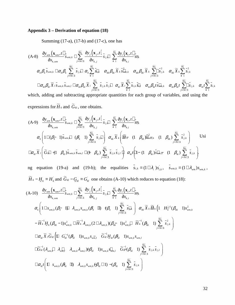
Appendix 3 – Derivation of equation (18)

Summing (17-a), (17-b) and (17-c), one has

( ) ( )� ( )�

� �

� �

�

�

�

�

, , ,

1 1, , ,

2 2 2, , , , , ,

1 1 1 1

,

,, ,(A-8)

t t

t t t t

Ne Nij jwm wm i i

wm k j k i k

j Ni ik wm k j k i

Ne Ni Ne Ni

k k kwm k j k i k wm k j k i kk k k k k kk kk kk kk kkj Ni i j Ni i

l wm kkl kl

y ty t y ts s s

x x x

s s s X s X s X s

X s

α β α β α α β α β α

α β

= + =

= + = = + =

∂∂ ∂+ + =

∂ ∂ ∂

+ + + + +

+

∑ ∑

∑ ∑ ∑ ∑

xx xɶ ɶ ɶ

ɶ ɶ ɶ ɶ ɶ ɶ

ɶ �

�

�

� � �

, , , , , , , ,

1 1 1 1

t t t tNe Ni Ne Ni

l lwm l j k j l i k i l wm k j k i kkl kl kl kt kt kt kt ktj Ni i j Ni i

s X s s X s s ts t s t sα β α α β α β α= + = = + =

+ + + + +∑ ∑ ∑ ∑ɶ ɶ ɶ ɶ ɶ ɶ ɶ ɶ

which, adding and subtracting appropriate quantities for each group of variables, and using the

expressions for� kH and � klG , one obtains.

( ) ( )� ( )�

�

� �

�

� �

, , ,

1 1, , ,

2 2, , , ,

1 1

,, ,(A-9)

1 ( 1) ( 1) (1 ) (1 )

(1 )

t t

t t

Ne Nij jwm wm i i

wm k j k i k

j Ni ik wm k j k i

Ne Ne

k kwm k j k wm k j kk k k kk kk kkj Ni j Ni

l klkl kl

y ty t y ts s s

x x x

s s X H s s

X G s

α β β α β β

α β

= + =

= + = +

∂∂ ∂+ + =

∂ ∂ ∂

+ − + − + + − + −

+ + −

∑ ∑

∑ ∑

xx xɶ ɶ ɶ

ɶ ɶ ɶ ɶ

ɶ

� �

, , , , , ,

1 1

(1 ) 1 (1 ) (1 ) .t tNe Ne

wm k wm l j k j l wm k j kkl kt kt ktj Ni j Ni

s s s t s sβ α β β= + = +

+ − + + − + −

∑ ∑ɶ ɶ ɶ ɶ ɶ

Usi

ng equation (19-a) and (19-b); the equalities ', ,(1 )i k i i ks sλ= +ɶ , , ,(1 )wm k wm wm ks sλ= +ɶ ,

� 'k k kH H H− =ɶ

and � 'kl kl klG G G− =ɶ

one obtains (A-10) which reduces to equation (18):

( ) ( )� ( )�

�

� � (

� �

, , ,

1 1, , ,

' 1 2,, , , ,

1

1 12,

,, ,(A-10)

1 ( 1) ( 1) ( 1) 1 ( 1)

( 1)

t t

t

Ne Nij jwm wm i i

wm k j k i k

j Ni ik wm k j k i

Ne

k kj kk wm k k wm k wm k k k kk k kk wm kj Ni

k kk kk wm k wm

y ty t y ts s s

x x x

s s s X H H s

H H s H

α β λ β β α β

β λ

= + =

−

= +

− −

∂∂ ∂+ + =

∂ ∂ ∂

+ − + − + − + + −

− − +

∑ ∑

∑

xx xɶ ɶ ɶ

ɶ

ɶ

�

�

� � �(� �

�

1 22,, , ,

1

1' 1, , , ,

1 1, ,, , , , , ,

1

(2 )( 1) ( 1)

1 ( 1) ( 1)

( )( 1) ( 1)

t

t

Ne

k j kk wm k kk wm k kkj Ni

l kl klkl kl kl wm k wm l kl kl wm k wm l

Ne

kl kl j k j lwm k wm l wm k wm l kl wm k wm l klj Ni

s H s

X G G s s G H s s

G s s G s s

λ β β

α β β

λ λ λ λ β β

−

= +

−−

− −

= +

+ − + −

+ + − − −

+ + + − + −

∑

∑

ɶ

ɶ

ɶ ɶ

�

,, , ,1

1 ( 1) ( 1) ( 1)tNe

j kkt wm k kt wm k wm k kt ktj Ni

t s s sα β λ β β= +

+ + − + − + −

∑ ɶ

33

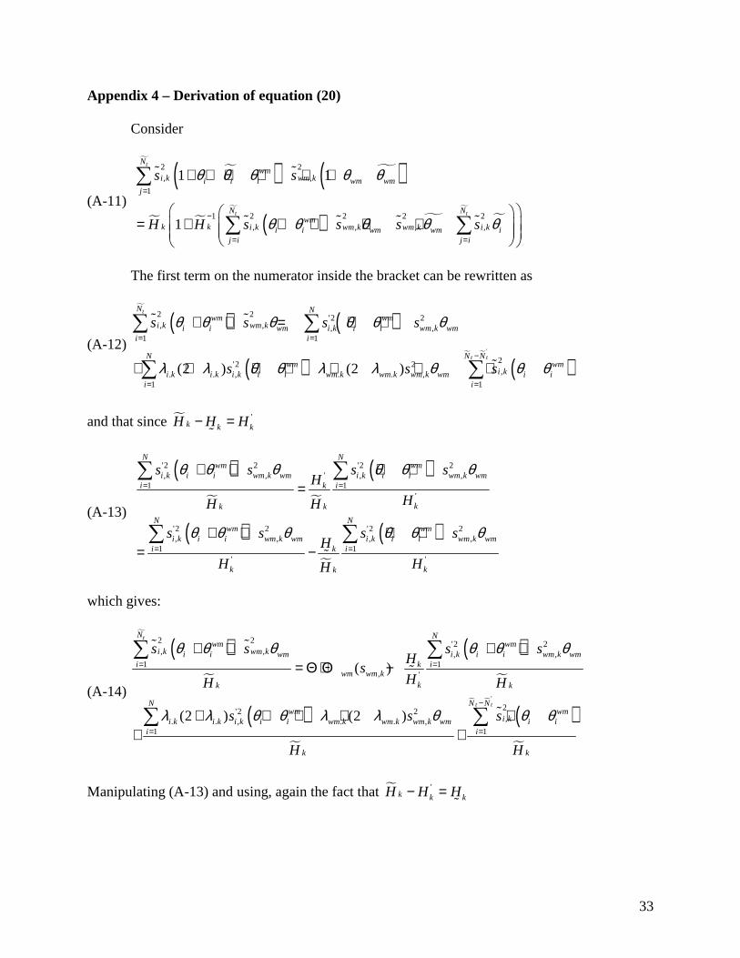
Appendix 4 – Derivation of equation (20)

Consider

(A-11)

�( )�

�( )� �

�

( ) �

�

�

2 2, ,

1

1 2 2 2 2, , , ,

1 1

1

t

t t

Nwm

i k wm ki i i wm wmj

N Nwm

k k i k wm k wm k i ki i wm wm ij i j i

s s

H H s s s s

θ θ θ θ θ

θ θ θ θ θ

=

−

= =

+ + + + + +

= + + + + +

∑

∑ ∑

ɶ ɶ

ɶ ɶ ɶ ɶ

The first term on the numerator inside the bracket can be rewritten as

(A-12)

�

( ) ( )

( )� �

( )'

2 2 '2 2, , , ,

1 1

2'2 2,. . , . . ,

1 1

(2 ) (2 )

t

t t

N Nwm wm

i k wm ki i wm i k i i wm k wmi i

N N Nwm wm

i ki k i k i k i i wm k wm k wm k wm i ii i

s s s s

s s s

θ θ θ θ θ θ

λ λ θ θ λ λ θ θ θ

= =

−

= =

+ + = + +

+ + + + + + +

∑ ∑

∑ ∑

ɶ ɶ

ɶ

and that since � 'k k kH H H− =ɶ

(A-13)

( )� �

( )

( )�

( )

'2 2 '2 2', , , ,

1 1'

'2 2 '2 2, , , ,

1 1' '

N Nwm wm

i k i i wm k wm i k i i wm k wmi k i

kk k

N Nwm wm

i k i i wm k wm i k i i wm k wmi k i

k kk

s s s sH

HH H

s s s sH

H HH

θ θ θ θ θ θ

θ θ θ θ θ θ

= =

= =

+ + + +=

+ + + += −

∑ ∑

∑ ∑ɶ

which gives:

(A-14)

�

( )�

( )�

( )�

� �

( )�

'

2 2 '2 2, , , ,

1 1, '

2'2 2,. . , . . ,

1 1

( )

(2 ) (2 )

t

t t

N Nwm wm

i k wm ki i wm i k i i wm k wmi k i

wm wm kkk k

N N Nwm wm

i ki k i k i k i i wm k wm k wm k wm i ii i

k k

s s s sH

sHH H

s s s

H H

θ θ θ θ θ θ

λ λ θ θ λ λ θ θ θ

= =

−

= =

+ + + += Θ + Θ −

+ + + + ++ +

∑ ∑

∑ ∑

ɶ ɶ

ɶ

ɶ

Manipulating (A-13) and using, again the fact that � 'k k kH H H− =

ɶ

34

�

( ) �

�

�

�

( )�

( )�

� �

( )�

�

�

�

�

'

2 2 2 2, , , ,

,

22'2 '2,,, . . ,

1 1 1'

2,

'

(A 15) ( )

(2 )

t t

tt t

N Nwm

i k wm k wm k i ki i wm wm ij i j i

wm wm k

k

NN N N Nwm wm wm

i ki k ii k i i i k i k i k i i i ij ik i i i

k k k k k

wm k wmk

k k

s s s s

sH

ss s sH

H H H H H

sH

H H

θ θ θ θ θ

θθ θ λ λ θ θ θ θ

θ λ

= =

−

== = =

+ + + +− = Θ + Θ

+ + + +− + + +

− +

∑ ∑

∑∑ ∑ ∑

ɶ ɶ ɶ ɶ

ɶɶ

ɶ

ɶ�

�

�

22,. . ,(2 ) wm kwm k wm k wm k wm wm

k k

s s

H H

λ θ θ++ɶ

Which reorganizing gives:

�

( ) �

�

�

�

( )�

� �

( )�

�

�

� �

�

�

'

2 2 2 2, , , ,

,

22'2, 2, 2. . ,

,. . ,1 1

'2,

(A-16) ( )

(2 )(2 )

t t

tt t

N Nwm

i k wm k wm k i ki i wm wm ij i j i

wm wm k

k

NN N Nwm wm

i ki k ii k i k i k i i i iwm kj i wm k wm k wm k wm wmi i

k k k k k

i ki

s s s s

sH

ss ss s

H H H H H

s

θ θ θ θ θ

θλ λ θ θ θ θ λ λ θ θ

= =

−

== =

+ + + += Θ + Θ

+ + + ++ + + + +

+

∑ ∑

∑∑ ∑

ɶ ɶ ɶ ɶ

ɶɶɶ

( )�

( )�

'22 2,

, ,1 1' '

N Nwm wm

i i i k i iwm k wm wm k wmi

k kk k

ss s

H HH H

θ θ θ θ θ θ= =

+ +− + −

∑ ∑

And since

(A-17)

( )�

( )�

� �

( )�

�

( )�

� � �

'

2 2'2 '2, ,. . , ,

1 1 1 1

22 2,. . , ,

(2 )

(2 )

t tN N N N Nwm wm wm wm

i k i ki k i k i k i i i k i i i i i ii i i i

k k k k

wm kwm k wm k wm k wm wm k wm wm

k k k

s s s s

H H H H

s s s

H H H

λ λ θ θ θ θ θ θ θ θ

λ λ θ θ θ

−

= = = =

+ + + + ++ + =

++ =

∑ ∑ ∑ ∑ɶ ɶ

ɶ

One obtains

�

( ) �

�

�

�

�

( )�

�

�

( ) �( )�

2 2 2 2, , , ,

2 2'2 2

, , 2, ,1 ,1

, ' '

(A 18)

( ) ;

t t

t t

N Nwm

i k wm k wm k i ki i wm wm ij i j i

k

N N Nwm wm

i k i ki i i i k i i wm k wm wmi j i wm k wmiwm wm k

k kk k

s s s s

H

s s s s ss

H HH H

θ θ θ θ θ

θ θ θ θ θ θ θ θ

= =

= = =

+ + + +− =

+ + + +Θ + Θ + − + −

∑ ∑

∑ ∑ ∑

ɶ ɶ ɶ ɶ

ɶ ɶɶ

35

From which, defining �

�

( )�

�

�

( )2 2'2

, , ,1' 1

, , '( ; )

t tN N Nwm wm

i k i ki i i i k i ii j i i

i k i kkk

s s ss

HH

θ θ θ θ θλ = = =

+ + +Θ = −

∑ ∑ ∑ɶ ɶ

and ��( )

�

22,

,, , '

( ; )wm k wm wm wm k wm

wm wm k wm kkk

s ss

HH

θ θ θλ

+Θ = −

ɶ

, gives equation (20).