Embed Size (px)
Citation preview

WAIS 2005; Slide number 1.
Numerical modelling of ocean-ice interactions under Pine
Island Bay’s ice shelf
Tony Payne1
Paul Holland2,3 Adrian Jenkins3
Daniel Feltham2 Andrew Shepherd4
Ian Joughin5
1 Centre for Polar Observation and Modelling, University of Bristol
2 CPOM, University College London 3 British Antarctic Survey, Cambridge
4 CPOM, University of Cambridge 5 University of Washington, USA

WAIS 2005; Slide number 2.
Aim• use two-dimensional
model of density currents
• derives from work on study Svalbard density currents (Jungclaus and others JGR 1995)
• sub-shelf physics of Jenkins (JGR 1991) incorporated
• apply to Pine Island using idealised geometry and realistic forcing
• conduct perturbation experiments to assess effect of recent oceanographic changes
500 km

WAIS 2005; Slide number 3.
Model description• vertically integrated, time
dependent
• mass balance gives plume depth (D) incorporates
– basal ice melt/freeze (interface heat and salt balances with pressure relationship) and
– entrainment (Pedersen) from ambient ocean
• horizontal momentum balances (U and V) (Coriolis, lateral and surface drag, buoyancy etc included)
• temperature (T) and salinity (S) transport with lateral mixing
• linearized equation of state for density
• run to equilibrium in ~ 20 days
ice
plume
ambient
melt/freeze
entrainment
D
T,S,U,VT,S,U,V

WAIS 2005; Slide number 4.
Oceanographic inputs• profiles of ambient
temperature and salinity from Jacobs and others (GRL 1996) -1.9
1.0600 m
33.8
34.7

WAIS 2005; Slide number 5.
Glaciological inputs• profile of ice-shelf base
van der Veen solution tuned to give observed thickness at grounding and shelf front
• laterally constant
• temperature gradient in basal ice (constant at 0.01 C m-1)
• subglacial meltwater outflow (estimated at 3 km3 yr-1) over ice stream width (~0.1 m)
• impermeable lateral boundaries
0 10 20 30 40 50 60 70
-1000
-800
-600
-400
-200
0
Distance from grounding line (km)
Ele
vati
on
(m
)
90 km
70 km
40 km

WAIS 2005; Slide number 6.
Standard results: evolution after 20 days
Velocity and plume depth
(m)
Max. velocity 0.45 m/s.
Grid spacing 500 m (here shown every
2.5 km)
0 10 20 30 40 50 60 70 80 900
10
20
30
40
50
60
70
1
5
10
20
50
5
1
10

WAIS 2005; Slide number 7.
Standard results: evolution after 20 days
Melt rate (m/yr) and
plume depth (m)
Grid spacing 500 m (here shown every
2.5 km)
0
10
20
30
40
50
60
70
80
90
0
10
20
30
40
50
60
70
0
20
40
60
80
0
10
20
30
40
50
60
70

WAIS 2005; Slide number 8.
Standard results: summary
Melt rate m yr-1
Mean modelMaximum model
2572
Jacobs and others (GRL 1996)Oceanographic data
mean 10-12
Rignot and Jacobs (Science 2002)Ice budget
meanmaximum
20-2840-60

WAIS 2005; Slide number 9.
Oceanographic change• Robertson and others (Deep Sea Res.
2002) and Jacobs and others (Science 2002) observations for eastern Ross Sea
• suggest warming ~0.3 C and freshening 0.3 ‰ over last 40 years at 200-400 m
• assume true for Amundsen Sea and apply uniformly with depth

WAIS 2005; Slide number 10.
Perturbation experiment – melt rate as a function of temperature and salinity anomalies
Shepherd and others (GRL 2004) estimate thinning rates from ERS altimetry for Pine Island 3.4 to 4.4 m yr-1
this is to the high end of what we estimate here
WAIS 2005; Slide number 11.
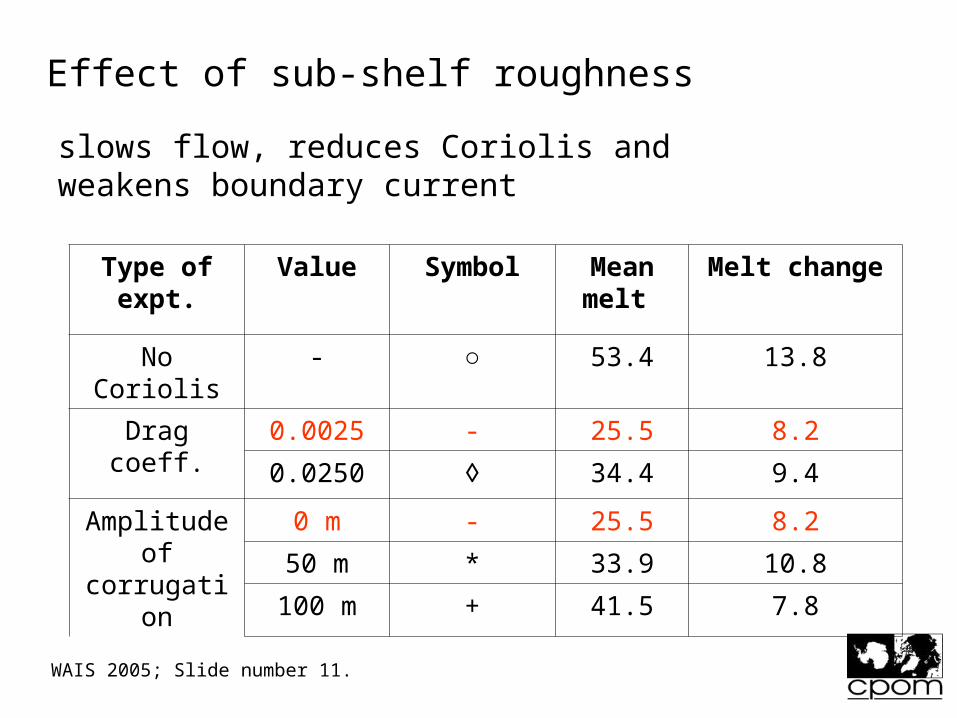
Effect of sub-shelf roughness
slows flow, reduces Coriolis and weakens boundary current
Type of expt.
Value Symbol Mean melt
Melt change
No Coriolis - ○ 53.4 13.8
Drag coeff. 0.0025 - 25.5 8.2
0.0250 ◊ 34.4 9.4
Amplitude of
corrugation
0 m - 25.5 8.2
50 m * 33.9 10.8
100 m + 41.5 7.8

WAIS 2005; Slide number 12.
Summary• melt rates concentrated at GL (warm water at
depth) and in boundary current (high velocity)
• perturbation experiments forced using observed changes in oceans reproduce estimated thinning rates
• sensitivity estimated as 16-20 m yr-1C-1 compared to Rignot and Jacobs [Science 2002] sensitivity 10 m yr-1C-1
• results suggest warming of ~0.5 C would be sufficient to explain thinning

WAIS 2005; Slide number 13.
OCCAM global ocean circulation model
0.25 global grid, 66 levels
spun up by restoring to Levitus 1994 data for 4 yrs
forced with NCEP 6-hourly data 1985 to 2003

WAIS 2005; Slide number 14.
CDW?
Max. water temperature as a function of latitude and date

WAIS 2005; Slide number 15.
Movie of mean water temperature between 400 and 1000m depth