Embed Size (px)
Citation preview

Wages, productivity, and market power∗
Oleksandr Shepotylo†, Philip Ushchev ‡, and Volodymyr Vakhitov§
November 5, 2014
Abstract
We explore relationships between wages, productivity and market power within a frame-
work that captures labor market rigidities, �rm heterogeneity, and variable markups. Pro-
ductivity is only one of the factors that potentially can explain variation of wages within an
industry. Another important determinant of wages can be the �rm's market power. More
precisely, the outcome of the bargaining game between a �rm and its workers depends cru-
cially on the demand side characteristics. Hence, �rm's markup also may serve as a good
explanatory variable for the wage rate set by the �rm. We provide a micro foundation for this
channel of wage determination.
We test our predictions using Ukrainian �rm-level data. An increase in productivity weakly
increases an average wage within a �rm, but the e�ect is small and not robust. The elasticity of
wage with respect to labor productivity is 0.064 in the baseline speci�cation, but the coe�cient
is not statistically signi�cant. An increase in the markup also results in an increase in the
average wage. The e�ect is almost three times higher, statistically signi�cant, and is robust
to various model speci�cations. The positive sign of the markup coe�cient indicates that the
elasticity of aggregate demand is decreasing function of output. Based on the industry-level
analysis, we �nd evidence supporting the bell-shaped relationship between the coe�cient of
variation of wages and the share of exporting �rms in the industry.
Keywords: Wage bargaining; wage inequality; heterogeneous �rms; productivity; variable
markups; international trade; monopolistic competition
JEL Classi�cation: D43, F12, J31
∗We thank C. d'Aspremont, K. Behrens, R. Dos Santos, D. Levando, M. Parenti and J.-F. Thisse for valuablesuggestions. The �nancial support from the Government of the Russian Federation under the grant 11.G34.31.0059is acknowledged.†University of Bradford, [email protected]‡Higher School of Economics, [email protected]§Kyiv School of Economics and Kyiv Economic Institute, [email protected]
1

1 Introduction
Rising wage inequality across and within countries over the last 20 years, which according to
OECD (2012) was the main contributor to the rising household income inequality in both rich
and poor countries, is often linked to globalization. According to Goldberg and Pavcnik (2007),
trade liberalization in Chile in 70's, in Mexico in 80's, in Argentina, Colombia, and India in 90's
came along with the increasing wage inequality. The traditional Heckscher-Ohlin model fails to
explain an increasing wage gap between skilled and unskilled labor that occurred both in rich and
poor countries over the last two decades. In addition, it cannot account for a large variation in
wages within a narrowly de�ned industry reported in the literature (Dunne et al., 2004). Recently,
Helpman et al. (2010, hereafter HIR) (and some others authors, including (Egger and Kreickemeier,
2012; Felbermayr et al., 2011; Amiti and Davis, 2012) suggested a new class of models that link
changes in wage inequality to the distributional changes in productivity within an industry. In
their framework, heterogeneous �rms, facing a labor market with search and matching frictions,
in equilibrium pay wages that increase with productivity. Wage inequality within an industry in
these models is driven by technological di�erences acorss �rms.
However, these models are based on identical constant elasticity of substitution (CES) prefer-
ences across consumers, which precludes any e�ect of trade liberalization on �rm's market power.
More precisely, because CES preferences generate an isoelastic market demand, the equilibrium
markups are constant. This prediction does not seem realistic � substantial variation of markups
across �rms is well-documented (De Loecker and Warzynski, 2012). Moreover, the variation in
market power across �rms has an important impact on their performance (Syverson, 2004; Fos-
ter et al., 2008). In particular, it can in�uence �rm's wage decision, which is determined in a
bargaining game over the �rm's pro�t.
The link between wages and markups has been extensively studied in recent macroeconomics
literature (i.e. Nakamura and Zerom, 2010). However, to the best of our knowledge, there are no
studies of this link from the international trade perspective. This paper aims to �ll this gap in
the literature. More concretely, we explore relationships of wages, productivity and market power
within a framework that captures labor market rigidities, �rm heterogeneity, and variable markups.
For this purpose, we combine approaches of HIR and Zhelobodko et al. (2012, hereafter ZKPT).
HIR explains variation in wages as a result of exogenous variation in productivity. However,
productivity is only one of the factors that potentially can explain variation in wages. Another
important determinant of wages can be the �rm's markup. To be precise, bargaining game between
workers and the �rm is about splitting the revenue, which depends on the market power. We
provide a micro foundation for this channel, which stems from the fact that the outcome of the
bargaining game crucially depends on the demand side characteristics.
Our main results may be summarized as follows. First, we derive the wage-productivity equa-
tion, which describes the link between �rm-level productivities, markups, and wages. This equation
2

says that more productive �rms charge higher wages. Moreover, �rms with higher market power
charge higher (lower) wages if and only if the aggregate demand elasticity is a decreasing (increas-
ing) function of output.
Second, we estimate the log-linearized version of the wage-productivity equation, focusing
mainly on the sign of the markup coe�cient, because the elasticity of wage with respect to the
markup summarizes all the relevant features of the demand structure of the model.
Third, to cope with endogeneity of markups, we use the result that markups of exporting
�rms depend on trade costs and demand charactristics of importing countries. We also exploit
the regulatory changes in trade policy to generate an exogenous variation in �rms' productivity in
order to solve an omitted variable bias, which arises due to unobserved workers' abilities.
In addition, an increase in productivity leads to an increase in the average wage per worker, but
the result is economically small and not robust. The elasticity of wage with respect to productivity
is 0.064 in the baseline speci�cation. An increase in the markup also results in the increase in the
average wage, but the e�ect is three times higher and is robust to various model speci�cations.
The positive sign of the markup coe�cient indicates that the elasticity of aggregate demand is
decreasing function of output.
Finally, based on the industry-level analysis, we �nd evidence supporting the bell-shaped re-
lationship between the coe�cient of variation of wages and the share of exporting �rms in the
industry. Finally, we propose a method of estimating superelasticity of aggregate demand, which
is di�erent from the one suggested by Nakamura and Zerom (2010).
The rest of the paper proceeds as follows. Section 2 develops a theoretical model and derives
the wage-productivity equation. Section 3 describes the data. Section 4 outlines the identi�cation
strategy. Section 5 presents results. Section 6 concludes.
2 Model
In this section we describe our theoretical framework that combines features of HIR and ZKPT.
As in Helpman et al. (2010), we consider a two-country model with costly trade. Markets are
monpolistically-competitive, which means that each �rm is non-atomic. Firms are heterogeneous
in productivity and workers are heterogeneous in ability. Labor market has two sources of imper-
fections. First, �rms do not directly observe workers' abilities, hence they bear screening costs.
Second, the search process for job candidates is costly. Unlike HIR, we do not impose any paramet-
ric speci�cations of preferences. Instead, in the spirit of ZKPT, we assume non-speci�ed additive
preferences, which implies that �rms face non-isoelastic demands on both home and foreign mar-
kets. In addition, we do not restrict the model to a speci�c parametrization of the distribution of
abilities. Our model is described as follows.
3

2.1 Consumers
Each of the two countries is populated by a unit mass of consumers. Consumers share the same
additive preferences given by
U ≡N
0
u(qi)di+
N∗ˆ
0
u(q∗j )dj (1)
where qi is consumption of domestic variety i and q∗j is consumption of foreign variety j. Each
consumer maximizes (1) subject to the budget constraint
N
0
piqidi+
N∗ˆ
0
p∗jq∗jdj ≤ w (2)
The individual inverse demand for variety i is given by
pi =u′(qi)
λ(3)
where λ is the Lagrange multiplier **of the program (1) � (2),** which shows marginal utility of
income.
It is worth noting that consumers are heterogeneous in income, because workers with di�erent
levels of ability may earn di�erent wages. As a consequence, the values of λ may also vary
across consumers. We denote Λ and Λ∗as the distribution of λ's at home and foreign countries
respectively.
2.2 Firms
Each country accommodates a continuum of �rms. As mentioned, we assume that �rms are
non-atomic, which means that the impact of �rm's behavior on market aggregates is negligible.
**In other words, unlike oligopoly models, here �rms are not involved into strategic interactions.
However, they are involved into weak interactions, which occur through the impact of collective
�rms' behavior on the market aggregates.** Firms are heterogeneous in overall productivity θ
drawn from a distribution Γ(θ), **which is** common for both countries. Each �rm produces at
most one variety, and each variety is produced by at most one �rm. In other words, there are no
scope economies.
Equation (3) implies that the aggregate demand faced by domestic �rm i at the domestic
market is given by
yi = D(pi; Λ) ≡∞
0
(u′)−1
(λpi)dΛ(λ) (4)
4
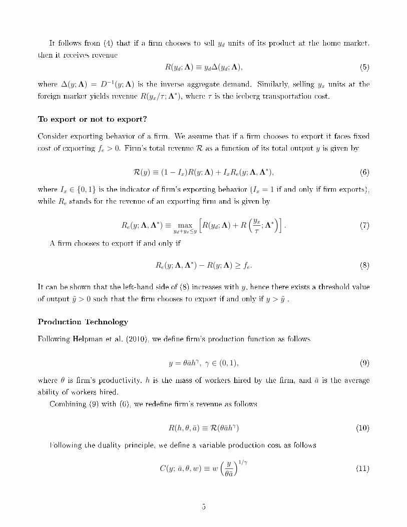
It follows from (4) that if a �rm chooses to sell yd units of its product at the home market,
then it receives revenue
R(yd; Λ) ≡ yd∆(yd; Λ), (5)
where ∆(y; Λ) = D−1(y; Λ) is the inverse aggregate demand. Similarly, selling yx units at the
foreign market yields revenue R(yx/τ ; Λ∗), where τ is the iceberg transportation cost.
To export or not to export?
Consider exporting behavior of a �rm. We assume that if a �rm chooses to export it faces �xed
cost of exporting fe > 0. Firm's total revenue R as a function of its total output y is given by
R(y) ≡ (1− Ix)R(y; Λ) + IxRe(y; Λ,Λ∗), (6)
where Ix ∈ {0, 1} is the indicator of �rm's exporting behavior (Ix = 1 if and only if �rm exports),
while Re stands for the revenue of an exporting �rm and is given by
Re(y; Λ,Λ∗) ≡ maxyd+yx≤y
[R(yd; Λ) +R
(yxτ
; Λ∗)]. (7)
A �rm chooses to export if and only if
Re(y; Λ,Λ∗)−R(y; Λ) ≥ fe. (8)
It can be shown that the left-hand side of (8) increases with y, hence there exists a threshold value
of output y > 0 such that the �rm chooses to export if and only if y > y .
Production Technology
Following Helpman et al. (2010), we de�ne �rm's production function as follows
y = θahγ, γ ∈ (0, 1), (9)
where θ is �rm's productivity, h is the mass of workers hired by the �rm, and a is the average
ability of workers hired.
Combining (9) with (6), we rede�ne �rm's revenue as follows
R(h, θ, a) ≡ R(θahγ) (10)
Following the duality principle, we de�ne a variable production cost as follows
C(y; a, θ, w) ≡ w( yθa
)1/γ
(11)
5

For a non-exporting �rm, the markup is given by
m ≡ p− ∂C/∂yp
For an exporting �rm, the markups are
md ≡pd − ∂C/∂y
pd, mx ≡
px − ∂C/∂ypx
Note that the �rm can charge di�erent markups at home and foreign markets.
2.3 Labor market
A worker is endowed with a speci�c level of ability a drawn from a distribution G(a). Firms do not
observe a, but know G(·). In contrast to Helpman et al. (2010) we do not assume any parametric
speci�cation of G.
Each �rm chooses the mass n of workers to be interviewed. Search requires a constant cost
b > 0 for an additional worker to be interviewed. Even though a is not observable, the �rm can
set up a screening process that allows to �nd out whether the worker's ability exceeds a screening
threshold ac chosen by the �rm. The �rm bears screening costs S(ac), which are assumed to satisfy
S ′(ac) > 0, S ′′(ac) ≥ 0, and hires a worker if and only if a > ac. Thus, the mass of hired workers
is determined as h = [1−G(ac)]n, while the average ability of workers within the �rm is given by
a =
ˆ ∞ac
adG(a)
1−G(ac)(12)
In other words, average ability within the �rm is the mean of distribution G, truncated at the level
ac.
Wage bargaining process
We now come to the wage determination process. We assume that, given n and ac (hence h and a),
each �rm is involved in a bargaining game with its potential workers. To describe the bargaining
process, we use the approach proposed by (Stole and Zwiebel, 1996). This approach takes into
account that a �rm internalizes potential gains or losses from re-negotiation, which arise when the
number of workers changes (e.g. if an applicant leaves without achieving an agreement on the
wage). As a consequence, it must be that, given θ and a, the negotiated wage wneg(h, θ, a) satis�es
the following equation:
∂R
∂h= w +
∂(wh)
∂hfor all h > 0. (13)
Equation (13) brings together two ideas. First, the wage-setting game results in �rm's marginal
6

bene�ts ∂R/∂h of hiring an extra worker being equal to marginal hiring costs. Second, �rms
internalize re-negotiation e�ects captured by the second term of the right-hand side of (13): in
addition to the wage w paid to an extra worker, marginal hiring cost includes a change in total
wage bill ∂(wh)/h.
Solving (13), we �nd that the total wage bill is given by
hwneg(h, θ, a) = R(h, θ, a)− 1
h
hˆ
0
R(ξ, θ, a)dξ (14)
Claim. The negotiated wage decreases with h if and only if R(h, θ, a) is concave in h.
See Appendix 1 for deriving (14), as well as for the proof of the Claim.
Denote through β(h, θ, a) the bargaining power of �rm θ, measured as the share of revenue
attributed to �rm θ:
β(h, θ, a) ≡ R(h, θ, a)− hwneg(h, θ, a)
R(h, θ, a). (15)
It is worth noting that, unlike in HIR, �rms' bargaining power is no longer constant, it now
varies with h. Indeed, combining (14) with (15), we obtain
β(h) =
´ h0R(ξ, θ, a)dξ
hR(h, θ, a). (16)
Do larger (in terms of h) �rms always enjoy higher bargaining power in the wage setting process
than the smaller ones? We show in Appendix 1 that the elasticity of β with respect to h is given
by
Eh(β) ≡ ∂β
∂h
h
β=
´ h0R(ξ, θ, a) [Eξ(R)− Eh(R)] dξ´ h
0R(ξ, θ, a)dξ
. (17)
Inspecting (17), we come to a proposition.
Proposition 1. Given θ and a, �rms' bargaining power increases (decreases) with the number
of workers if the elasticity of revenue Eh(R) is a decreasing (increasing) function of h.
Recall that
R(h, θ, a) = θahγ∆(θahγ).
Hence, we have Eh(R) = γ [1− η(y)], which implies the following corollary of Proposition 1.
Corollary. Given θ and a, �rms' bargaining power increases (decreases) with the number of
workers if the inverse demand elasticity η(y) is an increasing (decreasing) function of y.
This result clearly shows that it is the demand side which is crucial for the wage bargaining
outcome.
7

Figure 1: Amount of labor vs bargaining power.
As shown by Figure 1, the relationship between the amount of labor and �rm's bargaining
power is essentially positive. This provides indirect evidence that assuming CES utility may be
too restrictive for theoretical predictions of HIR to data.
2.4 Pro�t maximization
Each �rm chooses how many workers to interview n, how many workers to hire h, screening
threshold ac, and the decision whether to export Ix in order to maximize pro�t
π = R(h, θ, a)− wh− bn− S(ac)− fd − feIx
Using h = [1−G(ac)]n, (12), as well as (13), the �rm's problem may be reformulated as follows
maxac,h,Ix
1
h
hˆ
0
R(ξ, θ, a)dξ − bh
1−G(ac)− S(ac)− fd − feIx
(18)
8

The �rst order condition ∂π/∂h = 0 yields
w = b/(1−G(ac)) (19)
The intuition behind (19) is as follows. According to Stole and Zweibel bargaining procedure,
the �rm's marginal bene�t of having one more worker is equal to w. On the other hand, given the
screening threshold ac, b/(1−G(ac)) is a marginal replacement cost. Thus, (19) states that at the
optimal level of employment, the �rm equates the marginal cost and marginal bene�t of hiring a
worker. It also implies that the pro�t maximizing level of the total wage bill is equal to the total
search cost. Another important message sent by (19) is that �rms making tougher requirements
typically pay higher wages � there is an increasing relationship between w and ac, independent
from the other endogenous variables. As a consequence, wage is uniquely pinned down by the
screening threshold, regardless of the other decisions of the �rm on production and exporting.
Setting ∂π/∂ac = 0, we obtain
g(ac)
1−G(ac)
[(1− ac
a
) 1
γ− 1
]w
S ′(ac)=
(θ
y
)1/γ
(20)
Equation (12) de�nes a one-to-one relationship between ac and a. Combining this with (19), we
may restate (20) as follows
θ
y= φ(w) (21)
where
φ(w) =
[g(ac(w))
1−G(ac(w))
((1− ac(w)
a(ac(w))
)1
γ− 1
)w
S ′(ac(w))
]γIt can be shown that φ′(w) > 0 when (i) G is Pareto, while S is power function or (ii) G
is exponential, while S is linear. Under these circumstances, output and wages are negatively
correlated for �rms with the same productivity level. Combining (21) with production function
equation (9), this can be interpreted as a downward-sloping demand for labor
h∗(w) =
(1
a(ac(w))φ(w)
)1/γ
(22)
It is worth-noting that this demand is the same for all �rms, because it is independent of θ.
However, this property depends crucially on the power speci�cation of production function.
2.5 Wage-productivity equation
Equation (21) can be rewritten as follows
lnw = Ψ(ln θ − ln y) (23)
9

Furthermore, it can be shown that the pro�t-maximizing markups for a non-exporting �rm
satisfy the standard monopoly pricing rule
m = η(y), (24)
where η(y) is the inverse aggregate demand elasticity :
η(y) ≡ −∂∆
∂y
y
∆(25)
Using (24) and a linear Taylor approximation of (23), we obtain
lnw ≈ ln w + δθ(ln θ − ln θ) + δm(lnm− ln m) (26)
where
δθ = Ψ′(ln θ − ln y), δm = −δθη(y)
yη′(y). (27)
Notice that δmδθ
= − yη′(y)η(y)
is the superelasticity of inverse aggregate demand as de�ned by Klenow
and Willis (2006). Thus, our model suggests a natural estimator of superelasticity, di�erent from
the one used by Nakamura and Zerom (2010).
Equation (26) can be estimated using a log-linear regression. Moreover, it follows immediately
from (27) that (i) δθ > 0, (ii) δm > 0 if and only if η(y) is an increasing function of y, (iii)
δθ + δm = 0 if and only if yη′(y)η(y)
= 1. The last condition holds regardless of a speci�c value of y
if and only if η is linear in y, which is equivalent to ∆(y) = A exp(−κy). In other words, inverse
aggregate demand varies with y as if it was generated by a representative consumer with CARA
utility: u(q) = 1− exp(−κq). (see Behrens and Murata (2007) for details).
For exporting �rms domestic and exporting markups are given by=
md = η(yd), mx = η(yxτ
). (28)
Linearizing (23), we obtain
lnw ≈ c+ δθ ln θ + δM lnm (29)
where
m = mα
α+β
d mτ βα+β
x (30)
is a composite markup and
δθ = Ψ′(ln θ − ln y), δM = −δθ(α + β) (31)
α =η(yd)
ydη′(yd)
ydy, β =
η(yx)
yxη′(yx)
yxy
10

It is clear that markups are endogenously determined within the model. First, they depend on
exogenous trade costs τ . Second, note that aggregate demand elasticity η also depends on Λ and
Λ∗. This justi�es including observable trade costs measures and market aggregates statistics, such
as aggregate demand and income inequality, as instruments that generate exogenous variability in
the markups across �rms.
3 Data
To explore links between wages, productivity, and markups we use Ukrainian �rm-level data in
2001-2007. The data are from the State Statistics Service of Ukraine (UKRSTAT). We restrict
our sample to manufacturing �rms (NACE Revision1.1 Section �D�) with 20 or more workers.1 We
de�ne manufacturing industries as NACE Revision1.1 divisions 15-37. We combine industries 15
(Manufacture of food products and beverages) and 16 (Manufacture of tobacco products) into one
industry (15+16) due to small number of �rms in industry 16. This gives us 22 manufacturing
industry.
As the measure of output, Y , we use �Net sales after indirect taxes� from the Financial Results
Statement. The Balance Sheet Statement is the source of the capital measure, K, for which we use
�End-of-year value of tangible assets.� Employment (L), material costs (M), and investment (I)
come from the Enterprise Performance Statement. Employment is measured as the �Year-averaged
number of enlisted employees�. For investment, we use �Investments in tangible assets.�
We exclude observations with zero or negative output, capital stock or employment. Based on
the �les accompanying the Enterprise Performance Statement and the Balance Sheet Statement,
we create a comprehensive pro�le for every �rm, which includes the territory code and the four-
digit sub-industry code, fully compatible with NACE classi�cation. Output measure is de�ated
by industry price de�ators. Capital, investments and material costs are de�ated by PPI. Annual
FDI statements let us identify �rms with foreign ownership, de�ned as ownership of more than 10
percent of the company by a foreigner. We use annual customs data to de�ne an export-to-sales
share and importing status of a �rm. Also, we generate entry and exit indicator variables, marking
the entry as the �rst year when a �rm appeared in the sample, and the exit as the last year when
a �rm appeared in the sample. Periods between exit and entry were marked as zeros, even though
a �rm could disappear from the sample for some years. In year 2007, the value of the exit variable
is assumed to be zero, to be consistent with Olley and Pakes (1996). Similarly, the entry variable
is assumed to be zero for all �rms in 2001.
The descriptive statistics for the full and restricted samples are presented in Table 1.
The full dataset contains over 18,000 manufacturing �rms with average employment of 208
employees. However, only approximately 10,000 manufacturing �rms (in 2007, this number fell to
1Our results for all manufacturing �rms do not di�er neither in statistical signi�cance nor in size of the coe�cientpoint estimates. Results are available upon request.
11

2,700 �rms due to a change in the sample composition), that we call a restricted sample, report the
Annual Sectoral Expenditures Statement with detailed �rm's expenditures on purchases from 22
manufacturing industries and 15 service sub-sectors. These data are essential for our identi�cation
strategy, allowing us to construct instruments for productivity and markups. Average employment
of reporting manufacturing �rms in the restricted sample is 334 workers. These �rms produced
over 75% of the annual manufacturing output of Ukraine (which fell to 60% in 2007). were used to
construct �rm-speci�c indices of services liberalization for the restricted sample, which were used
as instruments for productivity.
4 Empirical strategy
The empirical counterpart of equation (29) is
lnwit = α + δθ ln θit + δm lnmit + δexp × exportit+ (32)
δθexp × exportit ln θit +Xitγ +Dsts+Drr + εit
where wit is �rm i′s average wage at time t. θit is �rm i′s measured productivity at time t. mit is
�rm i′s average markup, exportit is the export-to-sales share. Dst are industry-year �xed e�ects,
and Dr are region �xed e�ects. X represents a vector of additional controls.
Based on the theory developed inSection 2, we expect δθ > 0, which re�ects the well-documented
stylized fact that more productive �rms pay higher wages (Amiti and Davis, 2012). However, the
behavior of δm is more versatile. It is positive (negative) if and only if inverse demand elasticity is
a decreasing (increasing) function of y, i.e. when larger �rms charge lower (higher) markups.
4.1 Productivity measures
In the empirical analysis we use two measures of productivity � labor productivity and total factor
productivity (TFP). Labor productivity is constructed as the value added de�ated by the industry
price de�ator divided by the number of workers. To recover the TFP measure, we estimate the
production function for each manufacturing industry (2-digit NACE classi�cation) by the Olley-
Pakes procedure (Olley and Pakes, 1996), controlling for the sub-industry-speci�c demand and price
shocks as suggested by De Loecker (2011). We identify the demand and price shocks by exploiting
variation in sub-industry (4-digit NACE classi�cation) output at time t and by controlling for
sub-industry and time �xed e�ects. As a new result, we demonstrate the De Loecker methodology
is valid under non-CES preferences.
12

Variable Observations Mean Std. deviationA. Summary statistics. Full sample
wit per worker, thsd UAH 2001 74989 4.613 3.653yit, thsd. UAH 2001 74989 15413 143590hit, workers 74989 208.1 1092kit, thsd. UAH 2001 74264 5333 39610matit, thsd. UAH 2001 74263 9877 116846Iit, thsd. UAH 2001 49327 1797 18318ln(θi,t) 69219 1.094 1.401vait/hit 74263 20 43.77Importeri,t 74989 0.2534 0.435Export to salesi,t 74989 .1039 .2449Foreigni,t 74989 0.0766 0.266Exiti,t 74989 0.02772 0.1642Entryi,t 74989 0.05119 0.2204Urbani 74989 0.7115 0.4531Privatei,t 74989 0.9274 0.2594Single plantit 74989 0.9573 0.2022
B. Summary statistics. Restricted sample
wit per worker, thsd UAH 2001 40562 5.074 3.979yit, thsd. UAH 2001 40562 26066 192037hit, workers 40562 333.8 1451kit, thsd. UAH 2001 40562 9099 52871matit, thsd. UAH 2001 40562 16909 156834Iit, thsd. UAH 2001 32377 2486 22339ln(θi,t) 40562 1.073 1.357vait/hit 40562 23.52 52.29Importeri,t 40562 0.3452 0.4754Export to salesi,t 40562 .1342 .2651Foreigni,t 40562 0.096 0.2946Exiti,t 40562 0.01985 0.1395Entryi,t 40562 0.01723 0.1301Urbani 40562 0.6874 0.4636Privatei,t 40562 0.8958 0.3055Single plantit 40562 0.9292 0.2564Input tari�it 40562 4.918 3.151Serv. Libit (EBRD) 40562 0.3506 0.5376
Table 1: Descriptive statistics
13

TFP estimation
Consider a production technology of a single-product �rm i at time t described by production
function
yit = hαhit kαkit mat
αmatit exp(ωit + uit), (33)
where yit units of output are produced using hit units of labor, kit units of capital, and matit
units of material and services inputs. ωit is �rm-speci�c productivity that includes both technical
e�ciency and workers' average ability, unobservable by an econometrician, but known to the �rm
before it chooses variable input hit. uit is an idiosyncratic shock to production that also captures
measurement error introduced due to unobservable input and output prices.
Output yit is not observed, because we do not know �rm-speci�c prices pit. Observable sales,
Rit = pityit, re�ect di�erences in physical quantities as well as variation in markups across �rms
within the same industry. Therefore, use of Rit as the dependent variable in estimation of pro-
duction function parameters, without controlling for prices, determined among other things by
market structure and demand shocks, would bias estimates of the production function if prices are
correlated with inputs.
To deal with this issue, we introduce the following inverse demand system:
pit =u′s(yit)
λstexp(ξit), i ∈ Is (34)
where Is is the set of �rms in industry s, yit is the output of �rm i ∈ Is in the period t, us(·) is theutility function speci�c for industry s, ξit is a random shock in demand, while λst is the Lagrange
multiplier of the consumer's problem.
Taking logs and rearranging (34) yields
ln yitu′s(Yit)− ln yitpit = lnλst + ξit.
Setting Rit ≡ Yitpit, we get
lnRit = ln yitu′s(yit)− lnλst + ξit (35)
Let Yst be total consumer's expenditure on products in industry s at time t. Then, using (34)
and the consumer's budget constraint∑
j∈Is pityit = Yst, we implicitly de�ne λst = Λ(Yst,pst) by
Yst =∑j∈Is
pjt (u′s)−1
(λstpjt). (36)
To estimate (35), we log-linearize it in the neighbourhood of the average point(ps, Ys
), where
14

ps ≡
(1
|Is|∑j∈Is
pjt
)· 1, Ys ≡
1
|Is|∑j∈Is
Yjt.
Doing so, we obtain
lnRit ≈ const + (1 + ru(Y )) ln yit −∂ ln Λ
∂ lnYst
∣∣∣∣avg
lnYst −∑j∈Is
∂ ln Λ
∂ ln pjt
∣∣∣∣avg
ln pjt + ξit. (37)
Here and in what follows (·)|avg means that the elasticities are evaluated at(ps, Ys
).
Thus, we need to know the elasticities of Λ with respect to Yst and pit. Implicitly di�erentiating
(36), we obtain
∂ ln Λ
∂ lnYst= −
[∑j∈Is
θjtηjt
]−1
,∂ ln Λ
∂ ln pit= −1− ηit
ηit
(∑j∈Is
θjtθit
1
ηjt
)−1
, (38)
where ηjt ≡ −yjtu′′(yjt)/u′(yjt) is the inverse demand elasticity evaluated at yjt, while θjt ≡ pjtyjtYst
is the share of total expenditure spent on product j at time t. At the average point, i.e. when
pjt = p, yjt = Ys, formulas (38) boil down to
∂ ln Λ
∂ lnYst
∣∣∣∣avg
= −η(Ys),∂ ln Λ
∂ ln pit
∣∣∣∣avg
= −1− η(Ys)
|Is|. (39)
Hence, the log-linear Taylor approximation of Λ(Yst,p) in a small neighbourhood of the average
point is given by
ln Λ(Yst,p) ≈ const− η(Ys) lnYst − [1− η(Ys)]1
|Is|∑j∈Is
ln pjt. (40)
Plugging (40) into (37), we obtain
ln(Rit/Pst) ≈ const + (1 + η(Ys)) ln yit − η(Ys) ln(Yst/Pst) + ξit, (41)
where Pst is the price index de�ned as a simple geometric average of prices in industry s:
Pst ≡
(∏j∈Is
pjt
) 1|Is|
.
Finally, combining (41) with the production function (33), we come to
rit = βh lnhit + βk ln kit + βm lnmatit + βs lnYst + ωit + ξit + uit, (42)
where rit = ln(Rit/Pst) is log of revenue de�ated by corresponding industry (NACE 2 digit ) price
de�ator. βf = σs+1σs
αf , where f = {h, k,mat}. The elasticity of substitution in industry s can be
15

retrieved as σs = 1/η(Ys) = −1/βs. Finally, ωit = σs+1σs
ωit, ξit = − 1σsξit, and uit = σs+1
σsuit are error
terms. In what follows, we suppress the sector index for clarity of presentation.
We estimate equation (42) separately, for each manufacturing industry, using the Olley-Pakes
methodology (Olley and Pakes, 1996) and accounting for demand shocks as outlined above. Instead
of using total industry output, we use more disaggregated sub-industry g output (NACE 4 digit),
ygt, to add more variability to the estimation of σs. We decompose the overall demand shock into
the following components
ξit = ξt + ξg + ξit, (43)
where ξt is industry-speci�c shock common to all �rms at time t, ξg is demand factor a�ecting only
�rms producing in sub-industry g, and ξit is an idiosyncratic shock. Plugging in (43) in (42), we
obtain the following equation
rit = βh lnhit + βk ln kit + βm lnmatit + βs lnYgt + δtDt + δgDg + ωit + εit (44)
where Dt is a a year �xed e�ect and Dg is a sub-industry �xed-e�ect. εit = ξit + uit is the error
term which is not correlated with inputs and productivity.
Results of the estimation are presented in Table 2. Total factor productivity net of price and
demand e�ects is recovered as
ln θit = (rit − βh lnhit − βk ln kit − βm lnmatit − βs lnYgt)σs
σs + 1. (45)
4.2 Markups
We recover �rm-speci�c markups following a procedure developed by De Loecker and Warzynski
(2012). The markups are computed as
mit =pit
∂C/∂y=
βlωitHit/pitYit
. (46)
The procedure does not impose any assumptions on the demand side and market structure and
allows a general from of the continuous and twice-di�erentiable production function.
To be consistent with our theoretical model, we rede�ne markups as follows
mit = 1− 1/mit.
Since we do not have information on how labor is used in production for di�erent markets, this
measure re�ects an average markup and do not vary with market-destination.
We obsere that markups increase with �rm size, measured by sales. In our speci�cations it means
16

Industry ln(k) ln(h) ln(mat) ln(Y ) Firms Nβk αk βh αh βmat αmat βs
15+16 0.045*** 0.048 0.285*** 0.303 0.647*** 0.687 0.058* 7133 24720(0.012) *** (0.012) *** (0.011) *** (0.027)
17 -0.007 -0.007 0.356*** 0.364 0.565*** 0.577 0.022 787 2118(0.028) (0.040) *** (0.019) *** (0.044)
18 0.106** 0.112 0.487*** 0.513 0.454*** 0.478 0.051 1462 4458(0.039) ** (0.025) *** (0.012) *** (0.052)
19 0.148* 0.238 0.383*** 0.616 0.550*** 0.884 0.378* 411 1302(0.069) (0.034) *** (0.022) *** (0.179)
20 0.081*** 0.087 0.297*** 0.320 0.619*** 0.667 0.072 2696 6438(0.021) *** (0.022) *** (0.012) *** (0.047)
21 0.040 0.044 0.186*** 0.205 0.588*** 0.649 0.095 611 1990(0.052) (0.034) *** (0.033) *** (0.083)
22 0.098*** 0.092 0.454*** 0.428 0.453*** 0.427 -0.061* 4407 12520(0.020) *** (0.021) *** (0.010) *** (0.028)
23 -0.124* -0.124 0.218* 0.218 0.492*** 0.491 -0.002 213 634(0.060) * (0.089) * (0.054) *** (0.107)
24 0.133*** 0.145 0.259*** 0.283 0.563*** 0.616 0.086* 1539 4998(0.034) *** (0.030) *** (0.024) *** (0.039)
25 0.094*** 0.103 0.282*** 0.307 0.590*** 0.643 0.083 1944 5867(0.027) *** (0.018) *** (0.015) *** (0.043)
26 0.047 0.050 0.285*** 0.303 0.628*** 0.668 0.059 2874 8993(0.034) (0.022) *** (0.017) *** (0.032)
27 0.034 0.040 0.213*** 0.252 0.636*** 0.753 0.155*** 656 2148(0.041) (0.035) *** (0.031) *** (0.033)
28 0.092*** 0.098 0.303*** 0.324 0.575*** 0.614 0.064 3199 8324(0.018) *** (0.018) *** (0.016) *** (0.037)
29 0.080*** 0.082 0.406*** 0.420 0.442*** 0.457 0.033 4477 13536(0.010) *** (0.014) *** (0.010) *** (0.028)
30 0.221** 0.150 0.691*** 0.468 0.341*** 0.231 -0.477 495 1100(0.076) * (0.061) *** (0.026) *** (0.277)
31 0.097** 0.103 0.326*** 0.348 0.456*** 0.487 0.065 1750 5265(0.033) ** (0.021) *** (0.015) *** (0.047)
32 0.150* 0.155 0.328*** 0.340 0.414*** 0.429 0.035 671 1850(0.067) * (0.046) *** (0.026) *** (0.130)
33 0.065 0.064 0.418*** 0.415 0.431*** 0.428 -0.006 1097 3256(0.039) (0.028) *** (0.017) *** (0.077)
34 0.150* 0.167 0.234*** 0.261 0.540*** 0.601 0.102* 422 1297(0.071) * (0.053) *** (0.052) *** (0.051)
35 -0.030 -0.042 0.442*** 0.605 0.406*** 0.556 0.270*** 755 2485(0.033) (0.044) *** (0.027) *** (0.064)
36 0.085** 0.090 0.345*** 0.362 0.578*** 0.607 0.048 2035 5689(0.027) ** (0.025) *** (0.017) *** (0.036)
37 0.085 0.123 0.628*** 0.914 0.280*** 0.408 0.313* 869 2264(0.068) (0.059) *** (0.027) *** (0.150)
Notes: * p<0.05, ** p<0.01, *** p<0.001. Bootstrap standard errors are presented in parentheses. Table reports point estimates of
revenue function parameters, β and production function paramters α = σsσs+1
β, where σs = −1/βs for Ukrainian manufactruing �rms
for 2001-2007. Each row in the table represents Olley-Pakes estimation of production function for each 2 digit manufacturing industry,
de�ned according to the NACE classi�cation. Each estimation is performed with year and sub-industry dummies, which are not
reported for brevity.
Table 2: Estimation of production function by Olley-Pakes procedure
17

Figure 2: Output vs markups
18

that the inverse elasticity of demand is an increasing function of the �rm size.
4.3 Endogeneity of productivity and markups
Productivity
In the HIR framework, productivity is split into two components � technical e�ciency θit and
average ability of workers, a, which is increasing with the screening intensity. Since we do not have
information on a, our productivity measure includes both components. Unobserved average ability
is positively correlated with both wage and productivity. It means that corr(a, θ) > 0, and leads
to an upward bias in estimation of δθ. Alternatively, in the framework of Egger and Kreickemeier
(2012) and (Amiti and Davis, 2012) based on the fair wage hypothesis (Akerlof and Yellen, 1990),
a wage rate below some level w∗, considered as a fair wage by workers, would lower their level of
e�ort, e, leading to lower productivity. The positive correlation between an unobserved e�ort and
productivity, corr(e, θ) > 0, leads to a positive bias in the OLS estimation of the coe�cient δθ.
To estimate equation (32) consistently, a source of exogenous variation in productivity is needed.
We propose a well-known link from deregulation to productivity as such variation. Recent studies
of services and trade liberalization Amiti and Konings (2007); Arnold et al. (2011); Fernandes
and Paunov (2011); Khandelwal and Topalova (2011) �nd positive e�ect of the liberalization on
productivity of manufacturing �rms. The size of the e�ect varies across �rms because of di�erences
in intensity, with which �rms use liberalized goods and services as inputs.
We use the episode of the Ukrainian trade and services liberalization in 2001-2007, isolated from
other major deregulatory changes and driven by political pressure imposed by Ukraine's trading
partners as a precondition for the Ukrainian WTO accession. Concerning services, the government
developed new laws and amended existing ones that regulated activities of TV and broadcasting,
information agencies, banks and banking activities, insurance, telecommunications, and business
services. It led to di�erentiated but positive e�ect on productivity in the downstream manufactur-
ing �rms (Shepotylo and Vakhitov, 2012). The results indicate that a standard deviation increase
in services liberalization is associated with a 9.2 percent increase in TFP. In parallel with the
services liberalization, the WTO negotiations also led to further liberalization of trade in goods,
which also had a positive e�ect on productivity.
In what follows we descirbe construction of instruments related to endogeneity of productivity
measure. The index of services liberalization is �rm-speci�c, re�ecting the variation in �rm-level
intensity of usage of various services inputs. Similarly to Arnold et al. (2011), but using �rm level
data, the index is computed according to the following formula
serv libit =∑j
ajit × indexjt (47)
19

where ajit is the share of input sourced from the services sub-sector j in the total input for a
�rm i at time t, and indexjt is the measure of liberalization in the service sub-sector j at time
t. The constructed index of services liberalization is further divided by a standard deviation for
normalization. We proxy for indexjt by structural change indicators provided by the European
Bank for Reconstruction and Development (EBRD).2
The second instrument captures the �rm-speci�c measure of trade liberalization. We compute
an index of input tari� liberalization following Amiti and Konings (2007):
input tariffit =∑s
bsit × tariff st (48)
where input tariffit is the �rm-speci�c input tari� measure, bsit is the share of input sourced
from the two-digit NACE industry s in the total input for �rm i at time t, and tariff st is the
trade-weighted average MFN import tari� in industry s at time t.
Markups
The constructed markups are endogenously determined as a function of wages. Since corr(pitθit, εit) <
0, the OLS estimation of (32) would lead to a downward bias in the estimation of the markup
coe�cient. According to equation (28), lnm = αα+β
lnmd+τ βα+β
lnmx, where domestic and foreign
markups depend on domestic and foregin market sizes. Using �rm-level export statistics, we use
construct two instruments to cope with endogeneity of markups. First, we construct a proxy for the
trade costs as the export-weighted average distances τit =∑
jexpijtexpit
ln distij to destination markets,
where expijt is export of �rm i to country j at time t, expit =∑
j expijt is the total export of �rm
i at time t, and distij is distance from Ukraine to country j. Second, we construct a proxy for the
market size as ˆMPit =∑
jexpijtexpit
lnGDPjt, where GDPjtis gross domestic product of country j at
time t. We normalize lnmd as equal to zero, so lnm = 0 for non-exporting �rms.
5 Results
Dynamics of labor productivity, TFP, markups, and wages in 2001-2007 is presented in Table 3.
Over the investigated period, productivity has almost doubled, while dispersion of productivity has
been moderately growing. Markups have also increased, but without noticeable trend in variation.
An increase in the markups during the trade and services liberalization episode is consistent with
�ndings of De Loecker et al. (2012) � during the trade liberalization episode in India, marginal
costs have been reduced by 40 percent, while prices fell only by 16.8 percent, leading to higher
markups.
2EBRD structural change indicators are available at http://www.ebrd.com/pages/research/economics/data/macro.shtml.The mapping from the structural change indicators to sub-sectors of services is explained in the appendix.
20

Year ln vait/hit ln θit lnmit lnwitMean Std. Dev. Mean Std. Dev. Mean Std. Dev. Mean Std. Dev.
A. Full sample2001 1.74 1.375 0.815 1.413 0.757 0.96 0.82 0.7582002 1.951 1.2 0.915 1.409 0.644 0.963 1.045 0.6942003 2.088 1.171 0.995 1.39 0.664 1.003 1.161 0.6642004 2.399 1.129 1.129 1.392 0.772 0.961 1.293 0.6272005 2.578 1.076 1.19 1.359 0.757 0.925 1.48 0.5992006 2.728 1.065 1.264 1.389 0.752 0.921 1.611 0.5862007 2.881 1.096 1.373 1.372 0.793 0.936 1.696 0.573Total 2.331 1.227 1.094 1.401 0.732 0.956 1.292 0.71
B. Restricted sample2001 1.791 1.363 0.815 1.413 0.803 0.938 0.856 0.7272002 2.02 1.178 0.915 1.409 0.721 0.93 1.074 0.6722003 2.174 1.157 0.995 1.39 0.772 0.96 1.191 0.6452004 2.457 1.11 1.129 1.392 0.827 0.942 1.323 0.612005 2.625 1.054 1.19 1.359 0.796 0.918 1.508 0.5782006 2.774 1.047 1.264 1.389 0.786 0.912 1.64 0.5652007 2.924 1.082 1.373 1.372 0.823 0.925 1.723 0.556Total 2.394 1.208 1.094 1.401 0.789 0.933 1.326 0.689
Table 3: Productivity, markups, and wages
5.1 Revenue shares
We �rst test the relationship between �rm's bargaining power and size of its labor force. We have
estblished that given productivity and average worker's ability, �rms' bargaining power, measured
as rshare = (R−wh)/R, increases with the number of workers if the elasticity of revenue Eh(R) is
a decreasing function of h. It also means that the inverse demand elasticity η(y) is an increasing
(decreasing) function of y. We estimate the following equation
rshareit = ai + γhhit + γθθit + εit
where we assume that average worker's ability ai does not vary over the investigted period and is
captured by the �rm's �xed e�ect, θit is �rm's productivity, hit is number of workers, and εit is an
error term.
Results are presented in Table 4. The coe�cient on the number of workers is positive and
signi�cant. Increasing number of workers by a thousand is assossiated with roughly 1 percent
increase in �rm's bargaining power. Column (5) of the table present results for the log-log form of
the regression: conclusions are quite similar and �t is better, which points that the link between
bargaining power and labor force size is non-linear.
21
Dependent variable:(R− wh)/R (1) (2) (3) (4) (5)
rshare rshare rshare rshare ln(1 + rshare)h, thousand workers 0.012* 0.012* 0.007* 0.007*
(0.005) (0.005) (0.003) (0.003)θ 0.000 0.000 0.000 0.000
(0.000) (0.000) (0.000) (0.000)ln(h) 0.010***
(0.001)ln(θ) 0.058***
(0.002)Firm's FE Yes Yes Yes Yes YesIndustry No Yes Yes Yes YesYear No No Yes Yes YesRegion No No No Yes YesN 68268 68268 68268 68268 68268R2 0.001 0.005 0.037 0.038 0.174Robust standard errors clustered by �rm in parentheses. * p<0.05, ** p<0.01, *** p<0.001
Table 4: Firm's bargaining power and its size
5.2 Markups and �rm size
Our next step is to provide empirical evidence on the links between markups. market size, and
trade costs. We further use it at the �rst stage of the instrumental variable regresion, when
evaluating the e�ect of market power on wages. Given 30, markup
lnmit = γd ln ydit + γx ln yxit − γτ τ + γMPMP + νit
We approximate trade costs by our export-weighted log of distance, τ and our measure of
market size as GDP weighted log of distance, MP We present results in Table 5. First, markup
increases with both local and export sales. Second, markup declines with trade costs, proxied by
distance to main trading partners. Finally, markups weakly increase with market size, measured
by GDP of trading partners weighted by inverse distance.
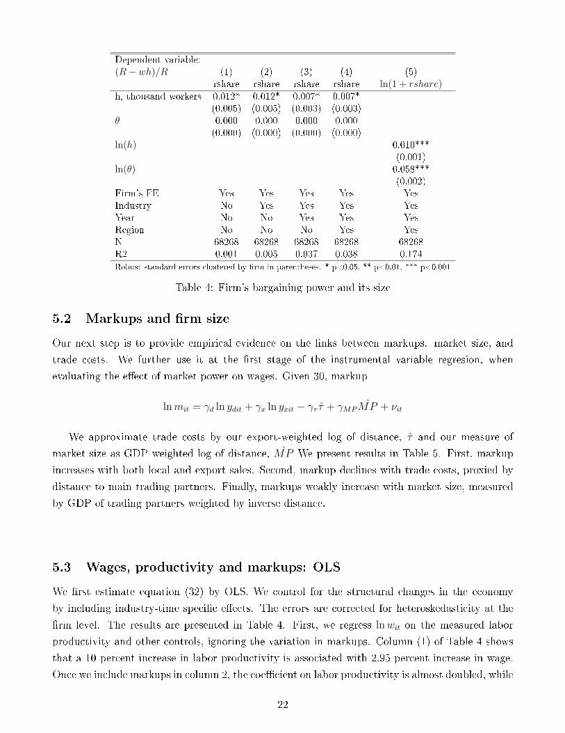
5.3 Wages, productivity and markups: OLS
We �rst estimate equation (32) by OLS. We control for the structural changes in the economy
by including industry-time speci�c e�ects. The errors are corrected for heteroskedasticity at the
�rm level. The results are presented in Table 4. First, we regress lnwit on the measured labor
productivity and other controls, ignoring the variation in markups. Column (1) of Table 4 shows
that a 10 percent increase in labor productivity is associated with 2.95 percent increase in wage.
Once we include markups in column 2, the coe�cient on labor productivity is almost doubled, while
22

Dependent variable:ln(1− c/p) (1) (2) (3) (4) (5) (6) (7) (8)ln(y) 0.213***
(0.003)ln(yd) 0.228*** 0.235*** 0.235*** 0.248*** 0.252*** 0.252*** 0.180***
(0.003) (0.003) (0.003) (0.004) (0.004) (0.004) (0.003)ln(yx) 0.188*** 0.207*** 0.207*** 0.211*** 0.215*** 0.215*** 0.145***
(0.003) (0.004) (0.004) (0.004) (0.004) (0.004) (0.003)τ -0.014*** -0.025** -0.015* -0.024** -0.026** -0.027***
(0.001) (0.008) (0.008) (0.008) (0.008) (0.007)
MP 0.003 0.002 0.004 0.004* 0.006**(0.002) (0.002) (0.002) (0.002) (0.002)
ln(θ) 0.259***(0.010)
N 74989 74989 74989 74989 74989 74989 74989 69219R2 0.277 0.288 0.289 0.289 0.329 0.333 0.335 0.358H0 : βln(yd) = βln(yx) 0.000 0.000 0.000 0.000 0.000 0.000 0.000Robust standard errors clustered by �rm in parentheses. * p<0.05, ** p<0.01, *** p<0.001
Table 5: Markups, �rm size and trade costs
the coe�cient on the markup is negative and signi�cant. Comparing results in columns (1) and (2),
points to the omitted variable bias for the model speci�cation in column (1). At the same time, the
model speci�ed in column (2) has two endogenous variables � productivity and markups � causing
an upward bias in the OLS estimation of the coe�cient on productivity, while the estimation of
the coe�cient on the markup is biased downward. Inclusion of �rm-speci�c e�ects in column (3) of
the table alleviates endogeneity problem, resulting in the coe�cient on labor productivity almost
the same as in column (1), but the coe�cient on the markup remains negative. Column (3) shows
that �rms that increase export to sales by a standard deviation pay a wage premium of 1.5 percent,
which is well in agreement with the theoretical predictions. Adding an interaction between export
status and productivity, exportit × ln θit, in column (4) demonstrates that elasticity of wage with
respect to productivity is statistically di�erent for exporters and non-exporters. At the same time
exporter wage premium more than doubles.
Results in column 4 also indicate that �rms that start importing some of their inputs pay 3.4
percent more, which corresponds well with Amiti and Davis (2012), who found 3.2 percent increase
in wage after the �rm starts importing in Indonesia. Firms that switch ownership from domestic
to foreign pay 3.5 percent higher wages. Exiting �rms pay 7.4 percent lower wage. We also have
found a positive scale e�ect, measured by total employment, even after controlling for productivity,
market power, and export status.
Columns (5) - (8) of Table 4 show results of the regression of lnwit on TFP and other controls.
The results with two di�erent productivity measures are quite similar for exogenous controls.
However, the positive e�ect of TFP on wages and the negative e�ect of markup on wages are
somewhat smaller in the absolute value. These results are expected because the model with labor
23

Dependent variable:ln(wit) Labor productivity TFP
OLS Markups FE Exp × OLS Markups FE Exp ×prod. prod.
(1) (2) (3) (4) (5) (6) (7) (8)
ln θit 0.295*** 0.398*** 0.231*** 0.226*** 0.325*** 0.362*** 0.252*** 0.232***(0.009) (0.014) (0.017) (0.016) (0.007) (0.008) (0.008) (0.008)
ln(mit) -0.294*** -0.199*** -0.199*** -0.089*** -0.118*** -0.125***(0.012) (0.012) (0.012) (0.006) (0.006) (0.007)
ln θit× -0.011 -0.031***lnmit (0.024) (0.005)Export to salesit 0.104*** 0.098*** 0.064*** 0.151*** 0.085*** 0.078*** 0.075*** 0.085***
(0.014) (0.013) (0.014) (0.041) (0.016) (0.016) (0.015) (0.016)Exportit× -0.036* -0.031***ln θit (0.016) (0.005)Importerit -0.024* -0.005 0.033*** 0.034*** 0.086*** 0.102*** 0.048*** 0.051***
(0.010) (0.010) (0.005) (0.005) (0.009) (0.009) (0.005) (0.005)Foreignit 0.123*** 0.110*** 0.034* 0.035** 0.194*** 0.196*** 0.059*** 0.059***
(0.013) (0.012) (0.013) (0.013) (0.015) (0.015) (0.014) (0.014)ln(hit) 0.118*** 0.118*** 0.049*** 0.049*** 0.133*** 0.134*** 0.033*** 0.032***
(0.003) (0.003) (0.007) (0.007) (0.004) (0.004) (0.007) (0.007)Exitit -0.062*** -0.125*** -0.073*** -0.074*** -0.156*** -0.183*** -0.103*** -0.103***
(0.015) (0.014) (0.014) (0.014) (0.017) (0.017) (0.016) (0.016)Urbani 0.074*** 0.069*** -0.010 -0.008 0.104*** 0.105*** 0.010 0.011
(0.008) (0.007) (0.022) (0.022) (0.009) (0.009) (0.023) (0.023)Industry × Year FE Yes Yes Yes Yes Yes Yes Yes YesRegion FE Yes Yes Yes Yes Yes Yes Yes YesFirm FE No No Yes Yes No No Yes YesObservations 72045 72045 72045 72045 69219 69219 69219 69219R2 0.578 0.630 0.546 0.548 0.503 0.509 0.510 0.514Standard errors clustered by �rms in parentheses. * p<0.05, ** p<0.01, *** p<0.001
Standard errors in parentheses
Table 6: OLS
productivity overestimates productivity for �rms with high value of capital, leading to a positive
correlation of errors with productivity and negative correlation of errors with markups.
5.4 Wages, productivity and markups: IV results
In this section we report results of the estimation of equation (32) by the IV GMM method in the
�rst di�erences in order to account for �rms' �xed e�ects. We use four instruments. Two of them
� services liberalization measured by EBRD indices of reforms and the input tari� liberalization
measure, which are computed according to equations (47) and (48) � instrument for endogeneity
of productivity measures. The other two � the weighted average of distances to �ve major des-
tination countries weighted by export shares and the export-weighted GDP per exporting �rm �
are instruments for markups. The errors are corrected for heteroskedasticity at the �rm level, all
regressions include industry-time and regional �xed e�ects.
The results are presented in Table 5 for the labor productivity measure and in Table 6 for
24

the TFP measure. The estimation is performed on the restricted sample. Column (1) of Table 5
presents the benchmark OLS results, which do not di�er considerably from the results estimated
on the full sample in column (3) of Table 4. Column (2) presents point estimates of the coe�cients
estimated by the instrumental variables GMM method. Relative to the results in column (1), the
coe�cient on labor productivity loses its signi�cance, while the coe�cient on the markup �ips the
sign. It con�rms our theoretical priors that the OLS estimation of the coe�cient on productivity
is biased upward and the OLS estimation of the coe�cient on the markup is biased downward.
This result holds for any model speci�cation and for any productivity measure, that are presented
in Tables 5 and 6. The sizes of the coe�cients on productivity and markups are remarkable stable.
For the baseline model in column 2 of Table 5, a 10 percent increase in labor productivity leads to
0.64 percent increase in wage, while a 10 percent increase in the markup leads to a 1.58 percent
increase in wage.
Wage is an increasing function of export to sales. Increasing exports to sales ratio by a standard
deviation increases wage by 1.4 percent. Firms that start importing their inputs pay 2.1 percent
higher wages. Firms that switch to foreign ownership start paying slightly higher wage, but the
e�ect is not signi�cant. Elasticity of wage with respect to employment within a �rm is negative
and signi�cant 0.048. Firms that move to urban areas pay slightly higher wage but the e�ect is
not signi�cant.
In column (3) we include an interaction term exportit× ln θit. Elasticity of wage with respect to
productivity is not statistically di�erent for exporters and non-exporters. It should be noted that
private �rms in Ukraine pay part of the salary in cash and do not report it as the wage bill to evade
the social security tax ranging from 32.6 to 49.7 percent of the wage bill. State-owned companies
do not have this incentive, reporting all labor-related expenses in wage bills. This feature of the
tax system leads to under-reporting of wages by the private companies and can bias our results.
Column (4) reports the results with additional variable that control for state- vs. private-owned
�rms. Privatized �rms increase wages by 9.3 percent, but it does not change our main conclusions.
Literature emphasizes distinction between multi-plant and single-plant �rms. Related to this,
distinction between multi-product and single-product �rms is important when modeling �rm's
reaction to trade liberalization (Bernard et al., 2011). We control for single- vs. multi-plant �rms
in column (5), which has no impact on our conclusions. In column (6) we control for new entrants,
which on average pay 7.3 percent lower wages than incumbents. Finally, in column (7) we include
all additional controls, but it does not change our results.
Our identi�cation strategy would fail if exclusion restrictions are not valid. For instance, trade
and services liberalization can have a general equilibrium e�ect on wages which in�uences more
�rms that use imported goods and liberalized services more intensively. In that case our excluded
variables in�uence wages not only through productivity, but also directly. We are quite con�dent
that our estimation is valid for several reasons. First, we control for the industry-time speci�c
trends directly. Second, the overidenti�cation test does not reject validity of our instruments. To
25

sum up, we �nd a robust positive e�ect of market power on wages, with elasticity in the range
0.158-0.163. The labor productivity also positively contributes to wages, but the e�ect is weaker
and is not statistically signi�cant.
As a robustness check, Table 6 reports IV results with productivity measured by TFP. In
general, results are very similar to the results discussed for labor productivity. This gives us reas-
surance that the result does not depend on the way productivity is estimated or on the speci�cation
of production technology in the model.
5.5 Wage inequality, productivity and markups: Industry level results
Having con�rmed the positive causal e�ect from market power to wages, we further test predictions
of HIR at industry level. We aggregate our data to the level of NACE 3 digit sub-industries. We
proxy ρ = θd/θx by the share of exporters, Nxjt/Njt, where N
xjt is the number of exporters and
Njt is the total number of �rms in sub-industry j at time t. Figure 1 presents a scatterplot of
the average wage as a function of the share of exporters. The solid line is the quadratic �t that
minimizes the total sum of squared errors of the following optimization
mincm,αm,βm
[∑j,t
(lnwjt − cm − αmexpsharejt − βmexpshare2jt)
2
].
With the exception of few outliers close to zero, the average wage increases with the share of
exporters within the sub-industry.
Figure 2 presents a scatterplot of the coe�cient of variation, cv(lnwjt) =σ(lnwjt)
E(lnwjt), as a function
of the share of exporters. The solid line is the quadratic �t that minimizes the total sum of squared
errors of the following optimization
minccv ,αcv ,βcv
[∑j,t
(cv(lnwjt)− csd − αsdexpsharejt − βsdexpshare2jt)
2
].
As predicted by the HIR model, the coe�cient of variation of wages within a sub-industry is �rst
rising and then declining with the increase in trade openness.
26

Dependent variable:lnωit (1) (2) (3) (4) (5) (6) (7)
OLS Base Inter- Private Single Entry Allaction plant
D.ln θit 0.149*** 0.064 0.056 0.064 0.064 0.056 0.048(0.006) (0.045) (0.043) (0.045) (0.045) (0.046) (0.044)
D.lnmit -0.146*** 0.158*** 0.158*** 0.158*** 0.158*** 0.162*** 0.163***(0.011) (0.046) (0.047) (0.046) (0.046) (0.046) (0.047)
D.Export to salesit 0.068*** 0.050** 0.122 0.049** 0.050** 0.050** 0.105(0.015) (0.017) (0.095) (0.017) (0.017) (0.017) (0.097)
D.Importerit 0.027*** 0.021*** 0.021*** 0.021*** 0.021*** 0.021*** 0.021***(0.004) (0.005) (0.005) (0.005) (0.005) (0.005) (0.005)
D.Foreignit 0.041** 0.019 0.020 0.019 0.019 0.019 0.020(0.014) (0.012) (0.012) (0.012) (0.012) (0.012) (0.012)
D.lnhit -0.000 -0.048*** -0.050*** -0.048*** -0.048*** -0.055*** -0.057***(0.010) (0.014) (0.014) (0.014) (0.014) (0.015) (0.014)
D.Exitit -0.075*** -0.050* -0.052* -0.050* -0.050* -0.053* -0.055*(0.018) (0.022) (0.022) (0.022) (0.022) (0.022) (0.022)
D.Urbani 0.024 0.013 0.013 0.012 0.013 0.013 0.013(0.019) (0.017) (0.017) (0.017) (0.017) (0.017) (0.017)
D.Exporterit× -0.030 -0.024ln θit (0.042) (0.043)D.Privateit 0.093** 0.093**
(0.034) (0.034)D.Single plantit 0.012 0.011
(0.009) (0.009)D.Entryit -0.073*** -0.076***
(0.020) (0.019)Industry × Year FE Yes Yes Yes Yes Yes Yes YesRegion FE Yes Yes Yes Yes Yes Yes YesObservations 31336 29076 29076 29076 29076 29076 29076Hansen J statistics 1.455 1.741 1.531 1.473 1.360 1.672p-value 0.483 0.419 0.465 0.479 0.507 0.433R2 0.159 0.179 0.181 0.179 0.179 0.177 0.177Standard errors clustered by �rms are reported in parentheses. * p<0.05, ** p<0.01, *** p<0.001
Notes: Dependent variable is D.ln(wi,t). Productivity and markup are instrumented by EBRD index of services liberalization, index
of trade liberalization, weighted average of distances to �ve major destination countries weighted by export shares, and by the number
of destination countries per exporting �rm.
Table 7: IV: Labor productivity
27
Dependent variable:lnωit (1) (2) (3) (4) (5) (6) (7)
OLS Base Inter- Private Single Entry Allaction plant
D.ln θit 0.152*** 0.069 0.075 0.069 0.069 0.064 0.069(0.009) (0.044) (0.044) (0.043) (0.044) (0.044) (0.044)
D.lnmit -0.074*** 0.205*** 0.204*** 0.205*** 0.205*** 0.202*** 0.202***(0.009) (0.040) (0.038) (0.040) (0.040) (0.039) (0.038)
D.Export to salesit 0.077*** 0.047** 0.063** 0.046** 0.047** 0.047** 0.061**(0.015) (0.018) (0.021) (0.018) (0.018) (0.018) (0.021)
D.Importerit 0.029*** 0.020*** 0.020*** 0.020*** 0.020*** 0.020*** 0.020***(0.004) (0.005) (0.005) (0.005) (0.005) (0.005) (0.005)
D.Foreignit 0.044** 0.023 0.023 0.023 0.023 0.023 0.023(0.014) (0.013) (0.013) (0.013) (0.013) (0.013) (0.013)
D.lnLit -0.022* -0.067*** -0.067*** -0.067*** -0.067*** -0.071*** -0.071***(0.010) (0.012) (0.012) (0.012) (0.012) (0.012) (0.012)
D.Exitit -0.109*** -0.058* -0.058* -0.058* -0.058* -0.060* -0.060*(0.019) (0.024) (0.024) (0.024) (0.024) (0.024) (0.023)
D.Urbani 0.024 0.014 0.014 0.013 0.014 0.014 0.014(0.021) (0.018) (0.018) (0.018) (0.018) (0.018) (0.018)
D.Exporterit× -0.024 -0.022ln θit (0.023) (0.023)D.Privateit 0.085* 0.086**
(0.033) (0.033)D.Single plantit -0.001 -0.002
(0.009) (0.009)D.Entryit -0.061*** -0.062***
(0.017) (0.017)Industry × Year FE Yes Yes Yes Yes Yes Yes YesRegion FE Yes Yes Yes Yes Yes Yes YesObservations 32325 30071 30071 30071 30071 30071 30071Hansen J statistics 4.731 4.468 4.827 4.729 4.499 4.350p-value 0.094 0.107 0.089 0.094 0.105 0.114R2 0.098 0.095 0.096 0.096 0.095 0.101 0.101Standard errors clustered by �rms are reported in parentheses. * p<0.05, ** p<0.01, *** p<0.001
Notes: Dependent variable is D.ln(wi,t). Productivity and markup are instrumented by EBRD index of services liberalization, index
of trade liberalization, weighted average of distances to �ve major destination countries weighted by export shares, and by the number
of destination countries per exporting �rm.
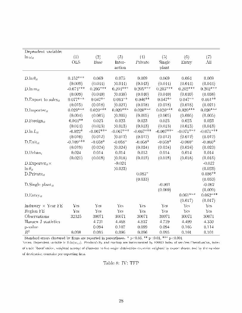
Table 8: IV: TFP
28

Figure 3: Average wage and share of exporters
29

Figure 4: Coe�cient of variation and trade openness
30

The observed regularities might be driven by variation of wages across industries and by other
factors. To test the predictions on the relationship between sub-industry wage statistics and trade
openness, we estimate the following equations
lnwjt = cm + ηm ln θjt + αmexpsharejt + βmexpshare2jt +Xjtγ
m + ujt
sd(lnw)jt = csd + ηsdσ(ln θ)jt + αsdexpsharejt + βsdexpshare2jt +Xjtγ
sd + vjt
and
cv(lnw)jt = ccv + ηcvσ(ln θ)jt + αcvexpsharejt + βcvexpshare2jt +Xjtγ
cv + vjt
where sd(lnw)jt and cv(lnw)jt are standard deviation and coe�cient of variation of wages within
the sub-industry j at time t. We estimate these equations with and without sub-industry �xed
e�ects (sub-industry is de�ned according to 3 digit NACE classi�cation), to explore the relation-
ship within and between industries. The results presented in Panel A of Table 7 indicate that
the average wage within sub-industry is positively linked to average productivity, while higher
variation of wages within industry is positively linked to variation of productivity. The coe�cients
of exporter share and exporter share squared have expected signs and are signi�cant in almost all
speci�cations. Overall, we can conclude that the results do not reject the hypothesis on inverse
U-shaped relationship between trade openness in the industry and variation of wages.
However, as Panel B of Table 7 indicates, the variation of wages within an industry is mostly
explained by the variation in markups, because the coe�cient on the variation of productivity
becomes insigni�cant, while the coe�cient on the variation of markups is positive and signi�cant.
6 Conclusions
We have studied the impact of �rm's technological e�ciency and market power on wages. Our
empirical analysis was based on a new theoretical model that brings together labor market im-
perfections, �rms' heterogeneity, and variable markups. We have found that the market structure
channel plays an important role in shaping the wage distribution within manufacturing industries.
Firms with more market power pay higher wages, while the productivity channel is weaker and is
not robustly signi�cant. The elasticity of wage with respect to TFP is 0.064, while the elasticity
of wage with respect to markup is 0.158 in the baseline speci�cation for the labor productivity.
The positive sign of the markup coe�cient indicates that the elasticity of aggregate demand is
decreasing function of output. This result is robust to the measure of productivity and to the
assumptions about the production function.
31

Dependent variable Average wagejt St. Dev. Wagejt Coef. Var. Wagejt(1) (2) (3) (4) (5) (6)OLS FE OLS FE OLS FEA.Without markups
ln θjt 0.055*** 0.217***(0.008) (0.042)
σ(ln θjt) 0.124*** 0.080*** 0.042* 0.039*(0.026) (0.023) (0.017) (0.019)
Share of exportersjt -0.636** -0.414 0.577*** 0.536*** 0.329** 0.240(0.234) (0.228) (0.092) (0.101) (0.112) (0.122)
Share of exporters2jt 0.594** 0.359 -0.587*** -0.526*** -0.352*** -0.268*
(0.227) (0.205) (0.087) (0.092) (0.102) (0.112)Share of importersjt -0.023 0.185 0.112* 0.134** 0.027 0.015
(0.105) (0.104) (0.044) (0.049) (0.043) (0.053)Share of foreignjt 0.776*** 0.522*** 0.156*** 0.169*** -0.007 -0.016
(0.099) (0.085) (0.033) (0.037) (0.022) (0.029)ln(Ljt) 0.095*** 0.055** -0.054*** -0.066*** -0.045*** -0.044***
(0.017) (0.018) (0.008) (0.009) (0.006) (0.008)Share of exiting �rmsjt -1.014*** -0.849** 0.118 0.122 0.367 0.331
(0.224) (0.265) (0.158) (0.152) (0.218) (0.225)Share of urbanjt 0.140 0.162 0.010 0.175*** -0.008 0.093
(0.076) (0.093) (0.032) (0.047) (0.024) (0.047)Sub-Industry FE No Yes No Yes No YesObservations 719 719 719 719 719 719R2 0.351 0.551 0.323 0.487 0.309 0.355
B. Including markupsln θjt 0.055*** 0.343***
(0.008) (0.043)σ(ln θjt) 0.056 0.014 -0.052 -0.058
(0.036) (0.032) (0.044) (0.045)lnmjt 0.034 -0.167***
(0.025) (0.033)σ(lnmjt) 0.106** 0.107** 0.148** 0.157**
(0.037) (0.035) (0.053) (0.058)Share of exportersjt -0.668** -0.356 0.518*** 0.439*** 0.247* 0.098
(0.240) (0.220) (0.091) (0.098) (0.100) (0.109)Share of exporters2
jt 0.650** 0.264 -0.499*** -0.419*** -0.230* -0.111(0.231) (0.198) (0.085) (0.089) (0.092) (0.101)
Share of importersjt -0.065 0.373*** 0.082 0.095* -0.015 -0.042(0.105) (0.096) (0.043) (0.046) (0.038) (0.041)
Share of foreignjt 0.759*** 0.521*** 0.158*** 0.170*** -0.006 -0.016(0.099) (0.082) (0.032) (0.037) (0.020) (0.026)
ln(Ljt) 0.098*** 0.032 -0.048*** -0.055*** -0.037*** -0.027***(0.016) (0.018) (0.008) (0.009) (0.006) (0.007)
Share of exiting �rmsjt -1.052*** -0.700** 0.025 0.044 0.238 0.215(0.233) (0.219) (0.127) (0.126) (0.145) (0.152)
Share of urbanjt 0.135 0.144 -0.002 0.161*** -0.024 0.071*(0.076) (0.091) (0.031) (0.042) (0.022) (0.036)
Sub-Industry FE No Yes No Yes No YesObservations 719 719 719 719 719 719R2 0.354 0.578 0.358 0.519 0.405 0.452Standard errors clustered by industries in parentheses. * p<0.05, ** p<0.01, *** p<0.001
Table 9: Sub-industry (NACE 3 digit) level results
32

Firms that increase export to sales by a standard deviation pay a wage premium of 1.4 percent in
our baseline IV result based on labor productivity. This channel can be one of the important drivers
of the increasing wage gap between high- and low-paid jobs, observed in the last two decades in
both developed and developing countries. We also con�rm that the e�ect of the extensive margins
of trade on wage inequality has a bell-shaped form, which is consistent with the theoretical model
developed by Helpman et al. (2010). From the methodological point, we demonstrate that the OLS
estimation of the wage-productivity relationship is biased. The suggested IV approach, which also
corrects for the measurement error, allows to eliminate the bias. Finally, based on the industry-
level analysis, we �nd evidence supporting the bell-shaped relationship between the coe�cient of
variation of wages and the share of exporting �rms in the industry.
References
Akerlof, G. and Yellen, J. (1990). The fair wage-e�ort hypothesis and unemployment. The Quar-
terly Journal of Economics, 105(2):255�283.
Amiti, M. and Davis, D. (2012). Trade, �rms, and wages: Theory and evidence. The Review of
Economic Studies, 79(1):1�36.
Amiti, M. and Konings, J. (2007). Trade liberalization, intermediate inputs, and productivity:
Evidence from indonesia. American Economic Review, 97(5):1611 � 1638.
Arnold, J., Javorcik, B., and Mattoo, A. (2011). Does services liberalization bene�t manufacturing
�rms?: Evidence from the czech republic. Journal of International Economics, 85(1):136�146.
Behrens, K. and Murata, Y. (2007). General equilibrium models of monopolistic competition: a
new approach. Journal of Economic Theory, 136(1):776�787.
Bernard, A., Redding, S., and Schott, P. (2011). Multiproduct �rms and trade liberalization. The
Quarterly Journal of Economics, 126(3):1271�1318.
De Loecker, J. (2011). Product di�erentiation, multiproduct �rms, and estimating the impact of
trade liberalization on productivity. Econometrica, 79(5):1407�1451.
De Loecker, J., Goldberg, P., Khandelwal, A., and Pavcnik, N. (2012). Prices, markups and trade
reform. Technical report, National Bureau of Economic Research.
De Loecker, J. and Warzynski, F. (2012). Markups and �rm-level export status. American Eco-
nomic Review, 102(6):2437�2471.
Dunne, T., Foster, L., Haltiwanger, J., and Troske, K. (2004). Wage and productivity dispersion
in united states manufacturing: The role of computer investment. Journal of Labor Economics,
22(2):397�429.
33

Egger, H. and Kreickemeier, U. (2012). Fairness, trade, and inequality. Journal of International
Economics, 86(2):184 � 196.
Felbermayr, G., Prat, J., and Schmerer, H. (2011). Globalization and labor market outcomes: wage
bargaining, search frictions, and �rm heterogeneity. Journal of Economic Theory, 146(1):39�73.
Fernandes, A. M. and Paunov, C. (2011). Foreign direct investment in services and manufacturing
productivity: Evidence for chile. Journal of Development Economics, In Press, Corrected Proof:�
.
Foster, L., Haltiwanger, J., and Syverson, C. (2008). Reallocation, �rm turnover, and e�ciency:
Selection on productivity or pro�tability? American Economic Review, 98(1):394�425.
Goldberg, P. and Pavcnik, N. (2007). Distributional e�ects of globalization in developing countries.
Journal of Economic Literature, 45:39�82.
Helpman, E., Itskhoki, O., and Redding, S. (2010). Inequality and unemployment in a global
economy. Econometrica, 78(4):1239�1283.
Khandelwal, A. and Topalova, P. (2011). Trade liberalization and �rm productivity: The case of
india. Review of Economics and Statistics, forthcoming.
Klenow, P. J. and Willis, J. L. (2006). Real rigidities and nominal price changes. Research Division,
Federal Reserve Bank of Kansas City.
Nakamura, E. and Zerom, D. (2010). Accounting for incomplete pass-through. The Review of
Economic Studies, 77(3):1192�1230.
OECD (2012). Divided We Stand Why Inequality Keeps Rising: Why Inequality Keeps Rising.
OECD Publishing, Paris.
Olley, G. S. and Pakes, A. (1996). The dynamics of productivity in the telecommunications
equipment industry. Econometrica, 64(6):1263 � 1297.
Shepotylo, O. and Vakhitov, V. (2012). Services liberalization and productivity of manufacturing
�rms: evidence from ukraine. Policy Research Working Paper Series.
Stole, L. A. and Zwiebel, J. (1996). Intra-�rm bargaining under non-binding contracts. The Review
of Economic Studies, 63(3):375�410.
Syverson, C. (2004). Market structure and productivity: A concrete example. Journal of Political
Economy, 112(6).
Zhelobodko, E., Kokovin, S., Parenti, M., and Thisse, J.-F. (2012). Monopolistic competition:
Beyond the constant elasticity of substitution. Econometrica, 80(6):2765�2784.
34

Appendix
Appendix 1. Mathematical proofs
Derivation of (14).
Multiplying both sides of (13) by h yields
h∂R
∂h= 2wh+
∂w
∂hh2 =
∂
∂h
(wh2
).
Integrating across [0, h] and applying integration by parts, we obtain
w =1
h2
hˆ
0
∂R
∂ξξdξ =
R(h, θ, a)
h− 1
h2
hˆ
0
R(ξ, θ, a)dξ. (49)
Multiplying both sides by h, we come to (14). Q.E.D.
Proof of Claim 1. Di�erentiating (49) in h, we get
∂w
∂h=
1
h2
h∂R∂h− 2R(h, θ, a) +
2
h
hˆ
0
R(ξ, θ, a)dξ
=∂2
∂h2
1
h
hˆ
0
R(ξ, θ, a)dξ
. (50)
It remains to prove that revenue R(h, θ, a) is concave in h if and only if 1h
´ h0R(ξ, θ, a)dξ is
concave in h.
To prove the �if� part, we assume that R(h, θ, a) is concave in h. Then, by Jensen's inequality,
for any α ∈ [0, 1] and for any h1, h2 > 0 we have
1
m
m∑j=1
R
(j
m(αh1 + (1− α)h2) , θ, a
)≥ α
m
m∑j=1
R
(jh1
m, θ, a
)+
1− αm
m∑j=1
R
(jh2
m, θ, a
). (51)
Under m→∞, (51) becomes
1
αh1 + (1− α)h2
αh1+(1−α)h2ˆ
0
R(ξ, θ, a)dξ ≥ α
h1
h1ˆ
0
R(ξ, θ, a)dξ +1− αh2
h2ˆ
0
R(ξ, θ, a)dξ,
which means that 1h
´ h0R(ξ, θ, a)dξ is concave. This completes the proof of the �if� part.
As for the �only if� part, we prove it by reductio ad absurdum. Namely, assume that 1h
´ h0R(ξ, θ, a)dξ
is concave in h, while R(h, θ, a) is not. Then, it must be that R(h, θ, a) is strictly convex in h over
some non-degenerate segment [h, h]. This implies that if we choose h1, h2 ∈ [h, h], the opposite of
(51) holds. Consequently, when m→∞, we have
35

1
αh1 + (1− α)h2
αh1+(1−α)h2ˆ
0
R(ξ, θ, a)dξ <α
h1
h1ˆ
0
R(ξ, θ, a)dξ +1− αh2
h2ˆ
0
R(ξ, θ, a)dξ.
This, however, violates the assumption that 1h
´ h0R(ξ, θ, a)dξ is concave. Thus, we come to a
contradiction, and the �only if� part is proven.
Using (50), we conclude that ∂w/∂h has the same sign as ∂2R/∂h2, which implies Claim 1.
Q.E.D.
Derivation of (17). Di�erentiating (16) with respect to h yields
∂β
∂h=
´ h0R(ξ, θ, a)dξ
h2R(h, θ, a)
[hR(h, θ, a)−
´ h0R(ξ, θ, a)dξ´ h
0R(ξ, θ, a)dξ
− ∂R(h, θ, a)
∂h
h
R(h, θ, a)
].
Combining this with (16) and using integration by parts, we obtain
Eh(β) =hR(h, θ, a)−
´ h0R(ξ, θ, a)dξ´ h
0R(ξ, θ, a)dξ
− Eh(R) =
´ h0ξ · [∂R(ξ, θ, a)/∂ξ] dξ´ h
0R(ξ, θ, a)dξ
− Eh(R).
Since ξ · [∂R(ξ, θ, a)/∂ξ] = Eξ(R)R(ξ, θ, a), we come to (17). Q.E.D.
Appendix 2. Mapping EBRD indices to services sub-sectors
For four services sub-sectors � Transport, Telecom, Finance, and Other business-related services
(hotels and restaurants, real estate, rent, informatization, R&D, agencies) � we map the sub-sector
with EBRD indices of reforms as follows:
I: Transportation 1/2(rail + roads)
I1: Telecom (telecom)
J: Finance 1/2(banking + �nancial )
H+K: Other business-related services (hotels and restaurants, real estate, rent, informatiza-
tion, R&D, agencies) 1/5( small scale privatization + price liberalization + trade liberalization+
competition reform+ �nancial reform)
36