This PDF is a selection from an out-of-print volume from the NationalBureau of Economic Research

Volume Title: Wages and Labor Markets in the United States, 1820-1860

Volume Author/Editor: Robert A. Margo

Volume Publisher: University of Chicago Press

Volume ISBN: 0-226-50507-3

Volume URL: http://www.nber.org/books/marg00-1

Publication Date: January 2000

Chapter Title: Wages in California during the Gold Rush

Chapter Author: Robert A. Margo

Chapter URL: http://www.nber.org/chapters/c11514

Chapter pages in book: (p. 119 - 141)

Wages in California duringthe Gold Rush

This chapter examines the labor market implications of a specific event—the California Gold Rush of the late 1840s and early 1850s. From thestandpoint of studying labor market integration, the Gold Rush is an in-teresting natural experiment—an unexpected, highly localized demandshock of tremendous size that required the significant and costly realloca-tion of labor (and other mobile factors) from distant locations to a verysparsely populated region. Although it is abundantly obvious from thehistorical record that labor migrated to California in response to the dis-covery of gold, the time path of wages and labor supply has remained un-clear.

Following a recounting of the history of the California Gold Rush, thechapter develops a simple model of wage determination in a gold rusheconomy. I argue that the most likely path was an initial rise in wages,followed by a steep decline.

Similar to that in chapter 3, the analysis here uses a sample of Californiaforts drawn from the Reports of Persons and Articles Hired to estimatenominal wage series for common laborers-teamsters, artisans, and clerks.A price deflator is constructed from Berry's (1984) compilation of whole-sale prices.

The time path of real wages revealed by the Reports is consistent withthe stylized model of wage determination. Real wages rose very sharplyduring the initial phase of the rush, fell abruptly in 1852, and then re-mained roughly constant for the remainder of the decade. Although it was,by definition, a purely transitory shock, the Gold Rush appears to haveleft a permanent imprint on California wage levels. I argue that the per-manent effect occurred because, as a result of the Gold Rush, California

119

120 Chapter 6

became integrated into the economy of the Northern United States, wherewages were relatively high.

The chapter concludes by examining the wage elasticity of labor supplyinto Gold Rush California over various periods of years (e.g., 1848-52),using labor quantities computed from the federal censuses and the statecensus of 1852. The estimates range between 2 and 3, suggesting a rela-tively elastic response. However, labor supply into Gold Rush Californiawas less elastic than it was into Alaska during the Pipeline era (1973-76).

6.1 The California Gold Rush

Other than the Civil War, few events in nineteenth-century Americanhistory capture the imagination like the California Gold Rush.1 The initialdiscovery of gold in 1848 and the subsequent rush of people into the statewere the subject of innumerable newspaper articles, diaries, and relatedcontemporary accounts. The Gold Rush was an epic adventure for the"argonauts" and "forty-niners" who took part in it. It has also been alightning rod for historians seeking metaphors for the grand issues offrontier development—the callous exploitation of native peoples and nat-ural resources, the slow and uncertain development of orderly govern-ment from chaos, the haphazard taming of the American West (Good-man 1994).

Although the coastal regions of California had been explored in thesixteenth century, the true origins of California settlement lie in Spain'sacquisition of French claims to the vast Louisiana territory following theend of the Seven Years' War in Europe in 1763. Charles III of Spain subse-quently sent the adventurer Jose de Galvez to push Spanish settlementnorth of Mexico, in the hope of preventing English encroachment intoMexico and its rich mining region. Galvez invented the mission—in real-ity, a colonizing institution whose purpose was to Christianize native pop-ulations, settle them into agriculture, and ultimately create an interlinkedset of local economies (Coman 1912, vol. 1; Lavender 1976, 18).

The mission approach was largely successful in Baja California andsouthern Arizona, but rebellious Indians blocked its extension into Alta(Upper) California. Galvez appointed Fray Junipero Serra to head anexpedition to Alta California, along with the governor of Baja, Gasparde Portola. After great hardship, they established a presidio (fort) at SanDiego and later one at Monterey (Lavender 1976, 19-22). By 1772, therewere five missions and two presidios. The number of missions grew slowlybut steadily. San Francisco was added in 1776, Santa Barbara in 1782(Coman 1912, vol. 1; Lotchin 1974).

Life at the missions was hard. Mortality was extremely high, agricul-tural productivity was frequently low, and there were periodic skirmisheswith Indians. Nonetheless, by the early nineteenth century, missions were

Wages in California during the Gold Rush 121

taking root, particularly in the south, where ranching and some wheatfarming flourished (Coman 1912, 1:145-55; Lavender 1976, 24-27).

The missions began to fall somewhat out of favor in the early nineteenthcentury. Conflict arose over access to land in California, and anticlericalsentiment erupted in Mexico. By the mid-18 30s, mission land was placedunder secular control, and a series of private land grants was initiated.Fueled by cheap labor, primarily Native American, southern Californiaranches had become highly profitable through cattle production, yet thestandard of living of the "working class" was miserable (Coman 1912, 1:172-89; Lavender 1976, 29-31).

Throughout its colonization of California, Mexico faced serious diffi-culties keeping out interlopers. American trappers and fur traders ap-peared in Alta California as early as 1800 (Coman 1912, 1:160). Furs weretraded for manufactured goods brought by Boston shippers who stoppedin Monterey and San Francisco on the way to China (Coman 1912,1:163-64). Russia established Fort Ross in Alta California in 1812 (illegally, butwith the full knowledge of the Mexican government) and kept it in oper-ation until 1841. By 1832, there was a well-traveled trade route betweenSante Fe and Mission San Gabriel (Coman 1912,2:214). In addition, therewas a steady stream of Americans who became Mexican citizens and prac-ticed (or promised to practice) Catholicism in exchange for land grants.By the early 1840s, they were joined by small bands of settlers (Coman1912, 2:228-41; Lavender 1976, 34, 37-40).

Slowly, but inexorably, disputes occurred between the settlers and theMexican government. In June 1846, a group of settlers staged the so-calledBear Flag Revolt (near present-day Sonoma) with the aid of Charles Fre-mont of the U.S. Corps of Topographical Engineers and sixty troops underhis command (Coman 1912, 2:246; Caughey 1948, 4-5). Word soon camethat the United States was at war with Mexico. The mission at Montereywas seized by Commodore John D. Sloat. Additional troops and navalunits were despatched from the Army of the West, the Mormon Battalion,and a contingent of poor artisan volunteers from New York who had beenpromised free passage for themselves (and their tools) if they stayed inCalifornia at the end of their tour of duty (Caughey 1948, 4-5; Lavender1976, 49). By mid-1846, the United States Navy had occupied all usableports in California (Lavender 1976, 46).

The Mexican War came to a formal end with the signing of the Treatyof Guadalupe Hidalgo on 2 February 1848. In exchange for $15 millionand the forgiveness of $3.3 million in American claims against the Mex-ican government, Mexico ceded California, New Mexico, Utah, Nevada,Arizona, and disputed parts of Texas to the United States (Lavender1976, 4).

Ironically, the treaty was signed two weeks after—and, apparently,without knowledge of—the discovery of gold that marked the formal

122 Chapter 6

beginning of the Gold Rush.2 James Marshall, a carpenter working forJohn Sutter (a recipient of a land grant from Mexico), happened on a pea-sized pellet of gold near the American River. At first, Marshall and Sutterattempted to keep knowledge of the discovery a secret, but they were un-able to prevent the information from leaking. Teamsters and other travel-ers delivered the news to various settlements on the way to San Francisco(Coman 1912, 2:256; Lavender 1976, 50-51).

The local response was rapid and extreme. According to an eyewitness,when the news reached Monterey in early May, "The blacksmith droppedhis hammer, the carpenter his plane, the mason his trowel, the farmer hissickle, the baker his loaf, and the tapster his bottle. All were off for themines. . . . [there is] only a community of women left, and a gang of pris-oners" (quoted in Lavender 1976, 51). According to a 1 June report, halfSan Francisco's population (at that time, between eight hundred and onethousand) had left for the mines, and fully three-quarters were gone bythe middle of the month (Coman 1912, 2:257; Caughey 1948, 21).

The local labor supply was supplemented by in-migration. The schoonerLouisa relayed the news to Honolulu, and other ships, bound for pointsnorth and south, did the same (Caughey 1948, 23). Migrants poured infrom Oregon (according to some reports, half the male population) andfrom Hawaii, Mexico, Chile, Peru, China, and Australia (Lavender 1976,53; Caughey 1948, 23-24; Marks 1994, 24).

The news took somewhat longer to reach the East. The first report, aletter in the New York Times, appeared in mid-August, and the New Or-leans Daily Picayune reported the discovery in mid-September (Caughey1948, 34-35). The early newspaper reports prompted disbelief, but officialarmy accounts led President Polk to make a formal announcement in De-cember (Lavender 1976, 55). Transportation companies quickly formed;handbooks for argonauts, such as George G. Foster's The Gold Regions ofCalifornia (1848), were hastily written; and an avalanche of migrants fol-lowed (Caughey 1948, 51-55).

Although the specific routes varied enormously, there were three generalways to get to California. One way was by ship around Cape Horn, thechief disadvantages being the time cost (from three to eight months) andthe hazards of shipwreck and onboard disease. A theoretically quickerroute (six to eight weeks) was to take a ship to the Isthmus of Panama,travel overland to the Pacific, and then board another ship for San Fran-cisco. Until Cornelius Vanderbilt built a railroad across the Isthmus (forwhich the fare was $25.00), the trip through Panama was extremely ardu-ous (Coman 1912, 2:261).

Another popular route was overland (Caughey 1948, 95). Migrantsbanded together in groups leaving from various points in the Midwest,such as St. Louis. Because travel during winter was next to impossible,most tried to leave in April or May at the latest, the goal being to arrive

Wages in California during the Gold Rush 123

in the gold fields by September. Overland migrants battled impassable ter-rain, bad weather, wagon damage, hunger, thirst, disease (cholera epidem-ics were frequent), and the occasional Indian attack (Caughey 1948, 58-60; Parke 1989).

Aside from the time costs, the money costs of migration were veryhigh by the standards of the time. Depending on the port, fares on the Pan-ama Route ranged from $100 to $300, for example, and the money costsof equipping an overland trip were in a similar range (Caughey 1948, 66;Parke 1989, 137). Despite the high time and money costs of transport,the numbers of migrants are impressive—an estimated eighty to ninetythousand annually in 1849 and 1850 (Wright 1940, 341-42; Lavender1976).3

Although all surely had gold on their minds, not everyone became aminer (or remained one for long). Many migrants realized that profitscould be made transporting consumer goods to the mines and set upmakeshift stores under tents at mining camps (Coman 1912, 2:274-76;Lavender 1976, 75). Others sought to make their fortune in commerce,real estate, banking, or other services in rapidly growing San Francisco(see below). By 1860, there were 217 miners for every 1,000 people in thestate, compared with 624 per 1,000 in 1850 (DeBow 1853, 976; Kennedy1864, 35).4

The immediate consequence of the in-migration was rapid popula-tion growth. Estimates of the population on the eve of the Gold Rush,excluding non-Christianized Indians, range from three to eight thousand(Coman 1912, 2:217; Caughey 1948, 2; Lavender 1976, 15). The 1850 fed-eral census put the population at ninety-three thousand, 77 percent ofwhom were males between the ages of fifteen and forty (DeBow 1853,966-68; Kennedy 1862, 130).5 By 1852, the population had grown to ap-proximately 264,000 (DeBow 1853, 982).

Although most scholars date the end of the rush sometime in the early1850s (some as late as 1857 [see Marks 1994, 31]), population growthfueled by in-migration continued through the rest of the decade, albeit ata slower pace. By 1860, the population had risen to 380,000, but the adultmale (ages fifteen to forty) share had fallen to 49 percent, indicating asubstantial shift in the demographic composition of the in-migrants to-ward more permanent settlers (Kennedy 1862,131; Kennedy 1864,26-27).

Some of the most spectacular growth occurred in San Francisco. In1844, the population of Yeuba Buena (the Mexican name for San Fran-cisco) was about fifty. A town census in 1847 showed that the hamlet hadgrown to 459 souls over the preceding three years, and the populationdoubled again the next year, presumably because of the establishmentof the quartermaster's depot and the military presence left over fromthe Mexican War (Lotchin 1974, 8). Then, as a consequence of the GoldRush the population exploded. By 1852, San Francisco housed thirty-four

124 Chapter 6

thousand inhabitants and, by 1860, fifty-six thousand (Lotchin 1974,102).External trade expanded swiftly, being surpassed during the decade onlyby that in New York, Boston, and New Orleans (Lotchin 1974, 45).

San Francisco's extraordinary growth can be attributed to two factors—direct access to the Pacific (i.e., its port facilities) and proximity to thegold fields (Coman 1912, 2:277; Lotchin 1974, 5-6). Prospective forty-niners who took the sea route arrived at San Francisco, where they soughtto buy supplies for the final leg of their journey and equipment for themines, thereby creating a booming market in pans, shovels, and Indianbaskets (Coman 1912, 2:279; Caughey 1948, 32). Miners journeyed backto the city with their treasure, where they attempted to purchase goodsand services. During the early years, most goods, including food, wereimported into San Francisco—including, evidently, turtle meat from theGalapagos Islands. Eventually, the imports gave way to locally producedagricultural and manufactured goods, most of which were marketed inSan Francisco (Lotchin 1974, 10, 47; Caughey 1948, 210-13).

In the case of certain locally produced services, the shock to demandwas sometimes so great that the line between traded and nontraded goodsblurred. The cost of washing, it is said, rose so rapidly after 1848 thatclothes and restaurant linens were sent by clipper ship to Hawaii or evenChina for cleaning (Marks 1994, 197-99).6

After the initial deposits near Sutter's Mill were exhausted, minersspread out over a thirty-five-thousand-square-mile area looking for moregold (Coman 1912, 2:266-68; Caughey 1948, 52-54). Some of the go ld-so-called placer deposits—was so easy to find that it could be literallyscooped out of streams, but other deposits were harder to locate and re-trieve.

By the second half of 1849, the easy gold nearby the mother lode wasgone, and more complex methods—using cradles, "long toms," and sluiceboxes—had to be employed. Miners discovered that mercury ("quick-silver") bonded with gold in an amalgam, which could then be cleaned.Quicksilver was readily available owing to the discovery of rich depositsnear San Jose (Lavender 1976, 62).

Although placer mining remained the most significant method of min-ing until late in the 1850s, alternatives soon appeared. Quartz mining grewafter extensive deposits were discovered near Mariposa in 1849. Stampmills, the use of hydraulics, and tunneling were other important innova-tions. By comparison with placer mining, however, the required capitalinvestments (and associated risks) of these alternative methods were sub-stantial, beyond the means of ordinary miners. Mining companies formed,and entrepreneurs competed with placer mining to hire laborers (Caughey1948, 249-66).

Wherever significant deposits were found, mining camps soon followed.By the standards of the day—and certainly by those of the twentieth cen-

Wages in California during the Gold Rush 125

tury—living conditions in the camps were extraordinarily bad. Aside frommining, there was little to do, and alcoholism was rampant. So, too, wasdisease and malnutrition, as sanitary conditions were horrible, in part ow-ing to the environmental damage caused by the mining operations and theclose (and crude) living quarters. Nonetheless, the camps thrived as minersfashioned crude local government and rudimentary procedures for enforc-ing their stakes (Caughey 1948; Lavender 1976, 65-66; Marks 1994).

Once the gold ran out, the camps were abandoned as quickly as theyhad been established (Caughey 1948, 267). Those still bitten by the goldbug moved on to the next strike or, sometimes, gold rushes elsewhere (e.g.,Australia [see Caughey 1948, 293]). The less successful sought to returnhome but, hampered by high migration costs, frequently settled for em-ployment in agriculture or in the burgeoning nonfarm sector in andaround San Francisco (Caughey 1948; Lotchin 1974; Lavender 1976).

The Gold Rush had important political consequences. By far themost important was California's early admittance into the Union in1850, thereby bypassing territorial status. A constitutional convention wascalled in 1849, and the constitution was overwhelmingly ratified by popu-lar vote on 13 November. From the standpoint of statehood, the criticalissue was slavery: Califoraians desired admittance as a free state, whichupset the delicate political balance in Washington. The furor was abatedby the Compromise of 1850, by which California was admitted as a freestate while New Mexico and Utah were organized as territories that couldthen decide for themselves whether to be slave or free (Lavender 1976,69-71).

6.2 Wage Determination in a Gold Rush Economy

This section presents a simple model of wage determination in a goldrush economy. The model is not novel—it is a standard Dutch diseaseframework, and a similar version of it has been used to analyze anotherhistorical gold rush, that of Australia in the early 1850s (Maddock andMcLean 1984).7 The prediction for nominal wages in the model economyis straightforward: nominal wages rise after the discovery of gold, thendecline once labor supply fully adjusts to the spatial shock to labor de-mand. The comparative static path followed by real wages may be morecomplex, but it is likely, too, that real wages rise initially and then fall.

As a point of departure, imagine a pre-gold rush economy, by definitionone in which population is small and perhaps highly scattered. There areN individuals, each of whom is endowed with equal shares (IIN) of theeconomy's known stocks of gold. N is fixed in the short run but may varyin the long run. Initially, I assume that known stocks of gold are verysmall; however, as the number of individuals changes, I maintain the as-sumption that each is endowed with 1/iV of the stock of gold.8 The total

126 Chapter 6

capital stock, K, is fixed in the short run, and each individual has an equalshare (1 MO of it.

Individuals maximize utility, which is defined over the consumption ofa locally produced good, X, whose price is px, and an imported good, Z.The traded good is supplied from a settled economy removed by distancefrom the gold rush economy. The supply of the traded good is assumed tobe perfectly elastic at price pz.

Individuals allocate their available labor supply (L) between the produc-tion of the local good and gold production. The production function ofthe local good is X = F{LX, K), where K is capital. Once produced, thelocal good can be either consumed or sold at the price px. Gold, as well,can be used to purchase either X or Z, but it cannot be consumed. Goldis the numeraire commodity.9

The function g is a harvesting function, which converts the stock of ore(0) into a flow (g) available for export or for purchase of X. I assume thatboth F and g are concave; g(0)S = 0 (if no labor is allocated toward goldharvesting, gold output is zero); and g ^ 1 for any value of Lg = L — Lx.

The first-order conditions are straightforward.10 Consumption of X andZ should be efficient, as should the allocation of labor between the pro-duction of the local good and the harvesting of gold: that is, labor is allo-cated to equalize the value of the marginal product in both production ac-tivities.

I model a gold rush as an increase in the economy's known stock of ore(S). An increase in S shifts the harvesting function outward, but, becauseg(0)S = 0, the shift is not a parallel one. At a fixed level of pxFL (= w,the nominal wage), individuals will want to allocate more labor to goldharvesting than in the initial equilibrium. In the aggregate, the increase inLg produces an inward shift in the supply of labor to the production ofthe local good, causing w to rise.

Gold has value in exchange, however, so the aggregate demands for Xand Z may change. As long as X is a normal good, the demand for X willincrease, leading to an increase in the demand for labor in the local goodssector. The increase in the demand for labor in the local sector furtherdrives up w and also px. Define the real wage to be w/h(px, pz), where ft isa cost-of-living function.11 Because pz is exogenous (the supply of Z isperfectly elastic), whether the real wage rises or falls depends on wlpx.However, w/px = FL. If, in the new (short-run) equilibrium, the quantityof labor demanded in the local sector declines, FL will increase, and so willthe real wage.12

In the long run, mobile factors (labor and capital) may flow in (or out)of the gold rush economy, provided that, in the new equilibrium, factorreturns are sufficiently high to justify costs of adjustment (see below). La-bor may be attracted into the gold rush economy because real income ishigher after the discovery of gold. Capital may be attracted, especially

Wages in California during the Gold Rush 127

because in-migration of labor will increase the aggregate demand for XPFor modeling purposes, I assume that any new labor shares in the endow-ment of gold equally with the initial residents. Consequently, from thestandpoint of individuals, 5 falls, and the harvesting function shifts in-ward. The inward shift reduces the incentive to mine gold, thereby increas-ing the incentive to supply labor to the local goods sector. If the laborsupply effect dominates relative to any shift in product demand, w willfall, as will w/px (and, thus, so will the real wage).

The model captures certain essential features of wage determination ina gold rush economy, but there is no question that it is highly stylized inseveral respects. For example, the model presumes that a representativeindividual allocates time to gold production and to production of the localgood. While miners often did just that over the course of the year (becausemining was seasonal [see below; and Lotchin 1974]), others clearly special-ized their labor supply. Specialization does not alter the basic thrust of themodel as long as some individuals were at the margin of shifting into goldproduction just prior to the gold discovery.14

Second, it was necessary to prospect for gold and establish a claim be-fore harvesting it. Both activities had uncertain returns. Uncertainty canbe incorporated in the model in the following manner. Assume that timespent harvesting gold is divided into two activities: prospecting (whichincludes establishing claims) and harvesting. By allocating Lp to prospect-ing, each individual can increase the probability p(Lp) that he will findgold (I assume that p" < 0). Expected income from gold harvesting is now

p(L )g(L - Lx - L)S.

There are now two ways to model a gold rush—either an increase in S oran upward shift in p for any given level of Lp. Either way, the gold rushincreases the expected marginal product of labor in gold harvesting, andthe remainder of the static analysis is unchanged.

6.2.1 Wage Dynamics

The model developed above does not directly address the dynamics ofwage adjustment in the gold rush economy. To describe the dynamics ofwage adjustment, it is necessary to specify expectations about the occur-rence and duration of the shock and about adjustment costs. In what fol-lows, I assume that the gold rush is a transitory shock—that is, the proba-bility that its duration will continue indefinitely is known, in advance, tobe zero.15 For the moment, I assume that labor is the mobile factor and,therefore, ignore capital in- (or out-) migration.

Suppose that individuals had perfect foresight that the gold rush wouldbegin at date t and last until date t' and that adjustment costs were con-vex.16 By adjustment costs, I mean all costs associated with changing the

128 Chapter 6

allocation of labor from its initial pre-gold rush equilibrium and changingit back again once the gold rush has ended.

With perfect foresight and convex adjustment costs, it would be rationalfor labor to begin migrating into the economy before the gold rush, in or-der to avoid incurring high marginal adjustment costs at date /. Similarly,it would make sense for labor supply to decline just before the end of therush, again to avoid high marginal adjustment costs. Therefore, w fallssomewhat before date /, but the influx of labor before t will generally notbe sufficient to prevent w from rising above its long-run equilibrium valuefor a while after t (Carrington 1996).17 Analogously, some excess labor willremain after t', causing a temporary slump in wages.

What if dates / and t' are uncertain but adjustment costs are zero? Byuncertain, I mean that no individual knows exactly when (or even if) agold rush will occur. Once the shock occurs, however, information that arush has begun is instantaneously available to all individuals. Similarly,the end of the rush is uncertain, but, once it has occurred, this informationis immediately transmitted.

If adjustment costs were zero, then uncertainty over t and t' has noeconomic consequence. Labor simply adjusts once the shock occurs, andwages move immediately to their new equilibrium value, returning to theiroriginal level when the rush is over.

Of course, individuals did not have perfect foresight about the discoveryof gold or the duration of the rush, and, on the basis of the discussion insection 6.1, adjustment costs were obviously nonzero. Further, as section6.1 argued, the discovery of gold took place in stages—that is, the shockwas spread through time.

If the gold discoveries were unanticipated but sequential and adjust-ment costs were convex, then wages would rise steeply during the periodof discovery, followed by an abrupt decline when the rush ended (becauseall the labor would be surplus at that point). If, as assumed above, therush were a transitory phenomenon, wages would then eventually returnto their prerush level after the rush's end. The precise pattern followed bywages during the period of discovery would depend on the size of theshocks to labor demand, their precise timing, and how quickly labor re-sponds.

Up to this point, I have ignored capital mobility. Allowing for capitalmobility (with adjustment costs) might alter dramatically the wage adjust-ment path (Taylor 1996). For example, if adjustment costs for capital wereuniformly lower than for labor, the initial jumps in wages would be greater.If the capital were of the "putty-clay" variety—capital costs are mostlysunk once the capital is in place—relatively high wages might be sustaineda while after the rush is over. However, wages would still eventually returnto their initial equilibrium, unless it was profitable for some other reasonto continue to invest in the gold rush economy after the rush was over.

Wages in California during the Gold Rush 129

More complex dynamic models could also be fashioned by consideringexactly how factor supply, particularly labor, would change in the short asopposed to the long run and by incorporating inflationary feedback. Forexample, individuals in the gold rush economy have strong incentives tosubstitute leisure intertemporally. They expand effort in the short run fol-lowing the discovery of gold, believing that the additional work will betemporary, and, having accumulated gold (a store of value), they will enjoymore leisure and possibly consumption in the future. However, given thatdaily and weekly hours of work in the late 1840s and early 1850s werealready quite high—for example, a ten-hour day and sixty-hour workweekwere not uncommon—it is unclear that increases in hours at either inten-sive margin offered much scope for substitution (Lotchin 1974, 86). Butthe same may not have been true of annual hours, in the light of the wide-spread seasonality of labor demand during the antebellum period (Enger-man and Goldin 1993).

The particular timing of migration could also be analyzed in a morecomplex model. Because gold harvesting was uncertain, individuals in thesettled economy might prefer to wait rather than migrate immediately be-cause the majority of the costs of migration were sunk once incurred.18

However, the very concept of a rush suggests that prospective migrantsbelieved that the easy gold would be gone unless they got there first.19

Given high migration costs, if the first effect dominates, labor supply willbe inelastic in the short run but might become abruptly elastic. If the sec-ond effect dominates, however, labor will rush in, but migration will even-tually tail off.

By inflationary feedback, I mean a nonneutral effect of changes in thestock of gold on wages and prices. Because the country was on a metalstandard, there is little doubt that the California Gold Rush raised thegeneral price level. But the issue here is not the general price level; it iswhether increases in the stock of gold affected local prices more quicklythan wages—that is, whether nominal wages in California were sticky inthe short run (for an analysis of nominal wage rigidity, see chap. 8). Cer-tainly, the anecdotal evidence on prices during the Gold Rush is suggestiveof the possibility of inflationary feedback (Caughey 1948, 203; Marks1994, 177).20 Unfortunately, the wage and price data at hand are notsufficient to determine whether inflationary feedback occurred, and I ig-nore the possibility in my empirical analysis.21

6.3 Data and Estimation of Wage Indices

Traditional accounts of the California Gold Rush provide anecdotalevidence on wages and prices but not the sort of quantitative basis toconstruct a continuous nominal or real wage index comparable in qualityto those presented in chapter 3.22 To construct wage indices, I make use of

130 Chapter 6

a sample of wages paid to civilians hired at United States Army installa-tions in California drawn from the Reports of Persons and Articles Hired,the same source used in chapter 3. As indicated in the discussion in section6.1, the army was present in California before the Gold Rush, and itsinstallations continued to operate during and after the discovery of gold.California forts appear to have functioned like their counterparts else-where in the country, civilians being hired to perform various tasks. Theoccupations of civilians at California forts were also similar to those atforts elsewhere in the country (e.g., laborer, teamster, artisan, clerk).

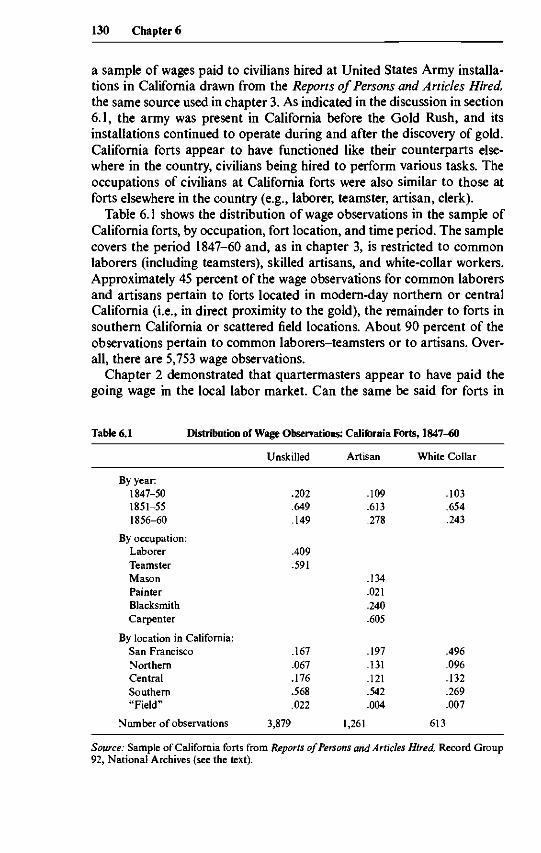
Table 6.1 shows the distribution of wage observations in the sample ofCalifornia forts, by occupation, fort location, and time period. The samplecovers the period 1847-60 and, as in chapter 3, is restricted to commonlaborers (including teamsters), skilled artisans, and white-collar workers.Approximately 45 percent of the wage observations for common laborersand artisans pertain to forts located in modern-day northern or centralCalifornia (i.e., in direct proximity to the gold), the remainder to forts insouthern California or scattered field locations. About 90 percent of theobservations pertain to common laborers-teamsters or to artisans. Over-all, there are 5,753 wage observations.

Chapter 2 demonstrated that quartermasters appear to have paid thegoing wage in the local labor market. Can the same be said for forts in

Table 6.1 Distribution of Wage Observations: California Forts, 1847-60

By year:1847-501851-551856-60

By occupation:LaborerTeamsterMasonPainterBlacksmithCarpenter

By location in California:San FranciscoNorthernCentralSouthern"Field"

Number of observations

Unskilled

.202

.649

.149

.409

.591

.167

.067

.176

.568

.022

3,879

Artisan

.109

.613

.278

.134

.021

.240

.605

.197

.131

.121

.542

.004

1,261

White Collar

.103

.654

.243

.496

.096

.132

.269

.007

613

Source: Sample of California forts from Reports of Persons and Articles Hired, Record Group92, National Archives (see the text).

Wages in California during the Gold Rush 131

California? Unfortunately, the paucity of wage data for the state makescomparisons difficult. However, it is clear from inspection of the originaldata that the wages paid at California forts were far in excess of those paidelsewhere in the United States—and, as will be demonstrated shortly, thearmy data imply that wages rose very sharply in the aftermath of the dis-covery of gold.23

6.3.1 Hedonic Wage Regressions

Like the sample analyzed in chapter 3, the California sample is not largeenough to construct occupation-specific wage series for each fort. Fewforts hired the same type of labor every year, and the numbers of observa-tions across forts varies over time. As pointed out in chapter 3, analysis ofthe data that ignored such composition effects would be misleading. Thus,following chapter 3,1 estimate hedonic wage regressions of the form

lnw = Xfi + e,

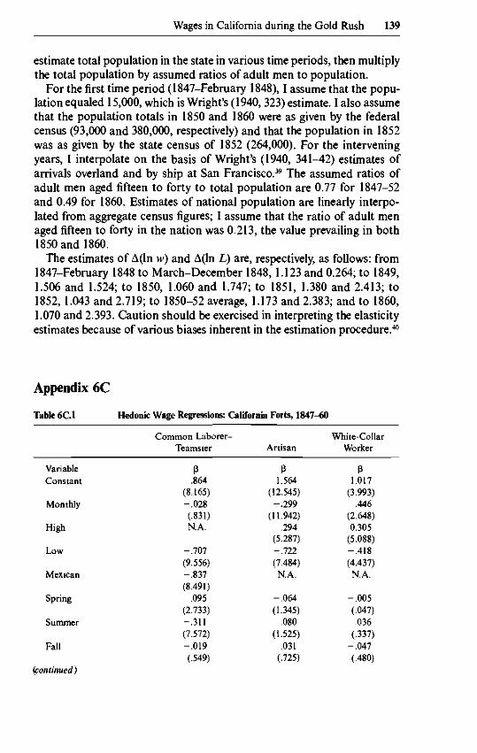
where In w is the log of the nominal daily wage, X is a vector of indepen-dent variables, the p's are the hedonic coefficients, and e is the error term.Monthly wages are converted to daily wages by dividing by twenty-sixdays per month. As in chapter 3, the independent variables are dummyvariables for fort location, characteristics of the worker or job associatedwith especially high or low wages, whether the worker was hired on amonthly basis, season of year, and time period. Separate regressions areestimated for the three occupation groups (common laborers-teamsters,artisans, and white-collar workers). The regressions are reported in appen-dix table 6C. 1.

The cross-sectional patterns revealed by the regression coefficients areinformative about the antebellum labor market in California. Seasonalvariation in wages, for example, is broadly consistent with what is knownabout seasonal fluctuations in labor demand. Summer was the slack sea-son in gold production, and miners flocked to San Francisco to find alter-native employment (Lotchin 1974, 49), while "every spring [the miners]drifted back to the diffings, leaving a shortage of labor" (Coman 1912,2:316). The seasonal lull in gold production may explain why the wages ofcommon laborers were relatively low in the summer. Artisanal wages weretemporarily higher during the summer, a prime season for constructionactivity. Rapid growth in population placed enormous strains on the con-struction sector, which needed to bid skilled labor away from the mines(Lotchin 1974, 50). This may also explain why carpenters were highly paidin California relative to other artisans, at least compared with elsewherein the United States (see chap. 3 above; and Coman 1912, 2:317). Thechoice to enter the white-collar market was not a seasonal one, and, there-fore, it is not surprising to find an absence of seasonality in clerical wages.

Despite generally high labor demand during the period, there is still

132 Chapter 6

evidence of a premium for unemployment risk, as artisans hired on amonthly basis generally earned a lower average daily wage than thosehired daily. There is no evidence of a daily wage premium for clerks—indeed, the positive coefficient of the "monthly" dummy suggests that thefew clerks hired on a daily basis were of a lower level of skill than indicatedby their occupation designation in the payrolls.

Regional patterns in money wages in California bear resemblance tothose occurring elsewhere. Skill differentials were generally lower in north-ern California than in southern California. However, the negative effect ofa southern California location may also be proxying for unobserved ethnicor racial (Native American) background. Hispanics, who were concen-trated in southern California, earned much less than other workers, andHispanic status may very well be underreported in the data.24

6.3.2 Time-Series Patterns

As in chapter 3,1 use the hedonic coefficients to estimate annual seriesof nominal daily wages for the three occupation categories. The procedureused to calculate the series is discussed in appendix 6A. In brief, the proce-dure is similar to that used in chapter 3 in that the wage series are derivedfrom hedonic indices applied to benchmark wage estimates. However, ad-ditional adjustments were deemed necessary to produce estimates for theinitial rush years of 1847-49 (for further details, see app. 6A). The nominalwage estimates are shown in appendix table 6C.2.

Consistent with the theoretical model, nominal wages rose sharply forall three groups from 1847 to 1850 (or 1851 in the case of artisans). Wagesthen declined sharply for all three occupation groups, fluctuating for theremainder of the 1850s.

The annual movements are broadly consistent with qualitative accountsof the rush. Scattered estimates of wages in newspaper articles suggest thatwages rose after the gold discoveries and remained roughly stable until1853 (Lotchin 1974, 86; Gerber 1997). My series clearly capture the steepinitial rise and subsequent decline.25 A business-cycle downturn is knownto have occurred in 1855 following a local banking panic, and this, too,apparently left its imprint in wage levels (Coman 1912, 2:285-87; Lotchin1974, 51, 59).

To convert the nominal wage series into real wage indices, it is necessaryto deflate by a price index, as in chapter 3. Data to construct a price defla-tor for antebellum California are extremely scanty, but it is possible to useBerry's (1984) compilation of prices from newspapers to construct a roughprice deflator.26

The price deflator is given in appendix table 6C.3. Although there aresevere fluctuations at annual frequencies, the general pattern is of a rise inprices during the early years of the rush, followed by an abrupt (and ap-parently persistent) decline. The short-run increase in prices is consistent

Wages in California during the Gold Rush 133

with anecdotal evidence of goods shortages during the initial phase of therush, while the subsequent decline in prices presumably reflects the dra-matic growth of the commercial sector in and around San Francisco(Caughey 1948; Lotchin 1974).27

The real wage series, formed by dividing the nominal wage estimates(indexed at 100 in 1860) by the price deflator, are shown in appendix table6C.3. The series should be viewed with caution for three reasons. The pricedata refer solely to wholesale prices, and no provision is made for housingprices. It is entirely possible that including housing prices would dampenthe short- and long-run increases in real wages evident in the indices. Therange of goods included in the price deflator is limited, even comparedwith the price deflators used in chapter 3. Berry's price data refer exclu-sively to non-southern California locations.28 However, it can be shownthat the substantive findings are similar if the wage sample is restricted tonon-southern California forts.

Despite these problems, the real wage indices essentially mimic the pat-terns evinced in the nominal wage series. Real wages of common laborersincreased by approximately 615 percent from late 1847 and early 1848 totheir peak in 1849. Because of the timing of the observations, the overallrate of increase over the same period cannot be determined for artisansand clerks, but it is clear that their real wages also grew rapidly. For ex-ample, the real wages of artisans rose by nearly 259 percent from thespring of 1848 (March-May 1848) to 1849; those of clerks rose by 189 per-cent over the same period.

Following the very steep rise, real wages fell, except for a spike in 1851caused by a sudden drop in prices that was reversed in 1852. The realwages of common laborers fell sharply in 1855 but recovered by the endof the decade to the level reached in 1852 and 1853. Similarly, the realwages of artisans and clerks in the remainder of the 1850s hovered closeto the 1860 index value of 100.

The real wage series suggest several findings. Real (and, for that matter,nominal) wages were clearly flexible during the Gold Rush; accepting theindices at face value, there can be no question that the discovery of goldmarkedly affected wages.

However, what is not consistent with the model is the finding for allthree occupations that real wages were far higher in 1860 than in 1847.The Gold Rush was a transitory shock, yet the rush appears to have leftwages permanently higher in California.

Implicit in the model was an assumption that real wages in the settledeconomy were constant over the period of the Gold Rush. The real wageindices in chapter 3 indicate that, elsewhere in the United States, realwages were higher in 1860 than in 1847. Thus, real wages could havetrended upward in California simply because they were trending upwardelsewhere.

134 Chapter 6

However, while rates of growth of real wages elsewhere were positiveover the period 1847-60, they were far lower than in California.29 In addi-tion, wage data from the 1860 Census of Social Statistics suggest that realwages in California on the eve of the Civil War were similar to average lev-els elsewhere in the country.30 If so, the clear implication is that real wagesin California just before the rush were well below real wages elsewhere inthe United States.

That real wages in California circa 1847 may have been low by Northernstandards is less paradoxical than it seems. To the extent that pre-GoldRush California was part of any regional economy at all, it was part ofthe Mexican economy, the economy of coastal points north, and, to amuch lesser extent, that of Central and South America (Wright 1940,323).31 As pointed out in section 6.1, initial in-migrants came from theselocations, and, for them, the returns to migration, on average, were surelypositive. By the time labor flows had begun to arrive from the Eastern andMidwestern United States (1849), real wages in California substantiallyexceeded those elsewhere in the United States.32

But the Gold Rush could not have left a permanent imprint on realwages unless there had been a substantial inflow of factors complementaryto labor and continued incentive to invest capital. The Yukon Gold Rushof the late 1890s did not transform southern Alaska into the equivalent ofCalifornia. What became clear to the migrants (and to many miners whostruck gold early in the rush) was that California was rich in many ways,specifically in agricultural resources. As noted in section 6.1, Californiabypassed territorial status, and statehood presumably reduced the risk ofpermanent settlement. The rapid, sustained growth of San Francisco isprima facie evidence of agglomeration effects and a widening of the mar-ket for locally produced agricultural (and manufacturing) goods (Coman1912, 2:291-314; Caughey 1948; Lotchin 1974).

Evidence of an inflow of complementary factors is both indirect anddirect. Indirect evidence of an inflow of complementary factors can begleaned from Berry (1984), who, in addition to wholesale prices, collecteda series of monthly interest rates in San Francisco. The wage-rental ratioin 1850 was less than half its value in 1860, suggesting extreme initialscarcity of capital (Coman 1912, 2:307). Translating the trend in the ratioduring the 1850s into equivalent movements along a factor price frontier,the implication is that the capital-labor ratio must have been rising.

While the extraordinarily high relative price of capital that prevailed inSan Francisco in the early 1850s may have been partly due to unusuallyhigh risk, direct evidence of capital accumulation can be found in the city's(and state's) active participation in issuing bonds in the New York andLondon financial markets (Lotchin 1974, 60-61, 77). Additional directevidence comes from the 1850 and 1860 censuses. In 1850, per capita in-vestment in manufacturing capital was negligible but, by 1860, had grown

Wages in California during the Gold Rush 135

in real terms over the decade by 1,204 percent. Investments in land clear-ing and complementary factors raised wheat output per acre by 463 per-cent over the decade.33 Capital inflows sustained the transitory wageeffects of the Gold Rush, initializing the long process by which Californiabecame an integral part of the American economy.

6.4 The Elasticity of Labor Supply into Gold Rush California

In this section, I present estimates of the elasticity of labor supply intoGold Rush California. I compare my elasticity estimates to Carrington's(1996) estimates for labor supply into Alaska during the building of theAlaska Pipeline in the mid-1970s.

The elasticity of labor supply is

eLw = d(\nL)/d(\nw),

where d indicates the difference operator. I identify d(ln L) with estimatesof the logarithm of the change in the ratio of the number of adult menbetween the ages of fifteen and forty in California relative to the aggregatepopulation in this age (and sex) group. For the purposes of the calculation,I use the real wage series for common labor in California, expressed rela-tive to the national aggregate series for common labor constructed in chap-ter 5. The calculation of the elasticity estimates is described in appendix6B, and the estimates are shown in table 6.2.

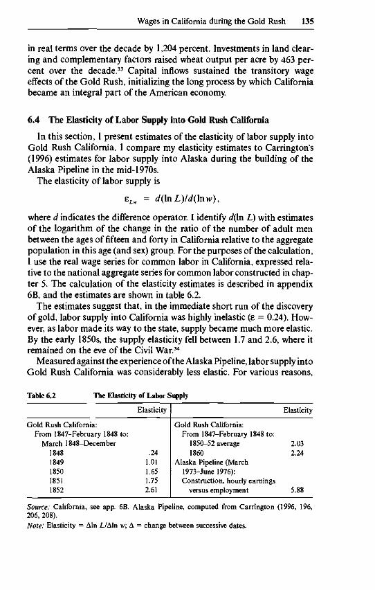
The estimates suggest that, in the immediate short run of the discoveryof gold, labor supply into California was highly inelastic (e = 0.24). How-ever, as labor made its way to the state, supply became much more elastic.By the early 1850s, the supply elasticity fell between 1.7 and 2.6, where itremained on the eve of the Civil War.34

Measured against the experience of the Alaska Pipeline, labor supply intoGold Rush California was considerably less elastic. For various reasons,

Table 6.2 The Elasticity of Labor Supply

Gold Rush California:From 1847-February 1848 to:

March 1848-December18481849185018511852

Elasticity

.241.011.651.752.61

Gold Rush California:From 1847-February 1848 to:

1850-52 average1860

Alaska Pipeline (March1973-June 1976):Construction, hourly earnings

versus employment

Elasticity

2.032.24

5.88

Source: California, see app. 6B. Alaska Pipeline, computed from Carrington (1996, 196,206, 208).Note: Elasticity = Aln L/Aln w; A = change between successive dates.

136 Chapter 6

direct comparisons between the Gold Rush and the Pipeline labor supplyare difficult to make, but, on the assumption that daily hours were notthe primary intensive margin during the rush, the relevant comparison isCarrington's (1996) estimate for Pipeline construction workers, as com-puted from changes in total employment and hourly wages, eLw = 5.88(see table 6.2).35 In the case of the Pipeline, the period covered is March1973-June 1976, or three and a half years. By this standard, labor supplyinto Alaska during the Pipeline era was roughly three times as elastic aslabor supply into California during the Gold Rush.

That labor was more elastically supplied during the Pipeline era is nottoo difficult to rationalize. The Alaska Pipeline was a project of knownduration, in which the shock to local labor demand was fully anticipatedand the returns to migration were essentially known ex ante. By contrast,the discovery of gold was unanticipated, the duration of the Gold Rushwas unknown ex ante, and the returns to migration were highly uncer-tain.36 More fundamentally, vast improvements in internal transportationand in access to economic information across regions in the 125 yearsbetween the Gold Rush and the Pipeline era dramatically reduced migra-tion costs for the prospective worker on the Alaska Pipeline, comparedwith the costs faced by the prospective argonaut.37

6.5 Conclusion

This chapter has examined how the antebellum economy coped with avery large, highly localized shock to the demand for labor—the CaliforniaGold Rush. A simple model of wage determination, in which real wagesrose sharply during the initial stages of the rush and subsequently de-clined, fit the data reasonably well. However, the rush was far more thana transitory phenomenon for it left California wage levels permanentlyhigher. Americans became convinced that the Golden State held riches farbeyond the nuggets found at Sutter's Mill. Capital poured into California,sustaining wages after the rush ended. Newly minted as a state, Californialeft behind its Hispanic economic heritage to become part of the high-wage American economy.

Appendix 6A

Construction of Nominal Wage Estimates

Estimates for 1847-60

This appendix describes the construction of the nominal wage estimatesfor California from 1847 to 1860.

Wages in California during the Gold Rush 137

Common Laborers

The 1860 estimate ($2.62) is the value reported for California in the1860 Census of Social Statistics. I use 1860 rather than 1850 as the bench-mark date (recall that 1850 was used as the benchmark in chap. 3) becausethe incompleteness of the 1850 manuscripts for California suggests that1860 would be preferable.38 For 1847 and 1849-60 annually, I use the co-efficients to generate a nominal wage index (1860 = 100) in the same man-ner as in chapter 3. The nominal wage estimates for each year are [I(t)l100] X $2.62, where I(t) is the index number for year t.

Artisans

I benchmark the daily wage of carpenters at the 1860 census estimate($4.43), which is then adjusted to reflect the distribution of masons, paint-ers, and blacksmiths in the state. The adjustment multiplies the coefficientsof the dummy variables for these occupations from the hedonic regressionsby an assumed set of weights (masons, 0.056; blacksmiths, 0.371; painters,0.102; the occupation weights are based on averages of counts reportedin the 1850 and 1860 censuses). The adjustment in log terms to the 1860benchmark for carpenters is —0.081, which produces an adjusted bench-mark wage of $4.08. For 1848 and 1849-60, the procedure to compute theartisanal series is the same as that for common laborers (see above).

White-Collar Workers

It is not possible to benchmark the wage series for white-collar workers.To derive an 1860 benchmark for white-collar workers, I follow the sameprocedure as in chapter 3 by multiplying the regression coefficients by anassumed set of weights. The seasonal weights are 0.25 each for fall, winter,and spring; and the high-low dummies are set equal to zero. Because thevast majority of white-collar workers were hired on a monthly basis, I setthe monthly dummy = 1. The fort location weights are as follows: SanFrancisco, 0.215; southern California, 0.058; central California, 0.639; andfield, 0.

The fort weights are averages of population counts in the 1852 statecensus (DeBow 1853) and 1860 federal census (Kennedy 1864). For thepurpose of calculating the fort weights, it was necessary to allocate countypopulations to the forts. The allocation of counties is as follows: San Fran-cisco: San Francisco, Marin, San Mateo, Alameda, Sulano, Napa, andSonoma; southern California: San Luis Obispo, San Bernardino, SantaBarbara, Los Angeles, and San Diego; and northern California: DelNorte, Siskiyou, Humboldt, Trinity, Shasta, Mendocino, Colusi, Butte,and Plumas. All other counties are allocated to central California.

To construct the estimates for white-collar labor, multiply each regres-sion coefficient by its relevant weight, sum, and add the coefficient of the

138 Chapter 6

appropriate year dummy; call the result p. The nominal wage estimate,therefore, is w - exp(p). Also, as in chapter 3, I linearly interpolate whenthe year dummies refer to two or more years grouped together.

Adjustment of 1847-48 Estimates

I divide this period into three subperiods: 1847-February 1848; March-May 1848; and June-December 1848.

Common Laborers

The 1847 estimate for common laborers described above is assigned to1847-February 1848. For 1848, I use a direct observation on a commonlaborer hired at the San Francisco fort, who experienced a 400 percentincrease in his nominal wage between early 1848 and fall 1848; applyingthis ratio to the 1847 estimate yields a daily wage of $4.00, which I assignto the June-December 1848 group.

Artisans

The 1848 estimate is assigned to the period March-May 1848 on thebasis of the dating of the payrolls.

White-Collar Workers

The 1848 estimate computed from the coefficients of the 1848 yeardummy, in the manner described above, is $113.62. However, on the basisof direct inspection of the payrolls, it is clear that this estimate overstateswhite-collar wages during the first half of 1848 and understates themduring the second half. To compute new estimates, I used, as in the caseof common laborers above, wage data for specific workers employed inSan Francisco. These yielded monthly wage estimates, respectively, of$83.33 for the period up to May 1848 and $125.00 for the period June-December 1848.

Appendix 6B

Construction of Labor Supply Elasticities

This appendix describes the construction of the labor supply elasticitiesreported in table 6.2. As noted in the text, I identify A(ln w) with thechange in the real wage of common labor in California relative to thenational average real wage of common labor, from chapter 5. I identifyA(ln L) from estimates of the number of adult men between the ages offifteen and forty in California relative to the nation as a whole. I first

Wages in California during the Gold Rush 139

estimate total population in the state in various time periods, then multiplythe total population by assumed ratios of adult men to population.

For the first time period (1847-February 1848), I assume that the popu-lation equaled 15,000, which is Wright's (1940, 323) estimate. I also assumethat the population totals in 1850 and 1860 were as given by the federalcensus (93,000 and 380,000, respectively) and that the population in 1852was as given by the state census of 1852 (264,000). For the interveningyears, I interpolate on the basis of Wright's (1940, 341-42) estimates ofarrivals overland and by ship at San Francisco.39 The assumed ratios ofadult men aged fifteen to forty to total population are 0.77 for 1847-52and 0.49 for 1860. Estimates of national population are linearly interpo-lated from aggregate census figures; I assume that the ratio of adult menaged fifteen to forty in the nation was 0.213, the value prevailing in both1850 and 1860.

The estimates of A(ln w) and A(ln L) are, respectively, as follows: from1847-February 1848 to March-December 1848, 1.123 and 0.264; to 1849,1.506 and 1.524; to 1850, 1.060 and 1.747; to 1851, 1.380 and 2.413; to1852, 1.043 and 2.719; to 1850-52 average, 1.173 and 2.383; and to 1860,1.070 and 2.393. Caution should be exercised in interpreting the elasticityestimates because of various biases inherent in the estimation procedure.40

Appendix 6C

Table 6C.1 Hedonic Wage Regressions: California Forts, 1847-60

Common Laborer-Teamster Artisan

White-CollarWorker

VariableConstant

Monthly

High

Low

Mexican

Spring

Summer

Fall

(pontinued)

.864(8.165)-.028(.831)N.A.

-.707(9.556)-.837(8.491)

.095(2.733)-.311(7.572)-.019(.549)

1.564(12.545)

-.299(11.942)

.294(5.287)-.722(7.484)N.A.

-.064(1.345)

.080(1.525)

.031(.725)

1.017(3.993)

.446(2.648)0.305

(5.088)-.418(4.437)N.A.

-.005(.047).036

(.337)-.047(.480)

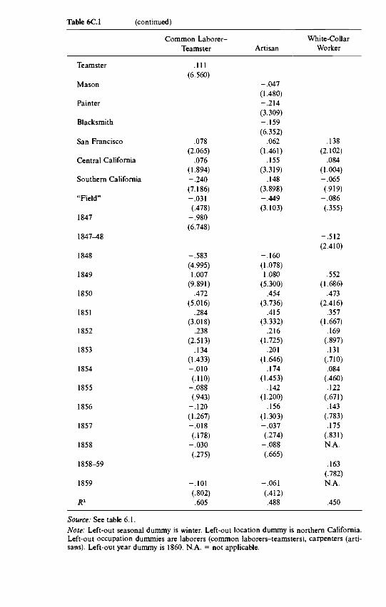
Table 6C.1 (continued)

Teamster

Mason

Painter

Blacksmith

San Francisco

Central California

Southern California

"Field"

1847

1847-48

1848

1849

1850

1851

1852

1853

1854

1855

1856

1857

1858

1858-59

1859

R2

Common Laborer-Teamster

.111(6.560)

.078(2.065)

.076(1.894)-.240(7.186)-.031(.478)

-.980(6.748)

-.583(4.995)1.007

(9.891).472

(5.016).284

(3.018).238

(2.513).134

(1.433)-.010(.110)

-.088(.943)

-.120(1.267)-.018(.178)

-.030(.275)

-.101(.802).605

Artisan

-.047(1.480)-.214(3.309)-.159(6.352)

.062(1.461)

.155(3.319)

.148(3.898)-.449(3.103)

-.160(1.078)1.080

(5.300).454

(3.736).415

(3.332).216

(1.725).201

(1.646).174

(1.453).142

(1.200).156

(1.303)-.037(.274)

-.088(.665)

-.061(.412).488

White-CollarWorker

.138(2.102)

.084(1.004)-.065(.919)

-.086(.355)

-.512(2.410)

.552(1.686)

.473(2.416)

.357(1.667)

.169(.897).131

(.710).084

(.460).122

(.671).143

(.783).175

(.831)N.A.

.163(.782)N.A.

.450

Source: See table 6.1.Note: Left-out seasonal dummy is winter. Left-out location dummy is northern California.Left-out occupation dummies are laborers (common laborers-teamsters), carpenters (arti-sans). Left-out year dummy is 1860. N.A. = not applicable.

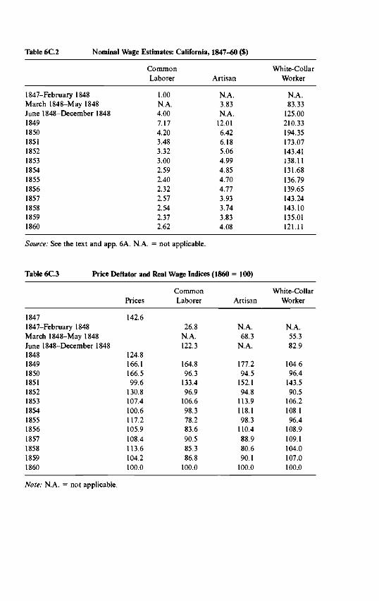
Table 6C.2 Nominal Wage Estimates: California, 1847-60 ($)

1847-February 1848March 1848-May 1848June 1848-December 1848184918501851185218531854185518561857185818591860

CommonLaborer

1.00N.A.4.007.174.203.483.323.002.592.402.322.572.542.372.62

Artisan

N.A.3.83N.A.

12.016.426.185.064.994.854.704.773.933.743.834.08

White-CollarWorker

N.A.83.33

125.00210.33194.35173.07143.41138.11131.68136.79139.65143.24143.10135.01121.11

Source: See the text and app. 6A. N.A. = not applicable.

Table 6C.3 Price Deflator and Real Wage Indices (1860

18471847-February 1848March 1848-May 1848June 1848-December 18481848184918501851185218531854185518561857185818591860

Prices

142.6

124.8166.1166.599.6

130.8107.4100.6117.2105.9108.4113.6104.2100.0

CommonLaborer

26.8N.A.122.3

164.896.3

133.496.9

106.698.378.283.690.585.386.8

100.0

= 100)

Artisan

N.A.68.3

N.A.

177.294.5

152.194.8

113.9118.198.3

110.488.980.690.1

100.0

White-CollarWorker

N.A.55.382.9

104.696.4

143.590.5

106.2108.196.4

108.9109.1104.0107.0100.0

Note: N.A. = not applicable.