SERC DISCUSSION PAPER 60

Wage Disparities in Britain: People orPlace?Stephen Gibbons (SERC, Department of Geography & Environment, LSEand CEP)Henry G. Overman (SERC, Department of Geography & Environment, LSEand CEP)Panu Pelkonen (SERC, Department of Geography & Environment, LSE andCEP)

October 2010

This work was part of the research programme of the independent UK Spatial Economics Research Centre funded by the Economic and Social Research Council (ESRC), Department for Business, Enterprise and Regulatory Reform (BERR), the Department for Communities and Local Government (CLG), and the Welsh Assembly Government. The support of the funders is acknowledged. The views expressed are those of the authors and do not represent the views of the funders. © S. Gibbons, H. G. Overman and P. Pelkonen, submitted 2010

Wage Disparities in Britain: People or Place?

Stephen Gibbons* Henry G. Overman**

Panu Pelkonen***

October 2010 * SERC, Department of Geography & Environment, London School of Economics ** SERC, Department of Geography & Environment, London School of Economics *** SERC, Department of Geography & Environment, London School of Economics Acknowledgements This work contains statistical data from ONS which is Crown copyright and reproduced with the permission of the controller of HMSO and Queen's Printer for Scotland. The use of the ONS statistical data in this work does not imply the endorsement of the ONS in relation to the interpretation or analysis of the statistical data. This work uses research datasets which may not exactly reproduce National Statistics aggregates. Copyright of the statistical results may not be assigned, and publishers of this data must have or obtain a licence from HMSO. The ONS data in these results are covered by the terms of the standard HMSO "click-use" licence.

Abstract This paper investigates wage disparities across sub-national labour markets in Britain using a newly available microdata set. The findings show that wage disparity across areas is very persistent over time. While area effects play a role in this wage disparity, most of it is due to individual characteristics (sorting). Area effects contribute a very small percentage to the overall variation of wages and so are not very important for understanding overall levels of wage disparity. Specifically, in our preferred specification area effects explain less than 1% of overall wage variation. This share has remained roughly constant over the period 1998-2008. Keywords: wage, disparities, labour JEL Classifications: R11, J31

1

1 Introduction

Places throughout the UK - regions, cities and neighbourhoods - appear very unequal. This is true if

we look at average earnings, employment, and many other socio-economic outcomes. Take Gross-

Value-Added per person, potentially a good indicator of income.2 In 2005, the highest ranked

(NUTS 3) regions in the UK were West Inner London and Berkshire with GVAs of £44050 and

£39850 respectively. The lowest ranked were Liverpool and Blackpool, with GVAs of £19800 and

£21050. These examples are representative of a broader trend – the top ranked 10% of UK (NUTS

3) regions have GVA at least 50% higher than the bottom ranked 10%.

Spatial policy at all scales is largely based around concerns about such disparities. But these figures

are simply aggregates of the outcomes for people who live and work in these places. Without

further analysis, we do not know whether outcomes for people working in London would be any

different if they worked in Liverpool. We do not know if the productivity of London and Liverpool

would change if these movements of people happened. Similarly, we do not know whether

replicating the economic, policy, and institutional regime of London in Liverpool would change

anything without moving people. In short, while it is (relatively) easy to measure aggregate

differences between places, it is much harder to work out what these differences mean in terms of

the advantages and disadvantages a place offers to people who live and work there.

Looking at these aggregated figures for areas, it is tempting to conclude that disparities between

places are big drivers of individual disparities. But this need not be the case. The differences

between people living and working within the same local area could far exceed the differences

between areas. Knowing whether 'between-area' or 'within-area' disparities dominate is thus

important in understanding the role policy might play in helping address individual disparities.

In this paper we present evidence on the nature, scale and evolution of economic disparities in

Britain, keeping these considerations of the relative contribution of people and place to the fore. We

focus on wages because wages are linked to productivity and variation in wages is an important

cause of variation in income. We also have good individual level (micro) data on wages. Using this

2 We estimate GVA per employee for NUTS 3 areas by dividing GVA by workplace-based employment. We then multiply GVA per employee by the working-age employment rate amongst residents in each NUTS 3 area. Employment-adjusted GVA per employee is thus indicative of expected GVA for a working age resident in a NUTS 3 area, assuming they could work in the same jobs as existing employees and have the same employment probability as existing residents. The employment numbers come from the Annual Business Inquiry via nomis (nomisweb.co.uk). GVA come from the ONS Sub-regional GVA release (ONS 2008). We present GVA figures rounded to the nearest £50.

2

micro data on workers' wages, linked to their place of work, we examine wage disparities across

labour market areas. We assess to what extent these disparities arise because of differences in the

types of workers in different areas (sorting) versus different outcomes for the same types of workers

in different areas (area effects). We then examine the extent to which these area differences

contribute to overall wage disparities. Our evidence provides a first step in answering questions

about the likely effectiveness of ‘people’-based policy directed at similar people in different places

as against ‘place-based’ policy directed at specific places in addressing overall disparities.

Our findings show that wage disparity across areas is very persistent. While most of this wage

disparity across areas is due to individual characteristics (sorting), area effects also play a role.

Specifically, in our preferred specification, sorting accounts for around 90% of the disparity

between places, while area effects account for around 10%. Area effects play an even smaller role

in understanding overall levels of individual wage disparity. In our preferred specification area

effects explain less than 1% of overall wage variation. The share accounted for by area effects has

remained fairly constant over the period 1998-2008.

Our paper is related to several literatures. Labour economists have long been concerned with the

role sorting on individual characteristics might play in explaining differences in wages between

groups of workers (particularly wage differences across industries). See, for example, Krueger and

Summers (1988), Gibbons and Katz (1992) and Abowd, Kramarz and Margolis. (1999). Sorting as

an explanation of spatial disparities has received less attention. Duranton and Monastiriotis (2002),

Taylor (2006) and Dickey (2007) use individual data to consider regional earnings inequalities in

the UK. Bell et al (2007) look at sub-regional wage differentials with a specific focus on the public

versus private sector.3 Relative to these papers we work with functional labour market areas (rather

than administrative boundaries) at a smaller spatial scale and, most importantly, we use panel data

to control for unobserved individual characteristics. A number of studies also use individual data to

study spatial sorting and agglomeration economies. See, for example, Mion and Natticchioni

(2009), Dalmazzo and Blasio (2007) and Combes, Duranton and Gobillon (2008). This paper is

most closely related to the last of these in terms of its overall approach and use of individual data.

However, whereas that paper is predominantly interested in the importance of skills, endowments or

3 There is also a large literature using data for areas, rather than individuals, which controls for structural characteristics

of the regions when considering, for example, spatial disparities in earnings or productivity. See, for example, Rice,

Venables and Pattachini (2006).

3

interactions based explanations of area effects, we focus on the contribution of area effects to

overall wage disparity.

The rest of this paper is structured as follows. Section 2 describes the data. Section 3 describes the

evolution of area disparities in Britain. Section 4 outlines our methodology for separating out the

role of area effects and composition and considering the contribution of these two components to

overall wage disparities. Section 5 presents results, while section 6 offers some conclusions.

2 Data

Our analysis is based on the Annual Survey of Hours and Earnings (ASHE) and its predecessor the

New Earnings Survey (NES) and covers 1998-2008. ASHE/NES is constructed by the Office of

National Statistics (ONS) based on a 1% sample of employees on the Inland Revenue PAYE

register for February and April. ASHE provides information on individuals including their home

and work postcodes, while the NES provides similar data but only reports work postcodes. We

mainly focus on area differences with workers allocated according to their work postcode allowing

us to use the whole sample. The National Statistics Postcode Directory (NSPD) provides a map

from every postcode to higher-level geographic units (e.g. local authority, region, etc). We assign

individuals to Travel to Work Areas using each individual’s work postcode. Given the way TTWA

are constructed (so that 75% of the resident population also work within the same area) the work

TTWA will also be the home TTWA for the majority of workers.

NES/ASHE include information on occupation, industry, whether the job is private or public sector,

the workers age and gender and detailed information on earnings including base pay, overtime pay,

basic and overtime hours worked. We use basic hourly earnings as our measure of wages.

NES/ASHE do not provide data on education but information on occupation works as a fairly good

proxy for our purposes. NES/ASHE provide national sample weights but as we are focused on sub-

national (TTWA) data we do not use them in the results we report below.4

Our analysis divides Britain into 157 “labour market areas” of which 79 are single “urban” TTWA

and 78 are “rural areas” created by combining TTWA. We reached this classification in three steps:

a) we identified the primary urban TTWAs as TTWA centred around, or intersecting urban-

footprints with populations of 100,000 plus; b) we identified TTWA with an annual average

4 Using these weights makes little difference to our results and no difference to our broad conclusions.

4

NES/ASHE sample size greater than 200 as stand-alone non-primary-urban TTWA (e.g. Inverness);

and c) we grouped remaining TTWA (with sample sizes below 200) into contiguous units (e.g.

North Scotland). A full list of the resulting labour market areas along with their average wage is

provided in Table A5 in the appendix. The geographical area boundaries are shown in Appendix 3.

3 The evolution of labour market wage disparities

We start by considering the evolution of wage disparities over the period 1998-2008 for our 157

labour market areas. Table 1 provides summary statistics by year. We report the mean area wage

(Mean), the standard deviation across areas (SD), the minimum and maximum area wage (Min and

Max), the coefficient of variation (CV) and the variance of log wage (var(lnw)). Unsurprisingly, the

mean, minimum and maximum of nominal wages all rise monotonically across time. The standard

deviation also rises which is not surprising given the increase in mean wage. The coefficient of

variation controls for rising overall wages by dividing the standard deviation by the mean. The

variance of log wages provides an alternative measure of variation which is invariant with respect to

common growth rates across areas. The coefficient of variation shows that, during the period, wage

disparity between areas rose slightly before falling back to roughly its initial level. The variance of

log wages (which will forms the focus of our analysis) shows an identical pattern. That is, the

overall level of between area wage disparity has remained roughly constant during our study period.

Table 1: Summary statistics: mean hourly wages, 157 labour market areas, 1998-2008

Year Obs Mean SD Min Mean CV var (lnw)1998 157 7.60 0.74 6.30 10.58 0.10 0.00871999 157 8.00 0.80 6.31 11.10 0.10 0.00932000 157 8.35 0.86 6.91 11.57 0.10 0.00982001 157 8.83 0.96 7.46 12.39 0.11 0.01052002 157 9.16 1.01 7.43 12.98 0.11 0.01092003 157 9.53 1.04 7.86 13.57 0.11 0.01072004 157 9.77 1.07 7.86 13.90 0.11 0.01082005 157 10.06 0.99 7.97 14.36 0.10 0.00872006 157 10.46 1.03 8.88 14.76 0.10 0.00882007 157 10.77 1.11 9.04 15.44 0.10 0.00952008 157 11.12 1.14 9.06 15.92 0.10 0.0095

Notes: Authors own calculations using NES/ASHE. Of course, these measures of disparity cannot tell us anything about the degree of persistence in any

given area’s average wages across time. It is possible that the overall stability in between area wage

disparity masks large changes in the fortunes of particular areas. Perhaps unsurprisingly, Figure 1

shows this is not the case. For each of our 157 areas, the figure plots hourly wages in 1998 against

hourly wages in 2008 (data for all areas are provided in Table A5 of the appendix, while Table A6

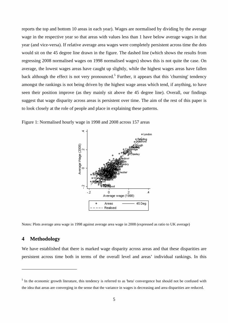
5

reports the top and bottom 10 areas in each year). Wages are normalised by dividing by the average

wage in the respective year so that areas with values less than 1 have below average wages in that

year (and vice-versa). If relative average area wages were completely persistent across time the dots

would sit on the 45 degree line drawn in the figure. The dashed line (which shows the results from

regressing 2008 normalised wages on 1998 normalised wages) shows this is not quite the case. On

average, the lowest wages areas have caught up slightly, while the highest wages areas have fallen

back although the effect is not very pronounced.5 Further, it appears that this 'churning' tendency

amongst the rankings is not being driven by the highest wage areas which tend, if anything, to have

seen their position improve (as they mainly sit above the 45 degree line). Overall, our findings

suggest that wage disparity across areas is persistent over time. The aim of the rest of this paper is

to look closely at the role of people and place in explaining these patterns.

Figure 1: Normalised hourly wage in 1998 and 2008 across 157 areas

Notes: Plots average area wage in 1998 against average area wage in 2008 (expressed as ratio to UK average)

4 Methodology

We have established that there is marked wage disparity across areas and that these disparities are

persistent across time both in terms of the overall level and areas’ individual rankings. In this

5 In the economic growth literature, this tendency is referred to as 'beta' convergence but should not be confused with

the idea that areas are converging in the sense that the variance in wages is decreasing and area disparities are reduced.

6

section, we outline our methods to consider the extent to which these area differences are driven by

area effects and the extent to which these, in turn, matter for individual outcomes. Our main focus

is: a) on the magnitude of these area effects and their contribution to overall wage disparities across

individuals, and b) the extent to which observed area differences arise because of differences in the

characteristics of workers who work in these areas (sorting of people) versus different outcomes for

the same workers living in different areas (area effects).

4.1 Wage regressions

Our empirical strategy is based on regression analysis of individual wages, which allows us to

estimate the magnitude of area effects, after allowing for differences in the characteristics of

workers in different areas. Imagine, for the moment, that all workers are identical and live in one of

J areas.6 Then allowing for area effects we can assume that wages are determined as:

'ln i i iw d (1)

where ln iw is the (natural logarithm of) wage of individual i, is a Jx1 vector of area effects, id is

a J x 1 vector or dummy variables that indicates in which of the J areas individual i works and iε is

an error term that represents unobserved wage factors that are uncorrelated with the area effects.

Estimating (1) by regressing individual (log) wages on a set of area dummy variables (using data

from 1998 and 2008) and plotting would give us a picture like Figure 1. Putting log wages on the

left hand side of (1) means that the component represents (approximately) the percentage

difference between the mean wage in a given area and the mean wage in some baseline area.

Of course, all workers are not identical. For example, those in higher-skill occupations, will get paid

more than those in low-skill occupations. We can capture the effect of both area and individual

characteristics by assuming that wages are determined as:

' 'ln i i i iw x d (2)

where ix is a vector of individual variables measuring skills, gender, age and other characteristics,

is a vector of coefficients that capture the “returns” to different individual characteristics and

everything else is as before. Now captures the impact of area controlling for the observed

6 Alternatively, assume workers differ but are randomly assigned to different places.

7

characteristics of individuals. That is they capture area effects once we control for the fact that

people with different characteristics get paid different wages and may work in different areas.

Likewise captures the impact of individual characteristics controlling for area.

These regressions identify area effects allowing for the possibility that workers with different

characteristics sort across areas providing that we have data available on all individual

characteristics that affect wage.7 Unless we have very rich data on individuals there is always the

possibility that sorting on some unobserved characteristic of individuals might drive the differences

in wages across areas and that the area dummies capture the effect of this sorting rather than the

causal effect of working in a particular area. Unfortunately, even with detailed data, we cannot be

certain that we are observing everything that might affect wages. For example, in our data we have

no information on education, cognitive abilities or motivation. So when we compare people with

identical observed characteristics it may be that those with higher education or ability live in a

particular area. Assuming workers with higher education or ability get paid more, it is the

unobserved individual characteristics (education and ability) that explain the higher wage of the

individuals living in the area but we mistakenly attribute it to an effect of the area.

One solution is to follow the same individual as they move across areas. Providing that unobserved

characteristics are fixed over time, if the same individual earns more in some areas than others we

can be more confident in attributing this to an area effect rather than a composition (sorting) effect.

Even then, we cannot rule out the possibility that something changed for the individual that both

affected their wage and their place to work. In the absence of random allocation (or a policy change

that as good as randomly assigns people) tracking individuals and observing the change in wages

experienced when they move between areas is the best we can do to identify true area effects.

Formally, we use the panel dimension of NES/ASHE to include fixed effects for each individual i:

' 'ln i i t i i iw x d (3)

where the i are individual fixed effects (that capture the effect of unobserved time invariant

characteristics such as ability) and the t are time dummies that pick up the fact that average wages

7 More precisely we need data on all individual characteristics that are correlated with the area effects.

8

change over time.8 The need to pool data across time to control for unobserved individual

characteristics comes at a cost – sample size restrictions mean we can no longer consider year on

year changes in the area specific effects.9 As we shall see, however, these area specific effects

appear to be quite stable over time, while individual unobserved characteristics are, unsurprisingly,

important for explaining wage. So there are good reasons to think that the panel regression which

assumes area effects are fixed but allow us to include individual fixed effects may give the most

accurate picture of the relative roles of composition versus area effects.

Once we have estimated these area effects we can use the distribution across areas to describe the

impact on an individual of moving from a “bad place” (in terms of wages) to a “good place”. We

can also describe how this distribution of area effects changes as we include observed individual

characteristics and individual fixed effects in the wage regressions. This provides a first indication

of the extent to which observed area disparities are due to sorting versus area effects. To provide a

more formal assessment we use several related variance decompositions to assess the contribution

of area effects to area disparities and to overall wage disparities. These decompositions allow for

the fact that the contribution to overall wage disparities depends not only on the size of specific

effects but also on the overall distribution of good and bad places and on the distribution of

individuals across those places. Variance decompositions summarise this interaction, while also

providing a more rigorous assessment of the extent to which sorting contributes to observed area

wage disparities.

4.2 Analysis of Variance

For simplicity, consider the wage regressions for one year where we are only worried about

controlling for observed individual characteristics such as age, gender and skills (vector ix ):

' 'ln i i i iw x d (4)

where everything is defined as above. We want to find the contribution of area effects to area

disparities and to the total variance of (log) wages. We focus on deriving the contribution of area

8 Note that we did not need to include these time dummies before because, when we do not include fixed effects, we can

run the regressions year by year.

9 Theoretically, we could still allow for such year on year changes in place specific effects, but identifying them

requires movers in and out of all areas in every year which turns out to be too demanding given our sample sizes.

9

effects to overall wage disparities and use this to back out the contribution of area effects to area

disparities. There are, however, two ways to conceptualise and measure the contribution to overall

wage disparities. The first is to estimate the ratio '( ) / (ln )i iVar d Var w whilst allowing to be

correlated with individual characteristics ix .10 The second is to estimate the ratio

( ) / (ln )iVar u Var w where we consider only u the components of that are uncorrelated with ix .

We now explain this in more detail.

Suppose we ignore the differences between individuals and run the regression of log wage on a set

of area dummy variables to estimate the area effects 'id . The R-squared from this regression,

2 ' ˆ(ln ; )i iR w d , captures the proportion of total variance in wages explained by area including both

the effects of sorting and area effects. This is because the R-squared is ' ˆ( ) / (ln )i iVar d Var w where

are the estimated area effects (i.e. the coefficients on the area dummy variables). Assuming that

sorting is ‘positive’ or (so individuals with high wage characteristics tend to move to high wage

places) then this provides an upper bound for the contribution of area effects (because some of the

difference between areas is due to sorting but we attribute it all to area effects).

To include individual characteristics, regress log wage on ix and area dummies id . Next, predict the

components of wages due to characteristics ( ˆix ) and area effects ( 'id ) and note that:

ˆ ˆ ˆln

ˆ ˆ ˆ ˆ ˆ2 ,

i i i i

i i i i i

Var w Var x d

Var x Var d Cov x d Var

(5)

where we ignore the covariance terms between the residual ( ) and ix and 'id because they are

uncorrelated by construction.11 As before, we can obtain a measure of the contribution of area

effects as ' ˆ( ) / (ln )i iVar d Var w . This measure is smaller than the R-squared without any covariates

ix , because that measure attributed all of the covariance between ix and 'id to area effects. Notice

that there is no reason why the estimated area effects should be uncorrelated with the individual

10 Note the variance )(Var is the variance over the sample of individual workers, not areas

11 This statement holds for the estimated residuals even if these components are correlated with the true error term.

10

characteristics ix , but that the initial regression does control for the fact that individuals with

different ix earn different wages and may live in different areas when estimating . This means

that ' ˆ( ) / (ln )i iVar d Var w excludes the direct contribution of sorting (i.e. the covariance term in

equation (5)), but captures any indirect effect that sorting may have on the variance of the area

effects. That is, it captures the contribution of area effects including those induced by composition

(e.g. spillovers and interactions) but not the effects, if any, that area has in determining individual

characteristics. We refer to this as the correlated area variance-share, because the estimated area

effects are potentially correlated with individual characteristics. Because the correlated variance-

share excludes the direct contribution of sorting it can also be used to calculate the contribution of

area effects to area disparities. To do this we simply take the ratio of the correlated area variance

share (which excludes sorting) to the proportion of total variance in wages explained by area

including both the effects of sorting and area effects. That is, we take the ratio of the correlated

variance share to 2 ' ˆ(ln ; )i iR w d that we get by estimating area effects from a regression of log

wages on only a set of area dummy variables.

We can also estimate the contribution of the components of area effects that are uncorrelated with

individual characteristics. There are a number of equivalent methods for doing this that give a

statistic that is usually called the semi-partial R-squared. One way is to first regress log wage on

observed individual characteristics ix and area dummies and obtain the R-squared based on the

estimated coefficients, 2 'ˆ ˆ(ln ; , )i i iR w x d . This measures the proportion of the overall variance

explained by both individual characteristics and area effects. Next, regress log wage on just the

observed individual characteristics and take the R-squared 2 ˆ(ln ; )i iR w x . This gives the proportion

of the overall variance explained by just the individual characteristics. The semi-partial R-squared is

the difference between the two 2 'ˆ ˆ(ln ; , )i i iR w x d – 2 ˆ(ln ; )i iR w x . Note, that if we do not include ix

in the regression, we just have the simple R-squared, 2 ' ˆ(ln ; )i iR w d , which is the same as that

produced by the variance-share method without any individual control variables. Another approach

is based on partitioned regression and starts by regressing log wage on ix and area dummies, and

obtaining the predicted values ˆix and 'id . Next regress 'id on ˆ

ix and get the uncorrelated

residual area components iu . Finally, regress log wage on the residual iu and look at the R-squared

(or square the partial correlation between log wage and the residual). Appendix 5 shows that these

methods are equivalent. In practise, the semi-partial R-squared can also be obtained using Analysis

11

of Variance (ANOVA), by dividing the partial sum of squares for the area effects 'id by the total

sum of squares.

The semi-partial R-squared can be estimated by all these methods, and in this context we refer to it

as the uncorrelated area variance-share. This is because it shows the amount of variation in log

wage that is explained by the part of the area effect that is uncorrelated with individual

characteristics (those that are included in ix ). That is, it captures the contribution of the components

of area effects that are uncorrelated with individual characteristics. This variance share will be

smaller than the correlated area variance-share described above (see Appendix 5) and may

understate the contribution of area effects if sorting has indirect effect on area effects or if areas

induce changes in the observed individual characteristics. Again, because the uncorrelated variance

share excludes both the direct and indirect contribution of sorting it can be used to calculate another

measure of the contribution of area effects to area disparities. As with the correlated variance share,

to do this we simply take the ratio of the uncorrelated area variance share (which excludes the direct

and indirect contribution of sorting) to the proportion of total variance in wages explained by area

including both the effects of sorting and area effects.

To recap, the correlated area variance-share (when controlling for ix ) shows the contribution of

the area effects after controlling for sorting. However, it includes the contribution of area effects

that arise because of that sorting, for example as a result of interactions between area effects and

individual characteristics, or because of spillovers to an individual from the average worker

characteristics in an area. The uncorrelated area variance-share (when controlling for ix ) captures

only the contribution of area effects that are uncorrelated with individual characteristics. It thus nets

out any benefits an individual gets from an area because of the composition of the labour force in

that area, for example any benefits from being located in an area with more high-skill workers.

To summarise, it is useful to consider an example. Suppose some areas have a better climate than

others, but are otherwise identical, and that a better climate makes people more productive. Imagine

that a) a better climate also attracts more high-skill workers such that places with a good climate

also have higher than average skills or b) a better climate encourages workers to acquire more

skills. In these cases the places with the better climate also have a high skilled workforce, but the

area effect on individual productivity that we are interested in is caused only by the climate. In this

case the 'upper bound' estimate of the contribution of area effects is obtained by

2 ' ˆ(ln ; )i iR w d ,where is estimated from a regression without any controls for worker skills, and

12

captures the effect of climate and the impact on area disparities from the sorting of high skill

workers. If instead, is estimated from a regression with controls for skills, then both the

correlated variance share ' ˆ( ) / (ln )i iVar d Var w and the uncorrelated variance share

2 'ˆ ˆ(ln ; , )i i iR w x d – 2 ˆ(ln ; )i iR w x yield an upper bound estimate of the contribution of area

differences in climate to individual disparities, purged of any additional area disparities caused by

sorting.

Suppose in addition, that working in an area amongst high skill workers makes individuals more

productive. In this case the correlated variance share will pick up this area effect in addition to the

direct effect from the climate. The uncorrelated variance share on the other hand will be an area

contribution to individual wage disparity that is purged of this contribution to individual wages that

acts from climate, via the average skill level in the area, and purged of any other components of

climate that are correlated with skills (e.g. through sorting). The uncorrelated variance share is thus

a lower bound to the contribution of area effects.

5 Results

5.1 All areas

We start by estimating equations 1, 2 and 3 to show how allowing for sorting across areas affects

the magnitude of estimated area effects. To summarise the distribution of effects we report the

percentage change in wages when we move between different parts of the distribution: the

minimum to maximum and to mean, mean to maximum, the 10th to the 90th percentile and the 25th

to the 75th percentile. Table 2 reports results based on several different specifications. The first row

reports results from equation (1) when only including time dummies giving the upper bound

estimates of area effects as discussed above. The second row reports results from equation (2) when

the observable variables are a set of age dummies, a gender dummy and a set of 1 digit occupation

dummies. The third row uses a set of age dummies, a gender dummy, two digit occupations

dummies, industrial dummies (three digit SIC) and dummies for public sector workers, part time

workers and whether the worker is part of a collective agreement. Results from equation (3) using

individual fixed effects are reported in rows four and five. In row four, we simply include year

dummies and individual effects. Row five uses individual effects, year dummies, age dummies and

13

one digit occupation dummies. The coefficients from one of these specifications (set of age

dummies, a gender dummy and a set of 1 digit occupation dummies) are reported in Appendix 4.12

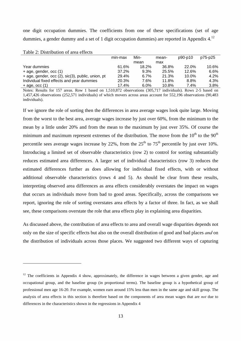
Table 2: Distribution of area effects min-max Min-

mean mean-max

p90-p10 p75-p25

Year dummies 61.6% 18.2% 36.8% 22.0% 10.6%+ age, gender, occ (1) 37.2% 9.3% 25.5% 12.6% 6.6%+ age, gender, occ (2), sic(3), public, union, pt 29.4% 6.7% 21.3% 10.0% 4.2%Individual fixed effects and year dummies 20.3% 7.6% 11.8% 8.8% 4.3%+ age, occ (1) 17.4% 6.0% 10.8% 7.4% 3.8%Notes: Results for 157 areas. Row 1 based on 1,510,872 observations (305,717 individuals). Rows 2-5 based on 1,457,426 observations (252,571 individuals) of which movers across areas account for 552,196 observations (90,483 individuals). If we ignore the role of sorting then the differences in area average wages look quite large. Moving

from the worst to the best area, average wages increase by just over 60%, from the minimum to the

mean by a little under 20% and from the mean to the maximum by just over 35%. Of course the

minimum and maximum represent extremes of the distribution. The move from the 10th to the 90th

percentile sees average wages increase by 22%, from the 25th to 75th percentile by just over 10%.

Introducing a limited set of observable characteristics (row 2) to control for sorting substantially

reduces estimated area differences. A larger set of individual characteristics (row 3) reduces the

estimated differences further as does allowing for individual fixed effects, with or without

additional observable characteristics (rows 4 and 5). As should be clear from these results,

interpreting observed area differences as area effects considerably overstates the impact on wages

that occurs as individuals move from bad to good areas. Specifically, across the comparisons we

report, ignoring the role of sorting overstates area effects by a factor of three. In fact, as we shall

see, these comparisons overstate the role that area effects play in explaining area disparities.

As discussed above, the contribution of area effects to area and overall wage disparities depends not

only on the size of specific effects but also on the overall distribution of good and bad places and on

the distribution of individuals across those places. We suggested two different ways of capturing

12 The coefficients in Appendix 4 show, approximately, the difference in wages between a given gender, age and

occupational group, and the baseline group (in proportional terms). The baseline group is a hypothetical group of

professional men age 16-20. For example, women earn around 15% less than men in the same age and skill group. The

analysis of area effects in this section is therefore based on the components of area mean wages that are not due to

differences in the characteristics shown in the regressions in Appendix 4

14

these contributions by considering the correlated and uncorrelated area variance-shares of estimated

area effects, controlling for individual characteristics.

Table 3 reports results for the contribution of area differences to area and overall wage disparities

using these two different measures. We calculate them from regression specifications using the

same individual characteristics as in Table 2. To recap, the first specification includes only time

dummies, the second dummies for gender, age and 1 digit occupation, the third additional job

characteristics and a fuller set of occupation and industry dummies, the fourth individual fixed

effects and the fourth individual fixed effects, age and one digit occupation dummies. For

comparison, the second part of the table reports the contribution of the individual characteristics

using the two different measures. The third part reports the contribution of area effects to area

disparities calculated by taking the ratio of the correlated and uncorrelated variance shares to the

variance share with area and year effects only (i.e. that reported in the first column).

Table 3: Variance decomposition

Year dummies only

+ age, gender, occ (1)

+ age, gender, occ (2), sic(3), public, union, pt

Individual fixed effects and year dummies

+ age, occ (1)

Area variance share Correlated with X 5.96% 2.88% 2.08% 0.75% 0.62%Uncorrelated with X 5.96% 2.73% 1.51% 0.08% 0.06%Individual variance share Correlated with area - 58.2% 76.0% 86.4% 87.9%Uncorrelated with area - 55.0% 71.6% 83.7% 84.9%Area share of area disparities Correlated with X 48.4% 35.1% 12.6% 10.4%Uncorrelated with X 46.8% 25.4% 1.3% 1.0%Notes: Column 1 based on 1,510,872 observations (305,717 individuals). Columns 2-5 based on 1,457,426 observations (252,571 individuals) of which movers across areas account for 552,196 observations (90,483 individuals). Even if we ignore the effects of sorting, and simply consider raw area differences in mean log

wages, the first column of Table 3 shows that these only explain 6% of the overall variation in

wages (remember that if we don't control for any Xs then the variance share of area effects is the

same whichever we calculate it). The contribution of area effects is less than 3% once we control

for basic observable characteristics (columns 1 and 2) and less than 1% once we control for

unobservable individual characteristics. In short, area effects only play a small role in explaining

overall wage disparities. The final part of the table shows that they play a somewhat more important

role in explaining area disparities. When we only account for basic characteristics, sorting accounts

for a little over half of the observed area disparities leaving area effects to account for around 48%.

15

Once we control for individual fixed effects the upper bound estimate of the contribution of area

effects to area disparities is considerably smaller at a little over 10% with the lower bound estimate

around 1%.

As discussed in Section 4.2, the correlated variance share provides an upper bound to the combined

contribution of exogenous area effects plus interactions-based spillovers. The uncorrelated variance

share provides a lower bound to the contribution of exogenous area effects alone. Looking at the

gap between these lower and upper bounds reveals that area effects arising from interactions-based

spillovers cannot account for much of the individual disparity in wages - between 0.56 and 1.2%.

This is however, quite substantial part of the overall contribution of area effects, accounting for

nearly all of it in the last column.

In contrast to these results on area effects, the contribution of individual characteristics is large.

Age, gender and occupation variables alone account for 55-58% of the individual disparity in

wages. Adding in individual fixed effects drives this share up to between 85% and 88% in the last

column, implying that the contribution of individual characteristics is over 140 times bigger than

that of area effects.

Table 4 shows that this contribution has been stable over time. For each year, the table reports the

contribution of raw area disparities (column 1) and the correlated (column 2) and uncorrelated

(column 3) area variance shares controlling for the fullest possible set of individual characteristics.

For comparison, the first row reports results when pooling across years (taken from table 3).

Repeating other results from table 3 by year (or by three year pools for the individual fixed effects

specifications) give figures that are similarly stable across years. Given this stability over time, we

tend to focus on the results for data pooled across years in the remainder of the paper.

16

Table 4: Area effects: Results by year

Year dummies only

+ age, gender, occ (2), sic(3), public, union, pt correlated x

+ age, gender, occ (2), sic(3), public, union, pt uncorrelated x

Pooled 5.96% 2.08% 1.51%1998 6.15% 2.05% 1.08%1999 6.03% 1.95% 1.04%2000 6.00% 1.99% 1.06%2001 6.34% 2.07% 1.11%2002 6.56% 2.32% 1.24%2003 6.60% 2.35% 1.27%2004 6.65% 2.32% 1.26%2005 6.53% 2.11% 1.17%2006 6.23% 2.07% 1.15%2007 6.78% 2.06% 1.12%2008 6.67% 2.10% 1.14%Notes: Column 1 based on 1,510,872 observations (305,717 individuals). Columns 2 and 3 based on 1,457,426 observations (252,571 individuals) of which movers across areas account for 552,196 observations (90,483 individuals). Contribution for pooled lower than average of years because pooled regressions impose time invariant area effects and coefficients on individual characteristics.

We have suggested that observed area differences overstate the contribution of area effects because

they conflate the effect of place with sorting across place on the basis of individual characteristics.

Figures 2-4 demonstrate this sorting process. Each figure graphs normalised area effects against

normalised area averages for predicted wages on the basis of observable individual characteristics

(figure 2), unobservable individual characteristics (figure 3) and both the sum of observable and

unobservable individual characteristics (figure 4). That is, in the notation of equations (3) and (4),

the figures plot normalised against normalised x (figure 2), (figure 3) and ˆˆ x (figure

4) where hats designate estimated coefficients and means are taken for all individuals in each area.

17

Figure 2: Area effects against observed individual characteristics

Notes: Plots area effects against average area predicted wage based on observed individual characteristics from a regression that includes individual fixed effects and observed individual characteristics (set of age dummies and a set of 1 digit occupation dummies)

Figure 3: Area effects against unobserved individual characteristics

Notes: Plots area effects against average area individual effects from a regression which includes individual fixed effects and observed individual characteristics (set of age dummies, and a set of 1 digit occupation dummies)

18

Figure 4: Area effects against observed and unobserved individual characteristics

Notes: Plots area effects against average area predicted wage based on both individual fixed effects and observed individual characteristics (set of age dummies, a gender dummy and a set of 1 digit occupation dummies) We have shown in figure 1 that observed spatial disparities are highly stable over time in the sense

that places at the top have tended to stay at the top, and places at the bottom have tended to stay at

the bottom. Figure 5 shows that this stability is not quite as pronounced for area effects.

Figure 5: Normalised area effects in 1998 and 2008 across 157 areas

Notes: Plots area effects from 1998 against area effects in 2008, based on regressions of wage on area dummies and observed individual characteristics (set of age dummies, a gender dummy, a set of 3 digit occupation dummies, 2 digit sector dummies and dummies for whether worker is part-time, public sector and subject to collective wage bargaining)

19

Once again, the 45 degree line shows what would have happened if there were no changes in the

distribution of area effects, while the dashed line reports a regression line showing what actually

happened. We see that, as for the overall area means, there is some churning, but the patterns are

quite stable. Once again, this stability is particularly pronounced for those areas at the upper end of

the area effects distribution. Further detail is provided in Table A7 in the appendix which reports

the figures for the top and bottom 10 area effects in 1998 and 2008.

Before moving on, note that Figure 5 is quite reassuring for our specifications where we control for

individual fixed effects. To do this, we need to assume that area based effects are fixed over time.

Of course, checking this in an internally consistent manner is impossible given that we have to

impose the assumption of stability to allow for the introduction of fixed effects to control for

unobserved individual effects. Still, it is reassuring that area based effects identified by controlling

only for observable individual characteristics were quite stable over time.

Overall, our findings so far suggest that area effects do not play a very important role in explaining

the difference in wages across areas but that positive correlation between area effects and individual

effects reinforce the effect that each has individually on overall wage inequality.

5.2 Urban versus Rural Areas

Our analysis so far has been based on 157 areas which represent both urban TTWA and

aggregations of rural TTWA. This section examines the differences between those urban and rural

areas as well as considering whether there are rural-urban differences within each of the TTWAs.

We start in figure 6, by replicating figure 1 showing the relationship between observed area average

wages in 1998 and 2008 but with the samples now split in to urban and rural areas.

Several things are apparent from the figures. First, unsurprisingly, the places with the highest

average wages are urban areas, while the places with the lowest average areas are rural (to see this

take a look at the minimum and maximums of the axis). Second, the distribution of rural averages is

slightly narrower than the distribution of the urban averages and there is substantial overlap

between the two sets of areas in terms of average wages. Third, there has been more change in the

rankings of rural areas (the regression line is below the 45 degree line) and almost no change on the

rankings in urban areas (which lies on the 45 degree line).

20

Figure 6: Normalised area wages in 1998 and 2008 for urban (top) and rural (bottom) areas

Notes: Plots average area wage in 1998 against average area wage in 2008 (expressed as ratio to UK average) for 79 urban areas (top panel) and 78 rural areas (bottom panel)

Not only has there been slightly more movement in the rankings of areas within the rural group, but

rural areas have also slightly improved their average position with respect to urban areas. The

summary statistics make this clearer. Table 5 reports observed area averages over time for the urban

and rural group as well as the average percentage urban-premium. In 1998 average area wages for

21

the urban group where £7.87 per hour, 7.4% above average wages for the rural group of £7.33 per

hour. By 2008 the percentage difference in area averages had fallen to 6.5%.

Table 5: Mean area wages for rural and urban areas Urban Rural urban premium

1998 7.87 7.33 7.4% 1999 8.29 7.70 7.7% 2000 8.65 8.04 7.6% 2001 9.16 8.49 7.8% 2002 9.54 8.78 8.6% 2003 9.91 9.15 8.3% 2004 10.11 9.43 7.2% 2005 10.40 9.72 7.0% 2006 10.79 10.13 6.5% 2007 11.13 10.41 6.9% 2008 11.46 10.77 6.5%

Notes: Column 1 reports average wage for 79 urban areas, column 2 average wage for 78 rural areas. Column 3 reports average percentage urban-premium

As with our earlier analysis we would like to distinguish between the role of area effects and that of

composition or sorting on individual characteristics. To do this we again run regressions based on

equations (1)-(3) above. We do this separately for the rural and urban samples to allow the effects

of individual characteristics ix on log wages to be different in the rural and urban areas (the

regression coefficients are shown in Appendix 4). Table 6 replicates results in table 2 on the

distribution of area effects for the two different samples of rural and urban areas

Table 6: Distribution of area effects for rural and urban areas

Min-max

Min-mean

mean-max

p90-p10

p75-p25

Urban-rural1

Urban Year dummies 51.3% 14.2% 32.6% 26.1% 10.9% 6.5%+ age, gender, occ (1) 33.1% 8.4% 22.8% 13.6% 6.4% 4.2%+ age, gender, occ (2), sic(3), public, union, pt 28.3% 7.5% 19.3% 11.6% 5.3% 2.9%Individual fixed effects and year dummies 18.0% 7.4% 9.9% 6.3% 3.3% 2.8%+ age, occ (1) 14.8% 5.3% 9.0% 5.8% 3.1% 2.4%Rural Year dummies 47.6% 14.5% 28.9% 20.0% 8.0% + age, gender, occ (1) 27.9% 7.4% 19.1% 12.6% 5.2% + age, gender, occ (2), sic(3), public, union, pt 20.1% 5.2% 14.2% 7.6% 3.6% Individual fixed effects and year dummies 20.3% 6.8% 12.7% 10.0% 5.6% + age, occ (1) 18.1% 6.6% 10.7% 8.4% 5.4% Notes: Results for 79 urban and 78 rural areas. Urban results based on 1,208,698 observations (260,240 individuals). Rural results based on 302174 observations (75,717 individuals). Last columns reports the difference between the mean urban area effect and the mean rural area effect. The effect of sorting between urban and rural areas is immediately apparent from the final column.

Starting from a raw urban-rural area premium of 6.5% the premium reduces markedly to 2.4% once

we control for observed and unobserved individual characteristics. With the exception of min to

22

mean, the table shows greater spread in the raw observable differences between urban areas relative

to rural areas. The picture is mixed once we control for individual characteristics. The extremes of

the urban distribution are more pronounced, but the rural distribution shows slightly more

dispersion across the 90-10 and the 75-25 percentiles.

Once again, we use variance decompositions for the two different samples to make more precise

statements about the relative importance of area effects. Results are reported in table 7 and should

be compared to those in table 3. When we ignore the role of sorting, area effects explain 5.7% of the

variance of wages for individuals working in urban areas, almost twice as much as for those

working in rural areas. Initially, this difference (i.e. that areas account for more of the variance of

urban wages) persists when controlling for individual characteristics. Area effects explain less than

1% of rural wage disparities when we control for basic individual characteristics (second column),

while continuing to explain about 2.5% of urban disparities. Interestingly, this difference disappears

once we control for unobserved individual characteristics. Turning to the contribution of area

effects to area disparities we see that when we control for basic observable characteristics the

importance of sorting is roughly similar across the two types of areas leaving area effects to explain

slightly less than half of observed area disparities. Controlling for individual fixed effects the share

of area effects in area disparities decreases more for urban than for rural areas. Overall, these

differences suggest two things. First, sorting is more pronounced across urban than rural areas

(which explains why, for urban areas, there is a greater difference between the role of observed area

effects and that of area effects once we control for sorting). Second, the fact that individual

unobservables play a larger role in reducing the contribution of area effects for urban areas,

suggests that sorting on unobservables must be more important for urban than for rural areas.

Figures 7-9 show that this is indeed the case.

Table 7: Variance decomposition in urban and rural areas

Year dummies only

+ age, gender, occ (1)

+ age, gender, occ (2), sic(3), public, union, pt

Individual fixed effects and year dummies

+ age, occ (1)

Urban Area variance share Correlated with X 5.71% 2.70% 2.07% 0.63% 0.52%Uncorrelated with X 5.71% 2.78% 1.47% 0.06% 0.06%Area share of area disparities Correlated with X 47.3% 36.3% 11.0% 9.1%Uncorrelated with X 48.7% 25.7% 1.1% 1.1%Rural Correlated with X 2.39% 0.99% 0.54% 0.61% 0.51%Uncorrelated with X 2.39% 0.97% 0.29% 0.02% 0.02%

23

Area share of area disparities Correlated with X 41.4% 22.6% 25.5% 21.3%Uncorrelated with X 40.6% 12.1% 0.8% 0.8%Notes: Results for 79 urban and 78 rural areas. Urban results based on 1,208,698 observations (260,240 individuals). Rural results based on 302174 observations (75,717 individuals). Figure 7 shows that sorting on observables occurs for both urban and rural areas (the positive slope)

but that positive association is less strong for the rural areas. Figure 8 shows that sorting on

unobservables is much more pronounced for urban than for rural areas. Indeed, for rural areas there

is almost no relationship between area effect and the (unobserved) individual effects while for urban

areas it is clearly positive. Finally Figure 9 shows the overall effect of sorting on both observable

and unobservable individual characteristics. As discussed above, sorting is stronger for urban than

for rural areas. This is consistent with the fact that areas account for more of the variance of urban

wages than of rural wages before we control for sorting (5.71% versus 2.39%) but that there is no

difference in the contribution of area effects to overall wage disparities once we control for sorting

(see the final column of Table 7).

Figure 7: Area effects against observed individual characteristics for urban (top panel) and rural (bottom panel) areas

24

Notes: Plots area effects against average area predicted wage based on observed individual characteristics from a regression that includes individual fixed effects and observed individual characteristics(of age dummies and a set of 1 digit occupation dummies ) for 79 urban areas (top panel) and 78 rural areas (bottom panel)

25

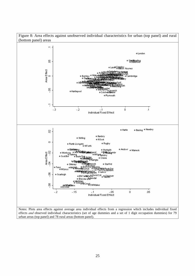
Figure 8: Area effects against unobserved individual characteristics for urban (top panel) and rural (bottom panel) areas

Notes: Plots area effects against average area individual effects from a regression which includes individual fixed effects and observed individual characteristics (set of age dummies and a set of 1 digit occupation dummies) for 79 urban areas (top panel) and 78 rural areas (bottom panel).

26

Figure 9: Area effects against observed and unobserved individual characteristics for urban (top panel) and rural (bottom panel) areas

Notes: Plots area effects against average area predicted wage based on both individual fixed effects and observed individual characteristics (set of age dummies and a set of 1 digit occupation dummies) for 79 urban areas (top panel) and 78 rural areas (bottom panel).

Finally, as for the overall sample, we can ask whether area effects are as stable as observed area

differences once we separate between rural and urban areas. Figure 10 shows that, as with observed

disparities, we have seen greater churn in area effects for rural than for urban areas.

27

Figure 10: Normalised area effects in 1998 and 2008 for urban (top panel) and rural (bottom panel) areas

Notes: Plots area effects from 1998 against area effects in 2008 for 79 urban areas (top panel) and 78 rural areas (bottom panel). Based on regressions of wage on area dummies and observed individual characteristics (set of age dummies, a gender dummy, a set of 3 digit occupation dummies, 2 digit sector dummies and dummies for whether worker is part-time, public sector and subject to collective wage bargaining)

28

5.3 Other issues

One obvious concern is that, for the specifications that include individual effects, identification

comes from movers, but the variance analysis is based on all individuals. Results reported in table 8

show what happens when the sample is restricted to movers only. Comparing to table 3 we see that

the upper bound estimate of area differences attributes less of the variation in wages (about 4%

compared to 6%) to area, but once we start controlling for individual differences we see similar

results with area effects explaining a small percentage of variation in wages. Two offsetting effects

could be at work here. First, the variance of log wages may be higher for movers than for the whole

sample so if estimated area effects were unchanged their contribution would necessarily be lower.

Offsetting this, we expect movers to either (i) be more affected by area differences (because they

move in response to those differences) or (ii) to be people who have experienced a shock to wages

that make them more likely to move. Both these effects would tend to increase the magnitude of

estimated area effects. In practise, these offsetting effects appear to be in play, but neither is large.

Table 8: Movers

Area variance share

Year dummies only

+ age, gender, occ (1)

+ age, gender, occ (2), sic(3), public, union, pt

Individual fixed effects and year dummies

+ age, occ (1)

Correlated with X 4.23% 2.01% 1.43% 0.67% 0.52%Uncorrelated with X 4.23% 1.96% 0.98% 0.22% 0.17%

Results based on 552859 observations (91146 individuals).

Another issue of possible concern is that our analysis is based on where individuals work, rather

than where they live. If areas were closed so that people did not commute across borders then this

would make no difference. But in a world where people do commute it is possible that home based

area effects play a more important role than work based area effects in explaining wage disparities.

In fact, a comparison of work and home-based areas (results not tabulated here) shows that these

differences are small. Aarea disparities are marginally bigger for work-based than home-based

areas, but the general patterns are the same as we observed in Table 3 above.

6 Conclusions

This paper assesses the extent and evolution of wage disparities across sub-national labour markets

in Britain using a newly available microdata set. The findings show that wage differences across

areas are very persistent. While some of this is due to individual characteristics (sorting), area

29

effects also play a role. However, area effects contribute a small percentage to area disparities and a

very small percentage to total variation in wages. That is, they are not very important for

understanding either area or overall wage disparity. Specifically, in our preferred specification area

effects contribute around 10% to area disparities and less than 1% of total wage variation. This

share remained roughly constant over the period 1998-2008.

These results need to be interpreted with caution. We note three main caveats. First, our estimates

remain an upper bound if unobserved time varying individual effects are correlated with area effects

because of their impact on moving decisions. Second, we do not study differences in the probability

of earning a wage (e.g. due to employment rate differences) or in other components of income.

Third, we do not control for differences in costs of living and in access to amenities across places.

In other words, we are studying nominal not real wages. These issues are important and we consider

them in a companion paper (Gibbons, Overman, Resende, 2010)

These caveats aside, we identify several important policy messages. First, area effects do not make

a large direct contribution to area disparities. Second, area affects are even less important in

understanding total wage disparities. Third, there is a positive correlation between area effects and

individual characteristics associated with higher wages. This means that these effects may play an

important role in shaping the economic geography of the UK because they (partly) drive sorting

which does play an important role in driving area disparities. Fourth, if we view spatial policy as a

means of addressing individual wage inequalities then identifying places with bad area effects may

help with targeting (due to the correlation between individual characteristics and area effects).

However, trying to address area effects directly will not have a large impact on total wage

disparities. If addressing total wage disparities is the primary policy objective (and we would argue

that it should be), then policy objectives expressed in terms of aggregate area outcomes may lead

policy to focus too strongly on area effects and on the spatial sorting of workers with different

characteristics. As a result policy may focus too little on addressing much more significant within-

area inequalities.

7 References

Abowd, J., F. Kramarz and D. Margolis. (1999). “High Wage Workers and High Wage Firms,”

Econometrica, 67(2), 251-333.

30

Borcard (2002). “Multiple and partial regression and correlation: Partial r2, contribution and

fraction [a].” Processed Université de Montréal.

http://biol09.biol.umontreal.ca/borcardd/partialr2.pdf (Accessed 31/08/2010)

Bell, D., R.F. Elliott, A. Ma, A. Scott, and E.Roberts (2007). "The Pattern and Evolution of

Geographical Wage Differentials in the Public and Private Sectors in Great Britain," The

Manchester School, 75(4), 386-421

Combes, P.P, G. Duranton and L. Gobillon. (2008). “Spatial wage disparities: Sorting matters!,”

Journal of Urban Economics, 63(2), 723-742.

Dalmazzo, A. and G. de Blassio (2007). “Social Returns to Education in Italian Local Labour

Markets,” The Annals of Regional Science, 41(1), 51-69.

Duranton, G. and V. Monastiriotis (2002). “Mind the Gaps: The Evolution of Regional Earnings

Inequalities in the U.K., 1982-1997,” Journal of Regional Science, 42(2), pages 219-256.

Gibbons, R. S. and L. Katz (1992). “Does Unmeasured Ability Explain Inter-Industry Wage

Differences?” Review of Economic Studies, 59, 515-35.

Gibbons, Overman, Resende (2010). “Real Earnings Disparities in Britain,” Processed LSE.

Dickey, H. (2007). Regional Earnings Inequality In Great Britain: Evidence From Quantile

Regressions," Journal of Regional Science, 47(4), 775-806.

Krueger, A. and L. H. Summers (1988). “Efficiency Wages and the Inter-industry Wage Structure,”

Econometrica, 56(2), 259-93.

Mion and Natticchioni (2009). “The spatial sorting and matching of skills and firms,” Canadian

Journal of Economics, 42(1), 28-55.

Office for National Statistics (2008). Regional, sub-regional and local gross value added: First

Release, Office for National Statistics, Newport

Ouazad, A. (2008), A2REG: Stata module to estimate models with two fixed effects, Statistical

Software Components, Boston College Department of Economics.

Rice, P. G., A. J. Venables and E. Pattachini (2006). “Spatial Determinants of Productivity:

Analysis for the Regions of Great Britain,” Regional Science and Urban Economics, 36(6) 727–52.

31

Taylor, K. (2006). “UK Wage Inequality: An Industry and Regional Perspective,” Labour: Review

of Labour Economics and Industrial Relations, 20(1), 91-124.

32

Appendices

1 The NES/ASHE databases

We have checked the ASHE and NES databases for consistency. A few observations with

inconsistencies (such as miscodings in age or gender) have been either corrected (e.g. by using the

annual nature of the survey to correct age and by using modal gender to correct year-on-year

changes in classification) or dropped. To reduce the impact of outliers, we drop 0.5% of

observations from both the top and the bottom of the wage distribution each year 1998-2008. If an

individual has multiple jobs, only the main job is included in the analysis.

Table A1 reports descriptive statistics for the number of individual observations for our 157 labour

market areas. The minimum number of observations is 136 and the maximum is 22503. The mean

number of observations drops between 1998 and 2008 due to reduced sampling frequencies in

ASHE relative to NES.

Table A1. Number of ASHE individual observations across 157 areas in 1998 and 2008 1998 2008

Mean 892 799 S.D. 1854 1668 min 159 136 10% 272 237 25% 321 291 50% 465 437 75% 960 907 90% 1635 1573 max 22258 20058

Notes: Authors own calculations using NES/ASHE.

33

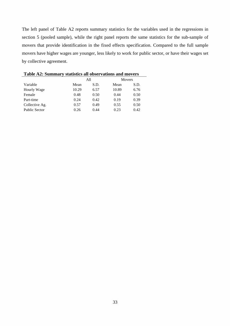
The left panel of Table A2 reports summary statistics for the variables used in the regressions in

section 5 (pooled sample), while the right panel reports the same statistics for the sub-sample of

movers that provide identification in the fixed effects specification. Compared to the full sample

movers have higher wages are younger, less likely to work for public sector, or have their wages set

by collective agreement.

Table A2: Summary statistics all observations and movers All Movers Variable Mean S.D. Mean S.D. Hourly Wage 10.29 6.57 10.89 6.76 Female 0.48 0.50 0.44 0.50 Part-time 0.24 0.42 0.19 0.39 Collective Ag. 0.57 0.49 0.55 0.50 Public Sector 0.26 0.44 0.23 0.42

34

2 Detailed area level results

Table A3 provides a list of the 79 urban areas together with the average wages in 1998 and 2008,

our estimated area effects, predicated average wages based on observed characteristics and

unobserved characteristics. Table A4 provides the same statistics for the 78 rural areas. These are

the data used for figure 1. Table A5 picks out the ten areas with highest and lowest average wages

and area effects.

Table A3: Urban area names, mean area wages, area effects and predicted wages

Area name Wage 1998

Wage 2008

Area average

Area effect

Predicted (observables)

Predicted (unobservables)

Aberdeen 8.77 13.10 0.0311 0.0070 0.0004 0.0227 Barnsley 7.06 9.82 -0.1611 -0.0240 -0.0160 -0.1218 Bedford 8.13 10.95 -0.0128 -0.0051 -0.0002 -0.0086 Birmingham 8.26 11.94 0.0095 0.0126 0.0032 -0.0053 Blackburn 6.88 10.29 -0.1437 -0.0254 -0.0142 -0.1027 Blackpool 7.16 10.58 -0.1288 -0.0480 -0.0140 -0.0674 Bolton 7.71 10.38 -0.1132 -0.0184 -0.0148 -0.0784 Bournemouth 7.61 12.05 -0.0672 -0.0339 -0.0130 -0.0231 Bradford 7.53 10.50 -0.0860 -0.0107 -0.0033 -0.0703 Brighton 8.14 11.95 0.0068 -0.0295 0.0015 0.0362 Bristol 8.55 12.52 0.0343 0.0023 0.0044 0.0273 Burnley, Nelson & Colne 6.70 10.11 -0.1645 -0.0010 -0.0192 -0.1408 Calderdale 7.74 11.92 -0.0052 -0.0006 0.0096 -0.0143 Cambridge 8.80 13.53 0.0905 -0.0014 0.0170 0.0745 Cardiff 7.66 11.28 -0.0436 -0.0082 0.0018 -0.0376 Chelmsford & Braintree 7.89 11.51 -0.0317 -0.0233 -0.0112 0.0011 Cheltenham & Evesham 8.10 11.96 0.0045 -0.0060 -0.0041 0.0148 Colchester 7.64 10.47 -0.0950 -0.0573 -0.0192 -0.0176 Coventry 7.76 11.74 -0.0132 0.0055 -0.0013 -0.0155 Crawley 9.27 12.86 0.0879 0.0303 0.0040 0.0552 Darlington 7.54 10.39 -0.1149 -0.0177 -0.0135 -0.0851 Derby 7.86 12.68 -0.0003 -0.0108 0.0060 0.0034 Doncaster 6.75 10.36 -0.1494 -0.0242 -0.0177 -0.1080 Dudley & Sandwell 7.30 10.27 -0.1259 -0.0089 -0.0172 -0.0988 Dundee 7.80 11.64 -0.0480 -0.0260 0.0051 -0.0266 Edinburgh 8.41 12.92 0.0545 0.0068 0.0153 0.0311 Exeter & Newton Abbot 7.92 11.25 -0.0574 -0.0571 -0.0027 0.0010 Glasgow 7.80 11.74 -0.0435 -0.0061 -0.0025 -0.0357 Gloucester 8.05 11.98 -0.0156 -0.0059 -0.0008 -0.0100 Grimsby 7.31 10.20 -0.1352 -0.0334 -0.0170 -0.0837 Guildford & Aldershot 9.83 14.71 0.1821 0.0480 0.0216 0.1119 Hartlepool 7.02 9.06 -0.1750 -0.0540 -0.0129 -0.1058 Hastings 6.94 9.78 -0.1621 -0.0331 -0.0252 -0.1037 Huddersfield 7.67 11.01 -0.0812 -0.0325 -0.0063 -0.0423 Hull 7.26 10.80 -0.1101 -0.0395 -0.0088 -0.0608 Ipswich 7.72 11.48 -0.0681 -0.0516 -0.0076 -0.0104 Lanarkshire 7.47 11.22 -0.0672 -0.0142 -0.0042 -0.0497 Leeds 7.53 11.75 -0.0393 0.0028 -0.0033 -0.0375 Leicester 7.61 11.12 -0.0677 -0.0216 -0.0077 -0.0379 Liverpool 7.78 11.53 -0.0488 -0.0124 -0.0027 -0.0351 London 10.59 15.93 0.2393 0.0776 0.0241 0.1380 Luton & Watford 8.96 12.86 0.0470 0.0290 -0.0033 0.0196 Maidstone & North Kent 8.06 11.31 -0.0422 0.0008 -0.0143 -0.0286 Manchester 8.19 12.02 0.0124 0.0054 0.0048 0.0012 Mansfield 6.71 10.41 -0.1500 -0.0375 -0.0154 -0.0982

35

Middlesbrough & Stockton 7.18 10.50 -0.1312 -0.0254 -0.0143 -0.0909 Milton Keynes & Aylesbury 9.14 13.16 0.0776 0.0257 0.0068 0.0434 Newcastle & Durham 7.47 10.81 -0.0818 -0.0224 -0.0087 -0.0501 Newport & Cwmbran 7.31 10.44 -0.0921 -0.0143 -0.0112 -0.0657 Northampton & Wellingborough 7.67 11.10 -0.0470 -0.0043 -0.0066 -0.0359 Norwich 7.41 10.94 -0.0766 -0.0311 -0.0088 -0.0370 Nottingham 7.57 11.11 -0.0649 -0.0124 -0.0014 -0.0508 Oxford 8.80 12.91 0.1030 0.0129 0.0191 0.0697 Peterborough 7.69 10.93 -0.0523 -0.0135 -0.0094 -0.0301 Plymouth 6.88 10.77 -0.1082 -0.0687 -0.0105 -0.0299 Poole 8.66 11.29 -0.0297 0.0096 -0.0067 -0.0315 Portsmouth 7.94 12.21 -0.0234 -0.0107 -0.0063 -0.0061 Preston 7.73 11.56 -0.0415 -0.0259 -0.0011 -0.0159 Reading & Bracknell 9.98 15.09 0.2038 0.0527 0.0263 0.1253 Rochdale & Oldham 7.25 10.15 -0.1290 -0.0195 -0.0135 -0.0917 Sheffield & Rotherham 7.53 10.94 -0.0791 -0.0227 -0.0070 -0.0493 Southampton 8.37 12.04 0.0137 0.0004 -0.0035 0.0155 Southend & Brentwood 8.18 11.76 -0.0017 -0.0079 -0.0071 0.0135 Stevenage 9.22 12.72 0.0903 0.0131 0.0122 0.0633 Stoke-on-Trent 7.22 10.16 -0.1479 -0.0407 -0.0125 -0.0934 Sunderland 7.09 10.08 -0.1406 -0.0310 -0.0143 -0.0959 Swansea Bay 7.66 10.35 -0.0985 -0.0401 -0.0085 -0.0499 Swindon 8.47 12.12 0.0257 0.0148 0.0025 0.0090 Telford & Bridgnorth 7.08 11.08 -0.1033 -0.0322 -0.0116 -0.0599 Tunbridge Wells 8.17 12.19 -0.0065 0.0035 -0.0097 0.0010 Wakefield & Castleford 7.68 10.83 -0.0684 0.0011 -0.0085 -0.0599 Walsall & Cannock 7.26 10.44 -0.1288 -0.0278 -0.0129 -0.0862 Warrington & Wigan 7.71 11.41 -0.0655 -0.0300 -0.0050 -0.0300 Wirral & Ellesmere Port 8.00 10.54 -0.0764 -0.0267 -0.0124 -0.0361 Wolverhampton 7.40 10.15 -0.0999 -0.0215 -0.0082 -0.0686 Worcester & Malvern 7.36 10.75 -0.0871 -0.0440 -0.0041 -0.0400 Worthing 8.23 11.45 -0.0296 -0.0367 -0.0038 0.0113 Wycombe & Slough 9.74 14.15 0.1709 0.0527 0.0187 0.1002 York 7.51 11.74 -0.0668 -0.0259 -0.0104 -0.0304 Notes: Area effects, average area predicted wage based on observables and unobservable from regression of log wages on fixed effects and observables (set of age dummies and a set of 1 digit occupation dummies)

36

Table A4: Rural area names, mean area wages, area effects and predicted wages

Area name Wage 1998

Wage 2008

Area average

Area effect

Predicted (observables)

Predicted (unobservables)

Andover 8.42 12.24 0.0129 -0.0133 -0.0007 0.0277 Ayr & Kilmarnock 7.49 10.53 -0.1010 -0.0403 -0.0092 -0.0506 Banbury 8.44 11.52 -0.0153 0.0107 -0.0098 -0.0152 Basingstoke 9.39 13.89 0.1484 0.0222 0.0136 0.1130 Bath 8.16 11.77 -0.0090 -0.0185 0.0047 0.0048 Brecon and South Mid Wales 7.31 9.94 -0.1592 -0.0680 -0.0181 -0.0729 Bridgend 7.07 11.04 -0.1073 -0.0187 -0.0101 -0.0792 Burton upon Trent 7.02 10.79 -0.1207 -0.0266 -0.0123 -0.0837 Canterbury 7.11 10.67 -0.0926 -0.0569 -0.0101 -0.0271 Carlisle 6.96 10.40 -0.1440 -0.0137 -0.0142 -0.1160 Chester & Flint 8.16 10.54 -0.0444 -0.0305 -0.0044 -0.0102 Chesterfield 7.25 10.34 -0.1345 -0.0351 -0.0130 -0.0836 Chichester & Bognor Regis 7.77 11.21 -0.0748 -0.0626 -0.0099 -0.0061 Crewe & Northwich 7.81 11.23 -0.0640 -0.0293 -0.0109 -0.0266 Dorset-Devon Coast 6.88 10.99 -0.1238 -0.0615 -0.0135 -0.0521 Dunfermline 7.66 11.01 -0.0941 -0.0188 -0.0060 -0.0691 East Anglia Coast - Gt Yarmouth and Lowestoft 6.69 10.38 -0.1550 -0.0569 -0.0172 -0.0806 East Anglia West - Bury and Thetford 6.94 10.60 -0.1320 -0.0492 -0.0237 -0.0602 East Cornwall 6.99 9.12 -0.2074 -0.0832 -0.0254 -0.1005 East Highlands 6.97 10.20 -0.1740 -0.0404 -0.0193 -0.1139 East Kent - Dover and Margate 7.54 10.10 -0.0947 -0.0360 -0.0153 -0.0423 East Lincolnshire 7.10 10.51 -0.1408 -0.0456 -0.0200 -0.0749 East North Yorkshire 6.46 10.43 -0.1749 -0.0631 -0.0244 -0.0884 East Somerset - Bridgwater and Wells 7.36 10.51 -0.1218 -0.0495 -0.0223 -0.0500 Eastbourne 7.29 11.25 -0.0840 -0.0523 -0.0187 -0.0134 Falkirk 7.30 10.56 -0.1011 -0.0197 -0.0095 -0.0719 Greenock, Arran and and Irvine 7.69 10.75 -0.1142 -0.0282 -0.0079 -0.0769 Harlow & Bishop's Stortford 8.84 13.28 0.0791 0.0226 0.0027 0.0530 Harrogate 7.73 11.48 -0.0611 -0.0330 -0.0031 -0.0266 Hereford & Leominster 6.95 10.14 -0.1435 -0.0541 -0.0153 -0.0744 Huntingdon 8.07 11.85 0.0039 -0.0144 0.0038 0.0149 Inverness 7.60 10.83 -0.0751 -0.0437 0.0019 -0.0375 Isle of Wight 7.18 9.99 -0.1355 -0.0687 -0.0228 -0.0428 Kendal 7.01 10.60 -0.1230 -0.0668 -0.0012 -0.0545 Kettering & Corby 7.20 9.97 -0.1262 -0.0232 -0.0244 -0.0782 Lancaster & Morecambe 7.88 11.53 -0.0581 -0.0555 -0.0053 0.0031 Livingston & Bathgate 7.04 10.78 -0.0944 -0.0033 -0.0113 -0.0834 Mid North East England 7.29 10.24 -0.1413 -0.0470 -0.0141 -0.0764 Mid Wales 6.97 10.02 -0.1627 -0.0727 -0.0215 -0.0680 Mid Wales Border 6.88 9.86 -0.1824 -0.0544 -0.0225 -0.1042 Moray Firth 7.03 10.14 -0.1696 -0.0412 -0.0176 -0.1113 Morpeth, Ashington & Alnwick 7.06 10.69 -0.1310 -0.0354 -0.0101 -0.0841 Newbury 9.36 13.84 0.1463 0.0237 0.0171 0.1079 Norfolk, Linolnshire Fens 6.57 9.38 -0.1991 -0.0469 -0.0250 -0.1278 North Cumbria 6.30 9.53 -0.2177 -0.0802 -0.0281 -0.1097 North Devon 6.67 10.63 -0.1707 -0.0632 -0.0253 -0.0829 North Firth of Forth 7.48 10.84 -0.1025 -0.0069 -0.0148 -0.0819 North Norfolk 7.12 9.76 -0.1585 -0.0491 -0.0268 -0.0815 North Scotland 7.70 11.71 -0.0676 0.0049 -0.0092 -0.0633 North Solway Firth 6.72 10.69 -0.1326 -0.0170 -0.0158 -0.1023

37

North Wales Coast 6.89 10.39 -0.1494 -0.0538 -0.0164 -0.0806 North West Devon 6.45 9.55 -0.2410 -0.0805 -0.0371 -0.1244 North West Wales 7.12 10.20 -0.1164 -0.0141 -0.0150 -0.0898 Perth & Blairgowrie 7.20 10.71 -0.1124 -0.0035 -0.0116 -0.1005 Rugby 7.87 11.67 -0.0042 -0.0023 -0.0099 0.0059 Salisbury, Shaftesbury and Blandford 7.23 11.44 -0.0938 -0.0243 -0.0088 -0.0632 Scarborough, Bridlington and Driffield 6.81 9.22 -0.1899 -0.0598 -0.0267 -0.1030 Scottish Borders 7.04 10.19 -0.1721 -0.0261 -0.0154 -0.1304 Scunthorpe 7.49 10.38 -0.1207 -0.0377 -0.0059 -0.0748 Shrewsbury 7.09 10.83 -0.1049 -0.0403 -0.0141 -0.0517 South Cumbria 7.88 12.00 0.0094 -0.0194 0.0069 0.0231 South Devon 6.38 9.90 -0.2093 -0.0757 -0.0331 -0.1021 South Wales Border 6.84 10.30 -0.1433 -0.0307 -0.0129 -0.0959 South West Wales 7.17 10.63 -0.1535 -0.0797 -0.0133 -0.0626 Stafford 7.42 11.62 -0.0323 -0.0410 0.0048 0.0035 Stirling & Alloa 7.45 11.06 -0.0767 0.0077 -0.0041 -0.0805 Taunton 7.62 11.02 -0.0800 -0.0644 -0.0101 -0.0082 Trowbridge & Warminster 7.21 11.48 -0.1004 -0.0204 -0.0178 -0.0611 Warwick & Stratford-upon-Avon 8.62 13.05 0.0425 -0.0152 0.0107 0.0456 West Cornwall 6.33 10.27 -0.1869 -0.0771 -0.0154 -0.0950 West Kent - Ashford and Folkestone 7.78 10.87 -0.0841 -0.0230 -0.0200 -0.0403 West Lincolnshire 6.94 9.72 -0.1945 -0.0504 -0.0260 -0.1163 West North Yorkshire 6.91 10.17 -0.1546 -0.0191 -0.0206 -0.1138 West Peak District - Matlock and Buxton 6.89 10.82 -0.0955 -0.0496 -0.0077 -0.0384 Western Highlands 6.86 10.74 -0.1114 -0.0371 -0.0152 -0.0588 Worksop & Retford 7.23 10.00 -0.1359 -0.0197 -0.0176 -0.0956 Wrexham & Whitchurch 7.30 10.36 -0.1193 -0.0464 -0.0149 -0.0573 Yeovil & Chard 7.53 10.89 -0.0693 -0.0517 -0.0037 -0.0131 Notes: Area effects, average area predicted wage based on observables and unobservable from regression of log wages on fixed effects and observables (set of age dummies and a set of 1 digit occupation dummies)

38

Table A5. Areas with highest and lowest wages and area effects Top 10 area averages (with 2008 wages) Top 10 area effects London 22.6% London 7.8% Reading & Bracknell 19.1% Wycombe & Slough 5.3% Guildford & Aldershot 17.0% Reading & Bracknell 5.3% Wycombe & Slough 16.1% Guildford & Aldershot 4.8% Basingstoke 13.9% Crawley 3.0% Newbury 14.0% Luton & Watford 2.9% Oxford 9.9% Milton Keynes & Aylesbury 2.6% Cambridge 8.7% Newbury 2.4% Stevenage 9.1% Harlow & Bishop's Stortford 2.3% Crawley 9.0% Basingstoke 2.2% Bottom 10, 1998 Hartlepool -17.5% Brecon and South Mid Wales -6.8% Mid Wales Border -18.2% Isle of Wight -6.9% West Cornwall -18.7% Plymouth -6.9% Scarborough, Bridlington and Driffield -19.0% Mid Wales -7.3% West Lincolnshire -19.5% South Devon -7.6% Norfolk, Linolnshire Fens -19.9% West Cornwall -7.7% East Cornwall -20.7% South West Wales -8.0% South Devon -20.9% North Cumbria -8.0% North Cumbria -21.8% North West Devon -8.1% North West Devon -24.1% East Cornwall -8.3% Notes: Area averages for 1998-2008 and area effects from regression of log wages on area effects, individual effects and observables (set of age dummies and a set of 1 digit occupation dummies) reported as percentage above or below reference area (Southampton, ranked 19th for area averages and 28th)

39

3 Geographical units

The figures show the 157 geographical units (aggregations of TTWAs) that we use in our analysis

Rural TTWA aggregates Primary urban TTWAs

40

4 Rural versus urban

Table A.6 shows results from regressions of wage on individual characteristics for the urban and

rural areas separately, and for all areas pooled. Results are for a specification that includes a dummy

for gender, a set of dummies for age, and for one digit occupation. The coefficients and standard

errors suggest there are differences between the samples.

Table A.6: Wage regressions for urban, rural and all areas. Variables Urban Rural All Female -0.1458 (0.0007)*** -0.1581 (0.0013)*** -0.1480 (0.0006)*** Age group 2 0.1465 (0.0018)*** 0.1243 (0.0034)*** 0.1419 (0.0016)*** Age group 3 0.2754 (0.0017)*** 0.2317 (0.0033)*** 0.2669 (0.0015)*** Age group 4 0.3487 (0.0017)*** 0.2959 (0.0032)*** 0.3385 (0.0015)*** Age group 5 0.3749 (0.0017)*** 0.3239 (0.0032)*** 0.3648 (0.0015)*** Age group 6 0.3800 (0.0017)*** 0.3357 (0.0032)*** 0.3712 (0.0015)*** Age group 7 0.3807 (0.0017)*** 0.3387 (0.0032)*** 0.3722 (0.0015)*** Age group 8 0.3615 (0.0017)*** 0.3238 (0.0032)*** 0.3539 (0.0015)*** Age group 9 0.3192 (0.0018)*** 0.2848 (0.0034)*** 0.3125 (0.0016)*** Age group 10 0.2530 (0.0023)*** 0.2201 (0.0040)*** 0.2466 (0.0020)*** Occupations (rev. 1990) Professional 0.1501 (0.0020)*** 0.2309 (0.0041)*** 0.1639 (0.0018)*** Technical -0.1428 (0.0021)*** -0.1186 (0.0043)*** -0.1393 (0.0019)*** Administrative -0.5256 (0.0018)*** -0.4871 (0.0036)*** -0.5198 (0.0016)*** Skilled trades -0.5350 (0.0022)*** -0.5082 (0.0041)*** -0.5318 (0.0019)*** Personal Services -0.6540 (0.0021)*** -0.5924 (0.0040)*** -0.6436 (0.0019)*** Sales -0.7160 (0.0022)*** -0.6615 (0.0044)*** -0.7074 (0.0020)*** Manufacturing -0.6744 (0.0021)*** -0.6119 (0.0039)*** -0.6630 (0.0019)*** Elementary -0.8423 (0.0023)*** -0.7578 (0.0042)*** -0.8261 (0.0020)*** Occupations (rev. 2003) Professional 0.1074 (0.0015)*** 0.2145 (0.0031)*** 0.1257 (0.0014)*** Technical -0.2187 (0.0015)*** -0.1472 (0.0030)*** -0.2068 (0.0013)*** Administrative -0.5050 (0.0014)*** -0.4411 (0.0029)*** -0.4947 (0.0013)*** Skilled trades -0.5586 (0.0018)*** -0.4946 (0.0033)*** -0.5483 (0.0016)*** Personal Services -0.6924 (0.0019)*** -0.5941 (0.0033)*** -0.6745 (0.0016)*** Sales -0.7928 (0.0017)*** -0.7091 (0.0033)*** -0.7788 (0.0015)*** Manufacturing -0.7031 (0.0018)*** -0.6123 (0.0032)*** -0.6864 (0.0016)*** Elementary -0.8358 (0.0015)*** -0.7155 (0.0029)*** -0.8129 (0.0014)*** Constant 2.1569 (0.0022)*** 2.0702 (0.0043)*** 2.1412 (0.0019)*** Observations 1208698 302174 1510872 R-squared 0.595 0.587 0.596 Notes: Results for urban, rural and pooled sample based on classification described in the text.

Looking at the results, we see that women are paid less than men in all areas, but that the effect is

slightly more pronounced in urban areas. The coefficients on the age group dummies report the

effect of age on wages relative to the omitted category (age 16-20). They show that in both urban

and rural areas, wages rise with age until workers reach their 40s and then decline but that the effect

of age is slightly more pronounced in urban than in rural areas. The coefficients on occupations also

41

give the effect relative to the omitted category (managers and senior officials). As explained in the

text, the classification in the data changes over time, although they are fairly comparable at the one

digit level we use here. The pattern of coefficients show that in both rural and urban areas

professional occupations pay a premium relative to managerial occupations (the positive coefficient

on the professional dummy) but that managerial occupations pay a premium relative to the

remaining categories (the negative coefficients on the other occupations). The professional

occupation premium is more pronounced in rural areas (the coefficient on the professional dummy

is larger) but managerial premium is lower (the negative coefficients on the other occupations are

smaller). Explaining these differences is beyond the scope of this paper, but we do take them in to

account by allowing the effect of individual observables to differ between the two different samples

in the results reported in the text.

As described in the text, our classification of areas in to rural and urban was based on the urban

footprint of primary urban areas and sample sizes in our data set (with any area with a large enough

sample being classified as non-primary urban). With the data available, sample size restrictions

prevent us from using smaller areas (we are already forced to aggregate up smaller TTWA as

described in the text). We are, however, able to consider differences between rural and urban

postcodes locations within our 157 labour market areas. To do this, we can run the same regression

as above, but include a rural dummy. That is:

iruraliii dxw '')ln(

where theta is a dummy variable that takes value 1 when the worker works in a rural postcode

(defined according to whether the postcode is part of a settlement with more or less than 10,000

people). This classification is based on the ONS rural/urban definition introduced in 2004. The

definition is based on a settlement based approach and comprises four settlement types (urban; town

and fringe; village; hamlet and isolated dwelling). To ensure sufficient sample sizes we aggregate

the three rural settlement types and define rural locations as any location not classified as urban.

If we do not include area effects or any individual characteristics, the coefficient on theta (the rural

dummy) tells us how much lower wages are for workers in rural postcodes. When we control for

individual characteristics, we can see whether this effect is due to the sorting of workers between

rural and urban postcodes. Including area dummies for our 157 areas tells us about the effect of

working in a rural postcode compared to “nearby” urban postcodes (e.g. the effect of working in a

rural location in North Cornwall, relative to working in an urban location in North Cornwall). Table

42

A.7 reports results for various specifications. The first column reports the raw effects without

controlling for individual characteristics, the second and third column add individual characteristics

(as in the text), while the fourth to sixth columns add individual fixed effects (again, as in the text).

The final three columns drop individual fixed effects, but include area effects (for the 157

aggregations of TTWA).

Reading across the table we see that the raw urban-rural premium is 8.4%. This is slightly higher

than the 6.5% urban-rural area premium reported in the first row of Table 6 in the main text. In

terms of simple averages, urban-rural location matters slightly more for wages than the urban-rural

area classification used in the text. Controlling for basic observable characteristics of individuals

nearly halves the estimate to 4.5%, broadly in line with the 4.2% urban-rural area premium reported

in the second column of Table 6 in the main text. This again demonstrates the importance of sorting

on observable characteristics. Allowing for unobserved individual characteristics reduces the

premium further with our lowest estimate on the basis of controlling for observed and unobserved

individual characteristics suggesting an urban-rural postcode premium of 1.5%, now slightly lower

than the 2.4% for the urban-rural area difference reported in the fifth row of Table 6. The fact that

the premium for an urban postcode falls further than that for the urban area premium (from 8.4% to

1.5% compared to 6.5% to 2.4%) suggests that sorting plays slightly more of a role in explaining

the lower wages paid in urban postcodes. The final three columns show that this effect is reduced

further once we allow for the fact that urban areas pay a 2.4% premium over rural areas. Controlling

for observed individual characteristics and area effects (but not individual unobserved

characteristics) we estimate an urban location premium of 0.6 of a percentage point. That is, jobs in

rural postcodes pay only 0.6% less than nearby urban postcodes within the same labour market

area. We would expect these effects to be even smaller if we controlled for unobserved individual

characteristics (which we cannot do due to computational limitations). We conclude that focusing

on 157 labour market areas does not disguise large disparities between urban and rural locations

within these labour market areas .

Table A.7: Coefficient on rural dummy (various specifications) (1) (2) (3) (4) (5) (6) (7) (8) (9)

rural10k -0.0842*** -0.0620*** -0.0454*** -0.0198*** -0.0189*** -0.0154*** -0.0191*** -0.0190*** -0.0062***

0.0012 0.0008 0.0007 0.0009 0.0009 0.0008 0.0012 0.0008 0.0008 Notes: Reports coefficient and standard error on rural dummy for 9 specifications. Specification (1) includes only year dummies; (2) adds age, gender, 1 digit occupation to (1); (3) adds age, gender, 2 digit occupation, 3 digit sic, and dummies for public sector, collective agreement and part time workers to (1); (4) includes only year dummies and individual fixed effects; (5) adds age and 1 digit occupation to (4); (6) adds dummies for public sector, collective agreement and part time workers to (5); (7) includes year dummies, individual fixed affects and area dummies; (8) adds age, gender, 1 digit occupation to (7); (9) adds dummies for public sector, collective agreement and part time workers to (8)

43

5 Notes on variance decomposition in the context of area effects

5.1 Introduction

Consider the linear regression model for log wages ln iw

ln i i i iw x d (1)

where ix are individual characteristics and id is an "area effect" in which id is a J x 1 column

vector of J area dummies, and is a J x 1 vector of parameters. Our aim is to find the contribution of id to the total variance of ln iw .

Note that

ˆ ˆ ˆln

ˆ ˆ ˆ ˆ ˆ2 ,

i i i i

i i i i i

Var w Var x d

Var x Var d Cov x d Var

(2)

where .Var is taken to mean the sample variance and is the residual. Alternatively,

ˆ ˆ ˆ ˆ2 , ˆ1

ln ln ln ln

i i i i i

i i i i

Var x Var d Cov x d Var

Var w Var w Var w Var w

(3)

and

2

ˆ ˆ ˆ ˆ2 ,ln ; ,

ln ln ln

i i i i

i i ii i i

Var x Var d Cov x dR w x d

Var w Var w Var w

(4)

Here the notation 2 ˆ ˆln ; ,i i iR w x d means the R-squared from a regression of iy on ix and id

Consider now some ways to decompose ln iVar w into components attributable to ix and id

5.2 Method A. Uncorrelated Variance Share

The following methods give the same result which we refer to in the main text as the uncorrelated

variance share. This is sometimes referred to as the semi-partial R-squared and by Borcard (2002)

as "Fraction a" partitioning:

44

a) R-squared method:

(i) Regress iy on ix and id to get 2 ˆ ˆln ; ,i i iR w x d

(ii) Regress iy on ix and get 2 ˆln ;i iR w x

(iii) Calculate 2 ˆ ˆln ; ,i i iR w x d – 2 ˆln ;i iR w x

b) Note that

2 2

ˆ ˆ ˆln ; , ln ;ˆ ˆ ˆln ; , ln ;

ln

i i i i i

i i i i ii

RSS w x d RSS w xR w x d R w x

TSS w

in

which RSS is Regression Sum of Squares and TSS is the total sum of squares. The numerator in this

expression is the Partial Sum of Squares of d . All these sums of squares are routinely computed by

standard ANOVA software

c) Partitioned regression:

(i) Regress ln iw on ix and id and predict ˆid and ˆ

ix

(ii) Regress predicted ˆid on ˆ

ix and obtain the residual ˆ ˆ ˆˆi i iu d x

(iii) Regress iy on the residual ˆiu from (ii) and look at the R-squared 2 ˆln ;i iR w u or

simply square the Pearson correlation coefficient of ln iw and ˆiu

Proof that a) and c) are equivalent (b, follows by definition of the Partial Sum of Squares):

Let sample regression of ˆid on ˆ

ix be

ˆ ˆ ˆ ˆi i id x u (5)

Which implies, from (1)

ˆ ˆ ˆ ˆˆln i i i i iw x x u (6)

From (4) and (5)

2ˆ ˆ ˆ ˆ2 ,

ˆ ˆln ; ,ln ln ln

ˆ ˆ ˆ ˆ2

ln ln ln

i i i i

i i ii i i

i i i

i i i

Var x Var d Cov x dR w x d

Var w Var w Var w

Var x Var d Var x

Var w Var w Var w

(7)

45

Now, from equation (6),

2

2

ˆ ˆ1ˆln ;

ln

ˆ ˆ ˆ1 2

ln

i

i ii

i

i

Var xR w x

Var w

Var x

Var w

(8)

So from (7) and (8) we have:

2

2 2ˆ ˆ ˆ

ˆ ˆ ˆln ; , ln ;ln

i i

i i i i ii

Var d Var xR w x d R w x

Var w

(9)

Now in Method A c) (iii)

2ˆ

ˆln ;ln

ii i

i

Var uR w u

Var w (10)

Where the numerator is

2

2

2

ˆ ˆ ˆ ˆ ˆ ˆˆ 2 ,

ˆ ˆ ˆ ˆ ˆ2

ˆ ˆ ˆ

i i i i i

i i i

i i

Var u Var d Var x Cov x d

Var d Var x Var x

Var d Var x

(11)

Hence from (9)-(11) the uncorrelated variance share is:

2

2 2 2ˆ ˆ ˆ

ˆ ˆ ˆˆln ; ln ; , ln ;ln

i i

i i i i i ii

Var d Var xR w u R w x d R w x

Var w

(12)

And so the Method A c) and A a) are equivalent.

All of these methods consider only the component of the area effect id that is orthogonal to

(uncorrelated with) individual characteristics ix (e.g. if London is has a high wage effect and high

skills, then the correlation of the area effect with individual skills is partialled out).

Note, for comparison, another similar measure is the ‘partial R-squared’. This measures the share of

the components of area effects that are uncorrelated with ix , in the components of ln iw that are

uncorrelated with ix . The partial R-squared is:

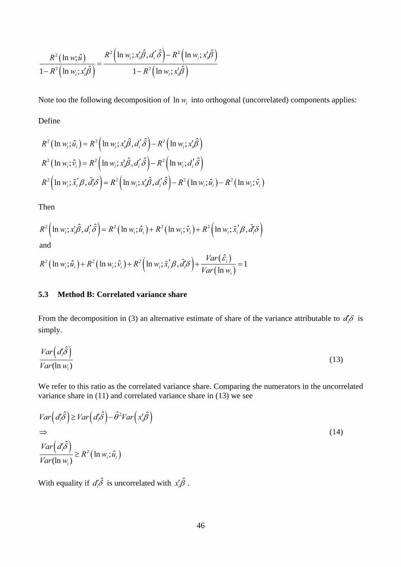
46

2 22

2 2

ˆ ˆ ˆln ; , ln ;ˆln ;

ˆ ˆ1 ln ; 1 ln ;

i i i i i

i i i i

R w x d R w xR w u

R w x R w x

Note too the following decomposition of ln iw into orthogonal (uncorrelated) components applies:

Define

2 2 2

2 2 2

2 2 2 2

ˆ ˆ ˆˆln ; ln ; , ln ;

ˆ ˆ ˆˆln ; ln ; , ln ;

ˆ ˆ ˆ ˆln ; , ln ; , ln ; ln ;

i i i i i i i

i i i i i i i

i i i i i i i i i i

R w u R w x d R w x

R w v R w x d R w d

R w x d R w x d R w u R w v

Then

2 2 2 2

2 2 2

ˆ ˆ ˆ ˆln ; , ln ; ln ; ln ; ,

and

ˆˆ ˆln ; ln ; ln ; , 1

ln

i i i i i i i i i i

ii i i i i i i

i

R w x d R w u R w v R w x d

VarR w u R w v R w x d

Var w

5.3 Method B: Correlated variance share

From the decomposition in (3) an alternative estimate of share of the variance attributable to id is

simply.

ˆ(ln )

i

i

Var d

Var w

(13)

We refer to this ratio as the correlated variance share. Comparing the numerators in the uncorrelated variance share in (11) and correlated variance share in (13) we see

2

2

ˆ ˆ ˆ ˆ

ˆˆln ;

(ln )

i i i

i

i ii

Var d Var d Var x

Var dR w u

Var w

(14)

With equality if ˆid is uncorrelated with ˆ

ix .

47

Therefore the correlated variance share from Method B yields an answer for the contribution of id

that is bigger than that obtained by the uncorrelated variance share in Method A.

5.4 Method C: Standard deviations × correlation

Another method has been used in some previous studies e.g. Borcard (2002) Method 1 and Combes,

Duranton Gobillon (2008).

Note that, if . . .s d .r are the sample standard deviation and Pearson correlation coefficient

2

ˆ ˆ. . . .ˆ ˆln , ln ,

. . ln . . ln

ˆ ˆln , ln ,

ln ln

ˆ ˆ ˆ ˆ2 ,

ln ln ln

ˆ ˆln ; ,

i i

i i i ii i

i i i i

i i

i i i i

i i i

i i i

s d x s d dr w x r w d

s d w s d w

Cov w x Cov w d

Var w Var w

Var x Var d Cov x d

Var w Var w Var w

R w x d

(13)

Hence

ˆ ˆ ˆ ˆ ˆ. . ln , ,ˆln ,

. . ln ln ln

i i i i i i

i ii i i

s d d Cov w x Var d Cov x dr w d

s d w Var w Var w

(14)

Provides yet another possible measure of the share attributable to id

Inspection of the share in Method C (14) and Method B (11) shows that Method C simply adds

,i iCov x d to the correlated variance share. Hence, with positive covariance between ix and

id , Method C must give you a bigger number than the correlated variance share for the partial

contribution of id . All methods give the same result if ix and id are uncorrelated.

Extension to individual and area fixed effects

All the methods can be extended to allow for multiple groups of effects f .

ln i fi if

w

48

Then the uncorrelated variance shares (semi-partial 2R ) are 2 2~ ~ˆ ˆ ˆln ; , ln ;i fi fi i fiR w R w and

2 2 2 2~ ~ ~ ~

ˆˆ ˆ ˆ ˆ ˆ ˆln ; , ln ; ln ; , ln ; 1

lni

i fi fi i fi i fi fi i fif f i

VarR w R w R w R w

Var w

Here, the notation ~ˆ

fi means all effects not including fi .

For the correlated variance shares

ˆ

lnfi

i

Var

Var w

:

ˆ ˆ ˆ, ˆ1

ln ln lnfi fi gi i

f f gi i i

Var Cov Var

Var w Var w Var w

The stata routine a2reg for two way fixed effects (Ouazad 2008) is useful for practical

implementation and is based on Abowd, Creecy and Kramarz (2002)

http://courses.cit.cornell.edu/jma7/abowd-creecy-kramarz-computation.pdf)

Spatial Economics Research Centre (SERC)London School of EconomicsHoughton StreetLondon WC2A 2AE

Tel: 020 7852 3565Fax: 020 7955 6848Web: www.spatialeconomics.ac.uk

SERC is an independent research centre funded by theEconomic and Social Research Council (ESRC), Departmentfor Business, Enterprise and Regulatory Reform (BERR),the Department for Communities and Local Government(CLG) and the Welsh Assembly Government.