IZA DP No. 1776

Wage Ceilings and Floors:The Gender Gap in Ukraine's Transition

Ina GanguliKatherine Terrell

DI

SC

US

SI

ON

PA

PE

R S

ER

IE

S

Forschungsinstitutzur Zukunft der ArbeitInstitute for the Studyof Labor

September 2005

Wage Ceilings and Floors:

The Gender Gap in Ukraine’s Transition

Ina Ganguli Harvard University

Katherine Terrell

University of Michigan, Ann Arbor and IZA Bonn

Discussion Paper No. 1776 September 2005

IZA

P.O. Box 7240 53072 Bonn

Germany

Phone: +49-228-3894-0 Fax: +49-228-3894-180

Email: iza@iza.org

Any opinions expressed here are those of the author(s) and not those of the institute. Research disseminated by IZA may include views on policy, but the institute itself takes no institutional policy positions. The Institute for the Study of Labor (IZA) in Bonn is a local and virtual international research center and a place of communication between science, politics and business. IZA is an independent nonprofit company supported by Deutsche Post World Net. The center is associated with the University of Bonn and offers a stimulating research environment through its research networks, research support, and visitors and doctoral programs. IZA engages in (i) original and internationally competitive research in all fields of labor economics, (ii) development of policy concepts, and (iii) dissemination of research results and concepts to the interested public. IZA Discussion Papers often represent preliminary work and are circulated to encourage discussion. Citation of such a paper should account for its provisional character. A revised version may be available directly from the author.

IZA Discussion Paper No. 1776 September 2005

ABSTRACT

Wage Ceilings and Floors: The Gender Gap in Ukraine’s Transition∗

This paper uses new micro data from the Ukrainian Longitudinal Monitoring Survey (ULMS) to examine the gender gaps across the distribution of wages in Ukraine during communism (1986), the start of transition (1991), and after Ukraine started to be considered a market economy (2003). We find that the gender pay gap is higher in the top half of the distribution than at the bottom half and that this ‘glass ceiling’ is persistent across the three points in time, while the wage floor rose for women in 2003. Closer inspection of two sectors – the private and the public – reveals the striking finding that the glass ceiling is lower in the public than in the private sector but the floor is the same. We use the Machado and Mata (2004) method to create counterfactuals that advance our knowledge of which factors are driving these differences; we find that the differences in men’s and women’s rewards (βs) rather than differences in their productive characteristics (Xs) explain most of the wage gap throughout the distribution. The different ceilings in the public and private sectors are largely due to differences in men’s and women’s productive characteristics, which favor men in the public and women in the private sector. The fall in the gender gap in the lower part of the distribution from 1986 to 2003 is explained partially by the improvement in women’s productive characteristics and partially by the worsening in men’s rewards in the bottom half of the distribution over time. However, probably the most important reason for the reduction in the gap at the bottom of the distribution over time is that the value of the minimum wage was set relatively high in 2003 and it raised the wage floor for more women than men. JEL Classification: C14, I2, J16 Keywords: gender gap, quantile regression, glass ceilings, glass floors, transition, Ukraine Corresponding author: Katherine Terrell University of Michigan Business School 701 Tappan Street, 7th Floor Ann Arbor, MI 48109 USA Email: terrell@umich.edu

∗ The authors would like to thank Kathryn Anderson, Olivier Deschenes, John DiNardo, Yuriy Gorodnichenko, Jennifer Hunt, David Margolis, Andrew Newell, and Jan Svejnar for their comments as well as participants of the ACES session at the ASSA meetings in Philadelphia, Jan. 6-9, 2005, the EBRD/IZA Conference in Bologna, May 5-6, 2005 and the SOLE-EALE meetings in San Francisco, June 2-5, 2005. Katherine Terrell is grateful to the NSF (Research Grant SES 0111783) for its generous support. Ina Ganguli appreciates the support of the U.S. Fulbright Program and the EERCEROC at the National University “Kyiv-Mohyla Academy.” We also thank Joseph Green, Olga Kupets, and Bogdan Prokopovych for their assistance.

- 2 -

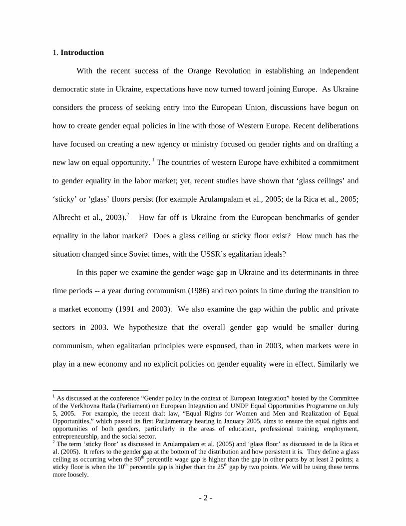
1. Introduction

With the recent success of the Orange Revolution in establishing an independent

democratic state in Ukraine, expectations have now turned toward joining Europe. As Ukraine

considers the process of seeking entry into the European Union, discussions have begun on

how to create gender equal policies in line with those of Western Europe. Recent deliberations

have focused on creating a new agency or ministry focused on gender rights and on drafting a

new law on equal opportunity. 1 The countries of western Europe have exhibited a commitment

to gender equality in the labor market; yet, recent studies have shown that ‘glass ceilings’ and

‘sticky’ or ‘glass’ floors persist (for example Arulampalam et al., 2005; de la Rica et al., 2005;

Albrecht et al., 2003).2 How far off is Ukraine from the European benchmarks of gender

equality in the labor market? Does a glass ceiling or sticky floor exist? How much has the

situation changed since Soviet times, with the USSR’s egalitarian ideals?

In this paper we examine the gender wage gap in Ukraine and its determinants in three

time periods -- a year during communism (1986) and two points in time during the transition to

a market economy (1991 and 2003). We also examine the gap within the public and private

sectors in 2003. We hypothesize that the overall gender gap would be smaller during

communism, when egalitarian principles were espoused, than in 2003, when markets were in

play in a new economy and no explicit policies on gender equality were in effect. Similarly we

1 As discussed at the conference “Gender policy in the context of European Integration” hosted by the Committee of the Verkhovna Rada (Parliament) on European Integration and UNDP Equal Opportunities Programme on July 5, 2005. For example, the recent draft law, “Equal Rights for Women and Men and Realization of Equal Opportunities,” which passed its first Parliamentary hearing in January 2005, aims to ensure the equal rights and opportunities of both genders, particularly in the areas of education, professional training, employment, entrepreneurship, and the social sector. 2 The term ‘sticky floor’ as discussed in Arulampalam et al. (2005) and ‘glass floor’ as discussed in de la Rica et al. (2005). It refers to the gender gap at the bottom of the distribution and how persistent it is. They define a glass ceiling as occurring when the 90th percentile wage gap is higher than the gap in other parts by at least 2 points; a sticky floor is when the 10th percentile gap is higher than the 25th gap by two points. We will be using these terms more loosely.

- 3 -

might expect the gap to be smaller in the public sector than in the private sector, if the

government applies more egalitarian principles to its wage setting than the competitive market

forces which drive wages in the private sector. If that is the case, then we would anticipate the

overall gender gap to widen as employment in the private sector grows. However, it is also

possible that, at least in some economic activities, competitive forces are strong enough to stifle

discriminatory practices as found by Black and Brainerd (1999) and Weischselbaumer and

Winter-Ebmer (2003). Finally, we also examine the public and private sectors separately since

the government may want to see that its own house is in order before asking for compliance

with new wage polices from the private sector.

Hence, we seek to advance our understanding of the size and determinants of the wage

gaps and assist policymakers in the process of formulating more gender equal policies. We

analyze the gender gap at the mean and across the wage distribution to see if there are ‘glass

ceilings’ and ‘sticky floors’ for women in Ukraine. We examine the extent to which these

differentials are based on discrimination, measured as different returns for men and women for

a unit of the same productive characteristic. We also ask to what extent the gaps are due to

differences in the composition of men and women’s labor force (in terms of human capital and

job characteristics) in a given year or sector since we expect that the transition to markets

changed substantially the composition of people and jobs in the labor market. Finally, we ask to

what extent institutions, such as the minimum wage, have played a role in the gender gap.

We apply the Machado and Mata (2004) decomposition method to new household data

from the 2003 Ukrainian Longitudinal Monitoring Survey (ULMS) and find that the male-

female wage gap is larger at the top than at the bottom of the distribution and that the gap

remained fairly constant in all parts of the distribution in 1986 and 1991, but that it fell

- 4 -

substantially in the lower part of the distribution in 2003. It seems that the reason that the floor

is less sticky in 2003 compared to 1986 and 1991 is due to government intervention. In 2003,

the minimum wage is set at a level that is binding for women’s wages but not binding for most

men in the bottom half of the distribution. Moreover, the counterfactual analysis indicates that

the improvement in the wage gap at the bottom of the distribution is driven by the better

composition of women’s characteristics relative to men’s in 2003, compared to 1986 and 1991.

A striking finding is that the gaps in private sector are smaller than the gaps public

sector in the top half of the distribution. Our decomposition results indicate that the low glass

ceiling in the public sector is also being driven by women’s unfavorable characteristics

compared to men in that sector; women in the private sector have more favorable

characteristics compared to men, which compensated them for the lower returns for the same

characteristic. Nevertheless, there is substantial evidence in each year and in each sector that

the most important force driving the gender gaps throughout the distribution are differential

rewards, or discrimination.

The paper is structured as follows: A brief review of the literature is presented in

Section 2; Ukraine’s transition experience is described in Section 3; an explanation of the data

source is found in Sections 4; the observed wage gaps are described in Section 5, and analyzed

with counterfactuals in Section 6; the impact of the minimum wage is discussed in Section 7;

conclusions follow in Section 8.

2. Literature Review

There is a large body of research dealing with the extent to which the gap between

men’s and women’s wages has grown in the transition countries as the market-based economies

replaced the planned economies (see for example, Anderson and Pomfret, 2003; Brainerd,

- 5 -

2000; Joliffe and Campos, 2005; Joliffe, 2002; Jurajda, 2003; Newell and Reilly, 1996 and

2001; and Ogloblin, 1999).3 Some argued that the market-based system would create wider

gender differentials due to the egalitarian philosophy of socialism and others argued that a

smaller difference might be expected if competition from markets was effective. The evidence

from this research has been mixed. For example, Brainerd (2000) found the gender gap grew in

Russia and Ukraine whereas it decreased in the CEE countries.4 On the other hand, Newell and

Reilly (2001), conclude that, in general, the gender gap has not exhibited an upward tendency

over the 1990s in sixteen transition economies. Orazem and Vodopivec (1995) find that the

gender gap fell (three log points) in Slovenia from 1987 to 1991, but it is not clear if the

difference is statistically significant.

Various factors may be accounting for the changes in the gender wage gap and in the

relative distribution of wages of men and women over time. One focus has been to look for

changes in the level of discrimination (see for e.g., Joliffe’s 2002 analysis of Bulgaria, or

Joliffe and Campos’ 2004 analysis of Hungary). Another factor may be changes in

occupational segmentation (see for e.g., Jurajda’s 2003 study of the Czech Republic and

Ogloblin’s 1999 study of Russia). One might also examine the role of the relative changes in

returns to human capital for men and women (see for e.g., Münich, Svejnar and Terrell, 2005

and Liu et al., 2000). With the enormous structural changes in these economies, it is natural to

focus on changes in the composition of the labor force. For example, Hunt (2002) shows that

in East Germany, the 10-point decrease in the gender wage gap was driven largely by decreases

in employment among low-skilled women relative to men. Orazem and Vodopivec (1995)

indicate that the improvement in women’s relative wages was due in part from the fact that

3 For important papers analyzing the gap in a number of industrialized, see Blau and Kahn (1996; 2003).

- 6 -

women were in sectors that benefited from transition. Others have examined the impact of

specific factors of the transition process, such as privatization (e.g., Brainerd, 2002; Liu et al.,

2000; Munich, Svejnar and Terrell, 2005).

Although none of the authors analyzing the gender gap in transition economies have

examined the role of wage setting institutions and policies, Blau and Kahn (2003) test for the

impact of the relative level of the minimum wage on the gender gap using several years of

micro data from 22 countries, including seven transition economies. They find a negative

correlation between the gender gap and the “bite” of minimum wages, measured as the

minimum wage as a share of the average wage.5 Two studies for the U.S. (Blau and Kahn,

1997 and DiNardo, Fortin and Lemieux, 1996) have also shown how the falling real minimum

wage over the 1980s increased the pay gap between low-skilled women and men. Hence we

contribute to the literature by asking to what extent does the minimum wage, and its changing

value over time, affect the gender gap in Ukraine?

Finally, with one exception, all of the studies using data from transition economies have

only examined the average gender gap; none has addressed the question of whether wage

ceilings and wage floors for women changed over time.6 Several recent empirical studies using

west European data have plotted the actual and counterfactual distributions of the wage gap

using the Machado and Mata, (2004) methodology as we do (see e.g., Albrecht et al., 2003;

4 She finds the gender gap grew by 0.27 log points in Ukraine and by 0.15 log points in Russia, whereas it declined between 0.03 and 0.14 points in the Czech Republic, Hungary, Poland, Slovakia and Slovenia. 5 They also find that the effect of collective bargaining agreements is significantly negative and that the effect of minimum wages become smaller and not significant when controlling for collective bargaining coverage. They recognize that it may be difficult to disentangle the effects of minimum wages and collective bargaining since the level of the minimum may be influenced by the strength of unions in influencing the political process. In Ukraine, the strength of unions in this period has been relatively weak. During Soviet times, trade unions existed under the leadership of Central Party of the Communist Party. After1991, trade unions became independent from the state, and have increasingly played a greater role in collective bargaining. However, their influence on the political process, and the setting of the minimum wage, appears to have been minimal.

- 7 -

Arulampalam et al., 2005; and de la Rica, 2005). They show the existence of glass ceilings in

many of these countries and the fact that a ceiling exists in the public as well as the private

sector. Moreover, Arulampalam et al. (2005) and de la Rica (2005) find that there are large

gaps at the bottom of the distribution for some countries, calling these phenomenon ‘sticky’ or

‘glass’ floors. Arulampalam et al. (2005) also find that the distribution of the gaps has not

changed over time in the eleven European Union countries they examine, but these economies

have undergone less structural change than the transition economies over this period.

3. Ukraine’s Transition

We observe the gap in three points in time: December 1986, December 1991 and April-

July 2003. We selected 1986 to capture the wage gap in during the Soviet period. In August

1991 Ukraine became independent from the USSR and this year marks the beginning of the

transition to markets and the start of reforms. By 2003, the last year we refer to, the economy

was guided by markets rather than planners.

The 1986-2003 period was marked by several different regimes and policy changes.

Gorbachev had begun perestroika in 1985, which were the first steps in liberalizing the

centrally planned economy, but true transformation only began after Ukraine’s independence in

1991. In Table 1 we present some of the key policy changes that took place over this period to

show the extent and timing of reforms. Many reforms were gradual, e.g., price liberalization

began in 1992 but was not completed until 1995. The privatization process was initiated in

1992 with medium and large enterprises privatized through buyouts by managers and

employees; the 1995-1998 mass privatization programs privatized 9,240 enterprises through

auctions. In 1998, large-scale privatization occurred on a case-by-case basis, with the pace

6 The exception is the paper by Newell and Reilly (2001) which examines gaps using quantile regressions with

- 8 -

increasing in 2000. By 2003, the privatization process was nearly complete with only the

largest enterprises remaining to be privatized (Elborgh-Woytek and Lewis, 2002).

The macro economy was unstable throughout most of the period of analysis. GDP was

declining almost every year between 1986 and 1999. At our second point of observation,

Ukraine’s economy was shrinking at a rate of 10 percent and inflation was over 390 percent.

The trough was hit in 1994 when GDP growth was -20 percent; positive rates of growth began

only in 2000. Inflation rose to 2,000 percent in 1992 and over 10,000 percent in 1993, before it

fell to 500 percent in 1994.7 By 2003 the economy had been stabilized for several years, with

inflation below 5 percent and GDP growth of about 10 percent. There were three currencies

used during our period of study: Roubles were used at the time of our first two observations

(December 1986 and December 1991); in January of 1992, a new currency – karbovanets – was

introduced, and then the currency used to this day – hryvnia -- was introduced in 1996.

Wage setting was liberalized by 2003 but only after several reforms, which did not

always tend to move forward. Nevertheless, the new Ukrainian government continued to

require compliance with a minimum wage. Although it was fairly low, in 1986 and 1991, by

2003 it was set relatively high: Based on our data, the minimum wage was about 47 percent of

the average wage in 1986, 45 percent in 1991, and 57 percent in 2003.8 This 2003 share

averages two very different shares for men and for women: 49 percent of the average wage for

men and 71 percent of the average wage for women.

While the system of wage determination was reformed, Ukraine’s Labor Code still

contains a significant amount of protective legislation for women, as outlined in Chapter XII on

pooled data on men and women and a gender dummy to estimate the gap at each percentile. 7 From National Bank of Ukraine.

- 9 -

women’s labor. For example, it includes provisions prohibiting employment of women in

certain occupations and in night work.9 Generous leaves of absence are given to women for

pregnancy, childbirth and child-caring, e.g., 70 days prior to giving birth and 56 days after (in

the case of twins or labor complications this is extended to 70 days). Women are also given the

option of taking a leave-of-absence from work for child-caring until the child is three years old.

During this period women are eligible for receiving state pension benefits and can work part-

time or at home. The labor code also forbids pregnant women and women with children under

the age of three from night work, over-time work, and work on weekends. There are also

constraints on imposing over-time work and out-of-town business trips on women who have

children between the ages of 3 and 14 or children with disabilities. Pregnant women are also

subject to lower productivity and service requirements, and may be transferred to positions with

less heavy work and less harmful conditions, while maintaining their average salary from the

previous occupation. (ILO, 2004)

A new Labor Code is currently under consideration, and the draft of the new Labor

Code, which passed its second hearing at the Parliament in 2004, includes an article (Article 4)

on the “Prohibition of discrimination in the area of labor,” which among other forms of

discrimination, prohibits discrimination based on sex. Gender discrimination is also

specifically prohibited in Ukraine’s Constitution under Article 24, which guarantees freedom

from all forms of discrimination, including on the basis of sex. As mentioned previously, a

draft law covering fundamental aspects of state policy on gender equality, and definitions of

8 On March 25, 2005, the Parliament of Ukraine passed increases in the minimum monthly salary to be implemented in three steps: UAH290 as of April 1, 2005; UAH310 as of July 1, 2005; and UAH332 as of September 1, 2005. 9 Prohibitions include strenuous occupations, occupations with harmful or dangerous conditions, and underground work. Women are also not allowed to lift or carry objects with a weight exceeding a certain limit. A list of dangerous and harmful occupations, as well as the weight limits for objects, is provided by the Ministry of

- 10 -

discriminatory behavior of an employer and sexual harassment is currently being revised before

Parliament will vote on its adoption. (Minnesota Advocates for Human Rights, 2005).

However, gender discrimination appears to be a problem for women workers. In a

report on gender discrimination in the Ukrainian labor market published during the third year of

our analysis, 2003, Human Rights Watch documented several channels of discrimination

against women. Primarily drawing upon information from job posting and advertisements, they

find evidence of discrimination in hiring. For example, vacancy announcements, especially for

high-level and high-paid positions, often specified male candidates. They point out that even

the State Employment Centers have gender-specific listings among their posted vacancies.

(Human Rights Watch, 2003) Such discriminatory practices would suggest that there may be

discrimination in wage setting as well.

4. Data

Our data comes from the first wave of the Ukrainian Longitudinal Monitoring Survey

(ULMS). The ULMS is the first nationally representative longitudinal survey of Ukrainian

households, administered from April 11 until June 30, 2003 and containing 4,056 households

and 8,621 individuals. In addition to demographic information, the survey contains

retrospective data on the characteristics of the jobs held by each member of the household in

1986, 1991, and during 1997-2003. We use the information on both the workers’ demographic

characteristics and the characteristics of their main job in the reference week and in the

retrospective sections.

For this analysis, we created three cross sections (1986, 1991 and 2003) of individuals

ages 15-56 who reported a monthly salary and were working full time (between 30 and 80

Health. The list of the sectors of economy and occupations where night work is allowed is provided by the

- 11 -

hours per week).10 Since the 1986 and 1991 data are obtained retrospectively, we must consider

how representative these cross-sections are, especially in terms of the demographic structure

given the problem of survival bias. Survival bias means we are unlikely to see older people in

the earlier year. E.g., since the oldest individuals surveyed in 2003 are 72 years old, they

would have been 56 years old in 1986. Hence we take two measures to correct for this: 1) We

trim the 2003 data to 56 year olds; and 2) We follow Gorodnichenko and Sabirianova Peter

(2004) and weight the 1986 and 1991 samples using weights created from the sample weights

for 2003 and the information on the age and gender structure from the 1987 and 1991 Statistical

Yearbooks of the USSR.11

Wage Data

For our analyses, we use wage data from a ULMS question on the “net contractual

monthly salary” for a main job in 1986, 1991 and 2003.12 Since we limit our analysis to

changes in the wage gap across years, we do not convert the currencies into comparable units.

The first question that arises with these data is the degree to which there is recall error; it can be

argued that people may have had difficulty remembering their wages and employment status 16

and 11 years earlier. However, we expect the recall error to be relatively small since 1986 was

the year of the Chernobyl nuclear explosion and 1991 was the year of Independence, events

which most Ukrainians remember vividly. Studies have shown that respondents are less likely

Cabinet of Ministers of Ukraine. 10 We restrict the sample to full-time work (40 hours/week) in the 1991 and 2003 samples since there was virtually no part-time work during Soviet times. We also include individuals working 30 hours/week if they report that this is considered full-time at their job since this is the case for several professional occupations. We do not include individuals who reported working more than 80 hours per week, due to potential misreporting. We use monthly salary of these full-time workers rather than hourly wage in order to reduce measurement error. 11 The data contain sample weights for 2003 but not for the earlier periods. We found that the regional distribution of the 2003 sample-weighted 1986 and 1991 data is representative when compared to the Statistical Yearbook, hence we re-weight only on the demographic structure and not on the regional dimension.

- 12 -

to have recall lapse when they have an important event as a reference point. Moreover, since

wages set in the communist grid were clearly defined and did not change much over time, we

expect them to be more easily remembered. 13

As noted above, in August 1991, Ukraine gained independence from the Soviet Union

and quite a few changes were made in its institutions, although the currency was initially kept

in Rubles. Inflation was quite high at this time (although not as high as in 1992 and 1993).

Hence, we suspect that the wage data in this period may be a bit noisier than in the other two

data points.

We must also consider some other potential limitations of the salary data in an

environment of wage arrears. As in Russia, Ukraine had significant wage arrears in the mid to

late 1990s, however in 1991 this phenomenon was not widespread and by 2003, lack of

payment of wages was less frequent than it had been earlier. In our sample, 10.4 percent of the

workers reported having wage arrears in the previous year. This share was higher for men

(12.1) than for women (8.8). Nevertheless, the problem of wage arrears is not captured in our

analysis since we use data from the “net contractual monthly salary,” which does not include

arrears.

Sample Selection

To get a sense of the characteristics of individuals included and excluded from the

sample, we compiled the summary statistics in appendix Table A1. We show in the columns in

panel (a) the characteristics of the entire sample of men and women aged 15-56 in 1986, 1991

and 2003 and in columns in panel (b) the characteristics of the analytical sample of full-time

12 Net contractual salary does not include taxes and it also does not include in-kind payments, arrears, etc. We are not excluding much information by concentrating on the main job since only approximately 2 percent of the 1986 and 2003 samples reported having a second job.

- 13 -

workers with no missing data. Columns in panels (c) and (d) report the characteristics of the

individuals with missing wage data and who were working less than full-time in each year. As

can be seen from the comparison of columns in panel (b) with columns in panels (c) and (d),

the individuals excluded from the sample have fairly similar characteristics to those of the full-

time workers with no missing data, hence discarding them does not bias our sample. As we

mentioned previously, due to many events taking place in 1991, there is a higher percentage of

individuals with missing data in this year.

Appendix Table A1 also shows large shifts in the labor force status of the working age

population. In columns (e) and (f) we report the share of men (women) ages 15-56 that were

unemployed or out of the labor force, respectively. The unemployment rates rose from 1

percent to 14 percent for men and from 0.5 percent to 11 percent for women over the period.14

The share of the working age population out of the labor force, which was similar for men and

women in 1986 (16-18 percent), grew substantially in 2003 and was much higher for women

(37 percent) than for men (23 percent). The characteristics of the men and women who are

unemployed or out of the labor force in each year are very different from the characteristics of

both the working men and women and total population of men and women in the 15-56 year

old age group. In general, the non-employed tend to be younger (15-19), less educated, and

more likely to be unmarried.

In explaining changes in the gaps over time, we will look at differences in the

composition of the men’s and women’s labor force as an explanatory factor. We report in

Table 2 the percentage point difference in the demographic and job characteristics of men and

women working full time within each of the three years. We also present the differences in

13 We also note that since we use the self-reported wage as a dependent variable rather than as a regressor, we avoid the usual problem of “errors in variables” with respect to the right hand side variables.

- 14 -

men’s and women’s characteristics in the public and private sectors. First, among all men and

women, we see that more working women are in older age groups as compared to men in all

three years. There are relatively more women with higher education – secondary professional

and higher – but especially in 2003. In 1986 and 1991, there were more working women with

less than high school education, but in 2003 there were fewer of them. As for the economic

activity of their job, women are more likely to be working in the education, health and social

services sector, and the difference was even larger in 2003. There are relatively fewer women

in manufacturing and utilities, but especially so in 2003. In 2003 many more women are

working in the public sector than men (12.5 percentage points), and more men are working in

privatized firms.

Turning to the differences in the public and private sectors, we find similar results. The

notable differences are: in the private sector, there are more 30-39 year old women than men,

while this age group of men is more represented than women in the public sector; there are

even more women with secondary professional degrees working in the public sector than in the

private; the percentage women working in the education, health and social services sector is

much greater in the public sector (40 percentage points); in the private sector, more women

than men also work in education, health and social services, as well as in areas such as

transportation, financial sector, communication, hotels and restaurants.

5. The Observed (Raw) Gender Gaps

To begin our analysis, we first run OLS and quantile regressions on our pooled male

and female data separately for 1986, 1991, and 2003 with no controls to estimate the raw

gender gap at different points in the distribution. Using quantile regression, we can estimate the

14 Our 2003 unemployment rates are very similar to the ILO estimates of overall unemployment in Ukraine.

- 15 -

θth quantile of a random variable y (in our case, the log wage) conditional on covariates, where

the θth quantile of the distribution of yi given Xi is:15

Qθ(yi | Xi) = Xiβθ(θ) (1)

In this instance, to estimate the raw gender gap at different points in the distribution using

equation (1) with no controls on our pooled male-female data, Xi is only the male dummy

variable.

There are three notable findings on the raw mean gender wage gaps for these three

years. First, the gap is relatively high in each year (ranging from 0.34 to 0.41) compared to

Blau and Kahn’s (2003) estimates of mean raw gaps in 21 countries, where they range from

0.14 (for Slovenia) to 0.48 (for Switzerland) and average at 0.28.16 Second, the observed mean

gap did not change from 1986 to 1991 (when it was 0.40 and 0.41, respectively), which is not

surprising since there had not been much reform with perestroika, as also witnessed in the lack

of change in the structure of the labor force in appendix Table A1. Third, counter to our

expectations, the log wage gap declined by 2003, to 0.34. This falling trend is similar to Jolliffe

and Campos’ (2005) results for Hungary during the first years of its transition; although they

found a greater decline in the observed gap over a shorter period and smaller gaps in each year:

0.31 in 1996 and 0.19 in 1998. These findings raised questions in our minds as to whether

market competition was the driving force.

In Figure 1 we plot the gender log wage gaps at each percentile for each of the three

years.17 We see that the fall in the mean gap in 2003 relative to 1986 and 1991 is the result of a

decline in the gaps in the lower half of the distribution in 2003. The plots demonstrate ‘glass

15 See Koenker and Bassett (1978) and Buchinksy (1998) for a discussion of the quantile regression technique. 16 The raw gaps are corrected for differences in hours worked. In calculating the average, we excluded the log wage gap for Japan because it was such an outlier at 0.895. 17 The graph actually represents a three percentage point moving average in order to smooth the plots.

- 16 -

ceilings’ in all three years, in the sense that the gap is higher in the upper half of the distribution

compared to the lower half. However, there is not as steep of an increase in the gaps at the top

quarter or ten percent, as found by Albrecht et al. (2003) in Sweden in 1992 and 1998.

The slopes the gaps in Figure 1 are considerably flatter in 1986 and 1991 than in 2003.

In 1986 and 1991, they rise from about 0.25 in the 10th percentile to 0.4 in the 40th percentile;

fluctuate around 0.4 until about the 80th percentile, then rise to 0.5 in the remaining upper

twenty percentiles. In 2003, the gap in the 10th percentile is much lower, at 0.1, and it reaches a

peak of nearly 0.5 already in the 50th percentile. From the 50th to the 100th percentiles it

fluctuates around 0.45. The slopes of the earlier years resemble the slopes for the U.S. in 1999

and for Sweden in 19981 and 1991 shown in Albrecht et al. (2003).

Next, we analyze the gender gap in the public and private sectors in 2003.18 We

hypothesized that the gender gap might be smaller in the state sector, where more ‘socialist’

principles of equity in pay applied, than in the private sector, where competition rules.

However, we find that the mean gender gap is larger in the public sector than in the private

sector: 0.39 vs. 0.26. In Figure 2 we show the remarkable finding that the difference in the

mean gaps in these two sectors is driven by a more binding glass ceiling in the public sector

(with gaps of 0.4-0.5 in the top half of the distribution) than in the private sector (where the

gaps in the top half are between 0.2 and 0.3). Moreover, the wage floor seems to be quite

similar in the two sectors, i.e., between 0.1 and 0.3 in the bottom half of both distributions.

When we look at the figure separating the public sector into ‘public administration, education

and health’ and ‘other state’ (which includes state-owned enterprises), we see that it is indeed

in public administration, education and health in which the glass ceiling is most notable.

- 17 -

This larger mean gap and lower ceiling in the public sector is surprising as this is

counter to the findings in studies using data from both the US and European economies and yet

it is consistent with the findings from one study using data from a transition economy. For

example, Arulampalam et al. (2005) find smaller mean gaps and higher ceilings in the public

sector than in the private sector in each of the eleven countries in the European Union they

analyzed, using 1995 to 2001 data. Moreover, Tansel (2004), using 1994 data for Turkey,

subdivides the public sector and finds the mean log wage gap is lower in public administration

(0.003) than in state-owned enterprises (0.222) and both are lower than the gap in the covered

private sector (0.273), which is counter to our finding. We also find that that the mean raw gap

in Ukraine’s private sector is similar to the gaps in most of the European countries, which range

from 0.134 to 0.306, in the study by Arulampalam et al. (2005). On the other hand, Ukraine’s

average public sector gender gap of 0.39 is much larger than the gap in any of these eleven

countries (ranging from 0.006 to 0.259). However, our findings are similar to Jolliffe and

Campos (2005) who find that the log wage gender gap is larger in public enterprises than in

private firms in Hungary in 1992-1998, but that the difference is declining over time.19 This

also raises a question as to whether the forces of competition are actually reducing gender wage

in Hungary and Ukraine.

6. Counterfactual Analysis of the Gaps

We encounter several puzzles in the observed gaps which we want to explore: (1) why

did the ‘floor’ rise from the Communist period, when there were expressed goals of gender

18 There was insufficient employment in the private sector to be able to analyze the gender gap in these sectors in the earlier periods. We include in the public sector both public administration and state-owned enterprises; the private sector includes both domestic and foreign owned enterprises. 19 Jolliffe and Campos (2005) found that in 1992 the public gap was 0.32 while the private gap was 0.16. In 1998 they were 0.20 and 0.14, respectively.

- 18 -

equity and protection of the vulnerable, to the market period, when one may expect less

protection of vulnerable groups, the government is weaker and gender equity is not yet an

expressed policy goal? (2) What explains the persistence and low level of the glass ceiling

from communism to markets? (3) Why is there a lower glass ceiling in the public sector than in

the private sector in 2003?

One explanation for the first puzzle may lie in differences in the composition of men’s

and women’s labor force over time. For example, if a relatively larger number of low-skilled

women left such that the composition of the remaining women was more skilled, then women’s

wages would be higher relative to men’s at the end of the period, reducing the gap in the lower

part of the distribution. There is some evidence of this pattern in appendix Table A1, where we

find that more women than men left the labor force, and in Table 2, where we see that the

composition of the remaining employed women is comprised of relatively smaller shares with

less education in 2003 compared to 1986. A second explanation may be that the returns to

(prices of) the productive characteristics changed over time, favoring women. This may be

interpreted as a decline in discrimination with the advent of markets, a conjecture that others

are testing as well (e.g., Jolliffe and Campos, 2005).

These factors can also apply in explaining the second and third puzzles. That is, the

persistence of the glass ceiling could be due to women being persistently less productive

(compared to men) at the top of the distribution over time or it could be driven by continuous

discrimination (i.e., lower returns to their characteristics) over time. The higher glass ceiling in

the private sector may be due to men and women having very similar characteristics or to less

discrimination against women in the private sector.

- 19 -

Hence we construct several counterfactuals at the means and at each percentile along

the density of wages following the decomposition methodology developed by Machado and

Mata (2004), henceforth MM. We create counterfactual densities for each of the three years

and the public and private sectors where women are given men’s characteristics (Xs) in one

scenario, and women are given men’s “rewards” (βs) in another to learn the extent to which it

is differences in productive characteristics or differences in rewards that explain the gaps

within each year and sector. We also create the counterfactual where women in 2003 are given

their characteristics in 1986 to see to what extent the change in women’s characteristics over

time explain the change in the gaps. We repeat this ‘experiment’ for men in 2003.

We apply the MM method of decomposition to create these counterfactual densities,

using both quantile regression and bootstrapping techniques. First, we estimate quantile

regressions separately for men and women for each year as in equation (1), where Xi now is a

vector of covariates, to estimate the returns to labor market characteristics (βs) at different

points in the wage distribution.20 Secondly, we draw on the inverse probability integral

transformation theorem, which states that if x is a random variable with a cumulative

distribution function F(x), then F-1(x) ~ U(0,1), and so for a given Xi and a random θ ~ U(0,1),

Xiβθ has the same distribution as y. In other words, using MM, we can create a random sample

from our 1986, 1991, and 2003 samples while maintaining the conditional relationship between

the log wages and the covariates. We create several counterfactual distributions with the

following steps:

20 The covariates in the quantile regression are: age, nationality, education, location of enterprise (Kyiv and other), activity of the enterprise (ISIC at the one digit level), and ownership type (state or private). As in most data sets, we do not have actual experience in the workplace and hence use age and age squared as a proxy instead. The education variable is coded as the highest level completed, since using the highest degree completed allows returns to vary by the type of attainment. The education levels are defined as: less than High School, High School (through grade 11), Vocational (Technical Education), Secondary Professional (two additional years after High

- 20 -

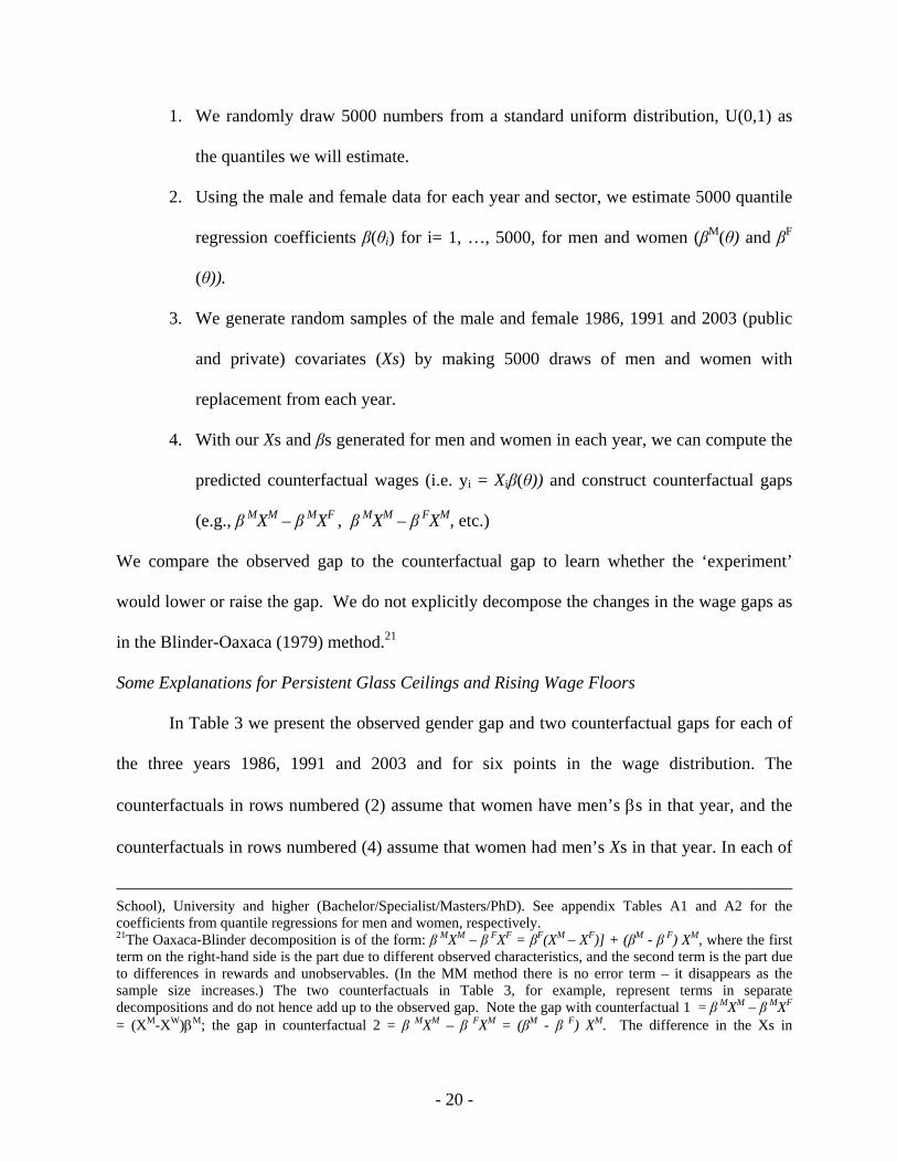
1. We randomly draw 5000 numbers from a standard uniform distribution, U(0,1) as

the quantiles we will estimate.

2. Using the male and female data for each year and sector, we estimate 5000 quantile

regression coefficients β(θi) for i= 1, …, 5000, for men and women (βM(θ) and βF

(θ)).

3. We generate random samples of the male and female 1986, 1991 and 2003 (public

and private) covariates (Xs) by making 5000 draws of men and women with

replacement from each year.

4. With our Xs and βs generated for men and women in each year, we can compute the

predicted counterfactual wages (i.e. yi = Xiβ(θ)) and construct counterfactual gaps

(e.g., β MXM – β MXF , β MXM – β FXM, etc.)

We compare the observed gap to the counterfactual gap to learn whether the ‘experiment’

would lower or raise the gap. We do not explicitly decompose the changes in the wage gaps as

in the Blinder-Oaxaca (1979) method.21

Some Explanations for Persistent Glass Ceilings and Rising Wage Floors

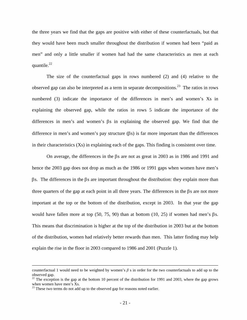
In Table 3 we present the observed gender gap and two counterfactual gaps for each of

the three years 1986, 1991 and 2003 and for six points in the wage distribution. The

counterfactuals in rows numbered (2) assume that women have men’s βs in that year, and the

counterfactuals in rows numbered (4) assume that women had men’s Xs in that year. In each of

School), University and higher (Bachelor/Specialist/Masters/PhD). See appendix Tables A1 and A2 for the coefficients from quantile regressions for men and women, respectively. 21The Oaxaca-Blinder decomposition is of the form: β MXM – β FXF = βF(XM – XF)] + (βM - β F) XM, where the first term on the right-hand side is the part due to different observed characteristics, and the second term is the part due to differences in rewards and unobservables. (In the MM method there is no error term – it disappears as the sample size increases.) The two counterfactuals in Table 3, for example, represent terms in separate decompositions and do not hence add up to the observed gap. Note the gap with counterfactual 1 = β MXM – β MXF = (XM-XW)βM; the gap in counterfactual 2 = β MXM – β FXM = (βM - β F) XM. The difference in the Xs in

- 21 -

the three years we find that the gaps are positive with either of these counterfactuals, but that

they would have been much smaller throughout the distribution if women had been “paid as

men” and only a little smaller if women had had the same characteristics as men at each

quantile.22

The size of the counterfactual gaps in rows numbered (2) and (4) relative to the

observed gap can also be interpreted as a term in separate decompositions.23 The ratios in rows

numbered (3) indicate the importance of the differences in men’s and women’s Xs in

explaining the observed gap, while the ratios in rows 5 indicate the importance of the

differences in men’s and women’s βs in explaining the observed gap. We find that the

difference in men’s and women’s pay structure (βs) is far more important than the differences

in their characteristics (Xs) in explaining each of the gaps. This finding is consistent over time.

On average, the differences in the βs are not as great in 2003 as in 1986 and 1991 and

hence the 2003 gap does not drop as much as the 1986 or 1991 gaps when women have men’s

βs. The differences in the βs are important throughout the distribution: they explain more than

three quarters of the gap at each point in all three years. The differences in the βs are not more

important at the top or the bottom of the distribution, except in 2003. In that year the gap

would have fallen more at top (50, 75, 90) than at bottom (10, 25) if women had men’s βs.

This means that discrimination is higher at the top of the distribution in 2003 but at the bottom

of the distribution, women had relatively better rewards than men. This latter finding may help

explain the rise in the floor in 2003 compared to 1986 and 2001 (Puzzle 1).

counterfactual 1 would need to be weighted by women’s β s in order for the two counterfactuals to add up to the observed gap. 22 The exception is the gap at the bottom 10 percent of the distribution for 1991 and 2003, where the gap grows when women have men’s Xs. 23 These two terms do not add up to the observed gap for reasons noted earlier.

- 22 -

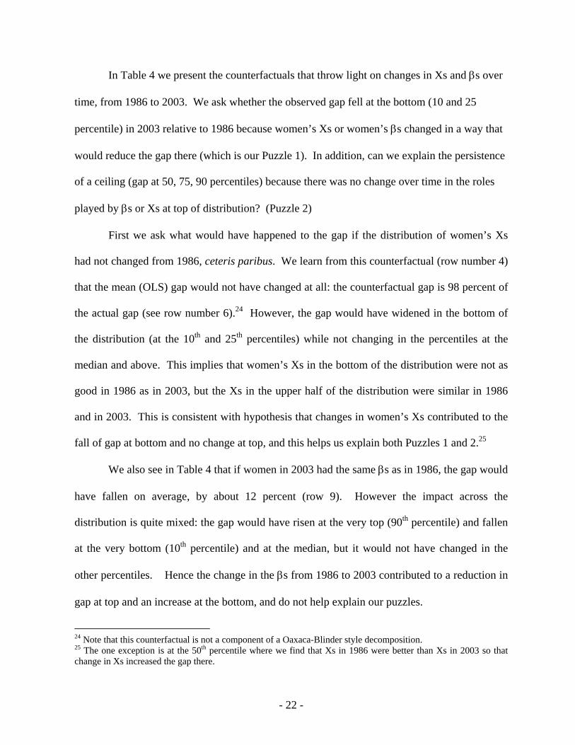
In Table 4 we present the counterfactuals that throw light on changes in Xs and βs over

time, from 1986 to 2003. We ask whether the observed gap fell at the bottom (10 and 25

percentile) in 2003 relative to 1986 because women’s Xs or women’s βs changed in a way that

would reduce the gap there (which is our Puzzle 1). In addition, can we explain the persistence

of a ceiling (gap at 50, 75, 90 percentiles) because there was no change over time in the roles

played by βs or Xs at top of distribution? (Puzzle 2)

First we ask what would have happened to the gap if the distribution of women’s Xs

had not changed from 1986, ceteris paribus. We learn from this counterfactual (row number 4)

that the mean (OLS) gap would not have changed at all: the counterfactual gap is 98 percent of

the actual gap (see row number 6).24 However, the gap would have widened in the bottom of

the distribution (at the 10th and 25th percentiles) while not changing in the percentiles at the

median and above. This implies that women’s Xs in the bottom of the distribution were not as

good in 1986 as in 2003, but the Xs in the upper half of the distribution were similar in 1986

and in 2003. This is consistent with hypothesis that changes in women’s Xs contributed to the

fall of gap at bottom and no change at top, and this helps us explain both Puzzles 1 and 2.25

We also see in Table 4 that if women in 2003 had the same βs as in 1986, the gap would

have fallen on average, by about 12 percent (row 9). However the impact across the

distribution is quite mixed: the gap would have risen at the very top (90th percentile) and fallen

at the very bottom (10th percentile) and at the median, but it would not have changed in the

other percentiles. Hence the change in the βs from 1986 to 2003 contributed to a reduction in

gap at top and an increase at the bottom, and do not help explain our puzzles.

24 Note that this counterfactual is not a component of a Oaxaca-Blinder style decomposition. 25 The one exception is at the 50th percentile where we find that Xs in 1986 were better than Xs in 2003 so that change in Xs increased the gap there.

- 23 -

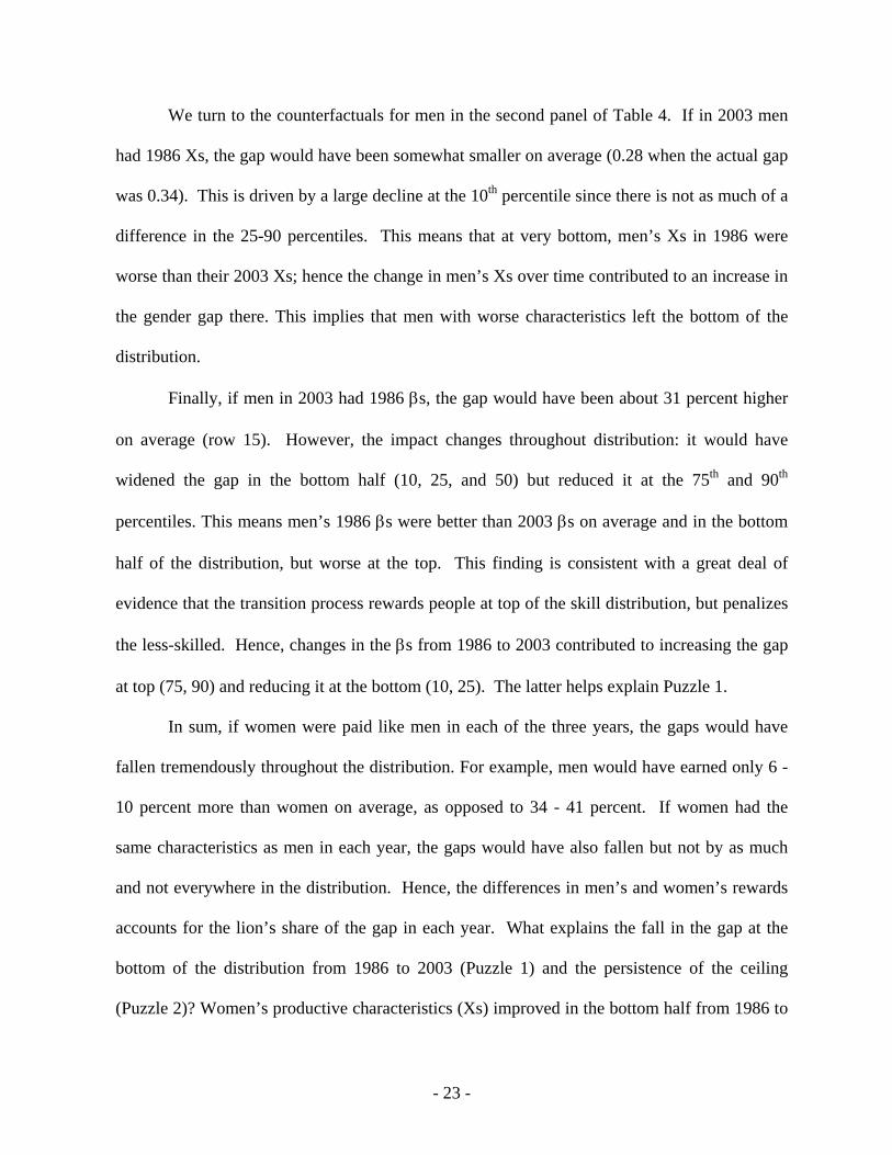
We turn to the counterfactuals for men in the second panel of Table 4. If in 2003 men

had 1986 Xs, the gap would have been somewhat smaller on average (0.28 when the actual gap

was 0.34). This is driven by a large decline at the 10th percentile since there is not as much of a

difference in the 25-90 percentiles. This means that at very bottom, men’s Xs in 1986 were

worse than their 2003 Xs; hence the change in men’s Xs over time contributed to an increase in

the gender gap there. This implies that men with worse characteristics left the bottom of the

distribution.

Finally, if men in 2003 had 1986 βs, the gap would have been about 31 percent higher

on average (row 15). However, the impact changes throughout distribution: it would have

widened the gap in the bottom half (10, 25, and 50) but reduced it at the 75th and 90th

percentiles. This means men’s 1986 βs were better than 2003 βs on average and in the bottom

half of the distribution, but worse at the top. This finding is consistent with a great deal of

evidence that the transition process rewards people at top of the skill distribution, but penalizes

the less-skilled. Hence, changes in the βs from 1986 to 2003 contributed to increasing the gap

at top (75, 90) and reducing it at the bottom (10, 25). The latter helps explain Puzzle 1.

In sum, if women were paid like men in each of the three years, the gaps would have

fallen tremendously throughout the distribution. For example, men would have earned only 6 -

10 percent more than women on average, as opposed to 34 - 41 percent. If women had the

same characteristics as men in each year, the gaps would have also fallen but not by as much

and not everywhere in the distribution. Hence, the differences in men’s and women’s rewards

accounts for the lion’s share of the gap in each year. What explains the fall in the gap at the

bottom of the distribution from 1986 to 2003 (Puzzle 1) and the persistence of the ceiling

(Puzzle 2)? Women’s productive characteristics (Xs) improved in the bottom half from 1986 to

- 24 -

2003 but stayed the same in the top of the distribution. The worsening of men’s pay structure

(βs) at the bottom half of the distribution also contributed to reducing the gaps there, as it

improved women’s relative position.

Public-Private Sectors: what explains the different ceilings?

We now turn to possible explanations for the third puzzle, why the gap is larger in the

public sector at the top of the distribution. This may result from bigger compositional

differences between men and women within each sector or it could also be due to a higher

degree of discrimination within one sector compared to the other (i.e., relative differences in

men’s and women’s βs in the two sectors).

In Table 5 we present the standard Blinder-Oaxaca type decompositions at different

points of the distribution of wages. In rows number (1) we show the raw gender gaps in the

public and private sectors: 0.30 and 0.26, respectively. The counterfactuals in rows numbered

(2) show the gap that would exist if women were rewarded with men’s pay structure in the

same sector, ceteris paribus; the counterfactuals in rows (4) show the gaps that would exist if

women had men’s characteristics in their same sector. Rows numbered (3) and (5) show both

the relative importance of the differences in men’s and women’s Xs and βs, respectively, in

explaining the gap and the relative effect of the counterfactual to the observed gap.26

In both the public and the private sector, the gender gap is mainly to be due to

differences in rewards. If women had men’s βs in the private sectors, the mean gap would have

fallen to nearly zero and it would have fallen more in the top half than in the bottom half of the

distribution. In the public sector, the mean gap would have also fallen, but not by as much:

26 As noted above with the similar exercise in Table 3, these two components do not add up exactly to the observed gap because we are looking at BM(XM-XF) and (BM-BF)XM, when the second term should be (BM-BF)XF in order for the two components to add up to the observed gap. We are more interested in seeing the gap with the women’s βs and Xs changed as they are in these counterfactuals, than in getting the decomposition to add up.

- 25 -

from 0.39 to 0.21. It would have fallen more in the top than in the bottom of the distribution,

like in the private sector. But in the private sector, the differences in rewards explain the entire

gender pay gap at the top: Note women would be paid more than men in the top half of the

distribution in the private sector if they were rewarded as men are in that sector.

There is not much difference between men’s and women’s characteristics on average,

and the size of the mean counterfactual and observed gaps in each sector are very similar for

each sector. However, at the bottom of the distribution (10 percentile), we see that women have

better characteristics than men, as the part of the gap explained by the βs is more than 100

percent. This is even more pronounced in the public sector, suggesting that women in the

bottom of the state pay scale have superior demographic characteristics that compensate them

for lower rewards (potentially discrimination). On the other hand, the composition effect is

different for the public and private sectors in the upper part of the distribution and it helps

explain why the ceiling is lower in the public than in the private sector (Puzzle 3). In the

private sector men’s Xs are worse than women’s at the 75th and 90th percentiles, whereas in the

public sector men’s Xs are somewhat better than women’s at the 75th and 90th percentiles.

Hence the larger gap in the top of the distribution (i.e., lower ceiling) in the public sector

compared to the private sector is partially explained by the differences in men’s and women’s

Xs in each sector, since women have relatively poorer characteristics in the public as compared

to the private sector.

7. Another explanation for the rise in the floor from 1986/91 to 2003

We discussed some changes in the institutions in Ukraine with the transition, and it is

difficult to assess their impact on the change in the gender gap with the counterfactual analysis

above. However, we know from our analysis of wage inequality in Ukraine (Ganguli and

- 26 -

Terrell, 2005) that kernel density estimates for men’s and women’s wages in 1986 and 2003

show that the minimum wage is binding for women in both years, but became especially

important in 2003. In Figure 3 we add estimates for the distribution of men’s and women’s

wages those kernel density estimates in 1991 in Figure 3. Moreover, in Figure 4 we present

kernel density estimates for men’s and women’s wages in the private and public sectors in

2003. These figures clearly show the importance of the minimum wage for women in each of

these three years. There is a clear spike in the women’s distribution of wages at a point that

represents the minimum wage in that year. 27 The density at the spike around the minimum

wage rises from about 0.8 in 1986 to 1.5 in 2003. It seems as if the women’s wage distribution

collapses around the minimum wage in 2003. From Figure 4, it is clear that it is the public

sector which is employing most of its female workforce at that wage. The density at the

minimum wage is much lower in the private sector. Hence, the decline in the gap at the bottom

of the distribution from 1986/1991 to 2003 may have to do with better compliance with and/or

a higher level of the minimum wage and this is affecting women more over time.

8. Conclusion

In this paper, we set out to analyze Ukraine’s gender wage gap during communism and

during the transition to a market economy, as the country moves toward Europe. We find that

the raw mean gender gap remained about the same from 1986 to 1991 (0.40 and 0.41,

respectively) but declined in 2003 to 0.34. The 1991 to 2003 decline in the average gap is the

result of a decline in the gaps in the lower part of the distribution, indicating a stronger floor for

women in 2003. We find evidence that a ‘glass ceiling’ (in a loose sense) exists and is

27 The minimum wages in 1986 and 2003 are taken from Minimum Wage decrees. However, the minimum wage in 1991 is our best estimate as to what it was in that year, given that we know the minimum was raised from 70 to 80 rubles from 1976 to 1985. By process of interpolation, we expect it to be about 90 rubles in 1991.

- 27 -

persistent in all three years, in that the gap in the upper half of the distribution is larger than in

the lower half. Most notably, we find that mean gap is larger in the public sector and that the

glass ceiling is lower in the public sector than in the private sector, which is counter to other

studies. A comparison with estimates for eleven European countries indicates that the mean

gender gap in the public sector is much higher while the gap in the private sector is at similar

levels to these European countries.

We find that a difference in rewards, often interpreted as discrimination, is the most

important factor explaining the gender gap, at the mean and throughout the distribution. We

attribute the persistence of the glass ceiling from Soviet times throughout the transition period

to continued discrimination and little change in the relative characteristics of men and women

at the top. The drop in the gap at the bottom of the distribution in 2003 appears to be a result of

the minimum wage raising the wage floor for women over time, as well as to composition

effects, with women’s characteristics compensating them for the discrimination (poorer set of

wages) they may face. However, there is also evidence that a worsening in the men’s reward

structure at the bottom of the distribution also contributes to a decline in the gap there. We also

find that the lower glass ceiling in the public sector compared to the private sector is a result of

differential composition of men and women; i.e., women’s characteristics in this sector are not

as good as men’s when compared to the relative characteristics of men and women in the

private sector.

It is clear that the gender wage gap will be an important measure of gender equality in

Ukraine in the coming years as it begins its bid to join the European Union. Our findings

suggest that if the new government wants to implement gender equal policies, it should start re-

evaluating the system of compensation in the public sector and recognizing the incidence of

- 28 -

discrimination there. With the glass ceiling being more prevalent in the public sector than in

the growing private sector, the Government must recognize that it should be a model as a

gender equal employer. If it were to eliminate the gaps in the public sector, or at least reduce

them to the current levels in the private sector, Ukraine’s gender wage gaps would be on par

with the European Union.

- 29 -

References

Albrecht, James, Anders Bjoekland, and Susan Vroman, 2003. “Is There a Glass Ceiling in Sweden?” Journal of Labor Economics, 21(1): 145 – 177.

Anderson, Kathryn and Richard Pomfret, 2003. “Women in the Labour Market in the Kyrgyz

Republic, 1993 and 1997,” in Anderson, K. and R. Pomfret, eds. Consequences of Creating a Market Economy: Evidence from Household Surveys in Central Asia. Edward Elgar, Cheltenham, UK.

Arulampalam, Wiji, Alison Booth, and Mark Bryan, 2005. “Is there a glass ceiling over

Europe? Exploring the Gender Pay Gap across the Wage Distribution,” unpublished paper University of Warwick, April 30.

Blau, Francine and Lawrence Kahn, 2003. “Understanding International Differences in the

Gender Pay Gap,” Journal of Labor Economics, 21(1): 106-144. ________, 1996. “Wage Structure and Gender Earnings Differentials: An International

Comparison,” Economica, Supplement: Economic Policy and Income Distribution, 63(250): S29-S62.

Blinder, Alan S., 1973. “Wage Discrimination: Reduced Form and Structural Variables,”

Journal of Human Resources, Vol 8: 436-455. Brainerd, Elizabeth, 2002. “Five Years After: The Impact of Mass Privatization on Wages in

Russia, 1993-1998,” Journal of Comparative Economics, Vol. 30, No. 1, March: 160-190.

________, 2000. “Women in Transition: Changes in Gender Wage Differentials in Eastern

Europe and the Former Soviet Union,” Industrial and Labor Relations Review, Vol. 54, No. 1, October: 138-162.

Buchinsky, Moshe, 1998. “Recent Advances in Quantile Regression Models: A Practical

Guideline for Empirical Research,” The Journal of Human Resources, No. 33: 88-126. De la Rica, Sara, Juan J. Dolado, Vanesa Llorens, 2005 “Ceiling and Floors: Gender Wage

Gaps by Education in Spain,” IZA Discussion Paper No. 1483. DiNardo, John, Nicole Fortin, and Thomas Lemieux, 1996. “Labor Market Institutions and the

Distribution of Wages, 1973-1992: A Semiparametric Approach,” Econometrica, Vol. 64, No. 5: 1001-1044.

Elborgh-Woytek, Katrin and Mark Lewis, 2002. “Privatization in Ukraine: Challenges of

Assessment and Coverage in Fund Conditionality,” IMF Policy Discussion Paper PDP/02/7, May.

- 30 -

Ganguli, Ina and Katherine Terrell, 2005. “Institutions, Markets and Men’s and Women’s Wage Inequality: Evidence from Ukraine,” IZA Discussion Paper 1724.

Gorodnichenko Yuriy and Klara Sabirianova Peter, 2004. “Returns to schooling in Russia and

Ukraine: A Semiparametric Approach to Cross-Country Comparative Analysis,” Journal of Comparative Economics, Vol. 33: 324-350.

Human Rights Watch, 2003. “Women’s Work: Discrimination Against Women in the

Ukrainian Labor Force.” Human Rights Watch, Vol. 15, No. 5(D), August 2003. Hunt, Jennifer, 2002. “The Transition in East Germany: When is a Ten-Point Fall in the

Gender Wage Gap Bad News?” Journal of Labor Economics, Vol. 20, No. 1: 148-169. Jolliffe, Dean, 2002. “The Gender Wage Gap in Bulgaria: A Semiparametric Estimation of

Discrimination,” Journal of Comparative Economics, Vol. 30, No. 2: 276-295. Jolliffe, Dean and Nauro F. Campos, 2005. “Does market liberalization reduce gender

discrimination? Econometric evidence from Hungary, 1986-1998,” Labour Economics, Vol. 12, No. 1: 1-22.

Jurajda, Stepan, 2003. “Gender Wage Gap and Segregation in Enterprises and the Public

Sector in Late Transition Countries,” Journal of Comparative Economics, Vol. 31, No. 2: 199-222.

Koenker, Roger and Gilbert Bassett, 1978. “Regression Quantiles,” Econometrica, No. 46: 33-

50. Liu, Amy P., W. Meng, et al. 2000. “Sectoral Wage Differentials and Discrmimination in

Transitional China,” Journal of Population Economics, Vol. 13, No. 2: 331-352. Machado, José A. F. and José Mata, 2004. "Counterfactual Decomposition of Changes in

Wage Distributions using Quantile Regression," Journal of Applied Econometrics, Vol. …

Minnesota Advocates for Human Rights, 2005. “Stop Violence Against Women website.” At the following website visited Aug. 24, 2005: www.stopvaw.org/ukraine

Münich, Daniel, Jan Svejnar and Katherine Terrell, 2005a. “Is Women’s Human Capital

Valued more by Markets than by Planners?” Journal of Comparative Economic, Vol. 33, No. 2:278-299.

__________, 2005b. “Returns to Human Capital under the Communist Wage Grid and during

the Transition to a Market Economy,” Review of Economics and Statistics, Vol. 87, No. 1: 100-123.

- 31 -

Newell, Andrew and Barry Reilly, 2001. “The Gender Pay Gap in the Transition from Communism: Some Empirical Evidence,” Institute for the Study of Labor (IZA), Discussion Paper No. 268, March.

Newell, Andrew and Barry Reilly, 1996. “The Gender Wage Gap in Russia: Some Empirical

Evidence,” Labour Economics, Vol. 3, No. 5: 337-356. Oaxaca, Ronald, 1973. “Male-Female Wage Differentials in Urban Labor Markets,”

International Economic Review, Vol. 14, No. 3, October: 693-709. Ogloblin, Constantin G., 1999. “The Gender Earnings Differential in the Russian Transition

Economy,” Industrial and Labor Relations Review, Vol. 52, No. 4, July: 602-627. Orazem, Peter F., and Vodopivec, Milan, 1995. “Winners and Losers in the Transition:

Returns Education, Experience, and Gender in Slovenia,” The World Bank Economic Review, 9(2): 201-230.

Tansel, Aysit, 2004. “Public-Private Employment Choice, Wage Differentials and Gender in

Turkey,” IZA Discussion Paper No. 1262. Weichselbaumer, Doris and Rudolf Winter-Ebmer, 2003. “The Effects of Competition and

Equal Treatment Laws on the Gender Wage Differential,” IZA Discussion Paper No. 822.

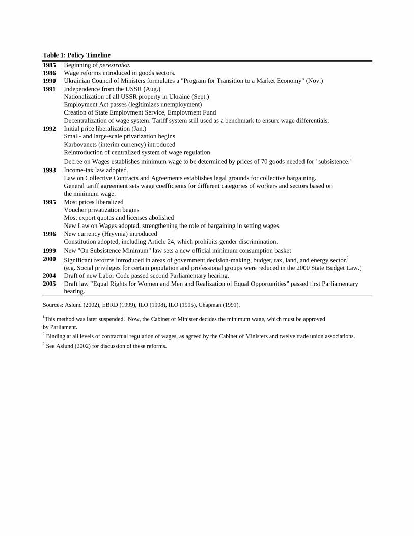
Table 1: Policy Timeline 1985 Beginning of perestroika.1986 Wage reforms introduced in goods sectors.1990 Ukrainian Council of Ministers formulates a "Program for Transition to a Market Economy" (Nov.)1991 Independence from the USSR (Aug.)

Nationalization of all USSR property in Ukraine (Sept.)Employment Act passes (legitimizes unemployment)Creation of State Employment Service, Employment FundDecentralization of wage system. Tariff system still used as a benchmark to ensure wage differentials.

1992 Initial price liberalization (Jan.) Small- and large-scale privatization beginsKarbovanets (interim currency) introducedReintroduction of centralized system of wage regulationDecree on Wages establishes minimum wage to be determined by prices of 70 goods needed for ' subsistence.'1

1993 Income-tax law adopted.Law on Collective Contracts and Agreements establishes legal grounds for collective bargaining.General tariff agreement sets wage coefficients for different categories of workers and sectors based on the minimum wage.

1995 Most prices liberalizedVoucher privatization beginsMost export quotas and licenses abolishedNew Law on Wages adopted, strengthening the role of bargaining in setting wages.

1996 New currency (Hryvnia) introducedConstitution adopted, including Article 24, which prohibits gender discrimination.

1999 New "On Subsistence Minimum" law sets a new official minimum consumption basket2000 Significant reforms introduced in areas of government decision-making, budget, tax, land, and energy sector.2

(e.g. Social privileges for certain population and professional groups were reduced in the 2000 State Budget Law.)2004 Draft of new Labor Code passed second Parliamentary hearing.2005 Draft law “Equal Rights for Women and Men and Realization of Equal Opportunities” passed first Parliamentary

hearing.

Sources: Aslund (2002), EBRD (1999), ILO (1998), ILO (1995), Chapman (1991).

1This method was later suspended. Now, the Cabinet of Minister decides the minimum wage, which must be approved by Parliament.2 Binding at all levels of contractual regulation of wages, as agreed by the Cabinet of Ministers and twelve trade union associations.2 See Aslund (2002) for discussion of these reforms.

Table2: Percentage Point Differences in Men's and Women's Labor Force Composition in Each Year

TOTAL PUBLIC PRIVATEMen-Women Men-Women Men-Women

86 91 03 03 03Age15-19 -1.3 -2.1 1.4 0.9 1.820-29 8.3 4.9 7.8 6.4 8.230-39 0.7 1.0 -1.3 1.7 -4.840-49 -6.1 -1.5 -6.5 -7.6 -5.250-56 -1.7 -2.3 -1.5 -1.5 0.0Education LevelsLess than High School -4.6 -2.5 2.2 0.3 4.2High School 1.1 -0.3 4.2 3.4 2.6Vocational 13.3 10.9 11.3 16.4 5.8Secondary Professional -8.6 -8.1 -11.4 -14.1 -7.5Higher Education -1.3 0.0 -6.3 -6.0 -5.0Nationality Ukrainian 0.6 1.0 -0.5 -1.1 -0.3Russian -0.9 -0.7 -0.8 0.6 -1.9

Other (Including Belorussian, Jewish)0.4 -0.3 1.4 0.5 2.2

Location %Kyiv 0.1 0.5 -1.5 -1.5 -2.6%Other -0.1 -0.5 1.5 1.5 2.6Activity of Enterprise%Agriculture, Hunting & Forestry 4.8 2.6 3.3 3.2 1.6%Manufacturing & Mining 8.2 6.1 11.6 15.0 2.8%Elec, Gas, Water & Construction 4.9 6.1 10.2 10.3 10.3%Transport, Communic. & Financial 2 -1.6 2.1 1.4 8.5 -10.5%Public Admin. & Defense 2.4 1.6 1.6 4.7 0.3 %Education, Health & Social Work -17.3 -17.0 -25.4 -40.0 -1.3%Other3 -1.4 -1.4 -2.8 -1.6 -3.2Ownership Type% Public 0.6 -2.4 -12.5 n.a n.a% Cooperative -0.6 0.9 0.1 n.a -0.4%DeNovo (incl Self-Emp) 0.1 1.5 5.7 n.a -0.6% Privatized -0.1 0.0 6.8 n.a 0.9

1 Includes Wholesale/Retail Trade, Repair of Motor Vehicles/Motorcycles; Hotels & Restaurants; Transport, Storage & Communication; Financial Intermediation, Real Estate, Renting & Business Activities.2 Includes Other Community, Social and Personal Service Activities.Note: Using sample weights.

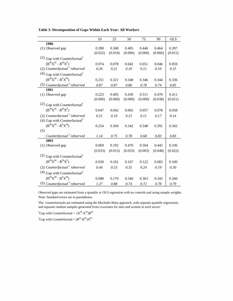
Table 3: Decomposition of Gaps Within Each Year: All Workers

10 25 50 75 90 OLS1986

(1) Observed gap 0.288 0.368 0.405 0.446 0.464 0.397(0.022) (0.019) (0.000) (0.000) (0.060) (0.015)

(2) Gap with Counterfactual1

(BMXM - BMXF) 0.074 0.078 0.042 0.051 0.046 0.059(3) Counterfactual 1 /observed 0.26 0.21 0.10 0.11 0.10 0.15(4) Gap with Counterfactual2

(BMXM - BFXM) 0.251 0.321 0.348 0.346 0.344 0.336(5) Counterfactual 2 /observed 0.87 0.87 0.86 0.78 0.74 0.85

1991(1) Observed gap 0.223 0.405 0.439 0.511 0.470 0.411

(0.000) (0.000) (0.000) (0.000) (0.038) (0.021)(2) Gap with Counterfactual1

(BMXM - BMXF) 0.047 0.042 0.065 0.057 0.078 0.058(3) Counterfactual 1 /observed 0.21 0.10 0.15 0.11 0.17 0.14(4) Gap with Counterfactual2

(BMXM - BFXM) 0.254 0.304 0.342 0.348 0.391 0.343(5)

Counterfactual 2 /observed 1.14 0.75 0.78 0.68 0.83 0.832003

(1) Observed gap 0.069 0.192 0.470 0.504 0.442 0.336(0.033) (0.013) (0.033) (0.003) (0.048) (0.022)

(2) Gap with Counterfactual1

(BMXM - BMXF) 0.030 0.101 0.167 0.122 0.083 0.100(3) Counterfactual 1 /observed 0.44 0.53 0.35 0.24 0.19 0.30(4) Gap with Counterfactual2

(BMXM - BFXM) 0.088 0.170 0.346 0.363 0.343 0.266(5) Counterfactual 2 /observed 1.27 0.88 0.74 0.72 0.78 0.79

Observed gaps are estimated from a quantile or OLS regression with no controls and using sample weights. Note: Standard errors are in parentheses.

The counterfactuals are estimated using the Machado-Mata approach, with separate quantile regressions and separate random samples generated from covariates for men and women in each sector:1Gap with Counterfactual = (XM-XW)BM

2Gap with Counterfactual = (BM-BW)XM

Table 4: Decomposition of Gaps Across Time, 1986 and 2003: All Workers

Gap 10 25 50 75 90 OLS(1) Observed in 1986 0.288 0.368 0.405 0.446 0.464 0.397

(0.022) (0.019) (0.000) (0.000) (0.060) (0.015)

(2) Observed in 2003 0.069 0.192 0.470 0.504 0.442 0.336(0.033) (0.013) (0.033) (0.003) (0.048) (0.022)

(3) Observed '03/ Observed '86 0.240 0.523 1.159 1.130 0.952 0.847

Counterfactuals for Women:(4) Gap with Counterfactual1

(BM03XM03 - BF03XF86) 0.112 0.223 0.415 0.460 0.431 0.328(5) Counterfactual1/Obs. '86 0.389 0.605 1.024 1.031 0.928 0.827(6) (5)/(3) 1.620 1.157 0.884 0.913 0.975 0.976(7) Gap with Counterfactual2

(BM03XM03 - BF86XF03) 0.054 0.182 0.365 0.467 0.497 0.295(8) Counterfactual2/Observed '86 0.189 0.495 0.900 1.047 1.071 0.744(9) (8)/(3) 0.787 0.947 0.777 0.927 1.125 0.878

Counterfactuals for Men:(10) Gap with Counterfactual3

(BM03XM86 - BF03XF03) 0.031 0.174 0.371 0.440 0.418 0.282(11) Counterfactual3/Observed '86 0.109 0.472 0.915 0.986 0.900 0.709(12) (11)/(3) 0.456 0.903 0.789 0.873 0.945 0.838(13) Gap with Counterfactual4

(BM86XM03 - BF03XF03) 0.409 0.440 0.478 0.436 0.370 0.441(14) Counterfactual4/Observed '86 1.422 1.196 1.180 0.977 0.796 1.110(15) (14)/(3) 5.931 2.287 1.018 0.865 0.836 1.311

Observed gaps are stimated from a quantile or OLS regression with no controls and using sample weight. Standard errors are in parentheses.The following counterfactuals are estimated using the Machado-Mata approach, with separate quantile regressions and separate random samples generated from covariates for men and women in each sector:1If women in 03 had Xs of women in 862If women in 03 had Bs of women in 863If men in 03 had Xs of men in 864If men in 03 had same Bs of men in 86

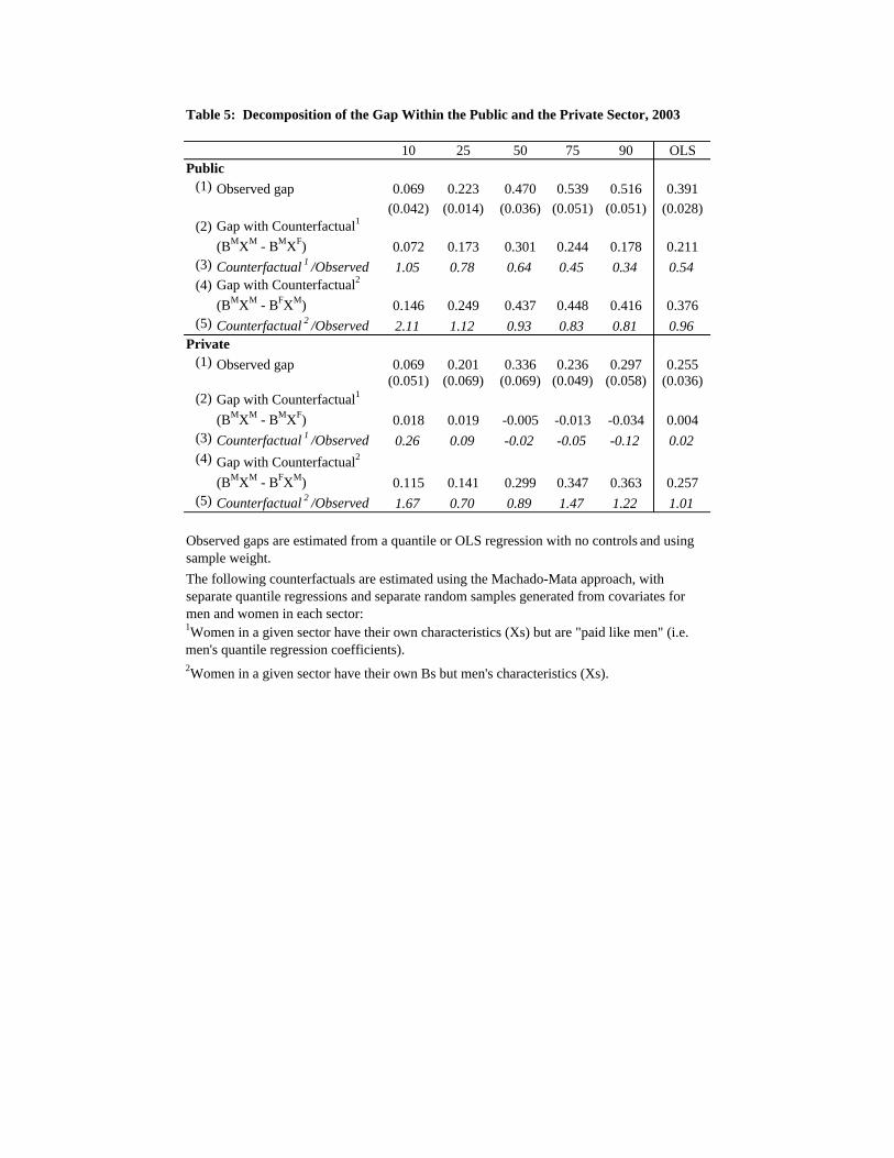
Table 5: Decomposition of the Gap Within the Public and the Private Sector, 2003

10 25 50 75 90 OLSPublic

(1) Observed gap 0.069 0.223 0.470 0.539 0.516 0.391(0.042) (0.014) (0.036) (0.051) (0.051) (0.028)

(2) Gap with Counterfactual1

(BMXM - BMXF) 0.072 0.173 0.301 0.244 0.178 0.211(3) Counterfactual 1 /Observed 1.05 0.78 0.64 0.45 0.34 0.54(4) Gap with Counterfactual2

(BMXM - BFXM) 0.146 0.249 0.437 0.448 0.416 0.376(5) Counterfactual 2 /Observed 2.11 1.12 0.93 0.83 0.81 0.96

Private(1) Observed gap 0.069 0.201 0.336 0.236 0.297 0.255

(0.051) (0.069) (0.069) (0.049) (0.058) (0.036)(2) Gap with Counterfactual1

(BMXM - BMXF) 0.018 0.019 -0.005 -0.013 -0.034 0.004(3) Counterfactual 1 /Observed 0.26 0.09 -0.02 -0.05 -0.12 0.02(4) Gap with Counterfactual2

(BMXM - BFXM) 0.115 0.141 0.299 0.347 0.363 0.257(5) Counterfactual 2 /Observed 1.67 0.70 0.89 1.47 1.22 1.01

Observed gaps are estimated from a quantile or OLS regression with no controls and using sample weight. The following counterfactuals are estimated using the Machado-Mata approach, with separate quantile regressions and separate random samples generated from covariates for men and women in each sector:1Women in a given sector have their own characteristics (Xs) but are "paid like men" (i.e. men's quantile regression coefficients).2Women in a given sector have their own Bs but men's characteristics (Xs).

Figure 1: Gender gaps Across the Distribution for 1986, 1991 and 2003

Note: Moving average over three percentiles

.1.2

.3.4

.5G

ap

0 10 20 30 40 50 60 70 80 90 100Percentile

2003 1991 1986

Gender Gap, 1986, 1991, 2003

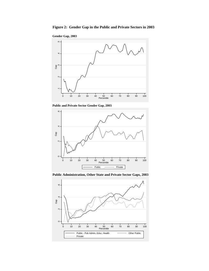
Figure 2: Gender Gap in the Public and Private Sectors in 2003

Gender Gap, 2003

Public and Private Sector Gender Gap, 2003

Public Administration, Other State and Private Sector Gaps, 2003

0.2

.4.6

Gap

0 10 20 30 40 50 60 70 80 90 100Percentile

Public Private

.1.2

.3.4

.5G

ap

0 10 20 30 40 50 60 70 80 90 100Percentile

0.2

.4.6

Gap

0 10 20 30 40 50 60 70 80 90 100Percentile

Public - Pub Admin, Educ, Health Other Public Private

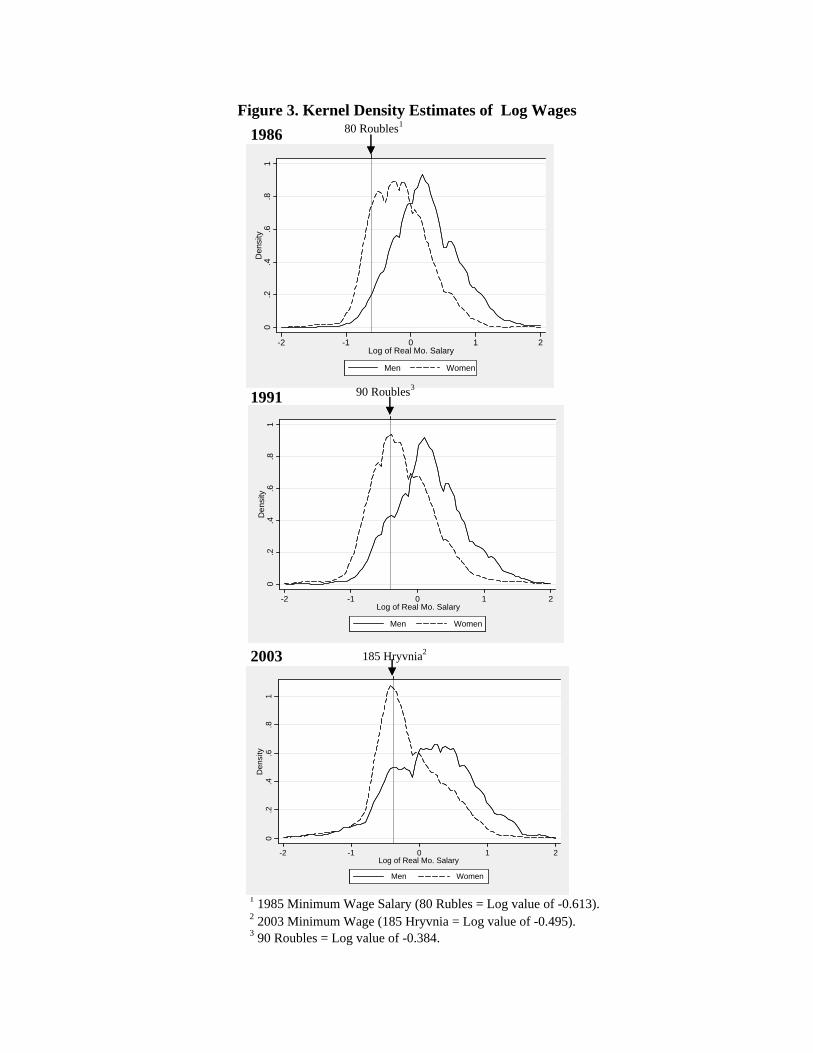
Figure 3. Kernel Density Estimates of Log Wages 1986

1991

2003

1 1985 Minimum Wage Salary (80 Rubles = Log value of -0.613). 2 2003 Minimum Wage (185 Hryvnia = Log value of -0.495).3 90 Roubles = Log value of -0.384.

0.2

.4.6

.81

Den

sity

-2 -1 0 1 2Log of Real Mo. Salary

Men Women

80 Roubles1

0.2

.4.6

.81

Den

sity

-2 -1 0 1 2Log of Real Mo. Salary

Men Women

185 Hryvnia2

0.2

.4.6

.81

Den

sity

-2 -1 0 1 2Log of Real Mo. Salary

Men Women

90 Roubles3

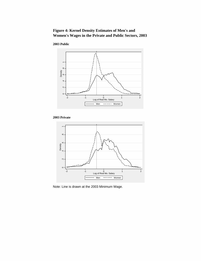
Figure 4: Kernel Density Estimates of Men's and Women's Wages in the Private and Public Sectors, 2003

2003 Public

2003 Private

Note: Line is drawn at the 2003 Minimum Wage.

0.2

.4.6

.81

Den

sity

-2 -1 0 1 2Log of Real Mo. Salary

Men Women

0.2

.4.6

.81

Den

sity

-2 -1 0 1 2Log of Real Mo. Salary

Men Women

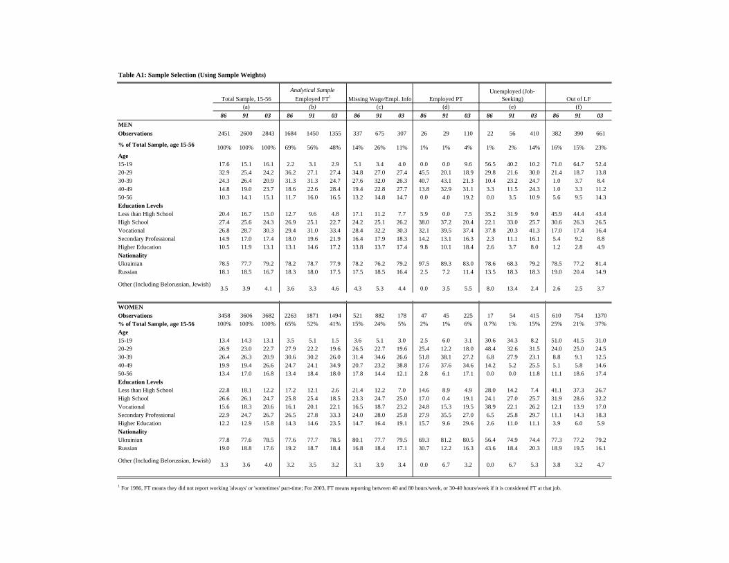
Table A1: Sample Selection (Using Sample Weights)

Total Sample, 15-56Analytical Sample

Employed FT1 Missing Wage/Empl. Info Employed PTUnemployed (Job-

Seeking) Out of LF(a) (b) (c) (d) (e) (f)

86 91 03 86 91 03 86 91 03 86 91 03 86 91 03 86 91 03MENObservations 2451 2600 2843 1684 1450 1355 337 675 307 26 29 110 22 56 410 382 390 661

% of Total Sample, age 15-56 100% 100% 100% 69% 56% 48% 14% 26% 11% 1% 1% 4% 1% 2% 14% 16% 15% 23%Age15-19 17.6 15.1 16.1 2.2 3.1 2.9 5.1 3.4 4.0 0.0 0.0 9.6 56.5 40.2 10.2 71.0 64.7 52.420-29 32.9 25.4 24.2 36.2 27.1 27.4 34.8 27.0 27.4 45.5 20.1 18.9 29.8 21.6 30.0 21.4 18.7 13.830-39 24.3 26.4 20.9 31.3 31.3 24.7 27.6 32.0 26.3 40.7 43.1 21.3 10.4 23.2 24.7 1.0 3.7 8.440-49 14.8 19.0 23.7 18.6 22.6 28.4 19.4 22.8 27.7 13.8 32.9 31.1 3.3 11.5 24.3 1.0 3.3 11.250-56 10.3 14.1 15.1 11.7 16.0 16.5 13.2 14.8 14.7 0.0 4.0 19.2 0.0 3.5 10.9 5.6 9.5 14.3Education LevelsLess than High School 20.4 16.7 15.0 12.7 9.6 4.8 17.1 11.2 7.7 5.9 0.0 7.5 35.2 31.9 9.0 45.9 44.4 43.4High School 27.4 25.6 24.3 26.9 25.1 22.7 24.2 25.1 26.2 38.0 37.2 20.4 22.1 33.0 25.7 30.6 26.3 26.5Vocational 26.8 28.7 30.3 29.4 31.0 33.4 28.4 32.2 30.3 32.1 39.5 37.4 37.8 20.3 41.3 17.0 17.4 16.4Secondary Professional 14.9 17.0 17.4 18.0 19.6 21.9 16.4 17.9 18.3 14.2 13.1 16.3 2.3 11.1 16.1 5.4 9.2 8.8Higher Education 10.5 11.9 13.1 13.1 14.6 17.2 13.8 13.7 17.4 9.8 10.1 18.4 2.6 3.7 8.0 1.2 2.8 4.9NationalityUkrainian 78.5 77.7 79.2 78.2 78.7 77.9 78.2 76.2 79.2 97.5 89.3 83.0 78.6 68.3 79.2 78.5 77.2 81.4Russian 18.1 18.5 16.7 18.3 18.0 17.5 17.5 18.5 16.4 2.5 7.2 11.4 13.5 18.3 18.3 19.0 20.4 14.9

Other (Including Belorussian, Jewish)3.5 3.9 4.1 3.6 3.3 4.6 4.3 5.3 4.4 0.0 3.5 5.5 8.0 13.4 2.4 2.6 2.5 3.7

WOMENObservations 3458 3606 3682 2263 1871 1494 521 882 178 47 45 225 17 54 415 610 754 1370% of Total Sample, age 15-56 100% 100% 100% 65% 52% 41% 15% 24% 5% 2% 1% 6% 0.7% 1% 15% 25% 21% 37%Age15-19 13.4 14.3 13.1 3.5 5.1 1.5 3.6 5.1 3.0 2.5 6.0 3.1 30.6 34.3 8.2 51.0 41.5 31.020-29 26.9 23.0 22.7 27.9 22.2 19.6 26.5 22.7 19.6 25.4 12.2 18.0 48.4 32.6 31.5 24.0 25.0 24.530-39 26.4 26.3 20.9 30.6 30.2 26.0 31.4 34.6 26.6 51.8 38.1 27.2 6.8 27.9 23.1 8.8 9.1 12.540-49 19.9 19.4 26.6 24.7 24.1 34.9 20.7 23.2 38.8 17.6 37.6 34.6 14.2 5.2 25.5 5.1 5.8 14.650-56 13.4 17.0 16.8 13.4 18.4 18.0 17.8 14.4 12.1 2.8 6.1 17.1 0.0 0.0 11.8 11.1 18.6 17.4Education LevelsLess than High School 22.8 18.1 12.2 17.2 12.1 2.6 21.4 12.2 7.0 14.6 8.9 4.9 28.0 14.2 7.4 41.1 37.3 26.7High School 26.6 26.1 24.7 25.8 25.4 18.5 23.3 24.7 25.0 17.0 0.4 19.1 24.1 27.0 25.7 31.9 28.6 32.2Vocational 15.6 18.3 20.6 16.1 20.1 22.1 16.5 18.7 23.2 24.8 15.3 19.5 38.9 22.1 26.2 12.1 13.9 17.0Secondary Professional 22.9 24.7 26.7 26.5 27.8 33.3 24.0 28.0 25.8 27.9 35.5 27.0 6.5 25.8 29.7 11.1 14.3 18.3Higher Education 12.2 12.9 15.8 14.3 14.6 23.5 14.7 16.4 19.1 15.7 9.6 29.6 2.6 11.0 11.1 3.9 6.0 5.9NationalityUkrainian 77.8 77.6 78.5 77.6 77.7 78.5 80.1 77.7 79.5 69.3 81.2 80.5 56.4 74.9 74.4 77.3 77.2 79.2Russian 19.0 18.8 17.6 19.2 18.7 18.4 16.8 18.4 17.1 30.7 12.2 16.3 43.6 18.4 20.3 18.9 19.5 16.1

Other (Including Belorussian, Jewish)3.3 3.6 4.0 3.2 3.5 3.2 3.1 3.9 3.4 0.0 6.7 3.2 0.0 6.7 5.3 3.8 3.2 4.7

1 For 1986, FT means they did not report working 'always' or 'sometimes' part-time; For 2003, FT means reporting between 40 and 80 hours/week, or 30-40 hours/week if it is considered FT at that job.

*

* * * * * * * * * *

* * * * * * * * * * * * *

Table A2: OLS & Quantile Regressions: Men

1986 1991 2003OLS 10 25 50 75 90 95 OLS 10 25 50 75 90 95 OLS 10 25 50 75 90 95

Nationality (Ukrainian omitted) Russian 0.089** 0.011 0.094** 0.076* 0.091* 0.150* 0.085 0.169** 0.123* 0.169** 0.136** 0.126** 0.034 0.313* 0.046 -0.019 -0.015 0.085 0.092 0.132 0.018

(0.029) (0.067) (0.030) (0.035) (0.035) (0.067) (0.109) (0.040) (0.060) (0.041) (0.034) (0.044) (0.079) (0.131) (0.040) (0.074) (0.058) (0.045) (0.065) (0.075) (0.079)

Other (inc. Byelorussian, Jewish)-0.066 -0.009 -0.070 -0.116 -0.181* -0.213 -0.052 0.131 0.285** 0.085 0.009 0.068 0.072 0.445* 0.115 -0.022 -0.075 0.131 0.123 0.525** 0.437**(0.061) (0.139) (0.065) (0.072) (0.069) (0.130) (0.197) (0.090) (0.100) (0.093) (0.075) (0.094) (0.154) (0.225) (0.073) (0.127) (0.106) (0.086) (0.113) (0.149) (0.139)

Education (Less than HS omitted)High School 0.045 -0.013 0.093* 0.079 -0.008 0.069 0.069 -0.005 -0.016 0.035 -0.005 -0.016 -0.065 0.066 0.009 0.151 0.009 0.043 0.053 0.095 -0.273

(0.042) (0.094) (0.040) (0.049) (0.050) (0.094) (0.165) (0.062) (0.093) (0.065) (0.053) (0.069) (0.124) (0.155) (0.077) (0.137) (0.110) (0.086) (0.121) (0.156) (0.145)Vocational 0.112** 0.060 0.101** 0.174** 0.089 0.149 0.255 0.051 0.065 0.056 0.056 0.016 0.101 0.234 0.042 0.180 0.040 0.112 0.068 0.128 -0.221

(0.041) (0.090) (0.038) (0.048) (0.048) (0.093) (0.163) (0.061) (0.089) (0.062) (0.051) (0.068) (0.122) (0.149) (0.075) (0.131) (0.106) (0.084) (0.116) (0.152) (0.138)Secondary Professional 0.191** 0.189 0.225** 0.251** 0.172** 0.128 0.209 0.247** 0.145 0.155* 0.197** 0.180* 0.402** 0.451** 0.183* 0.286* 0.186 0.261** 0.205 0.262 -0.015

(0.044) (0.097) (0.041) (0.052) (0.052) (0.099) (0.166) (0.064) (0.098) (0.066) (0.054) (0.072) (0.128) (0.164) (0.078) (0.135) (0.110) (0.088) (0.122) (0.158) (0.147)

Higher Ed (Bach, Spec, Masters, PhD) 0.239** 0.273** 0.350** 0.294** 0.139* 0.192 0.236 0.313** 0.298** 0.307** 0.288** 0.333** 0.349** 0.337 0.394** 0.442** 0.387** 0.464** 0.460** 0.557** 0.221(0.048) (0.106) (0.045) (0.055) (0.057) (0.103) (0.170) (0.069) (0.097) (0.069) (0.057) (0.075) (0.130) (0.177) (0.081) (0.140) (0.114) (0.090) (0.125) (0.160) (0.150)

Age 0.029** 0.015 0.014 0.033** 0.043** 0.024 0.039 0.039** 0.034* 0.038** 0.028** 0.043** 0.055** 0.029 0.036** 0.017 0.015 0.042** 0.049** 0.039 0.050*(0.009) (0.019) (0.009) (0.011) (0.010) (0.021) (0.035) (0.011) (0.017) (0.012) (0.009) (0.012) (0.021) (0.033) (0.011) (0.021) (0.016) (0.012) (0.018) (0.020) (0.022)

Age2 -0.000**-0.000 -0.000 -0.000* -0.001* -0.000 -0.000 -0.001* -0.000* -0.000* -0.000* -0.001* -0.001* -0.000 -0.000* -0.000 -0.000 -0.001* -0.001* -0.000 -0.001*(0.000) (0.000) (0.000) (0.000) (0.000) (0.000) (0.000) (0.000) (0.000) (0.000) (0.000) (0.000) (0.000) (0.000) (0.000) (0.000) (0.000) (0.000) (0.000) (0.000) (0.000)

Kyiv 0.103* 0.142 0.051 0.137* 0.130* 0.078 0.004 0.271** 0.080 0.054 0.091 0.168* 0.359** 1.826** 0.209** 0.004 0.143 0.344** 0.282** 0.207* 0.303*(0.047) (0.118) (0.053) (0.063) (0.061) (0.109) (0.139) (0.063) (0.104) (0.067) (0.057) (0.072) (0.123) (0.191) (0.055) (0.100) (0.090) (0.066) (0.092) (0.103) (0.122)

Activity of Enterprise (Agriculture is omitted)Manufacturing & Mining 0.395** 0.367** 0.407** 0.430** 0.466** 0.403** 0.354* 0.441** 0.352** 0.439** 0.442** 0.451** 0.449** 0.474** 0.740** 0.886** 0.725** 0.813** 0.582** 0.550** 0.313*

(0.032) (0.074) (0.033) (0.039) (0.041) (0.082) (0.155) (0.047) (0.075) (0.049) (0.039) (0.051) (0.093) (0.140) (0.054) (0.097) (0.078) (0.059) (0.088) (0.105) (0.122)

Electricity, Gas, Water & Construction0.250** 0.367** 0.235** 0.255** 0.172** 0.212* 0.195 0.306** 0.274** 0.312** 0.400** 0.295** 0.279* 0.236 0.649** 0.857** 0.547** 0.721** 0.554** 0.592** 0.253(0.044) (0.095) (0.045) (0.053) (0.055) (0.107) (0.195) (0.061) (0.097) (0.064) (0.051) (0.066) (0.119) (0.179) (0.062) (0.114) (0.090) (0.069) (0.099) (0.118) (0.132)

Transport, Communic. & Financial1 0.173** 0.284** 0.210** 0.243** 0.123** 0.063 -0.053 0.341** 0.235** 0.353** 0.314** 0.326** 0.251* 0.340* 0.654** 0.752** 0.598** 0.745** 0.545** 0.503** 0.249(0.038) (0.087) (0.040) (0.047) (0.047) (0.091) (0.167) (0.053) (0.085) (0.056) (0.045) (0.059) (0.107) (0.168) (0.057) (0.099) (0.082) (0.063) (0.093) (0.112) (0.130)

Public Administration & Defense0.294** 0.400** 0.308** 0.314** 0.294** 0.238 0.073 0.356** 0.304* 0.233** 0.230** 0.290** 0.372* 0.713** 0.688** 0.956** 0.615** 0.735** 0.543** 0.460** 0.072(0.053) (0.119) (0.057) (0.068) (0.070) (0.136) (0.220) (0.080) (0.126) (0.086) (0.070) (0.091) (0.164) (0.241) (0.080) (0.146) (0.118) (0.091) (0.128) (0.153) (0.161)

Education, Health, & Social Work-0.131* -0.059 -0.131* -0.128 -0.070 -0.184 -0.256 -0.032 -0.026 0.009 -0.083 -0.077 -0.151 -0.180 0.113 0.534** 0.221* 0.091 -0.149 -0.223 -0.483**(0.054) (0.136) (0.056) (0.066) (0.068) (0.115) (0.171) (0.076) (0.110) (0.077) (0.065) (0.081) (0.137) (0.224) (0.073) (0.144) (0.107) (0.082) (0.120) (0.139) (0.159)

Other2 0.042 0.149 0.067 0.081 -0.012 -0.079 -0.231 0.231** -0.081 0.130 0.193** 0.297** 0.172 0.205 0.357** 0.615** 0.354** 0.416** 0.221 0.163 -0.150(0.055) (0.123) (0.056) (0.069) (0.070) (0.117) (0.211) (0.079) (0.112) (0.083) (0.067) (0.085) (0.139) (0.238) (0.077) (0.132) (0.106) (0.084) (0.118) (0.135) (0.151)

Constant -0.649**-0.857* -0.699* -0.841* -0.597* -0.017 -0.109 -0.922* -1.354* -1.232* -0.797* -0.722* -0.560 -0.039 -1.159* -1.779* -1.063* -1.384* -0.935* -0.565 0.051(0.150) (0.351) (0.169) (0.195) (0.184) (0.391) (0.690) (0.191) (0.294) (0.218) (0.168) (0.221) (0.388) (0.542) (0.202) (0.395) (0.297) (0.228) (0.327) (0.351) (0.391)

N = 1666 1666 1666 1666 1666 1666 1666 1430 1430 1430 1430 1430 1430 1430 1340 1340 1340 1340 1340 1340 1340R-Squared = 0.17 0.15 0.23* significant at 5%; ** significant at 1%.1 Includes Wholesale/Retail Trade, Repair of Motor Vehicles/Motorcycles; Hotels & Restaurants; Transport, Storage & Communication; Financial Intermediation, Real Estate, Renting & Business Activities.

* * * * * * * *

* * * * * * * * * * * *

Table A3: OLS & Quantile Regressions: Women

1986 1991 2003OLS 10 25 50 75 90 95 OLS 10 25 50 75 90 95 OLS 10 25 50 75 90 95

Nationality (Ukrainian omitted) Russian 0.027 0.072** 0.051** 0.025 -0.001 -0.045 -0.091 0.056 0.079** 0.042 0.091** 0.105** 0.018 0.029 0.130** 0.054 0.075** 0.113** 0.146** 0.141* 0.063

(0.023) (0.025) (0.012) (0.019) (0.026) (0.039) (0.064) (0.031) (0.029) (0.024) (0.032) (0.025) (0.056) (0.096) (0.034) (0.045) (0.025) (0.032) (0.036) (0.064) (0.096)

Other (inc. Byelorussian, Jewish)0.015 -0.002 0.000 -0.003 -0.064 0.084 0.134 0.050 0.054 -0.025 -0.025 -0.000 -0.128 0.528** 0.001 0.165 0.105* 0.038 0.102 -0.077 -0.108(0.050) (0.050) (0.024) (0.041) (0.058) (0.080) (0.148) (0.066) (0.056) (0.046) (0.067) (0.050) (0.123) (0.134) (0.073) (0.087) (0.052) (0.067) (0.077) (0.124) (0.167)

Education (Less than HS omitted)High School 0.078** 0.109** 0.022 0.109** 0.088** 0.017 0.014 0.071 0.079* 0.038 0.099* 0.092** 0.030 -0.105 0.188* 0.050 0.120* 0.227** 0.125 0.239 0.220

(0.030) (0.030) (0.014) (0.025) (0.033) (0.049) (0.082) (0.044) (0.036) (0.032) (0.044) (0.033) (0.074) (0.125) (0.086) (0.104) (0.060) (0.080) (0.089) (0.142) (0.139)Vocational 0.133** 0.133** 0.093** 0.188** 0.128** 0.064 0.111 0.143** 0.076 0.093** 0.150** 0.120** 0.179* 0.069 0.201* -0.002 0.121* 0.246** 0.134 0.277* 0.269

(0.034) (0.034) (0.017) (0.029) (0.039) (0.056) (0.093) (0.048) (0.039) (0.035) (0.049) (0.037) (0.084) (0.139) (0.085) (0.104) (0.059) (0.079) (0.088) (0.141) (0.138)Secondary Professional 0.133** 0.174** 0.132** 0.213** 0.096** 0.080 0.083 0.178** 0.219** 0.194** 0.198** 0.125** 0.089 0.038 0.281** 0.096 0.153** 0.316** 0.222* 0.403** 0.375**

(0.030) (0.032) (0.015) (0.025) (0.033) (0.051) (0.087) (0.045) (0.036) (0.032) (0.044) (0.034) (0.074) (0.124) (0.084) (0.100) (0.058) (0.078) (0.087) (0.140) (0.129)

Higher Ed (Bach, Spec, Masters, PhD) 0.394** 0.398** 0.415** 0.473** 0.481** 0.447** 0.374** 0.460** 0.371** 0.422** 0.494** 0.503** 0.490** 0.378** 0.523** 0.241* 0.376** 0.614** 0.533** 0.723** 0.794**(0.035) (0.038) (0.017) (0.029) (0.038) (0.057) (0.095) (0.050) (0.043) (0.037) (0.050) (0.038) (0.084) (0.135) (0.085) (0.102) (0.059) (0.079) (0.089) (0.141) (0.136)

Age 0.009 0.002 0.005 0.015* 0.010 -0.001 -0.018 -0.002 0.023** 0.000 0.004 -0.008 -0.024 -0.033 0.012 0.030* 0.007 0.007 0.004 0.004 -0.006(0.007) (0.008) (0.003) (0.006) (0.008) (0.011) (0.019) (0.008) (0.008) (0.006) (0.009) (0.008) (0.017) (0.028) (0.010) (0.012) (0.008) (0.010) (0.011) (0.018) (0.026)

Age2 -0.000 -0.000 -0.000 -0.000* -0.000 0.000 0.000 0.000 -0.000* 0.000 -0.000 0.000 0.000 0.000 -0.000 -0.000* -0.000 -0.000 -0.000 -0.000 0.000(0.000) (0.000) (0.000) (0.000) (0.000) (0.000) (0.000) (0.000) (0.000) (0.000) (0.000) (0.000) (0.000) (0.000) (0.000) (0.000) (0.000) (0.000) (0.000) (0.000) (0.000)

Kyiv 0.116** 0.109** 0.117** 0.117** 0.077 0.079 0.074 0.355** 0.112** 0.094* 0.085 0.207** 0.661** 1.958** 0.296** 0.110 0.136** 0.278** 0.371** 0.354** 0.486**(0.037) (0.038) (0.019) (0.033) (0.046) (0.074) (0.116) (0.050) (0.040) (0.037) (0.055) (0.044) (0.099) (0.161) (0.044) (0.058) (0.034) (0.044) (0.051) (0.089) (0.126)

Activity of Enterprise (Agriculture is omitted)Manufacturing & Mining 0.246** 0.181** 0.208** 0.277** 0.208** 0.270** 0.344** 0.251** 0.197** 0.223** 0.300** 0.221** 0.290** 0.344** 0.362** 0.831** 0.360** 0.269** 0.440** 0.187 -0.059

(0.030) (0.033) (0.015) (0.025) (0.034) (0.051) (0.084) (0.042) (0.041) (0.032) (0.044) (0.035) (0.074) (0.124) (0.056) (0.070) (0.043) (0.053) (0.061) (0.108) (0.157)

Electricity, Gas, Water & Construction0.239** 0.188** 0.233** 0.202** 0.209** 0.248** 0.321** 0.254** 0.321** 0.227** 0.279** 0.223** 0.392** 0.339 0.444** 1.023** 0.411** 0.382** 0.474** 0.237 -0.053(0.048) (0.051) (0.024) (0.040) (0.054) (0.075) (0.106) (0.069) (0.065) (0.050) (0.069) (0.052) (0.116) (0.183) (0.082) (0.099) (0.059) (0.076) (0.084) (0.136) (0.168)

Transport, Communic. & Financial10.033 0.001 -0.004 0.068* -0.011 -0.024 0.013 0.056 0.067 0.048 0.084 -0.051 0.091 0.198 0.274** 0.665** 0.230** 0.156** 0.393** 0.185 -0.080(0.033) (0.037) (0.017) (0.028) (0.038) (0.056) (0.090) (0.046) (0.044) (0.035) (0.048) (0.037) (0.081) (0.144) (0.056) (0.070) (0.043) (0.053) (0.061) (0.108) (0.158)

Public Administration & Defense-0.015 -0.024 -0.050 -0.000 -0.111 -0.149 -0.009 0.182* 0.151* 0.068 0.181* 0.099 0.275* 0.521** 0.253** 0.828** 0.301** 0.104 0.299** 0.052 -0.343(0.054) (0.055) (0.027) (0.046) (0.060) (0.085) (0.131) (0.075) (0.072) (0.055) (0.077) (0.061) (0.129) (0.177) (0.081) (0.100) (0.059) (0.076) (0.091) (0.169) (0.229)

Education, Health, & Social Work-0.112* -0.036 -0.116* -0.124* -0.215* -0.270* -0.182* -0.098* 0.010 -0.043 -0.076 -0.251* -0.215* -0.247 -0.013 0.746** 0.174** -0.071 -0.099 -0.472* -0.753**(0.032) (0.037) (0.017) (0.027) (0.036) (0.052) (0.088) (0.045) (0.043) (0.034) (0.047) (0.036) (0.076) (0.128) (0.054) (0.065) (0.041) (0.051) (0.059) (0.105) (0.156)

Other2 0.014 0.038 -0.046* -0.023 -0.042 0.064 0.253 -0.016 0.033 -0.002 -0.015 -0.023 -0.003 0.006 0.166* 0.795** 0.225** 0.061 0.158* -0.088 -0.220(0.043) (0.049) (0.023) (0.036) (0.049) (0.076) (0.129) (0.061) (0.057) (0.047) (0.064) (0.048) (0.110) (0.180) (0.065) (0.083) (0.049) (0.063) (0.072) (0.127) (0.185)

Constant -0.578* -0.875* -0.702* -0.771* -0.261 0.177 0.529 -0.496* -1.417* -0.802* -0.696* -0.086 0.461 0.927 -0.938* -2.106* -1.041* -0.815* -0.496* -0.132 0.513(0.118) (0.137) (0.062) (0.105) (0.141) (0.199) (0.327) (0.149) (0.144) (0.116) (0.170) (0.141) (0.313) (0.537) (0.202) (0.261) (0.151) (0.192) (0.221) (0.353) (0.520)

N = 2230 2230 2230 2230 2230 2230 2230 1849 1849 1849 1849 1849 1849 1849 1475 1475 1475 1475 1475 1475 1475R-Squared = 0.15 0.14 0.19* significant at 5%; ** significant at 1%.1 Includes Wholesale/Retail Trade, Repair of Motor Vehicles/Motorcycles; Hotels & Restaurants; Transport, Storage & Communication; Financial Intermediation, Real Estate, Renting & Business Activities.2 Includes Other Community, Social and Personal Service Activities.Note: Using sample weights.