Wallpaper maps

M. Douglas McIlroy

Dartmouth College, Hanover, NH, USA

ABSTRACT

A wallpaper map is a conformal projection of a spherical earth onto regu-lar polygons with which the plane can be tiled continuously. A completeset of distinct wallpaper maps that satisfy certain natural symmetry condi-tions is derived and illustrated. Though all of the projections have beenpublished before, some generalize to one-parameter families in which thesphere is pre-transformed by a conformal automorphism.

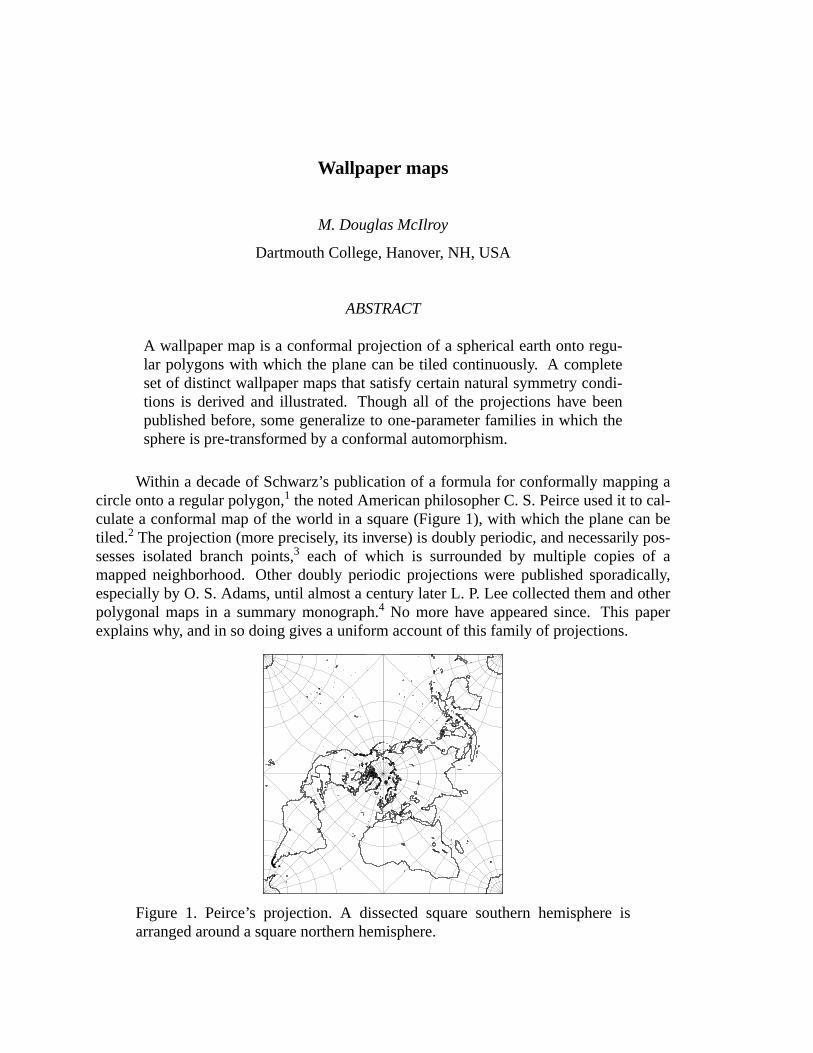
Within a decade of Schwarz’s publication of a formula for conformally mapping acircle onto a regular polygon,1 the noted American philosopher C. S. Peirce used it to cal-culate a conformal map of the world in a square (Figure 1), with which the plane can betiled.2 The projection (more precisely, its inverse) is doubly periodic, and necessarily pos-sesses isolated branch points,3 each of which is surrounded by multiple copies of amapped neighborhood. Other doubly periodic projections were published sporadically,especially by O. S. Adams, until almost a century later L. P. Lee collected them and otherpolygonal maps in a summary monograph.4 No more have appeared since. This paperexplains why, and in so doing gives a uniform account of this family of projections.

Figure 1. Peirce’s projection. A dissected square southern hemisphere isarranged around a square northern hemisphere.

-2-

Preliminaries

For our purposes, atiling is a covering of a surface by congruent, non-overlappingregular polygons, ortiles, fitted edge-to-edge and vertex-to-vertex. A tiling projection isa (one-to-many) conformal map from a tiling of the sphere to a tiling of the plane.Restricted to a single spherical tile and one of its planar image tiles, the map must

(a) beconformal and bijective throughout the interior,(b) continueacross each edge into an adjacent tile, conformally except at isolated

singularities,(c) preserve the symmetry group of each spherical tile, and(d) be the same in all tiles.

To state requirement (c) more precisely, let G andG′ be the (dihedral) symmetry groupsof a spherical polygon,X, and one of its planar images,X′, respectively; and letf : X → X′ be the mapping function.Then for eachg∈G there must exist g′∈G′ suchthat for every point x∈X

f (g(x)) = g′( f (x)) (1)

Requirement (d) says that tile-to-tile symmetries on the sphere and the plane com-mute with mapping from sphere to plane.If f acts on spherical tilesX andY to produceimages in planar tilesX′ andY′ respectively, and g is a symmetry operation on the spherethat takes tileX to Y, then there exists a symmetry operation,g′ on the plane that takesX′ to Y′ such that (1) holds for all pointsx in X.

The p lines of reflective symmetry in a sphericalp-gon must map onto lines ofreflective symmetry in the plane.In particular a vertex or the midedge of an edge (here-after called simply amidedge) of a spherical tile must map to a vertex or midedge (notnecessarily respectively) in the plane.Also, if p > 1, the center of a spherical tile mustmap to the center of a planar tile.

Call the vertices and midedges collectively fixable pointsand number the fixablepoints of a sphericalp-gon 0,1,. . . , 2p − 1 in order around the boundary, so that verticeshave even numbers and midedges odd. The fixable points of the correspondingp′-gonimage may be numbered similarly, with directions of increase being consistent under themap. Afixable point numberedx on a spherical tile maps to a fixable point numbered(kx + c) mod p′ on the planar image, where integerc represents a rotation andk = p′/p isa positive integer (Theorem 1 below). If k is even, both kinds of fixable point map to justone kind—vertex or midedge according asc is even or odd respectively. If k is odd, thekinds of fixable points are preserved whenc is even and exchanged whenc is odd. Forcontinuity (condition (b)), the parity ofc must be the same in every tile.

These observations are summarized in a table, in which V and M denote verticesand midedges; V,M → x, y means vertices map into fixable points of kindx and midedgesmap into kindy.

c ev en c oddk ev en V,M → V,V V,M → M,Mk odd V,M → V,M V,M → M,V

A tiling is completely characterized by its Schlafli symbol, {p, q}, which meanseach tile hasp edges (or vertices) and each vertex is surrounded byq tiles.5

-3-

Planar tilings comprise {3,6}, {4,4} and {6,3} (triangles, squares and hexagons).

Spherical tilings comprise {3,3}, {3,4}, {3,5}, {4,3} and {5,3} (corresponding tothe regular solids: tetrahedron, octahedron, icosahedron, cube and dodecahedron) plus theinfinite classes {2,n} ( gores) and {n,2} (hemispheres regarded as spherical polygonswith n 180° angles), wheren is a positive integer.6

In the degenerate case {2,1}, the sphere is cut by a slit that defines two coincidentedges. Theslit can be a great-circle arc of any positive length less than a circumference.We take apole-to-pole slit (making one 360° gore) as a canonical representative of thisuncountable subclass.Tiling projections based on {2,1} and its dual {1,2} will be dis-cussed under the heading ‘‘Conformal automorphisms of the sphere’’.

Characterization of tiling projections

Theorem 1. In a tiling projection from spherical tiling {p, q} to planar tiling{p′, q′}(i) p is a divisor of p′,(ii) if any spherical vertex maps onto a planar vertex, q is a divisor of q′,(iii) if any spherical vertex maps onto a planar midedge, qis 1 or 2, and(iv) if any spherical edge point maps onto a planar vertex, q′ is even.

Proof of (i). The symmetry group of a regular n-gon is the dihedral group of order2n, comprisingn rotations (including the identity) andn reflections. Property(i) followsfrom the facts that the order-2p group of a spherical tile is isomorphic to a subgroup ofthe order-2p′ group of its planar image, and the order of a subgroup is a divisor of theorder of a group.

The following lemma underlies the proofs of (ii)-(iv).

Lemma 1. If tile boundaries partition an arbitrarily small neighborhood of pointPon the sphere, with planar image P′, then a neighborhood ofP′ contains kimages ofeach set in the partition, where k is a positive integer.

Proof of Lemma 1.Let point x′ in the plane trace a simple circuit aroundP′ smallenough to exclude vertices distinct fromP′. For continuity, its preimagex must trace aclosed (not necessarily simple) circuitC that winds aroundP, traversing a sphericalpreimage tile for each traverse of one planar tile.For C to close,C must traverse everytile incident onP the same number of times.

Proof of (ii) and (iii). WhenP andP′ are vertices, the multiplicity in Lemma 1 isq′/q. whence property (ii). Property (iii) follows similarly from the fact that exactly 2planar tiles touch a midedge, soq must be a divisor of 2.

Proof of (iv). The edge partitions a small neighborhood of the spherical edge pointinto two parts. Thus,by Lemma 1,q′ must be a multiple of 2.

Corollary 1. In a tiling projection, the number, p, of vertices in a spherical tile isat most 4.

Proof. In a planar tiling, the number of vertices per tile is at most 6. Hence by The-orem 1, property (i), the numberp of vertices in a spherical tile is at most 6.For p = 6,the only admissible Schlafli symbols—{6,2} for the sphere and {6,3} for the plane—areruled out by property (ii), unless all 6 spherical vertices map to planar midedges. In that

-4-

case spherical midedges map to planar vertices, so by property (iv) q′ must be even (not3). Hencep < 6.

A spherical tiling withp = 5 is ruled out by the lack of planar tilings in whichp′ isa multiple of 5.

The remaining potential pairings of spherical and planar tilings are listed in Table1. Several of the projections lack standard names; I have taken the liberty of assigningshort nicknames to all of them*.Some tiling projections can be understood in multipleways. For example, Peirce’s projection (Figure 1) can be described as a map to squares{4,4} from 2 gores (2-vertex hemispheres) {2,2}, from 4 gores {2,4}, from 4-vertexhemispheres {4,2}, or from 1-vertex hemispheres {1,2} in two ways.

Table 1. Potential and actual tiling projections. Actual projections are calledby nickname and further described in Table 2. Roman numerals designatecases in Theorem 1 that prove impossibility. The starred entries generalize tofive distinct one-parameter families of projections.

Spherical Planartiling Planartilingtiling V →V V →M

{3,6} {4,4} {3,6} {4,4}M →M M →V M →V M →M

{1,2} Hex* Peirce* Hex* Peirce*{2,1} i Square* i Adams*{2,2} i Peirce i Peirce{2,3} i ii i ii{2,4} i Peirce i iii{2,6} i ii i ii{3,2} Hex i i ii i{3,3} Tetra i iii i{3,4} ii i i i i{4,2} i Peirce i Peirce{4,3} i ii i ii

Implementation

The first step in every construction is a standard conformal projection from sphereto plane. For all projections except Tetra, the second step is defined in terms of a stan-dard Schwarz transform, which maps the unit disc in thez-plane onto a regular n-gon inthew-plane:

w =z

0∫ (1 − zn)−2/ndz (2)

The z plane is cut from |z| = 1 to infinity along rays from the origin throughnth roots ofunity. Shifting the lower limit of the integral toz = 1, we obtain the alternate formula

* Peirce and Tetra were originally called ‘‘quincuncial’’ and ‘‘tetrahedric’’.

-5-

Table 2. Characteristics and origins of projections.Branch-point entriesb(e)give the number, b, of branch points of exponente on the boundary of eachplanar tile. The measure of angles at branch points in the plane ise times themeasure of corresponding angles on the sphere.

Nickname Figure;Table Tiles Branch Author, DateSpherical Planar Points

Peirce 1,2, 11; 3(a) hemisphere square 4(12) Peirce, 18792

Hex 12; 3(b) hemisphere triangle 3(13) Adams, 19257

Square 13;3(d), 4(b) 360° gore square 2(14), 2(12) Adams, 19298

Adams 14;4(c) 360°gore square 6(12) Adams, 19369

Tetra 15;3(c) tetrahedral triangle 3(12) Lee, 196510

triangle

w = wn +z

1∫ (1 − z)−2/n fn(z)dz (3)

where

wn

fn(z)

=

=

=

1

0∫ (1 − zn)−2/ndz

1

nΒ(1 /n, 1 − 2/n) =

Γ(1 /n)Γ(1 − 2/n)

n Γ(1 − 1/n)

1 − zn

1 − z

−2/n

Β and Γ are standard beta and gamma functions11 and fn(z) is analytic and nonzero atz = 1. From(3) we see that the transform multiplies, by a factor of (1− 2/n), the measureof angles between lines that meet atz = 1. In particular, the image of a smooth curve thatpasses throughz = 1 turns abruptly atw = wn making an angle of measure (1− 2/n)π .

Tetra involves a slight variant of the preceding scheme. In Table 3(c), the rhombusABCEhas anglesπ /3 and 2π /3 in the z-plane and angles twice as large on the sphere andon its stereographic image in thew-plane. Bysymmetry, the short diagonal on the sphere(arc AC in stereographic projection) maps to the short diagonal in thez-plane. The expo-nent−1/2 in the integrand realizes the halving of angles.

For some wallpaper maps, the Schwarz transform is applied, as shown in Table 3,to a conformal image of the sphere stereographically projected onto the closed complexplane. For others it is applied, as shown in Table 4, to an image projected onto the unitdisc by the Lagrange projection.

As inverses of doubly periodic functions, the wallpaper projections may beexpressed in terms of standard elliptic integrals.12 I hav e found, though, that workingdirectly from Schwarz integrals is computationally simpler than sophisticated elliptic-integral algorithms, and just as efficient for our purpose.

Expanding the integrand in (2) by the binomial theorem yields a power series rep-resentation of the transform, with radius of convergence 1.

-6-

w = z∞

k=0Σ

−2/n

k

(−1)k

k + 1znk (4)

To evaluate the transform near the singularity atz = 1, change variables in (3) to place thesingularity aty = 0.

w =

=

=

wn − ∫1−z

0(1 − (1 − y)n)−2/ndy

wn − ∫1−z

0

n

k=1Σ

n

k

(−1)k−1yk

−2/n

dy

wn − (1 − z)1−2/nFn(1 − z)

(5)

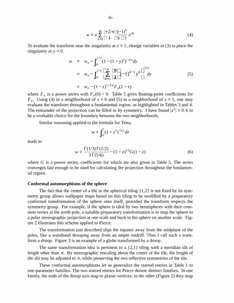
whereFn is a power series withFn(0) > 0. Table 5 gives floating-point coefficients forFn. Using (4) in a neighborhood ofz = 0 and (5) in a neighborhood ofz = 1, one mayevaluate the transform throughout a fundamental region, as highlighted in Tables 3 and 4.The remainder of the projection can be filled in by symmetry. I have found |z2| = 0. 6 tobe a workable choice for the boundary between the two neighborhoods.

Similar reasoning applied to the formula for Tetra,

w = ∫z

0(1 − z3)−1/2dz

leads to

w =Γ(1 / 3)Γ(1 / 2)

3Γ(5 / 6)− (1 − z)1/2G(1 − z) (6)

whereG is a power series, coefficients for which are also given in Table 5. The seriesconverges fast enough to be used for calculating the projection throughout the fundamen-tal region.

Conformal automorphisms of the sphere

The fact that the center of a tile in the spherical tiling {1,2} is not fixed by its sym-metry group allows wallpaper maps based on this tiling to be modified by a preparatoryconformal transformation of the sphere onto itself, provided the transform respects thesymmetry group.For example, if the sphere is tiled by two hemispheres with their com-mon vertex at the north pole, a suitable preparatory transformation is to map the sphere toa polar stereographic projection at one scale and back to the sphere on another scale.Fig-ure 2 illustrates this scheme applied to Pierce.

The transformation just described slips the equator away from the midplane of thepoles, like a waistband drooping away from an ample midriff. Thus I call such a trans-form adroop. Figure 3 is an example of a globe transformed by a droop.

The same transformation idea is pertinent to a {2,1} tiling with a meridian slit oflength other thanπ . By stereographic rescaling about the center of the tile, the length ofthe slit may be adjusted toπ , while preserving the two reflective symmetries of the tile.

These conformal automorphisms let us generalize the starred entries in Table 1 toone-parameter families. The two starred entries for Peirce denote distinct families. Inonefamily, the ends of the droop axis map to planar vertices; in the other (Figure 2) they map

-7-

Figure 2. An aspect of the Peirce projection devised independently byGuyou.13 At the top is a Peirce projection of two hemispheres. Atthe bot-tom, the hemispheres are regarded as {1,2} polygons with a lone vertex atthe north pole. A droop shifts parallel 15°S to the normal position of theequator, emphasizing Antarctica and the Southern Ocean at the expense ofthe Arctic Ocean and northern Eurasia.The vertex of each hemisphere ismapped to the midedge of the edge of a square.

to midedges. The two starred entries for Hex, however, yield only one family. In eachcase one end of the droop axis passes through a vertex, the other through a midedge.Thetwo cases differ only in regard to which end the droop is measured from.Thus the sixstarred entries give rise to only five distinct parameterized families.

The choice of parameter is quite like the choice of standard parallels in more famil-iar projections such as the Albers or Bonne projections. In fact a convenient way to spec-ify a polar droop is to name the parallel that becomes equidistant from the poles.

We now show that these generalizations exhaust the possibilities for wallpapermaps subject to the given symmetry conditions. The remainder of this section establishes

Theorem 2. The set of tiling projections comprises exactly the projections identifiedin Table 2. All but Tetra generalize to single-parameter families; Peirce generalizes intwo distinct ways.

In the following discussion, the terms ‘‘meridian’’, ‘ ‘parallel’’, ‘ ‘pole’’ and ‘‘equa-tor’’ generally refer to a mapped image of a standard spherical reticule, just as they do indiscussions of a flat map, although here the image happens to lie on a sphere.Several

-8-

properties of the standard reticule need not be preserved.

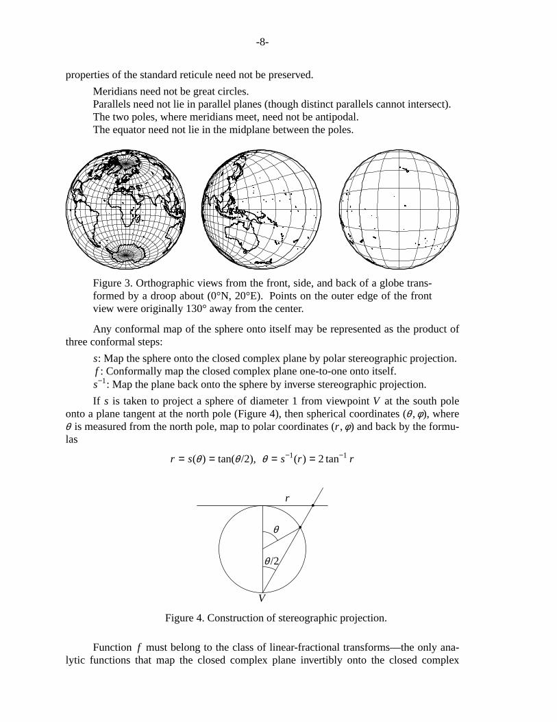
Meridians need not be great circles.Parallels need not lie in parallel planes (though distinct parallels cannot intersect).The two poles, where meridians meet, need not be antipodal.The equator need not lie in the midplane between the poles.

Figure 3. Orthographic views from the front, side, and back of a globe trans-formed by a droop about (0°N, 20°E).Points on the outer edge of the frontview were originally 130° away from the center.

Any conformal map of the sphere onto itself may be represented as the product ofthree conformal steps:

s: Map the sphere onto the closed complex plane by polar stereographic projection.f : Conformally map the closed complex plane one-to-one onto itself.s−1: Map the plane back onto the sphere by inverse stereographic projection.

If s is taken to project a sphere of diameter 1 from viewpoint V at the south poleonto a plane tangent at the north pole (Figure 4), then spherical coordinates (θ ,φ ), whereθ is measured from the north pole, map to polar coordinates (r ,φ ) and back by the formu-las

r = s(θ ) = tan(θ /2), θ = s−1(r ) = 2 tan−1 r

V

r

θ

θ /2

Figure 4. Construction of stereographic projection.

Function f must belong to the class of linear-fractional transforms—the only ana-lytic functions that map the closed complex plane invertibly onto the closed complex

-9-

plane.14

f (z) =az+ b

cz+ d, ad − bc ≠ 0

The four coefficients may be scaled arbitrarily (e.g. to makef = xn(1 + O(x)), n∈{ − 1, 0, 1} near x = 0). Hencethree parameters suffice to identifyany member of the class, from which fact follows

Corollary 2. A conformal automorphism of the sphere is determined by its behaviorat three points.

Besides preserving angles, all three steps map circles onto circles.14 (On the com-plex plane, straight lines count as circles of infinite radius.) Thus meridians and parallelsappear on the plane as two orthogonal systems of coaxal circles,15 illustrated in Figure 5.The meridians, which pass through the images of the north and south poles, form a coaxalsystem of ‘‘intersecting type’’. When the distance between poles is finite, the centers ofmeridians must lie on the perpendicular bisector of the segment determined by the poles.As on the sphere, parallels are trajectories orthogonal to the meridians and form a coaxalsystem of ‘‘nonintersecting type’’. Eachparallel is disjoint from the others and separatesthe two poles. When the distance between poles is finite, the centers of the parallels fallon the line determined by the poles. When one pole lies at infinity, meridians becomestraight lines radiating from the other pole and parallels become concentric circles.

(0,q)

(p, 0)(−k, 0)

Figure 5. Representative members of two orthogonal systems of coaxal cir-cles. Meridiansare centered on they axis and parallels on thex axis. Polesare at (± k, 0). Meridiansintersect parallels at right angles.Thick circles area typical parallel centered at (p, 0) with squared radiusp2 − k2, a typicalmeridian centered at (0,q) with squared radiusq2 + k2, and the smallestmeridian circle (radiusk).

-10-

If s is a polar stereographic projection, andf is a dilation about the pole by a factorof m, so that the transform is a droop, the inverse stereographic projection maps parallelθto θ ′ according to

θ ′/2 = tan−1 mr = tan−1(m tanθ /2)

When m ≠ 1, the projected parallels cluster towards one pole.The inverse of a droopwith dilation factorm is a droop about the same center with dilation factor 1/m, or equiv-alently a droop about an antipodal center with dilation factorm.

The conformal sphere-to-sphere transformations form an automorphism group thatacts on what I calldroopy spheres. In particular the group includes a transformation fromany droopy sphere onto astandard sphere, where the equator lies in the midplanebetween antipodal poles.

Lemma 2. A droopy sphere can be transformed to a standard sphere by a singledroop about an appropriate axis.

Proof of Lemma 2.If the poles of the droopy sphere are antipodal, pick any pointE on the equator. There exists a droop about a pole of a standard sphere that will makethe equator pass throughE while preserving the poles.With the behavior of three pointsknown, the transform is completely specified. Its inverse is the required transform.

Although we have described a droop as involving a dilation of the projection planeby some factorm, we can equally well view that as a dilation of the sphere by a factor of1/m. We shall do so for the rest of this section.

If the poles are not antipodal, consider first how to back-project arbitrary orthogo-nal systems of coaxal circles with two finite poles,N andS, and a distinguished equatoronto a standard sphere.Let E be the intersection of the equator and segmentNS. Figure6 shows a cross-section of a back-projection onto a standard sphere tangent toNS. Thecaption explains how to determine the point of tangency, orientation, and size of thesphere.

Figure 7 shows how to arrange for three points on a droopy sphere with pole-to-equator angles ofα and β to project to exactly the same three points as do the corre-sponding points on a standard sphere. The caption explains that, by rotating and dilatingthe two spheres appropriately,* their tangent points can be made to coincide.Therequired transformation is a droop about that point.

To complete the proof of Theorem 2, we note that a nontrivial droop preservesreflective symmetry only about planes through the axis of the droop.Hence, the axis of adroop applied to a {1,2} tiling of the sphere must pass through the single vertex throughwhich pass the plane of symmetry for each hemispheric tile and the plane of tile-to-tilesymmetry. Similarly, the axis of a droop applied to a {2,1} tiling must pass through thecenter of the single gore, where the gore’s two planes of symmetry meet. As these are theonly applicable droops, and the set of droops comprise all the nontrivial conformal auto-morphisms of the sphere, we have now characterized all admissible generalizations of thebasic tiling projections.

* Dilation and rotation parameters are calculated in Appendix 1.

-11-

N SEp

V1

Figure 6. Back projection onto a standard sphere from an arbitrary coaxalsystem in planep with polesN andS. A standard sphere, with tick marks atthe poles and equator, is placed with a meridian tangent to the unique straightmeridian in p. In p, the equator meets the straight meridian atE. Thedashed circles are the loci of viewpoints from whichNE and ES subtendπ /4; V1 is the unique viewpoint that achieves both.

Relaxed requirements

If the rather stringent conditions laid out among ‘‘Preliminaries’’ are relaxed, morewallpaper maps become possible. Some examples:

1. If the projection is not required to be the same in all tiles, then the composition ofany droop with any projection in Table 2 becomes admissible.

2. If a tile’s symmetry group is not required to be preserved, the Cox projection16

joins the menagerie.Cox maps a {2,1} 360°-gore tiling of the sphere onto an equi-lateral triangle (Table 6 and Figure 16), preserving only one of the gore’s tworeflective symmetries.*

3. If, further, tiles are not required to be regular polygons, then Peirce can bedescribed in yet another way: a map from a {3,4} octahedral spherical tiling withangles (π2,

π2,

π2 ) to a planar tiling by triangles with angles (π

2,π4,

π4 ).

Enough. Systematic investigation of plausible generalizations is a topic for another time.

Acknowledgments

Long before I knew most of the literature cited in this paper, I showed Peirce to thelate Robert Morris. He asked, ‘‘Can you do the same thing with triangles?’’ That preg-nant question spurred a lasting interest in wallpaper maps.

I am grateful to Daan Strebe for pointing out references in earth-sciences literature.

* A dams suggested the projection in 1925, but chose not to compute it.7 ,

-12-

N SEp

d1

T1T2

d2

V1

V2

α /2β /2

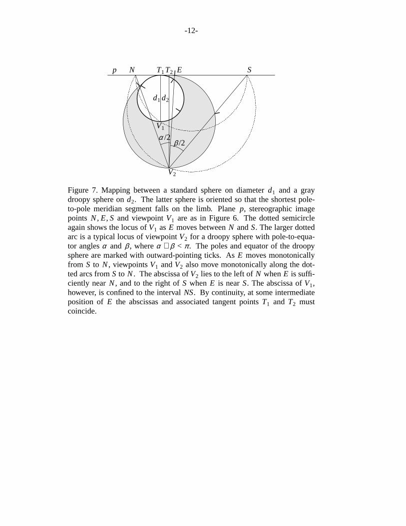
Figure 7. Mapping between a standard sphere on diameterd1 and a graydroopy sphere ond2. The latter sphere is oriented so that the shortest pole-to-pole meridian segment falls on the limb. Plane p, stereographic imagepoints N, E, S and viewpoint V1 are as in Figure 6. The dotted semicircleagain shows the locus ofV1 asE moves betweenN andS. The larger dottedarc is a typical locus of viewpoint V2 for a droopy sphere with pole-to-equa-tor anglesα and β , whereα + β < π . The poles and equator of the droopysphere are marked with outward-pointing ticks.As E moves monotonicallyfrom S to N, viewpointsV1 andV2 also move monotonically along the dot-ted arcs fromS to N. The abscissa ofV2 lies to the left ofN whenE is suffi-ciently nearN, and to the right ofS when E is nearS. The abscissa ofV1,however, is confined to the interval NS. By continuity, at some intermediateposition of E the abscissas and associated tangent pointsT1 and T2 mustcoincide.

-13-

Table 3. Construction of projections. Each left panel shows a stereographic projection inthe complex z-plane. In(a), (b) and (c) the north pole is atz = 0 and argz measures lon-gitude. In(d) the north pole is at atz = −1 and the south is atz = 1. Thez-plane is cutfor a Schwarz transformation and scaled so cuts end on the unit circle. Similarly namedlabels (e.g. B, B′) identify distinct approaches to the point at infinity, whose imagesapproach a single point (B) in the w-plane. Theequator is drawn with fine dashes, butonly when it is circular or (piecewise) straight.Representative vertices in thew-plane arelabeled by the ratioq/q′, with 1/1 for a point interior to a hemispheric tile. Branch-pointexponents in the Schwarz integrals areq/q′ − 1. A shaded triangle designates a funda-mental region from which the projection can be extended to the rest of thew-plane imageby symmetry. (Computational formulas (4), (5) and (6) apply directly to both the funda-mental region and its reflection in the real axis.)

(a) Peirce

H ′A

B

B′

C

D

D′E

F

F ′

G

H

A 2/4

B 1/1CD

E

F G H

w = ∫z

0(1 − z4)−1/2dzz

→

-14-

Table 3 (continued)

(b) Hex

F ′A

B

B′

C

D

D′

E

F

A 2/6

B 1/1C

D

E F

w = ∫z

0(1 − z3)−2/3dzz

→

(c) Tetra

F ′AB

B′

C

D

D′

E

F

A 3/6

B 3/6

C

D

E

F

w = ∫z

0(1 − z3)−1/2dz

z

→

Spherical tileACE has 120° anglesand vertices at latitude arcsin1/3.

(d) Square (alternate construction)

D′′A

BB′′C

D

B′

D′

A 1/4

B 2/4

C

D

w = ∫z

0(1 − z2)−3/4dzz

→

Fundamental region has 2 branch points;see Table 4(b) for simpler construction

-15-

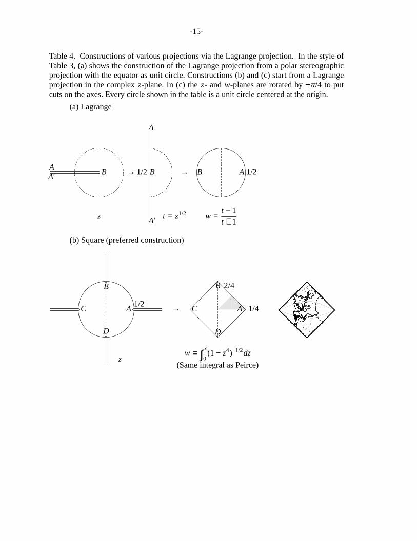
Table 4. Constructions of various projections via the Lagrange projection. In the style ofTable 3, (a) shows the construction of the Lagrange projection from a polar stereographicprojection with the equator as unit circle. Constructions (b) and (c) start from a Lagrangeprojection in the complex z-plane. In (c) thez- and w-planes are rotated by−π /4 to putcuts on the axes. Every circle shown in the table is a unit circle centered at the origin.

(a) Lagrange

AB

A′

A

1/2 B

A′

A 1/2B

z t = z1/2 w =t − 1

t + 1

→ →

(b) Square (preferred construction)

A

B

C

D

1/2A 1/4

B 2/4

C

D

zw = ∫

z

0(1 − z4)−1/2dz

(Same integral as Peirce)

→

-16-

Table 4 (continued)

(c) Adams

A1/2

D2/2

F

B

C

E

t = e−iπ /4z

A1/2

DB 2/4

C

E

F

e−iπ /4w = ∫t

0(1 − t4)−1/2dt

(Same integral as Peirce)

→

Table 5. Coefficients for power series in equations (5) and (6).A power-series package17

was used to calculate (rational) coefficients forn2/nFn and 31/2G, from which floating-point coefficients ofkth powers inFn andG were derived. w(1) is the value ofw at z = 1in (5) or (6).

k F3 F4 G

0 1.44224957030741 1.0 1.154700538379251 0.240374928384568 0.25 0.1924500897298752 0.0686785509670194 0.06875 0.04811252243246873 0.0178055502507087 0.0078125 0.0103098262355294 0.00228276285265497 -7.64973958333333×10−3 3.34114739114366×10−4

5 -1.48379585422573×10−3 -0.0069580078125 -1.50351632601465×10−3

6 -1.64287728109203×10−3 -2.89330115685096×10−3 -1.23044177962310×10−3

7 -1.02583417082273×10−3 -2.0599365234375×10−5 -6.75190201960282×10−4

8 -4.83607537673571×10−4 9.95881417218377×10−4 -2.84084537293856×10−4

9 -1.67030822094781×10−4 8.64356756210327×10−4 -8.21205120500051×10−5

10 -2.45024395166263×10−5 3.85705381631851×10−4 -1.59257630018706×10−6

11 2.14092375450951×10−5 1.40434131026268×10−5 1.91691805888369×10−5

12 2.55897270486771×10−5 -1.34721419308335×10−4 1.73095888028726×10−5

13 1.73086854400834×10−5 -1.24614486897675×10−4 1.03865580818367×10−5

14 8.72756299984649×10−6 -5.74855643333586×10−5 4.70614523937179×10−6

15 3.18304486798473×10−6 -1.12228690340999×10−6 1.4413500104181×10−6

16 4.79323894565283×10−7 2.27285782088416×10−5 1.92757960170179×10−8

17 -4.58968389565456×10−7 2.12777819566412×10−5 -3.82869799649063×10−7

18 -5.62970586787826×10−7 9.99206810770337×10−6 -3.57526015225576×10−7

19 -3.92135372833465×10−7 1.83254758167307×10−7 -2.2175964844211×10−7

w(1) 1.76663875028545 1.31102877714606 1.40218210532545

-17-

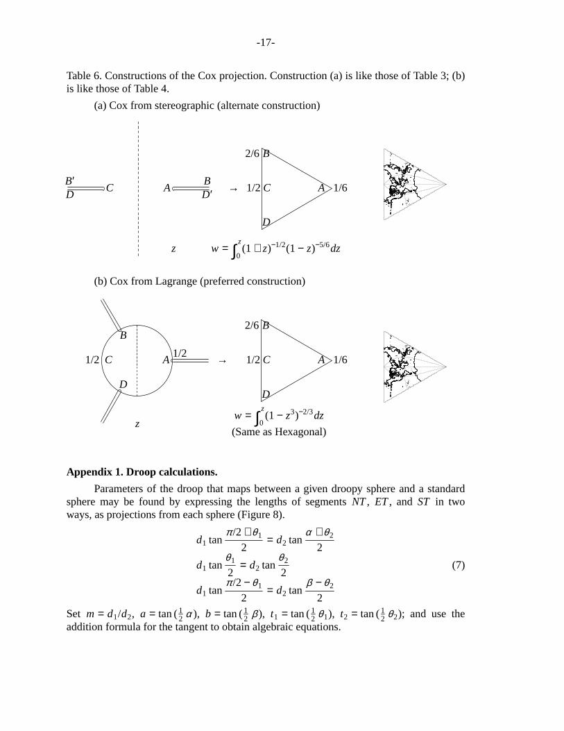
Table 6. Constructions of the Cox projection. Construction (a) is like those of Table 3; (b)is like those of Table 4.

(a) Cox from stereographic (alternate construction)

D′ABB′

CD

A 1/61/2C

2/6 B

D

w = ∫z

0(1 + z)−1/2(1 − z)−5/6dzz

→

(b) Cox from Lagrange (preferred construction)

A

B

D

1/2 C1/2

A 1/61/2C

2/6 B

D

zw = ∫

z

0(1 − z3)−2/3dz

(Same as Hexagonal)

→

Appendix 1. Droop calculations.

Parameters of the droop that maps between a given droopy sphere and a standardsphere may be found by expressing the lengths of segmentsNT, ET, and ST in twoways, as projections from each sphere (Figure 8).

d1 tanπ /2 + θ1

2= d2 tan

α + θ2

2

d1 tanθ1

2= d2 tan

θ2

2

d1 tanπ /2 − θ1

2= d2 tan

β − θ2

2

(7)

Set m = d1/d2, a = tan (12 α ), b = tan (12 β ), t1 = tan (12 θ1), t2 = tan (12 θ2); and use theaddition formula for the tangent to obtain algebraic equations.

-18-

m1 + t1

1 − t1=

a + t2

1 − at2mt1 = t2

m1 − t1

1 + t1=

b − t2

1 + bt2

(8)

The only real solutions of (8) (found by Maple*)18 entailed

m =2a2b2 + a2 + b2 ± (4a2b2(1 − ab)2 + (a2 − b2)2 )

12

2ab(a + b)(9)

To choose between the two roots, consider the caseα = β , or equivalently a = b. Then,Figure [1projaxis] becomes symmetric, withT midway between N and S, andθ1 = θ2 = 0. Hence,from Figure 9,m = d1/d2 = tan (12 α ) = a. Specialized toa = b, (9)becomes

m =1 + a2 ± ( (1 − a2)2 )

12

2a(10)

N S

d2

d1

Tθ2Eθ1

α /2β /2

Figure 8. A standard sphere and a droopy sphere with a common point oftangency, T. θ1 andθ2 are azimuths of the equator measured at the center ofthe spheres relative to the point of tangency.

Becauseα + β < π , the assumptionα = β impliesa = tan (12 α ) < tan (14 π ) = 1. Thusthepositive square root of (1− a2)2 is 1− a2. For (10) to evaluate tom = a, the± sign in (9)must be taken as−, provided the square root is understood to be positive.

To find t1, eliminate t2 from (8) by simple substitution; solve each of the remainingequations fort2

1; and equate the two results.

* The Maple version that I used could solve the system only aftert2 had been triviallyeliminated.

-19-

m − a − a(m2 − 1)t1

m(am− 1)=

m − b + b(m2 − 1)t1

m(bm− 1)

Whence

t1 =a − b

2amb− b − a

Further routine manipulation leads to the complete solution of (8).

d1

d2= m =

2a2b2 + a2 + b2 − √ D2ab(a + b)

tan (12 θ1) = t1 =2a2b2 − 2ab+ √ D

a2 − b2

tan (12 θ2) = t2 =2a2b2 − a2 − b2 + √ D

2ab(a − b)

(11)

where

D = 4a2b2(1 − ab)2 + (a2 − b2)2

a = tan(12 α )

b = tan(12 β )

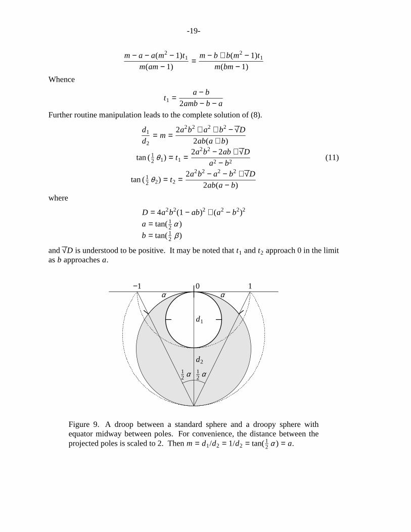
and√ D is understood to be positive. It may be noted thatt1 andt2 approach 0 in the limitasb approachesa.

−1 10

d1

d2

α α

12 α 1

2 α

Figure 9. A droop between a standard sphere and a droopy sphere withequator midway between poles.For convenience, the distance between theprojected poles is scaled to 2. Thenm = d1/d2 = 1/d2 = tan(12 α ) = a.

-20-

The shape of a droopy sphere

On a droopy sphere, meridians and parallels, being circles, lie in planes.Clearlythe planes of meridians meet in the line joining the two poles. Ingeneral, the planes ofparallels also meet in a common line, which must fall outside the sphere because parallelscan’t intersect (Figure 10).

Theorem 3. On a droopy sphere the planes of parallels concur in the line of inter-section of planes tangent to the sphere at the two poles, or are parallel when the poles areantipodal.

Proof. When the poles are antipodal, the droopy sphere can be transformed to astandard sphere by a polar droop. Hence the planes of parallels must be parallel.

Otherwise, as we have seen, every droopy sphere is the inverse stereographic imageof an orthogonal pair of systems of coaxal circles, with meridians meeting at two finitepoints. Parametric equations for such systems can be read off f rom Figure 5.

(x − p)2 + y2 = p2 − k2, parallels

x2 + (y − q)2 = q2 + k2, meridians

These equation simplify to

x2 + y2 − 2px + k2 = 0 (12)

x2 + y2 − 2qy − k2 = 0 (13)

Consider, without loss of generality, the inverse stereographic projection of systemsof coaxal circles in the planez = 1 (in Euclidean 3-space) onto a sphere of diameter 1tangent toz = 1 at (0,0,1) with an antipodal center of perspective at (0,0,0). Theequationof this sphere is

x2 + y2 + (z − 1/2)2 = (1 / 2)2

or

x2 + y2 + z2 − z = 0 (14)

To account for arbitrary positioning of the coaxal systems relative to the sphere,move the center of the coaxal systems to (a, b) by replacing x and y by (x − a) and(y − b) in (12) and (13).Circles of the systems are projected on sphere (14) by intersect-ing it with cones that have vertex (0,0,0) and coincide with the specified circles whenz = 1.

(x − az)2 + (y − bz)2 − 2pz(x − az) + (kz)2 = 0 (15)

(x − az)2 + (y − bz)2 − 2qz(y − bz) − (kz)2 = 0 (16)

To find the intersection for a parallel, first subtract (14) from (15).

−2axz+ a2z2 − 2byz+ b2z2 − 2pxz+ 2apz2 − z + z − (kz)2 = 0

Factor outz to get an equation for the plane of the parallel.

-21-

−2(a + p)x − 2by + (a2 + b2 + 2ap− 1 − k2)z + 1 = 0 (17)

The intersection of two such planes for infinitesimally different values ofp must satisfythe equation resulting from differentiating with respect top.

−2x + 2az = 0 (18)

Thus the line of intersection lies in the planex = az. Substitute the value of 2x from (18)into (17) to find the equation of another plane in which the the line of intersection lies.

−2by + (b2 − a2 − 1 − k2)z + 1 = 0 (19)

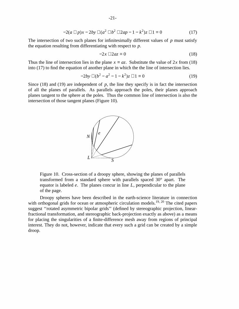
Since (18) and (19) are independent ofp, the line they specify is in fact the intersectionof all the planes of parallels.As parallels approach the poles, their planes approachplanes tangent to the sphere at the poles. Thus the common line of intersection is also theintersection of those tangent planes (Figure 10).

L

eN

S

Figure 10. Cross-section of a droopy sphere, showing the planes of parallelstransformed from a standard sphere with parallels spaced 30° apart.Theequator is labelede. The planes concur in lineL, perpendicular to the planeof the page.

Droopy spheres have been described in the earth-science literature in connectionwith orthogonal grids for ocean or atmospheric circulation models.19, 20The cited paperssuggest ‘‘rotated asymmetric bipolar grids’’ (defined by stereographic projection, linear-fractional transformation, and stereographic back-projection exactly as above) as a meansfor placing the singularities of a finite-difference mesh away from regions of principalinterest. They do not, however, indicate that every such a grid can be created by a simpledroop.

-22-

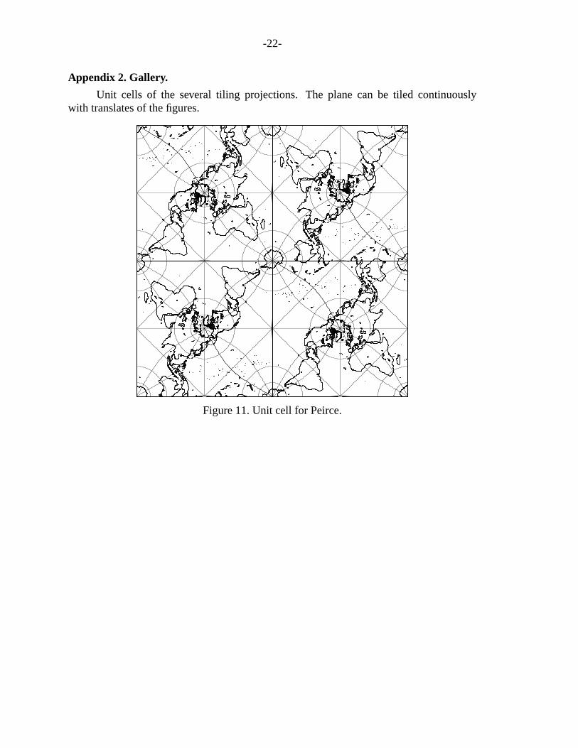
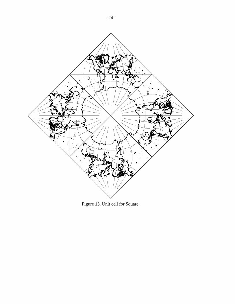
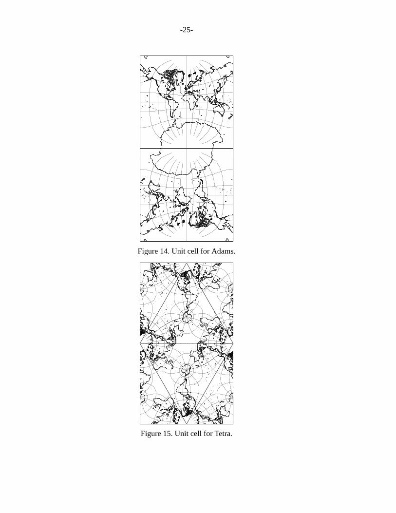
Appendix 2. Gallery.

Unit cells of the several tiling projections. The plane can be tiled continuouslywith translates of the figures.

Figure 11. Unit cell for Peirce.

-23-

Figure 12. Unit cell for Hex.

-24-

Figure 13. Unit cell for Square.

-25-

Figure 14. Unit cell for Adams.

Figure 15. Unit cell for Tetra.

-26-

Figure 16. Unit cell for Cox. Qualifies as a tiling projection only underrelaxed symmetry conditions.

-27-

References

1. H. A. Schwarz, “Uber einige Abbildungsaufgaben,”Journal fur die reine un ange-wandte Mathematik,schwarz70, pp. 105-120.

2. C.S. Peirce, “A quincuncial projection of the sphere,” American Journal of Mathe-matics,peirce2, pp. 394-396 and one unpaginated plate (1879).

3. E.T. Whittaker and G. N. Watson,A Course of Modern Analysis,whittaker, Cam-bridge (1927).

4. L. P. Lee, “Conformal Projections Based on Elliptic Functions,” CartographicaMonograph No. 16, University of Toronto Press (1976).

5. H. S. M. Coxeter,Regular Polytopes,coxeter, Dover (1973). Reprint of Macmillanedition of 1963.

6. H.We yl, Symmetry,weyl, Princeton University Press (1952).

7. O. A. Adams, “Elliptic Functions Applied to Conformal World Maps,” Specialpublication No. 112, U.S. Coast and Geodetic Survey (1925).

8. O.A. Adams, “Conformal Projection of the Sphere within a Square,” Special publi-cation No. 153, U.S. Coast and Geodetic Survey (1929).

9. O. A. Adams, “Conformal map of the world in a square,” Bulletin Geod esique,adams, pp. 461-473 (1936).

10. L. P. Lee, “Some conformal projections based on elliptic functions,” GeographicalReview, lee55, pp. 563-580 (1965).

11. M.Abramowitz and I. A. Stegun, “Handbook of Mathematical Functions with For-mulas, Graphs, and Mathematical Tables,” A pplied Mathematics Series no. 55,National Bureau of Standards (1965).

12. J. P. Snyder and P. M. Voxland, “An Album of Map Projections,” ProfessionalPaper 1453, U.S. Geological Survey (1989). Elliptic integrals for square tilings.

13. E.Guyou, “Sur un nouveau systeme de projection de la sphere,” Comptes Rendusde l’Acad*’emie des Sciences,guyou102, pp. 308-10 (1886).

14. L. Bieberbach,Conformal Mapping, bieberbach, Chelsea (1953). Translated by F.Steinhardt.

15. D.Pedoe,Geometry: A Comprehensive Course,Dover (1988).

16. J. F. Cox, “Representation de la surface entiere de la terre dans une triangleequilat eral,” Bulletin de la Classe des Sciences, Academie Royale de Belgique, cox5e, 21, pp. 66-71 (1935).

17. M. D. McIlroy, “Power Series, Power Serious,” Journal of Functional Program-ming,mcilroy 9, pp. 325-337 (1999).

18. Waterloo Maple, Inc.,Maple User Manual,Waterloo, ON, Canada.

19. R.J. Murray, “Explicit generation of orthogonal grids for ocean models,” Journalof Computational Physics,murray126, pp. 251-273 (1996).

20. M. Bentsen, G. Evensen, H. Drange, and A. D. Jenkins, “Coordinate transforma-tion on a sphere using conformal mapping,” Monthly Weather Review, bentsen127,pp. 2733-2740, American Meteorological Society (1999).

-28-