NBER WORKING PAPER SERIES

SEASONAL CREDIT CONSTRAINTS AND AGRICULTURAL LABOR SUPPLY:EVIDENCE FROM ZAMBIA

Günther FinkB. Kelsey JackFelix Masiye

Working Paper 20218http://www.nber.org/papers/w20218

NATIONAL BUREAU OF ECONOMIC RESEARCH1050 Massachusetts Avenue

Cambridge, MA 02138June 2014

We thank Seema Jayachandran and audiences at University of Cape Town SALDRU, the Universityof Washington, the University ofWisconsin-Milwaukee, the University of Zambia, the UC Berkeleydevelopment lunch, the Harvard Development faculty retreat, the Gates Foundation, IGC Growth Weekand PacDev for comments and suggestions. We are grateful to the International Growth Centre andthe Agricultural Technology Adoption Initiative (JPAL/CEGA) for financial support and to Innovationsfor Poverty Action for logistical support. Austin Land and Chantelle Boudreaux provided excellentassistance with the field work and data, respectively. The views expressed herein are those of the authorsand do not necessarily reflect the views of the National Bureau of Economic Research.

NBER working papers are circulated for discussion and comment purposes. They have not been peer-reviewed or been subject to the review by the NBER Board of Directors that accompanies officialNBER publications.

© 2014 by Günther Fink, B. Kelsey Jack, and Felix Masiye. All rights reserved. Short sections of text,not to exceed two paragraphs, may be quoted without explicit permission provided that full credit,including © notice, is given to the source.

Seasonal Credit Constraints and Agricultural Labor Supply: Evidence from ZambiaGünther Fink, B. Kelsey Jack, and Felix MasiyeNBER Working Paper No. 20218June 2014JEL No. J22,O16,Q12

ABSTRACT

Small-scale farming remains the primary source of income for a majority of the population in developingcountries. While most farmers primarily work on their own fields, off-farm labor is common amongsmall-scale farmers. A growing literature suggests that off-farm labor is not the result of optimal laborallocation, but is instead driven by households’ inability to cover short-term consumption needs withsavings or credit. We conduct a field experiment in rural Zambia to investigate the relationship betweencredit availability and rural labor supply. We find that providing households with access to credit duringthe growing season substantially alters the allocation of household labor, with households in villagesrandomly selected for a loan program selling on average 25 percent less off-farm labor. We also findthat increased credit availability is associated with higher consumption and increases in local farmingwages. Our results suggest that a substantial fraction of rural labor supply is driven by short-termconstraints, and that access to credit markets may improve the efficiency of labor allocation overall.

Günther FinkHarvard School of Public HealthDepartment of Global Health and Population665 Huntington Ave.Boston, MA 02115gfink@hsph.harvard.edu

B. Kelsey JackDepartment of EconomicsTufts University314 Braker HallMedford, MA 02155and NBERkelsey.jack@tufts.edu

Felix Masiye Department of Economics University of Zambia Lusaka, Zambia fmasiye@yahoo.com

1 Introduction

In Zambia, like in much of Sub-Saharan Africa, agriculture employs the vast majority of therural population, with generally low levels of productivity and farming income.1 A lack ofirrigation infrastructure combined with a long dry season mean that harvest income arrivesonly once per year, and must cover household needs for the subsequent 10-12 months. Ifavailable resources are insufficient to cover consumption needs, households can either financeconsumption gaps through credit or engage in alternative consumption smoothing strategiesincluding off-farm labor.2 From a household production perspective, selling family laboroff-farm can be optimal as long as the marginal product of labor off-farm is higher than themarginal product of labor on the farm. However, a growing literature suggests that off-farmlabor reflects a coping strategy rather than income maximization (Kerr 2005; Bryceson 2006;Orr et al. 2009; Michaelowa et al. 2010; Cole and Hoon 2013). The logic of the underlyingargument is simple: since most small scale farmers have limited ownership of liquid assetsand virtually no access to short-term credit, the least costly (or only possible) way to financeshort-term consumption may be to generate wage income from local labor markets.

Conceptually, frictions in the credit market may thus lead to two inefficiencies in thefarm’s production schedule. First, the farm may alter the the total quantity of land used andcrop mix chosen to ensure that the available family labor, net of anticipated work requiredoff-farm, is sufficient to maximize yields. In most settings, the production plan chosen inthe constrained environment will not be the same as the optimal choice in an unconstrainedenvironment (Fafchamps 1993; Rosenzweig and Binswanger 1993), which may lower thefarm’s net income. Second, these extensive margin or ex ante inefficiencies can be furthercompounded by intensive margin inefficiencies if households experience unanticipated incomeor expenditure shocks during the farming season. To cover short-term consumption andliquidity needs, farming households may deviate from their original (adjusted) productionplan by reallocating labor to earn off-farm wages (Kochar 1995, 1999; Rose 2001; Ito andKurosaki 2009).3

1A recent study in the region of proposed research shows average gross production value of USD 500 fora family of six (Fink and Masiye 2012). Once capital input, land and labor costs are considered, net profitsfor many of these families may be negative.

2Most rural households own some assets such as livestock, agricultural livestock or cooking ware whichthey could theoretically liquidate; in practice, finding a buyer for such assets during the most constrainedperiods may be difficult, and the transaction cost of liquidating assets may be prohibitive.

3Common income shocks in the area are the loss of stored food reserves due to pests or theft; expenditureshocks include funerals, school uniforms and medical costs.

2

To investigate the relationship between credit availability and agricultural labor supply,we conducted a cluster-randomized experiment with small-scale farmers from selected villagesin rural Zambia. As shown by the descriptive plots in in Figures 1 and 2 food shortages andoff-farm labor (locally referred to as ganyu) are common in the study area, with pronouncedseasonal patterns.4 Zambia’s agricultural cycle is centered around the rainy season fromNovember to April. Harvest takes place in May and June, and generates income that mustcover all consumption and investment needs until the following year’s harvest. Householdreserves are diminished by the beginning of the rainy season (six months after harvest), andare most scarce from January to March before early crops become available for consumption.The January to March period is generally referred to as the “hungry season” by farmers, andis the period we directly targeted with the intervention. The intervention offered selectedsmall-scale farming households access to interest-free maize loans to be repaid in kind afterharvest, approximately 3 months after the last loan installment was received. The maximumloan size was 3 bags of ground maize, a quantity large enough to cover the consumption needsof an average household over a three-month period.5 Treatment intensity was varied at thevillage level, with a smaller fraction of households receiving loans in partial (as opposed tofull) treatment villages.

Both the demand for and the willingness to repay loans was high, with over 90 percenttake up among eligible households and close to 95 percent repayment. To assess the impact ofloans on local labor markets and labor allocation decisions, we develop a series of predictionsthrough a simple agricultural labor market model, and test them empirically using ourexperimental data. Consistent with the model, we find relatively large effects of the loanson off-farm labor supply. In villages where all farmers were eligible for the maize loan,the probability that a household reported off-farm labor over a two week period during thehungry season fell by around 25 percent (11.8 percentage points). In the same villages, thetotal number of days of ganyu reported fell by around one-third, with a corresponding (butstatistically imprecise) increase in the number of days worked on-farm. We also test whetherthe reduction in off-farm labor during the hungry season is offset by an increase in off-farm

4Seasonality in food consumption may reflect an optimal response to seasonal price variation. As shownin Appendix figure A.1, seasonal fluctuations in maize prices are less pronounced in Zambia than in othernearby countries (see, for example, Burke (2014)).

5Households could receive up to 75 kilograms (in 25 kg bags) of ground “breakfast meal” maize, whichthey had to repay with 150 kilograms harvested (ungrounded) maize. A 50 kilogram bag of unground maizeyields approximately 25 kilograms of ground maize; the market value of the ground maize received and theharvested maize paid back is very similar. Households in the program therefore receive a transfer equal tothe value of the interest on the loan. In Section 3, we calibrate the size of the transfer.

3

labor to generate resources to repay the loan. In the two months preceding loan repayment,reported off-farm casual labor was significantly lower in treated villages, and the overallprobability of doing any casual labor at any point during the entire agricultural season was9.1 percentage points lower in the fully treated villages than in the control villages.

Consistent with the observed reductions in farmers’ willingness (or need) to engage inoff-farm labor, we find sizable increases in average wages paid locally for off-farm labor. Infully treated villages, the average wage reported among (the smaller number of) workersengaging in ganyu increased by almost 50 percent immediately following the loan transfersand by 25 to 35 percent over the treatment period. The wage effects were smaller butremain positive in partial treatment villages, where only 50 percent of farmers were eligiblefor the loan program. We also find substantial declines in reported hunger in treated villages.Specifically, the intention-to-treat (ITT) estimates show that in villages where all householdswere eligible for the loan, the number of meals consumed by the respondent in the 24 hourspreceding the survey increased by 11 percent (0.2 more meals) and household members werealmost 50 percent (16.5 percentage points) less likely to miss meals due to food shortages inthe week before the survey.

For both the consumption and the labor allocation results, the observed effect sizesare smaller in partial treatment villages, with relatively large - but imprecisely estimated -spillovers for households whose neighbors receive loans. All of the data collected suggeststhat these spillovers are not the result of within community sharing or redistribution ofresources: we observe no effect of treatment on reported gifts, loans or transfers amongeligible or ineligible households. Given the large wage response, some positive spilloversthrough the labor market seem likely, since higher local wages allow ineligible householdsto meet their consumption needs with fewer hours of off-farm labor. The relatively smallsample size of the study does not allow us to precisely pin down the magnitude of the laborsupply elasticity. Larger studies in this area would help to isolate the channels underlyingthe observed spillover and general equilibrium effects.

The results presented in this paper are linked to a large literature in development eco-nomics documenting the often complex and seasonal nature of rural labor supply (for areview, see Rosenzweig 1988). A number of previous studies have investigated households’use of off-farm labor to smooth consumption in response to, or anticipation of, productivityshocks (Kochar 1995, 1999; Rose 2001; Ito and Kurosaki 2009), suggesting that productivityshocks may alter labor supply and affect rural wages. Consistent with the findings in thispaper, Jayachandran (2006) shows that incomplete credit markets lower the elasticity of

4

labor supply, further increasing wage volatility. Mobarak and Rosenzweig (2014) show thatwage volatility is reduced and sizable welfare improvements are possible when workers canbe insured against aggregate shocks. More recently, a growing number of field experimentsexamine labor supply determinants in developing country settings, some of which shed lighton questions of seasonality and consumption constraints. For example, Goldberg (2013) findsvery low labor supply elasticities following the harvest period in Malawi. Also in Malawi,Guiteras and Jack (2014) examine labor supply during the hungry season and after harvestand note the seasonal coincidence of high labor demand and liquidity constraints.6

The results in this paper are also linked to a larger literature on consumption smooth-ing. In the face of missing credit markets, households may resort to a range of consumptionsmoothing strategies, ranging from livestock and asset sales to migration (for summariesof the literature, see Morduch (1995) and Besley (1995)). The substantial increase in con-sumption that we observe among treated households during the hungry season suggests thatfarming households in the study adjust to resource scarcity not only through off-farm la-bor, but also by reducing consumption during the growing season, where caloric needs arelikely highest. These reductions in calorie intake during the peak labor season are also con-sistent with a related nutrition-focused literature which suggests that farmers’ constrainednutritional intake leads to suboptimal production (Pitt and Rosenzweig 1986; Strauss 1986;Behrman et al. 1997), an idea also supported by recent evidence from India (Schofield 2013).

The general relationship between income seasonality and consumption smoothing is notwell established in the literature. While some studies suggest that precautionary savings aresufficient to smooth consumption even if income is highly seasonal (Paxson 1993; Chaudhuriand Paxson 2002), others have highlighted the pronounced consumption differences betweenlean or hungry season (Dercon and Krishnan 2000; Khandker 2012), consistent with thepatterns shown in Figure 2.

Few studies have examined the impact of explicitly seasonal transfer or loan programs.Burke (2014) offered farmers in Kenya a loan product that allowed them to exploit seasonalvariation in maize prices and finds significant effects on total maize revenues and householdexpenditures. Bryan, Chowdhury and Mobarak (2013) provide credit and grants for shortrun seasonal labor migration in Bangladesh and argue that credit market failures and highlyuncertain returns likely keep long-distance labor supply below welfare-maximizing levels.

6Inefficient labor supply does not, however, imply credit or liquidity constraints. In a nonagriculturalsetting, Dupas and Robinson (2014) rule out consumption constraints as a driver of decisions in their studyof reference dependent labor supply among bicycle taxis in Kenya.

5

Most similar to our study, Basu and Wong (2012) study a seasonal food credit programin Indonesia and find that food loans increase consumption during the lean season, but donot analyze labor supply impacts. Our findings contribute to that literature by providingthe first direct evidence that seasonal food shortages drive off-farm labor supply and localwages. We also show that relaxing credit constraints leads to an adjustment of householdlabor supply and an equilibrium increase in local wages. Both the labor supply and the wageresults are the product of multiple different margins adjusting as credit markets are relaxed,including better nutrition, a lower number of credit-constrained households and differentialselection into the off-farm labor market. In terms of final labor allocation, the relaxationof credit constraints reallocated labor from relatively better-off farms able to hire ganyu tosmaller farms generally dependent on doing ganyu as a coping mechanism.

The paper proceeds as follows. In the next section, we present a simple model of agri-cultural labor decisions in the presence of credit constraints. Section 3 describes the studycontext, experimental design and implementation. Section 4 sets up the identification strat-egy. Section 5 presents the results, and Section 6 concludes.

2 Conceptual framework

Consider a simple two-period model of agricultural production, where rational farming house-holds maximize their utility over consumption and leisure. In the first period (the growingseason), households make their labor and consumption decision. In the second period (theharvesting season), households collect the harvest outcomes and get utility from consumingthe harvest outcomes. Land endowments are fixed. There are two types of farms: thosewith relatively large capital endowments that are net buyers of labor, and small-scale farms,which divide their labor between their own farm and off-farm work at a locally determinedwage rate w. For ease of exposition, we refer to the former as large and the latter small,though land size need not differ between the farm types. Large farms, indexed by b, choosetheir labor inputs optimally to maximize profits such that

Y�

b (l∗b ) = w (1)

where Y �b (l) is the marginal product of labor on the large farm, with Y

�(l) > 0 and Y

��(l) < 0,

and w is the local wage rate. Small-scale farmers have their own land, and maximize theirutility u(.), which is an increasing and concave function of consumption c and leisure time

6

f. We assume that small farmers have a fixed time endowment T , which they can allocateto selling labor off-farm to the large farms (lo), to work on their own farm (ls), or for leisuref , so that the time budget constraint is given by

lo + ls + f ≤ T. (2)

In the first period, crops are not available yet, so that the farm’s consumption constraint isgiven by

c1 ≤ low + k (3)

where low is off-farm labor income of households and k ≥ 0 are savings or other reservesthat the farm can consume. Small farms maximize their total utility over the two periods,which is given by

u(c1, f1) + ρu(c2, f2), (4)

where 0 < ρ ≤ 1 is the discount rate applied to second period utility.

Unconstrained Equilibrium

In the absence of credit constraints, small farmers choose their on-farm labor inputs suchthat the marginal product of on-farm inputs equals the market wage

Y�

s (l∗s) = rw, (5)

where Y �s is the marginal product (harvest) generated by the labor input, and r is the market

interest rate paid on capital (k). Given that utility is strictly increasing in consumption, theoptimal amount of labor provided off-farm is l∗o = L− l∗s − f ∗.

The equilibrium wage w∗ will simply be determined by the intersection of the aggregatelabor demand and supply function, i.e. w∗ is such that

ˆl∗o(w

∗)db =

ˆl∗s(w

∗)ds, (6)

where the left-hand side of equation (6) integrates over all large farms b and the right handside integrates over all small farms s.

7

Constrained Equilibrium

Let us define a farm as credit constrained if the farm is not able to cover optimal consumptionin the unconstrained equilibrium with the first-best (unconstrained) labor allocation choice,i.e.

c∗ > l∗ow + k (7)

Then, we can state the following propositions:

Proposition 1a: The total amount of off-farm labor provided in equilibrium increases withthe fraction of small farms that are credit constrained.Proposition 1b: Average consumption levels decrease with the fraction of small farms thatare credit constrained.Proposition 1 c: The wages observed in equilibrium decline with the fraction of small farmsthat are credit constrained.

The intuition behind the propositions is straightforward. In the absence of financingthrough savings or borrowing, consumption in the lean season can only be financed throughan increase in ganyu labor supply (lo > l∗o). This increase in ganyu (beyond the optimalpoint) mechanically leads to a decrease in leisure and/or a decrease in consumption, becausethe total resources available are lower than in the unconstrained equilibrium. This impliesa shift in the supply curve to the right; given that the demand curve will stay the same, ahigher fraction of credit constrained farmers will lower equilibrium wages and increase thetotal amount of ganyu labor hired.

The stylized model has several implications in terms of increases in credit availability.First, for any credit constrained farmer, as k increases, lo falls as long as the interest rate onborrowing is sufficiently low, which means that farmers will shift their labor allocation fromoff-farm to on-farm labor. Second, increasing credit availability will increase consumption.As farmers get closer to their optimal on-farm labor allocation l∗s , they will be able to increasethe net present value of available resources, and thus to increase consumption (and leisure)in both periods. Last, according to Proposition 1c, an increase in credit availability willincrease wages.

This stylized model clearly abstracts from a variety of other relevant mechanisms, includ-ing the effect of relaxing consumption constraints on labor productivity (Strauss 1986; Pitt

8

et al. 1990; Subramanian and Deaton 1996; Strauss and Thomas 1998). These additionalmargins would add complexity without substantially affecting the predictions outlined above,which we explore in our empirical analysis. Our model derives equilibrium predictions atthe market level, which, in a friction-free labor market, should be observable at the regionalor national level. In the local study context, however, mobility is severely limited by poorroad infrastructure and a lack of transportation options. As we will show in the empiricalanalysis below, most ganyu labor is provided locally; accordingly, we consider each villageas a separate labor market.

3 Context and experimental design

The study was implemented over the course of a year in Chipata District in Eastern Zambia.Chipata District is located at the southeastern border of Zambia, with an estimated popu-lation of 456,000 in 2010 (CSO 2010). Approximately 100,000 people live in Chipata town,the district capital; the remaining population lives in rural areas, with small-scale farmingas primary source of income. According to the 2010 Living Conditions and MeasurementSurvey, rural households in Chipata are on average poorer than in the rest of the country,with 47 percent of household classified as “very poor” in the district overall, and 63 percent ofhouseholds classified as very poor in the rural parts of Chipata. Average monthly expenditureof rural households is about one third of the national average, and access to electricity andpiped water close to zero in rural areas (see Appendix table A.1 for a summary of differencesbetween Chipata and the rest of Zambia).

3.1 Study sample

The study sample is drawn from a complete listing of villages in Chipata District obtainedfrom the Zambian Ministry of Agriculture’s registry of farmers for 2011. Using the ZambianMinistry of Agriculture definition, we classified farms as small-scale if they farmed on fewerthan five hectares of land.7 Sampling was restricted to communities with 15-25 small-scalefarmers; we excluded peri-urban villages as well as a few villages which could not be reachedwith one day’s drive from Chipata town. All remaining eligible villages were visited by studyenumerators who conducted a listing of farming households. Based on the listing visits,

7We restricted our sample to households with at least one hectare of land to distinguish householdswith very small scale home gardens from households engaged in crop production, and also to increase thelikelihood of sufficient harvest to repay the loan.

9

further villages were eliminated if they could not be reached during the rainy season or ifthe number of households or the size of landholdings contradicted the Ministry’s records.8

3.2 Experimental design and implementation

We study the effects of a short run loan on household labor allocation. The loan was offeredto households in January 2013. Under the loan program, eligible households could obtainone 25 kilogram bag of ground maize flour in each of three months during the hungry season(January, February and March), which they were instructed to repay at harvest (June) inthe form of (unground) maize. The typical sales price in Zambian Kwacha (KR) of one 25kgbag of ground maize in February was KR 45 (USD 9), while the price of one 50kg bag ofunground maize was between KR 50 (USD 10) and KR 65 (USD 13) in June depending onwhether maize was sold locally or sold to the government.9 This means that the implicitinterest rate over the 4-6 month loan period was between 11 and 44 percent, which translatesto an annual interest rate between 27 and 107 percent. At the same time, the loan saved thefarmers the cost of transporting maize to the miller and the cost of grinding, and the costof transporting harvested maize for sale.

We varied the treatment intensity of the loan program at the village level. In 25 percentof the 40 study villages, all eligible households were offered the chance to take up the loan.In half of the study villages, households that expressed interest in the loan entered in alottery, through which half were selected for the loan program, resulting in approximatelyequal numbers of households with access to the loan program in full and in partial treatmentvillages. The final 25 percent of villages served as the control and received no intervention.

The loan offer and within-village lottery were implemented through a village meeting towhich all small-scale farming households were invited in advance. At the meeting, studyenumerators explained the loan to the assembled participants. Households were given loanforms and told to return them to their village head person the following day. If the villagewas assigned to the partial eligibility treatment, households attending the meeting were

8By dropping households more than one day’s drive from the main town and those inaccessible duringthe rainy season, we potentially eliminate some of the more vulnerable households. While this potentiallydetracts from the external validity of the results, randomization is conditional on eligibility so sample selectionis orthogonal to treatment assignment.

9Zambia has a heavily controlled maize sector, with government intervention through a fixed (above localrate) price for harvested maize (KR 65 in 2013) and a price ceiling on ground maize at the retail level (KR 45in 2013). Though maize prices tend to be lower at harvest, the government intervention limits the seasonalfluctuations in maize prices that are observed in neighboring countries, though year-to-year variation remainssubstantial (see Appendix figure A.1).

10

entered into a lottery during which names of participants were drawn from a basket by achild unaffiliated with the study. Half of the names were drawn, resulting in 50 percenttreatment relative to the full eligibility treatment arm.10 Households drawn in the lotterymade their participation decisions by returning their loan form to the head person, as in thefull eligibility arm.

Maize flour was delivered to ten different distribution centers to cover the 30 treatmentvillages during the second half of each of January, February and March. Villages wereinformed in advance about the time and place of the maize flour delivery and householdsthat had turned in their loan forms to their head person were eligible to borrow during each ofthe three delivery dates. Because households might have difficulty transporting maize flour,some flexibility was allowed in the pick up procedures. Specifically, the national registration(NRC) card for the eligible borrower was needed to obtain the flour, but the borrower didnot have to come in person.11 In late June and early July, loan repayment was due. Villageheads were involved in reminding households to bring their maize for repayment to a centralpoint in the village, and were rewarded with a bag of maize for full repayment. Unlike thedistribution of maize flour, collection of maize was done at each village. In a couple of cases,loans were repaid late. Further summary statistics on repayment patterns are described inSection 5.

Households were sampled and village-level treatments were assigned using min-max Trandomization (Bruhn and McKenzie 2009). The approach relies on repeated village-levelassignment to treatment and selects the draw that results in the smallest maximum t-statisticfor any pairwise comparison across treatment arms. Balance was tested for 13 village andhousehold level variables, as well as geographic blocks, with results described in Section 4.

3.3 Data

We rely on both survey and administrative data in our analysis. Survey data comes fromthree sources: (i) a baseline survey conducted before the start of the agricultural season inOctober 2012, (ii) a midline survey conducted between the second and third maize deliv-ery in February and March 2013, and (iii) an endline survey conducted after harvest butbefore repayment in June 2013. We collect data on a host of household and farm character-

10If an odd number of farmers participated in the lottery, the number of eligible farmers was rounded up,i.e. n/2 + 0.5 farmers selected into the program.

11In a small number of cases, households were allowed to use a note from the village head person in lieuof a missing NRC card. While no instances of fraud were reported, any fraud in the loan collection processwill bias us against seeing a result.

11

istics at baseline and endline, and focus the midline survey on labor allocation in the twoweeks preceding the survey. An effort was made to keep data collection independent of theintervention, to minimize the role of experimenter demand in influencing survey responses.

3.4 Local credit and labor markets

The conceptual framework builds on several contextual features, namely local labor andcredit markets. We provide additional qualitative background on these features of the studysetting. As described above, the study sample was limited to small farmers – those with landholdings of 5 hectares (12 acres) or less. The attribute of “small-scale” is somewhat misleadingsince it suggests that these farmers are unusually small; in fact, small-scale farmers representthe overwhelming majority of households in rural villages in Zambia. In our study villages,over 90 percent of listed households fall into this category.

Credit markets In terms of borrowing opportunities, the study setting is also fairly repre-sentative of rural areas in developing countries, where credit markets are typically incomplete.In the baseline survey, 4.5 percent of household respondents report accessing formal loansfor cash. Informal borrowing channels are slightly more common: 8.6 percent report takinghigh interest loans, locally referred to as kaloba, with interest rates over 100 percent. Loansbetween friends and family are most common, with 13.2 percent of baseline respondents re-porting borrowing food or cash in the previous year. Some in-kind input loans are availablefrom agricultural companies in the area.

Ganyu labor Local wage earning opportunities for study households are defined largelyby casual labor or ganyu. In focus groups, small-scale farmers in Chipata described ganyu

labor as a coping strategy that households would prefer to avoid. Figure 3 shows the age andgender profile of ganyu among adults at baseline; on average, men are more likely to engagein ganyu than women; the highest ganyu rates at baseline were observed for men 25-34, 60percent of whom reported ganyu activity in the prior season. In the baseline survey, the mostcommon response to why an individual in the household worked ganyu during the previousagricultural season was hunger. The second most common reason was to access cash for apersonal purchase, and the third was to deal with an emergency. Households appear onlymoderately accurate in their forecast of whether they will have to engage in ganyu in a givenyear. Among control group households that predicted at baseline that they would have to

12

do ganyu in the coming year, around 70 percent did; among those that predicted not doingganyu, around 40 percent ended up working off-farm.

The model that we present in Section 2 simplifies a complex rural labor market. In thestudy setting, road infrastructure is extremely bad, there is no motorized public transportand distances between villages are substantial. Most casual labor takes place in or near theworker’s own village. At baseline, around half of individuals who did ganyu worked at leastsome of the time for other farms in the same village. While the conceptual framework distin-guishes between larger farms that are buyers of ganyu and small farms that are sellers, thedistinction is not always as clear in practice. Over 50 percent of respondents report workingon other small farms (less than 12 acres) at baseline, and about one third of households sell-ing ganyu also report occasional ganyu hiring. None of these patterns are inconsistent withour model, which predicts that the (net) off-farm labor supply can be positive or negative,depending on local wages and the relative marginal product of labor; they do, however meanthat the boundaries between ganyu buyers and sellers are more fluid, and the same farmmay sell ganyu at one point in the year, and purchase labor at another when more resourcesare available.

Wages are also seasonal, with highest wages reported during planting (October to earlyDecember) and at harvest (May to June), as shown in Appendix figure A.2. In the absenceof private vehicles as well as public transportation, wages are mostly determined locally,which either means within a village, or within a small group of villages. Ganyu wage ratesare typically negotiated on a case-by-case basis, and anecdotally are highly responsive bothto demand and supply shocks. In the hungry season (when resources are most constrained),wages are likely to be suppressed both by increased supply from credit-constrained farmsand by reduced local demand (inability to hire). As a result, farms with sufficient resourcesto hire ganyu may be able to hire labor at rates below the marginal product of ganyu ontheir land; as such, ganyu contracts may constitute a within-village or within-communitytransfer from smaller or more constrained to larger or less constrained households. Relaxingcredit constraints therefore should lead to a reallocation in the opposite direction.

4 Identification

To evaluate the effect of the maize loan we estimate:

yivt = α + β1fullv + β2partialv +Xivφ+ δt + uivt (8)

13

where yivt is an outcome of interest for household i located in village v and month t, fullvindicates that the village was assigned to the full eligibility treatment, partialv indicatesthat the village was assigned to the partial eligibility treatment, Xiv is a vector of controlsmeasured at baseline and δt are month dummies to capture seasonal effects. Errors areclustered at the level of the randomization unit, the village v. We include all households inour estimation of equation (8), regardless of whether the household took up the loan or loansize. The coefficient β1 therefore captures the effect of being a small-scale farmer in a villageassigned to the full eligibility treatment, for both takers and non-takers. The coefficientβ2 captures the average effect of being in a partial eligibility village, regardless of lotteryoutcome and take up decision. In much of the analysis, we pool across months or analyzeself-reported behavior in the month of the midline survey only.

Since a household’s eligibility in the partial treatment villages depends on the lotteryoutcome, which was randomly assigned, we can also estimate the reduced form effect ofbeing eligible for a loan on outcomes of interest.12 We estimate:

yiv = α + δeligiblei + φXiv + uiv (9)

where the coefficient δ represents the average effect of eligibility for the loan across treatmentintensities. This specification may be invalid in partial eligibility villages if there are spilloversacross households. To empirically test the relevance of spillovers, both as an outcome ofinterest and as a test of the identifying assumptions for equation (9), we interact the eligibleiindicator variable with an indicator for being in a partial treatment village.

4.1 Balance and summary statistics

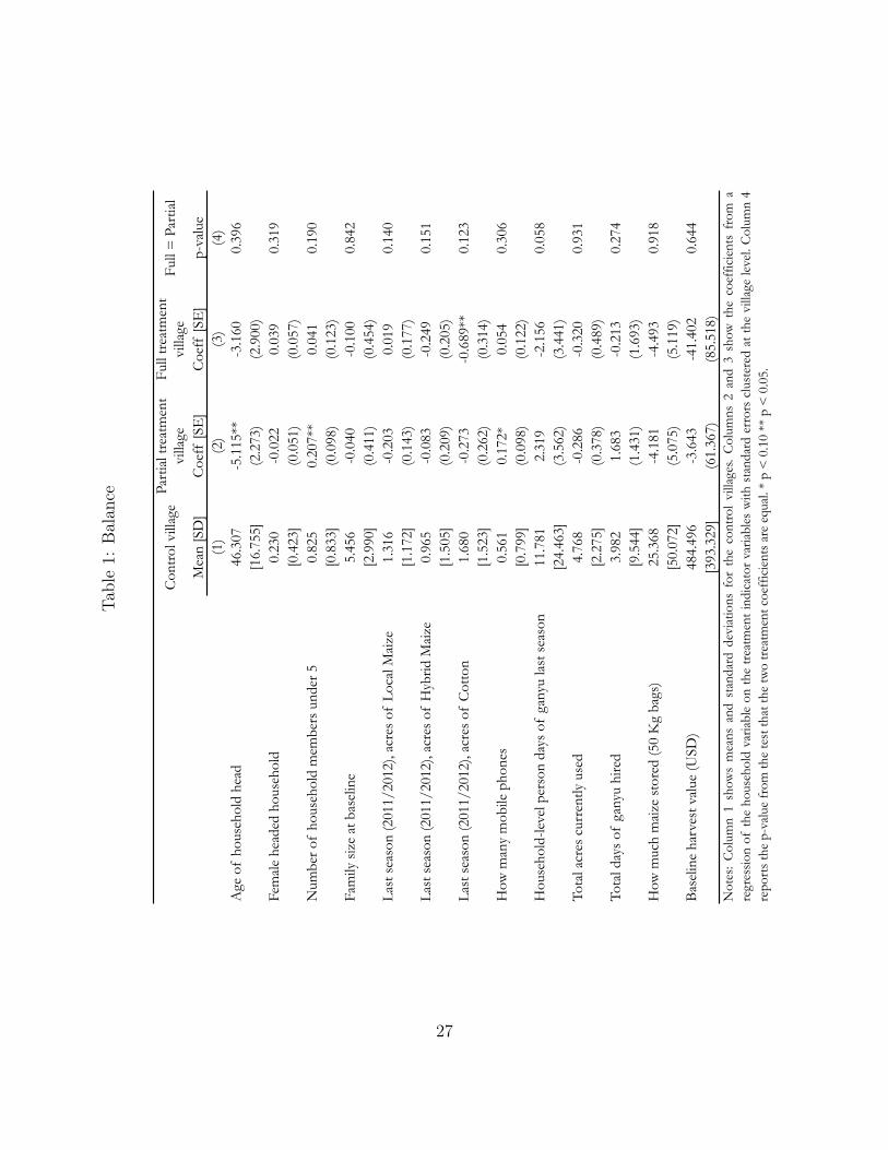
The coefficients presented in the subsequent analysis identify the causal effect of the loanunder the identifying assumption that treatment assignment is orthogonal to uiv. Table 1presents the means and standard deviations of baseline survey characteristics among studyhouseholds. Column 1 shows averages for control villages and columns 2 and 3 report thecoefficients from a regression of each household characteristic on treatment dummies, withstandard errors clustered at the village level. The significance of the coefficient represents thetest of the characteristic mean in each treatment against that in the control, while column

12For consistency, we define eligibility in both the full and the partial treatment villages conditional onattending the informational meeting.

14

4 shows the p-values from a test that the treatment coefficients are equal.A few of the summary statistics in Table 1 are worth noting. Household heads are around

46 years old and just under 25 percent are female. Households contain around 5.5 members,with around one child under 5. In the previous season, households produced 1.3 acres oflocal maize, 0.97 acres of hybrid maize and 1.7 acres of cotton on average, and used a totalof 4.8 acres for agricultural production. Households on average engaged in 12 days of casuallabor (ganyu) in the last season and hired around 4 days of ganyu. The average householdstored 25 bags of maize after the previous harvest and had a baseline harvest value of aroundUSD 484. With an average household size of more than 5 members and very limited incomebeyond agriculture, this means that virtually all households in our sample were well belowthe USD 1.25 per day per capita poverty threshold. In general, household characteristicsare well balanced, with 5 out of 39 pairwise tests significant at p < 0.10, which is just abovewhat we would expect from normal sampling with a 10 percent significance threshold. Mostnotably for our analysis, households in the full treatment villages engaged in marginallysignificantly fewer days of casual labor in the previous season than did households in thepartial treatment villages. Given the relatively small sample size and small imbalances, wecontrol for a full set of baseline characteristics throughout our analysis.

4.2 Attrition and selection

The main identifying assumption of our empirical analysis could be violated if householdsselect into eligibility status or drop out of the loan program differentially across treatments.Households could exit the study both during the midline survey and the endline survey.Overall attrition rates are low as shown in Table 2. The table reports means and standarddeviations at baseline in column 1 and the coefficients from a univariate regression of thebinary attrition or selection outcome on each explanatory variable with standard errorsclustered at the village level. Each coefficient therefore reflects a separate regression. Atotal of 439 households were enrolled into the study at baseline, 98 percent of whom were inthe midline and endline surveys. The probability of being in the midline and endline surveysis not affected by treatment status (columns 2 and 4).

Among households assigned to treatment, attrition could also occur at the stage of theloan meeting, which took place in each partial and full treatment village. Column 3 of Ta-ble 2 shows the probability of of attending the loan meeting as a function of each householdcharacteristic (again, each coefficient is its own regression), conditional on residing in a treat-

15

ment village and being in the baseline sample. Among eligible households, the probabilityof attending the loan meeting is increasing in the age of the household head and land size,but is not significantly affected by treatment intensity.

5 Results

We begin with descriptive statistics associated with take up and repayment of the loan, anda general manipulation test for changes in consumption, then move on to the analysis ofimpacts on labor supply. Then we investigate the equilibrium effect on wages, as describedin the conceptual framework (Section 2). We conclude our analysis with suggestive resultson within-village treatment spillovers.

5.1 Take up and repayment

Table 3 summarizes take up rates by treatment intensity. In the partial treatment villages,a total of 221 households were surveyed at baseline. 208 households participated in theinformation session, and 104 households were selected for participation in the loan programthrough the public lottery. All of the selected households decided to enroll in the loan pro-gram. Out of 104 households in the fully treated villages, 99 households came to the loaninformation session, and 90 households (91 percent) decided to sign up for the loan program.On average, households picked up 2.79 bags of maize flour in the partial treatment group(among eligible households), and 2.62 bags of maize flour in the full treatment group. Thehigh take up rate across treatments means that, in practice, our ITT estimates are closeapproximations of the average treatment effect on the treated. Though take up rates varyslightly with treatment intensity, they are not predicted by any of the household characteris-tics presented in Table 1 and the intention to treat estimation strategy mitigates remainingconcerns about selection into the loan.13

The bottom of Table 3 shows repayment rates, which were very high in both groups.Ninety-eight percent of participants repaid at least a part of the loan, and 95.2 and 97.7percent fully repaid their loans in the partial and full treatment villages, respectively. Nodifferences in repayment rates were found with respect to household size or financial resources(results not shown).

13The lottery itself may have affected take up rates by increasing the perceived value of the program byintroducing scarcity.

16

5.2 Consumption

As a first step toward identifying the impact of the loan program, we analyze food consump-tion. As described above, we conducted a midline survey in the middle of the hungry season,during which detailed information on food intake was collected. Maize is the most commonlygrown crop in Chipata District, and also the staple food in Zambia; well-off households con-sume maize in the form of a porridge (nshima) three times per day. To assess changes innutrition, we examine two summary measures of food consumption: the number of timesthe respondent reported eating nshima during the 24 hours preceding the interview, andwhether any family member had to skip a meal in the week preceding the interview becauseof food shortages. In the control group, the average respondent consumed nshima 1.74 timesin the 24 hours preceding the interview, and 36 percent report that a family member had tomiss a meal.

Table 4 shows the corresponding treatment effects. In full treatment villages, respon-dents consumed 0.2 more meals, an increase of 11 percent in eating frequency over thecontrol group. The increase in the partial treatment villages was smaller and not statisti-cally different from consumption in the control group. When we analyze the impact of loaneligibility at the household level in column 2, the overall effects appear smaller than the fullvillage treatment effect, but larger than the shifts observed in the partial treatment villages.We find similar impacts for the missed meals among family members. The probability ofmissing a meal was 16.5 percentage points lower in full treatment villages (a 45 percent re-duction relative to the control group); the average treatment effect was 6 percentage pointsin the partial treatment villages, but not statistically different from the control villages. Theindividual ITT is once again in between the partial and full treatment village impact.

5.3 Labor supply

We begin our analysis of labor supply effects with the midline survey. The main advantageof the midline survey is that recall was restricted to a two-week period preceding the survey(limiting recall issues), and that the timing of the survey (conducted in the last week ofFebruary and first week of March 2013) allows us to directly investigate labor shifts in themiddle of the hungry season, i.e. the most constrained part of the agricultural season.

Panel A of Table 5 shows the village level intention-to-treat results for household laborsupply at midline. In column (1) we analyze a binary indicator for whether the householdengaged in any off-farm ganyu labor activities. In the two-week period preceding the survey,

17

46 percent of households in the control group indicated that they provided ganyu labor onother farms.14 In full treatment villages, this proportion was reduced by 11.8 percentagepoints (25 percent), while the reduction in partial treatment villages was 7.6 percentagepoints (16.5 percent) and imprecisely estimated. Days of ganyu also decreased following asimilar pattern, though the treatment effect in the partial treatment villages is close to zero.While we find positive point estimates for labor supply on the the household farm in bothgroups (column 3), the confidence intervals are large and the effects are not statisticallysignificant. Finally, we observe no detectable change in hiring of outside labor (column 4).

In Panel B, we show the intention-to-treat results at the household level. The resultslook similar to Panel A: the estimated coefficient on ganyu provision (column 1) suggestsan average reduction in ganyu labor of 8 percentage points. Since we now also include non-eligible households in partial treatment areas (who may have benefited from the intervention)in the comparison category, the slightly smaller coefficient could in theory be evidence forspillover effects in these villages. At the household level, neither days of ganyu nor days onfarm (columns 2 and 3) are precisely estimated.

The main advantage of the midline data is its relatively short recall period with a pre-sumably more limited scope for recall bias. The longer recall period at endline allows usto investigate whether households compensated for lower rates of ganyu during the hungryseason with an increase before loan repayments were due. Table 6 shows results from theendline data, covering the full agricultural calendar, that are qualitatively similar to themidline results in Table 5. The probability of any off-farm labor at any point during theagricultural season falls by 9 percentage points in the fully treated villages relative to thecontrol. Days of ganyu fall, days of on-farm labor increase and days of hired labor increase infull treatment villages, all with coefficients that are large in magnitude (39 percent, 7 percentand 46 percent, respectively) but imprecisely estimated. Panel B shows the individual levelITT results, which is consistent with the midline outcomes. Because these measures alsoinclude the months preceding the loan offer, we also repeat the analysis in Appendix tableA.2, restricting outcomes to the months during which households had loans. This narroweranalysis requires that households accurately recall the timing of their labor decisions; per-

14The share of households in the control villages who report doing ganyu in the two weeks prior to themidline survey is substantially higher than the average ganyu rates reported for the previous February duringthe baseline survey. This can be attributed to two factors. First, the midline and baseline measures refer todifferent years, and ganyu rates may vary substantially from year to year. Second, the short recall periodin the midline survey may allow respondents to remember ganyu activities that they had forgotten in theintervening 8 months when asked at baseline about the previous February.

18

haps due to measurement error, estimates are consistent with but less precise than in Table6.

In our final set of results on labor supply, we focus on the period immediately precedingloan repayment and the endline survey. Column 4 of Table 6 shows the probability that ahousehold did any ganyu in the two months preceding loan repayment. Because the recallperiod in these questions is only two months, we expect the reports to be reasonably accurate.On average, in control village households, 29 percent of respondents report some ganyu intheir household in the two months prior to loan repayment. In full treatment villages, thatdrops by 13.8 percentage points (47.6 percent). The average effect on eligible households isa decrease of 8 percentage points.15

Additional analysis by gender using endline data suggests that treatment effects are largerfor female household members who have a lower baseline rate of ganyu (recall Figure 3). Infull treatment villages, the probability that a household supplies female ganyu fell by 6.8percentage points (p-value of 0.052) or by 29.3 percent, while the probability that a householdsupplies male ganyu fell by 3.7 percentage points (p-value of 0.50) or 7.8 percent. Note thatthese estimates assume equal probabilities of adult males and females able to supply laboracross treatment and control households.

5.4 Wages

As outlined in our theoretical framework, individual (or community) changes in ganyu laborparticipation should have only marginal effects on equilibrium wages if labor markets werenational or frictionless. As we have argued and shown above, workers’ ability to engage inshort-term labor opportunities beyond walking distance is somewhat limited, which meansthat large differentials between local labor market outcomes are likely.

To evaluate the wage impact of the loan programs, we start by analyzing wages reportedby households in the midline survey. As part of the midline survey, households were firstasked to report the total number of person-days of ganyu provided in the 2 weeks priorto the survey, and then asked to report total ganyu income for the household in total, aswell the days of ganyu worked and income earned by each household member. We start

15The lack of reported off-farm labor in the treatment villages preceding repayment are unlikely due toa lack of off-farm work opportunities. As shown in Appendix figure A.2, wages are high at harvest relativeto other times of the year. Labor supply is scarce, however, because most households are engaged on theirown land. At baseline, households reported a total of 64 person-days of ganyu during the harvest. Forcomparison, 232 person-days of ganyu were reported during weeding, 57 during planting and 199 during fieldpreparation.

19

our analysis by looking at the average wage reported at the household level: the totalganyu income divided by the total number of person-days reported. Two things are worthhighlighting. First, the duration of a typical ganyu work day varies substantially; the wagenumber calculated should thus be interpreted as the wage income a worker receives for atypical day of ganyu. Second, a substantial fraction of households do not do any ganyu, forwhich this variable is not defined; wages thus do not represent wage offers, but only wageoffers accepted.

Panel A of Table 7 shows that average wage rates reported at midline were around KR9.65, which corresponds to slightly less than USD 2 at 2013 exchange rates. In column 1we regress reported wages on the two treatment arms; in column 2 we use the fraction offarmers eligible for the program at the village level. Independent of the chosen specification,the magnitude of the observed effect is large, suggesting an increase of local wages of up to49 percent. The analysis is repeated in columns 3 and 4, using reported wages (total ganyu

income divided by total days worked) for each individual in the household who did ganyu.The individual-level wage is lower, on average, and the treatment effects are less preciselyestimated. We show the full distribution of reported wages at midline, by treatment arm, inAppendix figure A.3.

In the baseline and endline surveys, households were also asked to indicate the totalnumber of person-days worked off-farm over the agricultural season. For this longer-termrecall module, households were asked to separately report off-farm labor activities for eachof the four main parts of the agricultural season: field preparation, planting, weeding, andharvesting. Respondents indicated the total number of (full-time) person-days for eachactivity, as well as the total remuneration earned by the household, including food as well asother in-kind services. As Panel B of Table 7 shows, the average wage of KR 18 (USD 3.5)was substantially higher at endline than at midline. The higher rates observed in the endlinesurvey reflect seasonal variation in wages, as well as potentially longer working hours.

In Panel B of Table 7, we show the results of a basic household-level panel model, whereeach observation corresponds to a wage reported in a given season (2011/12 in baseline,2012/12 in endline) and for a given activity. A total of 1025 ganyu wages were reportedacross the two seasons. In Panel B of Table 7, we show the results from a basic difference-in-difference estimator with village fixed effects, where all activities in the year of the interven-tion are considered treated in villages with loan programs (columns 1 and 2). In columns 3and 4, we report the results of an alternative specification, where we only consider weedingand harvesting related activities in the second year as treated. Given that the vast majority

20

of ganyu activities fall in this category, the results from the two models are relatively simi-lar. All of the estimated coefficients go in the expected (positive) direction, but the standarderrors are large and coefficients are statistically insignificant. While the magnitudes of thewage treatment effects are (insignificantly) larger at endline than at midline, relative to therespective control group means, they are smaller (27-35 percent versus 49 percent). Thisdifference in the relative shift is due in part to the higher control group average observed atendline, but also perhaps to a dissipation of the treatment effect. Finally, as in the laboranalysis, we expect measurement error to be larger at endline than at midline.

The observed wage effects may be driven by adjustment on multiple margins. First, thenumber of households supplying labor to the market falls as a result of the intervention, asshown above. Second, the composition of individuals in the market also adjusts; in particular,as described in Section 5.3 above, female labor supply falls disproportionately. Finally, to theextent that the consumption gains shown above translate into better nutrition, productivitymay also increase, conditional on working in the labor market. We cannot disentangle thesedifferent channels, but the presence of all three helps explain the magnitudes of the wageeffects that we observe. In addition, our focus on small villages means that a relatively largefraction of the total village population is treated, producing a substantial shock to aggregatelabor supply.

5.5 Within-village spillovers

The results shown in Sections 5.2 and 5.3 suggest that ITT effects are smaller in partialtreatment villages than in the full treatment villages. To investigate the spillovers associatedwith the loan program, we separately estimate treatment effects for eligible and ineligiblehouseholds in partial treatment villages. We investigate three possible spillover channels:first, eligible households may share some of the additional resources by transferring foodto ineligible households or family members as gifts or on a loan basis. Second, eligiblehouseholds may hire more ineligible households to do ganyu. Third, general equilibrium wageeffects may impact labor allocation decisions of ineligible households in partial treatmentvillages, as described in Section 2.

Figure 4 and Appendix table A.3 show spillover effects on labor and consumption out-comes and on inter-household transfers, respectively. First, transfers from eligible to in-eligible households did not increase (Appendix table A.3). Interestingly, the likelihood ofhouseholds reporting incoming gifts and loans is substantially higher among eligible house-

21

holds, which is likely a reflection of eligible households reporting the maize loan programunder this category. Second, ganyu by ineligible households did not increase (Panels c andd of Figure 4), which is consistent with the observations that eligible households in par-tial treatment villages did not increase hiring (not shown). While we lack the precision todetect spillover effects at conventional levels of significance, Figure 4 shows that ineligiblehouseholds experience outcomes that move toward the treatment effects and away from thecontrols for consumption and labor impact. The graphs plot marginal effects from the inter-action of household-level eligibility and village-level treatment interactions. A comparisonacross ineligible households in pure control and partial villages shows the spillover effect onineligible households of being in a village where some households receive loans. A comparisonacross eligible households in partial and full treatment households shows the spillover impacton eligible households. In all panels of the figure, the effects are statistically indistinguish-able for eligible and ineligible in partial treatment villages. Conceptually, and based on themodel developed in Section 2, these results are consistent with income effects: for a givenamount of off farm labor, higher wages relax the consumption constraint of even ineligiblehouseholds. Given the very small number of clusters, all of these estimates are imprecise;larger studies will be needed to more closely identify local labor market spillovers.

6 Discussion and Conclusions

We implemented a simple and potentially scalable maize loan program in rural Zambia toidentify the effect of increased access to seasonal credit on off-farm labor supply. The resultsof the experiment suggest that additional access to short-term credit increases food con-sumption, decreases off-farm labor and increases local wages in targeted communities. Eventhough the intervention was relatively simple in its design, increased resource availabilityduring the growing season can potentially affect labor market outcomes through multiplemechanisms. First, short-term credit lowers the degree to which consumption-constrainedfarmers depend on short-term labor income, reducing local labor supply from particularlyresource-limited households. Second, improved nutrition potentially allows household mem-bers to work longer and harder (as in Strauss 1986), which may positively affect productivityon their own farm as well as for external labor activities. Both effects will be associated withincreases in local wages, which will in return also change the composition of the ganyu work-force from individuals engaging in ganyu primarily to smooth consumption to individualsengaging in ganyu activities to maximize the household’s net income.

22

Even though the credit program was designed to be broadly consistent with local creditmarket conditions, the extremely high uptake and repayment rates could be seen as evidencethat the loan program was considered financially beneficial, and thus provided a net transferto households. Given the high variability of local short-term lending rates reported, it ishard to quantify how large of a net transfer the loan program offered. With a maximumloan size of USD 27 and a market value of the repaid maize between USD 30 and USD 45(depending on the buyer), large net transfers seem unlikely. At an annual interest rate of100 percent, and assuming that the maize would have been sold cheaply in the absence ofthe program ($30), the estimated net transfer over the four-months loan period would beapproximately USD 3, which corresponds to about one day of ganyu income. In comparison,the labor responses seem rather large. At the mean, our results suggest that households areforgoing around KR 72 (~ USD 14) of ganyu income as a result of their reallocation awayfrom off-farm labor, which makes it seem unlikely that income effects would have driven theobserved shifts in labor allocation. In our view, the empirical patterns observed are mostconsistent with loan programs easing consumption-constraints for the households with thesmallest food or financial reserves. This fits well with the positive correlation between missedmeals and ganyu labor at midline, in both treatment and control villages.

Overall, our findings suggest that credit constraints affect consumption choices made byfarming households, and also distort farming households’ labor allocation decisions. Thisimplies that expanding seasonal credit to small farmers may allow them to optimize theirlabor allocation and to benefit from increased local wages. The rise in wages generated byincreased access to credit would lead to a redistribution of income from net buyers to netsellers of ganyu.

From a policy perspective, short-term loans may potentially be able to improve aggregateproductivity; our results suggest that repayment rates can be high enough to make suchprograms possible and sustainable in good years; in bad years - with large aggregate weatheror pest shocks - large drops in repayment rates seem likely; the addition of higher levelinsurance mechanisms may be necessary to ensure the financial stability and viability ofsuch programs over time. Ongoing data collection at a substantially larger scale will allowus to examine the extent to which the reallocation of labor resources to farmers’ own land canincrease the productivity of small-scale farmers and will track both sides of the labor marketto generate a more complete picture of the overall welfare implications of the intervention.

23

References

Basu, Karna and Maisy Wong, “Evaluating seasonal food security programs in EastIndonesia,” Mimeo, 2012.

Behrman, Jere R, Andrew D Foster, and Mark R Rosenzweig, “The dynamicsof agricultural production and the calorie-income relationship: Evidence from Pakistan,”Journal of Econometrics, 1997, 77 (1), 187–207.

Besley, Timothy, Savings, credit and insurance Handbook of Development Economics,North Holland, 1995.

Bruhn, Miriam and David McKenzie, “In Pursuit of Balance: Randomization inPractice in Development Field Experiments,” American Economic Journal: Applied Eco-

nomics, 2009, pp. 200–232.Bryan, G., S. Chowdhury, and A.M. Mobarak, “Seasonal Migration and Risk Aver-

sion,” Mimeo, 2013.Bryceson, Deborah Fahy, “Ganyu casual labour, famine and HIV/AIDS in rural Malawi:

causality and casualty,” Journal of Modern African Studies, 2006, 44 (2), 173.Burke, Marshall, “Selling low and buying high: An arbitrage puzzle in Kenyan villages,”

Mimeo, 2014.Chaudhuri, Shubham and Christina Paxson, “Smoothing consumption under income

seasonality: Buffer stocks vs. credit markets,” Mimeo, 2002.Cole, Steven M and Parakh N Hoon, “Piecework (Ganyu) as an Indicator of Household

Vulnerability in Rural Zambia,” Ecology of food and nutrition, 2013, 52 (5), 407–426.Dercon, Stefan and Pramila Krishnan, “Vulnerability, seasonality and poverty in

Ethiopia,” The Journal of Development Studies, 2000, 36 (6), 25–53.Dupas, Pascaline and Jonathan Robinson, “The Daily Grind: Cash Needs, Labor

Supply and Self-Control,” Mimeo, 2014.Fafchamps, Marcel, “Sequential labor decisions under uncertainty: An estimable house-

hold model of West-African farmers,” Econometrica, 1993, 61 (5), 1173–1197.Fink, Günther and Felix Masiye, “Assessing the impact of scaling-up bednet coverage

through agricultural loan programmes: evidence from a cluster randomised controlled trialin Katete, Zambia,” Transactions of the Royal Society of Tropical Medicine and Hygiene,2012, 106 (11), 660–667.

Goldberg, Jessica, “Kwacha gonna do? Experimental evidence about labor supply in ruralMalawi,” Mimeo, 2013.

24

Guiteras, Raymond and B. Kelsey Jack, “Incentives, Productivity and Selection inLabor Markets: Evidence from Rural Malawi,” Mimeo, 2014.

Ito, Takahiro and Takashi Kurosaki, “Weather risk, wages in kind, and the off-farmlabor supply of agricultural households in a developing country,” American Journal of

Agricultural Economics, 2009, 91 (3), 697–710.Jayachandran, Seema, “Selling labor low: Wage responses to productivity shocks in de-

veloping countries,” Journal of Political Economy, 2006, 114 (3), 538–575.Kerr, Rachel Bezner, “Informal Labor and Social Relations in Northern Malawi: The The-

oretical Challenges and Implications of Ganyu Labor for Food Security,” Rural sociology,2005, 70 (2), 167–187.

Khandker, Shahidur R, “Seasonality of income and poverty in Bangladesh,” Journal of

Development Economics, 2012, 97 (2), 244–256.Kochar, Anjini, “Explaining household vulnerability to idiosyncratic income shocks,” The

American Economic Review, 1995, pp. 159–164., “Smoothing consumption by smoothing income: Hours-of-work responses to idiosyncraticagricultural shocks in rural India,” Review of Economics and Statistics, 1999, 81 (1), 50–61.

Michaelowa, Katharina, Ralitza Dimova, and Anke Weber, “Ganyu Labour inMalawi: Understanding Rural Household’s Labour Supply Strategies,” Mimeo, 2010.

Mobarak, Ahmed Mushfiq and Mark Rosenzweig, “Risk, Insurance and Wages inGeneral Equilibrium,” Mimeo, 2014.

Morduch, Jonathan, “Income smoothing and consumption smoothing,” Journal of Eco-

nomic Perspectives, 1995, 9, 103–103.Orr, Alastair, Blessings Mwale, and Donata Saiti-Chitsonga, “Exploring seasonal

poverty traps: the ’six-week window’ in southern Malawi,” The Journal of Development

Studies, 2009, 45 (2), 227–255.Paxson, Christina H, “Consumption and income seasonality in Thailand,” Journal of

Political Economy, 1993, 101 (1), 39.Pitt, M. M. and M.R. Rosenzweig, Agricultural prices, food consumption and the health

and productivity of Indonesian farmers, Baltimore: Johns Hopkins University Press, 1986.Pitt, Mark M, Mark R Rosenzweig, and Md Nazmul Hassan, “Productivity, health,

and inequality in the intrahousehold distribution of food in low-income countries,” Amer-

ican Economic Review, 1990, 80 (5), 1139–1156.Ricker-Gilbert, Jacob, Nicole M Mason, Francis A Darko, and Solomon T Tembo,

“What are the effects of input subsidy programs on maize prices? Evidence from Malawi

25

and Zambia,” Agricultural Economics, 2013, 44 (6), 671–686.Rose, Elaina, “Ex ante and ex post labor supply response to risk in a low-income area,”

Journal of Development Economics, 2001, 64 (2), 371–388.Rosenzweig, Mark R, Handbook of Development Economics, Vol. 1, Elsevier,

and Hans P Binswanger, “Wealth, Weather Risk and the Composition and Profitabilityof Agricultural Investments,” Economic Journal, 1993, 103 (416), 56–78.

Schofield, Heather, “The Economic Costs of Low Caloric Intake: Evidence from India,”Mimeo, 2013.

Strauss, John, “Does better nutrition raise farm productivity?,” The Journal of Political

Economy, 1986, pp. 297–320.and Duncan Thomas, “Health, nutrition, and economic development,” Journal of Eco-

nomic Literature, 1998, 36 (2), 766–817.Subramanian, Shankar and Angus Deaton, “The demand for food and calories,” Jour-

nal of Political Economy, 1996, pp. 133–162.Zambian Central Statistics Office (CSO), “2010 Census of Population,” Government of

the Republic of Zambia, 2010.

26

Tabl

e1:

Bal

ance

Con

trol

vill

age

Part

ial t

reat

men

t vi

llage

Full

trea

tmen

t vi

llage

Full

= P

artia

l

Mea

n [S

D]

Coe

ff [S

E]

Coe

ff [S

E]

p-va

lue

(1)

(2)

(3)

(4)

Age

of

hous

ehol

d he

ad46

.307

-5.1

15**

-3.1

600.

396

[16.

755]

(2.2

73)

(2.9

00)

Fem

ale

head

ed h

ouse

hold

0.23

0-0

.022

0.03

90.

319

[0.4

23]

(0.0

51)

(0.0

57)

Num

ber o

f ho

useh

old

mem

bers

und

er 5

0.

825

0.20

7**

0.04

10.

190

[0.8

33]

(0.0

98)

(0.1

23)

Fam

ily s

ize

at b

asel

ine

5.45

6-0

.040

-0.1

000.

842

[2.9

90]

(0.4

11)

(0.4

54)

Last

sea

son

(201

1/20

12),

acre

s of

Loc

al M

aize

1.31

6-0

.203

0.01

90.

140

[1.1

72]

(0.1

43)

(0.1

77)

Last

sea

son

(201

1/20

12),

acre

s of

Hyb

rid M

aize

0.96

5-0

.083

-0.2

490.

151

[1.5

05]

(0.2

09)

(0.2

05)

Last

sea

son

(201

1/20

12),

acre

s of

Cot

ton

1.68

0-0

.273

-0.6

89**

0.12

3[1

.523

](0

.262

)(0

.314

)H

ow m

any

mob

ile p

hone

s0.

561

0.17

2*0.

054

0.30

6[0

.799

](0

.098

)(0

.122

)H

ouse

hold

-leve

l per

son

days

of

gany

u la

st s

easo

n11

.781

2.31

9-2

.156

0.05

8[2

4.46

3](3

.562

)(3

.441

)To

tal a

cres

cur

rent

ly u

sed

4.76

8-0

.286

-0.3

200.

931

[2.2

75]

(0.3

78)

(0.4

89)

Tota

l day

s of

gan

yu h

ired

3.98

21.

683

-0.2

130.

274

[9.5

44]

(1.4

31)

(1.6

93)

How

muc

h m

aize

sto

red

(50

Kg

bags

)25

.368

-4.1

81-4

.493

0.91

8[5

0.07

2](5

.075

)(5

.119

)B

asel

ine

harv

est v

alue

(USD

)48

4.49

6-3

.643

-41.

402

0.64

4[3

93.3

29]

(61.

367)

(85.

518)

Not

es:

Col

umn

1sh

ows

mea

nsan

dst

anda

rdde

viat

ions

for

the

cont

rol

villa

ges.

Col

umns

2an

d3

show

the

coef

ficie

nts

from

are

gres

sion

ofth

eho

useh

old

varia

ble

onth

etr

eatm

ent

indi

cato

rva

riabl

esw

ithst

anda

rder

rors

clus

tere

dat

the

villa

gele

vel.

Col

umn

4re

port

s th

e p-

valu

e fr

om th

e te

st th

at th

e tw

o tr

eatm

ent c

oeff

icie

nts

are

equa

l. *

p <

0.1

0 **

p <

0.0

5.

27

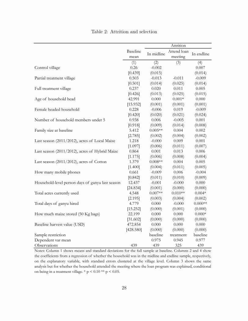
Table 2: Attrition and selection

Baseline mean In midline Attend loan

meeting In endline

(1) (2) (3) (4) Control village 0.26 -0.002 0.007

[0.439] (0.015) (0.014)Partial treatment village 0.503 -0.013 -0.011 -0.009

[0.501] (0.014) (0.025) (0.014)Full treatment village 0.237 0.020 0.011 0.005

[0.426] (0.013) (0.025) (0.015)Age of household head 42.991 0.000 0.001* 0.000

[15.932] (0.001) (0.001) (0.001)Female headed household 0.228 -0.006 0.019 -0.009

[0.420] (0.020) (0.021) (0.024)Number of household members under 5 0.938 0.006 -0.005 0.001

[0.918] (0.009) (0.014) (0.008)Family size at baseline 5.412 0.005** 0.004 0.002

[2.785] (0.002) (0.004) (0.002)Last season (2011/2012), acres of Local Maize 1.218 -0.000 0.009 0.001

[1.097] (0.006) (0.011) (0.007)Last season (2011/2012), acres of Hybrid Maize 0.864 0.001 0.013 0.006

[1.175] (0.006) (0.008) (0.004)Last season (2011/2012), acres of Cotton 1.379 0.008** 0.004 0.005

[1.400] (0.004) (0.011) (0.005)How many mobile phones 0.661 -0.009 0.006 -0.004

[0.842] (0.011) (0.010) (0.009)Household-level person days of ganyu last season 12.437 -0.001 -0.000 0.000

[24.834] (0.001) (0.000) (0.000)Total acres currently used 4.548 0.007** 0.010** 0.004*

[2.195] (0.003) (0.004) (0.002)Total days of ganyu hired 4.779 0.000 -0.000 0.000**

[15.252] (0.000) (0.001) (0.000)How much maize stored (50 Kg bags) 22.199 0.000 0.000 0.000*

[31.602] (0.000) (0.000) (0.000)Baseline harvest value (USD) 472.854 0.000 0.000 0.000

[428.580] (0.000) (0.000) (0.000)Sample restriction baseline treatment baselineDependent var mean 0.975 0.945 0.977Observations 439 439 325 439

Attrition

Notes: Column 1 shows means and standard deviations for the full sample at baseline. Columns 2 and 4 showthe coefficients from a regression of whether the household was in the midline and endline sample, respectively,on the explanatory variable, with standard errors clustered at the village level. Column 3 shows the sameanalysis but for whether the household attended the meeting where the loan program was explained, conditionalon being in a treatment village. * p < 0.10 ** p < 0.05.

28

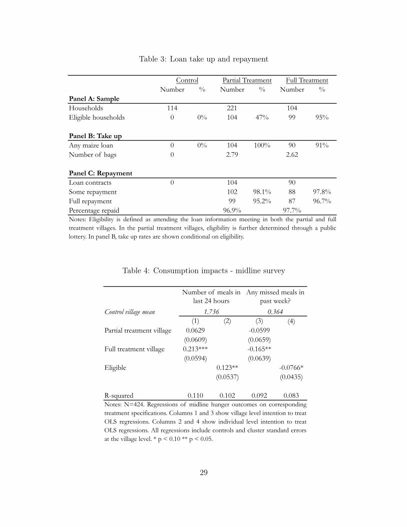
Table 3: Loan take up and repayment

Number % Number % Number %Panel A: SampleHouseholds 114 221 104Eligible households 0 0% 104 47% 99 95%

Panel B: Take upAny maize loan 0 0% 104 100% 90 91%Number of bags 0 2.79 2.62

Panel C: RepaymentLoan contracts 0 104 90Some repayment 102 98.1% 88 97.8%Full repayment 99 95.2% 87 96.7%Percentage repaid 96.9% 97.7%

Control Partial Treatment Full Treatment

Notes: Eligibility is defined as attending the loan information meeting in both the partial and fulltreatment villages. In the partial treatment villages, eligibility is further determined through a publiclottery. In panel B, take up rates are shown conditional on eligibility.

Table 4: Consumption impacts - midline survey

Control village mean(1) (2) (3) (4)

Partial treatment village 0.0629 -0.0599(0.0609) (0.0659)

Full treatment village 0.213*** -0.165**(0.0594) (0.0639)

Eligible 0.123** -0.0766*(0.0537) (0.0435)

R-squared 0.110 0.102 0.092 0.083

Number of meals in last 24 hours

Any missed meals in past week?

Notes: N=424. Regressions of midline hunger outcomes on correspondingtreatment specifications. Columns 1 and 3 show village level intention to treatOLS regressions. Columns 2 and 4 show individual level intention to treatOLS regressions. All regressions include controls and cluster standard errorsat the village level. * p < 0.10 ** p < 0.05.

1.736 0.364

29

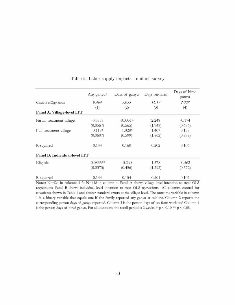
Table 5: Labor supply impacts - midline survey

Any ganyu? Days of ganyu Days on-farm Days of hired ganyu

Control village mean 0.464 3.055 16.17 2.009(1) (2) (3) (4)

Panel A: Village-level ITT

Partial treatment village -0.0757 -0.00514 2.248 -0.174(0.0567) (0.565) (1.948) (0.686)

Full treatment village -0.118* -1.028* 1.407 0.158(0.0607) (0.599) (1.862) (0.878)

R-squared 0.144 0.160 0.202 0.106

Panel B: Individual-level ITT

Eligible -0.0835** -0.260 1.578 -0.562(0.0373) (0.456) (1.292) (0.572)

R-squared 0.144 0.154 0.201 0.107Notes: N=424 in columns 1-3; N=418 in column 4. Panel A shows village level intention to treat OLSregressions. Panel B shows individual level intention to treat OLS regressions. All columns control forcovariates shown in Table 1 and cluster standard errors at the village level. The outcome variable in column1 is a binary variable that equals one if the family reported any ganyu at midline. Column 2 reports thecorresponding person-days of ganyu reported. Column 3 is the person-days of on-farm work and Column 4is the person-days of hired ganyu. For all questions, the recall period is 2 weeks. * p < 0.10 ** p < 0.05.

30

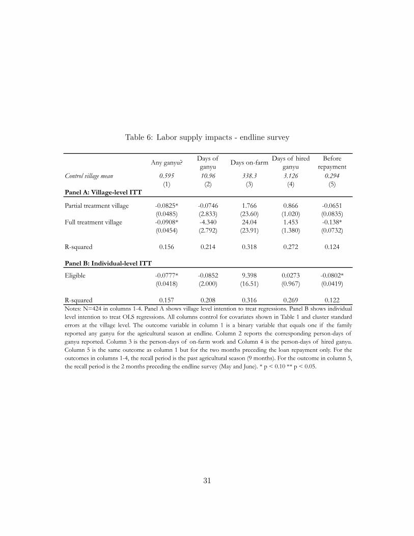
Table 6: Labor supply impacts - endline survey

Any ganyu? Days of ganyu Days on-farm Days of hired

ganyuBefore

repaymentControl village mean 0.595 10.96 338.3 3.126 0.294

(1) (2) (3) (4) (5)Panel A: Village-level ITT

Partial treatment village -0.0825* -0.0746 1.766 0.866 -0.0651(0.0485) (2.833) (23.60) (1.020) (0.0835)

Full treatment village -0.0908* -4.340 24.04 1.453 -0.138*(0.0454) (2.792) (23.91) (1.380) (0.0732)

R-squared 0.156 0.214 0.318 0.272 0.124

Panel B: Individual-level ITT

Eligible -0.0777* -0.0852 9.398 0.0273 -0.0802*(0.0418) (2.000) (16.51) (0.967) (0.0419)

R-squared 0.157 0.208 0.316 0.269 0.122Notes: N=424 in columns 1-4. Panel A shows village level intention to treat regressions. Panel B shows individuallevel intention to treat OLS regressions. All columns control for covariates shown in Table 1 and cluster standarderrors at the village level. The outcome variable in column 1 is a binary variable that equals one if the familyreported any ganyu for the agricultural season at endline. Column 2 reports the corresponding person-days ofganyu reported. Column 3 is the person-days of on-farm work and Column 4 is the person-days of hired ganyu.Column 5 is the same outcome as column 1 but for the two months preceding the loan repayment only. For theoutcomes in columns 1-4, the recall period is the past agricultural season (9 months). For the outcome in column 5,the recall period is the 2 months preceding the endline survey (May and June). * p < 0.10 ** p < 0.05.

31

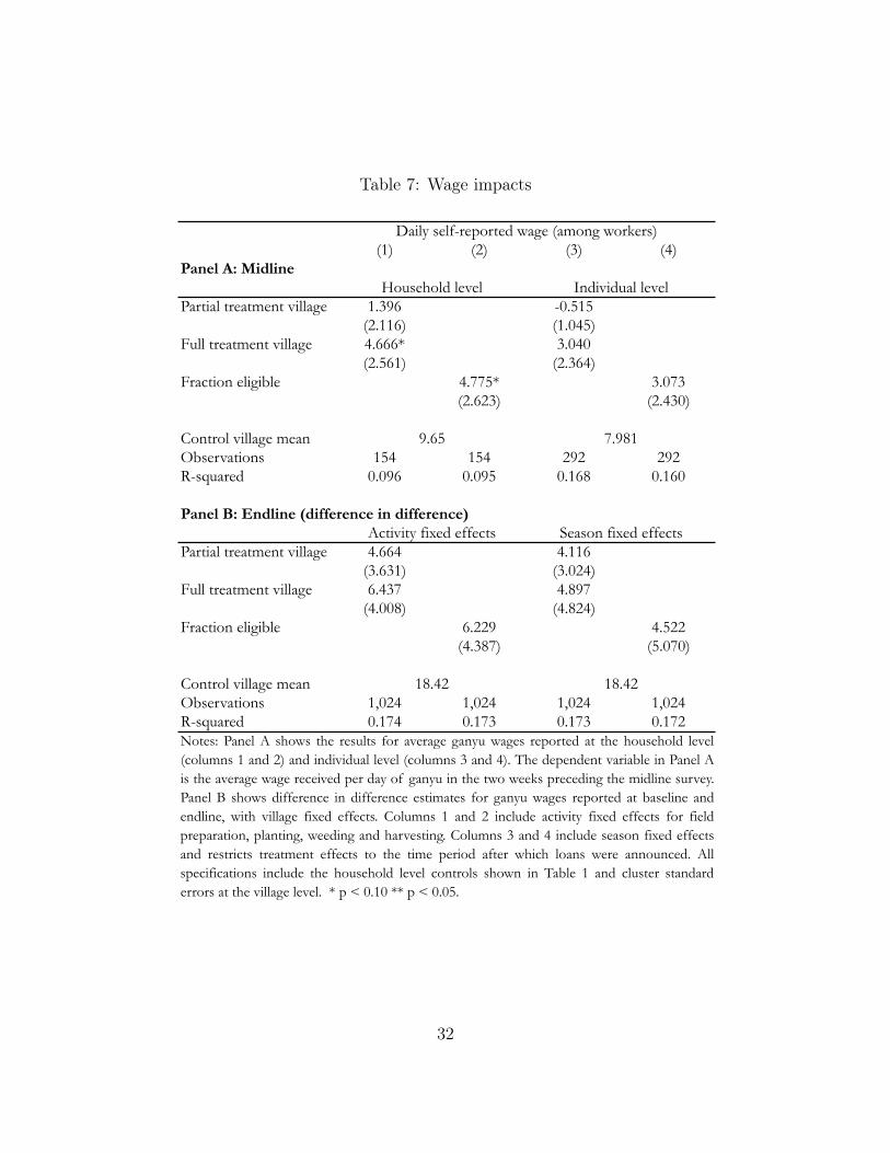
Table 7: Wage impacts

(1) (2) (3) (4)Panel A: Midline

Partial treatment village 1.396 -0.515(2.116) (1.045)

Full treatment village 4.666* 3.040(2.561) (2.364)

Fraction eligible 4.775* 3.073(2.623) (2.430)

Control village meanObservations 154 154 292 292R-squared 0.096 0.095 0.168 0.160

Panel B: Endline (difference in difference)

Partial treatment village 4.664 4.116(3.631) (3.024)

Full treatment village 6.437 4.897(4.008) (4.824)

Fraction eligible 6.229 4.522(4.387) (5.070)

Control village meanObservations 1,024 1,024 1,024 1,024R-squared 0.174 0.173 0.173 0.172Notes: Panel A shows the results for average ganyu wages reported at the household level(columns 1 and 2) and individual level (columns 3 and 4). The dependent variable in Panel Ais the average wage received per day of ganyu in the two weeks preceding the midline survey.Panel B shows difference in difference estimates for ganyu wages reported at baseline andendline, with village fixed effects. Columns 1 and 2 include activity fixed effects for fieldpreparation, planting, weeding and harvesting. Columns 3 and 4 include season fixed effectsand restricts treatment effects to the time period after which loans were announced. Allspecifications include the household level controls shown in Table 1 and cluster standarderrors at the village level. * p < 0.10 ** p < 0.05.

Daily self-reported wage (among workers)

Household level Individual level

Activity fixed effects Season fixed effects

18.42 18.42

9.65 7.981

32

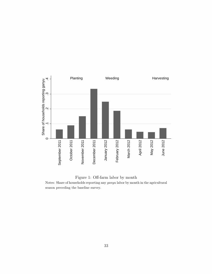
Planting Weeding Harvesting

0.1

.2.3

.4Sh

are

of h

ouse

hold

s re

porti

ng g

anyu

Sept

embe

r 201

1

Oct

ober

201

1

Nove

mbe

r 201

1

Dece

mbe

r 201

1

Janu

ary

2012

Febr

uary

201

2

Mar

ch 2

012

April

201

2

May

201

2

June

201

2

Figure 1: Off-farm labor by monthNotes: Share of households reporting any ganyu labor by month in the agriculturalseason preceding the baseline survey.

33

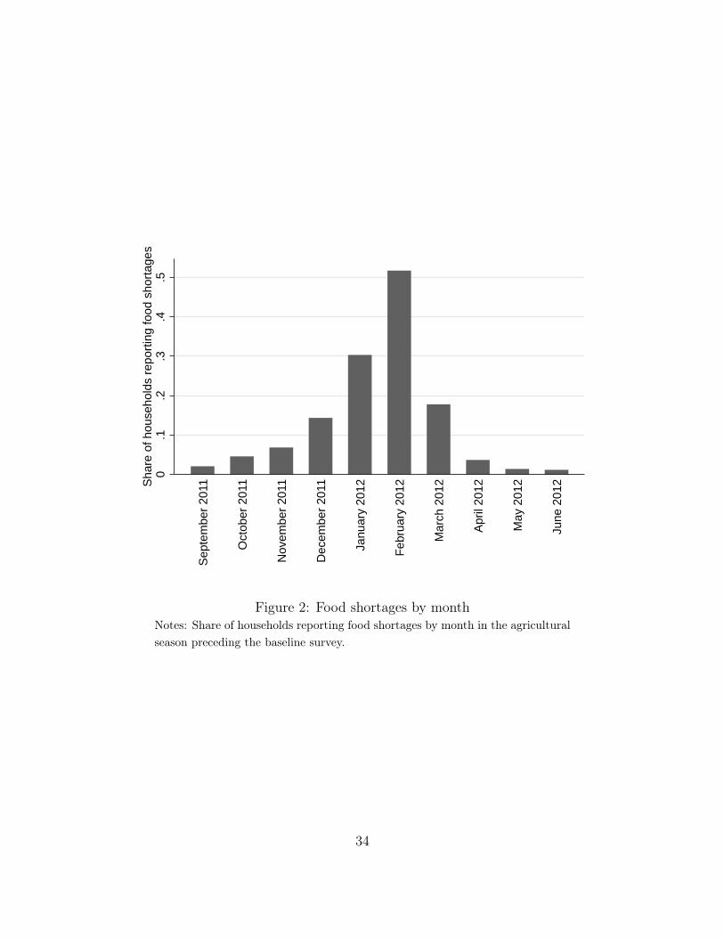
0.1

.2.3

.4.5

Shar

e of

hou

seho

lds

repo

rting

food

sho

rtage

s

Sept

embe

r 201

1

Oct

ober

201

1

Nove

mbe

r 201

1

Dece

mbe

r 201

1

Janu

ary

2012

Febr

uary

201

2

Mar

ch 2

012

April

201

2

May

201

2

June

201

2

Figure 2: Food shortages by monthNotes: Share of households reporting food shortages by month in the agriculturalseason preceding the baseline survey.

34

!"#

$!"#

%!"#

&!"#

'!"#

(!"#

)!"#

*!"#

$(+%'# %(+&'# &(+''# '(+('# ((,#

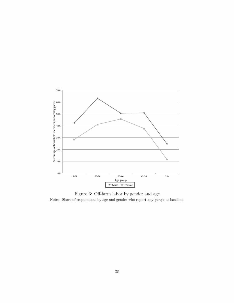
-./0.1

234.#56#7

589.75

:;#<

.<=.

/9#>./65/<

?14#431@8#

A4.#4/58>#

B3:.# C.<3:.#

Figure 3: Off-farm labor by gender and ageNotes: Share of respondents by age and gender who report any ganyu at baseline.

35

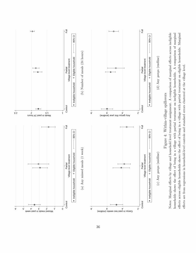
0.1.2.3.4.5.6Missed meals in past week

Cont

rol

Parti

alFu

llVi

llage

-leve

l tre

atm

ent

Inel

igib

le h

ouse

hold

Elig

ible

hou

seho

ld95

% C

I

(a)

Any

mis

sed

mea

ls(1

wee

k)

11.522.5Meals in past 24 hours

Cont

rol

Parti

alFu

llVi

llage

-leve

l tre

atm

ent

Inel

igib

le h

ouse

hold

Elig

ible

hou

seho

ld95

% C

I

(b)

Num

ber

ofm

eals

(24

hour

s)

.2.4.6.8Ganyu in past two weeks (midline)

Cont

rol

Parti

alFu

llVi

llage

-leve

l tre

atm

ent

Inel

igib

le h

ouse

hold

Elig

ible

hou

seho

ld95

% C

I

(c)

Any

gany

u(m

idlin

e)

.2.4.6.8Any ganyu this year (endline)

Cont

rol

Parti

alFu

llVi

llage

-leve

l tre

atm

ent

Inel

igib

le h

ouse

hold

Elig

ible

hou

seho

ld95

% C

I

(d)

Any

gany

u(e

ndlin

e)

Figu

re4:

With

in-v

illag

esp

illov

ers

Not

es:

Mar

gina

leffe

cts

byvi

llage

and

hous

ehol

dle

velt

reat

men

tas

sign

men

t.A

com

pari

son

ofm

argi

nale

ffect

sac

ross

inel

igib

leho

useh

olds

show

sth

eeff

ect

ofbe

ing

ina

villa

gew

ith

part

ial

trea

tmen

ton

inel

igib

leho

useh

olds

.A

com

pari

son

ofm

argi

nal

effec

tsac

ross

elig

ible

hous

ehol

dssh

ows

the

effec

tof

bein

gin

avi

llage

wit

hpa

rtia

ltre

atm

ent

onel

igib

leho

useh

olds

.M

argi

nal

effec

tsar

efr

omre

gres

sion

sin

hous

ehol

d-le

velc

ontr

ols

and

stan

dard

erro

rscl

uste

red

atth

evi

llage

leve

l.

36

Appendix

37

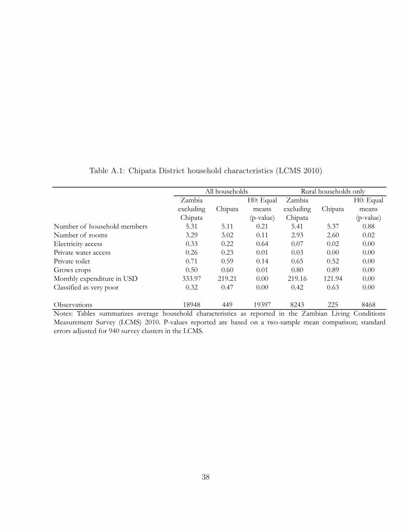
Table A.1: Chipata District household characteristics (LCMS 2010)

Zambia excluding Chipata

ChipataH0: Equal

means (p-value)

Zambia excluding Chipata

ChipataH0: Equal

means (p-value)

Number of household members 5.31 5.11 0.21 5.41 5.37 0.88Number of rooms 3.29 3.02 0.11 2.93 2.60 0.02Electricity access 0.33 0.22 0.64 0.07 0.02 0.00Private water access 0.26 0.23 0.01 0.03 0.00 0.00Private toilet 0.71 0.59 0.14 0.65 0.52 0.00Grows crops 0.50 0.60 0.01 0.80 0.89 0.00Monthly expenditure in USD 333.97 219.21 0.00 219.16 121.94 0.00Classified as very poor 0.32 0.47 0.00 0.42 0.63 0.00

Observations 18948 449 19397 8243 225 8468

All households Rural households only

Notes: Tables summarizes average household characteristics as reported in the Zambian Living ConditionsMeasurement Survey (LCMS) 2010. P-values reported are based on a two-sample mean comparison; standarderrors adjusted for 940 survey clusters in the LCMS.

38

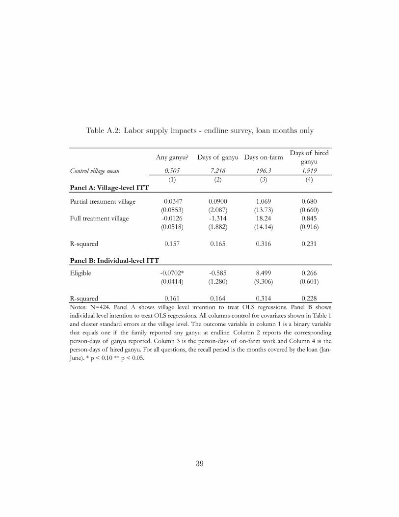
Table A.2: Labor supply impacts - endline survey, loan months only

Any ganyu? Days of ganyu Days on-farm Days of hired ganyu

Control village mean 0.505 7.216 196.3 1.919(1) (2) (3) (4)

Panel A: Village-level ITT

Partial treatment village -0.0347 0.0900 1.069 0.680(0.0553) (2.087) (13.73) (0.660)

Full treatment village -0.0126 -1.314 18.24 0.845(0.0518) (1.882) (14.14) (0.916)

R-squared 0.157 0.165 0.316 0.231

Panel B: Individual-level ITT

Eligible -0.0702* -0.585 8.499 0.266(0.0414) (1.280) (9.306) (0.601)

R-squared 0.161 0.164 0.314 0.228Notes: N=424. Panel A shows village level intention to treat OLS regressions. Panel B showsindividual level intention to treat OLS regressions. All columns control for covariates shown in Table 1and cluster standard errors at the village level. The outcome variable in column 1 is a binary variablethat equals one if the family reported any ganyu at endline. Column 2 reports the correspondingperson-days of ganyu reported. Column 3 is the person-days of on-farm work and Column 4 is theperson-days of hired ganyu. For all questions, the recall period is the months covered by the loan (Jan-June). * p < 0.10 ** p < 0.05.

39

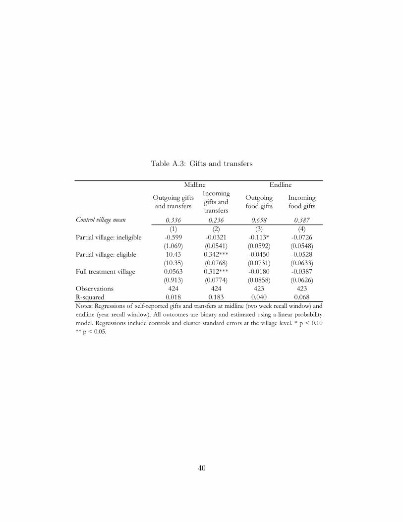
Table A.3: Gifts and transfers

Outgoing gifts and transfers

Incoming gifts and transfers

Outgoing food gifts

Incoming food gifts

Control village mean 0.336 0.236 0.658 0.387(1) (2) (3) (4)

Partial village: ineligible -0.599 -0.0321 -0.113* -0.0726(1.069) (0.0541) (0.0592) (0.0548)

Partial village: eligible 10.43 0.342*** -0.0450 -0.0528(10.35) (0.0768) (0.0731) (0.0633)

Full treatment village 0.0563 0.312*** -0.0180 -0.0387(0.913) (0.0774) (0.0858) (0.0626)

Observations 424 424 423 423R-squared 0.018 0.183 0.040 0.068

Midline Endline

Notes: Regressions of self-reported gifts and transfers at midline (two week recall window) andendline (year recall window). All outcomes are binary and estimated using a linear probabilitymodel. Regressions include controls and cluster standard errors at the village level. * p < 0.10** p < 0.05.

40

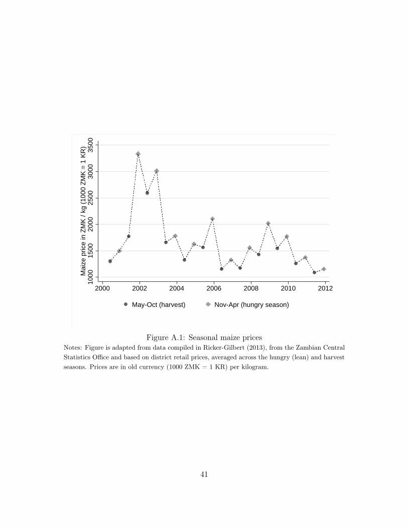
1000

1500

2000

2500

3000

3500

Mai

ze p

rice

in Z

MK

/ kg

(100

0 ZM

K =

1 KR

)

2000 2002 2004 2006 2008 2010 2012

May-Oct (harvest) Nov-Apr (hungry season)

Figure A.1: Seasonal maize pricesNotes: Figure is adapted from data compiled in Ricker-Gilbert (2013), from the Zambian CentralStatistics Office and based on district retail prices, averaged across the hungry (lean) and harvestseasons. Prices are in old currency (1000 ZMK = 1 KR) per kilogram.

41

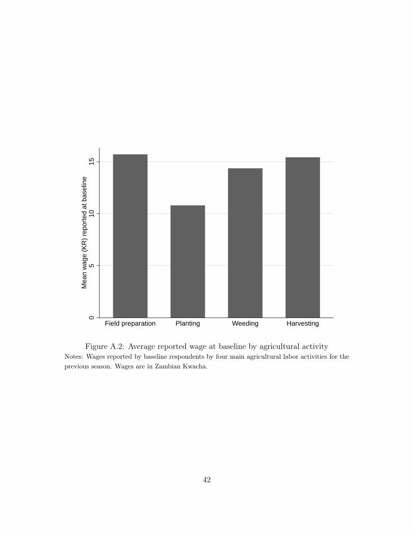
05

1015

Mea

n wa

ge (K

R) re

porte

d at

bas

elin

e

Field preparation Planting Weeding Harvesting

Figure A.2: Average reported wage at baseline by agricultural activityNotes: Wages reported by baseline respondents by four main agricultural labor activities for theprevious season. Wages are in Zambian Kwacha.

42

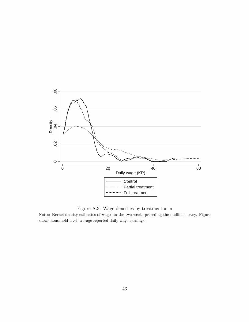
0.0

2.0

4.0

6.0

8De

nsity

0 20 40 60Daily wage (KR)

ControlPartial treatmentFull treatment

Figure A.3: Wage densities by treatment armNotes: Kernel density estimates of wages in the two weeks preceding the midline survey. Figureshows household-level average reported daily wage earnings.

43