W -L M -E Sugo/research/annrev.pdf5 Nov 2001 12:13 AR AR151-14.tex AR151-14.SGM ARv2(2001/05/10) P1: GJC 350 PIOMELLI ¥BALARAS In direct numerical simulations (DNS), on the other

5 Nov 2001 12:13 AR AR151-14.tex AR151-14.SGM ARv2(2001/05/10)P1: GJC

Annu. Rev. Fluid Mech. 2002. 34:349–74Copyright c© 2002 by Annual Reviews. All rights reserved

WALL-LAYER MODELS FOR

LARGE-EDDY SIMULATIONS

Ugo Piomelli and Elias BalarasDepartment of Mechanical Engineering, University of Maryland, College Park,Maryland 20742; e-mail: [email protected], [email protected]

Key Words large-eddy simulations, wall-layer models, approximate boundaryconditions

■ Abstract Because the cost of large-eddy simulations (LES) of wall-boundedflows that resolve all the important eddies depends strongly on the Reynolds num-ber, methods to bypass the wall layer are required to perform high-Reynolds-numberLES at a reasonable cost. In this paper the available methodologies are reviewed, andtheir ranges of applicability are highlighted. Various unresolved issues in wall-layermodeling are presented, mostly in the context of engineering applications.

1. INTRODUCTION

The decrease in the cost of computer power over the last few years has increasedthe impact of computational fluid dynamics. Numerical simulations of fluid flows,which until a few decades ago were confined to the research environment, are nowsuccessfully used for the development and design of engineering devices. Despitethe advances in computer speed and the algorithmic developments, however, thenumerical simulation of turbulent flows has not yet reached a mature stage: Noneof the techniques currently available can be reliably applied to all problems ofscientific or technological interest.

The solution of the Reynolds-averaged Navier-Stokes equations (RANS) isthe tool that is most commonly applied, especially in engineering applications,to the solution of turbulent flow problems. The RANS equations are obtainedby time- or ensemble-averaging the Navier-Stokes equations to yield a set oftransport equations for the averaged momentum. The effect of all the scales ofmotion is modeled. Models for the RANS equations have been the object of muchstudy over the last 30 years, but no model has emerged that gives accurate resultsin all flows without ad hoc adjustments of the model constants (see Wilcox 2001).This may be due to the fact that the large, energy-carrying eddies are much affectedby the boundary conditions, and universal models that account for their dynamicsmay be impossible to develop.

0066-4189/02/0115-0349$14.00 349


350 PIOMELLI ¥ BALARAS

In direct numerical simulations (DNS), on the other hand, all the scales ofmotion are resolved accurately, and no modeling is used. DNS is the most accuratenumerical method available at present but is limited by its cost: Because all scales ofmotion must be resolved, the number of grid points in each direction is proportionalto the ratio between the largest and the smallest eddy in the flow. This ratio isproportional toRe3/4

L (whereReL is the Reynolds number based on an integralscale of the flow). Thus, the number of points in three dimensions isNx NyNz ∝Re9/4

L . Present computer resources limit the application of DNS to flows withReL = o(104), and theRe3/4

L dependence of the number of grid points makes itunrealistic to expect that DNS can be used for high-Reengineering applications inthe near future. A recent review of DNS can be found in Moin & Mahesh (1998).

Large-eddy simulation is a technique intermediate between the solution of theRANS equations and DNS. In large-eddy simulation (LES) the large, energy-carrying eddies are computed, whereas only the small, subgrid scales of motionare modeled. LES can be more accurate than the RANS approach because thesmall scales tend to be more isotropic and homogeneous than the large ones, andthus more amenable to universal modeling. Furthermore, the modeled subgridscale (SGS) stresses only contribute a small fraction of the total turbulent stresses.Compared with DNS, LES does not suffer from the same strict resolution require-ments of DNS. Recent reviews of LES can be found in the articles by Mason(1994), Lesieur & Metais (1996), Piomelli (1999), and Meneveau & Katz (2000).

LES has received increased attention, in recent years, as a tool to study thephysics of turbulence in flows at higher Reynolds number, or in more complex ge-ometries, than DNS. Its most successful applications, however, have still been formoderate Reynolds numbers; examples include the flow inside an internal combus-tion engine (Verzicco et al. 2000) or the sound emission from the trailing edge ofa hydrofoil atRec= 2× 106 (Wang & Moin 2000). In a wide range of flows in thegeophysical sciences (especially in meteorology and oceanography) and engineer-ing (for instance, in ship hydrodynamics or in aircraft aerodynamics), however,the Reynolds number is very high, of the order of tens or hundreds of millions.The extension of LES that resolves the wall-layer structures (henceforth called“resolved LES”) to such flows has been less successful owing to the increased costof the calculations when a solid boundary is present.

The first complete analysis of grid-resolution requirements for LES of turbulentboundary layers can be found in the landmark paper by Chapman (1979). The flowin a flat-plate boundary layer or plane channel is generally divided into an innerlayer in which the effects of viscosity are important and an outer one in which thedirect effects of the viscosity on the mean velocity are negligible. Chapman (1979)examined the resolution requirements for inner and outer layers separately. In theouter layer in which the important eddies scale like the boundary-layer thicknessor the channel half-heightδ, he obtained an estimate for the outer-layer resolutionby integrating Pao’s (1965) energy spectrum and showed that the number of pointsin the wall-normal direction required to resolve a given fraction of the turbulentkinetic energy is essentially independent ofRe. Assuming that the grid size in


WALL-LAYER MODELS FOR LES 351

the streamwise and spanwise directions is a fixed fraction of the boundary-layerthickness (which varies approximately likeRe0.2) his estimate results in a totalnumber of grid points proportional toRe0.4. Chapman estimated that only 2500points are required to resolve a volumeδ

3of the flow, whereδ is an average

boundary-layer thickness. In actual calculations a wide range of resolutions isfound: In calculations of plane channel flow, for instance, Schumann (1979) usedbetween 128 and 4096 points to resolve a volumeδ3 (hereδ is the channel half-height), whereas Piomelli et al. (1989) used 1000 points.

The resolution of the inner layer is much more demanding: Its dynamics aredominated by quasi-streamwise vortices (see the review by Robinson 1991) whosedimensions are constant in wall units (i.e., when normalized with the kinematicviscosityν and the friction velocityuτ = (τw/ρ)1/2, whereτw is the wall stress andρ the fluid density). If the inner-layer eddies are resolved, a constant grid spacingin wall units must be used. In a boundary layer or channel flow, this requirementresults in streamwise and spanwise grid sizes1x+ ' 100,1z+ ' 20 (where wallunits are defined asx+i = xi uτ /ν). As the outer flow is approached, however, largergrid spacings can be used. An optimal computation, therefore, would use nestedgrids, with1x+ and1z+ increasing as one moves away from the wall. Underthese conditions, Chapman (1979) estimated that the number of points required toresolve the viscous sublayer is

(Nx NyNz)vs ∝ C f Re2L, (1)

which, assumingC f ∝ Re−0.2L , gives

(Nx NyNz)vs ∝ Re1.8L . (2)

In plane channel flow (an important test case for numerical simulations)Chapman’s (1979) estimate for the cost of the outer layer needs to be modified.The size of the largest eddies is determined by the channel height and is not afunction of the Reynolds number, whereas the cost of resolving the inner layeris the same for channels and boundary layers. Grid-resolution estimates for morecomplex flows cannot be derived a priori.

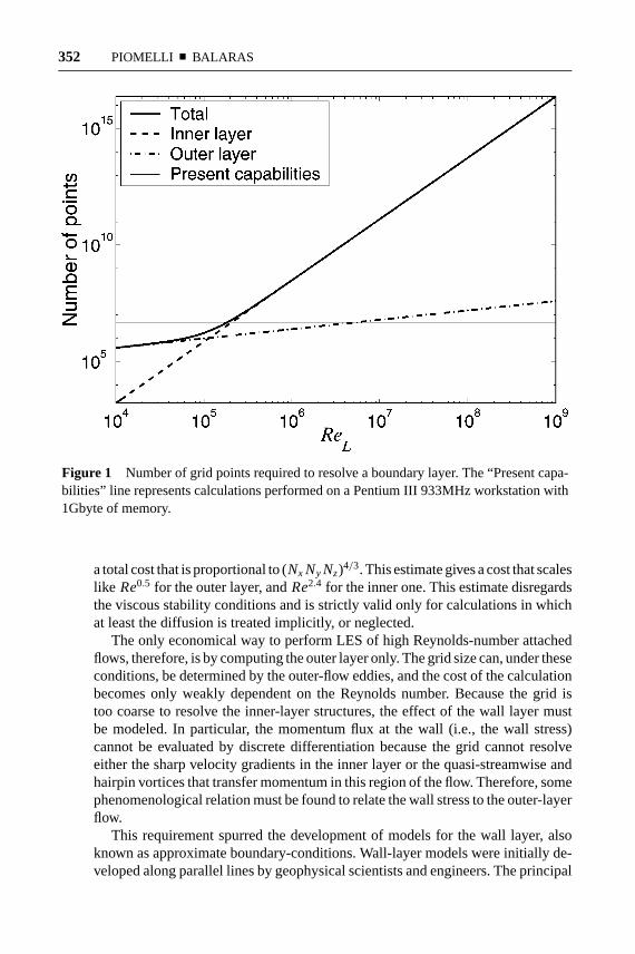
Using the estimates for boundary-layer flows, Figure 1 shows that atReL =o(106), 99% of the points are used to resolve an inner layer whose thickness isonly 10% of the boundary layer. As a consequence, the number of points requiredby LES if the inner layer is resolved exceeds present computational capabilitiesalready at moderate Reynolds numbers.

To estimate the cost of the calculation, one must consider that the equations ofmotion must be integrated for a time proportional to the integral timescale of theflow, with a time step limited by the need to resolve the life of the smallest eddy.Reynolds (1990) estimates the cost by assuming that the operation count scaleslike the number of points and that the time step be determined by the timescale ofthe smallest eddy, which is inversely proportional to its length scale and, therefore,to the grid size. This gives a number of time steps proportional to (Nx NyNz)1/3 and



Figure 1 Number of grid points required to resolve a boundary layer. The “Present capa-bilities” line represents calculations performed on a Pentium III 933MHz workstation with1Gbyte of memory.

a total cost that is proportional to (Nx NyNz)4/3. This estimate gives a cost that scaleslike Re0.5 for the outer layer, andRe2.4 for the inner one. This estimate disregardsthe viscous stability conditions and is strictly valid only for calculations in whichat least the diffusion is treated implicitly, or neglected.

The only economical way to perform LES of high Reynolds-number attachedflows, therefore, is by computing the outer layer only. The grid size can, under theseconditions, be determined by the outer-flow eddies, and the cost of the calculationbecomes only weakly dependent on the Reynolds number. Because the grid istoo coarse to resolve the inner-layer structures, the effect of the wall layer mustbe modeled. In particular, the momentum flux at the wall (i.e., the wall stress)cannot be evaluated by discrete differentiation because the grid cannot resolveeither the sharp velocity gradients in the inner layer or the quasi-streamwise andhairpin vortices that transfer momentum in this region of the flow. Therefore, somephenomenological relation must be found to relate the wall stress to the outer-layerflow.

This requirement spurred the development of models for the wall layer, alsoknown as approximate boundary-conditions. Wall-layer models were initially de-veloped along parallel lines by geophysical scientists and engineers. The principal

30 Nov 2001 9:53 AR AR151-14.tex AR151-14.SGM LaTeX2e(2001/05/10)P1: GJC


difference between the two fields is the presence of stratification, which is impor-tant in meteorological flows but usually not in engineering. Stratification effectsare not treated in the present review, which concentrates on the engineering appli-cations and development and only briefly outlines the models used by geophysicalscientists and meteorologists.

In the following, first the basic philosophy of wall-layer modeling is laid out, andthe assumptions and approximations common to most of the methods proposedin the literature are discussed. Then, in Sections 2.1–3, a review of the variousapproaches that have appeared in the literature is carried out. This is followed bya discussion of other sources of errors that may appear in calculations in whichonly the outer layer is computed. Some conclusions are drawn in Section 4.

2. WALL-LAYER MODELING

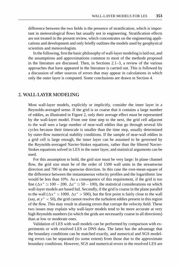
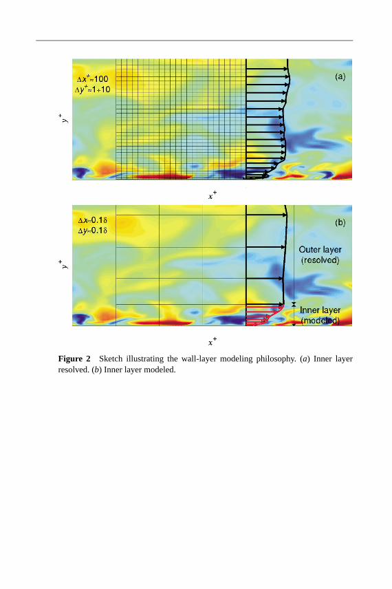
Most wall-layer models, explicitly or implicitly, consider the inner layer in aReynolds-averaged sense. If the grid is so coarse that it contains a large numberof eddies, as illustrated in Figure 2, only their average effect must be representedby the wall-layer model. From one time step to the next, the grid cell adjacentto the wall sees a large number of near-wall eddies that go through several lifecycles because their timescale is smaller than the time step, usually determinedby outer-flow numerical stability conditions. If the sample of near-wall eddies ina grid cell is large enough, the inner layer can be assumed to be governed bythe Reynolds-averaged Navier-Stokes equations, rather than the filtered Navier-Stokes equations solved in LES in the outer layer, and statistical arguments can beused.

For this assumption to hold, the grid size must be very large: In plane channelflow, the grid size must be of the order of 1500 wall units in the streamwisedirection and 700 in the spanwise direction. In this case the root-mean-square ofthe difference between the instantaneous velocity profiles and the logarithmic lawwould be less than 10%. As a consequence of this requirement, if the grid is toofine (1x+ ' 100− 200,1z+ ' 50− 100), the statistical considerations on whichwall-layer models are based fail. Secondly, if the grid is coarse in the plane parallelto the wall (1x+> 1000,1z+> 500), but the first point is fairly close to the wall(say, aty+< 50), the grid cannot resolve the turbulent eddies present in this regionof the flow. This may result in aliasing errors that corrupt the velocity field. Thesetwo issues may explain why wall-layer models tend to be more accurate at veryhigh Reynolds numbers (in which the grids are necessarily coarse in all directions)than at low or moderate ones.

Validation of LES with wall models can be performed by comparison with ex-periments or with resolved LES or DNS data. The latter has the advantage thatthe boundary conditions can be matched exactly, and numerical and SGS model-ing errors can be separated (to some extent) from those due to the approximateboundary conditions. However, SGS and numerical errors in the resolved LES are



usually largest in the near-wall layer; thus it is conceivable that calculations thatuse “perfect” wall-layer models could give more accurate predictions than resolvedones. Furthermore, the Reynolds number achievable by resolved LES and DNS,as mentioned above, is quite low; this can affect the accuracy of the wall models.High Reynolds-number experimental data is more easily available, but it is moredifficult to reproduce the experimental setup accurately, and differences betweencalculations and experimental data are often due to differences in the boundaryconditions (see, for example, the discussion in Kaltenbach et al. 1999) as well asto numerical and modeling errors.

The simplest approach to relate the wall stress to the outer velocity is to neglectall terms in the streamwise momentum equation except the Reynolds-stress gradi-ent. This implies that the acceleration and pressure gradient at the first grid pointare negligible and that the first grid point is far enough from the wall that viscouseffects are negligible. If, in addition, the shear stress is assumed to be constantbetween the wall and the first point, one can derive a logarithmic velocity profilein the inner layer either of the form

u+ = u

uτ= 1

κlog y+ + B, (3)

whereκ is the von Karman constant, or

u+ = 1

κlog

y

yo, (4)

whereyo is the roughness height. This profile can be used to obtain the wall stressgiven the velocity (obtained from the outer-flow calculation) at the first grid point.The details of this approach are discussed in Section 2.1.

More recently, zonal approaches in which the RANS equations are solved inthe inner layer have been proposed and tested to remove those limiting assump-tions. They are described in Section 2.2. Other methods are discussed in the finalsubsection.

2.1. Equilibrium Laws

The limitations of LES, when applied to wall-bounded flows, were recognized inthe very early stages of the development of the technique: In the ground-breakingLES of plane channels and annuli by Deardorff (1970) and Schumann (1975),respectively, approximate wall-boundary conditions were introduced to model theeffect of the wall layer, which could not be resolved with the computer poweravailable at that time even at moderate Reynolds numbers. In the methodologythey proposed, information from the outer flow is used to determine the local wallstress, which is then fed back to the outer LES in the form of the proper momentumflux at the wall due to normal diffusion. The no-transpiration condition was used onthe wall-normal velocity component. Today this general approach is still in use invarious forms. The cost of these calculations is due to the outer-layer computationonly and is proportional toRe0.5 for spatially developing flows.



Deardorff (1970), in his channel flow computations, restricted the second deriva-tives of the velocity at the first off-wall grid point to be

∂2u

∂y2= − 1

κY2+ ∂

2u

∂z2, (5)

∂2w

∂y2= ∂2w

∂x2, (6)

wherex indicates the streamwise direction,zthe spanwise direction, andy the wall-normal direction;u, v, andw are the velocity components in the three coordinatedirections, respectively, and an overbar denotes a filtered (or large-scale) quantity.Y is the location of the first point away from the wall. Equation 5 forces the plane-averaged velocity profile to satisfy a logarithmic law in the mean at pointY. Allquantities in Equations 5 and 6 are normalized byuτ andv.

The results obtained by Deardorff (1970) for the turbulent channel flow atinfinite Reynolds number do not compare well with the experimental data of Laufer(1950). The wall model, however, most likely has a small contribution to theseerrors, which are mainly due to the resolution in the outer layer that was notsufficient to resolve the large energy-carrying structures. A total of 6720 gridnodes were used, which corresponds to approximately 400 points to resolve avolumeδ3; this is six times less than the number of required points estimated byChapman (1979). When using an alternative set of boundary conditions proposedin the same paper, which essentially implies that the logarithmic law (Equation 4)holds locally, no difference was observed in the statistics.

Schumann (1975) used conditions that directly relate the shear stresses at thewall, τxy,w andτyz,w, to the velocity in the core by

τxy,w(x, z) = 〈τw〉〈u(x,Y, z)〉 u(x,Y, z), (7)

τyz,w(x, z) = ν w(x,Y, z)

Y, (8)

where〈·〉 denotes averaging over a plane parallel to the solid wall. The meanstress〈τw〉 is assigned a value equal to the given pressure gradient, or it canbe calculated iteratively using Newton iterations and requiring that the plane-averaged velocity at the first grid point,〈u(x,Y, z)〉, satisfy the logarithmic law(Equation 4) at pointY. In phase with the adjacent local outer velocity, the resultantstreamwise component (τxy) of local wall-stress fluctuates around the mean value.The spanwise component (τyz) is obtained by assuming a linear velocity profileand a constant-eddy viscosity in the grid cell adjacent to the wall. The channel-flow computations carried out in this study gave results in very good agreementwith the reference experimental data. Given the poor agreement with experimentsin Deardorff’s (1970) simulations (discussed above) this series of computationswas essentially the first to demonstrate the feasibility of LES using approximate



wall-boundary conditions. In a later study Grötzbach (1987) used a similar ap-proach to assign the wall-heat flux in calculations of turbulent flows with heattransfer and obtained favorable results.

Piomelli et al. (1989) applied conditions similar to Equations 7 and 8. However,to take into account the inclination of the elongated structures in the near-wallregion, they required that the wall stress be correlated to the instantaneous velocitysome distance downstream of the point where the wall stress is required:

τxy,w = 〈τw〉〈u(x,Y, z)〉 u(x +1s,Y, z), (9)

τyz,w = 〈τw〉〈u(x,Y, z)〉 w(x +1s,Y, z), (10)

where1s is a streamwise displacement; its optimum value can be obtained fromDNS or experimental data and is approximately1s = Y cot 8◦ for 30< Y+ < 50,and1s = Y cot 13◦ for larger distances for the range of Reynolds numbers investi-gated. The plane-averaged wall stress is obtained by iterative solution of Equation 3as in the Schumann (1975) model above. These changes yielded improved resultswith respect to the original formulation and were used by Balaras et al. (1995)to study the flow in a plane channel for a range of Reynolds numbers in con-junction with the dynamic SGS model, with results in excellent agreement withexperimental and DNS data.

All the above approximate boundary conditions are applicable to geometricallysimple flows in which the mean wall stress can be obtained from some form ofthe law-of-the-wall. Extension to more complex configurations is possible onlyif the mean wall stress can be specified. Wu & Squires (1998) performed LESof a three-dimensional boundary layer over a swept bump using an approachsimilar to that of Schumann (1975): Equations 7 and 8 were used, with the meanwall stress obtained from a separate RANS calculation. The mean velocity inthese equations was computed by performing spanwise averages at each timestep during the calculation. Their results are in fairly good agreement with thereference experimental data. This type of approach could be useful in some cases inwhich RANS simulations or prior experimental studies could provide a reasonableestimate of the mean wall stress, but extension to complex flows is impracticalbecause it relies on the accuracy of the RANS approach.

Most of the models described above imply that the logarithmic law-of-the-wallholds in the mean: Deardorff (1970) enforced this through the second derivativeof the velocity (Equation 5); Schumann (1975) and Piomelli et al. (1989) did soby calculating the mean wall stress from the iterative solution of Equation 3 foruτ , given u at the first grid point off the wall. Alternatively, the logarithmic lawcan be enforced locally and instantaneously, and the wall stress can be computedby assuming that it is aligned with the outer horizontal velocity, as suggested byDeardorff (1970). This method was extensively tested in a study by Mason &Callen (1986) and is based on local equilibrium of the near-wall region; its validity



strongly depends on the size of the averaging volume (the grid cell), which mustcontain (as mentioned earlier) a significant sample of inner-layer eddies. In a similarmanner Werner & Wengle (1993) fit the local horizontal velocity to a power lawmatched to a linear profile near the wall to compute the local stress. The resultsin both cases are not very different from the ones with the other models discussedabove.

Although a discussion of the important issues in geophysical calculations isbeyond the scope of this paper, it should be mentioned that most wall-layer modelsused in meteorology are of this type. Moeng (1984), for instance, also computesuτ by imposing an instantaneous logarithmic law at the first grid point, with acorrection for the wall heat flux. A similar relationship is used to evaluate thetemperature gradient at the wall (see, for instance, Zhang et al. 1996).

Hoffmann & Benocci (1995) derived an analytical expression for the local stressby integrating analytically the boundary-layer equations coupled with an algebraicturbulence model:

vY = − d

dx

∫ Y

0u dy (11)

τxy,w =[νtot∂u

∂y

]Y

− uYvY + d

dx

∫ Y

0u2 dy

−Yd Pe

dx− d

dt

∫ Y

0u dy, (12)

whereνtot is the total eddy viscosity (sum of molecular and SGS) anddPe/dx is theexternal pressure gradient. Hoffman & Benocci (1995) argued that the sum of thetwo advective terms (the second and third on the right-hand side of Equation 12)can be neglected (they point out that it is not legitimate to neglect only one of them,only their difference). They approximated the unsteady term using a discretizedtime derivative and order-of-magnitude arguments and modeled the viscous diffu-sion usingκy as the length scale in a mixing-length model. Then, the calculationof the wall stress required only the velocityuY. The results for a channel flow and arotating channel flow are in good agreement with resolved LES and experimentalstudies.

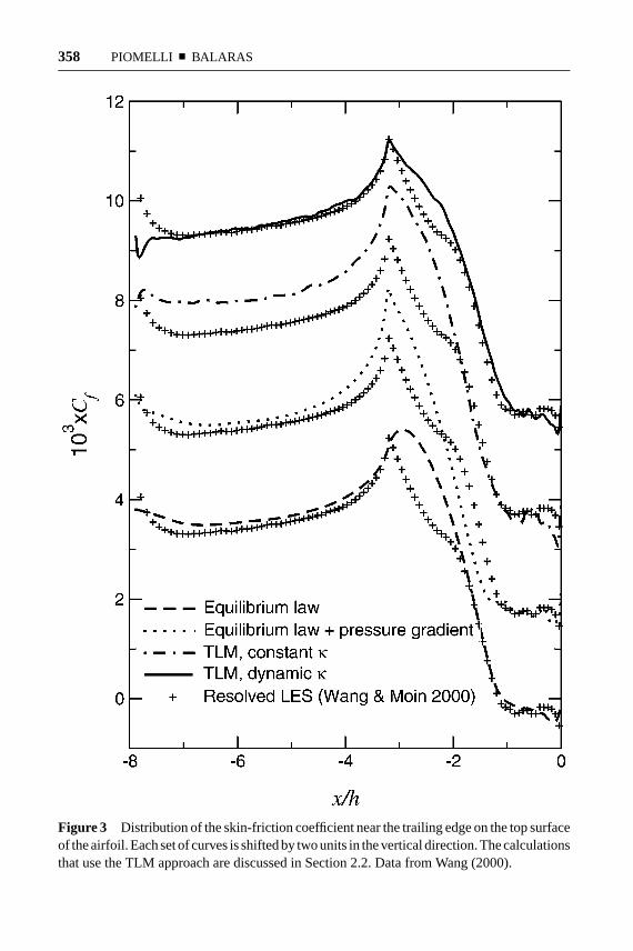
The same approach was used by Wang (1999) to calculate the flow over thetrailing edge of an airfoil. He examined two cases, one in which only the vis-cous and turbulent diffusion were used in the equation and one in which thepressure gradient was included. The unsteady term was always neglected. Theapproximate–boundary condition calculation was in good agreement with the re-solved one (Wang & Moin 2000) in the zero or favorable pressure-gradient region(see Figure 3), but the flow in the adverse pressure-gradient region was not pre-dicted accurately. Immediately downstream of the sharp peak in the skin-frictioncoefficient in Figure 3, the wall model does not respond correctly to the transi-tion from the favorable to the adverse pressure gradient. The frequency spectra of



Figure 3 Distribution of the skin-friction coefficient near the trailing edge on the top surfaceof the airfoil. Each set of curves is shifted by two units in the vertical direction. The calculationsthat use the TLM approach are discussed in Section 2.2. Data from Wang (2000).



wall-pressure fluctuations agree well with those obtained from the resolved calcu-lation, except in the adverse pressure-gradient and separated regions. Wang (1999)also computed the far-field noise generated by the sharp trailing edge and found thatthe predictions of the calculations with approximate boundary conditions did notmatch the resolved ones in the frequency range associated with scales generated inthe separation region, whereas at other frequencies the agreement was acceptable.

2.2. Zonal Approaches

Zonal approaches are based on the explicit solution of a different set of equationsin the inner layer. There are two approaches: In one, known as the Two-LayerModel (TLM), two separate grids are used. In the other, which is based on theDetached Eddy Simulation method proposed by Spalart et al. (1997), a single gridis used, and only the turbulence model changes.

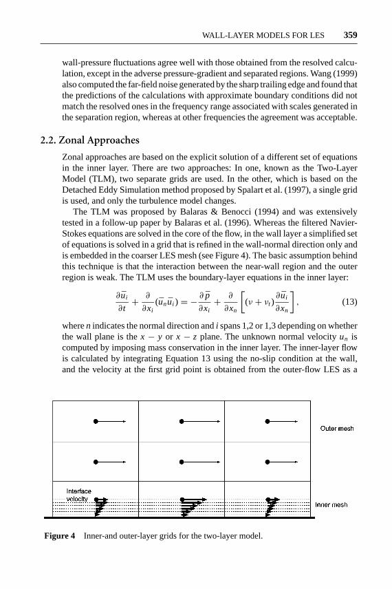
The TLM was proposed by Balaras & Benocci (1994) and was extensivelytested in a follow-up paper by Balaras et al. (1996). Whereas the filtered Navier-Stokes equations are solved in the core of the flow, in the wall layer a simplified setof equations is solved in a grid that is refined in the wall-normal direction only andis embedded in the coarser LES mesh (see Figure 4). The basic assumption behindthis technique is that the interaction between the near-wall region and the outerregion is weak. The TLM uses the boundary-layer equations in the inner layer:

∂ui

∂t+ ∂

∂xi(unui ) = − ∂ p

∂xi+ ∂

∂xn

[(ν + νt )

∂ui

∂xn

], (13)

wheren indicates the normal direction andi spans 1,2 or 1,3 depending on whetherthe wall plane is thex − y or x − z plane. The unknown normal velocityun iscomputed by imposing mass conservation in the inner layer. The inner-layer flowis calculated by integrating Equation 13 using the no-slip condition at the wall,and the velocity at the first grid point is obtained from the outer-flow LES as a

Figure 4 Inner-and outer-layer grids for the two-layer model.



“freestream” condition. The wall-stress components obtained from the integrationof Equation 13 in the inner layer are then used as boundary conditions for theouter-flow calculation.

The cost of this method is marginally higher than the cost of calculations thatuse equilibrium boundary-conditions because the inner layer requires a small per-centage of the total cost of the calculation. Two one-dimensional problems aresolved, and no Poisson-equation inversion is required to obtain the pressure.

In Balaras & Benocci (1994) and Balaras et al. (1996) an algebraic eddy vis-cosity model was used to parameterize all scales of motion in the wall layer:

νt = (κy)2D(y)∣∣S∣∣ , (14)

wherey is the distance from the wall,∣∣S∣∣ is the magnitude of the resolved strain-

rate tensor, andD(y) is a damping function that assures the correct behavior ofνt

at the wall:

D(y) = 1− exp[−(y+/A+)3], (15)

whereA+ = 25.Balaras et al. (1996) applied the TLM to channel flow for Reynolds numbers

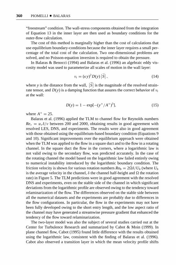
Reτ = uτ δ/ν between 200 and 2000, obtaining results in good agreement withresolved LES, DNS, and experiments. The results were also in good agreementwith those obtained using the equilibrium-based boundary condition (Equations 9and 10). Significant improvements over the equilibrium approach were obtainedwhen the TLM was applied to the flow in a square duct and to the flow in a rotatingchannel. In the square duct the flow in the corners, where a logarithmic law isnot valid owing to the secondary flow, was predicted accurately. In the case ofthe rotating channel the model based on the logarithmic law failed entirely owingto numerical instability introduced by the logarithmic boundary condition. Thefriction velocity is shown for various rotation numbersRob = 2Äδ/Ub (whereUb

is the average velocity in the channel,δ the channel half-height andÄ the rotationrate) in Figure 5. The TLM predictions were in good agreement with the resolvedDNS and experiments, even on the stable side of the channel in which significantdeviations from the logarithmic profile are observed owing to the tendency towardrelaminarization of the flow. The differences observed on the stable side betweenall the numerical datasets and the experiments are probably due to differences inthe flow configurations. In particular, the flow in the experiments may not havebeen fully developed owing to the short entry length, and the low aspect ratio ofthe channel may have generated a streamwise pressure gradient that enhanced thetendency of the flow toward relaminarization.

The two-layer model was also the subject of several studies carried out at theCenter for Turbulence Research and summarized by Cabot & Moin (1999). Inplane channel flow, Cabot (1995) found little difference with the results obtainedusing the logarithmic law, consistent with the finding of Balaras et al. (1996).Cabot also observed a transition layer in which the mean velocity profile shifts



Figure 5 Friction velocity in rotating channel flow.•, Experiments (Johnston et al. 1972);---, —·—, best fit to experimental data (Johnston et al. 1972);+, DNS (Kristoffersen &Andersson 1993);¥, DNS (Lamballais et al. 1998);¤ resolved LES (Lamballais et al. 1998);×, resolved LES (Piomelli & Liu 1995);M, LES with wall models (Balaras et al. 1996).

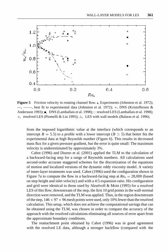
from the imposed logarithmic value at the interface (which corresponds to aninterceptB = 5.5) to a profile with a lower intercept (B ' 5) that better fits theexperimental data at high Reynolds number (Figure 6). This results in decreasedmass flux for a given pressure gradient, but the error is quite small: The maximumvelocity is underestimated by approximately 3%.

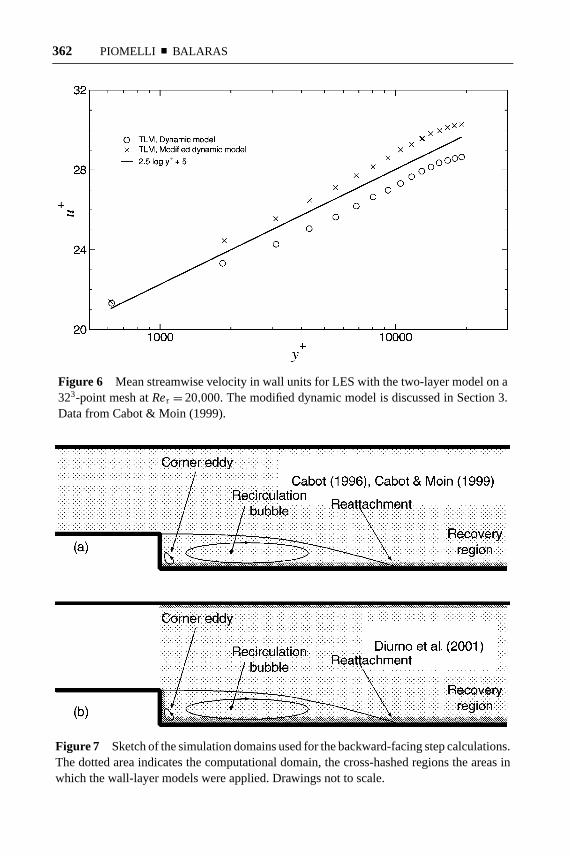
Cabot (1996) and Diurno et al. (2001) applied the TLM to the calculation ofa backward-facing step for a range of Reynolds numbers. All calculations usedsecond-order accurate staggered schemes for the discretization of the equationsof motion and localized versions of the dynamic eddy viscosity model. A varietyof inner-layer treatments was used. Cabot (1996) used the configuration shown inFigure 7a to compute the flow in a backward-facing step atReh = 28,000 (basedon step height and inlet velocity) and with a 4:5 expansion ratio. His configurationand grid were identical to those used by Akselvoll & Moin (1995) for a resolvedLES of this flow; downstream of the step, the first 10 grid points in the wall-normaldirection were removed, and the TLM was applied. Thus, in the region downstreamof the step, 146× 97× 96 mesh points were used, only 10% fewer than the resolvedcalculation. This setup, which does not achieve the computational savings that canbe obtained using the TLM, was chosen in order to compare the accuracy of theapproach with the resolved calculations eliminating all sources of error apart fromthe approximate boundary conditions.

The reattachment point obtained by Cabot (1996) was in good agreementwith the resolved LE data, although a stronger backflow (compared with the



Figure 6 Mean streamwise velocity in wall units for LES with the two-layer model on a323-point mesh atReτ = 20,000. The modified dynamic model is discussed in Section 3.Data from Cabot & Moin (1999).

Figure 7 Sketch of the simulation domains used for the backward-facing step calculations.The dotted area indicates the computational domain, the cross-hashed regions the areas inwhich the wall-layer models were applied. Drawings not to scale.



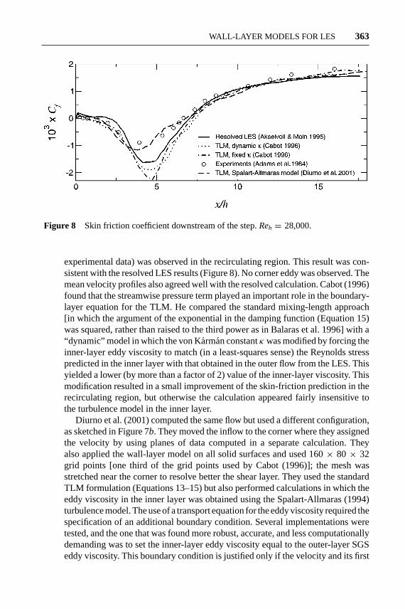
Figure 8 Skin friction coefficient downstream of the step.Reh = 28,000.

experimental data) was observed in the recirculating region. This result was con-sistent with the resolved LES results (Figure 8). No corner eddy was observed. Themean velocity profiles also agreed well with the resolved calculation. Cabot (1996)found that the streamwise pressure term played an important role in the boundary-layer equation for the TLM. He compared the standard mixing-length approach[in which the argument of the exponential in the damping function (Equation 15)was squared, rather than raised to the third power as in Balaras et al. 1996] with a“dynamic” model in which the von Kárman constantκ was modified by forcing theinner-layer eddy viscosity to match (in a least-squares sense) the Reynolds stresspredicted in the inner layer with that obtained in the outer flow from the LES. Thisyielded a lower (by more than a factor of 2) value of the inner-layer viscosity. Thismodification resulted in a small improvement of the skin-friction prediction in therecirculating region, but otherwise the calculation appeared fairly insensitive tothe turbulence model in the inner layer.

Diurno et al. (2001) computed the same flow but used a different configuration,as sketched in Figure 7b. They moved the inflow to the corner where they assignedthe velocity by using planes of data computed in a separate calculation. Theyalso applied the wall-layer model on all solid surfaces and used 160× 80× 32grid points [one third of the grid points used by Cabot (1996)]; the mesh wasstretched near the corner to resolve better the shear layer. They used the standardTLM formulation (Equations 13–15) but also performed calculations in which theeddy viscosity in the inner layer was obtained using the Spalart-Allmaras (1994)turbulence model. The use of a transport equation for the eddy viscosity required thespecification of an additional boundary condition. Several implementations weretested, and the one that was found more robust, accurate, and less computationallydemanding was to set the inner-layer eddy viscosity equal to the outer-layer SGSeddy viscosity. This boundary condition is justified only if the velocity and its first



derivative are smooth at the interface, which in all computations was true at leastin the mean.

Diurno et al. (2001) obtained quite good agreement with the experiments(Figure 8), both with the Spalart-Allmaras (1994) model and with the standardalgebraic eddy-viscosity model in the inner layer. They found that the flow fieldwas quite insensitive to the inner-layer treatment, consistent with the results byCabot (1996). They did observe a secondary recirculating region and a cornereddy that was, however, excessively elongated in the wall-normal direction. Sev-eral factors can explain the difference between these results and those obtainedby Cabot (1996) using a similar model and numerical scheme. First is the dif-ference in the configuration: Akselvoll & Moin (1995) and Cabot (1996) had adevelopment region upstream of the step in which the grid resolution may not havebeen sufficient to resolve the boundary layer properly. The wall stress predictedby the LES throughout this region is, in fact, 30% lower than in the experiments.Diurno et al. (2001), on the other hand, had no development region but assigned aboundary layer obtained from a separate calculation that matched the experimentalwall stress. Because the state of the boundary layer at the separation point is veryimportant in determining the flow dynamics, this difference can have significanteffects. Second, the mesh used by Diurno et al. (2001) near the corner was finer inthe streamwise and wall-normal directions compared to that employed by Cabot(1996). Notice that, although Cabot (1996) employed 96 points in this direction, heresolved the wall layer on the upper wall, which was modeled in the computationsby Diurno et al. (2001).

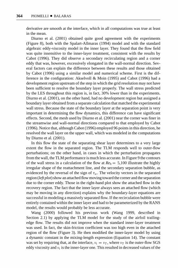
In this flow the state of the separating shear layer determines to a very largeextent the flow in the separated region. The TLM responds well to outer-flowperturbations; on the other hand, in cases in which the perturbation propagatesfrom the wall, the TLM performance is much less accurate. In Figure 9 the contoursof the wall stress in a calculation of the flow atReh= 5,100 illustrate the highlyirregular shape of the reattachment line, and the secondary separation bubble, asevidenced by the reversal of the sign ofτw. The velocity vectors in the separatedregion (left plot) show an attached flow moving toward the corner and the separationdue to the corner eddy. Those in the right-hand plot show the attached flow in therecovery region. The fact that the inner layer always sees an attached flow (whichmay be moving in any direction) explains why the boundary-layer equations aresuccessful in modeling a massively separated flow. If the recirculation bubble wereentirely contained within the inner layer and had to be parameterized by the RANSmodel, the results would probably be less accurate.

Wang (2000) followed his previous work (Wang 1999, described inSection 2.1) by applying the TLM model for the study of the airfoil trailing-edge flow. The results did not improve when the standard inner-layer treatmentwas used. In fact, the skin-friction coefficient was too high even in the attachedregion of the flow (Figure 3). He then modified the inner-layer model by usinga dynamic constant in the mixing-length expression (Equation 14). The constantwas set by requiring that, at the interface,νt = νT , whereνT is the outer-flow SGSeddy viscosity andνt is the inner-layer one. This resulted in decreased values of the



Figure 9 Contours of the instantaneous wall-stress downstream of the step and instanta-neous velocity vectors in thexy−plane at two locations. The scaling of the vectors on theleft-hand-side figure is magnified by a factor of three compared with the right-hand-side. Theinterface is shown by a thick line and the contour interval is1τw = 2× 10−4. Dotted contoursare negative.Reh = 5,100. From Diurno et al. (2001).

inner-layer eddy viscosity (lower by a factor of approximately 3) and in improvedagreement with the resolved LES (Figure 3), especially in the adverse pressure-gradient and separated regions. The velocity spectra and the far-field noise werealso in better agreement with the resolved case.

Another approach to wall-layer modeling is the Detached Eddy Simulation(DES), introduced by Spalart et al. (1997) as a method to compute massivelyseparated flows. DES is a hybrid approach that combines the solution of the RANSequations in the attached boundary layers with LES in the separated regions inwhich the detached eddies are important. Recent reviews of the DES formulationand achievements can be found in Spalart (2000) and Strelets (2001). AlthoughDES is not a zonal approach, as it uses a single grid, the turbulence model usedseparates a RANS region from an LES one, effectively creating two zones, onein which the RANS model has control over the solution and another in which theresolved eddies govern the flow. Notice that, because no zonal interface exists,the velocity field is smooth everywhere. Its original formulation used the Spalart-Allmaras (1994) model, a one-equation model in which a transport equation for theeddy viscosity is solved. By modifying the model length scale to account for thefine resolution in the LES regions, the production of eddy viscosity is decreasedfar from solid surfaces. When production and destruction are equal, the model



behavior is similar to that of a Smagorinsky (1963) eddy-viscosity model (Strelets2001). Because the grid size in the plane parallel to the walls scales with the outer-flow eddies, although the first grid point must be aty+ ' 1 to ensure accuratecalculation of the wall stress by the finite-difference method, the cost of this methodcompared to a resolved calculation is a weaker function of the Reynolds number.Nikitin et al. (2000) estimate the cost to be proportional toReτ , which correspondsroughly toRe0.9

L .In the standard DES approach the entire boundary layer is modeled by RANS.

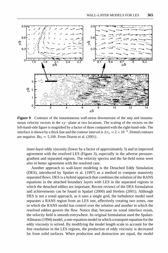
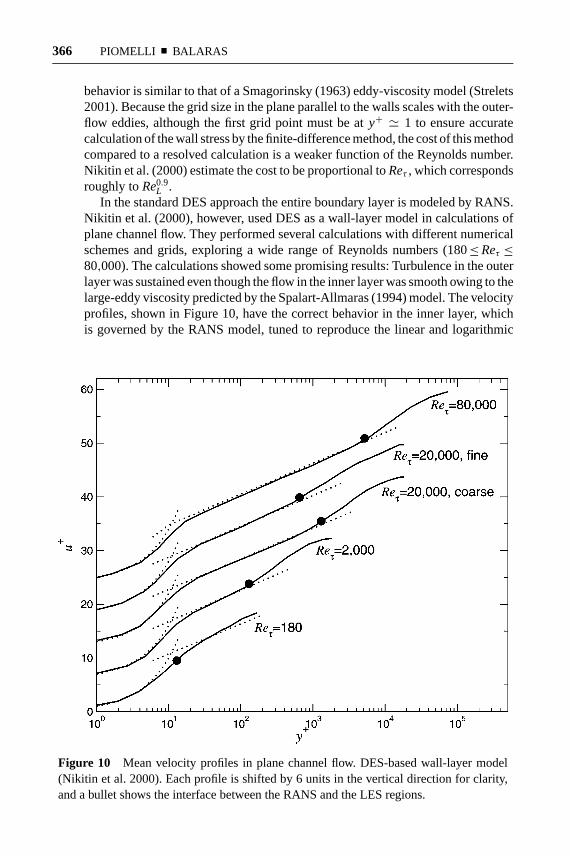
Nikitin et al. (2000), however, used DES as a wall-layer model in calculations ofplane channel flow. They performed several calculations with different numericalschemes and grids, exploring a wide range of Reynolds numbers (180≤Reτ ≤80,000). The calculations showed some promising results: Turbulence in the outerlayer was sustained even though the flow in the inner layer was smooth owing to thelarge-eddy viscosity predicted by the Spalart-Allmaras (1994) model. The velocityprofiles, shown in Figure 10, have the correct behavior in the inner layer, whichis governed by the RANS model, tuned to reproduce the linear and logarithmic

Figure 10 Mean velocity profiles in plane channel flow. DES-based wall-layer model(Nikitin et al. 2000). Each profile is shifted by 6 units in the vertical direction for clarity,and a bullet shows the interface between the RANS and the LES regions.

30 Nov 2001 9:55 AR AR151-14.tex AR151-14.SGM LaTeX2e(2001/05/10)P1: GJC


profiles in flows of this kind. As the flow transitions into the LES region, however,an unphysical “DES buffer layer” is formed in which the velocity gradient is toohigh. This buffer layer becomes what appears to be an extended wake region,but is instead a logarithmic layer with a high intercept and, in some cases, anincorrect slope. The high intercept is particularly clear in the fine calculation atReτ = 20,000, in which it extends roughly between 3000< y+< 15,000. Whenthe resolution in the outer LES region was insufficient (1x = 1z = 0.1δ), theslope of this spurious logarithmic region was also incorrect. Only at the lowestReynolds number, in which the grid was fine enough to perform a coarse DNS,were accurate results obtained in the outer layer. These errors were reflected inthe skin-friction coefficient, which was underpredicted by approximately 15% inmost of the calculations. Although the outer-layer resolution could affect the slopeof the logarithmic layer in the LES region, the high intercept must be attributedto other causes because refining the grid in theReτ = 20,000 calculation did notresult in significant improvements.

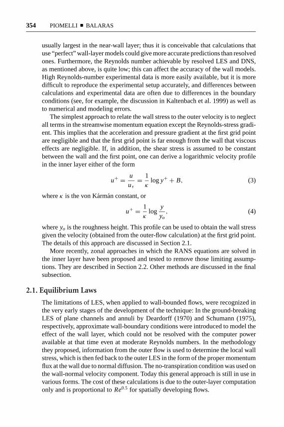
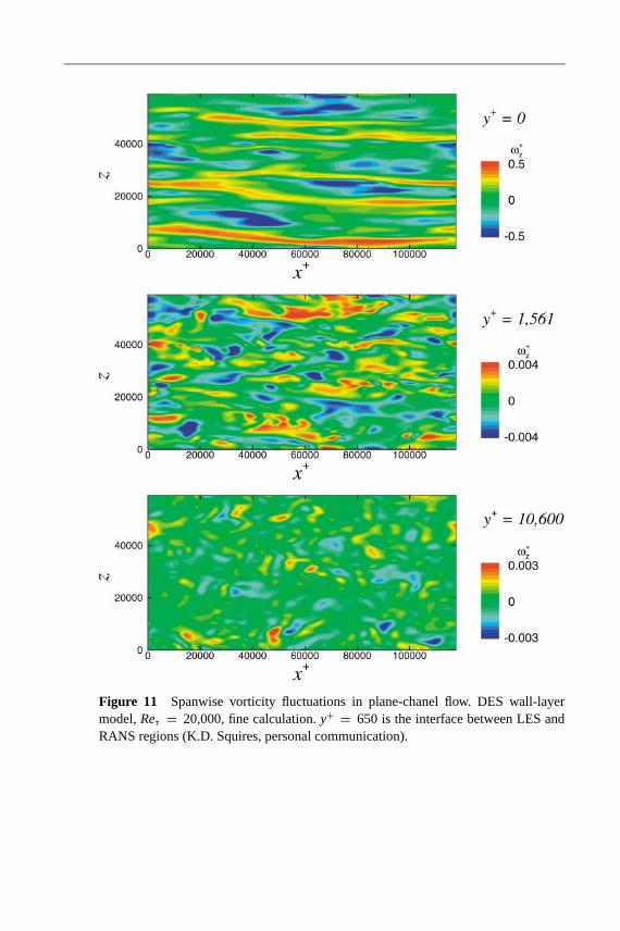
Because the inner layer was smooth, unphysical, nearly one-dimensional, wallstreaks were present in the RANS region, shown in Figure 11, and shorter-scaleouter-layer eddies were progressively formed as one moved away from the wall.Baggett (1998) argues that the presence of these artificial streaks causes a de-correlation betweenu andv fluctuations that must be compensated by a highervelocity gradient to balance streamwise momentum, which shifts the intercept ofthe LES logarithmic region to a higher value. The mechanism of generation ofthese artificial streaks is not fully understood. In particular, it is not clear whetherthey are generated by the nonlinear response of the inner-layer model to outer-flowperturbations or whether the inner layer is forcing the outer flow to have incorrectlength scales, thereby causing this transition layer to exist.

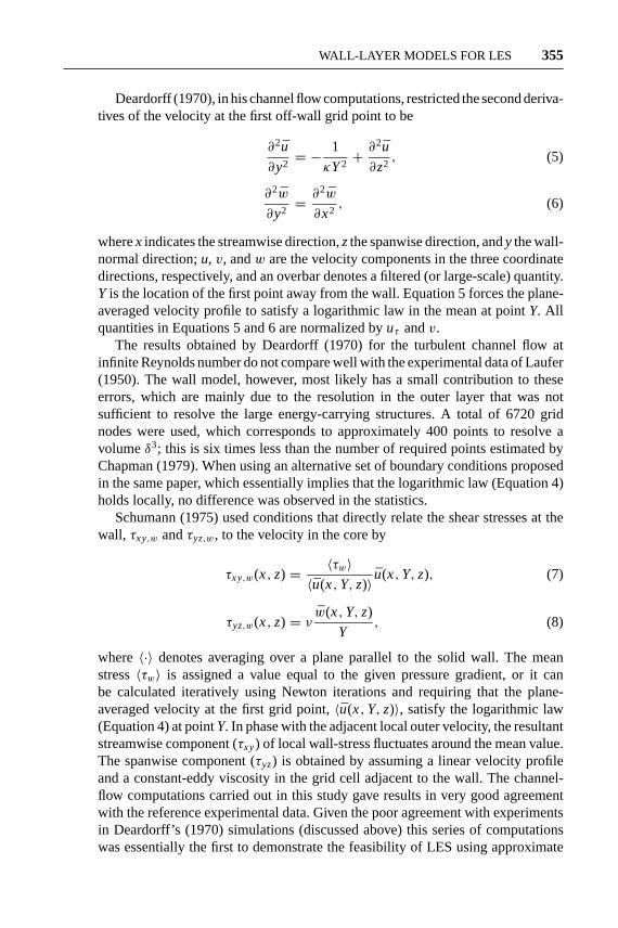
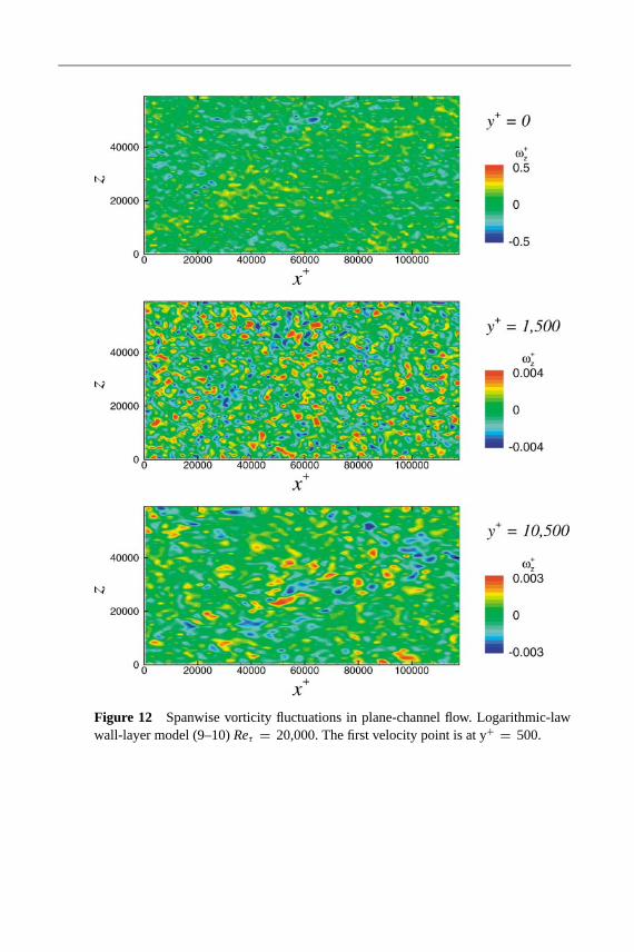
In models based on the logarithmic law different results can be observed.Figure 12 shows contours of the vorticity in a channel-flow calculation carriedout in a similar configuration (in terms of domain size, grid in the streamwise andspanwise directions) to that used in the DES case. The outer-layer eddies in thiscase leave a much stronger footprint on the inner layer, which has the same lengthscales as the outer layer.

2.3. Other Methods

In the methodologies discussed in Sections 2.1 and 2.2 the local wall stress requiredto impose boundary conditions to the outer LES is computed either from someform of law-of-the-wall or by solving numerically a set of simplified equations.Alternative methods have also been explored over the past years. Bagwell et al.(1993) developed an approach that attempts to incorporate more knowledge ofwall-layer coherent structures into wall models. They used the linear stochasticestimate (LSE) approach (Adrian 1979) to obtain the local wall-shear stress giventhe outer flow. LSE provides the best linear estimate (in the least-squares sense)of the velocity field corresponding to a given “event” (the velocity, strain rate,or pressure at one or more points in the field). Bagwell et al. (1993) assigned an



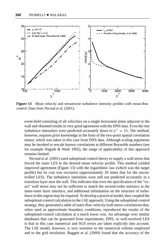
Figure 13 Mean velocity and streamwise turbulence intensity profiles with mean-flowcontrol. Data from Nicoud et al. (2001).

event-field consisting of all velocities on a single horizontal plane adjacent to thewall and obtained results in very good agreement with the DNS data. Even the rmsturbulence intensities were predicted accurately down toy+ = 15. The method,however, requires prior knowledge in the form of the two-point spatial correlationtensor, which was taken in this case from DNS data. Although scaling argumentsmay be invoked to rescale known correlations at different Reynolds numbers (seefor example Naguib & Wark 1992), the range of applicability of this approachremains limited.

Nicoud et al. (2001) used suboptimal control theory to supply a wall stress thatforced the outer LES to the desired mean velocity profile. This method yieldedimproved agreement (Figure 13) with the logarithmic law (which was the targetprofile) but its cost was excessive (approximately 20 times that for the uncon-trolled LES). The turbulence intensities were still not predicted accurately in atransition layer near the wall. This indicates that even the specification of the “ex-act” wall stress may not be sufficient to match the second-order statistics at theinner-outer layer interface, and additional information on the structure of turbu-lence in this region may be required. To develop a practical model, they coupled thesuboptimal-control calculation to the LSE approach. Using the suboptimal-controlstrategy, they generated a table of outer-flow velocity/wall-stress correlations that,when used as approximate boundary conditions, reproduced the results of thesuboptimal-control calculation at a much lower cost. An advantage over similardatabases that can be generated from experiments, DNS, or well-resolved LESis that in this case numerical and SGS errors are taken explicitly into account.The LSE model, however, is very sensitive to the numerical scheme employedand to the grid resolution. Baggett et al. (2000) found that the accuracy of the



LSE model deteriorates significantly when the grid is modified or when a differ-ent numerical scheme is used than the one employed in the suboptimal-controlcalculation.

3. OTHER SOURCES OF ERROR

Near the wall, in the outer layer, the dominant eddies become comparable tothe grid size, violating the assumptions on which most SGS stress models arebased. Furthermore, the accurate evaluation of the strain-rate tensor, which isrequired by most eddy-viscosity SGS models, may be inaccurate. Finally, theexplicit filtering operations commonly used to perform a dynamic evaluation of themodel coefficients (Germano et al. 1991) are ill defined near the wall. In addition,numerical errors on the coarse (relative to the size of the dominant eddies) meshnear the wall may be of the same order of magnitude as the divergence of the SGSstress tensor itself.

Cabot et al. (1999) used the dynamic eddy-viscosity model in coarse LES ofplane channel flow and compared the standard, dynamic eddy-viscosity modelwith one in which the dynamic coefficient at the first grid point is obtained froman extrapolation from the flow interior, rather than calculated using local-flowproperties. This calculation (shown in Figure 6) yielded a significantly larger eddyviscosity in the outer layer and better agreement with the logarithmic law than thestandard approach.

Other approaches that yield improved agreement with experiments and the-ory on very coarse grids include using a stochastic backscatter model (Mason& Thomson 1992), a two-part model with a contribution that forces directly themean flow (Schumann 1975, Sullivan et al. 1994), and a scale-dependent, dy-namic eddy-viscosity model (Porté-Agel et al. 2000). In this model, a power-lawdependence of the dynamic-model coefficient on the filter size is assumed to ac-count for the fact that the dynamic procedure assumes that the explicit filter liesin the inertial region of the spectrum, an assumption usually invalid near the wallin coarse calculations. The optimal-control approach proposed by Nicoud et al.(2001) (discussed above) also tries to correct for modeling and numerical errorsexplicitly.

4. CONCLUSIONS

Several wall-layer models that have been developed or applied in recent years aredescribed. The state-of-the-art in this area can be summarized by the followingpoints:

1. Simple models work fairly well in simple flows (especially the flows forwhich they were designed and in which they were calibrated). For instance,models based on the logarithmic law give a fairly accurate prediction ofthe mean skin-friction coefficient and outer-velocity profile in equilibrium



flows. The Reynolds stresses are also in reasonable agreement with the dataoutside of a transition layer, a few (two or three) grid-cells thick, in whichwall-modeling errors are felt.

2. In more complex configurations in which the flow is driven by the outerlayer, equilibrium laws may fail, but zonal models give reasonably accuratepredictions. Examples of such flows are the backward-facing step and theairfoil trailing edge. In the first configuration, the mean velocity and skin-friction coefficient were predicted quite accurately, and the transition layerwas nearly nonexistent, even in the separated region. In the second one, allthe velocity statistics were in good agreement with resolved LES, except inthe adverse pressure-gradient region in which the inner-layer model predictsa higher wall stress, whereas the outer-layer velocity profile is not as fullas in the resolved calculation. This outer-layer discrepancy might be due toSGS modeling errors.

3. No extensive tests of wall-layer models in complex configurations exist. Innonequilibrium flows in which the inner layer is strongly perturbed, suchas, for instance, a three-dimensional shear-driven boundary layer, wall-layermodeling is inaccurate (G.V. Diurno, personal communication). Wall-layermodels are not very effective (in the formulations presently in use) at trans-ferring information to the outer layer and tend to be more accurate when theinner/outer-layer interaction is one-way, with the outer layer supplying theforcing.

What level of accuracy can one expect from a “good” wall-layer model? In theauthors’ opinion, the mean skin-friction coefficient must be predicted accurately,perhaps within 5% of resolved calculations. One should also expect the first-and second-order statistics in the outer layer to be as accurate as in a resolvedLES. In plane-channel calculations the turbulent kinetic energy budgets were alsofound to be in good agreement with resolved LES and DNS data (Balaras et al.1995), but it is not known whether this objective is achievable in more complexflows.

Present models do not satisfy these requirements. In most cases a transitionlayer exists (see, for example, Figures 10 and 13) in which the velocity profileswitches from the logarithmic law enforced by the inner-layer model to one thatthe outer-layer satisfies. The transition region is strongly dependent on the type ofinteraction between inner and outer layer forced by the model used. For instance,in the DES calculations of Nikitin et al. (2000) the intercept of the logarithmic lawwas too high, whereas in calculations that used the logarithmic law the interceptcould be either too high (Piomelli et al. 1989) or too low (Nicoud et al. 2001).

Even in simple flows, there is no a priori reason to expect that the inner-layerlogarithmic law enforced, implicitly or explicitly, by most models will match theone established by the resolved calculation in the outer flow. The matching occursonly if both the inner- and outer-layer treatments are accurate (numerical andmodeling errors are small) and if their interaction does not introduce spurious



unphysical phenomena. The complex interactions between inner and outer layer,shown in Figures 11 and 12, are affected by many factors: The inner-layer modelis only one of them; the outer-flow SGS model, the grid resolution, and the aspectratio are also important (F. Nicoud, J.S. Bagget, P. Moin, & W.H. Cabot, submittedreport).

Several important issues that remain unanswered require attention in order todevelop accurate models that work well in a variety of configurations. Progressis being made in SGS modeling on very coarse meshes, an area that has, histor-ically, been of more interest to meteorologists than to engineers. The latter tendto perform very highly resolved calculations in which the integral scale is muchlarger than the grid or filter size. Better understanding of the interaction betweenthe resolved dynamics in the outer layer and the simplified ones in the inner oneis required. Performing well-resolved LES at fairly high Reynolds numbers formodel validation is very important. In fact, the use of low Reynolds-number datafor this purpose may actually hamper the development of wall-layer models be-cause it forces the calculations that use approximate boundary conditions to placethe first grid point in the buffer region or in the lower reaches of the logarithmiclayer and that use grids that are only a few hundred wall units in the streamwise andspanwise directions, which is in direct contradiction with the statistical assumptionthat underlies wall-layer modeling.

The renewed interest in the development of methodologies for the extensionof LES to high Reynolds-number flows has so far raised more questions thanit has answered. At present, reliable predictions cannot be expected except forfairly simple configurations. Based on the progress in modeling and numericalmethodologies for LES over the last decade, however, one may hope that the nextfive years or so may bring substantial advancement in this area as well.

ACKNOWLEDGMENTS

The authors thank Professors P. Bradshaw, T.S. Lund, C. Meneveau, and Dr. P.R.Spalart for reviewing this manuscript. Prof. K.D. Squires kindly provided thevelocity fields from the DES channel-flow calculations. The sustained support ofthe authors’ work in this area by the Office of Naval Research (L.P. Purtell andC.E. Wark, Program Managers) is gratefully acknowledged.

Visit the Annual Reviews home page at www.AnnualReviews.org

LITERATURE CITED

Adrian RJ. 1979. Conditional eddies in iso-tropic turbulence.Phys. Fluids22:2065–70

Akselvoll K, Moin P. 1995. Large eddy simu-lation of turbulent confined coannular jet andturbulent flow over a backward-facing step.

Rep.TF-63, Thermosci. Div., Dept. Mech.Eng., Stanford Univ., Calif.

Baggett JS. 1998. On the feasibility of mergingLES with RANS in the near-wall region ofattached turbulent flows. InAnnu. Res.



Briefs—1998, pp. 267–77. Center Turbul.Res., Stanford Univ., Calif.

Baggett JS, Nicoud F, Mohammadi B, Bew-ley T, Gullbrand J, Botella O. 2000. Sub-optimal control based wall models for LES—including transpiration velocity. InProc.2000 Summer Program, pp. 331–42. CenterTurbul. Res., Stanford Univ., Calif.

Bagwell TG, Adrian RJ, Moser RD, Kim J.1993. Improved approximation of wall shearstress boundary conditions for large-eddysimulation. InNear-wall Turbulent Flows,ed. RMC So, CG Speziale, BE Launder, pp.265–75. Amsterdam: Elsevier

Balaras E, Benocci C. 1994. Subgrid-scalemodels in finite-difference simulations ofcomplex wall bounded flows.AGARD CP551, pp. 2.1–2.5. Neuilly-Sur-Seine, France:AGARD

Balaras E, Benocci C, Piomelli U. 1995. Finitedifference computations of high Reynoldsnumber flows using the dynamic subgrid-scale model.Theoret. Comput. Fluid Dyn.7:207–16

Balaras E, Benocci C, Piomelli U. 1996. Two-layer approximate boundary conditions forlarge-eddy simulations.AIAA J. 34:1111–19

Cabot WH. 1995. Large-eddy simulations withwall models. InAnnu. Res. Briefs—1995, pp.41–50. Center Turbul. Res., Stanford Univ.,Calif.

Cabot WH. 1996. Near-wall models in large-eddy simulations of flow behind a backward-facing step. InAnnu. Res. Briefs—1996,pp. 199–210. Center Turbul. Res., StanfordUniv., Calif.

Cabot WH, Jimenez J, Baggett JS. 1999.On wakes and near-wall behavior in coarselarge-eddy simulation of channel flow withwall models and second-order finite differ-ence methods. InAnnu. Res. Briefs—1999,pp. 343–454. Center Turbul. Res., StanfordUniv., Calif.

Cabot WH, Moin P. 1999. Approximate wallboundary conditions in the large-eddy simu-lation of high Reynolds number flows.FlowTurbul. Combust.63:269–91

Chapman DR. 1979. Computational aerody-namics, development and outlook.AIAA J.17:1293–313

Deardorff JW. 1970. A numerical study ofthree-dimensional turbulent channel flow atlarge Reynolds numbers.J. Fluid Mech.41:453–80

Diurno GV, Balaras E, Piomelli U. 2001. Wall-layer models for LES of separated flows. InModern Simulation Strategies for TurbulentFlows, ed. B Geurts, pp. 207–22. Philadel-phia, PA: RT Edwards

Germano M, Piomelli U, Moin P, Cabot WH.1991. A dynamic subgrid-scale eddy viscos-ity model.Phys. Fluids A3:1760–65

Grotzbach G. 1987. Direct numerical and largeeddy simulation of turbulent channel flows.In Encyclopedia of Fluid Mechanics, ed. NPCheremisinoff, pp. 1337–91. West Orange,NJ: Gulf Publ.

Hoffman G, Benocci C. 1995. Approximatewall boundary conditions for large-eddy sim-ulations. InAdvances in Turbulence V, ed. RBenzi, pp. 222–28. Dordrecht: Kluwer

Johnston JP, Halleen RM, Lezius RK. 1972.Effect of spanwise rotation on the structureof two-dimensional fully developed turbulentchannel flow.J. Fluid Mech.56:533–57

Kaltenbach H-J, Fatica M, Mittal R, Lund TS,Moin P. 1999. Study of flow in a planar asym-metric diffuser using large-eddy simulation.J. Fluid Mech.390:151–85

Kristoffersen R, Andersson HI. 1993. Directsimulation of low-Reynolds number turbu-lent flow in rotating channel.J. Fluid Mech.256:163–97

Lamballais E, Metais O, Lesieur M. 1998.Spectral-dynamic model for large-eddy sim-ulations of turbulent rotating channel flow.Theoret. Comput. Fluid Dyn.12:149–77

Laufer J. 1950. Investigation of turbulent flow ina two-dimensional channel.NACA TN 1053.Washington, DC: Natl. Advis. Comm. Aero-naut.

Lesieur M, Metais O. 1996. New trends inlarge-eddy simulation of turbulence.Annu.Rev. Fluid Mech.28:45–82

Mason PJ. 1994. Large-eddy simulation: a



critical review of the technique.Q. J. Me-teorol. Soc.120:1–26

Mason PJ, Callen NS. 1986. On the magnitudeof the subgrid-scale eddy coefficient in large-eddy simulation of turbulent channel flow.J.Fluid Mech.162:439–62

Mason PJ, Thomson DJ. 1992. Stochasticbackscatter in large-eddy simulations ofboundary layers.J. Fluid Mech. 242:51–78

Meneveau C, Katz J. 2000. Scale invarianceand turbulence models for large-eddy simu-lation.Annu. Rev. Fluid Mech.32:1–32

Moeng C-H. 1984. A large-eddy simulationmodel for the study of planetary boundary-layer turbulence.J. Atmos. Sci.41:13

Moin P, Mahesh K. 1998. Direct numerical sim-ulation: a tool in turbulence research.Annu.Rev. Fluid Mech.30:539–78

Naguib AM, Wark CE. 1992. An investiga-tion of wall-layer dynamics using a combinedtemporal and correlation technique.J. FluidMech.243:541–60

Nicoud F, Bagget JS, Moin P, Cabot W. 2001.Large eddy simulation wall-modeling basedon suboptimal control theory and linearstochastic estimation.Phys. Fluids13:2968–84

Nikitin NV, Nicoud F, Wasistho B, SquiresKD, Spalart PR. 2000. An approach to wallmodeling in large-eddy simulations.Phys.Fluids12:1629–32

Pao YH. 1965. Structure of turbulent velocityand scalar fields at large wave numbers.Phys.Fluids8:1063–75

Piomelli U. 1999. Large-eddy simulation:achievements and challenges.Prog. Aerosp.Sci.35:335–62

Piomelli U, Liu J. 1995. Large-eddy simula-tion of rotating channel flows using a local-ized dynamic model.Phys. Fluids A7:839–48

Piomelli U, Moin P, Ferziger JH, Kim J.1989. New approximate boundary conditionsfor large-eddy simulations of wall-boundedflows.Phys. Fluids A1:1061–68

Porte-Agel F, Meneveau C, Parlange MB.2000. A scale-dependent dynamics model

for large-eddy simulation: application to aneutral atmospheric boundary layer.J. FluidMech.415:261–84

Reynolds WC. 1990. The potential and lim-itations of direct- and large-eddy simula-tions. InWhither Turbulence? Turbulence atthe Crossroads, ed. JL Lumley, pp. 313–42.Heidelberg: Springer

Robinson SK. 1991. Coherent motions in theturbulent boundary layer.Annu. Rev. FluidMech.23:601–39

Schumann U. 1975. Subgrid-scale model forfinite difference simulation of turbulent flowsin plane channels and annuli.J. Comput.Phys.18:376–404

Smagorinsky J. 1963. General circulation ex-periments with the primitive equations. I. Thebasic experiment.Mon. Weather Rev.91:99–164

Spalart PR. 2000. Trends in turbulence treat-ments.AIAA Paper 2000-2306. Washington,DC: Am. Inst. Aeronaut. Astronaut.

Spalart PR, Allmaras SR. 1994. A one-equationturbulence model for aerodynamic flows.Rech. Aerosp.1:5–21

Spalart PR, Jou WH, Strelets M, Allmaras SR.1997. Comments on the feasibility of LES forwings and on a hybrid RANS/LES approach.In Advances in DNS/LES, ed. C Liu, Z Liu,pp. 137–48. Columbus, OH: Greyden

Strelets M. 2001. Detached-eddy simulationof massively separated flows.AIAA PaperNo. 2001-0879. Washington, DC: Am. Inst.Aeronaut. Astronaut.

Sullivan P, McWilliams JC, Moeng C-H. 1994.A subgrid-scale model for large-eddy sim-ulation of planetary boundary-layer flows.Bound.-Layer Meteorol.71:247–76

Verzicco R, Mohd-Yusof J, Orlandi P, HaworthD. 2000. Large-eddy simulation in complexgeometric configurations using boundary-body forces.AIAA J.38:427–33

Wang M. 1999. LES with wall models fortrailing-edge aeroacoustics. InAnnu. Res.Briefs—1999, pp. 355–64. Center Turbul.Res., Stanford Univ., Calif.

Wang M. 2000. Dynamic-wall modeling forLES of complex turbulent flows. InAnnu.



Res. Briefs—1999, pp. 241–50. Center Tur-bul. Res., Stanford Univ., Calif.

Wang M, Moin P. 2000. Computation oftrailing-edge flow and noise using large-eddysimulation.AIAA J.38:2201–9

Werner H, Wengle H. 1993. Large-eddysimulation of turbulent flow around a cube ina plane channel. InSelected Papers from the8th Symposium on Turbulent Shear Flows,ed. F Durst, R Friedrich, BE Launder, USchumann, JH Whitelaw, pp. 155–68. NewYork: Springer

Wilcox D. 2001. Turbulence modeling: an over-view.AIAA Paper No. 2001–0724. Washing-ton, DC: Am. Inst. Aeronaut. Astronaut.

Wu X, Squires KD. 1998. Prediction ofthe three-dimensional turbulent boundarylayer over a swept bump.AIAA J. 36:505–14

Zhang C, Randall DA, Moeng C-H, BransonM, Moyer KA, Wang Q. 1996. A surfaceflux parameterization based on the verticallyaveraged turbulence kinetic energy.Mon.Weather Rev.124:2521–36

30 Nov 2001 15:45 AR AR151-14-COLOR.tex AR151-14-COLOR.SGM LaTeX2e(2001/05/10)P1: GDL

Figure 2 Sketch illustrating the wall-layer modeling philosophy. (a) Inner layerresolved. (b) Inner layer modeled.


Figure 11 Spanwise vorticity fluctuations in plane-chanel flow. DES wall-layermodel,Reτ = 20,000, fine calculation.y+ = 650 is the interface between LES andRANS regions (K.D. Squires, personal communication).


Figure 12 Spanwise vorticity fluctuations in plane-channel flow. Logarithmic-lawwall-layer model (9–10)Reτ = 20,000. The first velocity point is at y+ = 500.

Documents

W -L M -E Sugo/research/annrev.pdf5 Nov 2001 12:13 AR AR151-14.tex AR151-14.SGM ARv2(2001/05/10) P1: GJC 350 PIOMELLI ¥BALARAS In direct numerical simulations (DNS), on the other