Embed Size (px)
Citation preview
How does big data affect GDP? Theory and evidence for the UK
Peter Goodridge, Jonathan Haskel
Discussion Paper 2015/06
July 2015
1
How Does Big Data Affect GDP? Theory and Evidence for the
UK*
Peter Goodridge
Imperial College Business School
Jonathan Haskel Imperial College Business School; CEPR and IZA
July 2015
Abstract
We present an economic approach to measuring the impact of Big Data on GDP and GDP growth. We define data, information, ideas and knowledge. We present a conceptual framework to understand and measure the production of “Big Data”, which we classify as transformed data and data-based knowledge. We use this framework to understand how current official datasets and concepts used by Statistics Offices might already measure Big Data in GDP, or might miss it. We also set out how unofficial data sources might be used to measure the contribution of data to GDP and present estimates on its contributions to growth. Using new estimates of employment and investment in Big Data as set out in Chebli, Goodridge et al. (2015) and Goodridge and Haskel (2015a) and treating transformed data and data-based knowledge as capital assets, we estimate that for the UK: (a) in 2012, “Big Data” assets add £1.6bn to market sector GVA; (b) in 2005-2012, account for 0.02% of growth in market sector value-added; (c) much Big Data activity is already captured in the official data on software – 76% of investment in Big Data is already included in official software investment, and 76% of the contribution of Big Data to GDP growth is also already in the software contribution; and (d) in the coming decade, data-based assets may contribute around 0.07% to 0.23% pa of annual growth on average.
* Contacts: Peter Goodridge, Jonathan Haskel, Imperial College Business School, Imperial College, London. SW7 2AZ. [email protected] [email protected]. We are very grateful for financial support for this research from EPSRC (EP/K039504/1). We also thank Rashik Parmar (IBM) and attendees of a forum hosted by TechUK for useful thoughts and insights. This work contains statistical data from ONS which is Crown copyright and reproduced with the permission of the controller of HMSO and Queen's Printer for Scotland. The use of the ONS statistical data in this work does not imply the endorsement of the ONS in relation to the interpretation or analysis of the statistical data. This work uses research datasets which may not exactly reproduce National Statistics aggregates. All errors are of course our own.
2
1. Introduction
This paper sets out, and implements using UK data, a conceptual framework for measuring economic
activity in and around ‘Big Data’, or more broadly, data and data analytics. Our primary aim is to
measure how Big Data has affected GDP and productivity growth and might affect it in the future.
There is of course a burgeoning literature on Big Data. Perhaps the best known framework is the “3
Vs” approach (volume, velocity and variety) set out in, for example, Mayer-Schönberger and Cukier
(2013)). On volume, Google’s Eric Schmidt is commonly quoted as stating that as much
data/information is being created every two days as was created from the dawn of civilisation to 2003
(Wong 2012). Other work has described the variety and velocity of data that is being generated in
today’s digital economy, highlighted applications of knowledge gleaned from data analytics,
speculated around potential future applications (see Manyika, Chui et al. (2011)) and discussed issues
around privacy and regulation (see for example Mayer-Schönberger and Cukier (2013)).
Our work follows those who have asked whether Big Data might boost productivity growth, a
question particularly important in the light of concern over stagnating productivity (Gordon 2012;
Mokyr 2014). Micro work such as Brynjolfsson, Hitt et al. (2011), Bakhshi, Bravo-Biosca et al.
(2014) and Tambe (2013) suggests a correlation between knowledge gleaned from data analytics to
productivity. Macro estimates have estimated the possible gains to GDP: for example, CEBR (2012)
estimate that in 2011 the aggregate economic benefits derived from data and data-based knowledge
were £25.1bn.1. Manyika, Chui et al. (2011) also emphasise the potential for large efficiency gains
contributing to future productivity growth.
We assume in this paper that if we are to measure the impact of Big Data on productivity and GDP we
need a coherent framework that (a) isolates the mechanism by which productivity is raised and (b) is
measureable. To assert for example that Big Data produces a lot of volume does not indicate how it
would raise productivity, whilst to assert that it will allow costs to be reduced does not take account of
the point that the gathering and processing of Big Data will itself likely incur costs.
Our basic approach is straightforward. We assume that it is not Big Data per se that affects output,
but the knowledge gleaned from Big Data. Thus we treat (a) the knowledge from Big Data as an
intangible asset that contributes to output and (b) spending on the curation and knowledge-generation
as investments in that intangible asset.
1 CEBR (2012) define aggregate economic benefits as the sum of estimated benefits from “business efficiency, business innovation and business creation”
3
This intangible asset-based approach to analysing Big Data has, we believe, a number of advantages.
First, although there are significant problems in measuring intangibles, the framework is at least fairly
well-established and indicates clearly what is needed to be measured. Since there are a number of
“guesstimates” of how Big Data will contribute to growth and prosperity in the future we think that an
explicit framework of how Big Data affects GDP will help better inform such estimates.
Second, a production function type framework makes the analysis of Big Data and its effects on GDP
more amenable to Economists who are perhaps less comfortable with, for example, the “3 Vs”
framework. Take for example, the question of whether it is “Big” or “Small” data that matters or
whether Big Data is a new phenomenon in firms. The intangible assets approach suggests that there
is nothing new in the use of Big Data, in the sense that firms have been investing in using data to
glean knowledge for as long as they have had profitable opportunities to do so. If such knowledge
can be gained more efficiently then the “asset” price of Big Data will have fallen and the effective
knowledge stock from a given amount of investment will have risen, all of which is potentially
measureable. Similarly, it is likely not the size of the data that matters, but the knowledge insights
that can be gained (although one might argue that larger data sets allow more knowledge to be
generated e.g. about a heterogeneous population).2 In general then, our hope is to set out how Big
Data fits into the extensive research programme on the information/knowledge economy, since data
must be related in some way to information and knowledge.
Finally, our work should provide a road map for investigators and statistical agencies for what we
need to measure to understand Big Data’s effect on the macro economy. Indeed, the OECD (2014)
specifically encourages business, statistical and research communities to “measure and value
digitised data as an intangible asset, and analyse its contribution to productivity and business
performance”.
To preview the paper, we present first our framework. We start by arguing that investment in Big
Data can be thought of as having two stages (a) data-building and (b) knowledge creation. In the first
stage raw records are transformed into “information”, that is, data in a usable format. In the second,
analysis of such data produces “knowledge”, that is, useful insights from that information. That
knowledge asset is then used as an input in final production of goods and services, along with other
intangible knowledge (e.g. from scientific R&D), and tangible assets and labour.
2 Similar assertions or questions that we can examine include “Big Data is the new input to the economy in the 21
st Century in the way that oil was in the 20
th Century” (see for example Helbing (2014) or Schwab, Marcus et
al. (2011)); the nature of the information value chain; and how data is used to create and capture value.
4
Next we implement the framework on UK data. As with other intangible assets, some assets are
bought in and some generated in-house. In the absence of Big Data investment surveys (with some
exceptions, see below), we follow the software method and generate investment via spending on
workers who are producing knowledge assets based on Big Data. We do this via survey information
on data analytics skills (e.g. ability to programme Hadoop etc.).
On this basis we obtain a figure for Big Data employment and investment. But we have, what we
believe is an important additional, finding. As a matter of statistical practice, (in-house) software
investment is also counted via the occupations judged to be producing knowledge assets based on
software. We find that, not surprisingly, many workers with Big Data skills are already counted as
part of software (some are not as we show below). This means that, in the UK data at least, much of
the contributions of Big Data to GDP is already counted in the contribution of software (we find 76%
of investment in Big Data is already counted in official software measures and similarly, in 2005-12,
76% of the contribution of Big Data to growth is already in the contribution of measured software).
To measure the contribution of Big Data to GDP using our framework we also conduct a sources of
growth decomposition for the UK market sector over the period 1990 to 2012,3 integrating our
measures of investment into wider national accounts data, adjusting data on output and inputs where
necessary, and estimating their contribution to UK growth. In doing so we compare with
contributions from other knowledge-based capital (KBC) already capitalised in the national accounts4
as well as measures of traditional tangible capital. We also examine the robustness of such measures
to changing a wide variety of assumptions.
Our main findings are as follows. First, we document that in 2010, UK businesses invested £5.7bn in
the transformation of data and extraction of data-based knowledge. Of that, we estimate that $4.3bn is
already counted within GDP, as part of official investment in software and databases, leaving £1.4bn
uncounted. We estimate that by 2013, total investment in data grew to around £7.1bn in the UK
market sector. Second, we estimate that in terms of growth in value-added, the total contribution of
data-based capital in the period 2005-2012 was on average 0.015%pa, of that, 0.012%pa is already
captured by existing national accounts measures of capital for software and databases. Third, we
document that some of the existing estimates of the GDP impacts of Big Data are likely overstated.
Fourth, we provide some estimates of possible future contributions as Big Data grows.
3 The dataset used is based on the UK national accounts as published in Blue Book 2013. 4 Types of intangible or knowledge capital already capitalised in the national accounts are computerised information (software and databases), mineral exploration, artistic originals and most recently R&D.
5
The plan of the rest of this paper is as follows. Section two sets out definitions to be applied in the
rest of the paper, and introduces our conceptual framework. Section three presents a formal economic
model. Section four discusses the justification for treating transformed data and data-based
knowledge as assets, including a discussion of recommendations and criteria in the SNA and how
activities in and around data and data analytics fit into that, as well as detail on official practice.
Section five sets out our data and section six our results. Finally, section seven concludes.
2. Definitions and process framework
2.1. Definitions: data, information, knowledge and ideas
Current literature on the subject of data and information, and other literature on data and data
analytics, uses terms in a variety of ways. It will therefore be useful to set out some definitions of
these terms. Further, in what follows we try to distinguish between (a) different properties of data,
knowledge, ideas etc. and (b) whether or not they are differentially rival and/or excludable. The
dimension of rivalry/excludability will matter when it comes to considering mark-ups in production.
We start with different properties of the concepts. On data, we define two kinds of data: raw records
and transformed data. Raw records are raw data not yet cleaned, formatted or transformed ready for
analysis. They can include, for instance, data scraped from the web, data generated by transactions
between agents, data generated by sensors embedded in machines or equipment (the “internet of
things”), or data generated as a by-product of some other business operation or process. Transformed
data are those that have been cleaned, formatted, combined and/or structured such that they are
suitable for some form of data analytics.
Turning to information, Shapiro and Varian (1998) take information to mean anything that can be
digitised, thereby implicitly defining information as digitised data. We consider information in a
similar vein and treat it as synonymous with transformed data. For example, analysable data on two
variables, such as the prices and quantities of goods sold, constitutes information.
We define knowledge as connections made between pieces of information, supported by evidence, to
form a coherent understanding. Knowledge cannot exist without information, and knowledge is
required to fully understand and interpret information.5 Knowledge can therefore include theories,
hypotheses, correlations, or causal relationships observed in data. To continue with the same
example, the observed correlation between the price of a good and the quantity sold constitutes
5 Boisot and Canals (2004) distinguish between data and information, arguing that information is regularities in data which agents attempt to extract, and that this extraction comes with a cost. Regularities in data for us constitute knowledge. In turn they define knowledge as an agent’s set of expectations that are modified by new information (Arrow 1984). Using that definition, information is extracted from raw data and used to build knowledge, which is in line with the schematic we present below.

6
knowledge. Note that different pieces of knowledge can be formed from the same piece of
information (Fransman 1998), suggesting that information can be used repeatedly in the formation of
new knowledge, as is explicit in the framework we present below.
How does this relate to the current literature? First, the model developed in Bakhshi, Bravo-Biosca et
al. (2014) follows a similar reasoning. They argue that, in order to generate value, raw data must be
processed and structured into information (which they define as “meaningful statements about the
state of the world”) and knowledge (defined as “models of the relationship between different
variables, such as behaviour and outcomes, that can be used to inform action”).
Second, Mokyr (2003) also distinguishes between information and knowledge, and further, between
different types of knowledge. For him, “knowledge differs from information in that it exists only in
the human mind”. Therefore for Mokyr, as for us, knowledge constitutes an understanding, or the
connections made between fragments of information, whereas information is something that has been
recorded or digitised, and can be analysed.
Mokyr (2003) also introduces a distinction between what he terms propositional and prescriptive
knowledge. Propositional knowledge catalogues natural phenomena and regularities, and so includes
knowledge of nature, properties, and geography (i.e. “science” or discoveries). Prescriptive
knowledge has some base in propositional knowledge, but prescribes actions for the purposes of
production, and can be thought of in terms such as “recipes”, “blueprints” or “techniques”.
Third, a common distinction in R&D questionnaires is between “basic” and “applied” R&D. This
might be thought of as describing features of knowledge, corresponding perhaps to Mokyr’s
propositional and prescriptive knowledge. Or it might describe whether the knowledge is excludable
or not. So for example it might be that basic knowledge is freely available6 to all agents (calculus or
economic theory for example), but commercial knowledge that is produced or acquired by firms (for
example, estimates of price elasticities that are used to price discriminate and increase sales revenue)
is not. Of course, as Mokyr notes, the two are linked. Commercial knowledge can derive from freely
available knowledge, and in turn, commercial knowledge can feed back and enhance or expand the
epistemic base, creating a positive feedback loop between science and technology/innovation.7
6 Although we model such knowledge as freely available, acquisition of knowledge almost always requires some prior knowledge to be built upon, and acquiring such knowledge is of course in some way costly in terms of time and/or resources (i.e. education). 7 There are examples of prescriptive knowledge being developed in situations where the propositional knowledge had not yet been discovered. For example, in 1795 it was discovered that the storing of food in champagne bottles, heating and then sealing, thus creating a vacuum, prevented food from spoiling. The science of why food spoils was developed later by Pasteur, in the 1860s.

7
Fourth, Mokyr’s definition of prescriptive knowledge therefore approximately aligns with what
Romer (1991) describes as “instructions” or “blueprints”, and what Romer (1993) and Jones (2005)
refer to as ideas. Indeed, Jones p.18 refers to a “stock of knowledge or ideas”. Finally, regarding
tacit and codified knowledge, tacit can be considered to align more with what Mokyr (2003) defines
as propositional knowledge or basic knowledge. Codified knowledge is more prescriptive in nature.8
We turn now to what is rival/excludable. Since the use of some knowledge would not seem to deny
others using it, it seems preferable to stick with the notion that data/information/knowledge is indeed
non-rival, but that it might differ in its excludability. Thus for example, a database might be protected
by privacy, a design by copyright, trademark or patent. Thus we define commercialised
data/information/knowledge/ideas as being (at least partially) excludable. This is similar to Romer
(1991) who assumes that blueprints, when sold to firms, are patented so that the designer can earn
some (in this case monopoly) return. Thus as mentioned above, basic and applied knowledge is often
held to be (in our terms) non-commercial and commercial respectively.
Commercial knowledge is therefore that knowledge that is invested in by firms and applied in the
process of production. The economics literature has long considered private expenditures on R&D as
constituting investment (e.g. Abramovitz (1956)). In this paper, we shall consider expenditures on the
transformation and analysis of data in a similar vein, and using growth-accounting techniques,
estimate the contribution those investments make to economic growth. This is not to deny that there
is not non-excludable knowledge, rather, it is an attempt to incorporate excludable knowledge as part
of paid-for factor inputs and so delegate to TFP that which is freely available.
Above we have defined some key terms commonly used in the literature. The following table
summarises our definitions for each of those terms.
8 However, some element of prescriptive (or commercial) knowledge is always likely to remain tacit, so that some prior understanding is required to execute the instructions, hence the complementarities that exist between intangible capital and skilled labour (human capital).
8
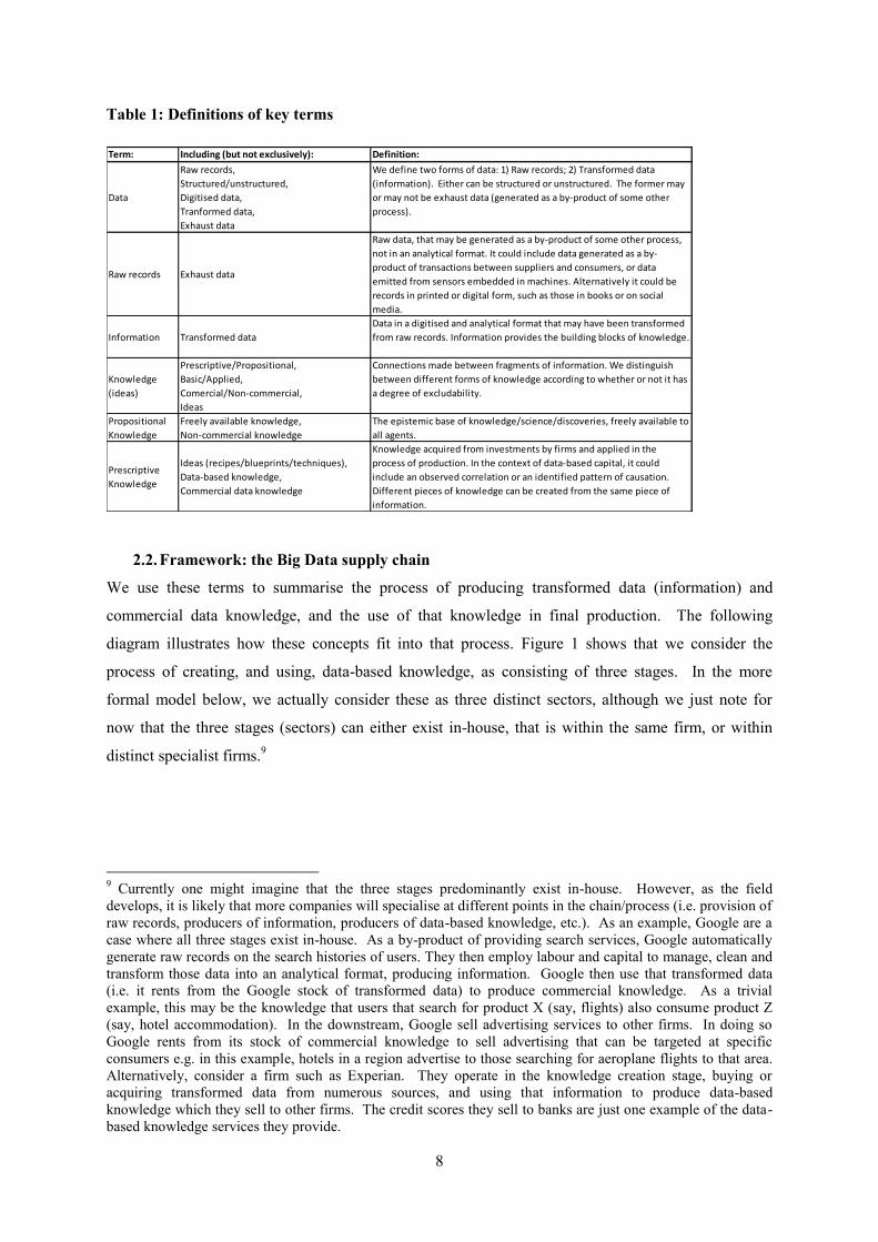
Table 1: Definitions of key terms
2.2. Framework: the Big Data supply chain
We use these terms to summarise the process of producing transformed data (information) and
commercial data knowledge, and the use of that knowledge in final production. The following
diagram illustrates how these concepts fit into that process. Figure 1 shows that we consider the
process of creating, and using, data-based knowledge, as consisting of three stages. In the more
formal model below, we actually consider these as three distinct sectors, although we just note for
now that the three stages (sectors) can either exist in-house, that is within the same firm, or within
distinct specialist firms.9
9 Currently one might imagine that the three stages predominantly exist in-house. However, as the field develops, it is likely that more companies will specialise at different points in the chain/process (i.e. provision of raw records, producers of information, producers of data-based knowledge, etc.). As an example, Google are a case where all three stages exist in-house. As a by-product of providing search services, Google automatically generate raw records on the search histories of users. They then employ labour and capital to manage, clean and transform those data into an analytical format, producing information. Google then use that transformed data (i.e. it rents from the Google stock of transformed data) to produce commercial knowledge. As a trivial example, this may be the knowledge that users that search for product X (say, flights) also consume product Z (say, hotel accommodation). In the downstream, Google sell advertising services to other firms. In doing so Google rents from its stock of commercial knowledge to sell advertising that can be targeted at specific consumers e.g. in this example, hotels in a region advertise to those searching for aeroplane flights to that area. Alternatively, consider a firm such as Experian. They operate in the knowledge creation stage, buying or acquiring transformed data from numerous sources, and using that information to produce data-based knowledge which they sell to other firms. The credit scores they sell to banks are just one example of the data-based knowledge services they provide.
Term: Including (but not exclusively): Definition:
Data
Raw records,
Structured/unstructured,
Digitised data,
Tranformed data,
Exhaust data
We define two forms of data: 1) Raw records; 2) Transformed data
(information). Either can be structured or unstructured. The former may
or may not be exhaust data (generated as a by-product of some other
process).
Raw records Exhaust data
Raw data, that may be generated as a by-product of some other process,
not in an analytical format. It could include data generated as a by-
product of transactions between suppliers and consumers, or data
emitted from sensors embedded in machines. Alternatively it could be
records in printed or digital form, such as those in books or on social
media.
Information Transformed data
Data in a digitised and analytical format that may have been transformed
from raw records. Information provides the building blocks of knowledge.
Knowledge
(ideas)
Prescriptive/Propositional,
Basic/Applied,
Comercial/Non-commercial,
Ideas
Connections made between fragments of information. We distinguish
between different forms of knowledge according to whether or not it has
a degree of excludability.
Propositional
Knowledge
Freely available knowledge,
Non-commercial knowledge
The epistemic base of knowledge/science/discoveries, freely available to
all agents.
Prescriptive
Knowledge
Ideas (recipes/blueprints/techniques),
Data-based knowledge,
Commercial data knowledge
Knowledge acquired from investments by firms and applied in the
process of production. In the context of data-based capital, it could
include an observed correlation or an identified pattern of causation.
Different pieces of knowledge can be created from the same piece of
information.
9
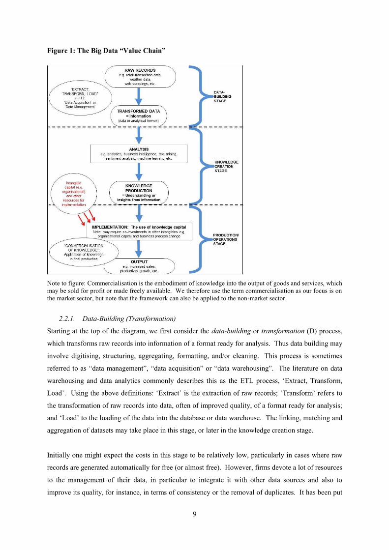
Figure 1: The Big Data “Value Chain”
Note to figure: Commercialisation is the embodiment of knowledge into the output of goods and services, which may be sold for profit or made freely available. We therefore use the term commercialisation as our focus is on the market sector, but note that the framework can also be applied to the non-market sector.
2.2.1. Data-Building (Transformation)
Starting at the top of the diagram, we first consider the data-building or transformation (D) process,
which transforms raw records into information of a format ready for analysis. Thus data building may
involve digitising, structuring, aggregating, formatting, and/or cleaning. This process is sometimes
referred to as “data management”, “data acquisition” or “data warehousing”. The literature on data
warehousing and data analytics commonly describes this as the ETL process, ‘Extract, Transform,
Load’. Using the above definitions: ‘Extract’ is the extraction of raw records; ‘Transform’ refers to
the transformation of raw records into data, often of improved quality, of a format ready for analysis;
and ‘Load’ to the loading of the data into the database or data warehouse. The linking, matching and
aggregation of datasets may take place in this stage, or later in the knowledge creation stage.
Initially one might expect the costs in this stage to be relatively low, particularly in cases where raw
records are generated automatically for free (or almost free). However, firms devote a lot of resources
to the management of their data, in particular to integrate it with other data sources and also to
improve its quality, for instance, in terms of consistency or the removal of duplicates. It has been put
10
to us that the “acquisition” or data-building process actually represents around 60-80% of the total
costs of producing data-based knowledge.10,11
2.2.2. Knowledge creation
The next stage is the knowledge creation (N) process, more commonly referred to as ‘data analytics’.
This stage takes the output of the data-building stage, and uses that data/information to conduct
analysis. That analysis could take a number of forms. It will include activities commonly referred to
in the literature as ‘data science’, ‘data/text mining’, ‘knowledge recovery’, ‘business intelligence’
and ‘machine learning’, with the latter referring to the use of artificial intelligence to discover
correlations in data. Whatever the method, the output of the analytics process is a piece of
commercial knowledge formed from the analysis of information, and used to construct advice to be
implemented in the final production of goods and services.
2.2.3. Downstream production of final goods and services
The final stage incorporates the application of knowledge in the production of final goods and
services, in the downstream production (operations) sector. We emphasise that the downstream is a
pure operations sector, that does not invest or create any form of capital, but just employs labour and
(tangible and intangible) capital to deliver final goods and services. Therefore, use of data-based
knowledge in the downstream does not equate to investment in the downstream. The downstream is a
pure using sector, with all investment occurring in the upstream.
However, implementation of data-based knowledge in downstream production may require co-
investments in other forms of intangible capital such as organisational (business process change) or
reputational (brand) capital. There are of course other upstreams that create other forms of intangible
capital also used in downstream production. But we do not seek to measure those here. Rather, our
focus is on the measurement of the data-building and data-based knowledge creation upstreams. For
estimates of a fuller range of intangible investment by industry, see Goodridge, Haskel et al. (2014).
As noted above, the upstream stages may either be situated in-house or in specialist firms operating
along the value chain presented in Figure 1. In the case where these stages exist in-house, the
downstream operations unit will receive advice from the upstream knowledge creation unit, located in
the same firm, for which it must pay an implicit but unobserved rental, just as the knowledge creation
10 We thank Rashik Parmar of IBM and Christopher Royles of Oracle for insights around the process of data transformation and data-based knowledge creation, and discussion around the value chain presented in Figure 1. 11 For instance, consider the spellchecker and autocomplete functions developed by Google, based on the searches entered by users. The raw data is provided for free by users, but transforming that raw data into information and ultimately knowledge is a costly process: a Google engineer claims that the system likely cost more to develop than the Microsoft system, which is based on records in dictionaries (Mayer-Schönberger and Cukier 2013).
11
stage must pay a rental for the use of transformed data.12. In the case where these stages exist in
distinct firms, the knowledge (or advice) could be sold to the downstream firm for an explicit fee, just
as plant and machinery is typically sold for an observed price. Alternatively a firm may buy in data
but conduct its own analytics, or generate its own data but outsource the analytics.
The downstream therefore receives advice formed on the basis of knowledge and takes action to
implement that knowledge in final production. For instance, it could be the knowledge that the cross-
promotion of goods results in increased sales, or it could be a re-optimisation of downstream
processes to improve productivity, based on say knowledge acquired from data emitted from sensors
embedded in machines. We refer to this implementation as the commercialisation of knowledge. The
term commercialisation obviously has connotations with the market and a profit motive. That is
because our primary focus here is on knowledge creation in the market sector. We emphasise
however that the framework can be applied more generally to the application of knowledge in non-
market production, such as in the delivery of public services.
2.3. Application of framework
2.3.1. Value in collection or use?
The literature around Big Data and data analytics frequently emphasises that the “value” of data lies
not in its collection but in its use. The framework makes clear that the demand for data is a derived
demand from the downstream production sector via the knowledge sector, just as the demand for oil is
a derived demand from the energy and transport sector. And the impact (or contribution) of data
occurs in the downstream delivery of goods and services. But data can potentially command a price
at any stage of the process, just as oil can. The question of what price is set out below.
2.3.2. Data versus knowledge
The framework suggests that data, and the knowledge gleaned from data, benefits downstream
productivity only if that knowledge is commercialised and applied in final production. The results of
Bakhshi, Bravo-Biosca et al. (2014) are supportive of this. They find that it is data analytics that has
the strongest link with firm performance and productivity, rather than just the collection of data. In
our model, it is the application of commercial data-based knowledge that contributes to downstream
productivity. Therefore we would only expect a productivity benefit if firms invest in knowledge
creation (analytics) as well as data-building (data management/acquisition).
12 The treatment is therefore perfectly symmetrical with purchased tangible capital (i.e. buildings, machinery etc.), for which a firm pays an implicit but unobserved annual rental for use of the asset.
12
2.3.3. Big data .vs. Little data
Above we have defined ‘data’, ‘information’, ‘ideas’ and ‘knowledge’. It may have been noticed that
we have not defined ‘Big Data’. Commonly used definitions of Big Data typically refer to the “3
V’s”, that is the large volume, variety and velocity of data that is being created, largely as a result of
the spread of the digital economy. But in this paper we are primarily concerned with investments in
data-building and data analytics that generate knowledge to be used in final production. The volume,
source, variety and type of data employed, or the speed with which it is generated, is less of a concern.
It therefore does not seem helpful to introduce a distinction between ‘big’ and ‘little’ data, after all,
each are based on the same foundations, that is mathematics, statistics, computer science etc. Further,
data and data analytics have been around for many years, and were making contributions to final
production long before the term ‘Big Data’ became so widespread, even if some of the techniques,
tools, technologies and approaches are new. For example, the major supermarket chains have been
collecting data on their customers purchasing patterns and preferences for some time. That activity
has just been made easier and richer with the new types of data that are becoming available and which
they can link to. Similarly insurance companies, who seek to create risk profiles of actual or potential
customers, and banks who use credit scores to assess customer applications for their products.
What matters then in this framework are the applicable business insights from analysing data. We
therefore see the emergence of the field of Big Data analytics as growth in an activity that has long
existed. The 3 V’s mean many more raw records are available and more information can be created,
facilitating growth in the data-building and knowledge creation sectors. This is not a change to the
process in the diagram, but rather a possible change to the underlying technical progress and
economies of scope and scale that might be available.13 Therefore we need to develop a framework
that allows us to analyse such changes which we do below.
3. Economic Framework
The previous section defined the terms that underlie our framework and presented an informal
exposition of the processes of data transformation, knowledge creation and commercialisation. In this
section we present a model of the payments and productivity underlying that process. The model
explicitly treats transformed data (information) and data-based knowledge as capital assets in a
national accounting and growth-accounting framework. For a justification of their treatment as
capital goods, please see Goodridge and Haskel (2015a).
13 For instance, new techniques in data management imply technical progress in the data-building stage. New techniques in analytics imply technical progress in the knowledge creation stage. New tools, such as various forms of open-source software freely available to upstream investors (e.g. Hadoop, R etc.) imply technical progress in both upstream stages.
13
3.1. A formal model
The framework presented here is analogous to the upstream-downstream framework presented in
Corrado, Goodridge et al. (2011). The main difference is that here we consider two upstream sectors:
the data-building (transformation) sector (“D”) and the knowledge creation sector (“N”). We
emphasise that the upstream can of course exist in-house. We show how various statistics on Big
Data fit into the framework, and further how we can apply the framework to the measurement of
investment in data transformation and data analytics and the contribution they make to growth.
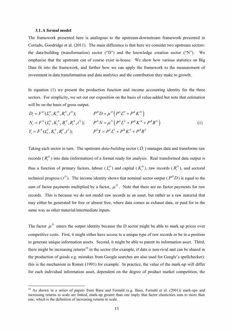
In equation (1) we present the production function and income accounting identity for the three
sectors. For simplicity, we set out our exposition on the basis of value-added but note that estimation
will be on the basis of gross output.
( , , , );
( , , , , );
( , , , );
D D D D D D D L D K D
t t t t
N N N N N N N N L N K N B N
t t t t t
Y Y Y Y Y Y L Y K Y R Y
t t t t
D F L K R t P D P L P K
N F L K B R t P N P L P K P B
Y F L K R t P Y P L P K P R
(1)
Taking each sector in turn. The upstream data-building sector ( tD ) manages data and transforms raw
records (D
tR ) into data (information) of a format ready for analysis. Real transformed data output is
thus a function of primary factors, labour (D
tL ) and capital (D
tK ), raw records (D
tR ), and sectoral
technical progress (Dt ). The income identity shows that nominal sector output (
DP D ) is equal to the
sum of factor payments multiplied by a factor, D . Note that there are no factor payments for raw
records. This is because we do not model raw records as an asset, but rather as a raw material that
may either be generated for free or almost free, where data comes as exhaust data, or paid for in the
same way as other material/intermediate inputs.
The factor D enters the output identity because the D sector might be able to mark up prices over
competitive costs. First, it might either have access to a unique type of raw records or be in a position
to generate unique information assets. Second, it might be able to patent its information asset. Third,
there might be increasing returns14 in the sector (for example, if data is non-rival and can be shared in
the production of goods e.g. mistakes from Google searches are also used for Google’s spellchecker):
this is the mechanism in Romer (1991) for example. In practice, the value of the mark-up will differ
for each individual information asset, dependent on the degree of product market competition, the
14 As shown in a series of papers from Basu and Fernald (e.g. Basu, Fernald et al. (2001)) mark-ups and increasing returns to scale are linked, mark-up greater than one imply that factor elasticities sum to more than one, which is the definition of increasing returns to scale.
14
scarcity of that information, and its commercial value to ultimate users. Of course the acquisition and
maintenance of this market power provides a further incentive for the upstream to exist in-house. 15
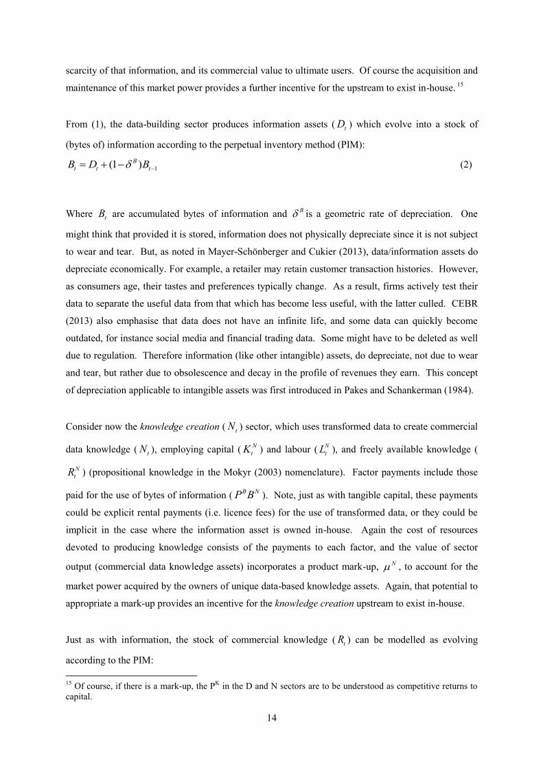
From (1), the data-building sector produces information assets ( tD ) which evolve into a stock of
(bytes of) information according to the perpetual inventory method (PIM):
1(1 )B
t t tB D B (2)
Where tB are accumulated bytes of information and B is a geometric rate of depreciation. One
might think that provided it is stored, information does not physically depreciate since it is not subject
to wear and tear. But, as noted in Mayer-Schönberger and Cukier (2013), data/information assets do
depreciate economically. For example, a retailer may retain customer transaction histories. However,
as consumers age, their tastes and preferences typically change. As a result, firms actively test their
data to separate the useful data from that which has become less useful, with the latter culled. CEBR
(2013) also emphasise that data does not have an infinite life, and some data can quickly become
outdated, for instance social media and financial trading data. Some might have to be deleted as well
due to regulation. Therefore information (like other intangible) assets, do depreciate, not due to wear
and tear, but rather due to obsolescence and decay in the profile of revenues they earn. This concept
of depreciation applicable to intangible assets was first introduced in Pakes and Schankerman (1984).
Consider now the knowledge creation ( tN ) sector, which uses transformed data to create commercial
data knowledge ( tN ), employing capital (N
tK ) and labour (N
tL ), and freely available knowledge (
N
tR ) (propositional knowledge in the Mokyr (2003) nomenclature). Factor payments include those
paid for the use of bytes of information (B NP B ). Note, just as with tangible capital, these payments
could be explicit rental payments (i.e. licence fees) for the use of transformed data, or they could be
implicit in the case where the information asset is owned in-house. Again the cost of resources
devoted to producing knowledge consists of the payments to each factor, and the value of sector
output (commercial data knowledge assets) incorporates a product mark-up, N , to account for the
market power acquired by the owners of unique data-based knowledge assets. Again, that potential to
appropriate a mark-up provides an incentive for the knowledge creation upstream to exist in-house.
Just as with information, the stock of commercial knowledge ( tR ) can be modelled as evolving
according to the PIM:
15 Of course, if there is a mark-up, the PK in the D and N sectors are to be understood as competitive returns to capital.
15
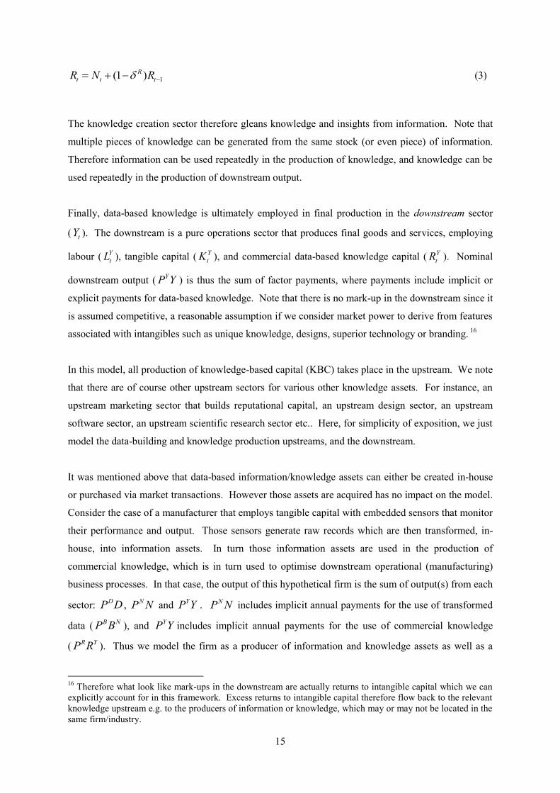
1(1 )R
t t tR N R (3)
The knowledge creation sector therefore gleans knowledge and insights from information. Note that
multiple pieces of knowledge can be generated from the same stock (or even piece) of information.
Therefore information can be used repeatedly in the production of knowledge, and knowledge can be
used repeatedly in the production of downstream output.
Finally, data-based knowledge is ultimately employed in final production in the downstream sector
( tY ). The downstream is a pure operations sector that produces final goods and services, employing
labour (Y
tL ), tangible capital (Y
tK ), and commercial data-based knowledge capital (Y
tR ). Nominal
downstream output (YP Y ) is thus the sum of factor payments, where payments include implicit or
explicit payments for data-based knowledge. Note that there is no mark-up in the downstream since it
is assumed competitive, a reasonable assumption if we consider market power to derive from features
associated with intangibles such as unique knowledge, designs, superior technology or branding. 16
In this model, all production of knowledge-based capital (KBC) takes place in the upstream. We note
that there are of course other upstream sectors for various other knowledge assets. For instance, an
upstream marketing sector that builds reputational capital, an upstream design sector, an upstream
software sector, an upstream scientific research sector etc.. Here, for simplicity of exposition, we just
model the data-building and knowledge production upstreams, and the downstream.
It was mentioned above that data-based information/knowledge assets can either be created in-house
or purchased via market transactions. However those assets are acquired has no impact on the model.
Consider the case of a manufacturer that employs tangible capital with embedded sensors that monitor
their performance and output. Those sensors generate raw records which are then transformed, in-
house, into information assets. In turn those information assets are used in the production of
commercial knowledge, which is in turn used to optimise downstream operational (manufacturing)
business processes. In that case, the output of this hypothetical firm is the sum of output(s) from each
sector: DP D ,
NP N and YP Y .
NP N includes implicit annual payments for the use of transformed
data (B NP B ), and
YP Y includes implicit annual payments for the use of commercial knowledge
(R YP R ). Thus we model the firm as a producer of information and knowledge assets as well as a
16 Therefore what look like mark-ups in the downstream are actually returns to intangible capital which we can explicitly account for in this framework. Excess returns to intangible capital therefore flow back to the relevant knowledge upstream e.g. to the producers of information or knowledge, which may or may not be located in the same firm/industry.

16
producer of manufactured final goods. The output of assets (here DP D and
NP N ) are related to the
factor payments for their use via the Hall-Jorgenson user costs relation (Hall and Jorgenson 1967):
( )
( )
B D B D
R N R N
P P r
and
P P r
(4)
Where r is the economy-wide nominal net rate of return to capital and accounts for capital
(holding) gains/losses from changes in the asset price. Asset-level factor payments (or capital
compensation) therefore consist of a net return to capital plus depreciation, minus any holding gain,
with all these components directly proportional to the nominal value of the stock (D NP B or
N YP R ).
3.1.1. Relation with GDP
Total value-added is the sum of value added earned in each sector. With no intermediates, this is then
the sum of each sector’s output i.e. the output of final consumer and (tangible/intangible) investment
goods, or equivalently from the income side, the sum of factor payments to labour and all forms of
capital. Therefore in this economy of three sectors, value-added can be written as:17
Q D N Y
L K B R
P Q P D P N P Y
P L P K P B P R
(5)
Where:
L L D L N L Y
K K D K N K Y
P L P L P L P L
P K P K P K P K
(6)
Before moving onto the measurement of real output, it is worth saying a little more about upstream
inputs in (1). Of course there is labour input (LP L ) from the kinds of occupations that are receiving
more and more attention, such as ‘data scientists’, ‘data engineers’ and ‘business intelligence
analysts’. In the data-building (D) sector, we would expect to find occupations such as ‘data
administrators’, ‘data managers’, ‘data engineers’ and workers in ‘data control’. The knowledge
creation (N) sector is more likely to include occupations such as ‘data scientists’, ‘business
17 Note, there is a slight complication here. In the above framework (e.g equation (1)) the PK term represents the competitive cost of capital were it observed. Since, in practice, capital compensation is estimated residually, then (5) holds but the cost of capital incorporates mark-ups which manifest as above-competitive returns to capital.
17
intelligence’ and ‘data/statistical analysts’.18 In practice, the roles of some workers/occupations could
include some aspects of both data-building and knowledge creation.
There is also capital input (KP K ), which might include buildings and computer hardware for
instance. Upstream capital will also include software, used intensively in the creation of information
and the gleaning of data-based knowledge. However, a noted feature of data warehousing and data
analytics is the widespread use of various forms of open-source software, such as Hadoop, NoSQL
and R. Since there are typically no payments for the use of such software, their contribution does not
appear in the nominal data. Rather they act to increase upstream TFP and real upstream output. The
measurement of real upstream output and TFP are discussed in the next sub-section.
3.2. Contribution to growth in theory
With the exception of the PIM, most of the above identities are based on nominal flows. But to say
something about the contribution of (transformed) data and data-based knowledge to growth in output
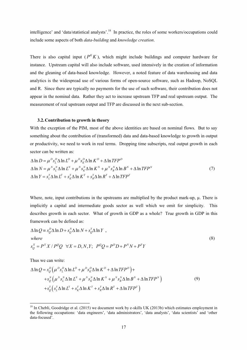
or productivity, we need to work in real terms. Dropping time subscripts, real output growth in each
sector can be written as:
ln ln ln ln
ln ln ln ln ln
ln ln ln ln ln
D D D D D D D
L K
N N N N N N N N N N
L K B
Y Y Y Y Y Y Y
L K R
D s L s K TFP
N s L s K s B TFP
Y s L s K s R TFP
(7)
Where, note, input contributions in the upstreams are multiplied by the product mark-up, µ. There is
implicitly a capital and intermediate goods sector as well which we omit for simplicity. This
describes growth in each sector. What of growth in GDP as a whole? True growth in GDP in this
framework can be defined as:
ln ln ln ln ,
/ , , ;
D N Y
Q Q Q
X X Q Q D N Y
Q
Q s D s N s Y
where
s P X P Q X D N Y P Q P D P N P Y
(8)
Thus we can write:
ln ln ln ln
ln ln ln ln
ln ln ln ln
D D D D D D D D
Q L K
N N N N N N N N N N N
Q L K B
Y Y Y Y Y Y Y Y
Q L K R
Q s s L s K TFP
s s L s K s B TFP
s s L s K s R TFP
(9)
18 In Chebli, Goodridge et al. (2015) we document work by e-skills UK (2013b) which estimates employment in the following occupations: ‘data engineers’, ‘data administrators’, ‘data analysts’, ‘data scientists’ and ‘other data-focused’.
18
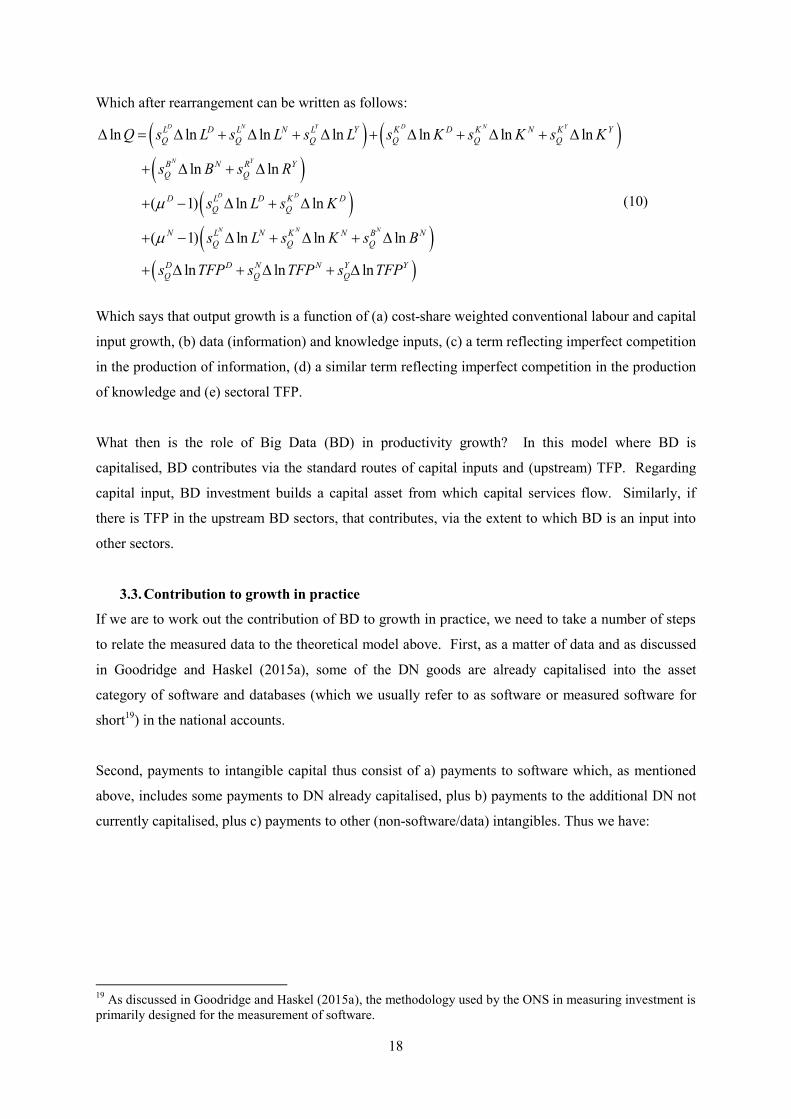
Which after rearrangement can be written as follows:
ln ln ln ln ln ln ln
ln ln
( 1) ln ln
( 1) ln ln ln
ln ln ln
D N Y D N Y
N Y
D D
N N N
L D L N L Y K D K N K Y
Q Q Q Q Q Q
B N R Y
Q Q
D L D K D
Q Q
N L N K N B N
Q Q Q
D D N N Y Y
Q Q Q
Q s L s L s L s K s K s K
s B s R
s L s K
s L s K s B
s TFP s TFP s TFP
(10)
Which says that output growth is a function of (a) cost-share weighted conventional labour and capital
input growth, (b) data (information) and knowledge inputs, (c) a term reflecting imperfect competition
in the production of information, (d) a similar term reflecting imperfect competition in the production
of knowledge and (e) sectoral TFP.
What then is the role of Big Data (BD) in productivity growth? In this model where BD is
capitalised, BD contributes via the standard routes of capital inputs and (upstream) TFP. Regarding
capital input, BD investment builds a capital asset from which capital services flow. Similarly, if
there is TFP in the upstream BD sectors, that contributes, via the extent to which BD is an input into
other sectors.
3.3. Contribution to growth in practice
If we are to work out the contribution of BD to growth in practice, we need to take a number of steps
to relate the measured data to the theoretical model above. First, as a matter of data and as discussed
in Goodridge and Haskel (2015a), some of the DN goods are already capitalised into the asset
category of software and databases (which we usually refer to as software or measured software for
short19) in the national accounts.
Second, payments to intangible capital thus consist of a) payments to software which, as mentioned
above, includes some payments to DN already capitalised, plus b) payments to the additional DN not
currently capitalised, plus c) payments to other (non-software/data) intangibles. Thus we have:
19 As discussed in Goodridge and Haskel (2015a), the methodology used by the ONS in measuring investment is primarily designed for the measurement of software.
19
Measured software capital services
DN capital services within software Additional DN capital services
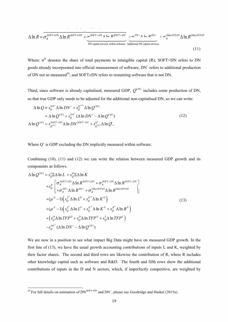
ln ln ln lnSOFT DN SOFT DN SOFT DN SOFT DN DN DN Othe
R R R RR R R R lnrINTAN OtherINTANR (11)
Where: R denotes the share of total payments to intangible capital (R); SOFT=DN refers to DN
goods already incorporated into official measurement of software; DN+ refers to additional production
of DN not so measured20; and SOFT≠DN refers to remaining software that is not DN.
Third, since software is already capitalised, measured GDP, ( )MQ includes some production of DN,
so that true GDP only needs to be adjusted for the additional non-capitalised DN, so we can write:
( )
( ) ( )
( )
( ) ( )
( )
ln ln ln
ln ( ln ln )
ln ln ln ,
M
M M
DN Q M
Q Q
M DN M
Q
M SOFT DN SOFT DN Q
Q Q
Q s DN s Q
Q s DN Q
Q s DN s Q
(12)
Where Q’ is GDP excluding the DN implicitly measured within software.
Combining (10), (11) and (12) we can write the relation between measured GDP growth and its
components as follows.
( )ln ln ln
ln ln
ln ln
( 1) ln ln
( 1) ln ln ln
ln ln
D D
N N N
M L K
Q Q
SOFT DN SOFT DN SOFT DN SOFT DN
R RR
Q DN DN OtherINTAN OtherINTAN
R R
D L D K D
Q Q
N L N K N B N
Q Q Q
D D D
Q Q
Q s L s K
R Rs
R R
s L s K
s L s K s B
s TFP s TF
( )
ln
( ln ln )
N Y Y
Q
DN M
Q
P s TFP
s DN Q
(13)
We are now in a position to see what impact Big Data might have on measured GDP growth. In the
first line of (13), we have the usual growth accounting contributions of inputs L and K, weighted by
their factor shares. The second and third rows are likewise the contribution of R, where R includes
other knowledge capital such as software and R&D. The fourth and fifth rows show the additional
contributions of inputs in the D and N sectors, which, if imperfectly competitive, are weighted by
20 For full details on estimation of DNSOFT=DN and DN+, please see Goodridge and Haskel (2015a).
20
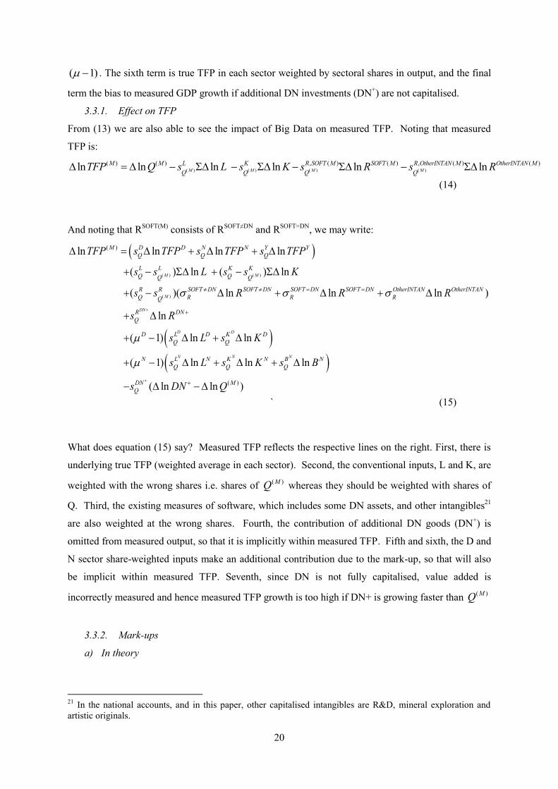
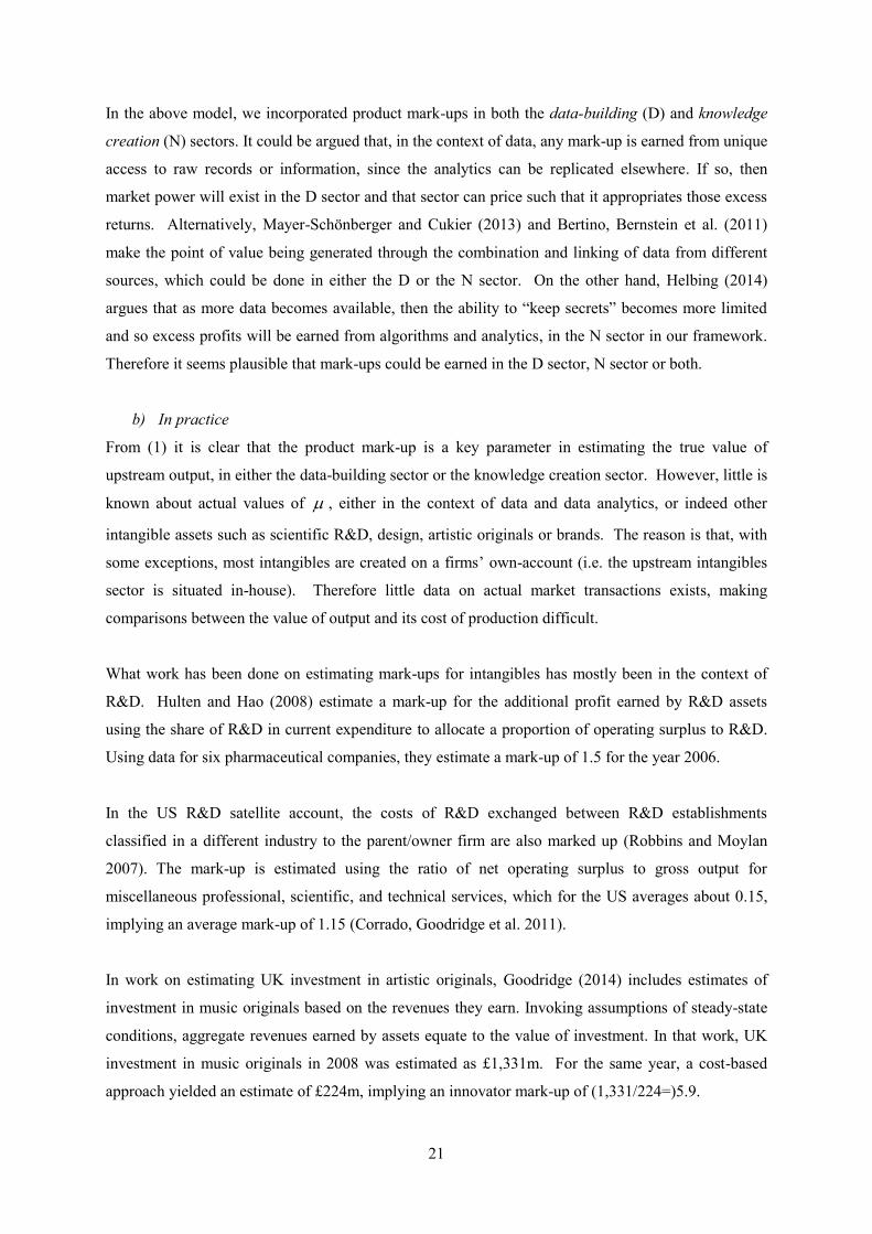
( 1) . The sixth term is true TFP in each sector weighted by sectoral shares in output, and the final
term the bias to measured GDP growth if additional DN investments (DN+) are not capitalised.
3.3.1. Effect on TFP
From (13) we are also able to see the impact of Big Data on measured TFP. Noting that measured
TFP is:
( ) ( ) ( ) ( )
( ) ( ) , ( ) ( ) , ( ) ( )ln ln ln ln ln lnM M M M
M M L K R SOFT M SOFT M R OtherINTAN M OtherINTAN M
Q Q Q QTFP Q s L s K s R s R
(14)
And noting that RSOFT(M) consists of RSOFT≠DN and RSOFT=DN, we may write:
( ) ( )
( )
( )ln ln ln ln
( ) ln ( ) ln
( )( ln ln ln )
ln
( 1) ln ln
M M
M
DN
D D
M D D N N Y Y
Q Q Q
L L K K
Q QQ Q
R R SOFT DN SOFT DN SOFT DN SOFT DN OtherINTAN OtherINTAN
Q R R RQ
R DN
Q
D L D K
Q Q
TFP s TFP s TFP s TFP
s s L s s K
s s R R R
s R
s L s K
( )
( 1) ln ln ln
( ln ln )
N N N
D
N L N K N B N
Q Q Q
DN M
Q
s L s K s B
s DN Q
` (15)
What does equation (15) say? Measured TFP reflects the respective lines on the right. First, there is
underlying true TFP (weighted average in each sector). Second, the conventional inputs, L and K, are
weighted with the wrong shares i.e. shares of ( )MQ whereas they should be weighted with shares of
Q. Third, the existing measures of software, which includes some DN assets, and other intangibles21
are also weighted at the wrong shares. Fourth, the contribution of additional DN goods (DN+) is
omitted from measured output, so that it is implicitly within measured TFP. Fifth and sixth, the D and
N sector share-weighted inputs make an additional contribution due to the mark-up, so that will also
be implicit within measured TFP. Seventh, since DN is not fully capitalised, value added is
incorrectly measured and hence measured TFP growth is too high if DN+ is growing faster than ( )MQ
3.3.2. Mark-ups
a) In theory
21 In the national accounts, and in this paper, other capitalised intangibles are R&D, mineral exploration and artistic originals.
21
In the above model, we incorporated product mark-ups in both the data-building (D) and knowledge
creation (N) sectors. It could be argued that, in the context of data, any mark-up is earned from unique
access to raw records or information, since the analytics can be replicated elsewhere. If so, then
market power will exist in the D sector and that sector can price such that it appropriates those excess
returns. Alternatively, Mayer-Schönberger and Cukier (2013) and Bertino, Bernstein et al. (2011)
make the point of value being generated through the combination and linking of data from different
sources, which could be done in either the D or the N sector. On the other hand, Helbing (2014)
argues that as more data becomes available, then the ability to “keep secrets” becomes more limited
and so excess profits will be earned from algorithms and analytics, in the N sector in our framework.
Therefore it seems plausible that mark-ups could be earned in the D sector, N sector or both.
b) In practice
From (1) it is clear that the product mark-up is a key parameter in estimating the true value of
upstream output, in either the data-building sector or the knowledge creation sector. However, little is
known about actual values of , either in the context of data and data analytics, or indeed other
intangible assets such as scientific R&D, design, artistic originals or brands. The reason is that, with
some exceptions, most intangibles are created on a firms’ own-account (i.e. the upstream intangibles
sector is situated in-house). Therefore little data on actual market transactions exists, making
comparisons between the value of output and its cost of production difficult.
What work has been done on estimating mark-ups for intangibles has mostly been in the context of
R&D. Hulten and Hao (2008) estimate a mark-up for the additional profit earned by R&D assets
using the share of R&D in current expenditure to allocate a proportion of operating surplus to R&D.
Using data for six pharmaceutical companies, they estimate a mark-up of 1.5 for the year 2006.
In the US R&D satellite account, the costs of R&D exchanged between R&D establishments
classified in a different industry to the parent/owner firm are also marked up (Robbins and Moylan
2007). The mark-up is estimated using the ratio of net operating surplus to gross output for
miscellaneous professional, scientific, and technical services, which for the US averages about 0.15,
implying an average mark-up of 1.15 (Corrado, Goodridge et al. 2011).
In work on estimating UK investment in artistic originals, Goodridge (2014) includes estimates of
investment in music originals based on the revenues they earn. Invoking assumptions of steady-state
conditions, aggregate revenues earned by assets equate to the value of investment. In that work, UK
investment in music originals in 2008 was estimated as £1,331m. For the same year, a cost-based
approach yielded an estimate of £224m, implying an innovator mark-up of (1,331/224=)5.9.
22
A similar approach can be taken to estimating a mark-up for broadcasting originals. ITV is a UK
commercial broadcaster that earns revenues from the sale of advertising carried on its broadcasts. An
approximate mark-up for ITV originals can be estimated using data on ITV costs of television
production and the revenues generated through the sale of advertising. Data from OFCOM (2013)
show that in 2012 ITV costs of production were £814m. Data from the ITV Annual Report show that
net advertising revenues were £1,510m (ITV 2013), implying a mark-up of (1,510/814=)1.86.
4. Information and Data-Based Knowledge as assets
The above framework modelled information and data-based knowledge as assets that make long-lived
contributions to production. It is therefore worth saying a little more about the justification for their
treatment as assets, including a discussion of official capitalisation criteria as set out in the SNA.
4.1. Do information and commercial data knowledge function as assets?
To assess whether or not (transformed) data and commercial data knowledge ought to be counted as
assets, and whether the expenditures towards their creation ought to be counted as investments, it is
worth reminding ourselves of the definitions of capital and investment.
As pointed out in Jorgenson and Griliches (1967) and Hulten (1979), savings and investment are a
means of sacrificing current consumption in order to increase future consumption, making the
appropriate definition of economic investment the devotion of current resources to the pursuit of
future returns (Weitzman 1976; Hulten 1979). Consistent application of that definition immediately
makes clear that whether expenditure is on a factory or a virtual data centre for long-term use does not
matter to the question of what ought to be classified as investment. What matters for the purposes of
capitalisation is whether data (information), and data-based knowledge, function as assets that
generate future returns and make long-lived contributions to production. As noted in CEBR (2013),
data that enables firms to derive future economic benefits ought to be regarded as assets
Evidence for the contribution of data and data-based knowledge to productivity can be found in
Brynjolfsson, Hitt et al. (2011). Using firm-level data on business practices and controlling for
traditional capital including ICT, those authors find that the use of data-driven decisionmaking (DDD)
can explain a 5-6% increase in firm output and productivity and is also associated with significantly
higher firm profitability and market value, with potential issues around reverse causality addressed
using instrumental variable techniques. Similarly, using data from a NESTA survey on data activity,
Bakhshi, Bravo-Biosca et al. (2014) find that data active firms are on average 8% more productive
than their counterparts. The same authors also report strong links between data analytics and firm
23
productivity, with firms that empower employees to implement insights gleaned from data found to be
16% more productive. Further support for the capitalisation of data can be found in: Economist
Intelligence Unit (2012), which reports results of a survey of managers who on average stated that
(big) data had improved their organisations performance by 26% over the past three years; Davenport
and Harris (2007), who make the link between use of data analytics and acquiring a competitive
advantage; and LaValle, Hopkins et al. (2010) who show that firms that employ data analytics are
twice as likely to be among the industry top performers.
To help underline how data and data-based knowledge function as assets, Goodridge and Haskel
(2015a) report on case studies for the retail, manufacturing and telecommunications sectors. Those
studies provide examples of applications, or potential applications, of data and data analytics in
market production, as reported in Manyika, Chui et al. (2011) and OECD (2013), where data is used
to create data-based knowledge which in turn is applied in downstream production, increasing
productivity by either: a) improving efficiency and reducing costs; or b) by adding to the
quantity/quality of goods and services produced, thereby increasing output.
4.2. System of National Accounts (SNA)
SNA investment criteria have the same interpretation as those from the economic literature set out
above. If an input contributes to production over more than one accounting period, its acquisition
ought to be counted as investment.22 The SNA describes intellectual property products (IPPs) as
assets that are “the result of research, development, investigation or innovation leading to knowledge
that the developers can market or use to their own benefit in production”, and states that such
knowledge remains an asset until it is ether no longer protected or becomes obsolete. We note that
provided they are repeatedly used over more than one accounting period, transformed data
(information) and commercial data knowledge meet the SNA definitions for both assets and, more
specifically, IPPs. However, some features of data and databases, namely that data is, in national
accounts nomenclature, a non-produced asset, have implications for measurement. We expand on this
issue, and SNA criteria in general, in Appendix 1.
5. Growth-accounting
In this paper we undertake growth accounting for the UK market sector based on a value-added
production function that incorporates intangible capital, and specifically data-based capital. As
described in Goodridge and Haskel (2015a), investments in data are defined to include the building
and transformation of data, and the extraction of knowledge from data.
22 Where acquisition can include the purchase of an asset in a market transaction, or own-account (in-house) asset production.
24
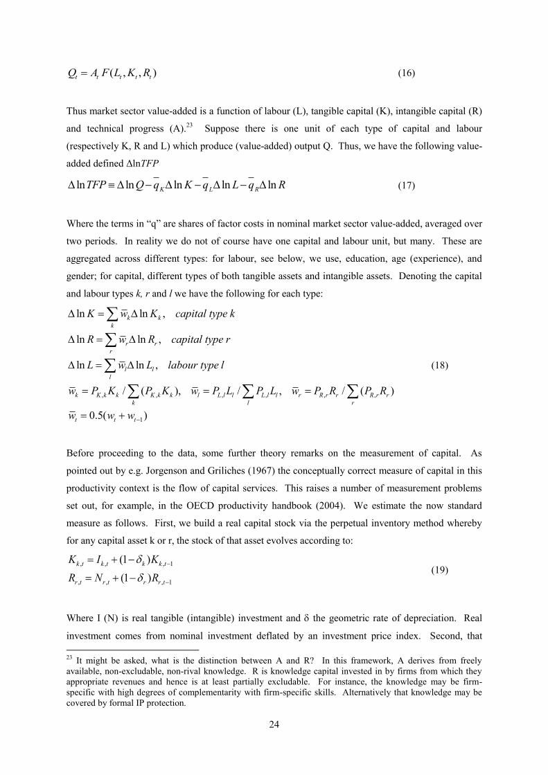
( , , )t t t t tQ A F L K R (16)
Thus market sector value-added is a function of labour (L), tangible capital (K), intangible capital (R)
and technical progress (A).23 Suppose there is one unit of each type of capital and labour
(respectively K, R and L) which produce (value-added) output Q. Thus, we have the following value-
added defined ΔlnTFP
ln ln ln ln lnK L RTFP Q q K q L q R (17)
Where the terms in “q” are shares of factor costs in nominal market sector value-added, averaged over
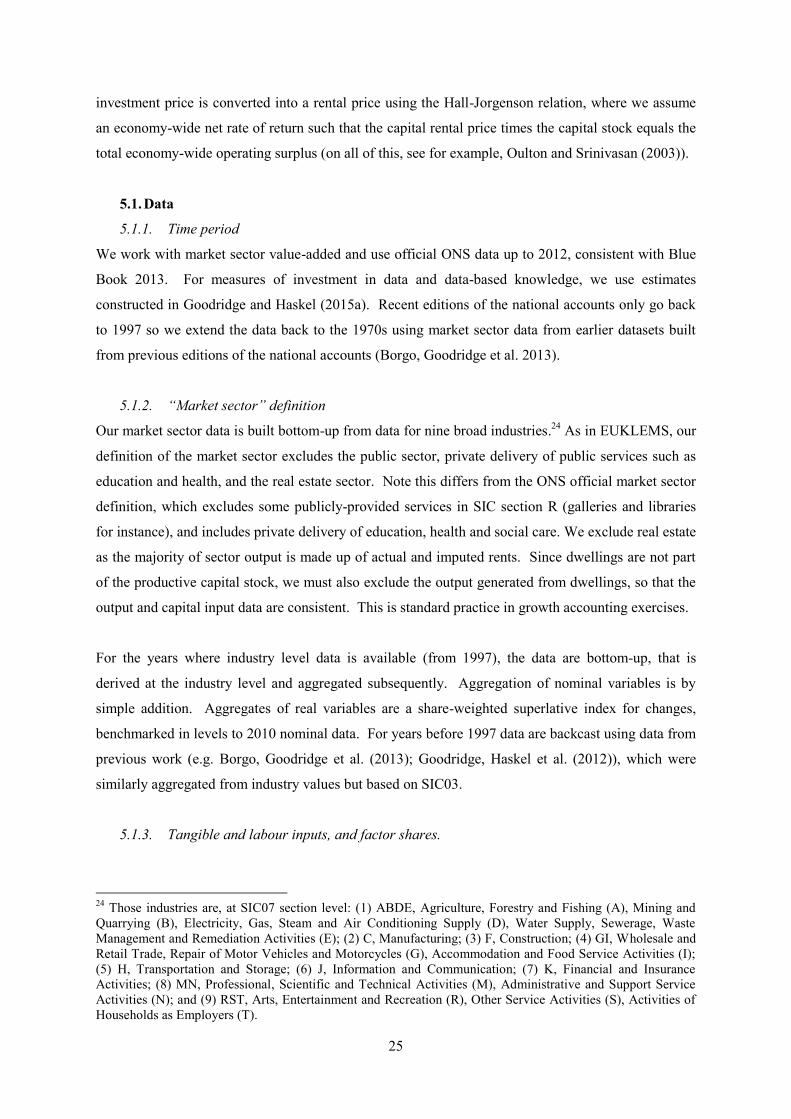
two periods. In reality we do not of course have one capital and labour unit, but many. These are
aggregated across different types: for labour, see below, we use, education, age (experience), and
gender; for capital, different types of both tangible assets and intangible assets. Denoting the capital
and labour types k, r and l we have the following for each type:
, , , , , ,
1
ln ln ,
ln ln ,
ln ln ,
/ ( ), / , / ( )
0.5( )
k k
k
r r
r
l l
l
k K k k K k k l L l l L l l r R r r R r r
k l r
t t t
K w K capital type k
R w R capital type r
L w L labour type l
w P K P K w P L P L w P R P R
w w w
(18)
Before proceeding to the data, some further theory remarks on the measurement of capital. As
pointed out by e.g. Jorgenson and Griliches (1967) the conceptually correct measure of capital in this
productivity context is the flow of capital services. This raises a number of measurement problems
set out, for example, in the OECD productivity handbook (2004). We estimate the now standard
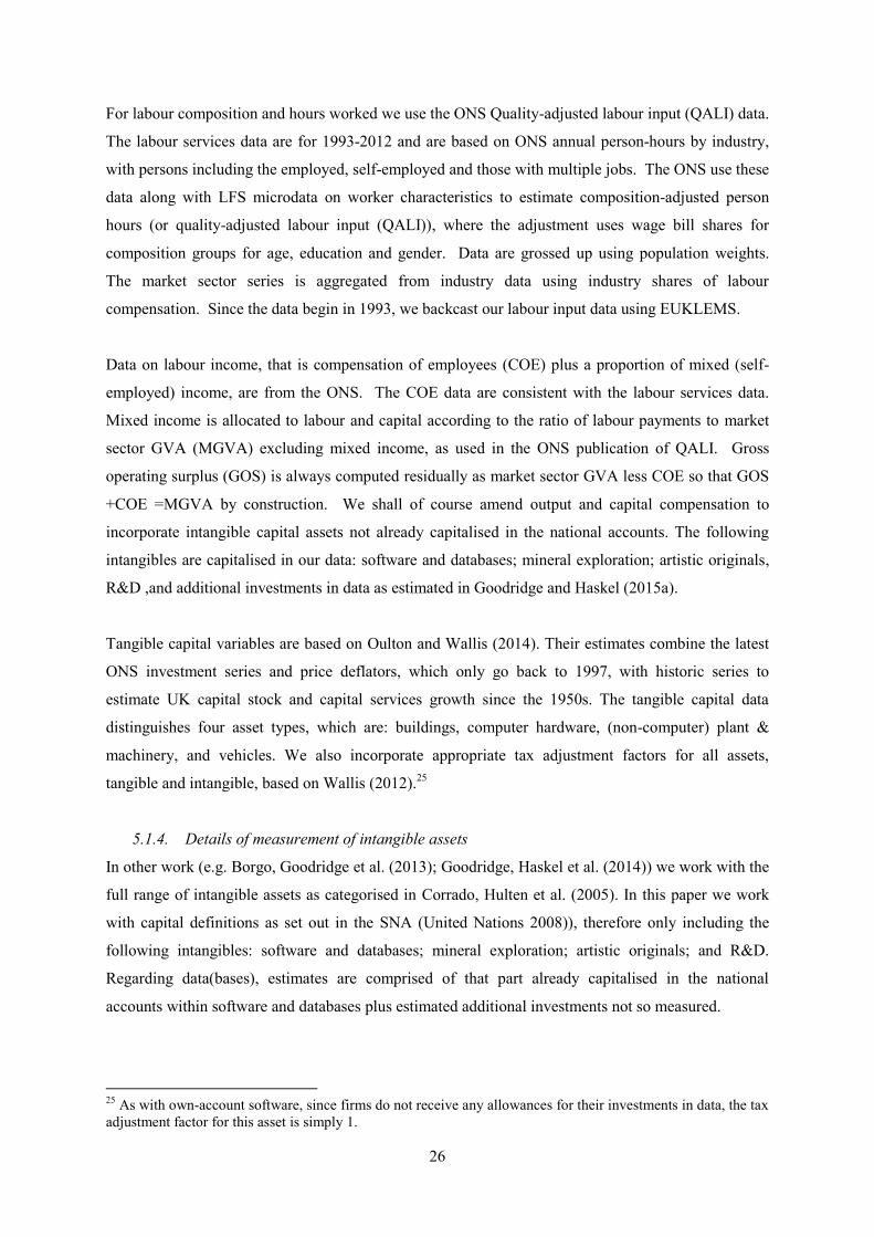
measure as follows. First, we build a real capital stock via the perpetual inventory method whereby
for any capital asset k or r, the stock of that asset evolves according to:
, , , 1
, , , 1
(1 )
(1 )
k t k t k k t
r t r t r r t
K I K
R N R
(19)
Where I (N) is real tangible (intangible) investment and the geometric rate of depreciation. Real
investment comes from nominal investment deflated by an investment price index. Second, that
23 It might be asked, what is the distinction between A and R? In this framework, A derives from freely available, non-excludable, non-rival knowledge. R is knowledge capital invested in by firms from which they appropriate revenues and hence is at least partially excludable. For instance, the knowledge may be firm-specific with high degrees of complementarity with firm-specific skills. Alternatively that knowledge may be covered by formal IP protection.
25
investment price is converted into a rental price using the Hall-Jorgenson relation, where we assume
an economy-wide net rate of return such that the capital rental price times the capital stock equals the
total economy-wide operating surplus (on all of this, see for example, Oulton and Srinivasan (2003)).
5.1. Data
5.1.1. Time period
We work with market sector value-added and use official ONS data up to 2012, consistent with Blue
Book 2013. For measures of investment in data and data-based knowledge, we use estimates
constructed in Goodridge and Haskel (2015a). Recent editions of the national accounts only go back
to 1997 so we extend the data back to the 1970s using market sector data from earlier datasets built
from previous editions of the national accounts (Borgo, Goodridge et al. 2013).
5.1.2. “Market sector” definition
Our market sector data is built bottom-up from data for nine broad industries.24 As in EUKLEMS, our
definition of the market sector excludes the public sector, private delivery of public services such as
education and health, and the real estate sector. Note this differs from the ONS official market sector
definition, which excludes some publicly-provided services in SIC section R (galleries and libraries
for instance), and includes private delivery of education, health and social care. We exclude real estate
as the majority of sector output is made up of actual and imputed rents. Since dwellings are not part
of the productive capital stock, we must also exclude the output generated from dwellings, so that the
output and capital input data are consistent. This is standard practice in growth accounting exercises.
For the years where industry level data is available (from 1997), the data are bottom-up, that is
derived at the industry level and aggregated subsequently. Aggregation of nominal variables is by
simple addition. Aggregates of real variables are a share-weighted superlative index for changes,
benchmarked in levels to 2010 nominal data. For years before 1997 data are backcast using data from
previous work (e.g. Borgo, Goodridge et al. (2013); Goodridge, Haskel et al. (2012)), which were
similarly aggregated from industry values but based on SIC03.
5.1.3. Tangible and labour inputs, and factor shares.
24 Those industries are, at SIC07 section level: (1) ABDE, Agriculture, Forestry and Fishing (A), Mining and Quarrying (B), Electricity, Gas, Steam and Air Conditioning Supply (D), Water Supply, Sewerage, Waste Management and Remediation Activities (E); (2) C, Manufacturing; (3) F, Construction; (4) GI, Wholesale and Retail Trade, Repair of Motor Vehicles and Motorcycles (G), Accommodation and Food Service Activities (I); (5) H, Transportation and Storage; (6) J, Information and Communication; (7) K, Financial and Insurance Activities; (8) MN, Professional, Scientific and Technical Activities (M), Administrative and Support Service Activities (N); and (9) RST, Arts, Entertainment and Recreation (R), Other Service Activities (S), Activities of Households as Employers (T).
26
For labour composition and hours worked we use the ONS Quality-adjusted labour input (QALI) data.
The labour services data are for 1993-2012 and are based on ONS annual person-hours by industry,
with persons including the employed, self-employed and those with multiple jobs. The ONS use these
data along with LFS microdata on worker characteristics to estimate composition-adjusted person
hours (or quality-adjusted labour input (QALI)), where the adjustment uses wage bill shares for
composition groups for age, education and gender. Data are grossed up using population weights.
The market sector series is aggregated from industry data using industry shares of labour
compensation. Since the data begin in 1993, we backcast our labour input data using EUKLEMS.
Data on labour income, that is compensation of employees (COE) plus a proportion of mixed (self-
employed) income, are from the ONS. The COE data are consistent with the labour services data.
Mixed income is allocated to labour and capital according to the ratio of labour payments to market
sector GVA (MGVA) excluding mixed income, as used in the ONS publication of QALI. Gross
operating surplus (GOS) is always computed residually as market sector GVA less COE so that GOS
+COE =MGVA by construction. We shall of course amend output and capital compensation to
incorporate intangible capital assets not already capitalised in the national accounts. The following
intangibles are capitalised in our data: software and databases; mineral exploration; artistic originals,
R&D ,and additional investments in data as estimated in Goodridge and Haskel (2015a).
Tangible capital variables are based on Oulton and Wallis (2014). Their estimates combine the latest
ONS investment series and price deflators, which only go back to 1997, with historic series to
estimate UK capital stock and capital services growth since the 1950s. The tangible capital data
distinguishes four asset types, which are: buildings, computer hardware, (non-computer) plant &
machinery, and vehicles. We also incorporate appropriate tax adjustment factors for all assets,
tangible and intangible, based on Wallis (2012).25
5.1.4. Details of measurement of intangible assets
In other work (e.g. Borgo, Goodridge et al. (2013); Goodridge, Haskel et al. (2014)) we work with the
full range of intangible assets as categorised in Corrado, Hulten et al. (2005). In this paper we work
with capital definitions as set out in the SNA (United Nations 2008)), therefore only including the
following intangibles: software and databases; mineral exploration; artistic originals; and R&D.
Regarding data(bases), estimates are comprised of that part already capitalised in the national
accounts within software and databases plus estimated additional investments not so measured.
25 As with own-account software, since firms do not receive any allowances for their investments in data, the tax adjustment factor for this asset is simply 1.
27
(1) Computerised information: Software and databases
(a) National Accounts measure
Computerised information comprises computer software, both purchased (pre-packaged and custom)
and own-account, and databases. This category is already capitalised and thus we use these data as
our starting point, as described by Chamberlin, Clayton et al. (2007). Purchased software data are
based on company investment surveys and own-account based on the wage bill of employees in
computer software occupations, adjusted downwards for the fraction of time spent on creating new
software (as opposed to, say routine maintenance) and then upwards for associated overhead costs.
(b) Data-based information and knowledge (DN)
In Chebli, Goodridge et al. (2015) and Goodridge and Haskel (2015a) we use publically available
social media data to identify the occupations where workers in Big Data reside. We show that of the
identified 190,000 Big Data workers in UK firms, 65% are already counted in the own-account
computer software occupations described above, with 35% in other occupations. We therefore use
that occupational data to estimate the part of data investment already recorded in the national accounts
and also additional investments in data not already recorded. In 2010, of total investment of £5.7bn,
we estimate that £4.3bn is already counted within official measures, with £1.4bn of additional
investment currently uncounted. Thus we adjust the measured data and effectively separate it into
components for software and data respectively. See Goodridge and Haskel (2015a) for full details.
(2) R&D, mineral exploration and artistic originals
For business R&D we use industry expenditure data derived from the Business Enterprise R&D
survey (BERD). To avoid double counting of R&D and software investment, we subtract R&D
spending in “computer and related activities” (SIC 62) since this is already included in the software
data.26 Since BERD also includes physical capital investments we convert those investments into a
capital compensation term, using the resulting physical capital stocks for the R&D sector and the user
cost relation.27 The BERD breakdown also includes R&D performed in the R&D services industry.
We allocate that spend to purchasing industries using information from the IO tables.
26 The BERD data gives data on own-account R&D spending. Spending is allocated to the industry within which the product upon which firms are spending belongs. That is we assume that R&D on say, pharmaceutical products takes place in the pharmaceutical industry. General R&D spending is allocated to professional, scientific and technical services. Thus the BERD data differs from that in the supply use tables, which estimates between-unit transactions of R&D where units can be within the same firm. 27 Ignoring capital gains, PK=PI(ρ+δ), where PK is the rental price of physical capital; PI is the asset price, ρ is the net rate of return to capital and δ is the depreciation rate.
28
Mineral exploration, and production of artistic originals (copyright for short) are also already
capitalised in the National Accounts. Data for mineral exploration here are simply data for Gross
Fixed Capital Formation (GFCF) from the ONS, valued at cost (ONS National Accounts, 2008) and
explicitly not included in R&D. Data for copyright are new estimates recently included in the
national accounts, based on our own estimates produced with the co-operation of ONS and the
Intellectual Property Office (Goodridge 2014). The production of artistic originals covers, “original
films, sound recordings, manuscripts, tapes etc., on which musical and drama performances, TV and
radio programmes, and literary and artistic output are recorded.”
5.1.5. Prices and depreciation
Rates of depreciation and the prices of intangibles are less well established. This is particularly true of
assets in data and knowledge acquired from data. The R&D literature appears to have settled on a
depreciation rate of around 15-20%, and OECD recommend 33% for software. Given the close links
between software and data, in terms of both measurement and actual investment activity, we use the
same rate of depreciation for data as for software (33%). However, we shall explore the robustness of
our results to depreciation, halving and doubling the depreciation rate for data-based assets, but note
in passing that intangibles are assumed to depreciate very fast and so are not very sensitive to
deprecation rates, unless one assumes much slower rates, in which case intangibles are even more
important than suggested here.
On prices, in past work we have made extensive use of the implied GDP deflator. The price of
intangibles is an area where very little is known aside from some very exploratory work by the BEA
(e.g. Copeland, Medeiros et al. (2007)) and Corrado, Goodridge et al. (2011). These papers attempt to
derive price deflators for knowledge from the price behaviour of knowledge intensive industries and
the productivity of knowledge producing industries. Two observations suggest that the GDP deflator
overstates the price for knowledge and so understates its impact on the economy. First, many
knowledge-intensive prices have been falling relative to GDP. Second, the advent of the internet and
computers would seem to be a potential large rise in the capability of innovators to innovate, which
would again suggest a lowering of the price of knowledge in contrast to the rise in prices implied by
the GDP deflator. Thus use of the GDP deflator could understate the importance of intangible assets.
To form estimates of real upstream output of DN we require estimates of the price of those outputs.
From (1) it is clear that one potential way of estimating would be make use of the dual growth-
accounting identity, using estimates of the prices of upstream inputs, their income shares, and ideally
some measure of sectoral TFP and the product mark-up.
ln ln ln ln lnDN DN L L DN K K DN M M DN
DN DN DN DN DN DNP s P s P s P TFP (20)
29
Indeed a similar approach is taken to the estimation of the price of own-account software in the UK.28
Sometimes people infer something about the price of Big Data by observing the costs of data storage,
which have fallen dramatically in recent years. For instance, OECD (2013) notes the declining
average cost per gigabyte of consumer hard disk drives (HDDs), which dropped from $56 in 1998 to
$0.05 in 2012 (-39% pa), and the even faster rate of decline in new storage technologies such as solid-
state drives (SSDs), which fell from $40 in 2007 to $1 in 2012, -51% pa (OECD 2013). Similarly in
data processing, the continuing increase in processing power, usually referred to as Moore’s Law,29
means that processing tools are becoming ever more powerful and continually falling in terms of price
per unit. According to OECD (2013), in genetics, the sequencing cost per genome of DNA gene
sequencing machines has fallen at an average rate of -60% pa, 2001-2012.
But equation (20) shows that this does not represent the price of data or data analytics directly. The
costs of storage and processing reflect the prices of servers and hardware, which are capital items in
the two upstream sectors (K
DNP ). They therefore impact the price of transformed data and commercial
data knowledge through the contribution of capital prices ( lnK K
DN DNs P ), with the contribution
depending on the income share of fixed capital (K
DNs ) in the upstream sectors. The availability of
various forms of open-source software (e.g. Hadoop, R etc.) also has implications for the price of D
and N activity. Since such software is typically unpaid for (unless bundled with other services or
modified with additional features), its impact on the price of D and N is through ln DNTFP in (20).
An alternative method for constructing an appropriate price index would be to collect observed
market prices where available. For instance, the price observed from sales of data (for example,
airlines have been in the practice of selling their data for some time and actively sell the data they
collect from their frequent flyer programs), or the price observed from the sale of commercial data-
based knowledge (the credit scoring services purchased by financial institutions are an example of a
data-based knowledge service that has been around for some time).
A number of alternatives are available so we test the robustness of our results using a variety of
deflators. First, although we lack data for all the components of (20), in particular the mark-up and
sectoral TFP, for our baseline we use a wage index built from the reported salaries of the occupations
28 In ONS estimates of capital services, changes in the price of own-account software in the UK are estimated as the change in the wages of software writers (ΔlnPL
N) minus an estimate of productivity (based on observed labour productivity growth in the wider service sector). 29 Moore’s Law is the observation and prediction that processing power doubles approximately every 18 months.
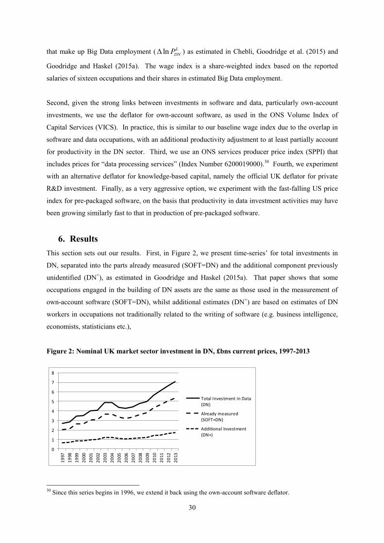
30
that make up Big Data employment ( ln L
DNP ) as estimated in Chebli, Goodridge et al. (2015) and
Goodridge and Haskel (2015a). The wage index is a share-weighted index based on the reported
salaries of sixteen occupations and their shares in estimated Big Data employment.
Second, given the strong links between investments in software and data, particularly own-account
investments, we use the deflator for own-account software, as used in the ONS Volume Index of
Capital Services (VICS). In practice, this is similar to our baseline wage index due to the overlap in
software and data occupations, with an additional productivity adjustment to at least partially account
for productivity in the DN sector. Third, we use an ONS services producer price index (SPPI) that
includes prices for “data processing services” (Index Number 6200019000).30 Fourth, we experiment
with an alternative deflator for knowledge-based capital, namely the official UK deflator for private
R&D investment. Finally, as a very aggressive option, we experiment with the fast-falling US price
index for pre-packaged software, on the basis that productivity in data investment activities may have
been growing similarly fast to that in production of pre-packaged software.
6. Results
This section sets out our results. First, in Figure 2, we present time-series’ for total investments in
DN, separated into the parts already measured (SOFT=DN) and the additional component previously
unidentified (DN+), as estimated in Goodridge and Haskel (2015a). That paper shows that some
occupations engaged in the building of DN assets are the same as those used in the measurement of
own-account software (SOFT=DN), whilst additional estimates (DN+) are based on estimates of DN
workers in occupations not traditionally related to the writing of software (e.g. business intelligence,
economists, statisticians etc.),
Figure 2: Nominal UK market sector investment in DN, £bns current prices, 1997-2013
0
1
2
3
4
5
6
7
8
19
97
19
98
19
99
20
00
20
01
20
02
20
03
20
04
20
05
20
06
20
07
20
08
20
09
20
10
20
11
20
12
20
13
Total Investment in Data
(DN)
Already measured
(SOFT=DN)
Additional Investment
(DN+)
30 Since this series begins in 1996, we extend it back using the own-account software deflator.
31
Note to figure: Solid line is total measured investment in data (DN). Dashed line is the component of investment that we estimate as already measured in official gross fixed capital formation (GFCF) (SOFT=DN). Dotted line is additional investment not already recorded in official GFCF (DN+). Data for the UK market sector, defined as SIC07 sections: A-K, MN, R-U. Source: Goodridge and Haskel (2015a)
To put these estimates into some context, Table 2 presents estimates of nominal investment by asset
over the period 1990 to 2012, including our estimates of investment in data-building and data-based
knowledge creation (DN). A few points to note from Table 2. First, we note the decline in absolute
terms of tangible investment over the late 2000s, as shown in row 6 (compare 2005 and 2012).
Second, we also note the decline in relative terms for certain tangible assets. In particular we note
that, of investment as defined by the SNA,31 the proportion made up by plant & machinery (excluding
IT hardware), row 3, has fallen from 30% in 1990 to 24% in 2012. Similarly, the proportion made up
from investment in vehicles, row 4, has fallen from 11% in 1990 to 4% in 2012. Third, over the same
period, the proportions made up from intangibles has grown. For instance, the share accounted for by
R&D, row 7, has grown from 9% in 1990 to 11% in 2012. That for artistic originals, row 8, has also
grown, from 2% in 1990 to 4% in 2012, whilst that for mineral exploration, row 9, has declined from
2% in 1990 to 1% in 2012. More dramatic is the rise in measured investment in software (memo
item, row 15), which have risen from 9% in 1990 to 19% in 2012.
On investments in data-building and data-based knowledge creation (DN),32 row 12, as set out in
Goodridge and Haskel (2015a), we estimate nominal GFCF to have grown from £1.7bn in 1990 to
£6.6bn in 2012, total growth of 388% implying average annual growth of 18% pa over that period.
In the context of the UK national accounts, our identification of additional investment means that
measured investment in software and databases (see row 15) is actually an underestimate of the
investments made by UK firms. We estimate actual market sector investment in software and
databases of £28.4bn in 2012 (row 13), £1.6bn more than measured in the official data (row 15). In
1990 the difference was just £0.4bn. However, while actual total (row 13) and measured total
investments (row 15) are broadly similar, the implication is that the composition of investment is
31 So including tangibles, plus computerised information (i.e. measured software and databases), mineral exploration, artistic originals and R&D as intangibles, and not including the additional investments in data (DN+) as estimated in Goodridge and Haskel (2015a). 32 References to DN refer to total investments in the D (data-building or transformation) and N (data-based knowledge creation) sectors. Thus D refers to long-lived information assets from the data-building or data transformation process and N refers to long-lived knowledge assets formed from the analysis of information. DN is thus comprised of the part of D and N sector activity already capitalised (SOFT=DN) and the additional part not currently capitalised (DN+).
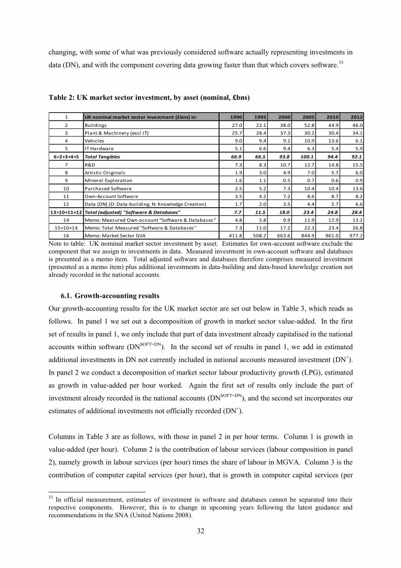
32
changing, with some of what was previously considered software actually representing investments in
data (DN), and with the component covering data growing faster than that which covers software.33
Table 2: UK market sector investment, by asset (nominal, £bns)
1 UK nominal market sector investment (£bns) in: 1990 1995 2000 2005 2010 2012
2 Buildings 27.0 22.1 38.0 52.8 44.9 46.0
3 Plant & Machinery (excl IT) 25.7 28.4 37.3 30.2 30.4 34.1
4 Vehicles 9.0 9.4 9.1 10.9 13.6 6.1
5 IT Hardware 5.1 6.6 9.4 6.3 5.4 5.9
6=2+3+4+5 Total Tangibles 66.9 66.5 93.8 100.1 94.4 92.1
7 R&D 7.3 8.3 10.7 12.7 14.8 15.5
8 Artistic Originals 1.9 3.0 4.9 7.0 5.7 6.0
9 Mineral Exploration 1.6 1.1 0.5 0.7 0.6 0.9
10 Purchased Software 2.5 5.2 7.3 10.4 10.4 13.6
11 Own-Account Software 3.5 4.2 7.2 8.6 8.7 8.2
12 Data [DN] (D: Data-building; N: Knowledge Creation) 1.7 2.0 3.5 4.4 5.7 6.6
13=10+11+12 Total (adjusted) "Software & Databases" 7.7 11.5 18.0 23.4 24.8 28.4
14 Memo: Measured Own-account "Software & Databases" 4.8 5.8 9.9 11.9 12.9 13.2
15=10+14 Memo: Total Measured "Software & Databases" 7.3 11.0 17.2 22.3 23.4 26.8
16 Memo: Market Sector GVA 411.8 508.2 663.6 844.9 961.0 977.2
Note to table: UK nominal market sector investment by asset. Estimates for own-account software exclude the component that we assign to investments in data. Measured investment in own-account software and databases is presented as a memo item. Total adjusted software and databases therefore comprises measured investment (presented as a memo item) plus additional investments in data-building and data-based knowledge creation not already recorded in the national accounts.
6.1. Growth-accounting results
Our growth-accounting results for the UK market sector are set out below in Table 3, which reads as
follows. In panel 1 we set out a decomposition of growth in market sector value-added. In the first
set of results in panel 1, we only include that part of data investment already capitalised in the national
accounts within software (DNSOFT=DN). In the second set of results in panel 1, we add in estimated
additional investments in DN not currently included in national accounts measured investment (DN+).
In panel 2 we conduct a decomposition of market sector labour productivity growth (LPG), estimated
as growth in value-added per hour worked. Again the first set of results only include the part of
investment already recorded in the national accounts (DNSOFT=DN), and the second set incorporates our
estimates of additional investments not officially recorded (DN+).
Columns in Table 3 are as follows, with those in panel 2 in per hour terms. Column 1 is growth in
value-added (per hour). Column 2 is the contribution of labour services (labour composition in panel
2), namely growth in labour services (per hour) times the share of labour in MGVA. Column 3 is the
contribution of computer capital services (per hour), that is growth in computer capital services (per
33 In official measurement, estimates of investment in software and databases cannot be separated into their respective components. However, this is to change in upcoming years following the latest guidance and recommendations in the SNA (United Nations 2008).
33
hour) times the share in MGVA. Column 4 is the contribution of growth in other tangible (buildings,
plant & machinery, vehicles) capital services (per hour). Column 5 is the contribution of growth in
R&D capital services (per hour). Column 6 is the contribution of growth in capital services (per hour)
from mineral exploration and artistic originals. Columns 7 to 11 set out contributions from software
and data-based assets (DN). Column 7 is the contribution of growth in measured software capital
services (per hour). Columns 8 and 9 break the measured software contribution out into two
components. The first, column 8, is an adjusted component for software (SOFT≠DN, adjusted in the
sense that we remove the part of measured investment that we estimate represents investments in
DN). Column 9 shows the contribution from the part of measured investment that we assign to DN
(DNSOFT=DN). Column 10 is the contribution of additional data-based information and knowledge
capital (DN+) not recorded in the national accounts. Column 11 is the total contribution of DN
capital and is the sum of columns 9 and 10. Finally, column 12 is growth in TFP, namely column 1
minus the sum of columns 2 to 7 and column 10.
Consider first the top panel of data for growth in value-added. Growth in value-added was relatively
weak in the early 1990s (1.63% pa) since it includes the recession that took place in that period.
Growth in the late 1990s was much stronger (3.7% pa) before declining in the early 2000s (2.48% pa)
and being only marginally positive in 2005-12 (0.06% pa), the period of the great recession. The
contribution of labour services was negative in the early 1990s, a period where hours worked
declined, grew strongly in the late 1990s, was weaker in the early 2000s and relatively stronger in the
2005-12 period.34 The contribution of computer capital input grew quickly in the late 1990s, but fell
in the 2000s, and more so in the late 2000s so that it stood at just 0.03% pa in 2005-12. For other
tangibles (buildings, plant and vehicles) the decline in the contribution is much less dramatic, partly
due to the much slower depreciation rates for these assets, particularly buildings.
Turning to intangibles, the contribution of R&D rose in the late 1990s, before falling back in the late
2000s, and the contribution of mineral exploration and copyright grew in the late 1990s and again in
the early 2000s, before turning negative in 2005-12 when capital services fell. On measured software,
that contribution rose strongly in the late 1990s (from 0.17% pa to 0.26% pa) and was maintained in
the early 2000s (0.27% pa), following the software investment boom that took place in the late 1990s
and early 2000s, before falling back to a much weaker contribution of 0.05% pa in 2005-12. The
relative weakness of investment in this period combined with the relatively high depreciation rates of
intangible assets has meant that growth in software capital services has been considerably weaker.
34 This is a noted feature of the great recession and the period that has followed. The decline in output growth was not matched by a similar decline in employment or hours worked, and since the recession, hours worked have grown at a similar rate to growth in output, hence discussion of the UK productivity puzzle. For an analysis of the productivity puzzle, please see Goodridge, Haskel et al. (2014b).
34
Implicitly within the measured software contribution are the contributions of software itself
(SOFT≠DN) and measured DN (SOFT=DN) activity, which we break out explicitly in columns 8 and
9. The pattern for software (SOFT≠DN) is similar to that for measured software, although the
contribution is slightly less with the component for DN separated out. On measured DN (DNSOFT=DN),
the estimated contribution is a bit less than that for scientific R&D, at 0.01% pa in the early 1990s,
0.02% pa in the late 1990s and early 2000s and 0.01% pa in 2005-12. Note that this contribution is
already an implicit part of the measured data in the national accounts.
Thus the overall TFP record was one of strong growth in the early 1990s (1.51% pa), falling back in
the late 1990s (1.2% pa) and again in the early 2000s (1.07% pa), and a strong decline in TFP in the
late 2000s (-1.22% pa), largely due to the collapse in TFP during and since the great recession.
In the second set of results in panel 1, we incorporate additional investments in data-based
information and knowledge not already included in the national accounts (DN+), thus increasing the
contribution of DN assets (total contribution of DN in column 11) in the late 1990s, to 0.03% pa, and
in the late 2000s, to 0.02% pa. Thus, as a share of growth in value-added, we estimate that the total
contribution of DN explains 0.8% of ΔlnQ in the 1990s, 0.9% of ΔlnQ in the early 2000s and 22.6%
of ΔlnQ in the late 2000s, with the latter being a period of exceptionally weak growth in output. Note
in column 1 that accounting for these additional investments in DN raises output growth in 2005-12
from 0.06% pa in the first set of results to 0.07% pa in the second set.
Note also that, in particular when we fully account for all investments in DN, the contribution of data-
based information and knowledge is comparable to that of R&D. Although this obviously does not
consider the role of spillovers, which R&D is widely considered to generate (see e.g. Hall, Mairesse et
al. (2009) for a survey), given the attention devoted to R&D this is clearly a significant finding.
Results in panel 2 present a similar exercise but this time using a decomposition of LPG so that
estimated contributions are all in per hour terms. Again the first set of results only include measured
national accounts investments in DN (DNSOFT=DN), and the second set incorporates additional
investments (DN+). From column 1 we see that LPG has been on a downward trajectory since the
early 1990s, estimated at 3.12% pa in 1990-95, 2.73% pa in 1995-00, 2.46% in 2000-05 and just
0.10% pa in 2005-12. In column 2 we see that the contribution of labour composition rose in the late
1990s, declined in the early 2000s before rising to a very high contribution of 0.56% pa in the 2005-
12 period. As noted in Franklin and Mistry (2013), labour composition has improved quite
dramatically since the recession, with firms upskilling, that is increasing the hours of their more
skilled and/or experienced workers, and reducing the hours of the less skilled/experienced. In
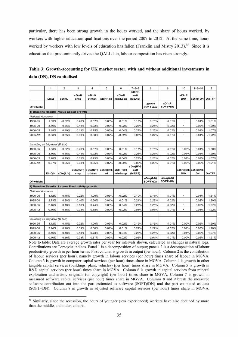
35
particular, there has been strong growth in the hours worked, and the share of hours worked, by
workers with higher education qualifications over the period 2007 to 2012. At the same time, hours
worked by workers with low levels of education has fallen (Franklin and Mistry 2013).35 Since it is
education that predominantly drives the QALI data, labour composition has risen strongly.
Table 3: Growth-accounting for UK market sector, with and without additional investments in
data (DN), DN capitalised
1 2 3 4 5 6 7=8+9 8 9 10 11=9+10 12
DlnQ sDlnL
sDlnK
cmp
sDlnK
othtan sDlnR rd
sDlnR
min&cop
sDlnR
soft
(MEAS)
sDlnR
DN+ sDlnR DN DlnTFP
Of which:
sDlnR
SOFT ≠DN
sDlnR
SOFT=DN
National Accounts
1990-95 1.63% -0.82% 0.20% 0.57% 0.00% 0.01% 0.17% 0.16% 0.01% - 0.01% 1.51%
1995-00 3.70% 0.86% 0.41% 0.92% 0.03% 0.02% 0.26% 0.24% 0.02% - 0.02% 1.20%
2000-05 2.48% 0.19% 0.13% 0.75% 0.03% 0.04% 0.27% 0.25% 0.02% - 0.02% 1.07%
2005-12 0.06% 0.55% 0.03% 0.66% 0.02% -0.02% 0.05% 0.04% 0.01% - 0.01% -1.22%
Including all 'big data' (D & N)
1990-95 1.63% -0.82% 0.20% 0.57% 0.00% 0.01% 0.17% 0.16% 0.01% 0.00% 0.01% 1.50%
1995-00 3.70% 0.86% 0.41% 0.92% 0.03% 0.02% 0.26% 0.24% 0.02% 0.01% 0.03% 1.20%
2000-05 2.48% 0.19% 0.13% 0.75% 0.03% 0.04% 0.27% 0.25% 0.02% 0.01% 0.02% 1.07%
2005-12 0.07% 0.55% 0.03% 0.65% 0.02% -0.02% 0.05% 0.03% 0.01% 0.00% 0.02% -1.21%
DlnQ/H sDln(L/H)
sDln(K/H)
cmp
sDln(K/H)
othtan
sDln(R/H)
rd
sDln(R/H)
min&cop
sDln(R/H)
soft
(MEAS)
sDln(R/H)
DN+
sDln(R/H)
DN DlnTFP
Of which:
sDln(R/H)
SOFT ≠DN
sDln(R/H)
SOFT=DN
National Accounts
1990-95 3.12% 0.15% 0.22% 1.00% 0.03% 0.02% 0.19% 0.18% 0.01% - 0.01% 1.51%
1995-00 2.73% 0.28% 0.40% 0.60% 0.01% 0.01% 0.24% 0.22% 0.02% - 0.02% 1.20%
2000-05 2.46% 0.18% 0.13% 0.74% 0.03% 0.04% 0.27% 0.25% 0.02% - 0.02% 1.07%
2005-12 0.10% 0.56% 0.03% 0.68% 0.02% -0.02% 0.05% 0.04% 0.01% - 0.01% -1.22%
Including all 'big data' (D & N)
1990-95 3.12% 0.15% 0.22% 1.00% 0.03% 0.02% 0.19% 0.18% 0.01% 0.00% 0.02% 1.50%
1995-00 2.74% 0.28% 0.39% 0.60% 0.01% 0.01% 0.24% 0.22% 0.02% 0.01% 0.03% 1.20%
2000-05 2.46% 0.18% 0.13% 0.73% 0.03% 0.04% 0.26% 0.25% 0.02% 0.01% 0.02% 1.07%
2005-12 0.10% 0.56% 0.03% 0.67% 0.02% -0.02% 0.05% 0.04% 0.01% 0.00% 0.02% -1.21%
1) Baseline Results: Value-added growth
2) Baseline Results: Labour Productivity growth
Note to table: Data are average growth rates per year for intervals shown, calculated as changes in natural logs. Contributions are Tornqvist indices. Panel 1 is a decomposition of output; panels 2 is a decomposition of labour productivity growth in per hour terms. First column is growth in output (per hour). Column 2 is the contribution of labour services (per hour), namely growth in labour services (per hour) times share of labour in MGVA. Column 3 is growth in computer capital services (per hour) times share in MGVA. Column 4 is growth in other tangible capital services (buildings, plant, vehicles) (per hour) times share in MGVA. Column 5 is growth in R&D capital services (per hour) times share in MGVA. Column 6 is growth in capital services from mineral exploration and artistic originals (or copyright) (per hour) times share in MGVA. Column 7 is growth in measured software capital services (per hour) times share in MGVA. Columns 8 and 9 break the measured software contribution out into the part estimated as software (SOFT≠DN) and the part estimated as data (SOFT=DN). Column 8 is growth in adjusted software capital services (per hour) times share in MGVA,
35 Similarly, since the recession, the hours of younger (less experienced) workers have also declined by more than the middle, and older, cohorts.
36
adjusted in the sense that the part assigned to data has been removed. Column 9 is growth in measured data (SOFT=DN) capital services (per hour) times share in MGVA. Column 10 is growth in additional data (DN+) capital services (per hour) times share in MGVA. In each of panels 1 and 2, the first set of results only include measured data investment, thus column 10 is blank, and the second set incorporate additional investments not recorded in the national accounts. Column 11 is the total contribution of DN capital services and is thus column 9 plus column 10. Column 12 is TFP, namely column 1 minus the sum of columns 2 to 7 minus column 10. Contributions may not sum exactly due to rounding.
In columns 3 to 11 we present the contributions from capital deepening (i.e. capital services per hour)
for our various assets and some aggregations. The pattern here is broadly similar to that in the
decomposition of value-added, including for DN assets. Using the national accounts model in the top
half of panel 2, the estimated contribution for DNSOFT=DN capital deepening (column 9) rose in the late
1990s and was maintained in the early 2000s before falling back in the late 2000s. Once we
incorporate additional investments, DN+, as in the lower half of panel 2, we find that the total
contribution (column 11) is higher, rising from 0.02% pa in 1990-95, to 0.03% pa in 1995-00, and
then remaining at 0.02% pa throughout the 2000s. Thus we find that once we account for all
investments in DN, as a share of Δln(Q/H), the contribution of DN capital deepening can explain 0.6%
of labour productivity growth in the early 1990s, 1% in the late 1990s, 0.9% in the early 2000s, and
15.1% in the late 2000s, when LPG was very weak.
6.2. Growth-accounting: further details and robustness checks
So far our main findings are that, first, the contribution of data-based information and knowledge
(DN) is comparable to that of R&D, and second, most of that contribution is already measured as an
implicit part of the official data on software. We necessarily make a number of assumptions when
implementing the growth accounting exercise. How robust are our findings to key assumptions? This
is shown in Table 4.
Table 4 is set out as follows. Data are averages for 2005-12. Row 1 is growth in market sector value-
added with DN fully capitalised. Row 2 is the measured software contribution. Rows 3 and 4 break
row 2 out into the contribution of software (SOFT≠DN) and the contribution of DN already implicit
in the measured data (SOFT=DN). Row 5 is the contribution of additional investments in DN not
already measured in official data (DN+). Row 6 is the total contribution of DN assets and so is the
sum of rows 5 and 4. Finally row 7 is the total contribution of software and databases and is thus the
sum of rows 2 and 5, or alternatively the sum of rows 3 and 6. In each column we test the robustness
of these terms to various assumptions on the depreciation rate and DN price index. Column 1 are our
baseline estimates, based on a depreciation rate of 0.33 and using a share-weighted wage index for
DN workers (see Goodridge and Haskel (2015a) for more details) as the deflator. In columns 2 and 3
we halve and double the depreciation rate respectively. In column 4, we revert to a depreciation rate
of 0.33, but use the own-account software price index to deflate DN investment, note this price index
37
includes an adjustment to account for productivity growth in asset production. In column 5 we deflate
using the ONS SPPI for ‘Data processing’ services. In column 6 we use the UK R&D deflator.
Finally in column 7, we use the US pre-packaged software deflator, implicitly assuming very fast
productivity growth in production of DN assets.
Let us first consider the depreciation rate. In column 1 we apply the same depreciation rate as
commonly used for software, based on the strong links between investments in DN and software in
both concept and measurement practice, as outlined in Goodridge and Haskel (2015a) and this paper,
namely a rate of 0.33.36 In column 2 we halve that rate to 0.167. The impact on the estimated
contribution (row 6) is however small – with rounding, there are no changes to the estimated
contributions. In column 3 we double the depreciation rate to 0.67. The impact is to increase the
contribution of DN assets.37 The contribution of SOFT=DN (row 4) is raised from 0.01% pa to 0.02%
pa and that from DN+ (row 5) is raised from 0.00% pa to 0.01% pa. However, with rounding, the total
contribution of DN (row 6) remains at 0.02% pa.
In the remaining columns we test the robustness of our assumptions on the price of DN assets. Whilst
a great deal has been done to improve estimates of investment in knowledge assets, including in
official national accounting, less has been done on estimation of their prices. Such estimation is
difficult as a feature of these assets is that they are rarely acquired via market transactions. Indeed
one of the benefits of ownership is the sole right or access to knowledge unavailable to market
competitors. Therefore much investment takes place in-house, and no market price can be recorded.
For this reason, in much academic work the standard approach has been to use an implied value-added
or GDP deflator, implicitly assuming that knowledge prices closely follow a weighted average of
prices in the rest of the economy. An alternative, often used in national accounting, is to use an input
price index based on the inputs to asset production. For instance, in the case of own-account
software, the ONS deflate investment using a wage index of the salaries of software-related
occupations and an assumed adjustment for productivity based on LPG in the wider service sector. In
the case of R&D, the UK price index is a share-weighted index based on the price of labour and
intermediate inputs to R&D and their share in R&D investment, with no adjustment for productivity.
36 Assuming a double-declining balance rate where δ=2/T, a rate of depreciation of 0.33 implies a life-length for data-based information and knowledge of 6 years. This should be considered as an average across all DN assets. Some DN assets will have longer service lives and others shorter. Halving and doubling the depreciation rate implies average life-lengths of 12 years and 3 years respectively. 37 This seems somewhat counter-intuitive. It might be expected that increasing the depreciation rate would reduce the contribution of DN assets. However, raising the depreciation rate also lowers the level of the DN capital stock in earlier years such that the growth rate is raised in later years, thus in this case raising the contribution.
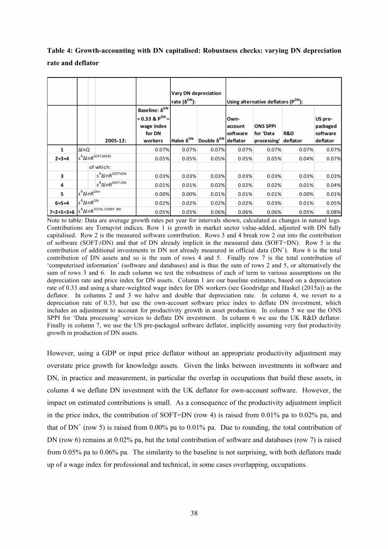
38
Table 4: Growth-accounting with DN capitalised: Robustness checks: varying DN depreciation
rate and deflator
Note to table: Data are average growth rates per year for intervals shown, calculated as changes in natural logs. Contributions are Tornqvist indices. Row 1 is growth in market sector value-added, adjusted with DN fully capitalised. Row 2 is the measured software contribution. Rows 3 and 4 break row 2 out into the contribution of software (SOFT≠DN) and that of DN already implicit in the measured data (SOFT=DN). Row 5 is the contribution of additional investments in DN not already measured in official data (DN+). Row 6 is the total contribution of DN assets and so is the sum of rows 4 and 5. Finally row 7 is the total contribution of ‘computerised information’ (software and databases) and is thus the sum of rows 2 and 5, or alternatively the sum of rows 3 and 6. In each column we test the robustness of each of term to various assumptions on the depreciation rate and price index for DN assets. Column 1 are our baseline estimates, based on a depreciation rate of 0.33 and using a share-weighted wage index for DN workers (see Goodridge and Haskel (2015a)) as the deflator. In columns 2 and 3 we halve and double that depreciation rate. In column 4, we revert to a depreciation rate of 0.33, but use the own-account software price index to deflate DN investment, which includes an adjustment to account for productivity growth in asset production. In column 5 we use the ONS SPPI for ‘Data processing’ services to deflate DN investment. In column 6 we use the UK R&D deflator. Finally in column 7, we use the US pre-packaged software deflator, implicitly assuming very fast productivity growth in production of DN assets.
However, using a GDP or input price deflator without an appropriate productivity adjustment may
overstate price growth for knowledge assets. Given the links between investments in software and
DN, in practice and measurement, in particular the overlap in occupations that build these assets, in
column 4 we deflate DN investment with the UK deflator for own-account software. However, the
impact on estimated contributions is small. As a consequence of the productivity adjustment implicit
in the price index, the contribution of SOFT=DN (row 4) is raised from 0.01% pa to 0.02% pa, and
that of DN+ (row 5) is raised from 0.00% pa to 0.01% pa. Due to rounding, the total contribution of
DN (row 6) remains at 0.02% pa, but the total contribution of software and databases (row 7) is raised
from 0.05% pa to 0.06% pa. The similarity to the baseline is not surprising, with both deflators made
up of a wage index for professional and technical, in some cases overlapping, occupations.
2005-12:
Baseline: δDN
= 0.33 & PDN
=
wage index
for DN
workers Halve δDN Double δDN
Own-
account
software
deflator
ONS SPPI
for 'Data
processing'
R&D
deflator
US pre-
packaged
software
deflator
1 ΔlnQ 0.07% 0.07% 0.07% 0.07% 0.07% 0.07% 0.07%
2=3+4 sRΔlnRSOFT,MEAS
0.05% 0.05% 0.05% 0.05% 0.05% 0.04% 0.07%
of which:
3 sRΔlnRSOFT≠DN 0.03% 0.03% 0.03% 0.03% 0.03% 0.03% 0.03%
4 sRΔlnRSOFT=DN
0.01% 0.01% 0.02% 0.02% 0.02% 0.01% 0.04%
5 sRΔlnRDN+
0.00% 0.00% 0.01% 0.01% 0.01% 0.00% 0.01%
6=5+4 sRΔlnRDN
0.02% 0.02% 0.02% 0.02% 0.03% 0.01% 0.05%
7=2+5=3+6 sRΔlnRTOTAL COMP. INF.
0.05% 0.05% 0.06% 0.06% 0.06% 0.05% 0.08%
Vary DN depreciation
rate (δDN): Using alternative deflators (P
DN):
39
As discussed, there are two aspects to DN investment that we have sought to measure. The first is
investment in the data-building (D) stage, which captures the resources devoted to the transformation
of raw records into analysable information. Therefore in column 5 we apply the ONS SPPI for data
processing services. Relative to the baseline, the contribution of SOFT=DN (row 4) is raised from
0.01% pa to 0.02% pa and that of DN+ (row 5) is raised from 0.00% pa to 0.01% pa. Thus the total
contribution of DN (row 6) is raised from 0.02% pa to 0.03% pa, and the total contribution of
software and databases (row 7) is raised from 0.05% pa to 0.06% pa.
The second aspect of DN investment is the resources devoted to the extraction of knowledge (N) from
data/information. Therefore in column 6 we apply a price index designed to measure the price of
extracting knowledge from R&D. Relative to the baseline, the contributions of SOFT=DN (row 4)
and DN+ (row 5) are unchanged, but due to rounding, the total contribution of DN (row 6) is reduced
from 0.02% pa to 0.01% pa. The total contribution of software and databases (row 7) is unchanged.
Finally in column 7, we use the US BEA deflator for pre-packaged software. This is by far the most
aggressive of all the alternatives presented in Table 4. The index falls at a rate of around -5% pa over
the period 1990 to 2012, reflecting strong growth in the quality of pre-packaged software and
implying strong productivity growth in their production. Therefore, in applying this index we
speculate on the contribution of DN if productivity growth in the upstream DN sectors is comparable
to that in the production of pre-packaged software. Relative to the baseline, the contribution of
SOFT=DN (row 4) is raised four-fold, from 0.01% pa to 0.04% pa. The contribution of DN+ (row 5)
is raised from 0.00% pa to 0.01% pa. Thus the total contribution of DN (row 6) is more than doubled,
from 0.02% pa to 0.05% pa, and the total contribution of software and databases (row 7) is raised
from 0.05% pa to 0.08% pa.
Overall we conclude that our results are fairly robust to various assumptions on depreciation and
prices, unless one takes the view that productivity growth in data-based asset creation has been
particularly strong, as in the production of pre-packaged software. In that case the estimated
contribution is more than double that in our baseline results. Full growth-accounting results, based on
a decomposition of LPG, using each of the alternative deflators, are presented in Appendix Table A2.
6.3. The contribution of Big Data to measured output growth
The above data were constructed with DN fully capitalised in output (Q). In equation (13) we set out
how DN affects measured growth (ΔlnQM), including the various biases if DN is not fully capitalised.
Thus in Table 5 we show the impact of Big Data on ΔlnQM (column 1). As set out in (13), the effect
of DN on ΔlnQM depends on the overall income share for intangibles (R
Qs , column 2), the shares for
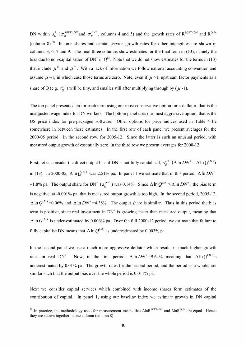
40
DN within R
Qs (SOFT DN
R and
DN
R , columns 4 and 5) and the growth rates of RSOFT=DN and RDN+
(column 8).38 Income shares and capital service growth rates for other intangibles are shown in
columns 3, 6, 7 and 9. The final three columns show estimates for the final term in (13), namely the
bias due to non-capitalisation of DN+ in QM. Note that we do not show estimates for the terms in (13)
that include D and
N . With a lack of information we follow national accounting convention and
assume =1, in which case those terms are zero. Note, even if >1, upstream factor payments as a
share of Q (e.g. DL
Qs ) will be tiny, and smaller still after multiplying through by ( -1).
The top panel presents data for each term using our most conservative option for a deflator, that is the
unadjusted wage index for DN workers. The bottom panel uses our most aggressive option, that is the
US price index for pre-packaged software. Other options for price indices used in Table 4 lie
somewhere in between these estimates. In the first row of each panel we present averages for the
2000-05 period. In the second row, for 2005-12. Since the latter is such an unusual period, with
measured output growth of essentially zero, in the third row we present averages for 2000-12.
First, let us consider the direct output bias if DN is not fully capitalised, ( )( ln ln )DN M
Qs DN Q
in (13). In 2000-05, ( )ln MQ was 2.51% pa. In panel 1 we estimate that in this period, ln DN
=1.8% pa. The output share for DN+ (DN
Qs
) was 0.14%. Since ( )ln MQ > ln DN , the bias term
is negative, at -0.001% pa, that is measured output growth is too high. In the second period, 2005-12,
( )ln MQ =0.06% and ln DN =4.38%. The output share is similar. Thus in this period the bias
term is positive, since real investment in DN+ is growing faster than measured output, meaning that
( )ln MQ is under-estimated by 0.006% pa. Over the full 2000-12 period, we estimate that failure to
fully capitalise DN means that ( )ln MQ is underestimated by 0.003% pa.
In the second panel we use a much more aggressive deflator which results in much higher growth
rates in real DN+. Now, in the first period, ln DN =9.64% meaning that ( )ln MQ is
underestimated by 0.01% pa. The growth rates for the second period, and the period as a whole, are
similar such that the output bias over the whole period is 0.011% pa.
Next we consider capital services which combined with income shares form estimates of the
contribution of capital. In panel 1, using our baseline index we estimate growth in DN capital
38 In practice, the methodology used for measurement means that ΔlnRSOFT=DN and ΔlnRDN+ are equal. Hence
they are shown together in one column (column 8).
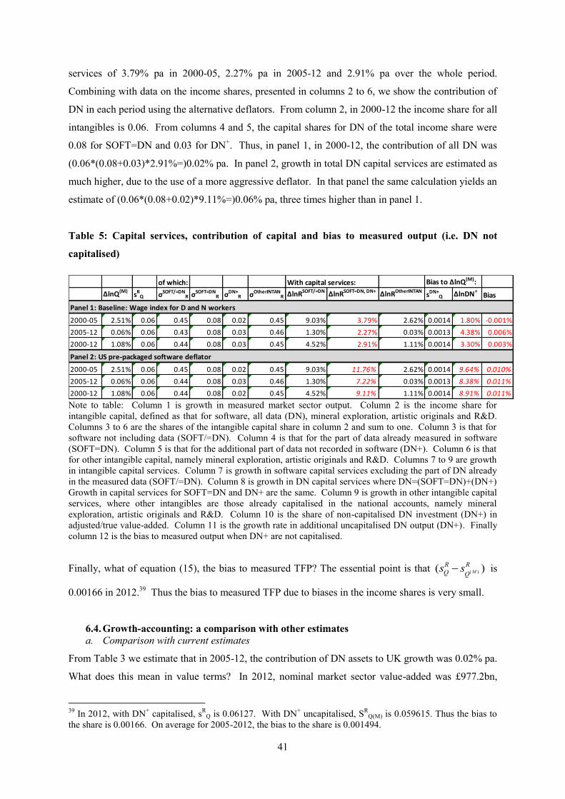
41
services of 3.79% pa in 2000-05, 2.27% pa in 2005-12 and 2.91% pa over the whole period.
Combining with data on the income shares, presented in columns 2 to 6, we show the contribution of
DN in each period using the alternative deflators. From column 2, in 2000-12 the income share for all
intangibles is 0.06. From columns 4 and 5, the capital shares for DN of the total income share were
0.08 for SOFT=DN and 0.03 for DN+. Thus, in panel 1, in 2000-12, the contribution of all DN was
(0.06*(0.08+0.03)*2.91%=)0.02% pa. In panel 2, growth in total DN capital services are estimated as
much higher, due to the use of a more aggressive deflator. In that panel the same calculation yields an
estimate of (0.06*(0.08+0.02)*9.11%=)0.06% pa, three times higher than in panel 1.
Table 5: Capital services, contribution of capital and bias to measured output (i.e. DN not
capitalised)
Note to table: Column 1 is growth in measured market sector output. Column 2 is the income share for intangible capital, defined as that for software, all data (DN), mineral exploration, artistic originals and R&D. Columns 3 to 6 are the shares of the intangible capital share in column 2 and sum to one. Column 3 is that for software not including data (SOFT/=DN). Column 4 is that for the part of data already measured in software (SOFT=DN). Column 5 is that for the additional part of data not recorded in software (DN+). Column 6 is that for other intangible capital, namely mineral exploration, artistic originals and R&D. Columns 7 to 9 are growth in intangible capital services. Column 7 is growth in software capital services excluding the part of DN already in the measured data (SOFT/=DN). Column 8 is growth in DN capital services where DN=(SOFT=DN)+(DN+) Growth in capital services for SOFT=DN and DN+ are the same. Column 9 is growth in other intangible capital services, where other intangibles are those already capitalised in the national accounts, namely mineral exploration, artistic originals and R&D. Column 10 is the share of non-capitalised DN investment (DN+) in adjusted/true value-added. Column 11 is the growth rate in additional uncapitalised DN output (DN+). Finally column 12 is the bias to measured output when DN+ are not capitalised.
Finally, what of equation (15), the bias to measured TFP? The essential point is that ( )( )M
R R
Q Qs s is
0.00166 in 2012.39 Thus the bias to measured TFP due to biases in the income shares is very small.
6.4. Growth-accounting: a comparison with other estimates
a. Comparison with current estimates
From Table 3 we estimate that in 2005-12, the contribution of DN assets to UK growth was 0.02% pa.
What does this mean in value terms? In 2012, nominal market sector value-added was £977.2bn,
39 In 2012, with DN+ capitalised, sR
Q is 0.06127. With DN+ uncapitalised, SRQ(M) is 0.059615. Thus the bias to
the share is 0.00166. On average for 2005-2012, the bias to the share is 0.001494.
of which: With capital services: Bias to ΔlnQ(M):
ΔlnQ(M)s
RQ σSOFT/=DN
R σSOFT=DNR σDN+
R σOtherINTANR ΔlnRSOFT/=DN ΔlnRSOFT=DN, DN+ ΔlnROtherINTAN
sDN+
Q ΔlnDN+Bias
2000-05 2.51% 0.06 0.45 0.08 0.02 0.45 9.03% 3.79% 2.62% 0.0014 1.80% -0.001%
2005-12 0.06% 0.06 0.43 0.08 0.03 0.46 1.30% 2.27% 0.03% 0.0013 4.38% 0.006%
2000-12 1.08% 0.06 0.44 0.08 0.03 0.45 4.52% 2.91% 1.11% 0.0014 3.30% 0.003%
2000-05 2.51% 0.06 0.45 0.08 0.02 0.45 9.03% 11.76% 2.62% 0.0014 9.64% 0.010%
2005-12 0.06% 0.06 0.44 0.08 0.03 0.46 1.30% 7.22% 0.03% 0.0013 8.38% 0.011%
2000-12 1.08% 0.06 0.44 0.08 0.02 0.45 4.52% 9.11% 1.11% 0.0014 8.91% 0.011%
Panel 1: Baseline: Wage index for D and N workers
Panel 2: US pre-packaged software deflator
42
implying that the flow of DN capital services contributed a value of around
((0.0155/100)*977.2=)£0.152bn or £152m to UK market sector growth 2012.40 How does this
compare to other results in the literature? Estimates of the contribution of Big Data to the UK
economy are uncommon. However, CEBR (2012) estimate that in 2011, the aggregate economic
benefits derived from Big Data were £25.1bn pa.41 Performing a similar calculation to above suggests
that, according to CEBR, the contribution of Big Data was around (25.1/975.7=)2.57% pa,
considerably more than actual growth in value-added (1.49% pa) in that year. Therefore, whilst the
contribution of data-based information and knowledge might grow in the coming years, the results
reported in this paper suggest that some statements made on the current and potential future
contribution of data and data analytics seem very much like overstatements of reality.
The reason for why estimates such as those in CEBR (2012) are unrealistic, is that the income share
for data is relatively small. At just 0.007 it is a third of that for R&D and a quarter of that for
software. Therefore in 2000-12, whilst growth in DN capital services at 2.27% pa is higher than those
from R&D (1.11% pa), software (1.30% pa), plant & machinery (1.38% pa) and indeed all assets in
total (2.03% pa), the contribution is small. (Data on income shares, capital services and contributions
by asset are presented in Appendix Table A3).
b. Future projections
Data transformation and data analytics are growing activities so we would expect higher growth in
capital services in future. The higher stock will also mean a higher income share for data which will
also act to raise the estimated contribution. So what might we expect the future contribution to be? In
the following chart we compare the DN income share with that for (adjusted) software. In 2012, the
DN income stood at 0.71%, similar to that for software in the mid-1980s. However, as investment in
software continued, growth in the software capital stock meant that the income share grew
considerably, peaking at 3% following the software investment boom of the late 1990s and early
2000s, and settling at around 2.6% in recent years. Just as with software in the 1970s and 1980s, Big
Data is an emerging and growing field. If we assume a similar pattern for DN, then a gradually
growing income share will raise the estimated contribution of data in the coming years and decades.
40 This calculation is based on an estimate for UK market sector value-added. A similar calculation on the basis of whole economy GDP (at basic prices) would yield an estimate of ((0.0155/100)*1593.9=)£0.247bn or £247m. Note, this implicitly assumes that the returns from, and the contribution of, DN in the non-market sector is the same or similar to those in the market sector. 41 CEBR (2012) define aggregate economic benefits as the sum of estimated benefits from “business efficiency, business innovation and business creation”
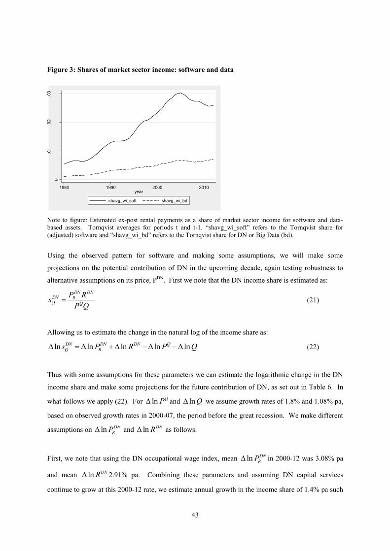
43
Figure 3: Shares of market sector income: software and data
Note to figure: Estimated ex-post rental payments as a share of market sector income for software and data-based assets. Tornqvist averages for periods t and t-1. “shavg_wi_soft” refers to the Tornqvist share for (adjusted) software and “shavg_wi_bd” refers to the Tornqvist share for DN or Big Data (bd).
Using the observed pattern for software and making some assumptions, we will make some
projections on the potential contribution of DN in the upcoming decade, again testing robustness to
alternative assumptions on its price, PDN. First we note that the DN income share is estimated as:
DN DNDN RQ Q
P Rs
P Q (21)
Allowing us to estimate the change in the natural log of the income share as:
ln ln ln ln lnDN DN DN Q
Q Rs P R P Q (22)
Thus with some assumptions for these parameters we can estimate the logarithmic change in the DN
income share and make some projections for the future contribution of DN, as set out in Table 6. In
what follows we apply (22). For ln QP and lnQ we assume growth rates of 1.8% and 1.08% pa,
based on observed growth rates in 2000-07, the period before the great recession. We make different
assumptions on ln DN
RP and ln DNR as follows.
First, we note that using the DN occupational wage index, mean ln DN
RP in 2000-12 was 3.08% pa
and mean ln DNR 2.91% pa. Combining these parameters and assuming DN capital services
continue to grow at this 2000-12 rate, we estimate annual growth in the income share of 1.4% pa such
0
.01
.02
.03
1980 1990 2000 2010year
shavg_wi_soft shavg_wi_bd
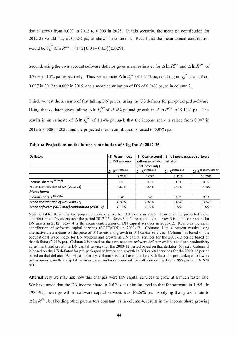
44
that it grows from 0.007 in 2012 to 0.009 in 2025. In this scenario, the mean pa contribution for
2012-25 would stay at 0.02% pa, as shown in column 1. Recall that the mean annual contribution
would be ln 1/ 2 0.01 0.05 0.0291DN DNQs R .
Second, using the own-account software deflator gives mean estimates for ln DN
RP and ln DNR of
0.79% and 5% pa respectively. Thus we estimate ln DN
Qs of 1.21% pa, resulting in DN
Qs rising from
0.007 in 2012 to 0.009 in 2015, and a mean contribution of DN of 0.04% pa, as in column 2.
Third, we test the scenario of fast falling DN prices, using the US deflator for pre-packaged software.
Using that deflator gives falling ln DN
RP of -3.4% pa and growth in ln DNR of 9.11% pa. This
results in an estimate of ln DN
Qs of 1.14% pa, such that the income share is raised from 0.007 in
2012 to 0.008 in 2025, and the projected mean contribution is raised to 0.07% pa.
Table 6: Projections on the future contribution of ‘Big Data’: 2012-25
Note to table: Row 1 is the projected income share for DN assets in 2025. Row 2 is the projected mean contribution of DN assets over the period 2012-25. Rows 3 to 5 are memo items. Row 3 is the income share for DN assets in 2012. Row 4 is the mean contribution of DN capital services in 2000-12. Row 5 is the mean contribution of software capital services (SOFT≠DN) in 2000-12. Columns 1 to 4 present results using alternative assumptions on the price of DN assets and growth in DN capital services. Column 1 is based on the occupational wage index for DN workers and growth in DN capital services for the 2000-12 period based on that deflator (2.91% pa). Column 2 is based on the own-account software deflator which includes a productivity adjustment, and growth in DN capital services for the 2000-12 period based on that deflator (5% pa). Column 3 is based on the US deflator for pre-packaged software and growth in DN capital services for the 2000-12 period based on that deflator (9.11% pa). Finally, column 4 is also based on the US deflator for pre-packaged software but assumes growth in capital services based on those observed for software on the 1985-1995 period (16.26% pa).
Alternatively we may ask how this changes were DN capital services to grow at a much faster rate.
We have noted that the DN income share in 2012 is at a similar level to that for software in 1985. In
1985-95, mean growth in software capital services was 16.26% pa. Applying that growth rate to
ln DNR , but holding other parameters constant, as in column 4, results in the income share growing
Deflator: (1): Wage index
for DN workers
(2): Own-account
software deflator
(incl. prod. adj.)
ΔlnRDN (2000-12) ΔlnRDN (2000-12) ΔlnRDN (2000-12) ΔlnRDN (SOFT, 1985-95)
2.91% 5.00% 9.11% 16.26%
Income share: sDN (2025)
0.01 0.01 0.01 0.02
Mean contribution of DN (2012-25) 0.02% 0.04% 0.07% 0.23%
Memo items:
Income share: sDN (2012)
0.01 0.01 0.01 0.01
Mean contribution of DN (2000-12) 0.02% 0.03% 0.06% 0.06%
Mean software (SOFT ≠DN) contribution (2000-12) 0.12% 0.12% 0.12% 0.12%
(3): US pre-packaged software
deflator
45
to 0.02. Thus the projection for the average contribution of DN is 0.23% pa, a large contribution
around twice as high as software in the 2000-12 period. We note however that a ln DNR of 16.26%
would require significantly higher growth rates in nominal DN investment.
Thus Table 6 shows that projections on the future contribution of DN crucially depend on what
happens to prices, and therefore ultimately, the path of upstream TFP. Results in column 3 and 4 are
based on the assumption of fast-falling prices for DN, or put another way, high TFP in DN
production. If this is the case, the contribution of DN may rise strongly. Alternatively, if prices do
not fall but instead grow moderately, as in columns 1 to 2, a large growth in the contribution will
require extremely high growth in nominal DN investment. Therefore we settle on a central projected
contribution of 0.04% to 0.07% pa over the coming decade, slightly higher than the typical
contribution from R&D.
7. Conclusions
This paper has set out an economic framework for the measurement of activity in Big Data (and Big
Data analytics) embedded in national accounting and growth-accounting frameworks in a consistent
way to eliminate double-counting. In it we define data, information, ideas and knowledge. As part of
our framework, we show how some investments in data are already measured in GDP, but some are
missed. In implementing our framework we apply the official methodology for estimating investment
in software, that is by identifying occupations engaged in asset production. The implication of this is
at least some part of investments in Big Data activity are already counted in the measurement of
software. Our findings are as follows. First, we estimate total investment in data-based information
and knowledge as £6.6bn in 2012. Second, of that £6.6bn, £5bn is already counted in the
measurement of software. Thus capitalisation adds £1.6bn to measured GDP. Third, incorporating
those measures into a growth-accounting framework, we estimate that in 2005 to 2012, data-based
information and knowledge contributed 0.02% pa of growth in UK market sector value-added, which
in value terms translates to around £152m. We therefore regard other estimates in the literature, such
as those in CEBR (2012), that Big Data is currently adding in the order of £25bn of annual benefits to
the UK economy as over-estimates, although we do expect the contribution of data-based assets to
grow in coming years. Finally, we use various parameters from our framework to form some
projections on the likely contribution of Big Data over the upcoming decade, forming a central
estimate of a mean contribution of around 0.07% to 0.23% pa in the period 2012-25, with the lower
bound of this range being slightly higher than the typical contribution from R&D.
46
References
Abramovitz, M. (1956). Resource and output trends in the United States since 1870, NBER. Arrow, K. J. (1984). The economics of information, Harvard University Press. Bakhshi, H., A. Bravo-Biosca, et al. (2014). Inside the Datavores: Estimating the effect of data and
online analytics on firm performance. Basu, S., J. G. Fernald, et al. (2001). Productivity growth in the 1990s: technology, utilization, or
adjustment? Carnegie-Rochester conference series on public policy, Elsevier. Bertino, E., P. Bernstein, et al. (2011). "Challenges and Opportunities with Big Data." Boisot, M. and A. Canals (2004). "Data, information and knowledge: have we got it right?" Journal of
Evolutionary Economics 14(1): 43-67. Borgo, M. D., P. Goodridge, et al. (2013). "Productivity and Growth in UK Industries: An Intangible
Investment Approach*." Oxford Bulletin of Economics and Statistics 75(6): 806-834. Brynjolfsson, E., L. Hitt, et al. (2011). "Strength in Numbers: How Does Data-Driven
Decisionmaking Affect Firm Performance?" Available at SSRN 1819486. CEBR (2012). "Data Equity. Unlocking the value of big data." Report for SAS April 2012. CEBR (2013). "Data on the Balance Sheet: Report for SAS, June 2013." Chamberlin, G., T. Clayton, et al. (2007). "New measures of UK private sector software investment."
Economic and Labour Market Review 1(5): 17-28. Chebli, O., P. Goodridge, et al. (2015). "Measuring activity in Big Data: New estimates of Big Data
employment in the UK market sector." Copeland, A. M., G. W. Medeiros, et al. (2007). "Estimating Prices for R&D Investment in the 2007
R&D Satellite Account." BEA Papers. Corrado, C., P. Goodridge, et al. (2011). "Constructing a Price Deflator for R&D: Calculating the
Price of Knowledge Investments as a Residual." Corrado, C., C. Hulten, et al. (2005). Measuring capital and technology: an expanded framework. C.
Hulten, University of Chicago Press. Davenport, T. H. and J. G. Harris (2007). Competing on analytics: the new science of winning,
Harvard Business Press. e-skills UK (2013b). "Big Data Analytics: Adoption and Employment Trends, 2012-2017." Economist Intelligence Unit (2012). "The Deciding Factor: Big Data & Decision Making." Capgemini
Reports: 1-24. Franklin, M. and P. Mistry (2013). "Quality-adjusted labour input: estimates to 2011 and First
Estimates to 2012." ONS, available at http://www. ons. gov. uk/ons/dcp171766_317119. pdf. Fransman, M. (1998). "Information, knowledge, vision and theories of the firm." Technology,
organization, and competitiveness: perspectives on industrial and corporate change: 147-191. Goodridge, P. (2014). "Film, Television & Radio, Books, Music and Art: Estimating UK Investment
in Artistic Originals." Imperial College Discussion Paper 2014/2(March 2014). Goodridge, P. and J. Haskel (2015a). "How much is UK business investing in Big Data." Goodridge, P., J. Haskel, et al. (2012). "UK Innovation Index: productivity and growth in UK
industries." Goodridge, P., J. Haskel, et al. (2014). "UK Innovation Index 2014." Goodridge, P., J. Haskel, et al. (2014b). "The UK Productivity Puzzle is a TFP Puzzle: Current Data
and Future Predictions." Gordon, R. J. (2012). Is US economic growth over? Faltering innovation confronts the six headwinds,
National Bureau of Economic Research. Hall, B. H., J. Mairesse, et al. (2009). Measuring the Returns to R&D, National Bureau of Economic
Research. Hall, R. E. and D. W. Jorgenson (1967). "Tax policy and investment behavior." The American
economic review 57(3): 391-414. Helbing, D. (2014). "The World after Big Data: What the Digital Revolution Means for Us."
Available at SSRN 2438957. Hulten, C. R. (1979). "On the" importance" of productivity change." The American economic review
69(1): 126-136.
47
Hulten, C. R. and X. Hao (2008). What is a Company Really Worth? Intangible Capital and the" Market to Book Value" Puzzle, National Bureau of Economic Research.
ITV (2013). "ITV plc Annual Report and Accounts for the year ended 31 December 2013." Jones, C. I. (2005). "Growth and ideas." Handbook of economic growth 1: 1063-1111. Jorgenson, D. W. and Z. Griliches (1967). "The explanation of productivity change." The Review of
Economic Studies 34(3): 249-283. LaValle, S., M. Hopkins, et al. (2010). "Analytics: The new path to value." IBM Institute for Business
Value.” October. Manyika, J., M. Chui, et al. (2011). "Big data: The next frontier for innovation, competition, and
productivity." Mayer-Schönberger, V. and K. Cukier (2013). Big data: A revolution that will transform how we live,
work, and think, Houghton Mifflin Harcourt. Mokyr, J. (2003). "The knowledge society: Theoretical and historical underpinnings." Ad Hoc Group
on Knowledge Systems. New York: United Nation. Mokyr, J. (2014). "Secular stagnation? Not in your life." Secular Stagnation: Facts, Causes and Cures:
83. OECD (2010). Handbook on Deriving Capital Measures of Intellectual Property Products, OECD
Publishing. OECD (2013). Supporting Investment in Knowledge Capital, Growth and Innovation. O. Publishing. OECD (2014). "Measuring the Digital Economy: A New Perspective." OECD Publishing
http://www.oecd-ilibrary.org/science-and-technology/measuring-the-digital-
economy_9789264221796-en. OFCOM (2013). "Public Service Broadcasting Annual Report 2013." Oulton, N. and S. Srinivasan (2003). "Capital stocks, capital services, and depreciation: an integrated
framework." Bank of England Working Paper No. 192. Oulton, N. and G. Wallis (2014). "An Integrated Set of Estimates of Capital Stocks and Services for
the United Kingdom: 1950-2013." Paper for the 33rd General Conference of the IARIW, Rotterdam, August 24-30, 2014.
Pakes, A. and M. Schankerman (1984). The rate of obsolescence of patents, research gestation lags, and the private rate of return to research resources, University of Chicago Press.
Robbins, C. A. and C. E. Moylan (2007). "Research and Development Satellite Account Update." Survey of Current Business 87(10): 49-64.
Romer, P. (1991). Endogenous technological change, National Bureau of Economic Research. Romer, P. (1993). "Two Strategies for Economic Development: Using Ideas and Producing Ideas."
Proceedings of the World Bank Annual Conference on Development Economics, 1992. Schwab, K., A. Marcus, et al. (2011). Personal data: The emergence of a new asset class. An Initiative
of the World Economic Forum. Shapiro, C. and H. Varian (1998). Information rules, Harvard Business Press. Tambe, P. (2013). "Big Data Investment, Skills, and Firm Value." Skills, and Firm Value (May 8,
2013). United Nations (2008). "System of National Accounts 2008." Weitzman, M. L. (1976). "On the welfare significance of national product in a dynamic economy."
The quarterly journal of economics 90(1): 156-162. Wong, D. (2012). Data is the Next Frontier, Analytics the New Tool, London: Big Innovation Centre,
November. Available at: http://www. biginnovationcentre. com/Publications/21/Data-is-the-nextfrontier-Analytics-the-new-tool.
48
Appendix 1: System of National Accounts (SNA) investment criteria
Generally, according to the SNA (2008), assets are “entities that must be owned by some unit…, from which economic benefits are derived by their owner(s) by holding them or using them over a period of
time” (United Nations 2008). Intermediate consumption is the consumption of goods or services in production, such that those goods are used up in the course of the accounting period (one year). Intermediates not used up in the accounting period form inventories, which are part of Gross Capital Formation (GCF) but not Gross Fixed Capital Formation (GFCF) since they do not meet asset criteria. Gross fixed capital formation (GFCF) is investment in produced assets that are used repeatedly in production over more than one accounting period. The distinction between GFCF and intermediate consumption therefore depends on whether or not the good in question is used up in the course of one year, termed the “asset boundary” in the SNA, with the key feature of an asset being its repeated use in production over a period longer than one year. Further, the SNA describes intellectual property products (IPPs) as assets that are “the result of research, development, investigation or innovation leading to knowledge that the developers can
market or use to their own benefit in production”, and states that such knowledge remains an asset until it is ether no longer protected or becomes obsolete. We note that provided they are repeatedly used over more than one accounting period, transformed data (information) and commercial data knowledge meet the SNA definitions for both assets and, more specifically, IPPs. Current national accounting convention capitalises the following types of produced intangible assets (or IPPs): computerised information (software and databases); entertainment, literary and artistic originals; mineral exploration; and, most recently, R&D. The latest revision of the SNA (2008) places increased emphasis on databases as assets, with databases defined as “files of data organized in such a way as to permit resource-effective access and use of the data”. The latest revision also mandates that databases are to be explicitly included as a separate sub-component of ‘software and databases’, and the SNA recommends that estimates of GFCF in databases be estimated separately. In the 1993 revision to the SNA, only “large” databases were considered assets. The 2008 revision correctly recognises that all databases, regardless of size, that provide an economic benefit to their owner and with a useful service life greater than one year, should be treated as fixed assets. To help indicate whether this is so, the OECD Handbook on Deriving Capital Measures of Intellectual Property Products (OECD 2010) recommends that “a database should be recorded as a fixed asset if a typical datum is expected to be stored on the database, or archived on a secondary database, for
more than one year.” However, measurement of investment in databases is complicated by the fact that, like land, data is a non-produced asset. Therefore, according to the SNA, while expenditures on what we term data transformation ought to be recorded as investments, expenditures on acquiring that data ought not. We note that this fits with our measurement framework in the sense that we aim to count the investments made in the data-building process, with raw records modelled as non-produced assets that are either generated for no cost, or paid for in the same way as intermediate inputs. Conceptually, and in common with R&D, mineral exploration and indeed all other assets, all investment in transformed data or data-based knowledge should be recorded as GFCF, regardless of whether or not it is successful i.e. whether or not it generates some useful knowledge to be used in production. Failed investments can also generate the knowledge to make subsequent investments a success. It is also expected that investors/owners consider the chance of failure in their investment decision, and that successful investments provide benefits that compensate for those that are unsuccessful. Only counting those investments that are successful would result in over-estimation of the returns to those investments. Failure should be accounted for in the applied rate of depreciation, which accounts for the rate of obsolescence and discard/retirement. Whilst the value of data and data-based knowledge does not decline due to deterioration (or ‘wear and tear’), it may decline due to obsolescence. Measurement of data-based capital therefore requires some estimate of its productive service life and the appropriate rate of depreciation.
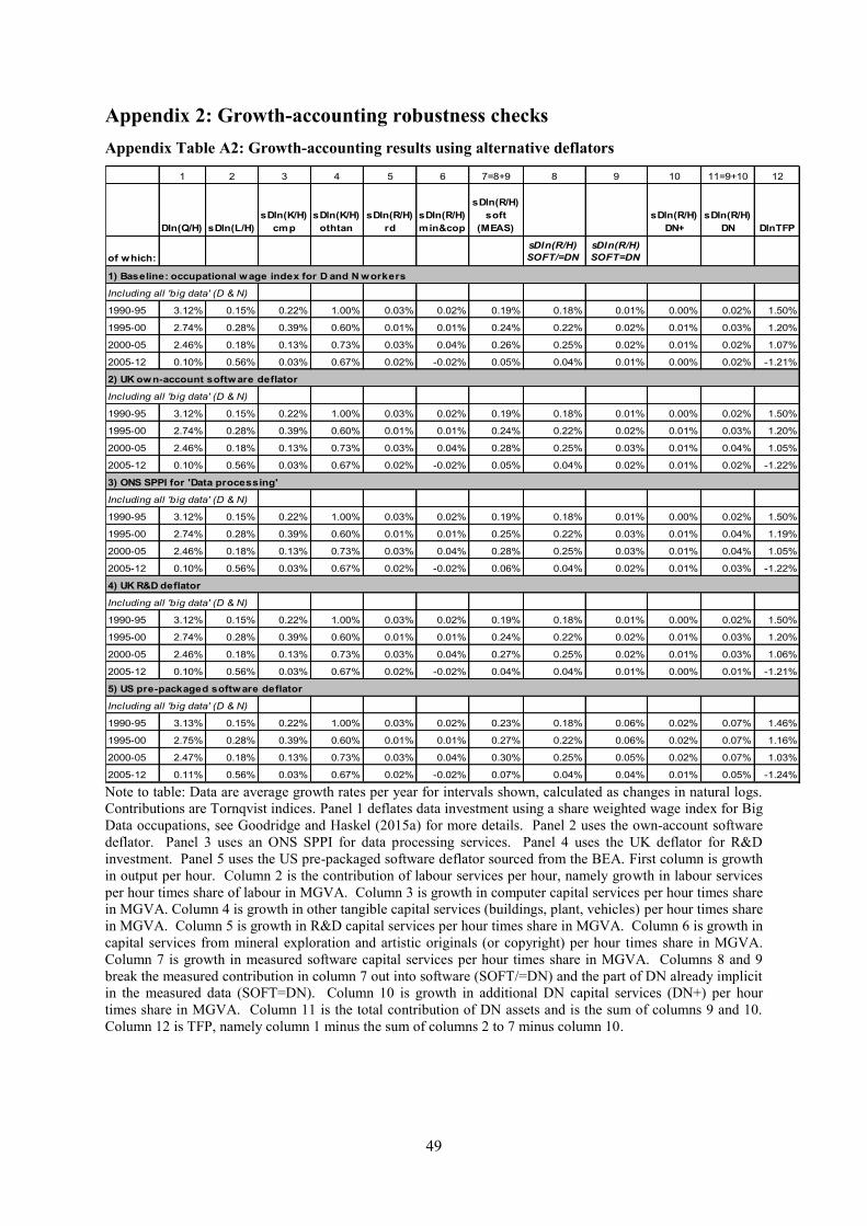
49
Appendix 2: Growth-accounting robustness checks
Appendix Table A2: Growth-accounting results using alternative deflators
1 2 3 4 5 6 7=8+9 8 9 10 11=9+10 12
Dln(Q/H) sDln(L/H)
sDln(K/H)
cmp
sDln(K/H)
othtan
sDln(R/H)
rd
sDln(R/H)
min&cop
sDln(R/H)
soft
(MEAS)
sDln(R/H)
DN+
sDln(R/H)
DN DlnTFP
of which:
sDln(R/H)
SOFT/=DN
sDln(R/H)
SOFT=DN
Including all 'big data' (D & N)
1990-95 3.12% 0.15% 0.22% 1.00% 0.03% 0.02% 0.19% 0.18% 0.01% 0.00% 0.02% 1.50%
1995-00 2.74% 0.28% 0.39% 0.60% 0.01% 0.01% 0.24% 0.22% 0.02% 0.01% 0.03% 1.20%
2000-05 2.46% 0.18% 0.13% 0.73% 0.03% 0.04% 0.26% 0.25% 0.02% 0.01% 0.02% 1.07%
2005-12 0.10% 0.56% 0.03% 0.67% 0.02% -0.02% 0.05% 0.04% 0.01% 0.00% 0.02% -1.21%
Including all 'big data' (D & N)
1990-95 3.12% 0.15% 0.22% 1.00% 0.03% 0.02% 0.19% 0.18% 0.01% 0.00% 0.02% 1.50%
1995-00 2.74% 0.28% 0.39% 0.60% 0.01% 0.01% 0.24% 0.22% 0.02% 0.01% 0.03% 1.20%
2000-05 2.46% 0.18% 0.13% 0.73% 0.03% 0.04% 0.28% 0.25% 0.03% 0.01% 0.04% 1.05%
2005-12 0.10% 0.56% 0.03% 0.67% 0.02% -0.02% 0.05% 0.04% 0.02% 0.01% 0.02% -1.22%
Including all 'big data' (D & N)
1990-95 3.12% 0.15% 0.22% 1.00% 0.03% 0.02% 0.19% 0.18% 0.01% 0.00% 0.02% 1.50%
1995-00 2.74% 0.28% 0.39% 0.60% 0.01% 0.01% 0.25% 0.22% 0.03% 0.01% 0.04% 1.19%
2000-05 2.46% 0.18% 0.13% 0.73% 0.03% 0.04% 0.28% 0.25% 0.03% 0.01% 0.04% 1.05%
2005-12 0.10% 0.56% 0.03% 0.67% 0.02% -0.02% 0.06% 0.04% 0.02% 0.01% 0.03% -1.22%
Including all 'big data' (D & N)
1990-95 3.12% 0.15% 0.22% 1.00% 0.03% 0.02% 0.19% 0.18% 0.01% 0.00% 0.02% 1.50%
1995-00 2.74% 0.28% 0.39% 0.60% 0.01% 0.01% 0.24% 0.22% 0.02% 0.01% 0.03% 1.20%
2000-05 2.46% 0.18% 0.13% 0.73% 0.03% 0.04% 0.27% 0.25% 0.02% 0.01% 0.03% 1.06%
2005-12 0.10% 0.56% 0.03% 0.67% 0.02% -0.02% 0.04% 0.04% 0.01% 0.00% 0.01% -1.21%
Including all 'big data' (D & N)
1990-95 3.13% 0.15% 0.22% 1.00% 0.03% 0.02% 0.23% 0.18% 0.06% 0.02% 0.07% 1.46%
1995-00 2.75% 0.28% 0.39% 0.60% 0.01% 0.01% 0.27% 0.22% 0.06% 0.02% 0.07% 1.16%
2000-05 2.47% 0.18% 0.13% 0.73% 0.03% 0.04% 0.30% 0.25% 0.05% 0.02% 0.07% 1.03%
2005-12 0.11% 0.56% 0.03% 0.67% 0.02% -0.02% 0.07% 0.04% 0.04% 0.01% 0.05% -1.24%
1) Baseline: occupational wage index for D and N workers
2) UK own-account software deflator
5) US pre-packaged software deflator
3) ONS SPPI for 'Data processing'
4) UK R&D deflator
Note to table: Data are average growth rates per year for intervals shown, calculated as changes in natural logs. Contributions are Tornqvist indices. Panel 1 deflates data investment using a share weighted wage index for Big Data occupations, see Goodridge and Haskel (2015a) for more details. Panel 2 uses the own-account software deflator. Panel 3 uses an ONS SPPI for data processing services. Panel 4 uses the UK deflator for R&D investment. Panel 5 uses the US pre-packaged software deflator sourced from the BEA. First column is growth in output per hour. Column 2 is the contribution of labour services per hour, namely growth in labour services per hour times share of labour in MGVA. Column 3 is growth in computer capital services per hour times share in MGVA. Column 4 is growth in other tangible capital services (buildings, plant, vehicles) per hour times share in MGVA. Column 5 is growth in R&D capital services per hour times share in MGVA. Column 6 is growth in capital services from mineral exploration and artistic originals (or copyright) per hour times share in MGVA. Column 7 is growth in measured software capital services per hour times share in MGVA. Columns 8 and 9 break the measured contribution in column 7 out into software (SOFT/=DN) and the part of DN already implicit in the measured data (SOFT=DN). Column 10 is growth in additional DN capital services (DN+) per hour times share in MGVA. Column 11 is the total contribution of DN assets and is the sum of columns 9 and 10. Column 12 is TFP, namely column 1 minus the sum of columns 2 to 7 minus column 10.
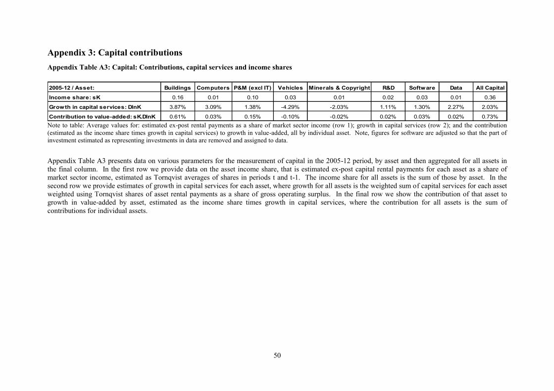
50
Appendix 3: Capital contributions
Appendix Table A3: Capital: Contributions, capital services and income shares
2005-12 / Asset: Buildings Computers P&M (excl IT) Vehicles Minerals & Copyright R&D Software Data All Capital
Income share: sK 0.16 0.01 0.10 0.03 0.01 0.02 0.03 0.01 0.36
Growth in capital services: DlnK 3.87% 3.09% 1.38% -4.29% -2.03% 1.11% 1.30% 2.27% 2.03%
Contribution to value-added: sK.DlnK 0.61% 0.03% 0.15% -0.10% -0.02% 0.02% 0.03% 0.02% 0.73%
Note to table: Average values for: estimated ex-post rental payments as a share of market sector income (row 1); growth in capital services (row 2); and the contribution (estimated as the income share times growth in capital services) to growth in value-added, all by individual asset. Note, figures for software are adjusted so that the part of investment estimated as representing investments in data are removed and assigned to data.
Appendix Table A3 presents data on various parameters for the measurement of capital in the 2005-12 period, by asset and then aggregated for all assets in the final column. In the first row we provide data on the asset income share, that is estimated ex-post capital rental payments for each asset as a share of market sector income, estimated as Tornqvist averages of shares in periods t and t-1. The income share for all assets is the sum of those by asset. In the second row we provide estimates of growth in capital services for each asset, where growth for all assets is the weighted sum of capital services for each asset weighted using Tornqvist shares of asset rental payments as a share of gross operating surplus. In the final row we show the contribution of that asset to growth in value-added by asset, estimated as the income share times growth in capital services, where the contribution for all assets is the sum of contributions for individual assets.

This paper has been produced by the Department of Management at Imperial College Business School
Copyright © the authors 2014 All rights reserved
ISSN: 1744-6783
Imperial College Business School
Tanaka Building South Kensington Campus London SW7 2AZ United Kingdom
T: +44 (0)20 7589 5111 F: +44 (0)20 7594 9184
www.imperial.ac.uk/business-school
This work is licensed under a Creative Commons Attribution 4.0 International License.