Coordination, Moderation, and Institutional Balancing in American

Presidential and House Elections

by

Walter R. Mebane, Jr.

Cornell University

forthcoming, American Political Science Review

Abstract

Voters have been coordinating their choices for President and House of Representatives in recent

presidential election years, with each voter using a strategy that features policy moderation.

Coordination is de�ned as a noncooperative rational expectations equilibrium among voters, in

which each voter has both common knowledge and private information about the election

outcome. Stochastic choice models estimated using individual-level NES data from 1976{96

support coordination versus a model in which voters act nonstrategically to moderate policy. The

empirical coordinating model satis�es the �xed-point condition that de�nes the common

knowledge expectation voters have about the outcome in the theoretical equilibrium. The

proportion of voters who split their tickets in order to balance the House with the President has

been small but large enough to a�ect election outcomes. Moderation has usually been based on

voters' expectations that the President will be at least an equal of the House in determining

postelection policy.

Do Americans coordinate their votes for President and for Congress? Suppose a voter knows

that policy outcomes are compromises between the positions taken by the President and Congress

and believes the two political parties push for distinct policy alternatives. Then the voter believes

that di�erent combinations of party control of the presidency and Congress will produce di�erent

policy outcomes. If the voter cares about the policy outcomes, then the voter's choices among

candidates should depend on the combination of party control the choices will help bring about.

Some voters would do best to vote a party-line, straight ticket, while others would do best to split

their tickets to try to bring about a \moderate" policy outcome, that is, an outcome in some sense

between the parties' positions (Alesina and Rosenthal 1989, 1995, 1996; Fiorina 1988, 1992, 73{81;

Ingberman and Villani 1993). To cast the most e�ective vote, each voter should consider how likely

it is that the election will produce each possible combination of party control. Coordination occurs

when each voter makes the best possible assessment of what the election outcome will be and then

uses that assessment to choose candidates in the way most likely to produce the best possible result

for the voter.

Moderation does not necessarily imply coordination. Moderation refers to the relationship

between the policy outcome intended by the voter and the parties' policy positions. There is

moderation if the intended policy outcome is an intermediate combination of the parties' positions.

Coordination refers to a relationship among di�erent voters' choices among candidates.1 There is

coordination if each voter's choice is in a strategic sense in equilibrium with every other voter's

choice. I interpret this to mean three things: Each voter's strategy for choosing among candidates is

in equilibrium with every other voter's strategy for choosing among candidates; each voter's beliefs

about every other voter's preferences and strategy are compatible with the voter's own strategy;

and each voter's beliefs are compatible with every other voter's beliefs.

Coordination among voters is not the same as cooperation among them. In a �nancial market,

1

economic agents who possess private information and act strategically may coordinate their deci-

sions to buy or sell based on the system of prices that all agents know, without the need for sets of

agents to reach binding prior agreements about how to act. The information that the agents have in

common may be enough to let the market operate in a state of strategic equilibrium among agents

(e.g., Grossman 1989). In the theoretical model I develop in this article, voters do not cooperate;

each voter is able to make an equilibrium strategic choice among candidates, in accurate antici-

pation of the aggregate result of the choices all other voters intend to make, by using information

that all voters know. Alesina and Rosenthal's (1989, 1995, 1996) theory of moderation features

coordination|each voter's choice depends on an expected election result that everyone knows and

that is an equilibrium|but Fiorina's (1988, 1992, 73{81) theory does not (Alesina and Rosenthal

1995, 66{71). In Fiorina's theory, voters do not act strategically at all. Voters act strategically

in Alesina and Rosenthal's treatment, but no one has any private information about the election

outcome. In the model developed here, di�erent voters have beliefs about the upcoming election

results that are very similar but not exactly the same in equilibrium. The similarity is a result of

the common knowledge they have, while the di�erences that remain are due to private information

each voter has about concerns that a�ect the voter's preferences among candidates.

I use National Election Study (NES) data from presidential election years 1976 through 1996

to estimate a stochastic choice model that closely matches the theoretical model. Based on the

empirical results, I argue that in recent years American voters' choices for President and the House

of Representatives have been coordinated, with each voter using a strategy that features policy

moderation. In both the theoretical model and the empirical model, each voter forms preferences

about the candidates based on a personally distinct idea about what the parties' policy positions

are. The coordination takes the form of a rational expectations equilibrium among voters. The

notion of voter equilibrium here is similar to the concept of a \ful�lled expectations" equilibrium

2

(Kreps 1977) developed for elections by McKelvey and Ordeshook (1984, 1985a, 1985b).2

The models of moderation-with-coordination developed by Alesina and Rosenthal (1989, 1995,

1996) have implications for the midterm loss phenomenon and for election-related uctuations in

economic phenomena such as growth. The latter have been tested using aggregate time-series data,

with mostly positive results (Alesina, Londregan, and Rosenthal 1993; Alesina and Rosenthal 1995;

Alesina, Roubini, and Cohen 1997).

Evidence that individuals coordinate has been lacking. Several authors report individual-level

(Alvarez and Schousen 1993; Born 1994a) or aggregate-level (Burden and Kimbal 1998; Frymer

1994) tests aimed at Fiorina's (1988; 1992, 73{81) theory of moderation, with controversially (Born

1994b; Fiorina 1994) negative results. As previously noted, Fiorina's theory does not posit coor-

dination among voters. The tests of his theory have not examined whether voters' expectations

about the election outcomes a�ect their choices. I use the NES data to estimate a stochastic choice

model that implements Fiorina's theory and test it against the coordinating model.

The heart of the formal model of coordination that I develop and test empirically is a �xed-

point theorem that de�nes the common knowledge belief that all voters have about the upcoming

election results. The election results are summarized in the values of two aggregate statistics: (i)

the proportion of the two-party vote to be cast nationally for Republican candidates for the House

and (ii) the probability that the Republican presidential candidate will defeat the Democrat. Each

voter cares about those values because they a�ect the loss each voter expects to experience from

policies the government will adopt after the election. Each voter chooses among candidates so as

to minimize that loss. Therefore, each voter's belief about the aggregate values a�ects the voter's

choices. In general, if there is a single pair of values that every voter believes the aggregate statistics

to have and every voter chooses based on that belief, then the aggregate result of all their choices

may be expected to di�er from the values they all believed. In that case, beliefs and expected actions

3

are inconsistent with one another. The �xed-point result demonstrates that a pair of aggregate

values exists for which there is no such inconsistency: When every voter chooses based on belief in

the �xed-point aggregate values, the aggregate result to be expected from all their choices is the very

same pair of aggregate values. In that case, beliefs match expected actions. Common knowledge

of the �xed-point values is not quite enough to establish an equilibrium, because the common

knowledge does not include private information each voter has about the voter's actual choice. If

each voter's belief equals the common knowledge values adjusted by amounts that correspond to

the voter's choices, then the belief each voter has about the aggregate result is consistent with

the choices the voter knows it will make. Despite knowing that every other voter is also acting

on the basis of beliefs that di�er slightly from the common knowledge values, no voter knows any

other voter's private information, and so no voter can do any better than to use the common

knowledge values as its aggregate expectation for what everyone else is going to do. Because all

voters are situated similarly, it is common knowledge that every voter is forming beliefs in that way.

Thus there is an equilibrium in which every voter has a slightly di�erent expectation regarding the

upcoming election results.

The �xed-point result that determines what voters' beliefs are in equilibrium in the theoretical

model imposes a constraint on the statistical model to be used to estimate the parameters of the

model with survey data. The empirical model is de�ned to correspond as closely as possible to

the theoretical model. Both models use the same functional forms for each voter's loss function

as well as the same speci�cations for the statistical distribution of the random disturbances that

a�ect the candidate choices each voter makes. Hence, both models specify the same stochastic

choice model for each voter. The special constraint is that the estimates of the parameters of the

empirical model must be such that the aggregate election summary statistics estimated from the

survey data satisfy the �xed-point condition. Stochastic choice models of electoral behavior have

4

not previously imposed such a constraint, and its introduction here is an important innovation in

the empirical model speci�cation. The empirically determined �xed-point values are the estimates

for the aggregate values that are common knowledge in equilibrium in the theoretical model. A

distinction between the empirical and theoretical models is that, because of limitations on what we

can observe with survey data, the empirical model treats the �xed-point values as the belief that

every voter has regarding the upcoming election outcome. The empirical model does not re�ne

each voter's belief to take the voter's private information into account.

The theoretical and empirical models use assumptions about what individual voters know that

are unquestionably unrealistic and unbelievable. It may help to put both the theory and the

empirical �ndings in what I think is the most productive perspective if I say something about this

at the outset. In the Conclusion, I brie y outline how in reality a coordinating voting equilibrium

must depend on a collection of institutions to aggregate and broadcast information that the current

model treats as common knowledge among voters. My analysis is therefore implicitly conditional

on the existence of an appropriate institutional context. In a way that I touch on brie y in the

Conclusion,3 I think voters possess a variety of beliefs about things the current model treats as

common knowledge; the values that are common knowledge in the current model are more like the

mean of the distribution of individuals' beliefs than they are values that every individual actually

possesses. Even if the current model correctly characterizes the mean, it understates the variability

across individuals.

A Model of Coordinating Voting with Moderation

The model treats the election as a game among all voters, assumed to be a large number. Voters

act noncooperatively. The model focuses on the choices each voter makes between two candidates

for President and two candidates for a House seat. The votes for President occur in the context of

5

the Electoral College. There are many House districts, but each voter votes in only one of them.

There are two parties, Democratic and Republican, and each race has one candidate running for

each party. Both whether an incumbent is running and the incumbent's party vary over districts.

Each voter's preferences regarding pairs of candidates depend on the expected election outcome

and, therefore, on the choice strategy every other voter is using. Equilibrium occurs when, given

everything each voter knows|including the voter's own intended choice and accurate expectations

regarding other voters' strategies|no voter expects to gain by using a di�erent strategy.

The preferences each voter has regarding the candidates are based in part on spatial comparisons

between the voter's ideal point and the policies the voter believes will result from various election

outcomes. Those policies are functions of the policy position the voter expects each party will act

on after the election. The expected post-election policy position for each party is a combination

of two positions that may di�er: the position the voter associates with the party on the basis

of previous turns in o�ce and previous campaigns, and the position the voter thinks the party's

current presidential candidate has adopted. All presidential candidates do not have the same ability

to move their parties to the position the candidate supports. For each election, the expected party

position is a weighted average of the candidate's position and the prior party position. The more

in uential the candidate, the greater is the weight of the candidate's position.

I use #Di, #Ri, #PDi, and #PRi to denote values in the interval [0; 1] that voter i, i = 1; : : : ; N ,

has in mind at election time for the prior position of the Democratic party (#Di) and Republican

party (#Ri) and for the position of the Democratic presidential candidate (#PDi) and Republican

presidential candidate (#PRi). The Democratic positions need not be to the \left" of (i.e., numer-

ically less than) the Republican positions. The policy positions voter i expects the Democratic

6

party and the Republican party to act on after the election are, respectively,

�Di = �D#PDi + (1� �D)#Di ; 0 � �D � 1 ; (1a)

�Ri = �R#PRi + (1� �R)#Ri ; 0 � �R � 1 : (1b)

If the Democratic party's position is expected to be very close to that of its presidential candidate,

then the weight �D is near one. If the Democratic party's position is expected to remain close to

its previous value, then �D is near zero. The parameter �R has an analogous relationship to the

position voter i expects the Republican party to act on after the election.

The policy expected to result from each possible election outcome depends on four factors:

the parties' expected policy positions (just de�ned); the position expected to be supported in

Congress; the President's strength in comparison to the House; and which party's candidate is

elected President. To represent the expected position of Congress, I simplify by ignoring both

the Senate and all internal structure in the House, such as seats, committees, bills, and rules;

the expected position of the House is simply a weighted average of the expected positions of the

two parties. Each party's weight is equal to the proportion of the vote that i expects to be

cast nationally for the party's House candidates. Using �Hi to denote the expected Republican

proportion, the expected position of the House is �Hi�Ri + (1� �Hi)�Di.

The postelection policy expected given any particular value of �Hi is then a weighted average of

the expected position of the House and the expected position of the President's party. The weight

of the President represents the President's strength in comparison to the House. For each value of

�Hi there are two expectations for postelection policy, depending on the President's party:

~�Di = �D�Di + (1� �D)[ �Hi�Ri + (1� �Hi)�Di] ; 0 � �D � 1 ; (2a)

~�Ri = �R�Ri + (1� �R)[ �Hi�Ri + (1� �Hi)�Di] ; 0 � �R � 1 : (2b)

Policy ~�Di is expected to occur if a Democrat is President, and policy ~�Ri is expected to occur if

7

a Republican is President. The weights, �D and �R, represent the strength a President from each

party is expected to have. The value �D = 1 means that a Democratic President is expected to

dictate policy, so that the legislature would play no role, while �D = 0 means that the legislature

is expected to determine policy, with the President being irrelevant. The interpretation of �R is

analogous for a Republican President. The functional forms of ~�Di and ~�Ri are essentially the same

as the simplest policymaking formalism considered by Alesina and Rosenthal (1995, 47{8).

The preference each voter has for each possible election outcome is measured by the loss the

voter expects given that outcome. The loss depends on the absolute discrepancy between the voter's

ideal point, denoted �i 2 [0; 1], and the policy expected given the election outcome. The absolute

discrepancy is j�i� ~�Dij with a Democratic President and j�i� ~�Rij with a Republican President. A

voter's expected loss always increases as the absolute discrepancy between the voter's ideal point

and the expected policy gets larger.

I use a functional form for the loss that is exible in two ways. First, an exponent q > 0 allows

the loss to be a concave (0 < q < 1), linear (q = 1), or convex (q > 1) function of the absolute

discrepancy between �i and each expected policy. Second, a variable �i, 0 < �i < 1, represents the

possibility that voters do not treat the two discrepancies equally. If �i <12 (�i =

12 , �i >

12), voter i

weights a discrepancy associated with a Republican President more than (the same as, less than) a

discrepancy of the same magnitude associated with a Democratic President. The voter's expected

losses with, respectively, a Democratic and a Republican President are

�Di = �ij�i � ~�Dijq + �Di ;

�Ri = (1� �i)j�i � ~�Rijq + �Ri ;

where the continuous random variables �Di and �Ri represent other things besides the policy-related

discrepancies that a�ect the voter's expected loss.

At the time of the election, the voter does not know for sure which candidate will be elected

8

President. I assume that the voter computes an expectation for the expected loss, by using the

probability that each candidate will win in a standard expected-value formula. �Pi denotes voter i's

expectation for the probability that the Republican wins. The voter's expected loss is

�i = (1� �Pi)�ij�i � ~�Dijq + �Pi(1� �i)j�i � ~�Rij

q + �i ; (3)

where �i = (1� �Pi)�Di + �Pi�Ri.

The speci�cations of equations 2a, 2b and 3 have functional forms that are quite similar to those

used by Alesina and Rosenthal (1995), but there is an important di�erence in what the current

model says about the information that voters have. The speci�cations of equations 2a, 2b and 3

di�er from Alesina and Rosenthal's (1995) theory in allowing the expected policies ~�Di and ~�Ri

and the expected election outcomes �Hi and �Pi to vary over voters. In the theory of Alesina and

Rosenthal (1995, 1996), the expected policies and expected election outcomes have values that all

voters have identically in common. The variations in the values over voters in the current model

mean that the current model endows voters with private information in a way that the theory of

Alesina and Rosenthal (1995, 1996) essentially does not do. The current model therefore in an

important way generalizes the approach taken by Alesina and Rosenthal (1995, 1996).

A voter chooses the pair of candidates|one candidate for President and one for the House|

that minimizes the voter's expected loss, �i. I measure the e�ect on �i of choosing any one pair,

as follows. Let �Pi;R denote the expected probability that the Republican presidential candidate

wins if the voter chooses the Republican, and let �Pi;D denote the probability that the Republican

wins if the voter chooses the Democrat. Because the e�ect of a single voter's choice on �Pi is very

small, the e�ect on �i of the voter's choosing the Republican presidential candidate rather than

the Democrat is well approximated by ( �Pi;R � �Pi;D)d�i=d �Pi.4 If ( �Pi;R � �Pi;D)d�i=d �Pi is positive,

then voting for the Republican increases the voter's expected loss. Likewise, let �Hi;R ( �Hi;D) be

the proportion of the national two-party vote received by Republican House candidates if the voter

9

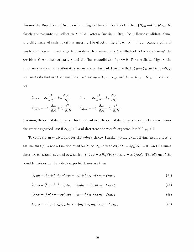
chooses the Republican (Democrat) running in the voter's district. Then ( �Hi;R � �Hi;D)d�i=d �Hi

closely approximates the e�ect on �i of the voter's choosing a Republican House candidate. Sums

and di�erences of such quantities measure the e�ect on �i of each of the four possible pairs of

candidate choices. I use �i;ph to denote such a measure of the e�ect of voter i's choosing the

presidential candidate of party p and the House candidate of party h. For simplicity, I ignore the

di�erences in voter population sizes across States. Instead, I assume that �Pi;R� �Pi;D and �Hi;R� �Hi;D

are constants that are the same for all voters: bP = �Pi;R � �Pi;D and bH = �Hi;R� �Hi;D. The e�ects

are

�i;RR = bPd�id �Pi

+ bHd�id �Hi

; �i;RD = bPd�id �Pi

� bHd�id �Hi

;

�i;DR = �bPd�id �Pi

+ bHd�id �Hi

; �i;DD = �bPd�id �Pi

� bHd�id �Hi

:

Choosing the candidate of party p for President and the candidate of party h for the House increases

the voter's expected loss if �i;ph > 0 and decreases the voter's expected loss if �i;ph < 0.

To compute an explicit rule for the voter's choice, I make two more simplifying assumptions. I

assume that �i is not a function of either �Pi or �Hi, so that d�i=d �Pi = d�i=d �Hi = 0. And I assume

there are constants bHP and bPH such that bHP = d �Hi=d �Pi and bPH = d �Pi=d �Hi. The e�ects of the

possible choices on the voter's expected losses are then

�i;RR = (bP + bHbPH)wPi + (bH + bPbHP )wHi + �RRi ; (4a)

�i;RD = (bP � bHbPH)wPi + (bP bHP � bH)wHi + �RDi ; (4b)

�i;DR = (bHbPH � bP )wPi + (bH � bPbHP )wHi + �DRi ; (4c)

�i;DD = �(bP + bHbPH)wPi � (bH + bP bHP )wHi + �DDi ; (4d)

10

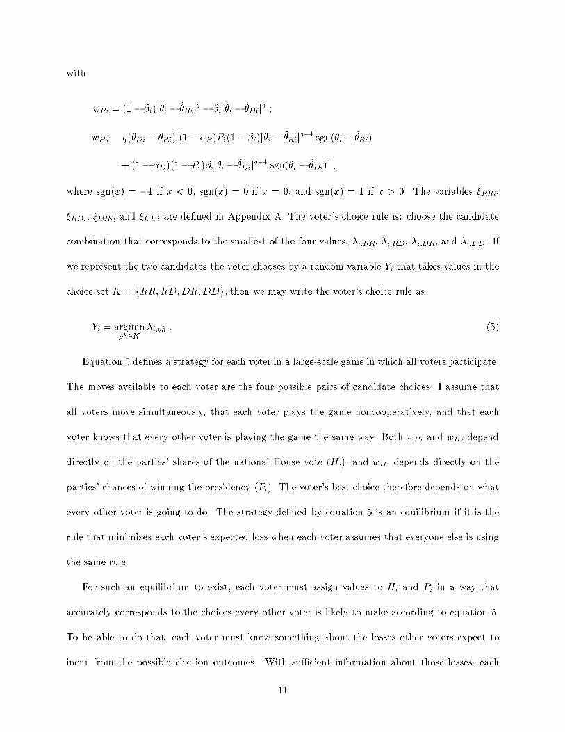
with

wPi = (1� �i)j�i � ~�Rijq � �ij�i � ~�Dij

q ;

wHi = q(�Di � �Ri)[(1� �R) �Pi(1� �i)j�i � ~�Rijq�1 sgn(�i � ~�Ri)

+ (1� �D)(1� �Pi)�ij�i � ~�Dijq�1 sgn(�i � ~�Di)] ;

where sgn(x) = �1 if x < 0, sgn(x) = 0 if x = 0, and sgn(x) = 1 if x > 0. The variables �RRi,

�RDi, �DRi, and �DDi are de�ned in Appendix A. The voter's choice rule is: choose the candidate

combination that corresponds to the smallest of the four values, �i;RR, �i;RD, �i;DR, and �i;DD. If

we represent the two candidates the voter chooses by a random variable Yi that takes values in the

choice set K = fRR;RD;DR;DDg, then we may write the voter's choice rule as

Yi = argminph2K

�i;ph : (5)

Equation 5 de�nes a strategy for each voter in a large-scale game in which all voters participate.

The moves available to each voter are the four possible pairs of candidate choices. I assume that

all voters move simultaneously, that each voter plays the game noncooperatively, and that each

voter knows that every other voter is playing the game the same way. Both wPi and wHi depend

directly on the parties' shares of the national House vote ( �Hi), and wHi depends directly on the

parties' chances of winning the presidency ( �Pi). The voter's best choice therefore depends on what

every other voter is going to do. The strategy de�ned by equation 5 is an equilibrium if it is the

rule that minimizes each voter's expected loss when each voter assumes that everyone else is using

the same rule.

For such an equilibrium to exist, each voter must assign values to �Hi and �Pi in a way that

accurately corresponds to the choices every other voter is likely to make according to equation 5.

To be able to do that, each voter must know something about the losses other voters expect to

incur from the possible election outcomes. With su�cient information about those losses, each

11

voter can anticipate what other voters will do in response to each electoral circumstance that may

arise. Knowledge of that response pattern allows each i to determine the mutually consistent values

of �Hi and �Pi. The pair ( �Hi; �Pi) is mutually consistent if, given everything i knows, i chooses in such

a way that|taking i's own choice into account|the proportion Republican that i expects among

votes for the House is �Hi and the probability with which i expects the Republican presidential

candidate to win is �Pi. In equilibrium, all pairs ( �Hi; �Pi), i = 1; : : : ; N , are mutually consistent.

I assume it is common knowledge (Fudenberg and Tirole 1991, 541{6) that every voter i has an

expected loss �i as de�ned by equation 3, and that every i is choosing candidates so as to minimize

�i. I assume that the common knowledge includes the values of all parameters, including �D, �R,

�D, �R, q, bP , bH , bPH , bHP , and any parameters in �i, �RRi, �RDi, �DRi, or �DDi. It is then

common knowledge that, for some values of the policy position and other variables, equation 5 is

every voter's choice rule.

No voter knows the values of the ideal point, the party or presidential candidate policy positions,

or the other variables on the basis of which any other voter is choosing via equation 5. Each voter

does know the probability distribution of those values. Let Zi be an ordered set that includes

all the observable variables in �i;RR, �i;RD, �i;DR, and �i;DD. That includes �i, #Di, #Ri, #PDi,

and #PRi; any variables that make up �i; and the component zphi of each �phi, ph 2 K, that

may be observed using some generally known technology (e.g., an opinion survey). There are

M � N mutually exclusive and exhaustive groups of voters, denoted Vk, k = 1; : : : ;M . For every

voter i 2 Vk, the election-time value of Zi is generated, independently across individuals, by a

process that takes values in a set ~Z and has unimodal probability measure fk,R~Z dfk(Zi) = 1. Let

�phi denote the component of �phi not covered by Zi, ph 2 K. These variables|collectively, the

disturbance �i = (�RRi; �RDi; �DRi; �DDi)|have a joint probability distribution that is the same for

12

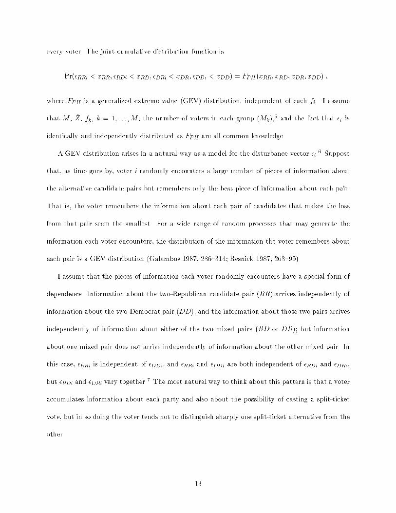
every voter. The joint cumulative distribution function is

Pr(�RRi < xRR; �RDi < xRD; �DRi < xDR; �DDi < xDD) = FPH (xRR; xRD; xDR; xDD) ;

where FPH is a generalized extreme value (GEV) distribution, independent of each fk . I assume

that M , ~Z , fk, k = 1; : : : ;M , the number of voters in each group (Mk),5 and the fact that �i is

identically and independently distributed as FPH are all common knowledge.

A GEV distribution arises in a natural way as a model for the disturbance vector �i.6 Suppose

that, as time goes by, voter i randomly encounters a large number of pieces of information about

the alternative candidate pairs but remembers only the best piece of information about each pair.

That is, the voter remembers the information about each pair of candidates that makes the loss

from that pair seem the smallest. For a wide range of random processes that may generate the

information each voter encounters, the distribution of the information the voter remembers about

each pair is a GEV distribution (Galambos 1987, 286{314; Resnick 1987, 263{90).

I assume that the pieces of information each voter randomly encounters have a special form of

dependence. Information about the two-Republican candidate pair (RR) arrives independently of

information about the two-Democrat pair (DD), and the information about those two pairs arrives

independently of information about either of the two mixed pairs (RD or DR); but information

about one mixed pair does not arrive independently of information about the other mixed pair. In

this case, �RRi is independent of �DDi, and �RRi and �DDi are both independent of �RDi and �DRi,

but �RDi and �DRi vary together.7 The most natural way to think about this pattern is that a voter

accumulates information about each party and also about the possibility of casting a split-ticket

vote, but in so doing the voter tends not to distinguish sharply one split-ticket alternative from the

other.

13

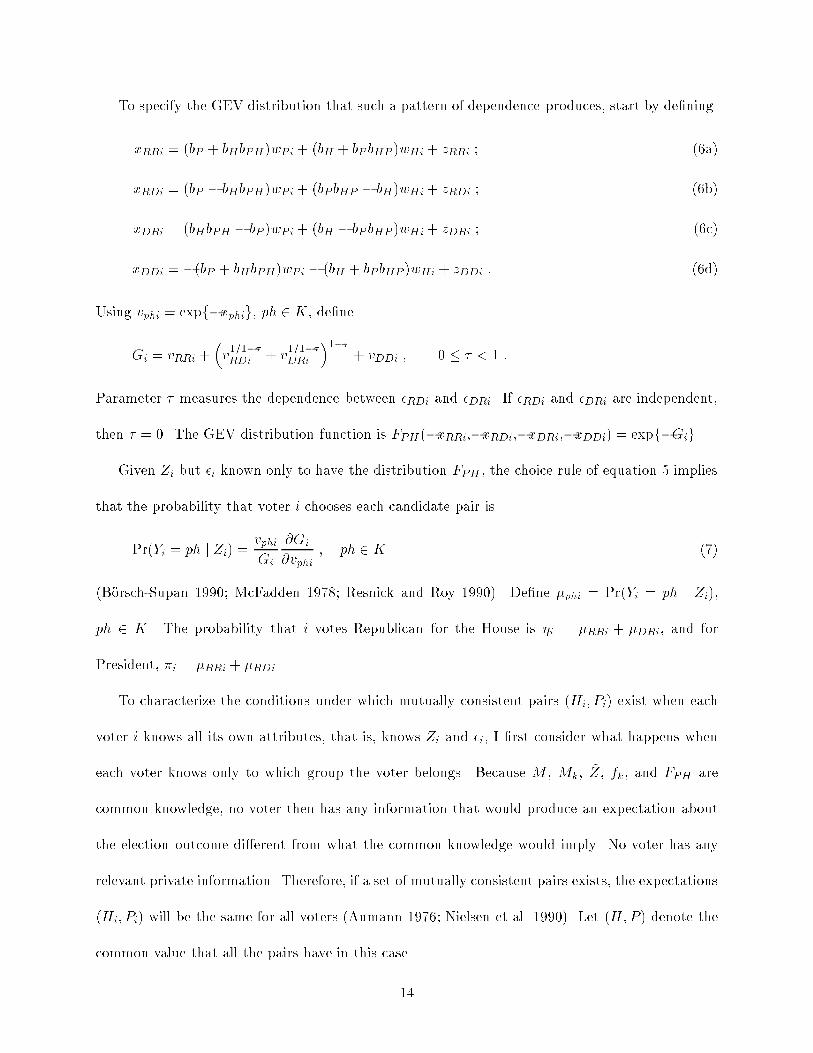
To specify the GEV distribution that such a pattern of dependence produces, start by de�ning

xRRi = (bP + bHbPH)wPi + (bH + bP bHP )wHi+ zRRi ; (6a)

xRDi = (bP � bHbPH)wPi + (bPbHP � bH)wHi+ zRDi ; (6b)

xDRi = (bHbPH � bP )wPi + (bH � bP bHP )wHi+ zDRi ; (6c)

xDDi = �(bP + bHbPH)wPi � (bH + bPbHP )wHi + zDDi : (6d)

Using vphi = expf�xphig, ph 2 K, de�ne

Gi = vRRi +�v1=1��RDi + v

1=1��DRi

�1��+ vDDi ; 0 � � < 1 :

Parameter � measures the dependence between �RDi and �DRi. If �RDi and �DRi are independent,

then � = 0. The GEV distribution function is FPH(�xRRi,�xRDi,�xDRi,�xDDi) = expf�Gig.

Given Zi but �i known only to have the distribution FPH , the choice rule of equation 5 implies

that the probability that voter i chooses each candidate pair is

Pr(Yi = ph j Zi) =vphiGi

@Gi

@vphi; ph 2 K (7)

(B�orsch-Supan 1990; McFadden 1978; Resnick and Roy 1990). De�ne �phi = Pr(Yi = ph j Zi),

ph 2 K. The probability that i votes Republican for the House is �i = �RRi + �DRi, and for

President, �i = �RRi + �RDi.

To characterize the conditions under which mutually consistent pairs ( �Hi; �Pi) exist when each

voter i knows all its own attributes, that is, knows Zi and �i, I �rst consider what happens when

each voter knows only to which group the voter belongs. Because M , Mk, ~Z, fk , and FPH are

common knowledge, no voter then has any information that would produce an expectation about

the election outcome di�erent from what the common knowledge would imply. No voter has any

relevant private information. Therefore, if a set of mutually consistent pairs exists, the expectations

( �Hi; �Pi) will be the same for all voters (Aumann 1976; Nielsen et al. 1990). Let ( �H; �P) denote the

common value that all the pairs have in this case.

14

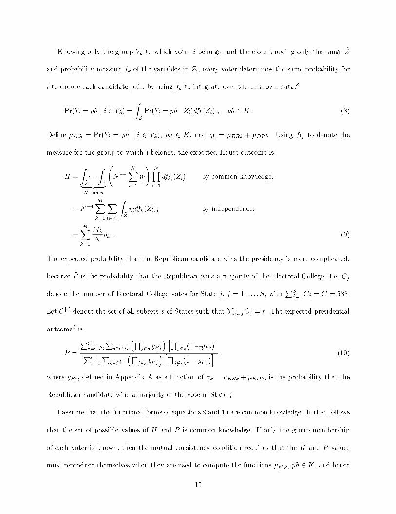
Knowing only the group Vk to which voter i belongs, and therefore knowing only the range ~Z

and probability measure fk of the variables in Zi, every voter determines the same probability for

i to choose each candidate pair, by using fk to integrate over the unknown data:8

Pr(Yi = ph j i 2 Vk) =

Z~ZPr(Yi = ph j Zi)dfk(Zi) ; ph 2 K : (8)

De�ne ��phk = Pr(Yi = ph j i 2 Vk), ph 2 K, and ��k = ��RRk + ��DRk . Using fki to denote the

measure for the group to which i belongs, the expected House outcome is

�H =

Z~Z� � �

Z~Z| {z }

N times

N�1

NXi=1

�i

!NYi=1

dfki(Zi); by common knowledge,

= N�1MXk=1

Xi2Vk

Z~Z�idfk(Zi); by independence,

=MXk=1

Mk

N��k : (9)

The expected probability that the Republican candidate wins the presidency is more complicated,

because �P is the probability that the Republican wins a majority of the Electoral College. Let Cj

denote the number of Electoral College votes for State j, j = 1; : : : ; S, withPS

j=1 Cj = C = 538.

Let C[r] denote the set of all subsets s of States such thatP

j2sCj = r. The expected presidential

outcome9 is

�P =

PCr=C=2

Ps2C[r]

�Qj2s �yPj

� hQj 62s(1� �yPj)

iPC

r=0

Ps2C[r]

�Qj2s �yPj

� hQj 62s(1� �yPj)

i ; (10)

where �yPj , de�ned in Appendix A as a function of ��k = ��RRk + ��RDk, is the probability that the

Republican candidate wins a majority of the vote in State j.

I assume that the functional forms of equations 9 and 10 are common knowledge. It then follows

that the set of possible values of �H and �P is common knowledge. If only the group membership

of each voter is known, then the mutual consistency condition requires that the �H and �P values

must reproduce themselves when they are used to compute the functions ��phk, ph 2 K, and hence

15

equations 9 and 10. In technical terms, the pair of computed values must be a �xed point of the

mapping [0; 1]� [0; 1] ! [0; 1]� [0; 1] that equations 9 and 10 specify. In Appendix A (Theorem

2) I show that such a pair ( �H; �P ) always exists (except on a set of measure zero). Necessary or

su�cient conditions for �H and �P to be uniquely determined by the parameters of the model and

the measures fk are not clear.

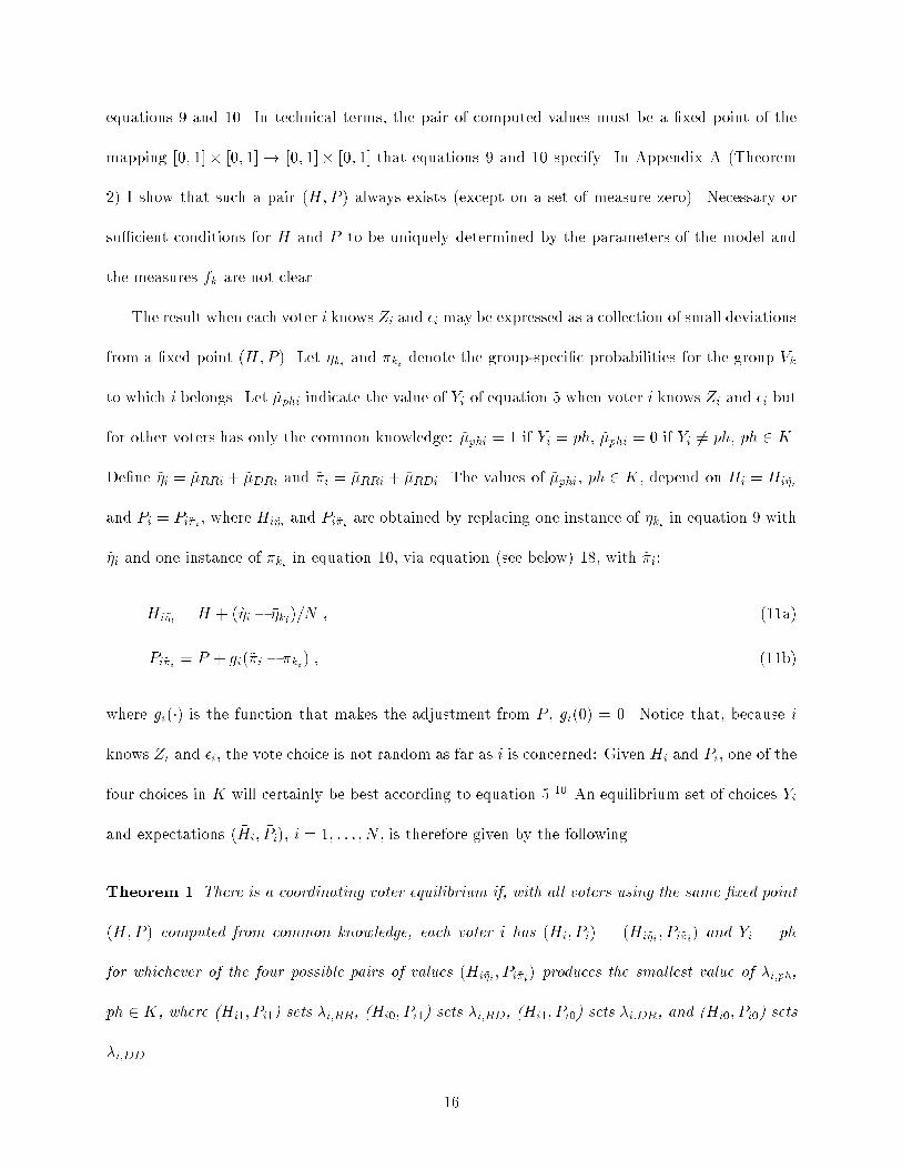
The result when each voter i knows Zi and �i may be expressed as a collection of small deviations

from a �xed point ( �H; �P). Let ��ki and ��ki denote the group-speci�c probabilities for the group Vk

to which i belongs. Let ~�phi indicate the value of Yi of equation 5 when voter i knows Zi and �i but

for other voters has only the common knowledge: ~�phi = 1 if Yi = ph, ~�phi = 0 if Yi 6= ph, ph 2 K.

De�ne ~�i = ~�RRi + ~�DRi and ~�i = ~�RRi + ~�RDi. The values of ~�phi, ph 2 K, depend on �Hi = �Hi~�i

and �Pi = �Pi~�i , where�Hi~�i and

�Pi~�i are obtained by replacing one instance of ��ki in equation 9 with

~�i and one instance of ��ki in equation 10, via equation (see below) 18, with ~�i:

�Hi~�i =�H + (~�i � ��ki)=N ; (11a)

�Pi~�i =�P + gi(~�i � ��ki) ; (11b)

where gi(�) is the function that makes the adjustment from �P , gi(0) = 0. Notice that, because i

knows Zi and �i, the vote choice is not random as far as i is concerned: Given �Hi and �Pi, one of the

four choices in K will certainly be best according to equation 5.10 An equilibrium set of choices Yi

and expectations ( �Hi; �Pi), i = 1; : : : ; N , is therefore given by the following.

Theorem 1 There is a coordinating voter equilibrium if, with all voters using the same �xed point

( �H; �P ) computed from common knowledge, each voter i has ( �Hi; �Pi) = ( �Hi~�i ;�Pi~�i) and Yi = ph

for whichever of the four possible pairs of values ( �Hi~�i;�Pi~�i) produces the smallest value of �i;ph,

ph 2 K, where ( �Hi1; �Pi1) sets �i;RR, ( �Hi0; �Pi1) sets �i;RD, ( �Hi1; �Pi0) sets �i;DR, and ( �Hi0; �Pi0) sets

�i;DD.

16

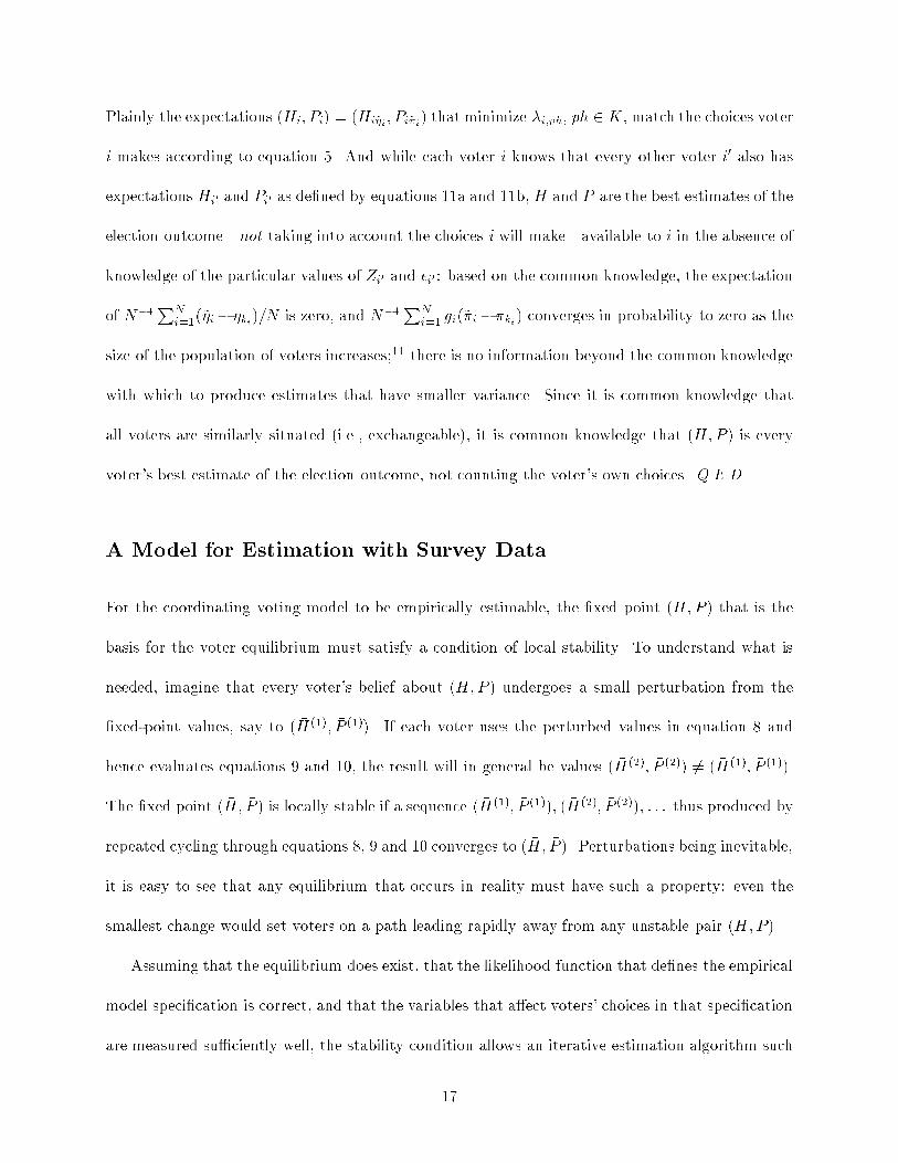
Plainly the expectations ( �Hi; �Pi) = ( �Hi~�i ;�Pi~�i) that minimize �i;ph, ph 2 K, match the choices voter

i makes according to equation 5. And while each voter i knows that every other voter i0 also has

expectations �Hi0 and �Pi0 as de�ned by equations 11a and 11b, �H and �P are the best estimates of the

election outcome|not taking into account the choices i will make|available to i in the absence of

knowledge of the particular values of Zi0 and �i0 : based on the common knowledge, the expectation

of N�1PN

i=1(~�i� ��ki)=N is zero, and N�1PN

i=1 gi(~�i� ��ki) converges in probability to zero as the

size of the population of voters increases;11 there is no information beyond the common knowledge

with which to produce estimates that have smaller variance. Since it is common knowledge that

all voters are similarly situated (i.e., exchangeable), it is common knowledge that ( �H; �P ) is every

voter's best estimate of the election outcome, not counting the voter's own choices. Q.E.D.

A Model for Estimation with Survey Data

For the coordinating voting model to be empirically estimable, the �xed point ( �H; �P ) that is the

basis for the voter equilibrium must satisfy a condition of local stability. To understand what is

needed, imagine that every voter's belief about ( �H; �P ) undergoes a small perturbation from the

�xed-point values, say to ( �H(1); �P (1)). If each voter uses the perturbed values in equation 8 and

hence evaluates equations 9 and 10, the result will in general be values ( �H(2); �P (2)) 6= ( �H(1); �P (1)).

The �xed point ( �H; �P ) is locally stable if a sequence ( �H(1); �P (1)); ( �H(2); �P (2)); : : : thus produced by

repeated cycling through equations 8, 9 and 10 converges to ( �H; �P ). Perturbations being inevitable,

it is easy to see that any equilibrium that occurs in reality must have such a property: even the

smallest change would set voters on a path leading rapidly away from any unstable pair ( �H; �P).

Assuming that the equilibrium does exist, that the likelihood function that de�nes the empirical

model speci�cation is correct, and that the variables that a�ect voters' choices in that speci�cation

are measured su�ciently well, the stability condition allows an iterative estimation algorithm such

17

as the one described in Appendix A to converge to the parameter estimates that characterize the

choices voters make in equilibrium. The need for the computed pair ( �H; �P) to be a �xed point

imposes an additional condition for the estimation algorithm to be judged to have converged. In

addition to the usual conditions for having found parameter estimates that maximize the likelihood

function, the estimated values ( �H; �P ) must be constant over successive iterations of the estimation

algorithm. The requirement from the theoretical model that ( �H; �P ) be a �xed point imposes a

�xed-point constraint on the maximum likelihood solution.

With NES survey data we can observe the candidate choices Yi reported by each sampled voter i

and a number of variables that a�ect vote choices|a set of variables Zi. We can use the observed Zi

values and a set of parameter estimates (not necessarily the maximum likelihood estimates [MLEs])

in equation 7 to compute estimated choice probabilities �phi, ph 2 K, for each sampled voter, and

hence �i = �RRi + �DRi and �i = �RRi + �RDi. I use such estimated probabilities to compute

( �H; �P ) for each set of parameter estimates without having to specify any particular set of groups

Vk. The method is to use the sampling weight associated with each voter in each survey to estimate

the totals in the formulas for �H and �P . The sampling weight for voter i is proportional to 1=!i,

where !i is the probability, determined by the sampling design, that i is included in the sample.

Ratio estimates based on such weighted totals implicitly average over groups, without requiring

explicit de�nition of the groups. To compute �H for a sample of n voters, I use

�H =

Pni=1 �i=!iPni=1 1=!i

; (12)

which is a design-consistent estimator that does not require any group information.12

I use four di�erent methods to compute �P , three of which take the Electoral College into

account. Those three methods are based on a ratio estimator of the proportion yPj of the vote

the Republican presidential candidate is expected to win in each State j for which we observe data

(NES samples do not have observations from every State). To de�ne the ratio estimator, let �vj

18

denote the set of voters in the survey sample from State j. If �vj is not empty, then the ratio

estimator is

yPj =

Pi2�vj

�i=!iPi2�vj

1=!i: (13)

For the �rst three methods to compute �P , I use functions of the yPj values to estimate �yPj , the

expected probability that the Republican wins a majority of the vote in j and therefore wins all the

electoral votes from j. For States from which there are no sample observations (�vj = ;), I assign

all the electoral votes to the candidate who actually won the State: �yPj = 1 if the Republican won,

and �yPj = 0 if the Democrat won. Let �R denote the proportion of electoral votes the Republican

will win. Given probabilities �yPj , its expectation is ��R =P51

j=1 �yPjCj=538.

Each of the �rst three methods uses a di�erent approach to estimate Pr(�R > :5). Method one

treats yPj directly as if it were a probability rather than a proportion, setting �yPj = yPj , then uses

��R directly as the estimate for �P : With �yPj = yPj for States with sample data, �P = ��R. Method

two also uses �yPj = yPj but de�nes �P as the upper tail of a beta distribution de�ned to match the

variance of �R given �yPj ; details are in Appendix A. Method three uses the sampling error of yPj

to estimate �yPj = Pr(yPj > :5) via a normal approximation. Treating the parameter estimates as

�xed numbers, the standard error of yPj is approximately �yPj = [yPj(1 � yPj)=(P

i2�vj1=!i)]

1=2.

Method three sets �yPj = 1��((:5�yPj)=�yPj ), where �(�) denotes the standard normal cumulative

distribution function, then uses �yPj in a normal approximation for Pr(�R > :5); details are in

Appendix A.

The fourth method ignores the Electoral College and estimates �P as the simple proportion

of votes expected to be received by the Republican: �P = (Pn

i=1 �i=!i)=(Pn

i=1 1=!i). This is

tantamount to using the Republican share of the (two-party) popular vote.

For two reasons, ( �H; �P ) is the best we can do to estimate ( �Hi; �Pi) with survey data. Using �i

and �i to estimate ��ki and ��ki in equations 11a and 11b would underestimate the magnitudes of

19

(~�i� ��ki)=N and gi(~�i� ��ki). And with N > 108, survey samples are too small to detect the e�ects

of the deviations from ( �H; �P ). For every sampled voter I therefore set ( �H i; �P i) = ( �H; �P ).

Given T � 1 samples each containing nt observations of the choices Yi and variables Zi, with

each observation being chosen with probability !i from a large population (!i > 0, i = 1; : : : ; Nt)

for each election year t = 1; : : : ; T , the parameters of the model may be estimated by maximum

likelihood. Let yphi = 1 if Yi = ph and yphi = 0 if Yi 6= ph, ph 2 K. The log-likelihood is

L =TXt=1

ntXi=1

Xph2K

yphi log�phi : (14)

Iterations to estimate the parameter values by maximizing the log-likelihood recompute ( �H; �P)

separately for each year at each iteration, as described in Appendix A.

Table 1 displays the principal points of correspondence between the theoretical and empirical

models. Both assume the same choice set, K, for each voter. The choices that each voter makes

in the theoretical model are assumed to be the choices observed in the survey data. The models

use the same de�nition, equations 6a{6d, for the observable e�ects that the choices voter i makes

have on voter i's loss. Detailed speci�cations using NES data for equations 6a{6d's variables zphi,

ph 2 K, appear in equations 17a{17d below. The de�nition of each voter's probability of making

each choice, equation 7, is the same in both models. The functional forms for the expected election

outcomes di�er, due to the need to estimate �H and �P from survey samples, but in both models the

aggregate statistics satisfy the �xed-point condition that de�nes the statistics' values as common

knowledge in equilibrium in the theoretical model.

Tests of Coordination

I use two kinds of tests of whether voters coordinate. I check whether the estimated values of partic-

ular model parameters satisfy certain conditions necessary for coordination to exist, and I compare

20

the performance of the coordinating voting model to a model that does not have coordination

among voters but is otherwise similar.

If the President solely determines policy (�D = �R = 1), then there is no coordination among

voters because ~�Di = �Di, ~�Ri = �Ri and wHi = 0, so that voters' strategies do not depend on �Pi or

�Hi. A necessary condition for coordination is therefore that at least one of �D < 1 or �R < 1 is true.

The test against the speci�cation with �D = �R = 1 is important also because the constrained

model is the familiar kind of model that includes a unidimensional spatial comparison along with

nonspatial characteristics: In equations 4a{4d, wPi = (1��i)j�i��Rijq��ij�i��Dijq and wHi = 0.

I use con�dence interval estimates and likelihood-ratio (LR) tests to check whether the estimates

for �D and �R di�er signi�cantly from the value that annihilates the possibility of coordination.

Other conditions necessary for the choice models to describe coordination are that q > 0 and

that both bP and bH are positive. If q = 0, then we have the degenerate values wHi = 0 and

wPi = 1 � 2�i. If bP = bH = 0, then whatever the discrepancies j�i � ~�Dijq and j�i � ~�Rij

q may

be, they have no e�ect on voters' choices. The estimated parameters bP and bH do not equal the

theoretical di�erences �Pi;R � �Pi;D and �Hi;R� �Hi;D, but they are proportional to those values.13 So

for compatibility with the derivation of �i;ph, ph 2 K, we must have bP > 0 and bH > 0.

The alternative model to which I compare the coordinating voting model implements Fiorina's

(1988; 1992, 73{81) noncoordinating (indeed, nonstrategic) theory of ticket splitting. According

to that theory, each voter chooses the mix of party control of the presidency and the legislature|

either uni�ed or divided government|that would produce a policy outcome nearest the voter's

ideal point, but those choices are not a�ected by the anticipated election results.

To focus the test as powerfully as possible on the existence or nonexistence of coordination, I

formulate the noncoordinating vote choice model to resemble the coordinating model as closely as

possible. I replace the terms involving wPi and wHi in the coordinating model with terms that are

21

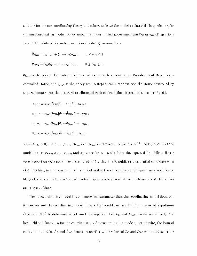
suitable for the noncoordinating theory but otherwise leave the model unchanged. In particular, for

the noncoordinating model, policy outcomes under uni�ed government are �Di or �Ri of equations

1a and 1b, while policy outcomes under divided government are

~�DRi = �D�Di + (1� �D)�Ri ; 0 � �D � 1 ;

~�RDi = �R�Ri + (1� �R)�Di ; 0 � �R � 1 :

~�DRi is the policy that voter i believes will occur with a Democratic President and Republican-

controlled House, and ~�RDi is the policy with a Republican President and the House controlled by

the Democrats. For the observed attributes of each choice de�ne, instead of equations 6a{6d,

xRRi = bNC�RRij�i � �Rijq + zRRi ;

xRDi = bNC�RDij�i � ~�RDijq + zRDi ;

xDRi = bNC�DRij�i � ~�DRijq + zDRi ;

xDDi = bNC�DDij�i � �Dijq + zDDi ;

where bNC > 0, and �RRi, �RDi, �DRi and �DDi are de�ned in Appendix A.14 The key feature of the

model is that xRRi, xRDi, xDRi, and xDDi are functions of neither the expected Republican House

vote proportion ( �Hi) nor the expected probability that the Republican presidential candidate wins

( �Pi). Nothing in the noncoordinating model makes the choice of voter i depend on the choice or

likely choice of any other voter; each voter responds solely to what each believes about the parties

and the candidates.

The noncoordinating model has one more free parameter than the coordinating model does, but

it does not nest the coordinating model. I use a likelihood-based method for non-nested hypotheses

(Dastoor 1985) to determine which model is superior. Let LC and LNC denote, respectively, the

log-likelihood functions for the coordinating and noncoordinating models, both having the form of

equation 14, and let LC and LNC denote, respectively, the values of LC and LNC computed using the

22

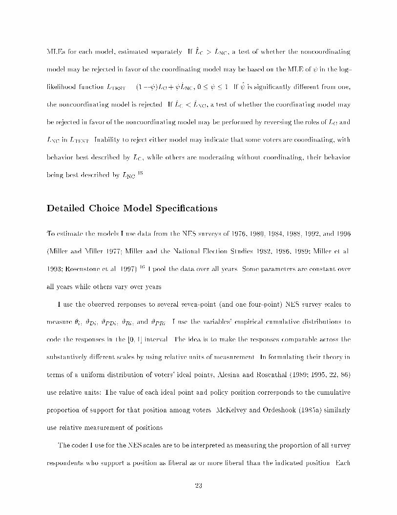
MLEs for each model, estimated separately. If LC > LNC, a test of whether the noncoordinating

model may be rejected in favor of the coordinating model may be based on the MLE of in the log-

likelihood function LTEST = (1� )LC+ LNC, 0 � � 1. If is signi�cantly di�erent from one,

the noncoordinating model is rejected. If LC < LNC, a test of whether the coordinating model may

be rejected in favor of the noncoordinating model may be performed by reversing the roles of LC and

LNC in LTEST. Inability to reject either model may indicate that some voters are coordinating, with

behavior best described by LC, while others are moderating without coordinating, their behavior

being best described by LNC.15

Detailed Choice Model Speci�cations

To estimate the models I use data from the NES surveys of 1976, 1980, 1984, 1988, 1992, and 1996

(Miller and Miller 1977; Miller and the National Election Studies 1982, 1986, 1989; Miller et al.

1993; Rosenstone et al. 1997).16 I pool the data over all years. Some parameters are constant over

all years while others vary over years.

I use the observed responses to several seven-point (and one four-point) NES survey scales to

measure �i, #Di, #PDi, #Ri, and #PRi. I use the variables' empirical cumulative distributions to

code the responses in the [0; 1] interval. The idea is to make the responses comparable across the

substantively di�erent scales by using relative units of measurement. In formulating their theory in

terms of a uniform distribution of voters' ideal points, Alesina and Rosenthal (1989; 1995, 22, 86)

use relative units: The value of each ideal point and policy position corresponds to the cumulative

proportion of support for that position among voters. McKelvey and Ordeshook (1985a) similarly

use relative measurement of positions.

The codes I use for the NES scales are to be interpreted as measuring the proportion of all survey

respondents who support a position as liberal as or more liberal than the indicated position. Each

23

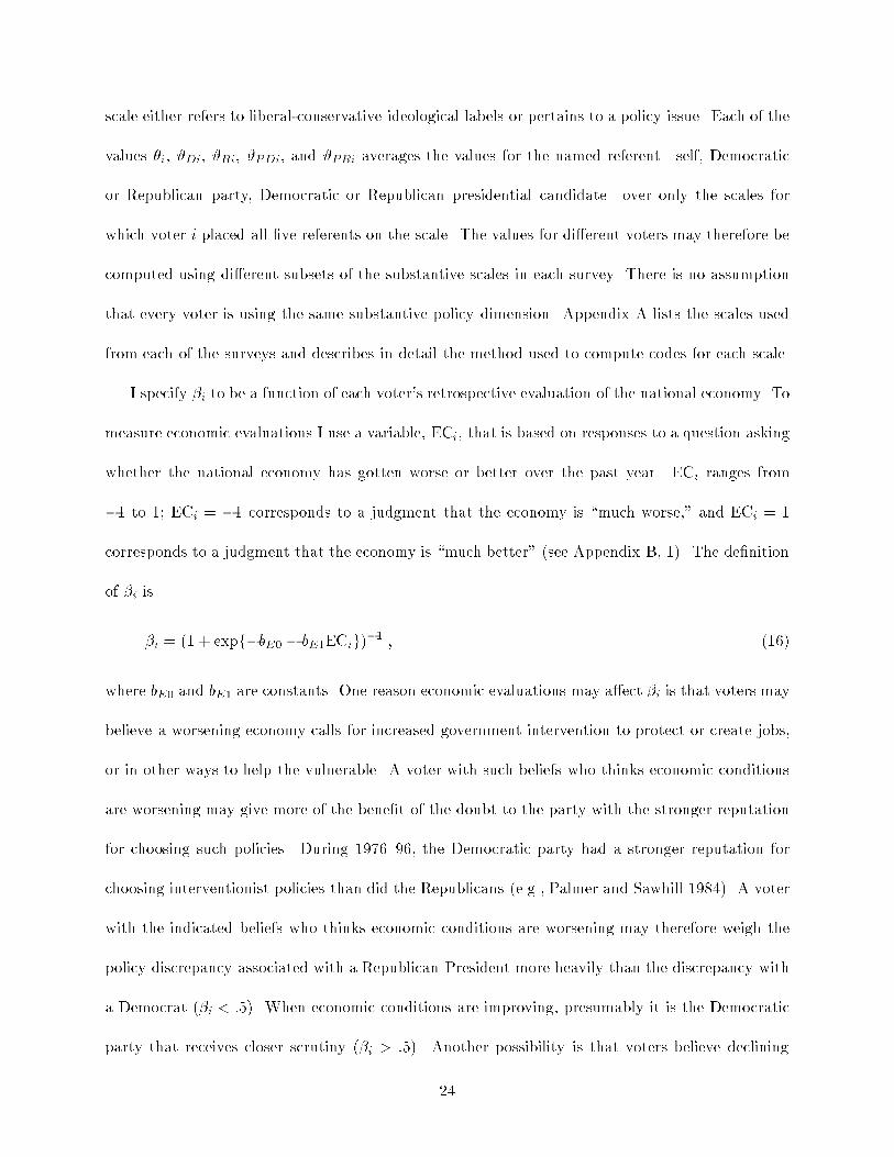
scale either refers to liberal-conservative ideological labels or pertains to a policy issue. Each of the

values �i, #Di, #Ri, #PDi, and #PRi averages the values for the named referent|self, Democratic

or Republican party, Democratic or Republican presidential candidate|over only the scales for

which voter i placed all �ve referents on the scale. The values for di�erent voters may therefore be

computed using di�erent subsets of the substantive scales in each survey. There is no assumption

that every voter is using the same substantive policy dimension. Appendix A lists the scales used

from each of the surveys and describes in detail the method used to compute codes for each scale.

I specify �i to be a function of each voter's retrospective evaluation of the national economy. To

measure economic evaluations I use a variable, ECi, that is based on responses to a question asking

whether the national economy has gotten worse or better over the past year. ECi ranges from

�1 to 1; ECi = �1 corresponds to a judgment that the economy is \much worse," and ECi = 1

corresponds to a judgment that the economy is \much better" (see Appendix B, 1). The de�nition

of �i is

�i = (1 + expf�bE0 � bE1ECig)�1 ; (16)

where bE0 and bE1 are constants. One reason economic evaluations may a�ect �i is that voters may

believe a worsening economy calls for increased government intervention to protect or create jobs,

or in other ways to help the vulnerable. A voter with such beliefs who thinks economic conditions

are worsening may give more of the bene�t of the doubt to the party with the stronger reputation

for choosing such policies. During 1976{96, the Democratic party had a stronger reputation for

choosing interventionist policies than did the Republicans (e.g., Palmer and Sawhill 1984). A voter

with the indicated beliefs who thinks economic conditions are worsening may therefore weigh the

policy discrepancy associated with a Republican President more heavily than the discrepancy with

a Democrat (�i < :5). When economic conditions are improving, presumably it is the Democratic

party that receives closer scrutiny (�i > :5). Another possibility is that voters believe declining

24

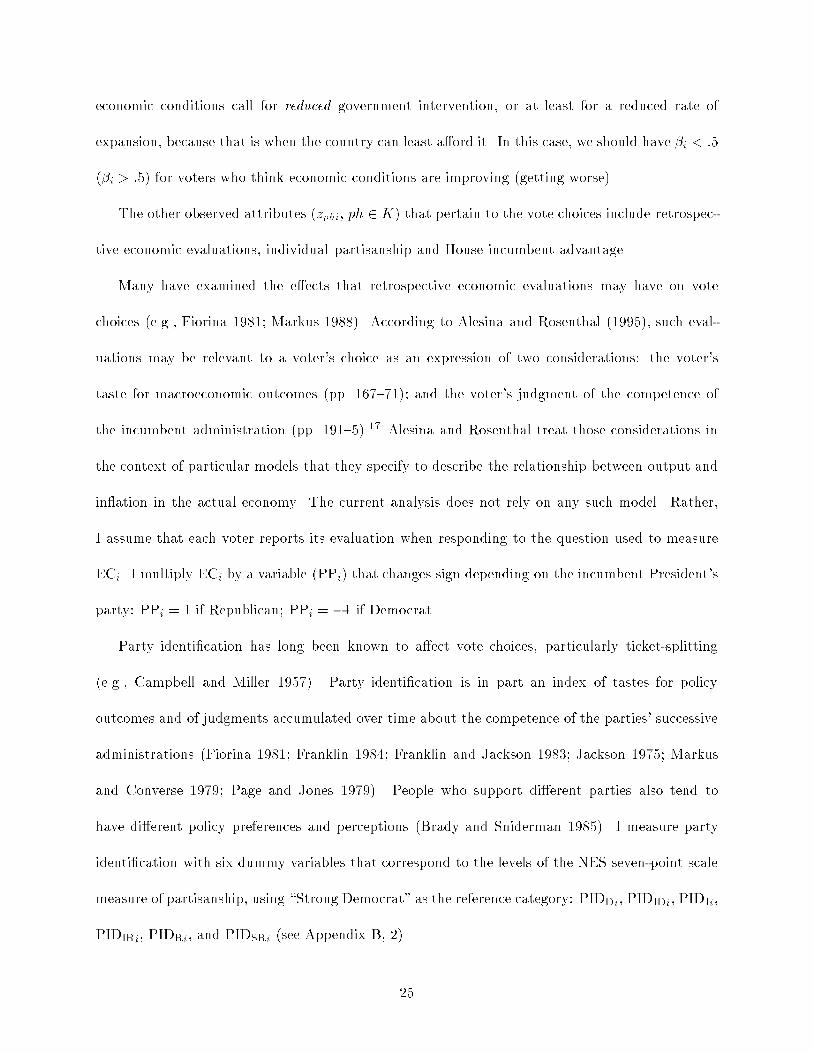
economic conditions call for reduced government intervention, or at least for a reduced rate of

expansion, because that is when the country can least a�ord it. In this case, we should have �i < :5

(�i > :5) for voters who think economic conditions are improving (getting worse).

The other observed attributes (zphi, ph 2 K) that pertain to the vote choices include retrospec-

tive economic evaluations, individual partisanship and House incumbent advantage.

Many have examined the e�ects that retrospective economic evaluations may have on vote

choices (e.g., Fiorina 1981; Markus 1988). According to Alesina and Rosenthal (1995), such eval-

uations may be relevant to a voter's choice as an expression of two considerations: the voter's

taste for macroeconomic outcomes (pp. 167{71); and the voter's judgment of the competence of

the incumbent administration (pp. 191{5).17 Alesina and Rosenthal treat those considerations in

the context of particular models that they specify to describe the relationship between output and

in ation in the actual economy. The current analysis does not rely on any such model. Rather,

I assume that each voter reports its evaluation when responding to the question used to measure

ECi. I multiply ECi by a variable (PPi) that changes sign depending on the incumbent President's

party: PPi = 1 if Republican; PPi = �1 if Democrat.

Party identi�cation has long been known to a�ect vote choices, particularly ticket-splitting

(e.g., Campbell and Miller 1957). Party identi�cation is in part an index of tastes for policy

outcomes and of judgments accumulated over time about the competence of the parties' successive

administrations (Fiorina 1981; Franklin 1984; Franklin and Jackson 1983; Jackson 1975; Markus

and Converse 1979; Page and Jones 1979). People who support di�erent parties also tend to

have di�erent policy preferences and perceptions (Brady and Sniderman 1985). I measure party

identi�cation with six dummy variables that correspond to the levels of the NES seven-point scale

measure of partisanship, using \Strong Democrat" as the reference category: PIDDi, PIDIDi, PIDIi,

PIDIRi, PIDRi, and PIDSRi (see Appendix B, 2).

25

To take incumbent advantage into account, I use a pair of dummy variables that indicate

whether a Democrat or Republican is running for reelection or whether there is an open seat:

DEMi = 1 if a Democrat is running for reelection in individual i's congressional district, otherwise

DEMi = 0; REPi = 1 if a Republican incumbent is running, otherwise REPi = 0 (see Appendix

B, 3). If DEMi = REPi = 0, then the district has an open seat. Alesina and Rosenthal (1995) use

district-level data for 1950{86 to show that midterm cycle e�ects predicted by their theory operate

pretty much independently of incumbency e�ects.18

To understand the functional form I use for zphi, ph 2 K, recall that in equations 6a{6d an

increase in xphi represents an increase in the loss voter i expects from choosing the pair of candidates

ph 2 K. Gi is speci�ed to decrease as xphi increases, via vphi = expf�xphig, ph 2 K, so that, by

equation 7, the probability that voter i chooses a candidate pair decreases if the loss expected from

choosing that pair increases. In equations 6a{6d, an increase in zphi implies an increase in xphi,

ph 2 K. So any variable that should increase the probability of choosing the candidate pair ph 2 K

and that is included with an additive e�ect in zphi should have a negative coe�cient.

The functional form for zphi, ph 2 K, is

zRRi = �cP0 � cH0 � cREPREPi � (cP1 + cH1)PPiECi

� cDPIDDi � cIDPIDIDi � cIPIDIi � cIRPIDIRi � cRPIDRi � cSRPIDSRi ; (17a)

zRDi = �cP0 + cH0 � cDEMDEMi � (cP1 � cH1)PPiECi ; (17b)

zDRi = cP0 � cH0 � cREPREPi + (cP1 � cH1)PPiECi ; (17c)

zDDi = cP0 + cH0 � cDEMDEMi + (cP1 + cH1)PPiECi

+ cDPIDDi + cIDPIDIDi + cIPIDIi + cIRPIDIRi + cRPIDRi + cSRPIDSRi ; (17d)

where cP0, cP1, cH0, and cH1 are coe�cients constant in each year, and cD, cID, cI , cIR, cR,

cSR, cDEM , and cREP are coe�cients constant over all years. Coe�cient signs should be cP0,

26

cH0 < 0 and cP1, cH1, cDEM , cREP , cD, cID, cI , cIR, cR, cSR > 0. The following examples help

understand the signs expected for the coe�cients. First, consider the e�ects of party identi�cation.

Other things equal, we expect a Strong Democrat to su�er a smaller loss from choosing Democratic

candidates than from choosing Republican candidates. Ignoring the e�ects of incumbency and

economic evaluations (that is, suppose cREP = cDEM = cP1 = cH1 = 0), that is so in equations

17a{17d for presidential candidates if cP0 < 0; in that case zDDi < zRDi and zDRi < zRRi. Likewise,

it is so for House candidates if cH0 < 0; in that case zDDi < zDRi and zRDi < zRRi. Other things

equal, a Strong Republican should experience a bigger loss from choosing a Democratic candidate

than a Strong Democrat would experience; hence, cSR > 0. In omitting separate e�ects for the

levels of party identi�cation in the speci�cations for zRDi and zDRi, I am assuming that the partisan

e�ects for presidential candidates are equal to those for House candidates, so that they cancel one

another when a voter is evaluating the split-ticket alternatives.

Next consider the e�ects of incumbency status. Other things equal, the loss from choosing

a Democratic House candidate should be smaller when that candidate is an incumbent; hence,

cDEM > 0. The motivation for cREP > 0 is analogous.

Finally, consider the e�ects of retrospective economic evaluations. If there is a Republican

President, one voter who thinks the economy has been going well and another voter who thinks

the economy has been going badly, then a simple retrospective voting hypothesis says two things.

First, other things equal, the voter who views the economy favorably should experience a smaller

loss from choosing Republican candidates than does the voter with the unfavorable view. Second,

other things equal, the voter with the more favorable view should experience a larger loss from

choosing Democratic candidates than does the other voter. If there is a Republican President, we

have PPi = 1. A voter who thinks the economy has been getting better has ECi > 0, while a voter

who thinks the economy has been getting worse has ECi < 0. If cP1 > 0, then the voter with the

27

positive view of the economy has values of zRRi and zRDi that are more negative than those of

the voter with the negative view. The voter with the positive view has values of zDRi and zDDi

that are more positive than those of the other voter. If cH1 > 0, then the values of zRRi and zDRi

are more negative for the voter with the positive view of the economy than they are for the other

voter, while the values of zRDi and zDDi are more positive for the voter with the positive view

than they are for the voter who views the economy unfavorably. With a Democratic President we

have PPi = �1, so that the orderings of the expected losses, given the voters' opinions about the

economy, are reversed.

To measure vote choices Yi (equivalently yphi, ph 2 K) I use the postelection choices reported

by individuals who said they voted (see Appendix B, 4). The sample size of voters used, pooled

over the six NES surveys, is 4,859 (by year, 1976{96, the sizes are 683, 627, 976, 719, 980, 874).

Only those who voted for either a Democrat or a Republican for both President and House seat

are included. Seven percent of such voters (386/5,245 cases) are omitted because they have data

missing due to failure to measure the policy position, economic evaluation, or party identi�cation

variables (see Appendix B, 7).

Model Estimates and Results of Tests of Coordination

The coordinating and noncoordinating models produce similar results, but the former is superior.

MLEs and standard errors (SEs) for the parameters of both models appear in Table 2.19 The coor-

dinating model estimates in Table 2 use method two (beta approximation) to compute �P . Most of

the parameters that have the same interpretation in both models have statistically indistinguish-

able estimates. The MLEs for cP1 and cH1 in each year have the correct signs for the usual kind

of retrospective voting e�ect in which candidates of the President's party lose votes among those

who think economic conditions have gotten worse, although not all the estimates are statistically

28

signi�cant. The MLEs for cP0, cH0, cD, cID, cI , cIR, cR, and cSR are appropriate for the usual

e�ects of party identi�cation|slightly larger in the noncoordinating model. The MLEs for cDEM

and cREP point to a substantial incumbent advantage, slightly larger for Republicans than for

Democrats. The function �i in the coordinating model and the corresponding functions in the

noncoordinating model imply similar patterns of sensitivity to retrospective economic evaluations

(discussed below).20 But the coordinating model log-likelihood (LC = �3186) is much greater

than that of the noncoordinating model (LNC = �3225). Using LTEST, the MLE for is = 0,

with a pro�le-likelihood 95% con�dence interval (Barndor�-Nielsen and Cox 1994, 90) of (0, .05).

The non-nested hypothesis test clearly rejects the noncoordinating model and does not reject the

coordinating model.

For every year except 1976, the coordinating voting model passes the parameter-based tests of

the conditions necessary for it to describe coordinating behavior. This entails rejecting the spatial

model that arises when �D = �R = 1. Table 3 reports the LR test statistics for the constraint

�D = �R = 1, imposed separately for each year. It is rejected in every year except 1976. The 95%

con�dence intervals shown in Table 4 support the same conclusions. Both the LR tests and the

con�dence intervals in Table 4 have been adjusted in light of the fact that four parameters have

MLEs on a boundary of the parameter space; see the discussion in Appendix A. Regarding the

other necessary conditions, 95% con�dence intervals computed as in Table 4 show q (.9, 1.1), bP

(3.1, 4.7) and bH (2.4, 8.3) to be positive and bounded well away from zero.

As the values of LC reported in Table 5 suggest, the coordinating model is superior to the nonco-

ordinating model for all four methods of computing �P . The �P values from the beta approximation

method are prima facie acceptable in the sense that �P < :5 whenever the Democratic candidate

won the presidential race and �P > :5 whenever the Republican candidate won. The normal ap-

proximation method values for �P appear intuitively to be more plausible, in that they are more

29

extreme|closer to zero or one|for years such as 1984 when prospects for one of the candidates

were widely believed to be hopeless.21 The normal approximation gives �P > :5 for 1976, however,

and using the normal approximation produces a substantially more negative value for LC, indicat-

ing a much worse �t to the data, than does the beta approximation method. Both the method

that directly uses the expected proportion of electoral votes as �P and the method that simply uses

the expected proportion of individuals' votes perform virtually as well as the beta approximation

method in terms of their LC values. Both have �P > :5 for 1976, however.22

The results in Table 5 may suggest that voters use proportions instead of probabilities in

evaluating weighted averages such as equation 3. Perhaps it would be better to think of equation 3

as representing some kind of expected bargaining outcome, which would parallel the interpretation

being applied to �Hi�Ri + (1 � �Hi)�Di as the expected position of the House, rather than as an

expected value. Or it may be, as many studies have suggested, that people do not use probability

numbers quite as formal probability theory suggests they should. Note that during the period

from September 15 to election day, the average value respondents to the 1984 NES Continuous

Monitoring Survey gave for Reagan's chance of winning was :80, a value greater than the electoral

vote proportion value ( �P = :70) but smaller than the normal approximation value ( �P = :93) (see

Appendix B, 8).

Moderation and Institutional Balancing

With expected postelection policies ~�Di and ~�Ri de�ned as in equation 2, moderation is almost

always a feature of every voter's choices in the coordinating voting model. Unless �D = �R =

1, every voter intends to produce a policy outcome that is an intermediate combination of the

parties' positions. The estimates for �H, in Table 5, show the expected position of the House,

�H�Ri + (1� �H)�Di, always to have been close to the midpoint between the parties' positions. The

30

House position was expected to be somewhat closer to the Democratic position in 1976, 1984, 1988,

and 1992, somewhat closer to the Republican position in 1996, and almost exactly at midpoint in

1980.

Such moderation, which is essentially built into the de�nitions of ~�Di and ~�Ri, has no direct

implication for the number of voters who may have been splitting their tickets to try to balance

the House position with that of the future President. One point that bears on the question of such

institutional balancing is the fact that the values of �P and �H in Table 5 are positively, not negatively,

correlated. The product-moment correlation is :09.23 One reason for the positive correlation is

suggested by the MLEs for bHP and bPH . The latter is near zero and statistically insigni�cant, but

bHP = 1:9.24 Recall that, theoretically, bHP = d �Hi=d �Pi, which should be interpreted as a relation

among mutually consistent, equilibrium pairs ( �Hi; �Pi), i = 1; : : : ; N . Indeed, given equations 11a

and 11b we have bHP = d �H=d �P , a function of the common knowledge. The positive estimate for the

derivative suggests that when the equilibrium value of �P increases, the value of �H that is mutually

consistent with it tends to increase as well: An increase in the equilibrium expected probability that

the Republican will win the presidency induces an increase in the equilibrium expected Republican

proportion of the House vote.25 In contrast, the estimate of virtually zero for bPH = d �P=d �H

suggests that an increase in the expected Republican proportion of the House vote has no e�ect on

the expected probability of a Republican presidential victory. What we have in this asymmetric

relationship between expected presidential and House voting outcomes is a presidential coattail

e�ect (Alesina and Rosenthal 1995, 104; Calvert and Ferejohn 1984; Ferejohn and Calvert 1983),

most notably a coattail e�ect that characterizes the relationship between di�erent equilibrium

election outcomes.

The positive relationship between �P and �H re ects the patterns in which changes have occurred

across election periods in ideal points, party positions, partisanship, economic evaluations, and

31

incumbency. To assess the prevalence of balancing behavior, we need to focus on the motivation

each voter has that arises solely from the policy-related components of �i;ph, ph 2 K. In the

notation of equations 6a{6d, those components are (xphi�zphi). Voter i has a policy-based incentive

to balance the House with the President (or, equivalently, the President with the House) if one of

the two split-ticket alternatives minimizes the policy-related component of the e�ect the voter's

choice has on the voter's expected loss, that is, if argminph2K(xphi � zphi) 2 fRD;DRg.

A necessary condition for voter i to have a policy-related incentive to balance is that the voter's

ideal point falls between the policy positions the voter expects the parties to act on after the

election; that is, either �Ri > �i > �Di or �Di > �i > �Ri. Table 6 shows the percentage of voters

who have such an ordering in each year in the NES data. The �gure jumps from 29% in 1976 to

45% in 1980, then varies between 43% and 52% in subsequent years. The number of voters having

a policy-related incentive to balance is therefore potentially quite large.

But only a minority of those voters who could have such an incentive, given �i, �Di and �Ri,

actually do have such an incentive once the presidential candidates' anticipated strengths in relation

to the House (�D and �R) and the expected election outcome ( �H and �P ) are taken into account.

Table 7 shows the distribution of vote choices that minimize xphi� zphi, ph 2 K, in each year. The

voters who have a policy-related incentive to balance are those for whom either xRDi � zRDi or

xDRi� zDRi is the smallest of the four values of xphi� zphi, ph 2 K. The percentage of such voters

is smaller than 20% in every year and is less than or equal to 10% in three of the six years (1980,

1988, and 1996). Such percentages match the predictions of Alesina and Rosenthal's (1995, 103)

theoretical model, in which only a small proportion of the voters who have ideal points between

the positions of the parties are predicted to split their tickets in the presidential election year.

Partisanship, economic evaluations, and incumbency frequently outweigh policy-related balanc-

ing considerations in the overall determination of whether a voter casts a split-ticket vote. Moreover,

32

the estimate for � (95% con�dence interval (.31, .47)) is large enough to suggest that a fair number

of split-ticket votes are signi�cantly motivated by other considerations that either enhance or re-

duce the appeal of both split-ticket alternatives without sharply distinguishing between them. Of

those found to have a policy-related balancing incentive in the NES data, over all years, only 31%

actually split their tickets. Only 22% of those who did not have a policy-related balancing incentive

split their tickets. The Pearson chi-squared statistic for independence in the cross-classi�cation of

split-ticket versus straight-ticket votes by split-ticket versus straight-ticket policy-related incentives

(measured by argminph2K(xphi � zphi)) is 18.8 with 1 degree of freedom, which indicates a sta-

tistically signi�cant association at any conventional test level.26 Factors that may have little or

nothing to do with a voter's policy preferences substantially a�ect the voter's choices. But both

the number of voters who have a policy-related balancing incentive and the degree to which that

incentive a�ects their choices are large enough to support a conclusion that policy-related balancing

has often been an important determinant of election outcomes.

Conclusion

Recent American elections have featured coordination among voters, based on voters' intentions to

produce postelection policy moderation between the President and the House. Inspired by policy

concerns that have been mediated through a coordination-with-moderation mechanism, a small but

signi�cant proportion of voters have been motivated to vote a split ticket in order to increase the

chances of institutional balance. Perhaps not in 1976, but in each presidential-year election from

1980 through 1996, each voter's choices between the major party candidates for President and the

House have been constrained by the anticipated election result, that is, by the aggregate result of

the choices all other voters were about to make. In recent elections the strategies and beliefs of

di�erent voters have been strongly tied together.

33

For the most part, moderation has been based on voters' expectations that the President will

be at least an equal of the House in determining postelection policy. Most of the �D and �R point

estimates are greater than :5 (see Table 2), which suggests that voters usually believe the President

to have more weight in policy outcomes than does the House. Jimmy Carter running for reelection

in 1980 is an exception (�D;80 = :4), but the most striking case of anticipating a weak President is

Bob Dole in 1996 (�R;96 = :1). One interpretation is that voters expected a Dole presidency to be

driven by the centralized and confrontational House of Speaker Newt Gingrich.

In at least one respect, the moderating mechanism has worked to the disadvantage of Democratic

candidates. The estimates for the weight variable �i (see equation 16) suggest that the Democratic

party cannot choose policies that are more extreme than those of the Republican party, without

su�ering electoral disadvantage, but the Republican party has often not been similarly restricted.

Voters who think economic conditions have worsened treat the discrepancies between their ideal

points and the policies they expect will occur with each party's President about equally: someone

who says the economy is \worse" has �i = :52, and someone who says \much worse" has �i =

:46.27 But voters who think economic conditions have improved put much more weight on the

discrepancy with a Democratic President: someone who says the economy is \better" has �i = :63,

and someone who says \much better" has �i = :69. Such a pattern is compatible with voters

treating the Democratic party more skeptically in times of prosperity, because of its interventionist

reputation, but not giving it any particular advantage when times are tough. Whatever its origin,

the asymmetric treatment of the parties means that the Democrats have had less leeway than the

Republicans to choose policy positions that are not at the center of the distribution of voters' ideal

points.

The coordinating voting model is underdeveloped in at least one crucial respect: the model says

nothing about how the equilibrium described by the �xed-point pair ( �H; �P ) and other common

34

knowledge might come about. It is unreasonable to think that voters spontaneously agree on

the equilibrium values. Indeed, it is unreasonable to believe that each voter independently keeps

track of all the information needed to de�ne and sustain an equilibrium. A coordinating voting

equilibrium can exist only if institutions exist that can aggregate and broadcast the information

everyone needs to know.

Such institutions exist. McKelvey and Ordeshook show that polls (1984, 1985a) or interest

groups and history (1985b) may support rational expectations voter equilibria even when many

voters are poorly informed. It should be possible to build such institutions directly into a model

much like the current one, with similar empirical implications but with weaker assumptions about

what each voter knows about the distribution of voters.28 More di�cult to model would be an

institution that brings everyone to agreement about the current values of the model's parameters.

Informally it is reasonable to say that this may happen during the electoral campaign, but it is

di�cult to say anything speci�c without invoking assumptions at least as strong as the direct

assumption that the parameters are common knowledge.29

On the whole, it seems reasonable to say that the equilibria here modeled with virtually no

institutional foundations are in reality sustained by a collection of institutions that may informally

be summarized as \the campaign," \polls," and \pundits." The campaign carries the processes

through which the expectations here modeled as ( �H; �P ) and the party and governmental struggles

here modeled using parameters such as �D, �R, �D, and �R converge to equilibrium values. Polls

and pundits allow each voter to monitor the expectations and struggles for power as they evolve,

without the voter having to exert much personal e�ort. To learn the candidates' chances in the

presidential race and the expected outcome in House races across the country, a voter need only

invest a little time listening to pollsters say what they think will happen. Brief attention to media

commentators may let a voter know how strong each presidential candidate may be expected to

35

be, if elected, relative to the candidate's party and to the legislature. Having so easily learned

the commonly accepted expectations for the election outcome and for the power relationships, all

a voter then needs in order to coordinate with all other voters is knowledge of the components

of the voter's own personal preferences: the voter's ideal point and what the voter thinks are the

relevant policy positions of the parties and candidates; the voter's partisanship and evaluation of

the economy; the presence or absence of an incumbent in the House race in the voter's district; and

other factors here treated as random. If su�cient institutional support exists, it is not di�cult for

voters to coordinate.

Appendix A. Proofs and Technical Measurement Issues

E�ects of Candidate Choices on a Voter's Expected Loss

Using d�i=d �Pi = d�i=d �Hi = 0, we have d�i=d �Pi = wPi + wHid �Hi=d �Pi + d�i=d �Pi and d�i=d �Hi =

wHi + wPid �Pi=d �Hi + d�i=d �Hi. The other variables used in equations equations 4a{4d are �RRi =

bPd�i=d �Pi + bHd�i=d �Hi, �RDi = bPd�i=d �Pi � bHd�i=d �Hi, �DRi = �bPd�i=d �Pi + bHd�i=d �Hi, and

�DDi = �bP d�i=d �Pi � bHd�i=d �Hi.

Probability That the Republican Wins the Presidency (Using Only Group Informa-

tion)

Let Vjk be the set and Njk = jVjkj the number of voters in State j who are members of group Vk.

�Vj =SMk=1 Vjk is the set of all voters in State j, and the total number of voters in the State is

Nj =PM

k=1Njk. Let �V(r)j denote the set of all subsets of �Vj of size r. If Zi is known for all i, then

the probability that the Republican gets a majority of the votes in State j is

�y�Pj =

PNj

r=dNj=2e

Ps2�V

(r)j

�Qi2s �i

� hQi2Vjns

(1� �i)i

PNj

r=0

Ps2�V (r)

j

�Qi2s �i

� hQi2Vjns

(1� �i)i

36

=

PNj

r=dNj=2e

Ps2�V

(r)j

QMk=1

�Qi2sjk

�i

� hQi2Vjknsjk

(1� �i)i

PNj

r=0

Ps2�V

(r)j

QMk=1

�Qi2sjk

�i

� hQi2Vjknsjk

(1� �i)i ; sjk = s \ Vjk :

The probability that the Republican candidate gets half or more of the Electoral College votes is

�P � =

PCr=C=2

Ps2C[r]

�Qj2s �y

�Pj

�hQj 62s(1� �y�Pj)

iPC

r=0

Ps2C[r]

�Qj2s �y

�Pj

�hQj 62s(1� �y�Pj)

i :

Replacing each �i in �y�Pj with the group-speci�c probability ��k , i 2 Vk, gives �P of equation 10 with

�yPj =

PNj

r=dNj=2e

Ps2�V

(r)j

QMk=1 ��

jsjk jk (1� ��k)

jVjknsjk j

PNj

r=0

Ps2�V (r)

j

QMk=1 ��

jsjkjk (1� ��k)

jVjknsjkj; sjk = s \ Vjk : (18)

Since each Zi is independent andM � N , Slutzky's theorem implies thatR~Z � � �

R~Z�P �QN

i=1 dfki(Zi)

converges in probability to �P as N ! 1 in any way such that, for every j and k, Njk ! 1 or

Njk = 0. In terms of asymptotic approximation error,

Z~Z� � �

Z~Z| {z }

N times

�P �NYi=1

dfki(Zi) = �P + Op

�max

j;k: Njk 6=0N

�1=2jk

�:

�P therefore di�ers negligibly fromR~Z � � �

R~Z�P �QN

i=1 dfki(Zi) if Njk is large for all j and k.

Existence of Fixed-Point Pairs ( �H; �P )

Let be a bounded set of positive Lebesgue measure that is the parameter space for �i;ph, ph 2 K.30

Let ��k`| and ��k`| denote the values of ��k and ��k when evaluated using �P = ` and �H = | for some

` 2 [0; 1] and some | 2 [0; 1]. Let �P`| denote the value of �P as de�ned by equation 10 when

��k = ��k`|, and let �H`| denote the value of �H as de�ned by equation 9 when ��k = ��k`|.

Theorem 2 For almost every 2 , there exist values `; | 2 (0; 1) such that, simultaneously,

�P`| = ` and �H`| = |.

Because ��k`| varies continuously as a function of ` for each k and �P`| is a continuous function of

the ��k`| values, there is at least one �xed point of �P`| as a function of ` for each �xed value of |,

37

that is, there is at least one value ` such that �P`| = `. Because �P0| > 0 and �P1| < 1, the number

of �xed points is odd, except on a subset of of measure zero. For q > 1 there is similarly an odd

number of �xed points �H`| = | for each `. If q = 1, the step functions in wHi imply that �H`| does

not vary continuously as a function of |, so if q = 1 there is not necessarily a �xed point �H`| = |.

If 0 < q < 1, then there is a discontinuity at in�nity in wHi whenever �i = ~�Di or �i = ~�Ri. But for

a �nite number N of voters, the number of points of discontinuity in both cases is �nite.31 So the

values of ` for which there is no �xed point �H`| = | form a set of measure zero: for any � > 0 there

is a value `0, j`� `0j < �, such that there is a �xed point �H`0| = | for some | 2 [0; 1]. Now consider

the graph of the set of �xed points �P`| = ` as | varies over [0; 1] and the graph of the set of �xed

points �H`| = | as ` varies over [0; 1]. When q > 1 both graphs are continuous and so necessarily

intersect. That is, there is necessarily at least one pair of values (`; |) such that �P`| = ` and �H`| = |.

If 0 < q � 1, then each graph is in general not continuous, because of the discontinuities in wHi,

but each graph does have a �nite number of continuous components. In this case, the graphs need

not intersect. But because the number of points of discontinuity is �nite, the set of parameter

values for which there is no intersection has measure zero. For �nite N > 0, the argument holds

for arbitrary �nite sets of probability measures fk . Q.E.D.

Survey-based Probabilities That the Republican Wins the Presidency ( �P )

Let CNR denote the number of electoral votes assigned to the Republican according to the �vj = ;

convention, and let CND denote the number thus assigned to the Democrat. The proportion of the

remaining electoral votes that the Republican needs to win is �� = (269�CNR)=(538�CNR�CND).

Beta approximation method. For States with sample data, set �yPj = yPj . Compute the variance of

�R as �2�R = (PS

j=1 C2j )

�1PSj=1 �yPj(1� �yPj)C

2j . To evaluate Pr(�R > :5), use the beta distribution

38

on [0; 1] obtained by matching moments:

�P =

Z 1

��

�p1�1R (1� �R)p2�1

B(p1; p2)d�R ; (19)

where p1 = ��2R(1 ���R)=�

2�R� ��R and p2 = ��R(1 � ��R)

2=�2�R � (1 � ��R) match the mean ��R and

variance �2�R (Johnson, Kotz, and Balakrishnan 1995, 222), and B(p1; p2) denotes the beta function.

If p1 � 0 or p2 � 0, then the beta distribution is inappropriate. Normal approximation method.

Set �yPj = 1� �((:5� yPj)=�yPj) and evaluate Pr(�R > :5) as �P = 1� �((�� � ��R)=��R).

Iterative Computation of MLEs and Expectations ( �H; �P)

Given estimates for the parameters and estimates �H({) and �P ({) from iteration step {, use equation

7 to compute probability values �({)phi, ph 2 K, and then �

({)i and �

({)i for each voter. For each

State j with �vj 6= ; in the referent year, use equation 13 to compute y({)Pj and hence compute an

updated estimate �P ({+1) (e.g., using mean ��({)R , variance �

2({)�R

and equation 19). Use equation 12

to estimate �H({+1), with n being the total sample size of voters for the referent year. Use �H({+1)

and �P ({+1) and the parameter values of step { to apply one step of Gauss-Newton maximization

to the log-likelihood, in order to get new parameter values for use in iteration {+ 1. Iterate until,

for successive iterations { and { + 1, ( �H({); �P ({)) = ( �H({+1); �P ({+1)) and the parameter estimates

satisfy the �rst- and second-order conditions for a local maximum of the log-likelihood. In each

Gauss-Newton step, each row of the Jacobian matrix of the parameters is weighted by 1=!i.32 1=!i

is scaled to sum to the total sample size ~n in each year, where ~n includes all survey respondents,

both voters and nonvoters (see Appendix B, 5).

For a �xed set of parameter estimates, the sequence ( �H(1); �P (1)); ( �H(2); �P (2)); : : : converges if,

to extend the notation of the paragraph on the existence of �xed-point pairs, �P `| is decreasing in

| and �H`| is decreasing in ` for |; ` 2 (0; 1).

39

Estimates on a Boundary of the Parameter Space

Table 2 shows �D;76, �D;92, �R;80, and �R;96 to have MLEs equal to 1:0, on the conceptual boundary

of the parameter space. The boundary is not a \natural" boundary (Moran 1971b) for the probabil-

ity model: LC is a proper (although meaningless) likelihood for values of �D, �D, or �R outside [0; 1].

The on-boundary values do not imply problems with the consistency of the MLEs (Moran 1971a):

The model is identi�ed and the MLEs globally maximize LC subject to 0 � �D; �R; �D; �R � 1.

But the MLEs' asymptotic distribution is complicated (Moran 1971b; Self and Liang 1987). To

regularize the model for the LR tests, in all the constrained models I �x equal to 1:0 the parameters

with on-boundary MLEs. With this method the test statistic for �D;76 = �R;76 = 1 has only one

degree of freedom. None of the statistics in Table 3 are close to the critical value for a test based

on �22 (�21 for 1976), so slight variations from �22 in the statistics' distributions would not change

any conclusions. Unfortunately, it is computationally infeasible to bootstrap the LR test statistics.

The asymptotic distribution of the MLEs when parameters fall on a boundary of the parameter

space is a mixture of censored multivariate normal distributions (Moran 1971b; Self and Liang 1987).

For the coordinating voting model, the hypothesis �D;76 = �D;92 = �R;80 = �R;96 = 1 implies a

distribution that is a mixture of 16 censored distributions. I use a bootstrap (20,000 resamples) of

the score vectors associated with the MLEs of Table 2 to tabulate that mixture distribution and

estimate the con�dence intervals of Table 4. With a few substantial exceptions (e.g., �R;88) the

con�dence intervals do not di�er greatly from the intervals obtained by using normal theory with

the MLEs and SEs in Table 2 (i.e., MLE � 1:96 SE).

40

Comparison Weights in the Noncoordinating Vote Choice Model

The weight of the spatial comparison associated with each form of government is

�ji =expf�bjE0 � bjE1ECig

1 +P

j02fRR;RD;DRg expf�bj0E0 � bj0E1ECig; j 2 fRR;RD;DRg

�DDi = 1� �RRi � �RDi � �DRi

for coe�cients bjE0, bjE1, j 2 fRR;RD;DRg. See the text preceding equation 16 for the de�nition

of ECi. If all forms of government are treated symmetrically, �RRi = �RDi = �DRi = �DDi =14 .

Measuring Ideal Points and Policy Positions

To measure �i, #Di, #PDi, #Ri, and #PRi, I use a collection of sets of �ve seven-point (and one set

of �ve four-point) placement scales. Each set includes one scale for self, one for each party, and

one for each presidential candidate, all referring to the same substantive policy description (see

Appendix B, 6). All scale items are oriented so that the \liberal" position during the given time

period has the lower number.

The general motivation for the response codes is the observation that any continuous random

variable X can be mapped onto a scale such that the values of the scale have probability mass

spread uniformly over [0; 1]. Simply map each value x of the variable to the value of the variable's

distribution function, FX(x) = Pr(X < x). If X is multivariate with components X1; : : : ; Xk,

then the mapping from vectors (x1; : : : ; xk) to a uniform distribution on [0; 1] may be based on

the distribution function FX(x) = Pr(X1 < x1; : : : ; Xk < xk). I do not try to estimate the joint,

�ve-dimensional distribution function for the �ve scales of each substantive description. Rather I

crudely approximate the joint distribution by computing the simple average of the observed one-

dimensional marginal distributions.

To assign a code in the [0; 1] interval to the response levels of each scale, I �rst compute the

41

cumulative response proportions for the �ve scales in the set for each substantive description. Let

0 = rsj0 � rsj1 � � � � � rsj6 � rsj7 = 1 denote the successive cumulative proportions for substantive

description s (e.g., s = \Liberal/Conservative") and scale j 2 fS;D;R; PD;PRg, S = self, D =

Democratic party, R = Republican party, PD = Democratic candidate, and PR = Republican

candidate. For each m 2 f0; : : : ; 7g, I compute rsm = (rsSm + rsDm + rsRm + rsPDm + rsPRm)=5.

For all �ve scales of type s, the numerical code used for original response category m 2 f1; : : : ; 7g

is �rsm = (rs;m�1 + rsm)=2. To determine values for �i, #Di, #PDi, #Ri, and #PRi for each voter, I

average the score for the corresponding scale j over all (and only) the substantive descriptions for

which the person responded to all �ve scales for that substantive description.

Appendix B. Data Notes

1. Economic Evaluations (ECi). For 1976 the question wording is: \Would you say that at the

present time business conditions are better or worse than they were a year ago?" For 1980, 1984,

and 1988 the question wording is: \What about the economy? Would you say that over the past

year the nation's economy has gotten better, stayed about the same, or gotten worse?" For 1992

the initial part of the question was changed to read: \How about the economy." For 1996 the initial

part was: \Now thinking about the economy in the country as a whole." For all years except 1976,

the responses are coded \much worse" (�1), \somewhat worse" (�:5), \same" (0), \somewhat

better" (.5), and \better" (1). For 1976 only three levels of response were recorded, coded here as

\worse now" (�:5), \about the same" (0), and \better now" (.5). The NES variable numbers for

each year are 3139 (1976), 150 (1980), 228 (1984), 244 (1988), 3532 (1992), and 960386 (1996).

2. Party Identi�cation (PIDDi, PIDIDi, PIDIi, PIDIRi, PIDRi, PIDSRi). The levels of the

party identi�cation scale are Strong Democrat, Democrat, Independent Democratic, Independent,

Independent Republican, Republican, and Strong Republican. The variable numbers are 3174

42

(1976), 266 (1980), 866 (1984), 274 (1988), 3634 (1992), and 960420 (1996).

3. Incumbency Status (DEMi, REPi). For 1976, incumbency status variables were built from

note 17 in the codebook �le nes1976.cbk. The variable numbers for the other years are 740 (1980), 59

(1984), 50 (1988), 3021 (1992; with errors corrected as indicated in the codebook �le nes92int.cbk),

and 960097 (1996).

4. Vote Choices (yphi). The variable numbers are 3665 and 3673 (1976), 994 and 998 (1980),

788 and 793 (1984), 763 and 768 (1988), 5609 and 5623 (1992), and 961082 and 961089 (1996).

5. Sampling Weights (1=!i). In the NES data, 1=!i is the number of adults in each household,

which is multiplied by a time-series weight in years (1976, 1992, 1996) when part of the sample

belonged to a multiyear panel cohort. I rescaled the number of adults and time-series weight

variables to give each a mean of 1.0 over the whole of each survey sample. The variable numbers

are 3003 and 3021 (1976); 43 (1980); 70 (1984); 91 (1988); 29, 3076, and 7000 (1992); and 960046A

and 960005 (1996).

6. Placement Scales (�i, #Di, #PDi, #Ri, #PRi). Here are the brief substantive description

and variable numbers for each set of scales for each year. The label \reversed" indicates an item

whose categories were reordered to reverse the original ordering of 1 to 7 (or for Abortion in

1996, 1 to 4). 1976: Government Guaranteed Job and Living Standard, 3241{5; Rights of the

Accused, 3248{52; School Busing to Achieve Integration, 3257{61; Government Aid to Minori-

ties, 3264{8; Government Medical Insurance Plan, 3273{7; Liberal/Conservative Views, 3286{90;

Government Guaranteed Job and Living Standard, 3758{62; Urban Unrest, 3767{71; Legaliza-

tion of Marijuana, 3772{6; Change in Tax Rate, 3779{83; and Equal Rights for Women, 3787{91.

1980: Liberal/Conservative, 267{9, 278, 279; Defense Spending, 281{3, 286, 287; Government Ser-

vices/Spending (reversed), 291{3, 296, 297; Reduce In ation/Reduce Unemployment (reversed),

301{3, 306, 307; Liberal/Conservative Views, 1037{9, 1053, 1054; Government Aid to Minorities,

43

1062{4, 1073, 1074; Getting Along with Russia, 1078{80, 1089, 1090; Equal Rights for Women,

1094{6, 1105, 1106; and Government Guaranteed Job and Living Standard, 1110{2, 1121, 1122.

1984: Liberal/Conservative Placement, 119{21, 123{5, 127{9, 131{3, 135{7; Liberal/Conservative,

369, 371{4; Government Services/Spending (reversed), 375{9; Minority Aid/No Aid, 382{6; In-

volvement in Central America (reversed), 388{92; Defense Spending, 395{9; Social/Economic Sta-

tus of Women, 401{5; Cooperation with Russia, 408{12; and Guaranteed Standard of Living/Job,

414{8. 1988: Liberal/Conservative, 228, 231, 232, 234, 235; Government Services/Spending (re-

versed), 302{4, 307, 308; Defense Spending, 310{2, 315, 316; Government-Funded Insurance, 318{

22; Guaranteed Standard of Living/Job, 323{5, 328, 329; Social/Economic Status of Blacks, 332{4,

337, 338; Social/Economic Status of Minorities, 340{2, 345, 346; Cooperation with Russia, 368{70,

373, 374; and Women's Rights, 387{91. 1992: Ideological Placement, 3509, 3514, 3515, 3517,

3518; Government Services/Spending (reversed), 3701{5; Defense Spending, 3707{11; and Job As-

surance, 3718{22. 1996 (omitting the variable number pre�x 960): Liberal/Conservative, 365, 369,

371, 379, 380; Government Services/Spending (reversed), 450, 453, 455, 461, 462; Defense Spend-

ing, 463, 466, 469, 477, 478; Abortion (reversed), 503, 506, 509, 517, 518; Jobs/Environment, 523,

526, 529, 535, 536; and Environmental Regulation, 537, 538, 539, 541, 542.

7. Missing Data. The loss of cases from ignoring third-party votes substantially a�ects only

presidential votes. Among the 7,198 cases in which any vote cast was for a Democrat or a Repub-

lican, 1,426 cast a vote for only one o�ce (either President or House member). Among the 5,772

who said they voted for Democratic or Republican candidates for both o�ces, 527 were excluded

because the incumbent in their district was unopposed. Of the remaining cases, 379 were missing

data for the ideal point, policy positions or economic evaluation (295 missing only one or more

position variables, 58 missing only ECi, 26 missing both); seven more cases were missing data for

party identi�cation.

44

8. Reagan's Chance of Winning . The Continuous Monitoring Survey is Miller and the National

Election Studies (1985). The item wording (var. 1001) is: \As you know, Ronald Reagan has

been nominated by the Republican party. What chance do you think he has of winning the 1984

Presidential election? We will use a scale that goes from 0 to 100 where 0 represents NO chance

of winning the Presidency, 50 represents an even chance, and 100 represents certain victory." In

computing the mean I weighted observations in proportion to the number of adults (var. 16) and

in inverse proportion to the number of nonbusiness telephones (vars. 1129, 1131, 1133) in the

household. The text reports the mean divided by 100.

45

Notes

Walter R. Mebane, Jr., is Associate Professor of Government, Cornell University, Ithaca, NY 14853-

4601 (email wrm1@cornell.edu).

Earlier versions of this paper were presented at the 1998 Summer Methods Conference, Univer-

sity of California, San Diego, July 23{26; 1998 annual meeting of the Midwest Political Science As-

sociation, April 23{25, Chicago, IL; and 1997 Summer Methods Conference, Ohio State University,

Columbus, July 24{27. I worked on the paper while visiting during fall 1997 at the Department of

Social and Decision Sciences at Carnegie Mellon University, at the invitation of Bill Keech. I thank

Jasjeet Sekhon, Jonathan Wand, Jonathan Cowden, and Matthew Wexler for helpful comments,

Jonathan Cowden and Jasjeet Sekhon for letting tron and lapo help macht with the computing, and

Jonathan Ho�man for assistance in preparing the �nal copy of the manuscript. Data were made

available in part by the Cornell Institute for Social and Economic Research and the Inter-University

Consortium for Political and Social Research. All errors are solely the responsibility of the author.

1. Studies of electoral coordination often focus on the \wasted vote" logic of Duverger's Law,

which is said to keep the number of parties receiving votes small (e.g., Cox 1997; Fey 1997; Palfrey

1989). I examine coordination that relates not to the number of parties|two are assumed|but to

possible moderation in voting for President and the House of Representatives.

2. McKelvey and Ordeshook's (1984, 1985a, 1985b) equilibrium concepts are similar in that they

use rational expectations, but they di�er technically because their models feature purely spatial

utility rather than probabilistic voting, assume the existence of a single policy dimension (although

some voters are uninformed about candidates' positions), and have each voter voting for only one

o�ce rather than two. Enelow and Hinich's (1982, 1983a, 1983b) probabilistic vote choice models

also emphasize voters' expectations regarding other voters' votes.

3. See especially note 28.

46

4. Let �i;R denote voter i's loss if i chooses the Republican candidate, and let �i;D denote the

loss if i chooses the Democrat. Obviously, �i;R � �i;D = ( �Pi;R � �Pi;D)(�i;R� �i;D)=( �Pi;R� �Pi;D), if

�Pi;R � �Pi;D > 0. But if �Pi;R � �Pi;D is very small, then (�i;R � �i;D)=( �Pi;R � �Pi;D) � d�i=d �Pi.

5. Strictly speaking, to de�ne �Pi with reference to the Electoral College, I will assume that the

number of voters in each of the M groups in each State is common knowledge.

6. See Maddala 1983 for an introductory discussion of GEV choice models.

7. It is possible to specify GEV distributions in which there is also dependence among all the

pairs that include a candidate from one party. That is, �RRi, �RDi, and �DRi are dependent, or �RDi,

�DRi, and �DDi are dependent. In an analysis reported in Mebane 1998, using the same NES data,

tests show neither party-based pattern of dependence to be present, as long as party identi�cation

is included among the variables in (zRRi; zRDi; zDRi; zDDi). Given those empirical results, I simplify

the current model by ignoring the possibility of party-based dependence.

8. To accommodate the combination of continuous and discrete variables that Zi may contain,

the integral in Pr(Yi = ph j i 2 Vk) may be thought of as a Riemann-Stieltjes, or if necessary

Lebesgue-Stieltjes, integral (Billingsley 1986, 230).

9. �P is the expected probability that the Republican wins or ties in the Electoral College. I

ignore the complications involved in breaking a tie by votes in the House.

10. An exact tie between two �i;ph values, ph 2 K, is a measure zero event that may be ignored.

11. Let f� denote the density of �i on R4 (the real line four times). The basic result is

Z~Z

ZR4(~�phi � ��phki)df�(�i)dfki(Zi)

=

Z~Z

ZR4

~�phidf�(�i)dfki(Zi)� ��phki

Z~Z

ZR4df�(�i)dfki(Zi)

=

Z~Z�phidfki(Zi)� ��phki = 0 ; ph 2 K; i = 1; : : : ; N :

We have immediately that N�1PNi=1

R~Z

RR4(~�i� ��ki)=Ndf�(�i)dfk(Zi) = 0 and, by Slutzsky's theo-

47

rem based on the continuity of gi and usingM � N ,N�1PN

i=1

R~Z

RR4 gi(~�i���ki)df�(�i)dfk(Zi)

Pr! 0.

12. Isaki and Fuller (1982) rigorously develop the relevant concept of consistency. See S�arndal,

Swensson, and Wretman (1992, 166{85) for an overview.

13. If var(�phi) =16�

2�2, ph 2 K (see Johnson, Kotz and Balakrishnan 1995, 12), then the

estimated parameters correspond to bP = �Pi;R � �Pi;D and bH = �Hi;R � �Hi;D divided by �.

14. Born's (1994a) implementation of Fiorina's theory is similar to the noncoordinating model,

the di�erences being that Born constrains �D = �R; assumes uncorrelated disturbances (� = 0);

�xes q = 1; uses a single, constant parameter for each of the coe�cients here allowed to vary over

voters via bNC�phi, ph 2 K; measures ideal points and policy positions di�erently; and includes

in zphi variables to measure \Evaluation of President's Job Performance" but not retrospective

economic evaluations. Born does not estimate the �R = �D parameter simultaneously with the

rest of his model but instead repeatedly reestimates the model for several values in the range .5 to

.85.

15. Ingberman and Villani (1993) study a model in which there are both strategic and non-

strategic voters.

16. Data and documentation for 1976{92 are from the \ANES 1948{1994 CD-ROM" of May

1995 (ICPSR CD0010). Data and documentation for 1996 were obtained by ftp from ICPSR in

June 1997.

17. Alesina, Roubini, and Cohen (1997) further review \rational retrospective voting" models.

18. The district-level analysis is subject to ecological inference biases.

19. Estimates were computed using SAS, PROC NLIN (SAS Institute 1989{95), with numerical

derivatives. Over all years, the percentage correctly classi�ed by \predicting" for each observation

the pair of vote choices that has the highest probability using the parameter MLEs is 73.6% (by

year: 68.7%, 67.0%, 74.4%, 75.9%, 74.6%, 78.3%). Over all years the average probability of the

48

pair of choices actually made is .64 (by year: .58, .58, .65, .66, .65, .69).

20. Indeed, using the MLEs for each model, �i = �DRi + �DDi.

21. The estimates from the normal approximation method are numerically the closest to the

more extreme values that Alesina, Roubini, and Cohen (1997, 114{20, 135{7) obtain by using the

statistics of a Brownian motion (running in reverse) to model sequences of Gallup poll results.

A key assumption of the Brownian motion model, that the di�erences between successive polls

are independent, is incompatible with the idea that the sequence of polls informs voters about

the aggregate distribution of voters' preferences, and therefore it is incompatible with convergence

results such as McKelvey and Ordeshook (1985a) and Nielsen et al. (1990) discuss.

22. Except for 1976, the simple vote proportions in Table 5 have values somewhat more extreme

than the actual Republican proportion of the two-party popular vote, re ecting the overreporting of

votes for the winner that occurs in NES postelection data. In order by year, the actual proportions

are .489, .553, .592, .539, .465, and .453 (Miller 1997).

23. With 1996 omitted, the correlation is :85. These correlations are for the beta approximation

value of �P . Results for the other methods are similar.

24. The 95% con�dence interval for bHP , computed as in Table 4, is (.9, 2.8).

25. It is important to keep clear that bHP refers to local variations among equilibria. Numerical

computations using the NES data and the parameter MLEs of Table 2 show that @ �P `|=@| < 0 and

@ �H`|=@` < 0 for `; | 2 (0; 1). Moreover, the values �P `| = ` are decreasing in |, and the values

�H`| = | are decreasing in ` for `; | 2 (0; 1) (see Appendix A for the `; | notation). The assumption

of global linearity that bHP = d �H=d �P re ects is restrictive.

26. Overall, the coordinating voting model does not do especially well in classifying split-ticket

voters separately from straight-ticket voters. Of the 597 voters \predicted" to split their tickets,

48% did so; of the 1,101 voters who split their tickets, only 26% were \predicted" to do so.

49

27. The values for �i are computed using the MLEs for bE0 and bE1.

28. For instance, suppose the decision rule of equation 5 is common knowledge, but no voter

knows the distribution of other voters' preferences, that is, no one knows the probability measures

fk or the distribution FPH . If the unknown distributions are such that @ �P`|=@| < 0 and @ �H`|=@` < 0

for `; | 2 (0; 1), then a sequence of preelection polls will converge to a �xed point ( �H; �P ). Nielsen

et al. (1990) discuss convergence for a scalar aggregate statistic. To achieve convergence to a

neighborhood of ( �H; �P ), it is not necessary for every voter to learn the result of every poll, nor

for every voter to have the same probability of learning about each poll. If under the common

knowledge assumptions of the current model the �xed point ( �H; �P ) would be unique and stable for

the given population of voters, and if each voter has a positive probability of learning about each

poll and updates consistently, then Bowden's (1987) results imply that aggregate pre-election poll

results evolve according to a Markov process that converges to a stationary distribution with mean

( �H; �P ). It seems obvious that if each voter uses Bayesian updating based on a suitable likelihood,

then the mode of the distribution of each voter's beliefs converges over time to ( �H; �P ) (cf. McKelvey

and Page 1990). The process may not converge by the time of any particular election, however.

29. For instance, at least as strong would be an assumption that all voters have a common

knowledge prior distribution for the parameters, from which they then update based on public

campaign information.

30. Con�ne �D; �R 2 [0; 1). As discussed in the text, �D = �R = 1 is incompatible with

coordination.

31. If the ideal point and policy position variables are continuous, then the set of discontinuities

has measure zero.

32. In PROC NLIN I used WEIGHT to weight the Jacobian matrix (SAS Institute 1990, 1148).

50

References

Alesina, Alberto, John Londregan and Howard Rosenthal. 1993. \A Model of the Political

Economy of the United States." American Political Science Review 87 (March): 12{33.

Alesina, Alberto, and Howard Rosenthal. 1989. \Partisan Cycles in Congressional Elections and

the Macroeconomy." American Political Science Review 83 (June): 373{98.

Alesina, Alberto, and Howard Rosenthal. 1995. Partisan Politics, Divided Government, and the

Economy. New York: Cambridge University Press.

Alesina, Alberto, and Howard Rosenthal. 1996. \A Theory of Divided Government." Economet-

rica 64 (November): 1311{41.

Alesina, Alberto, Nouriel Roubini and Gerald D. Cohen. 1997. Political Cycles and the Macroe-

conomy. Cambridge, MA: MIT Press.

Alvarez, R. Michael, and Matthew M. Schousen. 1993. \Policy Moderation of Con icting Expec-

tations: Testing the Intentional Models of Split-ticket Voting." American Politics Quarterly

21 (4): 410{38.

Aumann, Robert J. 1976. \Agreeing to Disagree." Annals of Statistics 4 (November): 1236{9.

Barndor�-Nielsen, O. E., and D. R. Cox. 1994. Inference and Asymptotics. London: Chapman

and Hall.

Billingsley, Patrick. 1986. Probability and Measure. 2d ed. New York: Wiley.

Born, Richard. 1994a. \Split-ticket Voters, Divided Government and Fiorina's Policy-balancing

Model." Legislative Studies Quarterly 19 (1): 95{115.

Born, Richard. 1994b. \Rejoinder." Legislative Studies Quarterly 19 (1): 126{9.

51

B�orsch-Supan, Axel. 1990. \On the Compatibility of Nested Logit Models with Utility Maximiza-

tion." Journal of Econometrics 43 (March): 373{88.

Bowden, Roger J. 1987. \Repeated Sampling in the Presence of Publication E�ects." Journal of

the American Statistical Association 82 (June): 476{84.

Brady, Henry, and Paul M. Sniderman. 1985. \Attitude Attribution: A Group Basis for Political

Reasoning." American Political Science Review 79 (December): 1061{78.

Burden, Barry C., and David C. Kimball. 1998. \A New Approach to the Study of Ticket

Splitting." American Political Science Review 92 (September): 533{44.

Calvert, Randall L., and John A. Ferejohn. 1983. \Coattail Voting in Recent Presidential Elec-

tions." American Political Science Review 77 (June): 407{19.

Campbell, Angus, and Warren E. Miller. 1957. \The Motivational Basis of Straight and Split

Ticket Voting." American Political Science Review 51 (June): 293{312.

Cox, Gary W. 1997. Making Votes Count: Strategic Coordination in the World's Electoral Sys-

tems. New York: Cambridge University Press.

Dastoor, Naorayex K. 1985. \A Classical Approach to Cox's Test for Non-nested Hypotheses."

Journal of Econometrics 27 (March): 363{70.

Enelow, James C., and Melvin J. Hinich. 1982. \Ideology, Issues, and the Spatial Theory of

Elections." American Political Science Review 76 (September): 493{501.

Enelow, James C., and Melvin J. Hinich. 1983a. \Voting One Issue at a Time: The Question of

Voter Forecasts." American Political Science Review 77 (June): 435{45.

52

Enelow, James C., and Melvin J. Hinich. 1983b. \Voter Expectations in Multi-Stage Voting

Systems: An Equilibrium Result." American Journal of Political Science 27 (November):

820{7.

Ferejohn, John A., and Randall L. Calvert. 1983. \Presidential Coattails in Historical Perspec-

tive." American Journal of Political Science 28 (February): 127{46.

Fey, Mark. 1997. \Stability and Coordination in Duverger's Law: A Formal Model of Preelection

Polls and Strategic Voting." American Political Science Review 91 (March): 135{47.

Fiorina, Morris P. 1981. Retrospective Voting in American National Elections. New Haven, CT:

Yale University Press.

Fiorina, Morris P. 1988. \The Reagan Years: Turning to the Right or Groping Toward the

Middle." In The Resurgence of Conservatism in Anglo-American Democracies, ed. Barry

Cooper, Allan Kornberg, and William Mishler. Durham, NC: Duke University Press. Pp.

430{59.

Fiorina, Morris P. 1992. Divided Government. New York: Macmillan.

Fiorina, Morris P. 1994. \Response to Born." Legislative Studies Quarterly 19 (1): 117{25.

Franklin, Charles H. 1984. \Issue Preferences, Socialization, and the Evolution of Party Identi�-

cation." American Journal of Political Science 28 (August): 459{78.

Franklin, Charles H., and John E. Jackson. 1983. \The Dynamics of Party Identi�cation."

American Political Science Review 77 (December): 957{73.

Frymer, Paul. 1994. \Ideological Consensus within Divided Government." Political Science

Quarterly 109 (2): 287{311.

53

Fudenberg, Drew, and Jean Tirole. 1991. Game Theory. Cambridge, MA: MIT Press.

Galambos, Janos. 1987. The Asymptotic Theory of Extreme Order Statistics. 2d ed. Malabar,

FL: Robert E. Krieger.

Grossman, Sanford J. 1989. The Informational Role of Prices. Cambridge, MA: MIT Press.

Ingberman, Daniel, and John Villani. 1993. \An Institutional Theory of Divided Government

and Party Polarization." American Journal of Political Science 37 (May): 429{71.

Isaki, Cary T., and Wayne A. Fuller. 1982. \Survey Design Under the Regression Superpopulation

Model." Journal of the American Statistical Association 77 (March): 89{96.

Jackson, John E. 1975. \Issues, Party Choices and Presidential Votes." American Journal of

Political Science 19 (May): 161{85.

Johnson, Norman L., Samuel Kotz and N. Balakrishnan. 1995. Continuous Univariate Distribu-

tions, Volume 2. 2d ed. New York: John Wiley & Sons.

Kreps, David M. 1977. \A Note on `Ful�lled Expectations' Equilibria." Journal of Economic

Theory 14 (February): 32{43.

Maddala, G. S. 1983. Limited-dependent and Qualitative Variables in Econometrics. New York:

Cambridge University Press.

Markus, Gregory B. 1988. \The Impact of Personal and National Economic Conditions on the

Presidential Vote: A Pooled Cross-Sectional Analysis." American Journal of Political Science

32 (February): 137{54.

Markus, Gregory B., and Philip E. Converse. 1979. \A Dynamic Simultaneous Equation Model

of Electoral Choice." American Political Science Review 73 (December): 1055{70.

54

McFadden, Daniel. 1978. \Modelling the Choice of Residential Location." In Spatial Interaction

Theory and Planning Models, ed. Anders Karlqvist, Lars Lundqvist, Folke Snickars and J�orgen

W. Weibull. New York: North-Holland. Pp. 75{96.

McKelvey, Richard D., and Peter C. Ordeshook. 1984. \Rational Expectations in Elections: Some

Experimental Results Based on a Multidimensional Model." Public Choice 44 (1): 61{102.

McKelvey, Richard D., and Peter C. Ordeshook. 1985a. \Elections with Limited Information: A

Ful�lled Expectations Model Using Contemporaneous Poll and Endorsement Data as Infor-

mation Sources." Journal of Economic Theory 36 (June): 55{85.

McKelvey, Richard D., and Peter C. Ordeshook. 1985b. \Sequential Elections with Limited

Information." American Journal of Political Science 29 (August): 480{512.

McKelvey, Richard D., and Talbot Page. 1990. \Public and Private Information: An Experimental

Study of Information Pooling." Econometrica 58 (November): 1321{39.

Mebane, Walter R. Jr. 1998. \Rational Expectations Coordinating Voting in American Presi-

dential and House Elections." Paper presented at the 1998 Summer Methods Conference,

University of California San Diego, July 23{26.

Miller, Alan William. 1997. Atlas of United States Presidential Elections: 1932{1996. Richmond,

VA: Klipsan.

Miller, Warren E., and Arthur H. Miller. 1977. The CPS 1976 American National Election

Study [computer �le] (Study # 7381). Ann Arbor: Center for Political Studies, University of

Michigan [original producer]. Ann Arbor, MI: Inter-University Consortium for Political and

Social Research [producer and distributor].

55

Miller, Warren E., and the National Election Studies. 1982. American National Election Study,

1980: Pre- and Post-Election Survey [computer �le] (Study # 7763). Ann Arbor: Center for

Political Studies, University of Michigan [original producer]. 2d ICPSR ed. Ann Arbor, MI:

Inter-University Consortium for Political and Social Research [producer and distributor].

Miller, Warren E., and the National Election Studies. 1985. American National Election Study,

1984: Continuous Monitoring Survey File [computer �le] (Study # 8298). Ann Arbor: Center

for Political Studies, University of Michigan [original producer]. 1st ICPSR ed. Ann Arbor,

MI: Inter-University Consortium for Political and Social Research [producer and distributor].

Miller, Warren E., and the National Election Studies. 1986. American National Election Study,

1984: Pre- and Post-Election Survey [computer �le] (Study # 8298). Ann Arbor: Center for

Political Studies, University of Michigan [original producer]. 2d ICPSR ed. Ann Arbor, MI:

Inter-University Consortium for Political and Social Research [producer and distributor].

Miller, Warren E., and the National Election Studies. 1989. American National Election Study,

1988: Pre- and Post-Election Survey [computer �le] (Study # 9196). Ann Arbor: Center for

Political Studies, University of Michigan [original producer]. 2nd ICPSR ed. Ann Arbor, MI:

Inter-University Consortium for Political and Social Research [producer and distributor].

Miller, Warren E., Donald R. Kinder, Steven J. Rosenstone, and the National Election Studies.

1993. American National Election Study, 1992: Pre- and Post-Election Survey [enhanced

with 1990 and 1991 data] [computer �le] (Study # 6067). Conducted by University of Michi-

gan, Center for Political Studies. Ann Arbor: University of Michigan, Center for Political

Studies, and Inter-University Consortium for Political and Social Research [producers]. Ann

Arbor, MI: Inter-University Consortium for Political and Social Research [distributor].

Moran, P. A. P. 1971a. \The Uniform Consistency of Maximum-likelihood Estimators." Proceed-

56

ings of the Cambridge Philosophical Society 70 (3): 435{9.

Moran, P. A. P. 1971b. \Maximum-likelihood Estimation in Non-standard Conditions." Proceed-

ings of the Cambridge Philosophical Society 70 (3): 441{50.

Nielsen, Lars Tyge, Adam Brandenburger, John Geanakoplos, Richard McKelvey, and Talbot

Page. 1990. \Common Knowledge of an Aggregate of Expectations." Econometrica 58

(September): 1235{9.

Page, Benjamin I., and Calvin C. Jones. 1979. \Reciprocal E�ects of Policy Preferences, Party

Loyalties and the Vote." American Political Science Review 73 (December): 1071{89.

Palfrey, Thomas R. 1989. \A Mathematical Proof of Duverger's Law." In Models of Strategic

Choice in Politics, ed. Peter C. Ordeshook. Ann Arbor: University of Michigan Press.

Palmer, John L., and Isabel V. Sawhill, eds. 1984. The Reagan Record: An Assessment of

America's Changing Domestic Priorities. Cambridge, MA: Ballinger.

Resnick, Sidney I. 1987. Extreme Values, Regular Variation, and Point Processes. New York:

Springer-Verlag.

Resnick, Sidney, and Rishin Roy. 1990. \Multivariate Extremal Processes, Leader Processes and

Dynamic Choice Models." Advances in Applied Probability 22 (2): 309{31.

Rosenstone, Steven J., Donald R. Kinder, Warren E. Miller, and the National Election Studies.

1997. American National Election Study, 1996: Pre- and Post-Election Survey [computer

�le] (Study # 6896). 2nd release. Ann Arbor: University of Michigan, Center for Political

Studies [producer]. Ann Arbor, MI: Inter-University Consortium for Political and Social

Research [distributor].

57

S�arndal, Carl-Erik, Bengt Swensson, and Jan Wretman. 1992. Model Assisted Survey Sampling.

New York: Springer-Verlag.

SAS Institute. 1989{95. \SAS (r) PROC NLIN." Proprietary Software Release 6.11. Cary, NC:

SAS Institute.

SAS Institute. 1990. SAS/STAT User's Guide, Version 6, 4th ed. Cary, NC: SAS Institute.

Self, Steven G., and Kung-Yee Liang. 1987. \Asymptotic Properties of Maximum Likelihood Esti-

mators and Likelihood Ratio Tests under Nonstandard Conditions." Journal of the American

Statistical Association 82 (June): 605{10.

58

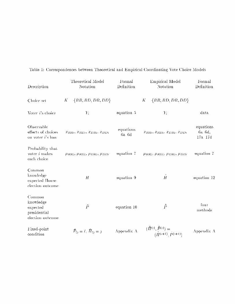
Table 1: Correspondences between Theoretical and Empirical Coordinating Vote Choice Models

Theoretical Model Formal Empirical Model FormalDescription Notation De�nition Notation De�nition

Choice set K = fRR;RD;DR;DDg | K = fRR;RD;DR;DDg |

Voter i's choice Yi equation 5 Yi data

Observablee�ects of choiceson voter i's loss

xRRi, xRDi, xDRi, xDDiequations6a{6d

xRRi, xRDi, xDRi, xDDi

equations6a{6d,17a{17d

Probability thatvoter i makeseach choice

�RRi, �RDi, �DRi, �DDi equation 7 �RRi, �RDi, �DRi, �DDi equation 7

Commonknowledgeexpected Houseelection outcome

�H equation 9 �H equation 12

Commonknowledgeexpectedpresidentialelection outcome

�P equation 10 �Pfour

methods

Fixed-pointcondition

�P`| = `, �H`| = | Appendix A( �H({); �P ({)) =

( �H({+1); �P ({+1))Appendix A

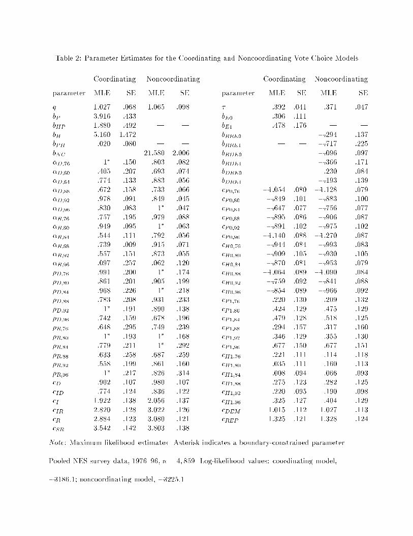
Table 2: Parameter Estimates for the Coordinating and Noncoordinating Vote Choice Models

Coordinating Noncoordinating Coordinating Noncoordinating

parameter MLE SE MLE SE parameter MLE SE MLE SE

q 1:027 :068 1:065 :098 � :392 :041 :371 :047bP 3:916 :433 | | bE0 :306 :111 | |bHP 1:880 :492 | | bE1 :478 :176 | |bH 5:160 1:472 | | bRRE0 | | �:294 :137bPH :020 :080 | | bRRE1 | | �:717 :225bNC | | 21:580 2:006 bRDE0 | | �:096 :097�D;76 1� :150 :803 :082 bRDE1 | | �:366 :171�D;80 :405 :207 :693 :074 bDRE0 | | :230 :084�D;84 :774 :133 :883 :056 bDRE1 | | �:193 :139�D;88 :672 :158 :733 :066 cP0;76 �1:054 :080 �1:128 :079�D;92 :978 :091 :849 :045 cP0;80 �:849 :101 �:883 :100�D;96 :830 :083 1� :047 cP0;84 �:647 :077 �:756 :077�R;76 :757 :195 :979 :088 cP0;88 �:895 :086 �:906 :087�R;80 :949 :095 1� :063 cP0;92 �:891 :102 �:975 :102�R;84 :544 :111 :792 :056 cP0;96 �1:140 :088 �1:270 :087�R;88 :739 :009 :915 :071 cH0;76 �:944 :084 �:993 :083�R;92 :557 :151 :873 :055 cH0;80 �:909 :105 �:930 :105�R;96 :097 :257 :062 :120 cH0;84 �:870 :081 �:953 :079�D;76 :991 :200 1� :174 cH0;88 �1:064 :089 �1:090 :084�D;80 :861 :201 :905 :199 cH0;92 �:759 :092 �:841 :088�D;84 :968 :226 1� :218 cH0;96 �:854 :089 �:966 :092�D;88 :783 :208 :931 :233 cP1;76 :220 :130 :209 :132�D;92 1� :191 :890 :138 cP1;80 :424 :129 :475 :129�D;96 :742 :159 :678 :196 cP1;84 :479 :128 :518 :125�R;76 :648 :295 :749 :239 cP1;88 :294 :157 :317 :160�R;80 1� :193 1� :168 cP1;92 :346 :129 :355 :130�R;84 :779 :211 1� :292 cP1;96 :677 :150 :677 :151�R;88 :633 :258 :687 :259 cH1;76 :221 :111 :114 :118�R;92 :558 :199 :861 :160 cH1;80 :035 :111 :160 :113�R;96 1� :217 :826 :314 cH1;84 :008 :094 :066 :093cD :902 :107 :980 :107 cH1;88 :275 :123 :282 :125cID :774 :124 :836 :122 cH1;92 :220 :095 :190 :098cI 1:922 :138 2:056 :137 cH1;96 :325 :127 :404 :129cIR 2:820 :128 3:022 :126 cDEM 1:015 :112 1:027 :113cR 2:884 :123 3:080 :121 cREP 1:325 :121 1:328 :124cSR 3:542 :142 3:803 :138

Note: Maximum likelihood estimates. Asterisk indicates a boundary-constrained parameter.

Pooled NES survey data, 1976{96, n = 4; 859. Log-likelihood values: coordinating model,

�3186:1; noncoordinating model, �3225:1.

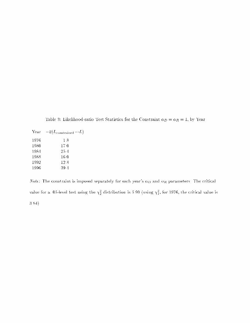
Table 3: Likelihood-ratio Test Statistics for the Constraint �D = �R = 1, by Year

Year �2(Lconstrained� L)

1976 1.81980 17.01984 25.41988 16.01992 12.81996 39.4

Note: The constraint is imposed separately for each year's �D and �R parameters. The critical

value for a .05-level test using the �22 distribution is 5.99 (using �21, for 1976, the critical value is

3.84).

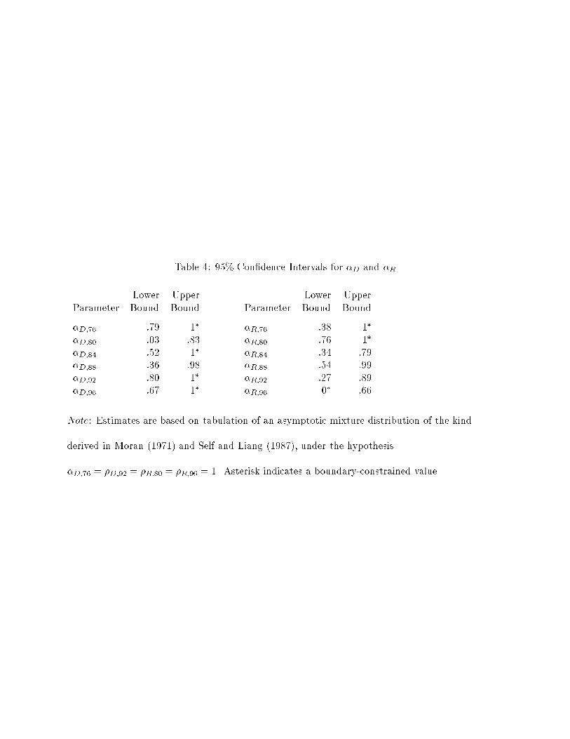
Table 4: 95% Con�dence Intervals for �D and �R

Lower Upper Lower UpperParameter Bound Bound Parameter Bound Bound

�D;76 :79 1� �R;76 :38 1�

�D;80 :03 :83 �R;80 :76 1�

�D;84 :52 1� �R;84 :34 :79�D;88 :36 :98 �R;88 :54 :99�D;92 :80 1� �R;92 :27 :89�D;96 :67 1� �R;96 0� :66

Note: Estimates are based on tabulation of an asymptotic mixture distribution of the kind

derived in Moran (1971) and Self and Liang (1987), under the hypothesis

�D;76 = �D;92 = �R;80 = �R;96 = 1. Asterisk indicates a boundary-constrained value.

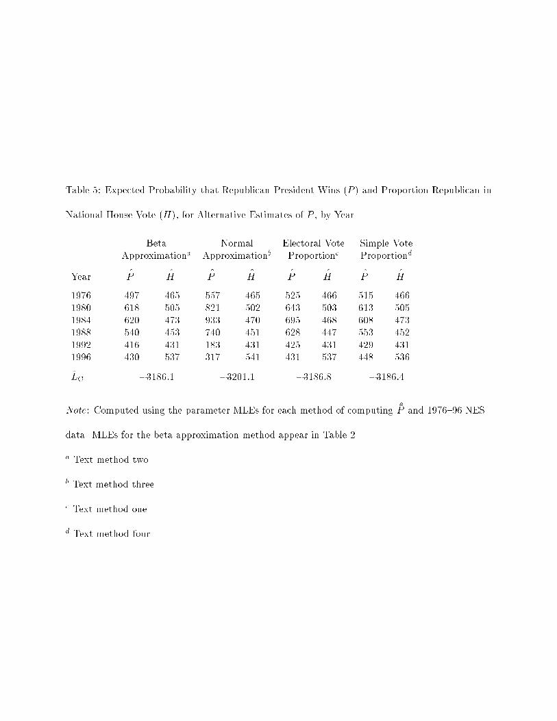
Table 5: Expected Probability that Republican President Wins ( �P ) and Proportion Republican in

National House Vote ( �H), for Alternative Estimates of �P , by Year

Beta Normal Electoral Vote Simple VoteApproximationa Approximationb Proportionc Proportiond

Year �P �H �P �H �P �H �P �H

1976 .497 .465 .557 .465 .525 .466 .515 .4661980 .618 .505 .821 .502 .643 .503 .613 .5051984 .620 .473 .933 .470 .695 .468 .608 .4731988 .540 .453 .740 .451 .628 .447 .553 .4521992 .416 .431 .183 .431 .425 .431 .429 .4311996 .430 .537 .317 .541 .431 .537 .448 .536

LC �3186:1 �3201:1 �3186:8 �3186:4

Note: Computed using the parameter MLEs for each method of computing �P and 1976{96 NES

data. MLEs for the beta approximation method appear in Table 2.

a Text method two.

b Text method three.

c Text method one.

d Text method four.

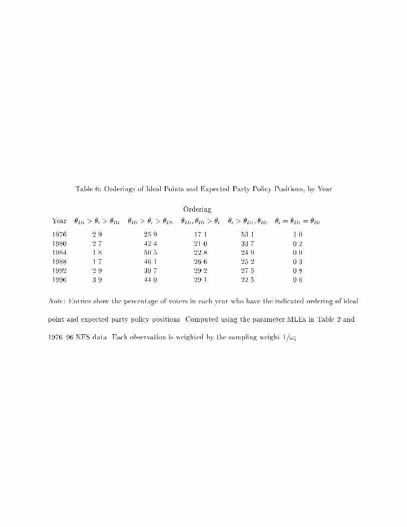
Table 6: Orderings of Ideal Points and Expected Party Policy Positions, by Year

Ordering

Year �Di > �i > �Ri �Ri > �i > �Di �Di; �Ri > �i �i > �Di; �Ri �i = �Di = �Ri

1976 2.9 25.9 17.1 53.1 1.01980 2.7 42.4 21.0 33.7 0.21984 1.8 50.5 22.8 24.9 0.01988 1.7 46.1 26.6 25.2 0.31992 2.9 39.7 29.2 27.5 0.81996 3.9 44.0 29.1 22.5 0.6

Note: Entries show the percentage of voters in each year who have the indicated ordering of ideal

point and expected party policy positions. Computed using the parameter MLEs in Table 2 and

1976{96 NES data. Each observation is weighted by the sampling weight 1=!i.

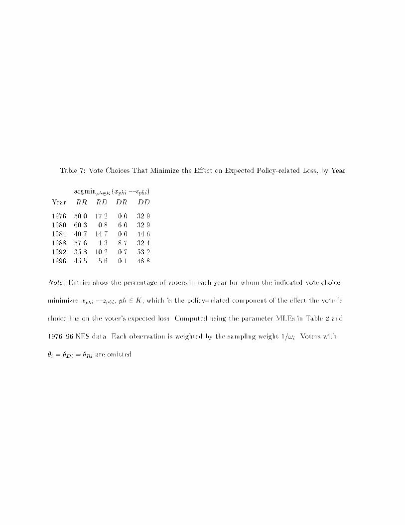
Table 7: Vote Choices That Minimize the E�ect on Expected Policy-related Loss, by Year

argminph2K(xphi � zphi)

Year RR RD DR DD

1976 50.0 17.2 0.0 32.91980 60.3 0.8 6.0 32.91984 40.7 14.7 0.0 44.61988 57.6 1.3 8.7 32.41992 35.8 10.2 0.7 53.21996 45.5 5.6 0.1 48.8

Note: Entries show the percentage of voters in each year for whom the indicated vote choice

minimizes xphi � zphi, ph 2 K, which is the policy-related component of the e�ect the voter's

choice has on the voter's expected loss. Computed using the parameter MLEs in Table 2 and

1976{96 NES data. Each observation is weighted by the sampling weight 1=!i. Voters with

�i = �Di = �Ri are omitted.