(VVHQWLDO 6SUHDGVKHHWV %RRN - University of … Excel E} For multiple rows/columns, select the number you wish to insert/delete and proceed as above. $GMXVWLQJURZVKHLJKWDQ GFROXPQZLGWK

Information Services

ITwww.york.ac.uk/it-services/training

EssentialSpreadsheets

Book 1

Essential SpreadsheetsBook 1

This material explains how to use spreadsheets, and is based around:

Microsoft Excel 2016 on a University of York Managed PC Google Sheets running in an up-to-date browser

Screen-shots have been chosen to reflect the similarities and differences

between these.

Every attempt has been made to ensure the accuracy of the information

provided, however you may find some differences when working with other

or personalised systems.

Note This information is correct at the time of writing, but new

features are added to Google Sheets on a regular basis – check

periodically for new options appearing in menus.

A collection of exercises is also available, with task documents in both Excel

and Google Sheets format.

See also our support site: https://goo.gl/OY1Wzy

Last Updated: August 2017

~Contents~

Part 1~ Spreadsheet Basics 11 ~ Introducing spreadsheets 1

1.1 - Choosing the correct tool 11.2 - Creating and Saving 11.3 - Spreadsheet workspace 21.4 - Managing the workspace 3

2 ~ Entering and editing data 62.1 - Data entry 62.2 - Selecting cells 72.3 - Saving time when entering data 8

3 ~ Presenting a spreadsheet 103.1 - Number and date/time format tools 103.2 - Percentages 113.3 - Dates and Times 123.4 - Currency 133.5 - Text 14

4 ~ Performing calculations 154.1 - Basic arithmetic 154.2 - Using functions 164.3 - Replicating formulae 184.4 - Absolute cell addressing 184.5 - References between worksheets 19

Part 2~ Further functions 205 ~ Named ranges 20

5.1 - Creating named ranges 205.2 - Using named ranges 21

6 ~ Finding and inserting functions 236.1 - Excel – Function Library 236.2 - Google Sheets 24

7 ~ Conditional functions 257.1 - IF() 257.2 - Conditional COUNT, SUM and AVERAGE 277.3 - Multiple criteria with COUNT, SUM and IF 29

8 ~ Time and date calculations 308.1 - Dates 308.2 - Times and Duration 308.3 - Date and Time functions 318.4 - Date & Time custom formatting 32

9 ~ Other useful functions 33

Part 1~Spreadsheet Basics

1


1 ~ Introducing spreadsheetsSpreadsheets were developed to store, analyse and manipulate data. They are now commonly used for working with sets of data containing both text and numbers.

Every spreadsheet consists of a large grid of cells to store data which can then be manipulated using formulae

Each cell has an address which consists of the column letter and row number

Many spreadsheet documents contain several individual sheets that can reference values in other sheets in the file

Spreadsheets can also produce graphs and other data visualisations

1.1 - Choosing the correct toolThe University provides support for two spreadsheet tools:

Microsoft Excel, part of Microsoft Office.

Google Sheets, one of Google’s cloud applications.

The two applications share many common features, and similar functionality, however Google sheets are particularly useful when working collaboratively.

When necessary, data can easily be moved between them.

This guide coves both tools, highlighting the differences and similarities so that users are able to pick the best tool for the task at hand.

1.2 - Creating and SavingNew Excel spreadsheets are created from the File tab of the application, and must be saved using File > Save As…, at which point the location of the file is also chosen. You must also remember to save changes to the spreadsheet.

When creating a new Google spreadsheet, it is recommended that in Driveyou first locate the folder in which it is to reside before choosing New > Google Sheets. Google sheets are saved repeatedly and automatically without any action by the user.

2

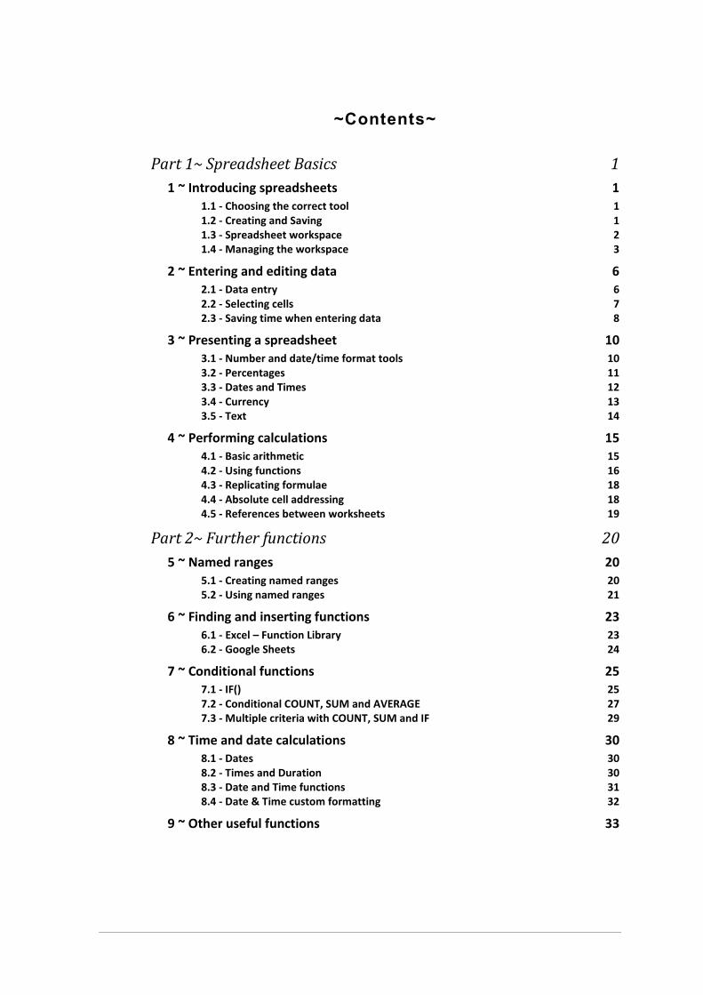
1.3 - Spreadsheet workspace

Excel 2016 (PC Version)

Active cell Anything you type will be entered in the active cell. Any formatting you apply will affect only the active cell.

Row number Rows are numbered consecutively from 1

Column letter Columns are labelled consecutively with letters. On reaching ‘Z’, columns are labelled AA, AB, AC and so on.

Formula bar This shows the content of the active cell, and can be used to edit it.

Worksheet tabs

Each workbook may consist of several worksheets, and the tabs are used to switch between them.

Right-click or double-click the tab to rename or add colour markers

Zoom controls Spreadsheets can be very large, so the Zoom controls allow you to view a larger/smaller area of worksheet

Ribbon The ribbon includes the tabs and controls for all the essential features of the Excel spreadsheet

Formula bar

Active cellColumn letter

Row number

Worksheet tabs

New worksheet

Zoom controls

Ribbon


3

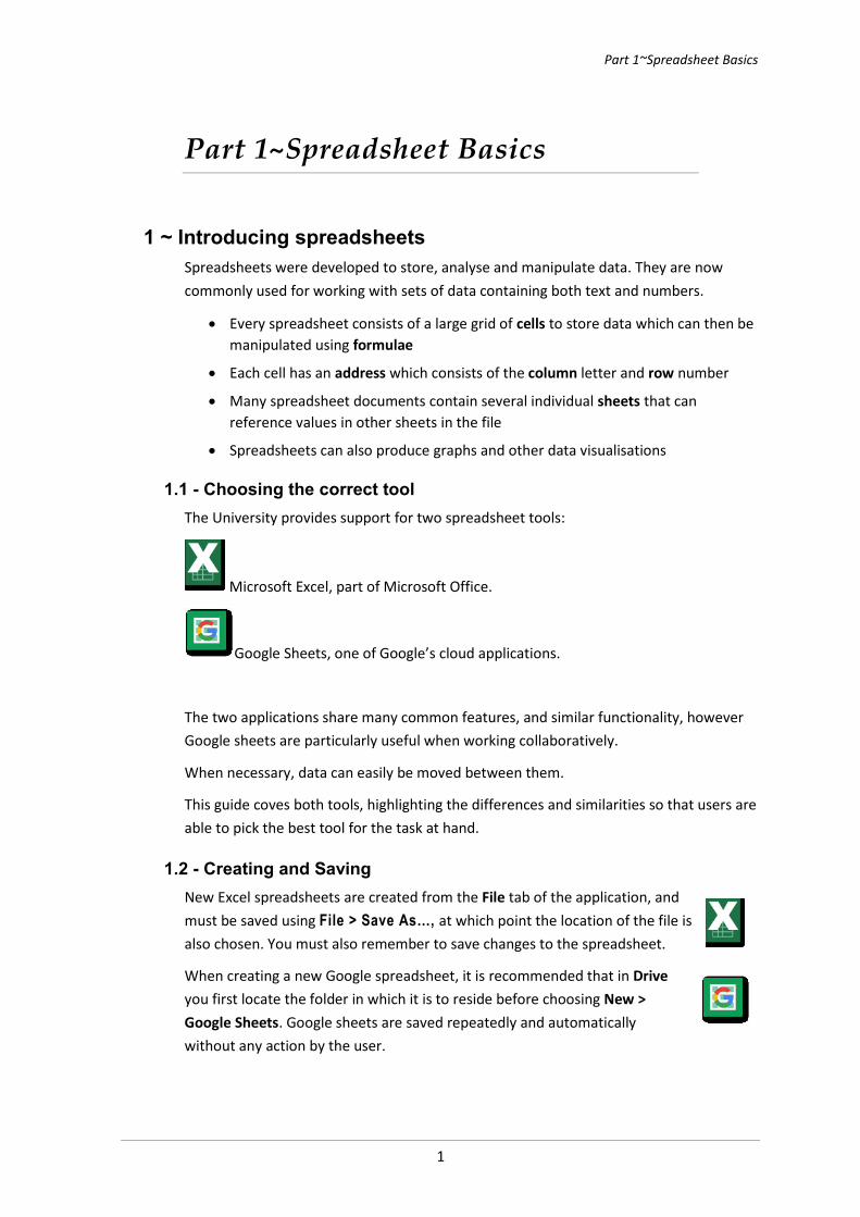
Google Sheets

1.4 - Managing the workspaceA new spreadsheet (or new worksheet) will contain a large number of cells of a standard width and height. You will often need to make adjustments to these:

Add, remove or rename worksheets

Change the height of one or more rows

Change the width of one or more columns

Insert extra rows or columns

Remove one or more rows or columns

Note Although you can remove individual cells (or groups of cells), it is better always to remove entire rows/columns – otherwise a ‘hole’ is created that has to be filled by shifting other cells

Bear in mind that removing (deleting) a cell is not the same thing as clearing the contents of a cell.

Formula bar

Active cellColumn letter

Row number

Worksheet tabs

Sheet options

All sheets

New worksheet

File share settings

4

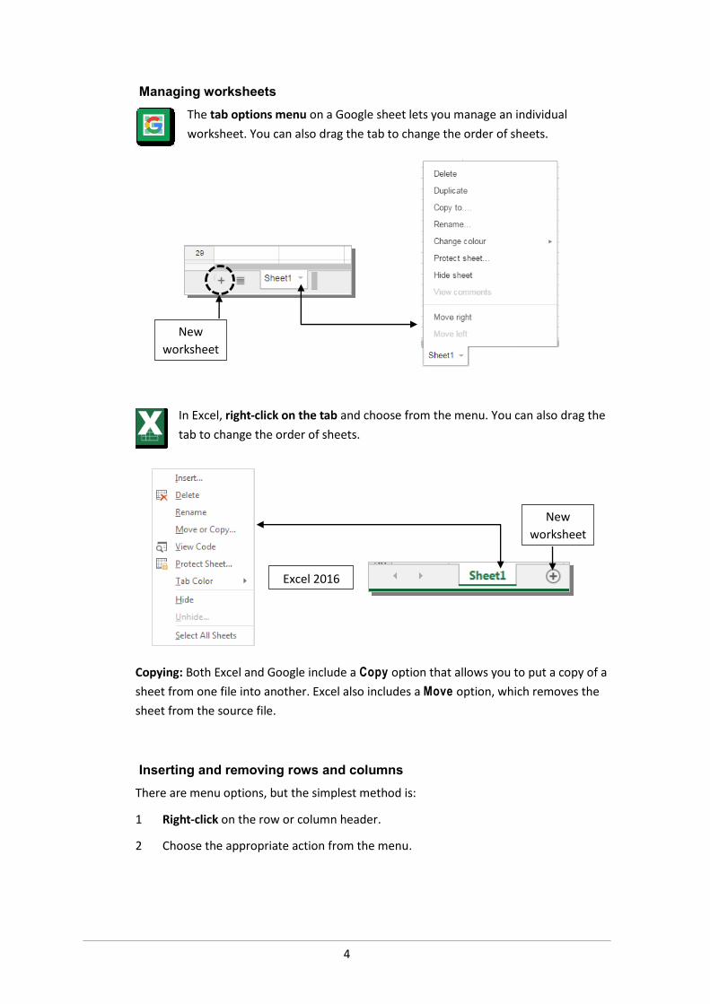
Managing worksheetsThe tab options menu on a Google sheet lets you manage an individual worksheet. You can also drag the tab to change the order of sheets.

In Excel, right-click on the tab and choose from the menu. You can also drag the tab to change the order of sheets.

Copying: Both Excel and Google include a Copy option that allows you to put a copy of a sheet from one file into another. Excel also includes a Move option, which removes the sheet from the source file.

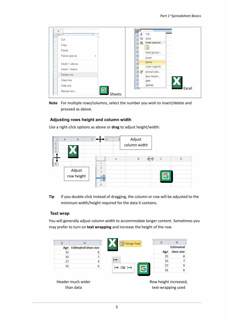
Inserting and removing rows and columnsThere are menu options, but the simplest method is:

1 Right-click on the row or column header.

2 Choose the appropriate action from the menu.

New worksheet

New worksheet

Excel 2016


5

SheetsExcel

Note For multiple rows/columns, select the number you wish to insert/delete and proceed as above.

Adjusting rows height and column widthUse a right-click options as above or drag to adjust height/width:

Tip If you double-click instead of dragging, the column or row will be adjusted to the minimum width/height required for the data it contains.

Text wrapYou will generally adjust column width to accommodate longer content. Sometimes you may prefer to turn on text wrapping and increase the height of the row.

Adjust column width

Adjust row height

Header much wider than data

Row height increased, text-wrapping used

6

2 ~ Entering and editing dataA cell can contain one of three things:

text data (anything not understood to be a number or formula) numerical data (including Dates, times, percentages and currency) a formula

Cells containing formulae normally display the result of the calculation.

Text data Left-aligned by defaultFormula bar displays actual contentContent preceded by a single quote is always regarded as text

Numeric data Right-aligned by defaultRounding will be applied automaticallyLeading zeros removed

Formula Aligned according to type of result (text or numeric)Cell displays result of formulaFormula bar shows formula

Both Excel and Google spreadsheets follow these conventions.

2.1 - Data entryWhen constructing or editing a spreadsheet you will need to be able to navigate between cells and enter content. It’s mostly intuitive, but there are some useful points to be aware of:

Click or use the navigation (arrow) keys to move to a specific cell

Typing in a cell overwrites existing content if it is not blank

To edit a cell that already contains data, double-click or select it and edit the content in the formula bar

Once data has been entered or edited, you must press Enter or Tab. At this point the spreadsheet will:

o Check your data makes sense (and report errors)o Decide how numerical values should be formattedo Update all calculated values

Resist the urge to click in another cell or use the cursor keys as they have a different effect when editing cell content.

Pressing Escape (Esc) key at any point during data entry will abort the process

Pressing Delete (Del) key will clear the contents, leaving the format unchanged

Note Pressing Enter after data entry moves to the next cell down.

Pressing Tab will move to the right. Holding Shift when pressing either Enter or Tab will move the cursor in the opposite direction.


7

Excel: the accept/reject edit controls can also be used to accept/reject an edit.

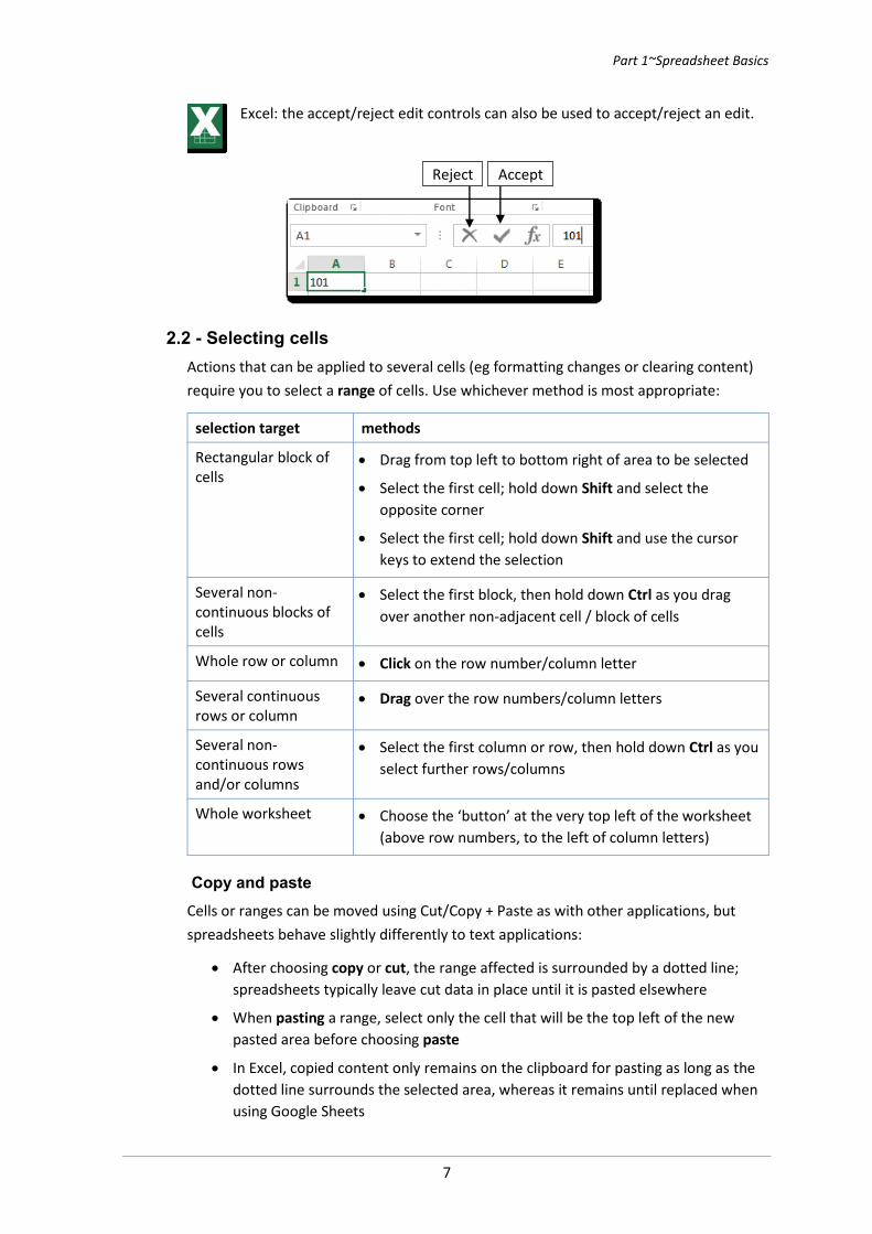
2.2 - Selecting cellsActions that can be applied to several cells (eg formatting changes or clearing content) require you to select a range of cells. Use whichever method is most appropriate:

selection target methods

Rectangular block of cells

Drag from top left to bottom right of area to be selected

Select the first cell; hold down Shift and select the opposite corner

Select the first cell; hold down Shift and use the cursor keys to extend the selection

Several non-continuous blocks of cells

Select the first block, then hold down Ctrl as you drag over another non-adjacent cell / block of cells

Whole row or column Click on the row number/column letter

Several continuous rows or column

Drag over the row numbers/column letters

Several non-continuous rows and/or columns

Select the first column or row, then hold down Ctrl as you select further rows/columns

Whole worksheet Choose the ‘button’ at the very top left of the worksheet (above row numbers, to the left of column letters)

Copy and pasteCells or ranges can be moved using Cut/Copy + Paste as with other applications, but spreadsheets behave slightly differently to text applications:

After choosing copy or cut, the range affected is surrounded by a dotted line; spreadsheets typically leave cut data in place until it is pasted elsewhere

When pasting a range, select only the cell that will be the top left of the new pasted area before choosing paste

In Excel, copied content only remains on the clipboard for pasting as long as the dotted line surrounds the selected area, whereas it remains until replaced when using Google Sheets

AcceptReject

8

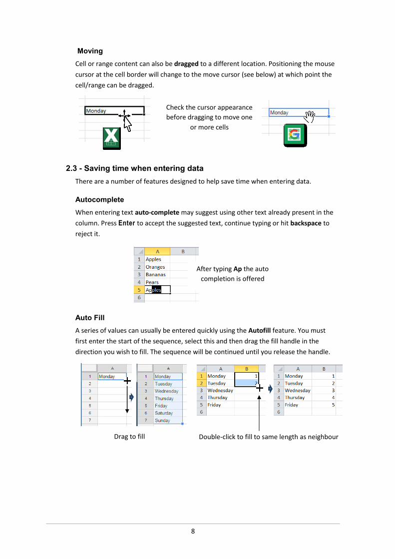
MovingCell or range content can also be dragged to a different location. Positioning the mouse cursor at the cell border will change to the move cursor (see below) at which point the cell/range can be dragged.

2.3 - Saving time when entering dataThere are a number of features designed to help save time when entering data.

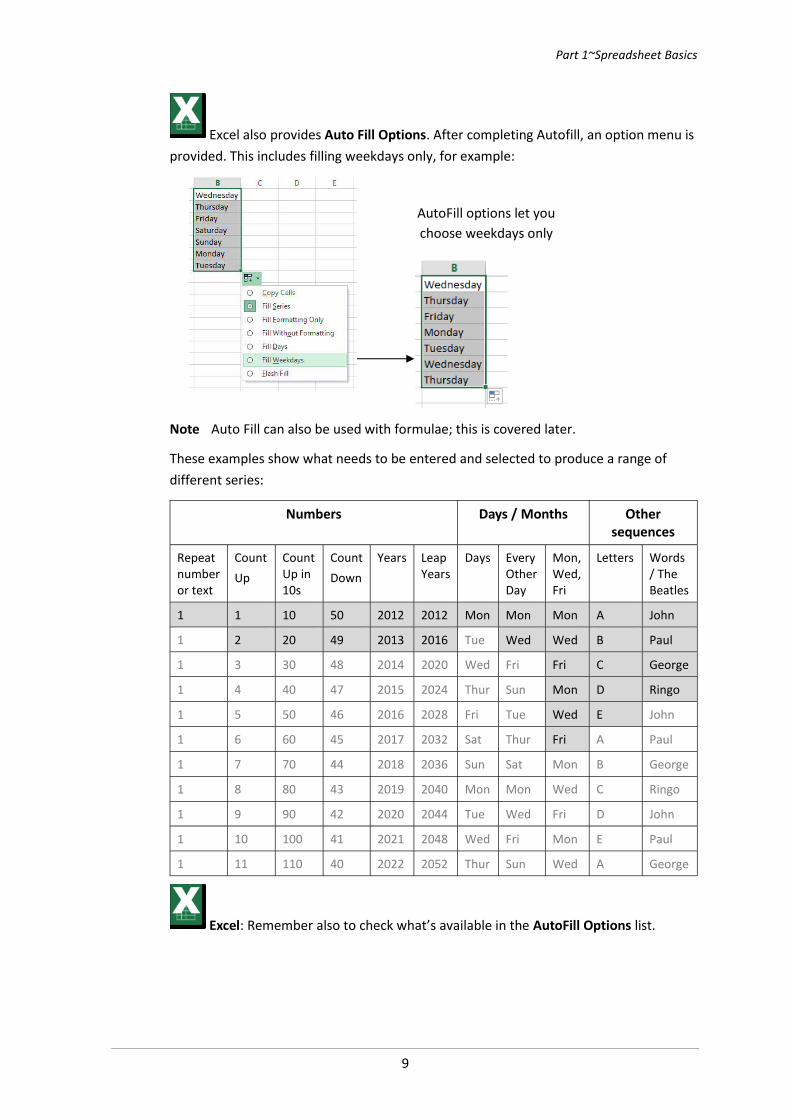
AutocompleteWhen entering text auto-complete may suggest using other text already present in the column. Press Enter to accept the suggested text, continue typing or hit backspace to reject it.

Auto FillA series of values can usually be entered quickly using the Autofill feature. You must first enter the start of the sequence, select this and then drag the fill handle in the direction you wish to fill. The sequence will be continued until you release the handle.

Check the cursor appearance before dragging to move one

or more cells

After typing Ap the auto completion is offered

Drag to fill Double-click to fill to same length as neighbour


9

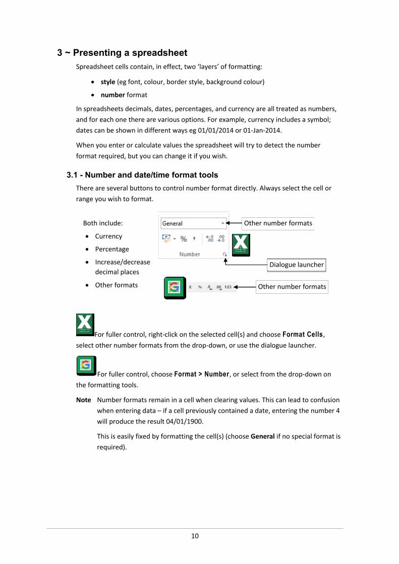
Excel also provides Auto Fill Options. After completing Autofill, an option menu is provided. This includes filling weekdays only, for example:

Note Auto Fill can also be used with formulae; this is covered later.

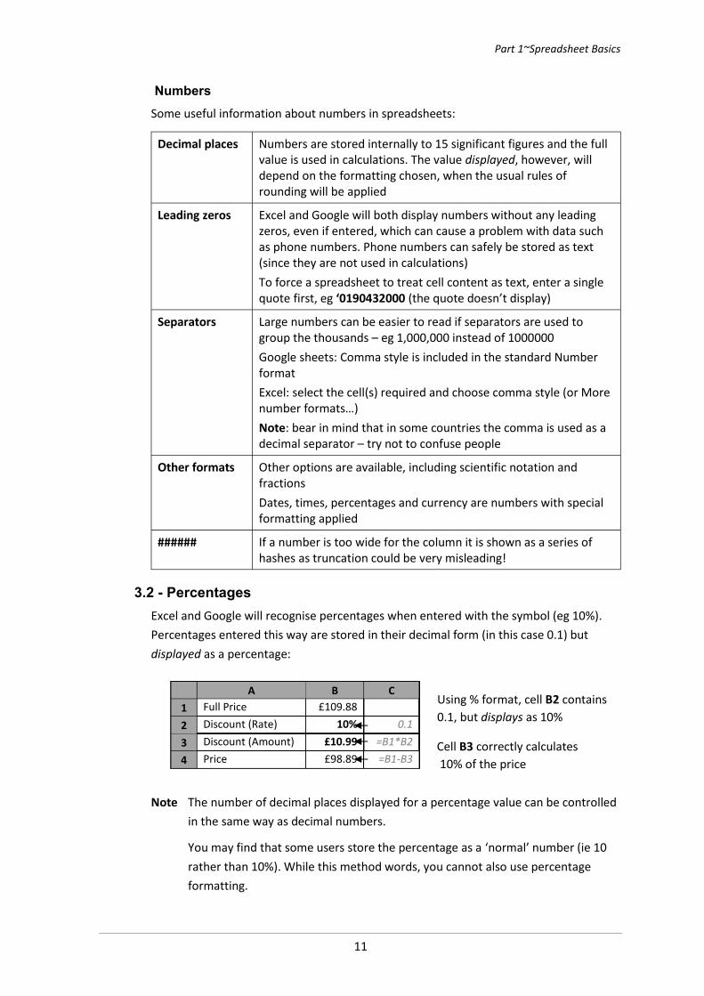
These examples show what needs to be entered and selected to produce a range of different series:

Numbers Days / Months Other sequences

Repeat number or text

CountUp

Count Up in 10s

CountDown

Years Leap Years

Days Every Other Day

Mon, Wed, Fri

Letters Words / The Beatles

1 1 10 50 2012 2012 Mon Mon Mon A John

1 2 20 49 2013 2016 Tue Wed Wed B Paul

1 3 30 48 2014 2020 Wed Fri Fri C George

1 4 40 47 2015 2024 Thur Sun Mon D Ringo

1 5 50 46 2016 2028 Fri Tue Wed E John

1 6 60 45 2017 2032 Sat Thur Fri A Paul

1 7 70 44 2018 2036 Sun Sat Mon B George

1 8 80 43 2019 2040 Mon Mon Wed C Ringo

1 9 90 42 2020 2044 Tue Wed Fri D John

1 10 100 41 2021 2048 Wed Fri Mon E Paul

1 11 110 40 2022 2052 Thur Sun Wed A George

Excel: Remember also to check what’s available in the AutoFill Options list.

AutoFill options let you choose weekdays only

10

3 ~ Presenting a spreadsheetSpreadsheet cells contain, in effect, two ‘layers’ of formatting:

style (eg font, colour, border style, background colour)

number format

In spreadsheets decimals, dates, percentages, and currency are all treated as numbers, and for each one there are various options. For example, currency includes a symbol; dates can be shown in different ways eg 01/01/2014 or 01-Jan-2014.

When you enter or calculate values the spreadsheet will try to detect the number format required, but you can change it if you wish.

3.1 - Number and date/time format toolsThere are several buttons to control number format directly. Always select the cell or range you wish to format.

For fuller control, right-click on the selected cell(s) and choose Format Cells,select other number formats from the drop-down, or use the dialogue launcher.

For fuller control, choose Format > Number, or select from the drop-down on the formatting tools.

Note Number formats remain in a cell when clearing values. This can lead to confusion when entering data – if a cell previously contained a date, entering the number 4 will produce the result 04/01/1900.

This is easily fixed by formatting the cell(s) (choose General if no special format is required).

Both include:

Currency

Percentage

Increase/decrease decimal places

Other formats

Other number formats

Other number formats

Dialogue launcher


11

NumbersSome useful information about numbers in spreadsheets:

Decimal places Numbers are stored internally to 15 significant figures and the full value is used in calculations. The value displayed, however, will depend on the formatting chosen, when the usual rules of rounding will be applied

Leading zeros Excel and Google will both display numbers without any leading zeros, even if entered, which can cause a problem with data such as phone numbers. Phone numbers can safely be stored as text (since they are not used in calculations)To force a spreadsheet to treat cell content as text, enter a single quote first, eg ‘0190432000 (the quote doesn’t display)

Separators Large numbers can be easier to read if separators are used to group the thousands – eg 1,000,000 instead of 1000000Google sheets: Comma style is included in the standard Number formatExcel: select the cell(s) required and choose comma style (or More number formats…)Note: bear in mind that in some countries the comma is used as a decimal separator – try not to confuse people

Other formats Other options are available, including scientific notation and fractionsDates, times, percentages and currency are numbers with special formatting applied

###### If a number is too wide for the column it is shown as a series of hashes as truncation could be very misleading!

3.2 - PercentagesExcel and Google will recognise percentages when entered with the symbol (eg 10%). Percentages entered this way are stored in their decimal form (in this case 0.1) but displayed as a percentage:

Note The number of decimal places displayed for a percentage value can be controlled in the same way as decimal numbers.

You may find that some users store the percentage as a ‘normal’ number (ie 10 rather than 10%). While this method words, you cannot also use percentage formatting.

A B C1 Full Price £109.882 Discount (Rate) 10% 0.13 Discount (Amount) £10.99 =B1*B24 Price £98.89 =B1-B3

Using % format, cell B2 contains 0.1, but displays as 10%

Cell B3 correctly calculates10% of the price

12

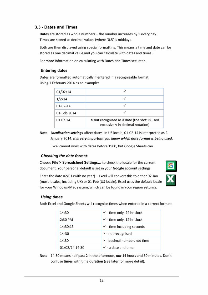
3.3 - Dates and TimesDates are stored as whole numbers – the number increases by 1 every day.Times are stored as decimal values (where ‘0.5’ is midday).

Both are then displayed using special formatting. This means a time and date can be stored as one decimal value and you can calculate with dates and times.

For more information on calculating with Dates and Times see later.

Entering datesDates are formatted automatically if entered in a recognisable format. Using 1 February 2014 as an example:

01/02/14

1/2/14

01-02-14

01-Feb-2014

01.02.14 not recognised as a date (the ‘dot’ is usedexclusively in decimal notation)

Note Localisation settings affect dates. In US locale, 01-02-14 is interpreted as 2 January 2014. It is very important you know which date format is being used.

Excel cannot work with dates before 1900, but Google Sheets can.

Checking the date format:Choose File > Spreadsheet Settings… to check the locale for the current document. Your personal default is set in your Google account settings.

Enter the date 02/01 (with no year) – Excel will convert this to either 02-Jan (most locales, including UK) or 01-Feb (US locale). Excel uses the default locale for your Windows/Mac system, which can be found in your region settings.

Using timesBoth Excel and Google Sheets will recognise times when entered in a correct format:

14:30 - time only, 24 hr clock

2:30 PM - time only, 12 hr clock

14:30:15 - time including seconds

14-30 - not recognised

14.30 - decimal number, not time

01/02/14 14:30 - a date and time

Note 14:30 means half past 2 in the afternoon, not 14 hours and 30 minutes. Don’t confuse times with time duration (see later for more detail).


13

3.4 - CurrencyCurrency can be entered in two different ways:

Enter the sum, including the currency symbol, eg: £1.50. This will be recognised as currency and formatted appropriately

Enter the value only and then select the currency format

Note Spreadsheets do not automatically convert currency values using number formatting - £1.50 + €1.50 will give a result of 3.00.

Excel and Google Sheets include two currency-formatting styles: Currency and one referred to as Accounting or Financial, which both display negative values in brackets and have other subtle differences with Currency.

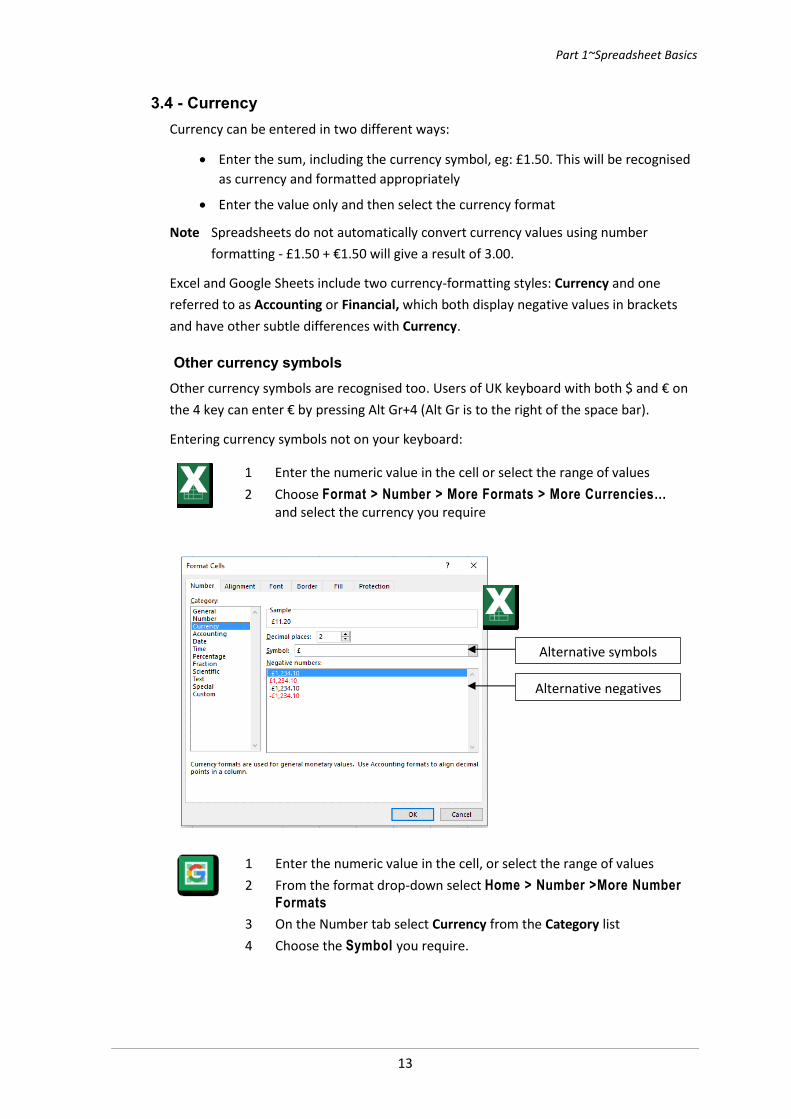
Other currency symbolsOther currency symbols are recognised too. Users of UK keyboard with both $ and € on the 4 key can enter € by pressing Alt Gr+4 (Alt Gr is to the right of the space bar).

Entering currency symbols not on your keyboard:

1 Enter the numeric value in the cell or select the range of values2 Choose Format > Number > More Formats > More Currencies…

and select the currency you require

1 Enter the numeric value in the cell, or select the range of values2 From the format drop-down select Home > Number >More Number

Formats3 On the Number tab select Currency from the Category list4 Choose the Symbol you require.

Alternative symbols

Alternative negatives

14

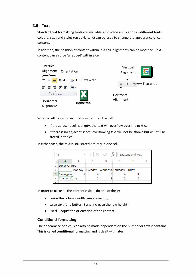
3.5 - TextStandard text formatting tools are available as in office applications – different fonts, colours, sizes and styles (eg bold, italic) can be used to change the appearance of cell content.

In addition, the position of content within in a cell (alignment) can be modified. Text content can also be ‘wrapped’ within a cell:

When a cell contains text that is wider than the cell:

if the adjacent cell is empty, the text will overflow over the next cell

if there is no adjacent space, overflowing text will not be shown but will still be stored in the cell

In either case, the text is still stored entirely in one cell.

In order to make all the content visible, do one of these:

resize the column width (see above, p5)

wrap text for a better fit and increase the row height

Excel – adjust the orientation of the content

Conditional formattingThe appearance of a cell can also be made dependent on the number or text it contains. This is called conditional formatting and is dealt with later.

Vertical Alignment

HorizontalAlignmentHorizontal

Alignment

Vertical Alignment

Text wrapText wrap

Orientation

Home tab


15

4 ~ Performing calculationsFormulae are entered directly into the cell where you want the answer to appear, and always start with an equals sign (=). Some important points about using formulae:

Rather than enter numerical values in a formula, you should reference values held in spreadsheet cells wherever possible

Never enter the ‘answer’ value directly in a cell, no-matter how easy the calculation is – use a formula if it can be calculated from other cell values so it will update if input values change

As with data entry, always press Enter after entering a formula

4.1 - Basic arithmeticFormulae can contain basic arithmetic. Use the following symbols for basic arithmetic:

+ Add * Multiply

- Subtract / Divide

^ To the power of

Here is a formula that subtracts two cell values. The result is shown in cell A3, but you will also see the formula in the formula bar, = A1 – A2

fx = A1 – A2A B C

1 92 63 34

Entering cell references: When entering a formula, a cell reference can be typed directly, entered by clicking on it, or by selecting with the cursor keys.

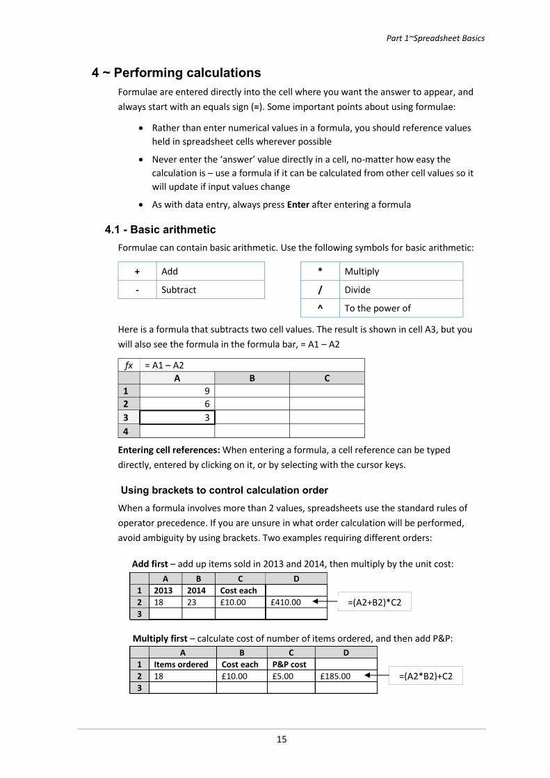
Using brackets to control calculation order When a formula involves more than 2 values, spreadsheets use the standard rules of operator precedence. If you are unsure in what order calculation will be performed, avoid ambiguity by using brackets. Two examples requiring different orders:

A B C D1 2013 2014 Cost each2 18 23 £10.00 £410.003

=(A2+B2)*C2

A B C D1 Items ordered Cost each P&P cost2 18 £10.00 £5.00 £185.003

=(A2*B2)+C2

Add first – add up items sold in 2013 and 2014, then multiply by the unit cost:

Multiply first – calculate cost of number of items ordered, and then add P&P:

16

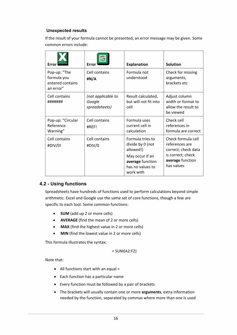
Unexpected resultsIf the result of your formula cannot be presented, an error message may be given. Some common errors include:

Error Error Explanation Solution

Pop-up: “The formula you entered contains an error”

Cell contains#N/A

Formula not understood

Check for missing arguments, brackets etc

Cell contains #######

(not applicable to Google spreadsheets)

Result calculated, but will not fit into cell

Adjust column width or format to allow the result to be viewed

Pop-up: “Circular Reference Warning”

Cell contains#REF!

Formula uses current cell in calculation

Check cell references in formula are correct

Cell contains#DIV/0!

Cell contains#DIV/0

Formula tries to divide by 0 (not allowed!)May occur if an average function has no values to work with

Check formula cell references are correct; check data is correct; check average function has values

4.2 - Using functionsSpreadsheets have hundreds of functions used to perform calculations beyond simple arithmetic. Excel and Google use the same set of core functions, though a few are specific to each tool. Some common functions:

SUM (add up 2 or more cells) AVERAGE (find the mean of 2 or more cells) MAX (find the highest value in 2 or more cells) MIN (find the lowest value in 2 or more cells)

This formula illustrates the syntax:

= SUM(A2:F2)

Note that:

All functions start with an equal =

Each function has a particular name

Every function must be followed by a pair of brackets

The brackets will usually contain one or more arguments, extra information needed by the function, separated by commas where more than one is used


17

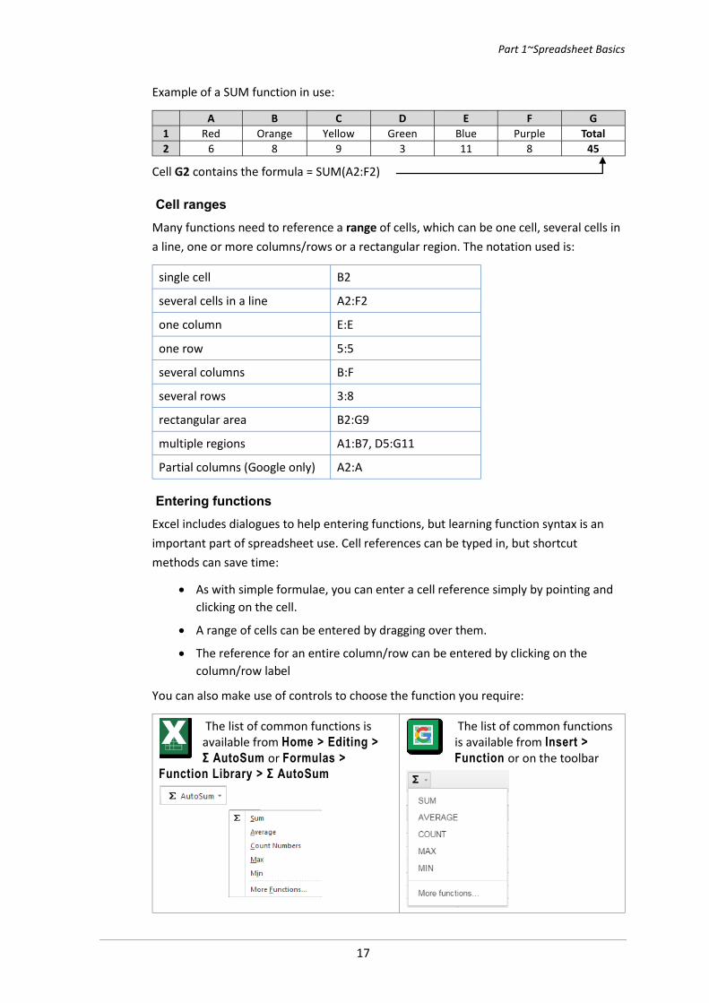
Example of a SUM function in use:

A B C D E F G1 Red Orange Yellow Green Blue Purple Total2 6 8 9 3 11 8 45

Cell G2 contains the formula = SUM(A2:F2)

Cell rangesMany functions need to reference a range of cells, which can be one cell, several cells in a line, one or more columns/rows or a rectangular region. The notation used is:

single cell B2

several cells in a line A2:F2

one column E:E

one row 5:5

several columns B:F

several rows 3:8

rectangular area B2:G9

multiple regions A1:B7, D5:G11

Partial columns (Google only) A2:A

Entering functionsExcel includes dialogues to help entering functions, but learning function syntax is an important part of spreadsheet use. Cell references can be typed in, but shortcut methods can save time:

As with simple formulae, you can enter a cell reference simply by pointing and clicking on the cell.

A range of cells can be entered by dragging over them.

The reference for an entire column/row can be entered by clicking on the column/row label

You can also make use of controls to choose the function you require:

The list of common functions is available from Home > Editing > Σ AutoSum or Formulas >

Function Library > Σ AutoSum

The list of common functions is available from Insert > Function or on the toolbar

18

There are several functions that count the number of values:

COUNT(range) the number of numerical values in the range

COUNTA(range) the number of all types of value in the range

COUNTBLANK(range) the number of blank cells in the range

COUNTUNIQUE(range) the number of unique values in the range(Google Sheets only)

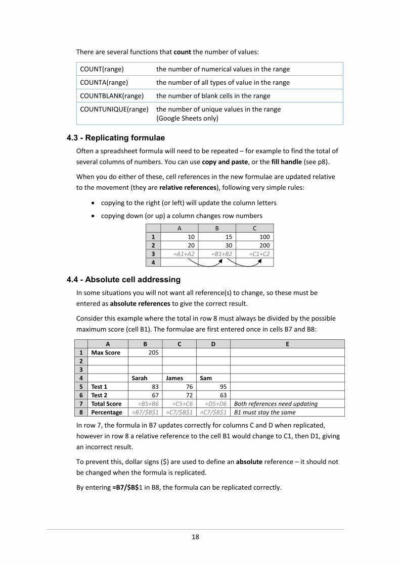
4.3 - Replicating formulaeOften a spreadsheet formula will need to be repeated – for example to find the total of several columns of numbers. You can use copy and paste, or the fill handle (see p8).

When you do either of these, cell references in the new formulae are updated relative to the movement (they are relative references), following very simple rules:

copying to the right (or left) will update the column letters

copying down (or up) a column changes row numbersA B C

1 10 15 1002 20 30 2003 =A1+A2 =B1+B2 =C1+C24

4.4 - Absolute cell addressingIn some situations you will not want all reference(s) to change, so these must be entered as absolute references to give the correct result.

Consider this example where the total in row 8 must always be divided by the possible maximum score (cell B1). The formulae are first entered once in cells B7 and B8:

A B C D E1 Max Score 205234 Sarah James Sam5 Test 1 83 76 956 Test 2 67 72 637 Total Score =B5+B6 =C5+C6 =D5+D6 Both references need updating8 Percentage =B7/$B$1 =C7/$B$1 =C7/$B$1 B1 must stay the same

In row 7, the formula in B7 updates correctly for columns C and D when replicated, however in row 8 a relative reference to the cell B1 would change to C1, then D1, giving an incorrect result.

To prevent this, dollar signs ($) are used to define an absolute reference – it should not be changed when the formula is replicated.

By entering =B7/$B$1 in B8, the formula can be replicated correctly.


19

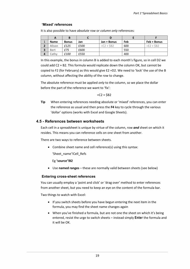
‘Mixed’ referencesIt is also possible to have absolute row or column only references:

A B C D E F1 Name Bonus Jan Jan + Bonus Feb Feb + Bonus2 Alison £125 £500 =C2 + $B2 600 =E2 + $B23 Bert £75 £600 5504 Cathy £100 £550 400

In this example, the bonus in column B is added to each month’s figure, so in cell D2 we could add C2 + B2. This formula would replicate down the column OK, but cannot be copied to F2 (for February) as this would give E2 +D2. We need to ‘lock’ the use of the B column, without affecting the ability of the row to change.

The absolute reference must be applied only to the column, so we place the dollar before the part of the reference we want to ‘fix’:

=C2 + $B2

Tip When entering references needing absolute or ‘mixed’ references, you can enter the reference as usual and then press the F4 key to cycle through the various ‘dollar’ options (works with Excel and Google Sheets).

4.5 - References between worksheetsEach cell in a spreadsheet is unique by virtue of the column, row and sheet on which it resides. This means you can reference cells on one sheet from another.

There are two ways to reference between sheets.

Combine sheet name and cell reference(s) using this syntax:

‘Sheet_name’!Cell_Refs

Eg ‘source’!B2

Use named ranges – these are normally valid between sheets (see below)

Entering cross-sheet referencesYou can usually employ a ‘point and click’ or ‘drag over’ method to enter references from another sheet, but you need to keep an eye on the content of the formula bar.

Two things to watch with Excel:

If you switch sheets before you have begun entering the next item in the formula, you may find the sheet name changes again

When you’ve finished a formula, but are not one the sheet on which it’s being entered, resist the urge to switch sheets – instead simply Enter the formula and it will be OK.

20

Part 2~Further functions

5 ~ Named rangesMost formulae need to reference cells or ranges. An alternative to the usual reference style (eg A1) is to assign names which are used in place of the cell or range address.

For example, =A1*B1 might become =Cost*Quantity. They help reduce errors by:

making spreadsheet formulae more meaningful

avoiding the need for ‘dollar’ references

You can name: a single cell, a whole column or row, or a rectangular range of cells.

As names must not be ambiguous in formulae, there are some naming rules:

They must start with a letter, but may contain numbers

They must not contain spaces – use underscore, dashes or ‘camelCase’

They must not be reserved words, or be a valid cell reference (eg AB123)

5.1 - Creating named rangesThe methods are different in Excel and Google Sheets, but you should always first select the cell or range to be named. If you are working with listed values and the number of rows in use may change, select entire columns rather than just the rows currently in use.

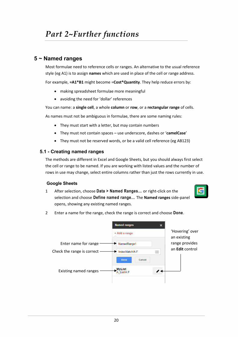
Google Sheets1 After selection, choose Data > Named Ranges… or right-click on the

selection and choose Define named range… The Named ranges side-panel opens, showing any existing named ranges.

2 Enter a name for the range, check the range is correct and choose Done.

Enter name for range

Check the range is correct

Existing named ranges

‘Hovering’ over an existing range provides an Edit control


21

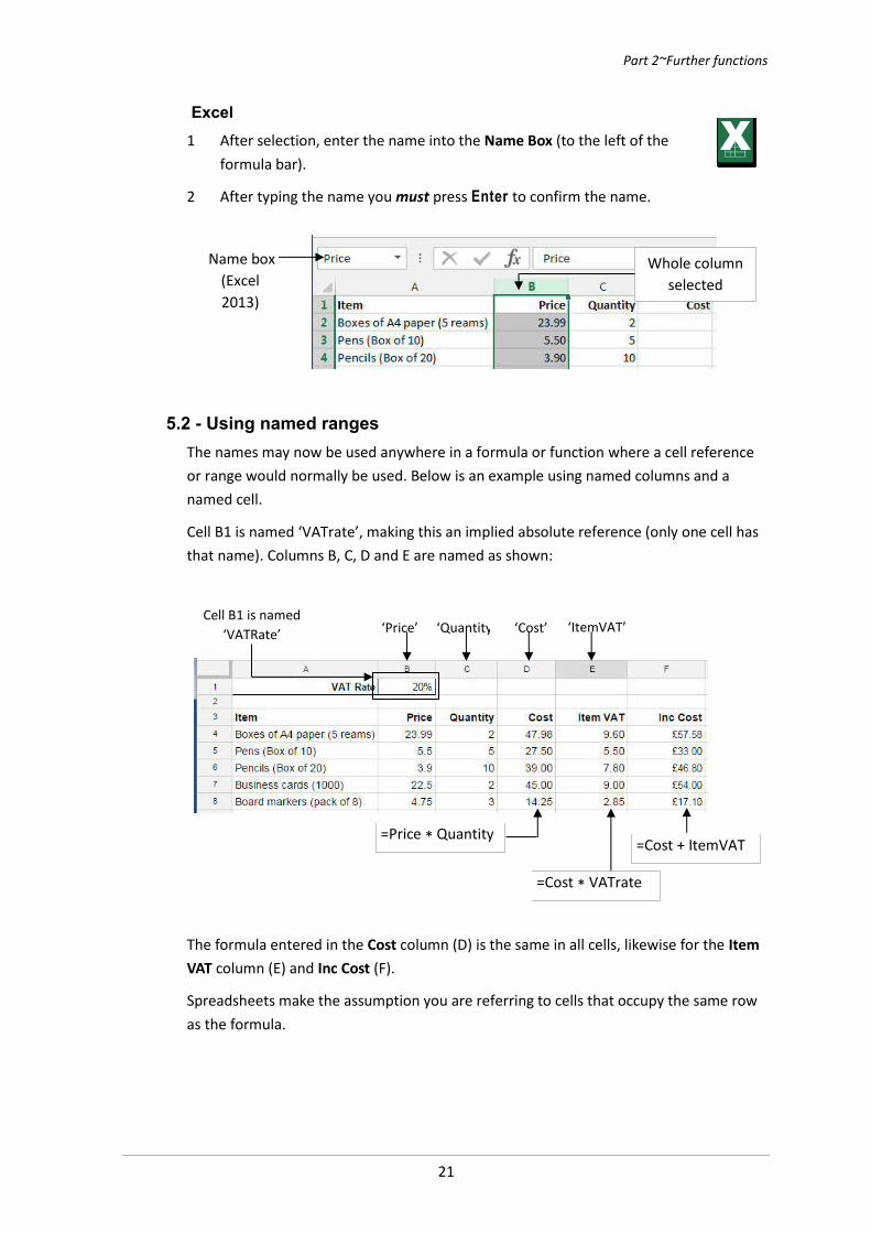
Excel1 After selection, enter the name into the Name Box (to the left of the

formula bar).

2 After typing the name you must press Enter to confirm the name.

5.2 - Using named rangesThe names may now be used anywhere in a formula or function where a cell reference or range would normally be used. Below is an example using named columns and a named cell.

Cell B1 is named ‘VATrate’, making this an implied absolute reference (only one cell has that name). Columns B, C, D and E are named as shown:

The formula entered in the Cost column (D) is the same in all cells, likewise for the Item VAT column (E) and Inc Cost (F).

Spreadsheets make the assumption you are referring to cells that occupy the same row as the formula.

Name box(Excel 2013)

Whole column selected

‘Price’ ‘Quantity’ ‘Cost’ ‘ItemVAT’Cell B1 is named

‘VATRate’

=Price * Quantity

=Cost * VATrate

=Cost + ItemVAT

22

Entering namesSimply type in the name where you would normally enter the cell or range in a formula.

In Excel, a few other options are available:

When you start typing the name, a list of available functions and names (with a label icon) are presented – choose the name (double-click)

Select the cell by name from the name drop-down If a single cell is named, ‘point and click’ will give the name If a column/row is named, ‘point and click’ on the column letter/row number

Note In a Google spreadsheet, clicking on a cell while entering a formula will always give the cell address, not its name.

Managing named rangesTo list all named cells/ranges in the current spreadsheet and to edit/delete them:

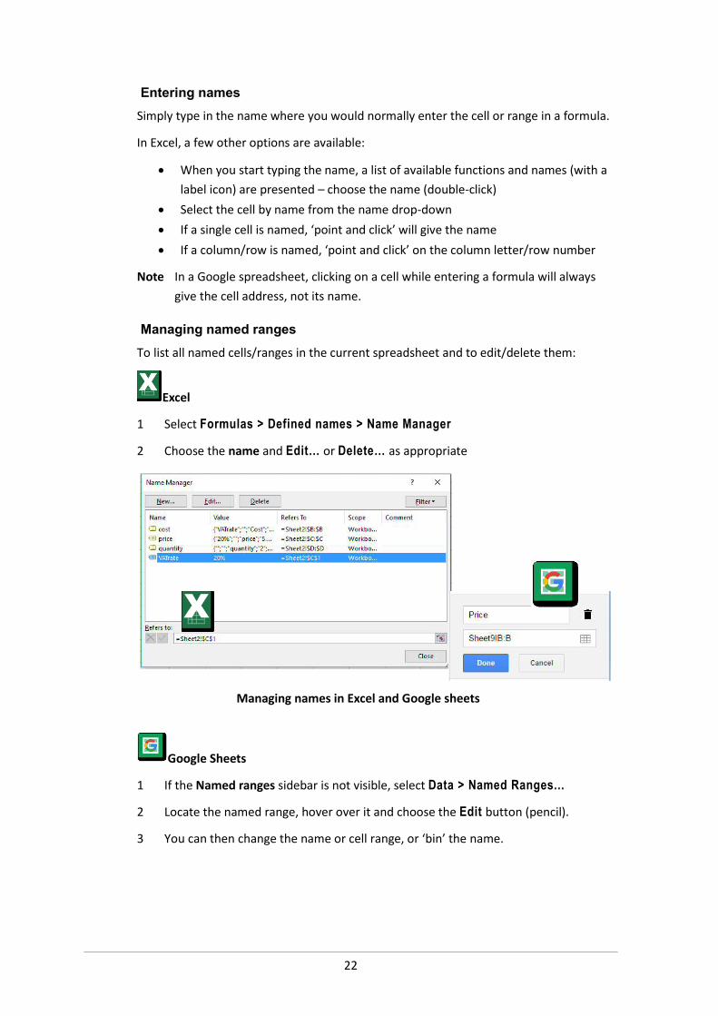
Excel

1 Select Formulas > Defined names > Name Manager

2 Choose the name and Edit… or Delete… as appropriate

Google Sheets

1 If the Named ranges sidebar is not visible, select Data > Named Ranges...

2 Locate the named range, hover over it and choose the Edit button (pencil).

3 You can then change the name or cell range, or ‘bin’ the name.

Managing names in Excel and Google sheets


23

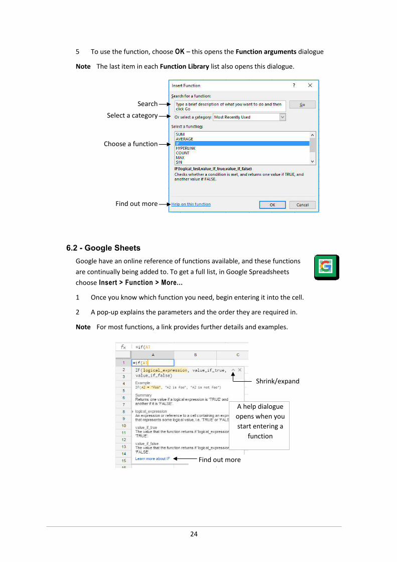
6 ~ Finding and inserting functionsOne way of entering a function is to type it directly into the cell, but this requires that you know the syntax for that particular function. Both Excel and Google Sheets try to help with this in different ways.

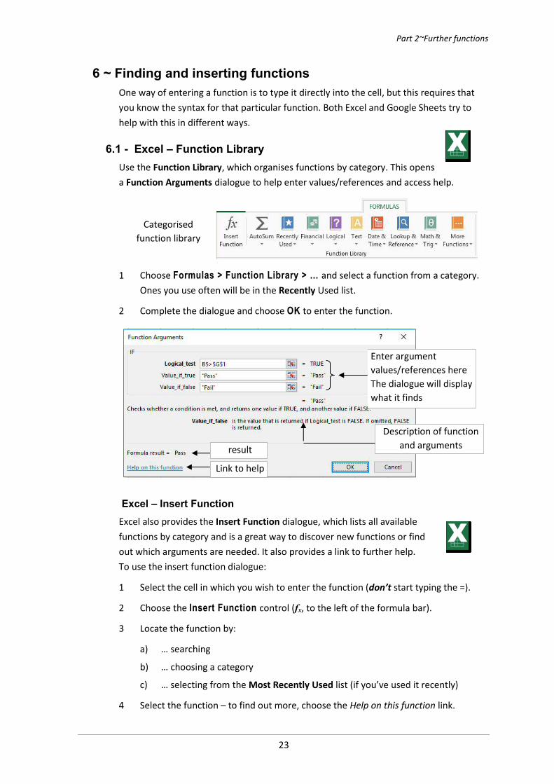
6.1 - Excel – Function LibraryUse the Function Library, which organises functions by category. This opens a Function Arguments dialogue to help enter values/references and access help.

1 Choose Formulas > Function Library > … and select a function from a category. Ones you use often will be in the Recently Used list.

2 Complete the dialogue and choose OK to enter the function.

Excel – Insert FunctionExcel also provides the Insert Function dialogue, which lists all available functions by category and is a great way to discover new functions or find out which arguments are needed. It also provides a link to further help.To use the insert function dialogue:

1 Select the cell in which you wish to enter the function (don’t start typing the =).

2 Choose the Insert Function control (fx, to the left of the formula bar).

3 Locate the function by:

a) … searching

b) … choosing a category

c) … selecting from the Most Recently Used list (if you’ve used it recently)

4 Select the function – to find out more, choose the Help on this function link.

Categorised function library

Enter argument values/references hereThe dialogue will display what it finds

Link to help

result

Description of function and arguments

24

5 To use the function, choose OK – this opens the Function arguments dialogue

Note The last item in each Function Library list also opens this dialogue.

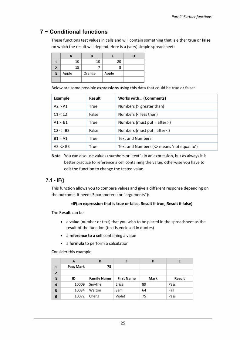
6.2 - Google SheetsGoogle have an online reference of functions available, and these functions are continually being added to. To get a full list, in Google Spreadsheets choose Insert > Function > More...

1 Once you know which function you need, begin entering it into the cell.

2 A pop-up explains the parameters and the order they are required in.

Note For most functions, a link provides further details and examples.

Search Select a category

Choose a function

Find out more

Find out more

A help dialogue opens when you start entering a

function

Shrink/expand


25

7 ~ Conditional functionsThese functions test values in cells and will contain something that is either true or falseon which the result will depend. Here is a (very) simple spreadsheet:

A B C D1 10 10 202 15 7 83 Apple Orange Apple

Below are some possible expressions using this data that could be true or false:

Example Result Works with… (Comments)

A2 > A1 True Numbers (> greater than)

C1 < C2 False Numbers (< less than)

A1>=B1 True Numbers (must put = after >)

C2 <= B2 False Numbers (must put =after <)

B1 = A1 True Text and Numbers

A3 <> B3 True Text and Numbers (<> means ‘not equal to’)

Note You can also use values (numbers or “text”) in an expression, but as always it is better practice to reference a cell containing the value, otherwise you have to edit the function to change the tested value.

7.1 - IF()This function allows you to compare values and give a different response depending on the outcome. It needs 3 parameters (or “arguments”):

=IF(an expression that is true or false, Result if true, Result if false)

The Result can be:

a value (number or text) that you wish to be placed in the spreadsheet as the result of the function (text is enclosed in quotes)

a reference to a cell containing a value

a formula to perform a calculation

Consider this example:

A B C D E1 Pass Mark 7523 ID Family Name First Name Mark Result4 10009 Smythe Erica 89 Pass5 10034 Walton Sam 64 Fail6 10072 Cheng Violet 75 Pass

26

To indicate whether each student had passed, cells in column E would contain an IFfunction to test if the Mark (column D) has reached the pass mark (cell B1).In cell E4 this would be:

You may find it helpful to think of this in terms of a decision tree:

Note There is another solution to this that tests if the Mark is greater than or equal to than the pass mark. Assuming we name cell B1 as passMark, this becomes

=IF(D4 >= passMark,”Pass”,”Fail”)

It doesn’t matter which you use, but it helps to be consistent.

Nesting IFSuppose there are 3 possible outcomes to an exam:

<60 Fail Since one IF function only has two outcomes, it cannot give all 3 possibilities. However, combining two IFfunctions, one inside another, lets you test for all 3 results.

60-80 Pass

>80 Distinction

The decision flowchart now looks like this:

=IF(D4 < passMark,”Fail”,”Pass”)

Test: Is mark in D4 < B1?(cell B1 is named passMark) If true: give result Fail

If false: give result Pass

D4 < B1

= IF…

True

“Pass” “Fail”

False

True

True

False

False

A1 < 60

= IF…

“Pass”

“Fail”

A1 > 80

“Distinction”

IF…


27

The first test can be done with the following function:

=IF(A1<60, “fail”, “pass or distinction”)

This will identify marks that are a fail, but if the result is false, we need now to testbetween a pass and a distinction. To do this we insert the second IF:

=IF(A1<60, “fail”, IF(A1>80, “distinction”, “pass”))

Notes The second IF is not preceded by an equal sign =

While this approach of nesting multiple IF functions could be extended further, it is not advisable for more than a few possible outcomes. Using range lookups is simpler in these cases (see later).

Nesting can be applied with any functions and is a very powerful technique; however the formulae involved can become confusing. Always test your formula carefully to make sure you get the expected results.

7.2 - Conditional COUNT, SUM and AVERAGEThere are several functions which combine sum(), average() and count() with the power of conditional tests. This means cell values will only be counted, totalled or averaged if they meet defined conditions.

These functions require several arguments:

A range of cells to test against the criterion

A value or expression to test against

Optional – a range of cells to SUM or AVERAGE (not for COUNT)

Multiple-criteria versions will also need additional ranges and criteria

Defining arange

Start:End cell references (A2:C32)

Entire column (B:B) or row (5:5)

Several columns (C:E) or rows (5:8)

One or more columns, omitting row 1 (A2:D) (Google only)

A named range

Options for criterion

This can be: A single value

A reference to a cell containing a single value

A reference to a cell containing both value and condition

Note When more than one range is used in a function, they must cover the same number or rows.

28

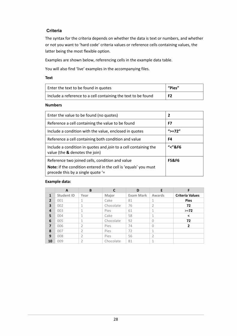
CriteriaThe syntax for the criteria depends on whether the data is text or numbers, and whether or not you want to ‘hard code’ criteria values or reference cells containing values, the latter being the most flexible option.

Examples are shown below, referencing cells in the example data table.

You will also find ‘live’ examples in the accompanying files.

Text

Enter the text to be found in quotes “Pies”

Include a reference to a cell containing the text to be found F2

Numbers

Enter the value to be found (no quotes) 2

Reference a cell containing the value to be found F7

Include a condition with the value, enclosed in quotes “>=72”

Reference a cell containing both condition and value F4

Include a condition in quotes and join to a cell containing the value (the & denotes the join)

“<”&F6

Reference two joined cells, condition and valueNote: if the condition entered in the cell is ‘equals’ you must precede this by a single quote ‘=

F5&F6

Example data:

A B C D E F1 Student ID Year Major Exam Mark Awards Criteria Values2 001 1 Cake 81 1 Pies3 002 1 Chocolate 76 2 724 003 1 Pies 61 1 >=72 5 004 1 Cake 58 1 <6 005 1 Chocolate 92 0 727 006 2 Pies 74 0 28 007 2 Pies 72 19 008 2 Pies 56 2

10 009 2 Chocolate 81 1


29

COUNTIF

COUNTIF(range,criterion) Count the cells in the range that match the criterion

SUMIFThere are two different ways to use SUMIF, depending on whether the values you want to total are also the values you need to test. This means you can total cells in one column depending on values in another column meeting specified criteria:

=sumif(range, criterion) Sums the cells in the range that match the criterion

=sumif(test range, criterion, total range)

Tests the values in the rest range against the criterion, and for each row that matches totals the corresponding values found in the total range

AVERAGEIFThere are two different ways to use AVERAGEIF, depending on whether the values you want to average are also the values you need to test or not. This means you can average cells in one column depending on values in another column meeting specified criteria:

=averageif(range, criterion) Averages the cells in the range that match the criterion

=averageif(test range, criterion, total range)

Tests the values in the rest range against the criterion, and for each row that matches averages the corresponding values found in the total range

7.3 - Multiple criteria with COUNT, SUM and IFThere are also variations of conditional formulae that allow for multiple criteria. These ‘plural’ versions are COUNTIFS, SUMIFS and AVERAGEIFS.

All three functions use pairs of criterion ranges and criteria, but in the case of sum and average you must first also define the range to use for the calculation.

=countifs(range1, criterion1, range2, criterion2 etc)

Counts the number of rows that meet all the defined criteria in all the defined criteria ranges

=sumifs(total range, criterion range1, criterion1, criterion range2, criterion2 etc)

Totals the rows in total range that meet all the defined criteria in all the defined criteria ranges

=averageifs(average range, criterion range1, criterion1, criterion range2, criterion2 etc)

Totals the rows in total range that meet all the defined criteria in all the defined criteria ranges

30

8 ~ Time and date calculationsSpreadsheets store dates and times as formatted numbers.

Dates Dates are stored as a single whole number. Excel starts with 1 in 1900, but Google Sheets permits negative values, allowing pre-1900 dates.Note The first two months of 1900 differ between Excel and Google

Sheets. This is because Excel replicates an error first introduced by Lotus 123 in which 1900 is regarded as a leap year (it wasn’t) and so includes 29/2/1900.All dates after 28 February 1900 agree.

Times Times are stored as decimals – 0.5 is 12 noon

Using this approach means:

A combined date and time can be stored as 1 value

You can perform calculations with dates and times

Note It is up to you to ensure these numbers are formatted appropriately.

8.1 - DatesAdding and subtracting days (format result as a date):

A B C D1 Start date Days End date2 Duck conference 01/01/15 8 = B2 + C2 3 Cake conference = D3 – C3 7 21/01/15

Number of days between two dates (format result as a number):

A B C D1 Start date End Date Duration2 Tree conference 01/01/15 05/01/15 = C2 – B23 Pie conference 14/01/15 20/01/15 = C3 – C2

8.2 - Times and DurationBy default, times will be treated as a time of day, so 12:00 means mid-day. Time can also be used as duration, and used to calculate new times, even on a new day:

A B C D1 Start time Duration New time2 Tree conference 12:00 2:00 14:00 = B2 + C23 Pie conference 21:00 5:30 02:30 = B3 + C3

In some cases, there is no need to distinguish between time and duration. However, unexpected results may occur when totalling durations that exceed 24 hours.

In this case, the cell(s) involved must be formatted as duration. The method used differs between Excel and Google Sheets:


31

Formatting for duration – Google Sheets

Select the cell(s) and choose Format > Number > Duration.

Alternatively, set a custom format (Format > Number > More formats…)

Formatting for duration – Excel

1 Select the cells, choose Home > Number > Number format (drop-down) and select Format Cells… (or right-click and choose Format cells…)

2 Select Custom from the Category list

3 Locate and select the format [h]:mm:ss and OK

Note The square bracket [h] is the important bit

8.3 - Date and Time functions

TODAY() and NOW()Spreadsheets include some functions that are able to refer to the computer’s internal calendar and clock. These functions are unusual in that they require no arguments:

= TODAY() returns the current date (changes when spreadsheet is opened on a new day)

= NOW() returns both the current date and time as a single value (time updates whenever a change is made to the spreadsheet)

Note These values change with the day/time, so cannot be used as a date/time stamp.

Calculations

These functions can be used in calculations, for example to find out how many days there are until a deadline is due:

A B C D1 Project Deadline Days to deadline2 Cake bake 31/05/18 =B3-today()3

Other data and time functionsSeveral other functions allow you to deconstruct and reconstruct date or time values:

=Year(ref), =Month(ref), =Day(ref)=weekday(ref, type)

Generate single integer values for the year, month, day of the month and day of the week (‘type’ determines which is considered day 1)

=Date(ref1,ref2,ref3) Generates a date value from three separate values for year, month and day

=Hour(ref), =Minute(ref), = Second(ref)

Generate single integer values for the hours, minutes and seconds

32

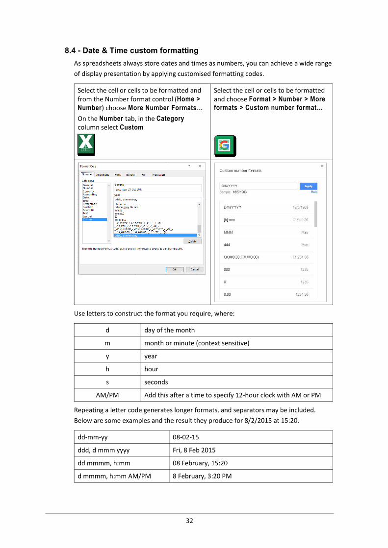
8.4 - Date & Time custom formattingAs spreadsheets always store dates and times as numbers, you can achieve a wide range of display presentation by applying customised formatting codes.

Select the cell or cells to be formatted and from the Number format control (Home > Number) choose More Number Formats…On the Number tab, in the Categorycolumn select Custom

Select the cell or cells to be formatted and choose Format > Number > More formats > Custom number format…

Use letters to construct the format you require, where:

d day of the month

m month or minute (context sensitive)

y year

h hour

s seconds

AM/PM Add this after a time to specify 12-hour clock with AM or PM

Repeating a letter code generates longer formats, and separators may be included. Below are some examples and the result they produce for 8/2/2015 at 15:20.

dd-mm-yy 08-02-15

ddd, d mmm yyyy Fri, 8 Feb 2015

dd mmmm, h:mm 08 February, 15:20

d mmmm, h:mm AM/PM 8 February, 3:20 PM


33

9 ~ Other useful functionsThe range of spreadsheet functions is very extensive, and if you have specific needs it’s worth investigating further what’s available. This section pulls together a few functions that you may find useful in several contexts.

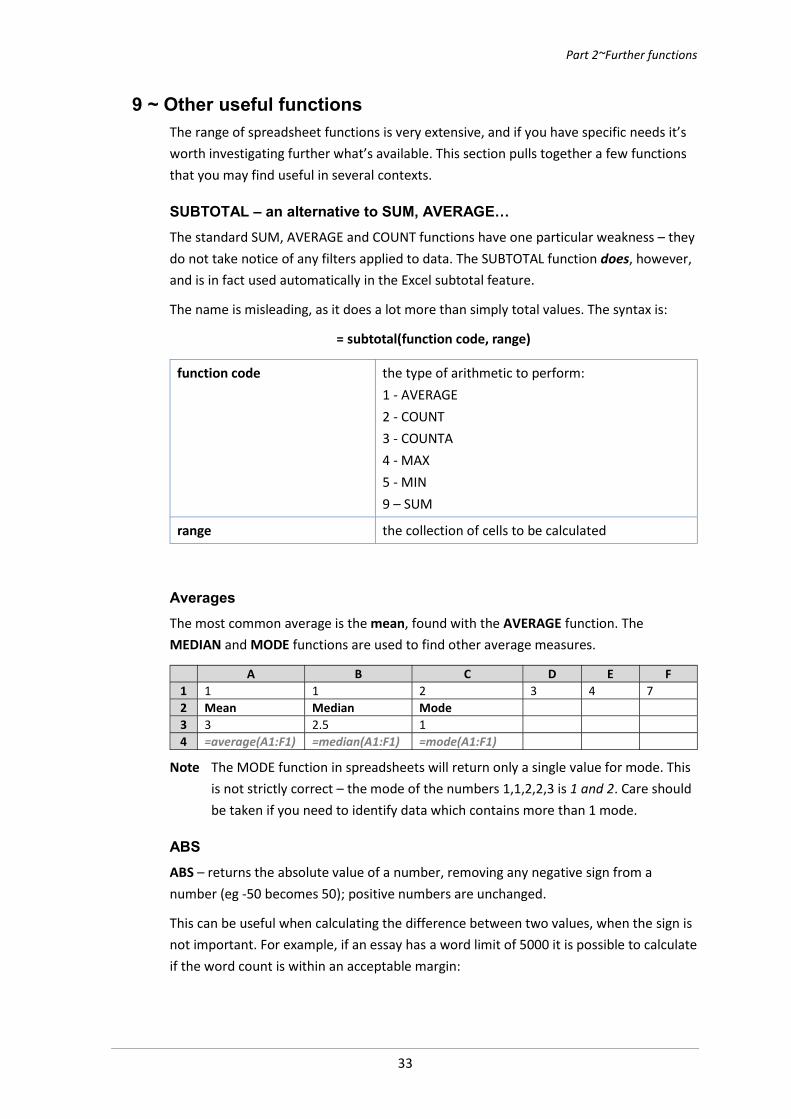
SUBTOTAL – an alternative to SUM, AVERAGE…The standard SUM, AVERAGE and COUNT functions have one particular weakness – they do not take notice of any filters applied to data. The SUBTOTAL function does, however, and is in fact used automatically in the Excel subtotal feature.

The name is misleading, as it does a lot more than simply total values. The syntax is:

= subtotal(function code, range)

function code the type of arithmetic to perform:1 - AVERAGE2 - COUNT3 - COUNTA4 - MAX5 - MIN9 – SUM

range the collection of cells to be calculated

AveragesThe most common average is the mean, found with the AVERAGE function. The MEDIAN and MODE functions are used to find other average measures.

A B C D E F1 1 1 2 3 4 72 Mean Median Mode3 3 2.5 14 =average(A1:F1) =median(A1:F1) =mode(A1:F1)

Note The MODE function in spreadsheets will return only a single value for mode. This is not strictly correct – the mode of the numbers 1,1,2,2,3 is 1 and 2. Care should be taken if you need to identify data which contains more than 1 mode.

ABSABS – returns the absolute value of a number, removing any negative sign from a number (eg -50 becomes 50); positive numbers are unchanged.

This can be useful when calculating the difference between two values, when the sign is not important. For example, if an essay has a word limit of 5000 it is possible to calculate if the word count is within an acceptable margin:

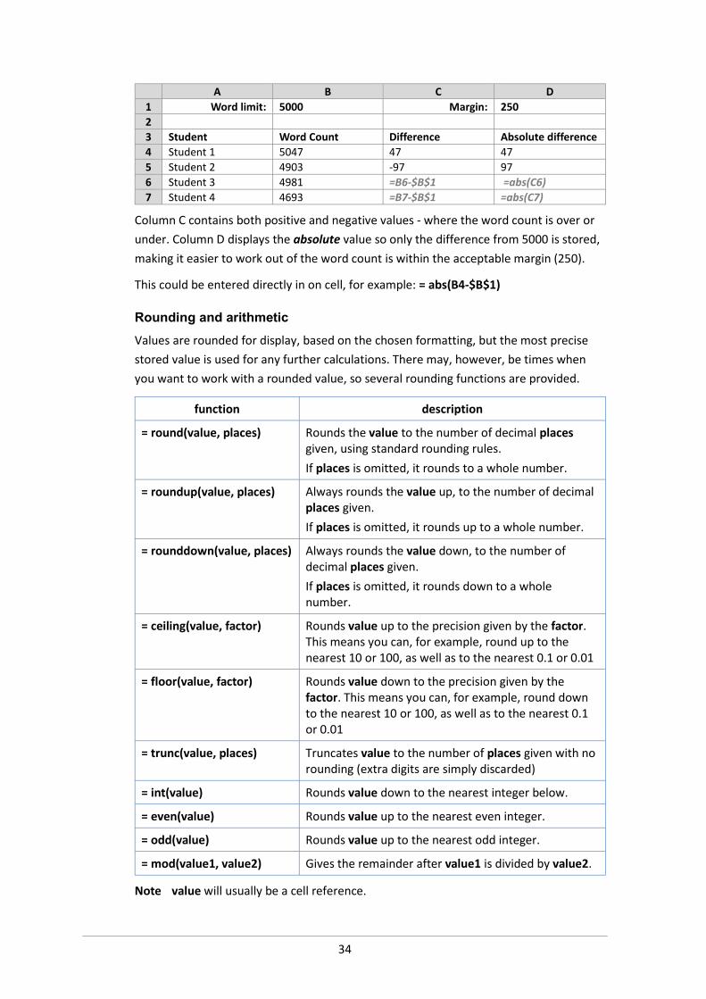
34

A B C D1 Word limit: 5000 Margin: 25023 Student Word Count Difference Absolute difference4 Student 1 5047 47 475 Student 2 4903 -97 976 Student 3 4981 =B6-$B$1 =abs(C6)7 Student 4 4693 =B7-$B$1 =abs(C7)

Column C contains both positive and negative values - where the word count is over or under. Column D displays the absolute value so only the difference from 5000 is stored, making it easier to work out of the word count is within the acceptable margin (250).

This could be entered directly in on cell, for example: = abs(B4-$B$1)

Rounding and arithmeticValues are rounded for display, based on the chosen formatting, but the most precise stored value is used for any further calculations. There may, however, be times when you want to work with a rounded value, so several rounding functions are provided.

function description

= round(value, places) Rounds the value to the number of decimal placesgiven, using standard rounding rules.If places is omitted, it rounds to a whole number.

= roundup(value, places) Always rounds the value up, to the number of decimal places given.If places is omitted, it rounds up to a whole number.

= rounddown(value, places) Always rounds the value down, to the number of decimal places given.If places is omitted, it rounds down to a whole number.

= ceiling(value, factor) Rounds value up to the precision given by the factor. This means you can, for example, round up to the nearest 10 or 100, as well as to the nearest 0.1 or 0.01

= floor(value, factor) Rounds value down to the precision given by the factor. This means you can, for example, round down to the nearest 10 or 100, as well as to the nearest 0.1 or 0.01

= trunc(value, places) Truncates value to the number of places given with no rounding (extra digits are simply discarded)

= int(value) Rounds value down to the nearest integer below.

= even(value) Rounds value up to the nearest even integer.

= odd(value) Rounds value up to the nearest odd integer.

= mod(value1, value2) Gives the remainder after value1 is divided by value2.

Note value will usually be a cell reference.


35

The INT and MOD functions are useful when converting between non-decimal units, eg when converting a number of minutes into hours and minutes:

A B C D1 Minutes Hours Minutes left2 250 4 103 = int(A2/60) = mod(A2/60)

Random numbersThese two random number functions recalculate every time the spreadsheet changes. The ‘randomness’ of the values is probably not good enough for some specialist uses.

=rand() Generates a random decimal number between 0 and 1

=randbetween(low, high) Generates a random integer between low and high. Negative values can be used.

TextSeveral functions allow text manipulation, which may be needed if data is not consistent, or is from another source. Text will usually be a cell reference

Case change

= lower(text) Changes text into lower case

= upper(text) Changes text into upper case (‘capitals’)

= proper(text) Changes text into heading case (first letter of each word capitalised)

trimming and splitting

= len(text) Counts the length (number of characters) in text, including spaces

= trim(text) Removes any leading or trailing spaces from text –data exported from other systems may contain these

= split(text, “delimiter”)

Google sheets only

Splits text into separate cells at each occurrence of the delimiter. If you use more than one character as the delimiter, it uses them separately, not combined.If the delimiter is not a cell reference, it must be enclosed in quotes

= split(text, “delimiter”, false)

Google sheets only

Splits text into separate cells at each occurrence of the delimiter. If you use more than one character as the delimiter, it only splits where they are found together.If the delimiter is not a cell reference, it must be enclosed in quotes

= join(“delimiter”, range) Joins together the content of cells in the range, using the delimiter between them.

36

Google sheets only If the delimiter is not a cell reference, it must be enclosed in quotes – use “” for no delimiter

= left(text, number) Extracts a number of characters starting from the left-hand end of text (including spaces)

= right(text, number) Extracts a number of characters starting from the right-hand end of text (including spaces)

= mid(text, start, number) Extracts a number of characters from the text, beginning at the start position

There are also several other functions that allow you to search for a collection of characters (a ‘string’) inside another one, or look for exact matches between strings.

Splitting textThere are occasions when several items of text (or words) appear in one cell when they should be split over more than one column. This could be because you have imported values from elsewhere, or two ‘fields’ of data may have been put in one column (eg both forename and surname).

Excel includes a tool for splitting text, whereas Google Sheets provides a function:

Excel

1 Select the cell or cells (or column) that contains the data to be split

2 Select Data > Data Tools > Text to Columns

3 Follow the steps of the dialogue to tell Excel about your data

4 Choose Finished when you’ve obtained the desired result in the preview

This method places the first data after splitting into the existing column.

Google Sheets

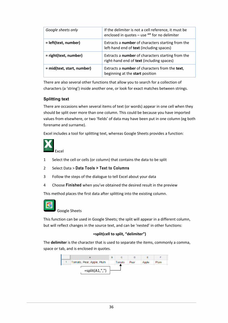
This function can be used in Google Sheets; the split will appear in a different column, but will reflect changes in the source text, and can be ‘nested’ in other functions:

=split(cell to split, “delimiter”)

The delimiter is the character that is used to separate the items, commonly a comma, space or tab, and is enclosed in quotes.

=split(A1,",")

Documents

(VVHQWLDO 6SUHDGVKHHWV %RRN - University of … Excel E} For multiple rows/columns, select the number you wish to insert/delete and proceed as above. $GMXVWLQJURZVKHLJKWDQ GFROXPQZLGWK