HAL Id: hal-00926907https://hal.archives-ouvertes.fr/hal-00926907

Submitted on 10 Jan 2014

HAL is a multi-disciplinary open accessarchive for the deposit and dissemination of sci-entific research documents, whether they are pub-lished or not. The documents may come fromteaching and research institutions in France orabroad, or from public or private research centers.

L’archive ouverte pluridisciplinaire HAL, estdestinée au dépôt et à la diffusion de documentsscientifiques de niveau recherche, publiés ou non,émanant des établissements d’enseignement et derecherche français ou étrangers, des laboratoirespublics ou privés.

Vulnerability of Smart Grids with Variable Generationand Consumption: a System of Systems Perspective

Enrico Zio, Giovanni Sansavini

To cite this version:Enrico Zio, Giovanni Sansavini. Vulnerability of Smart Grids with Variable Generation and Consump-tion: a System of Systems Perspective. IEEE Transactions on Systems, Man and Cybernetics, PartA: Systems and Humans, Institute of Electrical and Electronics Engineers, 2013, 43 (3), pp.477-487.�hal-00926907�

1

Abstract—This paper looks into the vulnerabilities of the

electric power grid and associated communication network, in the

face of intermittent power generation and uncertain demand

within a complex network framework of analysis of smart grids.

The perspective is typical for the system of systems analysis of

interdependencies in a critical infrastructure (CI), i.e. the smart

grid for electricity distribution. We assess how the integration of

the two systems copes with requests to increase power generation

due to enhanced power consumption at a load bus. We define

adequate measures of vulnerability to identify the most limiting

communication time delays. We quantify the probability that a

reduction in the functionality of the communication system yields

a faulty condition in the electric power grid, and find that a

factual indicator to quantify the coupling strength between the

two networks is the frequency of load-shedding actions due to

excessive communication time delay. We evaluate safety margins

with respect to communication specifications, i.e. the data rate of

the network, to comply with the safety requirements in the

electric power grid. Finally, we find a catastrophic phase

transition with respect to this parameter, which affects the safe

operation of the CI.

Index Terms—Complex Networks, System of Systems, Critical

Infrastructures, Smart Grids, Interdependencies, Vulnerability

Analysis, Uncertainty

I. INTRODUCTION

HE life and development of modern Societies is supported

by critical infrastructures (CIs), like the transport and

communication networks or the electrical grid, which grant the

necessary continuous production and distribution of goods and

services [1].

A characteristic of these CIs is that they are highly

interconnected and mutually dependent, i.e. interdependent, in

complex ways, both physically and through information and

communication technologies used for data acquisition and

control, leading to the concept of "systems of systems" [2].

Manuscript received June 21, 2011.

E. Zio is Chair on Systems Science and the Energetic challenge, European

Foundation for New Energy-EDF at Ecole Centrale Paris and Supelec, Paris,

France. He is also with Energy Department, Politecnico di Milano, 20133

Milan, Italy (phone: 39-02-2399.6340; fax: 39-02-2399.6309; e-mail:

enrico.zio@ecp.fr; enrico.zio@supelec.fr; enrico.zio@polimi.it).

G. Sansavini is with Energy Department, Politecnico di Milano, 20133

Milan, Italy (e-mail: giovanni.sansavini@polimi.it).

This brings the need of assessing and controlling the

influences and limitations which interacting CIs impose on

their operating conditions [3].

In particular, a focal subject of interest today is the

evolution of the networks for electrical energy supply and their

conception/renovation as “smart” grids [4]-[8] with distributed

generation, as opposed to the centralized power generation

structure of the existing electric power grids. One key aspect

characterizing smart grids is the combination of the electric

power grid with an information and communication network to

“improve the observability and controllability of the

distribution grid and thereby convert it from a static

infrastructure to be operated as designed to a flexible, dynamic

infrastructure operated proactively” [4].

The concepts and configurations of smart grids vary

sensibly with respect to the implementation at the different

levels of the electrical infrastructure, i.e. the transmission and

distribution systems (the level of the individual costumer, and

the related pricing issues, lies beyond the scope of the study

presented in this paper) [5].

At the level of the transmission system, the efficiency and

stability of power system operation could be improved

substantially by phase angle measurements at many key

locations and the use of Flexible AC Transmission System

control devices (FACTS), combined with distributed and

autonomous control strategies and high-speed communication.

The level of the distribution system is the one usually

referred to when introducing concepts of smart grids. Unlike

the transmission grids that are arranged as meshed networks,

the distribution networks form tree-like, radial structures,

characterized by a central distribution hub where power enters

and is routed to the loads along the parallel branches of the

distribution feeders. If a malfunctioning occurs, circuit

breakers automatically disconnect the entire feeder. The use of

multiple power injection points, and sensors and remote

control switches that can isolate and cut off the problem would

guarantee the continuous power supply to the other buses of

the feeder [9]. Furthermore, at present stage the disconnection

of the entire feeder is the only strategy to balance a load excess

when generation is suddenly lost due to an emergency.

Conversely, a combination of smart meters and advanced

distribution automation would allow controlling individual

loads along a distribution feeder so that critical services (such

Vulnerability of Smart Grids with Variable

Generation and Consumption: a System of

Systems Perspective

Enrico Zio, Senior Member, IEEE, and Giovanni Sansavini

T

2

as police stations, hospitals, emergency services) can remain

connected, while loads that provide less critical services can be

dropped. Furthermore, the deployment of small-size diffuse

generation would relieve stresses on transmission and

distribution systems, and allow the disconnection of the

distribution feeder from the main power system to run it as an

isolated island, serving only a few critical loads in case of an

emergency (this is not currently allowed for technical, legal,

safety, and regulatory reasons).

Irrespective of the system level under consideration, the

smart grid is an auto-balancing, self-monitoring power grid

that has the ability to sense when a part of its system is

overloaded and reroute power to reduce overload and prevent

a potential outage situation. It enables real-time

communication between users and utility, allowing optimal

energy usage, and the introduction of renewable energy

sources for minimizing the collectivity environmental footprint

[4].

The use of renewable energy sources poses challenges to the

design and the operations of the electric power grid. The

availability of these sources is strictly dependent on the

climatic conditions, i.e. cloud cover or wind speed and

steadiness. Then, the power output of solar and wind electric

generators is affected by uncertainty and intermittency [10]-

[12]: paradoxically, due to its intrinsic stochastic nature,

electric power from renewable sources could be abundantly

available when it is not needed, while scarce in other cases of

necessity. Moreover, electrical energy from renewable sources

is typically produced in remote areas, e.g., where strong and

steady winds are available or solar power plants can be

conveniently located. This power has to be routed through the

transmission network and delivered to distant locations where

it is consumed. Yet, the existing power transmission

infrastructure is not currently designed to carry intermittent

electrical flows with possibly large peak flows, and in some

cases it is inadequate to serve new remote power plants. As an

example, a recent study [13] commissioned by the Italian

Association of Energy Producers from Renewable Sources

(APER) has estimated that between 2008 and 2009 the wind

farms located in Southern Italy have lost 700 GWh (25% of

the maximum producible energy) due to the limited current-

carrying capacity of the high-voltage transmission lines and the

scarce power demand in the area near the plants,

corresponding to an economic loss of 144 millions of Euros.

The deployment of small-size renewable power generation

at the electric distribution level is also rapidly changing the

nature of this infrastructure. Traditionally a passive recipient

of a unidirectional flow from the transmission network, the

distribution network should now support injections of active

power from its users. In this perspective, both the transmission

and the distribution networks require a real-time control

approach with an increasing level of complexity due to the

broad space distribution of the generators and to the high

degree of variability that characterizes electrical power from

renewable sources [6].

Electric transmission networks already have some

instrumentation that allows control centers to automatically

monitor power flows and open or close circuit breakers at

substations as a result of human- and computer-generated

control decisions [5]. This communication level is based on

heterogeneous technologies and platforms which are poorly

integrated [14]. On the contrary, distribution networks lack

instruments for the information exchange and the system

control.

Considering the present lack of standards, the

communication network will have to evolve with the

developing Smart Grid. Communication links will need to use

all kinds of resources, varying from hard-wired links to fiber

optics, power line communication [15], wireless [16], satellites

and micro-wave links, in order to serve the large geographical

territory covered by the smart grid [7]. All of these

communication links constitute opportunities but also

introduce vulnerabilities, due to functional failures and

exposition to malevolent attacks aiming at causing system-

wide instabilities and blackouts, especially if they are not

protected in dedicated supports but can be accessed over the

Internet.

The coupling between the electric power and

communication networks in Smart Grids raises safety and

security issues [17]. In the smart grids, the continuous delivery

of electric power is supported by the communication

infrastructure and, vice versa, the exchange of information

relies on the energy input of the electric power grid. Faults

originating in one of the two networks impact on the other

interdependent one. For example, the interruption or even the

delay of the information flow communicating a control action

upon the electric power grid may result in power unbalance

and system instability that could trigger a blackout [7], [18].

Vulnerability analysis must then be concerned with the

interconnected, mutually dependent systems to properly

account for the influences and limitations which the interacting

electrical power grids and communication networks impose on

the individual system operating conditions, for avoiding fault

propagation by designing redundancies and alternative modes

of operations, and by detecting and recognizing threats.

This paper looks into the vulnerabilities of the electric

power grid and associated communication network, in the face

of intermittent power generation and uncertain demand within

a complex network framework of analysis of smart grids.

Complex network approaches for the analysis of distributed

systems [19]-[25] take a holistic perspective in which the

overall system behavior emerges as the result of the complex

interactions of its constituents. The two main objectives of the

analysis are (i) to identify preliminary vulnerabilities by

topology-driven and dynamic analysis, and (ii) to guide and

focus further detailed analyses of critical areas based on

physical codes (e.g. incorporating line impedances and

Kirchhoff's laws to assess the power flows from the generators

to the loads of an electric network). Purely-topological,

complex network models of the electric power grid [19]-[25],

3

which abstract the physical details of the provided service and

characterize the topology of network systems, are here

extended to capture essential operating features, i.e. the power

is routed through the least resistant paths, the components are

physically specialized in “generators” and “distributors”, the

lines are subjected to limits on their carrying-flow capacities

and the power generation and consumption levels vary within a

range of uncertain values.

In order to account for the interdependence effects due to

the coupling [26], we adopt a framework in which the

communication delays are integrated in the electric CI. The

communication network is assumed to be made of dedicated

control signal channels. The coupling between the two

interdependent networks occurs at the components level. Each

node of the electric network is coupled with a router that

ensures communication with the other elements of the network.

The time required to exchange data from the measurement

location to a control center or data concentrator, and the time

required ultimately to communicate these data to the control

devices, is collectively denoted as communication delay or

latency. As stated before, excessive communication delay may

result in power unbalance and system instability that could

trigger a blackout. The calculation method of the

communication delay encompasses several sources, including

routing delays which are modeled as a series of M/M/1 queues,

which symbolizes the cumulative time delay along the routing

path from the measurement site to the control unit [27].

According to the shorthand notation developed for queuing

systems, the three-part descriptor M/M/1 denotes a one-server

queuing system with exponentially-distributed inter-arrival and

service times [28].

We assess the vulnerability of the two interdependent

networks subject to the specific hazard defined by the request

of increase of power generation due to enhanced power

consumption of one load. To this aim, we introduce

vulnerability measures that identify the most critical

communication time delays, and assess the probability that a

reduction in the functionality of the communication system

will generate a faulty condition in the electric power grid.

The paper is organized as follows: the embraced

interpretation of vulnerability is detailed in Section II; the

modeling of the smart grid CI with interdependencies is

presented in Section III; Section III.A describes the model of

power flow in the electrical transmission network and Section

III.B describes the model of information flow in the

communication network; Section III.C details the simulation

procedure devised for analyzing the vulnerabilities of the two

coupled CIs. In Section IV, the proposed model is applied to

two interdependent networks whose structures are based on the

380 kV Italian power transmission network [29], [30], and

Section IV.A discusses the numerical results. Conclusions are

drawn in Section V.

II. VULNERABILITY ANALYSIS OF CRITICAL

INFRASTRUCTURES

While the concept of risk is fairly mature and consensually

agreed, the concept of vulnerability is still evolving and not yet

established. In general terms, risk refers to a combination of

the probability of occurrence of a specific event leading to

loss, damage or injury and its extent. These quantities and their

associated uncertainties are regarded as being numerically

quantifiable.

The term vulnerability has been introduced as the concept of

risk is somehow limited in portraying the hazard-centric

perception of disasters. A hazard of low intensity could have

severe consequences, while a hazard of high intensity could

have negligible consequences: the level of vulnerability is

making the difference [31]. The concept of vulnerability seen

as a global system property focuses on three elements [32]: (i)

degree of loss and damages due to the impact of a hazard; (ii)

degree of exposure to the hazards, i.e., likelihood of being

exposed to hazards of a certain degree and susceptibility of an

element at the risk of suffering loss and damages; (iii) degree

of resilience, i.e., the ability of a system to anticipate, cope

with/absorb, resist and recover from the impact of a hazard or

disaster.

Vulnerability is here interpreted as a flaw in the design,

implementation or operation of an infrastructure system, or its

elements, that renders it susceptible to destruction or

incapacitation when exposed to a hazard or threat, or reduces

its capacity to resume new stable conditions [1], [33]. The

latter can be provided with a likelihood (frequency) while a

measure for destruction or incapacitation needs specific

elaborations. In this study, the vulnerability of the two

interdependent networks is expressed in terms of frequency of

load-shedding actions due to excessive communication time

delay, with respect to several ranges of power increase request.

The goals of vulnerability analysis, and the associated

modeling and simulation efforts, could be: (i) given a system

and the end state of interest, identify the set of events and

event sequences that can cause damages and loss effects; (ii)

identify the relevant set of ‘‘initiating events’’ and evaluate

their cascading impact on a subset of elements, or the system

as a whole; (iii) given a system and the end state of interest,

identify the set of events or respective event sequences that

would cause this effect; (iv) given the set of initiating events

and observed outcomes, determine and elaborate on

(inter)dependencies (within the system and among systems)

and on coupling effects of different orders [1].

The achievement of these goals relies on the analysis of the

system, its parts and their interactions within the system; the

analysis must account for the environment which the system

lives in and operates, and finally for the objectives the system

is expected to achieve. The ultimate goal is to identify the

vulnerabilities for managing and reducing them.

4

III. DYNAMIC MODEL OF INTERDEPENDENT NETWORKS AND

SIMULATION PROCEDURE

The electric power grid and the communication network are

represented by two graphs G1(N1,K1) and G2(N2,K2) with N1,

N2 nodes connected by K1, K2 links, respectively. In our case,

it has been assumed (without loss of generality) that N1=N2=N

and K1=K2=K. The networks are specified by NN adjacency

(connection) matrices whose entries are 1 if there is an edge

joining node i to node j or 0, otherwise, and by connection

length matrices whose entries are the physical length of the

line connecting node i to node j if there is an edge joining node

i to node j or 0, otherwise.

In the electric power grid, the nodes correspond to buses.

They are further specified into NG generators, i.e. the providers

of the service, and ND distributors, i.e. the recipient of the

service. The edges correspond to electrical connections.

In the communication network, the nodes correspond to

routers and the edges to dedicated control signal channels that

connect them.

The interdependencies within the CI are due to the presence

of routers on each electrical bus. Routers send and receive

control commands that try to match the generation profile with

the power demand in the electrical network according to the

increase of electrical load.

The system, then, does not rely on a centralized control

center. Control decisions are locally taken at the router/bus

level and communicated to the other interacting buses/routers

[33]. During this process, the total time required to the system

to balance generation and demand, i.e. the communication

time delay, T, is monitored.

A. The functional model of power flow in the electrical

transmission network

The functional model of the electric power grid abstracts the

physical details while at the same time capturing its essential

operating features. The elements of the network are

characterized by loading values normalized in the interval [0,

1] that identify how close to the limit capacity they are

operating. For generator and distributor nodes, Li [0, 1]

identifies the fraction of maximum power that generator i is

injecting in the network, or alternatively, the fraction of

maximum power that distributor i is absorbing from the

network. The value Li = 1 identifies the maximum power that a

generator i can inject in the system, or alternatively, the

maximum power that distributor i has agreed to receive by

contractual agreement. For lines, Lij [0, 1] identifies the

fraction of the maximum flow-carrying capacity that the line

connecting node i to node j is serving. The value Lij = 1

indicates that the line connecting node i to node j, hereafter

also called line ij, is operating at its maximum flow carrying-

capacity.

The loading scenario is identified when the N values of Li

and the K values of Lij are known. To account for the

variability that characterizes generation and consumption, the

Li values are sampled from uniform probability distributions in

the intervals [LGmin

, LGmax

] for generators and [LDmin

, LDmax

]

for distributors.

We assume that the flow of electrical power from generator

i to distributor j follows the least resistant path between i and j.

We further assume line resistance to be proportional to line

length; hence the least resistant paths and the shortest paths

coincide. We find the shortest paths that connect any generator

i to any distributor j, and rank in descending order the lines

with respect to their participation to the shortest paths. The Lij

values are then also sampled from uniform probability

distributions. In particular, two probability distributions are

assumed that describe two possible states [Llowmin

, Llowmax

] for

lines that are likely to accommodate low values of power, and

[Lhighmin

, Lhighmax

] for lines that are likely to accommodate large

values of power. To this aim, The Lij value is sampled from

[Lhighmin

, Lhighmax

] if line ij belongs to the first half of the rank,

while it is sampled from [Llowmin

, Llowmax

] if line ij belongs to

the second half of the rank. This sampling procedure assigns

on the average a higher power flow to those lines that are

traversed by many generator-distributor shortest paths, i.e. that

have a high betweenness centrality [36].

In the following, we assess how the CI copes with an

increase in the electrical power demand. To this aim, starting

from an initial loading scenario, we simulate a request of

additional power, W, by distributor i. We assume that W is

described by a uniform probability distribution [Wmin

, Wmax

].

The overall load Li + W may also possibly exceed the

maximum contractual power that i has agreed to receive from

the system, i.e. 1.

B. The model of information flow in the communication

network

In [27], Stahlhut et al. assess how the communication delay

for measurements and control signals in a power system

impacts the control system response. In the following, we

embrace their calculation of the communication delay, and

assume that the data transmitted are in the form of packets.

The packets are a formatted block of information and are

typically arranged in three sections: the header, the payload,

and the trailer. The header has the following information:

packet length, origin and destination address, packet type, and

packet number (if a sequence of packets is being sent). The

payload carries the data taken from the measurement. The

trailer is at the end of the packet and carries information which

permits the receiving device to identify the end of the packet.

The time delay calculation encompasses several different

delays that occur in communication systems. These delays

typically are:

• serial delays: the delay of having bits being sent one after

another;

• “between packet” serial delays: the time after a packet is

sent to when the next packet is sent;

• propagation delays: the time required to transmit data over

a particular communication medium;

• routing delays: the time required for data to be sent

through a router, and resent to another location.

5

The total signal time delay may be represented as

s b p rT T T T T (1)

s s rT P D (2)

PT l v (3)

where Ts is the serial delay, Tb is the between packet delay,

Tp is the propagation delay, Tr is the routing delay, Ps is the

size of the packet (bits/packet), Dr is the data rate of the

network, l is the length of the communication medium, and v is

the velocity at which the data are sent through the

communication medium (e.g., 0.6 to c, where c is the speed of

light).

Routers are a major part of the communication

infrastructure in a communication network. There are a

number of methods by which routing delay can be

approximated [37]-[41]. A simple and fast calculation method

of routing delay can be used to approximate the delay at a

router: this calculation method is based on a series of M/M/1

queues [28], in which a path from the measurement to the

control center is traced, and all of the routing delays are added

up to represent the total routing delay for the measurement.

For this calculation,

1

Ni

r r

i

T T

(4)

where Tr is the total routing delay, i

rT is the routing delay

for a single router at location i, and N is the total number of

routers. The M/M/1 queue is used to approximate the value of i

rT for each router i, and it is modeled as a one-server

queuing system with exponentially-distributed inter-arrival and

service times [28]. The M/M/1 queue has several associated

performance measures such as: the average number of

customers in line, the average number of customers in the

system, the time waiting in line, and the time required to pass

through the system [39], [42]. In this context, the customers

are the sensory messages in the communication network. A

noteworthy performance measure is the total waiting time

(system time), and this encompasses both the amount of time

waiting in line (waiting time), as well as the amount of time

being served (service time). The total waiting time is

quantified as

(5)

where is the rate at which objects come in the system

(e.g., packets/s) and µ is the rate at which the objects are being

served (e.g., packets/s). The routing time i

rT for each router i

can be estimated from (5) and used in (4) to calculate the total

routing delay

1

iN

r i i ii

T

(6)

We assume that information from router i to router j flows

along the shortest path connecting i and j. Therefore, the total

routing time, Tr, from router i to router j is evaluated as the

sum of the routing delays of the encountered routers along the

shortest path connecting i and j.

The maximum time delay that the smart grid can tolerate

depends on the system task to be executed and ranges from

tenths of milliseconds up to tenths of seconds [6], [7]. For

example, the standard specifies that for an unintentional island

in which the distributed generation energizes a portion of the

distribution network, the control system shall detect the island

and cease to energize the portion within 2s of the formation of

an island. Moreover, latencies in the tens of ms allow rapid

detection of faults and are the accepted fault detection times

[7]. On the contrary, voltage and active power regulation

actions should be accomplished within 10s and some minutes,

respectively [6].

C. Simulation procedure

To test the vulnerability of the CI with respect to the

stability upon a power increase request, W, we proceed in

successive stages as follows:

1. All N components of the electric power grid are working

under independent uniformly random initial loads. In

particular, Li [LG

min, LG

max] for generator i = 1,…NG, L

i

[LDmin

, LDmax

] for distributor i = 1+ NG,…ND + NG, and Lij

[Lhighmin

, Lhighmax

], or Lij [Llow

min, Llow

max], if line ij

belongs to the first or second half of the betweenness

centrality rank (Section III.A), respectively, i , j = 1,…, N.

These values identify the loading scenario.

2. A distributor node i is chosen randomly and its power

demand is increased from Li to L

i + W, where W is sampled

from the uniform probability distribution [Wmin

, Wmax

].

3. The NG generators that are connected to i are sorted by

ascending distance from i, i.e. ascending resistance. The

closest generator j = 1 is selected. Communication delay T is

set to zero.

4. Distributor i queries generator j for additional power W.

Generator j answers providing the value of the power

available to i, i.e. min ,1 jSG j W L , where 1 - Lj is

the maximum additional power that j can provide.

Communication time delay, T, is updated.

5. Check whether the shortest path between i and j can

accommodate the additional power SG(j). To this aim, every

line yz on the shortest path between i and j is tested for

infringement of the current-carrying capacity limit in the

new configuration, i.e. Lyx

+ SG(j) 1. If at least one limit is

exceeded the additional power is updated to the maximum

power value that satisfies all the line constraints, i.e.

6

min 1 yz

yzSG j L , for every line yz on the shortest path

between distributor i and generator j, SG(j) = 0 in case that a

line yz is already operating at its maximum flow-carrying

capacity. The residual power that distributor i still requires,

U(i), and the power that generator j could not supply, UG(j),

are evaluated as 1

( )j

s

U i UG j W SG s

. They are

recorded for the vulnerability evaluation. Communication

time delay, T, is updated.

6. The generator index j is incremented by 1, and the

procedure is returned to step 4 until U(i) = 0, in case of a

successful system state, or j = NG and U(i) > 0, in case the

power request is not satisfied. The final communication time

delay, T, is recorded.

The value of U(i) at the end of the simulation is the fraction

of the additional load W that has to be shed in order to balance

the power generation and the power consumption. Therefore,

we assume that load can be continuously shed.

Furthermore, it can be noticed that the power that generator

j could not supply, UG(j) can be greater than 0 for two

different causes: either j is operating at its maximum capacity,

or there is no path for the power produced by j for reaching the

distributor i where it is needed. This feature of the algorithm is

consistent with the behavior of smart grids that include

intermittent and remotely-generated electricity from renewable

energy sources, as discussed in Section I.

To incorporate the effects of load and generation

uncertainties, the above algorithm is embedded in a Monte

Carlo simulation framework, in which a large number of

additional load requests, e.g., 100000 in this study, is

simulated for the same range of [LGmin

, LGmax

], [LDmin

, LDmax

],

[Lhighmin

, Lhighmax

], [Llowmin

, Llowmax

] and [Wmin

, Wmax

], in order to

obtain statistically significant results for various realizations of

the same average loading condition.

During the simulations, relevant statistics are recorded to

evaluate different vulnerability indexes, i.e. the distribution of

the communication time delay, T, in case of a successful (no

load-shedding is required to balance consumption and

generation) or unsuccessful (load-shedding is required to

balance consumption and generation) final system state.

The effects of the interdependencies between the electric

power grid and the communication network are evaluated with

respect to the communication time delay, T , that elapses from

the instant in which the request for power increase is done,

until the request is fulfilled. As seen in Section III.B, the

maximum time delay requirements, TMAX

, for the smart grid

range from tenths of milliseconds up to tenths of seconds

depending on the system task to be executed. In this respect,

various communication network configurations differing for

the value of the data rate, Dr, can be tested to quantify the

probability that a malfunction in the communication system,

i.e. a communication delay, will generate a faulty condition in

the electric power grid. The compliance with TMAX

, i.e. T <

TMAX

, is evaluated at the end of the simulations.

IV. CASE STUDY

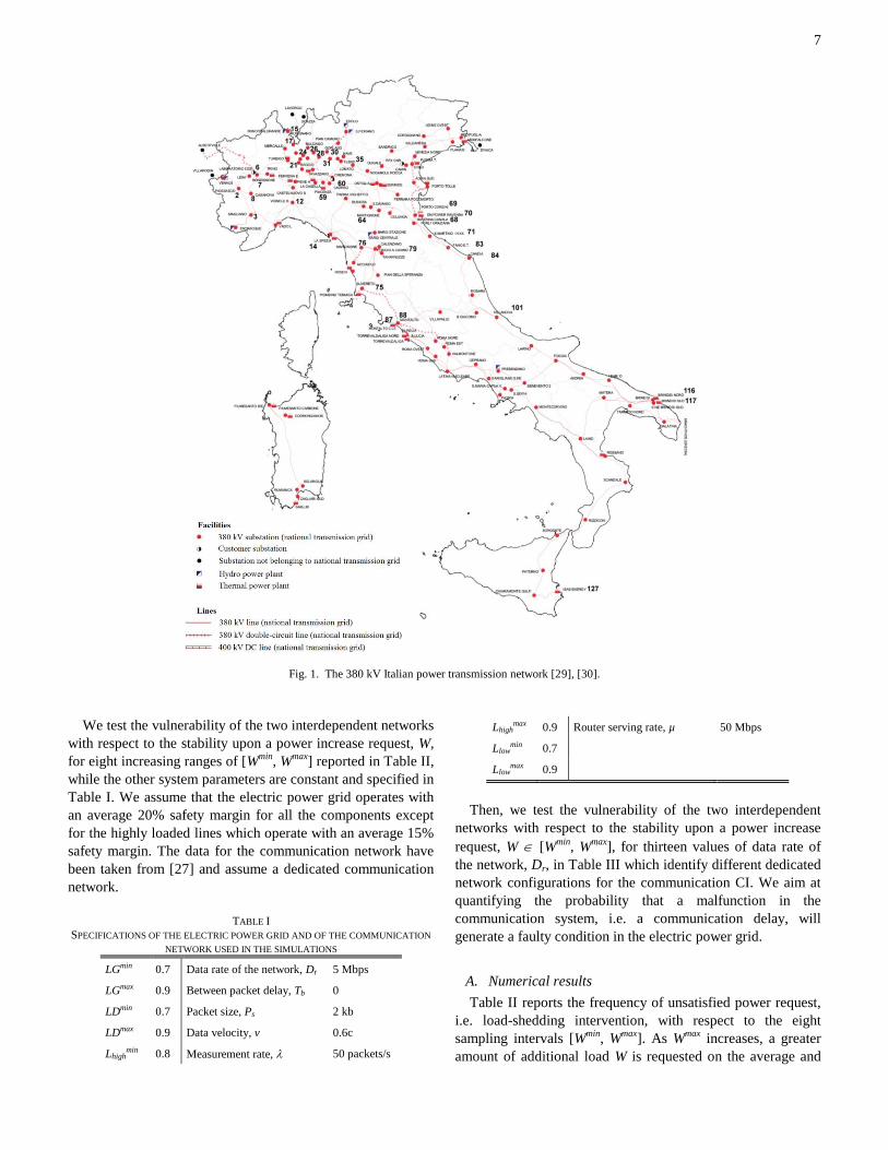
The approach to evaluate the vulnerability of the smart grid

CI with interdependencies between power and communication

networks introduced in Section III, is exemplified with

reference to the topological network of the 380 kV Italian

power transmission network (Fig. 1), focusing only on its

structure with no further reference on the electrical properties,

coupled with a dedicated communication network. For

simplicity, but with no loss of generality, we assume that the

two networks have the same topologies. The developed

methodology can be applied to interdependent networks with

different topologies. The 380 kV Italian power transmission

network is a branch of a high voltage level transmission, which

can be modeled as a network of N=127 nodes (NG=30

generator and ND=97 distributor nodes) connected by K=171

links [29], [30], defined by its N×N adjacency (connection)

matrix aij and connection length matrix lij. We assume that the

communication network consists of dedicated control signal

channels, which follow the same layout of the overhead

electrical lines. Therefore, both the electric power grid and the

communication network are described by the same aij and lij

matrices (without loss of generality): the topology and the

geographical location of the 380 kV Italian power transmission

network components serve as reference.

7

Fig. 1. The 380 kV Italian power transmission network [29], [30].

We test the vulnerability of the two interdependent networks

with respect to the stability upon a power increase request, W,

for eight increasing ranges of [Wmin

, Wmax

] reported in Table II,

while the other system parameters are constant and specified in

Table I. We assume that the electric power grid operates with

an average 20% safety margin for all the components except

for the highly loaded lines which operate with an average 15%

safety margin. The data for the communication network have

been taken from [27] and assume a dedicated communication

network.

TABLE I

SPECIFICATIONS OF THE ELECTRIC POWER GRID AND OF THE COMMUNICATION

NETWORK USED IN THE SIMULATIONS

LGmin 0.7 Data rate of the network, Dr 5 Mbps

LGmax 0.9 Between packet delay, Tb 0

LDmin 0.7 Packet size, Ps 2 kb

LDmax 0.9 Data velocity, v 0.6c

Lhighmin 0.8 Measurement rate, 50 packets/s

Lhighmax 0.9 Router serving rate, µ 50 Mbps

Llowmin 0.7

Llowmax 0.9

Then, we test the vulnerability of the two interdependent

networks with respect to the stability upon a power increase

request, W [Wmin

, Wmax

], for thirteen values of data rate of

the network, Dr, in Table III which identify different dedicated

network configurations for the communication CI. We aim at

quantifying the probability that a malfunction in the

communication system, i.e. a communication delay, will

generate a faulty condition in the electric power grid.

A. Numerical results

Table II reports the frequency of unsatisfied power request,

i.e. load-shedding intervention, with respect to the eight

sampling intervals [Wmin

, Wmax

]. As Wmax

increases, a greater

amount of additional load W is requested on the average and

8

the generators closest to the increasing load cannot provide the

total required amount. Thus, distant generators are queried, but

power cannot always find a path to reach the increasing load

due to growing likelihood of line limit infringement along the

path, and the system has little chances to fully satisfy W.

TABLE II

FREQUENCY OF UNSATISFIED POWER REQUEST, I.E. LOAD-SHEDDING

INTERVENTION, AND THE ASSOCIATED STANDARD ERROR VS. THE WIDTHS OF

THE EIGHT UNIFORM SAMPLING INTERVALS FOR THE ADDITIONAL POWER, W.

THE NUMBER OF SIGNIFICANT DIGITS THAT WE REPORT THROUGHOUT THE

PAPER IS EVALUATED BY YONEDA’S RULE [43].

Sampling interval for the

additional power request, W

Frequency of

unsatisfied request Standard error

[0.10, 0.15] 0.6670 % 0.1252 %

[0.10, 0.20] 1.1950 % 0.1263 %

[0.10, 0.25] 2.6000 % 0.1717 %

[0.10, 0.30] 6.565 % 0.384 %

[0.10, 0.35] 11.788 % 0.316 %

[0.10, 0.40] 17.587 % 0.554 %

[0.10, 0.45] 23.083 % 0.425 %

[0.10, 0.50] 28.835 % 0.553 %

[Fig. 2-7 in the previous manuscript were removed in order

to comply with the 12 page limit for IEEE Transactions on

Systems, Man and Cybernetics, Part A –Systems and Humans

regular papers. Table 3-6 in the previous manuscript were

removed in order to comply with the 12 page limit for IEEE

Transactions on Systems, Man and Cybernetics, Part A –

Systems and Humans regular papers. The comments to the

removed results were also removed.]

The frequency of unsatisfied power request in Table II

characterizes the self-limitations that the electric power grid

imposes on its own operations due to its structural

configuration, the limits on flow-carrying capacities of lines,

the intermittent nature of power generation from renewable

energy sources and the uncertainties in the load demand

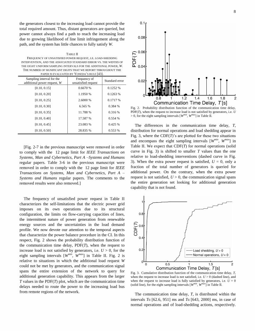
profile. We now devote our attention to the temporal aspects

that characterize the power balance procedure in the CI. In this

respect, Fig. 2 shows the probability distribution function of

the communication time delay, PDF(T), when the request to

increase load is not satisfied by generators, i.e. U > 0, for the

eight sampling intervals [Wmin

, Wmax

] in Table II. Fig. 2 is

relative to situations in which the additional load request W

could not be met by generators, and the communication signal

spans the entire extension of the network to query for

additional generation capability. This appears from the larger

T values in the PDF(T) plot, which are the communication time

delays needed to route the power to the increasing load bus

from remote regions of the network.

Fig. 2. Probability distribution function of the communication time delay,

PDF(T), when the request to increase load is not satisfied by generators, i.e. U

> 0, for the eight sampling intervals [Wmin, Wmax] in Table II.

The differences in the communication time delay, T,

distribution for normal operations and load shedding appear in

Fig. 3, where the CDF(T)’s are plotted for these two situations

and encompass the eight sampling intervals [Wmin

, Wmax

] in

Table II. We expect that CDF(T) for normal operations (solid

curve in Fig. 3) is shifted to smaller T values than the one

relative to load-shedding interventions (dashed curve in Fig.

3). When the extra power request is satisfied, U = 0, only a

fraction of the total number of generators is queried for

additional power. On the contrary, when the extra power

request is not satisfied, U > 0, the communication signal spans

the entire generation set looking for additional generation

capability that is not found.

Fig. 3. Cumulative distribution function of the communication time delay, T,

when the request to increase load is not satisfied, i.e. U > 0 (dashed line), and

when the request to increase load is fully satisfied by generators, i.e. U = 0

(solid line), for the eight sampling intervals [Wmin, Wmax] in Table II.

The communication time delay, T, is distributed within the

intervals T[62.6, 951] ms and T[643, 2000] ms, in case of

normal operations and of load-shedding actions, respectively.

9

Given the maximum admissible communication time delay,

TMAX

, Fig. 3 allows identifying the frequency of load-shedding

due to the excess of communication latency, i.e. T > TMAX

,

even for those loading scenarios that would eventually result in

U = 0 otherwise (solid line in Fig. 3). As detailed in Section

III.B, TMAX

depends on the system task to be executed and

ranges from tenths of milliseconds up to tenths of seconds. In

this context, TMAX

can be thought of as the maximum time

delay before instabilities arise in the electric power grid due to

the imbalance between generation and consumption. If the

value TMAX

equal to 100 ms is assumed, we evaluate CDF(T =

TMAX

= 100 ms) = 96.77% ± 0.06%, and we discover that due

to latency constraints the frequency of faulty conditions is

3.23% ± 0.06% even for those scenarios that we classified as

normal operations because the additional power request is

fully satisfied, i.e. U = 0 (solid line in Fig. 3). If a narrower

latency constraint is assumed, e.g., TMAX

= 50 ms, we evaluate

CDF(T = TMAX

= 50 ms) = 87.85% ± 0.10%, and conclude that

the frequency of faulty conditions is 12.2% ± 0.10% even for

those scenarios that we classified as normal operations because

the additional power request is fully satisfied, i.e. U = 0.

The frequency of faulty conditions due to the excess of

communication time delay, T, quantifies the limitations that the

communication system imposes on the operations of the

interdependent electric system. It can be used to measure the

strength of the interdependency or the degree of the coupling

between these two systems within the CI.

After having found an index that quantifies the extent to

which the delay in the communication network impacts on the

operations of the electric power grid, we investigate how the

frequency of faulty conditions due to the excess of

communication time delay, T, varies with respect to different

configurations of the communication network. We test several

networks characterized by decreasing values of the data rate,

Dr (Table III first column), that is defined as the number of

bits that are conveyed or processed per unit of time. Since

higher investments correspond to higher Dr, this kind of

analysis allows identifying the optimal communication

network that respects the constraint relative to the frequency of

faulty conditions due to the excess of communication time

delay, T. Alternatively, we can evaluate the extent to which a

malfunction that reduces the speed of communication, Dr, will

impact on the power grid due to the interdependencies between

the two systems.

Fig. 4 shows the cumulative distribution functions of the

communication time delay, T, for decreasing values of the data

rate of the communication network, Dr, reported in Table III

first column, and W [0.10, 0.25]. These results correspond

to scenarios of the electric power grid for which a final balance

between generation and consumption could be found, i.e. U =

0. Fig. 4 allows evaluating the extent to which Dr values

influence the degree of coupling between the two CIs. Smaller

Dr values produce CDF(T) that are shifted to larger T values. If

we assume a maximum admissible communication time delay,

TMAX

, from Fig. 4 we identify the frequency of load-shedding

due to the excess of communication latency, i.e. T > TMAX

,

even for those loading scenarios that would eventually result in

U equal to 0 otherwise. As an example, if TMAX

is equal to 100

ms, the scenarios that are found to the right of the vertical

dash-dotted line in Fig. 4 will require load-shedding activity.

Fig. 4. Cumulative distribution functions of the communication time delay,

T, for decreasing values of the data rate of the communication network, Dr,

reported in Table III and W [0.10, 0.25]. Smaller Dr values yield

distributions shifted towards larger T values. The vertical dash-dotted line

indicates the maximum allowable communication time delay, TMAX = 100 ms.

We quantify the effects of the interdependency between the

two networks by two complementary indexes that provide

safety margins with respect to the coupled operations of the

two CIs. The 95th

percentile of the distribution of T quantifies

the minimum admissible time delay, TMAX

, that limits to 5% the

frequency of load-shedding due to excessive latency. From

Table III second column and Fig. 5, we see how the 95th

percentile varies with Dr.

Fig. 5. 95th percentile of the communication time delay, T, vs. the values of

the data rate of the communication network, Dr, and W [0.10, 0.25].

For small Dr, e.g., Dr = 2‧ 104 bps, the system must tolerate

10

a minimum latency TMAX

greater than or equal to 2.069 s ±

0.140 s, in order to limit to 5% the frequency of load-shedding

due to excessive latency. In other words, power increase

operations that must be safely carried out within a time smaller

than 2.069 s ± 0.140 s should not be attempted, if one wants to

comply with the safety margin of 5% load-shedding frequency.

Conversely, if Dr is equal to 5‧ 106 bps, the system can admit

a minimum latency as small as TMAX

equal to or greater than

0.6678 s ± 0.0149 s, and the frequency of load-shedding due to

excessive latency would still be limited to 5%.

TABLE III

95TH PERCENTILE OF THE COMMUNICATION TIME DELAY, T, (SECOND COLUMN)

AND PROBABILITY THAT T TMAX (THIRD COLUMN) WITH STANDARD

ERRORS, FOR DECREASING VALUES OF THE DATA RATE OF THE

COMMUNICATION NETWORK, DR, (FIRST COLUMN) AND W [0.10, 0.25].

Data rate of the

network, Dr [bps]

95th Percentile of the

communication time

delay, T [ms]

P(T TMAX) = CDF(T = TMAX

= 100ms)

5‧ 106 66.789 ± 1.489 96.77% ± 0.06%

2.5‧ 106 80.94 ± 2.95 96.47% ± 0.06%

1‧ 106 108.986 ± 1.029 94.69% ± 0.07%

5‧ 105 148.97 ± 4.31 88.89% ± 0.10%

3‧ 105 202.22 ± 3.25 81.14% ± 0.13%

2‧ 105 268.91 ± 6.27 72.48% ± 0.14%

1‧ 105 468.9 ± 12.5 31.18% ± 0.15%

9‧ 104 513.33 ± 3.31 30.99% ± 0.15%

7‧ 104 640 ± 53 0%

5‧ 104 869 ± 41 0%

2‧ 104 2069 ± 140 0%

9‧ 103 4513 ± 300 0%

5‧ 103 8069 ± 200 0%

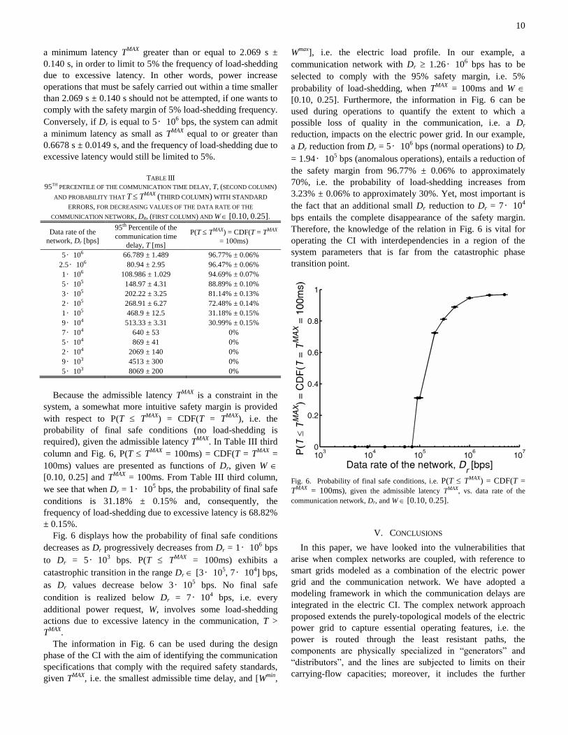
Because the admissible latency TMAX

is a constraint in the

system, a somewhat more intuitive safety margin is provided

with respect to P(T TMAX

) = CDF(T = TMAX

), i.e. the

probability of final safe conditions (no load-shedding is

required), given the admissible latency TMAX

. In Table III third

column and Fig. 6, P(T TMAX

= 100ms) = CDF(T = TMAX

=

100ms) values are presented as functions of Dr, given W

[0.10, 0.25] and TMAX

= 100ms. From Table III third column,

we see that when Dr = 1‧ 105 bps, the probability of final safe

conditions is 31.18% ± 0.15% and, consequently, the

frequency of load-shedding due to excessive latency is 68.82%

± 0.15%.

Fig. 6 displays how the probability of final safe conditions

decreases as Dr progressively decreases from Dr = 1‧ 106 bps

to Dr = 5‧ 103 bps. P(T T

MAX = 100ms) exhibits a

catastrophic transition in the range Dr [3‧ 105, 7‧ 10

4] bps,

as Dr values decrease below 3‧ 105 bps. No final safe

condition is realized below Dr = 7‧ 104 bps, i.e. every

additional power request, W, involves some load-shedding

actions due to excessive latency in the communication, T >

TMAX

.

The information in Fig. 6 can be used during the design

phase of the CI with the aim of identifying the communication

specifications that comply with the required safety standards,

given TMAX

, i.e. the smallest admissible time delay, and [Wmin

,

Wmax

], i.e. the electric load profile. In our example, a

communication network with Dr 1.26‧ 106 bps has to be

selected to comply with the 95% safety margin, i.e. 5%

probability of load-shedding, when TMAX

= 100ms and W

[0.10, 0.25]. Furthermore, the information in Fig. 6 can be

used during operations to quantify the extent to which a

possible loss of quality in the communication, i.e. a Dr

reduction, impacts on the electric power grid. In our example,

a Dr reduction from Dr = 5‧ 106 bps (normal operations) to Dr

= 1.94‧ 105 bps (anomalous operations), entails a reduction of

the safety margin from 96.77% ± 0.06% to approximately

70%, i.e. the probability of load-shedding increases from

3.23% ± 0.06% to approximately 30%. Yet, most important is

the fact that an additional small Dr reduction to Dr = 7‧ 104

bps entails the complete disappearance of the safety margin.

Therefore, the knowledge of the relation in Fig. 6 is vital for

operating the CI with interdependencies in a region of the

system parameters that is far from the catastrophic phase

transition point.

Fig. 6. Probability of final safe conditions, i.e. P(T TMAX) = CDF(T =

TMAX = 100ms), given the admissible latency TMAX, vs. data rate of the

communication network, Dr, and W [0.10, 0.25].

V. CONCLUSIONS

In this paper, we have looked into the vulnerabilities that

arise when complex networks are coupled, with reference to

smart grids modeled as a combination of the electric power

grid and the communication network. We have adopted a

modeling framework in which the communication delays are

integrated in the electric CI. The complex network approach

proposed extends the purely-topological models of the electric

power grid to capture essential operating features, i.e. the

power is routed through the least resistant paths, the

components are physically specialized in “generators” and

“distributors”, and the lines are subjected to limits on their

carrying-flow capacities; moreover, it includes the further

11

complexity that arises from the variability of power generation

from renewable energy sources and intermittent load

consumption. However, given the somewhat abstract level of

the modeling supporting complex network analysis, the

insights gained with respect to the vulnerable areas in the

system (first findings) may not be clear-cut, and major hidden

vulnerabilities may still be expected. Then, to accurately

model the physical behavior of the interconnected systems,

computational frameworks that propagate the flows of power

and information based on physical laws have to be embraced,

and more detailed information about the system and its

operating environment may be needed. For large, real-scale

systems, this requires the development of adequate

computational methodologies through clustering computing,

co-operative simulation, or similar architectures [44]-[48].

We have quantified the limitations that both the electric

power grid and the communication network impose on the

operations of the CI with interdependencies, when a load bus

demands additional power from the generators. In the

application to the 380 kV Italian power transmission network,

with the assumptions made and the numerical data used, we

have observed that a factual indicator for quantifying the

coupling strength between the two integrated systems is the

frequency of load-shedding actions due to excessive

communication time delay. By means of this indicator, we

have evaluated the extent to which a loss of quality in the

communication impacts on the electric power grid, and we

have selected appropriate communication specifications, i.e.

the data rate of the network, that comply with the required

safety requirements in the electric power grid.

Finally, we have detected a catastrophic phase transition

point in the frequency of faulty conditions with respect to the

data rate of the communication network. The CI with

interdependencies safely operate only in a region of the system

parameters that are far from this catastrophic transition point.

To this aim, the introduction of adequate safety margins with

respect to the data rate of the communication network is

suggested.

In summary, the main contributions to the knowledge

generated for the network general case are: (i) the extension of

the purely-topological complex network modeling framework

by inclusion of relevant physical aspects of the system; (ii) the

use of the frequency of load-shedding actions due to excessive

communication time delay as a quantitative indicator for

quantifying the vulnerability of the smart grid; (iii) the

detection of a catastrophic phase transition with respect to the

data rate of the communication network in the smart grid.

[APPENDIX]

[Appendix was removed because it was related to the results

of Section IV.A which were also removed.]

ACKNOWLEDGMENT

The authors are very thankful to the four anonymous

reviewers for helping in improving the paper through their

observations and suggestions.

REFERENCES

[1] W. Kröger and E. Zio, Vulnerable Systems. London, UK: Springer

London, 2011.

[2] S. M. Rinaldi, “Modeling and simulating critical infrastructures and

their interdependencies,” in Proc. Thirty-Seventh Annu. Hawaii Int.

Conf. Syst. Sci., Jan. 5-8, 2004, Waikoloa, Big Island, Hawaii,

Computer Society Press, 2004.

[3] R. Zimmerman, “Social implications of infrastructure network

interactions,” J. Urban Technol., vol. 8, no. 3, pp. 97–119, Dec. 2001.

[4] J. Heckel, “Smart Substation and Feeder Automation for a SMART

Distribution Grid,” in Proc. CIRED 2009 - 20th Int. Conf. and

Exhibition on Electr. Distrib. - Part 1, Jun. 8-11, 2009, London, UK:

The Institution of Engineering and Technology, 2009.

[5] M. Granger Morgan, J. Apt, L. B. Lave, M. D. Ilic, M. Sirbu, and J. M.

Peha, The many meanings of "Smart Grid". A Briefing Note from the

Department of Engineering and Public Policy, Carnegie Mellon

University, Jul. 2009 – url: http://repository.cmu.edu/epp/22/

[6] Smart Grid Laboratory - Energylab, Smart Grid. Le reti elettriche di

domani. Milano, Italy: Gruppo Italia Energia (Gieedizioni), 2011 (in

Italian).

[7] V. K. Sood, D. Fischer, J. M. Eklund, and T. Brown, “Developing a

communication infrastructure for the Smart Grid,” in Proc. IEEE Electr.

Power Energy Conf. (EPEC), Oct. 22 - 23, Montréal, Canada, IEEE,

2009.

[8] M. D. Ilić, L. Xie, U. A. Khan, and J. M. F. Moura, “Modeling of Future

Cyber–Physical Energy Systems for Distributed Sensing and Control,”

IEEE Trans. Syst., Man, Cybern. A, Syst., Humans, vol. 40, no. 4, pp.

825–838, Jul. 2010.

[9] A. Ababnah and B. Natarajan, “Optimal Control-Based Strategy for

Sensor Deployment,” IEEE Trans. Syst., Man, Cybern. A, Syst.,

Humans, vol. 41, no. 1, pp. 97–104, Jan. 2011.

[10] S. Conti and S. Raiti, “Probabilistic load flow using Monte Carlo

techniques for distribution networks with photovoltaic generators,” Sol.

Energy, vol. 81, no. 12, pp. 1473-1481, Dec. 2007.

[11] M. H. Albadi and E. F. El-Saadany, “Overview of wind power

intermittency impacts on power systems,” Electr. Power Syst. Res., vol.

80, no. 6, pp. 627–632, Jun. 2010.

[12] Y. Wang and L. Li, “Effects of Uncertainty in Both Component

Reliability and Load Demand on Multistate System Reliability,” IEEE

Trans. Syst., Man, Cybern. A, Syst., Humans, to be published.

[13] F. Zanellini, Rete e vento – Lo sviluppo della rete elettrica italiana per

la connessione e l’integrazione della fonte eolica. Milano, Italy: Centro

Studi APER – REEF Onlus, May 2011 (in Italian).

[14] The Advisory Council of ‘SmartGrids’ – European Technology Platform

for the Electricity Network of the Future, “Strategic Deployment

Document for Europe’s Electricity Networks of the Future,” Apr. 2010

– url: http://www.smartgrids.eu/documents/SmartGrids_SDD_FINAL_

APRIL2010.pdf

[15] S. Galli, A. Scaglione, and Z. Wang, “For the Grid and Through the

Grid: The Role of Power Line Communications in the Smart Grid,”

Proc. IEEE, vol. 99, no. 6, pp. 998-1027, Jun. 2011.

[16] S. W. Lai, G. G. Messier, H. Zareipour, and C. H. Wai, “Wireless

network performance for residential demand-side participation,” in

Proc. IEEE PES Conf. Innovative Smart Grid Technol. Eur. (ISGT

Europe), October 11-13, 2010, Gothenburg, Sweden, IEEE Power and

Energy Society, 2010.

[17] C.-W. Ten, G. Manimaran, and C.-C. Liu, “Cybersecurity for Critical

Infrastructures: Attack and Defense Modeling,” IEEE Trans. Syst., Man,

Cybern. A, Syst., Humans, vol. 40, no. 4, pp. 853–865, Jul. 2010.

[18] C. Peng, Y.-C. Tian, and D. Yue, “Output Feedback Control of

Discrete-Time Systems in Networked Environments,” IEEE Trans.

Syst., Man, Cybern. A, Syst., Humans, vol. 41, no. 1, pp. 185–190, Jan.

2011.

[19] I. Dobson, B. A. Carreras, and D. E. Newman, “A loading-dependent

model of probabilistic cascading failure,” Probab. Eng. Inf. Sci., vol.

19, no. 1, pp. 15-32, 2005.

[20] H. Hines and S. Blumsack, “A Centrality Measure for Electrical

Networks,” in Proc. 41st Annu. Hawaii Int. Conf. Syst. Sci., Jan. 7-10,

2008, Waikoloa, Big Island, Hawaii, Computer Society Press, 2008.

12

[21] P. Holme, “Edge overload breakdown in evolving networks,” Phys. Rev.

E, vol. 66, no. 3, pp. 036119, 2002.

[22] P. Kinney, P. Crucitti, R. Albert, and V. Latora, “Modeling cascading

failures in the North American power grid,” Eur. Phys. J. B, vol. 46, no.

1, pp. 101-107, 2005.

[23] A. E. Motter and Y.-C. Lai, “Cascade-based attacks on complex

networks,” Phys. Rev. E, vol. 66, no. 6, pp. 065102(R), 2002.

[24] J. Wu, M. Barahona, Y.-J. Tan, and H.-Z. Deng, “Spectral Measure of

Structural Robustness in Complex Networks,” IEEE Trans. Syst., Man,

Cybern. A, Syst., Humans, vol. 41, no. 6, pp. 1244–1252, Nov. 2011.

[25] W.-C. Yeh, “An Improved Method for Multistate Flow Network

Reliability With Unreliable Nodes and a Budget Constraint Based on

Path Set,” IEEE Trans. Syst., Man, Cybern. A, Syst., Humans, vol. 41,

no. 2, pp. 350–355, Mar. 2011.

[26] M. G. Kallitsis, G. Michailidis, and M. Devetsikiotis, “A Framework for

Optimizing Measurement-Based Power Distribution under

Communication Network Constraints,” in Proc. First IEEE Int. Conf.

Smart Grid Commun. (SmartGridComm), Gaithersburg, Maryland,

USA, 4-6 Oct. 2010, Institute of Electrical and Electronic Engineers,

2010.

[27] J. W. Stahlhut, T. J. Browne, G. T. Heydt, and V. Vittal, “Latency

Viewed as a Stochastic Process and its Impact on Wide Area Power

System Control Signals,” IEEE Trans. Power Syst., vol. 23, no. 1, pp.

84-91, 2008.

[28] L. Kleinrock, Queuing g systems. New York, USA: John Wiley & Sons,

Inc., 1975.

[29] Terna S.p.A. - Rete Elettrica Nazionale, Dati statistici sull’energia

elettrica in Italia, 2002. (in Italian) – url:

http://www.terna.it/LinkClick.aspx?fileticket=PUvAU57MlBY%3d&ta

bid=41 8&mid=2501

[30] V. Rosato, S. Bologna, and F. Tiriticco, “Topological properties of high-

voltage electrical transmission networks,” Electr. Power Syst. Res., vol.

77, no. 2, pp. 99-105, 2007.

[31] G. F. White, Natural hazards: local, national and global. New York,

NY: Oxford University Press, 1974, p. 288.

[32] S. Bouchon, “The vulnerability of interdependent critical infrastructures

systems: epistemological and conceptual state-of-the-art,” EU

Commission, Joint Research Centre, Ispra, Italy, EU Report, 2006.

[33] A. M. Cramer, S. D. Sudhoff, and E. L. Zivi, “Metric Optimization-

Based Design of Systems Subject to Hostile Disruptions,” IEEE Trans.

Syst., Man, Cybern. A, Syst., Humans, vol. 41, no. 5, pp. 989–1000,

Sep. 2011.

[34] J. Johansson and H. Hassel, “An approach for modelling interdependent

infrastructures in the context of vulnerability analysis,” Rel. Eng. Syst.

Safety, vol. 95, no. 12, pp. 1335–1344, Dec. 2010.

[35] E. Camponogara, D. Jia, B. H. Krogh, and S. Talukdar, “Distributed

model predictive control,” IEEE Control Syst. Mag., vol. 22, no. 1, pp.

44-52, 2002.

[36] A. Tizghadam and A. Leon-Garcia, “Betweenness Centrality and

Resistance Distance in Communication Networks,” IEEE Netw., vol.

24, no. 6, pp. 10-16, 2010.

[37] J. Irvine and D. Harle, Data Communications and Networks. West

Sussex, UK: Wiley, 2001.

[38] R. M. Metcalfe, Packet Communication. San Jose, CA: Peer-to-peer

Communications, 1996.

[39] J. Daigle, Queuing Theory with Applications to Packet

Telecommunication. New York, USA: Springer Science, 2005.

[40] K. Hopkinson, X. Wang, R. Giovanini, J. Thorp, K. Birman, and D.

Coury, “EPOCHS: A platform for agent-based electric power and

communication simulation built from commercial off-the-shelf

components,” IEEE Trans. Power Syst., vol. 21, no. 2, pp.548-558,

2006.

[41] F.-L. Lian, J. R. Moyne, and D. M. Tilbury, “Performance evaluation of

control networks: Ethernet, ControlNet, and DeviceNet,” IEEE Control

Syst. Mag., vol. 21, no. 1, pp. 66-83, 2001.

[42] D. Gross and C. M. Harris, Fundamentals of Queuing Theory. New

York, NY: Wiley, 1998.

[43] W. T. Song and B. W. Schmeiser, “Omitting Meaningless Digits in

Point Estimates: The Probability Guarantee of Leading-Digit Rules,”

Oper. Res., vol. 57, no. 1, pp. 109–111, 2009.

[44] Advances in Computers - Parallel, Distributed, and Pervasive

Computing, A. R. Hurson and M. V. Zelkovits eds., vol. 63, San Diego,

Ca, USA: ELSEVIER Inc., 2005.

[45] M. Verhoef, P. Visser J. Hooman, and J. Broenink, “Co-simulation of

Distributed Embedded Real-Time Control Systems,” in Proc. 6th Int.

Conf. Integr. Formal Methods, IFM 2007, Oxford, UK, July 2-5, 2007,

J. Davies and J. Gibbons (Eds.), Berlin, Germany: Springer-Verlag,

2007.

[46] C. Jiang, X. Xu, and J. Wan, “Grid Computing Based Large Scale

Distributed Cooperative Virtual Environment Simulation,” in Proc. 12th

Int. Conf. Comput. Supported Cooperative Work in Design, Xi'an,

Cina, 16-18 April 2008, Piscataway, NJ, USA: IEEE Press, 2008.

[47] T. Tomura, S. Kanai, and T. Kishinami, “A Cooperative Simulation

Mechanism of Distributed Control Systems based on Object-Oriented

Design Patterns,” in Proc. 6th IEEE Int. Symposium on Object-Oriented

Real-Time Distrib. Comput., Hakodate, Hokkaido, Japan, 14-16 May

2003, Piscataway, NJ, USA: IEEE Press, 2003.

[48] P. A.F. Ferreira, E. F. Esteves, R. J.F. Rossetti, and E. C. Oliveira, “A

Cooperative Simulation Framework for Traffic and Transportation

Engineering,” in Proc. 5th Int. Conf. Cooperative Design, Visual., Eng.,

Calvià, Mallorca, Spain, September 21-25, 2008, Berlin, Germany:

Springer-Verlag, 2008.

Enrico Zio (BS in nuclear engng., Politecnico di

Milano, 1991; MSc in mechanical engng., UCLA,

1995; PhD, in nuclear engng., Politecnico di

Milano, 1995; PhD, in nuclear engng., MIT, 1998)

is Director of the Chair in Complex Systems and

the Energetic Challenge of the European

Foundation for New Energy of Electricite’ de

France (EDF) at Ecole Centrale Paris and Supelec,

full professor, President and Rector's delegate of

the Alumni Association and past-Director of the

Graduate School at Politecnico di Milano, adjunct

professor at University of Stavanger. He is the Chairman of the European

Safety and Reliability Association ESRA, member of the scientific committee

of the Accidental Risks Department of the French National Institute for

Industrial Environment and Risks, member of the Korean Nuclear society and

China Prognostics and Health Management society, and past-Chairman of the

Italian Chapter of the IEEE Reliability Society. He is serving as Associate

Editor of IEEE Transactions on Reliability and as editorial board member in

various international scientific journals, among which Reliability Engineering

and System Safety, Journal of Risk and Reliability, International Journal of

Performability Engineering, Environment, Systems and Engineering,

International Journal of Computational Intelligence Systems. He has

functioned as Scientific Chairman of three International Conferences and as

Associate General Chairman of two others. His research focuses on the

characterization and modeling of the failure/repair/maintenance behavior of

components, complex systems and critical infrastructures for the study of

their reliability, availability, maintainability, prognostics, safety, vulnerability

and security, mostly using a computational approach based on advanced

Monte Carlo simulation methods, soft computing techniques and

optimization heuristics. He is author or co-author of five international books

and more than 170 papers on international journals.

Giovanni Sansavini (B.S. in energy engineering,

Politecnico di Milano, 2003; M.Sc. in nuclear

engineering, Politecnico di Milano, 2005; Ph.D.,

in nuclear engineering, Politecnico di Milano,

2010; Ph.D., in engineering mechanics, Virginia

Tech, 2010) is a Postdoctoral Research Assistant

at the Department of Energy, Politecnico di

Milano. His research interest is the analysis of the

reliability, safety, and security of complex systems

under stationary and dynamic operation.