Embed Size (px)
Citation preview

UNIVERSITE DE PARIS IX-DAUPHINE
U.F.R. MATHEMATIQUES DE LA DECISION
N attribue par la bibliotheque
THESE
pour obtenir le grade de
DOCTEUR EN SCICECES DE L’UNIVERSITE PARIS IX
SPECIALITE MATHEMATIQUES APPLIQUEES
presentee et soutenue publiquement par
VU Thanh Nam
le 17 Octobre 2011
Titre:
Controle Stochastique Applique a la Finance
Directeur de these: Bruno Bouchard-Denize
JuryM. Pham Huyen, Rapporteur
M. Halil Mete Soner, Rapporteur
M. Peter Tankov, Examinateur
M. Romauld Elie, Examinateur
M. Bruno Bouchard-Denize, Directeur de these

2

Abstract
This PhD dissertation presents three independent research topics in the field
of stochastic target and optimal control problems with applications to financial
mathematics.
In a first part, we provide a PDE characterization of the super hedging price of
an American option of barrier types in a Markovian model of financial market. This
extends to the American case a recent works of Bouchard and Bentahar [9], who
considered European barrier options, and Karatzas and Wang [29], who discussed
the case of perpetual American barrier options in a Black and Scholes type model.
Contrary to [9], we do not use the usual dual formulation, which allows to reduce to
a standard control problem, but instead prove and appeal to an American version
of the geometric dynamic programming principle for stochastic targets of Soner and
Touzi [47]. This allows us to avoid the non-degeneracy assumption on the volatility
coefficients of [9], and therefore extends their results to possibly degenerate cases
which typically appear when the market is not complete. As a by-product, we provide
an extension to the case of American type targets of the result of [47], which is of
own interest.
In the second part, within a Brownian diffusion Markovian framework, we pro-
vide a direct PDE characterization of the minimal initial endowment required so
that the terminal wealth of a financial agent (possibly diminished by the payoff
of a random claim) can match a set of constraints in probability. Such constraints
should be interpreted as a rough description of a targeted profit and loss (P&L)
distribution. This allows to give a price to options under a P&L constraint, or to
provide a description of the discrete P&L profiles that can be achieved given an
initial capital. This approach provides an alternative to the standard utility indiffe-
rence (or marginal) pricing rules which is better adapted to market practices. From
the mathematical point of view, this is an extension of the stochastic target pro-
blem under controlled loss, studied in Bouchard, Elie and Touzi [12], to the case of
multiple constraints. Although the associated Hamilton-Jacobi-Bellman operator is
fully discontinuous, and the terminal condition is irregular, we are able to construct
a numerical scheme that converges at any continuity points of the pricing function.
The last part of this thesis is concerned with the extension of the optimal control
3

ABSTRACT
of direction of reflection problem introduced in Bouchard [8] to the jump diffusion
case. In a Brownian diffusion framework with jumps, the controlled process is defined
as the solution of a stochastic differential equation reflected at the boundary of a
domain along oblique directions of reflection which are controlled by a predictable
process which may have jumps. We also provide a version of the weak dynamic
programming principle of Bouchard and Touzi [14] adapted to our context and which
is sufficient to provide a viscosity characterization of the associated value function
without requiring the usual heavy measurable selection arguments nor the a-priori
continuity of the value function.
4

Introduction generale
Dans la litterature, un probleme de cible stochastique est souvent etudie en
utilisant des arguments de dualite qui permet de se ramener a un probleme ecrit
sous une forme standard de controle stochastique, voir par exemple Cvitanic et
Karatzas [19], Follmer et Kramkov [22], et, Karatzas et Shreve [30]. Cependant,
cette approche ne requiert pas seulement la preuve d’une formulation duale, mais
aussi ne s’appliquent qu’aux dynamiques lineaires. Afin d’eviter ces difficultes, on
se base sur les etapes introduites par Soner et Touzi [46] et [47], qui ont propose un
nouveau principe de la programmation dynamique, appele geometrique. Cela ouvre
les portes pour un nombre vaste d’applications, notamment pour le controle des
risques en finance et assurance. Dans un cadre markovien, il permet de deriver les
equations aux derivees partielles associees au probleme de cible stochastique de la
maniere plus directe, a l’exception de la formulation standard de dualite, voir [51]
et [44].
L’objectif principal de cette these est d’etendre leurs resultats a des applica-
tions importantes dans le controle des risques en finance et en assurance. En par-
ticulier, nous proposons une extension du principe de la programmation dyna-
mique geometrique, qui est associee a une option barriere de type americain avec
contraintes. Nous etudions egalement une classe de problemes de cible stochastique
avec multiples contraintes au sens de la probabilite. Ceci caracterise le prix de sur-
replication sur une forme de P&L comme une unique solution de viscosite d’une
equation aux derivees partielles. Finalement, nous considerons une version faible du
principe classique de la programmation dynamique introduite par Bouchard et Touzi
[14] et l’appliquons a une nouvelle classe de problemes de controle stochastique as-
sociees a des diffusions mixtes. En laquelle le processus controle est defini comme la
solution d’une equation differentielle stochastique, qui est rejetee a la frontiere d’un
domaine borne O et ses directions de reflexion peuvent etre controlees. Cette these
est organisee selon les trois parties suivant.
Dans la premiere partie, notre objectif est de caracteriser les options barrieres
des type americain dans un modele markovien du marche financier a l’aide des
solutions de viscosite. Recemment, ce probleme a ete etudie par Bouchard et Ben-
tahar [9] qui ont considere la couverture sous contraintes avec une barriere dans un
5

INTRODUCTION GENERALE
contexte europeen, ainsi qu’une extension du resultat precedent de Shreve, Schmock
et Wystup [41]. Karatzas et Wang [29] ont traite de une facon similaire pour les
options barrieres de type americain dans un modele de Black-Scholes. La difficulte
principale provient de la condition au bord ∂O avant une maturite. Au cas d’option
vanille, il faut envisager une version ’face-lifted’ du pay-off comme une condition au
bord. Cependant, cette condition est insuffisante pour traiter une option barriere
plus generale et doit etre consideree au sens faible, voir [41]. Ceci conduit a une
melange de la condition au bord de type Neumann et Dirichlet. Au cas americain,
un phenomene similaire apparait, mais nous devons egalemnt faire attention au fait
que l’option peut etre exercee a tout moment avant une maturite.
Au contraire de Bouchard et Bentahar [9], nous n’utilisons pas le formulation
usuelle de dualite, au lieu d’appliquer le principe de la programmation dynamique
geometrique (PPDG) au probleme de cible stochastique. On commence par etendre
le travail de Soner et Touzi [47] sur une cible de type americain, applee une version
’obstacle’. En general, un probleme de cible americaine stochastique est introduit
suivant : trouver l’ensemble V (0) des conditions initiales z pour Zν0,z tel que Z
ν0,z(t) ∈
G(t) ∀ t ∈ [0, T ] P−a.s. pour un controle ν. Ici, t 7→ G(t) est une fonction en prenant
des valeurs dans la collection de sous-ensembles borelienne de Rd. Dans le Chapitre
1, nous proposons une version obstacle du PPDG ecrit sous la forme :
V (t) = z ∈ Rd : ∃ ν ∈ A s.t Zνt,z(τ ∧ θ) ∈ G
τ,θ⊕V P− p.p ∀ τ ∈ T[t,T ], (0.1)
ou
G
τ,θ⊕V := G(τ) 1τ≤θ + V (θ) 1τ>θ
et T[t,T ] designant l’ensemble des temps d’arret a valeurs dans [t, T ]. Nous concluons
cette partie a traiter l’application de la version obstacle au-dessus a l’option barriere
americaine avec contraintes dans le Chaptre 2. Soitent un modele markovien du
marche financier compose d’un actif non risque et d’une ensemble des d actifs risques
X = (X1, ..., Xd), et un processus de la richesse Y πt,x,y associee a un capital initial
y ∈ R+ et une strategie financiere π. Une option barriere de type americaine est
exprime par une fonction g definie sur [0, T ] × Rd+ et par un domaine ouvert O of
Rd+ pour que l’acheteur recoive le paiement g(θ,Xt,x(θ)) quand il exerce l’option
au moment de θ ≤ τt,x, ou τt,x est le temps de la premiere sortie du processus de
prix Xt,x en dehors d’un domaine ouvert O. Dans ce cas, l’ensemble des dotations
associees a notre probleme est donne par
V (t, x) := y ≥ R+ : ∃ π t.q. Zπt,x,y(τ ∧ τt,x) ∈ G(τ ∧ τt,x) ∀ τ ∈ T[t,T ],
avec Zπt,x,y := (Xt,x, Y
πt,x,y) et G(t) := (x, y) ∈ O × R+ : y ≥ g(t, x). Ensuite,
la fonction valeur v(t, x) := inf V (t, x) caracterise completement l’inferieur de l’en-
semble V (t, x) et une version du PPDG peut etre declaree en termes de la fonction
6

INTRODUCTION GENERALE
valeur v :
(DP1) Si y > v(t, x), alors il existe une strategie financiere π telle que
Y πt,x,y(θ) ≥ v(θ,Xt,x(θ)) pour tout θ ∈ Tt,x .
(DP2) Si y < v(t, x), alors il existe τ ∈ Tt,x tel que
P[Y πt,x,y(θ ∧ τ) > v(θ,Xt,x,y(θ))1θ<τ + g(τ,Xt,x,y(τ))1θ≥τ
]< 1
pour toute strategie financiere π and θ ∈ Tt,x := τ ∈ T[t,T ] : τ ≤ τt,x.L’analyse ci-dessus peut etre comparee a Soner et Touzi [49], auquel l’auteurs ont
considere une option de type europeen. Et la preuve est vraiment tres proches lorsque
la programmation dynamique (DP2) est remplacee par une forme correspondante.
Les differences principales proviennent du fait que nous n’imposons pas l’hypothese
de non-degenerescence sur les coefficients des actifs financiers sous-jacents. Cette hy-
pothese apparaissent dans les marches financiers complets et est aussi necessaire a
la formulation de dualite, voir [9], [13], [19], [28] et [29]. Nous prenons cette occasion
pour expliquer comment ce probeme peut etre traite et etre transpose a l’option
americaine sans barriere dont nous parlerons plus tard a la fin de ce chapitre. Afin
de separer les difficultes, on se restreint au cas ou les strategies de π sont a valeurs
dans un ensemble compact convexe donne. Le cas du controle non borne peut etre
manipule a l’aide de la technique developpee par Bouchard , Elie et Touzi [12]. De
meme, les sauts pourrait etre ajoutee a la dynamique sans aucunes difficultes ma-
jeures, voir Bouchard [7].
Dans la deuxieme partie, nous etudions la plus petite richesse initiale telle
que la richesse terminale d’un agent financier peut etre satisfaite d’un ensemble
de contraintes en probabilite. En pratique, cet ensemble de contraintes doit etre
considere comme une description sommaire d’une distribution ciblee de P&L. Plus
precisement, nous supposons que la valeur liquidative de l’option s’ecrit g(Xt,x(T )),
ou Xt,x sont les actifs risques. Le processus de la richesse Y νt,x,y est associe a partir de
un capital initial y ∈ R+ et une strategie financiere ν. Pour une collection des seuils
γ := (γi)i≤κ ∈ Rκ et des probabilites p := (pi)i≤κ ∈ [0, 1]κ, le prix de l’option est
defini comme le plus petit capital initial y tel que il existe une strategie financiere
π pour quelle le filet de la perte ne depasse pas −γi avec une probabilite plus de
pi pour tout i ∈ 1, . . . , κ. Cela conduit a une contrainte pour la distribution de
P&L qui est imposee par un histogramme discret associe a (γ, p). En evitant la
grande negativite du processus de richesse ( meme avec une probabilite faible), nous
egalement imposons que Y νt,x,y(T ) ≥ ℓ pour certains ℓ ∈ R−. Le prix est alors ecrit
7

INTRODUCTION GENERALE
sous la forme suivante :
v(t, x, p) := (0.2)
infy : ∃ ν s.t. Y νt,x,y(T ) ≥ ℓ, P
[Y νt,x,y(T )− g(Xt,x(T )) ≥ −γi
]≥ pi ∀ i ≤ κ,
ou on supppose que γκ ≥ · · · ≥ γ2 ≥ γ1 ≥ 0.
Car γi ≥ γj pour i ≤ j, notre probleme naturellement se limite aux cas pi ≤ pj
pour i ≤ j. Ceci conduit a l’introduction de conditions aux bords sur les plans ou
pi = pj pour certains i 6= j. Mais cette restriction n’est pas ncessaire dans notre
approche. Nous alors ne l’utilisons pas et nous concentrons sur les points de la
frontiere (t, x, p) tels que pi = 0 ou pi = 1. Du point de vue numerique, on pourrait
cependant utiliser le fait que v(·, p) = v(·, p), ou p est defini par pj = maxi≤j pj pour
i ≤ κ.
Au cas κ = 1, un tel probleme est appele le “quantile hedging problem”. Il a
ete largement etudie par Follmer and Leukert [23] qui ont donne une description
explicite de la richesse terminale optimale de Y νt,x,y(T ) quand le sous-jacente du
marche financier est complet. Ce resultat est derive d’une utilisation intelligente du
Lemme de Neyman-Pearson en statistiques mathematiques et s’applique aux cadres
non-Markoviens. Ensuite, une approche directe, basee sur la notion de problemes
cibles stochastiques, a ete proposee par Bouchard, Elie et Touzi [12]. Cela nous
permet de caracteriser la fonction valeur meme dans les marches incomplets ou dans
les cas ou le processus de prix Xt,x peut etre influence par la strategie de negociation
ν, voir par exemple Bouchard et Dang [10]. Le probleme (0.2) est une generalisation
de ce travail au cas de multiples contraintes en probabilite.
Comme dans [12], la premiere etape consiste a recrire (0.2) comme un probleme
standard de cible stochastique :
v(t, x, p)
= infy : ∃ (ν, α) t.q Y νt,x,y(T ) ≥ ℓ,min
i≤κ
(1Y ν
t,x,y(T )−g(Xt,x(T ))≥−γi − P α,it,p (T )
)≥ 0 .
La reduction ci-dessus est obtenu par ajouter une famille de martingales bornees d-
dimensionnelles P αt,p dont i-eme composante P α,i
t,p est definie par la representation des
martingales pour 1Y νt,x,y(T )−g(Xt,x(T ))≥−γi. Il conduit a un principe de la program-
mation dynamique geometrique, qui nous permet de caracteriser la fonction valeur
comme une solution discontinue de viscosite d’une certaine equation aux derivees
partielles. Dans cette these, on etudie des telles equations dans le cadre de marches
complets pour deux cas suivants.
Au premier cas, le montant d’argent investi dans les actifs risques est nonborne,
voir l’exemple d’une option d’achat dans le modele de Black-Scholes dans Follmer
and Leukert [23]. Un operateur associe de Hamilton-Jacobi-Bellman est indique dans
8

INTRODUCTION GENERALE
la Subsection 4 du Chapitre 3 avec une condition terminale :
v∗(T, x, p) = v∗(T, x, p) = l(1−maxi≤κ
pi) +
κ−1∑
i=0
(g(x)− γi+1)(pi+1 −maxk≤i
pk)+. (0.3)
Nous nous concentrons sur le deuxieme cas ou le montant d’argent investi dans
les actifs risques est borne. C’est a dire que les strategies financieres ν appartient
a l’ensemble U de processus progressivement mesurable prenant des valeurs dans
un sous-ensemble compact U de Rd. Dans ce cas, la condition terminale de v n’est
pas une forme naturelle de (0.3) a cause de l’absence de convexite par rapport a
la variable p. De plus, l’apparition de la contrainte de gradient ”diag [x]Dxv ∈ U”
conduit a la version ”facelifted ” de g, applee g, voir par exemple Cvitanic, Pham
et Touzi [20]. En suite, la condition terminale peut etre naturellement formulee au
termes faible v∗(T, ·) ≥ G∗ and v∗(T, ·) ≤ G∗, ou
G(x, p) := maxi∈K
(ℓ1pi=0 + (g(x)− γi)10<pi<1 + (g(x)− γi)1pi=1
).
Il est clair que G∗ < G∗ pour certain p ∈ ∂[0, 1]κ et l’operateur associe de Hamilton-
Jacobi-Bellman is egalement discontinu. Ceci est impossible d’etablir un resultat
de comparaison et aussi de construire un schema numerique base sur ce operateur.
Afin de resoudre ces difficultes, nous introduisons dans le Chapitre 4 une sequence
de problemes approximatifs qui sont plus reguliers et pour lesquels une convergence
des schemas numerique associes est obtenue. En particulier, nous montrerons que
une telle sequence permet de preciser une estimation de les problemes suivantes :
v(t, x, p) = inf
y : ∀ε > 0 ∃νε t.q. Y νε
t,x,y(T ) ≥ ℓ,
P[Y νε
t,x,y(T )− g(Xt,x(T )) ≥ −γi]≥ pi − ε ∀ i
et
v(t, x, p)
= infy : ∃ ν t.q. Y νt,x,y(T ) ≥ ℓ , P
[Y νt,x,y(T )− g(Xt,x(T )) ≥ −γi
]> pi ∀ i ≤ κ.
On montre effectivement que la premiere fonction value v est la limite a gauche
en p de v tandis que la deuxieme v est la limite a droid en p de v. Aux cas ou v
is continu, en suite v = v = v et nos schemas convergent vers la fonction valeur
originale. Cependant, il semble que cette continuite est difficultee de etre demontree
par les absences de la convexite et de la monotonie stricte de la fonction indicatrice.
Pourtant, l’un des deux approximations ci-dessus peut etre choisi pour resoudre des
problemes pratiques.
Dans la derniere partie, nous considerons un probleme de controle optimal
stochastique pour les processus de reflexion dans un cadre de la diffusion Brownienne
9

INTRODUCTION GENERALE
avec des sauts. L’originalite de ce travail provient du fait que le processus controle
est defini comme la solution d’une equation differentielle stochastique qui se reflete
a la frontiere d’un domaine O. La direction de reflexion obique γ est controlee par
un processus previsible qui peut avoir des sauts.
Lorsque la direction de reflexion γ n’est pas controlee, on obtient une classe des
equations differentielles stochastiques plus simples avec reflexion, dans lequelle le
processus de reflexion est defini sur R+, voir Skorokhod [42]. Tanaka [50] a montre
l’existence d’une solution de telle equation dans des domaines convexes, voir El
Karoui et Marchan [17], et, Ikeda et Watanabe [26]. Plus tard, Lions et Sznitman
[35] ont etudie le cas ou le domaine O satisfait une condition de la sphere exterieure
uniforme, qui signifie que il existe r > 0 tel que pour tout x ∈ ∂O il y a x1 ∈ Rd
satisfaisant B(x1, r)∩O = x. Etant motive par des applications en mathematiques
financieres, Bouchard [8] ensuite demontree l’existence d’une solution d’une classe
des equations differentielles stochastiques avec la reflexion, dans lesquelle la direction
de reflexion obique est controlee. Ce resultat est limite au cadre de la diffusion
Brownienne et au cas ou le controle est une combinaison d’un processus d’Ito et
d’un processus continu a variation bornee.
Dans le Chaptre 5, nous etendons ces resultats de Bouchard au processus de la
diffusion avec sauts et nous nous permettons d’ajouter des sauts au controle. Au
premiere etape, nous commencons par caracteriser un probleme de Skorokhod :
φ(t) = ψ(t) +
∫ t
0
γ(φ(s), ε(s))1φ(s)∈∂Odη(s), φ(t) ∈ O,
ou η est une fonction non decroissante et γ est controle par un processus de controle
ε a value dans un ensemble compact donne E de Rl. En general, l’existence et
l’unicite des solutions au probleme de Skorokhod avec reflexion oblique reguliere sont
encore des questions ouvertes, seulement quelques cas particuliers ont ete traites. En
particulier, Lions et Sznitman [35] ont montre la telle unicite quand soit le domaineOest regulier, soit il satisfait une condition de la sphere homogene exterieure uniforme
mais le cone de reflexion oblique doit etre transforme en la normale multipliee par une
fonction matricielle reguliere. Quand la direction de reflexion γ n’est pas controlee,
c’est a dire que γ est une fonction reguliere de Rd a Rd qui ne depend pas de ε et
satisfait |γ| = 1, Dupuis et Ishii [21] ont demontre l’existence et l’unicite forte des
solutions pour deux cas. Au premier cas, la direction de reflexion γ a chaque point
de la frontiere est une valeur singuliere et varie doucement, meme si le domaine Opeut etre non regulier, telle que
⋃
0≤λ≤r
B(x− λγ(x), λr) ⊂ Oc, ∀x ∈ ∂O, (0.4)
pour quelque r ∈ (0, 1). Au second cas, on suppose que le domaine O est l’in-
tersection d’un nombre fini de domaines a frontiere reguliere. Dans Bouchard [8],
10
INTRODUCTION GENERALE
l’existence est obtenue lorsque O est un ensemble ouvert borne, γ est une fonction
reguliere de Rd × E a Rd satisfaisant |γ| = 1, et il existe un r ∈ (0, 1) tel que
⋃
0≤λ≤r
B(x− λγ(x, e), λr) ⊂ Oc, ∀(x, e) ∈ ∂O ×E, (0.5)
qui impose uniformement la condition (0.10) dans la variable de controle. Cela per-
met de montrer l’existence forte d’une solution au probleme de Skorokhod dans la
famille de fonctions continues quand ε est une fonction continue a variation bornee.
Nous faison une extension de ce resultat au probleme de Skorokhod pour la famille
des fonctions cadlag ayant un nombre fini de points de discontinuite. La difficulte
vient de la maniere de definir la solution aux temps de sauts. Dans cette these,
nous etudions une classe particuliere de solutions, qui est parametree par le choix
d’un operateur de projection π. Si la valeur de φ(s−) + ∆ψ(s) sors de la cloture
du domaine a un temps de saut, nous projetons cette valeur sur la frontiere ∂Odu domaine selon la direction γ. La valeur apres le saut de φ est choisie egale a
π(φ(s−) + ∆ψ(s), ε(s)), ou la projection π selon la direction oblique γ satisfait
y = π(y, e)− l(y, e)γ(π(y, e), e), pour tous y /∈ O et e ∈ E,
pour une telle fonction positive l. Quand la reflexion n’est pas oblique et le domaine
O est convexe, la fonction π est exactement la projection usuelle et l(y) coincide avec
la distance a la cloture du domaine O. Nous savons deja que l’existence et l’unicite
a un tel probleme entre les temps de saut sont garanties, voir Dupuis et Ishii [21].
Cela conduit a une existence sur l’intervalle de [0, T ], ainsi que les solutions aux
temps de sauts suivent la regle ci-dessus, quand ψ et ε ont seulement un nombre fini
de discontinuites.
Par la suite, nous demontrons l’existence d’une paire unique formee par un pro-
cessus avec reflexion Xε et par un processus non decroissant Lε qui satisfontX(r) = x+
∫ rtF (X(s−))dZs +
∫ rtγ(X(s), ε(s))1X(s)∈∂OdL(s),
X(r) ∈ O, for all r ∈ [t, T ](0.6)
ou Z est la somme d’un drift, une integrale stochastique par rapport au mouvement
Brownien et un processus de Poisson compose, et le processus de controle ε appar-
tient a la classe E de E-valeur processus previsibles cadlag a variation bornee et acti-
vite infinie. Comme le cas deterministe a preciser, nous ne etudions qu’une classe par-
ticuliere de solutions parametree par π. C’est a dire que X est projete sur la frontiere
selon l’operateur de projection π chaque fois qu’il sors du domaine en raison d’un
saut. La valeur apres le saut de X est choisi egal a π(X(s−)+Fs(X(s−))∆Zs, ε(s)).
L’objectif principal du Chapitre 6 est d’etendre le resultat de Bouchard [8] a un
processus de la diffusion avec sauts. Ce processus controle est defini par la solution
de l’equations differentielles stochastiques avec la reflexion (1.2). Nous introduisons
11

INTRODUCTION GENERALE
ensuite un probleme de controle optimal v(t, x) := supε∈E J(t, x; ε), ou la fonction
de cout J(t, x; ε) est definie par
J(t, x; ε) := E
[βεt,x(T )g(X
εt,x(T )) +
∫ T
t
βεt,x(s)f(Xεt,x(s))ds
]
avec βεt,x(s) = e−∫ st ρ(X
εt,x(r−))dLε
t,x(r), l’indice ’t, x’ est la condition initiale de (1.2)
et f, g, ρ sont des fonctions donnees. De facon classique, la technique cle permet-
tante de deriver les equations aux derivees partielles associees est le principe de la
programmation dynamique, voir Bouchard [8], Fleming et Soner [24] et Lions [34].
Bouchard et Touzi [14] ont recemment discute une version faible de celui, qui est
suffisante pour caracteriser la fonction valeur associee au sens de viscosite sans avoir
besoin de l’argument usuel de selection mesurable et de la continuite a priori de la
fonction valeur. Dans ce travail, nous appliquons leur resultat a donner par
v(t, x) ≤ supε∈E
E
[βεt,x(τ)[v
∗, g](τ,Xεt,x(τ)) +
∫ τ
t
βεt,x(s)f(Xεt,x(s))ds
],
et, pour toute fonction semi-continue superieurement ϕ telle que ϕ ≤ v∗,
v(t, x) ≥ supε∈E
E
[βεt,x(τ)[ϕ, g](τ,X
εt,x(τ)) +
∫ τ
t
βεt,x(s)f(Xεt,x(s))ds
],
ou v∗ (resp. v∗) sont l’enveloppe semicontinue superieurement (resp. semi-continue
inferieurement) de v, et [w, g](s, x) := w(s, x)1s<T + g(x)1s=T pour toute fonction
w definee sur [0, T ] × Rd. Cela nous permet de caracteriser la fonction valeur de
v au sens de viscosite. Finalement, nous etendons le principe de comparaison de
Bouchard [8] a notre contexte.
12

Introduction en anglais
In the mathematical finance literature, the problem of super-hedging financial
options has usually been treated via the so-called dual formulation approach, see e.g.
Cvitanic and Karatzas [19], Follmer and Kramkov [22], and, Karatzas and Shreve
[30]. This allows us to convert this problem into a standard stochastic control formu-
lation. However, this not only requires to first prove a suitable duality result but also
essentially only applies to linear dynamics, and is therefore very restrictive. In this
work, we follow the steps of Soner and Touzi [46] and [47], who proposed to appeal
to a new dynamic programming principle, called geometric. Opening the doors to
a wide range of applications, particularly in risk control in finance and insurance,
this provides a direct PDE characterization of super-hedging type problems in very
general Markovian setting, without appealing the standard dual formulation from
mathematical finance, see e.g. [51] and [44].
The main aim of this thesis is to extend their results to some non-trivial applica-
tions in risk control in finance and assurance. In particular, we prove an extension of
the geometric dynamic programming principle, which allows us to study the pricing
of American option under constraints neither with a barrier or without a barrier.
We also study a class of the stochastic target problems with multiple constraints in
probability, which allows to provide a PDE characterization of P&L based option
price in models with constraints on the hedging strategy. Finally, we consider a weak
version of the classical dynamic programming principle introduced in Bouchard and
Touzi [14] and apply it to study a new class of optimal control problem for jumps-
diffusion processes. In which, the controlled process is defined as the solution of a
stochastic differential equation rejected on the boundary of a bounded domain O,
and whose direction of reflection can be controlled. The rest of thesis is organized
as follows.
In the first part of this thesis, our goal is to provide a PDE characterization for
the super hedging price of an American option of barrier types in a Markovian model
of financial market. Recently, this problem has been further studied by Bouchard and
Bentahar [9] who considered the super-hedging under constraints for barrier type
options in a European context, thus extending previous results of Shreve, Schmock
and Wystup [41]. A similar analysis has been carried out by Karatzas and Wang
13

INTRODUCTION EN ANGLAIS
[29] for perpetual American barrier options within a Black and Scholes type finan-
cial model. The main difficulty comes from the boundary condition on ∂O before
maturity. As in the vanilla option case, they have to consider a ’face-lifted’ version
of the pay-off as a boundary condition. However, it turns out not to be sufficient
and this boundary condition has to be considered in a weak sense, see also Shreve,
Schmock and Wystup [41]. This gives a rise to a mixed Neumann/Dirichlet type
boundary condition. In the American case, a similar phenomenon appears but we
also have to take into account the fact that the option may be exercised at any time.
This introduces an additional free boundary feature inside the domain.
In [9], the derivation of the associated PDE relies on the dual formulation of
Cvitanic and Karatzas [19]. Contrary to this, we do not use the usual dual formu-
lation, which allows to reduce to a standard control problem, but instead appeal to
the geometric dynamic programming principle for stochastic targets of Soner and
Touzi [47], call ’an obstacle version’.
In the Chapiter 1, we start with an extension to the case of American type targets
of the result of Soner and Touzi [47], which is of own interest. It can be formalized
as follows. Let us consider a family of d−dimenssional controlled processes Zνt,z with
initial condition Zνt,z = z, depending on a control ν ∈ A. As an obstacle version,
we mean the following problem : find the set V (0) of initial conditions z for Zν0,z
such that Zν0,z(t) ∈ G(t) ∀ t ∈ [0, T ] P−a.s. for some ν ∈ A. Here, t 7→ G(t) is
now a set valued map taking values in the collection of Borel subsets of Rd, which
corresponds to an American target stochastic problem. The main aim of this chapter
is to provide an obstacle version of the geometric dynamic programming principle
to this setting :
V (t) = z ∈ Rd : ∃ ν ∈ A s.t Zνt,z(τ ∧ θ) ∈ G
τ,θ⊕V P− a.s ∀ τ ∈ T[t,T ], (0.7)
where
G
τ,θ⊕V := G(τ) 1τ≤θ + V (θ) 1τ>θ ,
where T[t,T ] denotes the set of stopping times taking values in [t, T ].
The Chapter 2 of this dissertation deals with the application of the above obstacle
version to the super-hedging of an American option of barrier types, in a Markovian
model of financial market. We consider a financial market composed of a non-risky
asset, price process is normalized to unity, and d risky assets X = (X1, ..., Xd).
To an initial capital y ∈ R+ and a financial strategy π, we associate the induced
wealth process Y πt,x,y. The American barrier option is described by a map g defined
on [0, T ]× Rd+ and an open domain O of Rd
+ so that the buyer receives the payoff
g (θ,Xt,x(θ)) when he/she exercises the option at time θ ≤ τt,x, where τt,x is the first
time when Xt,x exits O. In this case, the set of initial endowments that allow one to
14

INTRODUCTION EN ANGLAIS
hedge the claim is given by
V (t, x) := y ≥ R+ : ∃ π s.t. Zπt,x,y(τ ∧ τt,x) ∈ G(τ ∧ τt,x) ∀ τ ∈ T[t,T ],
with Zπt,x,y := (Xt,x, Y
πt,x,y) and G(t) := (x, y) ∈ O × R+ : y ≥ g(t, x).
Then the associated value function v(t, x) := inf V (t, x) completely characterizes
the (interior of the) set V (t, x) and a version of geometric dynamic programming
principle can be stated in terms of the value function v :
(DP1). If y > v(t, x), then there exists a financial strategy π such that
Y πt,x,y(θ) ≥ v(θ,Xt,x(θ)) for all θ ∈ Tt,x .
(DP2) If y < v(t, x), then there exists τ ∈ Tt,x such that
P[Y πt,x,y(θ ∧ τ) > v(θ,Xt,x,y(θ))1θ<τ + g(τ,Xt,x,y(τ))1θ≥τ
]< 1
for all financial strategy π and θ ∈ Tt,x := τ ∈ T[t,T ] : τ ≤ τt,x.The above analysis can be compared to Soner and Touzi [49] who considered
European type options, and the proofs are actually very close once the dynamic
programming (DP2) is replaced by a corresponding one. The main differences come
from the fact that we do not impose a non-degeneracy assumption on the volati-
lity coefficients of the underlying financial assets, which is also required in a dual
formulation, see [9], [13], [19], [28] and [29]. We therefore take this opportunity to
explain how it can be treated, which is of own interest and could be transposed
to the American option without barrier, which we discuss later at the end of this
chapter.
In order to separate the difficulties, we shall restrict to the case where the stra-
tegies π take values in a given convex compact set. The case of unbounded control
sets can be handled by using the technology developed in Bouchard , Elie and Touzi
[12]. Similarly, jumps could be added to the dynamics without major difficulties, see
Bouchard [7].
In the second part, we study a direct PDE characterization of the minimal
initial endowment required so that the terminal wealth of a financial agent (possibly
diminished by the payoff of a random claim) can match a set of constraints in
probability. In practice, this set of constraints has to be viewed as a rough description
of a targeted P&L distribution. To be more precise, let us consider the problem of a
trader who would like to hedge a European claim of the form g(Xt,x(T )), where Xt,x
models the evolution of some risky assets, assuming that their value is x at time
t. Here, the price is chosen so that the net wealth Y νt,x,y(T )− g(Xt,x(T )) satisfies a
P&L constraint. Namely, given a collection of thresholds γ := (γi)i≤κ ∈ Rκ and of
15

INTRODUCTION EN ANGLAIS
probabilities (pi)i≤κ ∈ [0, 1]κ, for some κ ≥ 1, the price of the option is defined as
the minimal initial wealth y such that there exists a strategy ν satisfying the net
hedging loss should not exceed −γi with probability more than pi. This coincides
with a constraint on the distribution of the P&L of the trader, in the sense that
it should match the constraints imposed by the discrete histogram associated to
(γ, p). In order to avoid that the wealth process goes too negative, even with small
probability, we further impose that Y νt,x,y(T ) ≥ ℓ for some ℓ ∈ R−. The minimal
initial endowment required to achieve the above constraints is given by :
v(t, x, p) := (0.8)
infy : ∃ ν s.t. Y νt,x,y(T ) ≥ ℓ, P
[Y νt,x,y(T )− g(Xt,x(T )) ≥ −γi
]≥ pi ∀ i ≤ κ,
where we suppose that γκ ≥ · · · ≥ γ2 ≥ γ1 ≥ 0.
Since γi ≥ γj for i ≤ j, it would be natural to restrict to the case where pi ≤ pj for
i ≤ j. From the PDE point of view, this would lead to the introduction of boundary
conditions on the planes for which pi = pj for some i 6= j. Since this restriction
does not appear to be necessary in our approach, we deliberately do not use this
formulation and focus on the points of the boundary (t, x, p) satisfying pi = 0 or
pi = 1 for some i ≤ k. From the pure numerical point of view, one could however
use the fact that v(·, p) = v(·, p) where p is defined by pj = maxi≤j pj for i ≤ κ.
In the case κ = 1, such a problem is referred to as the “quantile hedging pro-
blem”. It has been widely studied by Follmer and Leukert [23] who provided an
explicit description of the optimal terminal wealth Y νt,x,y(T ) in the case where the
underlying financial market is complete. This result is derived from a clever use of the
Neyman-Pearson Lemma in mathematical statistics and applies to non-Markovian
frameworks. A direct approach, based on the notion of stochastic target problems,
has then been proposed by Bouchard, Elie and Touzi [12]. It allows to provide a
PDE characterization of the pricing function v, even in incomplete markets or in
cases where the stock price process Xt,x can be influenced by the trading strategy ν,
see e.g. Bouchard and Dang [10]. The problem (0.8) is a generalization of this work
to the case of multiple constraints in probability.
As in Bouchard, Elie and Touzi [12], the first step consists in rewriting the sto-
chastic target problem with multiple constraints in probability (0.8) as a stochastic
target problem in the P−a.s. sense. This is achieved by introducing a suitable family
of d-dimensional bounded martingales P αt,p, α and by re-writing v as
v(t, x, p)
= infy : ∃ (ν, α) s.t Y νt,x,y(T ) ≥ ℓ,min
i≤κ
(1Y ν
t,x,y(T )−g(Xt,x(T ))≥−γi − P α,it,p (T )
)≥ 0 ,
where P α,it,p denotes the i-th component of P α
t,p. The above reduction leads to the
Geometric dynamic programming principle of Soner and Touzi [47], which allows us
to provide the PDE characterization in the sense of viscosity.
16

INTRODUCTION EN ANGLAIS
In this paper, we restrict to the case where the market is complete but the
amount of money that can be invested in the risky assets is bounded. The incomplete
market case could be discussed by following the lines of the paper, but will add extra
complexity. Since the proofs below are already complex, we decided to restrict to
the complete market case. The fact that the amount of money that can be invested
in the risky assets is bounded could also be considered. In this case, the associated
Hamilton-Jacobi-Bellman operator is stated in the Proposition 4 of Chapter 3 with
a suitable terminal condition :
v∗(T, x, p) = v∗(T, x, p) = l(1−maxi≤κ
pi) +
κ−1∑
i=0
(g(x)− γi+1)(pi+1 −maxk≤i
pk)+. (0.9)
It does not really simplifies the arguments. On the other hand, it is well-known that
quantile hedging type strategies can lead to the explosion of the number of risky asset
to hold in the portfolio near the maturity. This is due to the fact that it typically leads
to hedging discontinuous payoffs, see the example of a call option in the Black-and-
Scholes model in Follmer and Leukert [23]. In our multiple constraint case, we expect
to obtain a similar behavior. The constraint on the portfolio is therefore imposed
to avoid this explosion, which leads to strategies that can not be implemented in
practice. We then could suppose that a financial strategy is described by an element
ν of the set U of progressively measurable processes taking values in a given compact
subset U ⊂ Rd. In this case, the terminal condition for v is not the natural one (0.9)
because of the lack of convexity with respect to variable p. Moreover, the associated
gradient constraint that diag [x]Dxv ∈ U leads to the “face-lifted” version of g,
see e.g. Cvitanic, Pham and Touzi [20]. The terminal boundary condition can be
naturally stated in terms of v∗(T, ·) ≥ G∗ and v∗(T, ·) ≤ G∗, where
G(x, p) := maxi∈K
(ℓ1pi=0 + gi(x)10<pi<1 + gi(x)1pi=1
).
It is clear that G∗ < G∗ for some p ∈ ∂[0, 1]κ and the associated Hamilton-Jacobi-
Bellman operator is also discontinuous, which leave little hope to be able to establish
a comparison result, and therefore build a convergent numerical scheme directly
based on this PDE characterization. In order to surround this difficulty, we shall
introduce in the Chapter 4 a sequence of convergent approximating problems which
are more regular and for which convergent schemes can be constructed. In particular,
we will show that it allows to approximate point-wise the relaxed problems :
v(t, x, p) = inf
y : ∀ε > 0 ∃νε s.t. Y νε
t,x,y(T ) ≥ ℓ,
P[Y νε
t,x,y(T )− g(Xt,x(T )) ≥ −γi]≥ pi − ε ∀ i
and
v(t, x, p)
= infy : ∃ ν s.t. Y νt,x,y(T ) ≥ ℓ , P
[Y νt,x,y(T )− g(Xt,x(T )) ≥ −γi
]> pi ∀ i ≤ κ.
17

INTRODUCTION EN ANGLAIS
The first value function v is indeed shown to be the left-limit in p of v, while v is the
right-limit in p of v. In cases where v is continuous, then v = v = v and our schemes
converge to the original value function. However the continuity of v in its p-variable
seems are a-priori difficult to prove by lack of convexity and strict monotonicity of
the indicator function, and may fail in general. Still, one of the two approximations
can be chosen to solve practical problems.
In the last part, we consider an optimal control problem for reflected processes
within a Brownian diffusion framework with jumps. The originality of this work
comes from the fact that the controlled process is defined as the solution of a sto-
chastic differential equation (SDE) reflected at the boundary of a domain O, along
oblique directions of reflection γ which are controlled by a predictable process which
may have jumps.
When the direction of reflection γ is not controlled, a simple class of reflected
SDEs was introduced by Skorokhod [42], in which the reflecting diffusion process
defines on R+. Tanaka [50] proved the existence of a solution to such equation in
convex domains, see also El Karoui and Marchan [17], and, Ikeda and Watanabe
[26]. Later Lions and Sznitman [35] studied the case when the domain O satisfies
a uniform exterior sphere condition, which means that we can chosse r > 0 such
that for all x ∈ ∂O there exists x1 ∈ Rd satisfies B(x1, r) ∩ O = x. Motivated
by applications in financial mathematics, Bouchard [8] then proved the existence of
a solution to a class of reflected SDEs, in which the oblique direction of reflection
is controlled. This result is restricted to Brownian SDEs and to the case where the
control is a deterministic combination of an Ito process and a continuous process
with bounded variation.
In the Chapter 5, we extend Bouchard’s result to the case of jump diffusion
and allow the control to have discontinuous paths. As a first step, we start with an
associated deterministic Skorokhod problem :
φ(t) = ψ(t) +
∫ t
0
γ(φ(s), ε(s))1φ(s)∈∂Odη(s), φ(t) ∈ O,
where η is a non decreasing function and γ is controlled by a control process ε taking
values in a given compact set E of Rl.
In general, the existence and uniqueness of solutions to the Skorokhod problem
with smoothly varying oblique reflection is still an open question and has been
settled only in some specific cases. In particular, Lions and Sznitman [35] proved the
such uniqueness when either the domain O is smooth, or it may satisfy an uniform
exterior sphere condition but the oblique reflection cone has to be transformed into
the normal one by multiplication of a smooth matrix function. In the case where
the direction of reflection γ is not controlled, i.e. γ is a smooth function from Rd
18

INTRODUCTION EN ANGLAIS
to Rd satisfying |γ| = 1 which does not depend on ε, Dupuis and Ishii [21] proved
the strong existence and uniqueness of solutions in two cases. In the first case, the
direction of reflection γ at each point of the boundary is single valued and varies
smoothly, even if the domain O may be non smooth, so that
⋃
0≤λ≤r
B(x− λγ(x), λr) ⊂ Oc, ∀x ∈ ∂O, (0.10)
for some r ∈ (0, 1). In the second case, the domain O is the intersection of a finite
number of domains with relatively smooth boundaries. In Bouchard [8], the existence
holds whenever O is a bounded open set, γ is a smooth function from Rd×E to Rd
satisfying |γ| = 1, and there exists some r ∈ (0, 1) such that
⋃
0≤λ≤r
B(x− λγ(x, e), λr) ⊂ Oc, ∀(x, e) ∈ ∂O ×E, (0.11)
which imposes the condition (0.10) uniformly in the control variable. This allows to
prove the strong existence of a solution for the Skorokhod problems in the family of
continuous functions when ε is a continuous function with bounded variation.
Extending this result, we consider the Skorokhod problem in the family of cadlag
functions with finite number of points of discontinuity. The difficulty comes from the
way the solution map is defined at the jump times. In this thesis, we will investigate
on a particular class of solutions, which is parameterized through the choice of
a projection operator π. If the value φ(s−) + ∆ψ(s) is out of the closure of the
domain at a jump time s, we simply project this value on the boundary ∂O of the
domain along the direction γ. The value after the jump of φ is chosen as π(φ(s−) +
∆ψ(s), ε(s)), where the projection π along the oblique direction γ satisfies
y = π(y, e)− l(y, e)γ(π(y, e), e), for all y /∈ O and e ∈ E,
for some suitable positive function l. When the direction of reflection is not oblique
and the domain O is convex, the function π is just the usual projection operator
and l(y) coincides with the distance to the closure of the domain O.
We already know that the existence and the uniqueness between the jump times
is guaranteed, recall Dupuis and Ishii [21]. By pasting together the solutions at the
jumps times according to the above rule, we clearly obtain an existence on the whole
time interval [0, T ] when ψ and ε have only a finite number of discontinuous points.
To conclude this chapter, we prove the existence of an unique pair formed by a
reflected process Xε and a non decreasing process Lε satisfyingX(r) = x+
∫ rtF (X(s−))dZs +
∫ rtγ(X(s), ε(s))1X(s)∈∂OdL(s),
X(r) ∈ O, for all r ∈ [t, T ](0.12)
where Z is the sum of a drift term, a Brownian stochastic integral and an adapted
compound Poisson process, and the control process ε belongs to the class E of
19

INTRODUCTION EN ANGLAIS
E-valued cadlag predictable processes with bounded variation and finite activity.
As in the deterministic case, we only study a particular class of solutions, which
is parameterized by π. Namely, X is projected on the boundary ∂O through the
projection operator π whenever it is out of the domain because of a jump. The value
after the jump of X is chosen as π(X(s−) + Fs(X(s−))∆Zs, ε(s)).
The main aim of the Chapter 6 is to extend the framework of Bouchard [8] to
the jump diffusion case, in which the controlled process is defined as the solution of
the reflected SDE (0.12). We then introduce an optimal control problem, v(t, x) =
supε∈E J(t, x; ε) where the cost function J(t, x; ε) is defined as
E
[βεt,x(T )g(X
εt,x(T )) +
∫ T
t
βεt,x(s)f(Xεt,x(s))ds
]
with βεt,x(s) = e−∫ st ρ(X
εt,x(r−))dLε
t,x(r), f, g, ρ are some given functions, and the sub-
script t, x means that the solution of (0.12) is considered from time t with the initial
condition x.
As usual, the technical key for deriving the associated PDEs is the dynamic
programming principle (DPP), see Bouchard [8], Fleming and Soner [24] and Lions
[34]. Bouchard and Touzi [14] recently discussed a weaker version of the classical
DPP, which is sufficient to provide a viscosity characterization of the associated
value function, without requiring the usual heavy measurable selection argument
nor the a priori continuity on the associated value function. In this paper, we apply
their result to our context :
v(t, x) ≤ supε∈E
E
[βεt,x(τ)[v
∗, g](τ,Xεt,x(τ)) +
∫ τ
t
βεt,x(s)f(Xεt,x(s))ds
],
and, for every upper semi-continuous function ϕ such that ϕ ≤ v∗,
v(t, x) ≥ supε∈E
E
[βεt,x(τ)[ϕ, g](τ,X
εt,x(τ)) +
∫ τ
t
βεt,x(s)f(Xεt,x(s))ds
],
where v∗ (resp. v∗) is the upper (resp. lower) semi-continuous envelope of v, and
[w, g](s, x) := w(s, x)1s<T + g(x)1s=T for any map w define on [0, T ] × O. This
allows us to provide a PDE characterization of the value function v in the viscosity
sense. We finally extend the comparison principle of Bouchard [8] to our context.
20

Notation
Following are some notations that will be used through out this thesis :
We consider the complete probability space (Ω,F,P) as being the space of conti-
nuous functions C([0, T ],Rd) equipped with the product measure P induced by the
Wiener measure and the P-complete filtration F := Ft0≤t≤T generated by a stan-
dard d-dimensional Brownian motion W . We denote by ω or ω a generic point.
Given 0 ≤ s ≤ t ≤ T , we denote by T[s,t] the set of [s, t]-valued stopping times.
We simply write T for T[0,T ]. For any θ ∈ T , we let Lpd(θ) be the set of all p-
integrable Rd-valued random variables which are measurable with respect to Fθ.
For ease of notations, we set Lpd := Lpd(T ). We denote by H0d the set of all R
d−valued
cadlag progressively measurable processes. Inequalities or inclusion between random
variables or random sets have to be taken P−a.s. In case of processes, they should
be considered Leb× P-a.e., where Leb is the Lebesgue measure on [0, T ].
For T > 0 and a Borel set K of Rd, Df([0, T ], K) is the set of cadlag functions
from [0, T ] intoK with a finite number of discontinuous points, and BV f([0, T ], K) is
the subset of elements inDf([0, T ], K) with bounded variation. For ε ∈ BV f([0, T ], K),
we set |ε| :=∑i≤n |εi|, where |εi| is the total variation of εi. We denote by N ε[t,T ] the
number of jump times of ε on the interval [t, T ].
In the space Rd, we denote by 〈·, ·〉 natural scalar product and by ‖ · ‖ the
associated norm. Any element x of Rd is identified to a column vector whose i-th
component is denoted by xi and xI := (xi)i∈I for I ⊂ 1, .., d. We write diag [x] to
denote the diagonal matrix of Md who i-th diagonal element is xi. For x, y ∈ Rd,
we write x ≥ y for xi ≥ yi for all i ≤ d. Given x, ρ ∈ Rd we set xρ := (xiρi)i≤d,
eρ := (eρi)i≤d and xρ :=
∏di=1(x
i)ρi, whenever the operations are well defined. We
denote by B(x, r) the open ball of radius r > 0 and center x.
We denote by Mn,d the set of n×d matrices, Trace [M ] the trace ofM ∈ Md,d =:
Md and M⊤ its transposition. The i-th line of M ∈ Mn,d is denoted by M i·. We
identify Rd to Md,1.
For a set A ⊂ Rd, we note int(A) its interior, Ac its complement, ∂A its boundary
and ∂TA := x ∈ Rd−1 : (T, x) ∈ ∂A.Given a smooth map ϕ on [0, T ] × Rd, we denote by ∂tϕ its partial derivatives
21

NOTATION
with respect to its first variable, and by Dϕ and D2ϕ is partial gradient and Hessian
matrix with respect to its second variable. For a locally bounded map v on [0, T ]×(0,∞)d, we set
v∗(t, x) := lim inf(s, z) → (t, x)
(s, z) ∈ [0, T ) × (0,∞)d
v(s, z) and v∗(t, x) := lim sup(s, z) → (t, x)
(s, z) ∈ [0, T ) × (0,∞)d
v(s, z)
for (t, x) ∈ [0, T ]× (0,∞)d.
If nothing else is specified, identities involving random variables have to be taken
in the a.s. sense.
22
Table des matieres
Abstract 3
Introduction generale 5
Introduction en anglais 13
Notation 21
Table des matieres 23
I American geometric dynamic programming principleand applications 27
1 American geometric dynamic programming principle 29
1 Introduction . . . . . . . . . . . . . . . . . . . . . . . . . . . . . . . . 29
2 The American geometric dynamic programming principle . . . . . . . 30
2.1 The American Geometric Dynamic Programming Principle . . 32
2.2 Proof of Theorem 2.1 . . . . . . . . . . . . . . . . . . . . . . . 34
3 Conclusion and discussion . . . . . . . . . . . . . . . . . . . . . . . . 37
2 Application to American option pricing under constraints 39
1 Introduction . . . . . . . . . . . . . . . . . . . . . . . . . . . . . . . . 39
2 The barrier option hedging . . . . . . . . . . . . . . . . . . . . . . . 40
2.1 The financial model . . . . . . . . . . . . . . . . . . . . . . . . 40
2.2 The barrier option hedging and the dynamic programming
principle . . . . . . . . . . . . . . . . . . . . . . . . . . . . . . 41
2.3 PDE characterization . . . . . . . . . . . . . . . . . . . . . . . 42
2.4 The “face-lift” phenomenon . . . . . . . . . . . . . . . . . . . 47
3 Proof of the PDE characterization . . . . . . . . . . . . . . . . . . . . 48
3.1 The supersolution property . . . . . . . . . . . . . . . . . . . 48
3.2 The subsolution property . . . . . . . . . . . . . . . . . . . . . 55
3.3 A comparison result . . . . . . . . . . . . . . . . . . . . . . . 57
23

TABLE DES MATIERES
3.4 Proof of the “face-lifted“ representation . . . . . . . . . . . . . 63
4 The extension to the American option without a barrier . . . . . . . . 67
II The stochastic target problems with multiple constraintsin probability 71
3 A stochastic target approach for P&L matching problems 73
1 Introduction . . . . . . . . . . . . . . . . . . . . . . . . . . . . . . . . 73
2 PDE characterization of the P&L matching problem . . . . . . . . . . 75
2.1 Problem formulation . . . . . . . . . . . . . . . . . . . . . . . 75
2.2 Problem reduction and domain decomposition . . . . . . . . . 77
2.3 PDE characterization . . . . . . . . . . . . . . . . . . . . . . . 80
3 Proof of the boundary condition in the p-variable . . . . . . . . . . . 84
4 On the unbounded control . . . . . . . . . . . . . . . . . . . . . . . . 91
4 The approximating problems and numerical schemas 99
1 The approximating problems . . . . . . . . . . . . . . . . . . . . . . . 100
1.1 Definition and convergence properties . . . . . . . . . . . . . . 100
1.2 PDE characterization of the approximating problems . . . . . 102
2 Finite differences approximation . . . . . . . . . . . . . . . . . . . . . 104
2.1 PDE reformulation . . . . . . . . . . . . . . . . . . . . . . . . 104
2.2 Scheme construction . . . . . . . . . . . . . . . . . . . . . . . 106
2.3 Convergence of the approximating scheme . . . . . . . . . . . 109
3 Proof of the PDE characterizations . . . . . . . . . . . . . . . . . . . 111
3.1 Boundary condition for the upper-semicontinuous enveloppe . 112
3.2 Boundary condition for the lower-semicontinuous envelope . . 114
3.3 Gradient estimates . . . . . . . . . . . . . . . . . . . . . . . . 115
3.4 Comparison results for the system of PDEs (Sλ) . . . . . . . . 117
3.5 Proof of Theorem 1.2 . . . . . . . . . . . . . . . . . . . . . . . 125
4 The proof of the convergence result . . . . . . . . . . . . . . . . . . . 127
4.1 Additional technical results for the convergence of the finite
differences scheme . . . . . . . . . . . . . . . . . . . . . . . . . 127
4.2 Proof of Theorem 2.1 . . . . . . . . . . . . . . . . . . . . . . . 130
III Optimal control of direction of reflection for jumpdiffusions 133
5 The SDEs with controlled oblique reflection 135
1 Introduction . . . . . . . . . . . . . . . . . . . . . . . . . . . . . . . . 135
24
TABLE DES MATIERES
2 The SDEs with controlled oblique reflection . . . . . . . . . . . . . . 136
2.1 The deterministic problem. . . . . . . . . . . . . . . . . . . . . 136
2.2 SDEs with oblique reflection. . . . . . . . . . . . . . . . . . . 138
6 Optimal control of direction of reflection for jump diffusions 141
1 The optimal control problem . . . . . . . . . . . . . . . . . . . . . . . 142
2 Dynamic programming. . . . . . . . . . . . . . . . . . . . . . . . . . . 143
3 Proof of the continuity of the cost function . . . . . . . . . . . . . . . 146
4 The PDE characterization. . . . . . . . . . . . . . . . . . . . . . . . . 148
4.1 The super-solution property. . . . . . . . . . . . . . . . . . . . 150
4.2 The sub-solution property. . . . . . . . . . . . . . . . . . . . . 152
5 The comparison theorem. . . . . . . . . . . . . . . . . . . . . . . . . . 154
Bibliographie 159
25

TABLE DES MATIERES
26

Premiere partie
American geometric dynamic
programming principle and
applications
27


Chapitre 1
American geometric dynamic
programming principle
1 Introduction
A stochastic target problem can be described as follows. Given a set of controlsA,
a family of d-dimensional controlled processes Zν0,z with initial condition Zν
0,z(0) = z
and a Borel subset G of Rd, find the set V (0) of initial conditions z for Zν0,z such
that Zν0,z(T ) ∈ G P−a.s. for some ν ∈ A. Such a problem appears naturally in
mathematical finance. In such applications, Zν0,x,y = (Xν
0,x, Yν0,x,y) typically takes
values in Rd−1×R, Y ν0,x,y stands for the wealth process, ν corresponds to the financial
strategy, Xν0,x stands for the price process of some underlying financial assets, and G
is the epigraph E(g) of some Borel map g : Rd−1 → R. In this case, V (0) = (x, y) ∈Rd−1 × R : ∃ ν ∈ A s.t. Y ν
0,x,y(T ) ≥ g(Xν0,x(T )) P−a.s., which, for fixed values of
x, corresponds to the set of initial endowments from which the European claim of
payoff g(Xν0,x(T )) paid at time T can be super-replicated.
In the mathematical finance literature, this kind of problems has usually been
treated via the so-called dual formulation approach, which allows to reduce this
non-standard control problem into a stochastic control problem in standard form,
see e.g. Karatzas and Shreve [31], and, El Karoui and Quenez [33]. However, such a
dual formulation is not always available. This is the case when the dynamics of the
underlying financial assets Xν depends on the control ν in a non-trivial way. This
is also the case for certain kind of models with portfolio constraints, see e.g. Soner
and Touzi [45] for Gamma constraints. Moreover, it applies only in mathematical
finance where the duality between super-hedgeable claims and martingale measures
can be used, see Karatzas and Shreve [31]. In particular, it does not apply in most
problems coming from the insurance literature, see Bouchard [7] for an example.
In [46] and [47], the authors propose to appeal to a new dynamic programming
principle, called geometric, which is directly written on the stochastic target pro-
29

CHAPITRE 1. AMERICAN GEOMETRIC DYNAMIC PROGRAMMING
PRINCIPLE
blem :
V (t) = z ∈ Rd : ∃ ν ∈ A s.t. Zνt,z(θ) ∈ V (θ) P−a.s. for all θ ∈ T[t,T ] ,(1.1)
where V (θ) extends the definition of V (0) to the non trivial time origin θ and T[t,T ]
denotes the set of stopping times taking values in [t, T ]. Since then, this principle
has been widely used in finance and insurance to provide PDE characterizations to
super-hedging type problems, see also Soner and Touzi [48] for an application to
mean curvature flows. Recent results of Bouchard, Elie and Touzi [12] also allowed
to extend this approach to the case where the condition P[Zν
0,z(T ) ∈ G]= 1 is
replaced by the weaker one P[Zν
0,z(T ) ∈ G]≥ p, for some fixed p ∈ [0, 1]. Similar
technologies are used in Bouchard, Elie and Imber [11] to study optimal control
problems under stochastic target or moment constraints.
Surprisingly, it seems that no American version of this geometric dynamic pro-
gramming principle has been studied so far. By American version, we mean the
following problem : find the set V (0) of initial conditions z for Zν0,z such that
Zν0,z(t) ∈ G(t) ∀ t ∈ [0, T ] P−a.s. for some ν ∈ A. Here, t 7→ G(t) is now a set
valued map taking values in the collection of Borel subsets of Rd. The main aim of
this chapter is to extend the geometric dynamic programming principle to this set-
ting. We shall show in Section 2 that the counterpart of (1.1) for American targets
is given by, for all θ ∈ T[t,T ], :
V (t) = z ∈ Rd : ∃ ν ∈ A s.t Zνt,z(τ ∧ θ) ∈ G
τ,θ⊕V P− a.s∀ τ ∈ T[t,T ], (1.2)
where
G
τ,θ⊕V := G(τ) 1τ≤θ + V (θ) 1τ>θ .
2 The American geometric dynamic programming
principle
Given a Borel subset U of an Euclidean space, we denote by A the set of all
progressively measurable processes ν in L2([0, T ] × Ω) taking values in U . Easily
check that A satisfies the following two conditions, which are natural in optimal
control (see e.g. [32]), and already appear in Soner and Touzi [47], :
A1. Stability under concatenation at stopping times : For all ν1, ν2 ∈ A and
θ ∈ T[t,T ],
ν11[0,θ) + ν21[θ,T ] ∈ A.
30

2. THE AMERICAN GEOMETRIC DYNAMIC PROGRAMMING PRINCIPLE
A2. Stability under measurable selection : For any θ ∈ T[t,T ] and any measurable
map φ : (Ω,F(θ)) → (A,BA), there exists ν ∈ A such that
ν = φ on [θ, T ]× Ω, Leb× P− a.e.,
where BA is the set of all Borel subsets of A.
For a technical key appearing in the proof of the geometric dynamic programming
principle( see Lemma 2.3), we restrict at the time t to the set At of controls and the
set T t[t,T ] of stopping times which are independent of Ft. In particular, we set
At := ν ∈ A : ν is Ft − predictable
and
T t[t,T ] := ν ∈ T[t,T ] : ν is Ft − predictable,
where the filtration Fts := (F ts)s∈[t,T ] is defined as the augmentation of σ(Ws−Wt, s ∈
[t, T ]). Note that above restriction do not lead to a loss of generality, which means
that we still obtain the same value function for the alternative choice At = A and
T t[t,T ] = T[t,T ]. The American stochastic problem then consists in describing the set
of initial conditions on Zν such that Zν(τ) ∈ G(τ) for all stopping time τ ∈ T t[t,T ] :
V (t) := z ∈ Rd : ∃ ν ∈ At s.t Zνt,z(τ) ∈ G(τ) for all τ ∈ T t
[t,T ] , t ≤ T .
It remains to recall some other assumptions that were used in [47] and introduce
some new assumption which will allow us to extend their result to our framework :
the right-continuity assumption on the target G1 and the square integrable assump-
tions on the controls following the target G2.
For any θ ∈ T , we let Lpd(θ) be the set of all p-integrable Rd-valued random
variables which are measurable with respect to Fθ. For ease of notations, we set
Lpd := Lpd(T ). We denote by S the set of (θ, ξ) ∈ T × L2d such that ξ ∈ L2
d(θ). Ob-
serve that S := [0, T ]× Rd ⊂ S.
On the state process :
The controlled state process is a map from S × A into a subset Z of H0d
(θ, ξ, ν) ∈ S × A 7→ Zνθ,ξ ∈ Z .
As in [47], except for Z2 which is stated in a stronger form, the state process is
assumed to satisfy the following conditions, for all (θ, ξ) ∈ S and ν ∈ A :
Z1. Initial condition : Zνθ,ξ = 0 on [0, θ) and Zν
θ,ξ(θ) = ξ.
Z2. Consistency with deterministic initial data : For all (t, z) ∈ S, s > t, ν ∈ At
and bounded Borel function f , there exists νω ∈ Aθ(ω) such that
E[f(Zν
t,z(s ∨ θ))|Fθ
](ω) =
∫f(Z
νω(ω)θ(ω),Zν
t,z(θ)(ω)(s ∨ θ(ω))(ω))dP(ω) .
31

CHAPITRE 1. AMERICAN GEOMETRIC DYNAMIC PROGRAMMING
PRINCIPLE
Z3. Flow property : For τ ∈ T such that θ ≤ τ P-a.s. :
Zνθ,ξ = Zν
τ,µ on [τ, T ] , where µ := Zνθ,ξ(τ).
Z4. Causality : Let τ be defined as in Z3 and fix ν1, ν2 ∈ A. If ν1 = ν2 on [θ, τ ],
then
Zν1θ,ξ = Zν2
θ,ξ on [θ, τ ] .
Z5. Measurability : For any u ≤ T , the map
(t, z, ν) ∈ S ×A 7→ Zνt,z(u)
is Borel measurable.
On the target :
The map G is a measurable set-valued map from [0, T ] to the set BRd of Borel sets
of Rd. It is assumed to be right-continuous in the following sense :
G1. Right-continuity of the target : For all sequence (tn, zn)n of [0, T ]×Rd such
that (tn, zn) → (t, z), we have
tn ≥ tn+1 and zn ∈ G(tn) ∀ n ≥ 1 =⇒ z ∈ G(t) .
We now provide an additional assumption, which is required in the proof of Lemma
2.2 later.
G2. The square integration on the controls following the target : For all (t, z) ∈[0, T ]× Rd, if a F−predictable process ν satisfies
νs ∈ U for s ∈ [t, T ] and Zνt,z(T ) ∈ G(T ) P− a.e
then
ν ∈ L2([0, T ]× Ω).
Remark 2.1 Note that the assumption G2 is trivially satisfied when U is a compact
set. A case of unbounded control sets will be discussed later in Example 2.2, see also
Section 4 of Chapter 3.
2.1 The American Geometric Dynamic Programming Prin-
ciple
We can now state the main result of this section which extends Theorem 3.1. in
Soner and Touzi [47].
32

2. THE AMERICAN GEOMETRIC DYNAMIC PROGRAMMING PRINCIPLE
Theorem 2.1 Suppose that the assumptions Z1− Z5 and G1, G2 are satisfied.
Fix t ≤ T and θ ∈ T t[t,T ]. Then
V (t) = z ∈ Rd : ∃ ν ∈ At s.t. Zνt,z(τ ∧ θ) ∈ G
τ,θ⊕V ∀ τ ∈ T t
[t,T ] ,
where
G
τ,θ⊕V := G(τ) 1τ≤θ + V (θ) 1τ>θ .
The above result states that not only Zνt,z(τ) ∈ G(τ) for all τ ∈ T t
[t,T ] but also
that Zνt,z(θ) should belong to V (θ), the set of initial data ξ such that G(θ, ξ) 6= ∅,
where
G(t, z) := ν ∈ At : Zνt,z(τ) ∈ G(τ) for all τ ∈ T t
[t,T ] , (t, z) ∈ S .
To conclude this subsection, let us discuss some particular cases. In the discus-
sions below, we assume that the conditions Z1− Z5 and G1 of Theorem 2.1 hold
and only focus on the condition G2. The first example corresponds to the case of
bounded control set. In the second one, the square integration of control ν comes
from the almost everywhere boundedness of Y νt,x,y.
Example 2.1 (One sided constraint) Let Zνt,x,y be of the form (Xν
t,x,y, Yνt,x,y)
where Xνt,x,y takes values in Rd−1 and Y ν
t,x,y takes values in R. Assume further that :
– U is a compact set.
– G(t) := (x, y) ∈ Rd−1 × R : y ≥ g(t, x)), for some Borel measurable map
g : [0, T ]× Rd−1 7→ R.
– The sets Γ(t, x) := y ∈ R : (x, y) ∈ V (t) are half spaces, i.e. : y1 ≥y2 and y2 ∈ Γ(t, x) ⇒ y1 ∈ Γ(t, x), for any (t, x) ∈ [0, T ]× Rd−1.
Note that the last condition is satisfied ifXν does not depend on the initial condition
y and when y 7→ Y νt,x,y is non-decreasing. In this case, the associated value function
v(t, x) := inf Γ(t, x) , (t, x) ∈ [0, T ]× Rd−1
completely characterizes the (interior of the) set V (t) and a version of Theorem 2.1
can be stated in terms of the value function v :
(DP1) If y > v(t, x), then there exists ν ∈ At such that
Y νt,x,y(θ) ≥ v(θ,Xν
t,x,y(θ)) for all θ ∈ T t[t,T ] .
(DP2) If y < v(t, x), then ∃ τ ∈ T t[t,T ] such that
P[Y νt,x,y(θ ∧ τ) > v(θ,Xν
t,x,y(θ))1θ<τ + g(τ,Xνt,x,y(τ))1θ≥τ
]< 1
for all θ ∈ T t[t,T ] and ν ∈ At.
Note that, by definition of v we have v ≥ g, which explains why the constraints
Y νt,x,y(τ) ≥ g(τ,Xν
t,x,y(τ)) needs not to appear in (DP1).
33

CHAPITRE 1. AMERICAN GEOMETRIC DYNAMIC PROGRAMMING
PRINCIPLE
Example 2.2 (Two sided constraint) Let Zνt,x,y be as in Example 2.1 such that
dY νt,y(s) = y +
∫ s
t
ν⊤r dWr.
Assume that G satisfies :
- G(t) := (x, y) ∈ Rd−1×R : g(t, x) ≤ y ≤ g(t, x)), for some Borel measurable
maps g, g : [0, T ]× Rd−1 7→ R satisfying
ℓ < g ≤ g < L on [0, T ]× Rd−1,
for some constants ℓ and L.
- The sets Γ(t, x) := y ∈ R : (x, y) ∈ V (t) are convex, i.e. : λ ∈ [0, 1] and
y1, y2 ∈ Γ(t, x) ⇒ λy1 + (1− λ)y2 ∈ Γ(t, x), for any (t, x) ∈ [0, T ]× Rd−1.
In this case, the associated value functions
v(t, x) := inf Γ(t, x) and v(t, x) := sup Γ(t, x) , (t, x) ∈ [0, T ]× Rd−1
completely characterize the (interior of the) set V (t).
Note that if Zνt,z(T ) ∈ G(T ) then Y ν
t,y(T ) ∈ [ℓ, L] P−a.e, which together with
the dynamic form of Y νt,y implies that ν ∈ L2([0, T ] × Ω). Therefore, a version of
Theorem 2.1 can be stated in terms of these value functions :
(DP1) If y ∈ (v(t, x), v(t, x)), then there exists ν ∈ At such that
v(θ,Xνt,x,y(θ)) ≤ Y ν
t,x,y(θ) ≤ v(θ,Xνt,x,y(θ)) for all θ ∈ T t
[t,T ] .
(DP2) If y /∈ [v(t, x), v(t, x)], then ∃ τ ∈ T t[t,T ] such that
P[Y νt,x,y(θ ∧ τ) ∈ (v, v) (θ,Xν
t,x,y(θ))1θ<τ +(g, g)(τ,Xν
t,x,y(τ))1θ≥τ]< 1 ,
for all θ ∈ T t[t,T ] and ν ∈ At.
2.2 Proof of Theorem 2.1
The proof follows from similar argument as the one used in Soner and Touzi [47],
which we adapt to our context.
Given t ∈ [0, T ], we have to show that V (t) = V (t) where
V (t) := z ∈ Rd : ∃ν ∈ At s.t Zνt,z(τ ∧ θ) ∈ G
τ,θ⊕V for all τ ∈ T t
[t,T ] ,
for some θ ∈ T t[t,T ].
We split the proof in several Lemmas. From now on, we assume that the condi-
tions of Theorem 2.1 hold.
34

2. THE AMERICAN GEOMETRIC DYNAMIC PROGRAMMING PRINCIPLE
Lemma 2.1 V (t) ⊂ V (t).
Proof. Fix z ∈ V (t) and ν ∈ G(t, z), i.e. such that Zνt,z(τ) ∈ G(τ) for all τ ∈ T t
[t,T ].
It follows from Z3 that Zνθ,ξ(ϑ ∨ θ) ∈ G(ϑ ∨ θ) for all ϑ ∈ T t
[t,T ], where ξ := Zνt,z(θ).
Hence,
1 = P[Zνθ,Zν
t,z(θ)(s ∨ θ) ∈ G(s ∨ θ)|Fθ
](ω) for s ≥ t.
It follows from Z2 that there exists νω ∈ Aθ(ω) satisfying
1 = E[1Zν
t,z(s∨θ)∈G(s∨θ)|Fθ
](ω)
=
∫1Z
νω(ω)
θ(ω),Zνt,z(θ)(ω)
(s∨θ(ω))(ω)∈G(s∨θ(ω))(ω)dP(ω) for s ≥ t,
which implies that
Zνωθ(ω),Zν
t,z(θ)(ω)(s ∨ θ(ω)) ∈ G(s ∨ θ(ω)) for s ≥ t.
Therefore, Zνt,z(θ) ∈ V (θ) P−a.s. Since we already know that Zν
t,z(τ) ∈ G(τ) for all
τ ∈ T[t,T ], this shows that z ∈ V (t). 2
It remains to prove the opposite inclusion.
Lemma 2.2 V (t) ⊂ V (t).
Proof. We now fix z ∈ V (t) and ν ∈ At such that
Zνt,z(θ ∧ τ) ∈ G
τ,θ⊕V P− a.s for all τ ∈ T t
[t,T ] . (2.1)
1. We first work on the event set θ < τ. On this set, we have Zνt,z(θ) ∈ V (θ) and
therefore
(θ, Zνt,z(θ)) ∈ D := (t, z) ∈ S : z ∈ V (t).
Let BD denote the collection of Borel subsets of D. Applying Lemma 2.3 below
to the measure induced by (θ, Zνt,z(θ)) on S, we can construct a measurable map
φ : (D,BD) → (A,BA) such that
Zφ(θ,Zν
t,z(θ))
θ,Zνt,z(θ)
(ϑ) ∈ G(ϑ) for all ϑ ∈ T θ[θ,T ].
We can then find a Ft−predictable process ν1 such that ν1 = φ(θ, Zνt,z(θ)) on [θ, T ]
Leb×P-a.e and is independent on Fθ. Hence, ν := ν1[0,θ)+ν11[θ,T ] is Ft−predictable
and satisfies
Z νt,z(T ) ∈ G(T ).
It follows from G2 that ν is a square integrable process and then belongs to At.
Moreover, according to Z3 and Z4, we have
Z νt,z(τ) = Z
φ(θ,Zνt,z(θ))
θ,Zνt,z(θ)
(τ) ∈ G(τ) on θ < τ .35

CHAPITRE 1. AMERICAN GEOMETRIC DYNAMIC PROGRAMMING
PRINCIPLE
2. Let ν be defined as above and note that, by (2.1), we also have
Z νt,z(τ) = Zν
t,z(τ) ∈ G
τ,θ⊕V = G(τ) on τ ≤ θ .
3. Combining the two above steps shows that ν ∈ G(t, z) and therefore z ∈ V (t). 2
It remains to prove the following result which was used in the previous proof.
Lemma 2.3 For any probability measure µ on S, there exists a Borel measurable
function φ : (D,BD) → (A,BA) such that
φ(t, z) ∈ G(t, z) for µ− a.e. (t, z) ∈ D .
Proof. We need prove that B := (t, z, ν) ∈ S ×A : ν ∈ G(t, z) is a Borel set and
therefore an analytic subset in L2([0, T ]×Rd). This allows to apply the Jankov-von
Neumann Theorem (see [5] Proposition 7.49), and then deduce that there exists an
analytically measurable function φ : D → A such that
φ(t, z) ∈ G(t, z) for all (t, z) ∈ D .
Since an analytically measurable map is also universally measurable, the required
result follows from Lemma 7.27 in [5].
1. We first show that
B1 := (t, z, ν) ∈ S ×A : ν ∈ At
is closed in L2([0, T ]× Rd). Let (tn, νn) ∈ [0, T ]×A such that
νn ∈ Atn for n ≥ 1
and
(tn, νn) → (t, ν) in L2([0, T ]× Rd).
Fixing s ≥ t and a closed subset U in Rd, we have to prove that
ω ∈ Ω : ν(s) ∈ U =: U∞ ∈ F ts.
Note that U∞ =⋃n≥1Un, where Un := ω ∈ Ω : νk(s) ∈ U for k ≥ n. This,
together with the fact that Frs is decreasing in r ∈ [0, s] and the fact that νn(s) is
F tns −measurable, implies that Un ∈ Fmink≥n tk
s ⊂ F ts for all n ≥ 1, therefore leads to
the required result in the case where tn ≥ t, after possibly passing to a subsequence.
In the case that tnn≥1 is an increasing sequence satisfying tn < t for n ≥ 1,
the required result follows the left-continuous property of F ts with respect to t in
[0, s], i.e., ⋂
n≥1
F tns =: F t−
s = F ts,
36

3. CONCLUSION AND DISCUSSION
which is obtained by a similar argument as in the proof of the right-continuity of
the complete filtration generated by a standard Brownian motion, see Theorem 31
Protter [38].
2. It remains to show that
B2 := (t, z, ν) ∈ S ×A : Zνt,z(τ) ∈ G(τ) for all τ ∈ T[t,T ]
is a Borel set in L2([0, T ]×Rd), and therefore conclude that B is the intersection of
two Borel sets B1 and B2.
It follows from Z5 that the map (t, s, ν) ∈ S ×A → Zνt,z(r) is Borel measurable,
for any r ≤ T . Then, for any bounded continuous function f , the map ψrf : (t, s, ν) ∈S × A → E[f(Zν
t,z(r))] is Borel measurable. Since G(r) is a Borel set, the map
1G(r) is the limit of a sequence of bounded continuous functions (fn)n≥1. Therefore,
ψr1G(r)= limn→∞ ψrfn is a Borel function. This implies that Br is a Borel set, where,
for θ ∈ T[0,T ],
Bθ := (t, s, ν) ∈ S×A : ψθ1G(t, z, ν) ≥ 1 = (t, s, ν) ∈ S×A : Zνt,z(θ∨t) ∈ G(θ∨t) .
Since B2 =⋂θ∈T[0,T ]
Bθ, appealing to the right-continuous assumption G and the
right-continuity of Zνt,z, we deduce that B2 =
⋂r≤T, r∈QB
r. This shows that B2 is a
Borel set.
2
3 Conclusion and discussion
In the next chapter, we explain how the American geometric dynamic program-
ming principle of Theorem 2.1 can be used to relate the super-hedging price of an
American option under constraints. The problem of super-hedging financial options
under constraints has been widely studied since the seminal works of Cvitanic and
Karatzas [19] and Broadie et al. [13]. From a practical point of view, it is motivated
by two important considerations :
1. constraints may be imposed by a regulator,
2. imposing constraints avoids the well-know phenomenon of explosion of the
hedging strategy near the maturity when the payoff is discontinuous, see e.g.
Shreve, Schmock and Wystup [41].
Recently, this problem has been further studied by Bouchard and Bentahar [9] who
considered the problem of super-hedging under constraints for barrier type options
in a general Markovian setting, thus extending previous results of [41]. Moreover,
the results of [9] are proved under a non-degeneracy assumption on the volatility
coefficients of the underlying financial assets, which was also crucial in [9], [13], [19],
37
CHAPITRE 1. AMERICAN GEOMETRIC DYNAMIC PROGRAMMING
PRINCIPLE
[28], [29] and [49] . A similar analysis has been carried out by [28] for American
options and by [29] for perpetual American barrier options both within a Black and
Scholes type financial model. In the next chapter, we show that this assumption can
be relaxed. To achieve this we use a different approach. Instead of appealing to the
dual formulation as in [9], we make use of an American version of the geometric
dynamic programming principle. Our analysis can be compared to [49] who conside-
red European type options, and the proofs are actually very close once the dynamic
programming (1.1) is replaced by (1.2). This introduces new technical difficulties
which we tackle in this particular context but could be transported without major
difficulties to the cases discussed in the above quoted papers.
An application of European version will be discussed later in Chapter 3, where
we consider a stochastic target approach for P&L matching problems under two
cases :
a. either the amount of money that can be invested in the risky assets is bounded,
b. or the terminal value of the hedging portfolio is bounded.
Those cases allows us to assure the satisfaction of G2, recall Remark 2.1.
38

Chapitre 2
Application to American option
pricing under constraints
1 Introduction
The aim of this chapter is to provide a PDE characterization of the super hedging
price of an American option of barrier types in a Markovian model of financial
market. This extends to the American case a recent works of [9], who considered
European barrier options, and [29], who discussed the case of perpetual American
barrier options in a Black and Scholes type model. Namely, the American payoff
is assumed to be of the form (g(t ∧ τ,Xt∧τ ))t≤T where τ is the first exit time of
a d-dimensional price process X from a given domain O. It is payed to the buyer
whenever he/she decides to exercise the option at any time before the final maturity
T . In [9], the derivation of the associated PDE relies on the dual formulation of
Cvitanic and Karatzas [19]. The main difficulty comes from the boundary condition
on ∂O before maturity. As in the vanilla option case, they have to consider a ’face-
lifted’ version of the pay-off as a boundary condition. However, it turns out not to
be sufficient and this boundary condition has to be considered in a weak sense, see
also [41]. This gives rise to a mixed Neumann/Dirichlet type boundary condition.
In the American case, a similar phenomenon appears but we also have to take into
account the fact that the option may be exercised at any time. This introduces an
additional free boundary feature inside the domain.
Contrary to [9], we do not use the usual dual formulation, which allows to re-
duce to a standard control problem, but instead appeal to the American version of
the geometric dynamic programming principle proved in the previous chapter. This
allows us to avoid the non-degeneracy assumption on the volatility coefficients of
[9], and therefore extends their results to possibly degenerate cases which typically
appear when the market is not complete.
In order to separate the difficulties, we shall restrict to the case where the controls
39

CHAPITRE 2. APPLICATION TO AMERICAN OPTION PRICING UNDER
CONSTRAINTS
take values in a given convex compact set. The case of unbounded control sets can
be handled by using the technology developed in [12].
2 The barrier option hedging
2.1 The financial model
We consider a Markovian model of financial market composed of a non-risky
asset, which price process is normalized to unity, and d risky assets X = (X1, ..., Xd)
whose dynamics are given by the stochastic differential equation
dX(s) = diag [X(s)]µ(X(s))ds+ diag [X(s)]σ(X(s))dWs . (2.1)
Here µ : Rd → Rd and σ : Rd → Md, the set of d × d-matrices. Time could be
introduced in the coefficients without difficulties, under some additional regularity
assumptions. We deliberately choose a time homogeneous dynamics to alleviate the
notations.
Given x ∈ (0,∞)d, we denote by Xt,x the solution of the above equation on [t, T ]
satisfying Xt,x(t) = x. In order to guarantee the existence and uniqueness of a strong
solution to (2.1), we assume that
(µ, σ) is bounded
and
x ∈ (0,∞)d+ 7→ (diag [x] σ(x), diag [x]µ(x)) is Lipschitz continuous. (2.2)
Importantly, we do not assume that σ is uniformly elliptic nor invertible, as in e.g.
[4], [9] or [49].
A financial strategy is described by a d-dimensional predictable process π =
(π1, ..., πd). Each component stands for the proportion of the wealth invested in the
corresponding risky asset. In this paper, we restrict to the case where the portfolio
strategies are constrained to take values in a given compact convex set K :
π ∈ K Leb × dP− a.e , with 0 ∈ K ⊂ Rd convex and compact.
We denote by A the set of such strategies and At the set of strategies which are
independent on F t.
To an initial capital y ∈ R+ and a financial strategy π, we associate the induced
wealth process Y πt,x,y defined as the solution on [t, T ] of
dY (s) = Y (s)π⊤s diag [Xt,x(s)]
−1 dXt,x(s) (2.3)
= Y (s)π⊤s µ(Xt,x(s))ds+ Y (s)π⊤
s σ(Xt,x(s))dWs (2.4)
with Y (t) = y.
40

2. THE BARRIER OPTION HEDGING
2.2 The barrier option hedging and the dynamic program-
ming principle
The option is described by a locally bounded map g defined on [0, T ]× (0,∞)d
and an open domain O ⊂ (0,∞)d satisfying
g ≥ 0 on [0, T ]× O and g = 0 on [0, T ]× Oc. (2.5)
We assume that the function g is continuous on [0, T ]× O. The buyer receives the
payoff g (τ,Xt,x(τ)) when he/she exercises the option at time τ ≤ τt,x, where τt,x is
the first time when Xt,x exists O :
τt,x = infs ≥ t : Xt,x(s) /∈ O ∧ T.
The super-hedging price is thus defined as
v(t, x) (2.6)
:= infy ∈ R+ : ∃π ∈ At s.t Y π
t,x,y(τ ∧ τt,x) ≥ g(·, Xt,x(·))(τ ∧ τt,x) ∀ τ ∈ T[t,T ]
.
Remark 2.1 Note that v(t, x) coincides with the lower bound of the set y ∈R+ : (x, y) ∈ V (t) where
V (t) := (x, y) ∈ O × R+ : ∃ π ∈ At s.t. Zπt,x,y(τ ∧ τt,x) ∈ G(τ ∧ τt,x) ∀ τ ∈ T[t,T ],
with Zπt,x,y and G defined as
Zπt,x,y := (Xt,x, Y
πt,x,y) and G(t) := (x, y) ∈ O × R+ : y ≥ g(t, x) .
Remark 2.2 Also notice that Z1 and Z3− Z5 in the section 2 of the previous
chapter hold for Zπt,x,y and the continuity assumption (2.5) implies that G(t) satisfies
the right-continuity condition G1. To see that Z2 holds, we now view (Ω,F ,F,P)as the d−dimensional canonical filtered space equipped with the Weiner measure.
We denote by ω or ω a generic point. The Brownian motion is thus defined as
W (ω) = (ωt)t≥0. For ω ∈ Ω and r ≥ 0, we denote ωr := ω·∧r and Tr(ω) := ω·+r−ωr.
For (θ, ξ) ∈ S, π ∈ A, s ∈ [0, T ] and a bounded Borel function, we have
E[f(s ∨ θ, Zπ
θ,ξ(s ∨ θ))|Fθ
](ω)
=
∫f
(s ∨ θ(ω), Zπ(ω
θ(ω)+Tθ(ω)(ω) )θ(ω),ξ(ω) (s ∨ θ(ω))(ω)
)dP(ω)
= E[f(s ∨ θ(ω), Z πω
θ(ω),ξ(ω)(s ∨ θ(ω))(ω))],
where, for fixed ω ∈ Ω, πω : ω 7→ π(ωθ(ω)+Tθ(ω)(ω)) can be identified to an element of
Aθ(ω).
41

CHAPITRE 2. APPLICATION TO AMERICAN OPTION PRICING UNDER
CONSTRAINTS
From now on, we denote Tt,x := τ ∈ T[t,T ] : τ ≤ τt,x. It follows from the above
Remark that the American geometric dynamic programming principle of Theorem
2.1 of Chapter 1 applies to v, compare with Example 2.1 of that chapter.
Corollary 2.1 Fix (t, x, y) ∈ [0, T ]× O × R+.
(DP1). If y > v(t, x), then there exists π ∈ At such that
Y πt,x,y(θ) ≥ v(θ,Xt,x(θ)) for all θ ∈ T t
t,x .
(DP2) If y < v(t, x), then there exists τ ∈ T tt,x such that
P[Y πt,x,y(θ ∧ τ) > v(θ,Xt,x,y(θ))1θ<τ + g(τ,Xt,x,y(τ))1θ≥τ
]< 1
for all θ ∈ T tt,x and π ∈ At.
2.3 PDE characterization
In this section, we show how the dynamic programming principle of Corollary
2.1 allows to provide a PDE characterization of v. We start with a formal argument.
The first claim (DP1) of the geometric dynamic programming principle can be for-
mally interpreted as follow. Set y := v(t, x) and assume that v is smooth. Assuming
that (DP1) of Corollary 2.1 holds, we must then have, at least at a formal level,
dY πt,x,y(t) ≥ dv(t, Xt,x(t)), which can be achieved only if π⊤
t µ(x)v(t, x)−Lv(t, x) ≥ 0
and v(t, x)π⊤σ(x) = (Dv)⊤(t, x)diag [x] σ(x), where
Lv(t, x) := ∂tv(t, x) + (Dv)⊤(t, x)diag [x]µ(x)
+1
2Trace
[diag [x] σ(x)σ⊤(x)diag [x]D2v(t, x)
].
Moreover, we have by definition v ≥ g on [0, T )× O. Thus, v should be a superso-
lution, on D := [0, T )×O, of
Hϕ(t, x) := min supπ∈Nϕ(t,x)
(π⊤µ(x)ϕ(t, x)−Lϕ(t, x)
), ϕ− g = 0 , (2.7)
where, for a smooth function ϕ, we set Nϕ(t, x) := N(x, ϕ(t, x), Dϕ(t, x)) with
N(x, y, p) :=π ∈ K : yπ⊤σ(x) = p⊤ diag [x] σ(x)
, for (x, y, p) ∈ (0,∞)d×R+×Rd ,
and we use the usual convention sup ∅ = −∞.
Note that the supersolution property implies that N v 6= ∅, in the viscosity sense.
We shall show in Lemma 3.2 below that, for (x, y, p) ∈ (0,∞)d × R+ × Rd,
N(x, y, p) 6= ∅ ⇐⇒ M(x, y, p) ≥ 0 , (2.8)
where
M(x, y, p) := infρ0∈Kx
δx(ρ0)y − ρ⊤0 diag [x] p
42

2. THE BARRIER OPTION HEDGING
with
δx(ρ0) := supπ⊤ρ0, π ∈ Kx
,
Kx :=π ∈ Rd : π⊤σ(x) = π⊤σ(x) for some π ∈ K
,
and
Kx :=ρ0 ∈ Rd : |ρ0| = 1 and δx(ρ0) <∞
.
Hence, v should be a supersolution of
minHϕ, Mϕ = 0 on D, (2.9)
where Mϕ(t, x) :=M(x, ϕ(t, x), Dϕ(t, x)), the possible identity
M(x, v(t, x), Dv(t, x)) = 0
which is equivalent to v(t, x)−1diag [x]Dv(t, x) ∈ Kx, see [39], reflecting the fact
that the constraint is binding.
Remark 2.3 Note that when σ(x) is invertible
K = Kx and δx(ρ0) = δ(ρ0) where δ(ρ0) := supπ⊤ρ0 : π ∈ K
. (2.10)
Since Nϕ(t, x) is a singleton, when σ is invertible, we then retrieve a formulation
similar to [9] and [46].
Moreover, the minimality condition in the definition of v should imply that v
actually solves (in some sense) the partial differential equation (2.9), with the usual
convention sup ∅ = −∞.
We shall first prove that v is actually a viscosity solution of (2.9) in the sense
of discontinuous viscosity solutions. In order to prove the subsolution property, we
shall appeal to the additional regularity assumption :
Assumption 2.1 Fix (x0, y0, p0) ∈ O × (0,∞) × Rd such that y−10 diag [x0] p0 ∈
int(Kx0). Set π0 ∈ N(x0, y0, p0). Then, for all ε > 0, there exists an open neighbo-
rhood B of (x0, y0, p0) and a locally Lipschitz map π such that
|π(x0, y0, p0)− π0| ≤ ε
and
π(x, y, p) ∈ N(x, y, p) on B ∩(O × (0,∞)× Rd
).
Remark 2.4 In the case where σ is invertible, it corresponds to Assumption 2.1 in
[12].
43
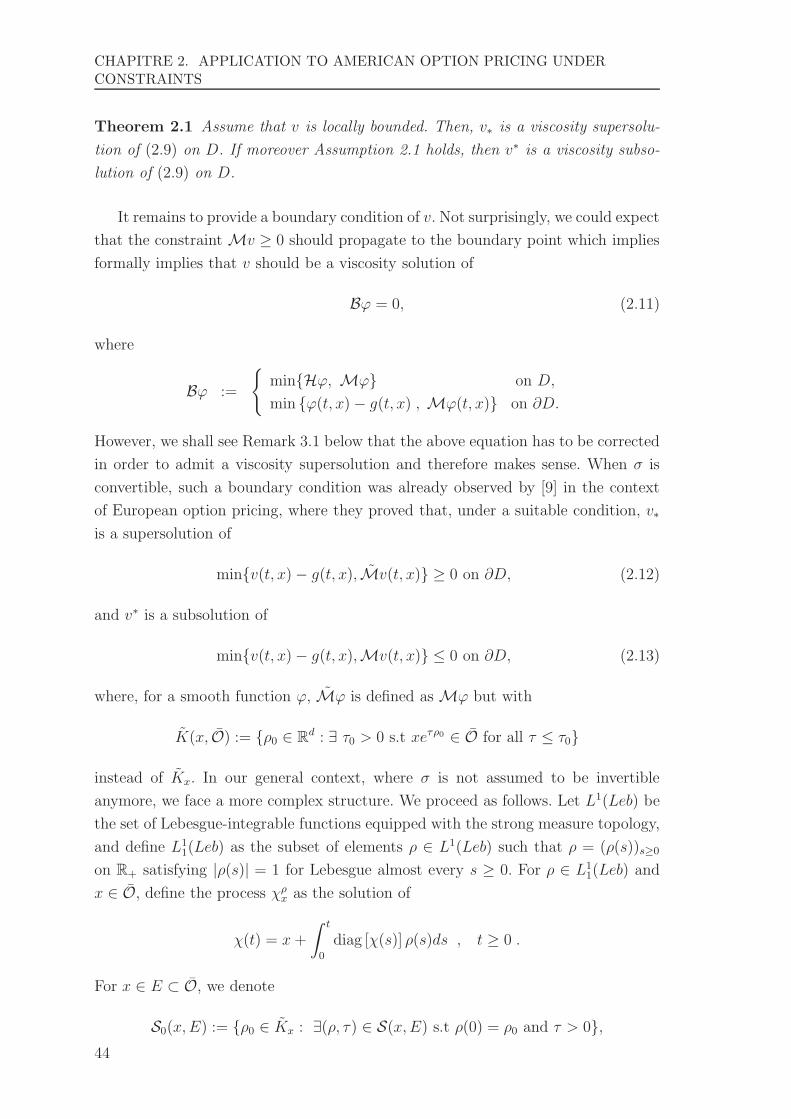
CHAPITRE 2. APPLICATION TO AMERICAN OPTION PRICING UNDER
CONSTRAINTS
Theorem 2.1 Assume that v is locally bounded. Then, v∗ is a viscosity supersolu-
tion of (2.9) on D. If moreover Assumption 2.1 holds, then v∗ is a viscosity subso-
lution of (2.9) on D.
It remains to provide a boundary condition of v. Not surprisingly, we could expect
that the constraint Mv ≥ 0 should propagate to the boundary point which implies
formally implies that v should be a viscosity solution of
Bϕ = 0, (2.11)
where
Bϕ :=
minHϕ, Mϕ on D,
min ϕ(t, x)− g(t, x) , Mϕ(t, x) on ∂D.
However, we shall see Remark 3.1 below that the above equation has to be corrected
in order to admit a viscosity supersolution and therefore makes sense. When σ is
convertible, such a boundary condition was already observed by [9] in the context
of European option pricing, where they proved that, under a suitable condition, v∗
is a supersolution of
minv(t, x)− g(t, x),Mv(t, x) ≥ 0 on ∂D, (2.12)
and v∗ is a subsolution of
minv(t, x)− g(t, x),Mv(t, x) ≤ 0 on ∂D, (2.13)
where, for a smooth function ϕ, Mϕ is defined as Mϕ but with
K(x, O) := ρ0 ∈ Rd : ∃ τ0 > 0 s.t xeτρ0 ∈ O for all τ ≤ τ0
instead of Kx. In our general context, where σ is not assumed to be invertible
anymore, we face a more complex structure. We proceed as follows. Let L1(Leb) be
the set of Lebesgue-integrable functions equipped with the strong measure topology,
and define L11(Leb) as the subset of elements ρ ∈ L1(Leb) such that ρ = (ρ(s))s≥0
on R+ satisfying |ρ(s)| = 1 for Lebesgue almost every s ≥ 0. For ρ ∈ L11(Leb) and
x ∈ O, define the process χρx as the solution of
χ(t) = x+
∫ t
0
diag [χ(s)] ρ(s)ds , t ≥ 0 .
For x ∈ E ⊂ O, we denote
S0(x, E) := ρ0 ∈ Kx : ∃(ρ, τ) ∈ S(x, E) s.t ρ(0) = ρ0 and τ > 0,44

2. THE BARRIER OPTION HEDGING
where
S(x, E) (2.14)
:= (ρ, τ) ∈ L01(Leb)× R+ : χρx(s) ∈ E, ρ(s) ∈ Kχρ
x(s) Leb. a.e. on [0, τ ].
In Lemma 3.5 below, we will show that v∗ is a supersolution of
Mdv(t, x) := infρ0∈S0(x,O)
δx(ρ0)v − ρ⊤0 diag [x]Dv = 0 on ∂D,
under the following additional assumptions :
Assumption 2.2 (i) For all x ∈ O, the closure of S0(x,O) is equal to S0(x, O).
(ii) (xn)n≥1 is a sequence in O such that
xn → x ∈ ∂O and (ρ, τ) ∈ S(x, O),
there exists a sequence (ρn, τn) → (ρ, τ) such that, up to a subsequence,
(ρn, τn) ∈ S(xn, O) for n ≥ 1,
and∫ τn
0
δχρnxn(ρn(s))ds→
∫ τ
0
δχρx(ρ(s))ds.
Assumption 2.3 There exists a map d : (0,∞)d → R such that
(i) x ∈ (0,∞)d : d(x) > 0 = O.(ii) x ∈ (0,∞)d : d(x) = 0 = ∂O.(iii) For all x ∈ ∂O, there exists r > 0 such that d ∈ C2(Br(x)).
(iv) For all x ∈ ∂O, σ(x)⊤ diag [x] Dd(x) 6= 0.
Remark 2.5 The conditions (i), (ii) and (iii) of Assumption 2.3 are automatically
satisfied when O has a smooth enough boundary, see [25]. The condition (iv) is not
required in the proof of the viscosity property stated in Theorem 2.2 below, but will
be used to prove the comparison result of Theorem 2.3.
Remark 2.6 We discuss here the relationship between the operators M,M and
Md :
1. In the case where σ is invertible, (2.10) implies that S0(x, O) = K(x, O),
which therefore leads to the coincidence of Mdv(t, x) and Mv(t, x).
2. Note that, if x ∈ O, then there exists rx > 0 such that Brx(x) ⊂ O. Then
S0(x, O) ⊃ S0(x,Brx(x)) = Kx for all x ∈ O.
Moreover, Mdv(t, x) = Mv(t, x) on T × O. We therefore only realize the
difference between Md and M as x ∈ ∂O.
45

CHAPITRE 2. APPLICATION TO AMERICAN OPTION PRICING UNDER
CONSTRAINTS
The above remark leads to the separation of the boundary into the two sub-domains
∂TD := T × O and ∂xD := [0, T ]× ∂O :
Definition 2.1 A lower semicontinuous (resp. upper semicontinuous ) function w
on [0, T ]× O is a viscosity supersolution (resp. subsolution ) of
Bdϕ = 0, (2.15)
if, for any test function ϕ ∈ C1,2([0, T ]× O) and (t0, x0) ∈ [0, T ]× O that achieves
a local minimum (resp. maximum) of w − ϕ so that (w − ϕ)(t0, x0) = 0, we have
Bdϕ(t0, x0) ≥ 0 (resp. Bϕ(t0, x0) ≤ 0),
where
Bdϕ :=
Bϕ on D ∪ ∂TD,min ϕ(t, x)− g(t, x) , Mdϕ(t, x) on ∂xD.
A locally bounded function w is a discontinuous viscosity solution of (2.15) if w∗
(resp. w∗) is a supersolution (resp. subsolution) of (2.15).
Theorem 2.2 Let Assumptions 2.1, 2.3 and 2.2 hold. Then, v is a discontinuous
viscosity solution of (2.15).
We conclude by establishing a comparison result for (2.15) which implies that v
is continuous on [0, T ) × O, with a continuous extension to [0, T ] × O, and is the
unique viscosity solution of (2.15) in a suitable class of functions. To this purpose,
we shall need the following additional assumptions :
Assumption 2.4
(i) There exists γ ∈ K ∩ [0,∞)d and λ > 1 such that λγ ∈ Kx for all x ∈ O.
(ii) There exists a constant C > 0 such that |g(t, x)| ≤ C (1 + xγ) for all (t, x) ∈[0, T ]× O.
(iii) There exists cK > 0 such that δx(ρ0) ≥ cK for all x ∈ O and ρ0 ∈ Kx.
(iv) There exists C > 0 such that, for all x, y ∈ O and ρ0 ∈ Kx, we can find ρ ∈ Ky
satisfying |ρ − ρ| ≤ C|x − y| and δy(ρ) − δx(ρ0) ≤ ǫ(x, y), where ǫ is a continuous
map satisfying ǫ(z, z) = 0 for all z ∈ (0,∞)d.
(v) Either
(v.a.) There exists L > 0 such that, for all (x, x, y, y, p, p) ∈ (0,∞)2d × R2+ × R2d :
π ∈ N(x, y, p) 6= ∅, N(x, y, p) 6= ∅ and |x− x| ≤ L−1 =⇒ ∃ π ∈ N(x, y, p) s.t.
|yπ⊤µ(x)− yπ⊤µ(x)| ≤ L|p⊤diag [x]µ(x)− p⊤diag [x]µ(x)| .
or
(v.b.) For all p, q ∈ Rd and x ∈ (0,∞)d : p⊤σ(x) = q⊤σ(x) =⇒ p⊤µ(x) = q⊤µ(x).
46

2. THE BARRIER OPTION HEDGING
Remark 2.7 1. The first condition holds whenever λγ ∈ K.
2. The condition (ii) implies that
∃ C > 0 s.t. |v(t, x)| ≤ C (1 + xγ) ∀ (t, x) ∈ [0, T ]× (0,∞)d. (2.16)
Indeed, let π ∈ A be defined by πs = γ for all t ≤ s ≤ T . Since σ is bounded, one
easily checks from the dynamics of the processes Xt,x and Y πt,x,1 that
1 +d∏
i=1
(X it,x(u))
γi ≤ C
(1 +
d∏
i=1
(xi)γi
)Y πt,x,1(u) for all u ∈ [t, T ] ,
where C > 0 depends only on |γ| and the bound on |σ|. Then, after possibly changing
the value of the constant C, (ii) of Assumption 2.4 implies
g(u,Xt,x(u)) ≤ C (1 + xγ) Y πt,x,1(u) for all u ∈ [0, T ] .
Since yY πt,x,1 = Y π
t,x,y for y > 0, we deduce (2.16) from the last inequality.
3. The condition (iii) is implied by 0 ∈ int(K). Indeed, if 0 ∈ int(K), then δx ≥ δ
where the later is uniformly strictly positive, see [39].
4. The condition (iv) is trivially satisfied if δx = δ for all x ∈ O, which is the case
when σ is invertible.
5. The condition (v) is trivially satisfied when σ is invertible. The condition (v.b.)
is natural in the case 0 ∈ int(K) as, in this case, it is equivalent to π⊤σ(x) = 0 ⇒π⊤µ(x) ≤ 0 for all π ∈ K, which is intimately related to the minimal no-arbitrage
condition : π ∈ A and Yt,x,yπ⊤σ(Xt,x) = 0 Leb×P-a.e. on [t, T ]⇒ Yt,x,yπ
⊤µ(Xt,x) ≤ 0
Leb×P-a.e. on [t, T ].
Theorem 2.3 Let Assumptions 2.1, 2.2, 2.3 and 2.4 hold. Then, v∗ = v∗ is conti-
nuous on [0, T ] × O and is the unique viscosity solution of (2.15) in the class of
non-negative functions satisfying the growth condition (ii) of Assumption 2.4.
2.4 The “face-lift” phenomenon
When σ is invertible, it can be shown under mild assumptions that the unique
viscosity solution of (2.12)-(2.13) in a suitable class, is given by g(T, ·) where
g(t, x) := supρ0∈K(x,O)
e−δ(ρ0)g(t, xeρ0) .
A standard comparison theorem, see Section 3.4 below, then implies that the boun-
dary condition can actually be written in v∗(T, ·) = v∗(T, ·) = g(T, ·). This is the
so-called “face-lift“ procedure which was already observed by [13] in the context of
European option pricing, see also [4], [7], [9] or [20].
47

CHAPITRE 2. APPLICATION TO AMERICAN OPTION PRICING UNDER
CONSTRAINTS
In our general context, where σ is not assumed to be invertible anymore, standard
optimal control arguments actually show that it should be related to the determi-
nistic control problem
g(t0, x) := sup(ρ,τ)∈S(x,O)
e−
∫ τ0δχρx(s)
(ρ(s))dsg(t0, χ
ρx(τ)),
which is well defined on O by (2.14).
Note that, in the case where σ is invertible, (2.10) implies that it can be rewritten
in
sup(ρ,τ)∈S(x,O)
e−∫ τ0 δ(ρ(s))dsg(t0, χ
ρx(τ))
whose value function is easily seen to coincide with g(t0, ·) by using the fact that δ
is convex and homegenous of degree one, and g ≥ 0.
We now make precise the above discussion in the two following Corollaries. The
first one actually states that g can be replaced by g in the definition of H and in
the terminal condition.
Corollary 2.2 Let Assumption 2.1 and (i)-(iv) of Assumption 2.4 hold. Assume
further that :
(i) For each x ∈ O, the map t ∈ [0, T ] 7→ g(t, x) is continuous.
(ii) The map x ∈ O 7→ supδx(ρ0), ρ0 ∈ Kx is locally bounded.
Then, v is a discontinuous viscosity solution of (2.15) and satisfies the boundary
condition
v∗(T, ·) = v∗(T, ·) = g(T, ·) on O. (2.17)
If moreover, (v) of Assumption 2.4 hold, then it is the unique viscosity solution of
(2.15)-(2.17), in the class of non-negative functions satisfying the growth condition
(2.16).
3 Proof of the PDE characterization
From now on, we assume that v is locally bounded.
3.1 The supersolution property
We start with the supersolution property of Theorem 2.2.
Lemma 3.1 The map v∗ is a viscosity supersolution of Hϕ = 0 on [0, T )×O.
48
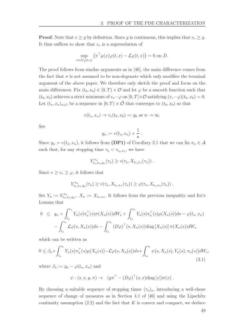
3. PROOF OF THE PDE CHARACTERIZATION
Proof. Note that v ≥ g by definition. Since g is continuous, this implies that v∗ ≥ g.
It thus suffices to show that v∗ is a supersolution of
supπ∈Nϕ(t,x)
(π⊤µ(x)ϕ(t, x)−Lϕ(t, x)
)= 0 on D.
The proof follows from similar arguments as in [46], the main difference comes from
the fact that σ is not assumed to be non-degenate which only modifies the terminal
argument of the above paper. We therefore only sketch the proof and focus on the
main differences. Fix (t0, x0) ∈ [0, T )×O and let ϕ be a smooth function such that
(t0, x0) achieves a strict minimum of v∗−ϕ on [0, T ]×O satisfying (v∗−ϕ)(t0, x0) = 0.
Let (tn, xn)n≥1 be a sequence in [0, T )× O that converges to (t0, x0) so that
v(tn, xn) → v∗(t0, x0) =: y0 as n→ ∞.
Set
yn := v(tn, xn) +1
n.
Since yn > v(tn, xn), it follows from (DP1) of Corollary 2.1 that we can fin πn ∈ Asuch that, for any stopping time τn < τtn,xn, we have
Y πntn,xn,yn(τn) ≥ v(τn, Xtn,xn(τn)) .
Since v ≥ v∗ ≥ ϕ, it follows that
Y πntn,xn,yn(τn) ≥ v(τn, Xtn,xn(τn)) ≥ ϕ(τn, Xtn,xn(τn)) .
Set Yn := Y πntn,xn,yn, Xn := Xtn,xn. It follows from the previous inequality and Ito’s
Lemma that
0 ≤ yn +
∫ τn
tn
Yn(s)π⊤n (s)σ(Xn(s))dWs +
∫ τn
tn
Yn(s)π⊤n (s)µ(Xn(s))ds− ϕ(tn, xn)
−∫ τn
tn
Lϕ(s,Xn(s))ds−∫ τn
tn
(Dϕ)⊤(s,Xn(s))diag [Xn(s)] σ(Xn(s))dWs
which can be written as
0 ≤ βn+
∫ τn
tn
Yn(s)π⊤n (s)µ(Xn(s))−Lϕ(s,Xn(s))ds+
∫ τn
tn
ψ(s,Xn(s), Yn(s), πn(s))dWs,
(3.1)
where βn := yn − ϕ(tn, xn) and
ψ : (s, x, y, π) → (yπ⊤ − (Dϕ)⊤(s, x)diag [x])σ(x) .
By choosing a suitable sequence of stopping times (τn)n, introducing a well-chose
sequence of change of measures as in Section 4.1 of [46] and using the Lipschitz
continuity assumption (2.2) and the fact that K is convex and compact, we deduce
49
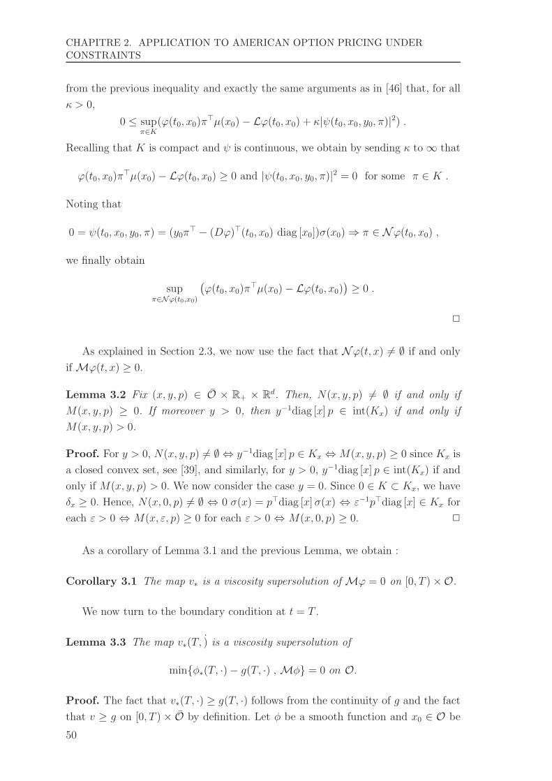
CHAPITRE 2. APPLICATION TO AMERICAN OPTION PRICING UNDER
CONSTRAINTS
from the previous inequality and exactly the same arguments as in [46] that, for all
κ > 0,
0 ≤ supπ∈K
(ϕ(t0, x0)π⊤µ(x0)− Lϕ(t0, x0) + κ|ψ(t0, x0, y0, π)|2) .
Recalling that K is compact and ψ is continuous, we obtain by sending κ to ∞ that
ϕ(t0, x0)π⊤µ(x0)− Lϕ(t0, x0) ≥ 0 and |ψ(t0, x0, y0, π)|2 = 0 for some π ∈ K .
Noting that
0 = ψ(t0, x0, y0, π) = (y0π⊤ − (Dϕ)⊤(t0, x0) diag [x0])σ(x0) ⇒ π ∈ Nϕ(t0, x0) ,
we finally obtain
supπ∈Nϕ(t0,x0)
(ϕ(t0, x0)π
⊤µ(x0)− Lϕ(t0, x0))≥ 0 .
2
As explained in Section 2.3, we now use the fact that Nϕ(t, x) 6= ∅ if and only
if Mϕ(t, x) ≥ 0.
Lemma 3.2 Fix (x, y, p) ∈ O × R+ × Rd. Then, N(x, y, p) 6= ∅ if and only if
M(x, y, p) ≥ 0. If moreover y > 0, then y−1diag [x] p ∈ int(Kx) if and only if
M(x, y, p) > 0.
Proof. For y > 0, N(x, y, p) 6= ∅ ⇔ y−1diag [x] p ∈ Kx ⇔ M(x, y, p) ≥ 0 since Kx is
a closed convex set, see [39], and similarly, for y > 0, y−1diag [x] p ∈ int(Kx) if and
only if M(x, y, p) > 0. We now consider the case y = 0. Since 0 ∈ K ⊂ Kx, we have
δx ≥ 0. Hence, N(x, 0, p) 6= ∅ ⇔ 0 σ(x) = p⊤diag [x] σ(x) ⇔ ε−1p⊤diag [x] ∈ Kx for
each ε > 0 ⇔ M(x, ε, p) ≥ 0 for each ε > 0 ⇔ M(x, 0, p) ≥ 0. 2
As a corollary of Lemma 3.1 and the previous Lemma, we obtain :
Corollary 3.1 The map v∗ is a viscosity supersolution of Mϕ = 0 on [0, T )×O.
We now turn to the boundary condition at t = T .
Lemma 3.3 The map v∗(T, ) is a viscosity supersolution of
minφ∗(T, ·)− g(T, ·) , Mφ = 0 on O.
Proof. The fact that v∗(T, ·) ≥ g(T, ·) follows from the continuity of g and the fact
that v ≥ g on [0, T )× O by definition. Let φ be a smooth function and x0 ∈ O be
50

3. PROOF OF THE PDE CHARACTERIZATION
such that x0 achieves a strict minimum of v∗(T, ·)−φ and v∗(T, x0)−φ(x0) = 0. Let
(sn, ξn)n be a sequence in [0, T )×O satisfying
(sn, ξn) −→ (T, x0) , sn < T and v∗(sn, ξn) −→ v∗(T, x0) .
For all n ∈ N and k > 0, we define
ϕkn(t, x) := φ(x)− k
2|x− x0|2 + k
T − t
T − sn.
Notice that 0 ≤ (T − t)(T − sn)−1 ≤ 1 for t ∈ [sn, T ], and therefore
limk→0
lim supn→∞
sup(t,x)∈[sn,T ]×Br(x0)
|ϕkn(t, x)− φ(x)| = 0 , (3.2)
where r > 0 is such that Br(x0) ⊂ O. Next, let (tkn, xkn) be a sequence of local
minimizers of v∗ − ϕkn on [sn, T ]×Br(x0) and set ekn := (v∗ − ϕkn)(tkn, x
kn). Following
line by line the arguments of the proof of Lemma 20 in [7], one easily checks that,
after possibly passing to a subsequence,
for all k > 0 , (tkn, xkn) −→ (T, x0) , (3.3)
for all k > 0 , tkn < T for sufficiently large n , (3.4)
v∗(tkn, x
kn) −→ v∗(T, x0) = φ(x0) as n→ ∞ and k → 0 . (3.5)
Notice that (3.3) and a standard localization argument implies that we may
assume that xkn ∈ Br(x0) for all n ≥ 1 and k > 0. It then follows from (3.4) that, for
all k > 0, (tkn, xkn) is a sequence of local minimizers of v∗ − ϕkn on [sn, T ) × Br(x0).
Also, notice that (3.2), (3.3) and (3.5) imply
for all k > 0 , Dϕkn(tkn, x
kn) = Dφ(xkn)− k(xkn − x0) → Dφ(x0) , (3.6)
and limk→0
limn→∞
ekn = 0 . (3.7)
It then follows from Theorem 2.2, recall the convention sup ∅ = −∞, (3.4) and
the fact that (tkn, xkn) is a local minimizer for v∗ − ϕkn that, for sufficiently large n,
we can find πkn ∈ K such that
v∗(tkn, x
kn)(π
kn)
⊤σ(xkn) = Dϕkn(tkn, x
kn)
⊤diag[xkn]σ(xkn) .
Since K is compact, we can assume that πkn → π ∈ K as n → ∞ and then k → 0.
Taking the limit as n→ ∞ and then as k → 0 in the previous inequality, and using
(3.3), (3.5), (3.6), as well as the continuity of x 7→ diag [x] σ(x) thus implies that
v∗(T, x0)π⊤σ(x0) = Dφ(x0)
⊤diag [x0] σ(x0) .
Appealing to Lemma 3.2 then implies the required result. 2
In order to prove the boundary condition on ∂xD, we need following Lemma :
51

CHAPITRE 2. APPLICATION TO AMERICAN OPTION PRICING UNDER
CONSTRAINTS
Lemma 3.4 Let (t, x) ∈ D. Then
v∗(t, x) = sup(ρ,τ)∈S(x,O)
e−
∫ τ0 δ
χρx(s)
(ρ(s))dsv∗(t, χ
ρx(τ)). (3.8)
Proof. We start with the case (t, x) ∈ D. It follows from Assumption 2.2 and the
lower semicontinuity of v∗ that
sup(ρ,τ)∈S(x,O)
e−
∫ τ0 δ
χρx(s)
(ρ(s))dsv∗(t, χ
ρx(τ)) = sup
(ρ,τ)∈S(x,O)
e−
∫ τ0 δ
χρx(s)
(ρ(s))dsv∗(t, χ
ρx(τ)).
It suffices to show that
v∗(t, x) = sup(ρ,τ)∈S(x,O)
e−
∫ τ0 δ
χρx(s)
(ρ(s))dsv∗(t, χ
ρx(τ)).
We fix (ρ, τ) ∈ S(x,O) so that τ > 0, denote the map
w : r → w(r) = e−
∫ τ0 δ
χρx(s)
(ρ(s))dsv∗(t, χ
ρx(r))
defined on [0, τ ]. We shall prove that w(0) ≥ w(τ).
The fact that χρx(s) ∈ O for all s ≤ τ , together with Corollary 3.1, implies that
v∗ is a supersolution of
infρ0∈Kx
δx(ρ0)ϕ− ρ⊤0 diag [x]Dϕ ≥ 0 on t × Iρx ,
where Iρx := χρx(r) : r ∈ [0, τ ].The map w therefore is a supersolution of
−Dw ≥ 0 on [0, τ ].
This allows us to prove the required result by following the steps below :
1. For any r0 ∈ (0, τ ], there exist a(r0) ≥ 0 satisfying
0 ≤ a(r0) < r0
and
w(r0) ≤ w(a) for a ∈ [a(r0), r0].
Given ǫ > 0, we define wǫ(r) := w(r)−ǫr for r ∈ [0, τ ]. Then wǫ is a supersolu-
tion of −Dwǫ ≥ ǫ on [0, τ ]. This means that for a smooth function ϕ such that
r0 achieves a strict minimum of wε − ϕ on [0, τ ] satisfying (wǫ − ϕ)(r0) = 0,
we have Dϕ(r0) ≤ −ǫ. This implies that there exists a(r0) ≥ 0 such that
a(r0) < r0 and ϕ is strictly decreasing on [a(r0), r0]. We intend to prove that
wǫ(a) > wǫ(r0) for all a ∈ [a(r0), r0].
52

3. PROOF OF THE PDE CHARACTERIZATION
Assume to the contrary that there exists a ∈ [a(r0), r0) such that
wǫ(a) ≤ wǫ(r0). (3.9)
Note that the map waǫ (r) ≡ wǫ(a) solves the equation Dϕ = 0 on [a, r0] with
the boundary conditions waǫ (a) = waǫ (r0) = wǫ(a). It follows from a standard
comparison argument and (3.9) that
sup[a,r0]
(waǫ − wǫ) ≤ maxwaǫ (a)− wǫ(a), waǫ (r0)− wǫ(r0) ≤ 0.
Then,
wǫ(a) = waǫ (r0) ≤ wǫ(r0).
Recalling that the test function ϕ is strictly decreasing on [a, r0], we have
wǫ(a)− ϕ(a) < wǫ(r0)− ϕ(r0),
which leads to a contradiction of the strict minimum property of wǫ−ϕ at r0.
2. We now prove that
wǫ(r0) ≥ lim infb→r0,b>r0
wǫ(b) for r0 ∈ [0, τ).
Assume to the contradiction that there exists b(r0) > r0 such that
wǫ(r0) < wǫ(b) for all b ∈ (r0, b(r0)]. (3.10)
In view of step 1., there exists a(r0) < r0 such that
wε(a) ≥ wε(r0) for all a ∈ [a(r0), r0].
This, together with (3.10), implies that a test function
φ(r) := wǫ(r0)
satisfies
min[a(r0),b(r0)]
(wǫ − φ) = wǫ(r0)− φ(r0) = 0,
but Dφ(r0) = 0, which leads to a contradiction of the supersolution property
of wǫ stated in step 1.
3. In order to complete the proof, we set
τ0 = infs ≤ τ : w(r) ≥ w(τ) for all r ∈ [s, τ ], (3.11)
and show that τ0 = 0. Note that τ0 ≤ a(τ) < τ , where the function a(·) is
defined in step 1. Assume that τ0 > 0.
53

CHAPITRE 2. APPLICATION TO AMERICAN OPTION PRICING UNDER
CONSTRAINTS
It then follows from step 1 and step 2, applied r0 = τ0, that there exists a < τ0
such that
w(r) ≥ w(τ0) for all r ∈ [a, τ0),
w(τ0) ≥ lim infb→τ0,b>τ0
w(b) ≥ w(τ),
which leads to a contradiction of the definition of τ0. The required result follows
from step 2. with r0 = 0.
We have just prove the equality (3.8) when (t, x) ∈ D. We could show that this
equality is also valired when (t, x) ∈ ∂TD, by taking limits as t → T . It remains to
consider the case where (t, x) ∈ ∂xD. Let (tn, xn)n≥1 be a sequence in D such that
(tn, xn) → (t, x) and v(tn, xn) → v∗(t, x). Fix (ρ, τ) ∈ S(x, O). It follows from the
condition (ii) of Assumption 2.2 that there exists (ρn, τn) ∈ S(xn, O) for all n ≥ 1
satisfying (ρn, τn) → (ρ, τ). Then,
v∗(tn, xn) ≥ e−
∫ τn0
δχρnxn (s)
(ρn(s))dsv∗(tn, χ
ρnxn(τn)),
which leads to the required result by sending n→ ∞. 2
We now provide a boundary condition on ∂xD :
Lemma 3.5 The map v∗ is a viscosity supersolution of
Mdϕ(t, x) = 0 on D.
Proof. Let (t, x) ∈ D and ϕ be a C2 function such that
0 = (v∗ − ϕ)(t, x) = minD
(v∗ − ϕ).
We fix (ρ, τ) ∈ S(x, O). It follows from (3.8) that
ϕ(t, x) = v∗(t, x) ≥ e−
∫ r0 δχρ
x(s)(ρ(s))ds
v∗(t, χρx(r)) ≥ e
−∫ r0 δχρ
x(s)(ρ(s))ds
ϕ(t, χρx(r))
for all r ≤ τ. Dividing by r and sending r → 0, leads to the required result. 2
Remark 3.1 Note that, under Assumption 2.3 the map v∗ can not be a supersolu-
tion of Mϕ(t, x) = 0 on ∂xD. Assume to the contradiction that for all (t0, x0) ∈ ∂xD
and a smooth function ϕ such that minD(v∗ − ϕ) = (v∗ − ϕ)(t0, x0) = 0 then
Mϕ(t0, x0) ≥ 0.
Let (t0, x0) ∈ ∂xD and a smooth function ϕ such that (t0, x0) is a minimum of
v∗ − ϕ. In view of Assumption 2.3, (t0, x0) is also a minimum of v∗ − ϕε, where
ϕε(t, x) := ϕ(t, x)− ε−1d(x) for ε > 0. This implies that
infρ0∈Kx0
δx0(ρ)ϕ(t0, x0)− ρ⊤0 diag [x0] (Dϕ(t0, x0)− ε−1d(x0)) ≥ 0. (3.12)
Let ρ0 ∈ Kx0\S0(x0, O), then there exist a sequence τn → 0 and ρ ∈ L11(Leb)
such that d(χρx0(τn)) < 0 and ρ(0) = ρ0, recall Assumption 2.3. This implies that
ρ⊤0 diag [x0]Dd(x0) < 0, which leads to a contradiction of (3.12) when ε comes to 0.
54

3. PROOF OF THE PDE CHARACTERIZATION
3.2 The subsolution property
We now turn to the subsolution property of Theorem 2.2.
Lemma 3.6 Under Assumption 2.1, the map v∗ is a viscosity subsolution of
minHϕ , Mϕ = 0 on [0, T )×O.
Proof. Fix (t0, x0) ∈ [0, T ) × O and let ϕ be a smooth function such that (t0, x0)
achieves a strict maximum of v∗ − ϕ on [0, T ] × O satisfying (v∗ − ϕ)(t0, x0) = 0.
We assume that
min Hϕ(t0, x0) Mϕ(t0, x0) := 2ε > 0 ,
and work towards a contradiction. Note that v∗(t0, x0) = ϕ(t0, x0) > 0 since g ≥ 0.
In view of Lemma 3.2, this implies that ϕ(t0, x0)−1diag [x0]Dϕ(t0, x0) ∈ int(Kx0). It
then follows from Assumption 2.1 that we can find r > 0 and a Lipschitz continuous
map π such that
minyπ(x, y,Dϕ(t, x))⊤µ(x)−Lϕ(t, x) , y − g(t, x)
> ε
and, for (t, x, y) ∈ Br(t0, x0)× Br(ϕ(t, x)) ⊂ D × (0,∞),
π(x, y,Dϕ(t, x)) ∈ N(x, y,Dϕ(t, x)). (3.13)
Let (tn, xn)n be a sequence in Br(t0, x0) such that v(tn, xn) → v∗(t0, x0) and set
yn := v(tn, xn)− n−1 so that yn > 0 for n large enough. Without loss of generality,
we can assume that yn ∈ Br(ϕ(tn, xn)) for each n. Let (Xn, Y n) denote the solution
of (2.1) and (2.3) associated to the Markovian control π(Xn, Y n, Dϕ(·, Xn)) and
the initial conditions (Xn(tn), Yn(tn)) = (xn, yn). Note that these processes are well
defined on [tn, τn] where
τn := inf t ≥ tn : (t, Xn(t)) /∈ Br(t0, x0) or |Y n(t)− ϕ(t, Xn(t))| ≥ r .
Moreover, it follows from the definition of (t0, x0) as a strict maximum point of v∗−ϕthat
(v∗ − ϕ)(τn, Xn(τn)) < −ζ or |Y n(τn)− ϕ(τn, X
n(τn))| ≥ r (3.14)
for some ζ > 0. Since v∗ ≤ ϕ, applying Ito’ Lemma to Y n−ϕ(·, Xn), recalling (3.13)
and using a standard comparison Theorem for stochastic differential equations shows
that
Y n(τn)− v(τn, Xn(τn)) ≥ Y n(τn)− ϕ(τn, X
n(τn) ≥ r
on |Y n(τn)− ϕ(τn, Xn(τn))| ≥ r .
55

CHAPITRE 2. APPLICATION TO AMERICAN OPTION PRICING UNDER
CONSTRAINTS
The same arguments combined with (3.14) also implies that
Y n(τn)− v(τn, Xn(τn)) ≥ yn − ϕ(tn, xn) + ζ on |Y n(τn)− ϕ(τn, X
n(τn))| < r .
Since yn − ϕ(tn, xn) → 0, combining the two last assertions shows that Y n(τn) −v(τn, X
n(τn)) > 0 for n large enough. Moreover, it follows from (3.13) that Y n >
g(·, Xn) on [tn, τn]. Since yn < v(tn, xn), this contradicts (DP2) of Corollary 2.1.
2
Lemma 3.7 Let Assumption 2.1, 2.2 and 2.3 hold. Fix (t0, x0) ∈ ∂TD ∪ ∂xD and
assume that there exists a smooth function φ such that Mφ(t0, x0) > 0 and (t0, x0)
achieves a strict local maximum of v∗ − φ. Then,
v∗(t0, x0) ≤ g(t0, x0).
Proof. 1. We first prove the required result when (t0, x0) ∈ ∂xD. Since g is conti-
nuous and Mφ(t0, x0) > 0, it follows from Lemma 3.2, and Assumption 2.1, 2.3 that
we can find r, η > 0 and a Lipschitz continuous map π such that
d(x0) = 0, 0 ≤ d(x) < ǫλ on Br(x0) ∩ O, (3.15)
and, for (t, x, y) ∈ [t0, t0 + r]× (Br(x0) ∩ O)× Br(ϕ(t0, x0)),
π(x, y,Dϕ(t, x)) ∈ N(x, y,Dϕ(t, x)), ϕ(t, x)− g(t, x) ≥ η, (3.16)
where
ϕ(t, x) := φ(t, x) + λd(x)− d2(x)
ǫ+
1
2|x− x0|2
with ǫ, λ > 0 small enough.
In view of (i) and (iv) of Assumption 2.2, we also have, after possibly changing
r > 0 and sending ǫ to 0,
yπ(x, y,Dϕ(t, x))⊤µ(x)− Lϕ(t, x) ≥ η (3.17)
for (t, x, y) ∈ [t0, t0 + r]× (Br(x0) ∩ O)×Br(ϕ(t0, x0)) =: B.
The fact that v∗ − ϕ achieves a strict local maximum at (t0, x0), recall (3.15), and
that g(t, x) = v(t, x) on ∂xD imply that
sup∂pB
(v − ϕ) < 0, (3.18)
where ∂pB := t0 + r × (Br(x0) ∩O) ∪ [t0, t0 + r]× ∂(Br(x) ∩ O).
Let (tn, xn)n be a sequence in [0, T )×O converging to (t0, x0) such that
v(tn, xn) → v∗(t0, x0) .
56

3. PROOF OF THE PDE CHARACTERIZATION
and let (tn, xn) be a strict maximum point of v∗−ϕ on [tn−n−1, tn]×O. One easily
checks that tn < T and that (tn, xn) → (t0, x0).
Obviously, we can assume that (tn, xn) ∈ B. Let (Xn, Y n) denote the solution of
(2.1) and (2.3) associated to the Markovian control π(Xn, Y n, Dϕ(·, Xn)) and the
initial conditions (Xn(tn), Yn(tn)) = (xn, yn). Note that these processes are well
defined on [tn, τn] where
τn := inft ≥ tn : (t, Xn(t)) /∈ B or |Y n(t)− ϕ(t, Xn(t))| ≥ r
.
Applying Ito’ Lemma to Y n − ϕ(·, Xn) and arguing as in the proof of Lemma 3.6,
we then deduce that (3.17) and (3.18) lead to a contradiction to (DP2) of Corollary
2.1.
2. The case where (t0, x0) ∈ T × O can be treated similarly by similar argument
as in previous step, after replacing ϕ by (t, x) 7→ φ(t, x) +√T − t. 2
3.3 A comparison result
In this section, we prove Theorem 2.3. This is a consequence of the following
comparison result and the growth property for v which was derived in Remark 2.7.
Proposition 3.1 Let Assumption 2.4 hold. Let V (resp. U) be a non-negative lower-
semicontinuous (resp. upper-semicontinuous) locally bounded map on [0, T ]×O satis-
fying (2.16). Assume that V (resp. U) is a viscosity supersolution (resp. subsolution)
of (2.15) on [0, T ]× O. Then, V ≥ U on [0, T ]× O.
In order to prove Proposition 5.1, we need a technical Lemma :
Lemma 3.8 Let Assumption 2.3 and (iv) of Assumption 2.4 hold. Fix x0 ∈ ∂O.
Then there exists (ρ, τ) ∈ S(x0, O) such that
Dd(x0)⊤diag [x0] ρ0 > 0 and ρ(0) = ρ0. (3.19)
Moreover, we could choose τ > 0 small enough such that (ρ, τ) ∈ S(x, O) for all
x ∈ Br(x0) with some r > 0.
Proof. Note that the condition (iv) of Assumption 2.3 allows us to define ρ0 :=
σ(x0)ρ0/|σ(x0)ρ0|, where ρ0 satisfies σ(x0)⊤diag [x0]Dd(x0)ρ0 > 0. It then follows
from (iv) of Assumption 2.4 that we can find r > 0 and a Lipschitz continuous map
ρ such that
Dd(x)⊤diag [x0] ρ0 > 0 and δx(ρ(x)) <∞ ∀ x ∈ Br(x0) ∩ O,
define χ as χρx0 for the Markovian control ρ = ρ(χ) and take ρ(s) = ρ(χ(s)).
57

CHAPITRE 2. APPLICATION TO AMERICAN OPTION PRICING UNDER
CONSTRAINTS
It remains to prove that there exists τ > 0 such that
χρx(s) ∈ O for s ≤ τ and x ∈ Br(x0) ∩ O.
The fact that χρx(s) = x+sdiag [x] ρ+o(s) implies that there exists x ∈ Br(x0) such
that
d(χρx(s)) = d(x) + sDd(x)⊤diag [x] ρ+ o(s).
This leads to required result by taking τ small enough. 2
Proof of Proposition 5.1
1. As usual, we first fix κ > 0 and introduce the functions U(t, x) := eκtU(t, x),
V (t, x) := eκtV (t, x) and g(t, x) := eκtg(t, x).
Let λ > 1 and γ ∈ O be as in Assumption 2.4. Let β be defined by β(t, x) =
eτ(T−t)(1 + xλγ
), for some τ > 0 to be chosen below, and observe that the fact that
δx ≥ 0 and λγ ∈ Kx for all x ∈ O implies that, for all (t, x) ∈ [0, T ]× O,
Mβ(t, x) = infρ0∈Kx
(δx(ρ0) + xλγ [δx(ρ0)− ρ⊤0 (λγ)]
)eτ(T−t) ≥ 0. (3.20)
Moreover, one easily checks, by using the fact that µ and σ are bounded, and K is
compact, that we can choose τ large enough so that, on [0, T ]× O,
−2L|Dβ(t, x)⊤diag [x]µ(x)|+ κβ(t, x)−Lβ(t, x) ≥ 0,
κβ(t, x)− ∂tβ(t, x)− 12Tr [a(x)D2β(t, x)] ≥ 0,
(3.21)
where a(z) := diag [z] σ(z)σ(z)⊤diag [z], and L is as in (v.a) of Assumption 2.4 if it
holds and L = 0 otherwise.
2. In order to show that U ≤ V , we argue by contradiction. We therefore assume
that
sup[0,T ]×O
(U − V ) > 0 (3.22)
and work towards a contradiction.
2.1. Using the growth condition on U and V , and (5.4), we deduce that
0 < 2m := sup[0,T ]×O
(U − V − 2αβ) <∞ (3.23)
for α > 0 small enough. Fix ε > 0 and let f be defined on O by
f(x) =d∑
i=1
(xi)−2 . (3.24)
Arguing as in the proof of Proposition 6.9 in [9], see also below for similar arguments,
we obtain that
Φε := U − V − 2(αβ + εf)
58

3. PROOF OF THE PDE CHARACTERIZATION
admits a maximum (tε, xε) on [0, T ]× O, which, for ε > 0 small enough, satisfies
Φε(tε, xε) ≥ m > 0 , (3.25)
as well as
lim supε→0
ε (|f(xε)|+ |diag [xε]Df(xε)|+ |Lf(xε)|) = 0 . (3.26)
2.2. It follows Lemma 3.8 that there exists (ρε, τε) ∈ S(xε, O) and rε > 0 such that
ρε = 0 if xε ∈ O,Dd(x)⊤diag [xε] ρε > 0 if xε ∈ ∂O,
χρεx (s) ∈ O for s ≤ τε,
(3.27)
for all x ∈ Brε(xε).
For n ≥ 1 and ζ ∈ (0, 1) such that ζ/n ≤ τε, we then define the function Ψεn,ζ on
[0, T ]× (0,∞)2d by
Ψεn,ζ(t, x, y) := Θ(t, x, y)− ε(f(x) + f(y))
−ζ(|x− xε|2 + |t− tε|2)− n2|χρεx (ζ/n)− y|2 ,
where
Θ(t, x, y) := U(t, x)− V (t, y)− α (β(t, x) + β(t, y)) .
It follows from the growth condition on U and V that Ψεn,ζ attains its maximum at
some (tεn, xεn, y
εn) ∈ [0, T ]× O2. From now, we define χεn := χρεxεn and χ1 := χρε1 . Note
that
χεn = diag [xεn]χ1. (3.28)
Moreover, the inequality Ψεn,ζ(t
εn, x
εn, y
εn) ≥ Ψε
n,ζ(tε, xε, χρεxε(ζ/n)) implies that
Θ(tεn, xεn, y
εn) ≥ Θ(tε, xε, χ
ρεxε(ζ/n))− 2εf(xε) + n2|χεn(ζ/n)− yεn|2
+ζ(|xεn − xε|2 + |tεn − tε|2
)+ ε (f(xεn) + f(yεn)) .
Using the growth property of U and V again, we deduce that the term on the second
line is bounded in n so that, up to a subsequence,
χεn(ζ/n), yεn −−−→
n→∞xε ∈ O and tεn −−−→
n→∞tε ∈ [0, T ] .
Recalling similarly as Lemma 3.4 and using the fact that (ρε, τε) ∈ S(xε, O) show
that
V (tε, xε) ≥ V (tε, χρεxε(ζ/n))e
−∫ ζ/n0
δχρεxε (s)
ρε(s)ds.
59

CHAPITRE 2. APPLICATION TO AMERICAN OPTION PRICING UNDER
CONSTRAINTS
This, together with the maximum property of (tε, xε), implies that
0 ≥ Φε(tε, xε)− Φε(tε, xε)
≥ lim supn→∞
(|χεn(ζ/n)− yεn|2 + ζ
(|xεn − xε|2 + |tεn − tε|2
)).
We get
(a) n2|χεn(ζ/n)− yεn|2 + ζ(|xεn − xε|2 + |tεn − tε|2
)−−−→n→∞
0 ,
(b) U(tεn, xεn)− V (tεn, y
εn) −−−→
n→∞
(U − V
)(tε, xε) ≥ m+ 2αβ(tε, xε) + 2εf(xε) ,
where we used (5.5) for the last assertion.
3.1. We now show that, after possibly passing to a subsequence,
yεn ∈ O. (3.29)
Note that, above result is true when xε ∈ O. It remains to show it in the case
xε ∈ ∂O. It follows from (a) that
yεn = xεn +ζ
ndiag [xεn] ρε + o(n−1),
which implies that
d(yεn) = d(xεn) +ζ
n(Dd(xεn)
⊤diag [xεn] ρε + ǫn),
for some ǫn → 0 as n→ ∞. Then, (3.29) follows from (3.27).
3.2. Assume that, after possibly passing to a subsequence,
minM(xεn, U(t
εn, x
εn), p
εn
), U(tεn, x
εn)− g(tεn, x
εn)
≤ 0
minM(yεn, V (tεn, y
εn), q
εn
), V (tεn, y
εn)− g(tεn, y
εn)
≥ 0 ,
where
pεn := 2n2diag[χ1(ζ/n)
](χεn(ζ/n)− yεn) + 2ζ(xεn − xε) + αDβ(tεn, x
εn) + εDf(xεn)
qεn := 2n2(χεn(ζ/n)− yεn)− αDβ(tεn, yεn)− εDf(yεn) .
Assuming that, after possibly passing to a subsequence, U(tεn, xεn) ≤ g(tεn, x
εn) for all
n ≥ 1, we get a contradiction to (b) since V (tεn, yεn) ≥ g(tεn, y
εn) so that passing to
the limit, recall (a) and the fact that g is continuous, implies U(tεn, xε) ≤ g(tεn, xε) ≤V (tεn, xε).
We can therefore assume that U(tεn, xεn) > g(tεn, x
εn) for all n. Using the two above
inequalities, we then deduce that
0 ≥M(xεn, U(t
εn, x
εn), p
εn
)−M
(yεn, V (tεn, y
εn), q
εn
),
60
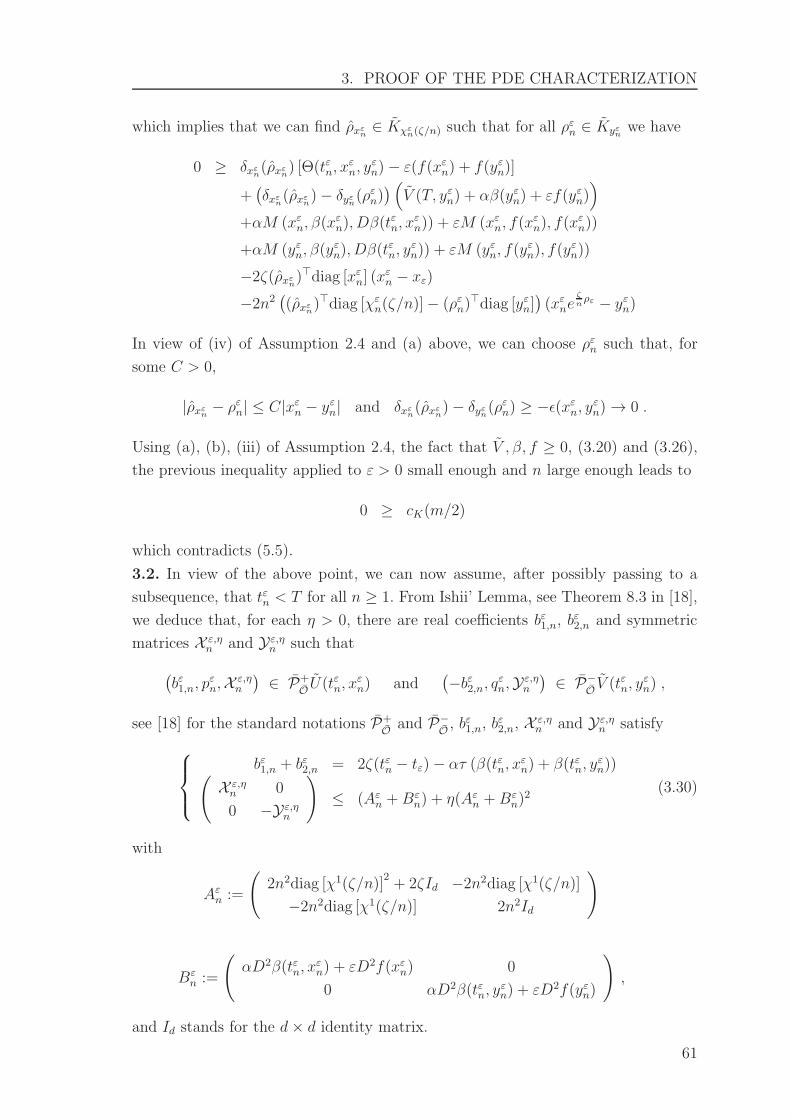
3. PROOF OF THE PDE CHARACTERIZATION
which implies that we can find ρxεn ∈ Kχεn(ζ/n) such that for all ρεn ∈ Kyεn we have
0 ≥ δxεn(ρxεn) [Θ(tεn, xεn, y
εn)− ε(f(xεn) + f(yεn)]
+(δxεn(ρxεn)− δyεn(ρ
εn)) (V (T, yεn) + αβ(yεn) + εf(yεn)
)
+αM (xεn, β(xεn), Dβ(t
εn, x
εn)) + εM (xεn, f(x
εn), f(x
εn))
+αM (yεn, β(yεn), Dβ(t
εn, y
εn)) + εM (yεn, f(y
εn), f(y
εn))
−2ζ(ρxεn)⊤diag [xεn] (x
εn − xε)
−2n2((ρxεn)
⊤diag [χεn(ζ/n)]− (ρεn)⊤diag [yεn]
)(xεne
ζnρε − yεn)
In view of (iv) of Assumption 2.4 and (a) above, we can choose ρεn such that, for
some C > 0,
|ρxεn − ρεn| ≤ C|xεn − yεn| and δxεn(ρxεn)− δyεn(ρεn) ≥ −ǫ(xεn, yεn) → 0 .
Using (a), (b), (iii) of Assumption 2.4, the fact that V , β, f ≥ 0, (3.20) and (3.26),
the previous inequality applied to ε > 0 small enough and n large enough leads to
0 ≥ cK(m/2)
which contradicts (5.5).
3.2. In view of the above point, we can now assume, after possibly passing to a
subsequence, that tεn < T for all n ≥ 1. From Ishii’ Lemma, see Theorem 8.3 in [18],
we deduce that, for each η > 0, there are real coefficients bε1,n, bε2,n and symmetric
matrices X ε,ηn and Yε,η
n such that
(bε1,n, p
εn,X ε,η
n
)∈ P+
OU(tεn, x
εn) and
(−bε2,n, qεn,Yε,η
n
)∈ P−
OV (tεn, y
εn) ,
see [18] for the standard notations P+O
and P−O, bε1,n, b
ε2,n, X ε,η
n and Yε,ηn satisfy
bε1,n + bε2,n = 2ζ(tεn − tε)− ατ (β(tεn, xεn) + β(tεn, y
εn))(
X ε,ηn 0
0 −Yε,ηn
)≤ (Aεn +Bε
n) + η(Aεn +Bεn)
2(3.30)
with
Aεn :=
(2n2diag [χ1(ζ/n)]
2+ 2ζId −2n2diag [χ1(ζ/n)]
−2n2diag [χ1(ζ/n)] 2n2Id
)
Bεn :=
(αD2β(tεn, x
εn) + εD2f(xεn) 0
0 αD2β(tεn, yεn) + εD2f(yεn)
),
and Id stands for the d× d identity matrix.
61

CHAPITRE 2. APPLICATION TO AMERICAN OPTION PRICING UNDER
CONSTRAINTS
3.2.a. Assume that, after possibly passing to a subsequence, either
N(xεn, U(tεn, x
εn), p
εn) = ∅
or
M(xεn, U(t
εn, x
εn), p
εn
)≤ 0.
It then follows from Lemma 3.2 that, in both cases,M(xεn, U(t
εn, x
εn), p
εn
)≤ 0. Since
the supersolution property of V ensures that M(yεn, V (t
εn, y
εn), q
εn
)≥ 0, arguing as
in Step 2.2. above leads to a contradiction. Similarly, we can not have U(tεn, xεn) ≤
g(tεn, yεn) along a subsequence since V ≥ g and g is continuous, recall (a) and (b).
We can then assume that N(xεn, U(tεn, x
εn), p
εn) 6= ∅, M
(xεn, U(t
εn, x
εn), p
εn
)> 0
and U(tεn, xεn) > g(tεn, x
εn) for all n ≥ 1, after possibly passing to a subsequence. It
then follows from the super- and subsolution properties of V and U , see Step 1., the
fact that K is compact and Lemma 3.2 that there exists π(xεn), π(yεn) ∈ K such that
π(xεn) ∈ N(xεn, U(tεn, x
εn), p
εn) and π(yεn) ∈ N(yεn, V (tεn, y
εn), q
εn) (3.31)
and, recall (5.6),
κ(U(tεn, x
εn)− V (tεn, y
εn))
≤ −U(tεn, xεn)π(xεn)⊤µ(xεn) + V (tεn, yεn)π(y
εn)
⊤µ(yεn)
+bε1,n + bε2,n
+µ(xεn)⊤pεn − µ(yεn)
⊤qεn +1
2Tr [a(xεn)X ε,η
n − a(yεn)Yε,ηn ]
≤ −U(tεn, xεn)π(xεn)⊤µ(xεn) + V (tεn, yεn)π(y
εn)
⊤µ(yεn)
+2ζ(tεn − xε)− ατ (β(tεn, xεn) + β(tεn, y
εn)) (3.32)
+µ(xεn)⊤pεn − µ(yεn)
⊤qεn
+1
2Tr[Ξ(tεn, x
εn, y
εn)(Aεn +Bε
n + η(Aεn +Bεn)
2)]
where σ(z) := diag [z] σ(z), µ(z) = diag [z]µ(z) and the positive semi-definite matrix
Ξ(tεn, xεn, y
εn) is defined by
Ξ(xεn, yεn) :=
(σ(xεn)σ
′(xεn) σ(yεn)σ′(xεn)
σ(xεn)σ′(yεn) σ(yεn)σ
′(yεn)
).
3.2.b. We now assume that (v.a) of Assumption 2.4 holds. Then, for n large enough,
we can choose π(xεn) such that
∣∣∣V (tεn, yεn)π(y
εn)
⊤µ(yεn)− U(tεn, xεn)π(x
εn)
⊤µ(xεn)∣∣∣
≤ L|(qεn)⊤diag [yεn]µ(yεn)− (pεn)⊤diag [xεn]µ(x
εn)| .
62

3. PROOF OF THE PDE CHARACTERIZATION
It then follows from (3.31) and (3.32) that
κ(U(tεn, x
εn)− V (tεn, y
εn))
≤ L|(qεn)⊤diag [yεn]µ(yεn)− (pεn)⊤diag [xεn]µ(x
εn)|
+ 2ζ(tεn − xε)− ατ (β(tεn, xεn) + β(tεn, y
εn))
+ µ(xεn)⊤pεn − µ(yεn)
⊤qεn
+1
2Tr[Ξ(xεn, y
εn)(Aεn +Bε
n + η(Aεn +Bεn)
2)]
.
Using (a)-(b), (3.21) and (3.26), we deduce that we can find C > 0 independent
of (η, ζ) such that for ε small and n large enough
κm
2≤ κ
(U(tεn, x
εn)− V (tεn, y
εn)− (αβ + εf)(tεn, x
εn)− (αβ + εf)(tεn, y
εn))
≤ C(1 + ζ)θ(ε, n) +1
2Tr[Ξ(xεn, y
εn)(Aεn + η(Aεn +Bε
n)2)]
where θ(ε, n) is independent of (η, ζ) and satisfies
lim supε→0
lim supn→∞
|θ(ε, n)| = 0 . (3.33)
Sending η → 0 in the previous inequality provides
κm
2≤ C(1 + ζ)θ(ε, n) +
1
2Tr [Ξ(xεn, y
εn)A
εn] ,
so that
κm
2≤ C(1 + ζ)θ(ε, n) + ζTrace [σ(xεn)σ
′(xεn)]
+n2 |diag [χεn(ζ/n)]σ(xεn)− diag [yεn] σ(yεn)|2 .
Finally, using (a) and the Lipschitz continuity of the coefficients, we obtain by
sending n to ∞ and then ζ to 0 in the last inequality that κm ≤ 0, which is
the required contradiction and concludes the proof.
3.2.c. In the case where (v.b) of Assumption 2.4 holds. Then, (3.31) and (3.32)
imply that
κ(U(tεn, x
εn)− V (tεn, y
εn))
≤ 2ζ(tεn − xε)− ατ (β(tεn, xεn) + β(tεn, y
εn))
+1
2Tr[Ξ(tεn, x
εn, y
εn)(Aεn +Bε
n + η(Aεn +Bεn)
2)]
,
and the proof is concluded as in 3.2.b. above by using the fact that the right hand-
side in the min in of (3.21) is non-negative (instead of the left hand-side as above).
2
3.4 Proof of the “face-lifted“ representation
In this Section, we prove Corollary 2.2 and Corollary 4.2. We start with some
preliminary results.
63

CHAPITRE 2. APPLICATION TO AMERICAN OPTION PRICING UNDER
CONSTRAINTS
Lemma 3.9 Let (i)-(iv) of Assumption 2.4 hold. Fix t0 ∈ [0, T ] and let V (resp.
U) be a lower-semicontinuous (resp. upper-semicontinuous) viscosity supersolution
(resp. subsolution) on O of
min Mdφ , φ− g(t0, ·) ≥ 0 (3.34)
(resp. min Mφ , φ− g(t0, ·) ≤ 0 .). (3.35)
Assume that U and V are non-negative and satisfy the growth condition (2.16).
Then, U ≤ V on O.
Proof. This follows from the same line of arguments as in Steps 1., 2. and 3.1. of
the proof of Proposition 5.1. 2
Lemma 3.10 Let (i)-(iv) of Assumption 2.4 hold. Then,
(i) There exists C > 0 such that
|g(t, x)| ≤ C(1 + xγ) for all (t, x) ∈ [0, T ]× O . (3.36)
(ii) Assume further that the assumptions of Corollary 2.2 hold. Then, for each
t0 ∈ [0, T ], g(t0, ·) is continuous on O and is the unique viscosity solution of (3.34)-
(3.35) satisfying the growth condition (3.36).
Proof. 1. Fix ρ ∈ L01(Leb) and τ ≥ 0. It follows from Assumption 2.4 that we can
find C > 0 such that
e−
∫ τ0δχρx(s)
(ρ(s))dsg(t0, χ
ρx(τ)) ≤ C
(1 +
d∏
i=1
(xi)γi
e∫ τ0γiρisds
)e−∫ τ0δχρx(s)
(ρ(s))ds
≤ C (1 + xγ)
where we used the fact δχρx≥ 0 since 0 ∈ Kz for all z ∈ O, and the fact that
γ⊤ρ− δχρx(ρ) ≤ 0 since γ ∈ K ⊂ Kχρ
x.
2. We now prove that g(t0, ·) is a (discontinuous) viscosity solution of (3.34)-(3.35).
Let g∗(t0, ·) (resp. g∗(t0, ·)) be the lower-semicontinuous (resp. upper-semicontinuous)
envelope of x 7→ g(t0, x).
Note that g(t0, ·) satisfies the dynamic programming principle
g(t0, x) = sup(ρ,τ)∈S(x,O)
e−
∫ τ∧h0
δχρx(s)
(ρ(s))ds(g(t0, χ
ρx(τ))1τ≤h + g(t0, χ
ρx(h))1τ>h) , h > 0.
(3.37)
2.1. We start with the supersolution property. Note that g ≥ g by construction
(take ρ = 0 and τ = 0 in the definition of g or in (3.37)). Let φ be a non-negative
smooth function and let x0 ∈ O be a strict minimum point of g∗(t0, ·)− φ such that
g∗(t0, x0)−φ(x0) = 0. Let (xn)n∈N be a sequence in O such that g(t0, xn) → g∗(t0, x0).
Assume that
min minρ0∈S0(x0,O)
(δx0(ρ0)φ(x0)− ρ⊤0 diag [x0]Dφ(x0)), φ(x0)− g(t0, x0) < 0. (3.38)
64
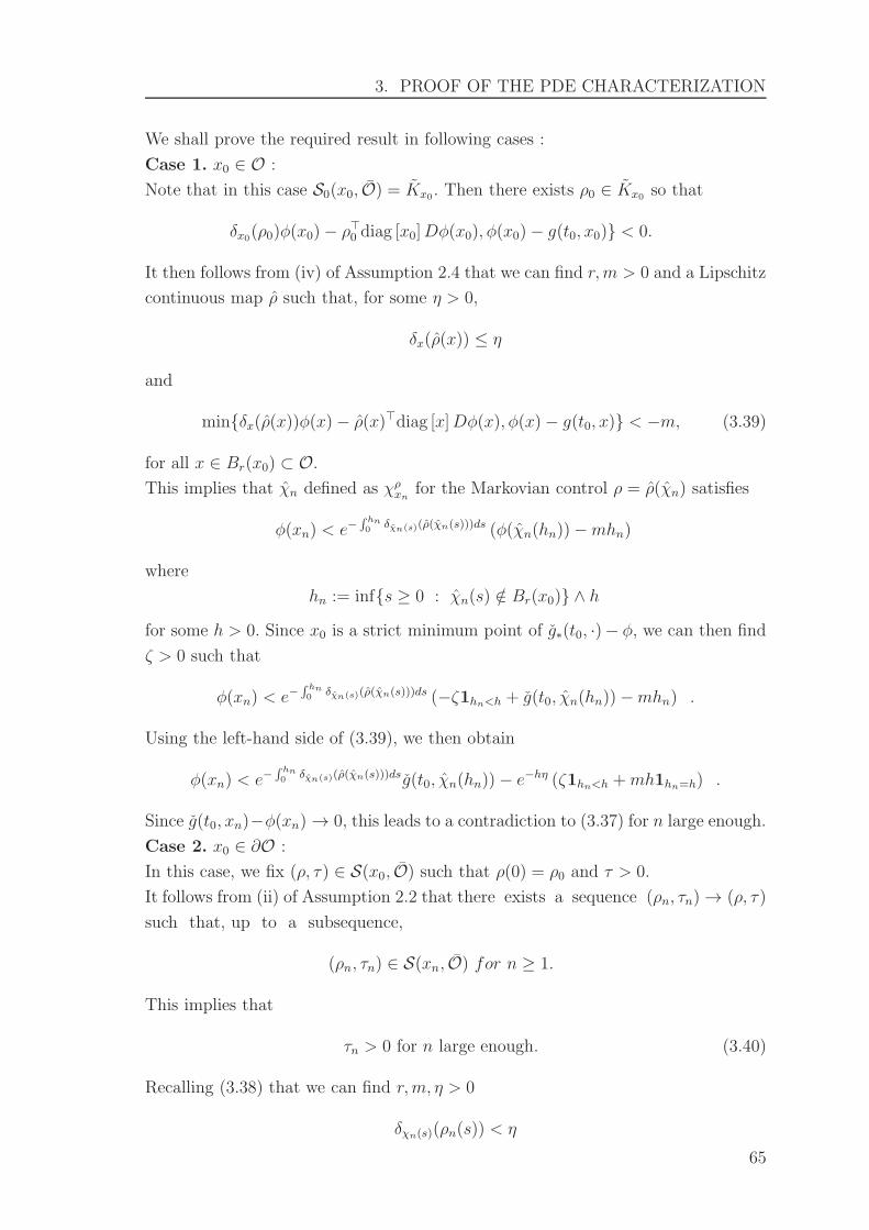
3. PROOF OF THE PDE CHARACTERIZATION
We shall prove the required result in following cases :
Case 1. x0 ∈ O :
Note that in this case S0(x0, O) = Kx0. Then there exists ρ0 ∈ Kx0 so that
δx0(ρ0)φ(x0)− ρ⊤0 diag [x0]Dφ(x0), φ(x0)− g(t0, x0) < 0.
It then follows from (iv) of Assumption 2.4 that we can find r,m > 0 and a Lipschitz
continuous map ρ such that, for some η > 0,
δx(ρ(x)) ≤ η
and
minδx(ρ(x))φ(x)− ρ(x)⊤diag [x]Dφ(x), φ(x)− g(t0, x) < −m, (3.39)
for all x ∈ Br(x0) ⊂ O.
This implies that χn defined as χρxn for the Markovian control ρ = ρ(χn) satisfies
φ(xn) < e−∫ hn0
δχn(s)(ρ(χn(s)))ds (φ(χn(hn))−mhn)
where
hn := infs ≥ 0 : χn(s) /∈ Br(x0) ∧ h
for some h > 0. Since x0 is a strict minimum point of g∗(t0, ·)− φ, we can then find
ζ > 0 such that
φ(xn) < e−∫ hn0 δχn(s)(ρ(χn(s)))ds (−ζ1hn<h + g(t0, χn(hn))−mhn) .
Using the left-hand side of (3.39), we then obtain
φ(xn) < e−∫ hn0 δχn(s)(ρ(χn(s)))dsg(t0, χn(hn))− e−hη (ζ1hn<h +mh1hn=h) .
Since g(t0, xn)−φ(xn) → 0, this leads to a contradiction to (3.37) for n large enough.
Case 2. x0 ∈ ∂O :
In this case, we fix (ρ, τ) ∈ S(x0, O) such that ρ(0) = ρ0 and τ > 0.
It follows from (ii) of Assumption 2.2 that there exists a sequence (ρn, τn) → (ρ, τ)
such that, up to a subsequence,
(ρn, τn) ∈ S(xn, O) for n ≥ 1.
This implies that
τn > 0 for n large enough. (3.40)
Recalling (3.38) that we can find r,m, η > 0
δχn(s)(ρn(s)) < η
65

CHAPITRE 2. APPLICATION TO AMERICAN OPTION PRICING UNDER
CONSTRAINTS
and
−m > min
δχn(s)(ρn(s))φ(χn(s))− ρn(s)
⊤diag [χn(s)]Dφ(χn(s)),
φ(χn(s))− g(t0, χn(s))
,
for s ≤ hn when n is large enough, where
χn := χρnxn and hn := infs ≥ 0 : χn(s) /∈ Br(x0) ∧ τn .
This implies that, for some ζ > 0,
φ(xn)e∫ hn0
δχn(s)(ρn(s))ds
< φ(χn(hn))−mhn
< [g(t0, χn(hn))− ζ ]1hn<τn + [g(t0, χn(hn))−m]1hn≥τn −mhn
which leads to a contradiction of (3.37) since τn > 0.
2.2. We now turn to the subsolution property. Let φ be a non-negative smooth
function and let x0 ∈ O be a strict maximum point of g∗(t0, ·) − φ such that
g∗(t0, x0)−φ(x0) = 0. Let (xn)n be a sequence in O such that g(t0, xn) → g∗(t0, x0).
Assume that
min
inf
ρ∈Kx0
(δx0(ρ)φ(x0)− ρ⊤0 diag [x0]Dφ(x0)
), φ(x0)− g(t0, x0)
> 0 . (3.41)
Since g ≥ 0, this implies that φ > 0 on Br(x0), for some r > 0. Moreover, the fact
that Kx0 is compact implies that, after possibly changing r > 0, we can find ε > 0
such that φ(x) − ε > 0 on Br(x0) and M(x0, φ(x0) − ε,Dφ(x0)) > 0. In view of
Lemma 3.2, this implies that (φ(x0)−ε)−1diag [x0]Dφ(x0) ∈ int(Kx0). It the follows
from Assumption 2.1 that, after possibly changing r > 0, N(x, φ(x) − ε,Dφ(x)) 6=∅ on Br(x0), which, by Lemma 3.2 again, implies that M(x, φ(x) − ε,Dφ(x)) ≥0 on Br(x0). Since δx ≥ cK > 0, recall (iii) of Assumption 2.4, we deduce that
M(x, φ(x), Dφ(x)) ≥ εcK on Br(x0). Using Lemma 3.2, the continuity of g and
(3.41), we finally obtain
min
inf
ρ0∈Kx
(δx(ρ0)φ(x)− ρ⊤0 diag [x]Dφ(x)
), φ(x)− g(t0, x)
≥ m on Br(x0)(3.42)
for some m > 0. Moreover, it follows from Assumption (ii) of Corollary 2.2 that
supδx(ρ0), ρ ∈ Kx ≤ η on Br(x0) (3.43)
for some η > 0. We now consider a sequence (xn)n in O such that g(t0, xn) →g∗(t0, x0). Given (ρ, τ) ∈ S(xn, O), we set hn := infs ≥ 0 : χρxn(s) /∈ Br(x0)66

4. THE EXTENSION TO THE AMERICAN OPTION WITHOUT A BARRIER
for some h > 0. Then, (3.42) and the fact that x0 is a strict maximum point of
g∗(t0, ·)− φ implies that we can find ζ > 0 such that, for all τ ≥ 0,
φ(xn)
≥ e−
∫ hn∧τ0
δχρxn (s)
(ρ(s))ds (φ(χρxn(hn ∧ τ)) +m(hn ∧ τ)
)
≥ e−
∫ hn∧τ0
δχρxn (s)
(ρ(s))ds (g(t0, χ
ρxn(hn))1hn>τ + g(t0, χ
ρxn(τ))1τ≤hn + ζ ∧m ∧ (mh)
).
Since φ(xn) − g(t0, xn) → 0, the above inequality combined with (3.43) leads to a
contradiction to (3.37) for n large enough, by arbitrariness of τ and ρ. 2
We can now conclude the proof of Corollary 2.2.
Proof of Corollary 2.2 The subsolution property follows from Theorem 2.2 since
g ≥ g. As for the supersolution property, we note that Theorem 2.2 implies that,
for fixed t0 ∈ [0, T ], v∗(t0, ·) is a supersolution of minϕ − g(t0, ·),Mdϕ ≥ 0. It
thus follows from Lemma 3.9 that v∗ ≥ g. The supersolution property then follows.
To conclude, we note that the comparison result of Proposition 5.1 obviously still
holds if we replace g by g since g is continuous with respect to its first variable by
assumption, and with respect to its second one by Lemma 3.10. 2
Remark 3.2 Note that the supersolution property v∗ ≥ g(T, ·) could be proved as
a direct consequence of Lemma 3.4. However, above proof is provide to focus on
studying g(t0, ·) is continuous on O and is the unique viscosity solution of (3.34)-
(3.35) and without required the viscosity solution of v.
4 The extension to the American option without
a barrier
In this section, we explain how the obstacle version of geometric dynamic pro-
gramming principle in Theorem 2.1 of Chapter 1 can be used to relate the super-
hedging price of an American option under constraints without a barrier, i.e O = Rd,
which has been further studied by [15]. The super-hedging price is thus defined as
v(t, x) := infy ∈ R+ : ∃ π ∈ A s.t Y π
t,x,y(τ) ≥ g(τ,Xt,x(τ)) ∀ τ ∈ T[t,T ]
. (4.1)
Observe that v(t, x) coincides with the lower bound of the set y ∈ R+ : (x, y) ∈V (t) where
V (t) := (x, y) ∈ (0,∞)d × R+ : ∃ π ∈ A s.t. Zπt,x,y(τ) ∈ G(τ) ∀ τ ∈ T[t,T ],
It follows from the obstacle geometric dynamic programming principle of Theorem
2.1 that
67

CHAPITRE 2. APPLICATION TO AMERICAN OPTION PRICING UNDER
CONSTRAINTS
Corollary 4.1 Fix (t, x, y) ∈ [0, T ]× (0,∞)d × R+.
(DP1). If y > (t, x), then there exists π ∈ A such that
Y πt,x,y(θ) ≥ v(θ,Xt,x(θ)) for all θ ∈ T[t,T ] .
(DP2) If y < v(t, x), then ∃ τ ∈ T[t,T ] such that
P[Y πt,x,y(θ ∧ τ) > v(θ,Xt,x,y(θ))1θ<τ + g(τ,Xt,x,y(τ))1θ≥τ
]< 1
for all θ ∈ T[t,T ] and π ∈ A.
We observer that S0(x,Rd) = Kx and therefore Mdv(t, x) coincides to Mv(t, x)
for all (t, x) ∈ [0, T ] × Rd, recall Remark 2.6. This allows us to provide a PDE
characterization of v without worrying about the operator Md.
Theorem 4.1 Let the conditions of Theorem 2.3 hold. Then, v is a discontinuous
viscosity solution of
minHϕ, Mϕ = 0 on [0, T )× (0,∞)d,
min ϕ(T, x)− g(T, x) , Mϕ(T, x) = 0 on (0,∞)d(4.2)
and satisfies the boundary condition
v∗(T, x) = v∗(T, x) = g(T, x) on (0,∞)d. (4.3)
Moreover, it is the unique viscosity solution of (4.2)-(4.3) in the class of non-negative
functions satisfying
|v(t, x)| ≤ C (1 + xγ) ∀(t, x) ∈ [0, T ]× (0,∞)d.
In the case where σ is invertible, the above discussion already shows that g = g.
If moreover µ and σ are constant, we can actually interpret the super-hedging price
as the price of an American option with payoff g, without taking the portfolio
constraints into account. This phenomenon was already observed for plain vanilla
or barrier european options, see e.g. [9] and [13]. It comes from the fact that, when
the parameters are constant, the gradient constraint imposed at T by the termi-
nal condition v(T, ·) = g propagates into the domain. It is therefore automatically
satisfied and we retrieve the result of Corollary 1 in [13].
Corollary 4.2 Let the conditions of Theorem 2.3 hold. Assume further that µ and
σ are constant and that σ is invertible. Then, g = g and
v(t, x) = supτ∈Tt,x
EQ [g(τ,Xt,x(τ))] (4.4)
where Q ∼ P is defined by
dQ
dP:= e−
12|σ−1µ|2T+(σ−1µ)⊤WT .
68

4. THE EXTENSION TO THE AMERICAN OPTION WITHOUT A BARRIER
Remark 4.1 Since σ is constant and invertible, the condition that µ is constant
could be relaxed, under mild assumptions, by performing a suitable initial change
of measure.
Proof of Corollary 4.2. The fact that g = g follows from the discussion at the
beginning of Section 2.4. Note that the continuity of g implies that g is continuous
too. Also observe that the fact that σ is invertible implies that, for a smooth function
ϕ,
supπ∈Nϕ(t,x)
(π⊤µ(x)ϕ(t, x)−Lϕ(t, x)
)= −∂tϕ− 1
2Trace
[diag [x] σσ⊤diag [x]D2ϕ
].(4.5)
Let us now observe that the map w defined on [0, T ]× (0,∞)d by
w(t, x) := supτ∈T[t,T ]
EQ [g(τ,Xt,x(τ))]
is a viscosity solution on [0, T )× (0,∞)d of
min
−∂tϕ− 1
2Trace
[diag [x] σσ⊤diag [x]D2ϕ
], ϕ− g
= 0 . (4.6)
In particular, it is a subsolution of (4.2), recall (4.5). We next deduce from the
definition of g that, for all ρ ∈ Rd,
w(t, xeρ) = supτ∈T[t,T ]
EQ [g(τ,Xt,x(τ)eρ)] ≤ sup
τ∈T[t,T ]
EQ[eδ(ρ)g(τ,Xt,x(τ))
]= eδ(ρ)w(t, x) .
It follows that w(t, x) ≥ e−δ(ρ)w(t, xeρ) for all ρ ∈ Rd which implies that w is a
viscosity supersolution of Mϕ = 0. Hence, w is a supersolution of (4.2), recall (4.5).
Finally, (3.36) and standard estimates show that w satisfy the growth condition
(2.16). It thus follows from Corollary 2.2 that v∗ = v∗ = w. 2
69

CHAPITRE 2. APPLICATION TO AMERICAN OPTION PRICING UNDER
CONSTRAINTS
70

Deuxieme partie
The stochastic target problems
with multiple constraints in
probability
71


Chapitre 3
A stochastic target approach for
P&L matching problems
1 Introduction
Option pricing (in incomplete financial markets or markets with frictions) and
optimal management decisions have to be based on some risk criterion or, more
generally, on some choice of preferences. In the academic literature, one usually
models the attitude of the financial agents toward risk in terms of an utility or loss
function. However, practitioners have in general no idea of “their utility function”.
Even the choice of a loss function is somehow problematic. On the other hand, they
have a rough idea on the type of P&L they can afford, and indeed have as a target.
This is the case for traders, for hedge-fund managers,...
The aim of this chapter is to provide a direct PDE characterization of the minimal
initial endowment required so that the terminal wealth of a financial agent (possibly
diminished by the payoff of a random claim) can match a set of constraints in
probability. In practice, this set of constraints has to be viewed as a rough description
of a targeted P&L distribution.
To be more precise, let us consider the problem of a trader who would like to
hedge a European claim of the form g(Xt,x(T )), where Xt,x models the evolution of
some risky assets, assuming that their value is x at time t. The aim of the trader
is to find an initial endowment y and a hedging strategy ν such that the terminal
value of his hedging portfolio Y νt,x,y(T ) diminished by the liquidation value of the
claim g(Xt,x(T )) matches an a-priori distribution of the form
P[Y νt,x,y(T )− g(Xt,x(T )) ≥ −γi
]≥ pi , i ≤ κ ,
where γκ ≥ · · · ≥ γ2 ≥ γ1 ≥ 0, for some κ ≥ 1. The minimal initial endowment
73

CHAPITRE 3. A STOCHASTIC TARGET APPROACH FOR P&L MATCHING
PROBLEMS
required to achieve the above constraints is given by :
v(t, x, p)
:= infy : ∃ ν s.t. Y νt,x,y(T ) ≥ ℓ,P
[Y νt,x,y(T )− g(Xt,x(T )) ≥ −γi
]≥ pi ∀ i ≤ κ,
where we used the notation p := (p1, . . . , pκ) and ℓ ∈ R is a given lower bound that
is imposed in order to avoid that the wealth goes too negative, even if it is with
small probability.
In the case κ = 1, such a problem is referred to as the “quantile hedging pro-
blem”. It has been widely studied by Follmer and Leukert [23] who provided an
explicit description of the optimal terminal wealth Y νt,x,y(T ) in the case where the
underlying financial market is complete. This result is derived from a clever use of the
Neyman-Pearson Lemma in mathematical statistics and applies to non-Markovian
frameworks. A direct approach, based on the notion of stochastic target problems,
has then been proposed by Bouchard, Elie and Touzi [12]. It allows to provide a
PDE characterization of the pricing function v, even in incomplete markets or in
cases where the stock price process Xt,x can be influenced by the trading strategy
ν, see e.g. [10]. The problem (0.8) is a generalization of this work to the case of
multiple constraints in probability.
As in Bouchard, Elie and Touzi [12], the first step consists in rewriting the sto-
chastic target problem with multiple constraints in probability (0.8) as a stochastic
target problem in the P−a.s. sense. This is achieved by introducing a suitable family
of d-dimensional bounded martingales P αt,p, α and by re-writing v as
v(t, x, p)
= infy : ∃ (ν, α) s.t Y νt,x,y(T ) ≥ ℓ,min
i≤κ
(∆i(Xt,x(T ), Y
νt,x,y(T ))− P α,i
t,p (T ))≥ 0 ,
where ∆i(x, y) := 1y−g(x)≥−γi and P α,it,p denotes the i-th component of P α
t,p. As in
[12], “at the optimum” each process P α,it,p has to be interpreted as the martingale
coming from the martingale representation of 1Y νt,x,y(T )−g(Xt,x(T ))≥−γi. The above re-
duction allows to appeal to the Geometric dynamic programming principle (GDPP)
of Soner and Touzi [46], which leads to the PDE characterization stated in Theorem
2.1 below, with suitable boundary conditions.
In this chapter, we focus on the case where the market is complete but the
amount of money that can be invested in the risky assets is bounded. The incomplete
market case could be discussed by following the lines of the paper, but will add extra
complexity. Since the proofs below are already complex, we decided to restrict to
the complete market case. The fact that the amount of money that can be invested
in the risky assets is bounded could also be relaxed. It does not really simplifies the
arguments. On the other hand, it is well-known that quantile hedging type strategies
can lead to the explosion of the number of risky asset to hold in the portfolio near
74
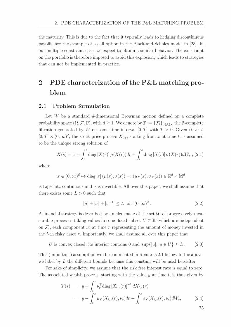
2. PDE CHARACTERIZATION OF THE P&L MATCHING PROBLEM
the maturity. This is due to the fact that it typically leads to hedging discontinuous
payoffs, see the example of a call option in the Black-and-Scholes model in [23]. In
our multiple constraint case, we expect to obtain a similar behavior. The constraint
on the portfolio is therefore imposed to avoid this explosion, which leads to strategies
that can not be implemented in practice.
2 PDE characterization of the P&L matching pro-
blem
2.1 Problem formulation
Let W be a standard d-dimensional Brownian motion defined on a complete
probability space (Ω,F ,P), with d ≥ 1. We denote by F := Ft0≤t≤T the P-complete
filtration generated by W on some time interval [0, T ] with T > 0. Given (t, x) ∈[0, T ]× (0,∞)d, the stock price process Xt,x, starting from x at time t, is assumed
to be the unique strong solution of
X(s) = x+
∫ s
t
diag [X(r)]µ(X(r))dr +
∫ s
t
diag [X(r)]σ(X(r))dWr , (2.1)
where
x ∈ (0,∞)d 7→ diag [x] (µ(x), σ(x)) =: (µX(x), σX(x)) ∈ Rd ×Md
is Lipschitz continuous and σ is invertible. All over this paper, we shall assume that
there exists some L > 0 such that
|µ|+ |σ|+ |σ−1| ≤ L on (0,∞)d . (2.2)
A financial strategy is described by an element ν of the set U t of progressively mea-
surable processes taking values in some fixed subset U ⊂ Rd which are independent
on Ft, each component νir at time r representing the amount of money invested in
the i-th risky asset r. Importantly, we shall assume all over this paper that
U is convex closed, its interior contains 0 and sup|u|, u ∈ U ≤ L . (2.3)
This (important) assumption will be commented in Remarks 2.1 below. In the above,
we label by L the different bounds because this constant will be used hereafter.
For sake of simplicity, we assume that the risk free interest rate is equal to zero.
The associated wealth process, starting with the value y at time t, is thus given by
Y (s) = y +
∫ s
t
ν⊤r diag [Xt,x(r)]−1 dXt,x(r)
= y +
∫ s
t
µY (Xt,x(r), νr)dr +
∫ s
t
σY (Xt,x(r), νr)dWr, (2.4)
75

CHAPITRE 3. A STOCHASTIC TARGET APPROACH FOR P&L MATCHING
PROBLEMS
where
µY (x, u) := u⊤µ(x) and σY (x, u) := u⊤σ(x) , (x, u) ∈ Rd+ × U .
The aim of the trader is to hedge an European option of payoff g(Xt,x(T )) at time
T , where
g : (0,∞)d 7→ R is Lipschitz continuous. (2.5)
Here, the price is chosen so that the net wealth Y νt,x,y(T ) − g(Xt,x(T )) satisfies a
P&L constraint. Namely, given a collection of thresholds γ := (γi)i≤κ ∈ Rκ and of
probabilities (pi)i≤κ ∈ [0, 1]κ, for some κ ≥ 1, the price of the option is defined as
the minimal initial wealth y such that there exists a strategy ν ∈ U satisfying
P[Y νt,x,y(T ) ≥ gi(Xt,x(T ))] ≥ pi for all i ∈ 1, . . . , κ =: K , (2.6)
where
gi := g − γi , i ∈ K . (2.7)
Obviously, we can assume without loss of generality that
0 ≤ γ1 ≤ γ2 ≤ · · · ≤ γκ . (2.8)
This means that the net hedging loss should not exceed −γi with probability more
than pi. This coincides with a constraint on the distribution of the P&L of the
trader, in the sense that it should match the constraints imposed by the discrete
histogram associated to (γ, p). In order to avoid that the wealth process goes too
negative, even with small probability, we further impose that Y νt,x,y(T ) ≥ ℓ for some
ℓ ∈ R−. The price is then defined, for (t, x, p) ∈ [0, T ]× (0,∞)d × [0, 1]κ, as :
v(t, x, p) (2.9)
:= infy ≥ ℓ : ∃ν ∈ U t s.t Y νt,x,y(T ) ≥ ℓ, P[Y ν
t,x,y(T ) ≥ gi(Xt,x(T ))] ≥ pi ∀i ∈ K .
Note that, after possibly changing g and γ, one can always reduce to the case
where
g1 ≥ g2 ≥ · · · ≥ gκ ≥ ℓ . (2.10)
We further assume that g is bounded from above and that gκ > ℓ uniformly, which,
after possibly changing the constant L can be written as
ℓ+ L−1 ≤ gκ ≤ g ≤ L . (2.11)
76
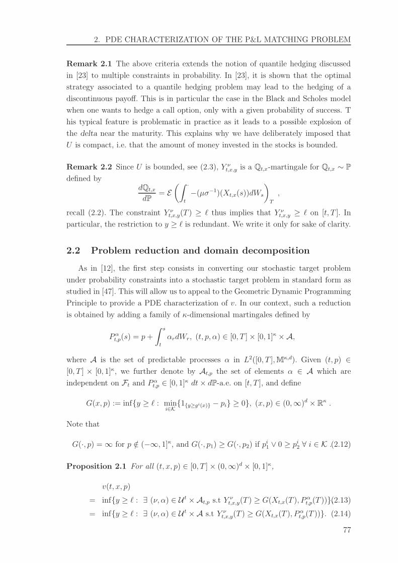
2. PDE CHARACTERIZATION OF THE P&L MATCHING PROBLEM
Remark 2.1 The above criteria extends the notion of quantile hedging discussed
in [23] to multiple constraints in probability. In [23], it is shown that the optimal
strategy associated to a quantile hedging problem may lead to the hedging of a
discontinuous payoff. This is in particular the case in the Black and Scholes model
when one wants to hedge a call option, only with a given probability of success. T
his typical feature is problematic in practice as it leads to a possible explosion of
the delta near the maturity. This explains why we have deliberately imposed that
U is compact, i.e. that the amount of money invested in the stocks is bounded.
Remark 2.2 Since U is bounded, see (2.3), Y νt,x,y is a Qt,x-martingale for Qt,x ∼ P
defined bydQt,x
dP= E
(∫ ·
t
−(µσ−1)(Xt,x(s))dWs
)
T
,
recall (2.2). The constraint Y νt,x,y(T ) ≥ ℓ thus implies that Y ν
t,x,y ≥ ℓ on [t, T ]. In
particular, the restriction to y ≥ ℓ is redundant. We write it only for sake of clarity.
2.2 Problem reduction and domain decomposition
As in [12], the first step consists in converting our stochastic target problem
under probability constraints into a stochastic target problem in standard form as
studied in [47]. This will allow us to appeal to the Geometric Dynamic Programming
Principle to provide a PDE characterization of v. In our context, such a reduction
is obtained by adding a family of κ-dimensional martingales defined by
P αt,p(s) = p+
∫ s
t
αrdWr, (t, p, α) ∈ [0, T ]× [0, 1]κ ×A,
where A is the set of predictable processes α in L2([0, T ],Mκ,d). Given (t, p) ∈[0, T ] × [0, 1]κ, we further denote by At,p the set of elements α ∈ A which are
independent on Ft and Pαt,p ∈ [0, 1]κ dt× dP-a.e. on [t, T ], and define
G(x, p) := infy ≥ ℓ : mini∈K
1y≥gi(x) − pi ≥ 0, (x, p) ∈ (0,∞)d × Rκ .
Note that
G(·, p) = ∞ for p /∈ (−∞, 1]κ, and G(·, p1) ≥ G(·, p2) if pi1 ∨ 0 ≥ pi2 ∀ i ∈ K .(2.12)
Proposition 2.1 For all (t, x, p) ∈ [0, T ]× (0,∞)d × [0, 1]κ,
v(t, x, p)
= infy ≥ ℓ : ∃ (ν, α) ∈ U t ×At,p s.t Y νt,x,y(T ) ≥ G(Xt,x(T ), P
αt,p(T )),(2.13)
= infy ≥ ℓ : ∃ (ν, α) ∈ U t ×A s.t Y νt,x,y(T ) ≥ G(Xt,x(T ), P
αt,p(T )). (2.14)
77

CHAPITRE 3. A STOCHASTIC TARGET APPROACH FOR P&L MATCHING
PROBLEMS
Proof. The proof follows from the same arguments as in [12]. We provide it for
completeness. We fix (t, x, p) ∈ [0, T ]× (0,∞)d× [0, 1]κ, set v := v(t, x, p) for ease of
notations, and denote by w1 and w2 the right-hand side of (2.13) and (2.14) respecti-
vely. The fact that w1 ≥ w2 is obvious. Conversely, if Yνt,x,y(T ) ≥ G(Xt,x(T ), P
αt,p(T ))
for some (ν, α) ∈ U t × A, then (2.12) implies that P α,it,p (T ) ≤ 1 for all i ∈ K. Since
P αt,p is a martingale, it takes values in (−∞, 1]κ on [t, T ]. Moreover, we can find
α ∈ A such that P α,it,p (T ) = 0 on Ai := min[t,T ] P
α,it,p ≤ 0 and P α,i
t,p (T ) = P α,it,p (T )
on Aci for i ∈ K. It follows from the above discussion and the martingale property
of P αt,p that it takes values in [0, 1]κ on [t, T ], so that α ∈ At,p. Since P
α,it,p (T ) ≤
P α,it,p (T ) ∨ 0, the inequality Y ν
t,x,y(T ) ≥ G(Xt,x(T ), Pαt,p(T )) together with (2.12) im-
ply that Y νt,x,y(T ) ≥ G(Xt,x(T ), P
αt,p(T )). This shows that w2 ≥ w1, so that w2 = w1.
It remains to show that v = w2. The inequality w2 ≥ v is an immediate consequence
of the martingale property of P αt,p. On the other hand, for y > v, we can find ν ∈ U
such that pi := P[Y νt,x,y(T ) ≥ gi(Xt,x(T ))] ≥ pi for all i ∈ K. Set p := (pi)i∈K.
Then, the martingale representation theorem implies that we can find α ∈ A such
that P α,it,p (T ) = 1Y ν
t,x,y(T )≥gi(Xt,x(T )) for each i ∈ K. We conclude by observing that
P α,it,p (T ) ≥ P α,i
t,p (T ) for each i ∈ K. 2
Remark 2.3 As in [12], the new controlled process P αt,p should be interpreted as
the martingale with components given by (P[Y νt,x,y(T ) ≥ gi(Xt,x(T )) | Fs])s∈[t,T ], at
least when the controls ν and α are optimal. This is rather transparent in the above
proof. The fact that we can restrict to the set of controls At,p is therefore clear since
a conditional probability should take values in [0, 1].
Remark 2.4 Note that α ∈ At,p implies that αi· ≡ 0 for all i ∈ K such that
pi ∈ 0, 1, since P αt,p is a martingale.
The representation (2.14) coincides with a stochastic target problem in standard
form but with unbounded controls as studied in [12], unbounded referring to the
fact that α can not be bounded a-priori since it comes from the martingale repre-
sentation theorem. In particular, a PDE characterization of the value function v in
the parabolic interior of the domain
D := [0, T )× (0,∞)d × (0, 1)κ
follows from the general results of [12]. The main difference comes from the fact that
the constraints P α,i ∈ [0, 1] introduce boundary conditions that have to be discussed
separately. In order to deal with these boundary conditions, we first divide the
closure of the domain D into different regions corresponding to its parabolic interior
D and the different boundaries associated to the level of conditional probabilities.
Namely, given
Pκ := (I, J) ∈ K2 : I ∩ J = ∅ and I ∪ J ⊂ K,78

2. PDE CHARACTERIZATION OF THE P&L MATCHING PROBLEM
we set, for (I, J) ∈ Pκ,
DIJ := [0, T )× (0,∞)d × BIJ , (2.15)
where
BIJ := p ∈ [0, 1]κ : pi = 0 for i ∈ I, pj = 1 for j ∈ J, and 0 < pl < 1 for l /∈ I ∪ J .
Then,
[0, T )× (0,∞)d × [0, 1]κ = ∪(I,J)∈PκDIJ .
The interpretation of the partition is the following. For (t, x, p) ∈ D, any pi takes
values in (0, 1) so that P α,it,p is not constrained locally at time t by the state constraints
which appears in (2.13), namely P α,it,p ∈ [0, 1]. This means that the control αi· can
be chosen arbitrarily, at least locally around the initial time t. When (t, x, p) ∈ DIJ
with I ∪ J 6= ∅, then there is at least one i ≤ κ such that pi = 0 or pi = 1. In this
case the state constraints P α,it,p ∈ [0, 1] on [t, T ] imposes to choose αi· = 0 on [t, T ],
see Remark 2.4. Hence, letting πIJ be the operator defined by
p ∈ [0, 1]κ 7→ πIJ(p) = (pi1i/∈I∪J + 1i∈J)i∈K (2.16)
for (I, J) ∈ Pκ, we have
v = vIJ := v(·, πIJ(·)) on DIJ , (2.17)
where, for (t, x, p) ∈ D,
vIJ(t, x, p) (2.18)
= infy ≥ ℓ : Y νt,x,y(T ) ≥ G(Xt,x(T ), P
αt,πIJ(p)
(T )) for some (ν, α) ∈ U t ×AIJt,πIJ(p)
with
AIJt,πIJ (p)
:=α ∈ At,p : α
i· = 0 for all i ∈ I ∪ J,
recall Remark 2.4.
In the rest of the paper, we shall write (I, J) ∈ Pkκ when (I, J) ∈ Pκ and
|I| + |J | = k, k ≤ κ. We shall also use the notations (I ′, J ′) ⊃ (I, J) when I ′ ⊃ I
and J ′ ⊃ J . If in addition, (I ′, J ′) 6= (I, J), then we will write (I ′, J ′) ) (I, J).
Remark 2.5 It is clear that v and each vIJ , (I, J) ∈ Pκ, are non-decreasing with
respect to their p-parameter. In particular, vIJ ′ ≥ vIJ ≥ vI′J for (I ′, J ′) ⊃ (I, J).
Remark 2.6 Since gi ≥ gj for i ≤ j, it would be natural to restrict to the case where
pi ≤ pj for i ≤ j. From the PDE point of view, this would lead to the introduction
of boundary conditions on the planes for which pi = pj for some i 6= j. Since this
restriction does not appear to be necessary in our approach, we deliberately do not
use this formulation. From the pure numerical point of view, one could however use
the fact that v(·, p) = v(·, p) where p is defined by pj = maxi≤j pj for i ≤ κ.
79

CHAPITRE 3. A STOCHASTIC TARGET APPROACH FOR P&L MATCHING
PROBLEMS
Remark 2.7 Note that, as defined above on DIJ , the function vIJ depends on its
p-parameters only through the components (pl)l /∈I∪J . However, for ease of notations,
we shall always use the notation vIJ(·, p) instead of a more transparent notation such
as vIJ(t, x, (pl)l /∈I∪J). Similarly, a test function on DIJ depends on the p-parameter
only through (pl)l /∈I∪J .
Remark 2.8 Note that, for any J ⊂ K,
vJcJ = infy ≥ ℓ : Y νt,x,y(T ) ≥ gJ(Xt,x(T )) for some ν ∈ U t,
where
gJ := maxj∈J
gj ∨ ℓ (2.19)
coincides with the super-hedging price of the payoff gJ(Xt,x(T )), while
vK∅ = infy ≥ ℓ : ∃ ν ∈ U t s.t 1Y νt,x,y(T )≥maxi≤κ gi(Xt,x(T )) ≥ 0 and Y ν
t,x,y(T ) ≥ ℓ = ℓ .
2.3 PDE characterization
As already mentioned, stochastic target problems of the form (2.18) have been
studied in [12] which provides a PDE characterization of each value function vIJ on
DIJ . In order to state it, we first need to introduce some additional notations. For
ease of notations, we set
µX,P :=
(µX
0κ
)and σX,P (·, a) :=
(σX
a
)for a ∈ Mκ,d ,
where 0κ := (0, . . . , 0) ∈ Rκ.
Given (I, J) ∈ Pκ and ε > 0, we then define
F ǫIJ := sup
(u,a)∈NǫIJ
Lu,a,
where, for (u, a) ∈ U ×Mκ,d and θ := (x, q, Q) ∈ Θ := (0,∞)d × Rd+κ ×Md+κ,d+κ,
Lu,a(θ) := µY (x, u)− µX,P (x)⊤q − 1
2Trace
[(σX,Pσ
⊤X,P )(x, a)Q
],
and
N ǫIJ := (u, a) ∈ U × AIJ : |N u,a| ≤ ǫ
with
N u,a(x, q) := σY (x, u)−q⊤σX,P (x, a) and AIJ := a ∈ Mκ,d : ak· = 0 for k ∈ I∪J .
The main result of [12] states that vIJ is a discontinuous viscosity solution of the
PDE
minϕ− ℓ , −∂tϕ+ F 0IJ(·, Dϕ,D2ϕ) = 0 on DIJ ,
80

2. PDE CHARACTERIZATION OF THE P&L MATCHING PROBLEM
where, for a smooth function ϕ : (t, x, p) ∈ [0, T ]×Rd ×Rκ, Dϕ and D2ϕ stand for
the gradient and the Hessian matrix with respect to (x, p), and ∂tϕ stands for the
time derivative. The label “discontinuous viscosity solution” means that it has be
stated in terms of the upper- and lower-semicontinuous envelopes of v, see Definition
2.2 below, and that we need to relax the operator F 0IJ , which may not be continuous,
by considering the upper- and lower-semicontinuous envelopes F ∗IJ and FIJ∗
F ∗IJ(θ) := lim sup
(θ′, ε′) → (θ, 0)
(θ′, ε′) ∈ Θ × R+
F ε′
IJ(θ′) and FIJ∗(θ) := lim inf
(θ′, ε′) → (θ, 0)
(θ′, ε′) ∈ Θ × R+
F ε′
IJ(θ′) .
This leads to a system, hereafter called (S), of PDEs, each stated on a sub-
domain DIJ , with appropriate boundary conditions, see Theorem 2.2 and Corollary
2.1 below.
Before defining precisely what we mean by a solution of (S), we need to introduce
an extra technical object to which we will appeal when we define the notion of
subsolution.
Definition 2.1 Given (I, J) ∈ Pκ and (t, x, p) ∈ DIJ , we denote by CIJ (t, x, p) theset of C1,2 functions ϕ with the following property : for all ε > 0, all open set B such
that (x,Dϕ(t, x, p)) ∈ B and N0IJ 6= ∅ on B, and all (u, a) ∈ N0
IJ(x,Dϕ(t, x, p)),
there exists an open neighborhood B′ of (x,Dϕ(t, x, p)) and a locally Lipschitz map
(u, a) such that |(u, a)(x,Dϕ(t, x, p))− (u, a)| ≤ ε and (u, a) ∈ N0IJ on B′.
Remark 2.9 Fix (I, J) ∈ Pκ such that there exists i ∈ K \ (I ∪ J). Let ϕ be a
smooth function such that Dpiϕ 6= 0 on a neighborhood of (t, x, p) ∈ D. Then,
(u, a) ∈ N0IJ(x,Dϕ(t, x, p)) is equivalent to
ai· =
σY (x, u)−Dxϕ(t, x, p)
⊤σX(x)−∑
j /∈I∪J∪i
aj·Dpjϕ(t, x, p)
/Dpiϕ(t, x, p).
SinceDpiϕ 6= 0 on a neighborhood of (t, x, p), this readily implies that ϕ ∈ CIJ(t, x, p).
A viscosity solution of (S) is then defined as follows.
Definition 2.2 (i) Given a locally bounded map V defined on D and (I, J) ∈ Pκ,we define VIJ := V (·, πIJ(·)) and
V ∗IJ(t, x, p) := lim sup
(t′, x′, p′) → (t, x, p)
(t′, x′, p′) ∈ DIJ
VIJ(t′, x′, p′)
and
VIJ∗(t, x, p) := lim inf(t′, x′, p′) → (t, x, p)
(t′, x′, p′) ∈ DIJ
VIJ(t′, x′, p′) ,
81

CHAPITRE 3. A STOCHASTIC TARGET APPROACH FOR P&L MATCHING
PROBLEMS
for (t, x, p) ∈ DIJ .
(ii) We say that V is a discontinuous viscosity supersolution of (S) if VIJ∗ is a
viscosity supersolution of
minϕ− ℓ , −∂tϕ+ F ∗
IJ(·, Dϕ,D2ϕ)= 0 on DIJ , (2.20)
for each (I, J) ∈ Pκ.
(iii) We say that V is a discontinuous viscosity subsolution of (S) if V ∗IJ is a viscosity
subsolution of
minϕ− ℓ , −∂tϕ+ FIJ∗(·, Dϕ,D2ϕ)
= 0 if ϕ ∈ CIJ , on DIJ , (2.21)
for each (I, J) ∈ Pκ.
(iv) We say that V is a discontinuous viscosity solution of (S) if it is both a discon-
tinuous super- and subsolution of (S).
We can now state our first result which is a direct Corollary of Theorem 2.1 in
[12].
Theorem 2.1 The function v is a discontinuous viscosity solution of (S).
Proof. The above result is an immediate consequence of Theorem 2.1 in [12]. Note
that we replaced their condition Assumption 2.1 by the condition ϕ ∈ CIJ , which is
equivalent, in the statement of the subsolution property, see Remark 2.9. 2
Remark 2.10 Fix (I, J) ∈ Pκ such that I∪J = K. Then, (u, a) ∈ N εIJ(x,Dϕ(t, x, p))
implies that
|u⊤σ(x)−Dxϕ(t, x, p)⊤diag [x] σ(x)| ≤ ε .
Since u ∈ U and σ(x) is invertible by assumption, one easily checks that (2.20)
implies
diag [x]Dxϕ(t, x, p) ∈ U , (2.22)
recall the usual convention sup ∅ = −∞. This is the classical gradient constraint
that appears in super-hedging problems with constraints on the strategy, see e.g.
[20], where it is written in terms of proportions of the wealth invested in the risky
assets.
82

2. PDE CHARACTERIZATION OF THE P&L MATCHING PROBLEM
Remark 2.11 Let ϕ be a smooth function. If Dpiϕ(t, x, p) = 0 for i /∈ I ∪ J , thenN εIJ(x,Dϕ(t, x, p)) takes the form Uε × Mκ,d for some Uε ⊂ U , ε > 0. Thus the
optimization over a ∈ Mκ,d in the definition of F εIJ is performed over an unbounded
set. On the other hand, if Dpiϕ(t, x, p) > 0 for i /∈ I ∪ J , t hen the same arguments
as in Remark 2.9 imply that at least one line of a is given by the other ones. In
particular, for |I| + |J | = κ − 1, the sequence of sets (N εIJ(x,Dϕ(t, x, p)))0≤ε≤1 is
contained in a compact subset of U ×Mκ,d. This implies that F ∗IJ 6= FIJ∗ in general.
As already mentioned the main difficulty comes from the boundary conditions.
We first state the space boundary condition in the p-variable, whose proof is provided
later in Section 3.
Theorem 2.2 Fix (I, J), (I ′, J ′) ∈ Pκ such that (I ′, J ′) ⊃ (I, J), we have
(i) vIJ∗ is viscosity supersolution of
minϕ− ℓ , −∂tϕ+ F ∗
IJ ′(·, Dϕ,D2ϕ)= 0 on DIJ ′,
(ii) v∗IJ(t, x, p) ≤ v∗I′J ′(t, x, p), for (t, x, p) ∈ DIJ ∩ [0, T ]× (0,∞)d ×BI′J ′.
We now discuss the boundary condition as t approaches T .
In the case where I ∪ J = K with |J | > 0, the map vIJ coincides with the super-
hedging problem associated to the payoff gJ as defined in (2.19), recall Remark 2.8.
One could therefore expect that vIJ(T−, ·) = gJ . However, as usual, see e.g. [20],
the terminal condition for vIJ is not the natural one since the gradient constraint
that appears implicitly in (2.21), see Remark 2.10, should propagate up to the time
boundary. The natural boundary condition should be given by the smallest function
φ above gJ that satisfies the associated gradient constraint diag [x]Dxφ ∈ U . This
leads to the introduction of the “face-lifted” version of gJ defined by :
gJ(x) := supζ∈Rd
[gJ(xeζ)− δU(ζ)] , (2.23)
where
δU (ζ) := supu∈U
u⊤ζ , ζ ∈ Rd (2.24)
is the support function of the convex closed set U and xeζ = (xieζi)i≤d.
When I ∪ J 6= K, the above mentioned gradient constraint does not appear
anymore in (2.21), see e.g. Remark 2.9, and the terminal boundary condition can
83

CHAPITRE 3. A STOCHASTIC TARGET APPROACH FOR P&L MATCHING
PROBLEMS
be naturally stated in terms of
G(x, p) := infy ≥ ℓ : y ≥ gi(x)10<pi<1 + gi(x)1pi=1, for all i ∈ K= max
i∈K
(ℓ1pi=0 + gi(x)10<pi<1 + gi(x)1pi=1
). (2.25)
Corollary 2.1 v∗(T, ·) ≥ G∗ and v∗(T, ·) ≤ G∗ on (0,∞)d × [0, 1]κ.
Proof. It is a consequence of Proposition 1.2 and Theorem 1.1 in the next chapter.
2
Remark 2.12 In the case of κ = 1 and g1 ≥ ℓ = 0, it is shown in [23] and [12]
that the terminal condition should be face-lifted with respect to the p-variable when
the set U in which controls take values is Rd. This follows from the convexity of the
value function in its p-variable. Namely, the terminal condition as t → T is then
given by p1g1. Corollary 2.1 shows that it is no more the case when we restrict to a
compact set U .
Remark 2.13 Combining Theorem 2.1, Theorem 2.2 and Corollary 2.1 provides
a PDE characterization of the value function v. However, the following should be
noted :
1. It is clear that G∗ < G∗ for some p ∈ ∂[0, 1]κ.
2. The boundary conditions induced by Theorem 2.2 may not lead to vIJ∗ ≥ v∗IJon the boundary in the p-variable.
3. The operator FIJ in (2.20) and (2.21) is in general discontinuous when I ∪J 6=K, see Remark 2.11 above.
This prevents us from proving a general comparison result for super- and sub-
solutions of (S). We are therefore neither able to prove that v is the unique solution
of (S) in a suitable class, nor to prove the convergence of standard finite difference
numerical schemes. In order to surround this difficulty, we shall introduce in the next
chapter a sequence of convergent approximating problems which are more regular
and for which convergent schemes can be constructed.
3 Proof of the boundary condition in the p-variable
We first recall the geometric dynamic programming principle of [46], see also
[47] and [49], to which we will appeal to prove the boundary conditions. We next
report the proof of the supersolution properties in Proposition 3.1 , and that of the
subsolution properties in Proposition 3.2.
84

3. PROOF OF THE BOUNDARY CONDITION IN THE P -VARIABLE
Corollary 3.1 Fix (t, x, p) ∈ DIJ .
(GDP1) If y ≥ ℓ and (ν, α) ∈ Ut ×AIJt,πIJ(p)
are such that
Y νt,x,y(T ) ≥ G(Xt,x(T ), P
αt,p(T ))
then
Y νt,x,y(θ) ≥ vλIJ(θ,Xt,x(θ), P
αt,p(θ)) , for all θ ∈ T t
[t,T ] .
(GDP2) For y < vλIJ(t, x, p), θ ∈ T t[t,T ] and (ν, α) ∈ Ut ×AIJ
t,πIJ(p),
P[Y νt,x,y(θ) > vλIJ(θ,Xt,x(θ), P
αt,p(θ))
]< 1.
We now turn to the boundary condition in the p-variable, i.e. as p→ ∂BIJ .
Proposition 3.1 For all (I, J), (I ′, J ′) ∈ Pκ such that (I ′, J ′) ⊃ (I, J), we have
v∗IJ ≤ v∗I′J ′ on DI′J ′ .
Proof. Since v is non-decreasing with respect to each variable pi, i ≤ k, we have
vIJ ≤ vIJ ′ for J ′ ⊃ J . Hence it suffices to show the result for J = J ′. We also assume
that I ′ 6= I, since otherwise there is nothing to prove. Moreover, we claim that it is
enough to show that
v∗IJ ≤ vI′
IJ := maxv∗(I∪K)J : K ⊂ I ′ \ I, K 6= ∅
on DI′J ′ . (3.1)
Indeed, if the above holds, then there exists K1 ⊂ I ′ \ I such that K1 6= ∅ and
v∗IJ ≤ v∗(I∪K1)J
. If K1 ∪ I = I ′, the result is proved. If not, then applying the same
result to I ∪ K1 instead of I implies that there exists K1 ⊂ I ′ \ (I ∪ K1) such that
K2 = K1 ∪ K1 strictly contains K1 and for which v∗IJ ≤ v∗(I∪K2)J
. The result then
follows by iterating this procedures so as to construct an increasing sequence of sets
Kn ⊂ I ′ \ I such that I ∪ Kn = I ′ for a finite n.
We proceed in two steps.
Step 1. We first show that for any smooth function ϕ on D and (t, x, p) ∈ DI′J
such that Dpiϕ(t, x, p) 6= 0 for some i ∈ (I ∪ J)c and
maxDIJ
(strict)(v∗IJ − ϕ) = (v∗IJ − ϕ)(t, x, p) = 0, (3.2)
we have
minϕ− vI′
IJ , −∂tϕ+ FIJ∗ϕ(t, x, p) ≤ 0.
Assume to the contrary that there exists η > 0 s.t.
minϕ− vI′
IJ ,−∂tϕ+ FIJ∗ϕ(t, x, p) ≥ 2η. (3.3)
85

CHAPITRE 3. A STOCHASTIC TARGET APPROACH FOR P&L MATCHING
PROBLEMS
In view of Remark 2.9, this implies that there exists ε > 0 and a locally Lipschitz
map (u, a) such that
minϕ− vI′
IJ , −∂tϕ+ L(u,a)(·,Dϕ)(·, Dϕ,D2ϕ)(t, x, p) ≥ η, (3.4)
(u, a)(x,Dϕ(t, x, p)) ∈ N0IJ(x,Dϕ(t, x, p)), (3.5)
for all (t, x, p) ∈ B := Bε(t, x, p) ∩ DIJ .
Let (tn, xn, pn) be a sequence in B that converges to (t, x, p) such that
vIJ(tn, xn, pn) → v∗I′J ′(t, x, p)
and set yn := vIJ(tn, xn, pn)− n−1 so that
γn := yn − ϕ(tn, xn, pn) →n→∞ 0.
We denote by (Xn, P n, Y n) the solution of the (2.1), (2.4) and (2.12) associated
to the initial condition (tn, xn, pn) and the Markovian control
(νn, αn) = (u, a)(Xn, Dϕ(·, Xn, P n))
and define the stopping time
θn := θn1 ∧ θn2,
where
θn1 := infs ≥ tn : mini∈I′\I
P n,i(s) = 0 ,
θn2 := infs ≥ tn : (s,Xn(s), P n(s)) /∈ B ∩DIJ.
Note that, since (t, x, p) achieves a strict local maximum of v∗IJ − ϕ, we have
v∗IJ − ϕ ≤ −ζ on ∂B = ∂(B ∩DIJ), for some ζ > 0.
Using (3.4), we then deduce that
Y n(θn)− γn ≥ ϕ(θn, Xn(θn), P
n(θn))
≥(vI
′
IJ(θn, Xn(θn), P
n(θn)) + η)1θn=θn1
+ (v∗IJ(θn, Xn(θn), P
n(θn)) + ζ)1θn<θn1 .
We now observe that, by definition of θn1 and θn2, (θn2, Xn(θn2), P
n(θn2)) ∈ DIJ
and therefore vIJ(θn, Xn(θn), P
n(θn)) = v(θn, Xn(θn), P
n(θn)) on θn < θn1. On
the other hand, letting K be the random subset of I ′ \ I such that P n,i(θn1) =
0 for i ∈ K, we have vI′
IJ(θn, Xn(θn), P
n(θn)) ≥ v(I∪K)J(θn, Xn(θn), P
n(θn)) =
v(θn, Xn(θn), P
n(θn)) on θn = θn1. It then follows from the previous inequality
that
Y n(θn)− γn ≥ v(θn, Xn(θn), P
n(θn)) + ζ ∧ η .86

3. PROOF OF THE BOUNDARY CONDITION IN THE P -VARIABLE
Since γn → 0, this leads to a contradiction to GDP2 for n large.
Step 2. The rest of the proof is similar to the proof of Section 6.2 in [12]. We
provide the main arguments for completeness. It remains to show that, for any
smooth function ϕ and (t, x, p) ∈ DI′J so that
maxDI′J
(strict)(v∗IJ − ϕ) = v∗IJ(t, x, p)− ϕ(t, x, p) = 0 , (3.6)
we have
ϕ(t, x, p) ≤ vI′
IJ(t, x, p) .
We argue by contradiction and assume that
ϕ(t, x, p) > vI′
IJ(t, x, p). (3.7)
Given ρ > 0 and k ≥ 1, we define the modified test function
ϕk(t, x, p) := ϕ(t, x, p) + |x− x|4 + |t− t|2 +∑
i/∈I∪J
|pi − pi|4 +∑
i∈I′\I
ψk(1− pi) ,
where
ψk(z) := −kρ∫ 1
z
e2k
ek(s+1) − e2k+1ds, for all z ∈ R, (3.8)
Let (tk, xk, pk) ∈ DIJ be such that it maximizes of (v∗IJ−ϕk) on DIJ and observe
that
−2ρk ≤ ψ′k ≤ − ρk
2(e−1), (3.9)
ψ′′
< 0, (3.10)
limk→∞(ψ′
k(zk))2
|ψk”(zk)|= ρ, if (zk)k≥1 ⊂ (0, 1) satisfies limk→∞ k(1− zk) = 0. (3.11)
Standard arguments then show that
(tk, xk, pk) → (t, x, p) and kpk → 0,
see e.g. Step 2 in Section 6.1 of [12]. Note that (3.9) implies thatDpiϕk(tk, xk, pk) < 0
for i ∈ I ′ \ I, for k large enough. It then follows from Step 1, Theorem 2.1 and (3.7)
that
−∂tϕk(tk, xk, pk) + FIJ∗ϕk(tk, xk, pk) ≤ 0.
Then, there exist εk, qk ∈ Rd+κ and Ak ∈ Md+κ such that
εk → 0
|(qk, Ak)− (Dϕk, D2ϕk)(tk, xk, pk)| ≤ 1
k, (3.12)
−∂tϕk(tk, xk, pk) + F εkIJ (xk, pk, qk, Ak) ≤ 1
k.
87

CHAPITRE 3. A STOCHASTIC TARGET APPROACH FOR P&L MATCHING
PROBLEMS
Given an arbitrary u ∈ U , fix i0 ∈ I ′ \ I and αk ∈ Mκ,d such that αj·k = 0 for j 6= i0
and
αi0·k :=(σY (xk, u)− qxk(tk, xk, pk)
⊤σX(xk))/qp
i0
k ,
where qxk stands for the first d components of qk and qpi0
k stands for (by abuse of
notations) the d + i0 component of qk. Note that (u, αk) ∈ N0IJ (xk, qk). Combined
with the third inequality in (3.12), this implies that
k−1 ≥ −∂tϕk(tk, xk, pk) + µY (xk, u)− µX(xk)⊤qxk −
1
2Trace
[σX(xk)σX(xk)
⊤Axxk]
−1
2(αi0·k )2Ap
i0pi0
k − σX(xk)⊤Axp
i0
k αi0·k
where Axxk = (Aijk )i,j≤d, Api0pi0k = Ad+i0 d+i0k and Axp
i0
k = (Ai d+i0k )i≤d. Sending k → ∞,
using (3.9), (3.11), the definition of αi0·k , (3.12) and recalling that Dpi0 ϕ = 0 then
leads to
0 ≥ −∂tϕ(t, x, p) + µY (x, u)− µX(x)⊤Dxϕ(t, x, p)
−1
2Trace
[σX(x)σX(x)
⊤Dxxϕ(t, x, p)]
+1
2ρ−1
∣∣σY (x, u)−Dxϕ(t, x, p)⊤σX(x)
∣∣2 .
Since ρ > 0 and u ∈ U are arbitrary, this implies that
∣∣u⊤σ(x)−Dxϕ(t, x, p)⊤σX(x)
∣∣2 = 0 for all u ∈ U .
This leads to a contradiction since σ is assumed to be invertible. 2
Proposition 3.2 For all (I, J), (I, J ′) ∈ Pκ such that J ′ ⊃ J , vIJ∗ is a supersolu-
tion on DIJ of
minϕ− ℓ, −∂tϕ+ F ∗IJ ′ϕ ≥ 0 on DIJ ′. (3.13)
Proof. By definition, we have vIJ∗ ≥ ℓ. The rest of proof is divided in several steps.
Step 1.We first show that, for a smooth function ϕ on DIJ and (t, x, p) ∈ DIJ∩DIJ ′
so that
min(strict)DIJ(v∗ − ϕ) = (v∗ − ϕ)(t, x, p) = 0, (3.14)
we have
maxϕ− vJ′
IJ , −∂tϕ+ F ∗IJ ϕ(t, x, p) ≥ 0 ,
where
vIJ∗ ≥ vJ′
IJ := minvI(J∪K)∗ : K ⊂ J ′ \ J, K 6= ∅
. (3.15)
88

3. PROOF OF THE BOUNDARY CONDITION IN THE P -VARIABLE
We argue by contradiction and assume that there exists ε, η > 0 such that
maxϕ− vJ′
IJ , −∂tϕ+ F ∗IJ ϕ(t, x, p) ≤ −η, (3.16)
∀ (t, x, p) ∈ B := Bε(t, x, p) ∩ DIJ .
Note that, since (t, x, p) achieves a strict local minimum of vIJ∗− ϕ on DIJ , we have
vIJ∗ − ϕ ≥ ζ on ∂B = ∂(B ∩DIJ), (3.17)
for some ζ > 0. Let (tn, xn, pn) be a sequence in B ∩DIJ that converges to (t, x, p)
such that
vIJ(tn, xn, pn) → vIJ∗(t, x, p)
and set yn := vIJ(tn, xn, pn) + n−1 so that
γn := yn − ϕ(tn, xn, pn) → 0.
Since yn > vIJ(tn, xn, pn), there exists (νn, αn) ∈ U ×Atn,pn such that
Y n(T ) ≥ G(Xn(T ), P n(T )),
where (Y n, Xn, P n) := (Y νn
tn,xn,yn, Xtn,xn, Pαn
tn,xn).
Let us now define
θn := θn1 ∧ θn2where
θn1 := infs ≥ tn : maxi∈J ′\J
P n,i(s) = 1 ,
θn2 := infs ≥ tn : (s,Xn(s), P n(s)) /∈ B ∩DIJ.It then follows from GDP1 that
Y n(θn) ≥ v(θn, Xn(θn), P
n(θn)) .
We now observe that, by definition of θn1 and θn2, (θn, Xn2(θn2), P
n(θn2)) ∈ DIJ and
therefore
vIJ(θn, Xn(θn), P
n(θn)) = v(θn, Xn(θn), P
n(θn)) on θn < θn1.
On the other hand, letting K be the random subset of J ′ \ J such that P n,i(θn1) =
1 for i ∈ K, we have vJ′
IJ(θn, Xn(θn), P
n(θn)) ≤ vI(J∪K)(θn, Xn(θn), P
n(θn)) =
v(θn, Xn(θn), P
n(θn)) on θn = θn1. It then follows from the previous inequality
that
Y n(θn) ≥ vIJ(θn, Xn(θn), P
n(θn))1θn<θn1 + vJ′
IJ(θn, Xn(θn), P
n(θn))1θn=θn1 .
We now appeal to (3.16) and (3.17) to deduce that
Y n(θn) ≥ ϕ(θn, Xn(θn), P
n(θn)) + ζ ∧ η .89

CHAPITRE 3. A STOCHASTIC TARGET APPROACH FOR P&L MATCHING
PROBLEMS
The required contradiction then follows from the same arguments as in Section 5.1
of [12].
Step 2. We now show that for any smooth function ϕ on DIJ and (t, x, p) ∈DIJ ∩DIJ ′ such that
min(strict)DIJ(v∗ − ϕ) = (v∗ − ϕ)(t, x, p) = 0, (3.18)
we have
maxϕ− vIJ ′∗ , −∂tϕ+ F ∗IJ ϕ(t, x, p) ≥ 0.
To see this, assume that
(−∂tϕ+ F ∗IJ ϕ)(t, x, p) < 0 . (3.19)
Then, it follows from Step 1 that vIJ∗(t, x, p) = ϕ(t, x, p) ≥ vI(J∪K1)∗(t, x, p) for some
K1 ⊂ J ′ \ J such that K1 6= ∅. If J ∪K1 = J ′, then this proves the required result.
If not, then we use the fact that v is non-decreasing in its pi components to deduce
that vIJ∗ ≤ vI(J∪K1)∗. It follows that vIJ∗(t, x, p) = vI(J∪K1)∗(t, x, p) and that (t, x, p)
is also a minimum point of vI(J∪K1)∗− ϕ on DI(J∪K1) ⊂ DIJ ′. In view of Step 1, this
implies that
maxϕ− vJ′
I(J∪K1), −∂tϕ+ F ∗
I(J∪K1)ϕ(t, x, p) ≥ 0 ,
which, by (3.19) and the inequality F ∗I(J∪K1)
≤ F ∗IJ , implies that
ϕ(t, x, p) ≥ vJ′
I(J∪K1)(t, x, p).
After at most κ iterations of this argument, we finally obtain ϕ(t, x, p) ≥ vIJ ′∗(t, x, p).
Step 3. Repeating the arguments of Section 6.1 of [12], we then deduce from Step
2 that, for any smooth function ϕ on DIJ ′ and (t, x, p) ∈ DIJ ′ ∩ DIJ such that
min(strict)DIJ(vIJ∗ − ϕ) = (vIJ∗ − ϕ)(t, x, p) = 0, (3.20)
we have
maxϕ− vIJ ′∗ , −∂tϕ + F ∗IJ ′ϕ(t, x, p) ≥ 0. (3.21)
If vIJ∗(t, x, p) = ϕ(t, x, p) < vIJ ′∗(t, x, p) then
(−∂tϕ+ F ∗IJ ′ϕ)(t, x, p) ≥ 0 . (3.22)
Otherwise, vIJ∗(t, x, p) = ϕ(t, x, p) = vIJ ′∗(t, x, p) so that (t, x, p) is a local minimizer
of vIJ ′∗ − ϕ on DIJ ⊃ DIJ ′. In this case, we then deduce from Theorem 2.1 that
(3.22) holds too. 2
90

4. ON THE UNBOUNDED CONTROL
4 On the unbounded control
In this section, we consider our problem in the case where the amount of money
that can be invested in the risky assets is unbounded, i.e. U = Rd. In this case, we
find an initial endowment y and a hedging strategy ν such that the terminal value
of his hedging portfolio Y νt,x,y(T ) diminished by the liquidation value of the claim
g(Xt,x(T )) matches an a-priori distribution of the form
P[Y νt,x,y(T )− g(Xt,x(T )) ≥ −γi
]≥ pi , i ≤ κ
and
Y νt,x,y(T ) ∈ [ℓ, L]
The minimal initial endowment required to achieve the above constraints is given
by :
v(t, x, p) = infy ≥ ℓ : ∃ (ν, α) ∈ U t ×At,p s.t Yνt,x,y(T ) ≥ G(Xt,x(T ), P
αt,p(T )).
Note that the boundedness that ℓ ≤ Y νt,x,y(T ) ≤ L and that 0 ≤ P α
t,p(T ) ≤ 1 implies
that ∫ T
t
|ν(s)|2 + |α(s)|2ds <∞,
therefore, the conditions Z1− Z5 and G1, G2 in Theorem 2.1 of Chapter 1 are
satisfied. This allows us to apply the geometric dynamic programming principle and
collect a PDE characterization of v as a similar form in the case of bounded controls,
recall Theorem 2.1 and Theorem 2.2. However, contrary to Remark 2.13, the fact
that the control could take any value in Rd leads to a comparison result for the
associated PDE, the convexity with respect to p of v and also a face-lift form for
the terminal boundary condition as t→ T :
v∗(T, ·) = v∗(T, ·) = l(1−maxi≤κ
pi) +
κ−1∑
i=0
gi+1(pi+1 −maxk≤i
pk)+ =: G.
This leads directly to a PDE characterization of v under a terminal boundary condi-
tion as t→ T :
Theorem 4.1 The function v is continuous and is the unique bounded disconti-
nuous viscosity solution of the system (S) in the class of bounded discontinuous
solutions V which are non-decreasing in their last variable and satisfy V∗(T, ·) =
V ∗(T, ·) = G, V ∗IJ ≤ V ∗
I′J ′ and VIJ∗ ≥ VI′J ′∗ on ∂DIJ∩DI′J ′ for all (I, J), (I ′, J ′) ∈ Pκsuch that (I ′, J ′) ) (I, J).
In order to prove above result, we report the proof of the terminal boundary condi-
tion and next the corresponding comparison. It start with the terminal boundary
condition as t→ T .
91

CHAPITRE 3. A STOCHASTIC TARGET APPROACH FOR P&L MATCHING
PROBLEMS
Proposition 4.1 For all (x, p) ∈ Rd × [0, 1]κ, we have
vIJ∗(T, x, p) = vIJ∗(T, x, p) = G(x, p).
Proof. We consider the required result on each domain DIJ for (I, J) ∈ Pκ. Theproof as following steps :
1. We first prove the required result in the case where κ = 1. It follows from (ii)
of Theorem 2.2 that v∗(T, x, 1) ≤ g1(x) and v∗(T, x, 0) ≤ ℓ. And the subsolution
property of v∗ implies that v∗(t, x, ·) is convex for (t, x) ∈ [0, T )× Rd. Then
v∗(T, x, p1) ≤ p1g1(x) + ℓ(1− p1).
It remains to prove that
v∗(T, x, p1) ≥ p1g1(x) + ℓ(1− p1).
Let (tn, xn, pn)n ⊂ D be a sequence that converges to (T, x, p) and such that
v(tn, xn, pn) → v∗(T, x, p). We define yn := v(tn, xn, pn) + n−1 so that, for each
n, there exists (νn, αn) ∈ U tn ×Atn,pn satisfying yn + Yn(T ) ≥ ℓ and
Yn(T ) ≥ g1(Xn(T ))1P 1n(T )>0,
where (Xn, Yn, P1n) := (Xtn,xn, Y
νntn,xn,yn, P
αntn,pn). This implies that
Yn(T ) ≥ P 1n(T )g
1(Xn(T )) + ℓ(1− P 1n(T )).
Let Qn be the P−equivalent martingale measure defined be
dQn/dP = E(∫µσ−1(Xn(s))ds) = Hn(T ).
We have
yn ≥ EQn [P 1n(T )g
1(Xn(T )) + ℓ(1− P 1n(T ))]
≥ png1(xn) + ℓ(1− pn)− E[|Hn(T )g
1(Xn(T ))− g1(xn)|+ ℓ|Hn(T )− 1|],
Passing to the limit, v∗(T, x, p1) ≥ G(x, p1).
2. To conclude the proof, we now assume that the required result holds if κ ≤ k for
some k ≥ 1, and show that it holds if κ = k + 1. We fix (x, p) ∈ Rd × [0, 1]k+1 and
consider to different situations separately.
a. In the case that pii≥1 is not a non-decreasing sequence, this means that there
exists i′ < j′ such that pi′
> pj′
. Note that, since gi′
> gj′
, v does not depend on pj′
when pj′
belongs to the interval [0, pi′
]. Then,
v∗(t, x, p) ≤ v∗(t, x, p) ≤ v∗j′∅(t, x, p) and v∗(t, x, p) ≥ v∗(t, x, p) ≥ vj′∅∗(t, x, p),
92

4. ON THE UNBOUNDED CONTROL
where p := πj′∅(p). The required result follows from the recurrent assumption for
p.
b. In the case that pii≥1 is a non-decreasing sequence, we now prove that
v∗(T, x, p) ≥ G(x, p).
Let (tn, xn, pn)n ⊂ D be a sequence that converges to (T, x, p) and such that
v(tn, xn, pn) → v∗(T, x, p). We define yn := v(tn, xn, pn) + n−1 so that, for each
n, there exists (νn, αn) ∈ U tn ×Atn,pn satisfying yn + Yn(T ) ≥ ℓ and
Yn(T ) ≥ maxi≤κ
gi(Xn(T ))1Pn(T )>0,
where (Xn, Yn, Pn) := (Xtn,xn, Yνntn,xn,yn , P
αntn,pn). This implies that
Yn(T ) ≥∑
i≤k
gi(Xn(T ))(Pin(T )− P i−1
n (T )) + ℓ(1− P κn (T )).
Let Qn be the P−equivalent martingale measure defined be
dQn/dP = E(∫γ(Xn(s))ds) = Hn(T ).
We have
yn ≥ EQn [∑
i≤k
gi(Xn(T ))(Pin(T )− P i−1
n (T )) + ℓ(1− P κn (T ))]
≥ EQn [∑
i≤k
(gi(Xn(T ))− gi+1(Xn(T )))Pin(T ) + ℓ]
≥ G(xn, pn)−∑
i≤k
E[|Hn(T )(gi(Xn(T ))− gi+1(Xn(T )))− (gi(xn)− gi+1(xn))|],
where gκ+1 = ℓ. Passing to the limit, v∗(T, x, p) ≥ G(x, p). It remains to prove that
v∗(T, x, p) ≤ G(x, p).
Recall that v∗ is convex in p. This, together with the fact that p1 ≤ .. ≤ pk+1, implies
that
v∗(t, x, p) ≤ pk+1v∗(t, x,p
pk+1) + (1− pk+1)v∗(t, x, 0k+1)
≤ pk+1[pk
pk+1v∗(t, x, p, 1, 1) + (1− pk
pk+1)v∗(t, x, 0k, 1)]
+(1− pk+1)v∗(t, x, 0k+1)
≤ pk+1[pk
pk+1v∗∅k,k+1(t, x, p) + (1− pk
pk+1)v∗1,...,k∅(t, x, 1)]
+(1− pk+1)v∗1,...,k+1∅(t, x)
≤ pkv∗∅k,k+1(t, x, p) + (pk+1 − pk)v∗1,...,k∅(t, x, 1)
+(1− pk+1)v∗1,...,k+1∅(t, x)
93

CHAPITRE 3. A STOCHASTIC TARGET APPROACH FOR P&L MATCHING
PROBLEMS
where p := (p1, ..., pk−1)/pk and 0k := (0)i≤k.
Considering a consequence (tn, xn, pn) ∈ [0, T )×Rd×(0, 1)k+1 such that (tn, xn, pn) →(T, x, p) and v∗(tn, xn, pn) → v∗(T, x, p) and using the recurrent assumption, we have
v∗(T, x, p) ≤ pkG(x, p, 1, 0) + (pk+1 − pk)gk+1(x) + (1− pk+1)ℓ = G(x, p).
2
Before introducing the comparison result, we convert the associated PDE (S) to
a new form
Lu,a(x, q, Q) = q⊤p aσ(x)−1µ(x)− 1
2Ξa(x,Q) =: La(x, qp,Ξ
a(x,Q))
where
Ξa(x,Q) := Trace[σX,Pσ
⊤X,P (x, a)Q
],
see also the subsection 2.1 of next chapter. Note that such reformulation does not
depend on the control variable u. This leads to a comparison result for (S) as follows :
Proposition 4.2 Fix (I, J) ∈ Pκ. Let V1 (resp. V2) be a bounded lower-semicontinuous
(resp. upper-semicontinuous) viscosity supersolution of, on DIJ ,
supa∈AIJ
maxϕ− L,min
ϕ− ℓ , −∂tϕ+ La(x,Dϕ,Tr[σX,P (σX,P )
⊤(·, a)D2ϕ])
= 0.
such that
vIJ∗(T, x, p) = vIJ∗(T, x, p) = G(x, p).
Assume that V1 ≥ V2 on ∂DIJ . Then, V1 ≥ V2 on DIJ .
Proof. As usual, we first fix κ > 0 and introduce the functions V (t, x, p) :=
eκtV1(t, x, p) , V2(t, x, p) := eκtV2(t, x, p) and Gκ(t, x, p) := eκtG(x, p), so that the
function V1 (resp. V2) is a viscosity supersolution (resp. subsolution) of
supa∈AIJ
−∂tϕ+ κϕ+ La(x,Dϕ,Tr[σX,P (σX,P )
⊤(·, a)D2ϕ])= 0
on [0, T )× Rd × [0, 1]k and
V1 ≥ Gκ ≥ V2 on Rd × [0, 1]k.
We need to show that
sup[0,T ]×Rd×[0,1]k
(V2 − V1) ≤ 0.
Arguing by contradiction, we therefore assume that
sup[0,T ]×Rd×[0,1]k
(V2 − V1) =: 2m > 0.
94

4. ON THE UNBOUNDED CONTROL
and work towards a contradiction. We choose a family βrr≥0 of C2 functions on
Rd parameterized by r ≥ 0 with following properties :
(i) βr ≥ 0,
(ii) lim inf |x|→∞ βr(x)/|x| ≤ 2L,
(iii) ‖Dxxβr‖ ≤ C,
(iv) limr→∞ βr(x) = 0, for x ∈ Rd.
(4.1)
It follows from (4.1)(ii)-(iii) that β := e−κtβr(x) satisfies, for some κ, α, r > 0,
−∂tβ + κβ − 1
2Trace
[σσ⊤Dx,xβ
]≥ 0, (4.2)
and function Φ := U−V −2β achieves its maximum at (t, x, p) on [0, T ]×Rd× [0, 1]k
with
Φ(t, x, p) ≥ m. (4.3)
2. For n ≥ 1, we then define the function Ψn on [0, T ]× R2n × [0, 1]2k by
Ψn(t, x, y, p, q) := Θ(t, x, y, p, q)− (|x− x|2 + |t− t|2 + |p− p|2)−n2(|x− y|2 − |p− q|2) ,
where
Θ(t, x, y, p, q) := V2(t, x, p)− V1(t, y, q)− (β(t, x) + β(t, y)) .
It follows from the boundedness property of V2 and V1 that Ψn achieves its
maximum at some (tn, xn, yn, pn, qn) ∈ [0, T ]×R2n×[0, 1]2k. Moreover, the inequality
Ψn(tn, xn, yn, pn, qn) ≥ Ψn(t, x, x, p, p) implies that
Θ(tn, xn, yn, pn, qn) ≥ Θ(t, x, x, p, p) + n2(|xn − yn|2 + |pn − qn|2)+(|xn − x|2 + |tn − t|2 + |pn − p|2
).
Using the boundedness property of V2 and V1 again together with the fact that [0, 1]k
is compact, we deduce that the term on the second line is bounded in n so that, up
to a subsequence,
xn, yn −−−→n→∞
x ∈ Rd, pn, qn −−−→n→∞
p ∈ [0, 1]k, and tn −−−→n→∞
t ∈ [0, T ] .
Sending n → ∞ in the previous inequality and using the maximum property of
(t, x, p), we also get
0 ≥ Φ(t, x, p)− Φ(t, x, p)
≥ lim supn→∞
(n2(|xn − yn|2 + |pn − qn|2) + |pn − p|2 + |xn − x|2 + |tn − t|2
),
95
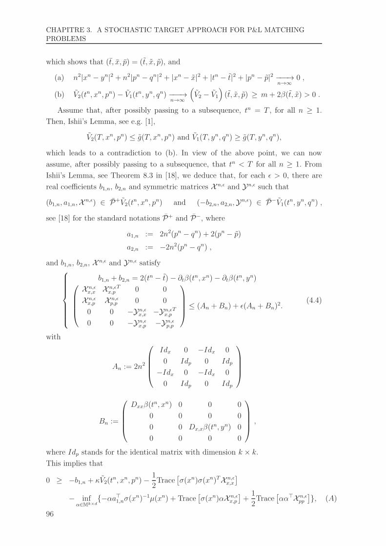
CHAPITRE 3. A STOCHASTIC TARGET APPROACH FOR P&L MATCHING
PROBLEMS
which shows that (t, x, p) = (t, x, p), and
(a) n2|xn − yn|2 + n2|pn − qn|2 + |xn − x|2 + |tn − t|2 + |pn − p|2 −−−→n→∞
0 ,
(b) V2(tn, xn, pn)− V1(t
n, yn, qn) −−−→n→∞
(V2 − V1
)(t, x, p) ≥ m+ 2β(t, x) > 0 .
Assume that, after possibly passing to a subsequence, tn = T , for all n ≥ 1.
Then, Ishii’s Lemma, see e.g. [1],
V2(T, xn, pn) ≤ g(T, xn, pn) and V1(T, y
n, qn) ≥ g(T, yn, qn),
which leads to a contradiction to (b). In view of the above point, we can now
assume, after possibly passing to a subsequence, that tn < T for all n ≥ 1. From
Ishii’s Lemma, see Theorem 8.3 in [18], we deduce that, for each ǫ > 0, there are
real coefficients b1,n, b2,n and symmetric matrices X n,ǫ and Yn,ǫ such that
(b1,n, a1,n,X n,ǫ) ∈ P+V2(tn, xn, pn) and (−b2,n, a2,n,Yn,ǫ) ∈ P−V1(t
n, yn, qn) ,
see [18] for the standard notations P+ and P−, where
a1,n := 2n2(pn − qn) + 2(pn − p)
a2,n := −2n2(pn − qn) ,
and b1,n, b2,n, X n,ǫ and Yn,ǫ satisfy
b1,n + b2,n = 2(tn − t)− ∂tβ(tn, xn)− ∂tβ(t
n, yn)
X n,ǫx,x X n,ǫ
x,pT 0 0
X n,ǫx,p X n,ǫ
p,p 0 0
0 0 −Yn,ǫx,x −Yn,ǫ
x,pT
0 0 −Yn,ǫx,p −Yn,ǫ
p,p
≤ (An +Bn) + ǫ(An +Bn)
2.(4.4)
with
An := 2n2
Idx 0 −Idx 0
0 Idp 0 Idp
−Idx 0 −Idx 0
0 Idp 0 Idp
Bn :=
Dxxβ(tn, xn) 0 0 0
0 0 0 0
0 0 Dx,xβ(tn, yn) 0
0 0 0 0
,
where Idp stands for the identical matrix with dimension k × k.
This implies that
0 ≥ −b1,n + κV2(tn, xn, pn)− 1
2Trace
[σ(xn)σ(xn)TX n,ǫ
x,x
]
− infα∈Mk×d
−αa⊤1,nσ(xn)−1µ(xn) + Trace[σ(xn)αX n,ǫ
x,p
]+
1
2Trace
[αα⊤X n,ǫ
pp
], (A)
96

4. ON THE UNBOUNDED CONTROL
We also obtain that
0 ≤ b2,n + κV1(tn, yn, qn)− 1
2Trace
[σ(yn)σ(yn)TYn,ǫ
x,x
]
−n2 infα∈Mk×d
2α(pn − qn)⊤σ(xn)−1µ(xn) + (1 + ǫ)Trace[αα⊤
]. (B)
We choose
αni,j := −(pnj − qnj )(σ−1µ)i,j(y
n)/(1 + ǫ)
so that the inferior in (B) achieves the minimum at αn and
−αn(pn − qn)⊤(σ−1µ)(yn) = (1 + ǫ)Trace[αn(αn)T
].
This, together with (A), implies that
0 ≥ −(b2,n + b1,n) + κ(V2(tn, xn, pn)− V1(t
n, yn, qn))
+1
2Trace
[σ(yn)σ(yn)TYn,ǫ
x,x
]− 1
2Trace
[σ(xn)σ(xn)⊤X n,ǫ
x,x
]
−2n2αn(pn − qn)⊤[(σ−1µ)(xn) + (σ−1µ)(yn)]
−αn(pn − p)⊤(σ−1µ)(xn).
Since σ−1µ is bounded in Rd, we take ǫ→ 0 and deduce that
0 ≥ −2(tn − t) + κ[V2(tn, xn, pn)− V1(t
n, yn, qn)− β(tn, xn)− β(tn, yn)]
−∂tβ(tn, xn) + κβ(tn, xn)− 1
2Trace
[σ(xn)σ(xn)⊤Dx,xβ(t
n, xn)]
−∂tβ(tn, yn) + κβ(tn, yn)− 1
2Trace
[σ(yn)σ(yn)⊤Dx,xβ(t
n, yn)]
+n2|σ(yn)− σ(xn)|2 − C(n2|pn − qn|2 + |pn − p|2)≥ κm+ λ(n),
where limn→∞
λ(n) = 0. This leads a contradiction. 2
97

CHAPITRE 3. A STOCHASTIC TARGET APPROACH FOR P&L MATCHING
PROBLEMS
98

Chapitre 4
The approximating problems and
numerical schemas
We shall see that both the associated Hamilton-Jacobi-Bellman operator and
the boundary conditions in Theorem 2.1 and Corollary 2.1 of previous chapter are
discontinuous, which leaves little hope to be able to establish a comparison result,
and therefore build a convergent numerical scheme directly based on this PDE cha-
racterization. We therefore introduce a sequence of approximating problems that are
more regular and for which we can prove comparison. We show that they converge
to the value function at any continuity point in the p-variable, or, more precisely,
to its right and left limits in the p-variable, depending on the chosen approximating
sequence. In particular, we will show that it allows to approximate point-wise the
relaxed problems :
v(t, x, p) (0.1)
:= inf
y : ∀ε > 0 ∃νε s.t. Y νε
t,x,y(T ) ≥ ℓ,
P[Y νε
t,x,y(T )− g(Xt,x(T )) ≥ −γi]≥ pi − ε ∀ i
and
v(t, x, p) (0.2)
:= infy : ∃ ν s.t. Y νt,x,y(T ) ≥ ℓ , P
[Y νt,x,y(T )− g(Xt,x(T )) ≥ −γi
]> pi ∀ i ≤ κ.
The first value function v is indeed shown to be the left-limit in p of v, while v is the
right-limit in p of v. In cases where v is continuous, then v = v = v and our schemes
converge to the original value function. However the continuity of v in its p-variable
seems are a-priori difficult to prove by lack of convexity and strict monotonicity of
the indicator function, and may fail in general. Still, one of the two approximations
can be chosen to solve practical problems.
99

CHAPITRE 4. THE APPROXIMATING PROBLEMS AND NUMERICAL SCHEMAS
Figure 4.1 – Function ∆iλ(x, ·)
1 The approximating problems
1.1 Definition and convergence properties
Set Λ := (0, (L−1 ∧ 1)/2)κ. Our approximating sequence (vλ)λ∈Λ is a sequence of
value functions associated to regularized stochastic target problems with controlled
loss. Namely, for λ ∈ Λ, we set
vλ(t, x, p)
:= infy ≥ ℓ : ∃ν ∈ U t s.t Y νt,x,y(T ) ≥ ℓ, E[∆i
λ(Xt,x(T ), Yνt,x,y(T ))] ≥ pi for i ∈ K,
where
∆iλ(x, y) =
0 if y < ℓλi(y−ℓ)
gi(x)−2λi−ℓ if ℓ ≤ y < gi(x)− 2λi
λi + (1−2λi)(y−gi(x)+2λi)λi
if gi(x)− 2λi ≤ y < gi(x)− λi
(1− λi) + λi(y−gi(x)+λi)gi(x)−gi(x)+λi if gi(x)− λi ≤ y < gi(x)
1 if y ≥ gi(x)
(1.1)
is well-defined for λ ∈ Λ = (0, (L−1 ∧ 1)/2)κ as in Figure 4.1, recall (2.7), (2.8) and
(2.11) of previous chapter.
100

1. THE APPROXIMATING PROBLEMS
The convergence (vλ)λ∈Λ as λ ↓ 0 is an immediate consequence of the linearity
of Y ν with respect to its initial condition.
Proposition 1.1 For all λ ∈ Λ and (t, x, p) ∈ [0, T ]× (0,∞)d × [0, 1]κ,
vλ(t, x, p⊕ λ) + 2maxi≤κ
λi ≥ v(t, x, p) ≥ vλ(t, x, p⊖ λ)−maxi≤κ
λi , (1.2)
where
p⊕ λ := (((pi + λi) ∧ 1) ∨ 0)i≤κ and p⊖ λ := (((pi − λi) ∧ 1) ∨ 0)i≤κ .
Proof. This follows easily from the linearity of Y ν with respect to its initial condition
and the fact that
1y−gi(x)+2λi≥0 + λi ≥ ∆iλ(x, y) ≥ 1y−gi(x)+λi≥0 − λi, for (y, x) ∈ R× (0,∞)d.
2
As an immediate consequence, we deduce that the sequences (vλ(·, ·⊕λ))λ∈Λ and
(vλ(·, · ⊖ λ))λ∈Λ allows to approximate v at any continuity points in its p-variable.
More precisely, the following holds.
Corollary 1.1 For all (t, x, p) ∈ [0, T ]× (0,∞)d × [0, 1]κ,
v(t, x, p−) = lim infλ↓0
vλ(t, x, p⊖ λ) and v(t, x, p+) = lim supλ↓0
vλ(t, x, p⊕ λ), (1.3)
where
v(·, p−) := limε↓0
v(·, p⊖ ε1κ) and v(·, p+) := limε↓0
v(·, p⊕ ε1κ)
with 1κ = (1, . . . , 1) ∈ Rκ.
Proving the continuity in its p-variable of the initial value function v by proba-
bilistic arguments, and therefore the point-wise convergence of our approximation
seems very difficult, and is beyond the scope of this paper. A standard approach
could be to derive the continuity of v by using its PDE characterization and by ap-
plying a suitable comparison theorem which would imply that v∗ = v∗. As explained
at the end of Subsection 2.3 of Chapter 3, this also does not seem to be feasible.
Note however that the right- and left-limits of v in its p-variable have interpre-
tations (0.1) and (0.2) in terms of natural relaxed version of the original problem
(2.9) in Chapter 3.
Proposition 1.2 For all (t, x, p) ∈ [0, T ]× (0,∞)d × (0, 1)κ,
v(t, x, p+) = v(t, x, p) ≥ v(t, x, p) = v(t, x, p−) .
Proof. It is obvious that v ≥ v ≥ v. Moreover, any y > v(t, x, p+ε1κ) for some ε > 0,
satisfies y ≥ v(t, x, p). Hence, for ε > 0 small enough, v(t, x, p+ ε1κ) ≥ v(t, x, p), so
that v(t, x, p+) ≥ v(t, x, p). Similarly, y > v(t, x, p) implies y ≥ v(t, x, p − ε1κ), for
any ε > 0 small enough, and therefore v(t, x, p) ≥ v(t, x, p−). 2
101

CHAPITRE 4. THE APPROXIMATING PROBLEMS AND NUMERICAL SCHEMAS
1.2 PDE characterization of the approximating problems
The reason for introducing the sequence approximating problems (vλ)λ∈Λ is that
they are more regular :
1. ∆λ is Lipschitz continuous :
|∆iλ(x, y + h)−∆i
λ(x, y)| ≤ Cλ|h|, for (x, y, h) ∈ (0,∞)d × R× R. (1.4)
where
Cλ := maxi∈K
maxλi/(L−1 − 2λi) , 1/λi , 1 , (1.5)
recall (2.8) and (2.11) of previous chapter.
2. Its inverse with respect to its y-variable is Lipschitz continuous too. Hence,
the natural boundary condition at T is given by a continuous function
Gλ(x, p) := infy ≥ ℓ : mini∈K
(∆iλ(x, y)− pi) ≥ 0. (1.6)
Item 2. above will allow us to prove that the boundary condition as t→ T is indeed
given by the continuous function Gλ, compare with 1. of Remark 2.13 in Chapter 3.
Proposition 1.3 The function vλ satisfies
vλ∗(T, ·) = vλ∗ (T, ·) = Gλ on (0,∞)d × [0, 1]κ. (1.7)
Proof. See Section 3 below. 2
Item 1. above induces a gradient constraint on vλ with respect its p-variable,
showing that it is strictly increasing with respect to this variable, in a suitable
sense, which will allow us to prove a comparison result for the related PDE, compare
with Remark 2.11 and 3. of Remark 2.13 in pervious chapter. We could not obtain
this for the original problem by lack of continuity and local strict monotonicity of
the indicator function. More precisely, we shall prove in Subsection 3.3 below the
following.
Proposition 1.4 Set
:= 4L2(T ∨ 1) . (1.8)
Fix (I, J) ∈ Pκ \Pκκ and assume that ι ≥ 0 is such that vλ∗IJ(t, x, p) > vλ∗JcJ(t, x, p)+ ι.
Let ϕ be a smooth function such that (t, x, p) achieves a maximum of vλ∗IJ −ϕ. Then,∑
i/∈I∪J
Dpiϕ ≥ ι
Cλ(ι+ )=: λ(ι) , (1.9)
where Cλ is defined as in (1.5).
102
1. THE APPROXIMATING PROBLEMS
Note that the above can be translated in terms of the operator MλIJ defined as :
(y, z, qp) ∈ R× R× Rκ 7→ MλIJ(y, z, qp) := max
ι≥0miny − z − ι , λ(ι)−
∑
i/∈I∪J
qip .
Corollary 1.2 Fix (I, J) ∈ Pκ \ Pκκ . Then v
λ∗IJ is a viscosity subsolution on DIJ of
MλIJ(ϕ, v
λ∗JcJ , Dpϕ) = 0 .
In view of Theorem 2.1 in [12], this implies that vλ is a discontinuous viscosity
solution of the system (Sλ) defined as follows, where we use the convention
MλIJ = −∞ for I ∪ J = K . (1.10)
Definition 1.1 Let V be a locally bounded map defined on D.
(i) We say that V is a discontinuous viscosity supersolution of (Sλ) if, for each
(I, J) ∈ Pκ, VIJ∗ is a viscosity supersolution on DIJ of
Hλ∗IJ [ϕ, VJcJ∗] (1.11)
:= maxmin
ϕ− ℓ , −∂tϕ+ F ∗
IJ(·, Dϕ,D2ϕ), Mλ
IJ(ϕ, VJcJ∗, Dpϕ)= 0 .
(ii) We say that V is a discontinuous viscosity subsolution of (Sλ) if, for each (I, J) ∈Pκ, V ∗
IJ is a viscosity subsolution on DIJ of
HλIJ∗[ϕ, V
∗JcJ ] (1.12)
:= maxmin
ϕ− ℓ , −∂tϕ+ FIJ∗(·, Dϕ,D2ϕ)
, Mλ
IJ(ϕ, V∗JcJ , Dpϕ)
= 0 .
(iii) We say that V is a discontinuous viscosity solution of (Sλ) if it is both a dis-
continuous super- and subsolution of (Sλ).
Remark 1.1 The convention (1.10) means that a supersolution of (1.11) (resp. a
subsolution of (1.12)) for I ∪ J = K is indeed a supersolution of (2.20) (resp. a
subsolution of (2.21)) of Chapter 3.
Remark 1.2 Note that a viscosity supersolution of (2.20) on DIJ is also a viscosity
supersolution of (1.11) on DIJ . As already argued,
vλ is a discontinuous solution of (S) (1.13)
by Theorem 2.1 in [12], so that Corollary 1.2 implies that it is a discontinuous
solution of (Sλ). From the supersolution point of view, the latter characterization is
weaker. Still we shall use it because, first, it is sufficient and, second, we shall appeal
to it when discussing the convergence of a finite difference approximation scheme
below.
103

CHAPITRE 4. THE APPROXIMATING PROBLEMS AND NUMERICAL SCHEMAS
Combining the above results, we obtain :
Theorem 1.1 The function vλ is a discontinuous viscosity solution of (Sλ). Moreo-
ver, it satisfies
vλ∗(T, ·) = vλ∗ (T, ·) = Gλ on (0,∞)d × [0, 1]κ. (1.14)
The fact that the above Theorem allows to characterize uniquely vλ is a conse-
quence of the following comparison result, in the viscosity sense.
Theorem 1.2 (i) Let V be a bounded function on [0, T ) × (0,∞)d × [0, 1]κ which
is non-decreasing with respect to its last parameter. Assume that V is a disconti-
nuous viscosity supersolution of (Sλ) such that V∗(T, ·) ≥ Gλ and VIJ∗ ≥ VI′J ′∗ on
∂DIJ ∩DI′J ′ for all (I, J), (I ′, J ′) ∈ Pκ such that (I ′, J ′) ) (I, J). Then, V ≥ vλ on
D.
(ii) Let V be a bounded function on [0, T )× (0,∞)d× [0, 1]κ which is non-decreasing
with respect to its last parameter. Assume that V is a discontinuous viscosity sub-
solution of (Sλ) such that V ∗(T, ·) ≤ Gλ and V ∗IJ ≤ V ∗
I′J ′ on ∂DIJ ∩ DI′J ′ for all
(I, J), (I ′, J ′) ∈ Pκ such that (I ′, J ′) ) (I, J). Then, V ≤ vλ on D.
Proof. See Subsection 3.5 below. 2
Combining the above results leads to the following characterization.
Theorem 1.3 The function vλ is continuous and is the unique bounded disconti-
nuous viscosity solution of the system (Sλ) in the class of bounded discontinuous
solutions V which are non-decreasing in their last variable and satisfy V∗(T, ·) =
V ∗(T, ·) = Gλ, V ∗IJ ≤ V ∗
I′J ′ and VIJ∗ ≥ VI′J ′∗ on ∂DIJ ∩DI′J ′ for all (I, J), (I ′, J ′) ∈Pκ such that (I ′, J ′) ) (I, J).
2 Finite differences approximation
In this section, we construct an explicit finite difference scheme and prove its
convergence.
2.1 PDE reformulation
We first reformulate the PDEs associated to vλ in a more tractable way, which
will allow us to define naturally a monotone scheme. To this purpose, we introduce
104

2. FINITE DIFFERENCES APPROXIMATION
the support function δU associated to the closed convex (and bounded) set U as in
(2.24) of Chapter 3. Since 0 ∈ intU , δU characterizes U in the following sense
u ∈ intU iff min|ζ|=1
(δU(ζ)− ζ⊤u) > 0 and u ∈ U iff min|ζ|=1
(δU(ζ)− ζ⊤u) ≥ 0 ,
see e.g. Rockafellar [39].
Moreover (u, a) ∈ N ǫIJ(x, q) with q
⊤ = (q⊤x , q⊤p ), if and only if there exists ξǫ ∈ Rd
such that |ξǫ| ≤ ǫ for which
u⊤ = u(x, a, q)⊤ + ξǫσ(x)−1 ∈ U and a ∈ AIJ ,
where
u(x, q, a)⊤ := q⊤x diag[x] + q⊤p aσ(x)−1.
It follows that
−r + F ∗IJ(x, q, Q) ≥ 0 iff K∗
IJ(x, r, q, Q) ≥ 0
and
−r + FIJ∗(x, q, Q) ≤ 0 iff KIJ∗(x, r, q, Q) ≤ 0
where K∗IJ and KIJ∗ are the upper- and lower-semicontinuous envelopes of
KIJ(x, r, q, Q) := supa∈AIJ
min−r + Lu(x,q,a),a(x, q, Q) , Ra(x, q)
with
Ra(x, q) := inf|ζ|=1
Ra,ζ(x, q) and Ra,ζ(x, q) := δU(ζ)− ζ⊤u(x, q, a) .
Remark 2.1 For later use, note that, for q⊤ = (q⊤x , q⊤p ),
Lu(x,q,a),a(x, q, Q) = q⊤p aσ(x)−1µ(x)− 1
2Ξa(x,Q) =: La(x, qp,Ξ
a(x,Q)).
where
Ξa(x,Q) := Trace[σX,Pσ
⊤X,P (x, a)Q
],
does not depend on qx.
It follows that V is a viscosity supersolution of (1.11) if and only if it is a viscosity
supersolution of
Hλ∗IJ [ϕ, VJcJ∗] (2.1)
:= maxmin
ϕ− ℓ , K∗
IJ(·, ∂tϕ,Dϕ,D2ϕ), Mλ
IJ(ϕ, VJcJ∗, Dpϕ)= 0 ,
and that V is a viscosity subsolution of (1.12) if and only if it is a viscosity subso-
lution of
HλIJ∗[ϕ, V
∗JcJ ] (2.2)
:= maxmin
ϕ− ℓ , KIJ∗(·, ∂tϕ,Dϕ,D2ϕ)
, Mλ
IJ(ϕ, V∗JcJ , Dpϕ)
= 0.
105

CHAPITRE 4. THE APPROXIMATING PROBLEMS AND NUMERICAL SCHEMAS
2.2 Scheme construction
We now define a monotone finite difference scheme for the formulation obtained
in the previous section. In the following, we write h to denote an element of the form
h = (h0, h1, h2) ∈ (0, 1)3.
a. The discretization in the time variable.
Given n0 ∈ N, we first introduce a discretization time-step h0 := T/n0 together
with a grid
Th := (T − (n0 − i)h0), i = 0, . . . , n0.
The time derivative is approximated as usual by
∂ht [ϕ](t, x, p) := h−10 (ϕ(t+ h0, x, p)− ϕ(t, x, p)) .
b. Discretization in the space variable.
The grids in the space variables are defined as
XhcX
:= e−cX+(n−i)h1 , i = 0, . . . , nXd and Ph := 1− (n− i)h1, i = 0, . . . , nPκ ,
for some cX , n ∈ N and where h1 := 1/n, (nX , nP ) := n(2cX , 1).
Note that the space discretization in the x variable amounts to performing a
logarithmic change of variable. Taking this into account, the first order derivatives
with respect to x and p are then approximated as follows, with eii≤d (resp. ℓjj≤κ)denoting the canonical basis of Rd (resp. Rκ) :
∂L,hp,j [ϕ, a](t, x, p) := h−11
ϕ(t+ h0, x, p⊕ h1ℓj)− ϕ(t, x, p) if µ⊤(aσ−1(x))⊤ℓj ≤ 0
ϕ(t, x, p)− ϕ(t+ h0, x, p⊖ h1ℓj) if µ⊤(aσ−1(x))⊤ℓj > 0
∂R,hx,i [ϕ, ζ ](t, x, p) := h−11 diag [x]−1
ϕ(t+ h0, x⊕h1ei, p)− ϕ(t, x, p) if e⊤i ζ ≥ 0
ϕ(t, x, p)− ϕ(t+ h0, x⊖h1ei, p) if e⊤i ζ < 0
∂R,hp,j [ϕ, a, ζ ](t, x, p) := h−11
ϕ(t + h0, x, p⊕ h1ℓj)− ϕ(t, x, p) if ℓ⊤j aσ
−1(x)ζ ≥ 0
ϕ(t, x, p)− ϕ(t+ h0, x, p⊖ h1ℓj) if ℓ⊤j aσ
−1(x)ζ < 0
∂M,hp,j [ϕ](t, x, p) := h−1
1 (ϕ(t+ h0, x, p⊕ h1ℓj)− ϕ(t, x, p)),
where the operators ⊕ and ⊖ are given in Proposition 1.1 and
x⊕y := ((xieyi
) ∨ e−cX) ∧ ecX )i≤d
and
x⊖y := ((xie−yi
) ∨ e−cX) ∧ ecX )i≤d,106

2. FINITE DIFFERENCES APPROXIMATION
for (x, y) ∈ (0,∞)d × Rd.
We denote by ∂L,hp , ∂K,hx , ∂K,hp and ∂M,hp the corresponding vectors.
As for the second order term, we use the Camilli and Falcone approximation [16],
in order to ensure that the scheme is monotone. Namely, we first introduce an ap-
proximation parameterized by h2 > 0 of Trace[σ(X,P )σ
⊤(X,P )(x, a)D
2ϕ(t + h0, x, p)]
as follows
∆h[ϕ, a](t, x, p) := h−12
d∑
i=1
ϕ(t+ h0, x⊕√h2σ
·i(x), p⊕√h2a
·i)
+h−12
d∑
i=1
ϕ(t+ h0, x⊖√h2σ
·i(x), p⊖√h2a
·i)
−2h−12
d∑
i=1
ϕ(t+ h0, x, p)
−h−11
d∑
i=1
|σ·i(x)|2(ϕ(t0, x, p)− ϕ(t+ h0, x⊖h1ei, p)
)(2.3)
where σ·i and a·i denote the i-th column of σX and a.
Note that the above approximation of the second order term requires the compu-
tation of the approximated value function at points outside of the grid. It therefore
requires an interpolation procedure. In this paper, we use a local linear interpola-
tion based on the Coxeter-Freudenthal-Kuhn triangulation, see e.g. [36]. It consists
in first constructing the set of simplices Sjj associated to the regular triangulation
of ln[e−cX , ecX ]d × [0, 1]κ with the set of vertices lnXhcX
× Ph. Here the ln operator
means that we take the ln component-wise, recall that we use a logarithmic scale.
In such a way, we can then provide an approximating function belonging to the
set Sh of the functions which are continuous in [e−cX , ecX ]d × [0, 1]κ and piecewise
affine inside each simplex Sj (in ln scale for the x-variable). More precisely, each
point (y, p) ∈ [−cX , cX ]d× [0, 1]κ can be expressed as a weighted combination of the
corners of the simplex Sj it lies in. We can thus write
(y, p) =∑
ζ∈lnXhcX
×Ph
ω(y, p | ζ)ζ,
where ω is a non negative weighting function such that
∑
ζ∈lnXhcX
×Ph
ω(y, p |ζ) = 1.
Given a map ϕ defined on Th × XhcX
× Ph , we then approximate it at (t, x, p) ∈Th × [e−cX , ecX ]d × [0, 1]κ by
ϕ(t, x, p) :=∑
(ζX ,ζP )∈lnXhcX
×Ph
ω(lnx, p | ζ)ϕ(t, eζX , ζP )
107

CHAPITRE 4. THE APPROXIMATING PROBLEMS AND NUMERICAL SCHEMAS
in which the exponential is taken component by component.
This leads to the approximation of ∆h[ϕ, a](t, x, p) by
∆h[ϕ, a](t, x, p)
:= h−12
d∑
i=1
∑
(ζX ,ζP )∈lnXhcX
×Ph
ω(xih+, pih+[a] |(ζX, ζP ))ϕ(t + h0, e
ζX , ζP )
+h−12
d∑
i=1
∑
(ζX ,ζP )∈lnXhcX
×Ph
ω(xih−, pih−[a] |(ζX , ζP ))ϕ(t+ h0, e
ζX , ζP )
−2dh−12 ϕ(t+ h0, x, p)
−h−11
d∑
i=1
|σ·i(x)|2(ϕ(t+ h0, x, p)− ϕ(t+ h0, x⊖h1ei, p)
)
where
xih+ := x⊕√h2σ
·i(x) , pih+[a] := p⊕√h2a
·i,
and
xih− := x⊖√h2σ
·i(x) , pih−[a] := p⊖√h2a
·i.
c. The approximated operator.
Given a > 0, we then approximate HλIJ by Hh,cX ,a
IJ defined as
Hh,cX ,aIJ [ϕ, ψ] := max
min
ϕ− ℓ , sup
a∈AaIJ
Kahϕ
, M IJ
h [ϕ, ψ]
with
AaIJ := a ∈ AIJ : |a| ≤ a, M IJh [ϕ, ψ] :=M IJ(ϕ, ψ, ∂M,h
p [ϕ])
and
Kahϕ := min
−∂L,ht ϕ+ La(·, ∂L,hp ϕ,∆L,h[ϕ, a]) , min
|ζ|=1Ra,ζ(·, ∂R,hx [ϕ, ζ ], ∂R,hp [ϕ, a, ζ ])
.
The resolution is done as follows :
(i). For (I, J) ∈ Pκκ , we define wa,cX ,hIJ ∈ Sh as the solution of
wa,cX ,hIJ (T, ·) = Gλ(·, πIJ) on XhcX
×Ph
maxwa,cX ,hIJ − L , Hh,cX ,aIJ [wa,cX ,hIJ , 0] = 0 on Th
− ×XhcX− ×Ph
wa,cX ,hIJ = gJ on Th− × (Xh
cX\Xh
cX−)×Ph
.
where we use the notations
Th− := (T − (n0 − i)h0), i = 0, . . . , n0 − 1
108

2. FINITE DIFFERENCES APPROXIMATION
XhcX− := e−cX+(n−i)h1 , i = 1, . . . , nX − 1d,
and
Dh− := Th
− ×XhcX− ×Ph.
(ii).We then proceed by backward induction on |I|+|J |. Once wa,cX ,hI′J ′ ∈ Sh construc-ted for (I ′, J ′) ∈ P l
κ for all l ≥ k, for some 1 ≤ k ≤ κ, we define wa,cX ,hIJ for
(I, J) ∈ Pk−1κ as the solution of
wa,cX ,hIJ (T, ·) = Gλ(·, πIJ) on XhcX
×Ph
(wa,cX ,hIJ − wa,cX ,hJcJ ) ∧maxwa,cX ,hIJ − L , Hh,cX ,aIJ [wa,cX ,hIJ , wa,cX ,hJcJ ] = 0 on Dh
− ∩DIJ
wa,cX ,hIJ = gJ on (Th− × (Xh
cX\Xh
cX−)×Ph) ∩DIJ
wa,cX ,hIJ = wa,cX ,hI′J ′ on Dh− ∩ ∂DIJ ∩DI′J ′ for (I ′, J ′) ) (I, J)
One easily checks that
|∆h[ϕ, a](t, x, p)−∆h[ϕ, a](t, x, p)| ≤ O(h1/h2), (2.4)
which implies that the numerical scheme is monotone and consistent whenever
h0 = o(h1) and h1 = o(h2). (2.5)
2.3 Convergence of the approximating scheme
The convergence of the scheme is obtained as h = (h0, h1, h2) → 0 and cX → ∞,
with the convention (2.5), and then a → ∞. We therefore define the relaxed semi-
limits, for (t, x, p) ∈ DIJ , (I, J) ∈ Pκ,
wa∗IJ(t, x, p) := lim sup(t′, x′, p′) → (t, x, p)
h → 0, cX → ∞
wa,cX ,hIJ (t′, x′, p′) ,
waIJ∗(t, x, p) := lim inf(t′, x′, p′) → (t, x, p)
h → 0, cX → ∞
wa,cX ,hIJ (t′, x′, p′)
and
w∗IJ(t, x, p) := lim sup
(t′, x′, p′) → (t, x, p)
a → ∞
wa∗IJ(t′, x′, p′) ,
wIJ∗(t, x, p) := lim inf(t′, x′, p′) → (t, x, p)
a → ∞
waIJ∗(t′, x′, p′) ,
in which the limits are taken along sequences of points (t′, x′, p′) ∈ DIJ and h
satisfying (2.5). Note that wa,cX ,hIJ takes values in [ℓ, L], so that the above are well-
defined and bounded. Moreover, it is convergent :
Theorem 2.1 For all (I, J) ∈ Pκ, w∗IJ = wIJ∗ = vλIJ on DIJ .
109

CHAPITRE 4. THE APPROXIMATING PROBLEMS AND NUMERICAL SCHEMAS
Proof. See Subsection 4.2 below. 2
We conclude this section with some numerical illustration in the Black and
Scholes model, where the stock price X is defined as
Xt,x(s) = x+
∫ s
t
Xt,x(r)dWr for s ∈ [t, 1],
the payoff g(X) = (K − X)+ with the strike price K = 3, the thresholds γ =
γ1, γ2 = 0, 0.5.
Example 2.1 We study the case U = [−1, 1].
00.1
0.20.3
0.40.5
0.60.7
0.80.9
1
00.1
0.20.3
0.40.5
0.60.7
0.80.9
1
−1
−0.5
0
0.5
1
1.5
P2P1
Figure 4.2 – vλ with U = [−1, 1]
Then, the “face-lifted” version of g is defined by
g(x) =
3− x if x ∈ (0, 1]
2− ln(x) if x ∈ [1, e2]
0 if x ≥ e2.
Taking λ = 1/32 and ℓ = −1, the Figure 4.2 plots an estimated value of vλ(0, x, p1, p2)
when we fix x = e.
110

3. PROOF OF THE PDE CHARACTERIZATIONS
Example 2.2 When U = [−5, 5], the “face-lifted” version of g is equal to g on R+.
The Figure 4.3 plots an estimated value of vλ(0, x, p1, p2) when we take λ = 1/32,
ℓ = −1 and x = 1. In the Figure 4.4, we describe its graph when p2 = 0 in the same
setting.
00.1
0.20.3
0.40.5
0.60.7
0.80.9
1
00.1
0.20.3
0.40.5
0.60.7
0.80.9
1
−1
−0.5
0
0.5
1
1.5
2
P2P1
Figure 4.3 – vλ with U = [−5, 5]
3 Proof of the PDE characterizations
In this section, we collect the proofs of Proposition 1.3, Proposition 1.4, Theorem
1.2, Theorem 1.3 and Theorem 2.1. The boundary conditions in the space variable
p follows the same argument as in Section 3 in the previous chapter. It remains to
prove the boundary conditions in time and the gradient estimates in the viscosity
sense We first recall the geometric dynamic programming principle of [46], see also
[47] and [49], to which we will appeal to prove the boundary conditions. We next
report the proof of the supersolution properties in subsection 3.2, and that of the
subsolution properties in subsection 3.1. The gradient estimates in the viscosity
sense and the corresponding comparison result are proved in next subsection.
111

CHAPITRE 4. THE APPROXIMATING PROBLEMS AND NUMERICAL SCHEMAS
00.1
0.20.3
0.40.5
0.60.7
0.80.9
1
−1−0.8
−0.6−0.4
−0.20
0.20.4
0.60.8
1
−1
−0.5
0
0.5
1
1.5
2
2.5
3
P1ln X
Figure 4.4 – U=[-5,5] and p2 = 0
Corollary 3.1 Fix (t, x, p) ∈ DIJ .
(GDP1’) If y ≥ ℓ and (ν, α) ∈ Ut ×AIJt,πIJ(p)
are such that
∆λ(Xt,x, (T ), Yνt,x,y(T )) ≥ P α
t,p(T )
then
Y νt,x,y(θ) ≥ vλIJ(θ,Xt,x(θ), P
αt,p(θ)) , for all θ ∈ T t
[t,T ] .
(GDP2’) For y < vλIJ(t, x, p), θ ∈ T t[t,T ] and (ν, α) ∈ Ut ×AIJ
t,πIJ(p),
P[Y νt,x,y(θ) > vλIJ(θ,Xt,x(θ), P
αt,p(θ))
]< 1.
3.1 Boundary condition for the upper-semicontinuous enve-
loppe
We start with the boundary condition as t→ T .
Proposition 3.1 For all (I, J), (I ′, J ′) ∈ Pκ such that (I ′, J ′) ⊃ (I, J), we have
vλ∗IJ(T, ·) ≤ Gλ on (0,∞)d × BI′J ′.
112

3. PROOF OF THE PDE CHARACTERIZATIONS
Proof.
Step 1. We first show that the required result is true if I ∪ J = K. Note that, in
this case, I ′ = I and J ′ = J . Then,
vλIJ = w := infy ≥ ℓ : ∃ ν ∈ U s.t. Y ν·,y(T ) ≥ gJ(X·(T )) .
Hence, it suffices to show that
w∗(T, ·) ≤ gJ , (3.1)
where w∗(T, x) := limε→0 supw(t′, x′) : (t′, x′) ∈ (T − ε, T ] × Bε(x′). We only
sketch the proof of (3.1) as it follows from the same arguments as in [9], up to obvious
modifications. In the following, we let (tn, xn)n be a sequence in [0, T )×(0,∞)d such
that (tn, xn) → (T, x) and w(tn, xn) → w∗(T, x).
It follows from the dual formulation of [22] that, for each n ≥ 1, we can find a
predictable process ϑn with values in Rd such that
Hϑn
n := E(−∫ ·
tn
σ−1X (µX − ϑns )(Xn(s))dWs
)
T
∈ L1(P) ,
where Xn := Xtn,xn, and
w(tn, xn) ≤ E
[Hϑn
n (T )
(gJ(Xn(T ))−
∫ T
tn
δU (ϑns )ds
)]+ n−1 .
Since δU is homogeneous of degree 1 and convex, this implies that
w(tn, xn) ≤ E
[Hϑn
n (T )
(gJ(Xn(T ))− δU(
∫ T
tn
ϑns )ds
)]+ n−1
so that, by definition of gJ in (2.23),
w(tn, xn) ≤ E[Hϑn
n (T )gJ(Zϑn
n (T ))]+ n−1 ,
where Zn := Xne−∫ ·
tnϑns ds. It remains to prove that
lim supn→∞
E[Hϑn
n (T )gJ(Zϑn
n (T ))]≤ gJ(x) .
To show this, it suffices to follow line by line the arguments contained after the
equation (6.7) in the proof of Proposition 6.7 in [9].
Step 2. We now consider the case I ∪ J 6= K. We assume that
y0 := vλ∗IJ(T, x, p) > Gλ(x, p) (3.2)
and work towards a contradiction. It follows from Step 1 that gJ ′(x) ≥ vλ∗J ′cJ ′(T, x). In
view of (3.2) and (1.6), this leads to vλ∗IJ(T, x, p) > vλ∗J ′cJ ′(T, x). Hence, there exists a
113

CHAPITRE 4. THE APPROXIMATING PROBLEMS AND NUMERICAL SCHEMAS
sequence (tn, xn, pn)n ⊂ DIJ which converges to (T, x, p) such that vλIJ(tn, xn, pn) →vλ∗IJ(T, x, p) and
vλ∗J ′cJ ′(tn, xn, pn) < vλ∗J ′cJ ′(T, x, p) + ǫ < yn for all n ≥ 1, for some ǫ > 0,
where yn := vλIJ(tn, xn, pn)− n−1. We can then find νn ∈ U such that
Yn(T ) ≥ gJ ′(Xn(T )) ≥ ℓ ,
where (Xn, Yn) := (Xtn,xn, Yνntn,xn,yn). Moreover, since ∆l
λ is strictly increasing on
(x′, y′) : ∆lλ(x
′, y′) ∈ (0, 1) and y0 > Gλ(x, p), we have ∆lλ(x, y0) > pl for
l /∈ I ′ ∪ J ′. Since (Xn(T ), Yn(T )) → (x, y0) in law, up to a subsequence, be-
cause U is bounded and by the Lipschitz continuity of (µX , σX), we deduce that
E[∆lλ(Xn(T ), Yn(T ))] ≥ pln for l /∈ I ′ ∪ J ′, and n large enough. Finally, Yn(T ) ≥ ℓ
so that E[∆lλ(Xn(T ), Yn(T ))] ≥ 0 for l ∈ I ′. This contradicts the fact that yn <
vλIJ(tn, xn, pn). 2
We now turn to the boundary condition in the p-variable, i.e. as p→ ∂BIJ .
Proposition 3.2 For all (I, J), (I ′, J ′) ∈ Pκ such that (I ′, J ′) ⊃ (I, J), we have
vλ∗IJ ≤ vλ∗I′J ′ on DI′J ′.
Proof. The proof follows the same argument as in Proposition 3.1 of the previous
chapter.
3.2 Boundary condition for the lower-semicontinuous enve-
lope
We start with the boundary condition as t→ T .
Proposition 3.3 For all (I, J), (I ′, J ′) ∈ Pκ such that (I ′, J ′) ⊃ (I, J), we have
vλIJ∗(T, ·) ≥ Gλ on (0,∞)d × BI′J ′.
Proof. Fix (x, p) ∈ (0,∞)d × BI′J ′ . Since vλIJ∗ ≥ ℓ, the required result is trivial
when p = 0. We thus consider the case where p 6= 0, and fix l ∈ K such that that
pl > 0. Let (tn, xn, pn)n ⊂ DIJ be a sequence that converges to (T, x, p) and such
that vλIJ(tn, xn, pn) → vλIJ∗(T, x, p). We define yn := vλIJ(tn, xn, pn) + n−1 so that, for
each n, there exists (νn, αn) ∈ U × Atn,pn satisfying yn + Yn(T ) ≥ ℓ and
E[∆lλ(Xn(T ), Yn(T ))] ≥ pln ,
where (Xn, Yn) := (Xtn,xn, Yνntn,xn,yn). Using the fact that U is bounded and that
(µX , σX) is Lipschitz continuous, one easily checks that, after possibly passing to a
114

3. PROOF OF THE PDE CHARACTERIZATIONS
subsequence, (Xn(T ), Yn(T )) converges to (x, vλIJ∗(T, x, p)) P−a.s. and in law. Since
∆λ is continuous, this implies that
∆lλ(x, v
λIJ∗(T, x, p)) ≥ pl > 0 .
By arbitrariness of l such that pl 6= 0, this leads to the required result. 2
In order to discuss the boundary condition in the p-variable, we follow [12]
and first provide a supersolution property for vλIJ on the boundary DIJ ∩ DI′J ′
for (I ′, J ′) ⊃ (I, J). A more precise statement will be deduced from the following
one and the comparison result of Proposition 3.6 below, see Subsection 3.5.
Proposition 3.4 For all (I, J), (I, J ′) ∈ Pκ such that J ′ ⊃ J , vλIJ∗ is a supersolu-
tion on DIJ of
minϕ− ℓ, −∂tϕ+ F ∗IJ ′ϕ ≥ 0 on DIJ ′. (3.3)
Proof. The proof follows the same argument as in Proposition 3.2 of the previous
chapter.
3.3 Gradient estimates
In this section, we prove Proposition 1.4. It is based on the following growth
estimate.
Proposition 3.5 Fix (I, J), (I ′, J ′) ∈ Pκ such that I ∪ J 6= K and J ⊂ J ′. Let
(t, x, p) ∈ DIJ be such that (vλIJ − vλI′J ′)(t, x, p) > ι ≥ 0. Let > 0 be defined as in
(1.8). Then,
vλIJ(t, x, p)− vλIJ (t, x, p⊖ Cλδ(ι+ )1IJ) ≥ δι for all 0 ≤ δ ≤ 1 , (3.4)
where 1IJ stands for (1i/∈I∪J)i≤κ.
Proof. Fix (t, x, p) ∈ DIJ , y > vλIJ(t, x, p) and ι ≥ 0 such that vλIJ(t, x, p) − ι >
vλI′J ′(t, x, p). Then, we can find ν ∈ U such that
Y νt,x,y(T ) ≥ ℓ and E[∆i
λ(Xt,x(T ), Yνt,x,y(T ))] ≥ pi for alli ≤ κ,
and ν ′ ∈ U such that
Y ν′
t,x,y−ι(T ) ≥ ℓ andY ν′
t,x,y−ι(T ) ≥ gj(Xt,x(T )) for allj ∈ J ′,
recall (1.1).
Set νδ := (1− δ)ν + δν ′ ∈ U , recall that U is convex, and yδ := (1− δ)y+ δ(y− ι) =
y − δι. Note that
Y νδt,x,yδ
(T ) = (1− δ)Y νt,x,y(T ) + δY ν′
t,x,y−ι(T ) ,
115

CHAPITRE 4. THE APPROXIMATING PROBLEMS AND NUMERICAL SCHEMAS
by (2.4). Combined with the above inequalities and the fact that pi = 1 for i ∈ J ⊂J ′, this readily implies that
Y νδt,x,yδ
(T ) ≥ ℓ and Y νδt,x,yδ
(T ) ≥ gi(Xt,x(T )) for i ∈ J . (3.5)
Since ∆iλ is Cλ-Lipschitz with respect to y, see (1.4), we also have
E[∆iλ(Xt,x(T ), Y
νδt,x,yδ
(T ))]
= E[∆iλ
(Xt,x(T ), Y
νt,x,y(T ) + δ(Y ν′
t,x,y−ι(T )− Y νt,x,y(T ))
)]
≥ E[∆iλ(Xt,x(T ), Y
νt,x,y(T ))]− CλδE
[|Y ν′
t,x,y−ι(T )− Y νt,x,y(T )|
]
≥ pi − CλδE[|Y ν′
t,x,y−ι(T )− Y νt,x,y(T )|
], for i /∈ J ,
where
E[|Y ν′
t,x,y−ι(T )− Y νt,x,y(T )|
]
≤ ι+ E
[∣∣∣∣∫ T
t
(νs − ν ′s)⊤µ(Xt,x(s))ds+
∫ T
t
(νs − ν ′s)⊤σ(Xt,x(s))dWs
∣∣∣∣].
Recalling (2.2) and (2.3), standard estimates imply that the right-hand side term is
bounded by as defined in (1.8). Hence
E[∆iλ(Xt,x(T ), Y
νδt,x,yδ
(T ))] ≥ pi − Cλδ (ι+ ) , for i /∈ J . (3.6)
We now combine (3.5) and (3.6) to deduce that
yδ ≥ vλIJ (t, x, p⊖ Cλδ (ι+ ) 1IJ) .
By arbitrariness of y > vλIJ(t, x, p), this implies the required result. 2
Proof of Proposition 1.4.
Fix (I, J) ∈ Pκ and (t, x, p) ∈ DIJ such that vλ∗IJ(t, x, p) > vλ∗JcJ(t, x, p) + ι for
some ι ≥ 0. Let ϕ be a smooth function and assume that (t, x, p) achieves the
maximum of vλ∗IJ − ϕ.
Since vλIJ is non-decreasing with respect to its p-variable, and by definition of
vλ∗JcJ , there exists (tn, xn, pn) → (t, x, p) such that vλIJ(tn, xn, pn) → vλ∗IJ(t, x, p) and
vλIJ(tn, xn, pn + Cλδ(ι+ )1IJ) > vλJcJ(tn, xn, pn + Cλδ(ι+ )1IJ) + ι for δ > 0 small
enough. By applying Proposition 3.5 at the point (tn, xn, pn + Cλδ(ι + )1IJ) for
(I ′, J ′) = (Jc, J), we deduce that
vλIJ(tn, xn, pn + Cλδ(ι+ )1IJ)− vλIJ (tn, xn, pn) ≥ δι ,
and therefore
ϕ(t, x, p+ Cλδ(ι+ )1IJ)− ϕ (t, x, p) ≥ δι .
Dividing by δ and sending δ to 0 leads to the required result for defined as in
(1.9) above. 2
116

3. PROOF OF THE PDE CHARACTERIZATIONS
3.4 Comparison results for the system of PDEs (Sλ)
We provide a comparison result for (Sλ). Additional technical improvements will
be considered in the next section to discuss the convergence of the numerical scheme
defined in Section 2.
Proposition 3.6 Let ψ1 ≥ ψ2 be two functions such that ψ1 and −ψ2 are lower-
semicontinuous. Fix (I, J) ∈ Pκ. Let V1 be a bounded lower-semicontinuous viscosity
supersolution of
Hλ∗IJ [ϕ, ψ1] = 0 on DIJ , (3.7)
and let V2 be a bounded upper-semicontinuous viscosity subsolution of
HλIJ∗[ϕ, ψ2] = 0 on DIJ . (3.8)
Assume that V1 ≥ V2 on ∂DIJ . Assume further that either V1 ≥ ψ2 on DIJ or that
(I, J) ∈ Pκκ . Then, V1 ≥ V2 on DIJ .
Proof.
Part 1 : (I, J) /∈ Pκκ . As usual, we first fix ρ > 0 and introduce the functions
V1(t, x, p) := eρtV1(t, x, p) and V2(t, x, p) := eρtV2(t, x, p). Arguing by contradiction,
we assume that
supDIJ
(V2 − V1) =: m > 0.
and work towards a contradiction.
1. For n, k ≥ 1 and ε > 0, we then define the function Ψkn,ε on [0, T ]×R2n × [0, 1]2κ
by
Ψkn,ε(t, x, y, p, q) := V2(t, x, p)− V1(t, y, q)−Θk
n,ε(t, x, y, p, q),
where
Θkn,ε(t, x, y, p, q) :=
n2
2|x− y|2 + k2
2|p− q|2 + fε(x),
with
fε(x) := ε
(|x|2 +
∑
i≤d
(xi)−1
).
It follows from the boundedness of V2 and V1 that Ψkn,ε achieves its maximum at
some (tkn,ε, xkn,ε, y
kn,ε, p
kn,ε, q
kn,ε) ∈ [0, T ]× (0,∞)2d × B2
IJ . Similarly, the map
(t, x, p, q) ∈ [0, T ]× (0,∞)d × B2IJ 7→ V2(t, x, p)− V1(t, x, q)−
k2
2|p− q|2 − fε(x)
117

CHAPITRE 4. THE APPROXIMATING PROBLEMS AND NUMERICAL SCHEMAS
achieves a maximum at some (tkε , xkε , p
kε , q
kε ) ∈ [0, T ]× (0,∞)d × B2
IJ . Moreover, the
inequality
Ψkn,ε(t
kn,ε, x
kn,ε, y
kn,ε, p
kn,ε, q
kn,ε) ≥ Ψk
n,ε(tkε , x
kε , x
kε , p
kε , q
kε )
implies that
V2(tkn,ε, x
kn,ε, p
kn,ε)− V1(t
kn,ε, y
kn,ε, q
kn,ε) ≥ V2(t
kε , x
kε , p
kε)− V1(t
kε , x
kε , q
kε )
−k2
2|pkε − qkε |2 − fε(x
kε) + fε(x
kn,ε)
+n2
2|xkn,ε − ykn,ε|2 +
k2
2|pkn,ε − qkn,ε|2.
Using the boundedness of V2 and V1 again together with the fact that BIJ is com-
pact, we deduce that the term on the second line is bounded in n so that, up to a
subsequence,
(tkn,ε, xkn,ε, y
kn,ε, p
kn,ε, q
kn,ε) → (tkε , x
kε , x
kε , p
kε , q
kε ) as n→ ∞,
for some (tkε , xkε , p
kε , q
kε ) ∈ [0, T ]× (0,∞)d × B2
IJ . By sending n→ ∞ in the previous
inequality, we also obtain
V2(tkε , x
kε , p
kε)− V1(t
kε , x
kε , q
kε )−
k2
2|pkε − qkε |2 − fε(x
kε)
≤ V2(tkε , x
kε , p
kε)− V1(t
kε , x
kε , q
kε )−
k2
2|pkε − qkε |2 − fε(x
kε)− lim inf
n→∞
n2
2|xkn,ε − ykn,ε|2.
It then follows from the maximum property at (tkε , xkε , p
kε , q
kε ) that the last term on
the right-hand side converges to 0 and that we can assume, without loss of generality,
that (tkε , xkε , p
kε , q
kε ) = (tkε , x
kε , p
kε , q
kε ), i.e.
(tkn,ε, xkn,ε, y
kn,ε, p
kn,ε, q
kn,ε) −−−→
n→∞(tkε , x
kε , x
kε , p
kε , q
kε ) and n
2|xkn,ε − ykn,ε|2 −−−→n→∞
0. (3.9)
It follows from similar arguments that we could choose (xkε)ε>0 such that, up to a
subsequence,
fε(xkε) −−→
ε→00 and (tkε , p
kε , q
kε ) −−→
ε→0(tk, pk, qk), (3.10)
and
limε→0
limn→∞
Ψkn,ε(t
kn,ε, x
kn,ε, y
kn,ε, p
kn,ε, q
kn,ε) = sup
[0,T ]×(0,∞)d×[0,1]2κΨk
0,0(t, x, x, p, q) ≥ m.(3.11)
For later use, note that the left-hand side in (3.10) together with the definition of
(µX , σX) and the fact that (µ, σ) is bounded implies
|Dxfε(xkε)
⊤µX(xkε)|+ |Dxfε(x
kε)
⊤σX(xkε)|+ |Trace
[σXσ
⊤X(x
kε)D
2xfε(x
kε)]| −−→ε→0
0.(3.12)
118

3. PROOF OF THE PDE CHARACTERIZATIONS
Similarly, we must have
limk→∞
k2|pk − qk|2 = 0. (3.13)
Since V1(T, ·) ≥ V2(T, ·), the above implies that we can not have tkn,ε = T along
a subsequence. Since V2 ≥ V1 on ∂DIJ , we obtain a similar contradiction if, up to a
subsequence, (tkn,ε, xkn,ε, p
kn,ε)ε,k,n ∈ ∂DIJ or (tkn,ε, y
kn,ε, q
kn,ε)ε,k,n ∈ ∂DIJ for all ε, n, k.
We can therefore assume from now on that tkn,ε < T , (tkn,ε, xkn,ε, p
kn,ε)ε,k,n /∈ ∂DIJ and
(tkn,ε, ykn,ε, q
kn,ε)ε,k,n /∈ ∂DIJ for all k, n, ε.
2. For ease of notations, we now set zkn,ε := (tkn,ε, xkn,ε, y
kn,ε, p
kn,ε, q
kn,ε). From Ishii’s
Lemma, see Theorem 8.3 in [18], we deduce that, for each η > 0, there are real
coefficients akn,ε, bkn,ε and symmetric matrices X k
n,ε and Ykn,ε such that
(akn,ε, D(x,p)Θ
kn,ε(z
kn,ε),X k
n,ε
)∈ P+V2(t
kn,ε, x
kn,ε, p
kn,ε)
and(−bkn,ε,−D(y,q)Θ
kn,ε(z
kn,ε),Yk
n,ε
)∈ P−V1(t
kn,ε, y
kn,ε, q
kn,ε) ,
see [18] for the standard notations P+ and P−, where
DxΘkn,ε(z
kn,ε) = n2(xkn,ε − ykn,ε) +Dxfε(x
kn,ε), (3.14)
DpΘkn,ε(z
kn,ε) = k2(pkn,ε − qkn,ε), (3.15)
−DyΘkn,ε(z
kn,ε) = n2(xkn,ε − ykn,ε), (3.16)
−DqΘkn,ε(z
kn,ε) = k2(pkn,ε − qkn,ε), (3.17)
and akn,ε, bkn,ε, X k
n,ε and Ykn,ε satisfy
akn,ε + bkn,ε = 0(X kn,ε 0
0 −Ykn,ε
)≤ Akn,ε + η(Akn,ε)
2.(3.18)
with
Akn,ε :=
n2Id +D2xfε(x
kn,ε) 0 −n2Id 0
0 k2Iκ 0 −k2Iκ−n2Id 0 n2Id 0
0 −k2Iκ 0 k2Iκ
,
where Id and Iκ stand for the d× d and κ× κ identity matrices.
We now study different cases :
Case 1. If, up to a subsequence,
MλIJ(V1(t
kn,ε, y
kn,ε, q
kn,ε), ψ1(t
kn,ε, y
kn,ε, q
kn,ε),−e−ρt
kn,εDqΘ
kn,ε(z
kn,ε)) ≥ 0,
119

CHAPITRE 4. THE APPROXIMATING PROBLEMS AND NUMERICAL SCHEMAS
then there exists ιkn,ε ≥ 0 such that
min
V1(t
kn,ε, y
kn,ε, q
kn,ε)− ψ1(t
kn,ε, y
kn,ε, q
kn,ε)− ιkn,ε,
e−ρtkn,ε(ιkn,ε) +
∑i/∈I∪J DqiΘ
kn,ε(z
kn,ε)
≥ 0. (3.19)
If, up to a subsequence, V2(tkn,ε, x
kn,ε, p
kn,ε) − ψ2(t
kn,ε, x
kn,ε, p
kn,ε) ≤ ιkn,ε, we obtain
a contradiction by using (3.19), the fact that ψ1 ≥ ψ2, ψ1 and −ψ2 are lower-
semicontinuous, and by (3.9), (3.10), (3.11) and (3.13).
We then assume that
V2(tkn,ε, x
kn,ε, p
kn,ε)− ψ2(t
kn,ε, x
kn,ε, p
kn,ε) > ιkn,ε.
Then, there exists ιkn,ε > ιkn,ε satisfying
V2(tkn,ε, x
kn,ε, p
kn,ε)− ψ2(t
kn,ε, x
kn,ε, p
kn,ε) > ιkn,ε,
so that, by the subsolution property of V2,
eρtkn,ε(ιkn,ε)−
∑
i/∈I∪J
DpiΘkn,ε(z
kn,ε) ≤ 0.
SinceDpiΘkn,ε(z
kn,ε) = −DqiΘ
kn,ε(z
kn,ε) by (3.15) and (3.17), (3.19) implies that(ιkn,ε) ≤
(ιkn,ε). Since ιkn,ε > ιkn,ε and is strictly increasing, recall (1.9), this leads to a
contradiction.
From now on, we assume that
MλIJ(V1(t
kn,ε, y
kn,ε, q
kn,ε), ψ1(t
kn,ε, y
kn,ε, q
kn,ε),−e−ρt
kn,εDqΘ
kn,ε(z
kn,ε)) < 0 . (3.20)
Case 2. If, up to a subsequence,
V2(tkn,ε, x
kn,ε, p
kn,ε) ≤ ℓ ∨ ψ2(t
kn,ε, x
kn,ε, p
kn,ε).
It follows from the supersolution property of V1 that V1(tkn,ε, y
kn,ε, q
kn,ε) ≥ ℓ. Since we
also have V1 ≥ ψ2 by assumption, passing to the limit leads to a contradiction as
above.
Case 3. From now on, we can therefore assume that
V2(tkn,ε, x
kn,ε, p
kn,ε) > ℓ ∨ ψ2(t
kn,ε, x
kn,ε, p
kn,ε),
and (3.20) holds. In particular, the subsolution property of V2 and (3.15)-(3.17)
imply that
∑
i/∈I∪J
DpiΘkn,ε(z
kn,ε) = −
∑
i/∈I∪J
DqiΘkn,ε(z
kn,ε) ≥ (ιkn,ε) > 0 (3.21)
120

3. PROOF OF THE PDE CHARACTERIZATIONS
where
ιkn,ε := (V2 − ψ2)(tkn,ε, x
kn,ε, p
kn,ε)/2 > 0 .
For later use, note that
lim infε→0
lim infn→∞
ιkn,ε > 0 (3.22)
since otherwise, we would get a contradiction to (3.11) as above since V1 ≥ ψ2 by
assumption.
The inequality (3.21) implies that there must exist some ikn,ε /∈ I ∪ J such that
Dpi
kn,εΘkn,ε(z
kn,ε) = −D
qikn,εΘkn,ε(z
kn,ε) ≥ (ιkn,ε)/κ > 0 (3.23)
recall (3.15)-(3.17). Let us now fix (ukn,ε, αkn,ε) ∈ U × AIJ such that
(ukn,ε, αkn,ε) ∈ N
1/nIJ (ykn,ε,−e−ρt
kn,εDyΘ
kn,ε(z
kn,ε),−e−ρt
kn,εDqΘ
kn,ε(z
kn,ε)) (3.24)
i.e.
(ukn,ε)⊤σ(ykn,ε) = −e−ρtkn,εDyΘ
kn,ε(z
kn,ε)
⊤σX(ykn,ε)− e−ρt
kn,εDqΘ
kn,ε(z
kn,ε)
⊤αkn,ε + ξkn,ε
for some
ξkn,ε ∈ Rd such that |ξkn,ε| ∈ [−n−1, n−1] . (3.25)
Using (3.15)-(3.17) and (3.23), we see that αkn,ε defined as
(αkn,ε)·i := (αkn,ε)
·i for i 6= ikn,ε
and
Dpi
kn,εΘkn,ε(z
kn,ε)(α
kn,ε − αkn,ε)
·ikn,ε := eρtkn,ε(ukn,ε)
⊤(σ(xkn,ε)− σ(ykn,ε)) (3.26)
−DxΘkn,ε(z
kn,ε)
⊤(σX(xkn,ε)− σX(y
kn,ε))
−Dxfε(xkn,ε)
⊤σX(xkn,ε) + eρt
kn,εξkn,ε ,
satisfies (ukn,ε, αkn,ε) ∈ N0
IJ(xkn,ε, e
−ρtkn,εDxΘkn,ε(z
kn,ε), e
−ρtkn,εDpΘkn,ε(z
kn,ε)).
Using the super- and subsolution properties of V1 and V2, we can then choose
(ukn,ε, αkn,ε) such that
−1
n≤ bkn,ε + ρV1(t
kn,ε, y
kn,ε, q
kn,ε)
+eρtkn,εµY (y
kn,ε, u
kn,ε) + µX(y
kn,ε)
⊤DyΘkn,ε(z
kn,ε)
−1
2Trace
[σX,Pσ
⊤X,P (y
kn,ε, α
kn,ε)Yk
n,ε
],
121

CHAPITRE 4. THE APPROXIMATING PROBLEMS AND NUMERICAL SCHEMAS
and
1
n≥ −akn,ε + ρV2(t
kn,ε, x
kn,ε, p
kn,ε)
+eρtkn,εµY (x
kn,ε, u
kn,ε)− µX(x
kn,ε)
⊤DxΘkn,ε(z
kn,ε)
−1
2Trace
[σX,Pσ
⊤X,P (x
kn,ε, α
kn,ε)X k
n,ε
].
Hence,
−2
n≤ bkn,ε + akn,ε − ρ(V2(t
kn,ε, x
kn,ε, p
kn,ε)− V1(t
kn,ε, y
kn,ε, q
kn,ε))
−eρtkn,ε(µY (xkn,ε, u
kn,ε)− µY (y
kn,ε, u
kn,ε))
+µX(xkn,ε)
⊤DxΘkn,ε(z
kn,ε) + µX(y
kn,ε)
⊤DyΘkn,ε(z
kn,ε)
+1
2Trace
[σX,Pσ
⊤X,P (x
kn,ε, α
kn,ε)X k
n,ε − σX,Pσ⊤X,P (y
kn,ε, α
kn,ε)Yk
n,ε
].
Using (5.6), and then letting η → 0,
−2
n≤ −ρ(V2(tkn,ε, xkn,ε, pkn,ε)− V1(t
kn,ε, y
kn,ε, q
kn,ε))
−eρtkn,εuk⊤n,ε(µ(xkn,ε)− µ(ykn,ε)) + n2(µ⊤
X(xkn,ε)− µ⊤
X(ykn,ε))(x
kn,ε − ykn,ε)
+Dxfε(xkε)
⊤µX(xkε) +
1
2Trace
[σX(x
kn,ε)σX(x
kn,ε)
⊤D2xfε(x
kn,ε)]
+n2
2Trace
[(σX(x
kn,ε)− σX(y
kn,ε))(σX(x
kn,ε)− σX(y
kn,ε))
⊤]
+k2
2‖αkn,ε − αkn,ε‖2 .
We now send n → ∞ and then ε → 0 in the above inequality, and deduce from
(3.9), (3.10), (3.12), (3.26),(3.11), (3.22), (3.23), (3.25) and the Lipschitz continuity
of (µX , σX) that
0 ≤ −ρm ,
which contradicts the fact that ρ,m > 0.
Part 2. We now consider the case I ∪ J = K. Part of the arguments being si-
milar as in Part 1, we only sketch them.
Step 1. In the case I ∪ J = K, we can work as if V1 and V2 do not depend on
p. Indeed, a ∈ AIJ implies a = 0, so that the derivatives in p do not appear in the
operator. Moreover, recalling the convention (1.10) and the discussion of subsection
2.1, we see that a function w is a viscosity supersolution (resp. subsolution) of (2.20)
(resp. (2.21)) if and only if it is a viscosity supersolution (resp. subsolution) of
minϕ− ℓ , −∂tϕ+ FIJ(·, Dϕ,D2ϕ) ; R(x, q)
= 0 on DIJ , (3.27)
122

3. PROOF OF THE PDE CHARACTERIZATIONS
where
FIJ(x, q, Q) := Lq⊤diag[x],0(x, q, Q)
and
R(x, q) := inf|ζ|≤1
(δU(ζ)− ζ⊤diag[x]q) .
Note that here we do not need to consider the semicontinuous envelopes of the
operator since the unbounded control a does not play any role and U is bounded.
Given ρ > 0, we set V1(t, x) := eρtV1(t, x) and V2(t, x) := eρtV2(t, x). We now
choose u ∈ intU∩(−∞, 0)d, which is possible since 0 ∈ intU by assumption, δ ∈ (0, 1)
and define
Vδ := (1− δ)V1 + δψ
where, for some ǫ > 0,
ψ(x) := ǫe∑
i≤d uixi .
Note that, since diag[x]ψ(x) is bounded on (0,∞)d, intU is convex and contains 0,
we can choose ǫ > 0 small enough so that
0 < υ ≤ δU(ζ)− ζ⊤e−ρtdiag[x]ψ(x)u = δU (ζ)− ζ⊤e−ρtdiag[x]Dxψ(x) (3.28)
where υ > 0 does not depend on ζ and (t, x) ∈ [0, T ]× (0,∞)d.
In order to show that V2 ≤ V1, we argue by contradiction. We therefore assume
that
sup[0,T ]×(0,∞)d
(V2 − Vδ
)=: 2m > 0, (3.29)
for δ small enough, and work towards a contradiction.
Using the boundedness of V2 and Vδ, and (5.4), we deduce that
Φε := V2 − Vδ − fε,
where fε is defined as in Part 1, admits a maximum (tε, xε) on [0, T ] × (0,∞)d,
which, for ε > 0 small enough, satisfies
Φε(tε, xε) ≥ m > 0 . (3.30)
Without loss of generality, we can choose (xε)ε>0 such that
fε(xε) −−→ε→0
0 , (3.31)
which implies (see Part 1)
|Dxfε(xε)⊤diag[xε]|+ |Dxfε(xε)
⊤µX(xε)|+ |Dxfε(xε)⊤σX(xε)| −−→
ε→00. (3.32)
123

CHAPITRE 4. THE APPROXIMATING PROBLEMS AND NUMERICAL SCHEMAS
|Trace[σXσ
⊤X(xε)D
2xfε(xε)
]| −−→ε→0
0
For n ≥ 1, we then define the function Ψεn on [0, T ]× (0,∞)2d by
Ψεn(t, x, y) := V2(t, x)− Vδ(t, y)− fε(x)−
n2
2|x− y|2 .
It follows again from the boundedness of V2 and Vδ that Ψεn attains its maximum
at some (tεn, xεn, y
εn) ∈ [0, T ]× (0,∞)2d. Moreover, the same arguments as in Part 1
imply that, up to a subsequence and after possibly changing (tε, xε)ε>0,
xεn, yεn −−−→
n→∞xε ∈ (0,∞)d , tεn −−−→
n→∞tε , (3.33)
and
n2|xεn − yεn|2 −−−→n→∞
0 , (3.34)
V2(tεn, x
εn)− Vδ(t
εn, y
εn) −−−→
n→∞
(V − Vδ
)(tε, xε) ≥ m+ fε(xε) > 0 . (3.35)
By similar arguments as in Part 1, we can not have tεn = T , up to a subsequence.
We can then assume from now on that tεn < T for all ε, n.
Step 2. Since tεn < T and (xεn, yεn) ∈ (0,∞)2d, see (3.33), we can appeal to Ishii’s
Lemma to deduce that, for each η > 0, there are real coefficients bε1,n, bε2,n and
symmetric matrices X ε,ηn and Yε,η
n such that
(bε1,n, p
εn,X ε,η
n
)∈ P+V2(t
εn, x
εn) and
(−bε2,n, qεn,Yε,η
n
)∈ P−Vδ(t
εn, y
εn) ,
where
pεn := n2(xεn − yεn) +Dfε(xεn) , q
εn := n2(xεn − yεn) , (3.36)
and bε1,n, bε2,n, X ε,η
n and Yε,ηn satisfy
bε1,n + bε2,n = 0(X ε,ηn 0
0 −Yε,ηn
)≤ Aεn + η(Aεn)
2(3.37)
with
Aεn :=
(2n2Id +D2fε(x
εn) −2n2Id
−2n2Id 2n2Id
).
We now study in different cases :
Case 1. If, up to a subsequence, V2(tεn, x
εn) ≤ ℓeρt
εn , then we get a contradiction for
n large and δ small, since V1(tεn, y
εn) ≥ ℓeρt
εn and ψ ≥ 0 ≥ ℓeρt
εn .
124

3. PROOF OF THE PDE CHARACTERIZATIONS
Case 2. If, up to a subsequence, R(xεn, e−ρtεnpεn) > 0, then we must have
ρV2(tεn, x
εn)− bε1,n + FIJ(x
εn, p
εn,X ε,η
n ) ≤ 0 .
Since ψ, x ∈ (0,∞)d 7→ (diag[x]Dxψ(x), diag[x]2D2
xψ(x)) and (µ, σ) are bounded,
one easily checks that the supersolution property of V1 implies that
ρVδ(tεn, y
εn) + bε2,n + FIJ(y
εn, q
εn,Yε,η
n ) ≥ O(δ) .
Standard arguments based on (3.32), (3.33), (3.34), (3.35) and (3.37) then leads to
a contradiction for δ > 0 small enough, after sending η → 0, n→ ∞ and then ε→ 0.
Case 3.We can now assume that R(xεn, e−ρtεnpεn) ≤ 0 . By the supersolution property
of V1, we have
R
(yεn, e
−ρtεnqεn − δDyψ(y
εn)
1− δ
)≥ 0 .
We can then find ζεn such that |ζεn| = 1 and
0 ≥(eρt
εnδU (ζ
εn)− (ζεn)
⊤diag[xεn]pεn − eρt
εnδU(ζ
εn) + (ζεn)
⊤diag[yεn]qεn
)
+δeρtεn(δU(ζ
εn)− (ζεn)
⊤e−ρtεndiag[yεn]Dyψ(y
εn)).
In view of (3.28) and (3.36), this implies that
(ζεn)⊤(diag[xεn − yεn]n
2(xεn − yεn) + diag[xεn]Dxfε(xεn))
= (ζεn)⊤ (diag[xεn]p
εn − diag[yεn]q
εn)
≥ υδeρtεn .
Using (3.32), (3.33), (3.34) and (3.36), this leads to a contradiction as n → ∞ and
then ε→ 0. 2
3.5 Proof of Theorem 1.2
In order to complete the proof of Theorem 1.2, we first show that vλ is continuous
on D.
Proposition 3.7 The function vλ is continuous on D.
Proof. We argue by induction.
Step 1. We first notice that vλIJ is continuous on D for (I, J) ∈ Pκκ . This is a
direct consequence of Theorem 1.1 and Proposition 3.6.
125

CHAPITRE 4. THE APPROXIMATING PROBLEMS AND NUMERICAL SCHEMAS
Step 2. We now assume that vλIJ is continuous on DIJ if (I, J) ∈ Pκ−kκ for some
1 ≤ k < κ, and show that this implies that it holds for (I, J) ∈ Pκ−k−1κ .
By Step 1, we know that vλJcJ is continuous on D. Moreover, vλIJ∗ ≥ vλJcJ∗ = vλJcJ
since vλ is non-decreasing with respect to its p-variable. In view of Theorem 1.1 and
Proposition 3.6, it thus suffices to show that vλIJ∗ ≥ vλ∗IJ on ∂DIJ ∩ [0, T )× (0,∞)d×[0, 1]κ.
By Proposition 3.2 and our induction assumption, we have
vλ∗IJ ≤ vλ∗I′J ′ = vλI′J ′ on DI′J ′ ,
for all (I, J), (I ′, J ′) ∈ Pκ such that (I ′, J ′) ) (I, J). Hence, it suffices to show that
vλIJ∗ ≥ vλI′J ′ on DI′J ′ .
We now fix (I ′, J ′) ∈ Pκ such that (I ′, J ′) ) (I, J). Since vλIJ ′ ≥ vλI′J ′, it suffices
to restrict to the case I = I ′. By Proposition 3.4, vλIJ∗ is a viscosity supersolution of
minϕ− ℓ, −∂tϕ+ F ∗IJ ′ϕ ≥ 0 on DIJ ′ .
On the other hand, Step 1 and Theorem 1.1 imply that vλIJ ′ is continuous on DIJ ′
and is a viscosity subsolution of
minϕ− ℓ, −∂tϕ+ FIJ ′∗ϕ ≤ 0 on DIJ ′ .
(i) First assume that I ∪J ′ = K. Then, Theorem 1.1 and Proposition 3.6 imply that
vλIJ∗ ≥ vλIJ ′ on DIJ ′.
(ii) We now assume that vλIJ∗ ≥ vλIJ ′ on DIJ ′ if |I| + |J ′| = n ∈ (κ − k, κ]
and show that this implies that the result also holds for |I| + |J ′| = n − 1. Our
recursion assumption implies that vλIJ∗ ≥ vλIJ ′′ on DIJ
′′ for all J′′ ⊃ J ′, J
′′ 6= J ′.
Since vλIJ ′ ≤ vλIJ ′′ , we have vλIJ∗ ≥ vλIJ ′ on ∂DIJ ′ . Moreover, (i) above together with
the fact that I ⊂ J′c, since |I|+ |J ′| ≤ κ, imply that vλIJ∗ ≥ vλ
J′cJ∗
= vλJ′cJ ′ on DIJ ′,
On the other hand, by Theorem 1.1 and our induction assumption, vλIJ ′ is continuous
and is a subsolution on DIJ ′ of
maxmin
ϕ− ℓ , −∂tϕ+ FIJ ′∗(·, Dϕ,D2ϕ)
, M IJ ′
λ (ϕ, vλJ′cJ ′, Dpϕ)
= 0
while, by Proposition 3.4, vλIJ∗ is a supersolution on DIJ ′ of
maxmin
ϕ− ℓ , −∂tϕ+ F ∗
IJ ′(·, Dϕ,D2ϕ), M IJ ′
λ (ϕ, vλJ′cJ ′, Dpϕ)
= 0 .
The fact that vλIJ∗ ≥ vλIJ ′ is then a consequence of Proposition 3.6. 2
Proof of Theorem 1.2.
126

4. THE PROOF OF THE CONVERGENCE RESULT
We only prove item (i) of the theorem, the second one being proved similarly.
We argue by induction as in the above proof.
Step 1. The fact that VIJ ≥ vλIJ on DIJ when (I, J) ∈ Pκκ is an immediate conse-
quence of Theorem 1.1 and Proposition 3.6.
Step 2. We now assume that VIJ ≥ vλIJ on DIJ if (I, J) ∈ Pκ−kκ for some 1 ≤ k < κ,
and show that this implies that it holds for (I, J) ∈ Pκ−k−1κ .
By Step 1 and the fact that V is non-decreasing with respect to its p-parameter,
we know that VIJ ≥ VJcJ ≥ vλJcJ which is upper-semicontinuous by Proposition 3.7.
Moreover, we have by assumption that VIJ∗ ≥ VI′J ′∗ on ∂DIJ ∩DI′J ′ for (I ′, J ′) ∈ Pκsuch that I ′ ⊃ I and J ′ ⊃ J with (I ′, J ′) 6= (I, J), and that VIJ∗(T, ·) ≥ Gλ. Since vλ
is continuous by Proposition 3.7, our induction assumption then leads to VIJ∗ ≥ vλIJon ∂DIJ . The fact that VIJ ≥ vλIJ on DIJ is then a consequence of Theorem 1.1 and
Proposition 3.6. 2
4 The proof of the convergence result
We first provide some additional technical results.
4.1 Additional technical results for the convergence of the
finite differences scheme
We start with a simple remark concerning the PDEs obtained in the interior of
the domains in Section 2.3.
Remark 4.1 (i) The result of Proposition 3.6 still holds if V1 is a supersolution on
DIJ of
(ϕ− w) ∧maxϕ− ω , Hλ∗IJ [ϕ, ψ1] = 0 on DIJ ,
and V2 is a subsolution on DIJ of
(ϕ− w) ∧maxϕ− ω , HλIJ∗[ϕ, ψ2] = 0 on DIJ ,
for some continuous map w, ω. In this case, the proof of Proposition 3.6 can be easily
modified by studying simple additional cases. In the case where w ≥ ψ2 = ψ1, the
assumption V1 ≥ ψ2 on DIJ in not necessary anymore in Proposition 3.6, since it is
induced by the super-solution property of V1.
(ii) Obviously, the result of Proposition 3.6 still holds if V1 is a supersolution on DIJ
of
maxϕ− ω , Hλ∗IJ [ϕ, ψ1] = 0 on DIJ ,
127

CHAPITRE 4. THE APPROXIMATING PROBLEMS AND NUMERICAL SCHEMAS
and V2 is a subsolution on DIJ of
maxϕ− ω , HλIJ∗[ϕ, ψ2] = 0 on DIJ ,
for some continuous map ω.
(iii) Note that in the two above cases, we can replace Hλ∗IJ by H a∗
IJ defined as Hλ∗IJ but
with AaIJ instead of AIJ , a > 0. The proof follows line by line the one of Proposition
3.6, up to the study of simple additional cases as mentioned in (i) and (ii) above.
We now discuss the boundary condition as t→ T .
Lemma 4.1 Fix (I, J) ∈ Pκ.(i) Let V1 be a supersolution on DIJ of
max
maxϕ− L , minϕ− ℓ , −∂tϕ+ F a∗
IJ (·, Dϕ,D2ϕ),MλIJ(ϕ, v
λJcJ , Dpϕ),
ϕ−Gλ
= 0 on T × (0,∞)d × BIJ . Then, V1 is a supersolution on DIJ of
maxMλIJ(ϕ, v
λJcJ , Dpϕ) , ϕ−Gλ = 0 on T × (0,∞)d × BIJ .
(ii) Let V2 be a subsolution on DIJ of
min
maxϕ− L , minϕ− ℓ , −∂tϕ+ FIJ∗(·, Dϕ,D2ϕ),Mλ
IJ(ϕ, vλJcJ , Dpϕ),
ϕ−Gλ
= 0 on T × (0,∞)d × BIJ . Then,
V2 ≤ Gλ on T × (0,∞)d × BIJ .
Proof. The proof is standard. We start with item (i). Given a test function ϕ such
that (T, x0, p0) ∈ T × (0,∞)d × BIJ achieves a minimum of V1 − ϕ on DIJ , we
define ϕn(t, x, p) := ϕ(t, x, p)− n(T − t), n ≥ 1. We assume that
maxϕ− L , MλIJ(ϕ, v
λJcJ , Dpϕ) , ϕ−Gλ(T, x0, p0) < 0 .
Since (T, x0, p0) also achieves a minimum of V1 − ϕn, the supersolution property of
V1 implies that
minϕ− ℓ , −n− ∂tϕ+ F a∗
IJ (·, Dϕ,D2ϕ)(T, x0, p0) ≥ 0 .
Sending n → ∞, we obtain a contradiction since F a∗IJ (·, Dϕ,D2ϕ)(T, x0, p0) < ∞,
recall that U and AaIJ are bounded. We finally use the fact that Gλ ≤ L, since g ≤ L
by assumption.
We now discuss item (ii). By similar arguments as above, we first obtain that V2
is a subsolution on DIJ of
minmaxϕ− L , ϕ− ℓ , Mλ
IJ(ϕ, vλJcJ , Dpϕ)
, ϕ−Gλ = 0
on T × (0,∞)d × BIJ . We conclude by using the fact that Gλ ≥ ℓ. 2
128

4. THE PROOF OF THE CONVERGENCE RESULT
Lemma 4.2 Let V1 and V2 be as in Lemma 4.1 for some (I, J) ∈ Pκ. Assume that
they take values in [ℓ, L]. Then, Gλ ≥ V2 on T × (0,∞)d × BIJ . If in addition
(I, J) ∈ Pκκ , then G
λ ≤ V1 on T × (0,∞)d × BIJ .
Proof. The fact that V2 ≤ Gλ on T× (0,∞)d× BIJ follows from Lemma 4.1. We
now show that V1 ≥ vλIJ on T× (0,∞)d× BIJ . To see this, note that V1(T, x, p) ≥Gλ(x, p) implies V1(T, x, p) ≥ vλIJ(T, x, p) by Theorem 1.3. Recalling the convention
(1.10), this concludes the proof for (I, J) ∈ Pκκ . 2
We finally discuss the boundary condition as p→ ∂BIJ .
Lemma 4.3 Fix (I, J) ∈ Pκ \ Pκκ and (I ′, J ′) ) (I, J).
(i) Let V1 be a bounded supersolution on DIJ of
max(ϕ− vλJcJ) ∧max
ϕ− L, H a∗
IJ [ϕ, vλJcJ ], ϕ− vλI′J ′
= 0 on ∂DIJ ∩DI′J ′
max(ϕ− vλJcJ) ∧max
ϕ− L, H a∗
IJ [ϕ, vλJcJ ], ϕ−Gλ
= 0 on ∂TBI′J ′.
Then, V1 is a bounded supersolution on DI′J ′ of
max(ϕ− vλJcJ) ∧max
ϕ− L , H a∗
IJ ′[ϕ, vλJ ′cJ ′ ], ϕ− vλI′J ′
= 0 on DI′J ′
ϕ−Gλ = 0 on ∂TBI′J ′ ,
(ii) Let V2 be a bounded subsolution on DIJ of
minϕ− vλJcJ , max
ϕ− L , Hλ
IJ∗[ϕ, vλJcJ ], ϕ− vλI′J ′
= 0 on ∂DIJ ∩DI′J ′
minϕ− vλJcJ , max
ϕ− L , Hλ
IJ∗[ϕ, vλJcJ ], ϕ−Gλ
= 0 on ∂TBI′J ′ .
Then, V2 ≤ vλI′J ′ on DI′J ′ and V2 ≤ Gλ on T × (0,∞)d ×BI′J ′.
Proof. (i) It follows from the same argument as in the proof of Lemma 4.1 that V1
is a bounded supersolution on DIJ of
max(ϕ− vλJcJ) ∧max
ϕ− L , H a∗
IJ [ϕ, vλJcJ ], ϕ− vλI′J ′
= 0 on DIJ ∩DI′J ′,
max(ϕ− vλIJ) ∧Mλ
IJ [ϕ, vλJcJ ] , ϕ−Gλ
= 0 on ∂TBI′J ′.
By following, up to minor modifications (related to the fact that their test function
has a derivative in p that converges to ∞, see also Step 2. of the proof of Proposition
3.2 for an adaptation to our context), the arguments used in Section 6.1 of [12], we
deduce that V1 is a bounded supersolution on DIJ of
max
(ϕ− vλJcJ) ∧max
ϕ− L,−∂tϕ+ F a∗
IJ ′(·, Dϕ,D2ϕ),
ϕ− vλI′J ′
= 0 on DIJ ∩DI′J ′ ,
ϕ−Gλ = 0 on T × (0,∞)d × (BIJ ∩ BI′J ′).
129

CHAPITRE 4. THE APPROXIMATING PROBLEMS AND NUMERICAL SCHEMAS
We conclude by using the fact that −∂tϕ+ F a∗IJ ′(·, Dϕ,D2ϕ) ≤ H a∗
IJ ′[ϕ, vλJ ′cJ ′].
(ii) Since vλJcJ ≤ vλI′J ′ on ∂DIJ∩DI′J ′ and vλJcJ ≤ Gλ on T×(0,∞)d×(BIJ∩BI′J ′),
see Theorem 1.3 and recall that vλ is non-decreasing in p, V2 is indeed a bounded
subsolution on DIJ of
minmax
ϕ− L , Hλ
IJ∗[ϕ, vλJcJ ], ϕ− vλI′J ′
= 0 on ∂DIJ ∩DI′J ′,
minmax
ϕ− L , Hλ
IJ∗[ϕ, vλJcJ ], ϕ−Gλ
= 0 on ∂TBI′J ′ .
By the same argument as in the proof of Lemma 4.1, we then deduce that V2 is a
bounded subsolution on DIJ of
minmax
ϕ− L , Hλ∗
IJ [ϕ, vλJcJ ], ϕ− vλI′J ′
= 0 on DI′J ′ ,
ϕ−Gλ = 0 on T × (0,∞)d × BI′J ′ .
We then argue as in Step 2. of the proof of Proposition 3.2 above to deduce that
V2 ≤ vλI′J ′ on DI′J ′ . 2
4.2 Proof of Theorem 2.1
We first prove the convergence for (I, J) ∈ Pκκ .
Proposition 4.1 Fix (I, J) ∈ Pκκ . Then, w
∗IJ ≤ vλIJ ≤ waIJ∗ on DIJ . In particular,
w∗IJ = vλIJ = wIJ∗ on DIJ . (4.1)
Proof. 1. Recall that w∗IJ is well-defined and takes values in [ℓ, L]. Moreover, the
numerical scheme defined above is monotone and consistent under (2.5), recall in
particular (2.4). Arguing as in [3], it follows that w∗IJ is a viscosity subsolution on
DIJ of
maxϕ− L , Hλ
IJ∗[ϕ, 0]= 0 on DIJ
minmax
ϕ− L , Hλ
IJ∗[ϕ, 0], ϕ−Gλ
= 0 on T × (0,∞)d × BIJ .
Appealing to Lemma 4.2, the above operator can be reduced to
maxϕ− L , Hλ
IJ∗[ϕ, 0]= 0 on DIJ
ϕ−Gλ = 0 on T × (0,∞)d × BIJ .
The fact that w∗IJ ≤ vλIJ then follows from Theorem 1.3 and Remark 4.1.
130

4. THE PROOF OF THE CONVERGENCE RESULT
2. By the same arguments and Lemma 4.2 again, we deduce that waIJ∗ is a bounded
viscosity supersolution on DIJ of
max ϕ− L , H a∗IJ [ϕ, 0] = 0 on DIJ
ϕ−Gλ = 0 on T × (0,∞)d × BIJ .
Since (I, J) ∈ Pκκ , AIJ = 0 so that waIJ∗ and H a∗
IJ do not depend on a. The fact
that vλIJ ≤ waIJ∗ = wIJ∗ on DIJ then follows from Remark 4.1 and the fact that vλIJis a subsolution of the latter, by Theorem 1.3. 2
We now complete the proof by an induction argument.
Proposition 4.2 Fix (I, J) ∈ Pκ \ Pκκ . Then, w
∗IJ ≤ vλIJ ≤ waIJ∗ on DIJ . In parti-
cular, w∗IJ = vλIJ = wIJ∗ on DIJ .
Proof. In view of Proposition 4.1, we can argue by induction. We therefore assume
that
waIJ∗ ≥ vλIJ ≥ w∗IJ on DIJ for all (I, J) ∈ Pk
κ (4.2)
for some 1 ≤ k ≤ κ, and show that this implies that it holds for (I, J) ∈ Pk−1κ as
well.
1. By the same argument as in Proposition 4.1, Lemma 4.3, and (4.1), we first obtain
that w∗IJ is a bounded viscosity subsolution on DIJ of
(ϕ− vλJcJ) ∧maxϕ− L , Hλ
IJ∗[ϕ, vλJcJ ]= 0 on DIJ
ϕ− vλI′J ′ = 0 on DI′J ′ ∪ (T × (0,∞)d × BI′J ′) , (I ′, J ′) ) (I, J)
ϕ−Gλ = 0 on T × (0,∞)d × BIJ .
(4.3)
On the other hand, Theorem 1.3 implies that vλIJ is a supersolution of (4.3) on DIJ
with Hλ∗IJ in place of Hλ
IJ∗, that vλIJ = vλI′J ′ on ∂DIJ ∩ DI′J ′ and vλIJ(T, ·) = Gλ(T, ·)
on (0,∞)d × BIJ . Finally, vλIJ ≥ vλJcJ since it is non-decreasing in its p-parameter.
The fact that w∗IJ ≤ vλIJ on DIJ then follows from Remark 4.1.
2. By the same reasoning, recall in particular Lemma 4.3 and the first assertion
of Proposition 4.1, waIJ∗ is a bounded viscosity supersolution on DIJ of
(ϕ− vλJcJ) ∧maxϕ− L , H a∗
IJ [ϕ, vλJcJ ]= 0 on DIJ
max
(ϕ− vλJcJ) ∧max
ϕ− L,H a∗
IJ ′[ϕ, vλJ ′cJ ′],
ϕ− vλI′J ′
= 0 on DI′J ′, (I ′, J ′) ) (I, J)
ϕ−Gλ = 0 on T × (0,∞)d × BIJ
where vλJcJ = wa∗JcJ = waJcJ∗ and vλJ ′cJ ′ = wa∗J ′cJ ′ = waJ ′cJ ′∗ are continuous.
On the other hand, vλIJ is a subsolution of maxϕ− L , Hλ
IJ∗[ϕ, vλJcJ ]= 0 on
DIJ and satisfies the boundary condition vλIJ = vλI′J ′ on ∂DIJ ∩DI′J ′ and vλIJ = Gλ
131

CHAPITRE 4. THE APPROXIMATING PROBLEMS AND NUMERICAL SCHEMAS
on T×(0,∞)d×BIJ , recall Theorem 1.3. In view of Remark 4.1, and the fact that
waIJ∗ ≥ vλJcJ on DIJ and waIJ∗ ≥ Gλ on T × (0,∞)d × BIJ , by its supersolution
property, it only remains to prove that waIJ∗ ≥ vλI′J ′ on ∂DIJ ∩DI′J ′ .
Since vλIJ ′ ≥ vλI′J ′, it suffices to consider the case I = I ′. If (I, J ′) ∈ Pκκ , then the
result follows from Remark 4.1, Theorem 1.3 and the second and third equations in
the system above. Assuming that waIJ∗ ≥ vλIJ ′ on ∂DIJ ∩DIJ ′ for (I, J ′) ∈ Pkκ with
|I|+ |J |+2 ≤ k ≤ κ, then we deduce similarly that it holds for (I, J ′) ∈ Pk−1κ , since
our induction assumption guarantees the required boundary conditions. 2
132

Troisieme partie
Optimal control of direction of
reflection for jump diffusions
133


Chapitre 5
The SDEs with controlled oblique
reflection
1 Introduction
The aim of this chapter is to study a class of optimal control problem for reflected
processes on the boundary of a bounded domain O, whose direction of reflection can
be controlled. When the direction of reflection γ is not controlled, the existence of
a solution to reflected SDEs was studied in the case where the domain O is a half
space by El Karoui and Marchan [17], and, Ikeda and Watanabe [26]. Tanaka [50]
considered the case of convex sets. More general domains have been discussed by
Dupuis and Ishii [21], where they proved the strong existence and uniqueness of
solutions in two cases. In the first case, the direction of reflection γ at each point
of the boundary is single valued and varies smoothly, even if the domain O may
be non smooth. In the second case, the domain O is the intersection of a finite
number of domains with relatively smooth boundaries. Motivated by applications
in financial mathematics, Bouchard [8] then proved the existence of a solution to
a class of reflected SDEs, in which the oblique direction of reflection is controlled.
This result is restricted to Brownian SDEs and to the case where the control is a
deterministic combination of an Ito process and a continuous process with bounded
variation. In this paper, we extend Bouchard’s result to the case of jump diffusion
and allow the control to have discontinuous paths.
As a first step, we start with an associated deterministic Skhorokhod problem :
φ(t) = ψ(t) +
∫ t
0
γ(φ(s), ε(s))1φ(s)∈∂Odη(s), φ(t) ∈ O, (1.1)
where η is a non decreasing function and γ is controlled by a control process ε taking
values in a given compact set E of Rl. Bouchard [8] proved the strong existence
of a solution for such problems in the family of continuous functions when ε is a
continuous function with bounded variation. Extending this result, we consider the
135

CHAPITRE 5. THE SDES WITH CONTROLLED OBLIQUE REFLECTION
Skhorokhod problem in the family of cadlag functions with finite number of points
of discontinuity. The difficulty comes from the way the solution map is defined at
the jump times. In this paper, we will investigate on a particular class of solutions,
which is parameterized through the choice of a projection operator π. If the value
φ(s−) + ∆ψ(s) is out of the closure of the domain at a jump time s, we simply
project this value on the boundary ∂O of the domain along the direction γ. The
value after the jump of φ is chosen as π(φ(s−) +∆ψ(s), ε(s)), where the projection
π along the oblique direction γ satisfies
y = π(y, e)− l(y, e)γ(π(y, e), e), for all y /∈ O and e ∈ E,
for some suitable positive function l. This leads to
φ(s) = (φ(s−) + ∆ψ(s)) + γ(φ(s), ε(s))∆η(s),
with ∆η(s) = l(φ(s−)+∆ψ(s), ε(s)). When the direction of reflection is not oblique
and the domain O is convex, the function π is just the usual projection operator
and l(y) coincides with the distance to the closure of the domain O.
We next consider the stochastic case. Namely, we prove the existence of an unique
pair formed by a reflected process Xε and a non decreasing process Lε satisfyingX(r) = x+
∫ rtF (X(s−))dZs +
∫ rtγ(X(s), ε(s))1X(s)∈∂OdL(s),
X(r) ∈ O, for all r ∈ [t, T ](1.2)
where Z is the sum of a drift term, a Brownian stochastic integral and an adapted
compound Poisson process, and the control process ε belongs to the class E of E-
valued cadlag predictable processes with bounded variation and finite activity. As
in the deterministic case, we only study a particular class of solutions, which is
parameterized by π. This means that whenever X is not in the domain O because
of a jump, it is projected on the boundary ∂O along the direction γ and the value
after the jump is also chosen as π (X(s−) + F (X(s−))∆Zs, ε(s)).
...
2 The SDEs with controlled oblique reflection
2.1 The deterministic problem.
For sake of simplicity, we first explain how we construct a class of solutions for
the deterministic Skorokhod problem (SP), given an open domain O ⊂ Rd and a
continuous deterministic map ψ :
φ(t) = ψ(t) +
∫ t
0
γ(φ(s), ε(s))1φ(s)∈∂Odη(s) , φ(t) ∈ O ∀ t ≤ T . (SP)
136

2. THE SDES WITH CONTROLLED OBLIQUE REFLECTION
In the case where the direction of reflection γ is not controlled, i.e. γ is a smooth
function from Rd to Rd satisfying |γ| = 1 which does not depend on ε, Dupuis and
Isshi [21] proved the strong existence of a solution to the SP when O is a bounded
open set and there exists r ∈ (0, 1) such that
⋃
0≤λ≤r
B(x− λγ(x), λr) ⊂ Oc, ∀x ∈ ∂O. (2.1)
In the case of controlled directions of reflection, Bouchard [8] showed that the exis-
tence holds whenever the condition (2.1) is imposed uniformly in the control va-
riable :
G1. O is a bounded open set, γ is a smooth function from Rd×E to Rd satisfying
|γ| = 1, and there exists some r ∈ (0, 1) such that
⋃
0≤λ≤r
B(x− λγ(x, e), λr) ⊂ Oc, ∀(x, e) ∈ ∂O × E. (2.2)
In all this paper, E denotes a given compact subset of Rl for some l ≥ 1.
In order to extend this result to the case where ψ is a deterministic cadlag
function with finite number of points of discontinuity, we focus on the definition
of the solution value at the jump times. At each jump time s, the value after the
jump of φ is chosen as π(φ(s−) +∆ψ(s), ε(s)), where π is the image of a projection
operator on the boundary ∂O along the direction γ satisfying following conditions :
G2. For any y ∈ Rd and e ∈ E, there exists (π(y, e), l(y, e)) ∈ O×R+ satisfying
if y ∈ O, π(y, e) = y, l(y, e) = 0,
if y /∈ O, π(y, e) ∈ ∂O and y = π(y, e)− l(y, e)γ(π(y, e), e),
Moreover, π and l are Lipchitz continuous functions with respect to their first variable
and uniformly in the second one.
This means that the value of φ just after the jump at time s is defined as
φ(s) = (φ(s−) + ∆ψ(s)) + γ(φ(s), ε(s))∆η(s),
where ∆η(s) = l(φ(s−) + ∆ψ(s), ε(s)), or equivalently
∆φ(s) = ∆ψ(s) + γ(φ(s), ε(s))∆η(s).
In view of the existence result of Bouchard [8], we already know that the existence
of a solution to (SP) is guaranteed between the jump times and that the unique-
ness between the jump times holds if (ψ, ε) ∈ BV f ([0, T ],Rd)×BV f([0, T ],Rl). By
pasting together the solutions at the jumps times according to the above rule, we
clearly obtain an existence on the whole time interval [0, T ] when ψ and ε have only
a finite number of discontinuous points.
137

CHAPITRE 5. THE SDES WITH CONTROLLED OBLIQUE REFLECTION
Lemma 2.1 Assume that G1 and G2 hold and fix ψ, ε ∈ Df ([0, T ],Rd). Then,
there exists a solution (φ, η) to (SP) associated to (π, l), i.e. there exists (φ, η) ∈Df([0, T ],Rd)×Df([0, T ],R) such that, for s ∈ [0, T ],
(i) φ(t) = ψ(t) +
∫ t
0
γ(φ(s), ε(s))1φ(s)∈∂Odη(s),
(ii) φ(t) ∈ O for t ∈ [0, T ],
(iii) η is a non decreasing function,
(iv) φ(s) = π(φ(s−) + ∆ψ(s), ε(s)) and ∆η(s) = l(φ(s−) + ∆ψ(s), ε(s))
Moreover, the uniqueness holds if (ψ, ε) ∈ BV f ([0, T ],Rd)× BV f([0, T ],Rl).
Remark 2.1 Note that
1. When the domain O is convex and the reflection is not oblique, i.e. γ(x, e) ≡n(x) for all x ∈ ∂O with n(x) standing for the inward normal vector at the
point x ∈ ∂O, then the usual projection operator together with the distance
function to the boundary ∂O satisfies assumption G2.
2. Clearly, the Lipschitz continuity conditions of π and l are not necessary for
proving the existence of a solution to (SP). They will be used later to provide
some technical estimates on the controlled processes, see Proposition 2.1 below.
2.2 SDEs with oblique reflection.
We now consider the stochastic version of (SP). LetW be a standard n-dimensional
Brownian motion and µ be a Poisson random measure on Rd, which are defined on
a complete probability space (Ω,F ,P), such that W and µ are independent. We de-
note by F := Ft0≤t≤T the P-complete filtration generated by (W,µ). We suppose
that µ admits a deterministic (P,F)-intensity kernel µ(dz)ds which satisfies
∫ T
0
∫
Rd
µ(dz)ds <∞ . (2.3)
The aim of this section is to study the existence and uniqueness of a solution (X,L)
to the class of reflected SDEs with controlled oblique reflection γ :
X(t) = x+
∫ t
0
Fs(X(s−))dZs +
∫ t
0
γ(X(s), ε(s))1X(s)∈∂OdL(s), (2.4)
where (Fs)s≤T is a predictable process with values in the set of Lipchitz functions
from Rd to Md such that F (0) is essentially bounded, and Z is a Rd-valued cadlag
Levy process defined as
Zt =
∫ t
0
bsds+
∫ t
0
σsdWs +
∫ t
0
∫
Rd
βs(z)µ(dz, ds), (2.5)
138
2. THE SDES WITH CONTROLLED OBLIQUE REFLECTION
where (t, z) ∈ [0, T ]×Rd 7→ (bt, σt, βt(z)) is a deterministic bounded map with values
in Rd ×Md × Rd.
As already mentioned, an existence of solutions was proved for Ito processes, i.e.
β = 0, and the controls ε with continuous path and essentially bounded variation
in [8]. In this paper, we extend this result to the case of jump diffusion and to the
case where the controls ε can have discontinuous paths with a.s. finite activity. As
in the deterministic case, we only consider a particular class of solutions which is
parameterized by the projection operator π. Namely, X is projected on the boundary
∂O through the projection operator π whenever it is out of the domain because of a
jump. The value after the jump of X is chosen as π(X(s−) +Fs(X(s−))∆Zs, ε(s)).
In order to state rigorously the main result of this section, we first need to
introduce some additional notations and definitions. For any Borel set K, we denote
by DF([0, T ], K) the set of K-valued adapted cadlag semimartingales with finite
activity and BVF([0, T ], K) the set of processes in DF([0, T ], K) with a.s. bounded
variation on [0, T ]. We set E := BFF([0, T ], E) for case of our notations.
Definition 2.1 Given x ∈ O and ε ∈ E , we say that (X,L) ∈ DF([0, T ],Rd) ×
DF([0, T ],R) is a solution of the reflected SDEs with direction of reflection γ, pro-
jection operator (π, l) and initial condition x, if
X(t) = x+∫ t0Fs(X(s−))dZs +
∫ t0γ(X(s), ε(s))1X(s)∈∂OdL(s),
X(s) ∈ O ∀ s ≤ T, L is a non decreasing process,
X(s) = π(X(s−) + Fs(X(s−))∆Zs, ε(s)),
∆L(s) = l(X(s−) + Fs(X(s−))∆Zs, ε(s)) ∀ s ≤ T .
(2.6)
We now state the main result of this section.
Theorem 2.1 Fix x ∈ O and ε ∈ E , and assume that G1 and G2 hold. Then,
there exists an unique solution (X,L) ∈ DF([0, T ],Rd)×DF([0, T ],R) of the reflected
SDEs (2.6) with oblique direction of reflection γ, projection operator (π, l) and initial
condition x.
Proof. Let Tkk≥1 be the jump times of (Z, ε). Assume that (2.6) admits a solution
on [T0, Tk−1] for k ≥ 1, with T0 = 0. It then follows from Theorem 2.2 in [8] that
there exists an unique solution (X,L) of (2.6) on [Tk−1, Tk). We set
X(Tk) = π(X(Tk−) + FTk(X(Tk−))∆ZTk , ε(Tk))
so that
X(Tk) = X(Tk−) + FTk(X(Tk−))∆ZTk + γ(X(Tk), ε(Tk))1X(Tk)∈∂O∆L(Tk),
with ∆L(Tk) = l(X(Tk−) + FTk(X(Tk−))∆ZTk , ε(Tk)). Since N(Z,ε)[0,T ] < ∞ P− a.s,
an induction leads to an existence result on [0, T ]. Uniqueness follows from the
uniqueness of the solution on each interval [Tk−1, Tk), see Theorem 2.2 in [8]. 2
139

CHAPITRE 5. THE SDES WITH CONTROLLED OBLIQUE REFLECTION
140
Chapitre 6
Optimal control of direction of
reflection for jump diffusions
In this chapter, we then introduce an optimal control problem, which extends
the framework of [8] to the jump diffusion case,
v(t, x) = supε∈E
J(t, x; ε) (0.1)
where the cost function J(t, x; ε) is defined as
E
[βεt,x(T )g(X
εt,x(T )) +
∫ T
t
βεt,x(s)f(Xεt,x(s))ds
]
with βεt,x(s) = e−∫ stρ(Xε
t,x(r−))dLεt,x(r), f, g, ρ are some given functions, and the pair
(Xεt,x, L
εt,x) satisfies
X(t) = x+∫ t0Fs(X(s−))dZs +
∫ t0γ(X(s), ε(s))1X(s)∈∂OdL(s),
X(s) ∈ O ∀ s ≤ T, L is a non decreasing process,
X(s) = π(X(s−) + Fs(X(s−))∆Zs, ε(s)),
∆L(s) = l(X(s−) + Fs(X(s−))∆Zs, ε(s)) ∀ s ≤ T .
As usual, the technical key for deriving the associated PDEs is the dynamic
programming principle (DPP). The formal statement of the DPP may be written
as follows, for τ in the set T (t, T ) of stopping times taking values in [t, T ],
v(t, x) = v(t, x), (0.2)
where
v(t, x) := supε∈E
E
[βεt,x(τ)v(τ,X
εt,x(τ)) +
∫ τ
t
βεt,x(s)f(Xεt,x(s))ds
],
see [8], Fleming and Soner [24] and Lions [34]. Bouchard and Touzi [14] recently
discussed a weaker version of the classical DPP (0.2), which is sufficient to pro-
vide a viscosity characterization of the associated value function, without requiring
141

CHAPITRE 6. OPTIMAL CONTROL OF DIRECTION OF REFLECTION FOR
JUMP DIFFUSIONS
the usual heavy measurable selection argument nor the a priori continuity on the
associated value function. In this paper, we apply their result to our context :
v(t, x) ≤ supε∈E
E
[βεt,x(τ)[v
∗, g](τ,Xεt,x(τ)) +
∫ τ
t
βεt,x(s)f(Xεt,x(s))ds
], (0.3)
and, for every upper semi-continuous function ϕ such that ϕ ≤ v∗,
v(t, x) ≥ supε∈E
E
[βεt,x(τ)[ϕ, g](τ,X
εt,x(τ)) +
∫ τ
t
βεt,x(s)f(Xεt,x(s))ds
], (0.4)
where v∗ (resp. v∗) is the upper (resp. lower) semi-continuous envelope of v, and
[w, g](s, x) := w(s, x)1s<T + g(x)1s=T for any map w define on [0, T ] × O. This
allows us to provide a PDE characterization of the value function v in the viscosity
sense. We finally extend the comparison principle of Bouchard [8] to our context.
1 The optimal control problem
We now introduce the optimal control problem which extends the one consi-
dered in [8]. The set of control processes ζ := (α, ε) is defined as A × E , whereA is the set of predictable processes taking values in a given compact subset A of
Rm, for some m ≥ 1. We recall some necessary assumptions in the previous chapter :
G1. O is a bounded open set, γ is a smooth function from Rd × E to Rd satis-
fying |γ| = 1, and there exists some r ∈ (0, 1) such that
⋃
0≤λ≤r
B(x− λγ(x, e), λr) ⊂ Oc, ∀(x, e) ∈ ∂O ×E.
G2. For any y ∈ Rd and e ∈ E, there exists (π(y, e), l(y, e)) ∈ O × R+ satisfying
if y ∈ O, π(y, e) = y, l(y, e) = 0,
if y /∈ O, π(y, e) ∈ ∂O and y = π(y, e)− l(y, e)γ(π(y, e), e),
Moreover, π and l are Lipchitz continuous functions with respect to their first va-
riable and uniformly in the second one.
The family of controlled processes (Xα,εt,x , L
α,εt,x ) is defined as follows. Let b, σ
and χ be continuous maps on O × A and O × A × Rd with values in Rd, Md
and Rd respectively. We assume that they are Lipchitz continuous with respect to
their first variable, uniformly in the others, and that χ is bounded with respect
to its last component. It then follows from Theorem 2.1 of Chapter 5 that, for
(t, x) ∈ [0, T ] × O and (α, ε) ∈ A × E , there exists an unique pair (Xα,εt,x , L
α,εt,x ) ∈
142

2. DYNAMIC PROGRAMMING.
DF([0, T ],Rd)×DF([0, T ],R) which satisfies, for r ∈ [t, T ],
X(r) = x+
∫ r
t
b(X(s), α(s))ds+
∫ r
t
σ(X(s), α(s))dWs
+
∫ r
t
∫
Rd
χ(X(s−), α(s), z)µ(dz, ds) +
∫ r
t
γ(X(s), ε(s))1X(s)∈∂OdL(s)(1.1)
X(r) ∈ O, L is non decreasing, (1.2)
(X(r),∆L(s)) =
∫
Rd
(π, l) (X(s−) + χ(X(s−), α(s), z), ε(s))µ(dz, s). (1.3)
Let ρ, f, g be bounded Borel measurable real valued maps on O ×E, O ×A and
O, respectively. We assume that g is Lipchitz continuous and ρ ≥ 0. The functions
ρ and f are also assumed to be Lipchitz continuous in their first variable, uniformly
in their second one. We then define the cost function
J(t, x; ζ) := E
[βζt,x(T )g(X
ζt,x(T )) +
∫ T
t
βζt,x(s)f(Xζt,x(s), α(s))ds
], (1.4)
where βζt,x(s) := e−∫ st ρ(X
ζt,x(r−),ε(r))dLζ
t,x(r), for ζ = (α, ε) ∈ A× E .The aim of the controller is to maximize J(t, x; ζ) over the set At×Et of controls
in A × E which are independent on Ft, compare with [14]. The associated value
function is then defined as
v(t, x) := supζ∈At×Et
J(t, x; ζ).
2 Dynamic programming.
In order to provide a PDE characterization of the value function v, we shall
appeal as usual to the dynamic programming principle. The classical DPP (0.2)
relates the time-t value function v(t, ·) to the later time-τ value v(τ, ·), for any
stopping time τ ∈ T (t, T ). Recently Bouchard and Touzi [14] provided a weaker
version of the DPP, which is sufficient to provide a viscosity characterization of
v. This version allows us to avoid the technical difficulties related to the use of
non-trivial measurable selection arguments or the a-priori continuity of v.
From now, for t ≤ T , we denote by Tt(τ1, τ2) the set of elements in T (τ1, τ2)
which are independent on Ft. The weak version of the DPP reads as follows :
Theorem 2.1 Fix (t, x) ∈ [0, T ]× O and τ ∈ Tt(t, T ), then
v(t, x) ≤ supζ∈At×Et
E
[βζt,x(τ)[v
∗, g](τ,Xζt,x(τ)) +
∫ τ
t
βζt,x(s)f(Xζt,x(s))ds
], (2.1)
and
v(t, x) ≥ supζ∈At×Et
E
[βζt,x(τ)[ϕ, g](τ,X
ζt,x(τ)) +
∫ τ
t
βζt,x(s)f(Xζt,x(s))ds
], (2.2)
for any upper semi continuous function ϕ such that v ≥ ϕ.
143

CHAPITRE 6. OPTIMAL CONTROL OF DIRECTION OF REFLECTION FOR
JUMP DIFFUSIONS
Arguing as in [14], the result follows once J(·; ζ) is proved to be lower semicon-
tinuous for all ζ ∈ A × E . In our setting, one can actually prove the continuity of
the above map.
Proposition 2.1 Fix (t0, x0) ∈ [0, T ]× O and ζ ∈ A× E . Then, we have
lim(t,x)→(t0,x0)
J(t, x; ζ) = J(t0, x0; ζ). (2.3)
Proposition 2.1 will be proved later in the Section 3. Before providing the proof
of the DPP, we verify the consistency with deterministic initial data assumption,
see Assumption A4 in [14].
Lemma 2.1 (i) Fix (t, x) ∈ [0, T ]×O, (ζ, θ) ∈ At×Et×Tt(t, T ). For P-a.e ω ∈ Ω,
there exists ζω ∈ Aθ(ω) × Eθ(ω) such that
E
[βζt,x(T )g(X
ζt,x(T )) +
∫ T
t
βζt,x(s)f(Xζt,x(s), α(s))ds|Fθ
](ω)
= βζt,x(θ(ω))J(θ(ω), Xζt,x(θ)(ω); ζω) +
∫ θ(ω)
t
βζt,x(s)(ω)f(Xζt,x(s)(ω), α(s)(ω))ds.
(ii) For t ≤ s ≤ T, θ ∈ Tt(t, s), ζ ∈ As × Es and ζ := ζ1[t,θ) + ζ1[θ,T ], we have,
for P-a.e. ω ∈ Ω,
E
[β ζt,x(T )g(X
ζt,x(T )) +
∫ T
t
β ζt,x(s)f(Xζt,x(s), α(s))ds|Fθ
](ω)
= βζt,x(θ(ω))J(θ(ω), Xζt,x(θ)(ω); ζ) +
∫ θ(ω)
t
βζt,x(s)(ω)f(Xζt,x(s)(ω), α(s)(ω))ds.
Proof. In this proof, we consider the space (Ω,F,P) as being the product space
C([0, T ],Rd) × S([0, T ],Rd), where S([0, T ],Rd) := (ti, zi)i≥1 : ti ↑ T, zi ∈ Rd,equipped with the product measure P induced by the Wiener measure and the
Poisson random measure µ. We denote by ω or ω a generic point. We also define the
stopping operator ωr· := ωr∧· and the translation operator Tr(ω) := ω·+r − ωr. We
then obtain from direct computations that, for ζ = (α, ε) ∈ At × Et :
E
[βζt,x(T )g(X
ζt,x(T )) +
∫ T
t
βζt,x(s)f(Xζt,x(s), α(s))ds|Fθ
](ω)
= βζt,x (θ) (ω)
∫ [βζ(ωθ(ω)+Tθ(ω)(ω))
θ(ω),Xζt,x(θ)(ω)
(T ) g
(Xζ(ωθ(ω)+Tθ(ω)(ω))
θ(ω),Xζt,x(θ)(ω)
(T )
)
+
∫ T
θ(ω)
βζ(ωθ(ω)+Tθ(ω)(ω))
θ(ω),Xζt,x(θ)(ω)
(s)f
(Xζ(ωθ(ω)+Tθ(ω)(ω))
θ(ω),Xζt,x(θ)(ω)
(s), α(ωθ(ω) + Tθ(ω)(ω))(s)
)ds
]
dP(Tθ(ω)(ω)) +
∫ θ(ω)
t
βζt,x(s)(ω)f(Xζt,x(s)(ω), α(s)(ω))ds
= βζt,x(θ)(ω)J(θ(ω), Xζt,x(θ)(ω); ζω) +
∫ θ(ω)
t
βζt,x(s)(ω)f(Xζt,x(s)(ω), α(s)(ω))ds,
144

2. DYNAMIC PROGRAMMING.
where ω ∈ Ω 7→ ζω(ω) := ζ(ωθ(ω) + Tθ(ω)(ω)) ∈ Aθ(ω) × Eθ(ω).This leads proves (i). The assertion (ii) is proved similarly by using the fact that
θ(ω) ∈ [t, s] for P-a.e. ω ∈ Ω. 2
Proof of Theorem 2.1
The inequality (2.1) is clearly a consequence of (i) in Lemma 2.1. So it remains
to prove the inequality (2.2). Fix ǫ > 0. In view of definition of J and v, there exists
a family ζ(s, y)(s,y)∈[0,T ]×O such that
J(s, y; ζ(s, y)) ≥ v(s, y)− ǫ/3, for all (s, y) ∈ [0, T ]× O.
Using Proposition 2.1 and the upper semi continuity of ϕ, we can choose a family
r(s, y)(s,y)∈[0,T ]×O ⊂ (0,∞) such that
J(s, y; ζ(s, y))− J(·; ζ(s, y)) ≤ ǫ/3 and ϕ− ϕ(s, y) ≤ ǫ/3 on U(s, y; r(s, y)), (2.4)
where U(s, y; r) := [(s− r) ∨ 0, s]× B(y, r). Hence,
J(·; ζ(s, y)) ≥ ϕ− ǫ on U(s, y; r(s, y)).
Note that U(s, y; r) : (s, y) ∈ [0, T ] × O, 0 < r < r(s, y) is a Vitali covering of
[0, T ] × O. It then follows from the Vitali’s covering Theorem that there exists a
countable sequence ti, xii∈N so that [0, T ]×O ⊂ ∪i∈NU(ti, xi; ri) with ri := r(ti, xi).
We can then extract a partition Bii∈N of [0, T ] × O and a sequence ti, xii≥1
satisfying (ti, xi) ∈ Bi for each i ∈ N, such that (t, x) ∈ Bi implies t ≤ ti, and
J(·; ζi)− ϕ ≥ ε on Bi, for some ζi ∈ Ati × Eti. (2.5)
We now fix ζ ∈ Et ×At and τ ∈ Tt(t, T ) and set
ζ := ζ1[t,τ) + 1[τ,T ]∑
n≥1
ζn1(τ,Xζt,x(τ))∈Bn
.
Note that ζ ∈ At×Et since τ , (ζn)n≥1 and Xζt,x are independent of Ft. It then follows
from (ii) of Lemma 2.1 and (2.5) that
J(t, x, ζ)− E[g(Xζt,x(T ))1τ=T]− E[
∫ τ
t
βζt,x(s)f(Xζt,x(s))ds]
≥ E[βζt,x(τ)J(τ,X
ζt,x(τ); ζ)1τ<T
]
≥ E[βζt,x(τ)ϕ(τ,X
ζt,x(τ))1τ<T
]− ǫ.
This implies that
v(t, x) ≥ E
[βζt,x(τ)[ϕ, g](τ,X
ζt,x(τ)) +
∫ τ
t
βζt,x(s)f(Xζt,x(s))ds
].
2
145

CHAPITRE 6. OPTIMAL CONTROL OF DIRECTION OF REFLECTION FOR
JUMP DIFFUSIONS
3 Proof of the continuity of the cost function
In this section, we prove the continuity of the cost function in the (t, x)-variable
as follows.
1. We first show that the map J(·;α, ε) is continuous if µ and ε are such that
Nµ[t,T ] ≤ m P− a.s and ε ∈ E bk, for some m, k ≥ 1,
where E bk is defined as the set of ε ∈ E such that |ε| ≤ k and the number of jump
times of ε is a.s smaller than k, and Nµ[t,T ] := µ(Rd, [t, T ]). This result is proved as
a consequence of the estimates of X and β in Lemma 3.1 presented below together
with the Lipchitz continuity conditions on f, g and ρ.
Lemma 3.1 Fix k,m ∈ N. Assume that G1 and G2 hold, Nµ[t,T ] ≤ m P−a.e and
ε ∈ E bk. Then, there exist a constant M > 0 and a function λ so that, for all
t ≤ t′ ≤ T and x, x′ ∈ O, we have
E
[sup
t′≤s≤T|Xα,ε
t,x (s)−Xα,εt′,x′(s)|4
]≤M |x− x′|4 + λ(|t− t′|), (3.1)
E
[sup
t′≤s≤T| lnβα,εt,x (s)− ln βα,εt′,x′(s)|
]≤M |x− x′|+ λ(|t− t′|), (3.2)
where lima→0 λ(a) = 0.
Proof. In order to prove the result, we use a similar argument as in Proposition
3.1 [8] on the time intervals where (Z, ε) is continuous. We focus on the differences
which come from the points of discontinuity of (Z, ε). From now, we denote (X,L) :=
(Xα,εt,x , L
α,εt,x ) and (X ′, L′) := (Xα,ε
t′,x′, Lα,εt′,x′). We only prove the first assertion, the
second one follows from the same line of arguments.
Let Tii≥1 be the sequence of jump times on [t′, T ] of (Z, ε) and T0 := t′. By
the same argument as in Proposition 3.1 of [8] we obtain that
E[ supr∈[Ti,Ti+1)
|X(r)−X ′(r)|4] ≤ C1E[|X(Ti)−X ′(Ti)|4], for some C1 > 0. (3.3)
It follows from (1.3) that
E[|X(Ti+1)−X ′(Ti+1)|4]
≤ E
∣∣∣∣∣
∫
Rd
[π(χ(X(Ti+1−), α(Ti+1), z), ε(Ti+1))
− π(χ(X ′(Ti+1−), α(Ti+1), z), ε(Ti+1))
]µ(dz, Ti+1)
∣∣∣∣∣
4 .
This, together with (2.3) and the Lipschitz continuity assumption on χ and π, implies
that
E[|X(Ti+1)−X ′(Ti+1)|4] ≤ C2E[|X(Ti+1−)−X ′(Ti+1−)|4], for some C2 > 0 .(3.4)
146

3. PROOF OF THE CONTINUITY OF THE COST FUNCTION
Using the previous inequality and (3.3), we deduce that there exists C > 0 s.t
E[ supr∈[Ti,Ti+1]
|X(r)−X ′(r)|4] ≤ CE[|X(Ti)−X ′(Ti)|4].
Applying an induction argument, it implies to
E[ supr∈[Ti,Ti+1]
|X(r)−X ′(r)|4] ≤ C iE[|X(t′)−X ′(t′)|4].
Since Nµ[t,T ] ≤ m and N ε
[t,T ] ≤ k, we have
E[ supt′≤s≤T
|X(s)−X ′(s)|4] ≤ Cm+kE[|X(t′)− x′|4], for some C > 1. (3.5)
It remains to estimate E[|X(t′)−x′|4]. Let Tii≥1 be the sequence of jump times
on [t, t′] and set T0 := t. Using a similar argument as in Proposition 3.1 [8], we deduce
that there exists C1 > 0 such that
E[ supr∈[Ti,Ti+1)
|X(r)− x′|4] ≤ C1E[|X(Ti)− x′|4 + |Ti+1 − Ti|]. (3.6)
Recalling (1.3) and the Lipschitz continuity assumption on π, we deduce that there
exists C2 > 0 so that
E[|X(Ti+1)− x′|4]
= E
[|∫
Rd
[π(X(Ti+1−) + χ(X(Ti+1−), α(Ti+1), z), ε(Ti+1))− x]µ(dz, Ti+1)|4]
≤ C2E
[|X(Ti+1−)− x′|4 +
∫
Rd
|χ(X(Ti+1−), α(Ti+1), z)|4µ(dz, Ti+1)].
The previous inequality together with (3.6) leads to
E[ supr∈[Ti,Ti+1]
|X(r)− x′|4]
≤ CE
[|X(Ti)− x′|4 + |Ti+1 − Ti|+
∫
Rd
|χ(X(Ti+1−), α(Ti+1), z)|4µ(dz, Ti+1)],
for some C > 0.
Then,
E[ supt≤r≤t′
|X(r)− x′|4]
≤ Cm+k|x− x′|4 + C|t′ − t|+ CE[
∫ t′
t
∫
Rd
|χ(X(s−), α(s), z)|4µ(dz)ds],
for some C > 1.
Since χ is bounded with respect to z, we then conclude that
E[ supt≤r≤t′
|X(r)− x′|4] ≤M ′|x− x′|4 + λ(|t′ − t|),
147

CHAPITRE 6. OPTIMAL CONTROL OF DIRECTION OF REFLECTION FOR
JUMP DIFFUSIONS
for some M ′ > 0 and a function λ satisfying lima→0 λ(a) = 0. 2
2.We now provide the proof of Proposition 2.1 in the general case. Fix (α, ε) ∈ A×E .We denote by Tmm≥1 the sequence of jump times of µ on the interval ]t, T ] of (Z, ε),
T0 := t and
µ(m)(A,B) := µ(A,B ∩ [t, Tm]) for A ∈ BRd , B ∈ B[0,T ]
where BRd and B[0,T ] denote the Borel tribes of Rd and [0, T ] respectively. Let
(X(m)t,x , L
(m)t,x , β
(m)t,x , Jm(t, x;α, ε
(m))) be defined as (Xα,εt,x , L
α,εt,x , β
α,εt,x , J(t, x;α, ε)) in (1.1),
(1.1),(1.3) and (1.4) with µ(m) in place of µ and ε(m) := ε1[t,T ′m) + ε(T ′
m)1[T ′m,T ] in
place of ε, where
T ′m := sups ≥ t : N ε
[t,s] ≤ m, |ε|(s) ≤ m ∧ Tm.
Since f, g and β are bounded on the domain O, there exists a constant M > 0 such
that, for all (t, x) ∈ [0, T ]× Rd, we have
|Jm(t, x;α, ε(m))− J(t, x, y;α, ε)|≤ E
[|β(m)(T )g(X(m)(T ))− βα,εt,x (T )g(X
α,εt,x,y(T ))|1A(m) c
t
]
+E
[|∫ T
t
β(m)(u)f(X(m)(u))− βα,εt,x (u)f(Xα,εt,x (u))du|1A(m) c
t
]
≤ MPA
(m) ct
≤MP
A
(m) c0
,
where A(m)t := ω ∈ Ω : Nµ
[t,T ] ≤ m, N ε[t,T ] ≤ m, |ε|(T ) ≤ m. Since Nµ
[0,T ] ≤∞ P−a.s and ε is a process with bounded variation and finite activity, then PA(m) c
0 converges to 0 when m goes to ∞.
Hence,
sup(t,x)∈[0,T ]×O
|Jm(·;α, ε(m))− J(·;α, ε)| → 0, when m→ ∞. (3.7)
It then follows the first part of proof that Jm(·;α, ε(m)) is continuous map. This leads
to the required result (2.3). 2
4 The PDE characterization.
We are now ready to provide a PDE characterization for v. Note that the fact
that the process Xζt,x is projected through the projection operator π whenever it
exists the domain O because of a jump implies that the associated Dynkin operator
is given, for values (a, e) of the control process, by
La,eϕ(s, x) := ∂tϕ(s, x) + 〈b(x, a), Dϕ(s, x)〉+ 1
2Trace
[σ(x, a)σ∗(x, a)D2ϕ(s, x)
]
+
∫
Rd
[e−ρ(x,e)la,ex (z)ϕ(s, πa,ex (z))− ϕ(s, x)]µ(dz),
148

4. THE PDE CHARACTERIZATION.
for smooth functions ϕ, where
(πa,ex (z), la,ex (z)) := (π, l)(x+ χ(x, a, z), e).
Also note that the probability of having a jump at the time where the boundary
is reached is 0. It follows that the reflection terms does not play the same role,
from the PDE point of view, depending whenever the reflection operate at a point
of continuity or at a jump time. In the first case, it corresponds to a Neumman
type boundary condition, while, in the second case, it only appears in the Dynkin
operator which drives the evolution of the value function in the domain as described
above. This formally implies that v should be a solution of
Bϕ = 0, (4.1)
where
Bϕ :=
min(a,e)∈A×E
−La,eϕ− f(·, a) on [0, T )×O
mine∈E
Heϕ on [0, T )× ∂Oϕ− g on T × O
,
and, for a smooth function ϕ on [0, T ]× O and (a, e) ∈ A× E,
He(x, y, p) := ρ(x, e)y − 〈γ(x, e), p〉 and Heϕ(t, x) := He(x, ϕ(t, x), Dϕ(t, x)).
Since v is not known to be smooth a-priori, we shall appeal as usual to the notion
of viscosity solutions. Also note that the above operator B is not continuous, so
that we have to consider its upper- and lower-semicontinuous envelopes to properly
define the PDE. From now, given a function w on [0, T ]× O, we set
w∗(t, x) = lim inf(t′,x′)→(t,x), (t′,x′)∈[0,T )×O
w(t′, x′)
w∗(t, x) = lim sup(t′,x′)→(t,x), (t′,x′)∈[0,T )×O
w(t′, x′), for (t, x) ∈ [0, T ]× O.
Definition 4.1 A lower semicontinuous (resp. upper semicontinuous ) function w
on [0, T ]×O is a viscosity super-solution (resp. sub-solution )of (4.1) if, for any test
function ϕ ∈ C1,2([0, T ]×O) and (t0, x0) ∈ [0, T ]×O that achieves a local minimum
(resp. maximum) of w − ϕ so that (w − ϕ)(t0, x0) = 0, we have B+ϕ ≥ 0 (resp.
B−ϕ ≤ 0), where
B+ϕ :=
Bϕ on [0, T ]×Omin
(a,e)∈A×Emax −La,eϕ− f(·, a), Heϕ on [0, T )× ∂O
ϕ− g on T × ∂O,
B−ϕ :=
Bϕ on [0, T ]×Omin
min
(a,e)∈A×E−La,eϕ− f(·, a), min
e∈EHeϕ
on [0, T )× ∂O
minϕ− g, mine∈E
Heϕ on T × ∂O,
149

CHAPITRE 6. OPTIMAL CONTROL OF DIRECTION OF REFLECTION FOR
JUMP DIFFUSIONS
A local bounded function w is a discontinuous viscosity solution of (4.1) if w∗ (resp.
w∗) is a super-solution (resp. sub-solution) of (4.1).
We can now state our main result.
Theorem 4.1 Assume that G1 and G2 hold. Then, v is a discontinuous viscosity
solution of (4.1).
The proof of this result is reported in the subsequent sections.
4.1 The super-solution property.
Let ϕ ∈ C1,2([0, T ]× O) and (t0, x0) ∈ [0, T ]× O be such that
min(strict)[0,T ]×O(v∗ − ϕ) = (v∗ − ϕ)(t0, x0) = 0.
1. We first prove the required result in the case where (t0, x0) ∈ [0, T )× ∂O.
Then, arguing by contradiction, we suppose that
min(a,e)∈A×E
max−La,eϕ(t0, x0)− f(x0, a), Heϕ(t0, x0) ≤ −2ǫ < 0.
Define φ(t, x) := ϕ(t, x)− |t− t0|2 − η|x− x0|4, so that, for η > 0 small enough, we
have
min(a,e)∈A×E
max−La,eφ(t0, x0)− f(x0, a), Heφ(t0, x0) ≤ −2ǫ,
recall (2.3). This implies that there exists (a0, e0) ∈ A × E and δ > 0 such that
t0 + δ < T and
max−La0,e0φ(t, x)− f(x, a0), He0φ(t, x) ≤ −ǫ on B ∩ [0, T ]× O, (4.2)
where B := [t0 − δ, t0 + δ)× B(x0, δ).
Let (tn, xn)n be a sequence in [0, T )×O converging to (t0, x0) such that
v(tn, xn) → v∗(t0, x0) ,
and set (Xn, Ln, βn) := (Xa0,e0tn,xn, L
a0,e0tn,xn, β
a0,e0tn,xn). Obviously, we can assume that (tn, xn) ∈
B. Let τn and θn be the first exit times of (s,Xn(s))s≥tn and (Xn(s))s≥tn from B
and O, respectively.
Using Ito’s Lemma, we have
E [βn(τn)φ (τn, Xn(τn))] = φ(tn, xn) + E
[∫ τn
tn
βn(s−)La0,e0φ(s,Xn(s−))ds
]
−E
[∫ τn
tn
βn(s)He0φ(s,Xn(s))dLcn(s)
],
150
4. THE PDE CHARACTERIZATION.
where Lcn denotes the continuous part of Ln. It follows from (4.2) that
E[βn(τn)φ (τn, Xn(τn))]
≥ φ(tn, xn)− E
[∫ τn
tn
βn(s)f(Xn(s), a0)ds
]+ E
[∫ τn
tn
ǫβn(s)dLcn(s)
].
Since ρ ≥ 0, the function βn(·) is non increasing. Hence
E
[βn(τn)φ (τn, Xn(τn)) +
∫ τn
tn
βn(s)f(Xn(s), a0)ds
]≥ φ(tn, xn) + E[ǫβn(τn)L
cn(τn)].
Since O is bounded,
ϕ− φ ≥ ζ on ∂cpB for some ζ > 0,
where ∂cpB := [t0 − δ, t0 + δ]× (B(x0, δ)c ∩ O) ∪ t0 + δ × O.
This, together with the fact that βn(τn) = 1, Ln(τn) = 0 on τn < θn , leads to
E
[βn(τn)ϕ (τn, Xn(τn)) +
∫ τn
tn
βn(s)f(Xn(s), a0)ds
]
≥ φ(tn, xn) + E [ζ1τn<θn + βn(τn)(ζ + ǫLcn(τn))1τn≥θn] .
Let c > 0 be a positive constant satisfying |ρ| ≤ c, we have
E
[βn(τn)ϕ (τn, Xn(τn)) +
∫ τn
tn
βn(s)f(Xn(s), a0)ds
]
≥ φ(tn, xn) + E[ζ1τn<θn + e−cLn(τn)(ζ + ǫLcn(τn))1τn≥θn ]
≥ φ(tn, xn) + minζ ;E[e−cΣs≤τn∆Ln(s)] infk≥0
(e−ck(ζ + ǫk)
).
It follows from Jensen’s inequality, the Lipschitz property of l, (2.3) and the fact
that l(·, e0) = 0 on O that
lnE[e−c
∑s≤T ∆Ln(s)
]
≥ −cE[∑
s≤T
∆Ln(s)
]
≥ −cE[∑
s≤T
l(Xn(s−) + χ(Xn(s−), a0,∆Z(s)), e0)
]
≥ −cE[∫ T
0
∫
Rd
l(Xn(s−) + χ(Xn(s−), a0, z), e0)µ(dz)ds
]
≥ −cE[∫ T
0
∫
Rd
[l(Xn(s−) + χ(Xn(s−), a0, z), e0)− l(Xn(s−), e0)]µ(dz)ds
]
≥ −c′∫ T
0
supO×E
|χ|∫
Rd
µ(dz)ds > −∞.
151

CHAPITRE 6. OPTIMAL CONTROL OF DIRECTION OF REFLECTION FOR
JUMP DIFFUSIONS
Then, there exists ǫ0 > 0 so that
E
[βn(τn)ϕ (τn, Xn(τn)) +
∫ τn
tn
βn(s)f(Xn(s), a0)ds
]≥ φ(tn, xn) + ǫ0.
For n large enough, this leads to a contradiction to the statement (2.2) of Theorem
2.1.
2. The proof is similar for (t0, x0) ∈ [0, T )×O. Indeed, by a similar localization
as above, we can restrict to the case where Xn does not escape the domain O, expect
possible by a jump, i.e. Lcn(τn) = 0. It follows that a contradiction can be obtained
by exactly the same argument as step 1. by only assuming
min(a,e)∈A×E
(−La,eϕ(t0, x0)− f(x0, a)) < 0.
When (t0, x0) ∈ T×O, it follows from Proposition 2.1 and the fact that At×Et ⊃AT ×ET for all t ≤ T that v is lower-semicontinuous at the points of T× O. This
leads clearly to v∗ ≥ g on T × O. 2
4.2 The sub-solution property.
Let (t0, x0) ∈ [t, T ]× O and ϕ ∈ C1,2([0, T ]× O) such that
max(strict)[0,T ]×O(v∗ − ϕ) = (v∗ − ϕ)(t0, x0) = 0.
1. We first consider the case where (t0, x0) ∈ T × ∂O.
We argue by contradiction and suppose that
minmine∈E
Heϕ(t0, x0), (ϕ− g)(t0, x0) =: 2ǫ > 0.
Since A is compact, after replacing ϕ by (t, x) 7→ ϕ(t, x) +√T − t+ ι, with ι > 0
small, we can assume that limt→T
∂tϕ(t, x) = −∞. Then, there exists δ > 0 such that
min min(a,e)∈A×E
−La,eϕ− f(·, a), mine∈E
Heϕ, ϕ− g ≥ ǫ on B ∩ [T − δ, T ]× O, (4.3)
where B := [T − δ, T )× B(x0, δ).
It follows from the fact that v∗ − ϕ achieves a strict local maximum at (t0, x0)
and the fact that the domain O is bounded that
sup∂cpB
(v∗ − ϕ) =: −η < 0, (4.4)
where ∂cpB := [T − δ, T ]× (B(x0, δ)c ∩ O) ∪ T × B(x0, δ).
Let (tn, xn)n be a sequence in [0, T )×O converging to (t0, x0) such that
v(tn, xn) → v∗(t0, x0) .
152

4. THE PDE CHARACTERIZATION.
Obviously, we can assume that (tn, xn) ∈ B. Fix (ε, α) ∈ Etn ×Atn and define
(Xn, Ln, βn) := (Xε,αtn,xn, L
ε,αtn,xn, β
ε,αtn,xn),
together with τn and θn, the first exit times of (s,Xn(s))s≥tn and (Xn(s))s≥tn from
B and O, respectively.
Using Ito’s Lemma and (4.3), we deduce that
E[βn(τn)ϕ (τn, Xn(τn)) 1τn<T
]+ E[βn(T ) (g(Xn(T )) + ǫ) 1τn=T]
≤ ϕ(tn, xn)− E
[∫ τn
tn
βn(s)f(Xn(s), αs)ds
]− E
[∫ τn
tn
ǫβn(s)dLcn(s)
]
≤ ϕ(tn, xn)− E
[∫ τn
tn
βn(s)f(Xn(s), αs)ds
]− E[ǫβn(τn)L
cn(τn)].
This, together with (4.4), implies that
E[βn(τn)[v∗, g] (τn, Xn(τn))] ≤ ϕ(tn, xn)− E
[∫ τn
tn
βn(s)f(Xn(s), αs)ds
]
−E[(ǫ ∧ η)βn(τn)]− E[ǫβn(τn)Lcn(τn)].
Recalling that |ρ| ≤ c for some c > 0, we deduce that
E[βn(τn)[v∗, g] (τn, Xn(τn))] ≤ ϕ(tn, xn)− E
[∫ τn
tn
βn(s)f(Xn(s), αs)ds
]
−E[(ǫ ∧ η)1τn≤θn + e−cLn(τn)(ǫLcn(τn) + ǫ ∧ η)1τn>θn ].
Then,
E
[βn(τn)[v
∗, g] (τn, Xn(τn)) +
∫ τn
tn
βn(s)f(Xn(s), αs)ds
]
≤ ϕ(tn, xn)−minǫ, η, νE[e−cΣs≤τn∆L(s)],
where ν := infk≥0(e−ck(εk+ ζ ∧ ǫ)). Note that the same argument as in the proof
of section 4.1 shows that E[e−cΣs≤τn∆L(s)] ≥ κ > 0, for some κ independent on n and
ζ .
Using the fact that limn→∞(v−ϕ)(tn, xn) = 0 and (2.3), we may then find η′ > 0,
which is independent on ε, α and n, such that
v(tn, xn)− η′ ≥ E
[βn(τn)[v
∗, g] (τn, Xn(τn)) +
∫ τn
tn
βn(s)f(Xn(s), αs)ds
],
for n large enough. This leads to a contradiction to (2.1) in Theorem 2.1.
2. The case where (t0, x0) ∈ [0, T ) × ∂O can be treated similarly by similar
argument as in previous step, see (4.3). We can indeed use a localization in order to
assume that τn ≤ T − ǫ for some ǫ > 0. Therefore, we do not need to compare the
values of v∗ with g.
The case (t0, x0) ∈ [0, T ] × O is also treated similarly by using a localization
argument as in step 2 of the proof in section 4.1. 2
153

CHAPITRE 6. OPTIMAL CONTROL OF DIRECTION OF REFLECTION FOR
JUMP DIFFUSIONS
5 The comparison theorem.
We now prove a comparison result for B+ϕ ≥ 0 and B−ϕ ≤ 0 on [0, T ] × O,
which implies that v is continuous on [0, T )× O, admits a continuous extension to
[0, T ]×O, and is the unique viscosity super-solution (resp. sub-solution) of B+ϕ ≥ 0
(resp. B−ϕ ≤ 0) on [0, T ]× O.
We first introduce an equivalent definition of viscosity solutions, which eliminates
the appearance of test function in the integral associated to the measure of jumps.
Let us denote by Ga,e the operator from [0, T ]×O×R×Rd×Md to R parameterized
by a smooth function ϕ as
Ga,e(x, q, p,M ;ϕ) := q + 〈b(x, a), p〉+ f(x, a) +1
2Trace [σ(x, a)σ∗(x, a)M ]
+
∫
Rd
[e−ρ(x,e)la,ex (z)ϕ(πa,ex (z))− ϕ(x)]µ(dz)
so that
La,eϕ(t, x) + f(x, a) = Ga,e(x, ∂tϕ(t, x), Dϕ(t, x), D2ϕ(t, x);ϕ(t, ·)).
We also define F± as the operator associated to B± by the implicit relation :
F±(x, ∂tϕ(t, x), Dϕ(t, x), D2ϕ(t, x);ϕ(t, ·)) = B±ϕ(t, x).
Note that, for (a, e) ∈ A×E, Ga,e is a continuous function satisfying the elliptical
condition, i.e. it is non increasing with respect toM ∈ Md and I. In view of Definition
4 in [2] and the fact that A and E are compact, we can provide the following
equivalent definition of viscosity solutions :
Definition 5.1 A lower semicontinuous (resp. upper semicontinuous ) function w
on [0, T ]×O is a viscosity super-solution (resp. sub-solution ) of (4.1) if, for (t0, x0) ∈[0, T ] × O, (q0, p0,M0) ∈ P−
Ow(t, x) (resp. P+
Ow(t, x)) and ϕ ∈ C1,2([0, T ] × O) so
that
(t0, x0) is a maximum (resp. minimum) point of w − ϕ, w(t0, x0) = ϕ(t0, x0),
and
q0 = ∂tϕ(t0, x0), p0 = Dϕ(t0, x0), M0 ≥ D2ϕ(t0, x0) (resp. M0 ≤ D2ϕ(t0, x0)),
we have
F+(x0, q0, p0,M0;w(t0, ·)) ≥ 0 ( resp. F−(x0, q0, p0,M0;w(t0, ·)) ≤ 0).
154

5. THE COMPARISON THEOREM.
See [18] for the standard notations P+O
and P−O.
Motivated by the comparison result of Proposition 3.4 in [8], we add some as-
sumptions :
G3.
(i) There exists b > 0 such that
B(x− bγ(x, e), b) ∩ O = ∅, for all (x, e) ∈ ∂O × E. (5.1)
(ii) There exists a C2(O) function h such that
〈γ(x, e), Dh(x)〉 ≥ 1, for all x ∈ ∂O and e ∈ E. (5.2)
(iii) For all x ∈ ∂O, we have
infe∈E
〈γ(x, e), γ(x, ex)〉 > 0,
where ex ∈ argmaxρ(x, e) : e ∈ E. Note that G3(iii) is weaker than the corres-
ponding assumption (3.17) in [8]. We now prove a comparison result :
Theorem 5.1 Suppose that G3 holds. Let V (resp. U) be a lower-semicontinuous
(resp. upper-semicontinuous) locally bounded map on [0, T ]× O. Assume that V is
a viscosity supersolution of B+ϕ ≥ 0 on [0, T ]× O and U is a viscosity subsolution
of B−ϕ ≤ 0 on [0, T ]× O. Then, V ≥ U on [0, T ]× O.
Proof. Fix κ > 0 and set U(t, x) := eκtU(t, x), V (t, x) := eκtV (t, x), f(t, x) :=
eκtf(t, x) and g(t, x) := eκtg(x). Here, κ is chosen such that
−f(·, a)− La,eH ≥ 0, for all (a, e) ∈ A×E, (5.3)
where H(t, x) := e−κt−h(x).
We argue by contradiction, and therefore assume that
sup[0,T ]×O
(U − V
)> 0. (5.4)
It follows from the fact that the domain O is bounded that Φη := U − V − 2ηH
achieves its maximum at (tη, xη) on [0, T ]× O and satisfies
Φη(tη, xη) =: m > 0, for η > 0 small enough . (5.5)
1. We first study the case U(tη, xη) ≥ 0, up to a subsequence. We define the function
Ψηn on [0, T ]× O2 as
Ψηn(t, x, y) := Θ(t, x, y)− |x− xη|4 − |t− tη|2 − n
2|x− y|2
−ρ(xη, eη)U(tη, xη)〈γ(xη, eη), x− y〉 ,155

CHAPITRE 6. OPTIMAL CONTROL OF DIRECTION OF REFLECTION FOR
JUMP DIFFUSIONS
where
Θ(t, x, y) := U(t, x)− V (t, y)− η (H(t, x) +H(t, y)) ,
and eη ∈ argminρ(xη, e) : e ∈ E.Assume that Ψη
n achieves its maximum at some (tηn, xηn, y
ηn) ∈ [0, T ] × O2. The
inequality Ψηn(t
ηn, x
ηn, y
ηn) ≥ Ψη
n(tη, xη, xη) implies that
Θ(tηn, xηn, y
ηn) ≥ Θ(tη, xη, xη) + ρ(xη, eη)U(t
η, xη)〈γ(xη, eη), xηn − yηn〉+|xηn − xη|4 + |tηn − tη|2 + n
2|xηn − yηn|2.
We deduce that the term on the second line is bounded in n so that, up to a
subsequence, xηn, yηn −−−→
n→∞xη ∈ O and tηn −−−→
n→∞tη ∈ [0, T ] . Sending n → ∞ in the
previous inequality and using the maximum property of Φη at (tη, xη), we obtain
0 ≥ Φη(tη, xη)− Φη(tη, xη)
≥ lim supn→∞
(|xηn − xη|4 + |tηn − tη|2 + n
2|xηn − yηn|2) ,
This, together with (5.5), implies that
(a) xηn, yηn −−−→
n→∞xη and tηn −−−→
n→∞tη ,
(b) |xηn − xη|4 + |tηn − tη|2 + n
2|xηn − yηn|2 −−−→
n→∞0 ,
(c) U(tηn, xηn)− V (tηn, y
ηn) −−−→
n→∞
(U − V
)(tη, xη) ≥ m+ 2ηH(tη, xη) > 0 .
In view of Ishii’s Lemma, see Theorem 8.3 in [18], we deduce that, for each λ > 0,
there are real coefficients bη1,n, bη2,n and symmetric matrices X η,λ
n and Yη,λn such that
(bη1,n, p
ηn,X η,λ
n
)∈ P+
OU(tηn, x
ηn) and
(−bη2,n, qηn,Yη,λ
n
)∈ P−
OV (tηn, y
ηn) ,
where
pηn := 4|xηn − xη|2(xηn − xη) + n(xηn − yηn) + ρ(xη, eη)U(tη, xη)γ(xη, eη) + ηDH(tηn, x
ηn)
qηn := n(xηn − yηn) + ρ(xη, eη)U(tη, xη)γ(xη, eη)− ηDH(tηn, y
ηn) ,
bη1,n, bη2,n, X η,λ
n and Yη,λn satisfy
bη1,n + bη2,n = 2(tηn − tη)− κη (H(tηn, xηn) +H(tηn, y
ηn))(
X η,λn 0
0 −Yη,λn
)≤ (Aηn +Bη
n) + λ(Aηn +Bηn)
2(5.6)
with
Aηn := η
(D2H(tηn, x
ηn) 0
0 D2H(tηn, yηn)
)+
(12(xηn − xη)⊗ (xηn − xη) 0
0 0
),
Bηn := n
(I −I−I I
),
156

5. THE COMPARISON THEOREM.
and I stands for the identical matrix with dimension d× d.
1.1. We first suppose that, up to a subsequence, xηn ∈ ∂O for all n. Fix e ∈ E. It
follows from (5.1) that
|xηn − bγ(xηn, e)− yηn|2 ≥ b2.
Since |γ| = 1, this implies that
2〈γ(xηn, e), yηn − xηn〉 ≤ −b−1|yηn − xηn|2. (5.7)
Since xηn −−−→n→∞
xη, we have
ρ(xηn, e)U(tηn, x
ηn)− 〈γ(xηn, e), pηn〉
= (ρ(xη, e)− ρ(xη, eη))U(tη, xη) + ρ(xη, eη)U(t
η, xη)(1− 〈γ(xη, e), γ(xη, eη)〉)+n〈γ(xηn, e), yηn − xηn〉+ η〈γ(xηn, e), Dh(xηn)〉H(tηn, x
ηn) + λn,
where λn is independent on e and comes to 0 when n → ∞. This, together with
(5.2), (b), (5.7) and the fact that 〈γ(xη, e), γ(xη, eη)〉 ≤ 1 since |γ| ≤ 1, implies that
He(xηn, U(tηn, x
ηn), p
ηn) > ηH(tη, xη) > 0,
when n is large enough.
Using similar argument as above, if, up to a subsequence, yηn ∈ ∂O, we then have
Heη(yηn, V (tηn, yηn), q
ηn) < −ηH(tη, xη) < 0, for all e ∈ E,
when n is large enough.
1.2. We now suppose that, up to a subsequence, tηn = T , for all n ≥ 1. In view of
step 1.1, we have U(T, xηn) ≤ g(T, xηn) and V (T, yηn) ≥ g(T, yηn), for all n ≥ 1. Then,
passing to the limit, recalling (a) and the fact that g is continuous, it implies that
U(T, xη) ≤ g(T, xη) ≤ V (T, xη). This leads to a contradiction of (c).
1.3. It follows from 1.1 and 1.2 that (tηn, xηn, y
ηn) ∈ [0, T )×O2 for all n, after possibly
passing to a subsequence. Then, there exists (aηn, eηn)n≥1 ⊂ A×E such that
0 ≥ κU(tηn, xηn)− bη1,n − 〈b(xηn, aηn), pηn〉 −
1
2Trace
[σ(xηn, a
ηn)σ
∗(xηn, aηn)X η,λ
n
]
−∫
Rd
[e−ρ(xηn,e
ηn)l
aηn,e
ηn
xηn
(z)[U(tηn, π
aηn,eηn
xηn(z))− U(tηn, x
ηn)]
]µ(dz)− f(xηn, a
ηn)
0 ≤ κV (tηn, yηn) + bη1,n − 〈b(yηn, aηn), qηn〉 −
1
2Trace
[σ(yηn, a
ηn)σ
∗(yηn, aηn)Yη,λ
n
]
−∫
Rd
[e−ρ(yηn,e
ηn)l
aηn,e
ηn
yηn
(z)[V (tηn, π
aηn,eηn
yηn(z))− V (tηn, y
ηn)]
]µ(dz)− f(yηn, a
ηn).
157

CHAPITRE 6. OPTIMAL CONTROL OF DIRECTION OF REFLECTION FOR
JUMP DIFFUSIONS
It follows from (b), (5.6) and the Lipchitz continuity of our coefficients that
κ[U(tηn, xηn)− V (tηn, y
ηn)− 2ηH(tη, xη)] + 2η[f(xη, aηn) + Laηn,eηnH(tη, xη)] + C(n, λ)
≤∫
Rd
[e−ρ(xη ,eηn)l
aηn,e
ηn
xηn
(z)(U − V − 2ηH)(tηn, π
aηn,eηn
xηn(z))
]µ(dz)
−∫
Rd
[e−ρ(xη ,eηn)l
aηn,e
ηn
xηn
(z)(U − V − 2ηH)(tη, yη)
]µ(dz),
where C(n, λ) goes to 0 when λ→ 0 and then n→ ∞.
This, together with the fact that
(U − V − 2ηH) ≤ (U − V − 2ηH)(tη, xη) = m > 0,
and ρ, l ≥ 0, implies that
κ[U(tηn, xηn)− V (tηn, y
ηn))− 2ηH(tη, xη)] ≤ −2η[f(xη, aηn) + Laηn,eηnH(tη, xη)] + C(n, λ).
Finally, using (c) and (5.3), we deduce by sending λ→ 0 and then n→ ∞ that
κm ≤ 0,
which is the required contradiction.
2. The case where U(tη, xη) < 0, up to a subsequence, is treated similarly. The
difference comes from the test function which is chosen as follows
Ψηn(t, x, y) := Θ(t, x, y)− |x− xη|4 − |t− tη|2 − n
2|x− y|2
−b−1η ρ(xη, eη)U(t
η, xη)〈γ(xη, eη), x− y〉 ,
where eη = exη , bη and eη ∈ E satisfy
mine∈E
〈γ(xη, e), γ(xη, ex)〉 = 〈γ(xη, eη), γ(xη, ex)〉 = bη > 0.
Those variables are well defined, when the condition (iii) of assumption G3 holds.
Then, if, up to a subsequence, xηn ∈ ∂O for all n, we have
ρ(xηn, e)U(tηn, x
ηn)− 〈γ(xηn, e), pηn〉
= (ρ(xη, e)− ρ(xη, eη))U(tη, xη)
+ρ(xη, eη)U(tη, xη)(1− b−1
η 〈γ(xη, e), γ(xη, eη)〉)+n〈γ(xηn, e), yηn − xηn〉+ η〈γ(xηn, e), Dh(xηn)〉H(tηn, x
ηn) + λn,
where λn goes to 0 as n→ ∞.
This, together with (a), (b), (5.2) and (5.7), implies that
He(xηn, U(tηn, x
ηn), p
ηn) > ηH(tη, xη) > 0,
when n is large enough. The other cases are treated similarly as in step 1 above. 2
158

Bibliographie
[1] G. Barles (1994). Solutions de Viscosite des Equations d’Hamilton-Jacobi,
Springer-Verlag, Berlin.
[2] G. Barles and C. Imbert (2008). Second-Order Elliptic Integro-Differential
Equations : Viscosity Solutions’ Theory Revisited, Annales de l’IHP, 25(3),
567-585.
[3] G. Barles and P. E. Souganidis (1991). Convergence of approximation schemes
for fully nonlinear second order equation, Asymptotic Analysis, 4, 271-283.
[4] A. Bensoussan, N. Touzi and J. L. Menaldi (2005). Penalty approximation and
analytical characterization of the problem of super-replication under portfolio
constraints, Asymptotic Analysis, 41, 311-330.
[5] D.P. Bertsekas and S. E. Shreve (1978). Stochastic Optimal Control : The
Discrete Time Case, Mathematics in Science and Engineering, Academic Press,
139.
[6] F. Bonnans and H. Zidani (2003). Consistency of generalized finite difference
schemes for the stochastic HJB equation, Siam J. Numerical Analysis, 41, 1008-
1021.
[7] B. Bouchard (2002). Stochastic Target with Mixed diffusion processes, Stochas-
tic Processes and their Applications, 101, 273-302.
[8] B. Bouchard (2008). Optimal reflection of diffusions and barrier options pricing
under contraints, SIAM Journal on Control and Optimization, 47(4), 1785-1813.
[9] B. Bouchard and I. Bentahar (2006), Barrier option hedging under constraints :
a viscosity approach, SIAM J.Control Optim., 45 (5), 1846-1874.
[10] B. Bouchard and N. M. Dang (2010). Generalized stochastic target problems
for pricing and partial hedging under loss constraints - Application in optimal
book liquidation, preprint.
[11] B. Bouchard, R. Elie and C. Imber (2008), Optimal control under stochastic
target constraints, forthcoming.
[12] B. Bouchard, R. Elie and N. Touzi (2008), Stochastic target problems with
controlled loss, preprint Ceremade.
159

BIBLIOGRAPHIE
[13] M. Broadie, J. Cvitanic and M. Soner (1998), Optimal replication of contingent
claims under portfolio constraints, The Review of Financial Studies, 11 (1), 59-
79.
[14] B. Bouchard and N. Touzi (2009). Weak Dynamic programming principle for
viscosity solutions, preprint CEREMADE.
[15] B. Bouchard and T. N. Vu (2010), The American version of the geometric dy-
namic program- ming principle, Application to the pricing of american options
under constraints, Applied Mathematics and Optimization, 61(2), 235-265.
[16] F. Camilli and M. Falcone (1995), An approximation scheme for the optimal
control of diffusion processes, Mathematical Modelling and Numerical Analysis,
29, 1, 97-122.
[17] M. Chaleyat-Maurel, N. EL Karoui and B. Marchan (1980). Reflexion discon-
tinue et systeme stochastiques, Ann. Probab, 8, 1049-1067.
[18] M. G. Crandall, H. Ishii and P.-L Lions (1992), User’s guide to viscosity so-
lutions of second order partial differential equations, Amer. Math. Soc., 27,
1-67.
[19] J. Cvitanic and I. Karatzas (1993), Hedging contingent claims with constrained
portfolios, Annals of Applied Probability, 3, 652-681.
[20] J. Cvitanic , H. Pham and N. Touzi (1999), Super-replication in stochastic
volatility models with portfolio constraints, Journal of Applied Probability, 36,
523-545.
[21] P. Dupuis , H. Ishii (1993). SDEs with oblique reflection on nonsmooth domains,
The annals of Probability, 21(1), 554-580.
[22] H. Follmer and D. Kramkov (1997), Optional decomposition under constraints,
Probability Theory and Related Fields.
[23] H. Follmer and P. Leukert (1999). Quantile hedging, Finance and Stochastics,
3, 251-273.
[24] W.H. Fleming and H.M. Soner (2006). Controlled Markov Processes and Vis-
cosity Solutions, Second Edition, Springer.
[25] Gilbarg D. and N. S. Trudinger (1977), Elliptic partial differential equations of
second order. Springer-Verlag, 109, 1-25.
[26] N. Ikeda and S. Watanabe (1981). Stochastic differential equations and diffusion
processes, Noth-Holand, Amsterdam.
[27] J. Jacod and A. N. Shiryayev (1987). Limit Theorems for Stochastic Processes,
Springer-Verlag, Berlin.
[28] I. Karatzas and S. G. Kou (1996). Hedging American contingent claims with
constrained portfolios, Annals of Applied Probability, 6, 321-369.
160

BIBLIOGRAPHIE
[29] I. Karatzas and H. Wang (2000). A Barrier Option of American type, Applied
Mathematics and Optimization, 42, 259-280.
[30] I. Karatzas and S. E. Shreve (1997) Brownian motion and stochastic calculus,
2nd ed., Graduate Texts in Mathematics, vol. 113, Springer Verlag.
[31] I. Karatzas and S. E. Shreve (1998), Methods of Mathematical Finance,
Springer-Verlag, NewYork.
[32] N. El Karoui (1979), Les aspects probabilistes du controle stochastique, Ecole
d’Ete de Probabilites de Saint Flour IX, Lecture Notes in Mathematics 876,
Springer Verlag.
[33] N. El Karoui and M.-C. Quenez (1995), Dynamic Programming and Pricing of
Contingent Claims in an Incomplete Market, SIAM J. on Control and Optimi-
zation, 33 (1), 22-66.
[34] P.-L Lions (1983). Optimal Control of Diffusion Processes and Hamiltion-
Jacobi-Bellman Equations, Comm. PDE., 8, 1101-1134.
[35] P.-L Lions and A-S. Sznitman (1984). Stochastic Differential Equations with
Reflecting Boundary Conditions, Comm. Pure Appl. Math., 37, 511-537.
[36] D. W. Moore (1993). Simplical mesh generation with applications. Phd Thesis,
Report no 92-1322, Cornell University.
[37] B. Oksendal and A. Sulem (2005). Applied stochastic control of jump diffusions,
Springer-Verlag, Berlin.
[38] Philip E. Potter (2004). Stochastic integration and differential equations, second
edition,Springer-Verlag, Berlin.
[39] R. T. Rockafellar (1970), Convex analysis, Princeton University Press, Prince-
ton, NJ.
[40] Y. Saisho (1987). Stochastic Differential Equations for Multi-dimensional Do-
main with reflecting boundary, Probab. Th. Rel. Fildes, 74, 455-477.
[41] S. E. Shreve, U. Schmock and U. Wystup (2002). Valuation of exotic options
under shortselling constraints, Finance and Stochastics, 6, 143-172.
[42] A. D. Skorokhod (1961). Stochastic equations for diffusions in a bounded region.
Theory Probab. Appl. 6, 264-274.
[43] L. Slomnski (1993). On existence, uniqueness and stability of solutions of mul-
tidimensional SDE’s, Annales de l’I. H. P., 29, 163-198.
[44] H. M. Soner and N. Touzi (1998). Super-replication under Gamma constraints,
SIAM J.Control and Opt., forthcoming.
[45] H. M. Soner and N. Touzi (2000), Super-replication under Gamma constraint,
SIAM J.Control Optim., 39, 73-96.
161

BIBLIOGRAPHIE
[46] H. M. Soner and N. Touzi (2002), Stochastic target problems, dynamic pro-
gramming and viscosity solutions, SIAM J.Control Optim., 41, 2, 404-424.
[47] H. M. Soner and N. Touzi (2002), Dynamic programming for stochastic target
problems and geometric flows, Journal of the European Mathematical Society,
4, 201-236.
[48] H. M. Soner and N. Touzi (2003), Stochastic representation of mean curvature
type geometric flows, Annals of Probability, 31, 1145-1165.
[49] H. M. Soner and N. Touzi (2004), The problem of super-replication under
constraints, Paris-Princeton Lectures in Mathematical Finance, Lecture Notes
in Mathematics, Springer-Verlag.
[50] H.Tanaka (1979). Stochastic differential equations with reflecting boundary
condition in convex region, Hiroshima Math. J., 9, 163-177.
[51] N. Touzi (1998). Direct characterization of the value of super-replication under
stochastic volatility and portfolio constraints, Stochastic Processes and their
Applications, forthcoming.
162