Embed Size (px)
Citation preview
Coordination Control of Linear Systems

c© P.L. Kempker, Amsterdam 2012.
All rights reserved. No part of this publication may be reproduced in any formor by any electronic or mechanical means including information storage and re-trieval systems without permission in writing from the author.
Printed by:Ipskamp Drukkers, The Netherlands
VRIJE UNIVERSITEIT
Coordination Control of Linear Systems
ACADEMISCH PROEFSCHRIFT
ter verkrijging van de graad Doctor aande Vrije Universiteit Amsterdam,
op gezag van de rector magnificusprof.dr. L.M. Bouter,
in het openbaar te verdedigenten overstaan van de promotiecommissie
van de faculteit der Exacte Wetenschappenop vrijdag 23 november 2012 om 15.45 uur
in de aula van de universiteit,De Boelelaan 1105
door
Pia Lulu Kempker
geboren te Hannover, Duitsland
promotoren: prof. dr. ir. J. H. van Schuppenprof. dr. A. C. M. Ran

AcknowledgmentsIn September 2008, a few days after handing in my M.Sc. thesis, I started myPh.D. at the VU and at CWI. Now it is four years (and one month) later, and thethesis is (hopefully) complete and going to the printer tomorrow.
I am very grateful to my supervisors, Jan H. van Schuppen and André C.M.Ran, for always being helpful, supportive and patient during the research pro-cess, but also for being very well-organized and always reading my drafts quickly(sometimes even immediately). I also thank André for teaching me Dutch dur-ing lunch breaks, and Jan for bringing me along to meetings and workshops andintroducing me to many of his colleagues.
My Ph.D. position was partly financed by the C4C project (an EU projectcalled Control for Coordination of Distributed Systems), which meant that I gotto go to project meetings in Porto, Verona, Cyprus, Ghent, Antwerp, Delft, andVolos, and that I learned a lot from researchers in different fields.
During the last four years, I enjoyed working alongside many colleagues andoffice mates at the VU and at CWI. I was particularly happy about the flexiblework hours: I only needed my alarm clock for special occasions. I also enjoyedgoing to conferences, workshops and visits in Budapest (twice), Lund, my home-town Berlin, Cagliari, Orlando, Oberwolfach, Lunteren, Stuttgart, Bochum, Va-lencia, and –last but not least– Eindhoven.
I thank the members of the reading committee –Jan Lunze, Luc Habets, RienKaashoek, Demos Teneketzis, and Fernando Lobo Pereira– for their helpful com-ments, and of course for approving my thesis. In advance I also thank the defensecommittee members –Jan Lunze, Luc Habets, Rien Kaashoek, Ralf Peeters, AntonStoorvogel, and Sandjai Bhulai– for agreeing to take part in my defense.
My sister Paula drew the picture on the cover and helped with the cover de-sign, and the idea behind the cover (explained on p. 1) is due to Henk Nijmeijer.
I also want to thank my friends and colleagues for the fun and interestingyears in Amsterdam: This included owning my first motorized vehicle –a 4 horse-power boat– with Petr & Emily, getting food poisoning in Montenegro with Joris,a fun trip to Zolie’s lake house in Hungary, pancake parties with Matija, the usualFriday nights with the math guys (Simone, Blaž, Alvise, Michelangelo, Thomasand Hermann) or with Nico & Petra, and eating the same dish at our favoriteIndian restaurant uncountably many times with Nicola.
During this time I also bought my own little apartment, and my own Strand-korb for the roof – and at this point I really want to thank my family for sup-porting me in whatever I’m up to. Finally I am grateful to Anastasia for alwayssticking around, even when we live in different countries.
Pia KempkerAmsterdam, 2012

Table of Contents
1 Introduction 11.1 Introduction to coordination control . . . . . . . . . . . . . . . . . . 31.2 Literature review . . . . . . . . . . . . . . . . . . . . . . . . . . . . . 41.3 Contents of the thesis . . . . . . . . . . . . . . . . . . . . . . . . . . . 8
2 Prerequisites 112.1 Notation . . . . . . . . . . . . . . . . . . . . . . . . . . . . . . . . . . 112.2 Monolithic linear systems . . . . . . . . . . . . . . . . . . . . . . . . 122.3 Controllability and observability . . . . . . . . . . . . . . . . . . . . 132.4 LQ optimal control . . . . . . . . . . . . . . . . . . . . . . . . . . . . 15
3 Coordinated Linear Systems 193.1 Definition . . . . . . . . . . . . . . . . . . . . . . . . . . . . . . . . . 193.2 Basic properties . . . . . . . . . . . . . . . . . . . . . . . . . . . . . . 213.3 Related distributed systems . . . . . . . . . . . . . . . . . . . . . . . 23
4 Construction and Minimality 294.1 Construction from interconnected systems . . . . . . . . . . . . . . 294.2 Decompositions of monolithic linear systems . . . . . . . . . . . . . 364.3 Concepts of minimality . . . . . . . . . . . . . . . . . . . . . . . . . . 47
5 Controllability and Observability 575.1 Introduction . . . . . . . . . . . . . . . . . . . . . . . . . . . . . . . . 575.2 Controllability . . . . . . . . . . . . . . . . . . . . . . . . . . . . . . . 585.3 Observability . . . . . . . . . . . . . . . . . . . . . . . . . . . . . . . 785.4 Systems with inputs and outputs . . . . . . . . . . . . . . . . . . . . 985.5 Concluding remarks . . . . . . . . . . . . . . . . . . . . . . . . . . . 108
6 LQ Optimal Control 1116.1 Introduction . . . . . . . . . . . . . . . . . . . . . . . . . . . . . . . . 1116.2 LQ control for leader-follower systems . . . . . . . . . . . . . . . . . 1126.3 Coordinated and hierarchical systems . . . . . . . . . . . . . . . . . 1226.4 Example: Vehicle formations . . . . . . . . . . . . . . . . . . . . . . . 127
7 LQ Control with Event-based Feedback 1357.1 Introduction . . . . . . . . . . . . . . . . . . . . . . . . . . . . . . . . 1357.2 Problem formulation . . . . . . . . . . . . . . . . . . . . . . . . . . . 1357.3 Control with event-based feedback . . . . . . . . . . . . . . . . . . . 136
viii Table of Contents
7.4 Extension to hierarchical systems . . . . . . . . . . . . . . . . . . . . 1427.5 Simulation results . . . . . . . . . . . . . . . . . . . . . . . . . . . . . 146
8 Case Studies 1498.1 Formation flying for AUVs . . . . . . . . . . . . . . . . . . . . . . . . 1498.2 Coordinated ramp metering . . . . . . . . . . . . . . . . . . . . . . . 163
9 Concluding Remarks 1779.1 Summary of the main results . . . . . . . . . . . . . . . . . . . . . . 1779.2 Extensions . . . . . . . . . . . . . . . . . . . . . . . . . . . . . . . . . 178
Bibliography 183
Samenvatting (Dutch Summary) 189
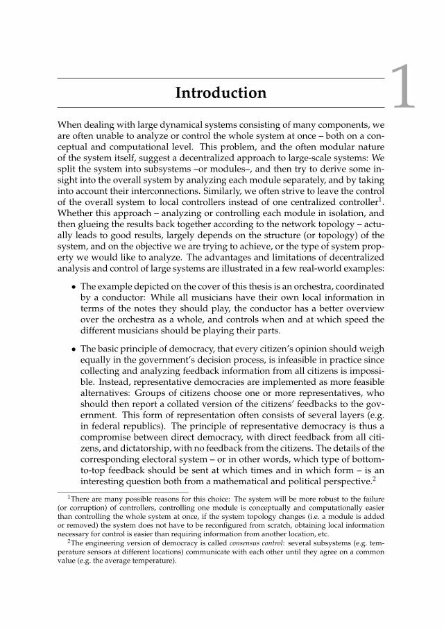
Introduction 1When dealing with large dynamical systems consisting of many components, weare often unable to analyze or control the whole system at once – both on a con-ceptual and computational level. This problem, and the often modular natureof the system itself, suggest a decentralized approach to large-scale systems: Wesplit the system into subsystems –or modules–, and then try to derive some in-sight into the overall system by analyzing each module separately, and by takinginto account their interconnections. Similarly, we often strive to leave the controlof the overall system to local controllers instead of one centralized controller1.Whether this approach – analyzing or controlling each module in isolation, andthen glueing the results back together according to the network topology – actu-ally leads to good results, largely depends on the structure (or topology) of thesystem, and on the objective we are trying to achieve, or the type of system prop-erty we would like to analyze. The advantages and limitations of decentralizedanalysis and control of large systems are illustrated in a few real-world examples:
• The example depicted on the cover of this thesis is an orchestra, coordinatedby a conductor: While all musicians have their own local information interms of the notes they should play, the conductor has a better overviewover the orchestra as a whole, and controls when and at which speed thedifferent musicians should be playing their parts.
• The basic principle of democracy, that every citizen’s opinion should weighequally in the government’s decision process, is infeasible in practice sincecollecting and analyzing feedback information from all citizens is impossi-ble. Instead, representative democracies are implemented as more feasiblealternatives: Groups of citizens choose one or more representatives, whoshould then report a collated version of the citizens’ feedbacks to the gov-ernment. This form of representation often consists of several layers (e.g.in federal republics). The principle of representative democracy is thus acompromise between direct democracy, with direct feedback from all citi-zens, and dictatorship, with no feedback from the citizens. The details of thecorresponding electoral system – or in other words, which type of bottom-to-top feedback should be sent at which times and in which form – is aninteresting question both from a mathematical and political perspective.2
1There are many possible reasons for this choice: The system will be more robust to the failure(or corruption) of controllers, controlling one module is conceptually and computationally easierthan controlling the whole system at once, if the system topology changes (i.e. a module is addedor removed) the system does not have to be reconfigured from scratch, obtaining local informationnecessary for control is easier than requiring information from another location, etc.
2The engineering version of democracy is called consensus control: several subsystems (e.g. tem-perature sensors at different locations) communicate with each other until they agree on a commonvalue (e.g. the average temperature).
2 Chapter 1: Introduction
• In contrast to the democratic structure based on feedback through voting,hierarchical personnel structures with little or no bottom-to-top feedbackare very common in organizations – traditionally in the army, but also inmany companies. In this type of structures, control of the overall system isbased on the chain-of-command principle, allowing the top of the hierar-chy to better control and predict the state of the overall system, and facili-tating quick responses to changing conditions since no consensus needs tobe found. While typically undesirable for humans, its efficiency makes thisstructure a useful topology for decentralized engineering systems.
• The human body – as well as many other biological entities – is an inher-ently modular system: In a nutshell, it is an interconnection of several or-gans, each with its own limited task and functionality. These modules areinterconnected by the nerve system, and controlled partly via a central con-troller (the brain) and partly via local controllers (e.g. local reflexes). Onlythrough the coordination of these different modules is it possible to achievecomplex tasks, such as playing tennis, which none of the modules couldachieve independently.
• Another example for a decentralized system in which some form of coordi-nation is inevitable is traffic: Each car is an independent entity, with its ownobjective (to reach a destination) and its own local controller (the driver us-ing the gas pedal and steering wheel). These entities are interconnected bythe fact that two cars should never be at the same place at the same time(i.e. vehicles should not collide). This consideration gave rise to controlmeasures such as traffic lights, which coordinate the different cars passingthrough the same intersection. Moreover, different traffic lights along thesame major road often cooperate to allow for green waves, while trafficlights in different parts of the country are independent of each other.
From these examples, we can already derive some basic principles about decen-tralized control:
• decentralization – i.e. splitting the system into parts and controlling eachpart locally – is usually desirable but not always possible,
• hierarchies naturally arise from practicalities, and are often preferable toother types of system structures,
• in decentralized control, it is essential where information is available, andhow (i.e. at which location) we can exert control on the system.
The aim of this thesis is to contribute to the mathematical formalization and ex-ploration of some of these principles.
1.1 Introduction to coordination control 3
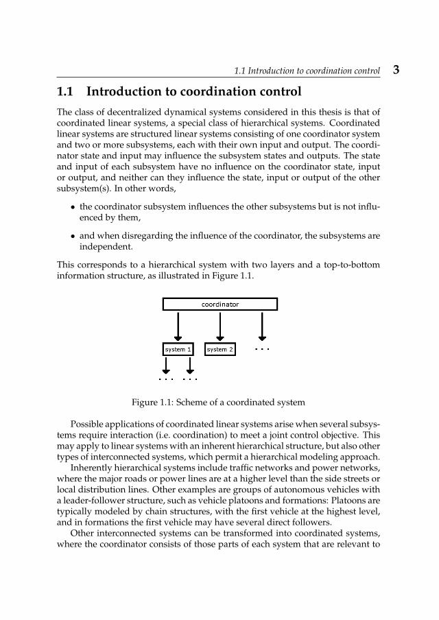
1.1 Introduction to coordination controlThe class of decentralized dynamical systems considered in this thesis is that ofcoordinated linear systems, a special class of hierarchical systems. Coordinatedlinear systems are structured linear systems consisting of one coordinator systemand two or more subsystems, each with their own input and output. The coordi-nator state and input may influence the subsystem states and outputs. The stateand input of each subsystem have no influence on the coordinator state, inputor output, and neither can they influence the state, input or output of the othersubsystem(s). In other words,
• the coordinator subsystem influences the other subsystems but is not influ-enced by them,
• and when disregarding the influence of the coordinator, the subsystems areindependent.
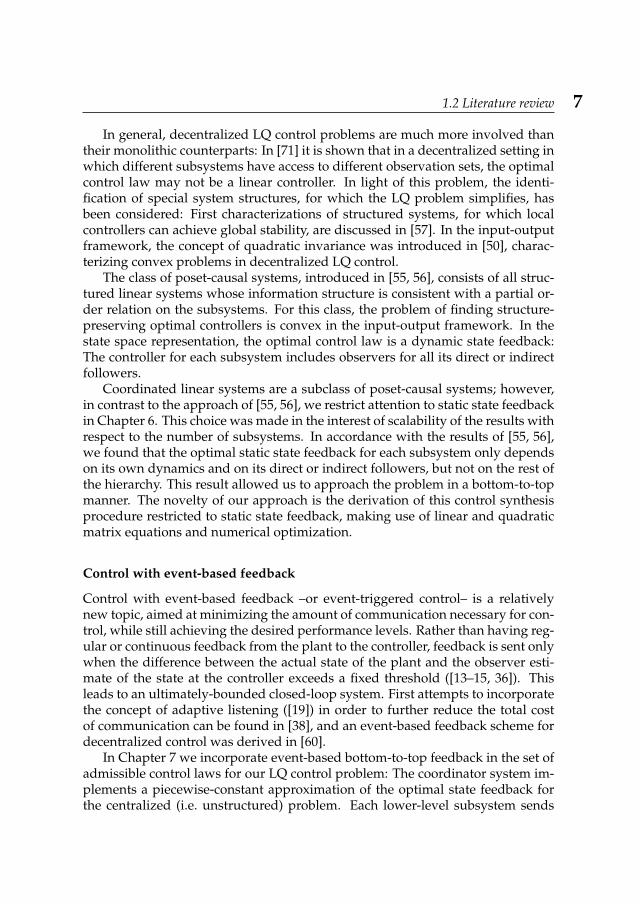
This corresponds to a hierarchical system with two layers and a top-to-bottominformation structure, as illustrated in Figure 1.1.
Figure 1.1: Scheme of a coordinated system
Possible applications of coordinated linear systems arise when several subsys-tems require interaction (i.e. coordination) to meet a joint control objective. Thismay apply to linear systems with an inherent hierarchical structure, but also othertypes of interconnected systems, which permit a hierarchical modeling approach.
Inherently hierarchical systems include traffic networks and power networks,where the major roads or power lines are at a higher level than the side streets orlocal distribution lines. Other examples are groups of autonomous vehicles witha leader-follower structure, such as vehicle platoons and formations: Platoons aretypically modeled by chain structures, with the first vehicle at the highest level,and in formations the first vehicle may have several direct followers.
Other interconnected systems can be transformed into coordinated systems,where the coordinator consists of those parts of each system that are relevant to
4 Chapter 1: Introduction
the other systems, and the subsystems consist of the remaining parts of each sys-tem. This corresponds to imposing a hierarchy on the different parts of a decen-tralized system, in order to facilitate decentralized control synthesis. Moreover,large-scale monolithic systems can be decomposed into subsystems with a hier-archical information structure in order to reduce the computational effort neededfor control synthesis.3
This thesis develops an in-depth mathematical analysis of coordinated linearsystems, focusing on the following questions:
(1) How can we construct coordinated linear systems, from large monolithicsystems or decentralized systems with non-hierarchical information struc-tures (e.g. interconnected systems with two-way communication)?
(2) Given a coordinated linear system, is this system ‘as decentralized as pos-sible’, i.e. are all interactions allowed by the system structure actually re-quired? Is all communication actually necessary? And can centralized mea-surement or control actions be replaced by local ones?
(3) Which part of each subsystem is controllable by which input – can controlbe done locally, or is coordination required to meet the control objective?
(4) A similar question arises for observability: Is all measurement data whichis necessary for implementing a given control law available locally, or iscommunication of measurement data required?
(5) Given a coordinated linear system and an achievable control objective, howcan we synthesize a control law which achieves this control objective, butalso respects the given information structure? How does the performance ofsuch a control law compare to its centralized counterpart? Will performanceimprove if bottom-to-top communication is permitted on an event-drivenbasis?
(6) Can we extend concepts and results derived for coordinated linear systemsto related classes of coordinated and hierarchical systems?
1.2 Literature reviewConcerning questions (1)-(6) above, this section summarizes some of the previouswork, and relates it to the contributions of this thesis.
3Other criteria for the decomposition of dynamical systems into several parts include geographicalproximity and different time scales in the system evolution.
1.2 Literature review 5
System decompositions
Most previous work on decompositions of linear systems is based on structuredmatrices and graph-theoretic approaches ([9, 57]): The system matrices are re-duced to binary (structured) form, for each entry specifying whether it is zeroor non-zero. The dependencies among the different state, input and output vari-ables can then be represented by a directed graph, with the different variablesas nodes, and directed edges among them whenever the corresponding entriesin the structured system matrices are non-zero. The graph-theoretic concepts ofreachability and co-reachability can then be used to decompose the system, andto analyze the interconnections among the subsystems. A major drawback of thisapproach is that it ignores the different possible structures corresponding to agiven linear system under transformed state, input and output spaces.
A complementary approach for decomposing large linear systems is basedon the strength of the interactions among the different subsystems: Weak inter-actions are identified e.g. via dissipation inequalities ([1]), and then removed,leading to a more decentralized approximation of the original system. Other de-composition approaches are based on different time scales, different geographicregions, etc. ([5]).
Previous work on the special case of decompositions into hierarchical linearsystems includes decompositions based on aggregation ([34, 43]): Lower-orderapproximations of the original system (or subsystems) are used on the higherlevel, in order to reduce the complexity of the control synthesis procedure. Ageometric approach to coordination control, in which a system is decomposedusing feedback compensation, can be found in [64]. The goal of this decompo-sition is to identify a coordinator and several subsystems, with the coordinatorcontrolling the system-wide performance, while the subsystems do local control.The compensating feedback is chosen such that system becomes a hierarchicalsystem.
The approach used in Chapter 4 of this thesis differs from existing approachesin the sense that it uses the geometric (i.e. basis-independent) concepts of con-trollability and observability subspaces, and that the original system and inter-connections are neither changed nor aggregated, and the option of having com-pensating feedback is not taken into account. Another original contribution ofChapter 4 is the development of concepts and results concerning the minimalityof a given decomposition.
In the related field of team theory, the decomposition of a linear system ac-cording to the observations and influence of two independent decision makerswas studied in [51] – this is a special case of the decomposition derived in Section4.3.4.
6 Chapter 1: Introduction
Controllability and observability
While the classical concepts of controllability and observability ([21]) for unstruc-tured systems are characterized in terms of invariant subspaces of the state space,most literature on controllability and observability in decentralized settings isbased on graph-theoretic concepts: A system is called structurally controllableif every state variable is reachable from at least one input variable in the corre-sponding graph representation ([8, 9, 57]). Structural controllability is a basis-dependent concept, and it is necessary, but in general not sufficient for controlla-bility. The dual concept is structural observability, defined via the co-reachabilityof the state variables from at least one output variable. In [35], driver nodes areidentified, which can control the whole network (given as linear system).
Early work in the field of team theory discusses the controllability and observ-ability of a linear system via multiple decision makers with partial observations([2, 16]), using invariant subspaces of the state space. In Chapter 5, this approachis generalized to coordinated linear systems. Together with the novel distinctionbetween independently and jointly reachable subspaces, and between completelyand independently indistinguishable subspaces, this allowed for a systematic ap-proach to the problem of defining concepts of controllability and observabilityfor coordinated linear systems.
LQ optimal control
For monolithic systems, the LQ control problem was introduced and solved in[20]. Early decentralized versions of the LQ problem appeared in the field ofteam theory (a subfield of game theory), where several decision makers, eachwith partial observations of the state of a linear system, aim at minimizing a jointquadratic control objective ([2, 16, 45]). Team theory problems with delayed com-munication among the decision makers are discussed in [49]. A different setup isthat of Stackelberg games (also stemming from game theory), where the decisionmakers are one leader and one follower: First the leader makes a control decision,and then the follower bases its control decision on information about the leader’sdecision ([17, 68]).
In the field of control theory, early work on decentralized control methods forlarge scale and hierarchical systems is surveyed in [52], and an early survey ofleader-follower strategies is given in [6]. A linear-quadratic coordination controlproblem was described in [3]. In this setup, the aspect of coordination was notrelated to the information structure, but to the control objective: The coordinatorminimizes a global control objective, taking into account the subsystem controllaws, and the subsystems minimize local control objectives. Local or structuredcontrol feedback synthesis for decentralized LQ control problems was also dis-cussed in [58], [57] and [53].
1.2 Literature review 7
In general, decentralized LQ control problems are much more involved thantheir monolithic counterparts: In [71] it is shown that in a decentralized setting inwhich different subsystems have access to different observation sets, the optimalcontrol law may not be a linear controller. In light of this problem, the identi-fication of special system structures, for which the LQ problem simplifies, hasbeen considered: First characterizations of structured systems, for which localcontrollers can achieve global stability, are discussed in [57]. In the input-outputframework, the concept of quadratic invariance was introduced in [50], charac-terizing convex problems in decentralized LQ control.
The class of poset-causal systems, introduced in [55, 56], consists of all struc-tured linear systems whose information structure is consistent with a partial or-der relation on the subsystems. For this class, the problem of finding structure-preserving optimal controllers is convex in the input-output framework. In thestate space representation, the optimal control law is a dynamic state feedback:The controller for each subsystem includes observers for all its direct or indirectfollowers.
Coordinated linear systems are a subclass of poset-causal systems; however,in contrast to the approach of [55, 56], we restrict attention to static state feedbackin Chapter 6. This choice was made in the interest of scalability of the results withrespect to the number of subsystems. In accordance with the results of [55, 56],we found that the optimal static state feedback for each subsystem only dependson its own dynamics and on its direct or indirect followers, but not on the rest ofthe hierarchy. This result allowed us to approach the problem in a bottom-to-topmanner. The novelty of our approach is the derivation of this control synthesisprocedure restricted to static state feedback, making use of linear and quadraticmatrix equations and numerical optimization.
Control with event-based feedback
Control with event-based feedback –or event-triggered control– is a relativelynew topic, aimed at minimizing the amount of communication necessary for con-trol, while still achieving the desired performance levels. Rather than having reg-ular or continuous feedback from the plant to the controller, feedback is sent onlywhen the difference between the actual state of the plant and the observer esti-mate of the state at the controller exceeds a fixed threshold ([13–15, 36]). Thisleads to an ultimately-bounded closed-loop system. First attempts to incorporatethe concept of adaptive listening ([19]) in order to further reduce the total costof communication can be found in [38], and an event-based feedback scheme fordecentralized control was derived in [60].
In Chapter 7 we incorporate event-based bottom-to-top feedback in the set ofadmissible control laws for our LQ control problem: The coordinator system im-plements a piecewise-constant approximation of the optimal state feedback forthe centralized (i.e. unstructured) problem. Each lower-level subsystem sends
8 Chapter 1: Introduction
its current state to the coordinator whenever the approximation error, caused byusing the last communicated value instead of the current value of the subsys-tem state at the coordinator level, exceeds a certain threshold. Novelties of thisapproach are the use of an exponentially decaying threshold, which leads to anexponentially stable closed-loop system, and bounding the approximation errorinstead of the difference between the current and last received state.
1.3 Contents of the thesisThis thesis is structured as follows:
As prerequisite material, some elements of the classical theory of linear sys-tems are summarized in Chapter 2. In Chapter 3, the concept of a coordinated lin-ear system is defined and characterized, several basic properties of coordinatedlinear systems are derived, and an overview of related decentralized systems isgiven.
Chapter 4 deals with questions (1) and (2): In Section 4.1 we give some con-struction procedures for the transformation of monolithic and interconnected lin-ear systems into coordinated linear systems. Based on the considerations sum-marized in question (2), several concepts of minimality of a given coordinatedlinear system decomposition are introduced and characterized in Section 4.2, andsome results concerning the construction of a minimal decomposition are given.
Questions (3) and (4) are discussed in Chapter 5: In Section 5.2, the concept ofreachability is refined to distinguish among the different inputs and the differentparts of the overall system state, and based on this, a controllability decomposi-tion for coordinated linear systems is derived, and several different concepts ofcontrollability are defined and characterized. A similar approach is used for theconcepts of indistinguishability and observability in Section 5.3. We then illus-trate how to combine these concepts, and derive equivalent conditions for stabi-lizability via dynamic measurement feedback.
While question (5), in the generality in which it is formulated above, is eas-ier posed than answered, its restriction to LQ control problems is the topic ofChapters 6 and 7: The LQ problem over all structure-preserving static state feed-backs is discussed in Chapter 6. The overall control problem is separated intoconditionally independent subproblems, a numerical approach to their solutionis derived, and the behavior and performance of the resulting control law areillustrated in examples. Chapter 7 focuses on the last part of question (5): We ap-proximate the centralized (i.e. not structure-preserving) optimum by introducingevent-based bottom-to-top feedback, and derive bounds on the stability of theresulting closed-loop system and on the corresponding costs.
As an illustration of the theory developed in this thesis and its potential practi-cal purposes, Chapter 8 discusses two case studies of coordination control: In Sec-tion 8.1, a formation flying problem for autonomous underwater vehicles (AUVs)
1.3 Contents of the thesis 9
is introduced and solved using the coordination control framework developed inthe previous chapters. Section 8.2 deals with coordinated ramp metering, i.e. thecoordinated control of on-ramp metering devices at two neighboring on-rampsof a highway.
Chapter 9 summarizes the main results of this thesis, and points to some pos-sible directions of extending the results to related classes of systems, as suggestedin question (6).

10 Chapter 1: Introduction
Prerequisites 2In this chapter, some elements of the classical theory of monolithic (i.e. unstruc-tured) linear systems are summarized as background material necessary for thelater chapters.
2.1 NotationThe notation for system-theoretic concepts used in this thesis complies in largeparts with e.g. [63]. The direct sum of two independent linear spaces will bedenoted by +, i.e.
V +W =
[vw
]∣∣∣∣ v ∈ V, w ∈W =
[I0
]V +
[0I
]W.
For notational simplicity, we restrict attention to coordinated linear systemswith one coordinator and two subsystems. The two subsystems are indexed by 1and 2, and the coordinator is indexed by c. The index i is used for the subsystemsonly (i.e. i = 1, 2), and the index j denotes all three parts of the system (i.e. j =1, 2, c). State spaces are denoted by X , input spaces by U , and output spaces byY . Their dimensions are denoted by n = dimX, m = dimU and p = dimY .
The state, input and output space of a coordinated linear system are composedof the state, input and output spaces of the subsystems and coordinator, i.e.
X = X1+X2+Xc, U = U1+U2+Uc, Y = Y1+Y2+Yc,
with dimensions n1 + n2 + nc = n, m1 + m2 + mc = m and p1 + p2 + pc = p.Note that throughout this thesis, we will use the notation X1 both for the
linear space X1 of dimension n1, and for the n1-dimensional linear subspace ofthe n-dimensional space X . In other words, we use the notation X1 both for
the space itself and for its natural embedding
I00
X1 into X = X1+X2+Xc. In
particular, for M ∈ Rn×n and S a linear subspace of X , we use the notation MX1
for the image space M
I00
X1 ⊆ X , and the notation X1 ∩ S for the intersection
space
I00
X1
∩ S ⊆I0
0
X1. The same holds for the spaces X2 and Xc and
12 Chapter 2: Prerequisites
their embeddings
0I0
X2 and
00I
Xc into X , and for the corresponding input
and output spaces.The state, input and output of a coordinated linear systems are then denoted
by
x(t) =
x1(t)x2(t)xc(t)
, u(t) =
u1(t)u2(t)uc(t)
and y(t) =
y1(t)y2(t)yc(t)
.In some parts of this thesis, we restrict attention to one subsystem and one co-ordinator, in which case the subsystem is indexed by s, and the state, input andoutput vectors are denoted by
x(t) =
[xs(t)xc(t)
], u(t) =
[us(t)uc(t)
]and y(t) =
[ys(t)yc(t)
].
2.2 Monolithic linear systemsThe following sections summarize some of the theory for linear time-invariantsystems that will be needed in the following chapters. We primarily work withcontinuous-time systems, but some examples and simulations use the discrete-time equivalent. Here we consider the class of all linear systems of the form
x(t) = Ax(t) + Bu(t),
y(t) = Cx(t),(2.1)
with state space X , input space U and output space Y , and with initial statex(0) = x0. If the input trajectory u : [0, t]→ U is a piecewise-continuous functionthen the integral on the right hand side of (2.2) is well-defined as a Riemannintegral, and the state x(t) at time t is then given by
x(t) = eAtx0 +
∫ t
0
eA(t−τ)Bu(τ)dτ. (2.2)
The output y(t) is given by
y(t) = Cx(t) = CeAtx0 +
∫ t
0
CeA(t−τ)Bu(τ)dτ.
2.3 Controllability and observability 13
Taking the Laplace transform, we get the input-output relation
y(s) = G(s)u(s), s ∈ C
in the frequency domain, with transfer function
G(s) = C(sI −A)−1B.
The transfer function is a rational matrix function, which characterizes the input-output behavior of a continuous-time linear system without the need of a statevariable, and hence independently of the choice of the state space and its basis.
2.3 Controllability and observabilityFor linear systems, the concepts of reachability and controllability are defined asfollows (see e.g. [63]):
A state x ∈ X is called reachable (from the initial state x0 = 0) if thereexists a finite terminal time t < ∞ and a piecewise-continuous in-put trajectory u : [0, t] → U such that the state trajectory of thelinear system with x0 = 0 satisfies x(t) = x. The set of all reach-able states will be denoted by R. A linear system (or, equivalently,the matrix pair (A,B)) is called controllable if X = R.
The reachable set R is the smallestA-invariant subspace ofX containing im B,see [63, 72]. This subspace is unique, and is given by
R = im[B AB A2B . . . An−1B
], (2.3)
where n is the state space dimension dimX . The matrix[B AB . . . An−1B
]is called the controllability matrix. Observe that R is an A-invariant subspace bythe Cayley-Hamilton theorem.
From these properties, we can derive the Kalman controllability decomposi-tion (see e.g. [21]): Let X1 = R, and choose for X2 any complement of X1 in X ,then with respect to the decomposition X = X1+X2 the system has the form
x(t) =
[A11 A12
0 A22
]x(t) +
[B1
0
]u(t),
y(t) =[C1 C2
]x(t).
(2.4)
The matrix pair (A11, B1) is a controllable pair.
14 Chapter 2: Prerequisites
We call a matrixM ∈ Rn×n exponentially stable if its spectrum lies in the openleft half plane, i.e. if σ(M) ⊂ C− = z ∈ C | Re(z) < 0. The related concept ofstabilizability is then defined as follows:
A linear system (or, equivalently, the matrix pair (A,B)) is called sta-bilizable if there exists a linear state feedback F ∈ Rm×n such thatthe closed-loop system x(t) = (A+BF )x(t), obtained by applyingthe input u(t) = Fx(t), is stable.
Stabilizability is equivalent to the matrix A22 in (2.4) being a stable matrix. Theexponential of a stable matrix is bounded in norm by a negative scalar exponen-tial, i.e.
M stable =⇒ ∃ α > 0, c ∈ R s.t.∥∥eMt
∥∥ ≤ ce−αt ∀t ∈ R.Applying the stabilizing state feedback u(·) = Fx(·) leads to the closed-loop statetrajectory x(t) = e(A+BF )tx0, satisfying
‖x(t)‖ =∥∥∥e(A+BF )tx0
∥∥∥ ≤ ∥∥∥e(A+BF )t∥∥∥ ‖x0‖ ≤ ce−αt ‖x0‖ .
Hence the closed-loop state trajectory goes to zero exponentially for t→∞.
The concepts of indistinguishability and observability are typically defined asfollows (see e.g. [63]):
A pair (x, ¯x) of states in X is called indistinguishable if the outputsy(t) and ¯y(t), generated by the linear system with input trajectoryu ≡ 0 and initial conditions x0 = x and x0 = ¯x, respectively, havey(t) = ¯y(t) for all t ∈ [0,∞). The set of all states x ∈ X suchthat (x, 0) is indistinguishable will be called I. A linear system(or, equivalently, the matrix pair (C,A)) is called observable if I =0.
Note that for linear systems, the pair (x, ¯x) is indistinguishable if and only ifthe pair (x − ¯x, 0) is indistinguishable. Hence, when studying the observabilityproperties of linear systems, we can restrict attention to pairs of the form (x, 0).In the following, and with some abuse of notation, a state x ∈ X will be called in-distinguishable if the pair (x, 0) is indistinguishable in the sense defined above.
The set of indistinguishable states I is the largest A-invariant subspace of Xcontained in kerC, see [63, 72]. This subspace is unique, and is given by
I = ker
CCACA2
...CAn−1
, (2.5)
2.4 LQ optimal control 15
with n = dimX . The matrix
CCA
...CAn−1
is called the observability matrix. A-
invariance of I again follows from the Cayley-Hamilton theorem.The A-invariance property leads to the Kalman observability decomposition
(see e.g. [21]): Let X2 = I and choose for X1 any complement of X2 in X , thenwith respect to the decomposition X = X1+X2, the system has the form
x(t) =
[A11 0A21 A22
]x(t) +
[B1
B2
]u(t),
y(t) =[C1 0
]x(t).
(2.6)
The pair (C1, A11) is an observable pair.In analogy to stabilizability, the concept of detectability is defined as follows:
A linear system (or, equivalently, the matrix pair (C,A)) is called de-tectable if there exists a linear state observer matrixK ∈ Rn×p suchthat the system describing the observer error e(t) = (A −KC)e(t)is stable.
Detectability is equivalent to the matrix A22 in (2.6) being a stable matrix.
2.4 LQ optimal controlWe consider unstructured linear time-invariant deterministic systems. Theinfinite-horizon, undiscounted linear-quadratic (LQ) control problem is given by
minu(·) piecewise continuous
J(x0, u(·)), (2.7)
with cost function
J(x0, u(·)) =
∫ ∞t0
xT (t)Qx(t) + uT (t)Ru(t) dt, (2.8)
subject to the system dynamics
x(t) = Ax(t) + Bu(t), x(t0) = x0. (2.9)
If Q ≥ 0 and R > 0 then the problem is a well-defined minimization problem, i.e.there exists a piecewise continuous u(·) such that the minimum is attained.
16 Chapter 2: Prerequisites
In other words, our control objective in LQ optimal control is to minimize aquadratic cost function, representing a trade-off: The cost function penalizes theweighted norm of the state trajectory on the one hand, and the weighted norm ofthe control effort on the other hand.
The solution of this problem is well-known (see e.g. [63]): If (A,B) is a stabi-lizable pair and (Q,A) is a detectable pair then the algebraic Riccati equation
XBR−1BTX −ATX −XA −Q = 0 (2.10)
has a unique solution X such that A − BR−1BTX is stable. This solution X isalso the largest positive semidefinite solution. The optimal control law is thenthe state feedback u(·) = Gx(·), where G = −R−1BTX . The closed-loop system isgiven by
x(t) = (A + BG)x(t) = (A −BR−1BTX)x(t),
with A−BR−1BTX stable by the choice of X . The corresponding cost is given by
J(x0, Gx(·)) = xT0 Xx0. (2.11)
The control law u(·) = Gx(·) derived above has the following properties:
• the optimal input trajectory is a linear state feedback, i.e. it is of the formu(t) = Gx(t) where G is a matrix and x(t) is the current state,
• the feedback matrix G is independent of the initial state x0,
• the entries of G, and also the corresponding cost J(x0, Gx(·)), can be com-puted offline.
In Chapter 6, we will derive the corresponding results for the case of coordinatedlinear systems, and compare the properties of the coordination control law withthe properties given here.
2.4.1 Relation between costs and control lawsThe following result quantifies the relative cost increase caused by using otherstate feedbacks than the optimal one, and will be useful in Chapter 6, when werestrict the set of admissible feedback matrices to those respecting the underlyinginformation structure.
This theorem is a slight variation of Lemma 16.3.2 in [33], and a proof is givenfor convenience:
2.4.1. Theorem. We consider a system of the form (2.9) and the optimal control problem(2.7), with cost function (2.8). We assume that Q ≥ 0, R > 0, (A,B) is a stabilizablepair, and (Q,A) is a detectable pair. Let X be the stabilizing solution of (2.10), and let
2.4 LQ optimal control 17
G = −R−1BTX . For any other stabilizing state feedback matrix F the difference in costis given by
J(x0, Fx(·)) − J(x0, Gx(·)) =
∫ ∞0
‖R1/2(F −G)e(A+BF )tx0‖2dt.
Proof. We have J(x0, Gx(·)) = xT0 Xx0. The cost corresponding to any other sta-bilizing feedback F is given by the solution Y of the Lyapunov equation
(A + BF )TY + Y (A + BF ) + FTRF + Q = 0 :
For this choice of Y , and noting that limt→∞ e(A+BF )t = 0, we have
J(x0, Fx(·)) =
∫ ∞0
x(t)T (Q + FTRF )x(t) dt
=
∫ ∞0
−x(t)T ((A + BF )TY + Y (A + BF ))x(t) dt
= xT0
∫ ∞0
−d
dt
(e(A+BF )T tY e(A+BF )t
)dt x0
= xT0
(− e(A+BF )T tY e(A+BF )t
∣∣∣t→∞
+ e(A+BF )T tY e(A+BF )t∣∣∣t=0
)x0 = xT0 Y x0.
In the following, we derive a Lyapunov equation for the difference Y −X of thecosts, using the Riccati equation for X and the Lyapunov equation for Y :
(A + BF )T (Y −X) + (Y −X)(A + BF )
= −FTRF −Q −ATX − FTBTX −XA −XBF
= −FTRF −XBR−1BTX − FTBTX −XBF
= −(F + R−1BTX)TR(F + R−1BTX)
= −(F −G)TR(F −G).
Using this, we can now derive an expression for the cost difference:
J(x0, Fx(·)) − J(x0, Gx(·)) = xT0 (Y −X)x0
= xT0
∫ ∞0
−d
dt
(e(A+BF )T t(Y −X)e(A+BF )t
)dt x0
= xT0
∫ ∞0
−(e(A+BF )T t((A + BF )(Y −X) + (Y −X)(A + BF ))e(A+BF )t
)dt x0
18 Chapter 2: Prerequisites
= xT0
∫ ∞0
(e(A+BF )T t(F −G)TR(F −G)e(A+BF )t
)dt x0
=
∫ ∞0
‖R1/2(F −G)xF (t)‖2dt,
where xF (·) is the state trajectory of the closed-loop system obtained from apply-ing the feedback Fx(·), i.e. xF (t) = e(A+BF )tx0.
From the theorem above we see that the difference in cost between the optimalsolution and another stabilizing solution can be described in terms of the corre-sponding feedback matrices. If no special restrictions are imposed on the feed-back F considered here, then minimizing xT0 (Y −X)x0 trivially leads to F = G,with Y = X .
However, in decentralized control it is often necessary, or preferable, that Fcomplies with the underlying information structure of the system. Our resultabove states that for any non-empty subset F ⊆ F ∈ Rm×n|σ(A + BF ) ⊂ C− ,the problem
infF∈F
xT0 Y x0
has a solution (if the unrestricted problem has a solution, i.e. if X exists), and thissolution can be found by solving
infF∈F
∫ ∞0
‖R1/2(F −G)xF (t)‖2dt,
or equivalently
infF∈F
∫ ∞0
‖R1/2(F −G)e(A+BF )tx0‖2dt.
Coordinated Linear Systems 3An intuitive description of coordinated linear systems was given in Section 1.1.In the following, coordinated linear systems will be defined, and several of theirbasic properties will be discussed.
3.1 DefinitionFor the purposes of this thesis, and in contrast to [48], we define coordinated lin-ear systems with inputs and outputs in terms of independence and invarianceproperties of the state, input and output spaces. This geometric approach to lin-ear systems was developed in [72].
3.1.1. Definition. Let a continuous-time, time-invariant linear system with in-puts and outputs, of the form
x(t) = Ax(t) + Bu(t),
y(t) = Cx(t)
be given. Moreover, let the state space, input space and output space of the sys-tem be decomposed as
X = X1+X2+Xc, U = U1+U2+Uc and Y = Y1+Y2+Yc.
Then we call the system a coordinated linear system if we have that
(1) X1 and X2 are A-invariant,1
(2) BU1 ⊆ X1 and BU2 ⊆ X2,
(3) and CX1 ⊆ Y1 and CX2 ⊆ Y2.
In this definition, the subspaces Xc, Uc and Yc are the state, input and outputspaces of the coordinator system, the subspaces X1, U1 and Y1 correspond tosubsystem 1, and the subspaces X2, U2 and Y2 correspond to subsystem 2. Con-ditions (1), (2) and (3) in Definition 3.1.1 imply that the state and input of eachsubsystem have no influence on the states or the outputs of the coordinator orthe other subsystem.
With respect to the decompositions X = X1+X2+Xc, U = U1+U2+Uc andY = Y1+Y2+Yc, the system is then of the form
1Note that we use X1 to denote both the space X1 and the subspace
I00
X1 ⊆ X (see Section 2.1).
20 Chapter 3: Coordinated Linear Systems
x(t) =
A11 0 A1c
0 A22 A2c
0 0 Acc
x(t) +
B11 0 B1c
0 B22 B2c
0 0 Bcc
u(t),
y(t) =
C11 0 C1c
0 C22 C2c
0 0 Ccc
x(t).
(3.1)
The structure of the system matrices in (3.1) follows directly from Conditions (1),(2) and (3) in Definition 3.1.1. Note that, with the trivial choices
X1 = 0, X2 = 0, Xc = X,U1 = 0, U2 = 0, Uc = U,Y1 = 0, Y2 = 0, Yc = Y,
any linear system qualifies as a coordinated linear system.The interconnections between the different variables of a coordinated linear
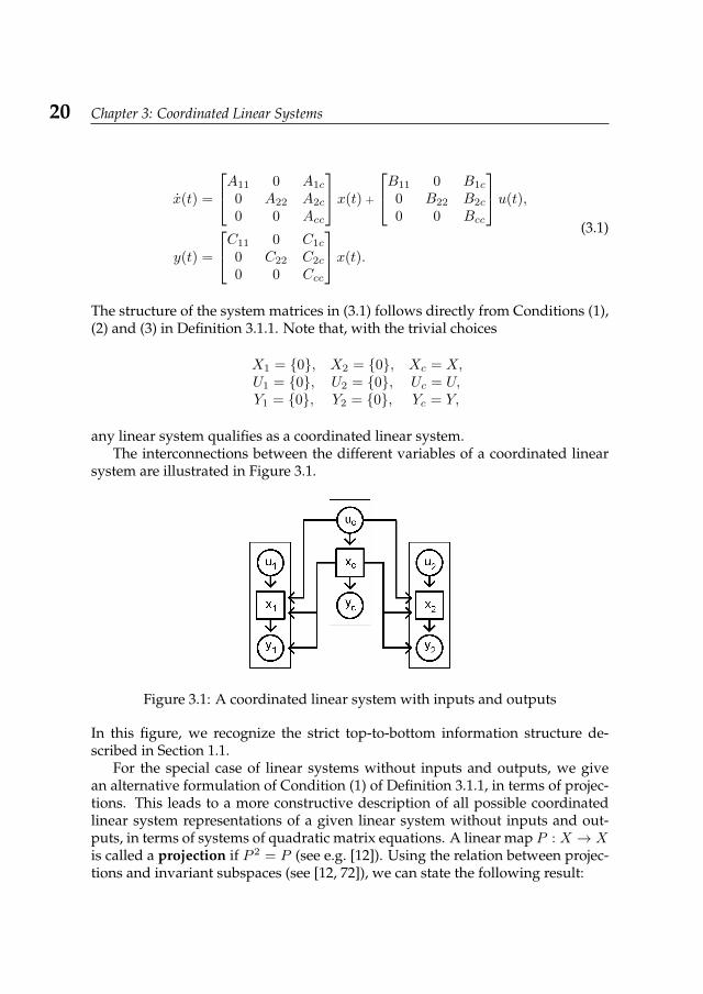
system are illustrated in Figure 3.1.
Figure 3.1: A coordinated linear system with inputs and outputs
In this figure, we recognize the strict top-to-bottom information structure de-scribed in Section 1.1.
For the special case of linear systems without inputs and outputs, we givean alternative formulation of Condition (1) of Definition 3.1.1, in terms of projec-tions. This leads to a more constructive description of all possible coordinatedlinear system representations of a given linear system without inputs and out-puts, in terms of systems of quadratic matrix equations. A linear map P : X → Xis called a projection if P 2 = P (see e.g. [12]). Using the relation between projec-tions and invariant subspaces (see [12, 72]), we can state the following result:
3.2 Basic properties 21
3.1.2. Proposition. For the projections P1 : X → X and P2 : X → X , the linearsubspaces X1 = P1X and X2 = P2X of X are independent and satisfy Condition (1) ofDefinition 3.1.1, if and only if P1 and P2 satisfy
P1AP1 = AP1, P2AP2 = AP2, (3.2)P1P2 = 0, P2P1 = 0. (3.3)
Proof. This follows directly from the fact that a subspace S of X is A-invariant ifand only if PAP = AP for some (and equivalently, any) projector P : X → Xwith imP = S. Condition (3.3) is equivalent to
X1 ∩X2 = P1X ∩ P2X = 0.
Extending Proposition 3.1.2 to linear systems with inputs and outputs is con-ceptually straightforward but notationally more involved.
3.2 Basic propertiesThe set of matrices
RCLS =
M11 0 M1c
0 M22 M2c
0 0 Mcc
, Mij ∈ Rni×nj , i, j = 1, 2, c
forms an invertible algebraic ring (i.e. it is closed with respect to taking linearcombinations, matrix multiplication, and matrix inversion):linear combinations:
α
A11 0 A1c
0 A22 A2c
0 0 Acc
+β
B11 0 B1c
0 B22 B2c
0 0 Bcc
=
αA11+βB11 0 αA1c+βB1c
0 αA22+βB22 αA2c+βB2c
0 0 αAcc+βBcc
.matrix multiplication:A11 0 A1c
0 A22 A2c
0 0 Acc
B11 0 B1c
0 B22 B2c
0 0 Bcc
=
A11B11 0 A11B1c + A1cBcc0 A22B22 A22B2c + A2cBcc0 0 AccBcc
.
22 Chapter 3: Coordinated Linear Systems
matrix inversion: Suppose M ∈ RCLS is invertible, then M11,M22,Mcc are invert-ible because M is block upper-triangular. M−1 is given by
M−1 =
M−111 0 −M−1
11M1cM−1cc
0 M−122 −M−1
22M2cM−1cc
0 0 M−1cc
∈ RCLS
In particular, eM is of the form
exp
M11 0 M1c
0 M22 M2c
0 0 Mcc
=
eM11 0 ?1c
0 eM22 ?2c
0 0 eMcc
, (3.4)
where the entries denoted by ? are not specified further. Hence the informa-tion structure imposed by the invariance properties of Definition 3.1.1 is left un-changed over time by the system dynamics.
A natural consequence of this invariance property is that the transfer functionis of the form
G(z) = C(zI −A)−1B
=
C11(zI −A11)−1B11 0 ?1c
0 C22(zI −A22)−1B22 ?2c
0 0 Ccc(zI −Acc)−1Bcc
,where
?ic = Cii(zI −Aii)−1Bic + (Cic − Cii(zI −Aii)
−1Aic)(zI −Acc)−1Bcc.
Note that the diagonal entries of the linear combination, product and inverseare just the linear combination, product and inverse of the corresponding diago-nal entries of the original matrices, respectively. This means that these operationsalso preserve the structure of matrices corresponding to more nested hierarchies:If A ∈ RCLS with a diagonal entry Aii ∈ RCLS, then operations as above will yieldmatrices in RCLS with the ii-th entry again in RCLS.
Hence coordinated linear systems can act as building blocks for constructinglinear systems with a more complex hierarchical structure: An extension to anarbitrary number of subsystems is straightforward, and nested hierarchies can bemodeled by using another coordinated linear system as one of the subsystemsof a coordinated linear system. Hierarchical systems that are modeled by such acombination of coordinated linear systems can again be shown to have an infor-mation structure that is invariant with respect to the system dynamics. Two of
3.3 Related distributed systems 23
these extensions are illustrated below:Add a third subsystem:
x1
x2
x3
xc
=
A11 0 0 A1c
0 A22 0 A2c
0 0 A33 A3c
0 0 0 Acc
x1
x2
x3
xc
+
B11 0 0 B1c
0 B22 0 B2c
0 0 B33 B3c
0 0 0 Bcc
u1
u2
u3
uc
Add another level:
x1
x2
xc
x2
xc
=
A11 0 A1c 0 A1c
0 A22 A2c 0 A2c
0 0 Acc 0 Acc0 0 0 A22 A2c
0 0 0 0 Acc
x1
x2
xc
x2
xc
+
B11 0 B1c 0 B1c
0 B22 B2c 0 B2c
0 0 Bcc 0 Bcc0 0 0 B22 B2c
0 0 0 0 Bcc
u1
u2
uc
u2
uc
It is also possible to decompose the state space X1 of subsystem 1 into
X1+X2+Xc but leave the input space U1 unchanged – in the second example
above, this would correspond to U1 = Uc and B11 =
B1c
B2c
Bcc
.
3.3 Related distributed systemsIn the following, several related classes of systems are described. For a morecomplete overview of different classes of hierarchical systems, see [10, 57, 67].
Leader-follower systems
This type of systems (strongly related to the concept of Stackelberg games in eco-nomics, see [17, 68]) is the most basic example of a hierarchical system, with oneleader system on the higher level and one follower system on the lower level. De-centralized control synthesis for this class of systems was discussed in e.g. [61].For the purposes of this thesis, we define leader-follower systems to be lineartime-invariant systems with a representation of the form[
xsxc
]=
[Ass Asc0 Acc
] [xsxc
]+
[Bss Bsc0 Bcc
] [usuc
],
[xs(0)xc(0)
]=
[x0,s
x0,c
]. (3.5)
In compliance with our notation for coordinated systems, the subscript s standsfor ‘subsystem’, and c stands for ‘coordinator’.
24 Chapter 3: Coordinated Linear Systems
Note that coordinated linear systems are a special type of leader-follower sys-
tems, with Ass =
[A11 00 A22
]and Bss =
[B11 00 B22
](or, equivalently, leader-
follower systems are a special type of coordinated linear systems, with only onesubsystem). For notational simplicity, some of the theory about LQ optimal con-trol in Chapter 6 will first be developed for leader-follower systems, and thenextended to coordinated linear systems.
Poset-causal systems
The class of poset-causal systems, introduced and analyzed in [54–56], consistsof all distributed linear systems for which the underlying information structureis invariant under the system dynamics, i.e. for which the set of correspondingsystem matrices forms an algebraic ring. This class is characterized by partialorderings on the set of subsystems (i.e. subsystem1 ≤ subsystem2 if subsystem2influences subsystem1), and includes all hierarchical systems that can be formedby composing coordinated linear systems, as described in Section 3.2.
When viewing the underlying information structure of a decentralized systemas a graph, the poset-condition imposed on this class of systems can be restatedas follows:
• The information structure has no loops (this corresponds to the antisymme-try property of partial orderings),
• and wherever there is a path, there is also a link (this corresponds to thetransitivity property).
The condition that there should be no loops is crucial for decentralized controlsynthesis: Any system of this class can be written in such a way that the systemmatrices are block upper-triangular (by arranging the subsystems according tothe partial ordering), and hence eigenvalue assignment problems for the globalsystem can easily be reduced to their local counterparts (see Section 5.2.3.2).
Research on decentralized control for this class of systems has focused on us-ing the partial ordering among the subsystems to determine which observers toinclude in which location for control purposes, an approach complementary tothe one used in this thesis.
Coordinated Gaussian systems
Coordinated linear systems are straightforwardly extended to include Gaussiannoise terms (see [41, 67]): In the discrete-time formulation, coordinated Gaussiansystems are defined to have a state space representation of the form
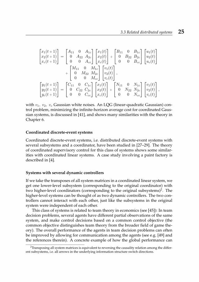
3.3 Related distributed systems 25
x1(t + 1)x2(t + 1)xc(t + 1)
=
A11 0 A1c
0 A22 A2c
0 0 Acc
x1(t)x2(t)xc(t)
+
B11 0 B1c
0 B22 B2c
0 0 Bcc
u1(t)u2(t)uc(t)
+
M11 0 M1c
0 M22 M2c
0 0 Mcc
v1(t)v2(t)vc(t)
,y1(t + 1)y2(t + 1)yc(t + 1)
=
C11 0 C1c
0 C22 C2c
0 0 Ccc
x1(t)x2(t)xc(t)
+
N11 0 N1c
0 N22 N2c
0 0 Ncc
v1(t)v2(t)vc(t)
,with v1, v2, vc Gaussian white noises. An LQG (linear-quadratic Gaussian) con-trol problem, minimizing the infinite-horizon average cost for coordinated Gaus-sian systems, is discussed in [41], and shows many similarities with the theory inChapter 6.
Coordinated discrete-event systems
Coordinated discrete-event systems, i.e. distributed discrete-event systems withseveral subsystems and a coordinator, have been studied in [27–29]. The theoryof coordinated supervisory control for this class of systems shows some similar-ities with coordinated linear systems. A case study involving a paint factory isdescribed in [4].
Systems with several dynamic controllers
If we take the transposes of all system matrices in a coordinated linear system, weget one lower-level subsystem (corresponding to the original coordinator) withtwo higher-level coordinators (corresponding to the original subsystems)2. Thehigher-level systems can be thought of as two dynamic controllers. The two con-trollers cannot interact with each other, just like the subsystems in the originalsystem were independent of each other.
This class of systems is related to team theory in economics (see [45]): In teamdecision problems, several agents have different partial observations of the samesystem, and make control decisions based on a common control objective (thecommon objective distinguishes team theory from the broader field of game the-ory). The overall performance of the agents in team decision problems can oftenbe improved by allowing for communication among the agents (see e.g. [49] andthe references therein). A concrete example of how the global performance can
2Transposing all system matrices is equivalent to reversing the causality relation among the differ-ent subsystems, i.e. all arrows in the underlying information structure switch directions.
26 Chapter 3: Coordinated Linear Systems
be improved by including communication among the controllers on a nearest-neighbor basis is discussed in [39], where different local voltage controllers jointlytry to keep the voltage in a large-scale power network within the safety limits.
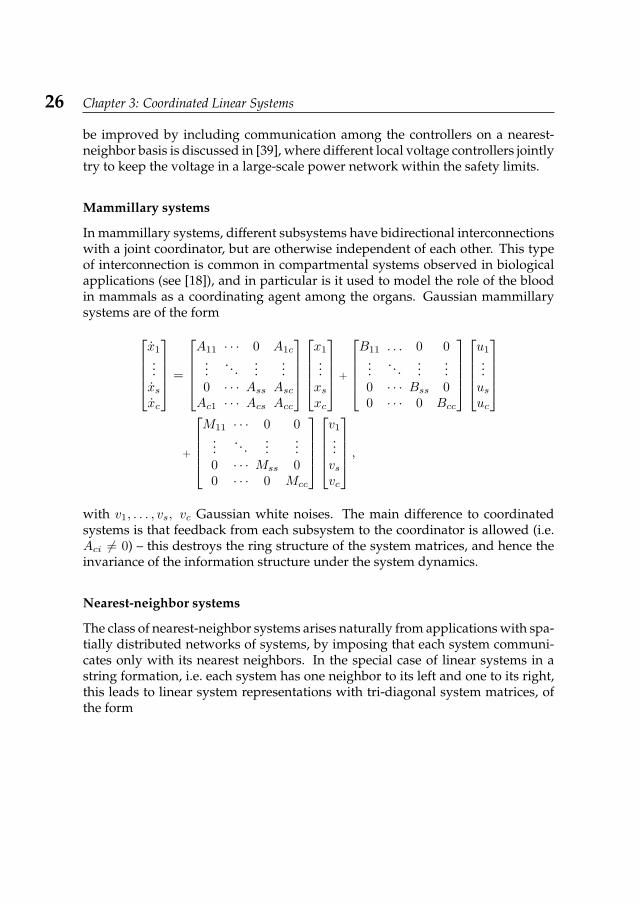
Mammillary systems
In mammillary systems, different subsystems have bidirectional interconnectionswith a joint coordinator, but are otherwise independent of each other. This typeof interconnection is common in compartmental systems observed in biologicalapplications (see [18]), and in particular is it used to model the role of the bloodin mammals as a coordinating agent among the organs. Gaussian mammillarysystems are of the form
x1
...xsxc
=
A11 · · · 0 A1c
.... . .
......
0 · · · Ass AscAc1 · · · Acs Acc
x1
...xsxc
+
B11 . . . 0 0
.... . .
......
0 · · · Bss 00 · · · 0 Bcc
u1
...usuc
+
M11 · · · 0 0
.... . .
......
0 · · · Mss 00 · · · 0 Mcc
v1
...vsvc
,with v1, . . . , vs, vc Gaussian white noises. The main difference to coordinatedsystems is that feedback from each subsystem to the coordinator is allowed (i.e.Aci 6= 0) – this destroys the ring structure of the system matrices, and hence theinvariance of the information structure under the system dynamics.
Nearest-neighbor systems
The class of nearest-neighbor systems arises naturally from applications with spa-tially distributed networks of systems, by imposing that each system communi-cates only with its nearest neighbors. In the special case of linear systems in astring formation, i.e. each system has one neighbor to its left and one to its right,this leads to linear system representations with tri-diagonal system matrices, ofthe form
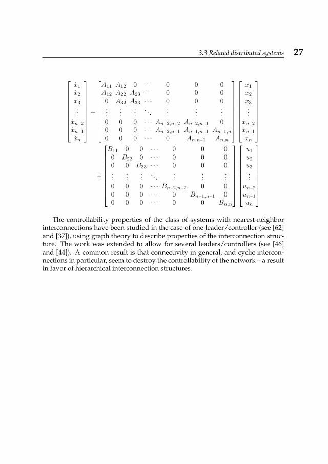
3.3 Related distributed systems 27
x1
x2
x3
...xn−2
xn−1
xn
=
A11 A12 0 · · · 0 0 0A12 A22 A23 · · · 0 0 00 A32 A33 · · · 0 0 0...
......
. . ....
......
0 0 0 · · · An−2,n−2 An−2,n−1 00 0 0 · · · An−2,n−1 An−1,n−1 An−1,n
0 0 0 · · · 0 An,n−1 An,n
x1
x2
x3
...xn−2
xn−1
xn
+
B11 0 0 · · · 0 0 00 B22 0 · · · 0 0 00 0 B33 · · · 0 0 0...
......
. . ....
......
0 0 0 · · · Bn−2,n−2 0 00 0 0 · · · 0 Bn−1,n−1 00 0 0 · · · 0 0 Bn,n
u1
u2
u3
...un−2
un−1
un
The controllability properties of the class of systems with nearest-neighbor
interconnections have been studied in the case of one leader/controller (see [62]and [37]), using graph theory to describe properties of the interconnection struc-ture. The work was extended to allow for several leaders/controllers (see [46]and [44]). A common result is that connectivity in general, and cyclic intercon-nections in particular, seem to destroy the controllability of the network – a resultin favor of hierarchical interconnection structures.
28 Chapter 3: Coordinated Linear Systems
Construction and Minimality 4This chapter deals with the construction and minimality of coordinated linearsystems. Construction procedures are given to transform unstructured or inter-connected systems into coordinated linear systems. Several concepts of minimal-ity for coordinated linear systems are suggested and characterized. A few resultsof this chapter were published in [23].
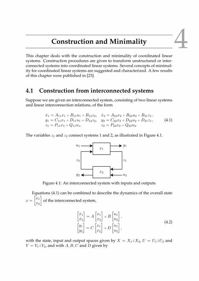
4.1 Construction from interconnected systemsSuppose we are given an interconnected system, consisting of two linear systemsand linear interconnection relations, of the form
x1 = A11x1 + B11u1 + B12z2, x2 = A22x2 + B22u2 + B21z1,y1 = C11x1 + D11u1 + D12z2, y2 = C22x2 + D22u2 + D21z1,z1 = P11x1 + Q11u1, z2 = P22x2 + Q22u2.
(4.1)
The variables z1 and z2 connect systems 1 and 2, as illustrated in Figure 4.1.
x2
x1
u2
y1u1
y2
z1z2
Figure 4.1: An interconnected system with inputs and outputs
Equations (4.1) can be combined to describe the dynamics of the overall state
x =
[x1
x2
]of the interconnected system,
[x1
x2
]= A
[x1
x2
]+ B
[u1
u2
],[
y1
y2
]= C
[x1
x2
]+ D
[u1
u2
],
(4.2)
with the state, input and output spaces given by X = X1+X2, U = U1+U2 andY = Y1+Y2, and with A,B,C and D given by
30 Chapter 4: Construction and Minimality
A =
[A11 B12P22
B21P11 A22
], B =
[B11 B12Q22
B21Q11 B22
],
C =
[C11 D12P22
D21P11 C22
], D =
[D11 D12Q22
D21Q11 D22
].
(4.3)
The problem we consider in this section is how to transform an interconnectedsystem of the form (4.2) into a coordinated linear system. In order to achievethis, the part of system 1 which influences system 2 via z1 will have to be in thecoordinator, and the same holds for system 2.
In other words, we want to decompose the state, input and output space ofthe interconnected system into three parts each, forming a coordinated linear sys-tem. The new subsystem spaces will be denoted by Xi\c, Ui\c, Yi\c, i = 1, 2, thesubscript i\c indicating that part of the original system has been moved to thecoordinator. The new decomposition should respect the original one, in the sensethat the original system 1 will be part of the new subsystem 1\c and the coordi-nator, but not of subsystem 2\c, and vice versa.
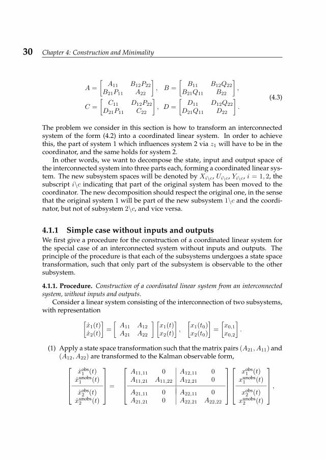
4.1.1 Simple case without inputs and outputsWe first give a procedure for the construction of a coordinated linear system forthe special case of an interconnected system without inputs and outputs. Theprinciple of the procedure is that each of the subsystems undergoes a state spacetransformation, such that only part of the subsystem is observable to the othersubsystem.
4.1.1. Procedure. Construction of a coordinated linear system from an interconnectedsystem, without inputs and outputs.
Consider a linear system consisting of the interconnection of two subsystems,with representation[
x1(t)x2(t)
]=
[A11 A12
A21 A22
] [x1(t)x2(t)
],
[x1(t0)x2(t0)
]=
[x0,1
x0,2
].
(1) Apply a state space transformation such that the matrix pairs (A21, A11) and(A12, A22) are transformed to the Kalman observable form,
xobs1 (t)
xunobs1 (t)
xobs2 (t)
xunobs2 (t)
=
A11,11 0 A12,11 0A11,21 A11,22 A12,21 0
A21,11 0 A22,11 0A21,21 0 A22,21 A22,22
xobs1 (t)
xunobs1 (t)
xobs2 (t)
xunobs2 (t)
,
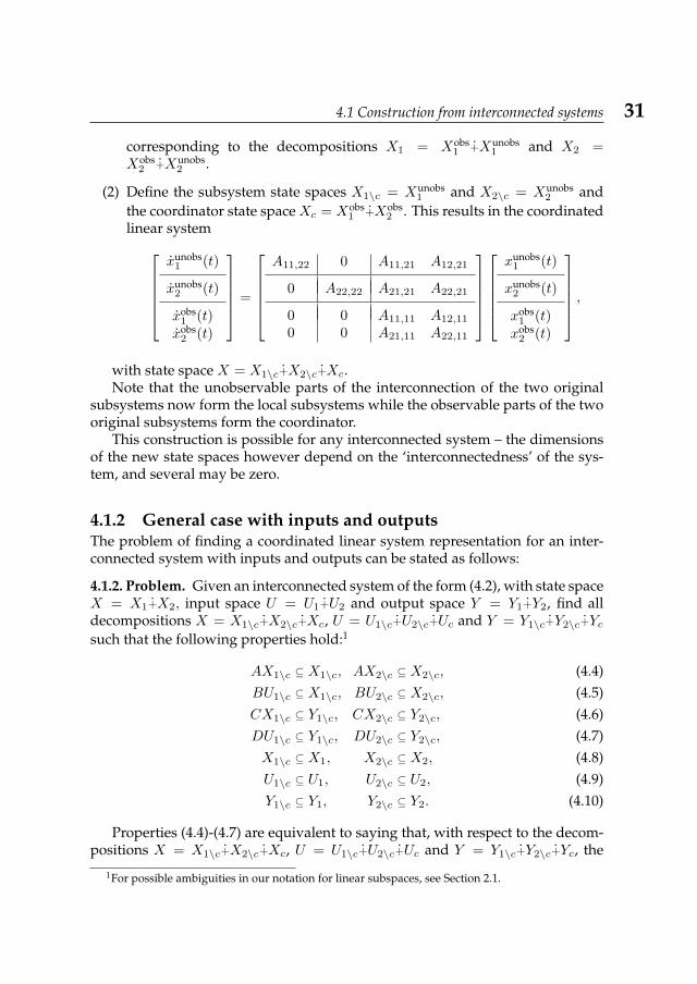
4.1 Construction from interconnected systems 31
corresponding to the decompositions X1 = Xobs1 +Xunobs
1 and X2 =Xobs
2 +Xunobs2 .
(2) Define the subsystem state spaces X1\c = Xunobs1 and X2\c = Xunobs
2 andthe coordinator state space Xc = Xobs
1 +Xobs2 . This results in the coordinated
linear systemxunobs
1 (t)
xunobs2 (t)
xobs1 (t)xobs
2 (t)
=
A11,22 0 A11,21 A12,21
0 A22,22 A21,21 A22,21
0 0 A11,11 A12,11
0 0 A21,11 A22,11
xunobs
1 (t)
xunobs2 (t)
xobs1 (t)xobs
2 (t)
,
with state space X = X1\c+X2\c+Xc.Note that the unobservable parts of the interconnection of the two original
subsystems now form the local subsystems while the observable parts of the twooriginal subsystems form the coordinator.
This construction is possible for any interconnected system – the dimensionsof the new state spaces however depend on the ‘interconnectedness’ of the sys-tem, and several may be zero.
4.1.2 General case with inputs and outputsThe problem of finding a coordinated linear system representation for an inter-connected system with inputs and outputs can be stated as follows:
4.1.2. Problem. Given an interconnected system of the form (4.2), with state spaceX = X1+X2, input space U = U1+U2 and output space Y = Y1+Y2, find alldecompositions X = X1\c+X2\c+Xc, U = U1\c+U2\c+Uc and Y = Y1\c+Y2\c+Ycsuch that the following properties hold:1
AX1\c ⊆ X1\c, AX2\c ⊆ X2\c, (4.4)BU1\c ⊆ X1\c, BU2\c ⊆ X2\c, (4.5)CX1\c ⊆ Y1\c, CX2\c ⊆ Y2\c, (4.6)DU1\c ⊆ Y1\c, DU2\c ⊆ Y2\c, (4.7)X1\c ⊆ X1, X2\c ⊆ X2, (4.8)U1\c ⊆ U1, U2\c ⊆ U2, (4.9)Y1\c ⊆ Y1, Y2\c ⊆ Y2. (4.10)
Properties (4.4)-(4.7) are equivalent to saying that, with respect to the decom-positions X = X1\c+X2\c+Xc, U = U1\c+U2\c+Uc and Y = Y1\c+Y2\c+Yc, the
1For possible ambiguities in our notation for linear subspaces, see Section 2.1.
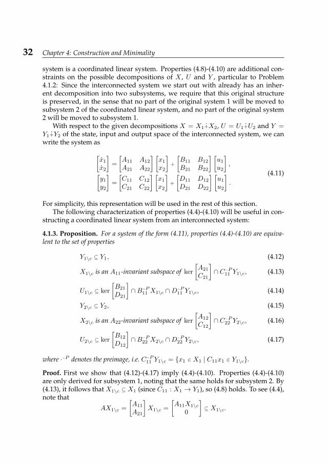
32 Chapter 4: Construction and Minimality
system is a coordinated linear system. Properties (4.8)-(4.10) are additional con-straints on the possible decompositions of X , U and Y , particular to Problem4.1.2: Since the interconnected system we start out with already has an inher-ent decomposition into two subsystems, we require that this original structureis preserved, in the sense that no part of the original system 1 will be moved tosubsystem 2 of the coordinated linear system, and no part of the original system2 will be moved to subsystem 1.
With respect to the given decompositions X = X1+X2, U = U1+U2 and Y =Y1+Y2 of the state, input and output space of the interconnected system, we canwrite the system as[
x1
x2
]=
[A11 A12
A21 A22
] [x1
x2
]+
[B11 B12
B21 B22
] [u1
u2
],[
y1
y2
]=
[C11 C12
C21 C22
] [x1
x2
]+
[D11 D12
D21 D22
] [u1
u2
].
(4.11)
For simplicity, this representation will be used in the rest of this section.The following characterization of properties (4.4)-(4.10) will be useful in con-
structing a coordinated linear system from an interconnected system:
4.1.3. Proposition. For a system of the form (4.11), properties (4.4)-(4.10) are equiva-lent to the set of properties
Y1\c ⊆ Y1, (4.12)
X1\c is an A11-invariant subspace of ker
[A21
C21
]∩ C−P11 Y1\c, (4.13)
U1\c ⊆ ker
[B21
D21
]∩B−P11 X1\c ∩D−P11 Y1\c, (4.14)
Y2\c ⊆ Y2, (4.15)
X2\c is an A22-invariant subspace of ker
[A12
C12
]∩ C−P22 Y2\c, (4.16)
U2\c ⊆ ker
[B12
D12
]∩B−P22 X2\c ∩D−P22 Y2\c, (4.17)
where ·−P denotes the preimage, i.e. C−P11 Y1\c = x1 ∈ X1 | C11x1 ∈ Y1\c.
Proof. First we show that (4.12)-(4.17) imply (4.4)-(4.10). Properties (4.4)-(4.10)are only derived for subsystem 1, noting that the same holds for subsystem 2. By(4.13), it follows that X1\c ⊆ X1 (since C11 : X1 → Y1), so (4.8) holds. To see (4.4),note that
AX1\c =
[A11
A21
]X1\c =
[A11X1\c
0
]⊆ X1\c.
4.1 Construction from interconnected systems 33
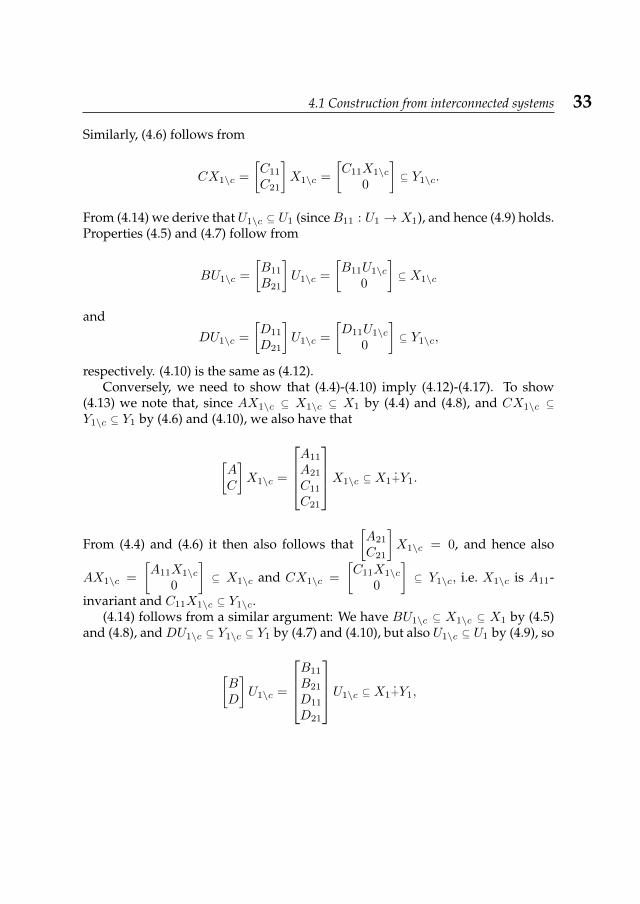
Similarly, (4.6) follows from
CX1\c =
[C11
C21
]X1\c =
[C11X1\c
0
]⊆ Y1\c.
From (4.14) we derive that U1\c ⊆ U1 (sinceB11 : U1 → X1), and hence (4.9) holds.Properties (4.5) and (4.7) follow from
BU1\c =
[B11
B21
]U1\c =
[B11U1\c
0
]⊆ X1\c
and
DU1\c =
[D11
D21
]U1\c =
[D11U1\c
0
]⊆ Y1\c,
respectively. (4.10) is the same as (4.12).Conversely, we need to show that (4.4)-(4.10) imply (4.12)-(4.17). To show
(4.13) we note that, since AX1\c ⊆ X1\c ⊆ X1 by (4.4) and (4.8), and CX1\c ⊆Y1\c ⊆ Y1 by (4.6) and (4.10), we also have that
[AC
]X1\c =
A11
A21
C11
C21
X1\c ⊆ X1+Y1.
From (4.4) and (4.6) it then also follows that[A21
C21
]X1\c = 0, and hence also
AX1\c =
[A11X1\c
0
]⊆ X1\c and CX1\c =
[C11X1\c
0
]⊆ Y1\c, i.e. X1\c is A11-
invariant and C11X1\c ⊆ Y1\c.(4.14) follows from a similar argument: We have BU1\c ⊆ X1\c ⊆ X1 by (4.5)
and (4.8), and DU1\c ⊆ Y1\c ⊆ Y1 by (4.7) and (4.10), but also U1\c ⊆ U1 by (4.9), so
[BD
]U1\c =
B11
B21
D11
D21
U1\c ⊆ X1+Y1,
34 Chapter 4: Construction and Minimality
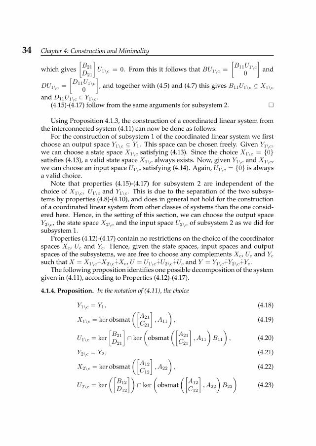
which gives[B21
D21
]U1\c = 0. From this it follows that BU1\c =
[B11U1\c
0
]and
DU1\c =
[D11U1\c
0
], and together with (4.5) and (4.7) this gives B11U1\c ⊆ X1\c
and D11U1\c ⊆ Y1\c.(4.15)-(4.17) follow from the same arguments for subsystem 2.
Using Proposition 4.1.3, the construction of a coordinated linear system fromthe interconnected system (4.11) can now be done as follows:
For the construction of subsystem 1 of the coordinated linear system we firstchoose an output space Y1\c ⊆ Y1. This space can be chosen freely. Given Y1\c,we can choose a state space X1\c satisfying (4.13). Since the choice X1\c = 0satisfies (4.13), a valid state space X1\c always exists. Now, given Y1\c and X1\c,we can choose an input space U1\c satisfying (4.14). Again, U1\c = 0 is alwaysa valid choice.
Note that properties (4.15)-(4.17) for subsystem 2 are independent of thechoice of X1\c, U1\c and Y1\c. This is due to the separation of the two subsys-tems by properties (4.8)-(4.10), and does in general not hold for the constructionof a coordinated linear system from other classes of systems than the one consid-ered here. Hence, in the setting of this section, we can choose the output spaceY2\c, the state space X2\c and the input space U2\c of subsystem 2 as we did forsubsystem 1.
Properties (4.12)-(4.17) contain no restrictions on the choice of the coordinatorspaces Xc, Uc and Yc. Hence, given the state spaces, input spaces and outputspaces of the subsystems, we are free to choose any complements Xc, Uc and Ycsuch that X = X1\c+X2\c+Xc, U = U1\c+U2\c+Uc and Y = Y1\c+Y2\c+Yc.
The following proposition identifies one possible decomposition of the systemgiven in (4.11), according to Properties (4.12)-(4.17).
4.1.4. Proposition. In the notation of (4.11), the choice
Y1\c = Y1, (4.18)
X1\c = ker obsmat([A21
C21
], A11
), (4.19)
U1\c = ker
[B21
D21
]∩ ker
(obsmat
([A21
C21
], A11
)B11
), (4.20)
Y2\c = Y2, (4.21)
X2\c = ker obsmat([A12
C12
], A22
), (4.22)
U2\c = ker
([B12
D12
])∩ ker
(obsmat
([A12
C12
], A22
)B22
)(4.23)
4.1 Construction from interconnected systems 35
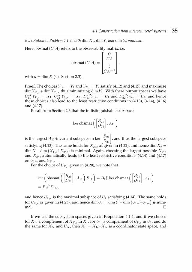
is a solution to Problem 4.1.2, with dimXc, dimYc and dimUc minimal.
Here, obsmat (C,A) refers to the observability matrix, i.e.
obsmat (C,A) =
CCA
...CAn−1
,with n = dimX (see Section 2.3).
Proof. The choices Y1\c = Y1 and Y2\c = Y2 satisfy (4.12) and (4.15) and maximizedimY1\c + dimY2\c, thus minimizing dimYc. With these output spaces we haveC−P11 Y1\c = X1, C−P22 Y2\c = X2, D−P11 Y1\c = U1 and D−P22 Y2\c = U2, and hencethese choices also lead to the least restrictive conditions in (4.13), (4.14), (4.16)and (4.17).
Recall from Section 2.3 that the indistinguishable subspace
ker obsmat([B21
D21
], A11
)
is the largest A11-invariant subspace in ker
[B21
D21
], and thus the largest subspace
satisfying (4.13). The same holds for X2\c as given in (4.22), and hence dimXc =
dimX − dim(X1\c+X2\c
)is minimal. Again, choosing the largest possible X1\c
and X2\c automatically leads to the least restrictive conditions (4.14) and (4.17)on U1\c and U2\c.
For the choice of U1\c given in (4.20), we note that
ker
(obsmat
([B21
D21
], A11
)B11
)= B−P11 ker obsmat
([B21
D21
], A11
)= B−P11 X1\c,
and hence U1\c is the maximal subspace of U1 satisfying (4.14). The same holdsfor U2\c as given in (4.23), and hence dimUc = dimU − dim
(U1\c+U2\c
)is mini-
mal.
If we use the subsystem spaces given in Proposition 4.1.4, and if we choosefor X1c a complement of X1\c in X1, for U1c a complement of U1\c in U1, and dothe same for X2c and U2c, then Xc = X1c+X2c is a coordinator state space, and
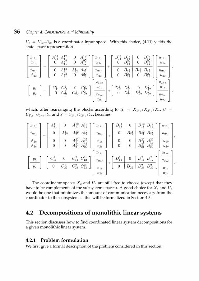
36 Chapter 4: Construction and Minimality
Uc = U1c+U2c is a coordinator input space. With this choice, (4.11) yields thestate-space representationx1\cx1c
x2\cx2c
=
A11
11 A1211 0 A12
12
0 A2211 0 A22
12
0 A1221 A11
22 A1222
0 A2221 0 A22
22
x1\cx1c
x2\cx2c
+
B11
11 B1211 0 B12
12
0 B2211 0 B22
12
0 B1221 B11
22 B1222
0 B2221 0 B22
22
u1\cu1c
u2\cu2c
,[y1
y2
]=
[C1
11 C211 0 C2
12
0 C221 C1
22 C222
]x1\cx1c
x2\cx2c
+
[D1
11 D211 0 D2
12
0 D221 D1
22 D222
]u1\cu1c
u2\cu2c
,which, after rearranging the blocks according to X = X1\c+X2\c+Xc, U =U1\c+U2\c+Uc and Y = Y1\c+Y2\c+Yc, becomes
x1\c
x2\c
x1c
x2c
=
A11
11 0 A1211 A12
12
0 A1122 A12
21 A1222
0 0 A2211 A22
12
0 0 A2221 A22
22
x1\c
x2\c
x1c
x2c
+
B11
11 0 B1211 B12
12
0 B1122 B12
21 B1222
0 0 B2211 B22
12
0 0 B2221 B22
22
u1\c
u2\c
u1c
u2c
,
[y1
y2
]=
[C1
11 0 C211 C2
12
0 C122 C2
21 C222
]x1\c
x2\c
x1c
x2c
+
[D1
11 0 D211 D2
12
0 D122 D2
21 D222
]u1\c
u2\c
u1c
u2c
.
The coordinator spaces Xc and Uc are still free to choose (except that theyhave to be complements of the subsystem spaces). A good choice for Xc and Ucwould be one that minimizes the amount of communication necessary from thecoordinator to the subsystems – this will be formalized in Section 4.3.
4.2 Decompositions of monolithic linear systemsThis section discusses how to find coordinated linear system decompositions fora given monolithic linear system.
4.2.1 Problem formulationWe first give a formal description of the problem considered in this section:
4.2 Decompositions of monolithic linear systems 37
4.2.1. Problem. Consider the monolithic linear system
x = Ax + Bu,
y = Cx,(4.24)
with state space X = Rn, input space U = Rm, output space Y = Rp and initialstate x0 ∈ X . Find the number s ∈ N of subsystems, and decompositions
X = X1\c+ . . . +Xs\c+Xc,
U = U1\c + . . . +Us\c +Uc ,
Y = Y1\c + . . . +Ys\c +Yc ,
such that for all j = 1, . . . , s:
AXj\c ⊆ Xj\c, BUj\c ⊆ Xj\c and CXj\c ⊆ Yj\c.2 (4.25)
When dealing with linear systems, one usually assumes that B has full col-umn rank and C has full row rank. This assumption is natural for monolithiclinear systems:
• If B is not of full column rank then the input space U can be reduced with-out changing the controllability properties of the system.
• If C is not of full row rank then the output space Y can be reduced withoutchanging the observability properties of the system.
For decentralized systems, these assumptions are not useful: For example, thestate of a subsystem may be controllable both via its local input or via the co-ordinator input, so if we were to restrict attention to the usual concept of con-trollability then one of these inputs is irrelevant to the system. However, for localcontrollability it is important that the subsystem is controllable via the local input,and for coordinator controllability it is important that the subsystem is control-lable via the coordinator input (these concepts will be defined and discussed inChapter 5). Even though both inputs can control the same part of the state, theirdifferent locations in the decentralized system distinguish them, and (in general)neither of them should be removed from the system.
Similarly, different outputs in a decentralized system may have different rolesin the system even though they both observe the same part of the state: If a sub-system output and a coordinator output both observe the same part of the coordi-nator state, then this state information is available both locally and remotely, andhence both the coordinator itself and the subsystem observing this part can use
2Note that such a decomposition always exists: The (trivial) decomposition X = Xc, Y = Yc,U = Uc satisfies these conditions.
38 Chapter 4: Construction and Minimality
this information for control purposes, without the coordinator having to commu-nicate its observations.
The difference between Problem 4.2.1 and Problem 4.1.2 from the previous sectionis that no a priori decomposition of the original system into two parts is given,i.e. conditions (4.8)-(4.10) are dropped from the problem. These conditions sepa-rated the overall decomposition problem into two independent subproblems (i.e.each original subsystem has to be separated into a local part and a coordinatorpart). Dropping these conditions means that we have more freedom in choosingour decompositions, but also that we lose the independence property of the dif-ferent subproblems. In fact, part of Problem 4.2.1 is to first identify the differentsubproblems – this also means that choosing the number of subsystems s is partof the problem.
Our approach in the following is to first decompose the state spaceX into sev-eral subsystems according to the invariance properties of A, and then applying aresult similar to Proposition 4.1.3.
4.2.2 Systems without inputs and outputsThe first problem we need to consider is how to split the monolithic system intodifferent subsystems, and how many subsystems to expect. An important prop-erty of subsystems is that their state spaces should be A-invariant – this suggeststhat we consider the Jordan normal form of A (see [40]):
There exists a decomposition3
X = X1+X2+ . . . +Xs,
and let the transformed system be given byx1
x2
...xs
=
J1 0 · · · 00 J2 · · · 0...
.... . .
...0 0 · · · Js
x1
x2
...xs
,where the Jj are the different Jordan blocks. We notice that the Jordan normalform of A naturally splits the system into s independent subsystems, one foreach Jordan block. This decomposition is ‘as decentralized as possible’, i.e. split-ting any Jordan block into two subsystems will destroy the A-invariance of thesubsystem. Hence, to summarize, by taking the Jordan decomposition, we have
3If A is assumed to be non-derogatory then the number of different A-invariant spaces in X isfinite. In that case, the Jordan decomposition of X is unique up to reordering.
4.2 Decompositions of monolithic linear systems 39
found the number of subsystems s and the state spaces of the different subsys-tems, and any further decomposition would lose the A-invariance property.
For systems without inputs and outputs, this is the most straightforward wayof splitting up a monolithic system into subsystems. Since we consider systemswith inputs and outputs, the condition AXj ⊆ Xj is not the only one the statespace has to satisfy, and hence a further decomposition of the state space will benecessary.
4.2.3 Systems with inputs and outputsWe first rewrite conditions (4.25) into a more constructive form, similar to condi-tions (4.12)-(4.17) for interconnected systems:
4.2.2. Proposition. With i ∈ 1, . . . , s, there exist linearly independent subspacesXi\c ⊆ X , Ui\c ⊆ U and Yi\c ⊆ Y , such that (4.25) holds, if and only if there existKi, Kc, Li, Lc, Xi\c, Xc, Ui\c, Uc, Yi\c and Yc such that
Y = Y1\c+ . . . +Ys\c+Yc, (4.26)kerC = K1+ . . . +Ks+Kc, (4.27)kerB = L1+ . . . +Ls+Lc, (4.28)
For j = 1, . . . , s, Xj\c is an A-invariant subspace of C−PYj\c with Xj\c ∩ kerC ⊆ Kj ,(4.29)
Xc is a complement of X1\c+ . . . +Xs\c in X, (4.30)
For j = 1, . . . , s, Uj\c is a subspace of B−PXj\c with Uj\c ∩ kerB ⊆ Lj , (4.31)Uc is a complement of U1\c+ . . . +Us\c in U . (4.32)
Proof. Conditions (4.26)-(4.32) indeed lead to decompositions of X , U and Y : Forj 6= k ∈ 1, . . . , swe have
Xj\c ∩Xk\c ⊆ C−P(Yj\c ∩ Yk\c
)= C−P 0 = kerC,
but Xj\c ∩ kerC ⊆ Kj and hence Xj\c ∩Xk\c ⊆ Kj ∩Kk = 0. Similarly,
Uj\c ∩ Uk\c ⊆ B−P(Xj\c ∩Xk\c
)= B−P 0 = kerB,
but Uj\c ∩ kerB ⊆ Lj and hence Uj\c ∩ Uk\c ⊆ Lj ∩ Lk = 0. For Y we have adecomposition given in (4.26). In addition, (4.25) is clearly satisfied, by (4.29) and(4.31).
Conversely, let decompositions of X , Y and U be given such that (4.25) holds.Then (4.26), (4.30) and (4.32) are automatically satisfied. Observe that for i 6= jwe have
(Xi\c ∩ kerC) ∩ (Xj\c ∩ kerC) = 0.
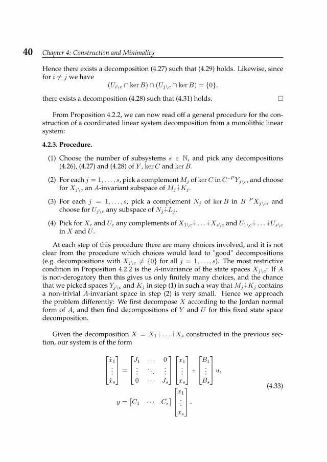
40 Chapter 4: Construction and Minimality
Hence there exists a decomposition (4.27) such that (4.29) holds. Likewise, sincefor i 6= j we have
(Ui\c ∩ kerB) ∩ (Uj\c ∩ kerB) = 0,
there exists a decomposition (4.28) such that (4.31) holds.
From Proposition 4.2.2, we can now read off a general procedure for the con-struction of a coordinated linear system decomposition from a monolithic linearsystem:
4.2.3. Procedure.
(1) Choose the number of subsystems s ∈ N, and pick any decompositions(4.26), (4.27) and (4.28) of Y , kerC and kerB.
(2) For each j = 1, . . . , s, pick a complementMj of kerC inC−PYj\c, and choosefor Xj\c an A-invariant subspace of Mj+Kj .
(3) For each j = 1, . . . , s, pick a complement Nj of kerB in B−PXj\c, andchoose for Uj\c any subspace of Nj+Lj .
(4) Pick for Xc and Uc any complements of X1\c+ . . . +Xs\c and U1\c+ . . . +Us\cin X and U .
At each step of this procedure there are many choices involved, and it is notclear from the procedure which choices would lead to "good" decompositions(e.g. decompositions with Xj\c 6= 0 for all j = 1, . . . , s). The most restrictivecondition in Proposition 4.2.2 is the A-invariance of the state spaces Xj\c: If Ais non-derogatory then this gives us only finitely many choices, and the chancethat we picked spaces Yj\c and Kj in step (1) in such a way that Mj+Kj containsa non-trivial A-invariant space in step (2) is very small. Hence we approachthe problem differently: We first decompose X according to the Jordan normalform of A, and then find decompositions of Y and U for this fixed state spacedecomposition.
Given the decomposition X = X1+ . . . +Xs constructed in the previous sec-tion, our system is of the formx1
...xs
=
J1 · · · 0...
. . ....
0 · · · Js
x1
...xs
+
B1
...Bs
u,
y =[C1 · · · Cs
] x1
...xs
.(4.33)
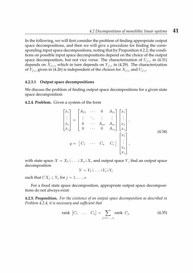
4.2 Decompositions of monolithic linear systems 41
In the following, we will first consider the problem of finding appropriate outputspace decompositions, and then we will give a procedure for finding the corre-sponding input space decompositions, noting that by Proposition 4.2.2, the condi-tions on possible input space decompositions depend on the choice of the outputspace decomposition, but not vice versa: The characterization of Uj\c in (4.31)depends on Xj\c, which in turn depends on Yj\c in (4.29). The characterizationof Yj\c given in (4.26) is independent of the choices for Xj\c and Uj\c.
4.2.3.1 Output space decompositions
We discuss the problem of finding output space decompositions for a given statespace decomposition:
4.2.4. Problem. Given a system of the formx1
...xsxc
=
A11 · · · 0 A1c
.... . .
......
0 · · · Ass Asc0 · · · 0 Acc
x1
...xsxc
,
y =[C1 · · · Cs Cc
]x1
...xsxc
,(4.34)
with state space X = X1+ . . . +Xs+Xc and output space Y , find an output spacedecomposition
Y = Y1+ . . . +Ys+Yc
such that CXj ⊆ Yj for j = 1, . . . , s.
For a fixed state space decomposition, appropriate output space decomposi-tions do not always exist:
4.2.5. Proposition. For the existence of an output space decomposition as described inProblem 4.2.4, it is necessary and sufficient that
rank[C1 . . . Cs
]=
∑j=1,...,s
rank Cj . (4.35)
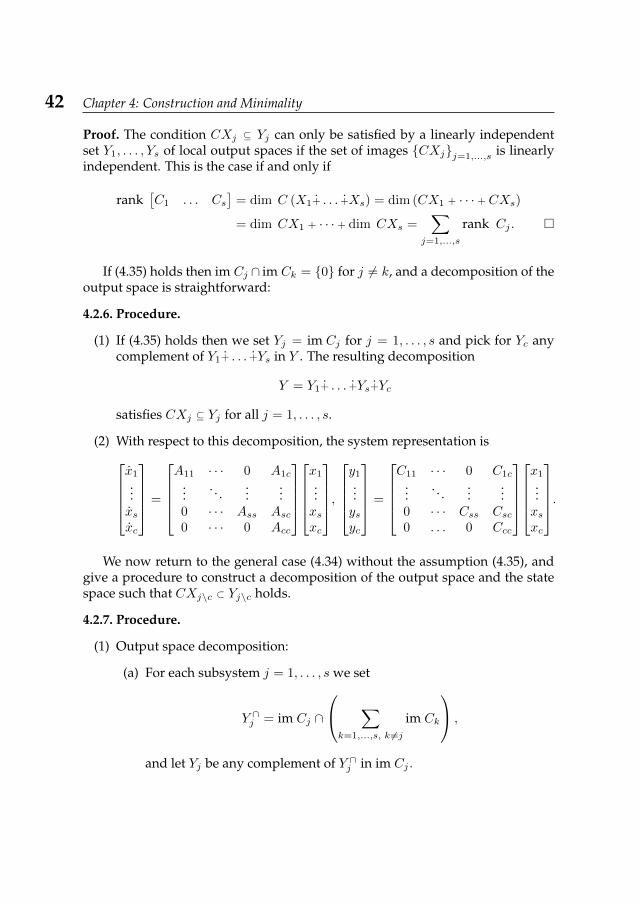
42 Chapter 4: Construction and Minimality
Proof. The condition CXj ⊆ Yj can only be satisfied by a linearly independentset Y1, . . . , Ys of local output spaces if the set of images CXjj=1,...,s is linearlyindependent. This is the case if and only if
rank[C1 . . . Cs
]= dim C (X1+ . . . +Xs) = dim (CX1 + · · · + CXs)
= dim CX1 + · · · + dim CXs =∑
j=1,...,s
rank Cj .
If (4.35) holds then im Cj ∩ im Ck = 0 for j 6= k, and a decomposition of theoutput space is straightforward:
4.2.6. Procedure.
(1) If (4.35) holds then we set Yj = im Cj for j = 1, . . . , s and pick for Yc anycomplement of Y1+ . . . +Ys in Y . The resulting decomposition
Y = Y1+ . . . +Ys+Yc
satisfies CXj ⊆ Yj for all j = 1, . . . , s.
(2) With respect to this decomposition, the system representation isx1
...xsxc
=
A11 · · · 0 A1c
.... . .
......
0 · · · Ass Asc0 · · · 0 Acc
x1
...xsxc
,y1
...ysyc
=
C11 · · · 0 C1c
.... . .
......
0 · · · Css Csc0 . . . 0 Ccc
x1
...xsxc
.
We now return to the general case (4.34) without the assumption (4.35), andgive a procedure to construct a decomposition of the output space and the statespace such that CXj\c ⊂ Yj\c holds.
4.2.7. Procedure.
(1) Output space decomposition:
(a) For each subsystem j = 1, . . . , s we set
Y ∩j = im Cj ∩
∑k=1,...,s, k 6=j
im Ck
,
and let Yj be any complement of Y ∩j in im Cj .
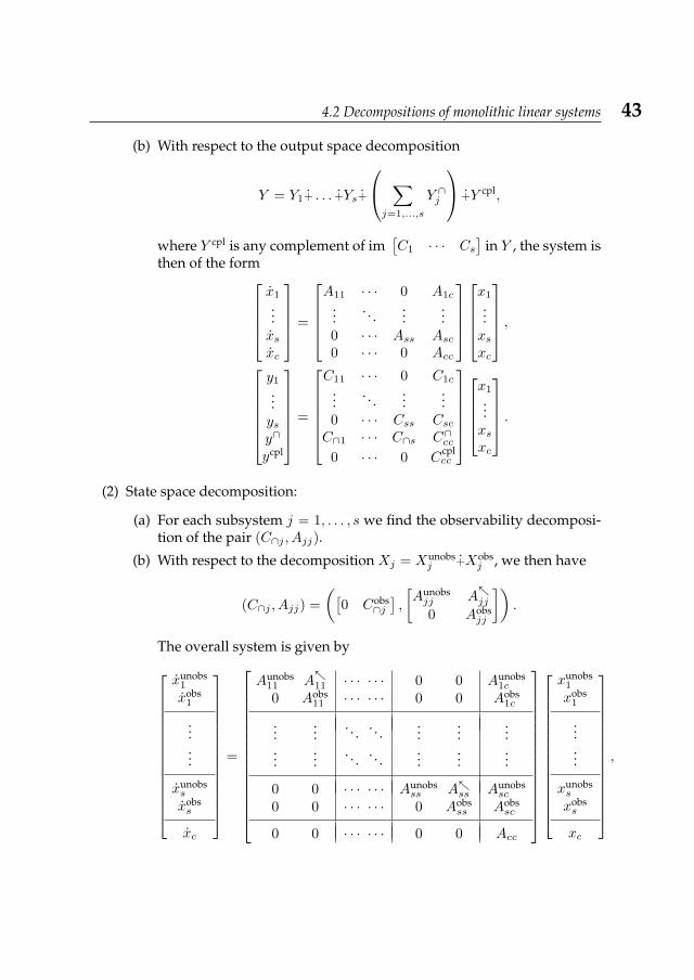
4.2 Decompositions of monolithic linear systems 43
(b) With respect to the output space decomposition
Y = Y1+ . . . +Ys+
∑j=1,...,s
Y ∩j
+Y cpl,
where Y cpl is any complement of im[C1 · · · Cs
]in Y , the system is
then of the formx1
...xsxc
=
A11 · · · 0 A1c
.... . .
......
0 · · · Ass Asc0 · · · 0 Acc
x1
...xsxc
,y1
...ysy∩
ycpl
=
C11 · · · 0 C1c
.... . .
......
0 · · · Css CscC∩1 · · · C∩s C∩cc
0 · · · 0 Ccplcc
x1
...xsxc
.
(2) State space decomposition:
(a) For each subsystem j = 1, . . . , s we find the observability decomposi-tion of the pair (C∩j , Ajj).
(b) With respect to the decomposition Xj = Xunobsj +Xobs
j , we then have
(C∩j , Ajj) =
([0 Cobs
∩j],
[Aunobsjj Ajj0 Aobs
jj
]).
The overall system is given by
xunobs1
xobs1
...
...
xunobss
xobss
xc
=
Aunobs11 A11 · · · · · · 0 0 Aunobs
1c
0 Aobs11 · · · · · · 0 0 Aobs
1c
......
. . . . . ....
......
......
. . . . . ....
......
0 0 · · · · · · Aunobsss Ass Aunobs
sc
0 0 · · · · · · 0 Aobsss Aobs
sc
0 0 · · · · · · 0 0 Acc
xunobs1
xobs1
...
...
xunobss
xobss
xc
,
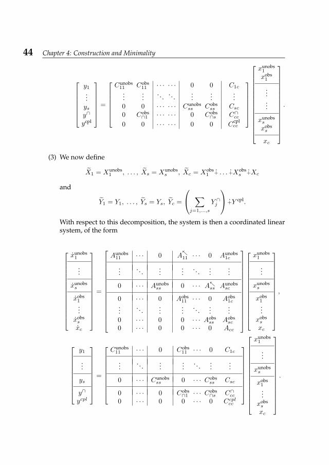
44 Chapter 4: Construction and Minimality
y1
...ysy∩
ycpl
=
Cunobs
11 Cobs11 · · · · · · 0 0 C1c
......
. . . . . ....
......
0 0 · · · · · · Cunobsss Cobs
ss Csc0 Cobs
∩1 · · · · · · 0 Cobs∩s C∩cc
0 0 · · · · · · 0 0 Ccplcc
xunobs1
xobs1
...
...
xunobss
xobss
xc
.
(3) We now define
X1 = Xunobs1 , . . . , Xs = Xunobs
s , Xc = Xobs1 + . . . +Xobs
s +Xc
and
Y1 = Y1, . . . , Ys = Ys, Yc =
∑j=1,...,s
Y ∩j
+Y cpl.
With respect to this decomposition, the system is then a coordinated linearsystem, of the form
xunobs1
...
xunobss
xobs1...
xobss
xc
=
Aunobs11 · · · 0 A11 · · · 0 Aunobs
1c
.... . .
......
. . ....
...
0 · · · Aunobsss 0 · · · Ass Aunobs
sc
0 · · · 0 Aobs11 · · · 0 Aobs
1c...
. . ....
.... . .
......
0 · · · 0 0 · · · Aobsss Aobs
sc
0 · · · 0 0 · · · 0 Acc
xunobs1
...
xunobss
xobs1...
xobss
xc
,
y1
...
ys
y∩
ycpl
=
Cunobs11 · · · 0 Cobs
11 · · · 0 C1c
.... . .
......
. . ....
...
0 · · · Cunobsss 0 · · · Cobs
ss Csc
0 · · · 0 Cobs∩1 · · · Cobs
∩s C∩cc0 · · · 0 0 · · · 0 Ccplcc
xunobs1
...
xunobss
xobs1...
xobss
xc
.

4.2 Decompositions of monolithic linear systems 45
This procedure does not necessarily lead to a decomposition with a minimalcoordinator state space: Moving Xobs
1 + . . . +Xobss to the coordinator state space is
sufficient for satisfying (4.35), but may not be necessary.
4.2.3.2 Input space decompositions
The problem of finding appropriate input space decompositions for a given statespace decomposition will be discussed next:
4.2.8. Problem. Given a system of the formx1
...xsxc
=
A11 · · · 0 A1c
.... . .
......
0 · · · Ass Asc0 · · · 0 Acc
x1
...xsxc
+
B1
...BsBc
u,with state space X = X1+ . . . +Xs+Xc and input space U , find an input spacedecomposition
U = U1+ . . . +Us+Uc
such that BUj ⊆ Xj for j = 1, . . . , s.4
This problem is straightforwardly solved by applying the following proce-dure:
4.2.9. Procedure.
(1) Pick an arbitrary decomposition
kerB = Uker1 + . . . +Uker
s +Ukerc
of kerB.
(2) For each subsystem j = 1, . . . , s, let U cplj be any complement of kerB in the
space ⋂k=1,...,s,c, k 6=j
kerBk.
(3) Now we set the subsystem input spaces to Uj = Ukerj +U
cplj . With Uc any
complement of U1+ . . . +Us in U , we now have
U = U1+ . . . +Us+Uc,
and BUj = BUkerj + BU
cplj = BU
cplj = BjU
cplj ⊆ Xj .
4Such an input space decomposition always exists: Take U = Uc.
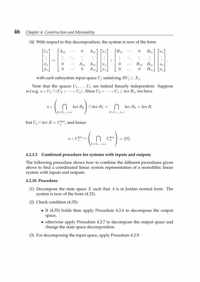
46 Chapter 4: Construction and Minimality
(4) With respect to this decomposition, the system is now of the formx1
...xsxc
=
A11 · · · 0 A1c
.... . .
......
0 · · · Ass Asc0 · · · 0 Acc
x1
...xsxc
+
B11 · · · 0 B1c
.... . .
......
0 · · · Bss Bsc0 . . . 0 Bcc
u1
...usuc
,with each subsystem input space Uj satisfying BUj ⊆ Xj .
Note that the spaces U1, . . . , Us are indeed linearly independent: Supposew.l.o.g. u ∈ U1 ∩ (U2 + · · · + Us) . Since U2 + · · · + Us ⊆ kerB1, we have
u ∈
⋂k=2,...,s,c
kerBk
∩ kerB1 =⋂
k=1,...,s,c
kerBk = kerB,
but Uj ∩ kerB = Ukerj , and hence
u ∈ Uker1 ∩
⋂k=2,...,s,c
Ukerk
= 0.
4.2.3.3 Combined procedure for systems with inputs and outputs
The following procedure shows how to combine the different procedures givenabove to find a coordinated linear system representation of a monolithic linearsystem with inputs and outputs:
4.2.10. Procedure.
(1) Decompose the state space X such that A is in Jordan normal form. Thesystem is now of the form (4.33).
(2) Check condition (4.35):
• If (4.35) holds then apply Procedure 4.2.6 to decompose the outputspace,
• otherwise apply Procedure 4.2.7 to decompose the output space andchange the state space decomposition.
(3) For decomposing the input space, apply Procedure 4.2.9.
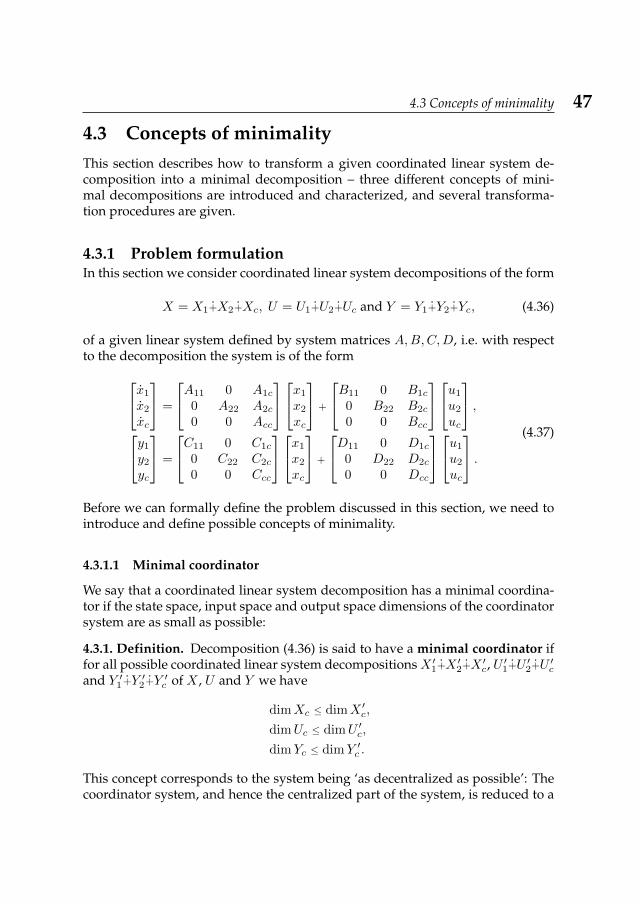
4.3 Concepts of minimality 47
4.3 Concepts of minimalityThis section describes how to transform a given coordinated linear system de-composition into a minimal decomposition – three different concepts of mini-mal decompositions are introduced and characterized, and several transforma-tion procedures are given.
4.3.1 Problem formulationIn this section we consider coordinated linear system decompositions of the form
X = X1+X2+Xc, U = U1+U2+Uc and Y = Y1+Y2+Yc, (4.36)
of a given linear system defined by system matrices A,B,C,D, i.e. with respectto the decomposition the system is of the formx1
x2
xc
=
A11 0 A1c
0 A22 A2c
0 0 Acc
x1
x2
xc
+
B11 0 B1c
0 B22 B2c
0 0 Bcc
u1
u2
uc
,y1
y2
yc
=
C11 0 C1c
0 C22 C2c
0 0 Ccc
x1
x2
xc
+
D11 0 D1c
0 D22 D2c
0 0 Dcc
u1
u2
uc
.(4.37)
Before we can formally define the problem discussed in this section, we need tointroduce and define possible concepts of minimality.
4.3.1.1 Minimal coordinator
We say that a coordinated linear system decomposition has a minimal coordina-tor if the state space, input space and output space dimensions of the coordinatorsystem are as small as possible:
4.3.1. Definition. Decomposition (4.36) is said to have a minimal coordinator iffor all possible coordinated linear system decompositionsX ′1+X ′2+X ′c, U ′1+U ′2+U ′cand Y ′1 +Y ′2 +Y ′c of X , U and Y we have
dimXc ≤ dimX ′c,
dimUc ≤ dimU ′c,
dimYc ≤ dimY ′c .
This concept corresponds to the system being ‘as decentralized as possible’: Thecoordinator system, and hence the centralized part of the system, is reduced to a
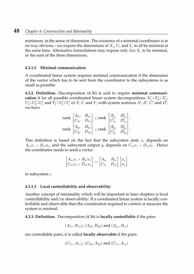
48 Chapter 4: Construction and Minimality
minimum, in the sense of dimension. The existence of a minimal coordinator is inno way obvious – we require the dimensions of Xc, Uc and Yc to all be minimal atthe same time. Alternative formulations may require only dimXc to be minimal,or the sum of the three dimensions.
4.3.1.2 Minimal communication
A coordinated linear system requires minimal communication if the dimensionof the vector which has to be sent from the coordinator to the subsystems is assmall as possible:
4.3.2. Definition. Decomposition (4.36) is said to require minimal communi-cation if for all possible coordinated linear system decompositions X ′1+X ′2+X ′c,U ′1+U ′2+U ′c and Y ′1 +Y ′2 +Y ′c of X , U and Y , with system matrices A′, B′, C ′ and D′,we have
rank[A1c B1c
C1c D1c
]≤ rank
[A′1c B′1cC ′1c D′1c
],
rank[A2c B2c
C2c D2c
]≤ rank
[A′2c B′2cC ′2c D′2c
].
This definition is based on the fact that the subsystem state xi depends onAicxc + Bicuc, and the subsystem output yi depends on Cicxc + Dicuc. Hencethe coordinator needs to send a vector[
Aicxc + BicucCicxc + Dicuc
]=
[Aic BicCic Dic
] [xcuc
]to subsystem i.
4.3.1.3 Local controllability and observability
Another concept of minimality which will be important in later chapters is localcontrollability and/or observability: If a coordinated linear system is locally con-trollable and observable then the coordination required to control or measure thesystem is minimal.
4.3.3. Definition. Decomposition (4.36) is locally controllable if the pairs
(A11, B11), (A22, B22) and (Acc, Bcc)
are controllable pairs; it is called locally observable if the pairs
(C11, A11), (C22, A22) and (Ccc, Acc)
4.3 Concepts of minimality 49
are observable pairs.
This definition is a short version of the definitions and characterizations in Sec-tions 5.2.3.2 and 5.3.3.2, where these concepts are described in more detail.
4.3.1.4 Problem formulation
Given the concepts of minimality defined above, we can now formulate the prob-lems considered in this section:
4.3.4. Problem. Given a coordinated linear system of the form (4.37), with re-spect to a decomposition of the form (4.36), and given the concepts of minimalitydefined in Definitions 4.3.1, 4.3.2 and 4.3.3,
• under which conditions do minimal decompositions exist,
• and how can the given decomposition be transformed into a minimal de-composition?
Some considerations and partial results concerning this problem are given inthe following subsections.
4.3.2 Minimality of the coordinatorFor interconnected systems, we have already found a decomposition with a min-imal coordinator in Proposition 4.1.4. However, this was based on the extra con-dition that the original decompositions X = X1+X2, U = U1+U2 and Y = Y1+Y2
are respected.For the more general case of decomposing monolithic linear systems, we
found that a construction procedure similar to the one given for interconnectedsystems is not useful in practice, and Procedure 4.2.10 generally does not lead toa minimal coordinator. In particular, if condition (4.35) is not satisfied then Pro-cedure 4.2.7 has to be applied, which leads to an unnecessarily large coordinatorstate space. Moreover, reducing the number of subsystems s may lead to smallercoordinator spaces – in fact, if s = 1, i.e. there is only one subsystem, then nocoordination is required at all.
In the following we assume that the decompositions (4.36) are already fixed,and we describe how to reduce the coordinator spaces, noting again that the statespace decomposition depends on the output space decomposition but not viceversa, and the input space decomposition depends on the state space and outputspace decompositions but not vice versa.
The minimal coordinator output space is always Yc = 0: We can alwaysmove the coordinator output space to a (new or existing) subsystem without vio-lating the underlying information structure. This would however lead to a locallyunobservable system, as discussed in Section 4.3.4.
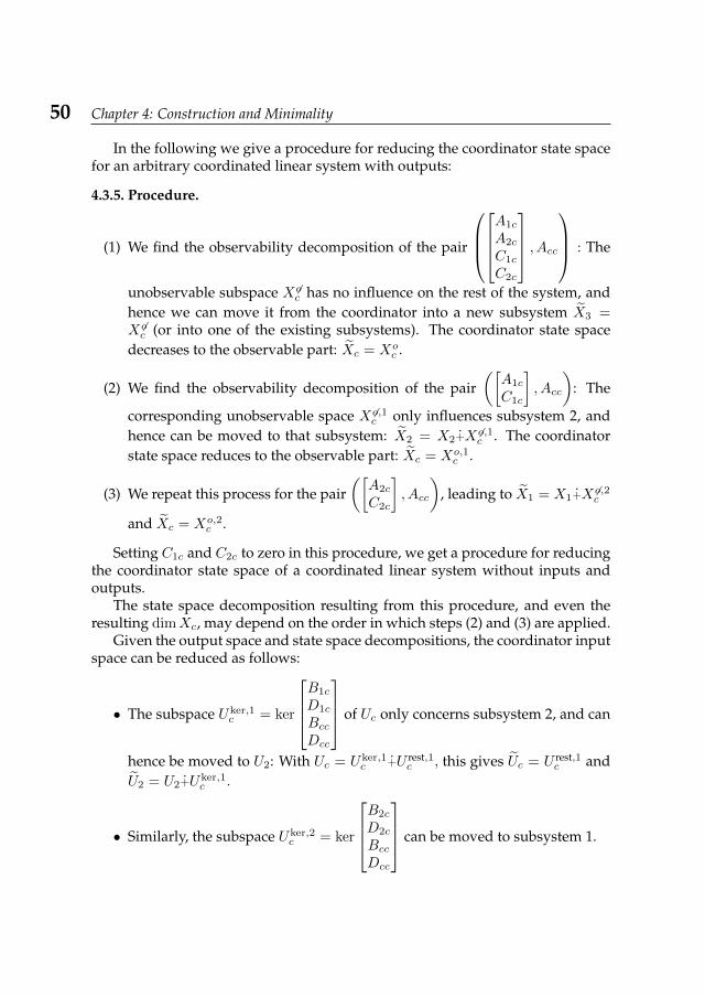
50 Chapter 4: Construction and Minimality
In the following we give a procedure for reducing the coordinator state spacefor an arbitrary coordinated linear system with outputs:
4.3.5. Procedure.
(1) We find the observability decomposition of the pair
A1c
A2c
C1c
C2c
, Acc : The
unobservable subspace X 6oc has no influence on the rest of the system, andhence we can move it from the coordinator into a new subsystem X3 =X 6oc (or into one of the existing subsystems). The coordinator state spacedecreases to the observable part: Xc = Xo
c .
(2) We find the observability decomposition of the pair([A1c
C1c
], Acc
): The
corresponding unobservable space X 6o,1c only influences subsystem 2, andhence can be moved to that subsystem: X2 = X2+X 6o,1c . The coordinatorstate space reduces to the observable part: Xc = Xo,1
c .
(3) We repeat this process for the pair([A2c
C2c
], Acc
), leading to X1 = X1+X 6o,2c
and Xc = Xo,2c .
Setting C1c and C2c to zero in this procedure, we get a procedure for reducingthe coordinator state space of a coordinated linear system without inputs andoutputs.
The state space decomposition resulting from this procedure, and even theresulting dimXc, may depend on the order in which steps (2) and (3) are applied.
Given the output space and state space decompositions, the coordinator inputspace can be reduced as follows:
• The subspace Uker,1c = ker
B1c
D1c
BccDcc
of Uc only concerns subsystem 2, and can
hence be moved to U2: With Uc = Uker,1c +U rest,1
c , this gives Uc = U rest,1c and
U2 = U2+Uker,1c .
• Similarly, the subspace Uker,2c = ker
B2c
D2c
BccDcc
can be moved to subsystem 1.
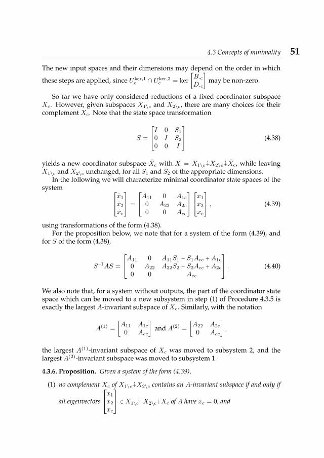
4.3 Concepts of minimality 51
The new input spaces and their dimensions may depend on the order in which
these steps are applied, since Uker,1c ∩ Uker,2
c = ker
[B·cD·c
]may be non-zero.
So far we have only considered reductions of a fixed coordinator subspaceXc. However, given subspaces X1\c and X2\c, there are many choices for theircomplement Xc. Note that the state space transformation
S =
I 0 S1
0 I S2
0 0 I
(4.38)
yields a new coordinator subspace Xc with X = X1\c+X2\c+Xc, while leavingX1\c and X2\c unchanged, for all S1 and S2 of the appropriate dimensions.
In the following we will characterize minimal coordinator state spaces of thesystem x1
x2
xc
=
A11 0 A1c
0 A22 A2c
0 0 Acc
x1
x2
xc
, (4.39)
using transformations of the form (4.38).For the proposition below, we note that for a system of the form (4.39), and
for S of the form (4.38),
S−1AS =
A11 0 A11S1 − S1Acc + A1c
0 A22 A22S2 − S2Acc + A2c
0 0 Acc
. (4.40)
We also note that, for a system without outputs, the part of the coordinator statespace which can be moved to a new subsystem in step (1) of Procedure 4.3.5 isexactly the largest A-invariant subspace of Xc. Similarly, with the notation
A(1) =
[A11 A1c
0 Acc
]and A(2) =
[A22 A2c
0 Acc
],
the largest A(1)-invariant subspace of Xc was moved to subsystem 2, and thelargest A(2)-invariant subspace was moved to subsystem 1.
4.3.6. Proposition. Given a system of the form (4.39),
(1) no complement Xc of X1\c+X2\c contains an A-invariant subspace if and only if
all eigenvectors
x1
x2
xc
∈ X1\c+X2\c+Xc of A have xc = 0, and
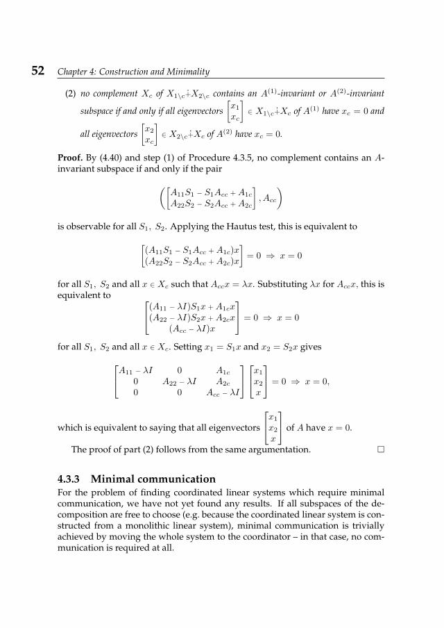
52 Chapter 4: Construction and Minimality
(2) no complement Xc of X1\c+X2\c contains an A(1)-invariant or A(2)-invariant
subspace if and only if all eigenvectors[x1
xc
]∈ X1\c+Xc of A(1) have xc = 0 and
all eigenvectors[x2
xc
]∈ X2\c+Xc of A(2) have xc = 0.
Proof. By (4.40) and step (1) of Procedure 4.3.5, no complement contains an A-invariant subspace if and only if the pair([
A11S1 − S1Acc + A1c
A22S2 − S2Acc + A2c
], Acc
)is observable for all S1, S2. Applying the Hautus test, this is equivalent to[
(A11S1 − S1Acc + A1c)x(A22S2 − S2Acc + A2c)x
]= 0 ⇒ x = 0
for all S1, S2 and all x ∈ Xc such that Accx = λx. Substituting λx for Accx, this isequivalent to (A11 − λI)S1x + A1cx
(A22 − λI)S2x + A2cx(Acc − λI)x
= 0 ⇒ x = 0
for all S1, S2 and all x ∈ Xc. Setting x1 = S1x and x2 = S2x givesA11 − λI 0 A1c
0 A22 − λI A2c
0 0 Acc − λI
x1
x2
x
= 0 ⇒ x = 0,
which is equivalent to saying that all eigenvectors
x1
x2
x
of A have x = 0.
The proof of part (2) follows from the same argumentation.
4.3.3 Minimal communicationFor the problem of finding coordinated linear systems which require minimalcommunication, we have not yet found any results. If all subspaces of the de-composition are free to choose (e.g. because the coordinated linear system is con-structed from a monolithic linear system), minimal communication is triviallyachieved by moving the whole system to the coordinator – in that case, no com-munication is required at all.
4.3 Concepts of minimality 53
If we assume that the state, input and output spaces of the subsystems arefixed, and in line with the previous subsection, we can reduce the problem to find-ing complementsXc ofX1\c+X2\c inX , Uc of U1\c+U2\c in U , and Yc of Y1\c+Y2\cin Y , such that the resulting decomposition requires minimal communication:
Define the transformations
R =
I 0 R1c
0 I R2c
0 0 I
: Y → Y, S =
I 0 S1c
0 I S2c
0 0 I
: X → X,
and T =
I 0 T1c
0 I T2c
0 0 I
: U → U,
where the submatrices Ric, Sic and Tic are free to choose. The problem we wantto solve can then be written as
minR,S,T
rank[
(SAS−1)1c (SBT −1)1c
(RCS−1)1c (RDT −1)1c
], (4.41)
minR,S,T
rank[
(SAS−1)2c (SBT −1)2c
(RCS−1)2c (RDT −1)2c
]. (4.42)
For A,B,C,D given in (4.37), we have[(SAS−1)1c (SBT −1)1c
(RCS−1)1c (RDT −1)1c
]=
[A1c −A11S1c + S1cAcc B1c −B11T1c + S1cBccC1c − C11S1c + R1cCcc D1c −D11T1c + R1cDcc
],[
(SAS−1)2c (SBT −1)2c
(RCS−1)2c (RDT −1)2c
]=
[A2c −A22S2c + S2cAcc B2c −B22T2c + S2cBccC2c − C22S2c + R2cCcc D2c −D22T2c + R2cDcc
].
From this we can see that the two subproblems decouple – in (4.41) weneed to minimize over R1c, S1c, T1c and (4.42) is a minimization problem overR2c, S2c, T2c.
For the special case of a system without inputs and outputs, the minimizationproblem given in (4.41) reduces to
minS1c:Xc→X1
rank (A1c −A11S1c + S1cAcc) . (4.43)
The solution to this problem follows directly from [47, Theorem 2.1], a simplifiedversion of which is quoted for convenience:
54 Chapter 4: Construction and Minimality
Define s(A1, A2) = maxλ∈C min dim ker (A1 − λI) ,dim ker (A2 − λI) .Consider the linear Sylvester map T : Cp×q → Cp×q defined by
T (S) = SA2 −A1S, S ∈ Cp×q,
(a) Every matrix X ∈ Cp×q can be written in the form
X = T (S) + Y,
for some S ∈ Cp×q and Y ∈ Cp×q with rank Y ≤ s(A1, A2).
(b) Assume that s(A1, A2) 6= 0. Then for fixed A1 and A2 thereis a Zariski open nonempty set Ω of Cp×q such that for everyX ∈ Ω there is no representation of X in the form
X = T (S) + Y,
where S, Y ∈ Cp×q are such that rank Y < s(A1, A2).
Translated to the minimization problem in (4.43), this means that
minS1c:Xc→X1
rank (A1c −A11S1c + S1cAcc) ≤ s(A11, Acc),
and that this upper bound is attained for all A1c in a Zariski open nonemptysubset of Cn1×nc (i.e. for "almost all" A1c).
4.3.4 Local observability and controllabilityThe following result concerns the existence of locally controllable or observabledecompositions:
4.3.7. Proposition. For the existence of a locally controllable coordinated linear systemdecomposition it is necessary and sufficient that the pair (A,B) is a controllable pair.The existence of a local observable decomposition is equivalent to the pair (C,A) being anobservable pair.
Proof. By the block-triangular structure of A and B, local controllability is astronger concept than controllability of (A,B). Conversely, if (A,B) is a con-trollable pair then setting Xc = X and Uc = U trivially leads to a locallycontrollable system. The same argument holds for local observability, using theblock-triangular structure of C and A.
For coordinated linear systems with inputs, a state space transformationwhich renders the system locally controllable is straightforward:
4.3 Concepts of minimality 55
4.3.8. Procedure. We assume that the pair (A,B) is a controllable pair.
(1) For each subsystem i = 1, 2 we find the controllability decomposition of(Aii, Bii), i.e. we decompose the subsystem state space into Xi = Xc
i +X 6ccsuch that with respect to this decomposition we have
(Aii, Bii) =
([Acii Aii0 A 6cii
],
[Bcii0
]),
with (Acii, Bcii) a controllable pair.
(2) We reduce the subsystem state spaces to their controllable parts and movethe uncontrollable parts to the coordinator, i.e. we reset
X1 := Xc1 , X2 := Xc
2 , and Xc := X 6c1+X 6c2+Xc.
(3) With respect to the new state space decomposition, the system representa-tion becomesxc1xc2
x 6c1x 6c2xc
=
Ac11 0 A11 0 Ac1c0 Ac22 0 A22 Ac2c
0 0 A 6c11 0 A 6c1c0 0 0 A 6c22 A 6c2c0 0 0 0 Acc
xc1xc2
x 6c1x 6c2xc
+
Bc11 0 Bc1c0 Bc22 Bc2c
0 0 B 6c1c0 0 B 6c2c0 0 Bcc
u1
u2
uc
.
Now the subsystems are locally controllable by construction. Suppose there isa locally uncontrollable mode in the coordinator, then this mode is uncontrollablein the usual sense (since the only option for controlling the coordinator state is viathe coordinator input), but the system is controllable in the usual sense, whichcontradicts the assumption. Hence the system resulting from this procedure islocally controllable.
Note that in Procedure 4.3.8 we only applied a state space transformation,but left the input spaces unchanged. In some situations it might be useful tomove parts of the coordinator input to a subsystem in order to achieve localcontrollability, instead of moving parts of the subsystem state to the coordinator.However, if we start out with a decomposition in which the coordinator inputspace has minimal dimension then the procedure above leads to a locally con-trollable system with minimal coordinator state and input spaces.
For the transformation of a coordinated linear system into a locally observableform, and in line with the previous section, we find that there are different choicesto consider:
4.3.9. Procedure. We assume that pair (C,A) is an observable pair.
56 Chapter 4: Construction and Minimality
(1) We find the observability decomposition of the coordinator pair (Ccc, Acc),i.e. we decompose the coordinator state space into Xc = X 6oc +Xo
c , such that
(Ccc, Acc) =
([0 Cocc
],
[A 6occ Acc0 Aocc
]),
with (Cocc, Aocc) an observable pair.
(2) If X 6oc is[A1c
C1c
]-unobservable then X 6oc can move to subsystem 2. Similarly, it
may move to subsystem 1 if it is[A2c
C2c
]-unobservable.
(3) Otherwise, pick decompositions Y1 = Y 6m1 +Y m1 and Y2 = Y 6m2 +Y m2 of thesubsystem output spaces, such that X 6oc is observable from Y m1 +Y m2 .
(4) We reset the output spaces,
Y1 := Y 6m1 , Y2 := Y 6m2 , Yc := Yc+Ym1 +Y m2 ,
and the state spaces,
X1 is any A-invariant subspace of C−PY1,
X2 is any A-invariant subspace of C−PY2,
Xc is any complement of X1+X2 in X .
Now the coordinator system is locally observable by construction. Thesubsystems are locally observable since (C,A) was assumed to be observable.Picking the decompositions in step (3) is a difficult problem – in practice, thiscan be done by choosing one output vector at a time and testing whether theunobservable subspace X 6oc would decrease if that vector were in the coordinator.Moreover, the dimensions of the coordinator spaces resulting from this proce-dure depend on which choices are made.
A combined procedure for transforming a coordinated linear system with in-puts and outputs into a locally controllable and observable system would be toiterate Procedures 4.3.8 and 4.3.9: Several iterations may be needed since apply-ing Procedure 4.3.9 to a locally controllable system may render the system locallyuncontrollable, and Procedure 4.3.8 may destroy local observability.
Controllability and Observability 5This chapter deals with the controllability and observability properties of coordi-nated linear systems, and was published as [25].
5.1 IntroductionControl theory is typically concerned with controlling global behavior of a sys-tem. For large systems consisting of several interconnected parts, it is of particu-lar interest whether these global properties can be achieved via local control: Theidea is to solve a control problem of lower complexity for each part of the systemseparately, and ideally these solutions would combine to a control law achievingthe desired global property. The structure of coordinated systems allows for localcontrol synthesis in a top-to-bottom manner, by first finding a control law for thecoordinator, and then controlling each subsystem separately. For this, it is rele-vant which part of the system is controllable by using which input: Subsystem i,with state space Xi, may be controllable via its local input ui, or via the coordina-tor input uc, or both. The coordinator can only be controllable via the coordinatorinput uc.
Moreover, decentralized systems are typically set up in such a way that eachpart of the system only has access to partial information about the system state:Each part of the system can observe (part of) its local state, and possibly the stateof other, usually neighboring, parts of the system. In order to obtain informationabout the global state of the system, it is then necessary for the different parts tocommunicate their observations to each other. This communication, and hencethe availability of global state information, is restricted by the information struc-ture imposed on the system. In particular, the coordinator of a coordinated linearsystem can only observe (part of) its own state. The subsystems, on the otherhand, can observe (part of) their local state and the coordinator state, where thecoordinator state can be observed by subsystem i either indirectly via its influenceon the local state xi, or directly via communication from the coordinator.
In this chapter, we study the controllability and observability properties ofcoordinated linear systems, taking into account the different locations and rolesof the available inputs and outputs, in order to provide a conceptual frameworkfor future research on control synthesis for coordinated linear systems.
The results in this chapter make extensive use of the properties of reachableand indistinguishable subspaces summarized in Section 2.3, and the controlla-bility and observability decompositions derived for coordinated linear systemscombine the corresponding Kalman decompositions with the special structure ofthe system matrices in (3.1).
58 Chapter 5: Controllability and Observability
Note that for linear systems, the concepts of controllability and observabilityare dual to each other: The matrix pair (A,B) is a controllable pair if and onlyif the transposed pair (BT , AT ) is an observable pair. However, for coordinatedlinear systems, this duality cannot be used to reduce one of the two conceptsto the other one: If the matrix pair (A,B) corresponds to a coordinated linearsystem then the transposed pair (BT , AT ) does not represent a coordinated linearsystem, unless A and B are block-diagonal. Hence, the concepts of controllabilityand observability for coordinated linear systems are treated separately in thischapter.
The outline of the chapter is as follows: In Section 5.2, we refine the usualconcept of reachability, taking into account which input is used to reach a state,and which part of the system the reachable state corresponds to. Using theseconcepts, we then derive a controllability decomposition for coordinated linearsystems, and discuss several possibilities for defining the concept of controllabil-ity in this setting. In Section 5.3 the usual concept of indistinguishability is refinedin a similar manner, an observability decomposition for coordinated linear sys-tems is derived, and several possible concepts of observability for this class ofsystems are defined and discussed. The combination of the different conceptsof controllability and observability, for the purpose of stabilization via measure-ment feedback or the characterization of other forms of output controllability, isdiscussed in Section 5.4, and some conclusions are given in Section 5.5.
5.2 ControllabilityIn this section we consider coordinated linear systems with inputs and withoutoutputs, i.e. systems of the form
x(t) =
A11 0 A1c
0 A22 A2c
0 0 Acc
x(t) +
B11 0 B1c
0 B22 B2c
0 0 Bcc
u(t), (5.1)
with x(t) =
x1(t)x2(t)xc(t)
and u(t) =
u1(t)u2(t)uc(t)
.
In the following we will refine the usual concept of reachability, taking intoaccount which input is used to reach a state, and which part of the system thereachable state corresponds to. Using these concepts, we will then derive a con-trollability decomposition for coordinated linear systems, and discuss severalpossibilities for defining the concept of controllability in this setting.
5.2 Controllability 59
5.2.1 ReachabilityFor monolithic linear systems, the concept of reachability describes whether thereexists a piecewise-continuous input trajectory, such that a given state x ∈ X canbe reached from the zero initial state in finite time (see e.g. [21]).
For coordinated linear systems it is not only interesting whether a state can bereached, but also which input is used to reach it: While a subsystem state xi maybe reachable via the local input ui, or the coordinator input uc, or a combinationof the two, a coordinator state xc can only be reached via the coordinator inputuc. This restriction is due to the condition BUi ⊆ Xi in Definition 3.1.1. Forthis reason, the usual definition of reachability is not satisfactory for coordinatedlinear systems. We introduce several concepts which are related to, but differentfrom the definition of reachability as quoted in Section 2.3. In these new concepts,special attention is paid to specifying whether a state is reachable using the localinput or the coordinator input.
5.2.1. Definition. We define the following concepts of reachability:1
• For i = 1, 2, a state xi ∈ Xi is called ui-reachable (i.e. reachable using thelocal input ui) if there exist a finite terminal time t ∈ [0,∞) and a piecewise-continuous input trajectory ui : [0, t]→ Ui such that the system
xi(t) = Aiixi(t) + Biiui(t), xi(0) = 0
has a state trajectory xi : [0, t] → Xi satisfying xi(t) = xi. The set of allui-reachable states xi ∈ Xi will be denoted by Ri.
• A state x ∈ X is called uc-reachable (i.e. reachable using the coordinatorinput uc) if there exist a finite terminal time t ∈ [0,∞) and a piecewise-continuous input trajectory uc : [0, t]→ Uc such that the system
x(t) =
A11 0 A1c
0 A22 A2c
0 0 Acc
x(t) +
B1c
B2c
Bcc
uc(t), x(0) =
000
has a state trajectory x : [0, t] → X satisfying x(t) = x. The set of all uc-reachable states x ∈ X will be denoted by Rc.
Note that R1, R2 and Rc are reachable subspaces of three different linear sys-tems, and hence these subspaces have the following properties (see [72]):
• R1 is the smallest A11-invariant subspace of X1 containing im B11,
• R2 is the smallest A22-invariant subspace of X2 containing im B22,
1Note that we use X1 to denote both the space X1 and the subspace
I00
X1 ⊆ X (see Section 2.1).
60 Chapter 5: Controllability and Observability
• and Rc is the smallest A-invariant subspace of X containing im
B1c
B2c
Bcc
.
Recall from Section 2.3 that the linear subspace R ⊆ X was defined as the setof all reachable states in the usual sense. The concepts of Definition 5.2.1 relate tothe usual concept of reachability as follows:
5.2.2. Lemma. For the set R of all reachable states, the following relation holds:
R =
I00
R1 +
0I0
R2 + Rc. (5.2)
Lemma 5.2.2 implies that our choice of definitions of R1, R2 and Rc complieswith our intuitive conception of reachability: A state is reachable if and only if itcan be reached via a combination of the available control inputs, and this is thecase if and only if it is a combination of several states, each of which is reachablevia one of the control inputs.
Proof. By (2.3) and with the notation C (A,B) =[B AB A2B . . . An−1B
],
we have
R =im C (A,B) = im C
A,B11 0 B1c
0 B22 B2c
0 0 Bcc
=im C
A,B11
00
+ im C
A, 0B22
0
+ im C
A,B1c
B2c
Bcc
=im
B11 A11B11 . . . An−111 B11
0 0 . . . 00 0 . . . 0
+ im
0 0 . . . 0B22 A22B22 . . . An−1
22 B22
0 0 . . . 0
+ im C
A,B1c
B2c
Bcc
=
I00
im C (A11, B11) +
0I0
im C (A22, B22) + im C
A,B1c
B2c
Bcc
=
I00
R1 +
0I0
R2 + Rc.
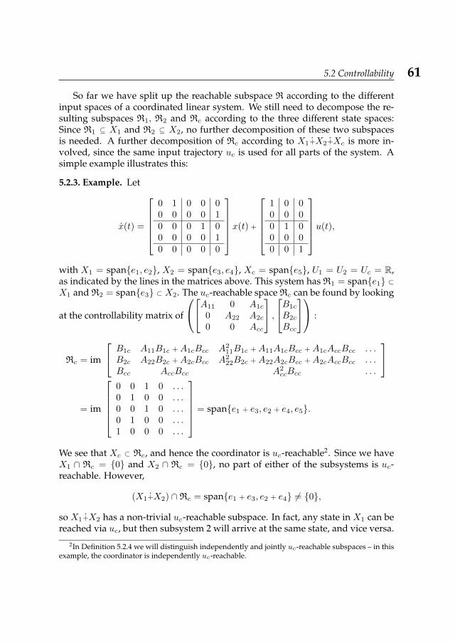
5.2 Controllability 61
So far we have split up the reachable subspace R according to the differentinput spaces of a coordinated linear system. We still need to decompose the re-sulting subspaces R1, R2 and Rc according to the three different state spaces:Since R1 ⊆ X1 and R2 ⊆ X2, no further decomposition of these two subspacesis needed. A further decomposition of Rc according to X1+X2+Xc is more in-volved, since the same input trajectory uc is used for all parts of the system. Asimple example illustrates this:
5.2.3. Example. Let
x(t) =
0 1 0 0 00 0 0 0 10 0 0 1 00 0 0 0 10 0 0 0 0
x(t) +
1 0 00 0 00 1 00 0 00 0 1
u(t),
with X1 = spane1, e2, X2 = spane3, e4, Xc = spane5, U1 = U2 = Uc = R,as indicated by the lines in the matrices above. This system has R1 = spane1 ⊂X1 and R2 = spane3 ⊂ X2. The uc-reachable space Rc can be found by looking
at the controllability matrix of
A11 0 A1c
0 A22 A2c
0 0 Acc
,B1c
B2c
Bcc
:
Rc = im
B1c A11B1c + A1cBcc A211B1c + A11A1cBcc + A1cAccBcc . . .
B2c A22B2c + A2cBcc A222B2c + A22A2cBcc + A2cAccBcc . . .
Bcc AccBcc A2ccBcc . . .
= im
0 0 1 0 . . .0 1 0 0 . . .0 0 1 0 . . .0 1 0 0 . . .1 0 0 0 . . .
= spane1 + e3, e2 + e4, e5.
We see that Xc ⊂ Rc, and hence the coordinator is uc-reachable2. Since we haveX1 ∩ Rc = 0 and X2 ∩ Rc = 0, no part of either of the subsystems is uc-reachable. However,
(X1+X2) ∩Rc = spane1 + e3, e2 + e4 6= 0,
so X1+X2 has a non-trivial uc-reachable subspace. In fact, any state in X1 can bereached via uc, but then subsystem 2 will arrive at the same state, and vice versa.
2In Definition 5.2.4 we will distinguish independently and jointly uc-reachable subspaces – in thisexample, the coordinator is independently uc-reachable.
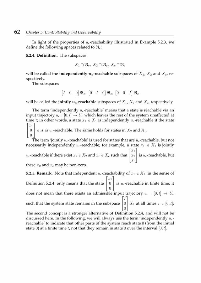
62 Chapter 5: Controllability and Observability
In light of the properties of uc-reachability illustrated in Example 5.2.3, wedefine the following spaces related to Rc:
5.2.4. Definition. The subspaces
X1 ∩Rc, X2 ∩Rc, Xc ∩Rc
will be called the independently uc-reachable subspaces of X1, X2 and Xc, re-spectively.
The subspaces [I 0 0
]Rc,
[0 I 0
]Rc,
[0 0 I
]Rc
will be called the jointly uc-reachable subspaces of X1, X2 and Xc, respectively.
The term ‘independently uc-reachable’ means that a state is reachable via aninput trajectory uc : [0, t] → Uc which leaves the rest of the system unaffected attime t; in other words, a state x1 ∈ X1 is independently uc-reachable if the statex1
00
∈ X is uc-reachable. The same holds for states in X2 and Xc.
The term ‘jointly uc-reachable’ is used for states that are uc-reachable, but notnecessarily independently uc-reachable; for example, a state x1 ∈ X1 is jointly
uc-reachable if there exist x2 ∈ X2 and xc ∈ Xc such that
x1
x2
xc
is uc-reachable, but
these x2 and xc may be non-zero.
5.2.5. Remark. Note that independent uc-reachability of x1 ∈ X1, in the sense of
Definition 5.2.4, only means that the state
x1
00
is uc-reachable in finite time; it
does not mean that there exists an admissible input trajectory uc : [0, t] → Uc
such that the system state remains in the subspace
I00
X1 at all times τ ∈ [0, t]:
The second concept is a stronger alternative of Definition 5.2.4, and will not bediscussed here. In the following, we will always use the term ‘independently uc-reachable’ to indicate that other parts of the system reach state 0 (from the initialstate 0) at a finite time t, not that they remain in state 0 over the interval [0, t].
5.2 Controllability 63
The subspaces of Definition 5.2.4 can be combined to form over- and under-approximations of Rc: It immediately follows from Definition 5.2.4 that
(X1 ∩Rc)+(X2 ∩Rc)+(Xc ∩Rc) ⊆ Rc, (5.3)
Rc ⊆[I 0 0
]Rc+
[0 I 0
]Rc+
[0 0 I
]Rc. (5.4)
Note that the inclusions in (5.3) and (5.4) are in general not equalities.
5.2.2 Controllability decompositionUsing the definitions and results of Section 5.2.1, we will now derive a decompo-sition of the state space X according to the reachable spaces R1, R2 and Rc, andthe underlying decomposition X = X1+X2+Xc.
We start by looking at the state space X1 of subsystem 1: We have that
R1 ⊆ X1 and X1 ∩Rc ⊆[I 0 0
]Rc ⊆ X1, (5.5)
where R1 is the u1-reachable space, X1 ∩ Rc is the independently uc-reachablesubspace of X1, and
[I 0 0
]Rc is the jointly uc-reachable subspace of X1.
We decompose X1 according to the following procedure:
5.2.6. Procedure.
(1) Let X11 = R1 ∩ (X1 ∩Rc), and observe that then X1
1 ⊆ R1 ∩[I 0 0
]Rc.
(2) Take for X21 a complement of X1
1 in R1 ∩[I 0 0
]Rc.
(3) LetX31 be a complement ofX1
1 +X21 in R1. Note that nowX1
1 +X21 +X3
1 = R1.
(4) Likewise, asX11 ⊆ X1∩Rc,we can letX4
1 be a complement ofX11 inX1∩Rc.
Observe that X41 ∩R1 = 0, and R1 + (X1 ∩Rc) = X1
1 +X21 +X3
1 +X41 .
(5) Next, we letX51 be a complement ofX1
1 +X21 +X4
1 in[I 0 0
]Rc, observing
thatX11 +X2
1 +X41 is indeed a subspace of
[I 0 0
]Rc, sinceX4
1 ⊆ X1∩Rc ⊆[I 0 0
]Rc by (5.5).
(6) X61 is a complement of X1
1 +X21 +X3
1 +X41 +X5
1 in X1.
This construction can be done numerically, by first picking a basisB1 forX11 =
R1 ∩ (X1 ∩Rc), and then extending B1 to obtain bases for the other subspaces inthe decomposition.
Now we can write
X1 = X11 +X2
1 +X31 +X4
1 +X51 +X6
1 .
64 Chapter 5: Controllability and Observability
Note that one or more of these subspaces can be 0.The reachability properties of the elements of this decomposition are given in
the following table:
subspace u1-reachable uc-reachableX1
1 yes independentlyX2
1 yes only jointlyX3
1 yes noX4
1 no independentlyX5
1 no only jointlyX6
1 no no
The decomposition of X2 is analogous, with the same reachability properties.For the decomposition of the coordinator state space, we have to take into
account the subspaces Xc ∩Rc ⊆[0 0 I
]Rc ⊆ Xc.
5.2.7. Procedure.
(1) We set X1c = Xc ∩Rc.
(2) We let X2c be a complement of X1
c in[0 0 I
]Rc.
(3) For X3c we choose any complement of X1
c +X2c in Xc.
Now we can writeXc = X1
c +X2c +X3
c .
Now X1c is independently uc-reachable, X2
c is only jointly uc-reachable, and X3c
is not reachable at all.
The following theorem is the main result of this section. It describes the in-variance and controllability properties of the system given in (5.1), using the de-composition derived above.
5.2.8. Theorem. With respect to the state space decomposition
X = (X11 + . . . +X6
1 ) + (X12 + . . . +X6
2 ) + (X1c +X2
c +X3c ) (5.6)
defined by Procedures 5.2.6 and 5.2.7, the system given in (5.1) has the form given inTable 5.1.
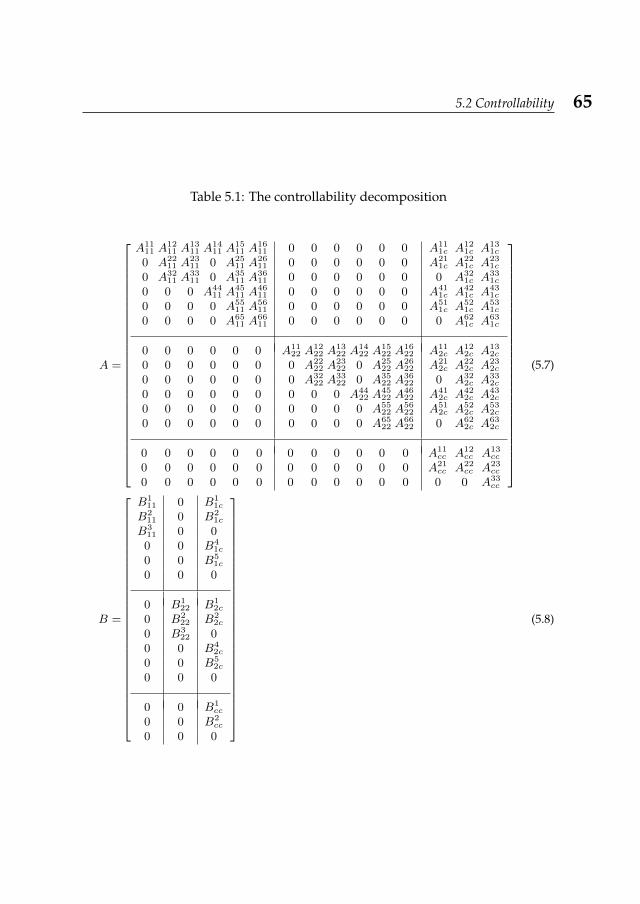
5.2 Controllability 65
Table 5.1: The controllability decomposition
A =
A1111 A12
11 A1311 A14
11 A1511 A16
11 0 0 0 0 0 0 A111c A12
1c A131c
0 A2211 A23
11 0 A2511 A26
11 0 0 0 0 0 0 A211c A22
1c A231c
0 A3211 A33
11 0 A3511 A36
11 0 0 0 0 0 0 0 A321c A33
1c
0 0 0 A4411 A45
11 A4611 0 0 0 0 0 0 A41
1c A421c A43
1c
0 0 0 0 A5511 A56
11 0 0 0 0 0 0 A511c A52
1c A531c
0 0 0 0 A6511 A66
11 0 0 0 0 0 0 0 A621c A63
1c
0 0 0 0 0 0 A1122 A12
22 A1322 A14
22 A1522 A16
22 A112c A12
2c A132c
0 0 0 0 0 0 0 A2222 A23
22 0 A2522 A26
22 A212c A22
2c A232c
0 0 0 0 0 0 0 A3222 A33
22 0 A3522 A36
22 0 A322c A33
2c
0 0 0 0 0 0 0 0 0 A4422 A45
22 A4622 A41
2c A422c A43
2c
0 0 0 0 0 0 0 0 0 0 A5522 A56
22 A512c A52
2c A532c
0 0 0 0 0 0 0 0 0 0 A6522 A66
22 0 A622c A63
2c
0 0 0 0 0 0 0 0 0 0 0 0 A11cc A12
cc A13cc
0 0 0 0 0 0 0 0 0 0 0 0 A21cc A22
cc A23cc
0 0 0 0 0 0 0 0 0 0 0 0 0 0 A33cc
(5.7)
B =
B111 0 B1
1c
B211 0 B2
1c
B311 0 00 0 B4
1c
0 0 B51c
0 0 0
0 B122 B1
2c
0 B222 B2
2c
0 B322 0
0 0 B42c
0 0 B52c
0 0 0
0 0 B1cc
0 0 B2cc
0 0 0
(5.8)
66 Chapter 5: Controllability and Observability
In the notation of Table 5.1, and with i = 1, 2, the following pairs are controllablepairs:
A11ii A12
ii A13ii
0 A22ii A23
ii
0 A32ii A33
ii
,B1
ii
B2ii
B3ii
,
A11
11 A1411 0 0 A1
1c
0 A4411 0 0 A4
1c
0 0 A1122 A14
22 A12c
0 0 0 A4422 A4
2c
0 0 0 0 A11cc
,B1
1c
B41c
B12c
B42c
B1cc
([A11cc A12
cc
A21cc A22
cc
],
[B1cc
B2cc
]).
(5.9)
Proof. Recall from Definitions 3.1.1 and 5.2.1 that the subspaces X1 and Rc areA-invariant. Since R1 ⊆ X1 is A11-invariant, its embedding into X is A-invariant.Now X1
1 = R1 ∩ (X1 ∩ Rc) is an intersection of A-invariant spaces, and henceA-invariant, which gives the first column of A in Table 5.1. The second and thirdcolumn follow from X1
1 +X21 +X3
1 = R1 being A-invariant (as a subspace of X).The A-invariance of X1 ∩Rc = X1
1 +X41 explains the fourth column. The fifth and
sixth column follow from the A-invariance of X1. Similar arguments establishcolumns 7 - 12 for subsystem 2.
For establishing columns 13 and 14 of A, we note that
X1c +X2
c =[0 0 I
]Rc =
[0 0 I
]im C
A,B1c
B2c
Bcc
= im
[Bcc AccBcc A2
ccBcc . . .]
= im C (Acc, Bcc) ,
and hence[0 0 I
]Rc = X1
c +X2c is Acc-invariant. Moreover,
A(Xc ∩Rc) ⊆ Rc ⊆[I 0 0
]Rc+
[0 I 0
]Rc+
[0 0 I
]Rc
= (X11 +X2
1 +X41 +X5
1 )+(X12 +X2
2 +X42 +X5
2 )+(X1c +X2
c ),
which gives that no part of (X31 +X6
1 )+(X32 +X6
2 )+X3c is uc-reachable.
The structure of the B-matrix follows from
im B11 ⊆ R1 = X11 +X2
1 +X31 , im B22 ⊆ R2 = X1
2 +X22 +X3
2 ,
im
B1c
B2c
Bcc
⊆ Rc ⊆ (X11 +X2
1 +X41 +X5
1 )+(X12 +X2
2 +X42 +X5
2 )+(X1c +X2
c ).
5.2 Controllability 67
The first controllable pair follows directly from the first part of Defini-tion 5.2.1 and Ri = X1
i +X2i +X3
i . The second controllable pair follows from(X1
1 +X41 )+(X1
2 +X42 )+X1
c ⊆ Rc and the second part of Definition 5.2.1. The lastcontrollable pair follows from X1
c +X2c = im C(Acc, Bcc), which was derived
earlier in this proof.
An additional decomposition of the input space Uc of the coordinator, speci-fying which subsystem is influenced by which part of the input, would lead to amore refined controllability decomposition with respect to the B-matrix.
5.2.3 Concepts of controllabilityIn this section, we define several concepts of controllability for systems of theform (5.1), and express these concepts in terms of the controllability decompo-sition of Section 5.2.2. The concepts we introduce in this section were chosenbecause of their relevance for different applications; many other concepts are pos-sible.
The most important concepts introduced in this section are weak local con-trollability (Definition 5.2.11) and independent controllability (Definition 5.2.17):Weak local controllability is necessary and sufficient for pole placement, and in-dependent controllability is a locally verifiable concept replacing the usual con-cept of controllability.
5.2.3.1 Coordinator controllability
Coordinator controllability will be defined as follows:
5.2.9. Definition. We call a system of the form (5.1) coordinator controllable ifall states x ∈ X are uc-reachable, i.e. if Rc = X.
Coordinator controllability is a very strong condition (see Proposition 5.2.19). Inthe case of coordinator controllability, control synthesis can be done by only spec-ifying a control signal for the coordinator. This may be useful if the subsystemscorrespond to physical entities with limited computing capabilities, since no localcontrol synthesis is necessary.
5.2.10. Proposition. A system of the form (5.1) is coordinator controllable if and only
if, in the notation of (5.1), the pair
A,B1c
B2c
Bcc
is a controllable pair.
Proof. If the system is coordinator controllable, i.e. if Rc = X , then in particularX1, X2, Xc ⊆ Rc, and conversely if X1, X2, Xc ⊆ Rc then X = X1+X2+Xc = Rc.
68 Chapter 5: Controllability and Observability
Hence, in terms of decomposition (5.6), coordinator controllability is equivalentto
X1 = X1 ∩Rc = X11 +X4
1 , X2 = X2 ∩Rc = X12 +X4
2 , Xc = Xc ∩Rc = X1c .
The representation in Table 5.1 then reduces to
A =
A11
11 A1411 0 0 A11
1c
0 A4411 0 0 A41
1c
0 0 A1122 A14
22 A112c
0 0 0 A4422 A41
2c
0 0 0 0 A11cc
, B =
B1
11 0 B11c
0 0 B41c
0 B122 B1
2c
0 0 B42c
0 0 B1cc
, (5.10)
and the second controllable pair in (5.9) coincides with the controllable pair givenin Proposition 5.2.10.
5.2.3.2 Weak local controllability
We define weak local controllability as follows:
5.2.11. Definition. We call a system of the form (5.1) weakly locally controllableif for j = 1, 2, c, all xj ∈ Xj are uj-reachable, i.e. if
R1 = X1, R2 = X2 and Xc ⊆[0 0 I
]Rc.
The term ‘weak local controllability’ is used to distinguish this concept fromthe slightly stronger concept of strong local controllability, defined in subsection5.2.3.3. Weak local controllability means that control synthesis can be done lo-cally: The control law for the coordinator can be found independently of the sub-systems, and once the coordinator input is fixed, control synthesis for the subsys-tems can be done locally. In large systems, this is useful because the complexitiesof the local control problems may be much lower than that of the combined con-trol problem.
5.2.12. Proposition. A system of the form (5.1) is weakly locally controllable if and onlyif, in the notation of (5.1), the following pairs are controllable pairs:
(A11, B11) , (A22, B22) , (Acc, Bcc) .
Proposition 5.2.12 can be proven directly without using the controllability de-composition. We choose the longer proof here since it gives more insight in thecontrollability structure.
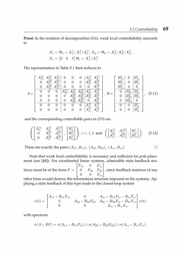
5.2 Controllability 69
Proof. In the notation of decomposition (5.6), weak local controllability amountsto
X1 = R1 = X11 +X2
1 +X31 , X2 = R2 = X1
2 +X22 +X3
2 ,
Xc =[0 0 I
]Rc = X1
c +X2c .
The representation in Table 5.1 then reduces to
A=
A1111 A12
11 A1311 0 0 0 A11
1c A121c
0 A2211 A23
11 0 0 0 A211c A22
1c
0 A3211 A33
11 0 0 0 0 A321c
0 0 0 A1122 A12
22 A1322 A11
2c A122c
0 0 0 0 A2222 A23
22 A212c A22
2c
0 0 0 0 A3222 A33
22 0 A322c
0 0 0 0 0 0 A11cc A12
cc
0 0 0 0 0 0 A21cc A22
cc
, B=
B111 0 B1
1c
B211 0 B2
1c
B311 0 00 B1
22 B12c
0 B222 B2
2c
0 B322 0
0 0 B1cc
0 0 B2cc
, (5.11)
and the corresponding controllable pairs in (5.9) areA11ii A12
ii A13ii
0 A22ii A23
ii
0 A32ii A33
ii
,B1
ii
B2ii
B3ii
, i = 1, 2 and([A11cc A12
cc
A21cc A22
cc
],
[B1cc
B2cc
]). (5.12)
These are exactly the pairs (A11, B11), (A22, B22), (Acc, Bcc).
Note that weak local controllability is necessary and sufficient for pole place-ment (see [48]): For coordinated linear systems, admissible state feedback ma-
trices must be of the form F =
F11 0 F1c
0 F22 F2c
0 0 Fcc
, since feedback matrices of any
other form would destroy the information structure imposed on the systems. Ap-plying a state feedback of this type leads to the closed-loop system
x(t) =
A11 + B11F11 0 A1c + B11F1c + B1cFcc0 A22 + B22F22 A2c + B22F2c + B2cFcc0 0 Acc + BccFcc
x(t),
with spectrum
σ(A + BF ) = σ(A11 + B11F11) ∪ σ(A22 + B22F22) ∪ σ(Acc + BccFcc).
70 Chapter 5: Controllability and Observability
Now the spectrum of the closed-loop system matrix can be assigned freely if andonly if the pairs (A11, B11), (A22, B22) and (Acc, Bcc) are controllable pairs, andthis is equivalent to weak local controllability of the coordinated linear system.
5.2.3.3 Strong local controllability
The concept of strong local controllability will be defined as follows:
5.2.13. Definition. We call a system of the form (5.1) strongly locally control-lable if for i = 1, 2, all states xi ∈ Xi are ui-reachable, and for all xc ∈ Xc, the state 0
0xc
is uc-reachable, i.e. if
R1 = X1, R2 = X2 and Rc ∩Xc = Xc.
An important detail in this definition is that for all xc ∈ Xc,
00xc
is uc-reachable:
For weak local controllability we only require that for all xc ∈ Xc there exist
x1 ∈ X1 and x2 ∈ X2 such that
x1
x2
xc
is reachable, but these x1 and x2 may depend
on the value of xc.The difference between the concepts of weak and strong local controllability
is that in the case of strong local controllability, it is possible to control each partof the system locally and independently, i.e. without influencing the rest of thesystem (see Remark 5.2.5). This means that control synthesis can be done in afully decentralized manner: As in the case of weak local controllability, each partof the system can be controlled locally. In contrast to weak local controllability,control synthesis for the subsystems can be done in such a way that the subsystemstate at a fixed time t is not influenced by the coordinator.
To illustrate this independence, we outline the control synthesis procedure fora strongly locally controllable system: Suppose we want the system to reach the
state
x1
x2
xc
at time t, from the initial state
000
at time 0. This can be done as
follows:
• Fix input trajectories u1 : [0, t] → U1 and u2 : [0, t] → U2 such that the localsystems described by
x1 = A11x1 + B11u1, x1(0) = 0,
x2 = A22x2 + B22u2, x2(0) = 0,
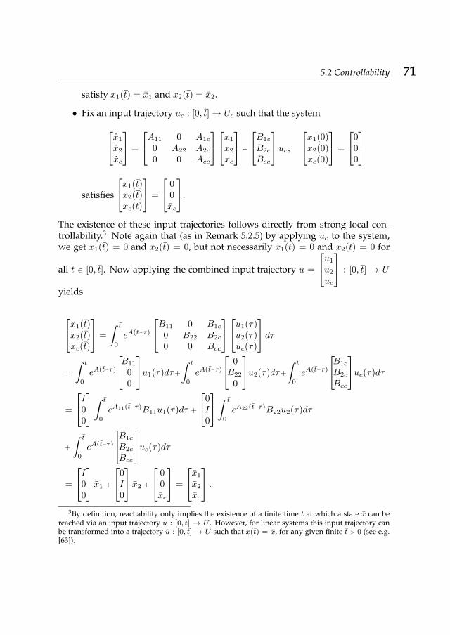
5.2 Controllability 71
satisfy x1(t) = x1 and x2(t) = x2.
• Fix an input trajectory uc : [0, t]→ Uc such that the systemx1
x2
xc
=
A11 0 A1c
0 A22 A2c
0 0 Acc
x1
x2
xc
+
B1c
B2c
Bcc
uc,x1(0)x2(0)xc(0)
=
000
satisfies
x1(t)x2(t)xc(t)
=
00xc
.
The existence of these input trajectories follows directly from strong local con-trollability.3 Note again that (as in Remark 5.2.5) by applying uc to the system,we get x1(t) = 0 and x2(t) = 0, but not necessarily x1(t) = 0 and x2(t) = 0 for
all t ∈ [0, t]. Now applying the combined input trajectory u =
u1
u2
uc
: [0, t] → U
yields
x1(t)x2(t)xc(t)
=
∫ t
0
eA(t−τ)
B11 0 B1c
0 B22 B2c
0 0 Bcc
u1(τ)u2(τ)uc(τ)
dτ=
∫ t
0
eA(t−τ)
B11
00
u1(τ)dτ+
∫ t
0
eA(t−τ)
0B22
0
u2(τ)dτ+
∫ t
0
eA(t−τ)
B1c
B2c
Bcc
uc(τ)dτ
=
I00
∫ t
0
eA11(t−τ)B11u1(τ)dτ +
0I0
∫ t
0
eA22(t−τ)B22u2(τ)dτ
+
∫ t
0
eA(t−τ)
B1c
B2c
Bcc
uc(τ)dτ
=
I00
x1 +
0I0
x2 +
00xc
=
x1
x2
xc
.3By definition, reachability only implies the existence of a finite time t at which a state x can be
reached via an input trajectory u : [0, t] → U . However, for linear systems this input trajectory canbe transformed into a trajectory u : [0, t] → U such that x(t) = x, for any given finite t > 0 (see e.g.[63]).
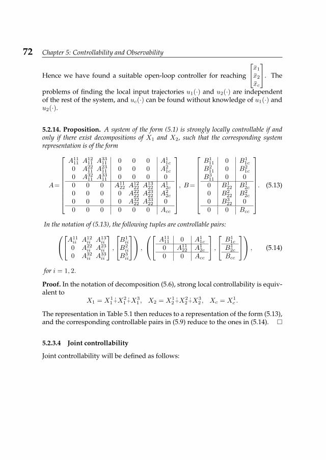
72 Chapter 5: Controllability and Observability
Hence we have found a suitable open-loop controller for reaching
x1
x2
xc
. The
problems of finding the local input trajectories u1(·) and u2(·) are independentof the rest of the system, and uc(·) can be found without knowledge of u1(·) andu2(·).
5.2.14. Proposition. A system of the form (5.1) is strongly locally controllable if andonly if there exist decompositions of X1 and X2, such that the corresponding systemrepresentation is of the form
A=
A1111 A12
11 A3311 0 0 0 A1
1c
0 A2211 A23
11 0 0 0 A21c
0 A3211 A33
11 0 0 0 00 0 0 A11
22 A1222 A13
22 A12c
0 0 0 0 A2222 A23
22 A22c
0 0 0 0 A3222 A33
22 00 0 0 0 0 0 Acc
, B=
B111 0 B1
1c
B211 0 B2
1c
B311 0 00 B1
22 B12c
0 B222 B2
2c
0 B322 0
0 0 Bcc
. (5.13)
In the notation of (5.13), the following tuples are controllable pairs:A11ii A12
ii A13ii
0 A22ii A23
ii
0 A32ii A33
ii
,B1
ii
B2ii
B3ii
,
A1111 0 A1
1c
0 A1122 A1
2c
0 0 Acc
, B1
1c
B12c
Bcc
, (5.14)
for i = 1, 2.
Proof. In the notation of decomposition (5.6), strong local controllability is equiv-alent to
X1 = X11 +X2
1 +X31 , X2 = X1
2 +X22 +X3
2 , Xc = X1c .
The representation in Table 5.1 then reduces to a representation of the form (5.13),and the corresponding controllable pairs in (5.9) reduce to the ones in (5.14).
5.2.3.4 Joint controllability
Joint controllability will be defined as follows:
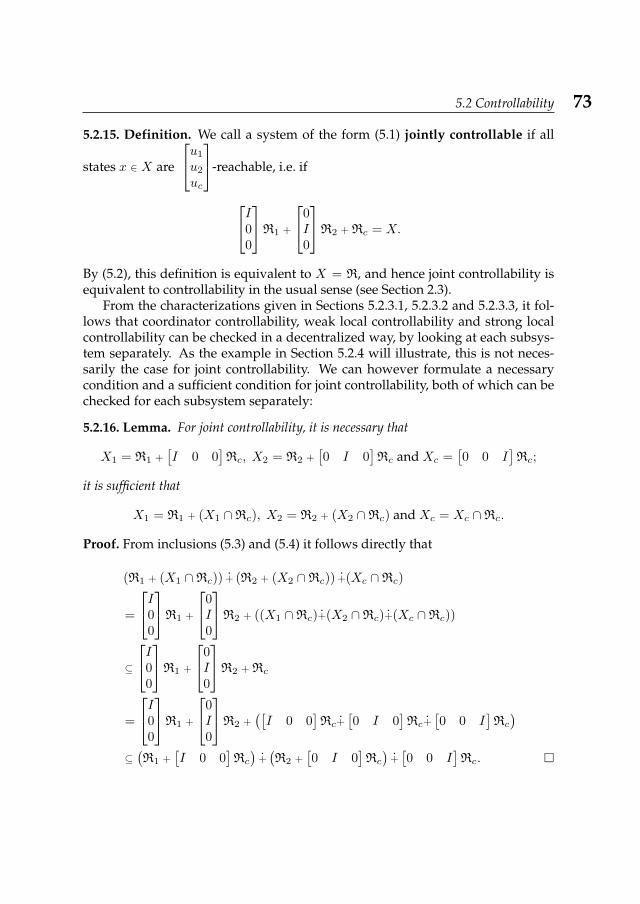
5.2 Controllability 73
5.2.15. Definition. We call a system of the form (5.1) jointly controllable if all
states x ∈ X are
u1
u2
uc
-reachable, i.e. if
I00
R1 +
0I0
R2 + Rc = X.
By (5.2), this definition is equivalent to X = R, and hence joint controllability isequivalent to controllability in the usual sense (see Section 2.3).
From the characterizations given in Sections 5.2.3.1, 5.2.3.2 and 5.2.3.3, it fol-lows that coordinator controllability, weak local controllability and strong localcontrollability can be checked in a decentralized way, by looking at each subsys-tem separately. As the example in Section 5.2.4 will illustrate, this is not neces-sarily the case for joint controllability. We can however formulate a necessarycondition and a sufficient condition for joint controllability, both of which can bechecked for each subsystem separately:
5.2.16. Lemma. For joint controllability, it is necessary that
X1 = R1 +[I 0 0
]Rc, X2 = R2 +
[0 I 0
]Rc and Xc =
[0 0 I
]Rc;
it is sufficient that
X1 = R1 + (X1 ∩Rc), X2 = R2 + (X2 ∩Rc) and Xc = Xc ∩Rc.
Proof. From inclusions (5.3) and (5.4) it follows directly that
(R1 + (X1 ∩Rc)) + (R2 + (X2 ∩Rc)) +(Xc ∩Rc)
=
I00
R1 +
0I0
R2 + ((X1 ∩Rc)+(X2 ∩Rc)+(Xc ∩Rc))
⊆
I00
R1 +
0I0
R2 + Rc
=
I00
R1 +
0I0
R2 +([I 0 0
]Rc+
[0 I 0
]Rc+
[0 0 I
]Rc
)⊆(R1 +
[I 0 0
]Rc
)+(R2 +
[0 I 0
]Rc
)+[0 0 I
]Rc.
74 Chapter 5: Controllability and Observability
For coordinated linear systems, joint controllability is not a very natural con-cept: If the sufficient condition is not satisfied then control requires some parts ofthe system to reverse the effects caused by controlling other parts of the system;
if, for example, Rc = span
III
then the state
00xc
can only be reached by
an input trajectory
u1(·)u2(·)uc(·)
, where neither u1(·) nor u2(·) can be identically zero.
Since for the subsystems, both the initial state and the target state are zero, theonly purpose of the non-zero input trajectories is to counteract the influence ofthe coordinator on the subsystems.
5.2.3.5 Independent controllability
A more natural concept for coordinated linear systems is independent controlla-bility, which will be defined as follows:
5.2.17. Definition. We call a system of the form (5.1) independently controllable
if for all x1 ∈ X1 the state
x1
00
is[u1
uc
]-reachable, for all x2 ∈ X2 the state
0x2
0
is
[u2
uc
]-reachable, and for all xc ∈ Xc the state
00xc
is uc-reachable, i.e. if
(R1 + (X1 ∩Rc)) + (R2 + (X2 ∩Rc)) +(Xc ∩Rc) = X.
In the case of independent controllability, each part of the system can be con-trolled in such a way that at a finite time t, no other part of the system is influ-enced by that control signal (see Remark 5.2.5). Control is possible both via thelocal inputs and the coordinator input. As is immediate from Definition 5.2.17,independent controllability coincides with the sufficient condition for joint con-trollability, and hence can be checked by looking at each part of the system sepa-rately.
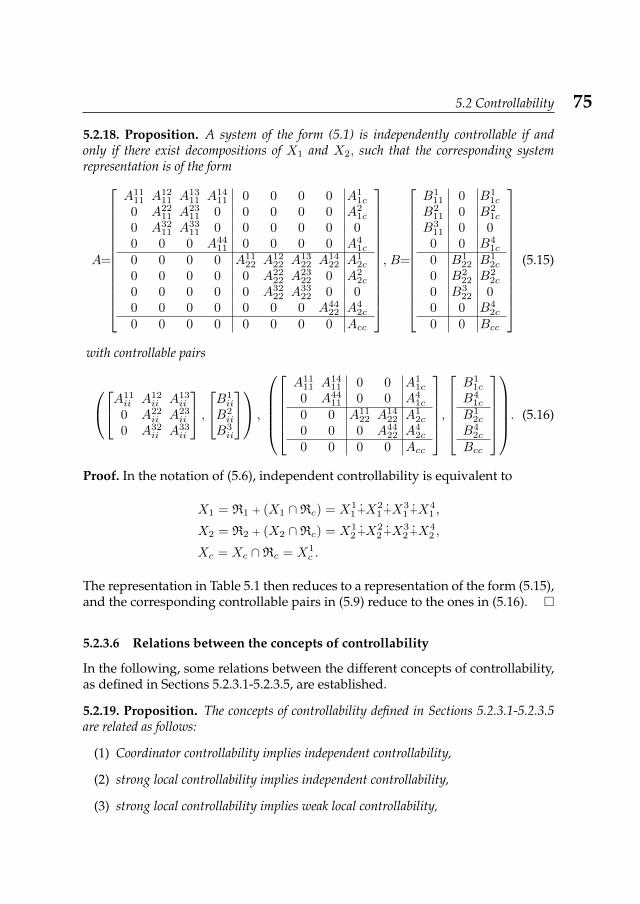
5.2 Controllability 75
5.2.18. Proposition. A system of the form (5.1) is independently controllable if andonly if there exist decompositions of X1 and X2, such that the corresponding systemrepresentation is of the form
A=
A1111 A12
11 A1311 A14
11 0 0 0 0 A11c
0 A2211 A23
11 0 0 0 0 0 A21c
0 A3211 A33
11 0 0 0 0 0 00 0 0 A44
11 0 0 0 0 A41c
0 0 0 0 A1122 A12
22 A1322 A14
22 A12c
0 0 0 0 0 A2222 A23
22 0 A22c
0 0 0 0 0 A3222 A33
22 0 00 0 0 0 0 0 0 A44
22 A42c
0 0 0 0 0 0 0 0 Acc
, B=
B111 0 B1
1c
B211 0 B2
1c
B311 0 00 0 B4
1c
0 B122 B1
2c
0 B222 B2
2c
0 B322 0
0 0 B42c
0 0 Bcc
(5.15)
with controllable pairs
A11ii A12
ii A13ii
0 A22ii A23
ii
0 A32ii A33
ii
,B1
ii
B2ii
B3ii
,
A11
11 A1411 0 0 A1
1c
0 A4411 0 0 A4
1c
0 0 A1122 A14
22 A12c
0 0 0 A4422 A4
2c
0 0 0 0 Acc
,B1
1c
B41c
B12c
B42c
Bcc
. (5.16)
Proof. In the notation of (5.6), independent controllability is equivalent to
X1 = R1 + (X1 ∩Rc) = X11 +X2
1 +X31 +X4
1 ,
X2 = R2 + (X2 ∩Rc) = X12 +X2
2 +X32 +X4
2 ,
Xc = Xc ∩Rc = X1c .
The representation in Table 5.1 then reduces to a representation of the form (5.15),and the corresponding controllable pairs in (5.9) reduce to the ones in (5.16).
5.2.3.6 Relations between the concepts of controllability
In the following, some relations between the different concepts of controllability,as defined in Sections 5.2.3.1-5.2.3.5, are established.
5.2.19. Proposition. The concepts of controllability defined in Sections 5.2.3.1-5.2.3.5are related as follows:
(1) Coordinator controllability implies independent controllability,
(2) strong local controllability implies independent controllability,
(3) strong local controllability implies weak local controllability,
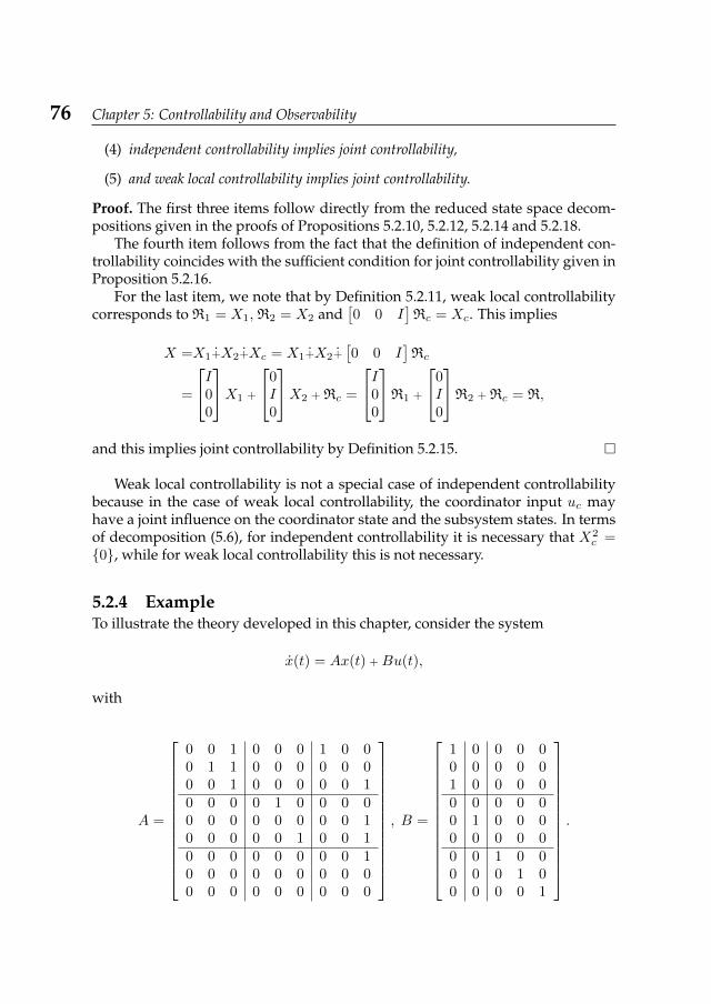
76 Chapter 5: Controllability and Observability
(4) independent controllability implies joint controllability,
(5) and weak local controllability implies joint controllability.
Proof. The first three items follow directly from the reduced state space decom-positions given in the proofs of Propositions 5.2.10, 5.2.12, 5.2.14 and 5.2.18.
The fourth item follows from the fact that the definition of independent con-trollability coincides with the sufficient condition for joint controllability given inProposition 5.2.16.
For the last item, we note that by Definition 5.2.11, weak local controllabilitycorresponds to R1 = X1, R2 = X2 and
[0 0 I
]Rc = Xc. This implies
X =X1+X2+Xc = X1+X2+[0 0 I
]Rc
=
I00
X1 +
0I0
X2 + Rc =
I00
R1 +
0I0
R2 + Rc = R,
and this implies joint controllability by Definition 5.2.15.
Weak local controllability is not a special case of independent controllabilitybecause in the case of weak local controllability, the coordinator input uc mayhave a joint influence on the coordinator state and the subsystem states. In termsof decomposition (5.6), for independent controllability it is necessary that X2
c =0, while for weak local controllability this is not necessary.
5.2.4 ExampleTo illustrate the theory developed in this chapter, consider the system
x(t) = Ax(t) + Bu(t),
with
A =
0 0 1 0 0 0 1 0 00 1 1 0 0 0 0 0 00 0 1 0 0 0 0 0 10 0 0 0 1 0 0 0 00 0 0 0 0 0 0 0 10 0 0 0 0 1 0 0 10 0 0 0 0 0 0 0 10 0 0 0 0 0 0 0 00 0 0 0 0 0 0 0 0
, B =
1 0 0 0 00 0 0 0 01 0 0 0 00 0 0 0 00 1 0 0 00 0 0 0 00 0 1 0 00 0 0 1 00 0 0 0 1
.
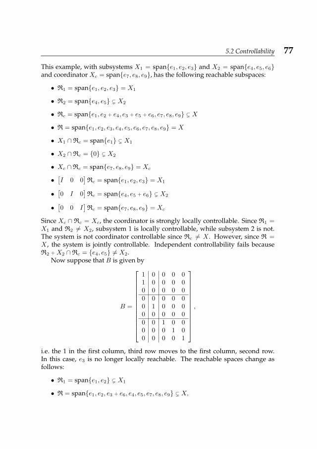
5.2 Controllability 77
This example, with subsystems X1 = spane1, e2, e3 and X2 = spane4, e5, e6and coordinator Xc = spane7, e8, e9, has the following reachable subspaces:
• R1 = spane1, e2, e3 = X1
• R2 = spane4, e5 ( X2
• Rc = spane1, e2 + e4, e3 + e5 + e6, e7, e8, e9 ( X
• R = spane1, e2, e3, e4, e5, e6, e7, e8, e9 = X
• X1 ∩Rc = spane1 ( X1
• X2 ∩Rc = 0 ( X2
• Xc ∩Rc = spane7, e8, e9 = Xc
•[I 0 0
]Rc = spane1, e2, e3 = X1
•[0 I 0
]Rc = spane4, e5 + e6 ( X2
•[0 0 I
]Rc = spane7, e8, e9 = Xc
Since Xc ∩Rc = Xc, the coordinator is strongly locally controllable. Since R1 =X1 and R2 6= X2, subsystem 1 is locally controllable, while subsystem 2 is not.The system is not coordinator controllable since Rc 6= X . However, since R =X , the system is jointly controllable. Independent controllability fails becauseR2 + X2 ∩Rc = e4, e5 6= X2.
Now suppose that B is given by
B =
1 0 0 0 01 0 0 0 00 0 0 0 00 0 0 0 00 1 0 0 00 0 0 0 00 0 1 0 00 0 0 1 00 0 0 0 1
,
i.e. the 1 in the first column, third row moves to the first column, second row.In this case, e3 is no longer locally reachable. The reachable spaces change asfollows:
• R1 = spane1, e2 ( X1
• R = spane1, e2, e3 + e6, e4, e5, e7, e8, e9 ( X,
78 Chapter 5: Controllability and Observability
The other subspaces stay the same. Now R 6= X , and hence the system is nolonger jointly controllable.
Note that for this example, controllability cannot be checked by looking at thesubsystems separately: For both choices of B, the sufficient condition of Lemma5.2.16 is not satisfied, but the necessary condition holds.
5.3 ObservabilityIn this section we consider coordinated linear systems without inputs and withoutputs, i.e. systems of the form
x(t) =
A11 0 A1c
0 A22 A2c
0 0 Acc
x(t),
y(t) =
C11 0 C1c
0 C22 C2c
0 0 Ccc
x(t),
(5.17)
with x(t) =
x1(t)x2(t)xc(t)
and y(t) =
y1(t)y2(t)yc(t)
.
In the following, we will refine the usual concept of indistinguishability, asdiscussed in Section 2.3, taking into account which output can distinguish a statefrom the zero state, and which part of the system the distinguishable state be-longs to. Based on these new concepts, we will derive an observability decompo-sition for coordinated linear systems, and introduce several possible concepts ofobservability for systems of the form (5.17).
5.3.1 IndistinguishabilityFor the case of unstructured linear systems, the concept of indistinguishabilitydescribes whether a given initial state can be distinguished from the zero initialstate via the output trajectory in finite time (see e.g. [21]).
For coordinated linear systems, it is not only relevant whether a state is indis-tinguishable from the zero state, but also which output is able or unable to distin-guish this state from 0. Since for coordinated linear systems we have CXi ⊆ Yi,the state xi of subsystem i can possibly be observed by looking at the correspond-ing local output yi, while xi is indistinguishable from 0 at the other subsystem orthe coordinator. However, the state xc of the coordinator system may be distin-guishable from 0 at y1, y2 or yc. In order to separate these different cases, weintroduce the following refined concepts of indistinguishability:
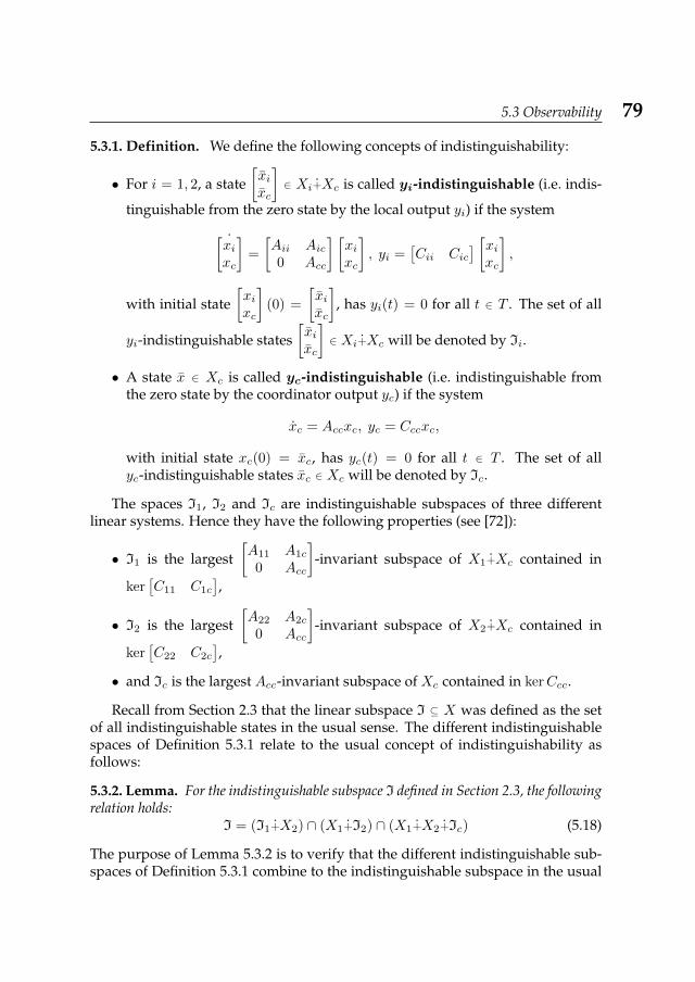
5.3 Observability 79
5.3.1. Definition. We define the following concepts of indistinguishability:
• For i = 1, 2, a state[xixc
]∈ Xi+Xc is called yi-indistinguishable (i.e. indis-
tinguishable from the zero state by the local output yi) if the system
˙[xixc
]=
[Aii Aic0 Acc
] [xixc
], yi =
[Cii Cic
] [xixc
],
with initial state[xixc
](0) =
[xixc
], has yi(t) = 0 for all t ∈ T . The set of all
yi-indistinguishable states[xixc
]∈ Xi+Xc will be denoted by Ii.
• A state x ∈ Xc is called yc-indistinguishable (i.e. indistinguishable fromthe zero state by the coordinator output yc) if the system
xc = Accxc, yc = Cccxc,
with initial state xc(0) = xc, has yc(t) = 0 for all t ∈ T . The set of allyc-indistinguishable states xc ∈ Xc will be denoted by Ic.
The spaces I1, I2 and Ic are indistinguishable subspaces of three differentlinear systems. Hence they have the following properties (see [72]):
• I1 is the largest[A11 A1c
0 Acc
]-invariant subspace of X1+Xc contained in
ker[C11 C1c
],
• I2 is the largest[A22 A2c
0 Acc
]-invariant subspace of X2+Xc contained in
ker[C22 C2c
],
• and Ic is the largest Acc-invariant subspace of Xc contained in kerCcc.
Recall from Section 2.3 that the linear subspace I ⊆ X was defined as the setof all indistinguishable states in the usual sense. The different indistinguishablespaces of Definition 5.3.1 relate to the usual concept of indistinguishability asfollows:
5.3.2. Lemma. For the indistinguishable subspace I defined in Section 2.3, the followingrelation holds:
I = (I1+X2) ∩ (X1+I2) ∩ (X1+X2+Ic) (5.18)
The purpose of Lemma 5.3.2 is to verify that the different indistinguishable sub-spaces of Definition 5.3.1 combine to the indistinguishable subspace in the usual
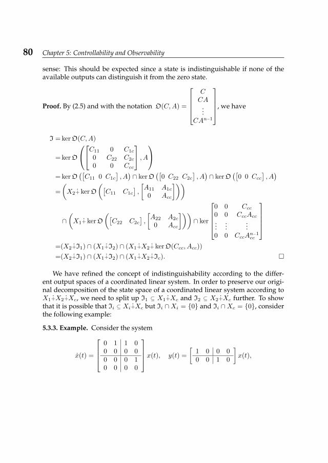
80 Chapter 5: Controllability and Observability
sense: This should be expected since a state is indistinguishable if none of theavailable outputs can distinguish it from the zero state.
Proof. By (2.5) and with the notation O(C,A) =
CCA
...CAn−1
, we have
I = kerO(C,A)
= kerO
C11 0 C1c
0 C22 C2c
0 0 Ccc
, A
= kerO([C11 0 C1c
], A)∩ kerO
([0 C22 C2c
], A)∩ kerO
([0 0 Ccc
], A)
=
(X2+ kerO
([C11 C1c
],
[A11 A1c
0 Acc
]))
∩(X1+ kerO
([C22 C2c
],
[A22 A2c
0 Acc
]))∩ ker
0 0 Ccc0 0 CccAcc...
......
0 0 CccAn−1cc
=(X2+I1) ∩ (X1+I2) ∩ (X1+X2+ kerO(Ccc, Acc))
=(X2+I1) ∩ (X1+I2) ∩ (X1+X2+Ic).
We have refined the concept of indistinguishability according to the differ-ent output spaces of a coordinated linear system. In order to preserve our origi-nal decomposition of the state space of a coordinated linear system according toX1+X2+Xc, we need to split up I1 ⊆ X1+Xc and I2 ⊆ X2+Xc further. To showthat it is possible that Ii ⊆ Xi+Xc but Ii ∩Xi = 0 and Ii ∩Xc = 0, considerthe following example:
5.3.3. Example. Consider the system
x(t) =
0 1 1 00 0 0 00 0 0 10 0 0 0
x(t), y(t) =
[1 0 0 00 0 1 0
]x(t),
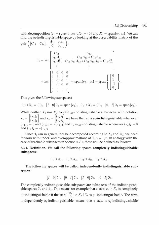
5.3 Observability 81
with decomposition X1 = spane1, e2, X2 = 0 and Xc = spane3, e4. We canfind the y1-indistinguishable space by looking at the observability matrix of the
pair([C11 C1c
],
[A11 A1c
0 Acc
]):
I1 = ker
C11 C1c
C11A11 C11A1c + C1cAccC11A
211 C11A11A1c + C11A1cAcc + C1cA
2cc
......
= ker
1 0 0 00 1 1 00 0 0 10 0 0 0...
......
...
= spane2 − e3 = span
01−10
.
This gives the following subspaces:
I1 ∩X1 = 0,[I 0
]I1 = spane2, I1 ∩Xc = 0,
[0 I
]I1 = spane3.
While neither X1 nor Xc contain y1-indistinguishable subspaces, with notation
x1 =
[(x1)1
(x1)2
]and xc =
[(xc)1
(xc)2
]we have that x1 is y1-indistinguishable whenever
(x1)1 = 0 and (xc)1 = −(x1)2, and xc is y1-indistinguishable whenever (xc)2 = 0and (x1)2 = −(xc)1.
Since Ii can in general not be decomposed according to Xi and Xc, we needto work with under- and overapproximations of Ii, i = 1, 2. In analogy with thecase of reachable subspaces in Section 5.2.1, these will be defined as follows:
5.3.4. Definition. We call the following spaces completely indistinguishablesubspaces:
I1 ∩X1, I1 ∩Xc, I2 ∩X2, I2 ∩Xc.
The following spaces will be called independently indistinguishable sub-spaces: [
I 0]I1,
[0 I
]I1,
[I 0
]I2,
[0 I
]I2.
The completely indistinguishable subspaces are subspaces of the indistinguish-able spaces I1 and I2. This means for example that a state x1 ∈ X1 is completely
y1-indistinguishable if the state[x1
0
]∈ X1+Xc is y1-indistinguishable. The term
‘independently yj-indistinguishable’ means that a state is yj-indistinguishable
82 Chapter 5: Controllability and Observability
from 0 if no further information from the other outputs is available: A statex1 ∈ X1 is independently y1-indistinguishable if there exists a state xc ∈ Xc such
that[x1
xc
]is yi-indistinguishable. However, xc might not be 0, so it is possible that
xc is observable from y2 or yc, and given the value of xc we may be able to derivethe value of x1. In other words, a state is independently yj-indistinguishable if itis not distinguishable from 0 by the output yj alone.
It immediately follows that
(Ii ∩Xi) + (Ii ∩Xc) ⊆ Ii ⊆[I 0
]Ii+
[0 I
]Ii,
and hence by (5.18), we have
(I1 ∩X1) + (I2 ∩X2) + ((I1 ∩Xc) ∩ (I2 ∩Xc) ∩ Ic) ⊆ I, (5.19)
I ⊆[I 0
]I1+
[I 0
]I2+
([0 I
]I1 ∩
[0 I
]I2 ∩ Ic
). (5.20)
5.3.2 Observability decompositionWe will decompose the state space X according to the observability properties ofthe system, by first decomposing X1+Xc, and then including X2 in the decompo-sition. In the following, we call a subspace of the state space yj-distinguishable ifit contains no non-zero yj-indistinguishable states.
In Xi, i = 1, 2, we have the yi-indistinguishable subspaces Ii ∩ Xi and[I 0
]Ii, with Ii ∩Xi ⊆
[I 0
]Ii. Hence, we can decompose Xi as follows:
5.3.5. Procedure.
(1) Let X3i = Ii ∩Xi.
(2) Let X2i be any complement of X3
i in[I 0
]Ii.
(3) Finally, let X1i be any complement of X2
i +X3i in Xi.
Now Xi = X1i +X2
i +X3i , with the following distinguishability properties:
subspace yi-distinguishableX1i yes
X2i depends on xc
X3i no
For the decomposition of Xc according to the observability properties of thesystem corresponding to Xi+Xc, we have to take into account the indistinguish-able subspaces Ic, Ii ∩Xc and
[0 I
]Ii, with Ii ∩Xc ⊆
[0 I
]Ii. We decompose
Xc as follows:
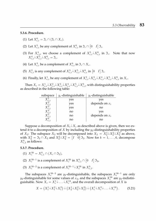
5.3 Observability 83
5.3.6. Procedure.
(1) Let X6c,i = Ic ∩ (Ii ∩Xc).
(2) Let X5c,i be any complement of X6
c,i in Ic ∩[0 I
]Ii.
(3) For X4c,i, we choose a complement of X5
c,i+X6c,i in Ic. Note that now
X4c,i+X
5c,i+X
6c,i = Ic.
(4) Let X3c,i be a complement of X6
c,i in Ii ∩Xc.
(5) X2c,i is any complement of X3
c,i+X5c,i+X
6c,i in
[0 I
]Ii.
(6) Finally, let X1c,i be any complement of X2
c,i+X3c,i+X
4c,i+X
5c,i+X
6c,i in Xc.
Then Xc = X1c,i+X
2c,i+X
3c,i+X
4c,i+X
5c,i+X
6c,i, with distinguishability properties
as described in the following table:
subspace yc-distinguishable yi-distinguishableX1c,i yes yes
X2c,i yes depends on xi
X3c,i yes no
X4c,i no yes
X5c,i no depends on xi
X6c,i no no
Suppose a decomposition of X1+Xc as described above is given, then we ex-tend it to a decomposition of X by including the y2-distinguishability propertiesof X2: The subspace X2 will be decomposed into X2 = X1
2 +X22 +X3
2 as above,with X3
2 = I2 ∩ X2 and X22 +X3
2 =[I 0
]I2. Now for k = 1, . . . , 6, decompose
Xkc,1 as follows:
5.3.7. Procedure.
(1) X3kc = Xk
c,1 ∩ (Xc ∩ I2),
(2) X3k−1c is a complement of X3k
c in Xkc,1 ∩
[0 I
]I2,
(3) X3k−2c is a complement of X3k−1
c +X3kc in Xk
c,1.
The subspaces X3k−2c are y2-distinguishable, the subspaces X3k−1
c are onlyy2-distinguishable for some values of x2, and the subspaces X3k
c are y2-indistin-guishable. Now Xc = X1
c + . . . +X18c , and the overall decomposition of X is
X =(X1
1 +X21 +X3
1
)+(X1
2 +X22 +X3
2
)+(X1c +X2
c + . . . +X18c
). (5.21)
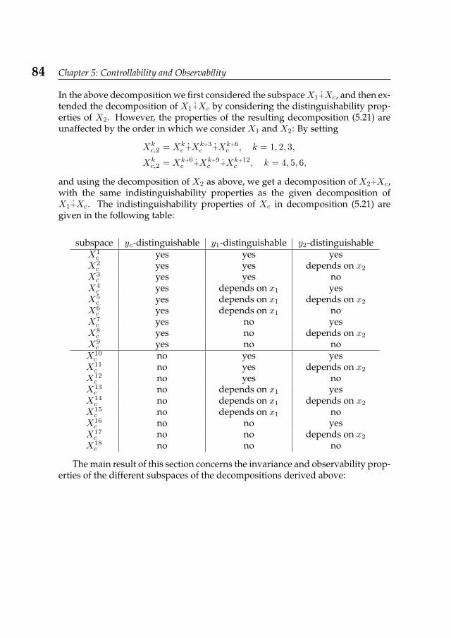
84 Chapter 5: Controllability and Observability
In the above decomposition we first considered the subspaceX1+Xc, and then ex-tended the decomposition of X1+Xc by considering the distinguishability prop-erties of X2. However, the properties of the resulting decomposition (5.21) areunaffected by the order in which we consider X1 and X2: By setting
Xkc,2 = Xk
c +Xk+3c +Xk+6
c , k = 1, 2, 3,
Xkc,2 = Xk+6
c +Xk+9c +Xk+12
c , k = 4, 5, 6,
and using the decomposition of X2 as above, we get a decomposition of X2+Xc,with the same indistinguishability properties as the given decomposition ofX1+Xc. The indistinguishability properties of Xc in decomposition (5.21) aregiven in the following table:
subspace yc-distinguishable y1-distinguishable y2-distinguishableX1c yes yes yes
X2c yes yes depends on x2
X3c yes yes no
X4c yes depends on x1 yes
X5c yes depends on x1 depends on x2
X6c yes depends on x1 no
X7c yes no yes
X8c yes no depends on x2
X9c yes no no
X10c no yes yes
X11c no yes depends on x2
X12c no yes no
X13c no depends on x1 yes
X14c no depends on x1 depends on x2
X15c no depends on x1 no
X16c no no yes
X17c no no depends on x2
X18c no no no
The main result of this section concerns the invariance and observability prop-erties of the different subspaces of the decompositions derived above:
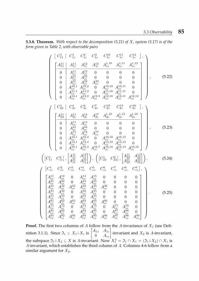
5.3 Observability 85
5.3.8. Theorem. With respect to the decomposition (5.21) of X , system (5.17) is of theform given in Table 2, with observable pairs
[C1
11 C11c C2
1c C31c C10
1c C111c C12
1c
],
A1111 A11
1c A121c A13
1c A1,101c A1,11
1c A1,121c
0 A11cc A12
cc 0 0 0 00 A21
cc A22cc 0 0 0 0
0 A31cc A32
cc A33cc 0 0 0
0 A10,1cc A10,2
cc 0 A10,10cc A10,11
cc 00 A11,1
cc A11,2cc 0 A11,10
cc A11,11cc 0
0 A12,1cc A12,2
cc A12,3cc A12,10
cc A12,11cc A12,12
cc
, (5.22)
[C1
22 C12c C4
2c C72c C10
2c C132c C16
2c
],
A1122 A11
2c A142c A17
2c A1,102c A1,13
2c A1,162c
0 A11cc A14
cc 0 0 0 00 A41
cc A44cc 0 0 0 0
0 A71cc A74
cc A77cc 0 0 0
0 A10,1cc A10,4
cc 0 A10,10cc A10,13
cc 00 A13,1
cc A13,4cc 0 A13,10
cc A13,13cc 0
0 A16,1cc A16,4
cc A16,7cc A16,10
cc A16,13cc A16,16
cc
, (5.23)
([C1
11 C211
],
[A11
11 A1211
A2111 A22
11
]),
([C1
22 C222
],
[A11
22 A1222
A2122 A22
22
]), (5.24)
[C1cc C2
cc C3cc C4
cc C5cc C6
cc C7cc C8
cc C9cc
],
A11cc A12
cc 0 A14cc A15
cc 0 0 0 0A21cc A22
cc 0 A24cc A25
cc 0 0 0 0A31cc A32
cc A33cc A34
cc A35cc A36
cc 0 0 0A41cc A42
cc 0 A44cc A45
cc 0 0 0 0A51cc A52
cc 0 A54cc A55
cc 0 0 0 0A61cc A62
cc A63cc A64
cc A65cc A66
cc 0 0 0A71cc A72
cc 0 A74cc A75
cc 0 A77cc A78
cc 0A81cc A82
cc 0 A84cc A85
cc 0 A87cc A88
cc 0A91cc A92
cc A93cc A94
cc A95cc A96
cc A97cc A98
cc A99cc
. (5.25)
Proof. The first two columns of A follow from the A-invariance of X1 (see Defi-
nition 3.1.1). Since I1 ⊆ X1+Xc is[A11 A1c
0 Acc
]-invariant and X2 is A-invariant,
the subspace I1+X2 ⊆ X is A-invariant. Now X31 = I1 ∩ X1 = (I1+X2) ∩ X1 is
A-invariant, which establishes the third column of A. Columns 4-6 follow from asimilar argument for X2.
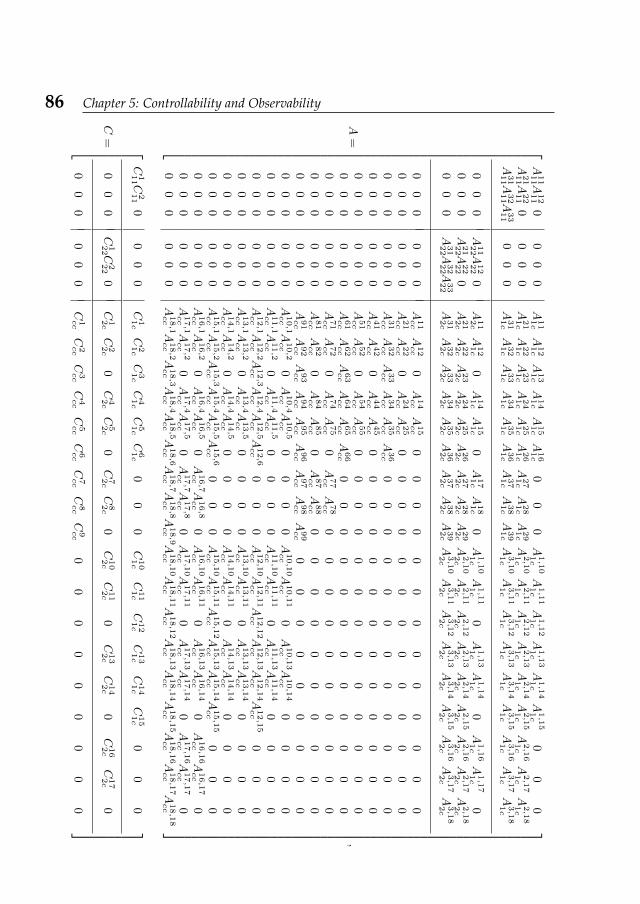
86 Chapter 5: Controllability and Observability
Table5.2:The
observabilitydecom
position
A=
A11
11 A
12
110
00
0A
11
1c
A12
1c
A13
1c
A14
1c
A15
1c
A16
1c
00
0A
1,10
1c
A1,11
1c
A1,12
1c
A1,13
1c
A1,14
1c
A1,15
1c
00
0
A21
11 A
22
110
00
0A
21
1c
A22
1c
A23
1c
A24
1c
A25
1c
A26
1c
A27
1c
A28
1c
A29
1cA
2,10
1c
A2,11
1c
A2,12
1c
A2,13
1c
A2,14
1c
A2,15
1c
A2,16
1c
A2,17
1c
A2,18
1c
A31
11 A
32
11 A
33
11
00
0A
31
1c
A32
1c
A33
1c
A34
1c
A35
1c
A36
1c
A37
1c
A38
1c
A39
1cA
3,10
1c
A3,11
1c
A3,12
1c
A3,13
1c
A3,14
1c
A3,15
1c
A3,16
1c
A3,17
1c
A3,18
1c
00
0A
11
22 A
12
220
A11
2c
A12
1c
0A
14
1c
A15
1c
0A
17
1c
A18
1c
0A
1,10
1c
A1,11
1c
0A
1,13
1c
A1,14
1c
0A
1,16
1c
A1,17
1c
0
00
0A
21
22 A
22
220
A21
2c
A22
2c
A23
2c
A24
2c
A25
2c
A26
2c
A27
2c
A28
2c
A29
2cA
2,10
2c
A2,11
2c
A2,12
2c
A2,13
2c
A2,14
2c
A2,15
2c
A2,16
2c
A2,17
2c
A2,18
2c
00
0A
31
22 A
32
22 A
33
22
A31
2c
A32
2c
A33
2c
A34
2c
A35
2c
A36
2c
A37
2c
A38
2c
A39
2cA
3,10
2c
A3,11
2c
A3,12
2c
A3,13
2c
A3,14
2c
A3,15
2c
A3,16
2c
A3,17
2c
A3,18
2c
00
00
00
A11cc
A12cc
0A
14cc
A15cc
00
00
00
00
00
00
00
00
00
0A
21cc
A22cc
0A
24cc
A25cc
00
00
00
00
00
00
00
00
00
0A
31cc
A32cc
A33cc
A34cc
A35cc
A36cc
00
00
00
00
00
00
00
00
00
A41cc
A42cc
0A
44cc
A45cc
00
00
00
00
00
00
00
00
00
0A
51cc
A52cc
0A
54cc
A55cc
00
00
00
00
00
00
00
00
00
0A
61cc
A62cc
A63cc
A64cc
A65cc
A66cc
00
00
00
00
00
00
00
00
00
A71cc
A72cc
0A
74cc
A75cc
0A
77cc
A78cc
00
00
00
00
00
00
00
00
A81cc
A82cc
0A
84cc
A85cc
0A
87cc
A88cc
00
00
00
00
00
00
00
00
A91cc
A92cc
A93cc
A94cc
A95cc
A96cc
A97cc
A98cc
A99cc
00
00
00
00
00
00
00
0A
10,1
cc
A10,2
cc
0A
10,4
cc
A10,5
cc
00
00
A10,10
cc
A10,11
cc
0A
10,13
cc
A10,14
cc
00
00
00
00
00
A11,1
cc
A11,2
cc
0A
11,4
cc
A11,5
cc
00
00
A11,10
cc
A11,11
cc
0A
11,13
cc
A11,14
cc
00
00
00
00
00
A12,1
cc
A12,2
cc
A12,3
cc
A12,4
cc
A12,5
cc
A12,6
cc
00
0A
12,10
cc
A12,11
cc
A12,12
cc
A12,13
cc
A12,14
cc
A12,15
cc
00
00
00
00
0A
13,1
cc
A13,2
cc
0A
13,4
cc
A13,5
cc
00
00
A13,10
cc
A13,11
cc
0A
13,13
cc
A13,14
cc
00
00
00
00
00
A14,1
cc
A14,2
cc
0A
14,4
cc
A14,5
cc
00
00
A14,10
cc
A14,11
cc
0A
14,13
cc
A14,14
cc
00
00
00
00
00
A15,1
cc
A15,2
cc
A15,3
cc
A15,4
cc
A15,5
cc
A15,6
cc
00
0A
15,10
cc
A15,11
cc
A15,12
cc
A15,13
cc
A15,14
cc
A15,15
cc
00
00
00
00
0A
16,1
cc
A16,2
cc
0A
16,4
cc
A16,5
cc
0A
16,7
cc
A16,8
cc
0A
16,10
cc
A16,11
cc
0A
16,13
cc
A16,14
cc
0A
16,16
cc
A16,17
cc
00
00
00
0A
17,1
cc
A17,2
cc
0A
17,4
cc
A17,5
cc
0A
17,7
cc
A17,8
cc
0A
17,10
cc
A17,11
cc
0A
17,13
cc
A17,14
cc
0A
17,16
cc
A17,17
cc
00
00
00
0A
18,1
cc
A18,2
cc
A18,3
cc
A18,4
cc
A18,5
cc
A18,6
cc
A18,7
cc
A18,8
cc
A18,9
cc
A18,10
cc
A18,11
cc
A18,12
cc
A18,13
cc
A18,14
cc
A18,15
cc
A18,16
cc
A18,17
cc
A18,18
cc
,
C=
C111 C
2110
00
0C
11c
C21c
C31c
C41c
C51c
C61c
00
0C
10
1c
C11
1c
C12
1c
C13
1c
C14
1c
C15
1c
00
0
00
0C
122 C
2220
C12c
C22c
0C
42c
C52c
0C
72c
C82c
0C
10
2c
C11
2c
0C
13
2c
C14
2c
0C
16
2c
C17
2c
0
00
00
00
C1cc
C2cc
C3cc
C4cc
C5cc
C6cc
C7cc
C8cc
C9cc
00
00
00
00
0
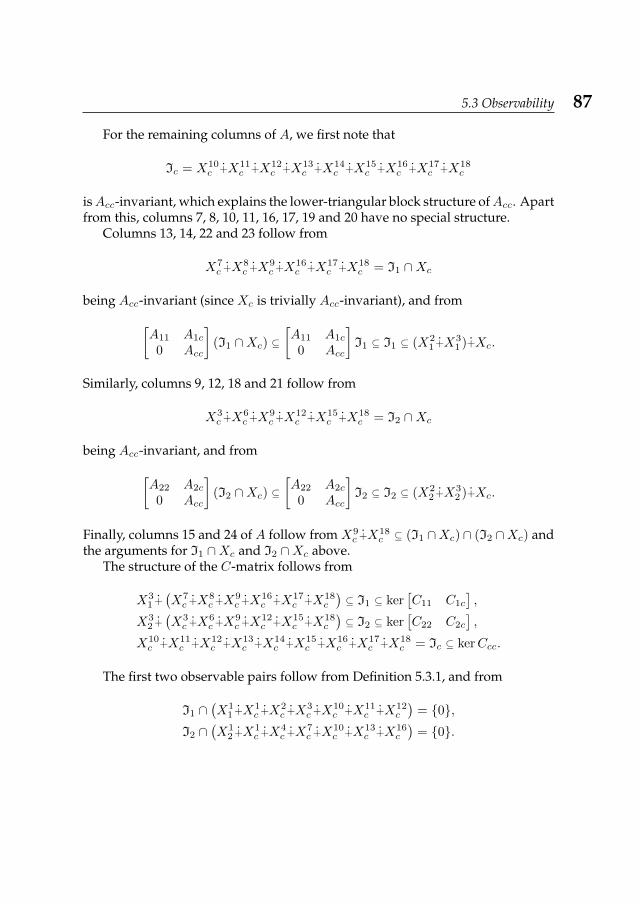
5.3 Observability 87
For the remaining columns of A, we first note that
Ic = X10c +X11
c +X12c +X13
c +X14c +X15
c +X16c +X17
c +X18c
isAcc-invariant, which explains the lower-triangular block structure ofAcc. Apartfrom this, columns 7, 8, 10, 11, 16, 17, 19 and 20 have no special structure.
Columns 13, 14, 22 and 23 follow from
X7c +X8
c +X9c +X16
c +X17c +X18
c = I1 ∩Xc
being Acc-invariant (since Xc is trivially Acc-invariant), and from[A11 A1c
0 Acc
](I1 ∩Xc) ⊆
[A11 A1c
0 Acc
]I1 ⊆ I1 ⊆ (X2
1 +X31 )+Xc.
Similarly, columns 9, 12, 18 and 21 follow from
X3c +X6
c +X9c +X12
c +X15c +X18
c = I2 ∩Xc
being Acc-invariant, and from[A22 A2c
0 Acc
](I2 ∩Xc) ⊆
[A22 A2c
0 Acc
]I2 ⊆ I2 ⊆ (X2
2 +X32 )+Xc.
Finally, columns 15 and 24 of A follow from X9c +X18
c ⊆ (I1 ∩Xc) ∩ (I2 ∩Xc) andthe arguments for I1 ∩Xc and I2 ∩Xc above.
The structure of the C-matrix follows from
X31 +(X7c +X8
c +X9c +X16
c +X17c +X18
c
)⊆ I1 ⊆ ker
[C11 C1c
],
X32 +(X3c +X6
c +X9c +X12
c +X15c +X18
c
)⊆ I2 ⊆ ker
[C22 C2c
],
X10c +X11
c +X12c +X13
c +X14c +X15
c +X16c +X17
c +X18c = Ic ⊆ kerCcc.
The first two observable pairs follow from Definition 5.3.1, and from
I1 ∩(X1
1 +X1c +X2
c +X3c +X10
c +X11c +X12
c
)= 0,
I2 ∩(X1
2 +X1c +X4
c +X7c +X10
c +X13c +X16
c
)= 0.
88 Chapter 5: Controllability and Observability
The third and fourth observable pairs are due to
X3i =Ii ∩Xi = kerO
([Cii Cic
],
[Aii Aic0 Acc
])∩Xi = ker
Cii C1c
CiiAii ?CiiA
2ii ?
......
∩X1
= kerO(Cii, Aii), i = 1, 2,
and the last observable pair is due to
Ic = X10c +X11
c +X12c +X13
c +X14c +X15
c +X16c +X17
c +X18c .
An additional decomposition of the output spaces Y1 and Y2 of the subsys-tems, specifying which part of the output observes (part of) the local subsystemstate or the coordinator state, would induce some additional structure on the C-matrix. This is not considered here.
5.3.3 Concepts of observabilityIn this section, the observability decomposition derived in the previous sectionwill be used for the characterization of several possible concepts of observability.
In analogy to Section 3.3, the two concepts of observability most relevant forpractical purposes are weak local observability (Definition 5.3.11) and indepen-dent observability (Definition 5.3.17).
5.3.3.1 Subsystem observability
Subsystem observability will be defined as follows:
5.3.9. Definition. We call a system of the form (5.17) subsystem observable if for
i = 1, 2, all non-zero states[xixc
]∈ X1+Xc are yi-distinguishable, i.e. if Ii = 0.
Subsystem observability is a rather strong condition (see Proposition 5.3.19).It is a useful concept if one aims at constructing a coordinated system that is asdecentralized as possible: If the system is subsystem observable then the coor-dinator is both y1-observable and y2-observable. These observations can then beused for local control synthesis, as described in Section 5.4. On the other hand,if a coordinated system is not subsystem observable and if one aims at having acoordinator of minimal dimension, then all parts of the coordinator that are notboth y1-observable and y2-observable can be moved to a subsystem (see [23]).
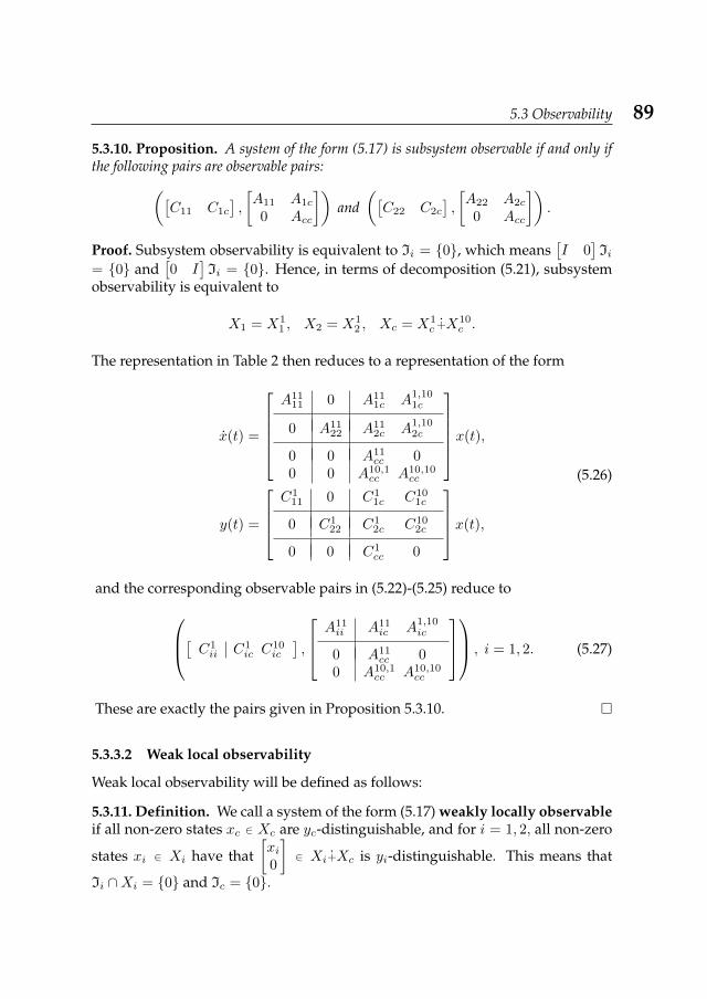
5.3 Observability 89
5.3.10. Proposition. A system of the form (5.17) is subsystem observable if and only ifthe following pairs are observable pairs:([
C11 C1c
],
[A11 A1c
0 Acc
])and
([C22 C2c
],
[A22 A2c
0 Acc
]).
Proof. Subsystem observability is equivalent to Ii = 0, which means[I 0
]Ii
= 0 and[0 I
]Ii = 0. Hence, in terms of decomposition (5.21), subsystem
observability is equivalent to
X1 = X11 , X2 = X1
2 , Xc = X1c +X10
c .
The representation in Table 2 then reduces to a representation of the form
x(t) =
A11
11 0 A111c A1,10
1c
0 A1122 A11
2c A1,102c
0 0 A11cc 0
0 0 A10,1cc A10,10
cc
x(t),
y(t) =
C1
11 0 C11c C10
1c
0 C122 C1
2c C102c
0 0 C1cc 0
x(t),
(5.26)
and the corresponding observable pairs in (5.22)-(5.25) reduce to[ C1ii C1
ic C10ic
],
A11ii A11
ic A1,10ic
0 A11cc 0
0 A10,1cc A10,10
cc
, i = 1, 2. (5.27)
These are exactly the pairs given in Proposition 5.3.10.
5.3.3.2 Weak local observability
Weak local observability will be defined as follows:
5.3.11. Definition. We call a system of the form (5.17) weakly locally observableif all non-zero states xc ∈ Xc are yc-distinguishable, and for i = 1, 2, all non-zero
states xi ∈ Xi have that[xi0
]∈ Xi+Xc is yi-distinguishable. This means that
Ii ∩Xi = 0 and Ic = 0.
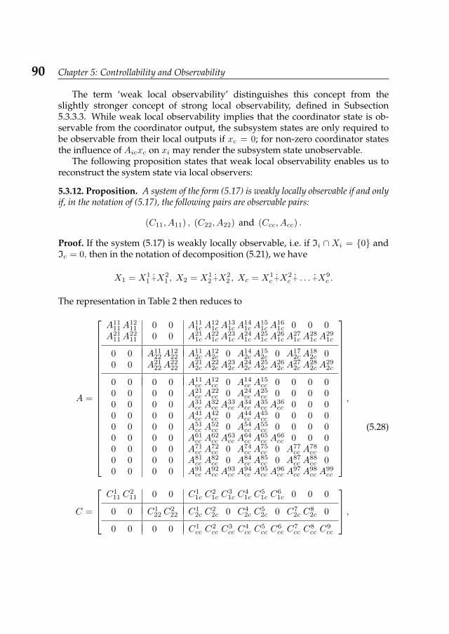
90 Chapter 5: Controllability and Observability
The term ‘weak local observability’ distinguishes this concept from theslightly stronger concept of strong local observability, defined in Subsection5.3.3.3. While weak local observability implies that the coordinator state is ob-servable from the coordinator output, the subsystem states are only required tobe observable from their local outputs if xc = 0; for non-zero coordinator statesthe influence of Aicxc on xi may render the subsystem state unobservable.
The following proposition states that weak local observability enables us toreconstruct the system state via local observers:
5.3.12. Proposition. A system of the form (5.17) is weakly locally observable if and onlyif, in the notation of (5.17), the following pairs are observable pairs:
(C11, A11) , (C22, A22) and (Ccc, Acc) .
Proof. If the system (5.17) is weakly locally observable, i.e. if Ii ∩ Xi = 0 andIc = 0, then in the notation of decomposition (5.21), we have
X1 = X11 +X2
1 , X2 = X12 +X2
2 , Xc = X1c +X2
c + . . . +X9c .
The representation in Table 2 then reduces to
A =
A1111A
1211 0 0 A11
1c A121c A
131c A
141c A
151c A
161c 0 0 0
A2111A
2211 0 0 A21
1c A221c A
231c A
241c A
251c A
261c A
271c A
281c A
291c
0 0 A1122A
1222 A11
2c A122c 0 A14
2c A152c 0 A17
2c A182c 0
0 0 A2122A
2222 A21
2c A222c A
232c A
242c A
252c A
262c A
272c A
282c A
292c
0 0 0 0 A11cc A
12cc 0 A14
cc A15cc 0 0 0 0
0 0 0 0 A21cc A
22cc 0 A24
cc A25cc 0 0 0 0
0 0 0 0 A31cc A
32cc A
33cc A
34cc A
35cc A
36cc 0 0 0
0 0 0 0 A41cc A
42cc 0 A44
cc A45cc 0 0 0 0
0 0 0 0 A51cc A
52cc 0 A54
cc A55cc 0 0 0 0
0 0 0 0 A61cc A
62cc A
63cc A
64cc A
65cc A
66cc 0 0 0
0 0 0 0 A71cc A
72cc 0 A74
cc A75cc 0 A77
cc A78cc 0
0 0 0 0 A81cc A
82cc 0 A84
cc A85cc 0 A87
cc A88cc 0
0 0 0 0 A91cc A
92cc A
93cc A
94cc A
95cc A
96cc A
97cc A
98cc A
99cc
,
C =
C1
11 C211 0 0 C1
1c C21c C
31c C
41c C
51c C
61c 0 0 0
0 0 C122 C
222 C1
2c C22c 0 C4
2c C52c 0 C7
2c C82c 0
0 0 0 0 C1cc C
2cc C
3cc C
4cc C
5cc C
6cc C
7cc C
8cc C
9cc
,
(5.28)
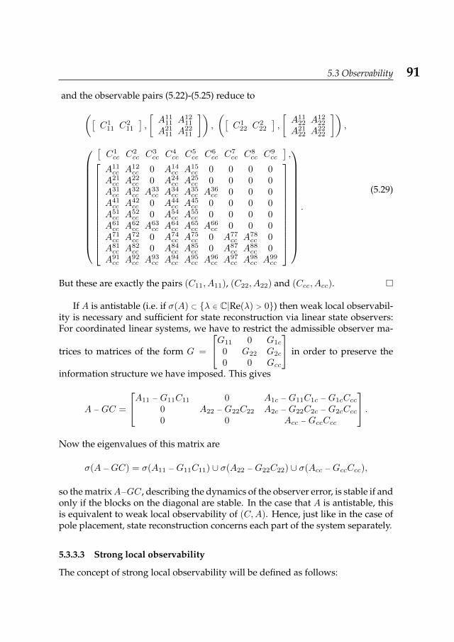
5.3 Observability 91
and the observable pairs (5.22)-(5.25) reduce to([C1
11 C211
],
[A11
11 A1211
A2111 A22
11
]),
([C1
22 C222
],
[A11
22 A1222
A2122 A22
22
]),
[C1cc C2
cc C3cc C4
cc C5cc C6
cc C7cc C8
cc C9cc
],
A11cc A12
cc 0 A14cc A15
cc 0 0 0 0A21cc A22
cc 0 A24cc A25
cc 0 0 0 0A31cc A32
cc A33cc A34
cc A35cc A36
cc 0 0 0A41cc A42
cc 0 A44cc A45
cc 0 0 0 0A51cc A52
cc 0 A54cc A55
cc 0 0 0 0A61cc A62
cc A63cc A64
cc A65cc A66
cc 0 0 0A71cc A72
cc 0 A74cc A75
cc 0 A77cc A78
cc 0A81cc A82
cc 0 A84cc A85
cc 0 A87cc A88
cc 0A91cc A92
cc A93cc A94
cc A95cc A96
cc A97cc A98
cc A99cc
.
(5.29)
But these are exactly the pairs (C11, A11), (C22, A22) and (Ccc, Acc).
If A is antistable (i.e. if σ(A) ⊂ λ ∈ C|Re(λ) > 0) then weak local observabil-ity is necessary and sufficient for state reconstruction via linear state observers:For coordinated linear systems, we have to restrict the admissible observer ma-
trices to matrices of the form G =
G11 0 G1c
0 G22 G2c
0 0 Gcc
in order to preserve the
information structure we have imposed. This gives
A −GC =
A11 −G11C11 0 A1c −G11C1c −G1cCcc0 A22 −G22C22 A2c −G22C2c −G2cCcc0 0 Acc −GccCcc
.Now the eigenvalues of this matrix are
σ(A −GC) = σ(A11 −G11C11) ∪ σ(A22 −G22C22) ∪ σ(Acc −GccCcc),
so the matrixA−GC, describing the dynamics of the observer error, is stable if andonly if the blocks on the diagonal are stable. In the case that A is antistable, thisis equivalent to weak local observability of (C,A). Hence, just like in the case ofpole placement, state reconstruction concerns each part of the system separately.
5.3.3.3 Strong local observability
The concept of strong local observability will be defined as follows:
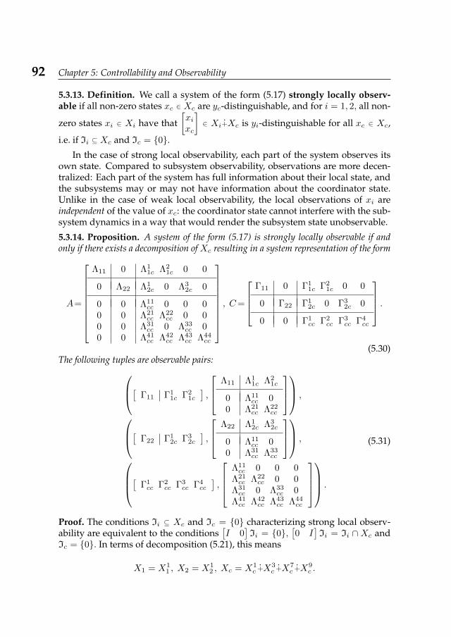
92 Chapter 5: Controllability and Observability
5.3.13. Definition. We call a system of the form (5.17) strongly locally observ-able if all non-zero states xc ∈ Xc are yc-distinguishable, and for i = 1, 2, all non-
zero states xi ∈ Xi have that[xixc
]∈ Xi+Xc is yi-distinguishable for all xc ∈ Xc,
i.e. if Ii ⊆ Xc and Ic = 0.In the case of strong local observability, each part of the system observes its
own state. Compared to subsystem observability, observations are more decen-tralized: Each part of the system has full information about their local state, andthe subsystems may or may not have information about the coordinator state.Unlike in the case of weak local observability, the local observations of xi areindependent of the value of xc: the coordinator state cannot interfere with the sub-system dynamics in a way that would render the subsystem state unobservable.
5.3.14. Proposition. A system of the form (5.17) is strongly locally observable if andonly if there exists a decomposition of Xc resulting in a system representation of the form
A=
Λ11 0 Λ11c Λ2
1c 0 0
0 Λ22 Λ12c 0 Λ3
2c 0
0 0 Λ11cc 0 0 0
0 0 Λ21cc Λ22
cc 0 00 0 Λ31
cc 0 Λ33cc 0
0 0 Λ41cc Λ42
cc Λ43cc Λ44
cc
, C=
Γ11 0 Γ1
1c Γ21c 0 0
0 Γ22 Γ12c 0 Γ3
2c 0
0 0 Γ1cc Γ2
cc Γ3cc Γ4
cc
.
(5.30)The following tuples are observable pairs:[ Γ11 Γ1
1c Γ21c
],
Λ11 Λ11c Λ2
1c
0 Λ11cc 0
0 Λ21cc Λ22
cc
,
[ Γ22 Γ12c Γ3
2c
],
Λ22 Λ12c Λ3
2c
0 Λ11cc 0
0 Λ31cc Λ33
cc
,
[ Γ1cc Γ2
cc Γ3cc Γ4
cc
],
Λ11cc 0 0 0
Λ21cc Λ22
cc 0 0Λ31cc 0 Λ33
cc 0Λ41cc Λ42
cc Λ43cc Λ44
cc
.
(5.31)
Proof. The conditions Ii ⊆ Xc and Ic = 0 characterizing strong local observ-ability are equivalent to the conditions
[I 0
]Ii = 0,
[0 I
]Ii = Ii ∩ Xc and
Ic = 0. In terms of decomposition (5.21), this means
X1 = X11 , X2 = X1
2 , Xc = X1c +X3
c +X7c +X9
c .
5.3 Observability 93
The representation in Table 2 then reduces to a representation of the form (5.30),and the corresponding observable pairs in (5.22)-(5.25) reduce to the ones in(5.31).
An interesting generalization of both subsystem observability and strong localobservability is to require that for some matrices D1c, D2c and Dcc of appropriate
sizes,[I 00 D1c
] [x1
xc
]is observable at subsystem 1,
[I 00 D2c
] [x2
xc
]is observable
at subsystem 2, and Dccxc is observable at the coordinator. The interpretationof this concept is that each subsystem observes, in addition to its own state, aparticular part of the coordinator state. The observable part of the coordinatorcan be different for each subsystem.
This concept is equivalent to Ii ⊆ kerDic for i = 1, 2, and Ic ⊆ kerDcc. Forsubsystem observability, we have Dic = I, i = 1, 2 and Dcc = 0. Strong localobservability corresponds to the other extreme, with Dic = 0 for i = 1, 2, andDcc = I .
5.3.3.4 Joint observability
We define joint observability as follows:
5.3.15. Definition. We call a system of the form (5.17) jointly observable if all
non-zero states x ∈ X are
y1
y2
yc
-distinguishable, i.e. if
(I1+X2) ∩ (I2+X1) ∩ (Ic+X1+X2) = 0.
Since the characterization of joint observability is equivalent to I = 0 byLemma 5.3.2, the concept of joint observability coincides with the usual conceptof observability. For coordinated linear systems, this concept is not very useful: Ifthe system is jointly observable but not independently observable (see Definition5.3.17), then the overall state of the system can only be observed by combining theobservations of the different parts of the system; the combination of these obser-vations requires communication among different parts of the system, which doesnot comply with the information structure we imposed on coordinated systems.This difficulty is illustrated by an example in Section 5.3.4.
Since the concept of joint observability cannot be characterized by separateconditions for each part of the system (which reflects the need for communicationbetween the different parts of the system for the observation of the system state),we cannot give a reduced decomposition for this concept. We can however givea necessary condition and a sufficient condition for joint observability, both ofwhich separate into conditions on the different parts of the system:
94 Chapter 5: Controllability and Observability
5.3.16. Lemma. For joint observability of a coordinated linear system of the form (5.17),and hence for observability in the usual sense, it is necessary that
I1 ∩X1 = 0, I2 ∩X2 = 0, (I1 ∩Xc) ∩ (I2 ∩Xc) ∩ Ic = 0;
it is sufficient that
I1 ⊆ Xc, I2 ⊆ Xc,[0 I
]I1 ∩
[0 I
]I2 ∩ Ic = 0.
Proof. The necessary condition follows directly from (5.19). For the sufficientcondition, note that[
I 0]I1 = 0,
[I 0
]I2 = 0,
[0 I
]I1 ∩
[0 I
]I2 ∩ Ic = 0
is sufficient for I = 0 by (5.20), but ([I 0
]Ii = 0)⇔ (Ii ⊆ Xc), which gives
the sufficient condition stated above.
5.3.3.5 Independent observability
Independent observability will be defined as follows:
5.3.17. Definition. We call a system of the form (5.17) independently observ-
able if all non-zero states xc ∈ Xc have that
x1
x2
xc
∈ X1+X2+Xc is
y1
y2
yc
-
distinguishable for any x1 ∈ X1 and x2 ∈ X2, and for i = 1, 2 all non-zero states
xi ∈ Xi have that the state[xixc
]∈ X1+Xc is yi-distinguishable for all xc ∈ Xc, i.e.
if [I 0
]Ii = 0, i = 1, 2,
[0 I
]I1 ∩
[0 I
]I2 ∩ Ic = 0.
By Lemma 5.3.16, independent observability coincides with the sufficient con-dition for joint observability. Hence it is a stronger condition than joint observ-ability, and more useful in the setting of coordinated linear systems because allparts of the system state are observable independently of the value of xc: no com-munication among the different parts of the system is required to observe thesubsystem states. The coordinator state can only be observed jointly by the dif-ferent outputs.
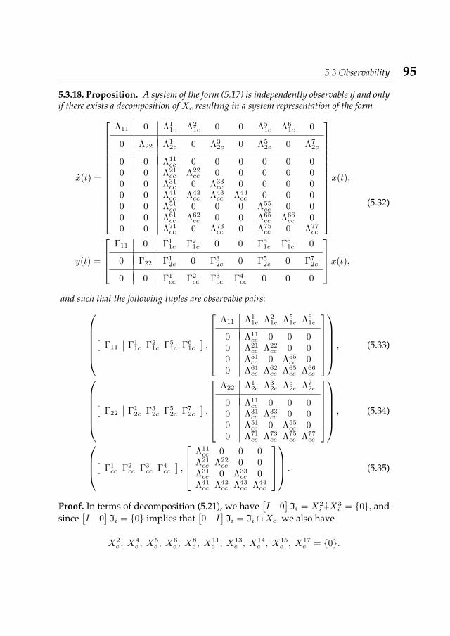
5.3 Observability 95
5.3.18. Proposition. A system of the form (5.17) is independently observable if and onlyif there exists a decomposition of Xc resulting in a system representation of the form
x(t) =
Λ11 0 Λ11c Λ2
1c 0 0 Λ51c Λ6
1c 0
0 Λ22 Λ12c 0 Λ3
2c 0 Λ52c 0 Λ7
2c
0 0 Λ11cc 0 0 0 0 0 0
0 0 Λ21cc Λ22
cc 0 0 0 0 00 0 Λ31
cc 0 Λ33cc 0 0 0 0
0 0 Λ41cc Λ42
cc Λ43cc Λ44
cc 0 0 00 0 Λ51
cc 0 0 0 Λ55cc 0 0
0 0 Λ61cc Λ62
cc 0 0 Λ65cc Λ66
cc 00 0 Λ71
cc 0 Λ73cc 0 Λ75
cc 0 Λ77cc
x(t),
y(t) =
Γ11 0 Γ1
1c Γ21c 0 0 Γ5
1c Γ61c 0
0 Γ22 Γ12c 0 Γ3
2c 0 Γ52c 0 Γ7
2c
0 0 Γ1cc Γ2
cc Γ3cc Γ4
cc 0 0 0
x(t),
(5.32)
and such that the following tuples are observable pairs:[
Γ11 Γ11c Γ2
1c Γ51c Γ6
1c
],
Λ11 Λ1
1c Λ21c Λ5
1c Λ61c
0 Λ11cc 0 0 0
0 Λ21cc Λ22
cc 0 00 Λ51
cc 0 Λ55cc 0
0 Λ61cc Λ62
cc Λ65cc Λ66
cc
, (5.33)
[
Γ22 Γ12c Γ3
2c Γ52c Γ7
2c
],
Λ22 Λ1
2c Λ32c Λ5
2c Λ72c
0 Λ11cc 0 0 0
0 Λ31cc Λ33
cc 0 00 Λ51
cc 0 Λ55cc 0
0 Λ71cc Λ73
cc Λ75cc Λ77
cc
, (5.34)
[ Γ1cc Γ2
cc Γ3cc Γ4
cc
],
Λ11cc 0 0 0
Λ21cc Λ22
cc 0 0Λ31cc 0 Λ33
cc 0Λ41cc Λ42
cc Λ43cc Λ44
cc
. (5.35)
Proof. In terms of decomposition (5.21), we have[I 0
]Ii = X2
i +X3i = 0, and
since[I 0
]Ii = 0 implies that
[0 I
]Ii = Ii ∩Xc, we also have
X2c , X
4c , X
5c , X
6c , X
8c , X
11c , X
13c , X
14c , X
15c , X
17c = 0.
96 Chapter 5: Controllability and Observability
Now the second condition for independent observability reduces to[0 I
]I1 ∩[
0 I]I2 ∩ Ic = X18
c = 0. Hence, independent observability is equivalent to
X1 = X11 , X2 = X1
2 , Xc = X1c +X3
c +X7c +X9
c +X10c +X12
c +X16c .
The representation in Table then reduces to a representation of the form (5.32),and the corresponding observable pairs in (5.22)-(5.25) reduce to the ones in(5.33)-(5.35).
5.3.3.6 Relations between the concepts of observability
For the different concepts of observability defined in Sections 5.3.3.1-5.3.3.5, wehave the following relations:
5.3.19. Proposition.
• Subsystem observability implies independent observability,
• strong local observability implies independent observability,
• strong local observability implies weak local observability,
• independent observability implies joint observability,
• and weak local observability implies joint observability.
Proof. The first three items follow directly from the reduced state space decom-positions given in the proofs of Propositions 5.3.10, 5.3.12, 5.3.14 and 5.3.18.
The definition of independent observability in 5.3.17 coincides with the suffi-cient condition for joint observability in 5.3.16, which gives the fourth item.
Weak local observability corresponds to Ii∩Xi = 0 for i = 1, 2 and Ic = 0by Definition 5.3.11, and since
I = (I1+X2) ∩ (I2+X1) ∩ (Ic+X1+X2)
= (I1+X2) ∩ (I2+X1) ∩ (X1+X2)
= ((I1 ∩X1)+X2) ∩ ((I2 ∩X2)+X1) = X2 ∩X1 = 0,
this implies joint observability by Definition 5.3.15.
In the case of weak local observability, the observability of the subsystemstates xi might depend on the value of xc, and hence the observability proper-ties of the subsystem states are not independent of the rest of the system. Henceweak local observability is not a special case of independent observability.
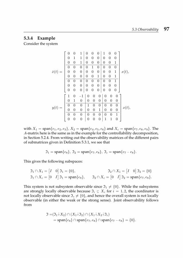
5.3 Observability 97
5.3.4 ExampleConsider the system
x(t) =
0 0 1 0 0 0 1 0 00 1 1 0 0 0 0 0 00 0 1 0 0 0 0 0 10 0 0 0 1 0 0 0 00 0 0 0 0 0 0 0 10 0 0 0 0 1 0 0 10 0 0 0 0 0 0 0 10 0 0 0 0 0 0 0 00 0 0 0 0 0 0 0 0
x(t),
y(t) =
1 0 −1 0 0 0 0 0 00 1 0 0 0 0 0 0 00 0 0 1 0 0 0 0 00 0 0 0 0 1 0 0 00 0 0 0 0 0 0 0 10 0 0 0 0 0 1 1 0
x(t),
with X1 = spane1, e2, e3, X2 = spane4, e5, e6 and Xc = spane7, e8, e9. TheA-matrix here is the same as in the example for the controllability decomposition,in Section 5.2.4. From writing out the observability matrices of the different pairsof submatrices given in Definition 5.3.1, we see that
I1 = spane8, I2 = spane7, e8, Ic = spane7 − e8.
This gives the following subspaces:
I1 ∩X1 =[I 0
]I1 = 0, I2 ∩X1 =
[I 0
]I2 = 0
I1 ∩Xc =[0 I
]I1 = spane8, I2 ∩Xc =
[0 I
]I2 = spane7, e8.
This system is not subsystem observable since I1 6= 0. While the subsystemsare strongly locally observable because Ii ⊆ Xc for i = 1, 2, the coordinator isnot locally observable since Ic 6= 0, and hence the overall system is not locallyobservable (in either the weak or the strong sense). Joint observability followsfrom
I =(I1+X2) ∩ (X1+I2) ∩ (X1+X2+Ic)
= spane8 ∩ spane7, e8 ∩ spane7 − e8 = 0.
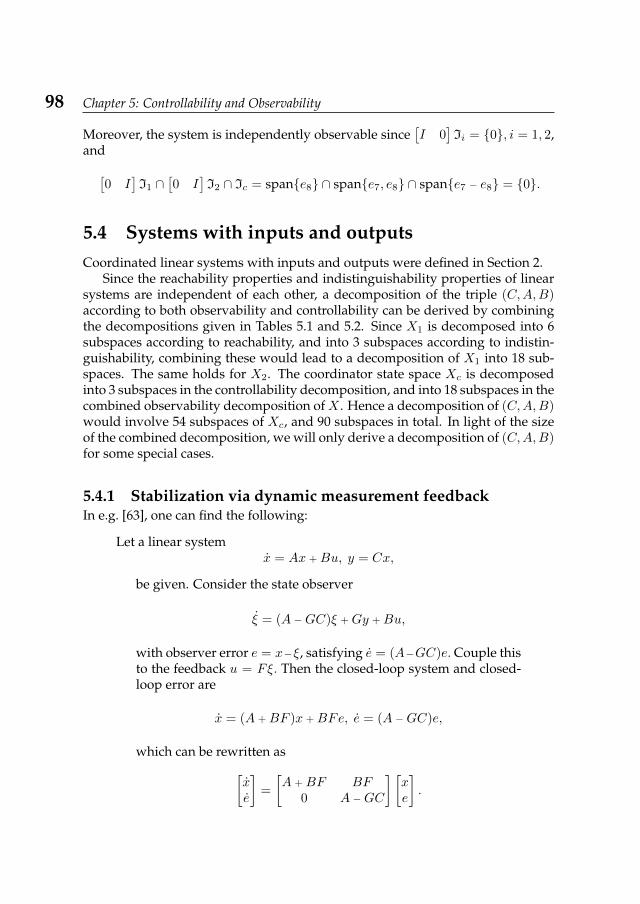
98 Chapter 5: Controllability and Observability
Moreover, the system is independently observable since[I 0
]Ii = 0, i = 1, 2,
and[0 I
]I1 ∩
[0 I
]I2 ∩ Ic = spane8 ∩ spane7, e8 ∩ spane7 − e8 = 0.
5.4 Systems with inputs and outputsCoordinated linear systems with inputs and outputs were defined in Section 2.
Since the reachability properties and indistinguishability properties of linearsystems are independent of each other, a decomposition of the triple (C,A,B)according to both observability and controllability can be derived by combiningthe decompositions given in Tables 5.1 and 5.2. Since X1 is decomposed into 6subspaces according to reachability, and into 3 subspaces according to indistin-guishability, combining these would lead to a decomposition of X1 into 18 sub-spaces. The same holds for X2. The coordinator state space Xc is decomposedinto 3 subspaces in the controllability decomposition, and into 18 subspaces in thecombined observability decomposition ofX . Hence a decomposition of (C,A,B)would involve 54 subspaces of Xc, and 90 subspaces in total. In light of the sizeof the combined decomposition, we will only derive a decomposition of (C,A,B)for some special cases.
5.4.1 Stabilization via dynamic measurement feedbackIn e.g. [63], one can find the following:
Let a linear systemx = Ax + Bu, y = Cx,
be given. Consider the state observer
ξ = (A −GC)ξ + Gy + Bu,
with observer error e = x−ξ, satisfying e = (A−GC)e. Couple thisto the feedback u = Fξ. Then the closed-loop system and closed-loop error are
x = (A + BF )x + BFe, e = (A −GC)e,
which can be rewritten as[xe
]=
[A + BF BF
0 A −GC
] [xe
].
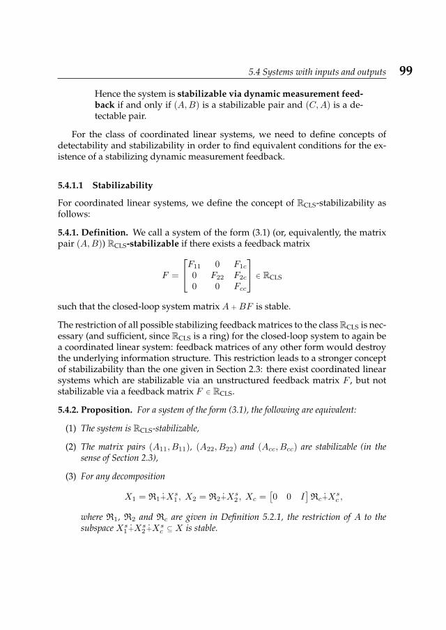
5.4 Systems with inputs and outputs 99
Hence the system is stabilizable via dynamic measurement feed-back if and only if (A,B) is a stabilizable pair and (C,A) is a de-tectable pair.
For the class of coordinated linear systems, we need to define concepts ofdetectability and stabilizability in order to find equivalent conditions for the ex-istence of a stabilizing dynamic measurement feedback.
5.4.1.1 Stabilizability
For coordinated linear systems, we define the concept of RCLS-stabilizability asfollows:
5.4.1. Definition. We call a system of the form (3.1) (or, equivalently, the matrixpair (A,B)) RCLS-stabilizable if there exists a feedback matrix
F =
F11 0 F1c
0 F22 F2c
0 0 Fcc
∈ RCLS
such that the closed-loop system matrix A + BF is stable.
The restriction of all possible stabilizing feedback matrices to the class RCLS is nec-essary (and sufficient, since RCLS is a ring) for the closed-loop system to again bea coordinated linear system: feedback matrices of any other form would destroythe underlying information structure. This restriction leads to a stronger conceptof stabilizability than the one given in Section 2.3: there exist coordinated linearsystems which are stabilizable via an unstructured feedback matrix F , but notstabilizable via a feedback matrix F ∈ RCLS.
5.4.2. Proposition. For a system of the form (3.1), the following are equivalent:
(1) The system is RCLS-stabilizable,
(2) The matrix pairs (A11, B11), (A22, B22) and (Acc, Bcc) are stabilizable (in thesense of Section 2.3),
(3) For any decomposition
X1 = R1+Xs1 , X2 = R2+Xs
2 , Xc =[0 0 I
]Rc+X
sc ,
where R1, R2 and Rc are given in Definition 5.2.1, the restriction of A to thesubspace Xs
1 +Xs2 +Xs
c ⊆ X is stable.
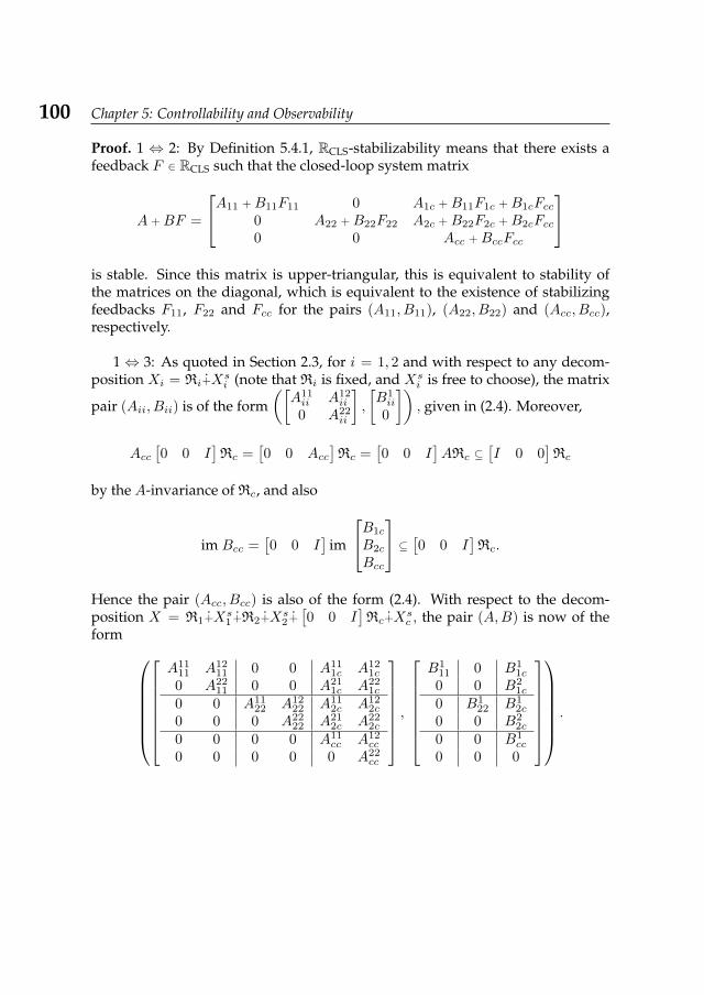
100 Chapter 5: Controllability and Observability
Proof. 1 ⇔ 2: By Definition 5.4.1, RCLS-stabilizability means that there exists afeedback F ∈ RCLS such that the closed-loop system matrix
A + BF =
A11 + B11F11 0 A1c + B11F1c + B1cFcc0 A22 + B22F22 A2c + B22F2c + B2cFcc0 0 Acc + BccFcc
is stable. Since this matrix is upper-triangular, this is equivalent to stability ofthe matrices on the diagonal, which is equivalent to the existence of stabilizingfeedbacks F11, F22 and Fcc for the pairs (A11, B11), (A22, B22) and (Acc, Bcc),respectively.
1 ⇔ 3: As quoted in Section 2.3, for i = 1, 2 and with respect to any decom-position Xi = Ri+X
si (note that Ri is fixed, and Xs
i is free to choose), the matrix
pair (Aii, Bii) is of the form([A11ii A12
ii
0 A22ii
],
[B1ii
0
]), given in (2.4). Moreover,
Acc[0 0 I
]Rc =
[0 0 Acc
]Rc =
[0 0 I
]ARc ⊆
[I 0 0
]Rc
by the A-invariance of Rc, and also
im Bcc =[0 0 I
]im
B1c
B2c
Bcc
⊆ [0 0 I]Rc.
Hence the pair (Acc, Bcc) is also of the form (2.4). With respect to the decom-position X = R1+Xs
1 +R2+Xs2 +[0 0 I
]Rc+X
sc , the pair (A,B) is now of the
form
A11
11 A1211 0 0 A11
1c A121c
0 A2211 0 0 A21
1c A221c
0 0 A1122 A12
22 A112c A12
2c
0 0 0 A2222 A21
2c A222c
0 0 0 0 A11cc A12
cc
0 0 0 0 0 A22cc
,B1
11 0 B11c
0 0 B21c
0 B122 B1
2c
0 0 B22c
0 0 B1cc
0 0 0
.
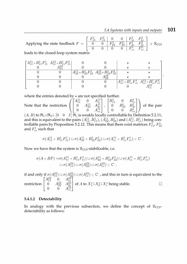
5.4 Systems with inputs and outputs 101
Applying the state feedback F =
F 111 F 2
11 0 0 F 11c F 2
1c
0 0 F 122 F 2
22 F 12c F 2
2c
0 0 0 0 F 1cc F 2
cc
∈ RCLS
leads to the closed-loop system matrixA11
11+B111F
111 A12
11+B111F
211 0 0 ? ?
0 A2211 0 0 ? ?
0 0 A1122+B1
22F122 A12
22+B122F
222 ? ?
0 0 0 A2222 ? ?
0 0 0 0 A11cc +B1
ccF1cc A
12cc +B1
ccF2cc
0 0 0 0 0 A22cc
,
where the entries denoted by ? are not specified further.
Note that the restriction
A1111 0 A11
1c
0 A1122 A11
2c
0 0 A11cc
,B1
11 0 B11c
0 B122 B1
2c
0 0 B1cc
of the pair
(A,B) to R1+R2+[0 0 I
]Rc is weakly locally controllable by Definition 5.2.11,
and this is equivalent to the pairs (A1111, B
111), (A11
22, B122) and (A11
cc , B1cc) being con-
trollable pairs by Proposition 5.2.12. This means that there exist matrices F 111, F 1
22
and F 1cc such that
σ(A1111 + B1
11F111) ∪ σ(A11
22 + B122F
122) ∪ σ(A11
cc + B1ccF
1cc) ⊂ C−.
Now we have that the system is RCLS-stabilizable, i.e.
σ(A + BF ) =σ(A1111 + B1
11F111) ∪ σ(A11
22 + B122F
122) ∪ σ(A11
cc + B1ccF
1cc)
∪ σ(A2211) ∪ σ(A22
22) ∪ σ(A22cc ) ⊂ C−,
if and only if σ(A2211) ∪ σ(A22
22) ∪ σ(A22cc ) ⊂ C−, and this in turn is equivalent to the
restriction
A2211 0 A22
1c
0 A2222 A22
2c
0 0 A22cc
of A to Xs1 +Xs
2 +Xsc being stable.
5.4.1.2 Detectability
In analogy with the previous subsection, we define the concept of RCLS-detectability as follows:
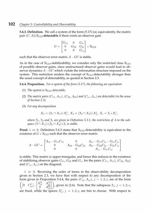
102 Chapter 5: Controllability and Observability
5.4.3. Definition. We call a system of the form (5.17) (or, equivalently, the matrixpair (C,A)) RCLS-detectable if there exists an observer gain
G =
G11 0 G1c
0 G22 G2c
0 0 Gcc
∈ RCLS
such that the observer error matrix A −GC is stable.
As in the case of RCLS-stabilizability, we consider only the restricted class RCLSof possible observer gains, since unstructured observer gains would lead to ob-server dynamics A −GC which violate the information structure imposed on thesystem. This restriction renders the concept of RCLS-detectability stronger thanthe usual concept of detectability, as quoted in Section 2.3.
5.4.4. Proposition. For a system of the form (5.17), the following are equivalent:
(1) The system is RCLS-detectable,
(2) The matrix pairs (C11, A11), (C22, A22) and (Ccc, Acc) are detectable (in the senseof Section 2.3),
(3) For any decomposition
X1 = (I1 ∩X1)+Xr1 , X2 = (I2 ∩X2)+Xr
2 , Xc = Ic+Xrc ,
where I1, I2 and Ic are given in Definition 5.3.1, the restriction of A to the sub-space (I ∩X1)+(I2 ∩X2)+Ic is stable.
Proof. 1 ⇔ 2: Definition 5.4.3 states that RCLS-detectability is equivalent to theexistence of G ∈ RCLS such that the observer error matrix
A −GC =
A11 −G11C11 0 A1c −G11C1c −G1cCcc0 A22 −G22C22 A2c −G22C2c −G2cCcc0 0 Acc −GccCcc
is stable. This matrix is upper-triangular, and hence this reduces to the existenceof stabilizing observer gains G11, G22 and Gcc for the pairs (C11, A11), (C22, A22)and (Ccc, Acc) on the diagonal.
1 ⇔ 3: Reversing the order of terms in the observability decompositiongiven in Section 2.3, we have that with respect to any decomposition of theform given in Proposition 5.4.4, the pairs (Cjj , Ajj), j = 1, 2, c, are of the form([
0 C2jj
],
[A11jj A12
jj
0 A22jj
]), given in (2.6). Note that the subspaces Ij , j = 1, 2, c,
are fixed, while the spaces Xrj , j = 1, 2, c, are free to choose. With respect to
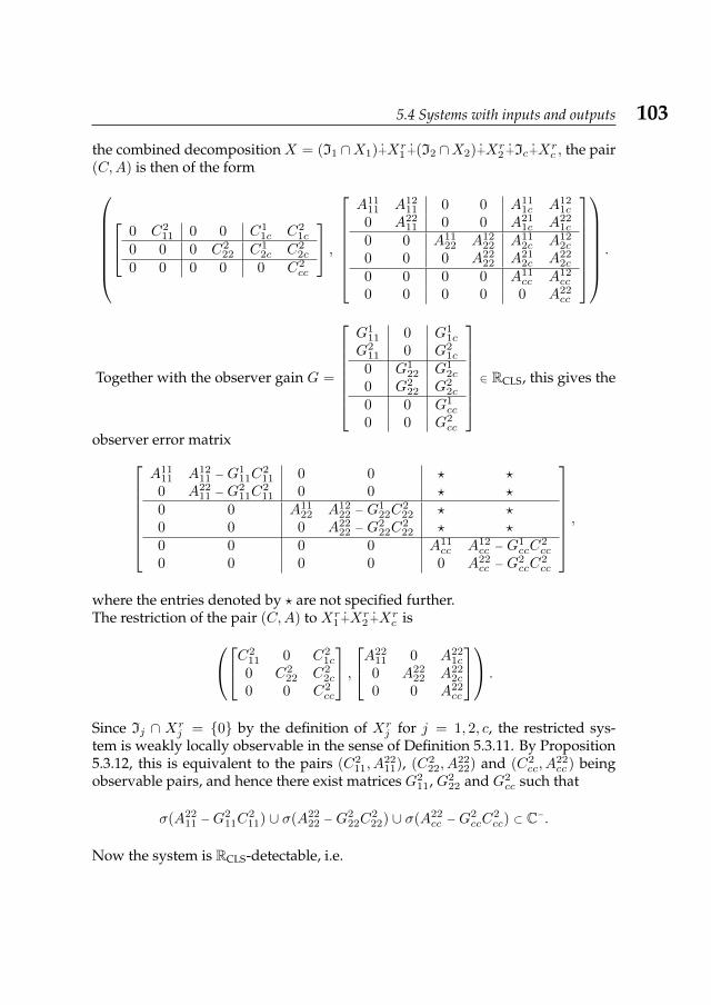
5.4 Systems with inputs and outputs 103
the combined decomposition X = (I1 ∩X1)+Xr1 +(I2 ∩X2)+Xr
2 +Ic+Xrc , the pair
(C,A) is then of the form 0 C2
11 0 0 C11c C2
1c
0 0 0 C222 C1
2c C22c
0 0 0 0 0 C2cc
,A11
11 A1211 0 0 A11
1c A121c
0 A2211 0 0 A21
1c A221c
0 0 A1122 A12
22 A112c A12
2c
0 0 0 A2222 A21
2c A222c
0 0 0 0 A11cc A12
cc
0 0 0 0 0 A22cc
.
Together with the observer gain G =
G1
11 0 G11c
G211 0 G2
1c
0 G122 G1
2c
0 G222 G2
2c
0 0 G1cc
0 0 G2cc
∈ RCLS, this gives the
observer error matrixA11
11 A1211 −G
111C
211 0 0 ? ?
0 A2211 −G
211C
211 0 0 ? ?
0 0 A1122 A12
22 −G122C
222 ? ?
0 0 0 A2222 −G
222C
222 ? ?
0 0 0 0 A11cc A12
cc −G1ccC
2cc
0 0 0 0 0 A22cc −G
2ccC
2cc
,
where the entries denoted by ? are not specified further.The restriction of the pair (C,A) to Xr
1 +Xr2 +Xr
c isC211 0 C2
1c
0 C222 C2
2c
0 0 C2cc
,A22
11 0 A221c
0 A2222 A22
2c
0 0 A22cc
.
Since Ij ∩ Xrj = 0 by the definition of Xr
j for j = 1, 2, c, the restricted sys-tem is weakly locally observable in the sense of Definition 5.3.11. By Proposition5.3.12, this is equivalent to the pairs (C2
11, A2211), (C2
22, A2222) and (C2
cc, A22cc ) being
observable pairs, and hence there exist matrices G211, G2
22 and G2cc such that
σ(A2211 −G
211C
211) ∪ σ(A22
22 −G222C
222) ∪ σ(A22
cc −G2ccC
2cc) ⊂ C−.
Now the system is RCLS-detectable, i.e.
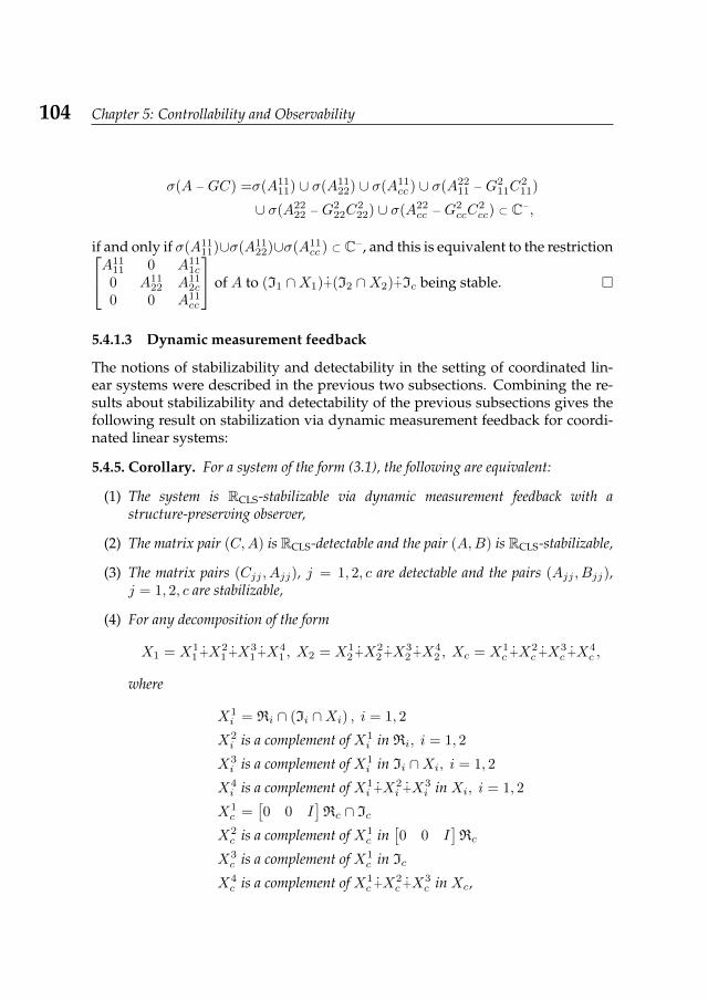
104 Chapter 5: Controllability and Observability
σ(A −GC) =σ(A1111) ∪ σ(A11
22) ∪ σ(A11cc ) ∪ σ(A22
11 −G211C
211)
∪ σ(A2222 −G
222C
222) ∪ σ(A22
cc −G2ccC
2cc) ⊂ C−,
if and only if σ(A1111)∪σ(A11
22)∪σ(A11cc ) ⊂ C−, and this is equivalent to the restrictionA11
11 0 A111c
0 A1122 A11
2c
0 0 A11cc
of A to (I1 ∩X1)+(I2 ∩X2)+Ic being stable.
5.4.1.3 Dynamic measurement feedback
The notions of stabilizability and detectability in the setting of coordinated lin-ear systems were described in the previous two subsections. Combining the re-sults about stabilizability and detectability of the previous subsections gives thefollowing result on stabilization via dynamic measurement feedback for coordi-nated linear systems:
5.4.5. Corollary. For a system of the form (3.1), the following are equivalent:
(1) The system is RCLS-stabilizable via dynamic measurement feedback with astructure-preserving observer,
(2) The matrix pair (C,A) is RCLS-detectable and the pair (A,B) is RCLS-stabilizable,
(3) The matrix pairs (Cjj , Ajj), j = 1, 2, c are detectable and the pairs (Ajj , Bjj),j = 1, 2, c are stabilizable,
(4) For any decomposition of the form
X1 = X11 +X2
1 +X31 +X4
1 , X2 = X12 +X2
2 +X32 +X4
2 , Xc = X1c +X2
c +X3c +X4
c ,
where
X1i = Ri ∩ (Ii ∩Xi) , i = 1, 2
X2i is a complement of X1
i in Ri, i = 1, 2
X3i is a complement of X1
i in Ii ∩Xi, i = 1, 2
X4i is a complement of X1
i +X2i +X3
i in Xi, i = 1, 2
X1c =
[0 0 I
]Rc ∩ Ic
X2c is a complement of X1
c in[0 0 I
]Rc
X3c is a complement of X1
c in Ic
X4c is a complement of X1
c +X2c +X3
c in Xc,
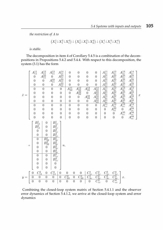
5.4 Systems with inputs and outputs 105
the restriction of A to(X1
1 +X31 +X4
1
)+(X1
2 +X32 +X4
2
)+(X1c +X3
c +X4c
)is stable.
The decomposition in item 4 of Corollary 5.4.5 is a combination of the decom-positions in Propositions 5.4.2 and 5.4.4. With respect to this decomposition, thesystem (3.1) has the form
x =
A1111 A12
11 A1311 A14
11 0 0 0 0 A111c A12
1c A131c A14
1c
0 A2211 0 A24
11 0 0 0 0 A211c A22
1c A231c A24
1c
0 0 A3311 A34
11 0 0 0 0 A311c A32
1c A331c A34
1c
0 0 0 A4411 0 0 0 0 A41
1c A421c A43
1c A441c
0 0 0 0 A1122 A12
22 A1322 A14
22 A112c A12
2c A132c A14
2c
0 0 0 0 0 A2222 0 A24
22 A212c A22
2c A232c A24
2c
0 0 0 0 0 0 A3322 A34
22 A312c A32
2c A332c A34
2c
0 0 0 0 0 0 0 A4422 A41
2c A422c A43
2c A442c
0 0 0 0 0 0 0 0 A11cc A12
cc A13cc A14
cc
0 0 0 0 0 0 0 0 0 A22cc 0 A24
cc
0 0 0 0 0 0 0 0 0 0 A33cc A34
cc
0 0 0 0 0 0 0 0 0 0 0 A44cc
x
+
B111 0 B1
1c
B211 0 B2
1c
0 0 B31c
0 0 B41c
0 B122 B1
2c
0 B222 B2
2c
0 0 B32c
0 0 B42c
0 0 B1cc
0 0 B2cc
0 0 00 0 0
u,
y =
0 C211 0 C4
11 0 0 0 0 C11c C2
1c C31c C4
1c
0 0 0 0 0 C222 0 C4
22 C12c C2
2c C32c C4
2c
0 0 0 0 0 0 0 0 0 C2cc 0 C4
cc
x.Combining the closed-loop system matrix of Section 5.4.1.1 and the observer
error dynamics of Section 5.4.1.2, we arrive at the closed-loop system and errordynamics
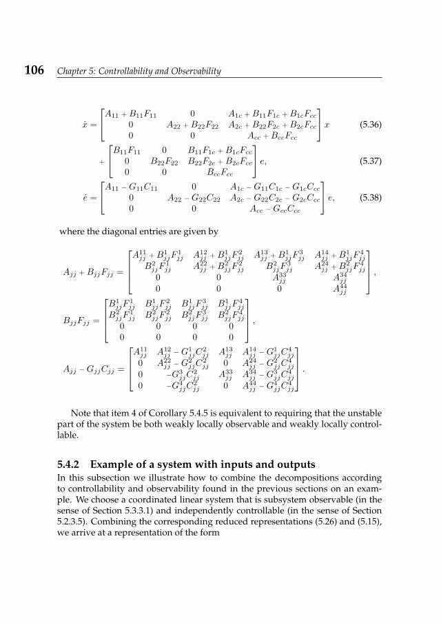
106 Chapter 5: Controllability and Observability
x =
A11 + B11F11 0 A1c + B11F1c + B1cFcc0 A22 + B22F22 A2c + B22F2c + B2cFcc0 0 Acc + BccFcc
x (5.36)
+
B11F11 0 B11F1c + B1cFcc0 B22F22 B22F2c + B2cFcc0 0 BccFcc
e, (5.37)
e =
A11 −G11C11 0 A1c −G11C1c −G1cCcc0 A22 −G22C22 A2c −G22C2c −G2cCcc0 0 Acc −GccCcc
e, (5.38)
where the diagonal entries are given by
Ajj + BjjFjj =
A11jj + B1
jjF1jj A12
jj + B1jjF
2jj A13
jj + B1jjF
3jj A14
jj + B1jjF
4jj
B2jjF
1jj A22
jj + B2jjF
2jj B2
jjF3jj A24
jj + B2jjF
4jj
0 0 A33jj A34
jj
0 0 0 A44jj
,
BjjFjj =
B1jjF
1jj B1
jjF2jj B1
jjF3jj B1
jjF4jj
B2jjF
1jj B2
jjF2jj B2
jjF3jj B2
jjF4jj
0 0 0 00 0 0 0
,
Ajj −GjjCjj =
A11jj A12
jj −G1jjC
2jj A13
jj A14jj −G
1jjC
4jj
0 A22jj −G
2jjC
2jj 0 A24
jj −G2jjC
4jj
0 −G3jjC
2jj A33
jj A34jj −G
3jjC
4jj
0 −G4jjC
2jj 0 A44
jj −G4jjC
4jj
.
Note that item 4 of Corollary 5.4.5 is equivalent to requiring that the unstablepart of the system be both weakly locally observable and weakly locally control-lable.
5.4.2 Example of a system with inputs and outputsIn this subsection we illustrate how to combine the decompositions accordingto controllability and observability found in the previous sections on an exam-ple. We choose a coordinated linear system that is subsystem observable (in thesense of Section 5.3.3.1) and independently controllable (in the sense of Section5.2.3.5). Combining the corresponding reduced representations (5.26) and (5.15),we arrive at a representation of the form
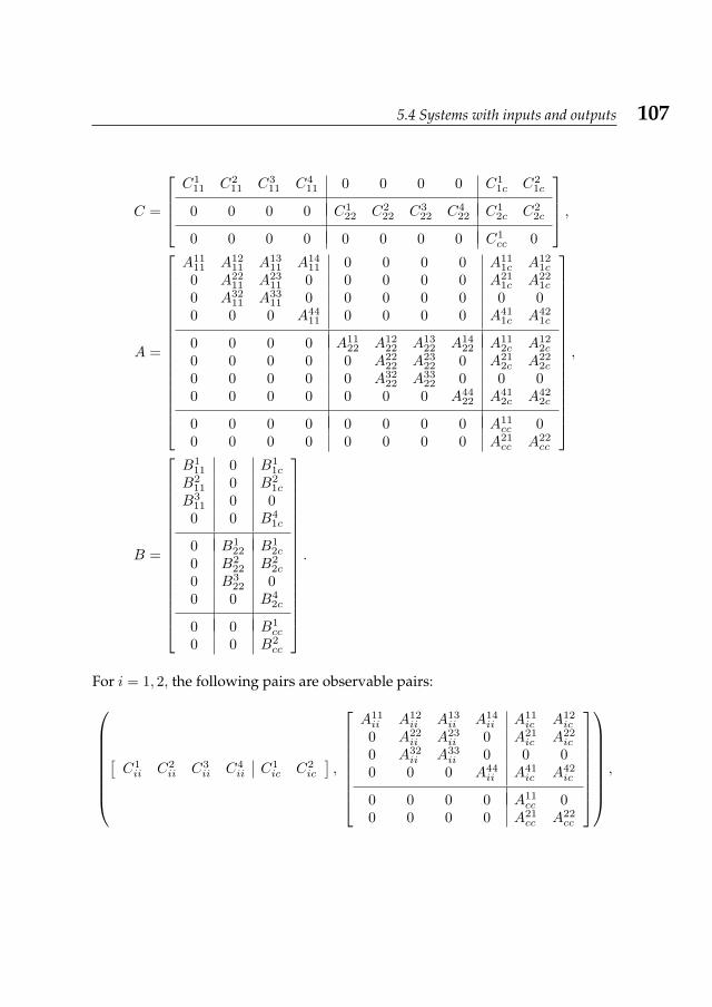
5.4 Systems with inputs and outputs 107
C =
C1
11 C211 C3
11 C411 0 0 0 0 C1
1c C21c
0 0 0 0 C122 C2
22 C322 C4
22 C12c C2
2c
0 0 0 0 0 0 0 0 C1cc 0
,
A =
A1111 A12
11 A1311 A14
11 0 0 0 0 A111c A12
1c
0 A2211 A23
11 0 0 0 0 0 A211c A22
1c
0 A3211 A33
11 0 0 0 0 0 0 00 0 0 A44
11 0 0 0 0 A411c A42
1c
0 0 0 0 A1122 A12
22 A1322 A14
22 A112c A12
2c
0 0 0 0 0 A2222 A23
22 0 A212c A22
2c
0 0 0 0 0 A3222 A33
22 0 0 00 0 0 0 0 0 0 A44
22 A412c A42
2c
0 0 0 0 0 0 0 0 A11cc 0
0 0 0 0 0 0 0 0 A21cc A22
cc
,
B =
B111 0 B1
1c
B211 0 B2
1c
B311 0 00 0 B4
1c
0 B122 B1
2c
0 B222 B2
2c
0 B322 0
0 0 B42c
0 0 B1cc
0 0 B2cc
.
For i = 1, 2, the following pairs are observable pairs:[C1ii C2
ii C3ii C4
ii C1ic C2
ic
],
A11ii A12
ii A13ii A14
ii A11ic A12
ic
0 A22ii A23
ii 0 A21ic A22
ic
0 A32ii A33
ii 0 0 00 0 0 A44
ii A41ic A42
ic
0 0 0 0 A11cc 0
0 0 0 0 A21cc A22
cc
,
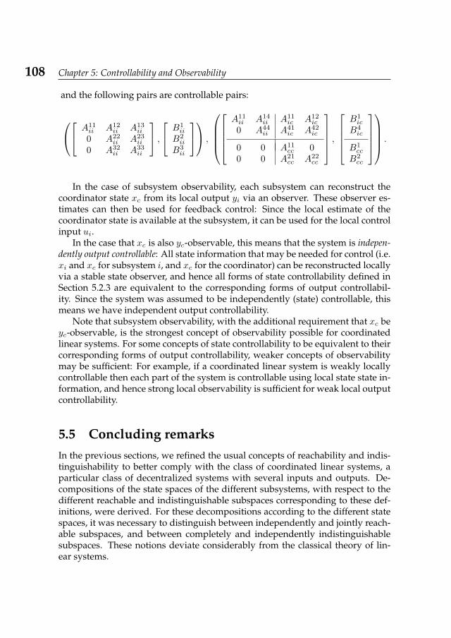
108 Chapter 5: Controllability and Observability
and the following pairs are controllable pairs:
A11ii A12
ii A13ii
0 A22ii A23
ii
0 A32ii A33
ii
, B1
ii
B2ii
B3ii
,
A11ii A14
ii A11ic A12
ic
0 A44ii A41
ic A42ic
0 0 A11cc 0
0 0 A21cc A22
cc
,B1ic
B4ic
B1cc
B2cc
.
In the case of subsystem observability, each subsystem can reconstruct thecoordinator state xc from its local output yi via an observer. These observer es-timates can then be used for feedback control: Since the local estimate of thecoordinator state is available at the subsystem, it can be used for the local controlinput ui.
In the case that xc is also yc-observable, this means that the system is indepen-dently output controllable: All state information that may be needed for control (i.e.xi and xc for subsystem i, and xc for the coordinator) can be reconstructed locallyvia a stable state observer, and hence all forms of state controllability defined inSection 5.2.3 are equivalent to the corresponding forms of output controllabil-ity. Since the system was assumed to be independently (state) controllable, thismeans we have independent output controllability.
Note that subsystem observability, with the additional requirement that xc beyc-observable, is the strongest concept of observability possible for coordinatedlinear systems. For some concepts of state controllability to be equivalent to theircorresponding forms of output controllability, weaker concepts of observabilitymay be sufficient: For example, if a coordinated linear system is weakly locallycontrollable then each part of the system is controllable using local state state in-formation, and hence strong local observability is sufficient for weak local outputcontrollability.
5.5 Concluding remarksIn the previous sections, we refined the usual concepts of reachability and indis-tinguishability to better comply with the class of coordinated linear systems, aparticular class of decentralized systems with several inputs and outputs. De-compositions of the state spaces of the different subsystems, with respect to thedifferent reachable and indistinguishable subspaces corresponding to these def-initions, were derived. For these decompositions according to the different statespaces, it was necessary to distinguish between independently and jointly reach-able subspaces, and between completely and independently indistinguishablesubspaces. These notions deviate considerably from the classical theory of lin-ear systems.
5.5 Concluding remarks 109
While a generalization of our definitions of reachability and indistinguishabil-ity to other classes of decentralized systems is straightforward, the correspondingdecompositions quickly become infeasible if the underlying information struc-ture is less restrictive. However, the distinction between independent and jointreachability, and between complete and independent indistinguishability, may berelevant for other classes of decentralized linear systems as well.
When defining the concepts of controllability and observability, we again hadto deviate from the classical definitions for unstructured systems: These proper-ties of linear systems in their usual sense are of little practical use for coordinatedlinear systems, and cannot be verified in a decentralized manner. Instead, weintroduced the slightly stronger concepts of independent controllability and ob-servability, related to the notion of independence needed for the decompositions.In contrast to the case of unstructured linear systems, these new concepts did notsuffice for pole placement and state reconstruction; for this, we needed the con-cepts of weak local controllability and observability, which easily carry over toother linear systems with a top-to-bottom information structure.
For stabilizability and detectability, and consequently for stabilization via dy-namic measurement feedback, we again needed the concepts of weak local con-trollability and observability, rather than the usual concepts or their independentcounterparts. This is due to the necessary restriction of admissible feedbacks andobservers to the ones complying with the underlying information structure. Thiseffect of restricting the admissible feedbacks will also play an important role inlinear-quadratic optimal control for coordinated linear systems, as described inthe following chapter.
110 Chapter 5: Controllability and Observability
LQ Optimal Control 6In this chapter, we extend the classical LQ optimal control problem for monolithiclinear systems, the formulation and solution of which was summarized in Section2.4, to coordinated linear systems.
This chapter is submitted as [22], and the corresponding numerical algorithmand computations can be found in [70]. Based on the results derived here, therelated case of LQ control for coordinated Gaussian systems was worked out in[41].
6.1 IntroductionThe classical LQ (linear-quadratic) optimal control problem was first formulatedand solved in [20]1, and has played a central role in system theory ever since –on the one hand because of its wide applicability, and on the other hand becauseof the computational and conceptual simplicity of its solution. Unfortunately, theoptimal control feedback u(·) = Gx(·), obtained by solving the Riccati equation(2.10) for a coordinated linear system, does in general not respect the underlyinginformation structure. Hence, in order to apply the classical theory to the case ofcoordinated linear systems, we need to add the constraint that the state feedbackshould be an element of RCLS.
The main results of this chapter state that
• the LQ problem for coordinated linear systems separates into independentlocal problems for each subsystem and a more complex problem at the co-ordinator level,
• due to this separation property, the LQ problem for any hierarchical systemwhose information structure forms a directed tree can be separated intosubproblems and approached in a bottom-to-top manner,
• and in contrast to the unstructured case, the optimal feedback matrix doesdepend on the initial state.
For notational reasons, and using the separability of the problem describedabove, we first restrict attention to the special case of leader-follower systems, i.e.hierarchical systems with two layers and only one subsystem at each layer, andthen extend these results to coordinated linear systems, and more general hier-archical systems. The results are reformulated into control synthesis procedures,and the theory is illustrated in an example involving vehicle formations.
1According to scholar.google.com, this will be roughly the 1100th time that [20] is cited.
112 Chapter 6: LQ Optimal Control
6.2 LQ control for leader-follower systemsIn this section we consider LQ optimal control for leader-follower systems. Exten-sions of the results of this section to coordinated linear systems and hierarchicalsystems are discussed in Section 6.3.
For the purposes of this section, we denote the set of block upper-triangularmatrices by
R4 =
[Mss Msc
0 Mcc
], Mij ∈ Rmi×nj , i, j = s, c
.
6.2.1 Problem formulationThe control problem considered in this section is defined for two different sets ofadmissible control laws:
6.2.1. Problem. We consider leader-follower systems, of the form[xsxc
](t) =
[Ass Asc0 Acc
] [xsxc
](t) +
[Bss Bsc0 Bcc
] [usuc
](t),
[xsxc
](0) =
[x0,s
x0,c
](6.1)
and quadratic infinite-horizon undiscounted cost functions, of the form
J
(x0,
[us(·)uc(·)
])=
∫ ∞0
[xsxc
]T [Qss 00 Qcc
] [xsxc
]+
[usuc
] [Rss 00 Rcc
] [usuc
]dt, (6.2)
where Qss ≥ 0, Qcc ≥ 0, Rss > 0, and Rcc > 0.We want to minimize the cost function over the following sets of admissible
control laws:2
U4lin=
[Fss Fsc0 Fcc
]x(t)
∣∣∣∣A + BF is stable, F may depend on x0
,
U4=
[us(t, xs, xc)uc(t, xs,0, xc)
]∣∣∣∣us and uc are stabilizing and piecewise continuous in t,us and uc depend causally on xs and xc
.
The control problems considered in this section are hence given by
minu(·)∈U4
J (x0, u(·)) , (6.3)
minu(·)=Fx(·)∈U4lin
J(x0, Fx(·)). (6.4)
2In this context, we call a control law u(·) stabilizing if applying the control law u(·) leads to anexponentially decaying system state for t→∞.
6.2 LQ control for leader-follower systems 113
The set U4 contains all (linear or nonlinear) admissible control laws whichrespect the underlying information structure of the system. The set U4lin ⊂ U4 re-stricts the admissible control laws to structure-preserving linear state feedbacks.
Note that in both sets of admissible control laws, the initial state x0 is assumedto be globally known: The coordinator system may use the subsystem initial statex0,s, even though this does not respect the information structure. From the theorydeveloped in this section, it will become clear that this additional knowledge hasa large impact on the optimal coordinator feedback, and on the overall cost.
6.2.2 Optimal control over U4
The most straightforward option for extending the centralized solution given inSection 2.4 to the more restrictive control problem (6.3) is to include a copy ofthe subsystem in the coordinator. Since the state trajectory of a deterministiclinear system can be reconstructed from the initial state and the closed-loop statetransition matrix, the coordinator only needs to know xs,0 and the matrix A+BGin order to deduce the state xs(t) at each time t. The coordinator can then applythe optimal feedback of the centralized case, using its local copy of xs(t). With
this construction, and writingG =
[Gss GscGcs Gcc
], we get the coordinator control law
uc(·, xs,0, xc(·)) = Gcsz(·) + Gccxc(·),
with z(·) given by the internal reconstruction
z = (Ass + BssGss)z + BssGscxc, z(0) = xs,0
of xs(·). This control law for the coordinator does not depend on xs(t) (but onlyon its local reconstruction), and hence respects the information structure imposedon the system. Together with the subsystem control law
us(·, xs(·), xc(·)) = Gssxs(·) + Gscxc(·),
we have that[usuc
]∈ U4. Since the resulting closed-loop system is equivalent to
the system x = (A +BG)x, this control law achieves the same optimal cost as thecentralized control law Gx(·):
minu(·)∈U4
J(x0, u(·)) = J(x0, Gx(·)).
114 Chapter 6: LQ Optimal Control
From this it also follows that the control law[us(·)uc(·)
]constructed here is stabilizing
if and only if Gx(·) is stabilizing, and hence the conditions for well-definednessof the control problem over U4 are the same as in the centralized case, i.e. that(A,B) be a stabilizable pair, and (Q,A) be a detectable pair.
In [56, 61] it is shown that the construction above corresponds to the controllaw obtained from solving the decentralized control problem in an input-outputframework, and then translating the solution back to its state-space equivalent.
However the control law constructed above, based on reconstructing the sub-system state at the coordinator level, has several disadvantages:
• In a hierarchical system, the subsystem state xs comprises all parts of thesystem which are influenced by the coordinator (see Section 6.3). Hence theapproach used here is not scalable for large hierarchical systems: The sim-ulation of the subsystem at the coordinator level becomes computationallyvery involved.
• Moreover, this approach is not extendable to systems with disturbancesor parameter uncertainties: The actual subsystem state may diverge fromits reconstruction by the coordinator, leading to arbitrarily large costs, andeven to loss of stability. This is because after the initial time, the coordina-tor receives no feedback from the subsystem, and hence cannot adjust itsestimate accordingly.
In Chapter 7, we present one alternative to the control law found in this section,using event-based feedback from the subsystem(s) to the coordinator. In the restof this chapter we present another alternative, using the restriction that the coor-dinator control law uc must be a linear state feedback of the form uc(·) = Fccxc(·).
6.2.3 Optimal control over U4lin
In the following we develop the core results of the chapter – the well-definedness,separability and solution of Problem (6.4).
6.2.3.1 Conditions for well-definedness
In this subsection we introduce the concepts of R4-stabilizability and R4-detectability, and show that these concepts are necessary and sufficient for thewell-definedness of Problem (6.4).
Stabilizability. In Section 5.4.1.1 it was shown that, for the case of coordinatedlinear systems, the usual concept of stabilizability needs to be restricted to theexistence of a stabilizing structure-preserving feedback. We simplify Definition
6.2 LQ control for leader-follower systems 115
5.4.1 of RCLS-stabilizability (for coordinated linear systems) to R4-stabilizability(for leader-follower systems):
6.2.2. Definition. We call a system of the form (6.1) R4-stabilizable if there existsa feedback matrix
F =
[Fss Fsc0 Fcc
]∈ R4
such that the closed-loop system matrix A + BF is stable.
The following proposition is simplified from Proposition 5.4.2:
6.2.3. Proposition. A system of the form (6.1) is R4-stabilizable if and only if the matrixpairs (Ass, Bss) and (Acc, Bcc) are stabilizable pairs.
Detectability. Similarly, we modify Definition 5.4.3 of RCLS-detectability, whichaccounts for the restriction that possible observers must respect the underlyinginformation structure. For this, we first need to define leader-follower systemswith outputs: [
xsxc
]=
[Ass Asc0 Acc
] [xsxc
]+
[Bss Bsc0 Bcc
] [usuc
],[
ysyc
]=
[Css Csc0 Ccc
] [xsxc
].
(6.5)
The role of the output matrix C will later be replaced by the cost matrix Q.
6.2.4. Definition. We call a system of the form (6.5) R4-detectable if there existsan observer gain
K =
[Kss Ksc
0 Kcc
]∈ R4
such that the observer-error matrix A −KC is stable.
The following proposition is simplified from Proposition 5.4.4:
6.2.5. Proposition. A system of the form (6.5) is R4-detectable if and only if the matrixpairs (Css, Ass) and (Ccc, Acc) are detectable pairs.
Conditions for well-definedness. Now we can give a sufficient condition forwell-definedness of Problem (6.4), using stabilizability and detectability proper-ties of the corresponding submatrices:
6.2.6. Proposition. If the pairs (Ass, Bss) and (Acc, Bcc) are stabilizable pairs, andif the pairs (Qss, Ass) and (Qcc, Acc) are detectable pairs, then Problem (6.4) is well-defined, i.e. it admits a stabilizing solution, which lies inside U4lin.
116 Chapter 6: LQ Optimal Control
Proof. Since (Ass, Bss) is a stabilizable pair and (Qss, Ass) is a detectable pair, theequation
XssBssR−1ssBssXss −A
TssXss −XssAss −Qss = 0
has a stabilizing solution Xss. Similarly, the equation
XccBccR−1ccBccXcc −A
TccXcc −XccAcc −Qcc = 0
has a stabilizing solution Xcc. Consider the feedback F =
[Fss 00 Fcc
], with
Fss = −R−1ssB
TssXss and Fcc = −R−1
ccBTccXcc. To show that F is indeed a stabi-
lizing feedback, we look at the spectrum of the closed-loop system:
σ
([Ass Asc0 Acc
]+
[Bss Bsc0 Bcc
] [Fss 00 Fcc
])= σ
([Ass + BssFss Asc + BscFcc
0 Acc + BccFcc
])= σ (Ass + BssFss) ∪ σ (Acc + BccFcc) ∈ C−.
We conclude that there exists a stabilizing feedback F ∈ U4lin, leading to a finitecost (this follows directly from stability of the closed-loop system).
In order to show that the infimum over U4lin is indeed a minimum, we notethat on the boundary of the set of all stabilizing feedback matrices, the closed-loop system has at least one eigenvalue on the imaginary axis, and hence onepart of the closed-loop system is not exponentially stable. If the initial conditionfor this part is non-zero, then the state will never vanish, and by detectability ofthe system, the corresponding cost will be infinite. We conclude that the infimumover U4lin is attained at a point in the interior of U4lin, and hence it is a minimum.
6.2.3.2 Conditionally-optimal solution, given Fcc
For the purpose of this subsection, suppose that the coordinator feedback Fcc isfixed. Replacing the coordinator input uc with Fccxc, we then have the system[
xsxc
](t) =
[Ass Asc + BscFcc0 Acc + BccFcc
] [xsxc
](t) +
[Bss0
]us(t),
[xsxc
](0) =
[x0,s
x0,c
]. (6.6)
The cost function becomes
JFcc(x0, us(·)) =
∫ ∞0
[xsxc
]T [Qss 00 Qcc + FTccRccFcc
] [xsxc
]+ usRssus dt.
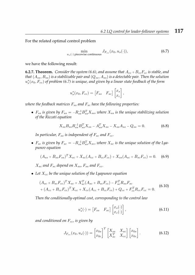
6.2 LQ control for leader-follower systems 117
For the related optimal control problem
minus(·) piecewise continuous
JFcc(x0, us(·)), (6.7)
we have the following result:
6.2.7. Theorem. Consider the system (6.6), and assume that Acc +BccFcc is stable, andthat (Ass, Bss) is a stabilizable pair and (Qss, Ass) is a detectable pair. Then the solutionu∗s(x0, Fcc) of problem (6.7) is unique, and given by a linear state feedback of the form
u∗s(x0, Fcc) =[Fss Fsc
] [xsxc
],
where the feedback matrices Fss and Fsc have the following properties:
• Fss is given by Fss = −R−1ssB
TssXss, where Xss is the unique stabilizing solution
of the Riccati equation
XssBssR−1ssB
TssXss −A
TssXss −XssAss −Qss = 0. (6.8)
In particular, Fss is independent of Fsc and Fcc.
• Fsc is given by Fsc = −R−1ssB
TssXsc, where Xsc is the unique solution of the Lya-
punov equation
(Ass + BssFss)TXsc + Xsc(Acc + BccFcc) + Xss(Asc + BscFcc) = 0. (6.9)
Xsc and Fsc depend on Xss, Fss and Fcc.
• Let Xcc be the unique solution of the Lyapunov equation
(Asc + BscFcc)TXsc + XT
sc(Asc + BscFcc) − FTscRssFsc
+ (Acc + BccFcc)TXcc + Xcc(Acc + BccFcc) + Qcc + FTccRccFcc = 0.
(6.10)
Then the conditionally-optimal cost, corresponding to the control law
u∗s(·) =[Fss Fsc
] [xs(·)xc(·)
], (6.11)
and conditioned on Fcc, is given by
JFcc(x0, us(·)) =
[x0s
x0c
]T [Xss Xsc
XTsc Xcc
] [x0s
x0c
]. (6.12)
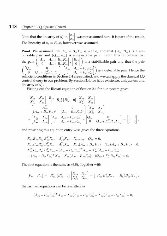
118 Chapter 6: LQ Optimal Control
Note that the linearity of u∗s in[xsxc
]was not assumed here; it is part of the result.
The linearity of uc = Fccxc however was assumed.
Proof. We assumed that Acc + BccFcc is stable, and that (Ass, Bss) is a sta-bilizable pair and (Qss, Ass) is a detectable pair. From this it follows that
the pair([Ass Asc + BscFcc0 Acc + BccFcc
],
[Bss0
])is a stabilizable pair and that the pair([
Qss 00 Qcc + FTccRccFcc
],
[Ass Asc + BscFcc0 Acc + BccFcc
])is a detectable pair. Hence the
sufficient conditions in Section 2.4 are satisfied, and we can apply the classical LQcontrol theory to our problem. By Section 2.4, we have existence, uniqueness andlinearity of u∗s .
Writing out the Riccati equation of Section 2.4 for our system gives[Xss Xsc
XTsc Xcc
] [Bss0
]R−1ss
[BTss 0
] [Xss Xsc
XTsc Xcc
]−
[ATss 0
(Asc + BscFcc)T (Acc + BccFcc)
T
] [Xss Xsc
XTsc Xcc
]−
[Xss Xsc
XTsc Xcc
] [Ass Asc + BscFcc0 Acc + BccFcc
]−
[Qss 00 Qcc + FTccRccFcc
]=
[0 00 0
],
and rewriting this equation entry-wise gives the three equations
XssBssR−1ssB
TssXss −A
TssXss −XssAss −Qss = 0,
XssBssR−1ssB
TssXsc −A
TssXsc −Xss(Asc + BscFcc) −Xsc(Acc + BccFcc) = 0,
XTscBssR
−1ssB
TssXsc − (Asc + BscFcc)
TXsc −XTsc(Asc + BscFcc)
− (Acc + BccFcc)TXcc −Xcc(Acc + BccFcc) − (Qcc + FTccRccFcc) = 0.
The first equation is the same as (6.8). Together with
[Fss Fsc
]= −R−1
ss
[BTss 0
] [Xss Xsc
XTsc Xcc
]=[−R−1
ssBTssXss −R−1
ssBTssXsc
],
the last two equations can be rewritten as
(Ass + BssFss)TXsc + Xsc(Acc + BccFcc) + Xss(Asc + BscFcc) = 0,
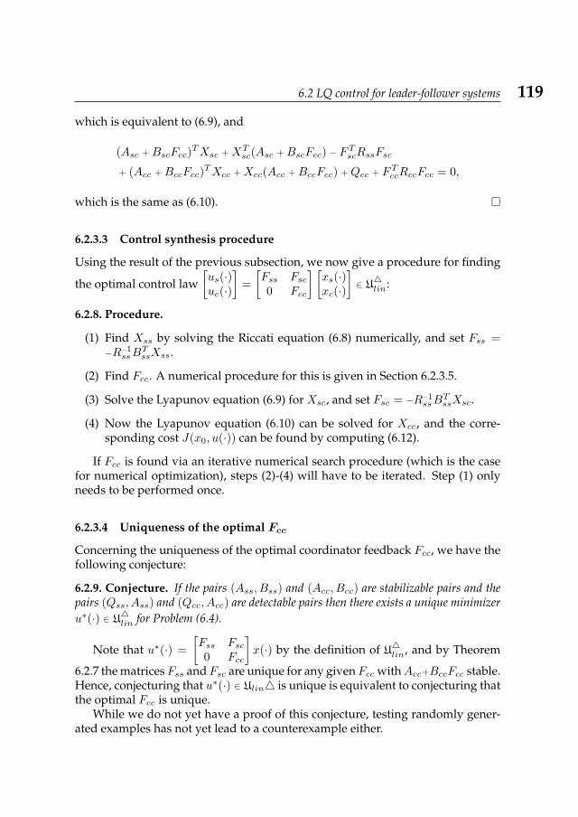
6.2 LQ control for leader-follower systems 119
which is equivalent to (6.9), and
(Asc + BscFcc)TXsc + XT
sc(Asc + BscFcc) − FTscRssFsc
+ (Acc + BccFcc)TXcc + Xcc(Acc + BccFcc) + Qcc + FTccRccFcc = 0,
which is the same as (6.10).
6.2.3.3 Control synthesis procedure
Using the result of the previous subsection, we now give a procedure for finding
the optimal control law[us(·)uc(·)
]=
[Fss Fsc0 Fcc
] [xs(·)xc(·)
]∈ U4lin:
6.2.8. Procedure.
(1) Find Xss by solving the Riccati equation (6.8) numerically, and set Fss =−R−1
ssBTssXss.
(2) Find Fcc. A numerical procedure for this is given in Section 6.2.3.5.
(3) Solve the Lyapunov equation (6.9) for Xsc, and set Fsc = −R−1ssB
TssXsc.
(4) Now the Lyapunov equation (6.10) can be solved for Xcc, and the corre-sponding cost J(x0, u(·)) can be found by computing (6.12).
If Fcc is found via an iterative numerical search procedure (which is the casefor numerical optimization), steps (2)-(4) will have to be iterated. Step (1) onlyneeds to be performed once.
6.2.3.4 Uniqueness of the optimal Fcc
Concerning the uniqueness of the optimal coordinator feedback Fcc, we have thefollowing conjecture:
6.2.9. Conjecture. If the pairs (Ass, Bss) and (Acc, Bcc) are stabilizable pairs and thepairs (Qss, Ass) and (Qcc, Acc) are detectable pairs then there exists a unique minimizeru∗(·) ∈ U4lin for Problem (6.4).
Note that u∗(·) =
[Fss Fsc0 Fcc
]x(·) by the definition of U4lin, and by Theorem
6.2.7 the matricesFss andFsc are unique for any givenFcc withAcc+BccFcc stable.Hence, conjecturing that u∗(·) ∈ Ulin4 is unique is equivalent to conjecturing thatthe optimal Fcc is unique.
While we do not yet have a proof of this conjecture, testing randomly gener-ated examples has not yet lead to a counterexample either.
120 Chapter 6: LQ Optimal Control
6.2.3.5 Finding Fcc numerically
So far we have not found an analytical solution for the problem of finding theoptimal Fcc.
Setting F indcc = −R−1ccB
TccYcc, where Ycc is the unique stabilizing solution of the
local Riccati equation
YccBccR−1ccB
TccYcc −A
TccYcc − YccAcc −Qcc = 0,
is always an admissible option (see the proof of Proposition 6.2.6), although usu-ally not the optimal one. It can however serve as a good initial value for numeri-cal optimization procedures.
One approach to finding the optimal solution numerically is to use the Matlabroutine fmincon to minimize the cost over all possible Fcc, with the constraintthat Fcc must be stabilizing. This approach is implemented in [70] (for coordi-nated linear systems) as follows:
• The feedback F indcc is used as starting value for fmincon,
• The local feedback Fss is computed from equation (6.8),
• At each step of the optimization procedure, the cost corresponding to thecurrent value of Fcc is computed using equations (6.9)-(6.12) if Acc +BccFccis stable, and set to∞ otherwise.
Testing this algorithm for randomly generated examples, we found that it alwaysconverges to an admissible solution, and that the cost difference compared tothe centralized feedback is in general very small, and often even negligible. Thecomputation time scales exponentially with the problem size.
The set of all stabilizing Fcc is not a convex set with respect to its element-wiseparametrizationFcc =
f1,1 · · · f1,nc
.... . .
...fmc,1 · · · fmc,nc
, f i,j ∈ R, σ (Acc + BccFcc) ⊂ C−
.
Hence there is no guarantee that the algorithm described above will perform wellin all situations. It is, however, a connected set, and alternative parameterizationswould lead to convexity. Whether a parametrization exists which would leadto convexity of both the set of stabilizing feedbacks and the objective functionrestricted to this set, is an open question.
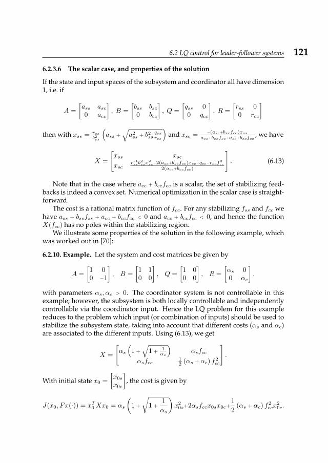
6.2 LQ control for leader-follower systems 121
6.2.3.6 The scalar case, and properties of the solution
If the state and input spaces of the subsystem and coordinator all have dimension1, i.e. if
A =
[ass asc0 acc
], B =
[bss bsc0 bcc
], Q =
[qss 00 qcc
], R =
[rss 00 rcc
]
then with xss = rssb2ss
(ass +
√a2ss + b2ss
qssrss
)and xsc = −(asc+bscfcc)xss
ass+bssfss+acc+bccfcc, we have
X =
[xss xsc
xscr−1ssb
2ssx
2sc−2(asc+bscfcc)xsc−qcc−rccf
2cc
2(acc+bccfcc)
]. (6.13)
Note that in the case where acc + bccfcc is a scalar, the set of stabilizing feed-backs is indeed a convex set. Numerical optimization in the scalar case is straight-forward.
The cost is a rational matrix function of fcc. For any stabilizing fss and fcc wehave ass + bssfss + acc + bccfcc < 0 and acc + bccfcc < 0, and hence the functionX(fcc) has no poles within the stabilizing region.
We illustrate some properties of the solution in the following example, whichwas worked out in [70]:
6.2.10. Example. Let the system and cost matrices be given by
A =
[1 00 −1
], B =
[1 10 0
], Q =
[1 00 0
], R =
[αs 00 αc
],
with parameters αs, αc > 0. The coordinator system is not controllable in thisexample; however, the subsystem is both locally controllable and independentlycontrollable via the coordinator input. Hence the LQ problem for this examplereduces to the problem which input (or combination of inputs) should be used tostabilize the subsystem state, taking into account that different costs (αs and αc)are associated to the different inputs. Using (6.13), we get
X =
[αs
(1 +
√1 + 1
αs
)αsfcc
αsfcc12 (αs + αc) f
2cc
].
With initial state x0 =
[x0s
x0c
], the cost is given by
J(x0, Fx(·)) = xT0 Xx0 = αs
(1 +
√1 +
1
αs
)x2
0s+2αsfccx0sx0c+1
2(αs + αc) f
2ccx
20c.
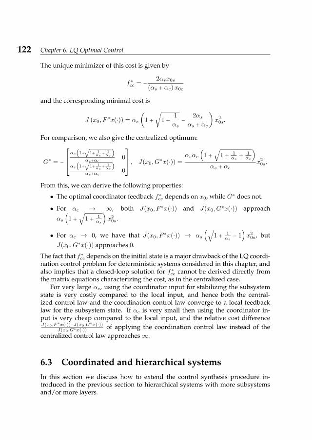
122 Chapter 6: LQ Optimal Control
The unique minimizer of this cost is given by
f∗cc = −2αsx0s
(αs + αc)x0c
and the corresponding minimal cost is
J (x0, F∗x(·)) = αs
(1 +
√1 +
1
αs−
2αsαs + αc
)x2
0s.
For comparison, we also give the centralized optimum:
G∗ = −
αc(
1+
√1+ 1
αs+ 1αc
)αs+αc
0
αs(
1+
√1+ 1
αs+ 1αc
)αs+αc
0
, J(x0, G∗x(·)) =
αsαc
(1 +
√1 + 1
αs+ 1αc
)αs + αc
x20s.
From this, we can derive the following properties:
• The optimal coordinator feedback f∗cc depends on x0, while G∗ does not.
• For αc → ∞, both J(x0, F∗x(·)) and J(x0, G
∗x(·)) approach
αs
(1 +
√1 + 1
αs
)x2
0s.
• For αc → 0, we have that J(x0, F∗x(·)) → αs
(√1 + 1
αs− 1)x2
0s, butJ(x0, G
∗x(·)) approaches 0.
The fact that f∗cc depends on the initial state is a major drawback of the LQ coordi-nation control problem for deterministic systems considered in this chapter, andalso implies that a closed-loop solution for f∗cc cannot be derived directly fromthe matrix equations characterizing the cost, as in the centralized case.
For very large αc, using the coordinator input for stabilizing the subsystemstate is very costly compared to the local input, and hence both the central-ized control law and the coordination control law converge to a local feedbacklaw for the subsystem state. If αc is very small then using the coordinator in-put is very cheap compared to the local input, and the relative cost differenceJ(x0,F
∗x(·))−J(x0,G∗x(·))
J(x0,G∗x(·)) of applying the coordination control law instead of thecentralized control law approaches∞.
6.3 Coordinated and hierarchical systemsIn this section we discuss how to extend the control synthesis procedure in-troduced in the previous section to hierarchical systems with more subsystemsand/or more layers.
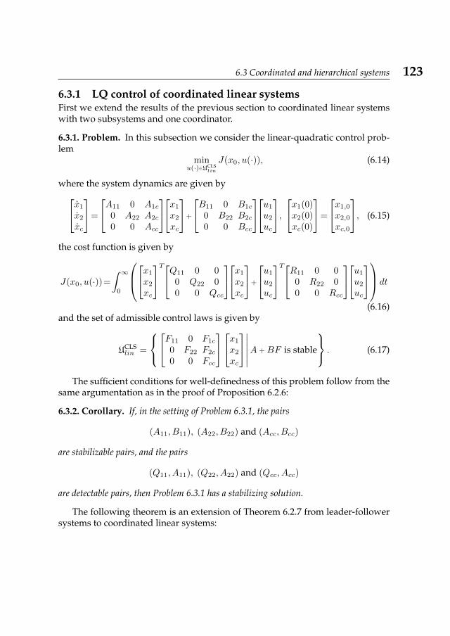
6.3 Coordinated and hierarchical systems 123
6.3.1 LQ control of coordinated linear systemsFirst we extend the results of the previous section to coordinated linear systemswith two subsystems and one coordinator.
6.3.1. Problem. In this subsection we consider the linear-quadratic control prob-lem
minu(·)∈UCLS
lin
J(x0, u(·)), (6.14)
where the system dynamics are given byx1
x2
xc
=
A11 0 A1c
0 A22 A2c
0 0 Acc
x1
x2
xc
+
B11 0 B1c
0 B22 B2c
0 0 Bcc
u1
u2
uc
,x1(0)x2(0)xc(0)
=
x1,0
x2,0
xc,0
, (6.15)
the cost function is given by
J(x0, u(·))=
∫ ∞0
x1
x2
xc
TQ11 0 00 Q22 00 0 Qcc
x1
x2
xc
+
u1
u2
uc
TR11 0 00 R22 00 0 Rcc
u1
u2
uc
dt
(6.16)and the set of admissible control laws is given by
UCLSlin =
F11 0 F1c
0 F22 F2c
0 0 Fcc
x1
x2
xc
∣∣∣∣∣∣A + BF is stable
. (6.17)
The sufficient conditions for well-definedness of this problem follow from thesame argumentation as in the proof of Proposition 6.2.6:
6.3.2. Corollary. If, in the setting of Problem 6.3.1, the pairs
(A11, B11), (A22, B22) and (Acc, Bcc)
are stabilizable pairs, and the pairs
(Q11, A11), (Q22, A22) and (Qcc, Acc)
are detectable pairs, then Problem 6.3.1 has a stabilizing solution.
The following theorem is an extension of Theorem 6.2.7 from leader-followersystems to coordinated linear systems:
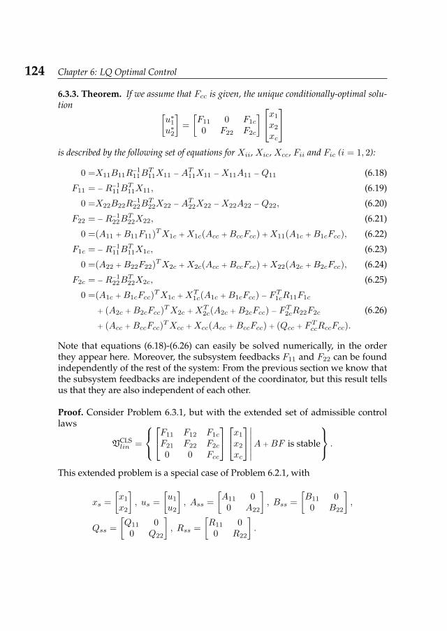
124 Chapter 6: LQ Optimal Control
6.3.3. Theorem. If we assume that Fcc is given, the unique conditionally-optimal solu-tion [
u∗1u∗2
]=
[F11 0 F1c
0 F22 F2c
]x1
x2
xc
is described by the following set of equations for Xii, Xic, Xcc, Fii and Fic (i = 1, 2):
0 =X11B11R−111B
T11X11 −A
T11X11 −X11A11 −Q11 (6.18)
F11 = −R−111B
T11X11, (6.19)
0 =X22B22R−122B
T22X22 −A
T22X22 −X22A22 −Q22, (6.20)
F22 = −R−122B
T22X22, (6.21)
0 =(A11 + B11F11)TX1c + X1c(Acc + BccFcc) + X11(A1c + B1cFcc), (6.22)
F1c = −R−111B
T11X1c, (6.23)
0 =(A22 + B22F22)TX2c + X2c(Acc + BccFcc) + X22(A2c + B2cFcc), (6.24)
F2c = −R−122B
T22X2c, (6.25)
0 =(A1c + B1cFcc)TX1c + XT
1c(A1c + B1cFcc) − FT1cR11F1c
+ (A2c + B2cFcc)TX2c + XT
2c(A2c + B2cFcc) − FT2cR22F2c
+ (Acc + BccFcc)TXcc + Xcc(Acc + BccFcc) + (Qcc + FTccRccFcc).
(6.26)
Note that equations (6.18)-(6.26) can easily be solved numerically, in the orderthey appear here. Moreover, the subsystem feedbacks F11 and F22 can be foundindependently of the rest of the system: From the previous section we know thatthe subsystem feedbacks are independent of the coordinator, but this result tellsus that they are also independent of each other.
Proof. Consider Problem 6.3.1, but with the extended set of admissible controllaws
VCLSlin =
F11 F12 F1c
F21 F22 F2c
0 0 Fcc
x1
x2
xc
∣∣∣∣∣∣A + BF is stable
.
This extended problem is a special case of Problem 6.2.1, with
xs =
[x1
x2
], us =
[u1
u2
], Ass =
[A11 00 A22
], Bss =
[B11 00 B22
],
Qss =
[Q11 0
0 Q22
], Rss =
[R11 00 R22
].
6.3 Coordinated and hierarchical systems 125
Thus, fixing Fcc, we can use Theorem 6.2.7 to find the conditionally-optimal con-trol law for the extended problem. Rewriting equation (6.8) for this case, with
Xss =
[X11 X12
XT12 X22
], we get
[X11 X12
XT12 X22
] [B11 00 B22
] [R−1
11 00 R−1
22
] [BT11 00 BT22
] [X11 X12
XT12 X22
]−
[AT11 00 AT22
] [X11 X12
XT12 X22
]−
[X11 X12
XT12 X22
] [A11 00 A22
]−
[Q11 0
0 Q22
]= 0.
The matrix[X11 0
0 X22
], with X11 and X22 the stabilizing solutions of (6.18)
and (6.20), respectively, is a solution of this Riccati equation. Moreover,
the corresponding feedback Fss =
[−R−1
11BT11X11 0
0 −R−122B
T22X22
]is stabiliz-
ing: The choice of X11 and X22 ensures that the closed-loop subsystem matrix[A11 −B11R
−111B
T11X11 0
0 A22 −B22R−122B
T22X22
]is stable. But the stabilizing solu-
tion of a Riccati equation is unique, and hence[X11 0
0 X22
]is the only stabilizing
solution. From this it follows that
Fss = −R−1ssB
TssXss = −
[R−1
11 00 R−1
22
] [BT11 00 BT22
] [X11 0
0 X22
]is automatically block-diagonal. This means that the conditionally-optimal solu-tion of Problem 6.3.1 over the extended set VCLS
lin is an element of UCLSlin , and since
UCLSlin ⊆ VCLS
lin , it is also the conditionally-optimal solution over UCLSlin .
Equation (6.9) splits into equations (6.22) and (6.24), and equation (6.10) re-duces to (6.26).
In light of Theorem 6.3.3, we can now extend Procedure 6.2.8 to a controlsynthesis procedure for coordinated linear systems:
6.3.4. Procedure.
(1) Find X11 and X22 by solving the Riccati equations (6.18) and (6.20) numer-ically, and set F11 = −R−1
11BT11X11 and F22 = −R−1
22BT22X22.
(2) Combine the two subsystems to one system: Set
Ass =
[A11 00 A22
], Bss =
[B11 00 B22
], Qss =
[Q11 0
0 Q22
], Rss =
[R11 00 R22
],
126 Chapter 6: LQ Optimal Control
and fix Fss =
[F11 00 F22
].
(3) Use steps (2)-(4) of Procedure 6.2.8 to find the optimal coordination controlfeedback for the problem.
6.3.2 Extension to hierarchical systemsIn this subsection we discuss how to extend the results and procedures above tomore general hierarchical systems, with several layers and/or more subsystemsat each layer.
6.3.5. Problem. Let a hierarchical linear system, i.e. a distributed linear systemwith its underlying information structure given by a directed tree, be given. Wewill assume that the system is both locally stabilizable and locally detectable, i.e.for each subsystem j in the hierarchy we assume that (Ajj , Bjj) is a stabilizablepair and (Qjj , Ajj) is a detectable pair. We consider the infinite-horizon LQ con-trol problem with Q and R block-diagonal, and restricting the set of admissiblefeedback matrices to those which respect the system’s information structure.
For hierarchical systems, control is done in a bottom-up manner: First we findlocal feedbacks for the subsystems which do not act as coordinators for any otherpart of the system (i.e. the leaves of the corresponding directed tree), and thenwe find the optimal feedbacks for the coordinating systems, using the results andprocedures of the previous sections.
6.3.6. Procedure.
• Pick a subsystem j, all followers3 of which already have local feedbacksassigned to them (or no followers exist).
• For this subsystem, calculate the solution Xindjj of the local Riccati equation
Xindjj BjjR
−1jjB
TjjX
indjj −ATjjX
indjj −Xind
jj Ajj −Qjj = 0.
• Starting with F indjj = −R−1jjB
TjjX
indjj , find the optimal Fjj numerically: Con-
sider all followers of system j as one subsystem, and find Fjj using thenumerical optimization procedure described in Section 6.2.3.5.
• Set uj = Fjjxj , find
F1j
...Fsjj
from (6.9), and apply the feedbacks Fkjxj to all
followers k of system j.
3By followers, we mean all subsystems which are coordinated by system j.
6.4 Example: Vehicle formations 127
Repeatedly applying the results of the previous sections, and assuming thatthe algorithm of Section 6.2.3.5 indeed converges to the global optimum, we findthat the feedback F found by Procedure 6.3.6 is the optimal linear state feedbackwhich respects the information structure.
6.4 Example: Vehicle formationsIn order to illustrate the control synthesis procedures introduced in this paper, weapply our results to a toy example involving several autonomous vehicles. Thegoal of the vehicles is to maintain a fixed formation while tracking a referencesignal. Even though all subsystems have the same internal dynamics, the optimalcontrol feedback for each vehicle will be different, depending on the number andformation of its followers.
Each vehicle Vj is modeled by a very simple linear system, with its positionpj ∈ R3 and velocity vj ∈ R3 as state variables, and its acceleration aj ∈ R3 ascontrol input. For vehicle Vj , this system is given by[
pjvj
]=
[0 I0 0
] [pjvj
]+
[0I
]aj ,
[pjvj
](0) =
[pj,0vj,0
]. (6.27)
For each vehicle, we moreover have a reference position pRj ∈ R3 and referencevelocity vRj ∈ R3. How these reference signals are determined depends on theformation to be kept, and will be discussed later. The optimal control problem tobe solved for vehicle Vj is then the tracking problem
minaj(·), pRj (·), vRj (·)
∫ ∞0
∥∥∥∥[pj − pRjvj − vRj
]∥∥∥∥2
+ ‖aj‖2dt. (6.28)
If the reference signal is given externally then pRj and vRj are fixed, and not partof the optimization problem.
Suppose the reference signal also has dynamics[pRjvRj
]=
[0 I0 0
] [pRjvRj
]+
[0I
]aRj ,
[pRjvRj
](0) =
[pRj,0vRj,0
],
for example because it is another vehicle or a moving object whose dynamics weapproximate using the internal model principle, with the internal model givenabove. Then the difference vector occurring in the cost function has dynamics
128 Chapter 6: LQ Optimal Control
[pj − pRjvj − vRj
]=
[0 I0 0
] [pj − pRjvj − vRj
]+
[0I
](aj − a
Rj ),
[pj − pRjvj − vRj
](0) =
[pj,0 − pRj,0vj,0 − vRj,0
].
where aj is the control input and aRj is a disturbance input.We assume that the disturbance is such that the certainty equivalence prop-
erty holds (see e.g. [65]).4 Hence all reference accelerations which are not known(e.g. because they correspond to the acceleration of another vehicle in the for-mation) will be treated as zero. This is also necessary for the infinite-horizonundiscounted cost in (6.28) to be well-defined – taking the disturbances intoaccount, this cost is infinite for all possible control laws. Note that in practice,our formation problem is always of finite duration (since battery power is lim-ited), the infinite-horizon formulation is used here to avoid any emphasis on theterminal state.
In this section, we will consider the following two formations, each consistingof three vehicles:
• Formation 1 corresponds to the structure of a coordinated linear system, asdefined in Section 3.1: The coordinating vehicle follows an external refer-ence signal, and the other two vehicles follow the coordinating vehicle in afixed formation, without interacting with each other.
• In Formation 2 the vehicles form a chain: The first vehicle follows an exter-nal reference signal, the second vehicle follows the first vehicle in a fixedformation, and the third vehicle follows the second vehicle in a fixed for-mation. There is no direct interaction between the first and third vehicle.
These formations are illustrated in Figure 6.1.
Formation 1 One vehicle (Vc) follows an external reference signal, and acts asa coordinator for two other vehicles (V1 and V2): Vehicles V1 and V2 regularlyreceive the current position and velocity of Vc, and they track the signal[
pRjvRj
]=
[pcvc
]+
[∆j
0
], j = 1, 2,
where ∆j is a fixed, time-invariant spatial shift (i.e. V1 is supposed to be at posi-tion pc + ∆1, not at the same position as Vc). V1 and V2 do not send their state to
4For certainty equivalence of the classical LQ problem with disturbances, it is sufficient that thedisturbances are Gaussian. Note that we have not shown that this property also holds for the coordi-nation case.
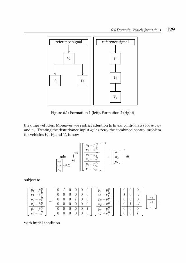
6.4 Example: Vehicle formations 129
reference signal reference signal
Vc
V1 V2
Vc
Vb
Va
Figure 6.1: Formation 1 (left), Formation 2 (right)
the other vehicles. Moreover, we restrict attention to linear control laws for a1, a2
and ac. Treating the disturbance input aRc as zero, the combined control problemfor vehicles V1, V2 and Vc is now
mina1
a2
ac
∈UCLSlin
∫ ∞0
∥∥∥∥∥∥∥∥∥∥∥∥
p1 − pR1v1 − vR1p2 − pR2v2 − vR2pc − pRcvc − vRc
∥∥∥∥∥∥∥∥∥∥∥∥
2
+
∥∥∥∥∥∥a1
a2
ac
∥∥∥∥∥∥2
dt,
subject top1 − pR1v1 − vR1p2 − pR2v2 − vR2pc − pRcvc − vRc
=
0 I 0 0 0 00 0 0 0 0 00 0 0 I 0 00 0 0 0 0 00 0 0 0 0 I0 0 0 0 0 0
p1 − pR1v1 − vR1p2 − pR2v2 − vR2pc − pRcvc − vRc
+
0 0 0I 0 −I0 0 00 I −I0 0 00 0 I
a1
a2
ac
,
with initial condition
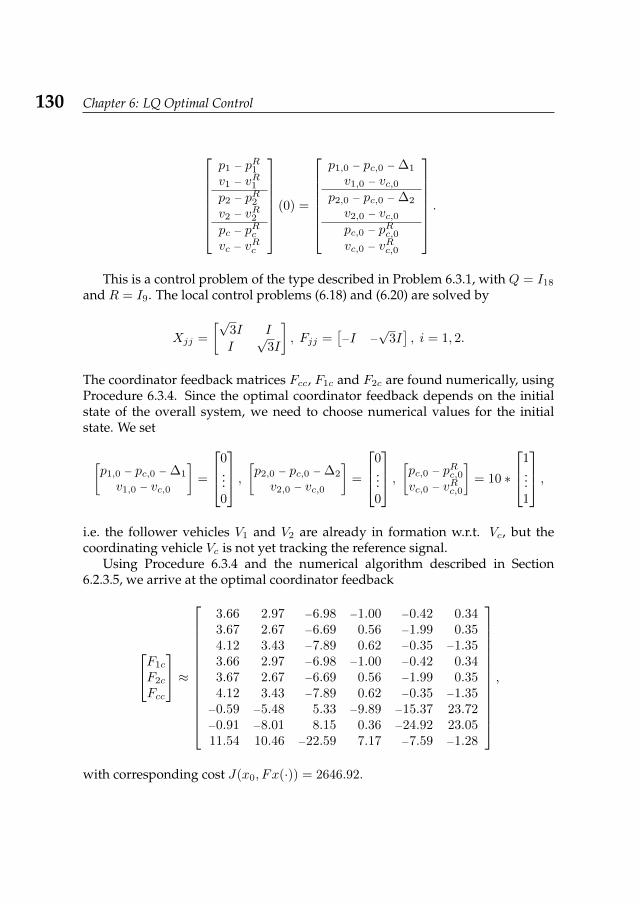
130 Chapter 6: LQ Optimal Control
p1 − pR1v1 − vR1p2 − pR2v2 − vR2pc − pRcvc − vRc
(0) =
p1,0 − pc,0 −∆1
v1,0 − vc,0p2,0 − pc,0 −∆2
v2,0 − vc,0pc,0 − pRc,0vc,0 − vRc,0
.
This is a control problem of the type described in Problem 6.3.1, with Q = I18
and R = I9. The local control problems (6.18) and (6.20) are solved by
Xjj =
[√3I I
I√
3I
], Fjj =
[−I −
√3I], i = 1, 2.
The coordinator feedback matrices Fcc, F1c and F2c are found numerically, usingProcedure 6.3.4. Since the optimal coordinator feedback depends on the initialstate of the overall system, we need to choose numerical values for the initialstate. We set
[p1,0 − pc,0 −∆1
v1,0 − vc,0
]=
0...0
, [p2,0 − pc,0 −∆2
v2,0 − vc,0
]=
0...0
, [pc,0 − pRc,0vc,0 − vRc,0
]= 10 ∗
1...1
,i.e. the follower vehicles V1 and V2 are already in formation w.r.t. Vc, but thecoordinating vehicle Vc is not yet tracking the reference signal.
Using Procedure 6.3.4 and the numerical algorithm described in Section6.2.3.5, we arrive at the optimal coordinator feedback
F1c
F2c
Fcc
≈
3.66 2.97 −6.98 −1.00 −0.42 0.343.67 2.67 −6.69 0.56 −1.99 0.354.12 3.43 −7.89 0.62 −0.35 −1.353.66 2.97 −6.98 −1.00 −0.42 0.343.67 2.67 −6.69 0.56 −1.99 0.354.12 3.43 −7.89 0.62 −0.35 −1.35−0.59 −5.48 5.33 −9.89 −15.37 23.72−0.91 −8.01 8.15 0.36 −24.92 23.0511.54 10.46 −22.59 7.17 −7.59 −1.28
,
with corresponding cost J(x0, Fx(·)) = 2646.92.
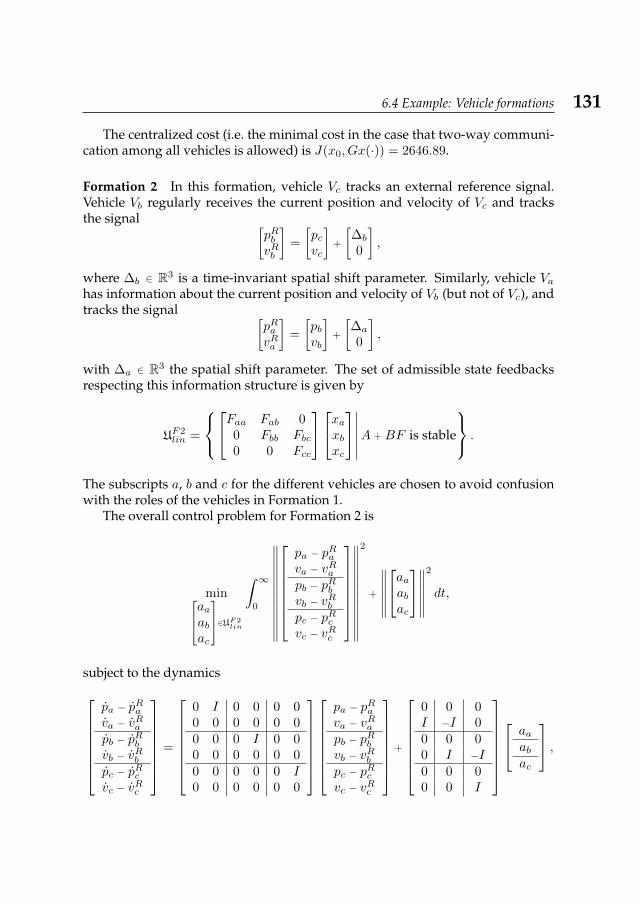
6.4 Example: Vehicle formations 131
The centralized cost (i.e. the minimal cost in the case that two-way communi-cation among all vehicles is allowed) is J(x0, Gx(·)) = 2646.89.
Formation 2 In this formation, vehicle Vc tracks an external reference signal.Vehicle Vb regularly receives the current position and velocity of Vc and tracksthe signal [
pRbvRb
]=
[pcvc
]+
[∆b
0
],
where ∆b ∈ R3 is a time-invariant spatial shift parameter. Similarly, vehicle Vahas information about the current position and velocity of Vb (but not of Vc), andtracks the signal [
pRavRa
]=
[pbvb
]+
[∆a
0
],
with ∆a ∈ R3 the spatial shift parameter. The set of admissible state feedbacksrespecting this information structure is given by
UF2lin =
Faa Fab 0
0 Fbb Fbc0 0 Fcc
xaxbxc
∣∣∣∣∣∣A + BF is stable
.
The subscripts a, b and c for the different vehicles are chosen to avoid confusionwith the roles of the vehicles in Formation 1.
The overall control problem for Formation 2 is
minaaabac
∈UF2lin
∫ ∞0
∥∥∥∥∥∥∥∥∥∥∥∥
pa − pRava − vRapb − pRbvb − vRbpc − pRcvc − vRc
∥∥∥∥∥∥∥∥∥∥∥∥
2
+
∥∥∥∥∥∥aaabac
∥∥∥∥∥∥2
dt,
subject to the dynamicspa − pRava − vRapb − pRbvb − vRbpc − pRcvc − vRc
=
0 I 0 0 0 00 0 0 0 0 00 0 0 I 0 00 0 0 0 0 00 0 0 0 0 I0 0 0 0 0 0
pa − pRava − vRapb − pRbvb − vRbpc − pRcvc − vRc
+
0 0 0I −I 00 0 00 I −I0 0 00 0 I
aaabac
,
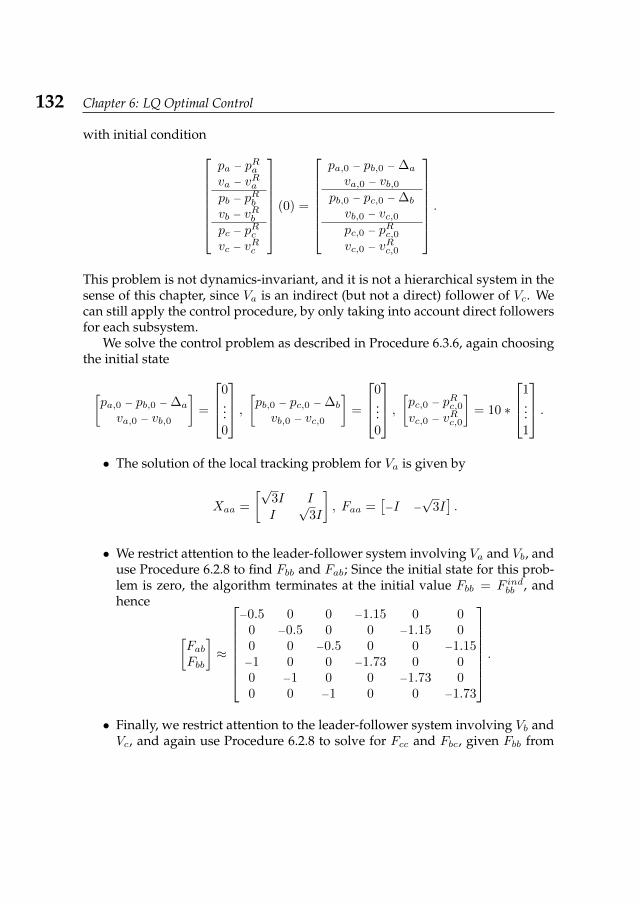
132 Chapter 6: LQ Optimal Control
with initial conditionpa − pRava − vRapb − pRbvb − vRbpc − pRcvc − vRc
(0) =
pa,0 − pb,0 −∆a
va,0 − vb,0pb,0 − pc,0 −∆b
vb,0 − vc,0pc,0 − pRc,0vc,0 − vRc,0
.
This problem is not dynamics-invariant, and it is not a hierarchical system in thesense of this chapter, since Va is an indirect (but not a direct) follower of Vc. Wecan still apply the control procedure, by only taking into account direct followersfor each subsystem.
We solve the control problem as described in Procedure 6.3.6, again choosingthe initial state
[pa,0 − pb,0 −∆a
va,0 − vb,0
]=
0...0
, [pb,0 − pc,0 −∆b
vb,0 − vc,0
]=
0...0
, [pc,0 − pRc,0vc,0 − vRc,0
]= 10 ∗
1...1
.• The solution of the local tracking problem for Va is given by
Xaa =
[√3I I
I√
3I
], Faa =
[−I −
√3I].
• We restrict attention to the leader-follower system involving Va and Vb, anduse Procedure 6.2.8 to find Fbb and Fab; Since the initial state for this prob-lem is zero, the algorithm terminates at the initial value Fbb = F indbb , andhence
[FabFbb
]≈
−0.5 0 0 −1.15 0 0
0 −0.5 0 0 −1.15 00 0 −0.5 0 0 −1.15−1 0 0 −1.73 0 00 −1 0 0 −1.73 00 0 −1 0 0 −1.73
.
• Finally, we restrict attention to the leader-follower system involving Vb andVc, and again use Procedure 6.2.8 to solve for Fcc and Fbc, given Fbb from
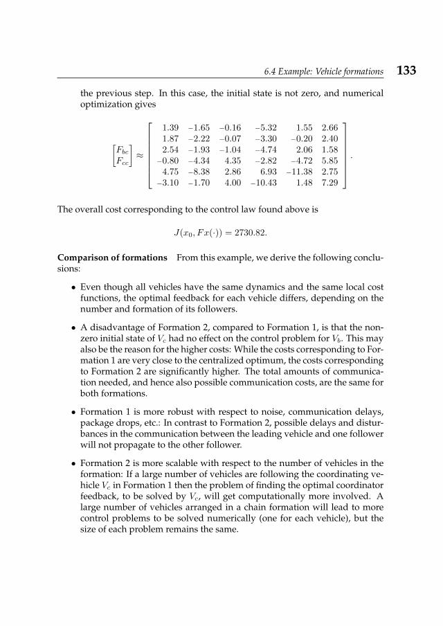
6.4 Example: Vehicle formations 133
the previous step. In this case, the initial state is not zero, and numericaloptimization gives
[FbcFcc
]≈
1.39 −1.65 −0.16 −5.32 1.55 2.661.87 −2.22 −0.07 −3.30 −0.20 2.402.54 −1.93 −1.04 −4.74 2.06 1.58−0.80 −4.34 4.35 −2.82 −4.72 5.85
4.75 −8.38 2.86 6.93 −11.38 2.75−3.10 −1.70 4.00 −10.43 1.48 7.29
.
The overall cost corresponding to the control law found above is
J(x0, Fx(·)) = 2730.82.
Comparison of formations From this example, we derive the following conclu-sions:
• Even though all vehicles have the same dynamics and the same local costfunctions, the optimal feedback for each vehicle differs, depending on thenumber and formation of its followers.
• A disadvantage of Formation 2, compared to Formation 1, is that the non-zero initial state of Vc had no effect on the control problem for Vb. This mayalso be the reason for the higher costs: While the costs corresponding to For-mation 1 are very close to the centralized optimum, the costs correspondingto Formation 2 are significantly higher. The total amounts of communica-tion needed, and hence also possible communication costs, are the same forboth formations.
• Formation 1 is more robust with respect to noise, communication delays,package drops, etc.: In contrast to Formation 2, possible delays and distur-bances in the communication between the leading vehicle and one followerwill not propagate to the other follower.
• Formation 2 is more scalable with respect to the number of vehicles in theformation: If a large number of vehicles are following the coordinating ve-hicle Vc in Formation 1 then the problem of finding the optimal coordinatorfeedback, to be solved by Vc, will get computationally more involved. Alarge number of vehicles arranged in a chain formation will lead to morecontrol problems to be solved numerically (one for each vehicle), but thesize of each problem remains the same.
134 Chapter 6: LQ Optimal Control
LQ Control with Event-based Feedback 7As an alternative to the control synthesis procedure developed in the previouschapter, we now introduce and analyze a control law which uses event-basedbottom-to-top feedback.
This chapter was published as [26].
7.1 IntroductionIn this chapter, we derive a control law for coordinated linear systems which com-bines linear state feedbacks with event-based feedbacks. While the linear feed-backs respect the system’s top-to-bottom information structure, the event-basedfeedbacks correspond to occasional bottom-to-top communication. In Section 7.2the control problem we consider is formulated for the special case involving onlyone subsystem. Our control law with event-based feedback is introduced in Sec-tion 7.3, and its extension to larger hierarchical systems is discussed in Section7.4. Finally, the performance of the control law is illustrated in an example inSection 7.5.
7.2 Problem formulationWe will first restrict our attention to leader-follower systems, i.e. coordinated lin-ear systems with only one subsystem, of the form[
xsxc
]=
[Ass Asc0 Acc
] [xsxc
]+
[Bss Bsc0 Bcc
] [usuc
],
[xs(t0)xc(t0)
]=
[xs,0xc,0
]. (7.1)
The subscript c stands for ‘coordinator’, and s stands for ‘subsystem’. The exten-sion of our results to larger hierarchical systems is discussed in Section 7.4.
For a system of the form (7.1), we define the following infinite-horizonquadratic cost function:
J (x0, u(·)) =
∫ ∞t0
([xsxc
]T [Qss 00 Qcc
] [xsxc
]+
[usuc
]T [Rss 00 Rcc
] [usuc
])dt, (7.2)
where Q =
[Qss 00 Qcc
]≥ 0 and R =
[Rss 00 Rcc
]> 0.
136 Chapter 7: LQ Control with Event-based Feedback
We consider the following sets of admissible control laws:
U↑↓=
[us(t, xs(t), xc(t))uc(t, xs(t), xc(t))
]∣∣∣∣us, uc piecewise continuous in t,
U↓ =
[us(t, xs(t), xc(t))uc(t, xs,0, xc(t))
]∣∣∣∣us, uc piecewise continuous in t,
Ur,β=
[us(t, xs(t), xc(t))uc(t, xs,j , xc(t))
]∣∣∣∣ us, uc piecewise continuous in t,xs,j = xs(tj), tj ≤ t, t0, t1, . . . , tn ⊂ [t0,∞)
.
The subscripts r and β are used here to comply with our notation in Section 7.3,where we introduce a control law with event-based feedback xs,jj=0,...,n, usinga guard condition which depends on two parameters r and β. Note that U↓ ⊆Ur,β ⊆ U↑↓.
In this chapter, we will consider the following problem:
7.2.1. Problem. Let a system of the form (7.1) and a cost function of the form (7.2)be given. Assume that ([
Ass Asc0 Acc
],
[Bss Bsc0 Bcc
])is a stabilizable pair and that([
Qss 00 Qcc
],
[Ass Asc0 Acc
])is a detectable pair. Minimize the cost over Ur,β , i.e. find
minu(·)∈Ur,β
J (x0, u(·)) . (7.3)
In Section 7.3 we introduce a piecewise-linear control law in Ur,β which leadsto a finite cost for all r ≥ 0, and approximates the centralized optimum (and hencealso the solution of (7.3)) for r → 0.
7.3 Control with event-based feedbackFor the purpose of the following derivation, we assume that xc(t) 6= 0 for allt ≥ t0. Set
T (t) =xs(t)xc(t)
T
xc(t)Txc(t),
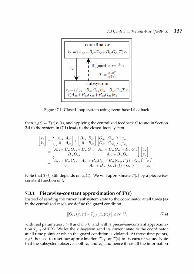
7.3 Control with event-based feedback 137
Figure 7.1: Closed-loop system using event-based feedback
then xs(t) = T (t)xc(t), and applying the centralized feedback G found in Section2.4 to the system in (7.1) leads to the closed-loop system[
xsxc
]=
([Ass Asc0 Acc
]+
[Bss Bsc0 Bcc
] [Gss GscGcs Gcc
])[xsxc
]=
[Ass + BssGss + BscGcs Asc + BssGsc + BscGcc
BccGcs Acc + BccGcc
] [xsxc
]=
[Ass + BssGss Asc + BssGsc + Bsc(GcsT (t) + Gcc)
0 Acc + Bcc (GcsT (t) + Gcc)
] [xsxc
].
Note that T (t) still depends on xs(t). We will approximate T (t) by a piecewise-constant function of t.
7.3.1 Piecewise-constant approximation of T (t)Instead of sending the current subsystem state to the coordinator at all times (asin the centralized case), we define the guard condition∥∥Gcs (xs(t) − Tj(t−)xc(t))∥∥ ≤ re−βt, (7.4)
with real parameters r ≥ 0 and β > 0, and with a piecewise-constant approxima-tion Tj(t) of T (t). We let the subsystem send its current state to the coordinatorat all time points at which the guard condition is violated. At those time points,xs(t) is used to reset our approximation Tj(t) of T (t) to its current value. Notethat the subsystem observes both xs and xc, and hence it has all the information
138 Chapter 7: LQ Control with Event-based Feedback
necessary to check the guard condition at each step. Whenever the guard con-dition is satisfied, the coordinator uses the most recent approximation of T (t),which was computed the last time the subsystem sent its state to the coordinator(or at t0). The control law resulting from this approximation is of the form
gr,β(x(t)) =
[Gssxs(t) + Gscxc(t)(GcsTj(t) + Gcc
)xc(t)
],
where Tj is given by
Tj(t+) =
Tj(t−) if guard ≤ re−βt
xs(t)xTc (t)
xTc (t)xc(t)if guard > re−βt
,
and the guard is given by
guard =∥∥Gcs (xs(t) − Tj(t−)xc(t))∥∥ .
This control law is illustrated in Figure 7.1.
7.3.2 Results on the performance of gr,βOur first result on the performance of the control law gr,β states that it leads to anexponentially stable system.
7.3.1. Proposition. For any r ≥ 0 and β > 0, applying the control law gr,β(x(·)) to(7.1) leads to an exponentially stable closed-loop system.
Proof. Applying gr(x(·)) leads to the closed-loop system
x =
(A + BG +
[BscBcc
]Gcs
[−I Tj
])x
= (A + BG)x +
[BscBcc
]Gcs (Tjxc − xs)
and hence the state trajectory is described by
x(t) = e(A+BG)(t−t0)x0 +
∫ t
t0
e(A+BG)(t−τ)
[BscBcc
]Gcs
(Tj(τ)xc(τ) − xs(τ)
)dτ.
Since A + BG is stable, there exist constants M > 0 and α > 0 such that∥∥∥e(A+BG)∆t
∥∥∥ ≤Me−α∆t ∀∆t ≥ 0.
7.3 Control with event-based feedback 139
We pick α 6= β. Now we have
‖x(t)‖ ≤∥∥∥e(A+BG)(t−t0)
∥∥∥ ‖x0‖
+
∫ t
t0
∥∥∥e(A+BG)(t−τ)∥∥∥∥∥∥∥[BscBcc
]∥∥∥∥ ∥∥Gcs (Tj(τ)xc(τ) − xs(τ))∥∥ dτ
≤Me−α(t−t0) ‖x0‖ +
∫ t
t0
Me−α(t−τ)
∥∥∥∥[BscBcc
]∥∥∥∥ re−βτdτ= Me−α(t−t0) ‖x0‖ + M
∥∥∥∥[BscBcc
]∥∥∥∥ rα − β
(e−βt − e−α(t−t0)−βt0
),
which goes to 0 exponentially as t→∞.
The following result states that the increase in the total cost, resulting fromusing a piecewise-constant approximation for T (t) instead of its exact value, isbounded.
7.3.2. Proposition. For any r > 0 and β > 0, the difference between the cost correspond-ing to gr,β and the centralized cost is bounded by
J(x0, gr,β(x(·))) − J(x0, Gx(·)) ≤∥∥∥R 1
2
∥∥∥2
r2 e−2βt0
2β. (7.5)
Proof. For simplicity, we denote the difference of the control feedbacks by
Gj =
[0 0
−Gcs GcsTj
].
Let t ≥ tj , and suppose that the most recent feedback from the subsystem wassent at time tj . Then the system dynamics over [tj , t] are linear and time-invariant,and hence the cost corresponding to the control law gr,β over the interval [tj , t]is given by xT (tj)Yjx(tj) − xT (t)Yjx(t), where Yj is the solution of the Lyapunovequation
(A + B
(G + Gj
))TYj + Yj
(A + B
(G + Gj
))+ Q +
(G + Gj
)TR(G + Gj
)= 0.
The cost corresponding to the centralized control law u(·) = Gx(·) was derivedin Section 2.4: We have J(x0, Gx(·)) = xT0 Xx0, where X is the unique solution ofXBR−1BTX − ATX − XA − Q = 0 such that G = −R−1BTX is stabilizing (i.e.
140 Chapter 7: LQ Control with Event-based Feedback
A − BR−1BTX is stable). Using BTX = −RG, and in analogy with the proof ofTheorem 2.4.1, we now derive a Lyapunov equation for Yj −X :
(A + B
(G + Gj
))T(Yj −X) + (Yj −X)
(A + B
(G + Gj
))= −Q −
(G + Gj
)TR(G + Gj
)− (A + BG)
TX −X (A + BG) − GTj B
TX −XBGj
= −(G + Gj
)TR(G + Gj
)+ GTRG + GTj RG + GTRGj
= −GTj RGj .
Using this, we can now derive an expression for the difference in cost over[tj , tj+1]:(xT (tj)Yjx (tj) − x
T (tj+1)Yjx (tj+1))−(xT (tj)Xx (tj) − x
T (tj+1)Xx (tj+1))
= xT (tj) (Yj −X)x (tj) − xT (tj+1) (Yj −X)x (tj+1)
=
∫ tj+1
tj
−d
dt
(xT (t) (Yj −X)x (t)
)dt
=
∫ tj+1
tj
−(xT (t)
((A + B
(G+Gj
))(Y −X) + (Y −X)
(A + B
(G+Gj
)))x (t)
)dt
=
∫ tj+1
tj
(xT (t) GTj RGjx (t)
)dt
=
∫ tj+1
tj
∥∥∥R1/2Gjx (t)∥∥∥2
dt,
where x(·) is the state trajectory of the closed-loop system obtained from applyingthe control law gr,β = G + Gj . Since x(·) is exponentially stable by Proposition7.3.1, the last derivation also holds over [tn+1,∞]. Now
J (x0, gr,β(x(·))) − J (x0, Gx(·))
=n∑j=0
∫ tj+1
tj
∥∥∥R 12Gcs
[−I Tj
]x (t)
∥∥∥2
dt +
∫ ∞tn+1
∥∥∥R 12Gcs
[−I Tn+1
]x (t)
∥∥∥2
dt
≤n∑j=0
∫ tj+1
tj
∥∥∥R 12
∥∥∥2
r2e−2βtdt +
∫ ∞tn+1
∥∥∥R 12
∥∥∥2
r2e−2βtdt
=∥∥∥R 1
2
∥∥∥2
r2 e−2βt0
2β.
7.3 Control with event-based feedback 141
Note that Proposition 7.3.2 also implies that
limr→0
J(x0, gr,β(x(·))) = J(x0, Gx(·)),
i.e. for any β > 0 the cost corresponding to gr,β approaches the optimal central-ized cost for r → 0.
For r → ∞, we have Ur,β → U↓, but g∞,β(x(·)) is not the optimal control lawover U↓ (in fact, it is not even the optimal linear control law over U↓, see Chapter6). Hence, while gr,β leads to a good closed-loop performance for small r, thereare better options for large r.
The following proposition verifies a property one would intuitively require ofa coordination control law: If the different parts of a system are fully decoupled(i.e. the coordinator state and input do not influence the subsystem state) then thecontrol law gr,β reduces to the optimal control law of the centralized case.
7.3.3. Proposition. If Asc = 0 and Bsc = 0 then gr,β(x(t)) = Gx(t) for all t ≥ t0,r ≥ 0 and β ≥ 0.
Proof. For Asc = 0 and Bsc = 0, the open-loop system is completely decoupled.Since Q and R are also chosen block-diagonal in (7.2), the solution of the Ricattiequation (2.10) is block-diagonal, and hence so is G = −R−1BTX . But then Gcs =0, which gives
∥∥Gcs(xs(t) − Tj(t−)xc(t))∥∥ = 0, and hence
uc(t, xs,j , xc(t)) = Gccxc(t) = uc(t, xs,0, xc(t))
for all r and β.
The following result concerning the time span between two subsequent re-sets of Tj has been observed for many randomly generated control problems insimulations, but has not yet been proven:
7.3.4. Conjecture. Let a system of the form (7.1) and a cost function of the form (7.2) begiven, and let
α = min |Re(λ)||λ ∈ σ(A + BG) .
(a) For all r > 0 and β ∈ (0, α) there exists ε > 0 such that ‖tj+1 − tj‖ > ε for allj ≥ 0.
(b) For all r > 0 there exist βmax ∈ (0, α) and tN > t0 such that the guard conditionis satisfied for all β ∈ (0, βmax) and t > tN .
Part (a) excludes infinite resets in finite time, and part (b) states that for βsmall enough, there are only finitely many resets. Assuming that Conjecture 7.3.4holds, we have that gr,β ∈ Ur,β . While part (a) is crucial in establishing that gr,β is
142 Chapter 7: LQ Control with Event-based Feedback
useful in practice, part (b) can easily be circumvented by redefining the set Ur,βto allow for countably many resets.1
7.4 Extension to hierarchical systemsThis section explains how to extend the results of Section 7.3 to more generalhierarchical systems with a top-to-bottom information structure. The cases of asystem with two subsystems and a system with three layers are discussed below.Control laws for other hierarchical systems can then be derived by combiningthese cases.
7.4.1 Systems with several subsystemsIn the following, we illustrate how to extend the control law gr,β introduced inSection 7.3 to a coordinated linear system with two subsystems and a coordinator.
We will consider the following system and cost function:x1
x2
xc
=
A11 0 A1c
0 A22 A2c
0 0 Acc
x1
x2
xc
+
B11 0 B1c
0 B22 B2c
0 0 Bcc
u1
u2
uc
,x1(t0)x2(t0)xc(t0)
=
x1,0
x2,0
xc,0
,J(x0, u(·))
=
∫ ∞t0
x1
x2
xc
T Q11 0 00 Q22 00 0 Qcc
x1
x2
xc
+
u1
u2
uc
T R11 0 00 R22 00 0 Rcc
u1
u2
uc
dt.
The optimal centralized control law Gx(·) ∈ U↑↓ is again linear and time-invariant, with G an unstructured matrix. We again approximate Gx(·) bya structure-preserving piecewise-linear feedback, i.e. a feedback of the form? 0 ?
0 ? ?0 0 ?
x(·), by using piecewise-constant approximations of the matrices
Ti(t) =xi(t)x
Tc (t)
xTc (t)xc(t), for i = 1, 2.
1In fact, if part (a) is false then applying gr,β may lead to Zeno behavior in theory – in practicethe system will be unable to execute the control law, and will lose stability. Since no applicationis designed to run for infinite time, part (b) is irrelevant in practice; it may however be useful forbounding the long-run communication costs.
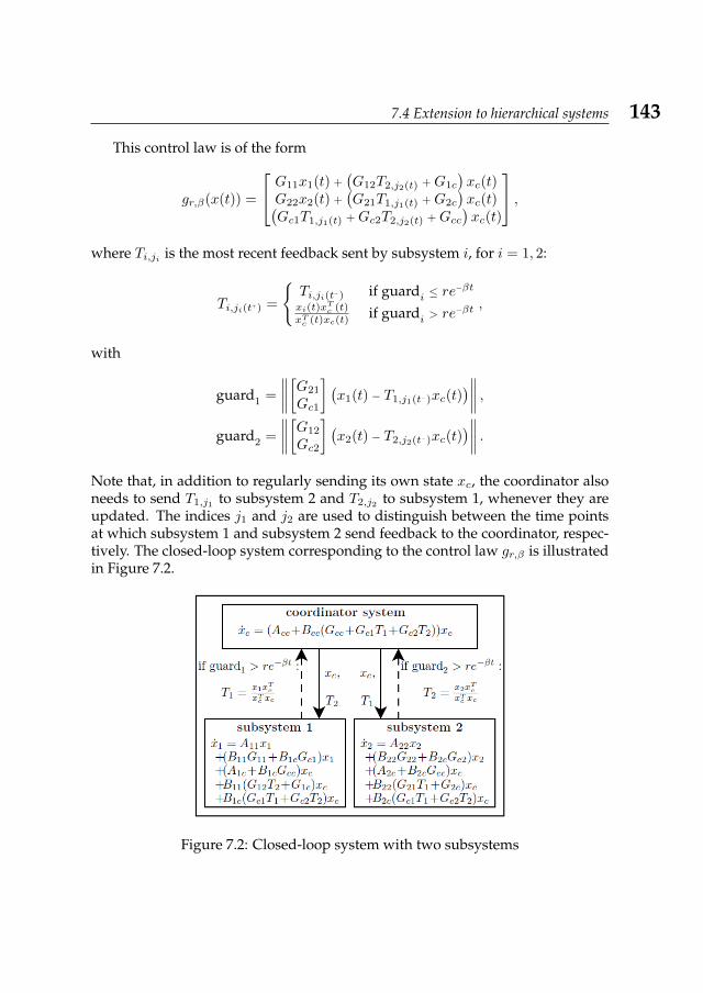
7.4 Extension to hierarchical systems 143
This control law is of the form
gr,β(x(t)) =
G11x1(t) +(G12T2,j2(t) + G1c
)xc(t)
G22x2(t) +(G21T1,j1(t) + G2c
)xc(t)(
Gc1T1,j1(t) + Gc2T2,j2(t) + Gcc)xc(t)
,where Ti,ji is the most recent feedback sent by subsystem i, for i = 1, 2:
Ti,ji(t+) =
Ti,ji(t−) if guardi ≤ re
−βt
xi(t)xTc (t)
xTc (t)xc(t)if guardi > re
−βt ,
with
guard1 =
∥∥∥∥[G21
Gc1
] (x1(t) − T1,j1(t−)xc(t)
)∥∥∥∥ ,guard2 =
∥∥∥∥[G12
Gc2
] (x2(t) − T2,j2(t−)xc(t)
)∥∥∥∥ .Note that, in addition to regularly sending its own state xc, the coordinator alsoneeds to send T1,j1 to subsystem 2 and T2,j2 to subsystem 1, whenever they areupdated. The indices j1 and j2 are used to distinguish between the time pointsat which subsystem 1 and subsystem 2 send feedback to the coordinator, respec-tively. The closed-loop system corresponding to the control law gr,β is illustratedin Figure 7.2.
Figure 7.2: Closed-loop system with two subsystems
144 Chapter 7: LQ Control with Event-based Feedback
Proposition 7.3.1 can easily be extended to show that this closed-loop systemis exponentially stable. Let x(t) describe the state trajectory obtained by applyinggr,β , then we can bound ‖Gx(t) − gr,β(x(t))‖2 in a similar manner as in Proposi-tion 7.3.2:
‖Gx(t) − gr,β(x(t))‖2 =
∥∥∥∥∥∥ 0 −G12 G12T2
−G21 0 G21T1
−Gc1 −Gc2 Gc1T1 + Gc2T2
x(t)
∥∥∥∥∥∥2
=
∥∥∥∥∥∥ 0G21
Gc1
[−I 0 T1
]x(t) +
G12
0Gc2
[0 −I T2
]x(t)
∥∥∥∥∥∥2
≤ 2
∥∥∥∥[G21
Gc1
](x1(t) − T1xc(t))
∥∥∥∥2
+ 2
∥∥∥∥[G12
Gc2
](x2(t) − T2xc(t))
∥∥∥∥2
≤ 4r2e−2βt.
Using this bound and the same argument as in the proof of Proposition 7.3.2, wefind that
J(x0, gr,β(x(·))) − J(x0, Gx(·)) ≤ 4∥∥∥R 1
2
∥∥∥2
r2 e−2βt0
2β.
7.4.2 Systems with several layersWe consider the following system and cost function:x1
x2
x3
=
A11 A12 A13
0 A22 A23
0 0 A33
x1
x2
x3
+
B11 B12 B13
0 B22 B23
0 0 B33
u1
u2
u3
,J(x0, u(·))
=
∫ ∞t0
x1
x2
x3
T Q11 0 00 Q22 00 0 Q33
x1
x2
x3
+
u1
u2
u3
T R11 0 00 R22 00 0 R33
u1
u2
u3
dt,
with initial state
x1(t0)x2(t0)x3(t0)
=
x1,0
x2,0
x3,0
. Each subsystem now corresponds to one
layer in the hierarchy. We define the functions
T12 =x1x
T2
xT2 x2, T13 =
x1xT3
xT3 x3, T23 =
x2xT3
xT3 x3,
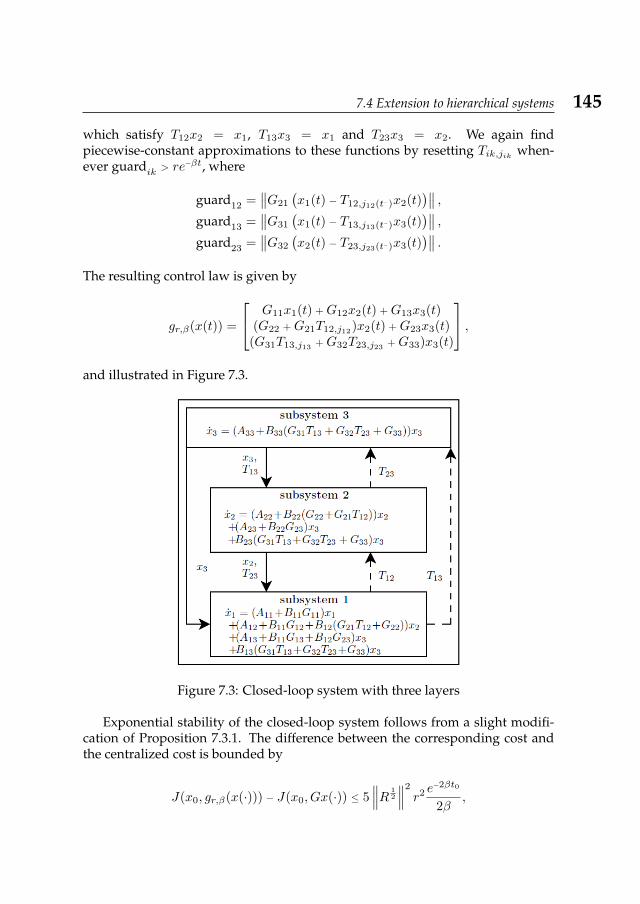
7.4 Extension to hierarchical systems 145
which satisfy T12x2 = x1, T13x3 = x1 and T23x3 = x2. We again findpiecewise-constant approximations to these functions by resetting Tik,jik when-ever guardik > re
−βt, where
guard12 =∥∥G21
(x1(t) − T12,j12(t−)x2(t)
)∥∥ ,guard13 =
∥∥G31
(x1(t) − T13,j13(t−)x3(t)
)∥∥ ,guard23 =
∥∥G32
(x2(t) − T23,j23(t−)x3(t)
)∥∥ .The resulting control law is given by
gr,β(x(t)) =
G11x1(t) + G12x2(t) + G13x3(t)(G22 + G21T12,j12)x2(t) + G23x3(t)
(G31T13,j13 + G32T23,j23 + G33)x3(t)
,and illustrated in Figure 7.3.
Figure 7.3: Closed-loop system with three layers
Exponential stability of the closed-loop system follows from a slight modifi-cation of Proposition 7.3.1. The difference between the corresponding cost andthe centralized cost is bounded by
J(x0, gr,β(x(·))) − J(x0, Gx(·)) ≤ 5∥∥∥R 1
2
∥∥∥2
r2 e−2βt0
2β,
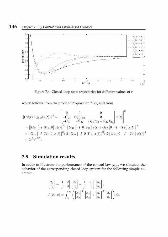
146 Chapter 7: LQ Control with Event-based Feedback
Figure 7.4: Closed-loop state trajectories for different values of r
which follows from the proof of Proposition 7.3.2, and from
‖Gx(t) − gr,β(x(t))‖2 =
∥∥∥∥∥∥ 0 0 0−G21 G21T12 0−G31 −G32 G31T13 + G32T23
x(t)
∥∥∥∥∥∥2
=∥∥G21
[−I T12 0
]x(t)
∥∥2+∥∥G31
[−I 0 T13
]x(t) + G32
[0 −I −T23
]x(t)
∥∥2
≤∥∥G21
[−I T12 0
]x(t)
∥∥2+ 2∥∥G31
[−I 0 T13
]x(t)
∥∥2+ 2∥∥G32
[0 −I −T23
]x(t)
∥∥2
≤ 5r2e−2βt.
7.5 Simulation resultsIn order to illustrate the performance of the control law gr,β , we simulate thebehavior of the corresponding closed-loop system for the following simple ex-ample: [
xsxc
]=
[1 20 3
] [xsxc
]+
[1 −10 1
] [usuc
],
J (x0, u) =
∫ ∞t0
([xsxc
]T [xsxc
]+
[usuc
]T [usuc
])dt,
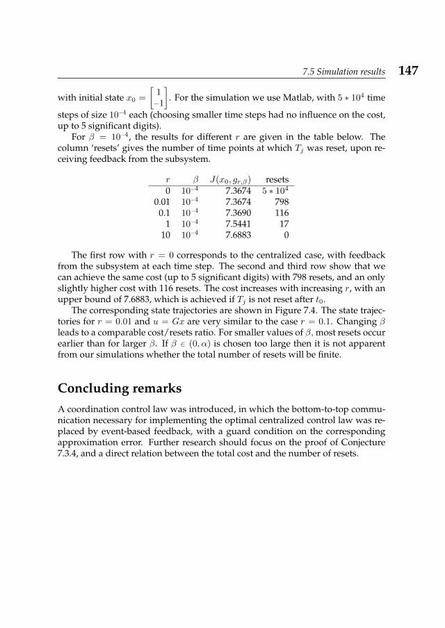
7.5 Simulation results 147
with initial state x0 =
[1−1
]. For the simulation we use Matlab, with 5 ∗ 104 time
steps of size 10−4 each (choosing smaller time steps had no influence on the cost,up to 5 significant digits).
For β = 10−4, the results for different r are given in the table below. Thecolumn ‘resets’ gives the number of time points at which Tj was reset, upon re-ceiving feedback from the subsystem.
r β J(x0, gr,β) resets0 10−4 7.3674 5 ∗ 104
0.01 10−4 7.3674 7980.1 10−4 7.3690 116
1 10−4 7.5441 1710 10−4 7.6883 0
The first row with r = 0 corresponds to the centralized case, with feedbackfrom the subsystem at each time step. The second and third row show that wecan achieve the same cost (up to 5 significant digits) with 798 resets, and an onlyslightly higher cost with 116 resets. The cost increases with increasing r, with anupper bound of 7.6883, which is achieved if Tj is not reset after t0.
The corresponding state trajectories are shown in Figure 7.4. The state trajec-tories for r = 0.01 and u = Gx are very similar to the case r = 0.1. Changing βleads to a comparable cost/resets ratio. For smaller values of β, most resets occurearlier than for larger β. If β ∈ (0, α) is chosen too large then it is not apparentfrom our simulations whether the total number of resets will be finite.
Concluding remarksA coordination control law was introduced, in which the bottom-to-top commu-nication necessary for implementing the optimal centralized control law was re-placed by event-based feedback, with a guard condition on the correspondingapproximation error. Further research should focus on the proof of Conjecture7.3.4, and a direct relation between the total cost and the number of resets.
148 Chapter 7: LQ Control with Event-based Feedback
Case Studies 8In this chapter, two case studies for coordination control are described: Section8.1 deals with a formation flying problem for autonomous underwater vehicles,and Section 8.2 discusses a coordination problem for two ramp metering devicesat neighboring highway on-ramps.
8.1 Formation flying for AUVsThis section describes a coordination control approach to formation flying forAUVs, and was published as [24].
8.1.1 IntroductionThis section describes a case study for coordination control, involving severalautonomous underwater vehicles (AUVs): One AUV or surface vehicle shouldtrack an external reference signal, and two AUVs should follow the first vehiclein formation. This case study is strongly related to the problem statement of for-mation flying for AUVs formulated in [59]. The similar problem of coordinatedpath following control for AUVs is discussed in e.g. [11], and other approachesto formation flying using leader-follower structures are found in e.g. [7], [32].
The purpose of this case study is, on the one hand, to illustrate the theory ofcoordination control developed in this thesis, and on the other hand, to providea computationally efficient control algorithm for the problem of formation flyingfor AUVs.
The control problem considered in this paper consists of three tracking prob-lems, coupled by the formation to be kept, and subject to fixed bounds on thespeed and acceleration of each vehicle, random waves and currents, and errorsand delays in the communication among the vehicles.
Our approach adopts the linearized version of the model from [59]. In [59],a more general version of this problem is formulated, and solved using moving-horizon model predictive control on a linearized version of the model. While thisapproach leads to very good control laws, the on-line computations necessary forimplementing these control laws exceed the on-board processing power of theAUVs considered in this setting.
The novelty of our approach lies in restricting the communication among theAUVs to a minimum by imposing a hierarchical structure on the set of vehicles,and then using LQ optimal control to solve each tracking problem separately. Thenavigation and communication constraints are taken into account after findingthe optimal control laws. This leads to a control law which can be implementedwith very little computational effort.
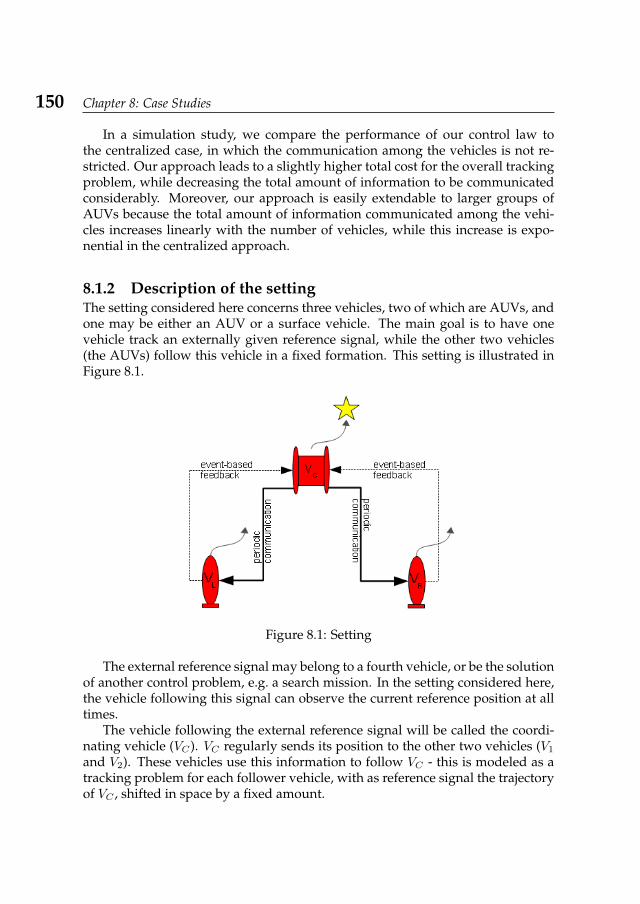
150 Chapter 8: Case Studies
In a simulation study, we compare the performance of our control law tothe centralized case, in which the communication among the vehicles is not re-stricted. Our approach leads to a slightly higher total cost for the overall trackingproblem, while decreasing the total amount of information to be communicatedconsiderably. Moreover, our approach is easily extendable to larger groups ofAUVs because the total amount of information communicated among the vehi-cles increases linearly with the number of vehicles, while this increase is expo-nential in the centralized approach.
8.1.2 Description of the settingThe setting considered here concerns three vehicles, two of which are AUVs, andone may be either an AUV or a surface vehicle. The main goal is to have onevehicle track an externally given reference signal, while the other two vehicles(the AUVs) follow this vehicle in a fixed formation. This setting is illustrated inFigure 8.1.
Figure 8.1: Setting
The external reference signal may belong to a fourth vehicle, or be the solutionof another control problem, e.g. a search mission. In the setting considered here,the vehicle following this signal can observe the current reference position at alltimes.
The vehicle following the external reference signal will be called the coordi-nating vehicle (VC). VC regularly sends its position to the other two vehicles (V1
and V2). These vehicles use this information to follow VC - this is modeled as atracking problem for each follower vehicle, with as reference signal the trajectoryof VC , shifted in space by a fixed amount.
8.1 Formation flying for AUVs 151
All vehicles are subject to currents and disturbances, and their velocities andaccelerations are bounded in norm. Because of these restrictions, it may not al-ways be possible for the vehicles to successfully track their reference trajectories.This leads to two possible problems: The follower vehicles V1 and V2 might fail tostay in formation (in the worst case, they might get lost), or the vehicles might col-lide. These two problems necessitate some form of communication from V1 andV2 to VC in the case that the control objectives cannot be met. Since underwatercommunication is extremely limited, we opt for a form of event-based commu-nication from V1 and V2 to VC in exceptional circumstances: At each time step,each follower vehicle checks whether its distance to its reference position exceedsa fixed limit. This can be done internally and without additional communicationsince their reference position is communicated by VC anyway. In the event thata vehicle exceeds the limit, it sends its actual position to the coordinating vehi-cle VC , which then takes measures to avoid collisions, or one vehicle being leftbehind.
Underwater communication is modeled as being subject to random delaysand packet losses. All messages sent are time-stamped, which means that at thetime a message is received, the recipient knows when the message was sent. Thecorresponding observer can then recompute its current estimate, starting fromthe time given in the time stamp. The clock drift among the different vehicles isbounded for missions of limited duration, and will be ignored here.
In the setting described here, the coordinating vehicle VC has to communicateits position regularly, while the other vehicles V1 and V2 do not. This means thatVC needs to use much more of its resources for communication. One possibleoption for ensuring that the resources of all vehicles are used in a more balancedway is to switch roles among the vehicles from time to time. In the case thatVC is a different type of vehicle than V1 and V2 (e.g. VC is a ship, or an under-water vehicle with more energy available), this imbalance in the communicationrequirements is actually desirable.
For the purpose of comparing performances, a second setting will be con-sidered, in which all vehicles can communicate with one another at all times.However, the communication is subject to the same delays and packet losses asdescribed above.
8.1.3 Model with communication constraintsFor ease of implementation, all dynamics involved will be approximated bydiscrete-time1 linear dynamical systems, as derived in [59]. To justify this choice,we note that a linearizing feedback is commonly applied to the AUVs by a lower-level controller. The approximation errors are modeled as disturbances, together
1The discrete-time approximation of a coordinated linear system is obtained by replacing x withx(t + 1) − x(t). The sparsity structure of the system matrices, which characterizes coordinated linearsystems, remains unchanged.
152 Chapter 8: Case Studies
with possible currents and other external disturbances. All disturbances are mod-eled as being zero-mean disturbances in the long run.
The following notation will be used:
• VC : coordinating vehicle
• V1, V2: vehicles following VC
• RC : external reference signal to be tracked by VC
• R1, R2: reference signals to be tracked by V1 and V2
• p ∈ R3: position
• s ∈ R3: velocity
• a ∈ R3: acceleration
• w ∈ R3: disturbances
• p, s ∈ R3: observer estimates for position and velocity
• ∆1,∆2 ∈ R3: desired relative positions of V1 and V2 with respect to theposition of VC
• τ ∈ (1,∞) : a time constant
For each vehicle, the acceleration is the control input. The disturbances are mod-eled as velocities, and affect only the change in position, not the change in veloc-ity.
These variables and their interconnections, in the case with communicationconstraints, are illustrated in Figure 8.2.
For the external reference system RC , we use an internal model with the fol-lowing dynamics:[
pRCsRC
](t + 1) =
[I I0 τ−1
τ I
] [pRCsRC
](t) +
[01τ I
]aRC (t) +
[I0
]wRC (t).
The state variables of this internal model are the position pRC and velocity sRCof RC , and the acceleration aRC is the control input. The disturbance wRC is anuncontrollable input; including wRC in the dynamics of the reference system isrealistic if RC is an actual vehicle or target to be tracked, it does not make senseif RC is a virtual system (e.g. the solution of a control problem).
All vehicles V1, V2 and VC have the following dynamics, derived in [59]:[pVjsVj
](t + 1) =
[I I0 τ−1
τ I
] [pVjsVj
](t) +
[01τ I
]aVj (t) +
[I0
]wVj (t),
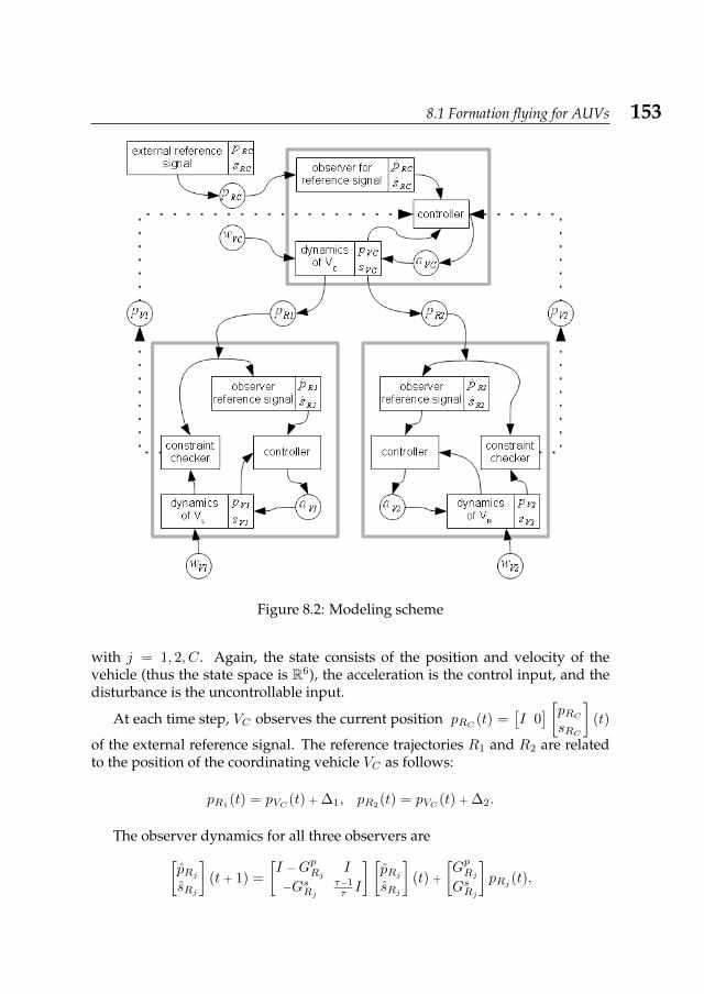
8.1 Formation flying for AUVs 153
Figure 8.2: Modeling scheme
with j = 1, 2, C. Again, the state consists of the position and velocity of thevehicle (thus the state space is R6), the acceleration is the control input, and thedisturbance is the uncontrollable input.
At each time step, VC observes the current position pRC (t) =[I 0] [pRCsRC
](t)
of the external reference signal. The reference trajectories R1 and R2 are relatedto the position of the coordinating vehicle VC as follows:
pR1(t) = pVC (t) + ∆1, pR2
(t) = pVC (t) + ∆2.
The observer dynamics for all three observers are[pRjsRj
](t + 1) =
[I −GpRj I
−GsRjτ−1τ I
] [pRjsRj
](t) +
[GpRjGsRj
]pRj (t),
154 Chapter 8: Case Studies
j = 1, 2, C, with pRj denoting the observations of the actual reference positions.The error dynamics are
[perrRjserrRj
](t + 1) =
[I −GpRj I
−GsRjτ−1τ I
] [perrRjserrRj
](t) +
[01τ I
]aRj (t) +
[I0
]wRj (t),
where aRC and wRC are the acceleration and disturbance of the external referencesignal, and aR1 = aR2 = aVC and wR1 = wR2 = wVC because the reference sys-tems of the follower vehicles have the same dynamics as the coordinating vehicle.aR1
, aR2, wR1
and wR2only play a role in the observer errors; they are not used
on-board by V1 or V2. GpRj and GsRj are appropriate observer gains.Combining these variables and dynamics, we arrive at the open-loop system
given in Table 8.1. This is an affine system because the last term, involving ∆1
and ∆2, is constant.The state variables pV1 , sV1 , pR1 , sV1 belong to vehicle V1, the variables pV2 ,
sV2 , pR2 , sR2 are the state variables of vehicle V2, and the state variables pVC , sVC ,pVC , sVC belong to the coordinating vehicle VC . For each vehicle, the state spacedimension is 12, and the state space of the overall system has dimension 36.
The internal model used for the external reference signal is not included inthis open-loop system because the state variables of the external reference signalare not located in either of the vehicles. The accelerations aV1 , aV2 , aVC are thecontrol inputs, the variables wV1
, wV2, wVC , pRC are the external inputs, and ∆1,
∆2 are fixed parameters.The open-loop system in Table 8.1 is a coordinated affine system. The coor-
dinating vehicle corresponds to the coordinator of a coordinated system, and thefollower vehicles correspond to the subsystems. Coordinated systems have theproperty that the coordinator influences the subsystems, while the subsystemshave no influence on the coordinator, or on each other. In this case study, thiscorresponds to the coordinating vehicle sending its position to the other vehiclesregularly. The event-based feedback from the other vehicles to the coordinatingvehicle does not comply with the structure of a coordinated system, and hencethe closed-loop system will only correspond to a coordinated system during thetime intervals between two occurrences of this event-based feedback.
8.1.4 ControlIn the formulation of the control problem, we have to consider the following con-trol objectives:
• For each vehicle we have a tracking problem: for j = 1, 2, C, vehicle Vjshould track its reference signal Rj .
• The vehicles should never collide.
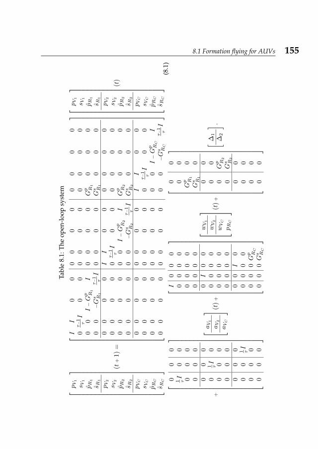
8.1 Formation flying for AUVs 155Ta
ble
8.1:
The
open
-loo
psy
stem
pV1
s V1
pR
1
s R1
pV2
s V2
pR
2
s R2
pVC
s VC
pRC
s RC
(t+
1)=
II
00
00
00
00
00
0τ−1τI
00
00
00
00
00
00
I−Gp R
1I
00
00
Gp R
10
00
00
−Gs R
1
τ−1τI
00
00
Gs R
10
00
00
00
II
00
00
00
00
00
0τ−1τI
00
00
00
00
00
00
I−Gp R
2I
Gp R
20
00
00
00
00
−Gs R
2
τ−1τI
Gs R
20
00
00
00
00
00
II
00
00
00
00
00
0τ−1τI
00
00
00
00
00
00
I−Gp RC
I0
00
00
00
00
0−Gs RC
τ−1τI
pV1
s V1
pR
1
s R1
pV2
s V2
pR
2
s R2
pVC
s VC
pRC
s RC
(t)
+
00
01 τI
00
00
00
00
00
00
1 τI
00
00
00
00
00
00
1 τI
00
00
00
aV1
aV2
aVC
(t)+
I0
00
00
00
00
00
00
00
0I
00
00
00
00
00
00
00
00
I0
00
00
00
0Gp RC
00
0Gs RC
wV1
wV2
wVC
pRC
(t)+
00
00
Gp R
10
Gs R
10
00
00
0Gp R
2
0Gs R
2
00
00
00
00
[ ∆1
∆2
] .
(8.1
)
156 Chapter 8: Case Studies
Possible solutions of the control problem are constrained by the fact that in prac-tice, the velocities and accelerations of all vehicles are bounded in norm. The po-sitions of the vehicles may also be constrained, e.g. by obstacles or if they shouldstay within a certain region. This will not be taken into account here.
The combined consideration of both control objectives and the constraintleads to a very difficult control problem. Finding an optimal control law (if oneexists) would involve on-line computations of a complexity that is not feasible forthe type of vehicles considered here (see [59]). Hence, our approach is to treat theobjectives and constraint one-by-one; this does not lead to an optimal control law,but to an admissible control law that performs well, and that can be implementedwith limited on-board computing power.
In the following, we start by solving the tracking problems for the vehicles,first for the setting with communication constraints, and then for the setting with-out communication constraints. We then augment the optimal control law foundfor the tracking problem in such a way that the bounds on the speed and accel-eration are achieved. Finally we consider the problems of stability and collision:In the case with communication constraints, we have to utilize the event-basedfeedback from V1 and V2 to VC in order to avoid collisions.
8.1.4.1 The tracking problem, with communication constraints
First we only look at the tracking problem, ignoring the collision problem andbounds. Each vehicle Vj tries to track its observed reference position, while avoid-ing excessive control efforts. The tracking problem for each vehicle Vj can beformulated as an LQ optimal control problem (see e.g. [63]):
minaVj
∞∑t=t0
∥∥pVj (t) − pRj (t)∥∥2+ α
∥∥aVj (t)∥∥2, j = 1, 2, C.
Here, α ∈ R is a parameter weighing the cost of acceleration against the cost ofdeviating from the reference trajectory.
The infinite-horizon formulation is chosen for simplicity, and all disturbancesare ignored for now, since otherwise and without discounting, the cost would beinfinite.
The difference vector[pVj − pRjsVj − sRj
]has dynamics
[pVj − pRjsVj − sRj
](t + 1) =
[I I0 τ−1
τ I
] [pVj − pRjsVj − sRj
](t)
+
[01τ I
]aVj (t) +
[I0
]wVj (t) +
[GpRjGsRj
](pRj − pRj )(t),
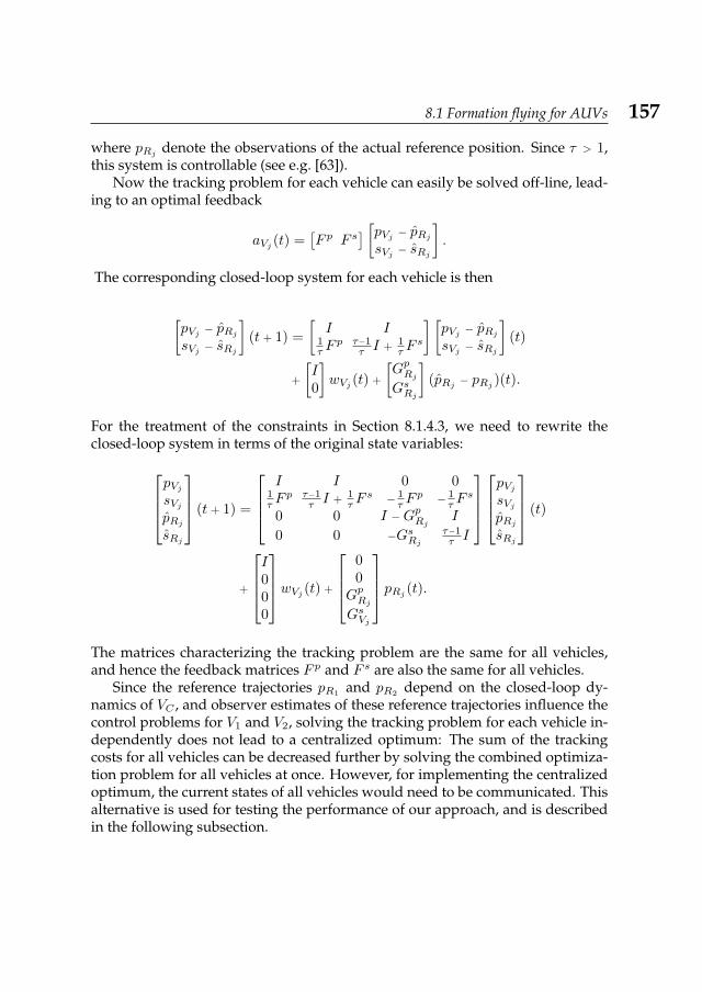
8.1 Formation flying for AUVs 157
where pRj denote the observations of the actual reference position. Since τ > 1,this system is controllable (see e.g. [63]).
Now the tracking problem for each vehicle can easily be solved off-line, lead-ing to an optimal feedback
aVj (t) =[F p F s
] [pVj − pRjsVj − sRj
].
The corresponding closed-loop system for each vehicle is then
[pVj − pRjsVj − sRj
](t + 1) =
[I I
1τ F
p τ−1τ I + 1
τ Fs
] [pVj − pRjsVj − sRj
](t)
+
[I0
]wVj (t) +
[GpRjGsRj
](pRj − pRj )(t).
For the treatment of the constraints in Section 8.1.4.3, we need to rewrite theclosed-loop system in terms of the original state variables:
pVjsVjpRjsRj
(t + 1) =
I I 0 0
1τ F
p τ−1τ I + 1
τ Fs − 1
τ Fp − 1
τ Fs
0 0 I −GpRj I
0 0 −GsRjτ−1τ I
pVjsVjpRjsRj
(t)
+
I000
wVj (t) +
00
GpRjGsVj
pRj (t).The matrices characterizing the tracking problem are the same for all vehicles,and hence the feedback matrices F p and F s are also the same for all vehicles.
Since the reference trajectories pR1 and pR2 depend on the closed-loop dy-namics of VC , and observer estimates of these reference trajectories influence thecontrol problems for V1 and V2, solving the tracking problem for each vehicle in-dependently does not lead to a centralized optimum: The sum of the trackingcosts for all vehicles can be decreased further by solving the combined optimiza-tion problem for all vehicles at once. However, for implementing the centralizedoptimum, the current states of all vehicles would need to be communicated. Thisalternative is used for testing the performance of our approach, and is describedin the following subsection.

158 Chapter 8: Case Studies
8.1.4.2 The tracking problem, without communication constraints
In this subsection, the same open-loop system for the motion of the vehicles isused. All communications are subject to the same uncertainties as in the settingwith communication constraints. However, in this setting we do not impose anyconstraints on the communication of the local state observations among the ve-hicles. We include this setting for comparison purposes – this will allow us toquantify the costs and benefits of communication in our simulation.
In this setting, each vehicle has observers for the states of all other vehicles, soin other words each vehicle keeps a copy of the whole system in memory, withexact values for its own state, and observers for the states of the other vehicles.The control feedback for the tracking problem is the same for all vehicles: Theyall solve the combined tracking problem
minaV1 ,aV2 ,aVC
∞∑t=t0
∥∥∥∥∥∥pV1(t) − pVC (t) −∆1
pV2(t) − pVC (t) −∆2
pVC (t) − pRC (t)
∥∥∥∥∥∥2
+ α
∥∥∥∥∥∥aV1(t)aV2(t)aVC (t)
∥∥∥∥∥∥2
.
The solution of this LQ-problem is
aV1
aV2
aVC
=
F11 F12 F13 F14 F15 F16
F21 F22 F23 F24 F25 F26
F31 F32 F33 F34 F35 F36
pV1
− pVC −∆1
sV1 − sVCpV2 − pVC −∆2
sV2− sVC
pVC − pRCsVC − sRC
,
where F11, . . . , F36 ∈ R3×3 can be found off-line.Each vehicle has its own copy of the overall closed-loop system, with observer
estimates for the states of the other vehicles.
8.1.4.3 The bounds on velocity and acceleration
Since the norm of the acceleration for each vehicle is penalized in the cost functionof the tracking problem, the accelerations found from the state feedbacks for thetwo settings above will usually be small in norm. However, this does not guaran-tee that they stay within fixed bounds. Moreover, the velocities of the vehicles arenot bounded as a result of the state feedbacks found above, and we might need afixed bound on the speed of each vehicle for a realistic model of the settings.
With upper bounds amax ∈ R and smax ∈ R on the acceleration and speed ofeach vehicle, we define λs ∈ R by
8.1 Formation flying for AUVs 159
λs =1
‖aVj‖2(
(1 − τ)aTVjsVj +
√(τ − 1)2aTVj (sVja
TVj− aVjs
TVj
)sVj + τ2s2max‖aVj‖2
).
This variable is used for limiting the speed of the vehicle, and is derived fromrequiring that the velocity sVj (t + 1) obtained by applying the corrected inputλsaVj (t) satisfies
‖sVj (t + 1)‖2 = ‖τ − 1
τsVj (t) +
1
τλsaVj (t)‖2 = s2
max.
A simple (but not necessarily optimal) way of implementing a fixed upper boundon the acceleration and speed of each vehicle is to use the following control input:
aVj (t) = min
λs,
amax
‖aVj (t)‖, 1
∗ aVj (t),
where aVj (t) is the optimal control feedback found in the previous two subsec-tions, depending on the setting. This control law satisfies the bounds ‖aVj (t)‖ ≤amax and ‖sVj (t + 1)‖ ≤ smax.
8.1.4.4 Stability and the collision constraint
In practice the speed and the acceleration of an AUV are bounded. This meansthat, even though both of the closed-loop systems derived in the previous sub-sections are output stable with respect to the output
y(t) =
pV1(t) − pVC (t) −∆1
pV2(t) − pVC (t) −∆2
pVC (t) − pRC (t)
,the closed-loop systems together with the constraints ‖a‖ ≤ amax and ‖s‖ ≤ smax
might not be output stable.This is interpreted as follows: If the external reference signal moves at a speed
higher than smax then VC is not able to track the reference signal, and pVC − pRCincreases. There is nothing that can be done about this. Another possibility is thatthe followers V1 and V2 cannot track their reference positions, because they aresubjected to strong disturbances and cannot accelerate enough to compensate forthat. This may lead to a follower being left behind, or a collision of two vehicles.This can be avoided if VC is informed about the positions of V1 and V2, at least inthe case that V1 or V2 are deviating too much from their reference positions. Forthis potential problem, we suggest three possible solutions:
160 Chapter 8: Case Studies
• VC receives feedback from V1 and V2 regularly, and includes these positionsinto its local tracking problem. The deviation from the formation will besmall, but this involves more communication than necessary.
• VC receives feedback from V1 or V2 only in the case that a follower vehicleis too far from its reference position, i.e. if ‖pVj − (pVC + ∆j)‖ ≥ r for somefixed r > 0. In this way, the communication from V1 and V2 to VC is keptminimal. If the safety regions of radius r around V1 and V2 are chosen farenough from each other then this approach avoids collision.
• We set the maximum speed of VC well below the actual maximum speedof V1 and V2. The follower vehicles have a better chance at tracking theirreference signal. No additional communication is necessary, however VCcannot fly at its maximum speed, and hence might have more difficultiestracking the external reference signal.
In this case study we choose the second option: At each time instant, the fol-lower vehicles check whether their position deviates from their observed refer-ence position by more than r. If that is the case, they send their position pVj toVC .
There are several possibilities for VC to use this information in order to helpthe follower vehicle get back into formation. One option, which turned out to besuccessful in simulations, is to have the VC track the signal
pRC +(pV1 −∆1 − pVC )I1 + (pV2 −∆2 − pVC )I2
W
instead of the signal pRC , where Ij = 1 if VC received pVj from Vj during thistime step, and Ij = 0 otherwise. The second term is a weighted average of thedeviations of the vehicle positions from their reference positions, with weight pa-rameterW > 0. This average deviation has to be computed by VC . At most times,VC does not know the positions of the follower vehicles because the follower ve-hicles are within a radius r of their reference positions. In this case, the trackingsignal is pRC .
The collision problem is automatically solved by our approach if the distancebetween the uncertainty regions Dr(pVj ) for the two follower vehicles is largeenough - this can be made more precise by taking into account the maximumspeed and acceleration.
8.1.4.5 The control algorithm
We summarize the control algorithm described in the previous subsections:For the case with communication constraints, we have
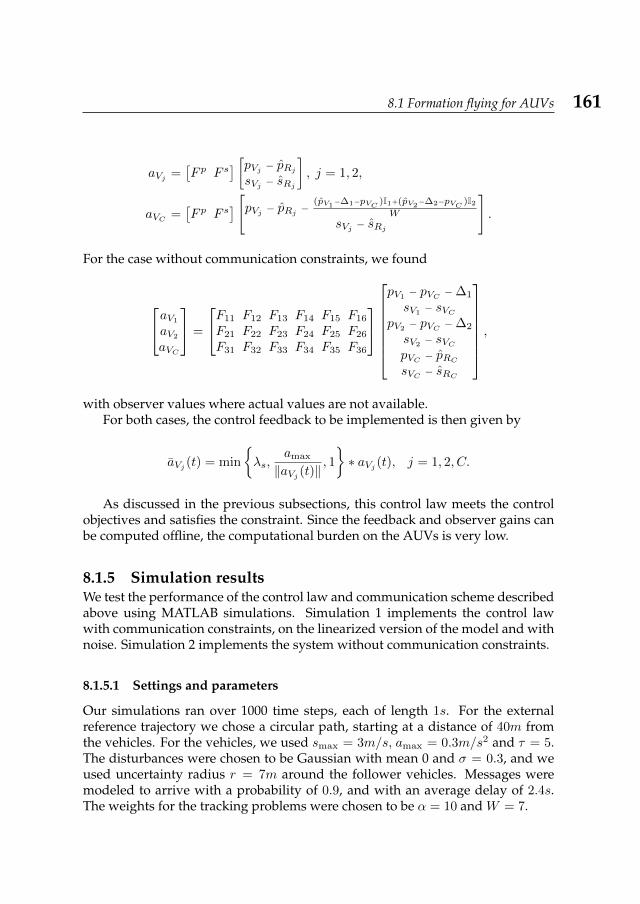
8.1 Formation flying for AUVs 161
aVj =[F p F s
] [pVj − pRjsVj − sRj
], j = 1, 2,
aVC =[F p F s
] [pVj − pRj − (pV1−∆1−pVC )I1+(pV2−∆2−pVC )I2W
sVj − sRj
].
For the case without communication constraints, we found
aV1
aV2
aVC
=
F11 F12 F13 F14 F15 F16
F21 F22 F23 F24 F25 F26
F31 F32 F33 F34 F35 F36
pV1
− pVC −∆1
sV1− sVC
pV2− pVC −∆2
sV2− sVC
pVC − pRCsVC − sRC
,
with observer values where actual values are not available.For both cases, the control feedback to be implemented is then given by
aVj (t) = min
λs,
amax
‖aVj (t)‖, 1
∗ aVj (t), j = 1, 2, C.
As discussed in the previous subsections, this control law meets the controlobjectives and satisfies the constraint. Since the feedback and observer gains canbe computed offline, the computational burden on the AUVs is very low.
8.1.5 Simulation resultsWe test the performance of the control law and communication scheme describedabove using MATLAB simulations. Simulation 1 implements the control lawwith communication constraints, on the linearized version of the model and withnoise. Simulation 2 implements the system without communication constraints.
8.1.5.1 Settings and parameters
Our simulations ran over 1000 time steps, each of length 1s. For the externalreference trajectory we chose a circular path, starting at a distance of 40m fromthe vehicles. For the vehicles, we used smax = 3m/s, amax = 0.3m/s2 and τ = 5.The disturbances were chosen to be Gaussian with mean 0 and σ = 0.3, and weused uncertainty radius r = 7m around the follower vehicles. Messages weremodeled to arrive with a probability of 0.9, and with an average delay of 2.4s.The weights for the tracking problems were chosen to be α = 10 and W = 7.
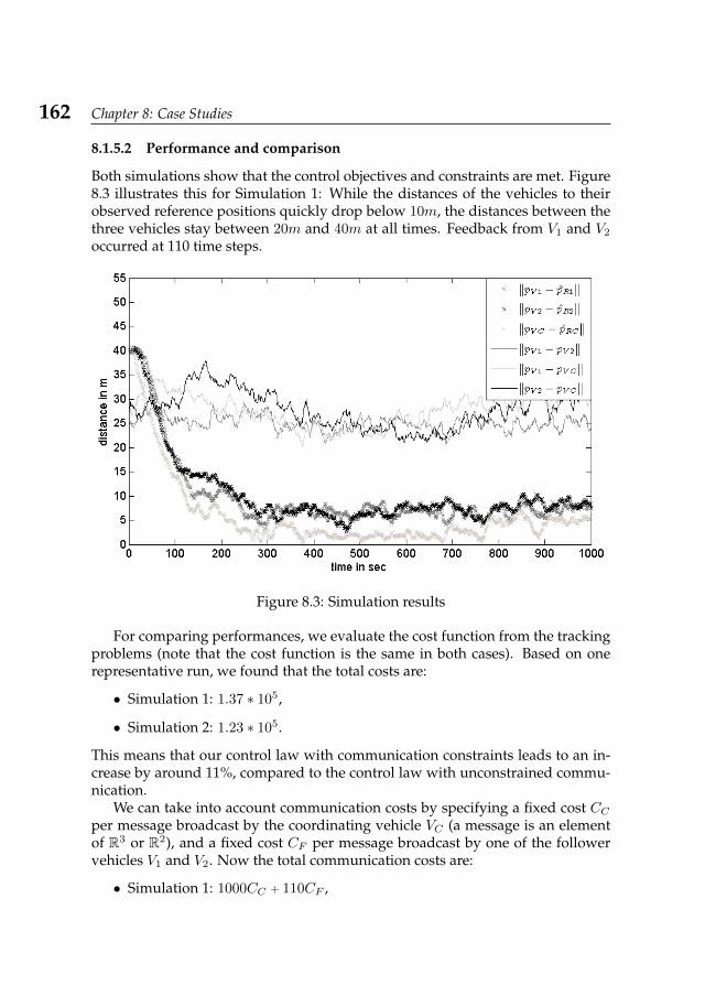
162 Chapter 8: Case Studies
8.1.5.2 Performance and comparison
Both simulations show that the control objectives and constraints are met. Figure8.3 illustrates this for Simulation 1: While the distances of the vehicles to theirobserved reference positions quickly drop below 10m, the distances between thethree vehicles stay between 20m and 40m at all times. Feedback from V1 and V2
occurred at 110 time steps.
Figure 8.3: Simulation results
For comparing performances, we evaluate the cost function from the trackingproblems (note that the cost function is the same in both cases). Based on onerepresentative run, we found that the total costs are:
• Simulation 1: 1.37 ∗ 105,
• Simulation 2: 1.23 ∗ 105.
This means that our control law with communication constraints leads to an in-crease by around 11%, compared to the control law with unconstrained commu-nication.
We can take into account communication costs by specifying a fixed cost CCper message broadcast by the coordinating vehicle VC (a message is an elementof R3 or R2), and a fixed cost CF per message broadcast by one of the followervehicles V1 and V2. Now the total communication costs are:
• Simulation 1: 1000CC + 110CF ,
8.2 Coordinated ramp metering 163
• Simulation 2: 2000CC + 2000CF .
The communication costs for Simulation 1 depend strongly on the disturbances,and on the radius r of the uncertainty regions.
8.1.6 Concluding remarksIn this section, we described a control algorithm and a communication scheme forthe problem of formation flying for AUVs. This approach is implementable withlow on-board computing power, and it requires very little communication amongthe vehicles. In a simulation, we compared the performances of this approach anda similar approach with unlimited communication. While the total cost increasedslightly with our communication scheme, the total amount of communicationdecreased considerably.
Another case study was worked out for the problem of collision avoidancefor several unmanned aerial vehicles, coordinated by a control tower. Since theapproaches and results are very similar to the case study discussed in this section,the case study for unmanned aerial vehicles is not included here.
8.2 Coordinated ramp meteringThis section describes an application of coordination control, concerning the co-ordinated control of several ramp metering devices at highway on-ramps.
8.2.1 IntroductionRamp metering devices are traffic lights at the on-ramps of a highway, which al-low one vehicle to get onto the highway every s seconds, where s ∈ [0,∞) can bechosen by the controller (i.e. the road authorities). Ramp metering is employedin order to achieve two control objectives: flow control and temporization. Flowcontrol concerns the regulation of the on-flow onto the highway in the case thatthe overall demand exceeds the highway capacity: it is used to avoid traffic jamson the highway, at the expense of creating queues at the on-ramp. The rationalebehind this choice is based on a hierarchical ordering of – possibly conflicting –control objectives: If the overall traffic in a network exceeds the overall capacity,queues cannot be avoided. Our first priority in that case is to keep the largestroads, the highways, queue-free, at the expense of the smaller roads. Temporiza-tion is a process which ‘evens out’ the traffic flow: In the city network, vehiclestypically move in batches (or platoons) from intersection to intersection. By let-ting vehicles onto the highway at equally-spaced time points, the ramp meteringdevice removes this effect, thus reducing the variance of the traffic flow on thehighway. In the following, we will only consider the objective of flow control.
164 Chapter 8: Case Studies
The need for coordination of different ramp metering devices arises when sev-eral neighboring on-ramps, leading vehicles onto the same direction of the high-way, have a combined demand exceeding the downstream capacity of the high-way – in that case, local control would lead to long queues at the downstreamon-ramps since the upstream on-ramps ignore downstream demand when deter-mining their on-flow2.
Coordination schemes for ramp metering were first implemented in Los An-geles and Delft. Later, research on coordinated ramp metering has focused on thehighway rings of Amsterdam and Paris, for which historical traffic data is avail-able. The highway traffic on the Amsterdam ring is currently monitored and con-trolled from the traffic control center of North-Holland. In [30, 42], a centralizedapproach (i.e. all on-ramp flows are determined by the traffic control center) tocoordinated ramp metering was tested on several non-linear traffic models, andapplied in simulations to the highway rings of Amsterdam and Paris. The controlobjectives were to minimize the total time spent by all drivers in the network, andto have equal queue lengths at the on-ramps. The centralized approach used wascomputationally feasible for the simulation studies3, but did not necessarily leadto a global optimum.
A decentralized approach to coordinated ramp metering was suggested in[73–75], and applied in simulations to the Amsterdam ring: Each on-ramp used alocal controller, and only when its local maximum queue length was exceeded, itwould tell the next upstream on-ramp to reduce its on-flow accordingly. Duringpeak hours, this coordination process would then naturally propagate upstream.This approach has the advantage of high scalability, but does not perform well inall situations (e.g. if there is no demand at the next upstream on-ramp).
In the following, we will apply the concepts of coordination control derived inearlier chapters to this problem, using a simple linear traffic model. The purposeof this section is to illustrate the theory of coordinated linear systems, but alsoto give some insight into the separation of this problem into global and localsubproblems.
8.2.2 ModelingFor the purpose of this case study, we use a strongly simplified linear version ofthe traffic model found in [66]. In particular, we make the following modelingassumptions:
• the speed is constant for all vehicles and at all times,
• we restrict attention to two neighboring on-ramps,
2In urban areas, this can lead to vehicles driving back to the next upstream on-ramp via the citynetwork – a detour on their part, and an unnecessary load on city traffic.
3Extendability is of course limited in the centralized approach – a national highway network maybe too large.
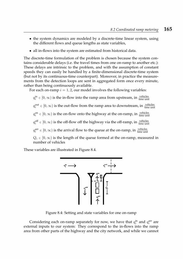
8.2 Coordinated ramp metering 165
• the system dynamics are modeled by a discrete-time linear system, usingthe different flows and queue lengths as state variables,
• all in-flows into the system are estimated from historical data.
The discrete-time formulation of the problem is chosen because the system con-tains considerable delays (i.e. the travel times from one on-ramp to another etc.):These delays are intrinsic to the problem, and with the assumption of constantspeeds they can easily be handled by a finite-dimensional discrete-time system(but not by its continuous-time counterpart). Moreover, in practice the measure-ments from the detection loops are sent in aggregated form once every minute,rather than being continuously available.
For each on-ramp i = 1, 2, our model involves the following variables:
qini ∈ [0,∞) is the in-flow into the ramp area from upstream, in vehicles
time unit
qouti ∈ [0,∞) is the out-flow from the ramp area to downstream, in vehicles
time unit
qoni ∈ [0,∞) is the on-flow onto the highway at the on-ramp, in vehicles
time unit
qoffi ∈ [0,∞) is the off-flow off the highway via the off-ramp, in vehicles
time unit
qarri ∈ [0,∞) is the arrival flow to the queue at the on-ramp, in vehicles
time unit
Qi ∈ [0,∞) is the length of the queue formed at the on-ramp, measured innumber of vehicles
These variables are illustrated in Figure 8.4.
Figure 8.4: Setting and state variables for one on-ramp
Considering each on-ramp separately for now, we have that qini and qarr
i areexternal inputs to our system: They correspond to the in-flows into the ramparea from other parts of the highway and the city network, and while we cannot
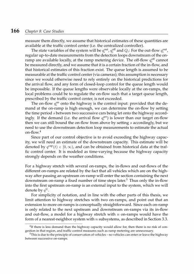
166 Chapter 8: Case Studies
measure them directly, we assume that historical estimates of these quantities areavailable at the traffic control center (i.e. the centralized controller).
The state variables of the system will be qouti , qoff
i and Qi: For the out-flow qouti ,
regular up-to-date measurements from the detection loops downstream of the on-ramp are available locally, at the ramp metering device. The off-flow qoff
i cannotbe measured directly, and we assume that it is a certain fraction of the in-flow, andthat historical estimates of this fraction exist. The queue length is assumed to bemeasurable at the traffic control center (via cameras); this assumption is necessarysince we would otherwise need to rely entirely on the historical predictions forthe arrival flow, and any form of closed-loop control for the queue length wouldbe impossible. If the queue lengths were observable locally at the on-ramps, thelocal problems could be to regulate the on-flow such that a target queue length,prescribed by the traffic control center, is not exceeded.
The on-flow qoni onto the highway is the control input: provided that the de-
mand at the on-ramp is high enough, we can determine the on-flow by settingthe time period s between two successive cars being let onto the highway accord-ingly. If the demand (i.e. the arrival flow qarr
i ) is lower than our target on-flowthen we can still bound the on-flow from above by setting s accordingly, but weneed to use the downstream detection loop measurements to estimate the actualon-flow.4
Since part of our control objective is to avoid exceeding the highway capac-ity, we will need an estimate of the downstream capacity. This estimate will bedenoted by qcap(t) ∈ [0,∞), and can be obtained from historical data at the traf-fic control center. It is modeled as time-varying because the highway capacitystrongly depends on the weather conditions.
For a highway stretch with several on-ramps, the in-flows and out-flows of thedifferent on-ramps are related by the fact that all vehicles which are on the high-way after passing an upstream on-ramp will enter the section containing the nextdownstream on-ramp a fixed number of time steps later.5 Thus only the in-flowinto the first upstream on-ramp is an external input to the system, which we willdenote by qU.
For simplicity of notation, and in line with the other parts of this thesis, welimit attention to highway stretches with two on-ramps, and point out that anextension to more on-ramps is conceptually straightforward. Since each on-rampis only related to the next upstream and downstream on-ramps via its in-flowand out-flow, a model for a highway stretch with n on-ramps would have theform of a nearest-neighbor system with n subsystems, as described in Section 3.3.
4If there is less demand than the highway capacity would allow for, then there is no risk of con-gestion in that region, and traffic control measures such as ramp metering are unnecessary.
5This is due to the principle of conservation of vehicles – no vehicles can enter or leave the highwaybetween successive on-ramps.
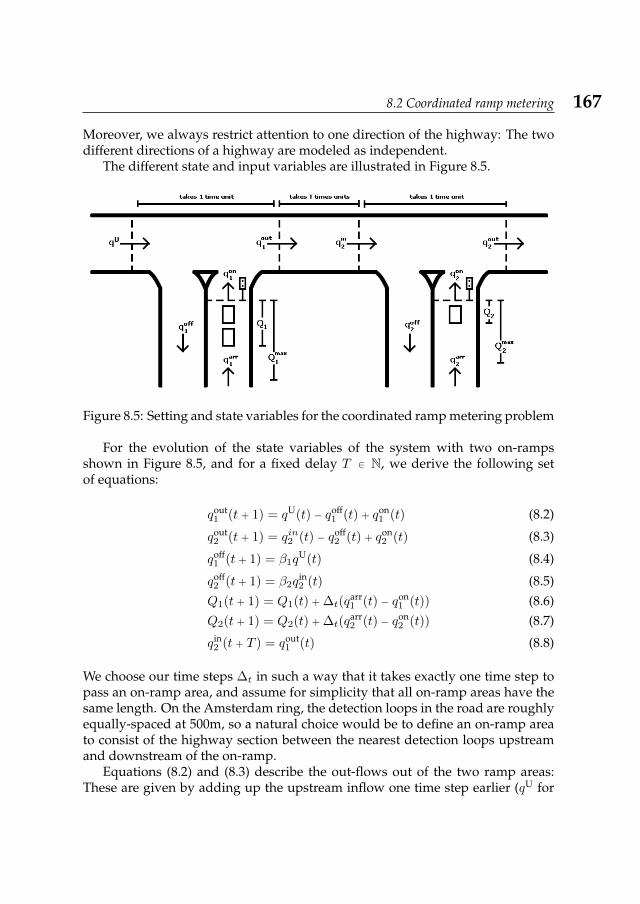
8.2 Coordinated ramp metering 167
Moreover, we always restrict attention to one direction of the highway: The twodifferent directions of a highway are modeled as independent.
The different state and input variables are illustrated in Figure 8.5.
Figure 8.5: Setting and state variables for the coordinated ramp metering problem
For the evolution of the state variables of the system with two on-rampsshown in Figure 8.5, and for a fixed delay T ∈ N, we derive the following setof equations:
qout1 (t + 1) = qU(t) − qoff
1 (t) + qon1 (t) (8.2)
qout2 (t + 1) = qin2 (t) − qoff
2 (t) + qon2 (t) (8.3)
qoff1 (t + 1) = β1q
U(t) (8.4)
qoff2 (t + 1) = β2q
in2 (t) (8.5)
Q1(t + 1) = Q1(t) + ∆t(qarr1 (t) − qon
1 (t)) (8.6)Q2(t + 1) = Q2(t) + ∆t(q
arr2 (t) − qon
2 (t)) (8.7)
qin2 (t + T ) = qout
1 (t) (8.8)
We choose our time steps ∆t in such a way that it takes exactly one time step topass an on-ramp area, and assume for simplicity that all on-ramp areas have thesame length. On the Amsterdam ring, the detection loops in the road are roughlyequally-spaced at 500m, so a natural choice would be to define an on-ramp areato consist of the highway section between the nearest detection loops upstreamand downstream of the on-ramp.
Equations (8.2) and (8.3) describe the out-flows out of the two ramp areas:These are given by adding up the upstream inflow one time step earlier (qU for
168 Chapter 8: Case Studies
ramp 1 and qin2 for ramp 2) and the on-flow via the respective on-ramp (qon
i ), anddeducting the off-flow at the respective off-ramp (qoff
i ).The off-flows qoff
1 and qoff2 are modeled as fixed fractions of the in-flows into
the respective ramp areas. The parameters β1, β2 ∈ [0,∞) appearing in equations(8.4) and (8.5) were assumed to be estimated from historical data; they are treatedas time-invariant in our setting, but may in principle be slowly time-varying (e.g.they may differ for the morning and evening rush hours).
In equations (8.6) and (8.7), the queue lengths at the two ramp metering de-vices are described to grow by the number of new vehicles arriving at the on-ramp over one time step, and to shrink by the number of vehicles which were letonto the highway by the ramp metering device over the same time period. Since∆t is the length of one time step, these two quantities can easily be estimated by∆tq
arr1 (t) and ∆tq
on2 (t). Note that these equations do not account for the fact that
queue lengths can never be negative in practice – again we justify this choice byarguing that if the demand is far below the highway capacity then there is no riskof congestion, and the ramp metering device does not need to restrict the on-flow.
Equation (8.8) models the interconnection between the two on-ramps, as de-scribed above: Under the assumption of constant speed, the out-flow out of ramparea 1 will reach ramp area 2 T time units later. Incorporating equation (8.8) intoour system requires us to keep the last T − 1 values for qin
2 in memory: SupposeT = 3, then the equation can be rewritten in the form
qin,+22
qin,+12
qin2
(t + 1) =
0 0 01 0 00 1 0
qin,+22
qin,+12
qin2
(t) +
100
qout1 (t), (8.9)
with auxiliary variables qin,+22 and qin,+1
2 satisfying
qin,+22 (t) = qin
2 (t + 2) and qin,+12 (t) = qin
2 (t + 1).
Combining equations (8.2)-(8.8) and (8.9), and re-ordering the state and inputvariables according to their locations (i.e. ramp 1 or ramp 2), we arrive at theopen-loop system given in Table 8.2.2. This system is a nearest-neighbor systemwith a directed information structure, or equivalently, a hierarchical system witha chain structure. In order to incorporate in the model which state variable is
observable from which location, we define an output vector
y1
y2
yc
, where yi con-
sists of all variables which are observable at ramp i (i = 1, 2), and yc contains allobservations available at the traffic control center.
8.2 Coordinated ramp metering 169
qout1
qoff1
Q1
qin,+22
qin,+12
qin2
qout2
qoff2
Q2
(t + 1) =
0 −1 0 0 0 0 0 0 00 0 0 0 0 0 0 0 00 0 1 0 0 0 0 0 01 0 0 0 0 0 0 0 00 0 0 1 0 0 0 0 00 0 0 0 1 0 0 0 00 0 0 0 0 1 0 −1 00 0 0 0 0 β2 0 0 00 0 0 0 0 0 0 0 1
qout1
qoff1
Q1
qin,+22
qin,+12
qin2
qout2
qoff2
Q2
(t)
+
1 0 0 0β1 0 0 00 ∆t 0 00 0 0 00 0 0 00 0 0 00 0 0 00 0 0 00 0 ∆t 0
qU
qarr1
qarr2
qcap
(t) +
1 00 0−∆t 0
0 00 00 00 10 00 −∆t
[qon1
qon2
](t)
(8.10)
Table 8.2: The open-loop system, for two on-ramps
We arrive at the output equation
y1
y2
yc,1yc,2yc,3yc,4yc,5yc,6
=
1 0 0 0 0 0 0 0 00 0 0 0 0 0 1 0 00 0 1 0 0 0 0 0 00 0 0 0 0 0 0 0 10 0 0 0 0 0 0 0 00 0 0 0 0 0 0 0 00 0 0 0 0 0 0 0 00 0 0 0 0 0 0 0 0
qout1
qoff1
Q1
qin,+22
qin,+12
qin2
qout2
qoff2
Q2
+
0 0 0 00 0 0 00 0 0 00 0 0 01 0 0 00 1 0 00 0 1 00 0 0 1
qU
qarr1
qarr2
qcap
.
8.2.3 Control problemAs already mentioned above, our control objective will be to have equal queuelengths while ensuring that the downstream flow does not exceed the highwaycapacity. In the following we justify this choice, discuss possible ways of for-malizing this objective, and split the overall objective into local control problems
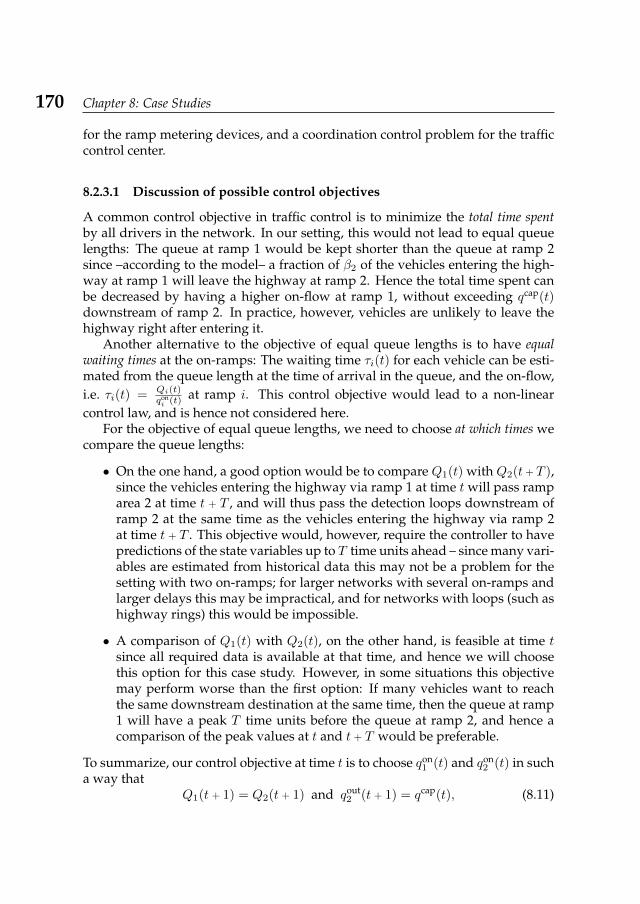
170 Chapter 8: Case Studies
for the ramp metering devices, and a coordination control problem for the trafficcontrol center.
8.2.3.1 Discussion of possible control objectives
A common control objective in traffic control is to minimize the total time spentby all drivers in the network. In our setting, this would not lead to equal queuelengths: The queue at ramp 1 would be kept shorter than the queue at ramp 2since –according to the model– a fraction of β2 of the vehicles entering the high-way at ramp 1 will leave the highway at ramp 2. Hence the total time spent canbe decreased by having a higher on-flow at ramp 1, without exceeding qcap(t)downstream of ramp 2. In practice, however, vehicles are unlikely to leave thehighway right after entering it.
Another alternative to the objective of equal queue lengths is to have equalwaiting times at the on-ramps: The waiting time τi(t) for each vehicle can be esti-mated from the queue length at the time of arrival in the queue, and the on-flow,i.e. τi(t) = Qi(t)
qoni (t) at ramp i. This control objective would lead to a non-linear
control law, and is hence not considered here.For the objective of equal queue lengths, we need to choose at which times we
compare the queue lengths:
• On the one hand, a good option would be to compare Q1(t) with Q2(t + T ),since the vehicles entering the highway via ramp 1 at time t will pass ramparea 2 at time t + T , and will thus pass the detection loops downstream oframp 2 at the same time as the vehicles entering the highway via ramp 2at time t + T . This objective would, however, require the controller to havepredictions of the state variables up to T time units ahead – since many vari-ables are estimated from historical data this may not be a problem for thesetting with two on-ramps; for larger networks with several on-ramps andlarger delays this may be impractical, and for networks with loops (such ashighway rings) this would be impossible.
• A comparison of Q1(t) with Q2(t), on the other hand, is feasible at time tsince all required data is available at that time, and hence we will choosethis option for this case study. However, in some situations this objectivemay perform worse than the first option: If many vehicles want to reachthe same downstream destination at the same time, then the queue at ramp1 will have a peak T time units before the queue at ramp 2, and hence acomparison of the peak values at t and t + T would be preferable.
To summarize, our control objective at time t is to choose qon1 (t) and qon
2 (t) in sucha way that
Q1(t + 1) = Q2(t + 1) and qout2 (t + 1) = qcap(t), (8.11)
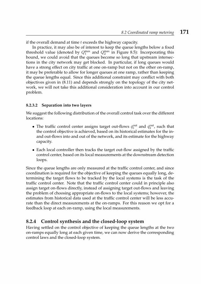
8.2 Coordinated ramp metering 171
if the overall demand at time t exceeds the highway capacity.In practice, it may also be of interest to keep the queue lengths below a fixed
threshold value (denoted by Qmax1 and Qmax
2 in Figure 8.5): Incorporating thisbound, we could avoid that the queues become so long that upstream intersec-tions in the city network may get blocked. In particular, if long queues wouldhave a strong effect on city traffic at one on-ramp but not on the other on-ramp,it may be preferable to allow for longer queues at one ramp, rather than keepingthe queue lengths equal. Since this additional constraint may conflict with bothobjectives given in (8.11) and depends strongly on the topology of the city net-work, we will not take this additional consideration into account in our controlproblem.
8.2.3.2 Separation into two layers
We suggest the following distribution of the overall control task over the differentlocations:
• The traffic control center assigns target out-flows qout1 and qout
2 , such thatthe control objective is achieved, based on its historical estimates for the in-and out-flows into and out of the network, and its estimate for the highwaycapacity.
• Each local controller then tracks the target out-flow assigned by the trafficcontrol center, based on its local measurements at the downstream detectionloops.
Since the queue lengths are only measured at the traffic control center, and sincecoordination is required for the objective of keeping the queues equally long, de-termining the target flows to be tracked by the local systems is the task of thetraffic control center. Note that the traffic control center could in principle alsoassign target on-flows directly, instead of assigning target out-flows and leavingthe problem of choosing appropriate on-flows to the local systems; however, theestimates from historical data used at the traffic control center will be less accu-rate than the direct measurements at the on-ramps. For this reason we opt for afeedback loop at each on-ramp, using the local measurements.
8.2.4 Control synthesis and the closed-loop systemHaving settled on the control objective of keeping the queue lengths at the twoon-ramps equally long at each given time, we can now derive the correspondingcontrol laws and the closed-loop system.
172 Chapter 8: Case Studies
8.2.4.1 Control law for the coordinator
The target out-flows qout1 and qout
2 to be determined by the traffic control centercan be derived directly from the objectives given in (8.11). The variables whichare observable at the traffic control center are illustrated in Figure 8.6. We get
Figure 8.6: Variables observable at the traffic control center
qout2 (t + 1) = qcap(t), and qout
1 (t + 1) can be derived from the objective Q1(t + 1) =Q2(t + 1), using the system dynamics: Noting that
qoni (t) = qout
i (t + 1) − qini (t) + qoff
i (t) = qouti (t + 1) − (1 − βi)q
ini (t)
and qin2 (t) = qout
1 (t − T ), we get
Q1(t + 1) = Q2(t + 1)
⇔ Q1(t) + ∆t (qarr1 (t) − qon
1 (t)) = Q2(t) + ∆t (qarr2 (t) − qon
2 (t))
⇔ Q1(t) + ∆t
(qarr1 (t) − qout
1 (t + 1) + (1 − β1)qin1 (t)
)= Q2(t) + ∆t
(qarr2 (t) − qout
2 (t + 1) + (1 − β2)qin2 (t)
)⇔ qout
1 (t + 1) =1
∆t(Q1(t) −Q2(t)) + (qarr
1 (t) − qarr2 (t)) + (1 − β1)qU (t)
− (1 − β2)qout1 (t − T ) + qcap(t).
Implementing this control law will require us to keep the last T target out-flowsqout1 in memory. The control law for the traffic control center can be rewritten as
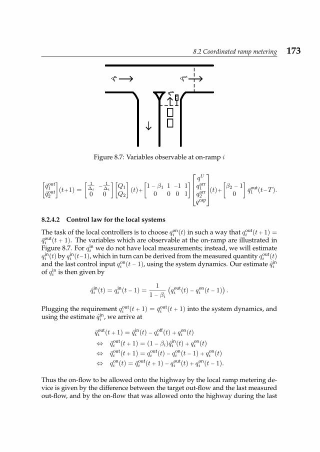
8.2 Coordinated ramp metering 173
Figure 8.7: Variables observable at on-ramp i
[qout1
qout2
](t+1) =
[1
∆t− 1
∆t
0 0
][Q1
Q2
](t)+
[1 − β1 1 −1 1
0 0 0 1
]qU
qarr1
qarr2
qcap
(t)+
[β2 − 1
0
]qout1 (t−T ).
8.2.4.2 Control law for the local systems
The task of the local controllers is to choose qoni (t) in such a way that qout
i (t + 1) =qouti (t + 1). The variables which are observable at the on-ramp are illustrated in
Figure 8.7. For qini we do not have local measurements; instead, we will estimate
qini (t) by qin
i (t−1), which in turn can be derived from the measured quantity qouti (t)
and the last control input qoni (t − 1), using the system dynamics. Our estimate qin
i
of qini is then given by
qini (t) = qin
i (t − 1) =1
1 − βi
(qouti (t) − qon
i (t − 1)).
Plugging the requirement qouti (t + 1) = qout
i (t + 1) into the system dynamics, andusing the estimate qin
i , we arrive at
qouti (t + 1) = qin
i (t) − qoffi (t) + qon
i (t)
⇔ qouti (t + 1) = (1 − βi)q
ini (t) + qon
i (t)
⇔ qouti (t + 1) = qout
i (t) − qoni (t − 1) + qon
i (t)
⇔ qoni (t) = qout
i (t + 1) − qouti (t) + qon
i (t − 1).
Thus the on-flow to be allowed onto the highway by the local ramp metering de-vice is given by the difference between the target out-flow and the last measuredout-flow, and by the on-flow that was allowed onto the highway during the last
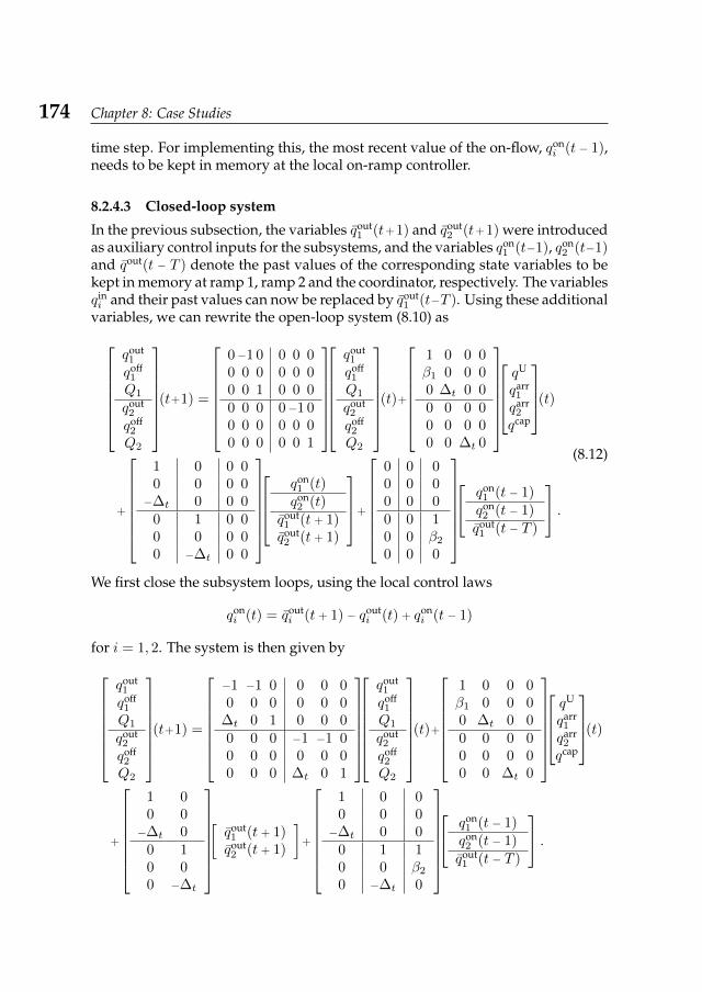
174 Chapter 8: Case Studies
time step. For implementing this, the most recent value of the on-flow, qoni (t − 1),
needs to be kept in memory at the local on-ramp controller.
8.2.4.3 Closed-loop system
In the previous subsection, the variables qout1 (t+1) and qout
2 (t+1) were introducedas auxiliary control inputs for the subsystems, and the variables qon
1 (t−1), qon2 (t−1)
and qout(t − T ) denote the past values of the corresponding state variables to bekept in memory at ramp 1, ramp 2 and the coordinator, respectively. The variablesqini and their past values can now be replaced by qout
1 (t−T ). Using these additionalvariables, we can rewrite the open-loop system (8.10) as
qout1
qoff1
Q1
qout2
qoff2
Q2
(t+1) =
0−1 0 0 0 00 0 0 0 0 00 0 1 0 0 00 0 0 0−1 00 0 0 0 0 00 0 0 0 0 1
qout1
qoff1
Q1
qout2
qoff2
Q2
(t)+
1 0 0 0β1 0 0 00 ∆t 0 00 0 0 00 0 0 00 0 ∆t 0
qU
qarr1
qarr2
qcap
(t)
+
1 0 0 00 0 0 0−∆t 0 0 0
0 1 0 00 0 0 00 −∆t 0 0
qon1 (t)qon2 (t)
qout1 (t + 1)qout2 (t + 1)
+
0 0 00 0 00 0 00 0 10 0 β2
0 0 0
qon
1 (t − 1)qon2 (t − 1)
qout1 (t − T )
.(8.12)
We first close the subsystem loops, using the local control laws
qoni (t) = qout
i (t + 1) − qouti (t) + qon
i (t − 1)
for i = 1, 2. The system is then given byqout1
qoff1
Q1
qout2
qoff2
Q2
(t+1) =
−1 −1 0 0 0 00 0 0 0 0 0
∆t 0 1 0 0 00 0 0 −1 −1 00 0 0 0 0 00 0 0 ∆t 0 1
qout1
qoff1
Q1
qout2
qoff2
Q2
(t)+
1 0 0 0β1 0 0 00 ∆t 0 00 0 0 00 0 0 00 0 ∆t 0
qU
qarr1
qarr2
qcap
(t)
+
1 00 0−∆t 0
0 10 00 −∆t
[qout1 (t + 1)qout2 (t + 1)
]+
1 0 00 0 0−∆t 0 0
0 1 10 0 β2
0 −∆t 0
qon
1 (t − 1)qon2 (t − 1)
qout1 (t − T )
.
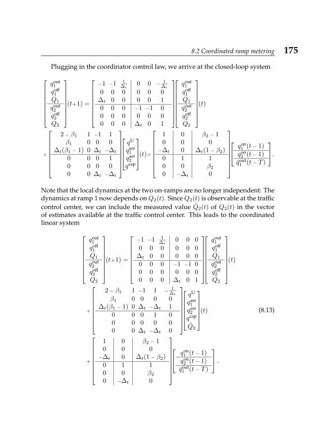
8.2 Coordinated ramp metering 175
Plugging in the coordinator control law, we arrive at the closed-loop systemqout1
qoff1
Q1
qout2
qoff2
Q2
(t+1) =
−1 −1 1
∆t0 0 − 1
∆t
0 0 0 0 0 0∆t 0 0 0 0 10 0 0 −1 −1 00 0 0 0 0 00 0 0 ∆t 0 1
qout1
qoff1
Q1
qout2
qoff2
Q2
(t)
+
2 − β1 1 −1 1β1 0 0 0
∆t(β1 − 1) 0 ∆t −∆t
0 0 0 10 0 0 00 0 ∆t −∆t
qU
qarr1
qarr2
qcap
(t)+
1 0 β2 − 10 0 0−∆t 0 ∆t(1 − β2)
0 1 10 0 β2
0 −∆t 0
qon
1 (t − 1)qon2 (t − 1)
qout1 (t − T )
.
Note that the local dynamics at the two on-ramps are no longer independent: Thedynamics at ramp 1 now depends onQ2(t). SinceQ2(t) is observable at the trafficcontrol center, we can include the measured value Q2(t) of Q2(t) in the vectorof estimates available at the traffic control center. This leads to the coordinatedlinear system
qout1
qoff1
Q1
qout2
qoff2
Q2
(t+1) =
−1 −1 1
∆t0 0 0
0 0 0 0 0 0∆t 0 0 0 0 00 0 0 −1 −1 00 0 0 0 0 00 0 0 ∆t 0 1
qout1
qoff1
Q1
qout2
qoff2
Q2
(t)
+
2 − β1 1 −1 1 − 1
∆t
β1 0 0 0 0∆t(β1 − 1) 0 ∆t −∆t 1
0 0 0 1 00 0 0 0 00 0 ∆t −∆t 0
qU
qarr1
qarr2
qcap
Q2
(t)
+
1 0 β2 − 10 0 0−∆t 0 ∆t(1 − β2)
0 1 10 0 β2
0 −∆t 0
qon
1 (t − 1)qon2 (t − 1)
qout1 (t − T )
.
(8.13)
176 Chapter 8: Case Studies
8.2.5 Concluding remarksIn this section, we motivated and discussed a coordinated ramp metering prob-lem. The traffic flows and queue lengths in the on-ramp areas were modeled as alinear system, and the control objective was discussed and formalized.
Whether the control objective can be achieved in a decentralized manner de-pends on which partial observations are available at which locations. For onepossible setting, we derived a suitable coordination control law and the corre-sponding closed-loop system.
Concluding Remarks 9In this concluding chapter, we briefly summarize the main contributions of thisthesis, and discuss several possible extensions.
9.1 Summary of the main resultsOne of the main contributions of this thesis is the derivation of explicit proce-dures for the transformation of interconnected or monolithic linear systems intocoordinated linear systems in Chapter 4: Finding appropriate system decompo-sitions if no a priori decomposition is given (as in the monolithic case) or thegiven decomposition is unsuitable for control purposes (as in the interconnectedcase) is a major problem in decentralized control. Three concepts of minimality ofdecompositions were introduced in order to identify decompositions which are‘as decentralized as possible’, and many of our decomposition procedures wereshown to produce such minimal decompositions.
Another relevant contribution to decentralized control theory is the refine-ment of the standard concepts of reachability and indistinguishability to reflectwhich input/output is used, and which part of the system is affected, and the sub-sequent distinction between jointly and independently reachable subspaces, andbetween completely and independently indistinguishable subspaces in Chapter5. These concepts helped us identify and characterize concepts of controllabilityand observability which are more meaningful for coordination control than thecorresponding standard concepts for monolithic systems.
The main result of this thesis is Theorem 6.2.7, together with its immediateconsequences for coordinated and hierarchical linear systems: When restrict-ing the set of admissible control laws for an LQ control problem to structure-preserving static state feedback, the optimal feedback for each subsystem onlydepends on the subsystem itself, and on its followers, but not on the rest of thehierarchy. This result allows us to approach the problem in a bottom-to-top man-ner, finding the optimal feedback for each subsystem numerically, at each stepusing an algorithm derived from Theorem 6.2.7 and the optimal feedbacks foundfor its follower systems in previous steps.
Finally, this control synthesis procedure for LQ control problems is adjustedto allow for event-based bottom-to-top feedback and to significantly reduce itscomputational complexity, in Chapter 7. The cost corresponding to this controllaw approximates the centralized optimum arbitrarily well, at the expense of anincreased need for bottom-to-top feedback.
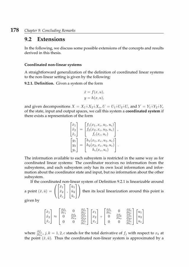
178 Chapter 9: Concluding Remarks
9.2 ExtensionsIn the following, we discuss some possible extensions of the concepts and resultsderived in this thesis.
Coordinated non-linear systems
A straightforward generalization of the definition of coordinated linear systemsto the non-linear setting is given by the following:
9.2.1. Definition. Given a system of the form
x = f(x, u),
y = h(x, u),
and given decompositions X = X1+X2+Xc, U = U1+U2+Uc and Y = Y1+Y2+Ycof the state, input and output spaces, we call this system a coordinated system ifthere exists a representation of the formx1
x2
xc
=
f1(x1, xc, u1, uc)f2(x2, xc, u2, uc)
fc(xc, uc)
,y1
y2
yc
=
h1(x1, xc, u1, uc)h2(x2, xc, u2, uc)
hc(xc, uc)
.The information available to each subsystem is restricted in the same way as forcoordinated linear systems: The coordinator receives no information from thesubsystems, and each subsystem only has its own local information and infor-mation about the coordinator state and input, but no information about the othersubsystem.
If the coordinated non-linear system of Definition 9.2.1 is linearizable around
a point (x, u) =
x1
x2
xc
,u1
u2
uc
then its local linearization around this point is
given by
x1
x2
xc
≈∂f1∂x1
0 ∂fc∂x1
0 ∂f2∂x2
∂fc∂x2
0 0 ∂fc∂xc
x1
x2
xc
+
∂f1∂u1
0 ∂fc∂u1
0 ∂f2∂u2
∂fc∂u2
0 0 ∂fc∂uc
u1
u2
uc
where ∂fj
∂xk, j, k = 1, 2, c stands for the total derivative of fj with respect to xk at
the point (x, u). Thus the coordinated non-linear system is approximated by a
9.2 Extensions 179
coordinated linear system in a neighborhood of the point (x, u), and our resultsconcerning minimality, controllability, observability and optimal control applylocally around this point.
Extendability to hierarchical linear systems
The extendability of various results to hierarchical systems with more subsystemsand/or several layers was already discussed in the previous chapters; in particu-lar, Sections 6.3 and 7.4 are devoted to the extension of the LQ control synthesisalgorithms developed in this thesis to more general hierarchies.
Further work is needed on the generalization of the construction proceduresin Sections 4.1 and 4.2 to interconnections of several subsystems or hierarchicalsystems with several layers – the most straightforward extension would be toapply the existing procedures repeatedly, for the different interconnections or thedifferent parts of the system. The concept of minimal communication introducedin Section 4.3 can be straightforwardly extended to hierarchical systems, but theconcept of a minimal coordinator would have to be changed, taking into accountthe coordinating systems on all levels of the hierarchy.
An extension of the concepts of local observability and local controllabilityamounts to a mere reformulation of the existing concepts, and the related con-cepts of local stabilizability and local detectability are equivalent to the existenceof structured stabilizing state feedbacks and converging state observers for anyhierarchical linear system with a top-to-bottom information structure.
While our refinement of the concept of reachability is easily extendable to hi-erarchical systems, with each local input affecting the corresponding local systemand all its followers, a controllability decomposition of the system according toindependent and jointly reachable subspaces as in Section 5.2 will in general beinfeasible. In how far the different concepts of controllability can be extended tohierarchical systems, is an open question. The same considerations apply to theconcepts of indistinguishability and observability in Section 5.3.
Almost coordinated linear systems
In practice, and in particular if the model parameters are estimated from numer-ical data, it may be impossible to find a non-trivial system decomposition withconditionally independent subsystems, corresponding to zero blocks in the sys-tem matrices. Instead, one may want to extend the concept of a coordinated linearsystem to structured systems in which the corresponding blocks are not requiredto be exactly zero, but very small in norm. The concept of an almost invariantsubspace provides such a generalization from exact invariance to approximateinvariance.
Almost invariant subspaces were first introduced in [69], and can be definedas follows:
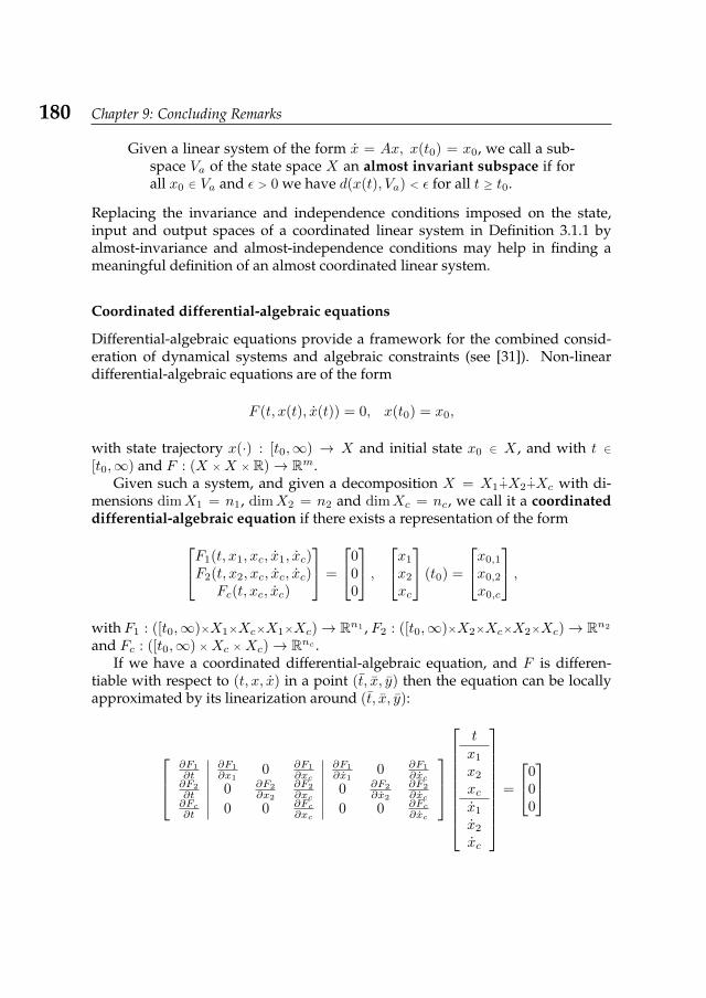
180 Chapter 9: Concluding Remarks
Given a linear system of the form x = Ax, x(t0) = x0, we call a sub-space Va of the state space X an almost invariant subspace if forall x0 ∈ Va and ε > 0 we have d(x(t), Va) < ε for all t ≥ t0.
Replacing the invariance and independence conditions imposed on the state,input and output spaces of a coordinated linear system in Definition 3.1.1 byalmost-invariance and almost-independence conditions may help in finding ameaningful definition of an almost coordinated linear system.
Coordinated differential-algebraic equations
Differential-algebraic equations provide a framework for the combined consid-eration of dynamical systems and algebraic constraints (see [31]). Non-lineardifferential-algebraic equations are of the form
F (t, x(t), x(t)) = 0, x(t0) = x0,
with state trajectory x(·) : [t0,∞) → X and initial state x0 ∈ X , and with t ∈[t0,∞) and F : (X ×X × R)→ Rm.
Given such a system, and given a decomposition X = X1+X2+Xc with di-mensions dimX1 = n1, dimX2 = n2 and dimXc = nc, we call it a coordinateddifferential-algebraic equation if there exists a representation of the formF1(t, x1, xc, x1, xc)
F2(t, x2, xc, xc, xc)Fc(t, xc, xc)
=
000
,x1
x2
xc
(t0) =
x0,1
x0,2
x0,c
,with F1 : ([t0,∞)×X1×Xc×X1×Xc)→ Rn1 , F2 : ([t0,∞)×X2×Xc×X2×Xc)→ Rn2
and Fc : ([t0,∞) ×Xc ×Xc)→ Rnc .If we have a coordinated differential-algebraic equation, and F is differen-
tiable with respect to (t, x, x) in a point (t, x, y) then the equation can be locallyapproximated by its linearization around (t, x, y):
∂F1
∂t∂F1
∂x10 ∂F1
∂xc∂F1
∂x10 ∂F1
∂xc∂F2
∂t 0 ∂F2
∂x2
∂F2
∂xc0 ∂F2
∂x2
∂F2
∂xc∂Fc∂t 0 0 ∂Fc
∂xc0 0 ∂Fc
∂xc
tx1
x2
xcx1
x2
xc
=
000
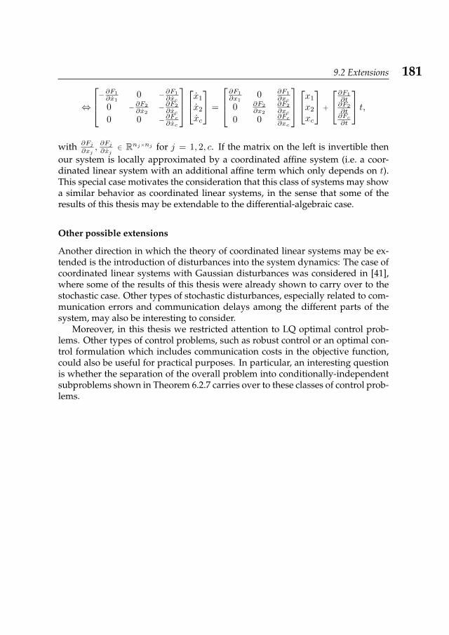
9.2 Extensions 181
⇔
−∂F1
∂x10 −∂F1
∂xc
0 −∂F2
∂x2−∂F2
∂xc
0 0 −∂Fc∂xc
x1
x2
xc
=
∂F1
∂x10 ∂F1
∂xc
0 ∂F2
∂x2
∂F2
∂xc
0 0 ∂Fc∂xc
x1
x2
xc
+
∂F1
∂t∂F2
∂t∂Fc∂t
t,with ∂Fj
∂xj,∂Fj∂xj
∈ Rnj×nj for j = 1, 2, c. If the matrix on the left is invertible thenour system is locally approximated by a coordinated affine system (i.e. a coor-dinated linear system with an additional affine term which only depends on t).This special case motivates the consideration that this class of systems may showa similar behavior as coordinated linear systems, in the sense that some of theresults of this thesis may be extendable to the differential-algebraic case.
Other possible extensions
Another direction in which the theory of coordinated linear systems may be ex-tended is the introduction of disturbances into the system dynamics: The case ofcoordinated linear systems with Gaussian disturbances was considered in [41],where some of the results of this thesis were already shown to carry over to thestochastic case. Other types of stochastic disturbances, especially related to com-munication errors and communication delays among the different parts of thesystem, may also be interesting to consider.
Moreover, in this thesis we restricted attention to LQ optimal control prob-lems. Other types of control problems, such as robust control or an optimal con-trol formulation which includes communication costs in the objective function,could also be useful for practical purposes. In particular, an interesting questionis whether the separation of the overall problem into conditionally-independentsubproblems shown in Theorem 6.2.7 carries over to these classes of control prob-lems.

182 Chapter 9: Concluding Remarks
Bibliography
[1] J. Anderson, A. Teixeira, H. Sandberg, and A. Papachristodoulou. Dynami-cal system decomposition using dissipation inequalities. In Proc. 50th IEEEConference on Decision and Control (CDC.2011), pages 211–216, 2011.
[2] K.J. Arrow and L. Hurwicz. Decentralization and computation in resourceallocation. Essays in Economics and Econometrics, pages 34–104, 1960.
[3] T. Basar. Optimum coordination of linear interconnected systems. Large ScaleSystems, 11(1), 1980.
[4] O. Boutin, J. Komenda, T. Masopust, K. Schmidt, and J.H. van Schuppen.Hierarchical control with partial observations: Sufficient conditions. In Proc.50th IEEE Conference on Decision and Control (CDC.2001), pages 1817–1822,2011.
[5] J.H. Chow (ed.). Time-Scale Modeling of Dynamic Networks with Applications toPower Systems. Springer Verlag, 1982.
[6] J.B. Cruz, Jr. Leader-follower strategies for multilevel systems. IEEE Trans-actions on Automatic Control, AC-23(2), 1978.
[7] R. Cui, S. S. Ge, B. V. E. How, and Y. S. Choo. Leader-follower formation con-trol of underactuated autonomous underwater vehicles. Ocean Engineering,37, 2010.
[8] E.J. Davison and Ü. Özgüner. Characterizations of decentralized fixedmodes for interconnected systems. Automatica, 19(2):169–182, 1983.
[9] J.M. Dion, C. Commault, and J. van der Woude. Generic properties andcontrol of linear structured systems: a survey. Automatica, 39:1125–1144,2003.
[10] W. Findeisen, F.N. Bailey, M. Brdeys, K. Malinowski, P. Tatjewski, and J. Woz-niak. Control and coordination in hierarchical systems. Wiley, Chichester, 1980.
[11] R. Ghabcheloo, A. Aguiar, A. Pascoal, C. Silvestre, I. Kaminer, and J. Hes-panha. Coordinated path-following in the presence of communication lossesand time delays. SIAM Journal on Control and Optimization, 48(1):234–265,2009.
[12] I. Gohberg, P. Lancaster, and L. Rodman. Invariant subspaces of matrices withapplications. John Wiley & Sons, Inc., New York, NY, USA, 1986.
184 Bibliography
[13] W.P.M.H. Heemels, M.C.F. Donkers, and A.R. Teel. Periodic event-triggeredcontrol based on state feedback. In Proc. 50th IEEE Conference on Decision andControl (CDC.2011), pages 2571–2576, 2011.
[14] W.P.M.H. Heemels, J.H. Sandee, and P.P.J. van den Bosch. Analysis ofevent-driven controllers for linear systems. International Journal of Control,81(4):571–590, 2012.
[15] W.P.M.H. Heemels, A.R. Teel, N. van de Wouw, and D. Nešic. Networkedcontrol systems with communication constraints: Tradeoffs between trans-mission intervals, delays and performance. IEEE Transactions on AutomaticControl, 55(8):1781–1796, 2010.
[16] Y.C. Ho. Team decision theory and information structures. In Proc. IEEE,volume 68, pages 644–654, 1980.
[17] Y.C. Ho, P. Luh, and R. Muralidharan. Information structure, Stackelberggames, and incentive controllability. IEEE Transactions on Automatic Control,26(2):454–460, 1981.
[18] J.A. Jacquez. Compartmental Analysis in Biology and Medicine. The Universityof Michigan Press, Ann Arbor, 2nd edition, 1985.
[19] R. Jurdak, P. Baldi, and C.V. Lopes. Adaptive low power listening for wire-less sensor networks. IEEE Transactions on Mobile Computing, 6(8), 2007.
[20] R.E. Kalman. Contributions to the theory of optimal control. Boletin SociedadMatemática Mexicana, 5:102–119, 1960.
[21] R.E. Kalman. Mathematical description of linear dynamical systems. SIAMJournal on Control and Optimization, 1(2):152–192, 1963.
[22] P.L. Kempker, A.C.M. Ran, and J.H. van Schuppen. LQ optimal control forcoordinated linear systems. submitted.
[23] P.L. Kempker, A.C.M. Ran, and J.H. van Schuppen. Construction of a coor-dinator for coordinated linear systems. In Proc. European Control Conference(ECC.2009), pages 4979–4984. Budapest, 2009.
[24] P.L. Kempker, A.C.M. Ran, and J.H. van Schuppen. A formation flying algo-rithm for autonomous underwater vehicles. In Proc. 50th IEEE Conference onDecision and Control (CDC.2011), pages 1293–1298. Orlando, FL, USA, 2011.
[25] P.L. Kempker, A.C.M. Ran, and J.H. van Schuppen. Controllability and ob-servability of coordinated linear systems. Linear Algebra and Its Applications,437:121–167, 2012.
Bibliography 185
[26] P.L. Kempker, A.C.M. Ran, and J.H. van Schuppen. A linear-quadratic co-ordination control procedure with event-based communication. In Proc. 4thIFAC Conference on Analysis and Design of Hybrid Systems (ADHS.2012), pages13–18, 2012.
[27] J. Komenda, T. Masopust, and J.H. van Schuppen. Synthesis of safe sub-languages satisfying global specification using coordination scheme fordiscrete-event systems. In Proc. 10th International Workshop on Discrete EventSystems (WODES.2010), 2010.
[28] J. Komenda, T. Masopust, and J.H. van Schuppen. Supervisory control syn-thesis of discrete-event systems using a coordination scheme. Automatica,48(2):247–254, 2012.
[29] J. Komenda and J.H. van Schuppen. Coordination control of discrete-event systems. In Proc. 9th International Workshop on Discrete Event Systems(WODES.2008), pages 9 –15, 2008.
[30] A. Kotsialos and M. Papageorgiou. A hierarchical ramp metering con-trol scheme for freeway networks. In Proc. American Control Conference(ACC.2005), pages 2257–2262, 2005.
[31] P. Kunkel and V. Mehrmann. Differential-Algebraic Equations. EuropeanMathematical Society, 2006.
[32] G. Lafferriere, A. Williams, J. Caughman, and J. J. P. Veerman. Decentralizedcontrol of vehicle formations. Systems & Control Letters, 54:899–910, 2005.
[33] P. Lancaster and L. Rodman. Algebraic Riccati Equations. Clarendon Press,Oxford, 1995.
[34] D. Lindner, W.R. Perkins, and J. Medanic. Chained aggregation and three-control-component design: a geometric analysis. International Journal of Con-trol, 35(4):621–635, 1982.
[35] Y.Y. Liu, J.J. Slotine, and A.L. Barabási. Controllability of complex networks.Nature, 473:167–173.
[36] J. Lunze and D. Lehmann. A state-feedback approach to event-based control.Automatica, 46(1):211–215, 2010.
[37] S. Martini, M. Egerstedt, and A. Bicchi. Controllability decompositions ofnetworked systems through quotient graphs. In Proc. 47th IEEE Conferenceon Decision and Control (CDC.2008), 2008.
[38] M. Mazo and P. Tabuada. On event-triggered and self-triggered control oversensor/actuator networks. In Proc. 47th IEEE Conference on Decision and Con-trol (CDC.2008), pages 435–440, 2008.
186 Bibliography
[39] M. Moradzadeh, L. Bhojwani, and R. Boel. Coordinated voltage control viadistributed model predictive control. In Proc. Chinese Control and DecisionConference (CCDC.2011), pages 1612 –1618, 2011.
[40] L. Padulo and M.A. Arbib. System theory: A unified state-space approach tocontinuous and discrete systems. Saunders, Philadelphia, 1974.
[41] N. Pambakian. LQG coordination control. Master’s thesis, TU Delft, 2011.
[42] M. Papageorgiou, H. Hadj-Salem, and F. Middelham. ALINEA local rampmetering: Summary of field results. Transportation Research Record: Journal ofthe Transportation Research Board, 1603:90–98, 2007.
[43] G.J. Pappas, G. Lafferriere, and S. Sastry. Hierarchically consistent controlsystems. IEEE Transactions on Automatic Control, 45(6):1144–1160, 2000.
[44] G. Parlangeli and G. Notarstefano. On the reachability and observability ofpath and cycle graphs. In Proc. 49th IEEE Conference on Decision and Control(CDC.2010), 2010.
[45] R. Radner. Team decision problems. Annals of Mathematical Statistics, 33(3),1962.
[46] A. Rahmani, M. Ji, M. Mesbahi, and M. Egerstedt. Controllability of multi-agent systems from a graph theoretic perspective. SIAM Journal on Controland Optimization, 48(1):162–186, 2009.
[47] A.C.M. Ran and L. Rodman. Ranges of Sylvester maps and a minimal rankproblem. Electronic Linear Algebra, 20:126–135, 2010.
[48] A.C.M. Ran and J.H. van Schuppen. Control for coordination of linear sys-tems. In Proc. International Symposium on the Mathematical Theory of Networksand Systems (MTNS.2008; CD-ROM only), 2008.
[49] A. Rantzer. Linear quadratic team theory revisited. In Proc. American ControlConference (ACC.2006), pages 1637–1641, 2006.
[50] M. Rotkowitz and S. Lall. A characterization of convex problems in de-centralized control. IEEE Transactions on Automatic Control, 51(2):1984–1996,2006.
[51] V.R. Saksena, J.B. Cruz, W.R. Perkins, and T. Basar. Information inducedmultimodel solutions in multiple decisionmaker problems. IEEE Transac-tions on Automatic Control, 28(6):716–728, 1983.
[52] N.R. Sandell, Jr., P. Varaiya, M. Athans, and M.G. Safonov. Survey of de-centralized control methods for large-scale systems. IEEE Transactions onAutomatic Control, 23(2):108–128, 1978.
Bibliography 187
[53] C.W. Scherer. Structured finite-dimensional controller design by convex op-timization. Linear Algebra and its Applications, 351–352:639–669, 2002.
[54] P. Shah and P.A. Parrilo. An optimal controller architecture for poset-causalsystems. submitted.
[55] P. Shah and P.A. Parrilo. A partial order approach to decentralized control.In Proc. 47th IEEE Conference on Decision and Control (CDC.2008), 2008.
[56] P. Shah and P.A. Parrilo. H2-Optimal decentralized control over posets: Astate-space solution for state-feedback. In Proc. 49th IEEE Conference on Deci-sion and Control (CDC.2010), pages 6722–6727, 2010.
[57] D.D. Šiljak. Decentralized Control of Complex Systems, volume 184 of Mathe-matics in Science and Engineering. Academic Press, San Diego, 1991.
[58] M.G. Singh. Dynamical Hierarchical Control. North-Holland, Amsterdam (re-vised edition), 1980.
[59] J. Sousa and F. Pereira et al. C4C project - Task WP2.3 Single vehicle operations.C4C Deliverable, FP7-ICT-2007.3.7, www.c4c-project.eu/uploads/files/d-wp2-3.pdf.
[60] C. Stöcker, J. Lunze, and D. Vey. Stability analysis of interconnected event-based control loops. In Proc. 4th IFAC Conference on Analysis and Design ofHybrid Systems (ADHS.2012), pages 58–63, 2012.
[61] J. Swigart and S. Lall. Optimal synthesis and explicit state-space solutionfor a decentralized two-player linear-quadratic regulator. In Proc. 49th IEEEConference on Decision and Control (CDC.2010), pages 132–137, 2010.
[62] H.G. Tanner. On the controllability of nearest neighbor interconnections. InProc. 43rd IEEE Conference on Decision and Control (CDC.2004), pages 2467–2472, 2004.
[63] H.L. Trentelman, A.A. Stoorvogel, and M.L.J. Hautus. Control Theory for Lin-ear Systems. Communications and Control Engineering. Springer, London,2001.
[64] E. Tse, W.R. Perkins, and J. Medanic. Hierarchical control of large scale sys-tems by chained aggregation. In Proc. IFAC Symposium on Large Scale systems:Theory and Applications, pages 203–210, 1980.
[65] H. van de Water and J. Willems. The certainty equivalence property instochastic control theory. IEEE Transactions on Automatic Control, 26:1080–1087, 1981.
188 Bibliography
[66] M. van den Berg. Integrated Control of Mixed Traffic Networks using ModelPredictive Control. PhD thesis, TU Delft, 2010.
[67] J.H. van Schuppen, O. Boutin, P.L. Kempker, J. Komenda, T. Masopust,N. Pambakian, and A.C.M. Ran. Control of distributed systems: Tutorialand overview. European Journal of Control, 17:579–602, 2011.
[68] H. von Stackelberg. Marktform und Gleichgewicht. Springer Vienna, 1934.
[69] J.C. Willems. Almost invariant subspaces: An approach to high gain feed-back design – part 1: Almost controlled invariant subspaces. IEEE Transac-tions on Automatic Control, AC-26:235–252, 1981.
[70] R. Willems. A numerical approach to LQ control for coordinated linear sys-tems. Master’s thesis, Vrije Universiteit Amsterdam, 2012.
[71] H.S. Witsenhausen. A counterexample in stochastic optimum control. SIAMJournal on Control, 6(1):131–147, 1968.
[72] W.M. Wonham. Linear multivariable control: A geometric approach. Springer-Verlag, Berlin, 1979.
[73] Y. Yuan, W. Daamen, S.P. Hoogendoorn, and J.L.M. Vrancken. Coordinationconcepts for ramp metering control in a freeway network. In Proc. 12th IFACSymposium on Transportation Systems, pages 612–618, 2009.
[74] Y. Yuan, W. Daamen, S.P. Hoogendoorn, and J.L.M. Vrancken. Coordinationof agent-based control in a freeway network. In Proc. 21th Chinese Controland Decision Conference (CCDC.09), pages 2284–2290, 2009.
[75] Y. Yuan, J.L.M. Vrancken, W. Daamen, and S.P. Hoogendoorn. Coordinatedramp metering: a case study with the HERO algorithm. In Proc. 16th ITSWorld Congress and Exhibition on Intelligent Transport Systems and Services,pages 1–5, 2009.
Samenvatting (Dutch Summary)
Gecoördineerde regeling van lineaire systemen
Gecoördineerde lineaire systemen zijn decentrale lineaire systemen met een spe-cifieke structuur: Zij bestaan uit drie of meer deelsystemen, waarvan er één de rolvan een coördinator speelt voor de andere deelsystemen. De communicatiestruc-tuur weerspiegelt deze rolverdeling: De coördinator kan de andere deelsystemenbeïnvloeden, maar de andere deelsystemen hebben geen invloed op de coördi-nator of op elkaar. Een gecoördineerd lineair systeem representeert dus één af-takking in een hierarchisch lineair systeem, met een gerichtte boom als commu-nicatiestructuur.
Mogelijke toepassingen van gecoördineerde lineaire systemen omvatten de-centrale systemen met een inherente hierarchische structuur, zoals verkeers-netwerken of elektriciteitsnetwerken, maar ook andere decentrale systemen dieeen hierarchische aanpak toelaten, zoals groepen of formaties van gedeeltelijk-autonome voertuigen. Bovendien kunnen ongestructureerde lineaire systemenvaak in meerdere deelsystemen met een hierarchische structuur worden ontbon-den, om de complexiteit van bijbehorende regelproblemen to reduceren.
Het in dit proefschrift beschreven onderzoek focust op de volgende vragen:
(1) Hoe kunnen ongestructureerde lineaire systemen, of decentrale systemenmet een niet-hierarchische communicatiestructuur, in gecoördineerde lin-eaire systemen worden onbonden of getransformeerd? Is een gegevengecoördineerd lineair systeem ‘zo decentraal mogelijk’, of kan het –binnende hierarchische structuur– nog verder worden ontbonden?
(2) Welk deelsysteem is regelbaar door welke ingangsvariabele – is een lokaleregelaar voldoende, of is er coördinatie nodig om het gewenste regelge-drag te bereiken? Zijn alle voor de implementatie van de gewenste regelaarnodige meetwaardes lokaal waarneembaar, of is communicatie van dezemeetwaardes vereist?
(3) Kunnen wij voor een gegeven gecoördineerd lineair systeem een rege-laar vinden die tot het gewenste regelgedrag leidt maar ook de hier-archische communicatiestructuur respecteert? Hoe presteert deze rege-laar, vergeleken met ongestructureerde regelaars? Kan de prestatie verbe-terd worden door gebeurtenis-gebaseerde terugkoppeling van de gecoördi-neerde deelsystemen naar de coördinator toe te laten?
In de hoofdstukken 1 en 2 wordt het onderwerp van gecöordineerde lineairesystemen gemotiveerd en geïntroduceerd, en relevante concepten en resultatenuit de klassieke systeem- en regeltheorie worden samengevat. De definitie en
190 Samenvatting (Dutch Summary)
sommige basiseigenschappen van gecoördineerde lineaire systemen worden inhoofdstuk 3 beschreven en met gerelateerde decentrale systemen vergeleken.
Vraag (1) is het onderwerp van hoofdstuk 4: Hier worden expliciete proce-dures voor de transformatie van ongestructureerde of niet-hierarchische lineairesystemen naar gecoördineerde lineaire systemen gegeven. Mogelijke definitiesvan minimaliteit van een gecoördineerd lineair systeem worden voorgesteld, omhet concept van een ‘zo decentraal mogelijk’ systeem te formaliseren.
De in vraag (2) bedoelde verdere onderverdeling van de klassieke con-cepten van regelbaarheid en waarneembaarheid ten opzichte van de verschil-lende deelsystemen, ingangsvariabelen en uitgangsvariabelen wordt in hoofd-stuk 5 beschreven. Hierbij onderscheiden wij tussen onafhankelijk en gezamen-lijk regelbare en waarneembare deelruimtes, om ook het niet-bedoelde effekt vande coördinator op de andere deelsystemen te identificeren. Decomposities van detoestandsruimtes van de deelsystemen volgens deze verfijnde concepten geveninzicht in de vraag welke delen lokaal regelbaar of waarneembaar zijn, en waarcoördinatie of communicatie vereist is.
Vanwege de algemeenheid van de formulering, is vraag (3) makkelijkergesteld dan beantwoord: een wiskundige analyse van het regelgedrag is alleenvoor bepaalde regelproblemen mogelijk. Hoofdstukken 6 en 7 behandelen debeperking van vraag (3) tot LQ (lineair-kwadratische) regelproblemen: In hoofd-stuk 6 construëren wij een lineaire terugkoppeling voor een gecoördineerd lin-eair systeem die een kwadratisch kostenkriterium minimaliseert maar ook decommunicatiestructuur respecteert. De uitbreiding van de toelaatbare regelaarsnaar lineaire terugkoppelingen die, naast de binnen het raam van de communi-catiestructuur beschikbare toestandswaardes, ook over stuksgewijs-konstante be-naderingen van de andere toestandswaardes beschikken, is het onderwerp vanhoofdstuk 7. De hierarchische structuur van het systeem heeft ten gevolg datde lokale regelproblemen voor de deelsystemen onafhankelijk van elkaar op telossen zijn; alleen voor het regelprobleem voor de coördinator is de rest van hetsysteem van belang.
Ter illustratie van de in dit proefschrift ontwikkelde theorie zijn in hoofdstuk8 twee toepassingen uitgewerkt: Eén betreft de formatievlucht van drie onbe-mande onderwatervoertuigen – vanwege de hoge kosten en beperking van on-derwatercommunicatie, is het voordelig één voertuig de rol van de coördinatortoe te wijzen, die zijn positie regelmatig aan de andere twee voetuigen stuurt.Het formatieprobleem is een voorbeeld van het in hoofdstuk 6 besproken LQprobleem. Om de robuustheid tegen storingen en communicatieproblemen teverbeteren, is het voor de andere twee deelsystemen mogelijk feedback aan decoördinator te sturen als zij het referentiesignaal niet kunnen volgen.
De andere toepassing betreft de coördinatie van instroombeperkingen aannaburige opritten van een snelweg: Als de gezamenlijke toestroom de capaciteitoverschrijdt, leidt de instroombeperking tot wachtrijen bij de oprit. Bij een uit-
Samenvatting (Dutch Summary) 191
sluitend lokale regeling van de instroom kunnen de wachttijden bij naburigeopritten uiteenlopen – een effect dat door coördinatie te voorkomen is.