Embed Size (px)
Citation preview

Voting and Information Aggregation
Theories and Experiments in the Tradition of Condorcet
Cristina Rata
Advisor: Dr. Salvador Barberà Sández
Universitat Autònoma de Barcelona
Departament d'Economia i d'Història Econòmica
IDEA
May 2002

for my parents

Acknowledgements It is my supervisor Salvador Barberà that I owe my greatest debt. I feel extraordinarily
lucky and grateful to have had his support during nearly four years. I would like to
thank him for making this thesis possible by bringing literature on the Condorcet Jury
Theorem to my attention and by guiding me through my doctoral research. His critical
commentary on my work has played a major role in both the content and presentation of
my results and arguments.
I am grateful to Jordi Brandts, Matt Jackson, Jordi Massó, Nicolas Melissas and Hervé
Moulin for their helpful comments and suggestions regarding the expository aspects and
arguments of my thesis.
I would like to express my gratitude to the IDEA program of the Department
d’Economia i d’Història Econòmica for giving me the opportunity to study and to write
this thesis.
Special thanks to my friends in Barcelona, and especially to Gemma Sala, who helped
me in many ways. Words alone cannot express the thanks I owe to my mother for her
encouragement during these years.
Lastly, I am grateful to the European Commission (the Phare ACE Programme, project
nº P97-9128-S) for providing financial support for this research.

Contents Introduction .................................................................................................................1
1 Optimal Group Decision Rules: Plurality and Its Extensions ................................... 3
2 Strategic Aspects of Information Aggregation by Plurality Rule ............................ 24
3 Information Aggregation by Plurality Rule: An Experiment ...................................52

1
Introduction This thesis consists of three independent papers that offer a justification for the use of
plurality rule as an optimal way to aggregate information for societies composed of
individuals with common interests but diverse information.
The motivation of this thesis follows a line of research in social choice that dates back
to the French mathematician and political philosopher Jean-Antoine-Nicolas de Caritat,
Marquis de Condorcet (1743-1794). In his attempt to provide support for the existence
of a rationally determined order in the human world, Condorcet argued that all events in
human life and behavior could be actually predicted using the calculus of probabilities.
In his Essai sur l’application de l’analyse à la probabilité des decisions rendues à la
pluralité des voix (1785), Condorcet applied this idea to the area of political decision
making. He posited that social justice would be secured if nations would adopt political
constitutions that facilitate accurate group judgments, and argued that the majority rule
would be the most likely constitutional tool to achieve this goal. Condorcet also
analyzed the probabilities of a tribunal's reaching a correct verdict, and used this to
discuss the qualifications of judges and the best form of a jury for a fair trial.
Condorcet's results have been rediscovered by Black (1958), who used them to
formulate what is now known in the social choice literature as the Condorcet Jury
Theorem, and later by Young (1988, 1995). However, Young provided a deeper
analysis by reinterpreting, correcting and extending Condorcet's results. Since then,
there have been many extensions, generalizations and versions of the Condorcet Jury
Theorem. Piketty (1999) wrote a survey that summarizes the most important results of
these works.
Following this line of research, the first paper of this thesis discusses the conditions
under which plurality rule provides the society with the most likely method to reach
accurate group judgments, when more than two choices are possible1. In this paper, as
in Condorcet's work, it is assumed that voters act honestly.
1 Some time after finishing the first paper, I become aware of the work of Paroush and Ben-Yashar (“Optimal Decision Rules for Fixed-Size Committees in Polychotomous Choice Situations”, Social Choice and Welfare, Vol. 18, 4, 2001, 737-746), who studied a similar model with the one proposed here and with whom I coincide on some of the results.

2
However, natural developments in the theory of voting, that brought in the issues of
incentives and strategic interaction in group decision making, were used to challenge
this assumption. Austen-Smith and Banks (1996) were the first to notice that the
combination of private information and common interests in the framework proposed by
Condorcet might create an incentive for voters to act strategically. This observation led
them to ask the question of whether honest voting is compatible with the Nash
equilibrium behavior in the game induced by majority rule. This issue was also taken up
by other authors. The work of Feddersen and Pesendorfer (1997) was especially
relevant for this thesis. One of the conclusions which emerged from this literature was
that optimal information aggregation is sensitive to the voters' behavior. The second
paper of this thesis advances this problematic by studying voters' behavior in the game
induced by plurality rule.
The interest in real-world institutions, for which voting is an important element, raised
for some time the question of whether voters behave as predicted by the theoretical
models. Another question was of how to deal with the complexity of the strategic
environment. The second paper of this thesis calls for answers to these types of
questions. Since the literature on voting experiments seems to provide reasonable
answers to these questions, the third paper of this thesis uses laboratory experiments to
test the implications of the second paper. In doing so, it extends the work of Ladha,
Miller and Oppenheimer (1996) and Guarnaschelli, McKelvey and Palfrey (2000), who
looked for empirical evidence of strategic behavior in Condorcet-type models.

3
Chapter 1
Optimal Group Decision Rules:
Plurality and Its Extensions
Abstract
This paper offers a justification for the use of plurality rule as an optimal way
to aggregate information for societies composed of individuals with common
interests but with private information. The paper follows and extends a line of
research that was introduced by Condorcet (1785), and which is known in the
social choice literature as the Condorcet Jury Theorem. This allows for a full
characterization of plurality rule and extensions of this rule, such as the
generalized weighted plurality rule, as optimal ways to make decisions in
uncertain situations. Further, it offers Condorcet’s result as a special case.

4
1. Introduction
One argument for the use of voting in making decisions in the presence of uncertainty is
that the society is more likely to give correct answers than any individual is. More
precisely, if individuals in the society have a common interest but they have private
information, then voting may provide the society with mechanisms of aggregating
information that lead to optimal decisions.
This idea inspired one of the earliest models of voting that dates back to Condorcet
(1743-1794). In his Essai sur l’application de l’analyse à la probabilité des decisions
rendues à la pluralité des voix (1785), Condorcet argued that if the objective of the
society is to find the “truth” or the “best” choice in a certain situation, but individuals in
the society make sometimes errors in their judgments about what is the “truth” or what
is “best”, then voting by majority is the most likely method to give optimal results.
Condorcet provided the following examples of situations for which his claim would
work:
• A ruling assembly deciding about establishing a new law. The objective of the
assembly is to make decisions that are in the best interest of the society.
However, the members of the assembly may judge differently the consequences
of the new law for the society.
• A trial by jury, where the truth is either the innocence or the guilt of a defendant.
All members of the jury want to discover the truth, but each of them may
interpret differently the evidence during the trial.
To justify his assertion, Condorcet explored the practical use of the calculus of
probabilities. More precise, his argument was as follows. A group of voters has to
choose between two states of affairs, one of which is objectively correct (for example,
innocence in a trial by jury). Voters have a common interest, namely, they all want to
determine the correct state. To make a decision, voters register their opinions that reflect
their judgments about which of the two states is more likely to be correct. Each voter is
more probable to vote for the correct state than for the incorrect one. Further, voters
have the same probability of making the correct choice. Under these conditions,
Condorcet proved that if voters make their choices independently, then the choice with

5
most votes is the one most likely to be correct. In other words, the majority rule is a
statistically optimal method for aggregating voters’ opinions about a fact. Condorcet
also proved a precursor of the statistical fact now known as the law of large numbers,
showing that the decisions made by majority voting tend to become a complete certainty
as the number of voters becomes large. Condorcet’s findings have been rediscovered by
Black (1958), who used them to formulate what is now known in the social choice
literature as the Condorcet Jury Theorem.
Following Condorcet’s analysis, this paper addresses a more difficult question: which
rule is most likely to produce a correct or best result when there are more than two
states or choices? When extending Condorcet's reasoning to the case of more than two
choices, matters become more complicated. This is because when there are more than
two choices one can address two types of questions. One is to determine which is the
most likely rule to give the correct choice; the second one is to find the ranking of
choices that is most likely to be correct, assuming that one exists. When there are only
two choices, the answer to the second question provides an answer to the first one: the
choice that is most likely to be correct is the top-ranked choice in the ranking most
likely to be correct. One may think that this also holds for the case of more than two
choices. However, Young (1988, 1995)1 argued that this does not hold in most cases.
He provided an example where the most likely to be the correct ranking is given by
Condorcet’s pairwise comparisons method, whereas the most likely to be the correct
choice is given by the Borda scoring method.
The aim of this paper is to provide an answer to the first question: which rule is most
likely to select the correct or best choice from a set of choices containing more than two
elements? However, even in this case, matters are not simple. This is because when
there are more than two choices there is a variety of voting rules that may recommend
different choices. Just to give some examples, consider plurality rule, the Condorcet's
rule, the Borda's rule, approval voting, etc. For the case of two choices, these rules will
all predict the same outcome. The problems arise when there are more than two choices,
as different rules may predict different outcomes. Since a natural extension of majority
1 In the above-mentioned papers, Young provided an excellent review and interpretation of the results in Condorcet’s Essai.

6
rule is plurality rule, the concern here is to find out when is it that the use of plurality
rule is optimal to aggregate information.
The framework used in this paper is one in which a decision maker has to find the
optimal decision rule to aggregate the information provided by a group of individuals
with common interests, but, with different opinions about the correct or the best choice
and possibly with different expertise or abilities to identify this cho ice. Some examples2
are as follows:
• The head of an academic department asks its members’ opinions on which of
several possible candidates to employ. All members in the department agree that
the best candidate would be the one that will publish most in the future.
However, they have different opinions about the potential of each candidate.
• The president of a company believes that demand for one of its products is going
to increase. He asks the executive directors of the company to estimate which of
the available policies is best at meeting this new level of demand. Although
they are on the president’s side, the executive directors disagree about the policy
that is most likely to meet this goal.
It is assumed that the decision maker is a Bayesian and so has beliefs on the set of
possible choices. Before he needs to make a decision, the decision maker learns that he
can get more information from a group of experts. It is assumed that each expert
receives a private signal about the true state of the world and that the signals are
independent draws from a state-dependent distribution. The probability with which an
expert receives the correct signal, i.e., the signal corresponding to the true state of the
world, will give his ability or expertise. In other words, these probabilities parameterize
the informativeness of the experts' signals. The probabilities are subjectively provided
by the decision maker and based on his beliefs about the experts’ abilities. The decision
maker requires the experts to vote for one of the available choices and then uses these
votes as additional information to update his prior beliefs. Finally, the choice that is
most likely to be correct will be the one that maximizes his posterior probability. Under
certain conditions, this choice is the one that has more votes, that is the outcome chosen
by plurality rule. This finding allows for a full characterization of plurality rule as an
2 The examples proposed by Condorcet could also be extended to more than two choices. For instance, in the jury context, one could consider a guilty party among several innocent ones.

7
optimal way to aggregate information. Specifically, Proposition 1 says that plurality rule
is the optimal way to aggregate information if and only if the experts’ ability parameter
is higher than an expression that depends on the number of choices and on the prior
beliefs of the decision maker. When the decision maker’s prior belief is well biased in
one direction, the experts’ ability parameter needs to be at least as high as this belief in
order for plurality rule to aggregate information optimally. An interesting feature of the
condition of Proposition 1 is that it does not depend on the number of experts. Thus,
whenever the condition of Proposition 1 holds, plurality rule is optimal even when the
number of experts becomes large. In addition, the Condorcet Jury Theorem is obtained
as a Corollary of the Proposition 1. These results hold for the case where all experts
have the same probabilities to identify the correct choice. When this assumption is
relaxed, the optimal way to aggregate information is given by the generalized weighted
plurality rule. This rule assigns to each choice a score consisting of the sum of two
terms. The first term depends on the decision maker’s beliefs and on the product
between the plurality score of that particular choice. The second term depends on the
experts’ probabilities of identifying the correct choice. The generalized weighted
plurality rule selects the choice with the highest score. Theorem 2 gives a full
characterization of the generalized weighted plurality rule as an optimal way to
aggregate information. It would be interesting to find the conditions under which
plurality rule is optimal in this context. This is left for further research. However, an
example is given suggesting that plurality rule will be optimal if the probabilities of
different experts’ to make the correct choice are similar.
Related literature
There have been many extensions, generalizations and versions of the Condorcet Jury
Theorem. Some examples include Nitzan and Paroush (1982, 1984), Shapley and
Grofman (1984), Young (1986, 1988, 1995). However, while the problem introduced in
this paper is similar in spirit with the one in the literature mentioned above, there is a
difference in the approach as well as in the interpretation of the concepts. Apart from
the assumption of a Bayesian decision maker, that distinguishes the present analysis
from the classical one, three other aspects deserve attention. First, the analysis in this
paper extends the previous results by allowing for more than two choices. Condorcet
himself allowed for more than two choices and argued that the most likely to be the
correct choice would be given by the majority choice in pairwise comparisons.

8
However, the information (data) required to derive the optimal rule in this paper is
different from the one used by Condorcet. In his model, individuals had to compare the
choices paiwisely, whereas here, the experts have to vote only for one choice. In
addition, Young proved that Condorcet was actually mistaken and argued that if the
data used consisted in pairwise votes, then the most likely to be the correct choice
would be given by the Borda rule. Second, the analysis in this paper allows asymmetry
among alternatives. Although Nitzan and Paroush (1982, 1984), and Shapley and
Grofman (1984), had an attempt to model this, their analysis was for two choices only.
Finally, the concept of the optimal decision rule is different. For instance, Nitzan and
Paroush (1982, 1984) defined the optimal decision rule as the rule that maximizes the
expected utility of the group. Young (1985) proposed that the optimal decision rule3
should select that choice that maximizes a likelihood function. In the present paper, the
optimal decision rule is defined as the rule that selects the choice that maximizes the
decision maker’s posterior probability of selecting the correct choice.
Another line of research analyzed whether Condorcet's result continues to hold when
the game induced by the majority rule is played by rational individuals. Research in this
direction includes Austen-Smith and Banks (1996), Feddersen and Pesendorfer (1998),
McLennan (1998), Myerson (1994), Wit (1998) and Coughlan (2000). These works
studied strategic aspects of information aggregation for the 2-choice case,
corresponding to Condorcet's result. A similar approach is used in Rata (2001) to
analyze the strategic aspects of information aggregation for the framework proposed in
the present paper. Finally, Ladha, Miller and Oppenheimer (1996), Guarnaschelli,
McKelvey and Palfrey (2000) and Brandts and Rata (2002) offered experimental results
justifying some of the game theoretical predictions.
The rest of the paper is organized as follows. Section 2 introduces the uncertain multiple
choice model. Section 3 gives the main result of the paper, namely, a characterization
of plurality rule as an optimal way to aggregate information. Section 4 gives the
conditions under which the generalized weighted plurality rule is optimal. The last
section concludes.
3 For the case of equal priors, the concept used here coincides with the one proposed in Young; this is because his approach is similar to Bayesian inference with uniform priors.

9
2. The Uncertain Multiple Choice Model
Choices and States of the World
Consider a finite set of choices A = },...,,{ 21 maaa . Among these choices there is one
that is correct; all the other choices are incorrect. In the examples provided in the
Introduction, this would correspond to: a good candidate or a good policy among bad
ones, a guilty party among innocents, etc. There is a set of possible states of the world
denoted with S = },...,,{ 21 msss , where the state is corresponds to the choice ia being
correct.
Decision Maker
Now there is an individual, the decision maker in what follows, whose purpose is to
identify the correct choice or the true state of the world. In the examples given in the
Introduction the role of the decision maker was played by the head of the academic
department and the president of the company.
Beliefs
Although the decision maker does not know the true state of the world for certain, he is
a Bayesian and, therefore, has beliefs about its identity. These beliefs are given by the
decision maker’s prior probability: )(⋅sp 4. For simplicity, the decision maker’s prior
that the system will be in the state is , )( is sp , is denoted by ip , i.e., )( is sp = ip .
Without loss of generality, it is assumed that 0...1 21 >>>>> mppp .
Experts
Before he needs to make a decision, the decision maker learns that he can get more
information by asking the advice of a group of experts N = },...,2,1{ n . In the examples,
the experts were the members of the department and the executive directors of the
company.
The experts are characterized by their expertise or abilities to identify the correct
choice. A more formal definition of these abilities is provided shortly.
4 According to the subjectivist school of probability, a rational man should organize his beliefs in a way that it is possible to represent those beliefs by probabilities.

10
The decision maker asks each expert in the group N to register his opinion on the
choices in the set A. More precise, each expert has to vote for (abstentions are ruled out)
one choice in the set A.
The vote of an expert t is denoted by tx , where { }mt aaax ,...,, 21∈ .
If the decision maker would not have additional information, he would select the choice
that has the highest prior probability. However, given the additional information
provided by the experts, he can do better. The decision maker performs an informative
experiment to observe the experts' opinions.
Data-generation Process
The data-generation process can be represented in this case by a multinomial
distribution. To see this, consider the following random variable:
iX t = if expert t votes for the choice ia .
For each Nt ∈ , denote by )/Pr( ktt
ik siXq == with { }mki ,...,2,1, ∈ , the probability
with which an expert t votes for the choice ia when the true state of the world is ks . It
should be noted that 1,1
=∑= mi
tikq for any individual i and given the state ks . These
probabilities are interpreted as the expertise or abilities of the experts; they are
subjectively provided by the decision maker and based on his beliefs about the experts'
abilities. The decision maker assumes that the values of the tijq ’s are statistically
independent and that are the same for all experts, that is, ijlij
tij qqq == for any t, l N∈ ,
with lt ≠ . He also assumes that qq ij = whenever ji = and 1
1−
−=
mq
q ij for any i and j
such that ji ≠ . Finally, the decision maker assumes that m
q1
> .
The following holds, ∑=
=mi
ijq,1
1 for any j.
Consider now the random variables 1X , 2X ,..., mX , where:
{ }kXNtX tk =∈= / 5.
5 S denotes the number of elements in the set S.

11
Now if it is to interpret the independent votes of the n experts in the group N as a
sequence of n independent trials of an experiment that has m outcomes, 1a ,..., ka ,..., ma ,
with corresponding probabilities given by 1
1−
−m
q,..., q,...,
11
−−
mq
and frequencies 1X ,...,
kX ,..., mX , then the m-dimensional random variable X = ),...,,( 21 mXXX will be m-
nomial distributed. Furthermore, for a particular sequence of n trials with 1X = 1x , 2X =
2x ,...., mX = mx , the probability function of the m-nomial distribution function will be
given by:
Xp (x / ks ) = k
km
k
xnx
mii
xx
xx
mii m
xn
mq
qm
qm
qx
n−
==
−−
=
−−
−−
−−
∏∏ 11
!!
11
......1
11
1!
!
,1,1
21
,
where ),....,,( 21 mxxxx = .
The probability )/( iX sp ⋅ is interpreted as describing the decision maker’s belief in the
quantity X before the experiment is performed given that he imagines that he knows
which is the true state of the world.
Revision of Beliefs
If he then observes X = x, the decision maker simply updates his prior belief through
Bayes’ theorem:
sp ( ks / x) =
∑∑∏
∏
=
−
−
=
−
∈
−
=
⋅
−−
⋅
−−
=
⋅
−−
⋅
−−
mll
xnx
k
xnx
mll
xnx
mii
k
xnx
mii
pm
pm
pm
xn
pm
xn
ll
kk
ll
kk
,1,1,1
,1
11
11
11
!!
11
!!
.
The posterior distribution )/( xps ⋅ represents the decision maker’s belief about s after
observing X = x.
Optimal Decision Rules
A decision rule is given by d: X → A2 \Ø, where X is the set of voting vectors
),....,,( 21 mxxxx = .
An optimal decision rule is
{ }SsallforxspxspAaxd iikk ∈≥∈= ),/()/(:)(* .

12
In other words, the optimal decision rule selects the choice(s) corresponding to the most
likely to be the true state(s) of the world, i.e., the state(s) maximizing the decision
maker’s posterior probability.
The purpose in what follows is to give a natural interpretation and characterization of
plurality rule as an optimal decision rule.
3. Plurality Rule as an Optimal Decision Rule
The following result provides the optimal decision rule for the model proposed here.
This result is further used to find the conditions under which the optimal decision rule is
plurality rule.
Theorem 1: The optimal decision rule is the weighted plurality rule, that is, the rule
that selects the choice(s) ka with:
−−
+q
qmxp kk 1
)1(lnln ≥
−−
+q
qmxp jj 1
)1(lnln for all kj ≠ .
Proof. See Appendix.
The score assigned to a choice by the weighted plurality rule is given by the sum of a
constant (the logarithm of the decision maker’s priors about each choice being correct)
and the plurality score corresponding to that choice multiplied with some weights (the
logarithm of the decision maker’s priors about individual odds of identifying the correct
choice). Given this, and for certain parameters of the model, the weighted plurality rule
can be interpreted as plurality rule with ties broken in favor of the choice with highest
prior. Specifically, if the decision maker's priors are almost uniformly distributed on the
set of the possible states of the world, then the score associated to a choice by the
weighted plurality rule does not depend on the probability q, as long as m
q1
> , and as a
result the weighted plurality rule will select the choice with highest number of votes.
This is an immediate consequence of the fact that in comparing the scores of two
choices that have almost equal priors the dominant factor will be the plurality score and
not the priors. Moreover, in case of a tie, the weighted plurality rule will select the
choice with highest prior. In other words, if the priors are not too different and m
q1
> ,

13
then the optimal voting rule will be given by plurality rule with ties broken in favor of
the choice with the highest prior. The intuition is simple: if two choices (or more) get
the same number of votes, then the designer of the decision rule should take into
account only his priors. The next result states precisely when plurality rule is optimal.
Proposition 1: Given a vector of priors ),...,,( 21 mppp with mppp >>> ....21 , then
plurality rule with ties broken in favor of the choice with highest prior is the optimal
decision rule for the above problem iff 1
1
)1( ppmp
qm +−
> .
Proof. See Appendix.
Remark 1: The condition of Proposition 1 has a very interesting feature, namely, it
depends only on the extreme priors 1p and mp , not on the other ip 's. This is because
the only relevant situations in deriving this condition are those in which the choice ma
receives the highest number of votes and the choice 1a receives one vote less than the
choice ma . In what follows, such a situation will be called a situation of “almost ties”.
The condition of Proposition 1 insures that in a situation of almost ties, plurality rule
selects the choice ma despite of its possible very low prior. This argument is made more
precise in the proof of Proposition 1.
Remark 2: The condition of Proposition 1 does not depend on the number of experts n
in the voting process. This can be explained by using a similar argument with the one in
Remark 1. The condition does not depend on the number of experts because the only
relevant situations are those in which there are almost ties. However, the total number of
the experts is irrelevant for these situations. This, in turn, implies that Proposition 1
holds as the number of experts become large.
Remark 3: If mpp ≅1 (almost equal priors), then the condition in Proposition 1
becomes m
q1
> , that is, plurality rule will be generally optimal. This is a consequence
of the fact that, when the priors are almost equal, the only relevant information to the
decision maker is the number of votes for a choice. Further, if the prior gets stronger,

14
namely, mp
p1 increases, then the expertise or ability parameter q must also increase for
plurality rule to stay optimal. This says that for plurality rule to be optimal, the quality
of the information q available to the experts should increase with the difference between
the highest prior 1p and the smallest prior mp .
Corollary 1: For 2=m , the majority rule with ties broken in favor of the choice with
higher prior is optimal iff 1pq > .
Proof. See Appendix.
Remark 4: For 2=m and for the case in which the priors are almost equal, 21 pp ≅ ,
the condition in Proposition 1 becomes 21
>q and, thus it gives Condorcet's result as a
particular case.
The following example helps to understand the issues discussed in this section.
Example 1: Consider 3 choices. Assume that the decision maker's priors are given by:
.34, .335 and .325. Then, the optimal decision rule will be given by plurality rule with
ties broken in favor of the choice with highest prior, provided that 34.>q . To see this,
notice that plurality rule is optimal if the following inequalities hold:
34.ln +
xk 12
ln < 335.ln +
−
+q
qxk 1
2ln)1(
34.ln +
xk 12
ln < 325.ln +
−
+q
qxk 1
2ln)1(
335.ln +
xk 12
ln < 325.ln +
−
+q
qxk 1
2ln)1( .
In other words, the optimal decision rule will not select a choice with higher prior if
there is another choice with higher plurality score, or number of votes, available.
The above inequalities are equivalent to:
−<
12
335.34.
, q
q−
<12
325.34.
and q
q−
<12
325.335.
, or 34.>q .

15
Furthermore, if the priors are given by .5, .3 and .2, then plurality rule with ties broken
in favor of the choice with highest prior will be optimal only if 55.>q . At last, for
plurality rule with ties broken in favor of the choice with highest prior to be optimal
when the priors are .6, .25 and .15, the ability parameter has to be 66.>q .
The results of this section provided a formal justification for the use of plurality rule as
an optimal way to make decisions for situations in which individuals have common
interests. For any number of individuals in the group, the probability with which
plurality rule is optimal is not necessarily high. However, whenever it is optimal, it
makes the correct decision with very high probability.
4. Generalized Weighted Plurality Rule as an Optimal Decision Rule
This section relaxes the assumption that experts have equal probabilities of identifying
the correct choice or true state of the world. In what follows, experts in the group N will
be organized into subgroups. More precisely, the experts with equal probabilities of
identifying the true state of the world, tq , will be assigned to the subgroup tN . It is
assumed that ñ such subgroups are possible, with ñ ≤ n. Denote these subgroups with
1N , 2N ,..., ñN and the size of the subgroup lN with ll Nn = . It is assumed that the
values of the tq ’s are statistically independent and that tq > m1
.
Using a similar reasoning with the one in the previous section, it is possible to construct
for each },...,1{ ñl ∈ the m-nomial distributed random variable lX = ),...,,( 21lm
ll XXX ,
where:
{ }kXNtX tl
lk =∈= / .
Then, for a particular sequence of ln trials with lX1 = lx1 , lX2 = lx2 ,..., lmX = l
mx , the
probability function of the m-nomial distribution function will be given by:
lXp ( lx / ks ) =
{ }
( )lkll
k
xnlxl
mi
li
l
mq
qx
n−
∈
−−
∏ 11
!!
,...1
,
where ),....,,( 21lm
lll xxxx = .
Then from the independence assumption, it follows that:

16
Xp (x / ks ) = ( )∏∏=
−
=
−−
ñl
xnlxl
mi
li
l
lkll
k
mq
qx
n
,1,1
11
!!
= ( )∏∏ ∏
∏
=
−
= =
=
−
−
ñl
xnlxl
ñl mi
li
ñll
lkll
k
mq
qx
n
,1,1 ,1
,1
11
!
!.
The posterior probability becomes:
sp ( ks / x) =
( )
( )∑ ∏∏ ∏
∏
∏∏ ∏
∏
= =
−
= =
=
=
−
= =
=
−−
−
−
mjj
ñl
xnlxl
ñl mi
li
ñll
kñl
xnlxl
ñl mi
li
ñll
pm
x
n
pm
x
n
ljll
j
lkll
k
,1 ,1,1 ,1
,1
,1,1 ,1
,1
11
!
!
11
!
!
.
The optimal decision rule for this problem will select the choice(s) ka corresponding to
the most probable state(s) of the world, i.e., the state(s) for which the above expression
is maximal6:
( ) kñl
xnlxl pm
lkll
k∏=
−
−−
,1 11
.
Theorem 2: The decision optimal decision rule is the generalized weighted plurality
rule, that is, the rule that selects the choice(s) ka that satisfies:
kpln +
−−
∑=
l
l
ñl
lk
qqm
x1
)1(ln
,1 ≥ jpln +
−−
∑=
l
l
ñl
lj
qqm
x1
)1(ln
,1 for all kj ≠ .
Proof: See Appendix.
Further, it would be interesting to find the condit ions under which plurality rule is the
optimal decision rule in this more complex framework. However, given the high
number of parameters in this section, this is a difficult task. Nonetheless, the following
example provides some hints in this direction.
Example 2: Consider 8 experts and m choices. The experts are organized in three
groups according to their ability parameter, which is given by one of the following three
probabilities: 1q , 2q and 3q . Without loss of generality, it is assumed that these
6 This expression is proportional to the decision maker’s posterior probability.

17
probabilities can be ordered as follows: 321 qqq ≥≥ . Then, the score associated to a
choice ia by the generalized weighted plurality rule is:
ipln +
−−
1
11
1)1(
lnq
qmx i +
−−
2
22
1)1(
lnq
qmx i +
−−
3
33
1)1(
lnq
qmx i .
For plurality rule to be optimal, the selected choice needs to have the highest number of
votes. As in the previous section, this will require a comparison of the scores of the
"extreme" choices - 1a and ma - in situations of almost ties. In the example considered
here, such a situation would arise for 43 =mx and 311 =x , meaning that there are four
experts with (the lowest) ability 3q voting for the least probable choices ma and three
experts with (the highest) ability 1q voting for the most probable choice 1a . Thus,
plurality rule is optimal iff:
mpln +
−−
3
3
1)1(
ln4q
qm > 1ln p +
−−
1
1
1)1(
ln3q
qm.
After rearranging terms, the above inequality becomes:
−⋅
−⋅
−−<
3
33
1
1
3
31
11
1)1(
mpp
m
,
or, alternatively,
1
3
1
1
3
3
13
11
)1( ppq
qm
pq
m +⋅
−⋅
−−
> .
Since 31 qq ≥ , it follows that 11
1 1
1
3
3
≤−
⋅− q
q. Further, since
mpp11< , for the above
inequality to be satisfied, the expression 1
1
3
3 11 q
q −⋅
− must be very close to 1.
However, this happens only if 31 qq ≅ , namely, the abilities of the individuals are very
similar to each other. In this case, the above inequality will take a similar form to the
one found in Proposition 1. In conclusion, Example 2 suggests that plurality rule will be
optimal if the ability parameters will be very similar to each other and if the smallest
ability parameter is not too small.

18
5. Conclusions and Further Research
The paper has followed and extended a line of research that has been introduced by
Condorcet (1785). Specifically, the framework used in this paper was one in which a
Bayesian decision maker had to find the optimal decision rule to aggregate the
information provided by a group of individuals with common interests, but, with
different opinions about the correct or the best choice and possibly with different
expertise or abilities to identify this choice. This has led to full characterizations of
plurality rule and extensions of this rule, such as, the generalized weighted plurality
rule, as optimal rules to aggregate experts’ opinions.
One assumption in this model has been that the experts vote in an informative and
objective manner. This is equivalent to assuming that an expert’ choice depends only on
his private information, and does not depend upon the choices of the other experts
present in the decision making process. In game theoretical language, experts are taken
to vote non-strategically. The incentive to vote strategically may arise because an
expert’s vote only matters when his vote is pivotal and because the information
available to the other experts is relevant for the expert’s decision. However, as already
mentioned in the Introduction, there is some theoretical and experimental evidence that
strategic voting will occur in the presence of private information and common interests.
Austen-Smith and Banks (1996) were the first to argue that non-strategic voting in the
Condorcet’s Jury Theorem may be inconsistent with Nash equilibrium under general
conditions. A similar result was proved by Feddersen and Pesendorfer (1998) for the
specific case of jury procedures in criminal trials. In response to these results, Myerson
(1994), Wit (1998) and Coughlan (2000) have attempted to find conditions under which
non-strategic voting is compatible with Nash equilibrium behavior. A similar approach
is used in Rata (2001) to identify conditions under which non-strategic voting is
consistent with Nash equilibrium behavior for the problem considered here.
APPENDIX
Theorem 1: The optimal decision rule is the weighted plurality rule, that is, the rule
that selects the choices(s) ka with:
−−
+q
qmxp kk 1
)1(lnln ≥
−−
+q
qmxp jj 1
)1(lnln for all kj ≠ . (1)

19
Proof. Assume that the optimal decision rule selects the choice ka . The purpose is to
show that the choice ka satisfies (1). By definition, the optimal decision rule selects the
choice(s) ka corresponding to the state(s) ks such that:
)/()/( xspxsp ik ≥ for all Ssi ∈ .
Alternatively, the optimal decision rule selects the choice(s) with kx such that:
k
xnx p
mq
qk
k
−
−−
11
≥ j
xnx p
mq
qj
j−
−−
11
for any kj ≠ .
However, since the values of the variables that maximize a function also maximize
monotonic transformations of it, and since the function to be maximized contains
exponential terms, it is more convenient to work with the natural logarithm of this
function. Therefore, taking logarithms in the above inequality and then using the
properties of the logarithms, we get that:
qxk ln +
−−
−1
1ln)(
mq
xn k kpln+ ≥ qx j ln +
−−
−1
1ln)(
mq
xn j jpln+ for any
kj ≠ .
Notice that the term
−−
11
lnm
qn can be deleted since it appears in both sides of the
inequality. Thus, the above inequality becomes:
qxk ln
−−
−1
1ln
mq
xk kpln+ ≥ qx j ln
−−
−1
1ln
mq
x j jpln+ for any kj ≠ .
Rearranging the terms in the inequality and using the properties of the logarithms, it
follows that:
kpln +
−−
qqm
xk 1)1(
ln ≥ jpln +
−−
qqm
x j 1)1(
ln for any kj ≠ ,
which proves the result. QED
Proposition 1: Given a vector of priors ),...,,( 21 mppp with mppp >>> ....21 , then
plurality rule with ties broken in favor of the choice with highest prior is the optimal
decision rule for the above problem iff 1
1
)1( ppmp
qm +−
> .
Proof. To prove the statement of the Proposition 1, it is enough to find the values of q
for which weighted plurality rule coincides with plurality rule with ties broken in favor

20
of the choice with higher prior. The proof is done in two steps. First, the result of
Theorem 1 is used to determine the conditions under which weighted plurality coincides
with plurality rule with ties broken in favor of the choice with higher prior. Second, the
values of q for which these conditions are satisfied will be determined.
First step For weighted plurality rule to coincide with plurality rule with ties broken in
favor of the choice with higher prior, the following conditions must be satisfied:
1) if kj xx = and kj pp > for some j and k, and ij xx > for all i with kji ,≠ , then
−−
+q
qmxp jj 1
)1(lnln >
−−
+q
qmxp kk 1
)1(lnln ;
2) if 1+= kj xx and jk pp > for some j and k, and ij xx > for all i with kji ,≠ , then
−−
+q
qmxp jj 1
)1(lnln >
−−
+q
qmxp kk 1
)1(lnln ;
3) if xxx kj += , with ∈x ∗+Z 7, 1>x , and jk pp > for some j and k, and ij xx > for
all i with ji ≠ , then
−−
+q
qmxp jj 1
)1(lnln >
−−
+q
qmxp kk 1
)1(lnln .
The first condition says that, if two choices, ka and ja , have the same highest number
of votes, then the choice with higher prior is selected. This gives the tie-braking rule. A
similar reasoning applies if there are more than two choices with the same highest
number of votes. The second condition says that the choice with the highest number of
votes is selected, and that a choice ka is not selected only because it has a higher prior.
To make the point clear, the priors are used only to break ties. The third condition is a
generalization of the second one and, as it will be shown, it is satisfied whenever
condition 2 is satisfied. In othe r words, conditions 2 and 3 state that the choice with
highest number of votes must be selected.
Second step It consists in finding the values of q for which the above conditions are
satisfied. It is easy to see that the first condition will be satisfied for any value of q. To
find the values of q for which the second condition is satisfied, consider a situation in
7 ∗
+Z is the set of integers.

21
which there are two choices, say ja and ka , such that 1+= kj xx and jk pp > , and
ij xx > for all i with kji ,≠ , then the second condition can be written as:
−−
++q
qmxp kj 1
)1(ln)1(ln >
−−
+q
qmxp kk 1
)1(lnln .
After rearranging the terms, the above inequality becomes:
j
k
pp
qqm
ln1
)1(ln >
−−
.
Since q
qm−−
1)1(
>1 and 1>j
k
pp
, the inequality is equivalent to kj
k
ppmp
q+−
>)1(
. But,
for plurality rule to be optimal, this condition must be true for any j and k with
jk pp > .
Thus, 1
1
:, )1()1(max
ppmp
ppmp
qmkj
k
ppjk jk +−=
+−>
>.
Finally, the third condition is satisfied whenever the second one does. To see this, it is
enough to notice that:
−−
++q
qmxxp kj 1
)1(ln)(ln >
−−
++q
qmxp kj 1
)1(ln)1(ln for any 1>x and any two
choices satisfying condition 3. This proves the result. QED
Corollary 1: For 2=m , the majority rule with ties broken in favor of the choice with
higher prior is optimal iff 1pq > .
Proof. It follows directly from Proposition 1 and the remark that 112
1 ppp
pq =
+> .
Theorem 2: The decision optimal decision rule is the generalized weighted plurality
rule, that is, the rule that selects the choice(s) ka that satisfies:
kpln +
−−
∑=
l
l
ñl
lk
qqm
x1
)1(ln
,1 ≥ jpln +
−−
∑=
l
l
ñl
lj
qqm
x1
)1(ln
,1 for all kj ≠ .
Proof. Assume that the optimal decision rule selects the choice ka . Then it should be
the case that:

22
( ) kñl
xnlxl pm
lkll
k∏=
−
−−
,1 11
≥ ( ) jñl
xnlxl pm
ljll
j∏=
−
−−
,1 11
for all kj ≠ .
Using the same argument with the one in Theorem 1, one can take logarithms in the
above inequality and then use the proprieties of the logarithms, to get that:
∑= ñl
llk qx
,1)ln( + ∑
=
−
−−
ñl
llkl m
qxn
,1 11
ln)( + )ln( kp ≥ ∑= ñl
llj qx
,1)ln( + ∑
=
−
−−
ñl
lljl m
qxn
,1 11
ln)(
+ )ln( jp for all kj ≠ .
Rearranging the terms in the previous inequality, it follows that:
∑=
−−
ñll
llk
qqm
x,1 1
)1(ln + )ln( kp ≥ ∑
=
−−
ñll
llj
qqm
x,1 1
)1(ln + )ln( jp for all kj ≠ ,
which gives the result. QED
References
Austen-Smith, D. and J. Banks (1996), Information Aggregation, Rationality, and the Condorcet Jury Theorem, American Political Science Review, Vol. 90, No. 1, 34-45; Brandts, J. and C. Rata (2002), Information Aggregation by Plurality Rule: An Experimental Analysis, IDEA, Universitat Autònoma de Barcelona; Coughlan, P. J. (2000), In Defense of Unanimous Jury Verdicts: Mistrials, Communication, and Strategic Voting, American Political Science Review, Vol. 94, No. 2, 375-393; Condorcet, Marquis de (1785), Essai sur l’Application de l’Analyse a la Probabilite des Decisions Rendues a la Probabilite des Voix, Imprimerie royale, Paris; Feddersen, T. and W. Pesendorfer (1998), Convicting the Innocent: The Inferiority of Unanimous Jury Verdicts under Strategic Voting, American Political Science Review, Vol. 92, No 1, 23-35; Grofman, B. and L. Shapley (1984), Optimizing Group Judgmental Accuracy in the Presence of Interdependencies, Public Choice 43, 329-343; Guarnaschelli, S., McKelvey R. and T. Palfrey (2000), An Experimental Study of Jury Decision Rules, American Political Science Review, Vol. 94, No. 2, 407-422; Ladha, K., Miller G. and J. Oppenheimer (1996), Information Aggregation by Majority Rule: Theory and Experiments, University of Maryland; Myerson, R.B. (1994), Extended Poisson Games and the Condorcet Jury Theorem, Discussion Paper 1103, The Center For Mathematical Studies in Economics and Management Science, Evason: Northwestern University;

23
Nitzan, S. and J. Paroush (1982), Optimal Decision Rules in Uncertain Dichotomous Choice Situations, International Economic Review, Vol. 23, No. 2, June, 289-297; Nitzan, S. and J. Paroush (1984), The Significance of Independent Decisions in Uncertain Dichotomous Choice Situations, Theory and Decision 17, 47-60; Rata, C. (2001), Strategic Aspects of Information Aggregation by Plurality Rule, IDEA, Universitat Autònoma de Barcelona; Wit, J. (1998), Rational Choice and the Condorcet Jury Theorem, Games and Economic Behavior 22, 364-376; Young, H. P. (1986), Optimal Ranking and Choice from Pairwise Comparisons, in Information Pooling and Group Decision Making, ed. Bernard Grofman and Guillermo Owen, Greenwich, CT: JAI; Young, H. P. (1988), Condorcet’s Theory of Voting, American Political Science Review, Vol. 82, No. 4, 1231-1244; Young, H. P. (1995), Optimal Voting Rules, Journal of Economic Perspectives, Vol. 9, No. 1, 51-64.

24
Chapter 2
Strategic Aspects of Information
Aggregation by Plurality Rule
Abstract
This paper is concerned with rules that aggregate information among
individuals with common interests but private information. Specifically, it
studies optimal information aggregation and individuals' voting behavior in
this context. A rule aggregates information optimally if it selects the choice
that individuals would unanimously agree upon if all the signals describing
the private information were common knowledge. An individual votes non-
strategically if he reveals his private information during the voting process.
It is shown that when plurality rule is optimal, non-strategic voting
constitutes a Bayesian Nash equilibrium of the voting game induced by this
rule. However, this equilibrium coexists with other interesting equilibria,
where revelation does not occur. It is also shown that individuals may find in
their interest to vote non-strategically even when plurality rule is not
optimal.

25
1. Introduction
This paper analyzes information aggregation and voting behavior in environments in
which individuals have private information about which of several available choices
best meets their common interests. Examples of such environments are as follows:
• The members of an academic department have to decide whom of several
possible candidates to employ. All members in the department agree that the
best candidate would be the one that will publish most in the future.
However, they have different opinions about the potential of each candidate.
• The executive directors of a company believe that demand for one of its
products is going to increase. They have to estimate which of the available
policies is best at meeting this new level of demand. However, the executive
directors disagree about the policy that is most likely to meet this goal.
• The members of a jury have to identify the guilty party among several parties.
All members of the jury want to discover the guilty party, but each of them
may interpret differently the evidence during the trial.
As in the above examples, the paper considers a group of individuals that have
common interests: they all want to select the choice that is correct (best candidate,
best policy and guilty party, in the examples). Individuals do not know which is the
correct choice, but they have common priors on the set of choices. In addition, before
they need to make a decision, individuals see a private signal that provides them
additional information about the correct choice. The final decision is reached by
taking a simultaneous vote. Each individual must vote (abstentions are ruled out) for
a single choice. The outcome of the voting process is given by plurality rule with ties
broken in favor of the choice with higher prior. The use of this tie-breaking rule is
very natural. Given their common interests, if individuals would not have additional
information then they would unanimously agree that the choice with the highest prior
should be selected. A situation of ties is similar in the sense that does not provide
much information either.
In this setting, the paper analyses first the conditions under which plurality rule is the
optimal way to aggregate information. The criterion for the optimality is close to the

26
one of the first-best optimum in Informational Economics. Namely, the optimal
voting rule selects the choice that would have been selected if all the private
information were common knowledge. However, this definition assumes that all
individuals reveal truthfully their private information or signals during the voting
process. In other words, individuals are assumed to vote non-strategically. To see
why this may not be the case, consider an individual that sees a signal supporting a
choice with very small prior. Assume further that the signals do not provide the
individuals with much information, and that he knows that. Under these assumptions,
if this individual thinks that his vote can change the outcome of the voting process,
i.e., his vote is pivotal, then he might consider voting for a choice that has higher
prior. This suggests that individuals may have incentives to vote strategically and
motivates the second question of this paper: Do individuals have incentives to reveal
their information during the voting process? To answer this question, the paper
analyses whether non-strategic voting is a Bayesian Nash equilibrium of the common
voting game induced by plurality rule with ties broken in favor of the choice with
highest prior. This also allows for an analysis of optimal information aggregation and
voting behavior in a simple, but realistic, environment.
The paper offers three types of results. First, it provides a full characterization of
plurality rule as an optimal way to aggregate information. In order for plurality rule
to aggregate information optimally, the quality of the information (which measures
the informativness of the signals) available to the individuals must be high enough.
In particular, it has to be higher than an expression that depends on the number of the
choices and the extreme priors. If the quality of the information is not high enough,
an individual that sees a signal corresponding to a high prior choice may not be
willing to agree on the selection of a choice with smaller prior but supported by more
signals. This is further enhanced if the priors are well biased in one direction.
The second result proves that there is a tension between optimal information
aggregation and non-strategic voting. The non-strategic voting behavior takes the
form of informative voting, in which individuals vote according to the signal
received. In this case, individuals reveal their private information through their votes.
It is shown that if plurality rule aggregates information optimally, then informative
voting is a Bayesian Nash equilibrium of the voting game induced by this rule.

27
However, the opposite is not true. Although this seems like a surprising result, the
reason behind it is simple. For plurality rule to be optimal and informative voting to
be an equilibrium, the quality of the information available to the individuals has to be
high. Otherwise, in the first case, an individual that sees a signal corresponding to a
high prior choice is not willing to agree on a small prior choice even if it is supported
by more signals and, in the latter, an individual that sees a signal corresponding to a
small prior choice would vote for the highest prior choice. However, in the latter
case, the quality of the information does not need to be as high as in the first case
since the individual that created problems for the optimal information aggregation
cannot do better than voting informatively.
The third part illustrates some other interesting equilibria that coexist with the
informative equilibrium. These are semi-pooling equilibria in which individuals that
see signals different from the one corresponding to the highest prior choice prefer to
vote for this particular choice. These equilibria are calculated in an example with
three choices and three individuals. The existence of semi-pooling equilibria
reinforces the idea of a tension between optimal information aggregation and
informative voting. It shows that even when optimal information aggregation
requires informative voting, individuals may prefer to use semi-pooling strategies
instead. However, the informative voting equilibrium outperforms the semi-pooling
equilibria even in the interval in which plurality rule is not optimal. More precisely,
if plurality rule is used to aggregate votes then, among all possible equilibria, the
informative one maximizes the probability of selecting the correct choice. This
softens the above-mentioned tension. Unfortunately, the computational complexity
of the equilibria in games with private information makes it difficult to generalize
these findings.
Related Literature
The questions addressed here follow an old literature on information aggregation in
groups that dates back to Condorcet. In his Essai sur l’application de l’analyse à la
probabilité des decisions rendues à la pluralité des voix (1785), Condorcet argued
that, in a two-alternative election in which individuals are equally competent, have
common interests and vote independently, the majority rule is the mechanism of

28
aggregating information that leads to optimal decisions 1. Young (1988, 1995)
provides an excellent review, interpretation and further analysis of Condorcet’s
work. Other variations and extensions include: Berg (1993), Grofman and Feld
(1988), Ladha (1992)2. The results of these papers are statistical in nature.
Another line of research studies the extent to which Condorect’s result continues to
hold when strategic voting is allowed. Austen-Smith and Banks (1996) were the first
to point out that Condorcet’s result might not hold for rational individuals. They
showed that for the majority rule to aggregate optimally the information, non-
strategic voting has to be an equilibrium in the voting game induced by the majority
rule, and vice versa. The issue of strategic voting was taken also by: Myerson (1994),
Feddersen and Pesendorfer (1998), McLennan (1998), Wit (1998) and Coughlan
(2000).
The approach taken here is related to the approach taken by Austen-Smith and Banks
(1996). There are three points of departure from their paper and, in general, from the
literature presented above. First, the paper extends this literature to the case of more
than two choices. This is a very natural extension since there are many real life
situations that entail a selection from more than two choices. Second, the paper
explains the use of plurality rule as an optimal way to aggregate information. A third
departure consists in the use of a rule for breaking ties. In the case of two choices,
ties can be avoided by assuming an odd number of individuals. When there are more
than two choices, the ties become a real issue. To see this, take an example with five
choices and three individuals. In this paper, the issue of ties is solved in an original,
but natural, way. Ties are broken in favor of the choice with higher prior. The use of
this rule was justified at the beginning of this Introduction.
The motivation of this paper is also close to the one in Feddersen and Pesendorfer
(1997). Their concern was with voting behavior and information aggregation in
environments where individuals are uncertain about a state variable. However, their
1 Condorcet’s findings have been rediscovered by Black (1958), who used them to formulate what is now known in the social choice literature as the Condorcet Jury Theorem. 2 See Piketty (1999) for the most recent survey of extensions of Condorcet’s result.

29
paper is different from the present one in several ways. One of them, but not the only
one, is that individuals have different preferences.
Finally, Ladha, Miller and Oppenheimer (1996) and Guarnaschelli, McKelvey and
Palfrey (2000) offer experimental results justifying the game theoretical predictions
of some of the above-mentioned papers. An experimental study for the results
presented here is done in Brandts and Rata (2002).
The rest of the paper is organized as follows. Section 2 introduces the model. Section
3 provides a characterization of plurality rule as an optimal way to aggregate
information. Section 4 allows for strategic behavior and analyses the tension between
information aggregation and informative voting. It also illustrates other voting
equilibria. The last section provides some final remarks.
2. The Model
Consider a set of choices A = },...,,{ 21 maaa . Among these choices there is one that is
correct; all the others are incorrect. In the examples provided in the Introduction, this
would correspond to: a good candidate or a good policy among bad ones, a guilty
party among innocents, etc. There is a set of possible states of the world S =
},...,,{ 21 maaa , where the state ia corresponds to the choice ia being correct.
A group of individuals N = { ,2,... }1 n has to decide on the choice to be selected from
the set A. Individuals have common interests. They all want to identify the correct
choice or the true state of the world.
The true state of the world is unknown, but individuals have common priors over the
set of possible states of the world, given by 1p , 2p ,..., mp , where ip is the prior
probability that ia is the true state of the world. The priors satisfy ∑=
m
jjp
1
= 1. With no
loss of generality, it is assumed that 0....1 21 >>>>> mppp .
Before any decision is made, an individual i receives a private signal { }msi ,...,2,1∈
about the true state of the world. A profile of signals is denoted with

30
),...,,( 21 nssss = . The signal that an individual i receives is correlated with the true
state of the world:
ikjji qaks == )/Pr( ,
where ikjq denotes the probability that the individual i receives the signal k when ja
is the true state of the world. Conditional on the state of the world, the signals
received by different individuals are statistically independent.
It is assumed that qq ikk = and
11
−−
=m
qq i
kj , for any kj ≠ and all Ni ∈ . Thus, the
parameter q gives the probability that individuals receive the "correct" signal and
11
−−q
m is the probability individuals receive any of the remaining m-1 "incorrect"
signals. It is further assumed that )1,/1( mq ∈ , meaning that each individual is more
likely to receive the correct signal than any of the incorrect ones. The last two
observations suggest that the probability q measures the quality of information
received by the individuals, higher q implying higher informativness of the signals.
The final decision is reached by taking a simultaneous vote. Each individual must
vote (abstentions are ruled out) for a single choice in the set A. The choice that
receives the most number of votes is selected and, in case of a tie, the ties are broken
in favor of the choice with higher prior probability. In other words, plurality rule
with ties broken in favor of the choice with higher prior is used to aggregate
individuals’ votes. It should be noted that if individuals would not have additional
information (the signals), then they would unanimous ly vote for the choice with the
highest prior. However, those situations in which two or more choices receive the
same number of votes are similar with those of no private information in the sense
that do not provide much information about the correct choice. This suggests that
breaking ties in favor of the choice with higher prior has a natural interpretation in
this particular environment.
There are m possible plurality outcomes and, as said before, each individual prefers
the outcome that matches the true state of the world. In other words, individuals all
prefer choice ka in state ka . Specifically, if ),( jki aau represents individual i's
utility given the plurality outcome ka and state ja , then:

31
),( kki aau = 1
),( jki aau = 0, for all Ni ∈ .
Since the individuals all have the same utility, the subscripts are dropped from this
function.
All the aspects of the environment described above other than the signals and the
votes are common knowledge.
The purpose in what follows is twofold. The first is to determine the conditions under
which plurality rule with ties broken in favor of the choice with higher prior is the
optimal way to aggregate information. The second is to investigate whether
individuals have incentives to reveal their information during the voting process.
This, in turn, requires an analysis of the strategic aspects of individuals’ behavior in
the common value voting game induced by plurality rule with ties broken in favor of
the choice with higher prior.
3. Plurality Rule as an Optimal Voting Rule
The concern here is with identifying the conditions under which plurality rule is the
optimal way to aggregate information. The starting point is to notice that, in this
particular environment, if individuals would have complete information about the
true state of the world, then they would unanimously agree on the choice to be
selected. Namely, they would select the choice that matches the true state of the
world. Following this idea, a natural way to define an optimal voting rule arises.
The optimal voting rule is defined as the rule selecting the choice that every
individual would select if he were told the signals received by the other individuals3.
In other words, the optimal voting rule selects the choice ka that maximizes the
individuals expected utility when all the signals are perfectly observed:
]),...,,(/),(maxarg 21 njAa
k sssaaEua∈
∈ ,
where [ ] == ∑∈Sa
njjknjkj
sssaaausssaauE )),...,,/(Pr()/(),...,,/(),( 2121
3 This definition of an optimal voting rule, introduced in Austen-Smith and Banks (1996), is close to the concept of first-best optimum in the Informational Economics literature. There, as here, the first-best optimum is one that maximizes an expected utility when all the information is perfectly observed.

32
= =)),...,,/((Pr 21 nk sssaob),...,,(Pr
)(Pr)/),...,,((Pr
21
21
n
kkn
sssobaobasssob
=
=
∑=
m
kkkn
kkn
passsob
passsob
121
21
)/),...,,((Pr
)/),...,,((Pr=
∑=
−
−
−−
−−
m
kk
nnn
k
nnn
pm
pm
kk
kk
1 11
11
, ksNin ik =∈= : .
The last equality follows from the independence of the individuals' signals given the
true state of the world.
The following result gives the condition under which plurality rule is optimal.
Proposition 1: Plurality rule with ties broken in favor of the choice with higher prior
is optimal iff 1
1
)1( ppmp
qm +−
> .
Proof: See Appendix 1.
Proposition 1 says that plurality rule is the optimal way to aggregate information if
and only if the quality of information q available to the individuals is higher than an
expression that depends on the number of choices and the extreme priors. In
particular, when the prior beliefs are well biased in one direction ( 1p is very high),
the quality of the information needs to increase accordingly in order for plurality rule
to aggregate information optimally. This means that, if 1p is high, then it makes
sense to add up votes that go in the same direction only if they bring additional
information, i.e., they are backed by a high q. When the priors are almost uniformly
distributed ( mpp ≅1 ), the only valuable information is provided by the individuals’
votes and, since m
q1
> , the more votes the better. In this case, plurality rule is
optimal most of the time.
The condition of Proposition 1 has some interesting features. First, it does not depend
on the number of the individuals, n. This is because the only relevant situations for
optimal information aggregation are those in which one has to decide whether signals
or priors are more important. Such situations are those of “a lmost ties”, when the

33
choice ma , with the smallest prior, is supported by the highest number of signals and
the choice 1a , with the highest prior, is supported by one signal less than the choice
ma . In a situation of almost ties, the total number of individuals is irrelevant. The
condition of Proposition 1 insures that in a situation of almost ties, plurality rule
selects the choice ma despite of its possible very low prior. This argument is made
more precise in the proof of Proposition 1.
The second interesting feature of the condition in Proposition 1 is that it depends
only on the extreme priors 1p and mp , not on the other ip 's. To provide some
intuition for this result, consider an example with three choices and eight individuals.
In this case, the condition in Proposition 1 becomes 13
1
2 ppp
q+
> . Assume the
following distribution of signals: two ind ividuals see signal 1, another two see signal
2, and four individuals see signal 3. This information is available to everyone. Now,
for an individual receiving signal 1 to agree on the selection of the choice 3a (the
choice supported by most signals), it should be the case that q, the quality of the
signal, is high in general and, in particular, is higher than the prior 1p . Otherwise,
since he has observed a signal corresponding to a choice that has the highest prior, he
would be inclined to believe his signal more than the signals received by the others.
In other words, when a choice with small prior is supported by many signals, an
individual has to be given reasons to put more weight on these signals rather than on
his own signal and the priors. Further, if an individual receiving a signal 1 is willing
to agree on the selection of the choice 3a , supported by more signals but with the
smallest prior, then he will be willing to agree on the selection of 2a , if this choice
would be supported by more signals. This is the reason why the condition in
Proposition 1 depends only on the extreme priors and not on the intermediate ones.
An important consequence of the Proposition 1 is that if individuals reveal their
private information (signals) truthfully, then plurality rule maximizes the likelihood
of making correct decisions whenever the quality of this information is high.
However, it should be noticed that in this case individuals act as if they would
observe perfectly all the signals. This leads to the following question: Would an

34
individual act the same way (reveal his signal) if he assumes that all the others will
reveal honestly their signals, but knowing that he cannot observe these signals? To
see that the answer to this question is not that simple, consider a situation in which
1p (the highest prior) is very high (thus mp is very small) and that the quality of the
information q is a bit higher than 1p . Imagine that an individual sees the signal m
corresponding to the choice with the smallest prior mp . Would he still reveal his
signal by voting for the choice ma ? If he believes his vote to be pivotal, i.e., can
change the outcome of the voting process, then he may very well vote for the choice
1a . Yet, this is not clear and thus motivates the analysis of the strategic aspects of
individuals’ behavior in an environment where plurality rule aggregates optimally
the information. This is the purpose of the following section.
4. Voting Behavior
This section analyses individuals’ voting behavior by looking at the Bayesian Nash
equilibria of the common voting game induced by plurality rule with ties broken in
favor of the choice with higher prior.
The voting game can be described as follows. An individual i observes his type,
which is given by the signal received and is denoted with { }mti ,...,2,1∈ . The type is
privately observed by each individual. Then, the individuals in the group N
simultaneously vote for a choice from the set A. The outcome is given by plurality
rule with ties broken in favor of the choice with higher prior probability. Individuals’
beliefs over the types and expected utilities over the decisions and types are
described in Appendix 2.
The behavior of an individual i is given by a strategy mapping Amv i →},...,2,1{: ,
so that the choice to be selected by an individual i depends on the signal seen or type
it . A voting profile is a mapping nn Amv →},...2,1{: , with ( ) =tv
)).(),...,(),(( 2211 nn tvtvtv
Two types of strategies are of interest here: strategic voting and non-strategic voting.
The non-strategic voting strategy takes the form of informative voting. A voting

35
strategy is informative if ji ajv =)( for any { }mj ,...,2,1∈ . Thus, informative voting
is defined as voting according to the signal received. It should be noted that
informative voting implicitly assumes that the individuals behave as their vote alone
determines the outcome. In addition, when all the individuals adopt informative
strategies all of their private information is revealed during the voting process.
Some remarks are in order now. First, the concern here is with symmetric Bayesian
Nash equilibria, where individuals’ strategies are identical. Thus, the subscripts from
the equilibrium strategies are dropped. Second, as shown in Austin-Smith and Banks
(1990), the equilibrium condition will be trivially satisfied if others use strategies
)(*itv − that never make i pivotal, that is, his vote can change the outcome of the
voting process. Therefore, in computing the decision that is the best response to other
individuals' strategies, an individual should be concerned only with those situations
(type profiles) where his vote is pivotal. Third, the interest here is with equilibria in
pure strategies.
Informative Voting Equilibrium
As previously said, an important issue here is of whether individuals have incentives
to reveal their private information during the voting process. In other words, is
informative voting a Bayesian Nash equilibrium of the voting game introduced
before? The following result gives a sufficient condition for the informative voting to
be a Bayesian Nash equilibrium.
Proposition 2: Plurality rule with ties broken in favor of the choice with higher prior
is optimal implies that informative voting is a Bayesian Nash equilibrium in the
voting game induced by this rule.
Proof: See Appendix 2.
Apart from showing the existence of the informative equilibrium, Proposition 2
points to a surprising aspect of this particular environment, namely, that there is a
tension between optimal information aggregation and informative behavior.
To see that the opposite of Proposition 2 does not hold and to understand what
actually drives the above-mentioned tension, consider the following example.

36
Example 1: Assume three choices and eight individuals (m = 3 and n = 8 in the
model) and the priors 6.1 =p , 25.2 =p and 15.3 =p . By Proposition 1, plurality
rule is optimal iff 66.>q . However, informative voting is an equilibrium for all
54.>q . Thus, for any 66.54. ≤< q , informative voting is an equilibrium but
plurality rule is not optimal. This is actually true for any values of the priors. For
example, when 38.1 =p , 33.2 =p and 29.3 =p (almost equal priors), plurality rule
is optimal for any 39.>q , whereas informative voting is an equilibrium for any
37.>q . This suggests that for equal priors, Proposition 2 may hold in the other
direction too: plurality rule is optimal becoming equivalent with informative voting
being a Bayesian Nash equilibrium in the voting game induced by this rule. The
conditions on q for arbitrary values of 1p , 2p and 3p are provided in Appendix 2.
The example points to an interesting aspect of individuals’ behavior in the game
introduced here. Namely, given that all the other types vote informatively, a type 1
individual will prefer to vote informatively for any q, 1p , 2p and 3p . The reason
for this is simple: if all individuals receiving signals 2 and 3 vote informatively, then
an individual receiving a signal 1 cannot do better than voting informatively since his
signal is also supported by a high prior. However, for a type 2 individual matters are
different. Assuming that the others vote informatively, he faces the trade-off
between: voting for the choice 1a , which is supported by a higher prior, or voting for
the choice 2a , which is supported by his signal. These considerations exclude a vote
for the choice 3a . Similarly, a type 3 individual will face the trade-off between
voting for 1a or 3a . This reasoning turns out to be more general and leads, as it will
be seen next, to interesting results.
Also, the example suggests that the values of q for which plurality rule is optimal and
for which informative voting is an equilibrium are not that different. In both cases q
needs to be high enough. If q is not high enough then, in the first case, individuals
that see a high prior choice cannot agree on a small prior choice even if it is
supported by a majority of signals and, in the second case, individuals that see a
small prior choice would be tempted to vote for the highest prior choice. This is what

37
brings together, though for different reasoning, the optimal aggregation of
information and the informative voting.
Illustrating some Strategic Voting Equilibria
It should be noticed that there might exist other Bayesian Nash equilibria for the
voting game proposed here. For example, the strategy profile where all individuals
are voting for the same choice constitutes a Bayesian Nash equilibrium. To see this,
assume that all individuals other than individual i vote for the choice ka , say. Then
individual i’s vote is irrelevant, since the choice ka will be selected by plurality rule.
There are m such pooling equilibria. However, since at these equilibria an individual
is never pivotal, they all involve weakly dominated strategies and, as argued in
Feddersen and Pesendorfer (1995), elimination of weakly dominated strategies is a
natural refinement. Therefore, applying this argument eliminates all the pooling
equilibria. Nevertheless, there exist other equilibria (in pure strategies) that do not
involve weakly dominated strategies and that turn out to be very interesting and to
have nice interpretation. The following example illustrates such equilibria.
Example 2: Consider three choices and three individuals (m = 3 and n = 3). Fix some
priors 321 ppp >> . In this case, informative voting is an equilibrium iff q satisfies:
2
2
22
12
1
q
qqq
−
+
−
≤1
2
pp
, 2
2
22
12
1
q
qqq
−
+
−
≤1
3
pp
and q
q
−
21
≤2
3
pp
.
The first remark is that informative voting is not the unique equilibrium. There exist
two other equilibria. These are semi-pooling equilibria, in which an individual that
has a low type (or, sees a small prior choice) votes for the choice with the highest
prior. The first semi-pooling equilibrium is one where type 1 and type 2 individuals
vote for the choice 1a and type 3 individuals vote for the choice 3a :
1** )2()1( atvtv ==== , 3
* )3( atv == . Semi-pooling (1)
These strategies constitute an equilibrium for all q such that:
2
2
22
12
1
q
qqq
−+
−
≤1
3
pp
≤q
22
1
−+
.
The other semi-pooling equilibrium is given by the voting strategies:

38
1** )3()1( atvtv ==== , 2
* )2( atv == , Semi-pooling (2)
meaning that types 1 and 3 vote for the choice 1a , whereas type 2 votes for 2a . This
is an equilibrium for all q such that:
2
2
22
12
1
q
qqq
−+
−
≤1
2
pp
≤q
22
1
−+
.
Since the above inequalities are hard to interpret, assume the priors are given by
6.1 =p , 25.2 =p and 15.3 =p . In this case:
Informative voting is an equilibrium for all 57.≥q
Semi-pooling (1) is an equilibrium for all 57.≥q
Semi-pooling (2) is an equilibrium for all 48.≥q .
To see that this is not only a casual happening, consider the priors 5.1 =p , 3.2 =p
and 2.3 =p . Then:
Informative voting is an equilibrium for all 48.≥q
Semi-pooling (1) is an equilibrium for all 48.≥q
Semi-pooling (2) is an equilibrium for all 71.41. ≤≤ q .
The second remark is that these equilibria coexist in the domain of q for which
plurality rule is optimal. When 6.1 =p , 25.2 =p and 15.3 =p :
plurality rule is optimal for all 66.6.15.2
6.=
+∗>q .
When 5.1 =p , 3.2 =p and 2.3 =p :
plurality rule is optimal for all 55.5.2.2
5.=
+∗>q .
Further, it is an easy exercise to show that even in the interval 66.57. << q (where
plurality rule is not optimal), the informative voting equilibrium performs better than
the other two equilibria, in the sense that the probability of making correct decisions
at the informative voting equilibrium is higher than at the other two equilibria. This
alleviates the tension between optimal aggregation information and voting behavior
in common interest environments.
The equilibria for the game introduced here have been calculated also for: m = 3 and
n = 5 and, m = 4 and n = 3. Similar patterns of results with the ones for m = 3 and n

39
= 3 have been observed. Specifically, in each case, there exist semi-pooling
equilibria of the type described above. These equilibria typically coexist with the
informative voting in the domain of q for which plurality rule is optimal.
Interestingly, for the case of four choices (m =4), the semi-pooling equilibria all had
the same structure: types 1 and 2 and/or 3 and/or 4 vote for the choice 1a and all the
others vote informatively. In other words, individuals consider only deviations for
the highest prior choice 1a . This makes sense in this common interests setting: the
deviation has to be in the most plausible direction. Also, these semi-pooling
equilibria and the informative one were the only4 equilibria in pure strategies in these
examples.
5. Final Remarks
This paper has explored the implications of private information for environments in
which individuals have common interests. Specifically, its purpose has been to
identify those aspects of the informational and decisional making environment that
influence whether individuals reveal their information during the voting process. It
has been shown that there is a tension between optimal information aggregation and
informative voting. This is a combination of two factors. One is that, individuals may
find in their interest to vote informatively even when information is not aggregated
optimally. In this direction, it has been shown that plurality rule is optimal implies
that individuals vote informatively, but the opposite does not hold in general. The
other is that, even when optimal information aggregation requires informative voting,
individuals may prefer to use semi-pooling strategies instead. This is supported by
the fact that informative voting equilibrium coexists with semi-pooling equilibria in
the range of q’s for which plurality aggregates information optimally.
Since games with private information are complex, the existence of semi-pooling
equilibria is shown by means of examples. Although these examples are only a
beginning for a more general theoretical analysis, they are enough to support the
above predictions. In that case, the multiplicity of equilibria in this environment calls
for an analysis of the equilibrium selection. One way to examine this would be to
study the stability of the equilibria with respect to some stability notion, such as
4 Of course, apart from the pooling equilibria that were discarded from the beginning.

40
information-proofness (Kalai, 2000). Another way would be to use laboratory
experiments. The latter approach has been taken in Brandts and Rata (2002), where
voting behavior and optimal information aggregation is analyzed for a three-choice
and three- individual environment.
There are other interesting issues that were not considered in this paper. One of them
is the analysis of voting behavior and information aggregation in the domain of q for
which plurality rule is not optimal. Another one is the study of optimal information
aggregation for those situations where individuals vote strategically. These
extensions are left for further research.
Appendix 1
Proposition 1: Plurality rule with ties broken in favor of the choice with higher prior
is optimal iff 1
1
)1( ppmp
qm +−
> .
Proof: The proof is done in two steps.
Step 1: It is shown that the optimal voting rule selects the choice(s) ka for which:
−−
+q
qmnp kk 1
)1(lnln ≥
−−
+q
qmnp jj 1
)1(lnln for all kj ≠ .
Step 2: It is shown that, for plurality rule with ties broken in favor of the choice with
higher prior to be optimal, the conditions derived in Step 1 must reduce to:
1
1
)1( ppmp
qm +−
> .
Step 1: As stated before, the optimal voting rule selects the choice(s) that maximizes
the expected utility of the individuals given the vector of signals ),...,,( 21 nssss = . In
other words, the optimal voting rule selects the choice(s) ka for which the expression
below is maximal:
∑=
−
−
−−
−−
m
ii
nnn
k
nnn
pm
pm
ii
kk
1 11
11
.
or:

41
k
knnkn p
mq
q−
−−
11
≥ i
nnn p
mq
qi
i
−
−−
11
for any ki ≠ .
After taking logarithms in the above inequality and rearranging its terms, the
inequality becomes:
kpln +
−−
qqm
nk 1)1(
ln ≥ ipln +
−−
qqm
n i 1)1(
ln for any ki ≠ .
Thus, the optimal voting rule will select the choice(s) ka whose score:
kpln +
−−
qqm
nk 1)1(
ln is maximal.
Step 2: Plurality rule with ties broken in favor of the choice with higher prior is
optimal if the score attached by this rule to a choice ja is such that:
1)
−−
+q
qmnp jj 1
)1(lnln >
−−
+q
qmnp kk 1
)1(lnln for any ja and ka such that
kj pp > and ikj nnn >= for all i with kji ,≠ ;
2)
−−
+q
qmnp jj 1
)1(lnln >
−−
+q
qmnp kk 1
)1(lnln for any ja and ka such that
ikj nxnn >+= for all i with ji ≠ and ∗+∈ Zx 5, and jk pp > (this condition is
obviously satisfied when kj pp > ).
The first condition gives the tie-breaking rule, that is, if two or more choices have the
same number of votes, then the choice with higher prior should be selected. The
second condition states that the choice with the highest number of votes will always
be selected. Hence, a choice ka will not be selected only because it has a higher
prior.
Further, since 11
)1(>
−−
qqm
, condition 2) needs to be satisfied only for 1=x . It is
easy to see that if condition 2) is satisfied for 1=x , then it will be satisfied for any
1>x . In that case, given two choices ja and ka with 1+= kj nn , jk pp > and
ij nn > for all i, ji ≠ , condition 2) becomes:
5 ∗
+Z is the set of strictly positive integers.

42
−−
++q
qmnp kj 1
)1(ln)1(ln >
−−
+q
qmnp kk 1
)1(lnln .
Furthermore, since q
qm−−
1)1(
>1 and 1>j
k
pp
, the above inequality can be rewritten as
kj
k
ppmp
q+−
>)1(
. But, for plurality rule to be optimal, this condition must be true
for any two choices ja and ka that satisfy condition 2), or alternatively, for any j
and k with jk pp > .
Thus, 1
1
:, )1()1( ppmp
ppmp
maxqmkj
k
jpkpjk +−=
+−>
>. The last equality follows from
the assumption that mppp >>> ....21 . This proves the result. QED
APPENDIX 2
The voting game is described by:
- The set of type profiles (or vectors) iiTT ×= , with each set },...2,1{ mTi = describing
the types of individual i; a type profile will be denoted with ),...,( 1 nttt = or
),( ii ttt −= .
- Individuals’ common preference over the voting profile ))(),...,(()( 11 nn tvtvtv = and
the type profile t :
:))),(),...,((( 11 ttvtvU nn = [ ]tatvtvPLuE nn /))),(),...,(((( 11 =
= )/(Pr))),((( taobatvPLuSa
∑∈
= )/))(),...,((((Pr 11 ttvtvPLaob nn= ,
where ))(),...,((( 11 nn tvtvPL is plurality outcome at ))(),...,(( 11 nn tvtv .
- i's belief describing i's uncertainty about the n-1 other players' possible types, it− ,
given i's own type, it : )/( ii ttp − . This can be done using Bayes rule:
∑∈
−
−− ==
Niiii
iiii ttp
tptp
ttpttp
),()(
)(),(
)/( ,
where
∑ ∏∑= ∈=
==mj Ni
jijmj
jj atobpatobptp,1,1
)/(Pr)/(Pr)(
is the common prior probability of a type profile Tt ∈ .

43
The last equality follows from the independence of the individuals' signals given the
true state of the world.
The expected utility from voting for )( ii tv , given the updated belief )/( ii ttp − and
the strategies of the other players )( ii tv −− is given by:
))(,);(( iiiii tvttvEU −− [ ]∑∑ −−
−=
ii
tt
iittvPLob
ttp&))((Pr
),(1
.
All this is taken to be common knowledge between the individuals. A Bayesian Nash equilibrium (in pure strategies) of the above game is a strategy
profile )(* ⋅v such that for all Ni ∈ and all ii Tt ∈ , ki atv =)(* only if
),;(),;( ** vtaEUvtaEU ijik ≥ for any kj ≠ .
Proposition 2: Plurality rule with ties broken in favor of the choice with higher prior
is optimal implies that informative voting is a Bayesian Nash equilibrium in the
voting game induced by this rule.
Proof: Recall that at a Bayesian equilibrium, every individual makes a decision that
is optimal relative to the distribution of the individuals' types and their decision-
selection rules. Then, at the informative voting equilibrium, an individual makes the
decision that is best relative to the individuals' types and given that all the other
individuals vote informatively.
The conditions for an individual i of type k to vote informatively given that all the
other individuals vote informatively are given by:
[ ] [ ]))(,,())(,;( infinfiiijiiik tvktaUEtvktaUE −−−− =≥= for all kj ≠ ,
where )(infii tv −− is the vector of decisions of all individuals except i according to the
informative strategy profile )(inf ⋅v .
Further, using the remark of Section 4 that at the equilibrium the only relevant type
profiles for individual i are those where he is pivotal, the above conditions can be
rewritten as:
[ ]∑−− ∈
−−−)(
inf ),(&))(,(Prii TPivt
iiik tktvaPLob [ ]∑−− ∈
−−−≥)(
inf ),(&))(,(Prii TPivt
iiij tktvaPLob
(1)

44
for any kj ≠ , where )( iTPiv − is the set of profiles at which an individual i is pivotal
and ),( itk − is the type profile with kti = and )( ii TPivt −− ∈ .
The objective is to show that if plurality rule 6 is optimal, then (1) holds for all
},...,2,1{ mkti ∈= .
To prove this, consider an individual i with kti = , and fix an arbitrary profile
)( ii TPivt −− ∈ .
First, it is proved that if plurality rule is optimal, then the following should hold:
[ ]),(&))(,(Pr infiiik tktvaPLob −−− [ ]),(&))(,(Pr inf
iiij tktvaPLob −−−≥ (2)
for all kj ≠ .
Since the profile it − was arbitrary chosen, if (2) holds at the type profile ),( itk − ,
then it must hold for all type profiles ),( itk − with )( ii TPivt −− ∈ . For the same
reason, (2) should hold for all },...,2,1{ mk ∈ . Further, one can take the sum over all
)( ii TPivt −− ∈ in (2) to obtain (1) for all },...,2,1{ mk ∈ .
To prove (2), consider three choices 1a , 2a and 3a . As it will become clear at the
end of the exposition, a similar reasoning applies for more than three choices.
Denote with ktNin ik =∈= : the number of individuals of type k at a type profile
t. Thus nnmk
k =∑∈ },...,1{
. The same notation was used in Proposition 1 to denote the
number of individuals receiving a specific signal. There is no loss of generality in
using this notation here too, since the types coincide with the signals.
The purpose now is to show that (2) holds for all }3,2,1{∈it and all )( ii TPivt −− ∈ .
Consider each possibility for it :
I) 1=it
In this case (2) becomes:
[ ]),1(&))(,(Pr inf1 ii ttvaPLob i −−− [ ]),1(&))(,(Pr inf
2 iii ttvaPLob −−−≥ (Ia)
[ ]),1(&))(,(Pr inf1 iii ttvaPLob −−− [ ]),1(&))(,(Pr inf
3 iii ttvaPLob −−−≥ . (Ib)
6 It should be kept in mind that it is plurality rule with ties broken in favor of the choice with higher prior.

45
A profile ),1( it− with )( ii TPivt −− ∈ is characterized by:
- i being pivotal and having to decide between 1a and 2a (Ia)
In this case, the profile ),1( it− is such that one of the following is true:
1a) 321 nnn ≥= (that is, there is a tie between 1a and 2a , and individual i’s vote
determines which of the two choices will be selected)
1a’) 321 1 nnn ≥+= (the same as before)
2a) 123 1 nnn >+= (if i votes for 1a , then 3a is selected; if i votes for 2a , then 2a
is selected)
2a’) 1213 +>= nnn (if i votes for 1a , then 1a is selected; if i votes for 2a , then 3a
is selected).
In the cases 1a) and 2a’), if plurality rule is optimal (i.e., q is such that
13
1
2 ppp
q+
> ), then (Ia) is trivially satisfied. For 1a’), (Ia) becomes:
22
11
21
21
21
nnn
nnn q
qpq
qp−−
−
≥
−
or
−
≥2
121
qpqp .
However, it is easy to see that the last inequality holds for all q’s such that plurality
rule is optimal.
In the case 2a), (Ia) becomes:
22
33
21
21
23
nnn
nnn q
qpq
qp−−
−
≥
−
or
−
≥2
123
qpqp .
This last inequality holds whenever plurality rule is optimal.
Thus, if plurality rule is optimal, then (Ia) is satisfied.
- i being pivotal and having to decide between 1a and 3a (Ib)
In this case, the profile ),1( it− is such that one of the following is true:
1b) 231 nnn ≥=
1b’) 231 1 nnn >+=
In the above situations, 1a is selected by plurality rule (with ties broken in favor of
the choice with higher prior) whenever i votes for 1a and, similarly, 3a is selected
whenever i votes for it.
2b) 321 nnn >= (if i votes for 1a , then 1a is selected; if i votes for 3a , then 2a is
selected)

46
2b’) 123 nnn >= (if i votes for 1a , then 2a is selected; if i votes for 3a , then 3a is
selected).
In the cases 1b) and 2b), (Ib) is trivially satisfied. For 1b’), (Ib) becomes:
33
11
21
21
31
nnn
nnn q
qpq
qp−−
−
≥
−
or
−
≥2
131
qpqp ,
which holds whenever plurality rule is optimal.
In the case 2b’), (Ib) becomes:
33
22
21
21
32
nnn
nnn q
qpq
qp−−
−
≥
−
or
−
≥2
132
qpqp .
This last inequality holds whenever plurality rule is optimal. Thus (Ib) is satisfied.
II) 2=it
In this case (2) becomes:
[ ]),2(&))(,(Pr inf2 iii ttvaPLob −−− [ ]),2(&))(,(Pr inf
1 iii ttvaPLob −−−≥ (IIa)
[ ]),2(&))(,(Pr inf2 iii ttvaPLob −−− [ ]),2(&))(,(Pr inf
3 iii ttvaPLob −−−≥ . (IIb)
A profile ),2( it− with )( ii TPivt −− ∈ is characterized by:
- i being pivotal and having to decide between 2a and 1a (IIa)
In this case, the profile ),2( it− is such that one of the following is true:
1a) 312 1 nnn ≥+=
1a’) 312 2 nnn ≥+=
In these situations, individual i’s vote gives the outcome of the voting process.
2a) 1132 +>= nnn (if i votes for 2a , then 2a is selected; if i votes for 1a , then 3a
is selected)
2a’) 213 1 nnn >+= (if i votes for 2a , then 3a is selected; if i votes for 1a , then 1a
is selected).
For 2a), (IIa) is trivially satisfied.
For 1a), (IIa) becomes:
−
≥2
112
qpqp .
For 1a’), (IIa) becomes:2
12
2 21
−
≥q
pqp .
For 2a’), (IIa) becomes:
−
≥2
113
qpqp .

47
All the above inequalities are satisfied when plurality rule is optimal.
- i being pivotal and having to decide between 2a and 3a (IIb)
1b) 132 nnn >=
1b’) 132 1 nnn >+=
2b) 21 312 +≥+= nnn (if i votes for 2a , then 2a is selected; if i votes for 3a , then
1a is selected)
2b’) 213 nnn ≥= (if i votes for 2a , then 1a is selected; if i votes for 3a , then 3a is
selected).
For 1b) and 2b’), (IIb) is trivially satisfied.
For 1b’) and 2b), (IIb) becomes:
−
≥2
132
qpqp and
−
≥2
112
qpqp ,
respectively. Both inequalities are satisfied when plurality rule is optimal.
III) 3=it
In this case (2) becomes:
[ ]),3(&))(,(Pr inf3 iii ttvaPLob −−− [ ]),3(&))(,(Pr inf
1 iii ttvaPLob −−−≥ (IIIa)
[ ]),3(&))(,(Pr inf3 iii ttvaPLob −−− [ ]),3(&))(,(Pr inf
2 iii ttvaPLob −−−≥ . (IIIb)
A profile ),3( it− with )( ii TPivt −− ∈ is characterized by:
- i being pivotal and having to decide between 3a and 1a (IIIa)
1a) 213 1 nnn >+=
1a’) 213 2 nnn >+=
2a) 321 1 nnn ≥+= (if i votes for 3a , then 2a is selected; if i votes for 1a , then 1a
is selected)
2a’) 21 123 +>+= nnn (if i votes for 3a , then 3a is selected; if i votes for 1a , then
2a is selected).
For 1a), (IIa) becomes:
−
≥2
113
qpqp .
For 1a’), (IIa) becomes:2
12
3 21
−
≥q
pqp .
For 2a), (IIa) becomes:
−
≥2
112
qpqp .

48
For 2a’), (IIa) becomes:
−
≥2
123
qpqp .
All the above inequalities are satisfied when plurality rule is optimal.
- i being pivotal and having to decide between 3a and 2a (IIIb)
1b) 123 1 nnn >+=
1b’) 123 2 nnn >+=
2b) 321 nnn ≥= (if i votes for 3a , then 1a is selected; if i votes for 2a , then 2a is
selected)
2b’) 21 213 +>+= nnn (if i votes for 3a , then 3a is selected; if i votes for 2a , then
1a is selected).
For 2b), (IIb) is trivially satisfied.
For 1b), 1b’) and 2b’), (IIb) becomes:
−
≥2
123
qpqp ,
2
22
3 21
−
≥q
pqp ,
−
≥2
113
qpqp , respectively.
All the above inequalities are satisfied when plurality rule is optimal. Thus (IIIb)
holds.
The above reasoning can be extended to the case of more than three choices. A type
profile ),( itk − , with )( ii TPivt −− ∈ , will be characterized by either 1a), 1a’), 2a) or
2a’). In these situations, an individual i can influence “directly” (situations 1a), 1a’))
or “indirectly” (situations 2a), 2a’)) the outcome of the voting process. Of course, for
more than three choices, the situations of type 2a) and 2a’) will be many more. For m
choices there will be m-1 situations of the type 2).
More importantly, all these situations will result in conditions of the type
−−
≥1
1m
qpqp ij (
22
11
−−
≥m
qpqp ij are actually equivalent to
−−
≥1
1m
qpqp ij ).
These conditions can be rewritten as:
ij
i
ppmp
q+−
≥)1(
.

49
But, 1
1
)1( ppmp
m +−=
+− ij
i
ppmp)1(
max . This implies that whenever plurality
rule is optimal these conditions are satisfied. Thus, condition (2) is satisfied for all
),( itk − , with )( ii TPivt −− ∈ and, finally, (1) is satisfied. QED
Example 1 Let m = 3 and n = 8 in the framework proposed above. Given 1p , 2p and
3p , informative voting is a Bayesian Nash equilibrium of the voting game
introduced here if and only if the following three inequalities hold:
2
23
32
216
2111
21
122
16
−+
−+
−
+
−
qqqqq
qqq
≤1
2
pp
(3)
2
2
1
2
23
32
2114
212
21
2114
2112
216
qqq
qqq
pp
qqq
qqq
+
−
−+
−
−
−+
−+
−
≤1
3
pp
(4)
and
−+
−
+
−
2114
21
62
19
23
32
qqq
qqq
≤2
3
pp
. (5)
Given the priors 1p , 2p and 3p , a type 2 individual will vote informatively, provided
that everyone else is voting informatively, if and only if q satisfies (3). Similarly, (4)
and (5) give the conditions for which a type 3 individual would find it optimal to
vote informatively, when the other types vote informatively. A type 1 individual
votes informatively for any q , 1p , 2p and 3p , provided that the other types vote
informatively. If 1p , 2p and 3p are given then the conditions (3), (4) and (5) impose
restrictions on the fourth parameter q .

50
References
Austen-Smith, D. and J. Banks (1996), Information Aggregation, Rationality, and the Condorcet Jury Theorem, American Political Science Review 90, No. 1, 34-45; Berg, S. (1993), Condorcet’s Jury Theorem, Dependency among Jurors, Social Choice and Welfare 10, 87-96; Black, D. (1958), The Theory of Committees and Elections, Kluwer Academic Publishers; Brandts, J. and C. Rata (2002), Information Aggregation by Plurality Rule: An Experimental Analysis, Universitat Autònoma de Barcelona, mimeo; Condorcet, Marquis de (1785), Essai sur l’Application de l’Analyse a la Probabilite des Decisions Rendues a la Probabilite des Voix, Imprimerie royale, Paris; Coughlan, P. J. (2000), In Defense of Unanimous Jury Verdicts: Mistrials, Communication, and Strategic Voting, American Political Science Review 94, No. 2, 375-93; Feddersen, T. and W. Pesendorfer (1997), Voting Behavior and Information Aggregation in Elections with Private Information, Econometrica 65, No 5, 1029-58; Feddersen, T. and W. Pesendorfer (1998), Convicting the Innocent: The Inferiority of Unanimous Jury Verdicts under Strategic Voting, American Political Science Review 92, No 1, 23-35; Grofman, B. and S. Feld (1988), Rousseau’s General Will: A Condorcetian Perspective, American Political Science Review 82, 567-76; Guarnaschelli, S., McKelvey R. and T. Palfrey (2000), An Experimental Study of Jury Decision Rules, American Political Science Review 94, No. 2, 407-22; Kalai, E. (2000), Private Information in Large Games, Discussion Paper No.1312, J-L. Kellogg Graduate School of Management, Evason: Northwestern University; Ladha, K. (1992), The Condorcet Jury Theorem, Free Speech, and Correlated Votes, American Journal of Political Science 36, 617-34; Ladha, K., Miller G. and J. Oppenheimer (1996), Information Aggregation by Majority Rule: Theory and Experiments, University of Maryland; McLennan, A. (1998), Consequences of the Condorcet Jury Theorem for Beneficial Information Aggregation by Rational Agents, American Political Science Review 92, No. 2, 413-8; Myerson, R.B. (1994), Extended Poisson Games and the Condorcet Jury Theorem, Discussion Paper 1103, The Center For Mathematical Studies in Economics and Management Science, Evason: Northwestern University;

51
Piketty, T. (1999), The Information-aggregation Approach to Political Institutions, European Economic Review 43, No. 4-6, 791-800; Wit, J. (1998), Rational Choice and the Condorcet Jury Theorem, Games and Economic Behavior 22, 364-76; Young, H. P. (1988), Condorcet’s Theory of Voting, American Political Science Review 82, No. 4, 1231-44; Young, H. P. (1995), Optimal Voting Rules, Journal of Economic Perspectives 9, No. 1, 51-64.

52
Chapter 3
Information Aggregation by Plurality Rule:
An Experiment1
Abstract
The paper reports on a voting experiment in which groups of three subjects
select one of three choices by plurality vote. One of the three choices is the
best for all three subjects, but subjects have different signals about what the
best choice is. In this game, there are several equilibria in pure strategies. The
aggregate data from the experiment exhibit a clear and reasonable pattern, but
are not consistent with any of the equilibria.
1 This is a joint work with Jordi Brandts, Institut d'Anàlisi Econòmica, CSIC, Universitat Autònoma de Barcelona.

53
1. Introduction
In uncertain environments, individuals may fail to reach optimal results despite their
common interests. Some voting situations provide examples in this direction. Consider the
members of an academic department who have to decide whom of several possible
candidates to employ. All members of the department agree that the best candidate would
be the one that will publish most in the future. However, they may have different opinions,
due to different private information, about the potential of each candidate. Assume that the
final decision is made by taking a vote: every member has to vote for one candidate. If the
members of the department are similar in their abilities to interpret the private information,
then the most likely to be the best candidate is the one that is supported by most number of
votes, provided that the individuals reveal their private information during the voting
process. However, will the members of the department reveal their information? One may
argue that, given their common interests, there is no point in voting strategically.
There are two interrelated reasons for which strategic voting may arise in this environment.
One is that an individual must condition his beliefs about the performance of a candidate on
the event that his vote can change the outcome of the voting process, i.e., his vote is pivotal.
The other is that an individual’s private information may not be enough to prevail over the
prior belief. For example, if seven individuals have to decide by plurality rule on three
candidates, then an individual’s vote is pivotal when the other six individuals divide
equally their votes between two candidates (this is one possibility among several). If the
pivotal individual assumes that the other individuals reveal their private information, then
he can infer that the third candidate, and the one supported by his private information, is not
the best. If, in addition, the third candidate is a priori the least likely to be the best, then his
deduction is reinforced. This, in turn, may make the third individual change his mind and
vote for one of these two candidates despite of his initial inclination to vote for the third
candidate.
The above example suggests that the private information is responsible for the failure to
optimally aggregate information. If individuals knew all the private information, then they
would unanimously agree that the candidate or choice with most votes (or the plurality

54
outcome) is the most likely to be the best. The general argument is made in Rata (2002),
where it is shown that there is a tension between optimal information aggregation and
information revelation, or informative voting, even for common interests environments.
One reason for this tension is that the informative voting is not the unique Bayesian Nash
equilibrium in the voting game induced by plurality rule. It coexists with semi-pooling
equilibria. These are equilibria in which individuals whose private information supports
low prior choices prefer to vote for the highest prior choice.
The purpose of this paper is to test individuals’ voting behavior in the setting proposed in
Rata (2002), for the case of three choices and three individuals. This requires both
theoretical and experimental analysis. Theoretically, the paper provides a description of the
Bayesian Nash equilibria for the voting game induced by plurality rule. Experimentally, the
paper tries to answer the following questions. Do the data support the informative voting
behavior? This is desirable because informative voting leads to optimal information
aggregation. Further, if informative voting is not confirmed by the data, do they support
any of the remaining Bayesian Nash equilibria? If not, is there any possible explanation for
these findings?
The results are outlined as follows. First, the data rejects informative voting behavior as
well as the other Bayesian Nash equilibria. Whereas those individuals seeing the signal
supporting the choice that is a priori most likely to be correct are voting most of the time
informatively, those seeing the other signals are voting strategically a large proportion of
the time. Second, the data exhibits a clear pattern that supports a mixed strategy behavior,
where the individuals seeing the signal supporting the most probable to be the correct
choice a priori are voting informatively and the others are mixing between voting
informatively and voting for the choice that is a priori most likely to be correct. However,
these mixed strategies do not constitute a Bayesian Nash equilibrium. Third, the probability
of making the correct choice evaluated at the fractions provided by the data is smaller than
the one under the informative voting. Thus, individuals’ decisions do not lead to optimal
information aggregation.

55
The problem addressed in this paper is not new. Ladha, Miller and Oppenheimer (1996)
and Guarnaschelli, McKelvey and Palfrey (2000) offered experimental results on binary
choice models of decision making in elections and juries, respectively. Ladha&al tested
individuals’ behavior in the context proposed by Condorcet (1785). Their results confirmed
Condorcet’s finding that majority rule yields decisions that are better than the one of an
individual alone and, that this holds even when vo ters act strategically. Guarnaschelli&al
tested the implications of a jury model introduced in Feddersen and Pesendorfer (1998).
They found evidence of strategic voting under the unanimity rule, which is consistent with
the theoretical predictions.
This paper departs from the above literature by allowing for more than two choices. This is
a very natural extension since there are many real life situations that entail a selection from
more than two choices. Further, unlike the above papers, in the present model with three
choices there exist interesting equilibria that coexist with the informative one. Thus, an
experimental analysis is more meaningful, as it might help in equilibrium selection.
The rest of the paper is organized as follows. Section 2 introduces the model. Section 3
describes the equilibria and discusses the purpose of the experiment. Section 4 presents the
experimental design. The results are given in Section 5. The last section provides some
final remarks.
2. The Model
A group of individuals N = }3,2,1{ has to decide on the choice to be selected from the set A
= },,{ 321 aaa 2. Among these choices there is one that is correct, all the others are incorrect.
There is a set of possible states of the world S = },,{ 321 aaa , where the state ia corresponds
to the choice ia being correct. In the example provided in the Introduction, the correct
choice or the true state of the world was the candidate that would publish most in the future.
2 For a general treatment, i.e., m choices and n individuals, see Rata (2002).

56
The true state of the world is unknown, but individuals have common priors over the set of
possible states of the world, given by 1p , 2p , 3p , where ip is the prior probability that ia
is the true state of the world. The priors satisfy 321 ppp ++ = 1. With no loss of generality,
it is assumed that 01 321 >>>> ppp .
Before any decision is made, an individual i receives a private signal { }3,2,1∈is about the
true state of the world. The signal that an individual i receives is correlated with the true
state of the world:
ikjji qaks == )/Pr( ,
where ikjq denotes the probability that the individual i receives the signal k when ja is the
true state of the world. Conditional on the state of the world, the signals received by
different individuals are statistically independent.
It is assumed that qq ikk = and
21 q
q ikj
−= , for any kj ≠ and all Ni ∈ . Thus, the
parameter q gives the probability that individuals receive the "correct" signal and 2
1 q− is
the probability individuals receive any of the remaining 2 "incorrect" signals. It is further
assumed that 131
<< q , meaning that each individual is more likely to receive the correct
signal than any of the incorrect ones.
The final decision is reached by taking a simultaneous vote. Each individual must vote
(abstentions are ruled out) for a single choice in the set A. Plurality rule3 with ties broken in
favor of the choice with higher prior is used to aggregate individuals’ votes.
Individuals have common interests. They all want to identify the correct choice or the true
state of the world. Alternatively, individuals have a common utility on the plurality
3 Plurality rule selects the choice with the highest number of votes.

57
outcome and the true state of the world, given by: ),( kki aau = 1 and ),( jki aau = 0, for
any i ∈ N and kj ≠ .
The voting behavior of an individual i is given by a strategy mapping Avi →}3,2,1{: , so
that the choice to be selected by an individual i depends on his signal is . The interest in
what follows is with those strategies that constitute a Bayesian Nash equilibria in the above
game 4. In particular, the concern is with informative voting strategies. A voting strategy is
informative if ji ajv =)( for any }3,2,1{∈j . Thus, informative voting assumes that
individuals reveal all their information during the voting process. The following section
describes the Bayesian Nash equilibria in pure strategies of this game.
3. Equilibria
The concern here is with symmetric Bayesian Nash equilibria, that is, equilibria in which
individuals who receive the same signal use the same strategies. For this reason, the
subscripts are dropped from the equilibrium strategies. The following result provides the
conditions on q, given 1p , 2p and 3p , for which informative voting is an equilibrium.
Proposition 1: Informative voting is a Bayesian Nash equilibrium of the voting game
induced by plurality rule if and only if the following three inequalities hold:
2
2
22
12
1
q
qqq
−
+
−
≤1
2
pp
(1)
2
2
22
12
1
q
qqq
−
+
−
≤1
3
pp
(2)
and
4 For a more detailed description of the Bayesian voting game, see Appendix 1.

58
q
q
−
21
≤2
3
pp
. (3)
Proof: See Appendix 1.
The first inequality gives the condition for which a type 2 individual prefers to vote
informatively, when the other types vote informatively. Similarly, (2) and (3) give the
conditions for which a type 3 individual would find it optimal to vote informatively, when
the other types vote informatively. A type 1 individual votes informatively for any q , 1p ,
2p and 3p , provided the othe r types vote informatively. The intuition is simple: if q is
small, in particular, smaller than 1p , then his signal is not very informative and therefore
the best thing a type 1 individual can do is to follow the prior beliefs. If q is higher than 1p ,
then since his signal supports the highest prior choice he should vote for it.
In addition to the informative voting equilibrium, there exist semi-pooling equilibria . More
precisely, there are two types of semi-pooling equilibria, one in which individuals that
receive signal 2 vote for the choice 1a and individuals that receive signals 1 or 3 vote
informatively, and another in which individuals that receive signal 3 vote for the choice 1a
and individuals that receive signals 1 and 2 vote informatively. The following two
propositions describe these equilibria.
Proposition 2: The strategies 1)3()1( asvsv ==== , 2)2( asv == constitute a Bayesian
Nash equilibrium iff:
2
2
22
12
1
q
qqq
−
+
−
≤1
2
pp
≤q
22
1
−
+.
Proof: See Appendix 1.

59
The condition of Proposition 2 does not depend on the prior 3p . This is because the choice
3a is not selected at any voting profile. Since in this equilibrium a type 3 individual does
not vote for 3a , then a type 2 individual does not vote either for it. Thus, the real decision
involves only choices 1a and 2a . A similar reasoning applies for the following result.
Proposition 3: The strategies 1)2()1( asvsv ==== , 3)3( asv == constitute a Bayesian
Nash equilibrium iff:
2
2
22
12
1
q
qqq
−
+
−
≤1
3
pp
≤q
22
1
−
+.
Proof: See Appendix 1.
Remark: The strategy profile where all individuals are voting for the same choice
constitutes a Bayesian Nash equilibrium for any 31
>q . There are three such pooling
equilibria. To see this, assume that all individuals other than individual i vote for choice
ka , say. Then individual i’s vote is irrelevant, since choice ka is selected by plurality rule
anyway.
The multiplicity of the equilibria in this common interest environment motivates the
experimental study. More precisely, one purpose is to answer the following question. Does
the data support the informative voting equilibrium? Informative equilibrium is desirable
because it aggregates information optimally. This means that, if plurality rule is used to
aggregate votes then, among all possible equilibria in pure strategies, the informative one
maximizes the probability of selecting the correct choice. The following examples, which
are also used in the experiment, illustrate this idea.
The table below gives the equilibria in function of q for two treatments: one in which the
prior beliefs are almost equal 38.1 =p , 33.2 =p , 29.3 =p , and another in which the priors
are different 6.1 =p , 25.2 =p , 15.3 =p . The experiment uses these examples with q fixed

60
at .75, for the first case, and .6, for the second case. Actually, the first case served as a
benchmark and does not play an important role in the analysis.
38.1 =p 33.2 =p 29.3 =p 6.1 =p 25.2 =p 15.3 =p
informative
equilibrium
1)1( asv == 2)2( asv ==
3)3( asv ==
)1,37(.∈q
)1,57(.∈q
1)3()1( asvsv ====
2)2( asv ==
)44.,37(.∈q
)1,56(.∈q
semi-pooling
equilibria 1)2()1( asvsv ====
3)3( asv ==
)4.,35(.∈q
)1.,54(.∈q
pooling
equilibria
==== )2()1( svsv
iasv === )3(
)1,33(.∈q
)1,33(.∈q
The following calculations prove that the informative equilibrium leads to optimal
information aggregation. Consider the second treatment. The probability that the plurality
outcome gives the correct choice under informative voting is:
( )[ ] ( )[ ] ( )[ ] 734.)2(.6.6)6(.)15(.)2(.6.6)6(.)25(.)2)(.6(.6)2(.6.6)6(.)6(. 2323223 =++++++
which is higher than the corresponding probability under:
- the first semi-pooling equilibrium
( )[ ] ( )[ ] 699.)2(.6.6)6(.)25(.)2(.4)2)(.6(.9)2(.6.6)6(.)6(. 233223 =+++++
- the second semi-pooling equilibrium
( )[ ] ( )[ ] 634.)2(.6.6)6(.)15(.)2(.4)2)(.6(.9)2(.6.6)6(.)6(. 233223 =+++++ .
- the pooling equilibrium (consider here the pooling on 1a , which gives the highest
probability)
( )[ ] 6.)2)(.6(.12)2(.6.6)2(.8)6(.)6(. 2233 =+++
These calculations suggest that, informative voting aggregates information optimally. This
means that, given their common interest, individuals should reveal all their private
information during the voting process. Thus, going back to the purposes of the experiment,
it would be interesting to see whether the data supports this hypothesis.

61
Another question that this experimental study asks is: if the data do not support the
informative equilibrium, do they support any of the remaining Bayesian Nash equilibria? If
this is not the case, is it possible to provide an explanation for the findings?
4. Experimental Design
The experiment consisted of 4 sessions, each consisting in 6 subjects participating in 15
rounds5. No subject participated in more than one session. Subjects were paid a show up fee
of 500 Pesetas plus whatever they earned during the session. At the beginning of the
experiment, the instructions (Appendix 2) were handed out and read aloud.
The experiment used colored urns, called the Red Urn, the White Urn and the Black Urn, to
denote the choices 1a , 2a and 3a , respectively. Each urn contained a number of red, white
and black balls, which represented the three possible signals. Subjects were told that in each
round they would be divided in two groups of three. After that, one of the urns would be
selected for each group, but they would not be shown the colors of the selected urns. Given
this, the members of each group would have to determine the color of the urn selected for
their group.
To help them assess how likely was that the Urn Red, Urn White or Urn Black had been
selected, the subjects were given some additional information. More precisely, the subjects
were given two types of information: common and private information.
Common information: First, subjects were given information about the way in which the
urn would be selected. They were told that the urn would be selected by rolling two ten-
sided dies as follows. The two dies to be rolled would give a number between 1 and 100,
with the first die determining the first ("tens") digit, and the second die determining the
second ("ones") digit of the number (00 stands for 100).
5 As mentioned in the previous section, there was an additional session that served as a benchmark. The results of this session were straightforward, as one can easily imagine for the parameters considered. The results will be very briefly described in the next section.

62
If the number determined by the two dies was between 1-60, then Red Urn would be
selected; if the number was between 61-85, then the White Urn would be selected and if the
number was between 86-100, the Black Urn would be selected. Thus, the subjects were
provided with a set of common priors over the possible states of the world given by: p(Red
Urn) = .6, p(White Urn) = .25, p(Black Urn) = .15.
Second, the subjects were informed that the Red Urn contained six red balls, one white ball
and one black ball, the White contained six white balls, two red balls and two black balls,
and the Black Urn contained six black balls, two red balls and two black balls.
Private information After selecting the urn by rolling the two dies, its contents were
emptied into an unmarked container, so that the subjects could not learn its color. Then, the
subjects were asked to extract a ball at random from this container. The color of the ball
extracted by each subject constituted his private information. Given the number of red,
white and black balls in each urn, this implies that each subject saw a private signal that has
a 60% chance of being correct. Using the notation of the previous section, this is equivalent
to 6.=q .
After extracting a ball from the container, subjects were told that they would have to vote
for one of the Red, White or Black Urn and the decision of the group would be given by
plurality rule with ties broken in the following order: Red Urn, White Urn and Black Urn.
The subjects were asked to record this information on record sheets. Each vote was made
privately to the experimenter and was unknown to the other subjects. At the end of each
round, the subjects were told the outcome of the voting process of their group, but they
were not told neither the colors of the balls extracted by the other subjects nor their votes.
Finally, the subjects were rewarded based on whether the group decision was correct or
incorrect: they all received 250 Pesetas if the plurality outcome was the urn selected at the
beginning of the experiment, and 25 Pesetas otherwise. The resulting game was played for
15 rounds.

63
5. Results
Table 1 shows the frequencies of the individuals’ decisions broken down by session and at
the aggregate level. Tables 2 to 5 give the results of the four sessions of the experiment.
The aggregate figures in Table 1 suggest that there is a clear pattern in the individuals’
behavior. More precisely, the individuals receiving the highest prior signal, red, voted most
of the time (94%) informatively. However, those individuals receiving the white signal
voted 17% of the time for the Red Urn and only 82% of the time informatively. The
individuals receiving the black signal voted 49% of the time informatively and 45% of the
time for the Red Urn. Thus, it seems that individuals receiving the signals corresponding to
the higher priors urns, Red and White, would vote most of the time informatively, whereas
the individuals receiving the signal supporting the lowest prior urn, Black, would trade-off
their signal against the prior belief. The intuition behind these findings is simple: those
individuals seeing the red ball cannot do better than voting for the Red Urn, since their vote
is supported by both signal and prior belief. Sometimes, they make mistakes. However,
there is some logic behind their mistakes, as they err more in the direction of the White Urn
(5%) rather than the Black Urn (1%). Individuals seeing the black ball, corresponding to the
smallest prior, face a clear trade-off between voting the Black Urn, the least likely to realize
a priori, but supported by their signal and voting the Red Urn, the most likely a priori. Their
erring rate is of 5%. The decision process for the individuals seeing the white ball is more
complicated. They are in some sense in the middle, and the trade-off is not very clear. They
seem to follow their signal rather than the prior belief and thus vote more often for the
White Urn than for the Red Urn.
The data broken by session confirm these findings. For example, in session 1, the
individuals seeing red and white are voting informatively in a proportion of 97% and 87%,
respectively. Those individuals seeing black vote 46% of the time informatively and
another 46% of the time for Red.
These findings suggest that the individuals’ decisions are inconsistent with the pure
strategy Bayesian Nash equilibrium behavior described in the model. Actually, the

64
aggregate data indicate that individuals decisions follow a mixed strategy consisting in
voting Red if red ball is seen (informative behavior), voting 20% of the time for Red and
80% of the time for White if white ball is seen and voting 50% of the time for Red and 50%
of the time if black is seen. This seems reasonable taking into account that for each type
(except black in sessions 1 and 3, and red in session 2), there is an error in the individuals’
decisions of at most 5%. We have checked whether these mixed strategies constitute a
Bayesian Nash equilibrium in the voting game introduced here, and the answer was
negative. We have also checked whether the strategies in which individuals seeing red and
white vote informatively and those seeing black vote for Red (50%) and Black (50%)
constitute a Bayesian Nash equilibrium. It turned out that it was not. The reason for which
we checked the last one is that in sessions 1, 3 and 4, the individuals’ decisions indicate
high percentages of informative voting for those seeing red and white.
Since one of our main concerns was with the optimal information aggregation, we have
checked the performance of the data with respect to this issue. It turned out that the
aggregate data performed even worse than the pooling behavior. The probability of getting
the correct choice at the frequencies induced by the data at aggregate level was of .55.
In conclusion, the experimental results reject the Bayesian Nash equilibrium behavior and
with this the informative voting equilibrium. In particular, they reject the optimal
aggregation of information. However, given the clear pattern in the data, it would be
interesting to explain it. A possible way would be to incorporate an error in the individuals’
decisions and use the Quantal Response Equilibrium (QRE) introduced by McKelvey and
Palfrey (1995, 1998). The QRE assumes that, in equilibrium, individuals choose better
responses more often than worse responses. The present data seem to support such a
hypothesis, as far as the informative voting behavior is concerned.
6. Final Remarks
Optimal information aggregation in a common interest environment, with private
information, requires informative voting. However, the data rejects the informative voting
hypothesis. Although, a high percentage of informative voting can be seen for those types

65
supporting choices that are a priori more likely, this is not enough to compensate for the
behavior of the type supporting the choice that is a priori the least likely. The probability of
the group making the correct choice under the behavior given by the data is smaller even
than the one under the pooling equilibrium.
The data also rejects the other Bayesian Nash equilibria. However, the figures seem to point
to a mixed strategy behavior given by: 80% votes for White and 20% votes for Red if white
was seen, 50% votes for Black and 50% votes for Red if black was seen and 100% votes
for Red if red was seen. These mixed strategies assume an error rate of at most 5%.
However, these mixed strategies does not constitute a Bayesian Nash equilibrium. Thus,
there is work to be done in explaining the pattern in the data. In particular, The Quantal
Response Equilibrium provides us with the tools for a good start in this direction.
APPENDIX 1
The voting game is described by:
- The set of type profiles iiTT ×= , with }3,2,1{=iT describing the types of individual i; a
type profile is denoted with ),,( 321 tttt = or ),( ii ttt −= .
- Individuals’ common preference over the voting profile ))(),(),(()( 332211 tvtvtvtv = and
the type profile t :
[ ] == tatvtvtvPLuEttvtvtvU /))),(),(),((((:))),(),(),((( 332211332211
)/(Pr))),((( taobatvPLuSa
∑∈
= )/)(),(),((((Pr 332211 ttvtvtvPLaob = ,
where ))(),(),((( 332211 tvtvtvPL is the plurality outcome at ))(),(),(( 332211 tvtvtv .
- i's belief describing i's uncertainty about the n-1 other players' possible types, it− , given i's
own type, it : )/( ii ttp − . This can be done using Bayes rule:
∑∈
−
−− ==
}3,2,1{),(
)()(
),()/(
iiii
iiii ttp
tptp
ttpttp ,
where
∑ ∏∑= ∈=
==3,1 }3,2,1{3,1
)/(Pr)/(Pr)(j i
jijj
jj atobpatobptp

66
is the common prior probability of a type profile Tt ∈ .
The last equality follows from the independence of the individuals' signals given the true
state of the world.
All this is taken to be common knowledge between the individuals.
The expected utility from voting for )( ii tv , given the updated belief )/( ii ttp − and the
strategies of the other players )( ii tv −− is given by:
))(,);(( iiiii tvttvEU −− [ ]∑∑ −−
−
=i
i
tt
ii
ttvPLobttp
&))((Pr),(
1. (A)
A Bayesian Nash equilibrium (in pure strategies) of the above game is a strategy profile
)(* ⋅v such that for all }3,2,1{∈i and all ii Tt ∈ , ki atv =)(* only if:
),;(),;( ** vtaEUvtaEU ijik ≥ for any kj ≠ . (B)
Further, as shown in Austin-Smith and Banks (1990), at the equilibrium the only relevant
type profiles for individual i are those where he is pivotal. Thus, condition (B) can be
rewritten as:
[ ]∑−− ∈
−)(
* &))(,(Prii TPivt
ik ttvaPLob [ ]∑−− ∈
−≥)(
* &))(,(Prii TPivt
ij ttvaPLob (C)
for any kj ≠ , where )( iTPiv − is the set of profiles at which an individual i is pivotal.
Proof of Proposition 1:
Fix 1p , 2p and 3p . Then, informative voting is a Bayesian Nash equilibrium, if (C) is
satisfied for all possible types, or:
[ ]∑−− ∈
−− =)(
inf1 ),1(&))(,(Pr
ii TPivtii tttvaPLob [ ]∑
−− ∈−− =≥
)(
inf2 ),1(&))(,(Pr
ii TPivtii tttvaPLob
[ ]∑−− ∈
−− =)(
inf1 ),1(&))(,(Pr
ii TPivtii tttvaPLob [ ]∑
−− ∈−− =≥
)(
inf3 ),1(&))(,(Pr
ii TPivtii tttvaPLob
[ ]∑−− ∈
−− =)(
inf2 ),2(&))(,(Pr
ii TPivtii tttvaPLob [ ]∑
−− ∈−− =≥
)(
inf1 ),2(&))(,(Pr
ii TPivtii tttvaPLob
[ ]∑−− ∈
−− =)(
inf2 ),2(&))(,(Pr
ii TPivtii tttvaPLob [ ]∑
−− ∈−− =≥
)(
inf3 ),2(&))(,(Pr
ii TPivtii tttvaPLob
[ ]∑−− ∈
−− =)(
inf3 ),3(&))(,(Pr
ii TPivtii tttvaPLob [ ]∑
−− ∈−− =≥
)(
inf1 ),3(&))(,(Pr
ii TPivtii tttvaPLob

67
[ ]∑−− ∈
−− =)(
inf3 ),3(&))(,(Pr
ii TPivtii tttvaPLob [ ]∑
−− ∈−− =≥
)(
inf2 ),3(&))(,(Pr
ii TPivtii tttvaPLob ,
where )(infitv − is the informative strategy profile of all the individuals except i.
For this case, the set of profiles at which an individual i is pivotal is given by:
{ })1,0,1(),1,1,0(),0,1,1()( =−iTPiv .
After calculating the sums over these profiles, the above inequalities become:
1p
−
+
− 2
2
21
21
2q
q ≥
−+
−
21
21
2 21
2
2q
qpq
qp
1p
−+
− 2
2
21
21
2q
q ≥
−
+
−
21
21
2 21
2
3q
qpq
qp
−
+
− 2
12
2 21
21
2q
qpq
qp ≥ 1p
−
+
− 32
21
21
2qq
q
−
+
− 2
12
2 21
21
2q
qpq
qp ≥
−
+
− 2
3
2
1 21
22
1 qqp
qqp
−
+
− 2
12
3 21
21
2q
qpq
qp ≥ 1p
−
+
− 32
21
21
2qq
q
−
+
− 2
12
3 21
21
2q
qpq
qp ≥
−
+
− 2
1
2
2 21
21
2q
qpq
qp .
After doing some calculations and after rearranging the terms of the above inequalities, the
first two inequalities and the forth one become:
[ ])1(2)1( 21 qpqp −≥+
[ ])1(2)1( 31 qpqp −≥+
[ ])1()2( 32 qpqp −≥ .
It is a trivial exercise to show that the above inequalities hold for any 31
>q and
321 ppp >> , and thus to see that they do not constrain in any way the informative
equilibrium.
The remaining three inequalities can be rewritten to match the inequalities (1), (2) and (3)
in Proposition 1. QED

68
Proof of Proposition 2:
Given 1p , 2p and 3p , the strategies6 1)3()1( atvtv ==== , 2)2( atv == constitute a
Bayesian Nash equilibrium, if the first four equilibrium conditions (for types 1 and 2, who
vote informatively) in the proof of Proposition 1 plus the following two conditions 7 for type
3 individuals are satisfied:
[ ]∑−− ∈
−− =)(
1 ),3(&))(,(Prii TPivt
ii tttvaPLob [ ]∑−− ∈
−− =≥)(
2 ),3(&))(,(Prii TPivt
ii tttvaPLob
[ ]∑−− ∈
−− =)(
1 ),3(&))(,(Prii TPivt
ii tttvaPLob [ ]∑−− ∈
−− =≥)(
2 ),3(&))(,(Prii TPivt
ii tttvaPLob .
The set of profiles at which an individual i is pivotal is given by:
{ })1,1,0(),0,1,1()( =−iTPiv .
It should be noticed that for these strategies, an individual i is not pivotal at the type profile
(1,0,1). At this profile and given that individuals use the above strategies, the choice 1a is
selected for any possible type of individual i.
The equilibrium conditions at these profiles are:
1p
−
+
− 2
2
21
21 q
q ≥
− 2
2 21
2q
qp
1p
−
+
− 2
2
21
21 q
q ≥
−
+
− 2
32
1 21
21 q
qpq
qp
−2
12 2
2q
qp ≥ 1p
−
+
− 32
21
21 qq
q
−2
12 2
2q
qp ≥ 1p
−
+
− 32
21
21 qq
q
−
+
− 32
1 21
21 qq
qp ≥ 1p
−
+
− 32
21
21 qq
q
6 In the statement of Proposition 2, the strategies were written as functions of signals received. Here they are written as functions of the types. The two are equivalent since the types are given by the signals. 7 However, the equilibrium conditions have to be evaluated at the (semi-informative or semi-pooling) strategy profile proposed in Proposition 2 and not at the informative strategy profile. Also, as it is explained further in the proof, the pivotal profiles for the semi -informative strategy profile are different from the informative ones. It follows that the result ing equilibrium conditions for the types 1 and 2 of Proposition 2 are different from those of Proposition 1.

69
1p
−
+
− 32
21
21 qq
q ≥
− 2
2 21
2q
qp .
The only inequalities that impose restrictions on q are the first and the third (or fourth, as
they are the same) inequalities. The two inequalities can be rewritten to obtain the condition
of the Proposition 2. The remaining inequalities are satisfied for any 31>q and
321 ppp >> . After dividing with
−2
1 qq and rearranging its terms, the second inequality
becomes 31 pp ≥ , which is always satisfied. The fifth inequality is satisfied with equality.
Since
−
≥2
1 qq , the sixth inequality is satisfied whenever the third inequality is satisfied.
QED
Proof of Proposition 3:
Given 1p , 2p and 3p , the strategies 1)3()1( atvtv ==== , 2)2( atv == constitute a
Bayesian Nash equilibrium, if the equilibrium conditions for types 1 and 3 (those who vote
informatively) in the proof of Proposition 1 plus the following two conditions 8 for type 2
individuals are satisfied:
[ ]∑−− ∈
−− =)(
1 ),2(&))(,(Prii TPivt
ii tttvaPLob [ ]∑−− ∈
−− =≥)(
2 ),2(&))(,(Prii TPivt
ii tttvaPLob
[ ]∑−− ∈
−− =)(
1 ),2(&))(,(Prii TPivt
ii tttvaPLob [ ]∑−− ∈
−− =≥)(
3 ),2(&))(,(Prii TPivt
ii tttvaPLob .
The set of pivotal profiles in this case is given by:
{ })1,1,0(),1,0,1()( =−iTPiv .
Then, the equilibrium conditions are:
1p
−
+
− 3
2
21
21 qq
q ≥ 1p
−
+
− 3
2
21
21 qq
q
8 However, the equilibrium conditions have to be evaluated at the (semi-informative or semi-pooling) strategy profile proposed in Proposition 2 and not at the informative strategy profile. Also, as it is explained further in the proof, the pivotal profiles for the semi -informative strategy profile are different from the informative ones. It follows that the resulting equilibrium conditions for the types 1 and 2 of Proposition 2 are different from those of Proposition 1.

70
1p
−
+
− 3
2
21
21 qq
q ≥ 1p
−
+
− 3
2
21
21 qq
q
1p
−
+
− 32
21
21 qq
q ≥ 1p
−
+
− 32
21
21 qq
q
1p
−
+
− 32
21
21 qq
q ≥ 3p
− 2
21
2q
q
−2
12 2
3q
qp ≥ 1p
−
+
− 32
21
21 qq
q
−2
12 2
3q
qp ≥ 1p
−
+
− 32
21
21 qq
q .
The inequalities that determine the equilibrium condition in Proposition 3 are the forth and
the fifth ones. The second inequality is true whenever the fourth one is satisfied. To see
this, consider the forth inequality rewritten as:
q
pp
22
1
1
3
−+
≤ .
Similarly, the second inequality can be rewritten as:
−
−+
≤
21
2
21 2
2
1
3
pp .
Simple calculations show that <
−+
q
22
1
−
−+
21
2
21 2
2
and thus that the second inequality
is satisfied for all q that verify the fourth inequality.
The remaining inequalities are either equivalent with the forth or fifth are they are satisfied
with equality. QED

71
APPENDIX 2
Experiment Instructions
This is an experiment of group decision making. Your earnings will depend partly on your
decisions, partly on the decisions of others, and partly on chance. Different subjects may
earn different amount of money. At this time, you will be given 500 Pts. This payment will
compensate you for showing up today.
General Description
In this experiment, you, as a group, will be asked to predict from which randomly chosen
urn you draw a ball. There will be three colored urns, which will be called the Red Urn, the
White Urn and the Black Urn. Each urn contains red, white and black balls. One of the urns
will be selected by rolling two ten-sided dies; the selection process (by rolling the dies) will
be made precise in a short while. You will not be told the color of the urn selected by
rolling the two dies! However, you will be given some additional information that will help
you assess which of the three urns has been selected. Namely, you will be told the number
of red, white and black balls in each urn and, then each of you will be allowed to draw a
ball from the selected urn (without knowing the color of the urn). The color of the ball will
be your private information, and you will not be allowed to communicate with the other
participants. Finally, you will be required to vote for one of the urns without
communicating with the other participants. Your group decision will be given by the urn
that receives most number of votes. If you, as a group, will vote for the correct urn, that is,
the urn that has been selected by rolling the dies at the beginning of the experiment, you
will receive 250 Pts. each. If not, you will get 25 Pts. each. Notice that your success does
not depend only on your vote alone, but on the final decision made by your group. In other
words, even if you vote for the correct urn, you will not win (get 250 Pts.) unless the
decision of your group is the correct urn.
It is very important that you do not communicate with each other during the experiment. If
you have any question during the experiment, raise your hand and an experimenter will
come and assist you.

72
Each subject will be given a record sheet and an identification number. This is written at
the top of your record sheet; this is how you will identify yourself during the experiment.
Since you are 12, you will receive identification numbers from 1 to 12. The experiment will
consist of 15 matches. Each match corresponds to one entry in the Column 1 of the record
sheet.
In each match, you will be associated with two other subjects as follows. Subjects that are
assigned identification numbers between 1-6 will be matched within themselves. In each
match you will be randomly matched in a different group consisting of 3 subjects.
Similarly, those subjects that are assigned identification numbers between 7-12, will be
randomly matched in different groups of 3 subjects. Notice that there will always be 4
groups of 3 subjects. At the end of the last match you will be paid the total amount you
have accumulated during the experiment. Let us begin with the instructions of the
experiment.
Instructions
Here are the three urns: the Red Urn, the White Urn and the Black Urn. Each urn contains a
number of red, white and black balls. The number of red, white or black balls contained by
each urn will be specified to you soon. Now we will randomly select an urn for each group.
The urns are selected independent from each other. The only relevant urn in making your
decision is the urn selected for your group. Each urn is selected by rolling two ten-sided
dies. The result will be a number in the range 1 - 100. The first die to be rolled determines
the first ("tens") digit, and the second die to be rolled determines the second ("ones") digit;
00 will stand for 100. For example, if the first die shows 7 and the second die shows 5, then
the resulting number will be 75.
READ P1) OR P2)
P1) Almost equal priors' instructions: If the number shown by the dies is between 1-38
(including 1 and 38), then the urn will be Red; if the number shown by the dies is between
39-71, then the urn will be White; if the number shown by the dies is between 72-100, then
the urn will be Black. In other words, the Urn Red has a chance 38 in 100 to be selected,

73
the White Urn has a chance of 33 in 100 to be selected and the Black Urn has a chance of
29 in 100 to be selected. This information appears in the following table.
Red Urn White Urn Black Urn
1 – 38 39 – 71 72 - 100
P2) Different priors' instructions: If the number shown by the dies is between 1-60
(including 1 and 38), then the urn will be Red; if the number shown by the dies is between
61-85, then the urn will be White; if the number shown by the dies is between 86-100, then
the urn will be Black.
Red Urn White Urn Black Urn
1 – 60 61 – 85 86 - 100
You will not see the outcome of the rolling of the two dies, so you will not know in
advance the color of the urn selected. However, to help you determine which of the urn has
been selected for your group, you will be given some additional information. More precise,
you will be told the number of red balls, white balls and black balls in each of the urns.
This information will be known by everybody. In addition, once an urn is determined for
each group, the contents of the selected urns will be emptied in two containers, and each
member of your group will be allowed to draw one ball at random from the container
corresponding to his or her group. This will constitute your private information and it
should not be shared with the other subjects.
Information known by everybody:
READ q1) OR q2)
q1) q s.t. plurality rule is optimal instructions: There are in total 8 balls of red, white and
black colors. The Red Urn contains 6 red balls, 1 white ball and 1 black ball. The White
Urn contains 6 white balls, 1 red ball and 1 black ball. The Black Urn contains 6 black
balls, 1 red ball and 1 white ball.

74
Red Urn White Urn Black Urn
Balls: 6 red, 1 white, 1 black 6 white, 1 red, 1 black 6 black, 1 red, 1 white
q2) q s.t. plurality rule is not optimal instructions: There are in total 10 balls of red, white
and black colors. The Red Urn contains 6 red balls, 2 white balls and 2 black balls. The
White Urn contains 6 white balls, 2 red ball and 2 black ball. The Black Urn contains 6
black balls, 2 red ball and 2 white ball.
Red Urn White Urn Black Urn
Balls: 6 red, 2 white, 2 black 6 white, 2 red, 2 black 6 black, 2 red, 2 white
Private information
At the beginning of each round, we will come around with the containers, one for each
group. Please draw a ball now, and write its color in Column 2, entitled "Ball seen", of your
record sheet. For example, if the ball drawn has color red, you should write red in Column
2. All the members of a group will draw a ball from the same urn. After you draw a ball,
you have to return the ball to the container before the next member of the group draws a
ball. Thus, every subject will have one private draw, with the ball being replaced after each
draw. Recall that you are not allowed communicating among yourselves.
Voting
After each subject has seen his or her own draw, you will be asked to vote for one of the
urns: Red Urn, White Urn or Black Urn. Please write your vote in Column 3, entitled "Urn
voted", of your record sheet. For example, if you want to vote for the Red Urn, you should
write Red in Column 3. Your group's decision will be that urn which receives more number
of votes. If each of the three urns receives one vote, your group's decision will be the Red
Urn.
Rewards
Your earnings will be determined in the following manner. If your group's decision is the
same as the urn selected at the beginning of the experiment, then the decision is correct, and

75
each of your group members earns 250 Pesetas. If your group's decision is different from
the true urn, then each member of your group will get 25 Pesetas.
Now we will come around and record your votes. Then we will tell you your group
decision. Register your group decision in Column 4. For example, if you are told that your
group decision is the Red Urn, you should write Red in Column 4. Then we will tell you
which was the true urn for each group. Record this in Column 5. Then, if the colors in
Column 4 and 5 coincide, you will get 250 Pts; if not, you will get 25 Pts. Now write your
payoff in Column 6.
Each round will proceed in the same way.
If there are any questions or problems, please raise your hand and an experimenter will
come and assist you. Everyone should remain silent until the end of the last match.
Sessions 2, 3, 4, 5
This session will also last 20 matches. The rules are the same as before, with one exception.
READ P1)
READ q2)

76
Table 1: Proportions of voting strategies by session/ aggregate
Session R-R R-W R-B W-W W-R W-B B-B B-R B-W 1 2 3 4
0,97 0,89 0,97 0,91
0,03 0,11 0,03 0,04
0,00 0,00 0,00 0,04
0,87 0,69 0,87 0,89
0,13 0,29 0,13 0,11
0,00 0,03 0,00 0,00
0,46 0,45 0,55 0,52
0,46 0,50 0,35 0,48
0,08 0,05 0,10 0,00
aggregate 0,94 0,05 0,01 0,82 0,17 0,01 0,49 0,45 0,05
Table 2: Results of session 1
Group Extracted Ball Voted Urn Urn selected
Group Decision
1 1-2-3 B W B B W R R R 1 2 4-5-6 W R W W R W R W 1 1-2-4 W W W W W R W W 2 2 3-5-6 W W W W W W W W 1 1-2-5 B R W R R W W R 3 2 3-4-6 B B B R R R B R 1 1-2-6 R R B R R R R R 4 2 3-4-5 R B B R R B B R 1 1-3-4 R R W R R W R R 5 2 2-5-6 W W B W W B W W 1 1-3-5 R R R R R R R R 6 2 2-4-6 B B W B R W W R 1 1-3-6 R R R R R R R R 7 2 2-4-5 W W W W R W W W 1 1-4-5 W W W R W W B W 8 2 2-3-6 R R B R W R R R 1 1-4-6 R R R R R R R R 9 2 2-3-5 B W B B W B B B 1 1-5-6 R R B R R B R R 10 2 2-3-4 B B B B R B B B 1 1-2-3 B W W W W W W W 11 2 4-5-6 R W B R W W W W 1 1-2-6 R R R R R R R R 12 2 3-4-5 W W B R W B W R 1 1-3-4 W R R W R R B R 13 2 2-5-6 R R R R R W R R 1 1-4-5 B R B R R B B R 14 2 2-3-6 W R W W R W R W 1 1-5-6 R R B R R R R R 15 2 2-3-4 W R B W R B R R
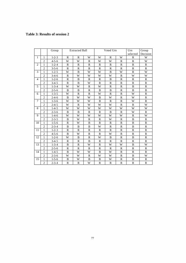
77
Table 3: Results of session 2
Group Extracted Ball Voted Urn Urn
selected Group Decision
1 1-2-3 R R W W R W R W 1 2 4-5-6 W W R W W R R W 1 1-2-4 R R R R R R R R 2 2 3-5-6 R R R R R R R R 1 1-2-5 W B W W B W R W 3 2 3-4-6 R W W W W R W W 1 1-2-6 R B R R B R R R 4 2 3-4-5 R B W R R R R R 1 1-3-4 W W R W R R B R 5 2 2-5-6 B B R B B R B B 1 1-3-5 W R R W R R W R 6 2 2-4-6 B W W B W R W R 1 1-3-6 W W W B R R W R 7 2 2-4-5 W R W W W R R W 1 1-4-5 W W W W W W W W 8 2 2-3-6 B B R R B R W R 1 1-4-6 W W W W W W R W 9 2 2-3-5 B W R R W R B R 1 1-5-6 R W B R R R B R 10 2 2-3-4 B B B W R R B R 1 1-2-3 R R R R R R R R 11 2 4-5-6 B W R R W R R R 1 1-2-6 W B R W B R B R 12 2 3-4-5 R R B R R R R R 1 1-3-4 B R W R W W B W 13 2 2-5-6 R R R R R R R R 1 1-4-5 B W W B W R R R 14 2 2-3-6 W W R W W R B W 1 1-5-6 B W B B W R B R 15 2 2-3-4 R R W R R R R R

78
Table 4: Results of session 3
Group Extracted Ball Voted Urn Urn selected
Group Decision
1 1-2-3 W W R W W R B W 1 2 4-5-6 B W W R W W W W 1 1-2-4 R R W R R W W R 2 2 3-5-6 R W R R W R R R 1 1-2-5 R W R R W R R R 3 2 3-4-6 W B R R R R R R 1 1-2-6 R R R R R R R R 4 2 3-4-5 B W W R W W B W 1 1-3-4 R W R W W R R W 5 2 2-5-6 W W W W W W W W 1 1-3-5 R R B R R B W R 6 2 2-4-6 W B W W R W W W 1 1-3-6 B B W W B W W W 7 2 2-4-5 W R W R R W R R 1 1-4-5 W W W R R W W R 8 2 2-3-6 B B R B B R B B 1 1-4-6 R R R R R R R R 9 2 2-3-5 R B R R R R R R 1 1-5-6 R W B R W R R R 10 2 2-3-4 W R R W R R R R 1 1-2-3 B B R W B R B R 11 2 4-5-6 B R W B R W W R 1 1-2-6 B B R B B R B B 12 2 3-4-5 R R W R R W R R 1 1-3-4 W B W W B W W W 13 2 2-5-6 W R R W R R R R 1 1-4-5 B B W B B W W B 14 2 2-3-6 R W R R W R W R 1 1-5-6 R R B R R R R R 15 2 2-3-4 R R R R R R R R

79
Table 5: Results of session 4
Group Extracted Ball Voted Urn Urn selected
Group Decision
1 1-2-3 R B W R B W W R 1 2 4-5-6 R R R R R R R R 1 1-2-4 B R W R R W R R 2 2 3-5-6 R R R R R R R R 1 1-2-5 R R B W R B R R 3 2 3-4-6 R W R R W R R R 1 1-2-6 R R R R R R R R 4 2 3-4-5 R B R R B R R R 1 1-3-4 R R R R R R R R 5 2 2-5-6 B B B R B R B R 1 1-3-5 R W B B W R R R 6 2 2-4-6 B B R R B R R R 1 1-3-6 R R W W R W R W 7 2 2-4-5 R R R R R R R R 1 1-4-5 R W W R W W W W 8 2 2-3-6 B B B R B R B R 1 1-4-6 R B B R B R W R 9 2 2-3-5 B R R R R R R R 1 1-5-6 R B R R B R R R 10 2 2-3-4 W W B W W B R W 1 1-2-3 R W W R R W W R 11 2 4-5-6 R B B R B B R B 1 1-2-6 R R W B R W R R 12 2 3-4-5 W B R W B R B R 1 1-3-4 R W R R W R R R 13 2 2-5-6 B W B R W R B R 1 1-4-5 R W R R W R R R 14 2 2-3-6 W W W W W R W W 1 1-5-6 B R B B R R B R 15 2 2-3-4 R R R R R R R R

80
References
Condorcet, Marquis de (1785), Essai sur l’Application de l’Analyse a la Probabilite des Decisions Rendues a la Probabilite des Voix, Imprimerie royale, Paris; Feddersen, T. and W. Pesendorfer (1998), Convicting the Innocent: The Inferiority of Unanimous Jury Verdicts under Strategic Voting, American Political Science Review 92, No 1, 23-35; Guarnaschelli, S., McKelvey R. and T. Palfrey (2000), An Experimental Study of Jury Decision Rules, American Political Science Review 94, No. 2, 407-22; Ladha, K., Miller G. and J. Oppenheimer (1996), Information Aggregation by Majority Rule: Theory and Experiments, University of Maryland; McKelvey, R., and T. Palfrey (1995), Quantal Response Equilibria for Normal Form Games, Games and Economic Behavior, 10, 6-38; McKelvey, R., and T. Palfrey (1998), Quantal Response Equilibria for Extensive Form Games, Experimental Economics, 1, 9-41; Rata, C. (2002), Strategic Aspects of Info rmation Aggregation by Plurality Rule, Universitat Autònoma de Barcelona, mimeo.