NEW LEARNING ALGORITHM BASED HIDDEN MARKOV MODEL

(HMM) AS STOCHASTIC MODELLING FOR PATTERN

CLASSIFICATION

MALARVILI BALAKRISHNAN

TING CHEE MING

SHEIKH HUSSAIN SHAIKH SALLEH

RESEARCH VOTE NO:

78208

Faculty of Biomedical Engineering and Health Science

Universiti Teknologi Malaysia

SEPTEMBER 2009

VOT 78208

ii

ABSTRACT

This study investigates the use discriminative training methods of minimum

classification error (MCE) to estimate the parameter of hidden Markov model

(HMM). The conventional training of HMM is based on the maximum likelihood

estimation (MLE) which aims to model the true probabilistic distribution of the data

in term of maximizing the likelihood. This requires sufficient training data and

correct choice of probabilistic models, which in reality hardly achievable. The

insufficient training data and incorrect modeling assumption of HMM often yield an

incorrect and unreliable model. Instead of learning the true distribution, the MCE

based training targeted to minimizing the probability of error is used to obtain

optimal Bayes classification. The central idea of MCE based training is to define a

continuous, differentiable loss function to approximate the actual performance error

rate. Gradient based optimization methods can be used to minimize this loss. In this

study the first order online generalized probabilistic descent is used as optimization

methods. The continuous density HMM is used as the classifier structure in the MCE

framework. The MCE based training is evaluated on speaker-independent Malay

isolated digit recognition. The MCE training achieves the classification accuracy of

96.4% compared to 96.1% of using MLE with small improvement rate of 0.31%. The

small vocabulary is unable to reflect the performance comparison of the two methods,

the MLE training given sufficient training data is sufficient to provide optimal

classification accuracy. Future work will extend the evaluation on difficult

classification task such as phoneme classification, to better access the discriminative

ability of the both methods.

iii

ABSTRAK

Kajian ini mengaji penggunaan cara perlatihan kesilapan klasifikasi minimal

(minimum classification error (MCE)) dalam penganggaran parameter model Makov

tersembunyi (hidden Markov model (HMM)). Cara konvensional dalam perlatihan

HMM adalah berdasarkan pengganggaran kebarangkalian maximum yang bertujuan

memodelkan taburan kebarangkalian yang tepat dalam memaximakan

kebarangkalian. Ini memerlukan data latihan yang mencukupi dan pilihan model

kebarangkalian yang betul, dimana susah dicapai. Data latihan yang tidak mencukupi

dan model yang tidak tepat selalu menhasilkan model yang tidak tepat. Berbeza

daripada membelajar taburan yang benar, latihan MCE bertujuan meminimumkan

kesilapan kebarangkalian untuk mencapai klasifikasi Bayes yang optima. Idea di

bawah latihan MCE adalah untuk mendefinisikan satu fungsi loss yang berterusan

dan boleh dibezakan untuk menganggarkan kadar kesilapan yang benar. Teknik

optimasi gradient boleh digunakan untuk meminimumkan fungsi ini. Online

generalized probabilistic descent digunakan sebagai teknik optimasi. Model density

berterusan (continuous density HMM) digunakan sebagai struktur klasifikasi dalam

rangka MCE. MCE diuji dengan penutur-bebas pegecaman digit Melayu berasingan.

MCE mencapai ketepatan klasifikasi 96.4% berbanding dengan 96.1% dengan

mengunakan MLE, dengan peningkatan yang kecil 0.31%. Vokabolari yang kecil

tidak berupaya memaparkan perbandingan antara dua teknik. Latihan MLE jika

diberi data latihan yang mencukupi akan memberikn ketrpatan klasifikasi yang

optima. Kerja masa depan akan menggunakan penilaian dengan mengunakan

klasifikasi phoneme yang lebih mencabar untuk mendapatkan keupayaan

diskriminasi antara dua teknik.

iv

TABLE OF CONTENTS

CHAPTER TITLE PAGE

TITLE PAGE i

ABSTRACT ii

ABSTRAK iii

TABLE OF CONTENTS iv

LIST OF TABLES vi

LIST OF SYMBOLS vii

1 INTRODUCTION 1

1.1 Introduction and Motivation 1

1.3 Objectives of the Research 2

1.4 Scope of Research 3

2 MINIMUM CLASSIFICATION ERROR

BASED TRAINING OF HIDDEN MARKOV

MODELS 4

2.1 Introduction 4

2.2 Bayes Decision Theory & MCE/GPD 5

2.3 MCE based Optimization 6

2.3.1 Formulation of MCE Loss Function 6

2.3.1.1 Discriminant Function 7

2.3.1.2 Misclassification Measure 7

2.3.1.3 MCE Loss 8

v

2.3.2 Optimization Methods 8

2.4 MCE Training of HMMs 9

2.4.1 HMM as Discriminant Function 10

2.4.2 MCE Loss & Optimization 11

2.4.3 Derivation of MCE Gradients 11

3 EXPERIMENTAL EVALUATION 15

3.1 Task and Database 15

3.2 Experimental Setup 15

3.3 Experimental Results 16

4 CONCLUSIONS & FUTURE WORKS 17

vi

LIST OF TABLES

TABLES NO. TITLE PAGE

3.1 Number of misclassified tokens of each digit for

MLE and MCE training on test set evaluation. 16

vii

LIST OF SYMBOLS

HMM - Hidden Markov Model

MCE - Minimum classification error

MFCC - Mel-Frequency Cepstral Coefficients

MLE - Maximum Likelihood Estimation

MMI - Maximum mutual information

CDHMM - Continuous Density Hidden Markov Model

- HMM Model

Tx1 - Sequence of acoustic feature vectors.

1

CHAPTER 1

INTRODUCTION

1.1 Background and Motivation

Hidden Markov models (HMMs) have been widely studied as statistical pattern

classification since decades. HMM has been widely used in various applications such as

speech recognition, image recognition, bioinformatics, and others. HMM is a doubly

stochastic process which models the temporal structure of sequential pattern through its

Markov chain, and models the probabilistic nature of the observation via its probability

density function assigned with each state. The advantages of HMM lie on its established

statistical framework and working well practically. The conventional parameter

estimation of HMM are based on maximum likelihood estimation (MLE) which aims at

optimal statistical distribution fitting in term of increasing the HMM likelihood. The

optimality of this training criterion assumes sufficient training data and correct choice of

distribution with enough parameters [Chao et al 1992], which will yield a classifier close

to the optimal Bayes classifier. However, in reality, the training data is limited to

reliably train model with many parameters. Furthermore, the underlying assumptions of

HMM often incorrectly model the real probabilistic nature of sequential data [McDermott

1997].

This deficiency in the conventional training methods motivates the use of

discriminative training which aims to minimizing the probability of classification error

2

instead of estimating the true probability distribution. Discriminative training methods

such as maximum mutual information (MMI) [Bahl et al 1986] and minimum

classification error (MCE) [Juang et al 1997; McDermott 1997] have been proposed.

MCE is more directly aims to minimizing the recognition error, compared to MMI

which targeted at optimizing the mutual information [McDermott 1997]. Use of MCE in

HMM training is the main focus in this research.

The MCE criterion is more directly aimed at attaining the optimal Bayes

classification. The central idea of MCE based training is to define a continuous,

differentiable loss function to approximate the actual performance error rate. Gradient

based optimization methods can be used to minimize this loss. This approach allows but

does not require the use of explicit probabilistic models. Furthermore, MCE training

does not involve the estimation of probability distributions, which is difficult to perform

reliably. The MCE overcome the problem of using incorrect probabilistic model, since

the MCE aims at reducing the classification error, and not in learning the true

probabilistic distribution of the data. In contrast, the MLE will usually fail to yield a

minimum risk classifier despite sufficient training data is available. Learning to separate

pattern classes optimally is not necessarily the same problem as learning to model the

true probability distribution for each class [McDermott 1997].

1.2 Objectives of the Research

The main objective of this study is to investigate MCE based optimization

methods for parameter estimation of HMM. To achieve the main objective, several sub-

objectives are addressed in this thesis as following:

(1) To investigate the principle and framework of MCE based optimization.

(2) To investigate the use of the MCE framework in the training of HMM.

3

1.3 Scope of Research

The scope of task and the scope of approaches used in this thesis are defined as

follows:

(1) The MCE training of HMM is evaluated on isolated Malay digit

recognition.

(2) The techniques and approaches used in solving the tasks are as follow:

(a) Left-to-right continuous density hidden Markov model (CDHMM)

with Gaussian mixture densities (Rabiner 1989)is used as

classifier models and the likelihood of the optimal path serves as

the discriminant function in the MCE framework.

(b) Online Probabilistic descent (GPD) is used the gradient based

optimization to minimizing the MCE loss.

(c) Mel-frequency cepstral coefficient (MFCC) are used for feature

extraction.

4

CHAPTER 2

MINIMUM CLASSIFICATION ERROR BASED TRAINING OF HIDDEN MARKOV MODELS

2.1 Introduction

The minimum classification error (MCE) framework has been proposed for

discriminative training, which directly minimize the recognition error rate. This chapter

discusses the theoretical foundation and formulation of the MCE based optimization. In

this report, hidden Markov models are estimated using MCE based training.[Chao et al

1992; Juang et al 1997] The chapter firstly discusses the Bayes decision theory as a

motivation of formulating MCE method. Next the loss function of MCE is formulated

and optimized using Generalized Probabilistic Descent (GPD) [Katagiri et al. 1990;

Juang & Katagiri 1992]. The final section describes the application of MCE in training

continuous density hidden Markov models (CDHMM). The description in this chapter is

mainly based on [McDermott 1997; Juang et al 1997; Chao et al 1992; McDermott et al

2007].

5

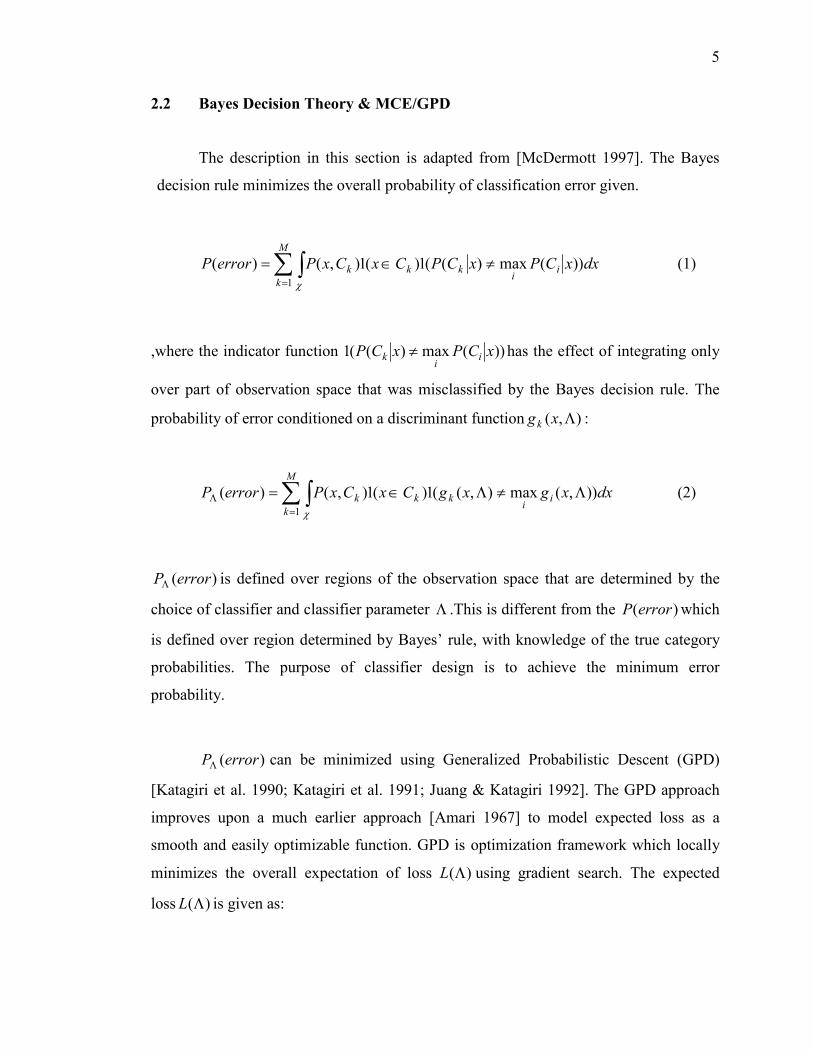
2.2 Bayes Decision Theory & MCE/GPD

The description in this section is adapted from [McDermott 1997]. The Bayes

decision rule minimizes the overall probability of classification error given.

dxxCPxCPCxCxPerrorP ii

kk

M

kk ))(max)((1)(1),()(

1

≠∈=∑∫= χ

(1)

,where the indicator function ))(max)((1 xCPxCP ii

k ≠ has the effect of integrating only

over part of observation space that was misclassified by the Bayes decision rule. The

probability of error conditioned on a discriminant function ),( Λxg k :

dxxgxgCxCxPerrorP ii

kk

M

kk )),(max),((1)(1),()(

1

Λ≠Λ∈=∑∫=

Λ

χ

(2)

)(errorPΛ is defined over regions of the observation space that are determined by the

choice of classifier and classifier parameter Λ .This is different from the )(errorP which

is defined over region determined by Bayes’ rule, with knowledge of the true category

probabilities. The purpose of classifier design is to achieve the minimum error

probability.

)(errorPΛ can be minimized using Generalized Probabilistic Descent (GPD)

[Katagiri et al. 1990; Katagiri et al. 1991; Juang & Katagiri 1992]. The GPD approach

improves upon a much earlier approach [Amari 1967] to model expected loss as a

smooth and easily optimizable function. GPD is optimization framework which locally

minimizes the overall expectation of loss )(ΛL using gradient search. The expected

loss )(ΛL is given as:

6

dxCxpxCPxEL kk

M

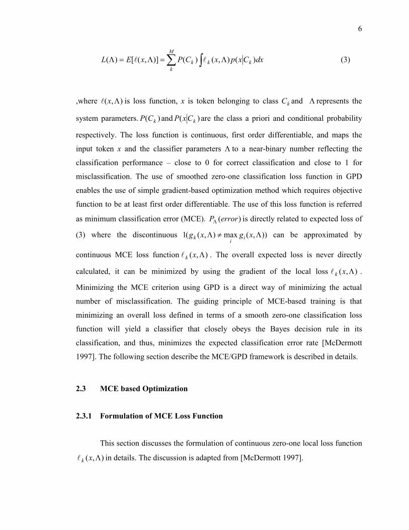
kk )(),()()],([)( ∫∑ Λ=Λ=Λ ll (3)

,where ),( Λxl is loss function, x is token belonging to class kC and Λ represents the

system parameters. )( kCP and )( kCxP are the class a priori and conditional probability

respectively. The loss function is continuous, first order differentiable, and maps the

input token x and the classifier parameters Λ to a near-binary number reflecting the

classification performance – close to 0 for correct classification and close to 1 for

misclassification. The use of smoothed zero-one classification loss function in GPD

enables the use of simple gradient-based optimization method which requires objective

function to be at least first order differentiable. The use of this loss function is referred

as minimum classification error (MCE). )(errorPΛ is directly related to expected loss of

(3) where the discontinuous )),(max),((1 Λ≠Λ xgxg ii

k can be approximated by

continuous MCE loss function ),( Λxkl . The overall expected loss is never directly

calculated, it can be minimized by using the gradient of the local loss ),( Λxkl .

Minimizing the MCE criterion using GPD is a direct way of minimizing the actual

number of misclassification. The guiding principle of MCE-based training is that

minimizing an overall loss defined in terms of a smooth zero-one classification loss

function will yield a classifier that closely obeys the Bayes decision rule in its

classification, and thus, minimizes the expected classification error rate [McDermott

1997]. The following section describe the MCE/GPD framework is described in details.

2.3 MCE based Optimization

2.3.1 Formulation of MCE Loss Function

This section discusses the formulation of continuous zero-one local loss function

),( Λxkl in details. The discussion is adapted from [McDermott 1997].

7

2.3.1.1 Discriminant Function

The discriminant function ),( Λxg k is defined to reflect the extent to which the

token x belongs to the class kC . The discriminant function depends on the choice of

classifier structure. For feed-forward MLP, the discriminant function will be output

value of the MLP given the input. For hidden Markov model, the discriminant function

will be the probability of generating the pattern of observation sequence given the model.

Assuming the greater discriminant function value indicate a better match, the decision

rule is given as:

.),(),( jkallforxgxgCDecide kjj ≠Λ>Λ (4)

2.3.1.2 Misclassification Measure

The MCE misclassification measure compares the discriminant function value

for the correct class and incorrect class. One way to formulate the misclassification

measure ),( Λxd k for token x of class kC is given as [McDermott 1997]

ψψ

1

),(1

1),(),(

Λ

−+Λ−=Λ ∑

≠kjjkk xg

Mxgxd . (5)

,where M is the number of classes. This misclassification measure is a continuous

function of the classifier parameters and attempts to emulate the decision rule.

0),( >Λxd k implies misclassification and 0),( ≤Λxd k means correct decision [Juang

et al 1997]. When ψ approach∞ , the term in the bracket is approximately the value of

the discriminant function of the best incorrect class ),(max Λ≠ xg jkjj , which is used in

this study.

8

2.3.1.3 MCE Loss

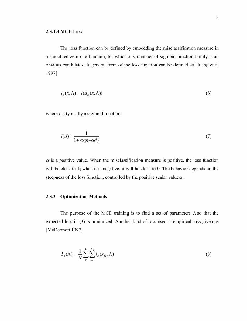
The loss function can be defined by embedding the misclassification measure in

a smoothed zero-one function, for which any member of sigmoid function family is an

obvious candidates. A general form of the loss function can be defined as [Juang et al

1997]

)),((),( Λ=Λ xdlxl kk (6)

where l is typically a sigmoid function

)exp(1

1)(

ddl

α−+= (7)

α is a positive value. When the misclassification measure is positive, the loss function

will be close to 1; when it is negative, it will be close to 0. The behavior depends on the

steepness of the loss function, controlled by the positive scalar valueα .

2.3.2 Optimization Methods

The purpose of the MCE training is to find a set of parameters Λ so that the

expected loss in (3) is minimized. Another kind of loss used is empirical loss given as

[McDermott 1997]

),(1

)(1

1 Λ=Λ ∑∑=

ik

M

k

N

ik xl

NL

k

(8)

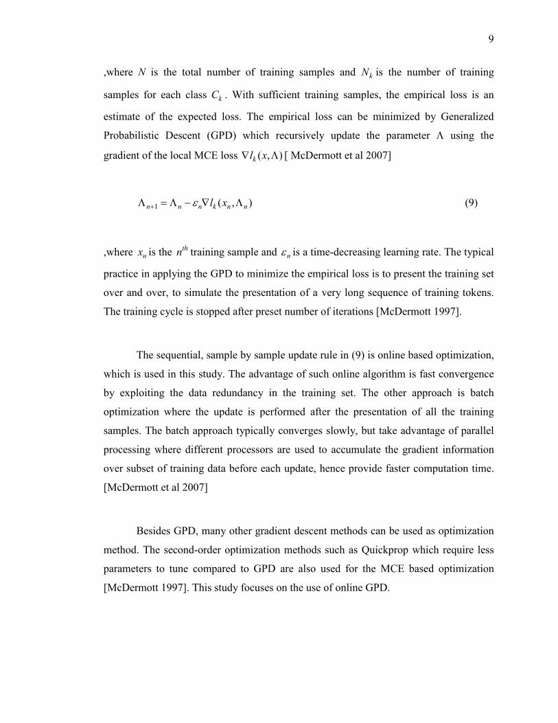
9

,where N is the total number of training samples and kN is the number of training

samples for each class kC . With sufficient training samples, the empirical loss is an

estimate of the expected loss. The empirical loss can be minimized by Generalized

Probabilistic Descent (GPD) which recursively update the parameter Λ using the

gradient of the local MCE loss ),( Λ∇ xlk [ McDermott et al 2007]

),(1 nnknnn xl Λ∇−Λ=Λ + ε (9)

,where nx is the thn training sample and nε is a time-decreasing learning rate. The typical

practice in applying the GPD to minimize the empirical loss is to present the training set

over and over, to simulate the presentation of a very long sequence of training tokens.

The training cycle is stopped after preset number of iterations [McDermott 1997].

The sequential, sample by sample update rule in (9) is online based optimization,

which is used in this study. The advantage of such online algorithm is fast convergence

by exploiting the data redundancy in the training set. The other approach is batch

optimization where the update is performed after the presentation of all the training

samples. The batch approach typically converges slowly, but take advantage of parallel

processing where different processors are used to accumulate the gradient information

over subset of training data before each update, hence provide faster computation time.

[McDermott et al 2007]

Besides GPD, many other gradient descent methods can be used as optimization

method. The second-order optimization methods such as Quickprop which require less

parameters to tune compared to GPD are also used for the MCE based optimization

[McDermott 1997]. This study focuses on the use of online GPD.

10

2.4 MCE Training of HMMs

MCE training have been used for parameter estimation of hidden Markov models

[Chao et al 1992]. This section discusses the application of MCE framework to HMM

optimization. The discussions in these sections follow [McDermott 1997].

2.4.1 HMM as Discriminant Function

Details of the hidden Markov modeling refer to [Rabiner 1989]. In HMMs, The

observation probability density function of observation tx at time t, given the mean

vectors is,µ and covariance matrices is,Σ of an HMM state s, is typically a Gaussian

mixture density:

),,,()( ,,1

, isist

I

iists xNcxb Σ=∑

=

µ (10)

,where I is the number of mixture components in state s and isc , are mixture weights

satisfying the constraint:

.11

, =∑=

I

iisc (11)

),,( ,, isistxN Σµ is the multivariate Gaussian density of d-dimensional observation vector

tx given as

)).()(21

exp()2(

1),,( 1

2/12/µµ

πµ −Σ−−

Σ=Σ − xxxN T

D (12)

11

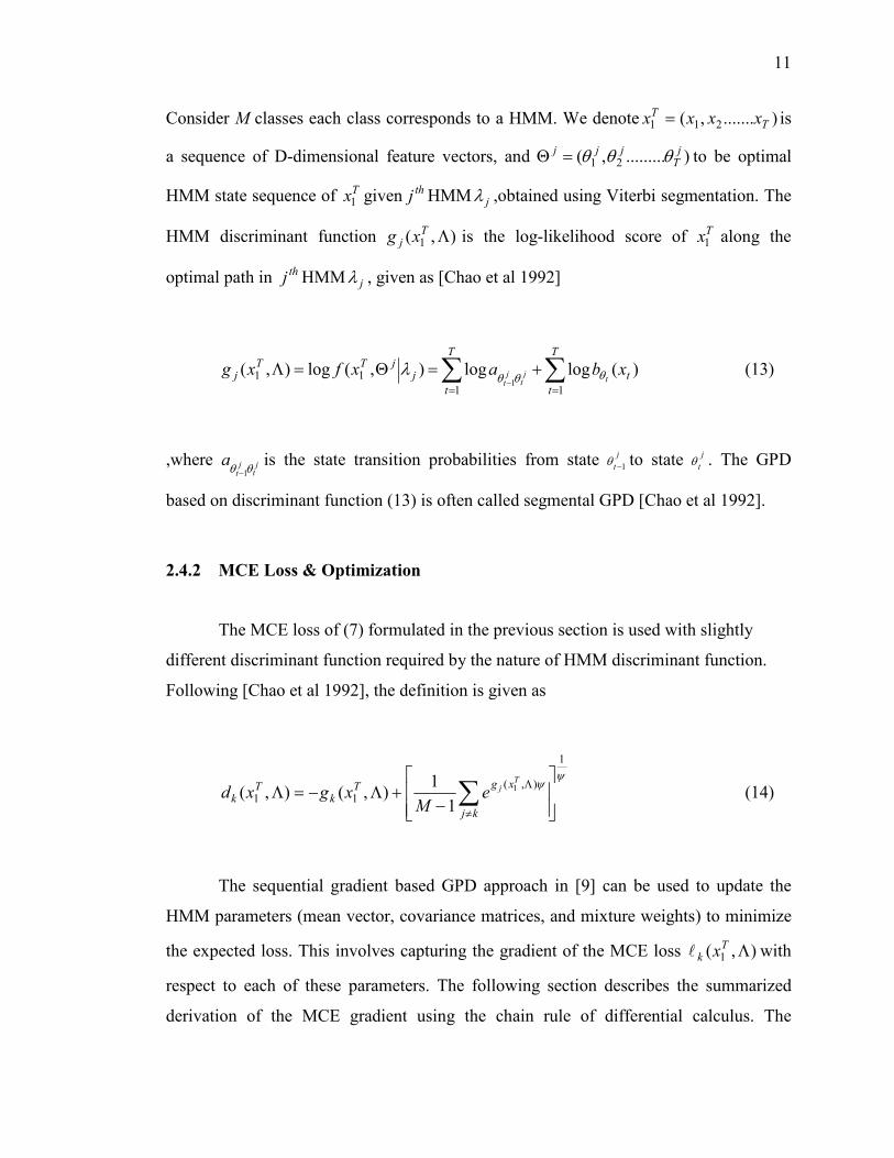
Consider M classes each class corresponds to a HMM. We denote ).......,( 211 TT xxxx = is

a sequence of D-dimensional feature vectors, and ).........,( 21jT

jjj θθθ=Θ to be optimal

HMM state sequence of Tx1 giventhj HMM jλ ,obtained using Viterbi segmentation. The

HMM discriminant function ),( 1 ΛTj xg is the log-likelihood score of Tx1 along the

optimal path in thj HMM jλ , given as [Chao et al 1992]

)(loglog),(log),(11

111

t

T

t

T

tj

jTTj xbaxfxg

tjt

jt

∑∑==

+=Θ=Λ−

θθθλ (13)

,where jt

jt

a θθ 1−is the state transition probabilities from state j

t 1−θ to state jtθ . The GPD

based on discriminant function (13) is often called segmental GPD [Chao et al 1992].

2.4.2 MCE Loss & Optimization

The MCE loss of (7) formulated in the previous section is used with slightly

different discriminant function required by the nature of HMM discriminant function.

Following [Chao et al 1992], the definition is given as

ψψ

1

),(11

1

11

),(),(

−+Λ−=Λ ∑

≠

Λ

kj

xgTk

Tk

Tje

Mxgxd (14)

The sequential gradient based GPD approach in [9] can be used to update the

HMM parameters (mean vector, covariance matrices, and mixture weights) to minimize

the expected loss. This involves capturing the gradient of the MCE loss ),( 1 ΛTk xl with

respect to each of these parameters. The following section describes the summarized

derivation of the MCE gradient using the chain rule of differential calculus. The

12

discussion is adapted directly from the Appendix of [McDermott et al 2007] with some

modifications.

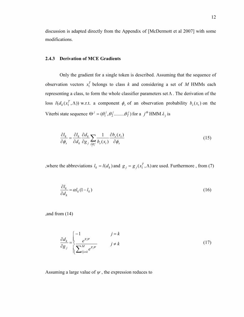
2.4.3 Derivation of MCE Gradients

Only the gradient for a single token is described. Assuming that the sequence of

observation vectors Tx1 belongs to class k and considering a set of M HMMs each

representing a class, to form the whole classifier parameters setΛ . The derivation of the

loss )),(( 1 ΛTk xdl w.r.t. a component sφ of an observation probability )( ts xb on the

Viterbi state sequence ).........,( 21jT

jjj θθθ=Θ for a thj HMM jλ is

s

ts

t tsj

k

k

k

s

k xbxbg

ddll

jt

φφθ

∂∂

∂∂

∂∂

=∂∂

∑)(

)(1

(15)

,where the abbreviations )( kk dll = and ),( 1 Λ= Tjj xgg are used. Furthermore , from (7)

)1( kkk

k lldl

−=∂∂

α (16)

,and from (14)

≠

=−

=∂∂

∑ ≠

kje

ekj

gd

M

kii

g

g

j

k

j

j

ψ

ψ1

(17)

Assuming a large value of ψ , the expression reduces to

13

=

=−

=∂∂

≠

otherwise

gj

kj

gd

jkiij

k

,0

maxarg,1

,1

(18)

In this case, the derivatives only exist for the correct and best incorrect class.

In practice, s

klφ∂∂

is accumulated along jΘ for each model jλ , adding to the partial

derivative of the loss function with respect to each component sφ , which potentially

ranges over all mixture weights, mean vector, and covariance components.

Now, the rest of the partial derivatives can be specified. The Gaussian mixture

density has been defined in (10). Using the abbreviation ),,()( ,,, isisttis xNxN Σ= µ ,the

partial derivatives of )( ts xb with respect to the transformed mixture weights

isis cc ,, log= , mean vector component dis ,,µ , and transformed inverse covariance

component 1,,,, log −= disdis σσ are respectively,

)()(

,,,

tisisis

ts xNccxb

=∂∂

))(()(

,,,,,,,

disdttisisdis

ts xxNcxb

µµ

−=∂∂

))(1)(()( 2

,,,2

,,,,

,,disdttisis

dis

ts xexNcxb dis µ

σσ −−=

∂∂

(19)

14

These term are used to expand s

ts xbφ∂

∂ )(in (15). Adaptation of isc , ,followed by the back

transformation )exp( ,, isis cc = during parameter updating, enforces the constraint that the

mixture weights must stay positive. The additional constraint that the mixture weights

must sum to one can be maintained simply by normalizing the weights after each

iteration of MCE. Adaptation of the transformed inverse covariance term dis ,,σ results in

greater numerical accuracy than adaptation of dis ,,σ itself. Finally, in the interest of

numerical stability, a division by 2,, disσ term has been dropped from the true derivative

for the mean [McDermott et al 2007].

15

CHAPTER 3

EXPERIMENTAL EVALUATION

3.1 Task and Database

The MCE/GPD framework is evaluated on speaker-independent Malay isolated

digit recognition. The continuous density HMM (CDHMM) is used for discriminant

function. The recognition vocabulary consists of 9 Malay digit (‘SATU’, ‘DUA’,

‘TIGA’, ‘EMPAT’, ‘LIMA’, ‘ENAM’, ‘TUJUH’, ‘ LAPAN’, ‘SEMBILAN’). The

database consists of 100 speaker each recorded 5 tokens for each digit. The training set

consists of 20 speaker and the remaining 80 speakers as test set which consists of 3600

digit tokens.

3.2 Experimental Setup

The speech is sampled at 16KHz. The speech signal is represented by a sequence

of 12 dimensional vector of Mel-Frequency Cepstral Co-efficients (MFCCs). Each

Malay digit is modeled by a 5-state CDHMM with 4 Gaussian components. The models

are trained based on conventional maximum likelihood estimation (MLE) using 8

iterations of segmental K-mean algorithm [Rabiner 1989]. These trained models are

used for the initialization of the online MCE/GPD training. The α is empically set as

0.005 and the learning rate as 0.05. For preliminary study, only 1 iteration of MCE

update is run through the whole training set. The Viterbi decoding is used for

16

recognition. [Rabiner 1989]. Comparison in term of recognition performance is made

between the MLE and MCE based training.

3.3 Experimental Results

Table 1 shows the number of misclassified tokens of each digit for the MLE and

MCE based training. The MCE training increases the classification accuracy of 96.1%

when using MLE, to 96.4% with small improvement rate of 0.31%. The small

vocabulary is unable to reflect the performance comparison of the two methods, the

MLE training given sufficient training data is sufficient to provide optimal classification

accuracy. Future work will extend the evaluation on difficult classification task such as

phoneme classification, to better access the discriminative ability of the both methods.

Table 1. Number of misclassified tokens of each digit for MLE and MCE

training on test set evaluation.

MLE MCE

SATU 6 6

DUA 40 34

TIGA 21 20

EMPAT 4 2

LIMA 17 18

ENAM 8 8

TUJUH 26 24

LAPAN 6 9

SEMBILAN 12 7

Total 140 128

17

CHAPTER 4

CONCLUSIONS & FUTURE WORKS

The MCE based training of HMM has been described and evaluated on speaker-

independent Malay isolated digit recognition. The MCE training achieves the better

classification accuracy of 96.4% compared to 96.1% of using MLE with small

improvement rate of 0.31%. The number of token misclassification using MCE is lower

than using MLE, which shows that MCE provide better discriminative ability. However,

the small vocabulary is unable to reflect the performance comparison of the two methods,

the MLE training given sufficient training data is sufficient to provide optimal

classification accuracy. Future work will extend the evaluation on difficult classification

task such as phoneme classification, to better access the discriminative ability of the

both methods.

Other gradient based optimization methods such as second order Quick-prop can

be used for MCE training framework [McDermott 1997]. Besides, the MCE

discriminative training can be extended to the large vocabulary continuous speech

applications[McDermott et al 2007]. Future work will investigate the effect of learning

rate, number of training iterations, and alpha value of the MCE loss to the recognition

performance.

18

REFERENCES

McDermott E. et. al. (2007). “Discriminative Training for Large-Vocabulary Speech

Recognition Using Minimum Classification Error,” IEEE Trans. on Audio, Speech, and

Language Processing, vol. 15, No. 1, pp. 203-223.

Juang B. H. et. al., (1997). “Minimum Classification Error Rate Methods for speech

recognition,” IEEE Trans. on Speech and Audio Processing, vol. 5, No. 3, pp. 257-265.

Chou W. et. al., (1992). “Segmental GPD Training of HMM Based Speech Recognizer,” IEEE

International Conference on Acoustics, Speech, and Signal Processing, vol. 1, pp. 473-476.

McDermott E. (1997), “Discriminative Training for Speech Recognition,” PhD Thesis, Waseda

University.

Bahl et. al., (1986). “Maximum Mutual Information Estimation of Hidden Markov Parameters

for Speech Recognition,” IEEE International Conference on Acoustics, Speech, and Signal

Processing.

Kapadia S. (1998), “Discriminative Training of Hidden Markov Models,” PhD Thesis,

University of Cambridge.

Rabiner S. (1989) “A tutorial on hidden Markov models and selected applications in Speech

Recognition,” Proc. of IEEE, Vol. 77, No. 2, pp. 257-286.

19

Katagiri et al. (1991). “New Discriminative Training Algorithm Based on the Generalized

Descent Method,” IEEE Workshop on Neural Networks for Signal Procesing, pp. 299-308, 1991.

Katagiri et al. (1990). “A Genralized Probabilistic Descent Method,” Proc. of the Acoustical

Society of Japan, pp. 141-142.

Juang B. H. & Katagiri. (1992). “Discriminative Learning for Minimum Error Classification,”

IEEE Trans. on Signal Processing, vol. 40, no. 12 pp. 3043-3053.

Amari S. (1967). “A Theory of Adaptive Pattern Classifiers,” IEEE Trans. on Electronics

Computer,” vol. EC-16, no. 3, pp. 299-307.