Von Neumann Algebras.

Vaughan F.R. Jones 1

November 13, 2015

1Supported in part by NSF Grant DMS93–22675, the Marsden fund UOA520,and the Swiss National Science Foundation.

2

Chapter 1

Introduction.

The purpose of these notes is to provide a rapid introduction to von Neumannalgebras which gets to the examples and active topics with a minimum oftechnical baggage. In this sense it is opposite in spirit from the treatises ofDixmier [], Takesaki[], Pedersen[], Kadison-Ringrose[], Stratila-Zsido[]. Thephilosophy is to lavish attention on a few key results and examples, and weprefer to make simplifying assumptions rather than go for the most generalcase. Thus we do not hesitate to give several proofs of a single result, or repeatan argument with different hypotheses. The notes are built around semester-long courses given at UC Berkeley and Vanderbilt though they contain morematerial than could be taught in a single semester.

The notes are informal and the exercises are an integral part of the ex-position. These exercises are vital and mostly intended to be easy.

3

4

Chapter 2

Background and Prerequisites

2.1 Hilbert SpaceA Hilbert Space is a complex vector spaceH with inner product 〈, 〉 : HxH →C which is linear in the first variable, satisfies 〈ξ, η〉 = 〈η, ξ〉, is positivedefinite, i.e. 〈ξ, ξ〉 > 0 for ξ 6= 0, and is complete for the norm defined by test

||ξ|| =√〈ξ, ξ〉.

Exercise 2.1.1. Prove the parallelogram identity :

||ξ − η||2 + ||ξ + η||2 = 2(||ξ||2 + ||η||2)

and the Cauchy-Schwartz inequality:

|〈ξ, η〉| ≤ ||ξ|| ||η||.

Theorem 2.1.2. If C is a closed convex subset of H and ξ is any vector inH, there is a unique η ∈ C which minimizes the distance from ξ to C, i.e.||ξ − η′|| ≤ ||ξ − η|| ∀η′ ∈ C.

Proof. This is basically a result in plane geometry.Uniqueness is clear—if two vectors η and η′ in C minimized the distance

to ξ, then ξ, η and η′ lie in a (real) plane so any vector on the line segmentbetween η and η′ would be strictly closer to ξ.

To prove existence, let d be the distance from C to ξ and choose a sequenceηn ∈ C with ||ηn − ξ|| < d + 1/2n. For each n, the vectors ξ, ηn and ηn+1

define a plane. Geometrically it is clear that, if ηn and ηn+1 were not close,some point on the line segment between them would be closer than d to ξ.Formally, use the parallelogram identity:

||ξ − ηn + ηn+1

2||2 = ||ξ − ηn

2+ξ − ηn+1

2||2

5

= 2(||ξ − ηn2||2 + ||ξ − ηn+1

2||2 − 1/8||ηn − ηn+1||2)

≤ (d+ 1/2n)2 − 1/4||ηn − ηn+1||2

Thus there is a constant K such that ||ηn−ηn+1||2 < K/2n or ||ξ− ηn+ηn+1

2||2

would be less than d2.Thus (ηn) is Cauchy, its limit is in C and has distance d from ξ.

Exercise 2.1.3. If φ ∈ H∗ (the Banach-space dual of H consisting of allcontinuous linear functionals from H to C), kerφ is a closed convex subsetof H. Show how to choose a vector ξφ orthogonal to kerφ with φ(η) = 〈ξφ, η〉and so that φ 7→ ξφ is a conjugate-linear isomorphism from H∗ onto H.

We will be especially concerned with separable Hilbert Spaces where thereis an orthonormal basis, i.e. a sequence ξ1, ξ2, ξ3, ... of unit vectors with〈ξi, ξj〉 = 0 for i 6= j and such that 0 is the only element of H orthogonal toall the ξi.

We will use the abbreviation ONB for orthonormal basis.

Exercise 2.1.4. Show that an ONB always exists (e.g. Gram-Schmidt) andthat if ξi is an ONB for H then the linear span of the ξi is dense in H.

A trivial but useful observation. If H and K are Hilbert spaces withvectors ξi ∈ H and ψk ∈ K respectively then if

〈ξi, ξj〉 = 〈ψi, ψj〉 ∀i, j

then the map ξi 7→ ψi extends to a linear 〈, 〉-preserving bijection from theclosure of the subspace spanned by the ξi to the closure of the subspacespanned by the ψi.

A linear map (operator) a : H → K is said to be bounded if there is anumber K with ||aξ|| ≤ K||ξ|| ∀ξ ∈ H. The infimum of all such K is calledthe norm of a, written ||a||. The set of all bounded operators from H to Kis written B(H,K) and if H = K we use B(H). Boundedness of an operatoris equivalent to continuity.

To every bounded operator a between Hilbert spacesH and K, by exercise2.1.3 there is another, a∗, between K and H, called the adjoint of a which isdefined by the formula 〈aξ, η〉 = 〈ξ, a∗η〉.

Exercise 2.1.5. Prove that

||a|| = sup

||ξ|| ≤ 1, ||η|| ≤ 1|〈aξ, η〉|

= ||a∗|| = ||a∗a||1/2.

6

Some definitions:The identity map on H is a bounded operator denoted 1.An operator a ∈ B(H) is called self-adjoint if a = a∗.An operator p ∈ B(H) is called a projection if p = p2 = p∗.An operator a ∈ B(H) is called positive if 〈aξ, ξ〉 ≥ 0 ∀ξ ∈ B(H). We saya ≥ b if a− b is positive.An operator u ∈ B(H) is called an isometry if u∗u = 1.An operator v ∈ B(H) is called a unitary if uu∗ = u∗u = 1.An operator u ∈ B(H) is called a partial isometry if u∗u is a projection.The last three definitions extend to bounded linear operators between dif-

ferent Hilbert spaces.If S ⊆ B(H) then the commutant S ′ of S is x ∈ B(H)|xa = ax ∀a ∈ S.Also S ′′ = (S ′)′.

Exercise 2.1.6. A word on matrices. If ei is an ONB of H then ei 7→ ξi(the characteristic function of i) defines a unitary from H to `2(N). So forany ξ ∈ H,

ξ =∞∑i=1

〈ξ, ei〉ei

the sum being convergent in the norm of H.If a ∈ B(H) we define the matrix of a wrt the ONB to be ai,j = 〈aei, ej〉.

For fixed i, j 7→ ai,j is in `2 and for fixed j, i 7→ ai,j is in `2. And a(ei) =∑j ai,jej. Thus the matrix of a determines a and if b ∈ B(H) has matrix bi,j

thenabi,j =

∑k

ai,kbk,j

the sum being absolutely convergent.

Exercise 2.1.7. Show that every a ∈ B(H) is a linear combination of twoself-adjoint operators.

Exercise 2.1.8. A positive operator is self-adjoint.

Exercise 2.1.9. Find an isometry from one Hilbert space to itself that isnot unitary. (The unilateral shift on H = `2(N) is a fine example. There isan obvious orthonormal basis of H indexed by the natural numbers and theshift just sends the nth. basis element to the (n+ 1)th.)

Exercise 2.1.10. If K is a closed subspace of H show that the map PK :H → K which assigns to any point in H the nearest point in K is linear anda projection.

7

Exercise 2.1.11. Show that the correspondence K → PK of the previousexercise is a bijection between closed subspaces of H and projections in B(H).

If S is a subset of H, S⊥ is by definition ξ ∈ H : 〈ξ, η〉 = 0 ∀η ∈ S.Note that S⊥ is always a closed subspace.

Exercise 2.1.12. If K is a closed subspace then K⊥⊥ = K and PK⊥ = 1−PK.

Exercise 2.1.13. If u is a partial isometry then so is u∗. The subspace u∗His then closed and called the initial domain of u, the subspace uH is alsoclosed and called the final domain of u. Show that a partial isometry is thecomposition of the projection onto its initial domain and a unitary betweenthe initial and final domains.

The commutator [a, b] of two elements of B(H) is the operator ab− ba.

Exercise 2.1.14. If K is a closed subspace and a = a∗ then

aK ⊆ K iff [a, PK] = 0.

In general (aK ⊆ K and a∗K ⊆ K) ⇐⇒ [a, PK] = 0.

2.2 The Spectral TheoremThe spectrum σ(a) of a ∈ B(H) is λ ∈ C : a− λ1 is not invertible.

Exercise 2.2.1. (Look up proofs if necessary.) Show that σ(a) is a non-empty closed bounded subset of C and that if a = a∗, σ(a) ⊆ [−||a||, ||a|| ]with either ||a|| or −||a|| in σ(a).

The spectral theorem takes a bit of getting used to and knowing howto prove it does not necessarily help much. If one cannot “see” the spectraldecomposition of an operator it may be extremely difficult to obtain—exceptin a small finite number of dimensions where it is just diagonalisation. Butfortunately there is nothing like a course in operator algebras, either C∗ orvon Neumann, to help master the use of this theorem which is the heart oflinear algebra on Hilbert space. The book by Reed and Simon, “Methods ofmathematical physics” vol. 1, Functional Analysis, contains a treatment ofthe spectral theorem which is perfect background for this course. We willmake no attempt to prove it here—just give a vague statement which willestablish terminology.

The spectral theorem asserts the existence of a projection valued measurefrom the Borel subsets of σ(a) (when a = a∗ or more generally when a is

8

normal i.e. [a, a∗] = 0) to projections in B(H), written symbolically λ →E(λ), such that

a =

∫λdE(λ).

This integral may be interpreted as a limit of sums of operators (necessitatinga topology on B(H)), as a limit of sums of vectors: aξ =

∫λdE(λ)ξ or simply

in terms of measurable functions 〈ξ, aη〉 =∫λd〈ξ, E(λ)η〉. The projections

E(B) are called the spectral projections of a and their images are called thespectral subspaces of a.

Given any bounded Borel complex-valued function f on σ(a) one mayform f(a) by f(a) =

∫f(λ)dE(λ).

Exercise 2.2.2. If µ is a sigma-finite measure on X and f ∈ L∞(X,µ),the operator Mf : L2(X,µ) → L2(X,µ), (Mfg)(x) = f(x)g(x), is a bounded(normal) operator with ||Mf || = ess-supx∈X(|f(x)|). If f is real valued thenMf is self adjoint. Find σ(f) and the projection-valued measure E(λ).

Exercise 2.2.3. If dim(H) < ∞ find the spectrum and projection-valuedmeasure for a (which is a Hermitian matrix).

The example of exercise 2.2.2 is generic -that any self-adjoint operator isof the from Mf is another version of the spectral theorem.

Exercise 2.2.4. (A “visible” spectral decomposition.) Let H = `2(Z and letu ∈ B(H) be translation by 1, i.e. uf(n) = f(n + 1). Then u + u∗ is self-adjoint. Use the Fourier transform to exhibit a measure space (X,µ) and afunction f on it so that (H, u+u∗) is unitarily equivalent to (L2(X,µ),Mf ).

Proofs of the spectral theorem use the following general scheme:

If ξ ∈ H is any vector and a = a∗ ∈ B(H), let K be the closed linear spanof the anξ : n = 0, 1, 2, 3, ..., then a defines a self-adjoint operator on Kand one tries to find a finite measure µ on the spectrum σ(a) such that (K, a)is isomorphic in the obvious sense to (L2(σ(a), µ), multiplication by x). Itis not to hard to see how this should go-if a is supposed to be multiplicationby x, then we know that, for each n ∈ N,∫

σ(a)

xndµ = 〈anξ, ξ〉.

Moreover by the classical Weierstrass theorem polynomials are dense in thecontinuous functions on the compact set σ(a). So we appeal to some classical

9

result from measure theory that says there is an appropriate measure. Butthe inner product between anξ and amξ is then

∫σ(a)

xn+mdµ so we may definea unitary from K to L2(σ(a), µ) by sending amξ to the function xm on σ(a).

Note how it is the real numbers 〈anξ, ξ〉 that determine everything.

So if you cannot "see" the spectral decomposition of an explicit operatora, all is not lost but you should sniff around the “moments” 〈anξ, ξ〉.

Continuing such an argument by restricting to K⊥ one obtains a fullspectral theorem.

Exercise 2.2.5. Show that a self-adjoint operator a is the difference a+−a−of two positive commuting operators called the positive and negative parts ofa, obtained as functions of a as above.

2.3 Polar decompositionExercise 2.3.1. Show that every positive operator a has a unique positivesquare root a1/2.

Given an arbitrary a ∈ B(H) we define |a| = (a∗a)1/2.

Exercise 2.3.2. Show that there is a partial isometry u such that a = u|a|,and that u is unique subject to the condition that its initial domain is ker(a)⊥.The final domain of this u is Im(a) = ker(a∗)⊥.

2.4 Tensor product of Hilbert Spaces.If H and K are Hilbert spaces one may form their algebraic tensor productH ⊗alg K (in the category of complex vector spaces). On this vector spaceone defines the sesquilinear form 〈, 〉 by:

〈ξ ⊗ η, ξ′ ⊗ η′〉 = 〈ξ, ξ′〉〈η, η′〉and observes that this form is positive definite. The Hilbert space tensorproduct H ⊗ K is then the completion of H ⊗alg K. It is easy to see that ifa ∈ B(H), b ∈ B(K), there is a bounded operator a⊗ b on H⊗K defined bya⊗ b(ξ ⊗ η) = aξ ⊗ bη.Exercise 2.4.1. Let L2(X,H, µ) be the Hilbert space of measurable squareintegrable functions (up to null sets) f : X → H, with H a separable Hilbertspace. For each ξ ∈ H and f ∈ L2(X,µ) let fξ ∈ L2(X,H, µ) be definedby fξ(x) = f(x)ξ. Show that the map ξ ⊗ f 7→ fξ defines a unitary fromH⊗ L2(X,µ) onto L2(X,H, µ).

10

Chapter 3

The definition of a von Neumannalgebra.

3.1 Topologies on B(H)

1. The norm or uniform topology is given by the norm ||a|| defined inthe previous chapter.

2. The topology on B(H) of pointwise convergence on H is called thestrong operator topology. A basis of neighbourhoods of a ∈ B(H) isformed by the

N(a, ξ1, ξ2, ..., ξn, ε) = b : ||(b− a)ξi|| < ε ∀i = 1, · · · , n

3. The weak operator topology is formed by the basic neighbourhoods

N(a, ξ1, ξ2, ..., ξn, η1, η2, .., ηn, ε) = b : |〈(b−a)ξi, ηi〉| < ε ∀i = 1, · · · , n

Note that this weak topology is the topology of pointwise convergence on Hin the “weak topology” on H defined in the obvious way by the inner product.

The unit ball of H is compact in the weak topology and the unit ballof B(H) is compact in the weak operator topology. These assertions followeasily from Tychonoff’s theorem by embedding the unit balls in products ofdiscs using Hilbert space duality.

Exercise 3.1.1. Show that we have the following ordering of the topologies(strict in infinite dimensions).

(weak operator topology) < (strong operator topology) < (norm topology)

Note that a weaker topology has less open sets so that if a set is closed inthe weak topology it is necessarily closed in the strong and norm topologies.

11

3.2 The bicommutant theorem.We will now prove the von Neumann “density” or “bicommutant” theoremwhich is the first result in the subject. We prove it first in the finite dimen-sional case where the proof is transparent then make the slight adjustmentsfor the general case.

Theorem 3.2.1. Let M be a self-adjoint subalgebra of B(H) containing 1,with dim(H) = n <∞. Then M = M ′′.

Proof. It is tautological that M ⊆M ′′.So we must show that if y ∈M ′′ then y ∈M . To this end we will “amplify”

the action ofM onH to an action onH⊗H defined by x(ξ⊗η) = xξ⊗η. If wechoose an orthonormal basis vi of H then H⊗H = ⊕ni=1H and in terms ofmatrices we are considering the n xn matrices over B(H) and embedding Min it as matrices constant down the diagonal. Clearly enough the commutantof M on H⊗H is the algebra of all n xn matrices with entries in M ′ and thesecond commutant consists of matrices having a fixed element of M ′′ downthe diagonal.

Let v be the vector ⊕ni=1vi ∈ ⊕ni=1H and let V = Mv ⊆ H ⊗ H. ThenMV ⊆ V and since M = M∗, PV ∈M ′ (on H⊗H) by exercise 2.1.14. So ify ∈M ′′ (onH⊗H), then y commutes with PV and yMv ⊆Mv. In particulary(1v) = xv for some x ∈M so that yvi = xvi for all i, and y = x ∈M .

Theorem 3.2.2. (von Neumann) Let M be a self-adjoint subalgebra of B(H)containing 1. Then M ′′ = M (closure in the strong operator topology).

Proof. Commutants are always closed so M ⊆M ′′.So let a ∈ M ′′ and N(a, ξ1, ξ2, ..., ξn, ε) be a strong neighbourhood of

a. We want to find an x ∈ M in this neighbourhood. So let v ∈ ⊕ni=1Hbe ⊕ni=1ξi and let B(H) act diagonally on ⊕ni=1H as in the previous theorem.Then the same observations as in the previous proof concerning matrix formsof commutants are true. Also M commutes with PMv which thus commuteswith a (on ⊕ni=1H). And since 1 ∈ M , av = ⊕aξi is in the closure of Mv sothere is an x ∈M with ||xξi − aξi|| < ε for all i.

Corollary 3.2.3. If M = M∗ is a subalgebra of B(H) with 1 ∈M , then thefollowing are equivalent:

1. M = M ′′

2. M is strongly closed.

3. M is weakly closed.

12

Definition 3.2.4. A subalgebra of B(H) satisfying the conditions of corollary3.2.3 is called a von Neumann algebra.

(A self-adjoint subalgebra of B(H) which is closed in the norm topologyis called a C∗-algebra.)

3.3 Examples.Example 3.3.1. Any finite dimensional *-subalgebra of B(H) containing 1.

Example 3.3.2. B(H) itself.

Exercise 3.3.3. Let (X,µ) be a finite measure space and consider A =L∞(X,µ) as a *-subalgebra of B(L2(X,µ)) (as multiplication operators asin exercise 2.2.2). Show that A = A′, i.e. A is maximal abelian and hence avon Neumann algebra. (Hint: if x ∈ A′ let f = x(1). Show that f ∈ L∞ andthat x = Mf .)

Example 3.3.4. If S ⊆ B(H), we call (S ∪ S∗)′′ the von Neumann algebragenerated by S. It is, by theorem 3.2.2 the weak or strong closure of the*-algebra generated by 1 and S. Most constructions of von Neumann algebrasbegin by considering some family of operators with desirable properties andthen taking the von Neumann algebra they generate. But is is quite hard,in general, to get much control over the operators added when taking theweak closure, and all the desirable properties of the generating algebra maybe lost. (For instance any positive self-adjoint operator a with ||a|| ≤ 1is a weak limit of projections.) However, if the desirable properties canbe expressed in terms of matrix coefficients then these properties will bepreserved under weak limits since the matrix coefficients of a are just specialelements of the form 〈ξ, aη〉. We shall now treat an example of this kind ofproperty which is at the heart of the subject and will provide us with a hugesupply of interesting von Neumann algebras quite different from the first 3examples.

Let Γ be a discrete group and let `2(Γ) be the Hilbert space of all functionsf : Γ→ C with

∑γ∈Γ

|f(γ)|2 <∞ and inner product 〈f, g〉 =∑γ∈Γ

f(γ)g(γ). An

orthonormal basis of `2(Γ) is given by the εγ where εγ(γ′) = δγ,γ′ so thatf =

∑γ∈Γ

f(γ)εγ in the `2 sense. For each γ ∈ Γ define the unitary operator uγ

by (uγf)(γ′) = f(γ−1γ′). Note that uγuρ = uγρ and that uγ(ερ) = εγρ. Thusγ 7→ uγ is a unitary group representation called the left regular representation.The uγ are linearly independent so the algebra they generate is isomorphic

13

to the group algebra CΓ. The von Neumann algebra generated by the uγgoes under various names, U(Γ), λ(Γ) and L(Γ) but we will call it vN(Γ) asit is the “group von Neumann algebra” of Γ.

To see that one can control weak limits of linear combinations of the uγ,consider first the case Γ = Z/nZ. With basis u0, u1, u2, · · · , un−1, the elementu1 is represented by the matrix:

0 1 0 0 . .0 0 1 0 0 .0 . 0 1 0 00 . . 0 1 00 0 . . 0 11 0 0 . . 0

which is a matrix constant along the “diagonals”. Clearly all powers of u1 andall linear combinations of them have this property also so that an arbitraryelement of the algebra they generate will have the matrix form (when n = 6):

a b c d e ff a b c d ee f a b c dd e f a b cc d e f a bb c d e f a

(Such matrices are known as circulant matrices but to the best of our knowl-edge this term only applies when the group is cyclic.) If Z/nZ were replacedby another finite group the same sort of structure would prevail except thatthe “diagonals” would be more complicated, according to the multiplicationtable of the group.

Now let Γ be an infinite group. It is still true that the (γ, ρ) matrix entry ofa finite linear combination of the uγ’s will depend only on γ−1ρ. As observedabove, the same must be true of weak limits of these linear combinations,hence of any element of vN(Γ).

We see that the elements of vN(Γ) have matrices (w.r.t. the basis εγ)which are constant along the “diagonals” : (γ, ρ) : γρ−1 is constant.

Exercise 3.3.5. Check whether it should be γ−1ρ or γρ−1 or some othersimilar expression.....

Using the number cγ on the diagonal indexed by γ we can write, formallyat least, any element of vN(Γ) as a sum

∑γ∈Γ

cγuγ. It is not clear in what

14

sense this sum converges but certainly∑γ∈Γ

cγuγ must define a bounded linear

operator. From this we deduce immediately the following:(i) The function γ 7→ cγ is in `2. (Apply

∑γ∈Γ

cγuγ to εid.)

(ii) (∑γ∈Γ

cγuγ)(∑γ∈Γ

dγuγ) =∑γ∈Γ

(∑ρ∈Γ

cρdρ−1γ)uγ

where the sum defining the coefficient of uγ on the right hand side con-verges since ρ 7→ cρ and ρ 7→ dρ−1γ are in `2.

Exactly what functions γ 7→ cγ define elements of vN(Γ) is unclear butan important special case gives some intuition.

Case 1. Γ = Z.It is well known that the map

∑cnεn →

∑cne

inθ defines a unitary V from`2(Γ) to L2(T). Moreover V unV −1(eikθ) = V un(εk) = V ε(k+n) = einθeikθ sothat V unV −1 is the multiplication operator Meinθ . Standard spectral theoryshows that Meinθ generates L∞(T) as a von Neumann algebra, and clearlyif Mf ∈ L∞(T), V −1MfV =

∑cnεn where

∑cne

inθ is the Fourier seriesof f . We see that, in this case, the functions γ 7→ cγ which define elementsof vN(Z) are precisely the Fourier series of L∞ functions. In case we forgetto point it out later on when we are in a better position to prove it, oneway to characterise the functions which define elements on vN(Γ) is as allfunctions which define bounded operators on `2(Γ). This is not particularlyilluminating but can be useful at math parties.

At the other extreme we consider a highly non-commutative group, thefree group on n generators, n ≥ 2.

Case 2. Γ = Fn.“Just for fun” let us compute the centre Z(vN(Γ)) of vN(Fn), i.e. those∑cγuγ that commute with all x ∈ vN(Γ). By weak limits of linear combi-

nations, for∑cγuγ to be in Z(vN(Γ)) it is necessary and sufficient that it

commute with every uγ. This clearly is the same as saying cγργ−1 = cρ ∀γ, ρ,i.e. the function c is constant on conjugacy classes. But in Fn all conjugacyclasses except that of the identity are infinite. Now recall that γ 7→ cγ is in`2. We conclude that cγ = 0 ∀γ 6= 1, i.e. Z(vN(Γ)) = C1.

Note that the only property we used of Fn to reach this conclusion wasthat every non-trivial conjugacy class is infinite (and in general it is clearthat Z(vN(Γ)) is in the linear span of the uγ with γ in a finite conjugacyclass.) Such groups are called i.c.c. groups and they abound. Other examplesinclude S∞ (the group of finitely supported permutations of an infinite set),PSL(n,Z) and QoQ∗.

Unsolved problem in von Neumann algebras:

15

Is vN(Fn) ∼= vN(Fm) for n 6= m (for n and m ≥ 2)?

Note that it is obvious that the group algebras CFn and CFm are not iso-morphic. Just consider algebra homomorphisms to C. But of course thesehomomorphisms will not extend to vN(Γ).

Definition 3.3.6. A von Neumann algebra whose centre is C1 is called afactor.

Exercise 3.3.7. Show that B(H) is a factor.

Exercise 3.3.8. Suppose H = K1 ⊗ K2 and let M = B(K1) ⊗ 1 Show thatM ′ = 1⊗ B(K2) so that M and M ′ are factors.

This exercise is supposed to explain the origin of the term “factor” as inthis case M and M ′ come from a tensor product factorisation of H. Thus ingeneral a factor and its commutant are supposed to correspond to a bizarre"factorisation" of the Hilbert space.

The factor we have constructed as vN(Γ) is of an entirely different naturefrom B(H). To see this consider the function tr : vN(Γ) → C defined bytr(a) = 〈aε1, ε1〉, or tr(

∑cγuγ) = c1. This map is clearly linear, weakly

continuous, satisfies tr(ab) = tr(ba) and tr(x∗x) =∑

γ |cγ|2 ≥ 0 (whenx =

∑γ cγuγ). It is called a trace on vN(Γ). If Γ = Z it obviously equals

12π

∫ 2π

0f(θ)dθ under the isomorphism between vN(Z) and L∞(T).

Exercise 3.3.9. (i)Suppose dimH < ∞. If tr : B(H) → C is a linear mapwith tr(ab) = tr(ba), show that there is a constant K with tr(x) = Ktrace(x).

(ii) There is no non-zero weakly continuous linear map tr : B(H) → Csatisfying tr(ab) = tr(ba) when dim(H) =∞.

(iii) There is no non-zero linear map tr : B(H) → C satisfying tr(ab) =tr(ba) and tr(x∗x) ≥ 0 when dim(H) =∞.

(iv) (harder) There is no non-zero linear map tr : B(H) → C satisfyingtr(ab) = tr(ba) when dim(H) =∞.

Thus our factors vN(Γ) when Γ is i.c.c. are infinite dimensional but seemto have more in common with B(H) when dimH < ∞ than when dimH =∞! They certainly do not come from honest tensor product factorisations ofH.

Let us make a couple of observations about these factors.1)They contain no non-zero finite rank operators, for such an operator

cannot be constant and non-zero down the diagonal. (Take x∗x if necessary.)2)They have the property that tr(a) = 0⇒ a = 0 for a positive element

a (a positive operator cannot have only zeros down the diagonal).

16

3)They have the property that uu∗ = 1 ⇒ u∗u = 1 (i.e. they contain nonon-unitary isometries).

Proof. If u∗u = 1, uu∗ is a projection so 1 − uu∗ is too and tr(1 − uu∗) =1− tr(u∗u) = 0.

Exercise 3.3.10. Show that in vN(Γ), ab = 1⇒ ba = 1. Show that if F isany field of characteristic 0, ab = 1⇒ ba = 1 in FΓ.

Hints: 1) You may use elementary property 8 of the next chapter.2) Only finitely many elements of the field are involved in ab and ba in

FΓ .

As far as I know this assertion is still open in non-zero characteristic. Theabove exercise is a result of Kaplansky.

The next observation is a remarkable property of the set of projections.4) If Γ = Fn, tr(p) : p a projection in vN(Γ) = [0, 1].

Proof. It is clear that the trace of a projection is between 0 and 1. To see thatone may obtain every real number in this interval, consider the subgroup 〈a〉generated by a single non-zero element. By the coset decomposition of Fn therepresentation of 〈a〉 on `2(Fn) is the direct sum of countably many copiesof the regular representation. The bicommutant of ua is then, by a matrixargument, vN(Z) acting in an “amplified” way as block diagonal matriceswith constant blocks so we may identify vN(Z) with a subalgebra of vN(Γ).Under this identification the traces on the two group algebras agree. But aswe have already observed, any element f ∈ L∞(0, 2π) defines an element ofvN(Z) whose integral is its trace. The characteristic function of an intervalis a projection so by choosing intervals of appropriate lengths we may realiseprojections of any trace.

We used the bicommutant to identify vN(Z) with a subalgebra of vN(Γ).It is instructive to point out a problem that would have arisen had we triedto use the weak or strong topologies. A vector in `2(Γ) is a square summablesequence of vectors in `2(Z) so that a basic strong neighbourhood of a on`2(Γ) would correspond to a neighbourhood of the form b :

∑∞i=1 ||(a −

b)ξi||2 < ε for a sequence (ξi) in `2(Z) with∑∞

i=1 ||ξi||2 < ∞. Thus strongconvergence on `2(Z) would not imply strong convergence on `2(Γ). Thisleads us naturally to define two more topologies on B(H).

Definition 3.3.11. The topology defined by the basic neighbourhoods of a,b :

∑∞i=1 ||(a − b)ξi||2 < ε for any ε and any sequence (ξi) in `2(H) with∑∞

i=1 ||ξi||2 <∞, is called the ultrastrong topology on B(H).

17

The topology defined by the basic neighbourhoods

b :∞∑i=1

|〈(a− b)ξi, ηi〉| < ε

for any ε > 0 and any sequences (ξi), (ηi) in `2(H) with

∞∑i=1

||ξi||2 + ||ηi||2 <∞

is called the ultraweak topology on B(H).

Note that these topologies are precisely the topologies inherited on B(H)if it is amplified infinitely many times as B(H)⊗ 1K with dimK =∞.

Exercise 3.3.12. Show that the ultrastrong and strong topologies coincideon a bounded subset of B(H) as do the weak and ultraweak topologies. Thatthey differ will be shown in 5.1.4.

Exercise 3.3.13. Repeat the argument of the von Neumann density theorem(3.2.2) with the ultrastrong topology replacing the strong topology.

Here are some questions that the inquisitive mind might well ask at thisstage. All will be answered in succeeding chapters.

Question 1) If there is a weakly continuous trace on a factor, is it unique(up to a scalar multiple)?

Question 2) If there is a trace on a factor M is it true that tr(p) :p a projection in M = [0, 1]?

Question 3) Is there a trace on any factor not isomorphic to B(H)?

Question 4) Are all (infinite dimensional) factors with traces isomorphic?

Question 5) If M is a factor with a trace, is M ′ also one? (Observe thatthe commutant of a factor is obviously a factor.)

Question 6) Is vN(Γ)′ the von Neumann algebra generated by the rightregular representation?

Question 7) If φ : M → N is a ∗-algebra isomorphism between vonNeumann algebras on Hilbert spaces H and K is there a unitary u : H → Kso that φ(a) = uau∗ for a ∈M?

18

3.4 Elementary properties of von Neumann al-gebras.

Throughout this chapter M will be a von Neumann algebra on a Hilbertspace H.

EP1) If a = a∗ is an element of M , all the spectral projections and allbounded Borel functions of a are in M . Consequently M is generated by itsprojections.

According to one’s proof of the spectral theorem, the spectral projectionsE(λ) of a are constructed as strong limits of polynomials in a. Or the prop-erty that the spectral projections of a are in the bicommutant of a may bean explicit part of the theorem. Borel functions will be in the bicommutant.

EP2) Any element in M is a linear combination of 4 unitaries in M .

Proof. We have seen that any x is a linear combination of 2 self-adjoints,and if a is self-adjoint, ||a|| ≤ 1, let u = a+ i

√1− a2. Then u is unitary and

a = u+u∗

2.

EP3) M is the commutant of the unitary group of M ′ so that an alter-native definition of a von Neumann algebra is the commutant of a unitarygroup representation.

This follows from EP2)

Exercise 3.4.1. Show that multiplication of operators is jointly strongly con-tinuous on bounded subsets but not on all of B(H).

Show that ∗ : B(H) 7→ B(H) is weakly continuous but not strongly con-tinuous even on bounded sets.

The following result is well known and sometimes called Vigier’s theorem.

Theorem 3.4.2. If aα is a net of self-adjoint operators with aα ≤ aβfor α ≤ β and ||aα|| ≤ K for some K ∈ R, then there is a self-adjointa with a = limαaα, convergence being in the strong topology. Furthermorea = lub(aα) for the poset of self-adjoint operators.

Proof. A candidate a for the limit can be found by weak compactness ofthe unit ball. Then 〈aαξ, ξ〉 is increasing with limit 〈aξ, ξ〉 for all ξ ∈ H anda ≥ aα ∀α. So limα

√a− aα = 0 in the strong topology. Now multiplication

is jointly strongly continuous on bounded sets so s−lim aα = a.

19

Note that we have slipped in the notation s−lim for a limit in the strongtopology (and obviously w−lim for the weak topology).

If a and (aα) are as in 3.4.2 we say the net (aα) is monotone convergentto a.

EP4) M is closed under monotone convergence of self-adjoint operators.

The projections on B(H) form an ortholattice with the following proper-ties:

p ≤ q ⇐⇒ pH ⊆ qH

p ∧ q = orthogonal projection onto pH ∩ qH

p⊥ = 1− p

p ∨ q = (p⊥ ∧ q⊥)⊥ = orthogonal projection onto pH + qH.

Exercise 3.4.3. Show that p ∧ q = s−lim n→∞(pq)n.

The lattice of projections in B(H) is complete (i.e. closed under arbitrarysups and infs) since the intersection of closed subspaces is closed.

EP5) The projections in M generate M as a von Neumann algebra, andthey form a complete sublattice of the projection lattice of B(H).

Proof. If S is a set of projections in M then finite subsets of S are a directedset and F →

∨p∈F p is a net in M satisfying the conditions of 3.4.2. Thus the

strong limit of this net exists and is in M . It is obvious that this strong limitis

∨p∈Sp, the sup being in B(H).

Easier proof. For each projection p ∈M , pH is invariant under each elementof M ′. Thus the intersection of these subspaces is also.

EP6) Let A be a *-subalgebra of B(H). Let W be⋂a∈Aker(a) and K =

W⊥. Then K is invariant under A and if we let B = a|K : a ∈ A, then 1K isin the strong closure of B, which is thus a von Neumann algebra. Moreoveron K, B′′ is the strong (weak, ultrastrong, ultraweak) closure of B.

Proof. By the above, if p and q are projections p ∨ q = 1− (1− p) ∧ (1− q)is in the strong closure of the algebra generated by p and q. By spectraltheory, if a = a∗ the range projection Pker(a)⊥ is in the strong closure of thealgebra generated by a so we may apply the argument of the proof of EP5)to conclude that

∨a∈APker(a)⊥ is in the strong closure of A. But this is 1K.

20

Finally, on K, let C be the algebra generated by 1 and B. Clearly C ′ = B′

and just as clearly the strong closure of B is the same as the strong closureof C. So B′′ is the strong closure of B by the bicommutant theorem.

Thus if we were to define a von Neumann algebra as a weakly or stronglyclosed subalgebra of B(H), it would be unital as an abstract algebra but itsidentity might not be that of B(H) so it would not be equal to its bicommu-tant. However on the orthogonal complement of all the irrelevant vectors itwould be a von Neumann algebra in the usual sense.

EP7) If M is a von Neumann algebra and p ∈M is a projection, pMp =(M ′p)′ and (pMp)′ = M ′p as algebras of operators on pH. Thus pMp andM ′p are von Neumann algebras.

Proof. Obviously pMp and M ′p commute with each other on pH. Nowsuppose x ∈ (M ′p)′ ⊆ B(pH) and define x = xp(= pxp) ∈ B(H). Then ify ∈ M ′, yx = yxp = ypxp = (xp)(yp) = xpy = xy, so x ∈ M and x = pxp.Thus (pM ′)′ = pMp which is thus a von Neumann algebra.

If we knew that M ′p were a von Neumann algebra on pH we would bedone but a direct attempt to prove it strongly or weakly closed fails as wewould have to try to extend the limit of a net in M ′p on pH to be in M ′.

So instead we will show directly that (pMp)′ ⊆M ′p by a clever extensionof its elements to H. By EP2 it suffices to take a unitary u ∈ (pMp)′. LetK ⊆ H be the closure of MpH and let q be projection onto it. Then K isclearly invariant under M and M ′ so q ∈ Z(M). We first extend u to K by

u∑

xiξi =∑

xiuξi

for xi ∈M and ξi ∈ pH. We claim that u is an isometry:

||u∑

xiξi||2 =∑i,j

〈xiuξi, xjuξj〉

=∑i,j

〈px∗jxipuξi, uξj〉

=∑i,j

〈upx∗jxipξi, uξj〉

= ... = ||∑

xiξi||2

This calculation actually shows that u is well defined and extends to anisometry of K. By construction u commutes with M on MpH,hence on K.So uq ∈M ′ and u = uqp. Hence (pMp)′ = M ′p.

21

Corollary 3.4.4. If M is a factor, pMp is a factor on pH, as is pM ′.Moreover the map x 7→ xp from M ′ to M ′p is a weakly continuous *-algebraisomorphism.

Proof. As in the proof of the previous result, the projection onto the closureof MpH is in the centre of M , hence it is 1 . So if xp = 0 for x ∈ M ′,xmpξ = mxpξ = 0 for any m ∈ M , ξ ∈ H. Hence the map x 7→ px is aninjective ∗-algebra map and pM ′ is a factor. So by the previous result (pMp)′

is a factor and so is pMp. Continuity and the is obvious.

Corollary 3.4.5. If M is a factor and a ∈ M and b ∈ M ′ then ab = 0implies either a = 0 or b = 0.

Proof. Let p be the range projection of b and apply the previous corollary.

Exercise 3.4.6. Show that if M is a von Neumann algebra generated by theself-adjoint, multiplicatively closed subset S, then pSp generates pMp (if p isa projection in M or M ′). Show further that the result fails if S is not closedunder multiplication.

Exercise 3.4.7. Show that if M is a factor and V and W are finite dimen-sional subspaces of M and M ′ respectively then the map a ⊗ b 7→ ab definesa linear isomorphism between V ⊗W and the space VW spanned by all vwwith v ∈ V and w ∈ W .

EP8) If a ∈M and a = u|a| is the polar decomposition of a then u ∈Mand |a| ∈M .

Proof. By the uniqueness of the polar decomposition both |a| and u commutewith every unitary in M ′.

EP9) None of the topologies (except || ∗ ||) is metrizable on B(H) butthey all are on the unit ball (when H is separable) and B(H) is separable forall except the norm topology.

Proof. First observe that a weakly convergent sequence of operators is bounded.This follows from the uniform boundedness principle and 2.1.5 which showshow to get the norm from inner products.

Here is the cunning trick. Let ηi, i = 1, · · ·∞ be an orthonormal basis ofH and let ei be projection onto Cηi. Consider the family em +men : m,n =1, · · ·∞. Let V a basic ultrastrong neighbourhood of 0 defined by ε and ξi :∑||ξi||2 < ∞ and let | − |V be the corresponding seminorm, then writing

22

ξi =∑

j ξijηj we have

∑i,j |ξij|2 <∞. Now choose m so that

∑i |ξim|2 < ε2/4

and n so that∑

i |ξin|2 < ε2/4m2. Observing that ||en(ξi)||2 = |ξni |2 we have

|em +men|V ≤ |em|V +m|en|V

=

√∑i

||emξ||2 +m

√∑i

||enξ||2

≤ ε/2 + ε/2

so that em +men ∈ V .On the other hand no subsequence of em + men : m,n = 1, · · ·∞ can

tend even weakly to 0 since it would have to be bounded in norm which wouldforce some fixed m to occur infinitely often in the sequence, preventing weakconvergence! So by the freedom in choosing m and n to force em + men tobe in V , there can be no countable basis of zero for any of the topologies(except of course the norm).

If we consider the unit ball, however, we may choose a dense sequence ξi ofunit vectors and define d(a, b) = [

∑i 2−i||(a− b)ξi||2]1/2 which is a metric on

the unit ball defining the strong topology. (Similarly for the weak topology.)Separability of B(H) for separable H follows from looking at finitely sup-

port rational matrices for some onb. (Separability of the unit ball is moresubtle.)

We leave non-separability of B(H) in the norm topology as an exercise.

EP10) An Abelian von Neumann algebra on a separable Hilbert space isgenerated by a single self-adjoint operator.

Proof. The unit ball of B(H) is a compact metrizable space in the weaktopology, hence it is separable. So the unit ball of a von Neumann algebra isa separable metric space. So let e0, e1, e2, · · · be a sequence of projectionsthat is weakly dense in the set of all projections in the Abelian von Neumannalgebra A. Let a =

∑∞n=0

13nen. The sum converges in the norm topology so

a ∈ A. The norm of the self-adjoint operator a1 =∑∞

n=11

3nen is obviously at

most 1/2 so that the spectral projection for the interval [3/4, 2] for a is e0.Continuing in this way we see that all the e′ns are in a′′.

This relegates the study of Abelian von Neumann algebras to the spectraltheorem. One can show that any Abelian von Neumann algebra on a sepa-rable Hilbert space is isomorphic to either `∞(0, 1, · · · , n) (where n = ∞is allowed) or L∞([0, 1], dx) or a direct sum of the two. This is up to ab-stract algebra isomorphism. To understand the action on a Hilbert space,multiplicity must be taken into account.

23

24

Chapter 4

Finite dimensional von Neumannalgebras and type I factors.

4.1 Definition of type I factor.

The first crucial result about factors (remember a factor is a von Neumannalgebra with trivial centre) will be the following “ergodic” property.

Theorem 4.1.1. If M is a factor and p and q are non-zero projections inM there is an x ∈M with pxq 6= 0. Moreover x can be chosen to be unitary.

Proof. Suppose that for any unitary u ∈ M , puq = 0. Then u∗puq = 0 and( ∨u∈M u

∗pu)q = 0. But clearly

∨u∈M u

∗pu commutes with all unitaries u ∈Mso is the identity.

The reason we have called this an “ergodic” property is because of a per-vasive analogy with measure-theoretic dynamical systems (and it will becomemuch more than an analogy). A transformation T : (X,µ) → (X,µ) pre-serving the measure µ is called ergodic if T−1(A) ⊆ A implies µ(A) = 0 orµ(X \ A) = 0 for a measurable A ⊆ X. If T is invertible one can then showthat there is, for any pair A ⊂ X and B ⊂ X of non-null sets, a power T nof T such that µ(T n(A) ∩B) 6= 0. Or, as operators on L2(X,µ), ATNB 6= 0where we identify A and B with the multiplication operators by their char-acteristic functions. The proof is the same—the union of all T n(A) is clearlyinvariant, thus must differ from all of X by a set of measure 0.

Corollary 4.1.2. Let p and q be non-zero projections in a factor M . Thenthere is a partial isometry u ( 6= 0) in M with uu∗ ≤ p and u∗u ≤ q. p and q had been swapped

around in the proof, so weinterchanged uu∗ and u∗uin the statement.

25

Proof. Let u be the partial isometry of the polar decomposition of pxq for xsuch that pxq 6= 0.

Definition 4.1.3. If M is a von Neumann algebra, a non-zero projectionp ∈M is called minimal, or an atom, if (q ≤ p)⇒ (q = 0 or q = p).

Exercise 4.1.4. Show that p is minimal in M iff pMp = Cp.

Definition 4.1.5. A factor with a minimal projection is called a type Ifactor.

4.2 Classification of all type I factorsWe will classify all type I factors quite easily. We begin with the model,which we have already seen.

Let B(H)⊗1 be the constant diagonal matrices on H⊗K. Its commutant1⊗B(K) will be our model. It is the algebra of all matrices defining boundedoperators with every matrix entry being a scalar multiple of the identitymatrix on H. A matrix with a single 1 on the diagonal and zeros elsewhereis obviously a minimal projection.

Theorem 4.2.1. IfM is a type I factor of a Hilbert space L, there are Hilbertspaces H and K and a unitary u : L → H⊗K with uMu∗ = B(H)⊗ 1.

Proof. Let p1, p2, ... be a maximal family of minimal projections inM suchthat pipj = 0 for i 6= j. (We assume for convenience that L is separable.) Ourfirst claim is that

∨i pi = 1 so that L = ⊕ipiL. For if 1−

∨i pi were nonzero,

by corollary 4.1.2 there would be a u 6= 0 with uu∗ ≤ p1 and u∗u ≤ 1−∨i pi.

By minimality uu∗ is minimal and hence so is u∗u contradicting maximality ofthe pi. Now for each i choose a non-zero partial isometry e1i with e1ie

∗1i ≤ p1

and e∗1ie1i ≤ pi. By minimality e1ie∗1i = p1 and e∗1ie1i = pi. Then M is

generated by the e1i’s, for if a ∈M we have a =∑

i,j piapj the sum convergingin the strong topology. Moreover for each i and j, e1iae

∗1j = p1e1iae

∗1jp1 so

by minimality it is λi,jp1 for λi,j ∈ C. So piapj = e∗1ie1iae∗1je1j = λi,je

∗1ie1j.

And soa =

∑i,j

λije∗1ie1j.

(The details of the convergence of the sum are unimportant—we just needthat a be in the strong closure of finite sums.)

If n is the cardinality of pi, let X = 1, 2, ..., n and define the mapu : `2(X, p1L)→ L by

uf =∑i

e∗1if(i).

26

Observe that u is unitary and u∗e1iu is a matrix on `2(X, p1L) with an identityoperator in the (1, i) position and zeros elsewhere. The algebra generated bythese matrices is B(`2(X))⊗ 1 on `2(X)⊗ p1L and we are done.

Remark 4.2.2. The importance of being spatial.

We avoided all kinds of problems in the previous theorem by constructingour isomorphism using a unitary between the underlying Hilbert spaces. Ingeneral given von Neumann algebras M and N generated by S and T respec-tively, to construct an isomorphism between M and N it suffices to construct(if possible !!!) a unitary u between their Hilbert spaces so that T is containedin uSu∗. To try to construct an isomorphism directly on S could be arduousat best. ter

4.3 Tensor product of von Neumann algebras.If M is a von Neumann algebra on H and N is a von Neumann algebra onK we define M ⊗N to be the von Neumann algebra on H⊗K generated byx⊗ y : x ∈M, y ∈ N.

Exercise 4.3.1. Show that M ⊗ N contains the algebraic tensor productM ⊗alg N as a strongly dense *-subalgebra.

Definition 4.3.2. Let M be a von Neumann algebra. A system of matrixunits (s.m.u.) of size n in M is a family eij : i, j = 1, 2, ..., n (n = ∞allowed) such that

(i) e∗ij = eji.

(ii) eijekl = δj,keil

(iii)∑

i eii = 1.

Exercise 4.3.3. Show that if eij; i, j = 1, ..., n is an s.m.u. in a vonNeumann algebra M , then the eij generate a type I factor isomorphic toB(`2(1, 2, ..., n)) and that M is isomorphic (unitarily equivalent to in thisinstance) to the von Neumann algebra e11Me11 ⊗ B(`2(1, 2, ..., n)).

4.4 Multiplicity and finite dimensional von Neu-mann algebras.

Theorem 4.2.1 shows that type I factors on Hilbert space are completelyclassified by two cardinalities (n1, n2) according to:

27

n1 = rank of a minimal projection in M , andn2 = rank of a minimal projection in M ′.

We see that the isomorphism problem splits into “abstract isomorphism”(determined by n2 alone), and “spatial isomorphism”, i.e. unitary equivalence.A type In factor is by definition one for which n = n2. It is abstractlyisomorphic to B(H) with dimH = n. The integer n1 is often called themultiplicity of the type I factor.

We will now determine the structure of all finite dimensional von Neu-mann algebras quite easily. Note that in the following there is no requirementthat H be finite dimensional.

Theorem 4.4.1. Let M be a finite dimensional von Neumann algebra onthe Hilbert space H. Then M is abstractly isomorphic to ⊕ki=1Mni(C) forsome positive integers k, n1, n2, ..., nk. (Mn(C) is the von Neumann algebraof all n × n matrices on n-dimensional Hilbert space.) Moreover there areHilbert spaces Ki and a unitary u : ⊕i`2(Xi,Ki) → H (with |Xi| = ni) withu∗Mu = ⊕iB(`2(Xi))⊗ 1.

Proof. The centre Z(M) is a finite dimensional abelian von Neumann al-gebra. If p is a minimal projection in Z(M), pMp is a factor on pH.The theorem follows immediately from theorem 4.2.1 and the simple factsthat Z(M) = ⊕ki=1piC where the pi are the minimal projections in Z(M)(two distinct minimal projections p and q in Z(M) satisfy pq = 0), andM = ⊕ipiMpi.

The subject of finite dimensional von Neumann algebras is thus rathersimple. It becomes slightly more interesting if one considers subalgebras N ⊆M . Let us deal first with the factor case of this. Let us point out that theidentity of M is the same as that of N .

Theorem 4.4.2. If M is a type In factor, its type Im factors are all uniquelydetermined, up to conjugation by unitaries in M , by the integer (or ∞)k > 0 such that pMp is a type Ik factor, p being a minimal projection inthe subfactor N and mk = n.

Proof. Let N1 and N2 be type Im subfactors with generating s.m.u.’s eijand fij respectively. If k is the integer (in the statement of the theorem)for N1 then 1 =

∑m1 eii and each eii is the sum of k mutually orthogonal

minimal projections of M , hence n = mk. The same argument applies toN2. Build a partial isometry u with uu∗ = e11 and u∗u = f11 by addingtogether partial isometries between maximal families of mutually orthogonalprojections less than e11 and f11 respectively. Then it is easy to check thatw =

∑i ej1uf1j is a unitary with wfklw∗ = ekl. So wN2w

∗ = N1.

28

Now we can do the general (non-factor) case. If N = ⊕ni=1Mki(C) andM = ⊕mj=1Mrj(C) and N ⊆ M as von Neumann algebras, let pj be minimalcentral projections inM and qi be those of N . Then for each (i, j), pjqiMqipjis a factor and pjqiN is a subfactor so we may form the matrix Λ = (λij)where λij is the integer associated with pjqiN ⊆ pjqiMqipj by theorem 4.4.2.

Exercise 4.4.3. Show that the integer λij defined above is the following:if ei is a minimal projection in the factor qiN , λij = trace of the matrixpjei ∈MrjC.

Example 4.4.4. Let M = M5(C)⊕M3(C) and N be the subalgebra of ma-trices of the form: (

X 0 00 X 00 0 z

)⊕ (X 0

0 z )

where z ∈ C and X is a 2×2 matrix. Then N is isomorphic toM2(C)⊕Cand if p1 = 1⊕ 0, q1 = 1⊕ 0, etc., we have

Λ = ( 2 11 1 ) .

The matrix Λ is often represented by a bipartite graph with the numberof edges between i and j being λij. The vertices of the graph are labelled bythe size of the corresponding matrix algebras. Thus in the above examplethe picture would be:

This diagram is called the Bratteli diagram for N ⊆M .

Exercise 4.4.5. Generalise the above example to show that there is an in-clusion N ⊆ M corresponding to any Bratteli diagram with any set of di-mensions for the simple components of N .

4.5 A digression on index.If N ⊆M are type I factors we have seen that there is an integer k (possibly∞) such that M is the algebra of k × k matrices over N . If k < ∞, M isthus a free left N-module of rank k2. It seems reasonable to call the numberk2 the index of N in M and write it [M : N ]. This is because, if H < Gare groups and CH ⊆ CG their group algebras, the coset decomposition ofG shows that CG is a free left CH-module of rank [G : H].

29

30

Chapter 5

Kaplansky Density Theorem.

5.1 Some simple but telling results on linearfunctionals.

We begin with a result about linear functionals of independent interest.

Theorem 5.1.1. Let V be a subspace of B(H) and let φ : V → C be a linearfunctional. The following are equivalent:

(i) There are vectors in H, ξ1, ξ2, ..., ξn and η1, η2, ..., ηn with

φ(x) =n∑i=1

〈xξi, ηi〉

(ii) φ is weakly continuous.

(iii) φ is strongly continuous.

Proof. (i) ⇒ (ii) ⇒ (iii) are obvious, so suppose φ is strongly continuous.One may use the seminorms

√∑ni=1 ||aξi||2 as ξ1, ξ2, ..., ξn ranges over all

finite subsets of H to define the strong topology. Srong continuity impliesthat there is an ε > 0 and ξ1, ξ2, ..., ξn such that

√∑ni=1 ||aξi||2 < ε implies

|φ(a)| ≤ 1. But then if√∑n

i=1 ||aξi||2 = 0 then multiplying a by large scalarsimplies φ(a) = 0. Otherwise it is clear that |φ(a)| ≤ 1

ε

√∑ni=1 ||aξi||2.

Now let ξ = ξ1 ⊕ ...ξn ∈ ⊕iH and let K = (V ⊗ 1)(ξ). Then defineφ on V ⊗ 1(ξ) by φ(⊕ixξi) = φ(x). Observe that φ is well-defined andcontinuous so extends to K which means there is a vector η = ⊕ηi ∈ K withφ(x) = φ(x⊗ 1)(η) = 〈(x⊗ 1)(ξ), η〉.

Exercise 5.1.2. Replace weak and strong by ultraweak and ultrastrong, andthe finite sequences of vectors by `2-convergent ones in the previous theorem.

31

Corollary 5.1.3. If C is a convex subset of B(H), its weak and strong clo-sures coincide.

Proof. Two locally convex vector spaces with the same continuous linearfunctionals have the same closed convex sets. This is a consequence of theHahn-Banach theorem to be found in any text on functional analysis.

Corollary 5.1.4. If dimH =∞ the strong and ultrastrong topologies differon B(H).

Proof. Let (ξi) be an orthonormal basis of H and let ω(x) =∑

i1n2 〈xξi, ξi〉.

Then ω is ultraweakly continuous but not strongly continuous. For if it wereweakly continuous it would be of the form

∑ni=1〈xνi, ηi〉 and ω(p) = 0 where p

is the projection onto the orthogonal complement of the vector space spannedby the νi. But by positivity ω(p) = 0 forces p(ξi) = 0 for all i.

5.2 The theoremIn our discussion of vN(Γ) we already met the desirability of having a norm-bounded sequence of operators converging to an element in the weak closureof a *-algebra of operators. This is not guaranteed by the von Neumanndensity theorem. The Kaplansky density theorem fills this gap.

Theorem 5.2.1. Let A be a *-subalgebra of B(H). Then the unit ball of Ais strongly dense in the unit ball of the weak closure M of A, and the self-adjoint part of the unit ball of A is strongly dense in the self-adjoint part ofthe unit ball of M .

Proof. By EP6) we may assume 1 ∈ M and the worried reader may checkthat we never in fact suppose 1 ∈ A. We may further suppose that A isnorm-closed, i.e. a C∗-algebra. Consider the closure of Asa, the self-adjointpart of A. The * operation is weakly continuous so if xα is a net convergingto the self-adjoint element x ∈M , xα+x∗α

2converges to x so the weak closure

of Asa is equal to Msa. Since Asa is convex, the strong closure is also equalto Msa by 5.1.3.

Let us now prove the second assertion of the theorem. Let x = x∗ ∈ M ,||x|| < 1, and ξ1, ..., ξn, ε > 0 define a strong neighbourhood of x. We mustcome up with a y ∈ Asa, ||y|| < 1, with ||(x−y)ξi|| < ε. The function t→ 2t

1+t2

is a homeomorphism of [−1, 1] onto itself. So by the spectral theorem we maychoose an X ∈Msa with ||X|| ≤ 1, so that 2X

1+X2 = x. Now by strong densitychoose Y ∈ Asa with

||Y xξi −Xxξi|| < ε, and || Y

1 +X2ξi −

X

1 +X2ξi|| < ε/4.

32

Put y = 2Y1+Y 2 and note that ||y|| ≤ 1.

Now consider the following equalities:

y − x =2Y

1 + Y 2− 2X

1 +X2

= 2(1

1 + Y 2(Y (1 +X2)− (1 + Y 2)X)

1

1 +X2)

= 2(1

1 + Y 2(Y −X)

1

1 +X2+

Y

1 + Y 2(X − Y )

X

1 +X2)

=2

1 + Y 2(Y −X)

1

1 +X2+

1

2y(X − Y )x.

By the choice of Y , we see that ||(y − x)ξi|| < ε. This proves density forthe self-adjoint part of the unit ball.

Now consider a general x ∈M with ||x|| ≤ 1. The trick is to form ( 0 xx∗ 0 ) ∈

M ⊗M2(C). Strong convergence of a net(aα bαcα dα

)to ( a bc d ) is equivalent to

strong convergence of the matrix entries soA⊗M2(C) is strongly dense inM⊗M2(C). Moreover if

(aα bαcα dα

)→ ( 0 x

x∗ 0 ) strongly then bα tends strongly to x.And ||bα|| ≤ 1 follows from ||

(aα bαcα dα

)|| ≤ 1 and 〈bαξ, η〉 = 〈

(aα bαcα dα

) (0ξ

), ( η0 )〉.

Corollary 5.2.2. If M is a *-subalgebra of B(H) containing 1 then M is avon Neumann algebra iff the unit ball of M is weakly compact.

Proof. The unit ball of B(H) is weakly compact, and M is weakly closed.Conversely, if the unit ball of M is weakly compact, then it is weakly

closed. Let x be in the weak closure of M . We may suppose ||x|| = 1. ByKaplansky density there is a net xα weakly converging to x with ||xα|| ≤ 1.Hence x ∈M .

33

34

Chapter 6

Comparison of Projections andType II1 Factors.

6.1 Order on projections

Definition 6.1.1. If p and q are projections in a von Neumann algebra Mwe say that p q if there is a partial isometry u ∈ M with uu∗ = p andu∗u ≤ q. We say that p and q are equivalent, p ≈ q if there is a partialisometry u ∈M with uu∗ = p and u∗u = q.

Observe that ≈ is an equivalence relation.

Theorem 6.1.2. The relation is a partial order on the equivalence classesof projections in a von Neumann algebra.

Proof. Transitivity follows by composing partial isometries. The issue is toshow that e f and f e imply e ≈ f . Compare this situation with setsand their cardinalities.

Let u and v satisfy uu∗ = e, u∗u ≤ f and vv∗ = f, v∗v ≤ e. Note thepicture:

We define the two decreasing sequences of projections e0 = e, en+1 =v∗fnv and f0 = f, fn+1 = u∗enu. The decreasing property follows by induc-tion since p→ v∗pv gives an order preserving map from projections inM lessthan f to projections inM less than e and similarly interchanging the roles of

e and f , v and u. Let e∞ =∞∧i=0

ei and f∞ =∞∧i=0

fi. Note that v∗f∞v = e∞ and

f∞vv∗f∞ = f∞ so that e∞ ≈ f∞. Also e = (e− e1) + (e1− e2) + · · ·+ e∞ and

f = (f−f0)+(f1−f2)+· · ·+f∞ are sums of mutually orthogonal projections.But for each even i, u∗(ei−ei+1)u = fi+1−fi+2 so ei−ei+1 ≈ fi+1−fi+2, and

35

v∗(fi − fi+1)v = ei+1 − ei+2 so one may add up, in the strong topology, allthe relevant partial isometries to obtain an equivalence between e and f .

Note that if we had been dealing with vN(Γ) this argument would havebeen unnecessary as we could have used the trace:

tr(v∗v) ≤ tr(e) = tr(uu∗) = tr(u∗u) ≤ tr(f) = tr(vv∗) = tr(v∗v)

so that tr(e − v∗v) = 0 which implies e = v∗v. However in general it iscertainly possible to get a projection equivalent to a proper subprojection ofitself. Just take the unilateral shift on B(`2(N)) which exhibits an equivalencebetween 1 and the projection onto the orthogonal complement of the firstbasis vector. This is analogous to the notion of an infinite set—one which isin bijection with a proper subset of itself.

Definition 6.1.3. A projection p in a von Neumann algebra M is calledinfinite if p ≈ q for some q < p, p 6= q. Otherwise p is called finite. A vonNeumann algebra is called finite if its identity is finite, and it is called purelyinfinite if it has no finite projections other than 0. A factor is called infiniteif its identity is infinite.

We will show that purely infinite von Neumann algebras exist though itwill not be easy.

Remark 6.1.4. If dimH =∞ then B(H) is infinite.

Remark 6.1.5. A factor with a trace like vN(Γ) is finite.

Remark 6.1.6. Every projection in a finite von Neumann algebra is finite.Or, more strongly, if p ≤ q and q is finite then p is finite.

For if p ≈ p′, p′ < p, p 6= p′ then p+ (q − p) ≈ p′ + (q − p) 6= q.

Remark 6.1.7. IfM is any von Neumann algebra, 1 is an infinite projectionin M ⊗ B(H) if dimH =∞.

Theorem 6.1.8. If M is a factor and p, q are projections in M , either p qor q p.

Proof. Consider the family of partial isometries u with uu∗ ≤ p, u∗u ≤ q.This set is partially ordered by u ≤ v if u∗u ≤ v∗v and v = u on the initialdomain u∗uH of u. This partially ordered set satisfies the requirements forZorn’s lemma so let u be a maximal element in it. If u∗u = q or uu∗ = p weare done so suppose q − u∗u and p − uu∗ are both non-zero. Then by 4.1.1there is a v 6= 0 with v∗v ≤ q − u∗u and vv∗ ≤ p − uu∗. But then u + v islarger than u which was supposed maximal.

36

Exercise 6.1.9. Show that two equivalent projections p and q in a finitefactor M are unitarily equivalent, i.e. there is a unitary u ∈M with upu∗ =q.

We see that the equivalence classes of projections in a factor form a totallyordered set. It is known that, on a separable Hilbert space, the possibleisomorphism types for this set are:

1) 0, 1, 2, ..., n where n =∞ is allowed. “type In”2) [0, 1] “type II1”3) [0,∞] “type II∞”4) 0,∞ “type III”

Strictly speaking this is nonsense as type III is the same as type I1 andII1 is the same as II∞. We mean not only the order type but whether 1 isinfinite or not.

Observe that the type II1 case certainly exists. We saw that vN(F2) hasprojections of any trace between 0 and 1. By the previous theorem it is clearthat the trace gives an isomorphism between the ordered set of equivalenceclasses of projections and the unit interval. We will proceed to prove astatement generalising this considerably.

Definition 6.1.10. A type II1 factor is an infinite dimensional factor M onH admitting a non-zero linear function tr : M → C satisfying

(i) tr(ab) = tr(ba)

(ii) tr(a∗a) ≥ 0

(iii) tr is ultraweakly continuous.

The trace is said to be normalised if tr(1) = 1.

Definition 6.1.11. In general a linear functional φ on a *-algebra A is calledpositive if φ(a∗a) ≥ 0 (and φ(a∗) = φ(a) though this is redundant if A is aC∗-algebra), and faithful if φ(a∗a) = 0 ⇒ a = 0. A positive φ is called astate if 1 ∈ A and φ(1) = 1. A linear functional φ is called tracial (or atrace) if φ(ab) = φ(ba).

It is our job now to show that a II1 factor has a unique ultraweaklycontinuous tracial state, which is faithful. First a preliminary result on ideals.

Theorem 6.1.12. Let M be an ultraweakly closed left ideal in a von Neu-mann algebra M . Then there is a unique projection e ∈ M such thatM = Me. IfM is 2-sided, e is in Z(M).

Proof. M ∩M∗ is an ultraweakly closed *-subalgebra so it has a largestprojection e. Since e ∈ M, Me ⊆ M. On the other hand if x ∈ M let

37

x = u|x| be its polar decomposition. Since u∗x = |x|, |x| ∈ M∩M∗. Hence|x|e = |x| and x = u|x| = u|x|e ∈Me. SoM = Me.

Uniqueness follows easily since f = xe⇒ f ≤ e.Moreover ifM is 2-sided, for any unitary u ∈ M , uM =M = uMu∗ =

Me = Mueu∗ so ueu∗ = e by uniqueness. Hence e ∈ Z(M).

Corollary 6.1.13. An ultraweakly continuous positive non-zero trace Tr ona II1 factor is faithful.

Proof. LetM = x ∈M : Tr(x∗x) = 0. Then since x∗a∗ax ≤ ||a||2x∗x,Mis a left ideal and since Tr(ab) = Tr(ba),M is a 2-sided ideal. Moreover bythe Cauchy Schwarz inequality Tr(x∗x) = 0 iff Tr(xy) = 0 ∀y ∈ M . ThusM is ultraweakly closed, being the intersection of the kernels of ultraweaklycontinuous functionals. Thus M = Me for some central projection. And emust be zero since M is a factor.

Corollary 6.1.14. If M is a type II1 factor on H and p ∈M is a non-zeroprojection, pMp is a type II1 factor on pH.

Proof. This is clear—a trace on M restricts to a trace on pMp which isnon-zero by faithfulness and all the other properties are immediate. Since aminimal projection in pMp would be minimal in M , pMp is infinite dimen-sional.

The uniqueness of tr will follow easily once we have gathered some factsabout projections in a II1 factor.

Theorem 6.1.15. There are non-zero projections in a type II1 factor ofarbitrarily small trace.

Proof. Let d = inftr(p) : p ∈ M, p2 = p∗ = p 6= 0. Suppose d > 0. Letp be a projection with tr(p) − d < d. Then p is not minimal since we haveseen that M is not isomorphic to B(H). So there is a non-zero projectionq < p. But then we have tr(p− q) = tr(p)− tr(q) ≤ tr(p)− d < d. This is acontradiction. So d = 0.

Theorem 6.1.16. Let M be a type II1 factor with an ultraweakly continuouspositive non-zero trace tr. Then tr(p) : p ∈M, p2 = p∗ = p = [0, tr(1)].

Proof. For r ∈ [0, tr(1)] consider S = p : p a projection in M and tr(p) ≤r. Then S is a partially ordered set and if pα is a chain in S, p =

∨α pα ∈M

and p is in the strong closure of the pα so p is in S. So by Zorn, S has amaximal element, say q. If tr(q) were less than r, then by 6.1.8, q ≺ p. Sochoose q′ ∼= q, q′ < p. Applying 6.1.14 to p−q′ we find a projection strictlybetween q′ and p.

38

Corollary 6.1.17. The map tr gives an isomorphism between the totallyordered set of equivalence classes of projections on a type II1 factor and theinterval [0, tr(1)].

Proof. By 6.1.16 it suffices to show that the equivalence class of a projectionis determined by its trace. This is immediate from 6.1.8.

Exercise 6.1.18. Let M be a type II1 factor. Then for each n ∈ N there isa subfactor N ⊆M with N ∼= Mn(C).

Corollary 6.1.19. Any two non-zero ultraweakly continuous normalised traceson a type II1 factor are equal.

Proof. By the elementary facts it suffices to prove that two such traces Trand tr agree on projections. We may assume one of them, say tr, is positive.By the previous exercise, 6.1.17, and the uniqueness of the trace on a matrixalgebra, tr and Tr are equal on projections for which tr is rational. Givena projection for which tr(p) is irrational build an increasing sequence ei ofsubprojections as follows:

Suppose we have already constructed ei with tr(ei) = Tr(ei) and tr(p)−tr(ei) < 1/i. Then (p− ei)M(p− ei) is a type II1 factor so tr and Tr agreeon projections in it whose tr is arbitrarily close to tr(p − ei). So choose init a projection ei+1 between ei and p, on which tr and Tr agree and withtr(p)− tr(ei+1) < 1

i+1. Then tr and Tr agree on

∨i ei which is equal to p by

the faithfulness of tr.

We shall see that a positive trace on a type II1 factor is norm-continuousand a self-adjoint operator is actually a norm-limit of linear combinationsof its spectral projections so in fact an apparently weaker property thanultraweak continuity is all we used in the previous corollary—namely thatthe trace of the supremum of an increasing net of projections is the supremumof the traces.

Corollary 6.1.20. Let M be a von Neumann algebra with a positive ultra-weakly continuous faithful normalised trace tr. Then M is a type II1 factoriff Tr = tr for all ultraweakly continuous normalised traces Tr.

Proof. We just have to show that Z(M) is trivial. But if it were not, chooseby faithfulness a projection p ∈ Z(M) with 0 < tr(p) < 1. Define Tr(x) =( 1tr(p)

)tr(xp). Then Tr is an ultraweakly continuous normalized trace differentfrom tr on 1− p.

Exercise 6.1.21. Let a be a non-zero positive self adjoint operator. Showthat there is a bounded piecewise smooth function f : R+ → R+ such thataf(a) is a non-zero projection.

39

Exercise 6.1.22. A type II1 factor is algebraically simple. (Hint—use theprevious exercise to show that a 2-sided ideal contains a projection, then addprojections to obtain the identity.)

6.2 The GNS construction

Thus uniqueness of the trace implies factoriality. This suggests another in-teresting way to construct a type II1 factor. If A = M2(C), A is embeddedin A⊗A as diagonal matrices: a → a⊗ 1. Iterate this procedure to form anincreasing sequence An of *-algebras with A1 = A and An+1 = An ⊗ A, andconsider the *-algebra A∞ = ∪nAn which could also be called ⊗∞alg,n=1An. Ifwe normalise the matrix trace on all matrix algebras so that tr(1) = 1 thentr(a ⊗ 1) = tr(a) so that tr defines a positive faithful normalised trace onA∞. Elements of A∞ can be thought of as linear combinations of tensorsof the form a1 ⊗ a2 ⊗ a3 ⊗ · · · ⊗ 1 ⊗ 1 ⊗ 1 ⊗ · · · , on which the trace is justthe product of the traces of the ai’s. We now turn A∞ into a von Neumannalgebra.

Define an inner product on A∞ by 〈x, y〉 = tr(y∗x). Then A∞ is a pre-Hilbert space and let H be its completion. Note that Mn(C) is a von Neu-mann algebra so tr(y∗x∗xy) ≤ ||x||2tr(y∗y). This means that the operatorLx on A∞, Lx(y) = xy, satisfies ||Lx(ξ)|| ≤ ||x|| · ||ξ|| (where ||x|| is theoperator norm of the matrix x and ||ξ|| is the Hilbert space norm of ξ) andso extends uniquely to a bounded operator also written Lx on H. One checksthat (Lx)

∗ = Lx∗ so x→ Lx defines a faithful (=injective) representation ofthe *-algebra A∞ on H . LetM be the von Neumann algebra on H generatedby the Lx and identify A∞ with a subalgebra of M .

The trace on A∞ is defined by tr(a) = 〈aξ, ξ〉 where ξ is the element1 ∈ A∞ considered as a vector in H. So tr extends to a trace on M which isultraweakly continuous, positive and normalised. It is also unique with theseproperties by the uniqueness of the trace on the ultraweakly dense subalgebraA∞ of M . If we can show that tr is faithful on M then it follows that M is atype II1 factor. It is important to note that this does not follow simply fromthe faithfulness of tr on A. In fact it is true but we need to do something toprove it.

When we showed that Lx was bounded, the same calculation, with tr(ab) =tr(ba), would have shown that Rx, right multiplication by x, is also bounded.Associativity shows that Lx and Ry commute on A∞, hence on H. Thus Mcommutes with Ry for each y ∈ A∞. Now we can show faithfulness: if

40

tr(x∗x) = 0 for x ∈M then for each a ∈ A∞ we have

||x(a)||2 = ||xRa(ξ)||2 = ||Rax(ξ)||2 ≤ ||Ra||2||xξ||2 = ||Ra||2tr(x∗x) = 0.

Since A∞ is dense, this means x = 0. So tr is faithful on M which is thus atype II1 factor.

Exercise 6.2.1. Let Fn be the Fibonacci numbers. Show that there is aunique (up to you to figure out in what sense) unital embedding of MFn(C)⊕MFn+1(C) inside MFn+1(C) ⊕MFn+2(C) for n ≥ 3. Thus one may form the*-algebra

F∞ = ∪∞n=1MFn(C)⊕MFn+1(C).

Show that there is a unique C∗-norm and unique positive trace on F∞ so wemay repeat the procedure above to obtain another type II1 factor.

Many points are raised by this example. The easiest to deal with arethe properties of the vector ξ which played a prominent role. We used bothMξ = H and M ′ξ = H.

Definition 6.2.2. LetM be a von Neumann algebra on H. A vector ξ ∈ H iscalled cyclic forM ifMξ = H and separating forM if (xξ = 0)⇒ (x = 0)for all x ∈M .

Proposition 6.2.3. With notation as above, ξ is cyclic for M iff ξ is sepa-rating for M ′.

Proof. (⇒) Exercise—in fact done in the discussion of A∞ above.

(⇐) Let p be the projection onto the closure of Mξ. Then p ∈ M ′. But(1− p)ξ = 0 so p = 1.

The construction of M from A∞ is a special case of what is knownas the GNS construction (Gelfand-Naimark-Segal). Given a positive lin-ear functional φ satisfying φ(a∗) = φ(a) on a *-algebra A we let Nφ bex ∈ A : φ(x∗x) = 0. We also define a sesquilinear form 〈, 〉φ on A by〈x, y〉φ = φ(y∗x). This form is positive semidefinite but this is enough for theCauchy-Schwartz inequality to hold so that N is the same as x : 〈x, y〉φ =0 ∀y ∈ A so that N is a subspace and 〈, 〉φ defines a pre-Hilbert spacestructure on the quotient A/N . Under favourable circumstances, left mul-tiplication by x, Lx defines a bounded linear operator on it. Favourablecircumstances are provided by C∗-algebras.

Exercise 6.2.4. If φ is a linear functional on a C∗-algebra satisfying φ(a∗a) ≥0 show that φ(a∗) = φ(a). Moreover if A is unital show that φ is norm-continuous and in fact ||φ|| = φ(1).

41

Remark 6.2.5. It is a standard elementary fact in C∗-algebras that one mayalways adjoin an identity to a C∗-algebra.

Proposition 6.2.6. If A is a unital C∗-algebra and φ : A→ C is a positivelinear functional then

φ(y∗x∗xy) ≤ ||x||2φ(y∗y)

Proof. Let φ(a) = φ(y∗ay). Then φ is positive so by the exercise φ(x∗x) ≤||x||2φ(1).

It follows immediately that, given a positive linear functional φ on a unitalC∗-algebra, each x ∈ A determines a bounded linear operator πφ(x) on theHilbert space Hφ of the GNS construction via left multiplication: πφ(x)(y) =xy. Moreover ||πφ(x)|| ≤ ||x|| and πφ(x∗) = πφ(x)∗ since 〈πφ(x)y, z〉 =φ(z∗xy) = 〈y, πφ(x∗)z〉. Note that φ(x) = 〈πφ(x)1, 1〉.

To sum up we have the following:

Definition 6.2.7. If A is a C∗-algebra and φ is a positive linear functionalon A, the Hilbert space of the GNS construction is written Hφ and the rep-resentation πφ by left multiplication is called the GNS representation.

Proposition 6.2.8. If A is a C∗-algebra on H and ξ ∈ H, define ωξ(a) =〈aξ, ξ〉. Then ωξ is a positive linear functional and a 7→ aξ defines a unitaryu : Hωξ → Aξ such that uπωξ(a)u∗ = a.

Proof. Obvious.

If A is actually a von Neumann algebra, πφ(A) will not in general be oneon Hφ. This difficulty will be resolved in the next section.

42

Chapter 7

Normality, complete additivity.

7.1 Normal states.In quantum mechanics if ξ is a unit vector in a Hilbert space it defines a"state" φ. In particular this means that if an observable is given by theself-adjoint operator a then the average value of repeated observations of thesystem in the state φ is 〈aξ, ξ〉. For this reason one calls a positive linearfunctional φ a ”state" on a unital C∗-algebra provided φ(1) = 1.

Definition 7.1.1. If A is a C∗-algebra on H and φ is a state on A we say φ isa vector state if there is a unit vector ξ ∈ H with φ = ωξ, i.e. φ(a) = 〈aξ, ξ〉for all a ∈ A.

Not all states are vector states but our goal in this chapter is to showthat on von Neumann algebras there is a natural class of states which areautomatically vector states provided one amplifies the Hilbert space.

Definition 7.1.2. (i) If M is a von Neumann algebra a positive linear func-tional φ is called completely additive if

φ(∨α

pα) =∑α

φ(pα)

whenever pα is a family of mutally orthogonal projections.(ii) A positive linear map Φ : A → B between von Neumann algebras is

called normal ifΦ(∨α

aα) =∨α

Φ(aα)

for any increasing net (aα) of self-adjoint operators in A.

Our goal in this chapter is to show the following:

43

Theorem 7.1.3. If φ is state on a von Neumann algebra M on H the fol-lowing are equivalent:(1) φ is normal.(2) φ is completely additive(3) φ is a vector state on H⊗ `2(N)(4) φ is ultraweakly continuous.

The only implication that is not obvious from what we have done is(2) =⇒ (3). To prove it we will put together some results. The first coupleactually establish (4) =⇒ (3) by 5.1.2.

Lemma 7.1.4. Let A be a C∗-algebra on H containing 1. If ψ is a positivelinear functional on A and ξ ∈ H is a vector with ψ ≤ ωξ (i.e. ωξ − ψ ispositive), then there is a s ∈ A′ with ψ = ωsξ.

Proof. Define a sesquilinear form (, ) on Aξ by (aξ, bξ) = ψ(b∗a). Cauchy-Schwarz and ψ ≤ φξ give that |(aξ, bξ)| ≤ ||aξ||||bξ|| so (, ) is well-definedand there is a bounded positive operator t on Aξ with 〈aξ, tbξ〉 = ψ(b∗a).But 〈aξ, tbcξ〉 = ψ(c∗b∗a) = 〈b∗aξ, tcξ〉 = 〈aξ, btcξ〉 so that t ∈ A′ on Aξ. Ifp = pAξ, tp is a positive operator in A′ and if s =

√t, ψ(a) = 〈aξ, tξ〉 =

〈asξ, sξ〉 = ωξ(a).

.

Corollary 7.1.5. If ξ and η are vectors such that ω(a) = 〈aξ, η〉 is positive(on a C∗-algebra A on H) then there is a vector ν with ω = ων.

Proof. For a ≥ 0,

〈aξ, η〉 = 1/4(〈a(ξ + η), ξ + η〉 − 〈a(ξ − η), ξ − η〉)

≤ 1/4ωξ+η(a).

Now we begin to show that complete additivity means that two statescannot disagree too erratically.

Lemma 7.1.6. Let φ1 and φ2 be completely additive. Suppose p ∈ M is aprojection and φ1(p) < φ2(p) . Then there is a projection q ≤ p, for whichφ1(x) < φ2(x) ∀x ≥ 0 with qxq = x.

Proof. Choose a maximal family of mutually orthogonal “bad" projectionseα ≤ p for which φ1(eα) ≥ φ2(eα). By complete additivity

∨α eα is bad so let

q = p −∨α eα. By maximality φ1(f) < φ2(f) for all projections f ≤ q and

since α is norm continuous, by the spectral theorem φ1(x) < φ2(x) ∀x ≥ 0with qxq = x.

44

Next we get vector state behaviour for φ on some small projection.

Lemma 7.1.7. There exists p > 0 and ξ ∈ H for which

φ(x) = 〈xξ, ξ〉 ∀x ∈ pMp

Proof. Choose ξ ∈ H with φ(1) = 1 < 〈ξ, ξ〉. Then by the previous lemmathere is a p > 0 for which φ(x) ≤ 〈xξ, ξ〉 ∀x ∈ pMp. By 7.1.4 we aredone.

Now we put together all the little parts and prove that (3) =⇒ (4) in7.1.3. So let φ be a completely additive state on a von Neumann algebra Macting on H. Let pα be a maximal family of pairwise orthogonal projectionsadmitting a vector ξα ∈ pαH with φ(x) = 〈xξα, ξα〉 on pαMpα. Then bythe previous lemma

∨α pα = 1. And obviously ||ξα||2 = φ(pα). Since φ(pα)

can only be non-zero for countably many α we can assume the set of α’s iscountable.

By Cauchy-Schwarz, for any x ∈M ,

|φ(xpα)| ≤ φ(pαx∗xpα)1/2φ(pα)1/2 = ||xξα||φ(pα)1/2.

So the linear functional xξα 7→ φ(xpα) is well-defined and bounded onMξα which means there is a vector ηα, ||ηα||2 = φ(pα), with

φ(xpα) = 〈xξα, ηα〉.

Moreover, also by Cauchy-Schwarz, |φ(x) −∑

α∈F φ(xpα)| can be madearbitrarily small by choosing the finite set F sufficiently large since φ iscompletely additive. We conclude that there exist ξα, ηα, each of norm ≤φ(α)1/2 with

φ(x) =∑α

〈xξα, ηα〉

which is the same as saying that φ(x) = 〈(x⊗1)ξ, η〉 for some ξ, η ∈ `2(N,H).By corollary 7.1.5 we have proved theorem 7.1.3.

Sadly this proof doesn’t work. There’s a mistaken Cauchy Schwarz atsome point. The projections can not be made to add up in this way. Oneneeds to do a maximality argument with another Cauchy Schwarz.

Corollary 7.1.8. If φ is a normal state on the von Neumann algebraM thenthe GNS representation πφ is ultraweakly continuous onto a von Neumannalgebra on Hφ.

45

Proof. We saw in the last theorem that φ(x) = 〈x ⊗ 1(ν), ν〉 on H ⊗ `2(N).The map x 7→ x ⊗ 1 is ultraweakly continuous. By 6.2.8 we have that πφis ultraweakly continuous since the reduction to M ⊗ 1(ν) is ultraweaklycontinuous. So the kernel of πφ is an ultraweakly closed 2-sided ideal, henceof the formMe for some e in the centre ofM . It follows that πφ is injective onM(1−e) and since the norm of an operator x is determined by the spectrumof x∗x, the unit ball of the image of M is the image of the unit ball which isweakly compact so by 5.2.2 we are done.

We record a corollary that is used often without explicit mention:

Corollary 7.1.9. Let M be a von Neumann algebra and let A be a weaklydense *-subalgebra of M generated by some self-adjoint set X. Suppose φis a faithful normal state on M and N is another von Neumann algebrawith faithful normal state ψ. If θ : X → N is a function, multiplicativelyextend θ to words w(x1, x2, · · ·xn). Then if ψ(w(θ(x1), θ(x2), · · · θ(xn)) =φ(w(1, x2, · · ·xn)), θ extends uniquely to a von Neumann algebra isomorphismfrom M to θ(X)′′.

Proof. Faithfulness of the states φ and ψ means that the extension of θ tolinear combinations of words is a well-defined *-isomorphism from A to the*-subalgebra θ(A) of N which sends φ to ψ. This further extends to a unitarybetween the GNS constructions for φ and ψ|θ(A) which intertwines the actionsof A and θ(A). We are done by 7.1.8.

7.2 Isomorphisms are spatial.Recall that an isomorphism Φ : M → N between von Neumann algebrason Hilbert spaces H and K respectively is called spatial if there is a unitaryu : H → K such that Φ(x) = uxu∗ for all x ∈ M . Though the title of thissection is not literally true, it becomes true on amplification as a result oftheorem 7.1.3:

Theorem 7.2.1. Given an isomorphism Φ : M → N between von Neumannalgebras on Hilbert spaces H and K respectively, there is a Hilbert space Wand a unitary u : H⊗W → K⊗W with Φ(x)⊗1 = u(x⊗1)u∗ for all x ∈M .

Proof. If ξ ∈ H defines the vector state φ on M ,then since normality (orcomplete additivity) is defined by algebra, the state φ Φ−1 is also a vectorstate on K⊗ `2(N) given by the vector η. This means that there is a unitaryfrom the closure of Mξ to the closure of Nη intertwining the actions ofx and Φ(x) ⊗ 1. One may exhaust H in this way to obtain an isometry

46

u : H → ⊕αK ⊗ `2(N) intertwining the actions of M . For a big enough W ,⊕αK ⊗ `2(N) is K ⊗ W and tensoring again by W we get an intertwiningisometry u : H⊗W → K⊗W . Now consider the action of M on(H⊗W)⊕(K⊗W) defined in terms of matrices by

(x⊗1 0

0 Φ(x)⊗1

). To say that

u intertwines the actions is precisely the same as saying that ( 0 0u 0 ) is in M ′.

So ( 1 00 0 ) ( 0 0

0 1 ) in M ′. Applying this to Φ−1 as well we see by theorem 6.1.2that these two projections are equivalent in M ′. But any partial isometrywitnessing their equivalence has the form ( 0 0

w 0 ) with w a unitary between Hand K intertwining the actions. (Note that we never assumed that M wasmore than a unital *-algebra on (H⊗W)⊕ (K ⊗W)).

7.3 Exercises on two projections.Let p and q be projections onto closed subspaces H and K of the Hilbertspace U respectively. Let M = p, q′′.

Exercise 7.3.1. Show that U = (H∩K)⊕(H⊥∩K⊥)⊕(H∩K⊥)⊕(H⊥∩K)⊕Wfor some W and this decomposition is invariant under p and q.

Exercise 7.3.2. Show that, on W, p and q are in “general position”, i.e.p ∧ q = 0, p ∨ q = 1, (1− p) ∧ q = 0 and (1− p) ∨ q = 1.

Exercise 7.3.3. Show that if a ∈ B(H), 0 ≤ a ≤ 1,(

a√a(1−a)√

a(1−a) 1−a

)is a

projection on H⊕H. When is it in general position with ( 1 00 0 )?

Exercise 7.3.4. Let a = (p − q)2 and A = a′′. Show that a ∈ Z(M) andthat a0 +a1p+a2q+a3pq+a4qp : ai ∈ A is a *-algebra (which is necessarilyweakly dense in M).

Exercise 7.3.5. Show that pMp is abelian, generated by pqp.

>From now on suppose p and q are in general position.

Exercise 7.3.6. Show that p ∼= q in M . (Hint: consider the polar decompo-sition of pq.)

Exercise 7.3.7. Show there is a 2×2 system of matrix units (eij) ∈M withp = e11.

Exercise 7.3.8. Show that M is spatially isomorphic to B ⊗ M2(C) forsome abelian von Neumann algebra B generated by b, 0 ≤ b ≤ 1, with p

corresponding to ( 1 00 0 ) and q corresponding to

(b√b(1−b)√

b(1−b) 1−b

)47

Now drop the hypothesis that p and q are in general position.

Exercise 7.3.9. Show that p ∨ q − p ∼= q − p ∧ q in M

Exercise 7.3.10. Show that if e and f are finite projections in a factor Mthen p ∨ q is also finite. (In fact it’s true for a non-factor as well.)

(Here’s how to do it: use the previous exercise to reduce it to the casewhere e and f are orthogonal. Then one can assume f = e⊥. Suppose wecould find an infinite projection p so that e ∧ p e⊥ ∧ p⊥. Then

p = e ∧ p+ p− e ∧ p e⊥ ∧ p⊥ + p ∨ e− e ( remembering that e⊥ ∧ p⊥ = (e ∨ p)⊥)

≤ e⊥

so that p is finite.To find such an e and p, construct an infinite projection p equivalent to

1− p (“halving”). Then either e∧ p e⊥ ∧ p⊥ in which case we are done, ore⊥ ∧ p⊥ e ∧ p in which case we simply switch to e⊥ and p⊥.)

Alternative approach using group representations.

Exercise 7.3.11. Show that (Z/2Z)∗(Z/2Z) ∼= Zo(Z/2Z) (infinite dihedralgroup).

Exercise 7.3.12. Classify all unitary representations of Zo(Z/2Z). (Hint—use the spectral theorem for unitaries.)

Exercise 7.3.13. Observe that 2p− 1 and 2q − 1 are self-adjoint unitaries.

Exercise 7.3.14. Obtain the structure of 7.3.8 using the last 3 exercises.

48

Chapter 8

The Predual

An ultraweakly continuous linear functional φ on a von Neumann algebra Mis norm continuous so defines an element of M∗. Our goal in this chapter isto show that the set of all such φ is a closed subspace M∗ of M∗ and thatthe duality between M∗ and M makes M equal to the Banach space dual ofM∗. We will first establish this in the special case M = B(H).

8.1 Trace class and Hilbert Schmidt operators.

The material in this section is standard so we will only prove results as itsuits us, otherwise referring any unproved assertions to Reed and Simon.

Lemma 8.1.1. If a ∈ B(H) is positive and (ξi) and (ηi) are two orthonormalbases of H, then ∑

i

〈aξi, ξi〉 =∑i

〈aηi, ηi〉

(where ∞ is a possible value for the sum).

Proof. We have ∑i

〈aξi, ξi〉 =∑i

||√aξi||2

=∑i

(∑j

|〈√aξi, ηj〉|2)

=∑j

(∑i

|〈√aηj, ξi〉|2)

=∑j

||√aηj||2

49

=∑j

〈aηj, ηj〉

where every number is positive so the order of the sum is immaterial.

The number∑

i〈aξi, ξi〉 of the previous theorem is called the trace of a,written Trace(a).

Definition 8.1.2. An element a ∈ B(H) is said to be of trace class ifTrace(|a|) is finite.

If a is trace class and (ξi) is an orthonormal basis, the sum∑i

〈aξi, ξi〉

converges absolutely and is called the trace, Trace(a), of a.

Theorem 8.1.3. The trace class operators on H form a self-adjoint idealof compact operators, I1, in B(H). The function |a|1 defined by |a|1 =Trace(|a|) defines a norm on I1 for which it is complete. Moreover ||a|| ≤|a|1.

Proof. The only thing not proved in Reed and Simon is completeness. Forthis observe that if an is a Cauchy sequence in | − |1, it is Cauchy in || − || sowhat we have to do is show that the norm limit of a | − |1-Cauchy sequence(an) is trace class and that the sequence tends to that limit in | − |1. Sosuppose ε > 0 is given. Then for m and n large enough

∞∑i=1

〈|an − am|ξi, ξi〉 < ε.

So for any N ,N∑i=1

〈|an − am|ξi, ξi〉 < ε.

Now if bn tends in norm to b, then |bn| tends in norm to |b| (obviouslyb∗nbn → b∗b, and approximate the square root function by polynomials on aninterval) so for each fixed i,

limn→∞

|an − am|ξi = |a− am|ξi.

So∑N

i=1〈|a− am|ξi, ξi〉 < ε and letting N tend to ∞ we see that a ∈ I1 sinceI1 is a vector space, and also that an → a in | − |1.

50

The trace is independent of the orthonormal basis and if a is trace classand b ∈ B(H), Tr(ab) = Tr(ba).

We see that each h ∈ I1 determines a linear functional φh on B(H) byφh(x) = Trace(xh).

Definition 8.1.4. The trace-class matrix as above is called the density matrixfor the state φh.

Proposition 8.1.5. Each φh is ultraweakly continuous and its norm as anelement of B(H)∗ is |h|1.

Proof. Since h is compact, choose an orthonormal basis (ξi) of eigenvectorsof |h| with eigenvalues λi and let h = u|h| be the polar decomposition. Then

φh(x) =∞∑i=1

〈xu|h|ξi, ξi〉

so ultraweak continuity is apparent, and

φh(x) ≤∞∑i=1

||x|| || |h|ξi||

= ||x||∞∑i=1

λi

= ||x|| |h|1.

Moreover evaluating φh on u∗ gives ||φh|| = |h|1.

If H and K are Hilbert spaces, a bounded operator x : H → K is calledHilbert-Schmidt if x∗x is trace class, i.e.

∑∞i=1 ||xξi||2 < ∞ for some (hence

any) orthonormal basis (ξi) of H. The set of all Hilbert-Schmidt operatorsfrom H to K is written `2(H,K) and if x is Hilbert-Schmidt, so is x∗, and xis compact.

Theorem 8.1.6. If a ∈ B(H), b ∈ B(K) and x ∈ `2(H,K) then bxa ∈`2(H,K). If x ∈ `2(H,K) and y ∈ `2(K,H) then yx is trace class. With theinner product 〈x, y〉 = Trace(y∗x), `2(H,K) is a Hilbert space in which thefinite rank operators are dense.

Proof. See Reed and Simon.

51

Exercise 8.1.7. Prove all the assertions made above about trace-class andHilbert-Schmidt operators.

Exercise 8.1.8. If H and K are Hilbert spaces construct a natural map fromK ⊗H∗ to `2(H,K) and show that it is unitary.

Let |x|2 be the Hilbert space norm on Hilbert-Schmidt operators.

Lemma 8.1.9. If x ∈ `2(H,K) and y ∈ `2(K,H) then Trace(xy) = Trace(yx).

Proof. First note that the result is true if we suppose that |x| is trace class.For then let x = u|x| be the polar decomposition, choose an orthonormalbasis (ξi) of the final domain of u and extend it to an orthonormal basis ofK. Also extend (u∗ξi) to an orthonormal basis of H by vectors in ker(|x|).Then

Trace(xy) =∑i

〈u|x|yξi, ξi〉

=∑i

〈|x|yuu∗ξi, u∗ξi〉

= Trace(|x|(yu))

= Trace((yu)|x|)

= Trace(yx.)

Now suppose only that x is Hilbert-Schmidt. Let ε > 0 be given and choosex′ of finite rank with |x− x′|2 < ε. Then

|Trace(xy)− Trace(yx)| = |Trace((x− x′)y)− Trace(y(x− x′))|

which by Cauchy-Schwartz is ≤ 2ε|y|2.

Corollary 8.1.10. If ω is an ultraweakly continuous linear functional onB(H), there is a trace class h so that ω = φh.

Proof. By 5.1.2 there are (ξi) and (ηi) in `2(N,H) so that ω(x) =∑

i〈xξi, ηi〉.Then if we define a and b from `2(N) to H by a(f) =

∑i f(i)ξi and b(f) =∑

i f(i)ηi, a and b are Hilbert Schmidt and ω(x) = Trace(b∗xa) which isTrace(xab∗) by the previous result.

Putting everything together so far, we have identified the image of theBanach space I1 under the map h 7→ φh with the closed subspace of B(H)∗

consisting of ultraweakly continuous linear functionals. To close the loop weonly need to show that the Banach space dual of I1 is B(H).

52

Theorem 8.1.11. If α : I1 → C is linear and bounded for | − |1, there is anx ∈ B(H) so that α(a) = φa(x), and ||α|| = ||x||.

Proof. This is rather routine. Two vectors ξ and η define an element x of I1

by x(v) = 〈v, ξ〉η so one may define a sesquilinear form onH by (ξ, η) = α(x).Boundedness of x follows from that of α so there is an appropriate x ∈ B(H).To show that the norm of x as an element of the dual of I1 is actually ||x||,suppose ||x|| = 1 and choose a unit vector ξ with ||xξ|| almost equal to 1.Then Tr(hx) is almost 1 if h is the partial isometry which sends v ∈ H to〈v, xξ〉 ξ

||xξ|| .

Exercise 8.1.12. Fill in the missing details in the previous proof.

Now we pass to von Neumann algebras though in fact these results workfor any ultraweakly closed subspace of B(H).

Theorem 8.1.13. If V is an ultraweakly closed subspace of B(H) then V =V ⊥⊥ in the sense that if φ(x) = 0 for every ultraweakly continuous φ forwhich φ(V ) = 0 then x ∈ V .

Proof. This is a simple application of the Hahn-Banach theorem—if x /∈ Vconstruct an ultraweakly continuous functional which is zero on V and non-zero on x.

‘

Exercise 8.1.14. Exhibit a non-zero trace class operator on `2(Γ) which isorthogonal to vN(Γ).

Theorem 8.1.15. If V is an ultraweakly closed subspace of B(H) then itis canonically the dual Banach space of V∗ which is defined as the spaceof ultraweakly continuous linear functionals on V . Moreover the ultraweaktopology on V is the weak-* topology on V as the dual of V∗.

Proof. If B is a Banach space with dual B∗ and V is a weak-* closed subspaceof B∗ then V is the dual of B/V ⊥ (surjectivity of the natural map from V tothe dual of V/B⊥ is a result of the previous theorem), so V is a dual space.So we just have to identify the Banach space B/V ⊥ with the space of weak-*continuous (as elements of B∗∗) linear functionals on V . This is a simpleexercise. Putting B = I1 we are done.

Exercise 8.1.16. If V is an ultraweakly closed subspace of B(H), show thatV∗ is a separable Banach space if H is a separable Hilbert space.

53

8.2 A technical lemma.Let us prove a lemma which shows what the techniques developed so far canbe good for. It will be crucial in our treatment of Tomita-Takesaki theory.It is a “Radon-Nikodym” type theorem inspired by one due to Sakai([]).find reference

Lemma 8.2.1. Let λ ∈ R+ be given and let φ be a faithful ultraweaklycontinuous state on a von Neumann algebra M . Let ψ ∈ M∗ be such that|ψ(y∗x)| ≤

√φ(x∗x)

√φ(y∗y). Then there is an a ∈M1/2 (elements of norm

≤ 1/2) so thatψ(x) = λφ(ax) + λ−1φ(xa).

Proof. For a ∈M let θa(x) = φ(λax+ λ−1xa). Then the map α : M →M∗,α(a) = θa, is continuous for the topologies of duality between M and M∗.But we know that this topology on M is the ultraweak topology so thatα(M1) is a compact convex set. By contradiction suppose that ψ is not inα(M).

Then by Hahn-Banach there is an h ∈ M with <(ψ(h)) > D whereD = supa∈M1/2

<(θa(h)). But if h = u|h| = |h∗|u is the polar decompositionof h, we have

θu∗/2(h) = 1/2(λφ(|h|) + λ−1φ(|h∗|))

so that2D ≥ λφ(|h|) +

1

λφ(|h∗|) ≥ 2

√φ(|h|)

√φ(|h∗|).

But also D < |ψ(h)| = |ψ(u|h|1/2|h|1/2)| ≤√φ(|h|)

√φ(u|h|u∗), a contradic-

tion.

54

Chapter 9

Standard form of a II1 factor andII∞ factors.

9.1 Standard form.

In this section M will be a von Neumann algebra with an ultraweakly con-tinuous faithful normalized trace tr and L2(M, tr) will be abbreviated toL2(M).

In section 6.2 we learned how to construct a von Neumann algebra from aC∗-algebra and a positive linear functional on it. If we apply this constructionto L∞(X,µ) (when µ(X) <∞) with trace given by

∫fdµ, the Hilbert space

would be L2(X, dµ). For this reason, if M is a type II1 factor we writeL2(M, tr) for the GNS Hilbert space obtained from the trace. In fact onecan define Lp spaces for 1 ≤ p ≤ ∞ using the Lp norm ||x||p = tr(|x|p)1/p.A noncommutative version of the Holder inequality shows that || − ||p is anorm and Lp(M) is the completion. We set L∞(M) = M and we shall seethat L1(M) is the predual M∗.

Let us fix on the notation Ω for the vector in L2(M) which is the identityof M .

Proposition 9.1.1. If M is as above the || − ||-unit ball of M is a completemetric space for || − ||2 and the topology defined by || − ||2 on the unit ball isthe same as the strong (and ultrastrong and *-strong) topology.

Proof. If xn is Cauchy in || − ||2 then for each a ∈ M , xna is also since||xna||2 ≤ ||a|| ||xn||2. So we can define x on the dense subspace MΩ ofL2(M) by x(aΩ) = limn→∞xnaΩ. Since ||x|| ≤ 1, we have ||xξ|| ≤ ||ξ|| forξ ∈MΩ so x extends to a bounded operator on L2(M) which is obviously inM , and xΩ = x = limn→∞ xn in || − ||2.

55

The strong topology is obviously no stronger than || − ||2 since the sin-gle seminorm a 7→ ||aΩ|| defines the || − ||2 topology. Moreover ||xaΩ|| ≤||x||2||a|| shows that || − ||2 controls the strong topology on the unit ball.

Finally note that in the statement of the theorem it does not matter whatrepresentation of M is used to define the strong topology on the unit ball asthe ultrastrong topology does not change under the manipulations that weused to get the GNS construction from a II1 factor on an arbitrary Hilbertspace.

The action of M on L2(M, tr) is called the standard form of M . Notethat vN(Γ) on `2(Γ) is already in standard form. (We see that we could haveobtained our first example of a II1 factor by applying the GNS constructionto the group algebra CΓ with the trace tr(

∑γ cγuγ) = cid.)

We now want to determine the commutant M ′ when M is in standardform. It will be more convenient to adopt the clearly equivalent situationwhere M is acting on a Hilbert space H and Ω is a cyclic and separatingvector in H with 〈xΩ,Ω〉 = tr(x) for x ∈M .

Definition 9.1.2. Let J : H → H be the antilinear unitary involution whichis the extension to H of the antiunitary isometry

J(xΩ) = x∗Ω.

Lemma 9.1.3. For x, a in M , and ξ, η in H

(i) 〈Jξ, Jη〉 = 〈η, ξ〉(ii) JxJ(aΩ) = ax∗Ω

Proof. (i) If ξ = aΩ and η = bΩ, 〈Jξ, Jη〉 = tr(ba∗) = 〈η, ξ〉.(ii) JxJ(aΩ) = J(xa∗Ω) = ax∗Ω.

Corollary 9.1.4. For M on H, JMJ ⊆M ′.

Proof. Left and right multiplication commute.

Lemma 9.1.5. For M on H, if x ∈M ′, JxΩ = x∗Ω.

Proof. Take a ∈M , then

〈JxΩ, aΩ〉 = 〈JaΩ, xΩ〉

= 〈a∗Ω, xΩ〉

56

= 〈Ω, xaΩ〉

= 〈x∗Ω, aΩ〉.

Theorem 9.1.6. For M on H, JMJ = M ′.

Proof. We begin by showing that x 7→ 〈xΩ,Ω〉 is a trace on M ′:For x, y ∈M ′,

〈xyΩ,Ω〉 = 〈yΩ, x∗Ω〉

= 〈yΩ, JxΩ〉

= 〈xΩ, JyΩ〉

= 〈xΩ, y∗Ω〉

= 〈yxΩ,Ω〉.

let us call Tr this trace on M ′. Then clearly the (M ′, T r,Ω) satisfy thehypotheses we have been using so if K(xΩ) = x∗Ω is extended to H itsatisfies KM ′K ⊆ M ′′ = M . But by the previous lemma K coincides withJ on the dense subspace M ′Ω. Hence JM ′J ⊆M and we are done.

We see that the commutant of the left regular representation of Γ on`2(Γ) is the von Neumann algebra generated by the right regular representa-tion since JuγJεγ′ = εγ′γ−1 . And more generally the commutant of the leftaction of M on L2(M) is the ∗-algebra of right multiplication operators. Inparticular the commutant of a type II1 factor M on L2(M) is also a typeII1 factor. This is not the case for M on an arbitrary Hilbert space. For in-stance we could consider M ⊗ 1 on L2(M)⊗H for some infinite dimensionalH. Then the commutant of M ⊗ 1 would be JMJ ⊗B(H)—infinite matricesover JMJ .

Definition 9.1.7. A II∞ factor is a factor of the form M ⊗B(H) with M atype II1 factor and dimH =∞.

Proposition 9.1.8. Let M be an infinite factor with a projection p ∈M sothat pMp is a type II1 factor. Then M is a II∞ factor.

Proof. Choose a maximal family pα of mutually orthogonal projectionsin M with pα ∼= p ∀α. If it were the case that 1 −

∑α pα p then we

could contradict the maximality of the family pα. So write 1 = q +∑

α pαwith q p. By 7.3.10 the set of indices α is infinite so we may choose abijection with itself minus α0 and write 1 = q +

∑α pα pα0 +

∑α 6=α0

pα

57

1. We conclude that∑

α pα is equivalent to 1 so we may suppose it equalto 1. We may then construct a system of matrix units by using partialisometries implementing the equivalences between the pα to obtain the resultfrom exercise 4.3.3.

It could conceivably happen that, given a II∞ factorM , the type II1 factorof the form pMp depends on p (obviously only up to equivalence). We nowintroduce the trace on a II∞ factor which will make this issue more clear.

If M is a type II1 factor, define the map tr from (M ⊗ B(H))+ (the setof positive elements of M ⊗ B(H)), to [0,∞] by

tr((xij)) =∞∑i=1

tr(xii)

where we have chosen a basis of the infinite dimensional Hilbert space H toidentify M ⊗ B(H) with certain matrices over M .

Theorem 9.1.9. Let M be as above.(i) tr(λx) = λtr(x) for λ ≥ 0.(ii) tr(x+ y) = tr(x) + tr(y).(iii) If (aα) is an increasing net of positive operators with

∨α aα = a then

tr(∨α aα) = limα tr(aα).

(iv) tr(x∗x) = tr(xx∗) ∀x ∈M ⊗ B(H).(v) tr(uxu∗) = tr(x) for any unitary u ∈ M ⊗ B(H) and any x ≥ 0 inM ⊗ B(H).(vi) If p is a projection in M ⊗ B(H) then p is finite iff tr(p) <∞.(vii) If p and q are projections with p finite then p q iff tr(p) ≤ tr(q).(viii) p(M ⊗ B(H))p is a type II1 factor for any finite projection p.

Proof. The first two assertions are immediate. For (iii), note that the diago-nal entries of positive matrices are ordered as the matrices, and all numbersare positive in the sums. (iv) Is obvious using matrix multiplication. (v)follows from (iv) via uxu∗ = (u

√x)(√xu∗). For (vi), if tr(p) < ∞ but p is

infinite, there is a proper subprojection of p having the same trace as p. Thedifference would be a projection of trace zero which is clearly impossible. Iftr(p) = ∞ then if q is a projection of finite trace, q p and if q ≤ p thentr(p − q) = ∞ so one may construct an infinite sequence of mutually or-thogonal equivalent projections less than p. Using a bijection with a propersubsequence, p dominates an infinite projection so is infinite itself. (vii) fol-lows easily as in the case of a type II1 factor. For (viii) simply observe that

58

tr(p) < ∞ means that p q for some q whose matrix is zero except forfinitely many 1’s on the diagonal. And obviously qMq is a type II1 factor forsuch a q.

Corollary 9.1.10. Let M be a II∞ factor on a separable Hilbert space andtr be the trace supplied by a decomposition II1 ⊗ B(H). Then tr defines anisomorphism of the totally ordered set of equivalence classes of projections inM to the interval [0,∞].

Proof. Given the previous theorem, we only have to prove that any infiniteprojection is equivalent to the identity. But if p is infinite choose u withuu∗ = p and u∗u strictly less than p. Then (u∗)nun are a strictly decreasingsequence of equivalent projections so we may write p as an orthogonal sump = p∞+

∑∞i=1 pi with all the pi equivalent for i ≥ 1. Now write the identity as

a countable orthogonal sum of projections all p1 (using the decompositionII1 ⊗ B(H) if necessary). We see that 1 p.

Unlike the II1 case, or for that matter the B(H) case, the trace cannot benormalised (by tr(1) = 1 in the type II1 factor case or the trace of a minimalprojection being 1 in the B(H) case). This allows for the possibility of anautomorphism α of M with tr(α(x)) = λtr(x) for x ≥ 0 and λ > 0, λ 6= 1.

Exercise 9.1.11. Show that the trace on a II∞ factor is unique with prop-erties (i) to (vi), up to a scalar.

Exercise 9.1.12. If α : M → N is a *-homomorphism from a type II1 factoronto another, then α is an isomorphism, strongly continuous on the unit ball.

59

60

Chapter 10

The Coupling Constant

We want to compare actions of a given II1 factor on (separable) Hilbertspaces. We will show that they are parameterized by a single number in[0,∞].

Definition 10.0.13. If M is a type II1 factor, by M-module we will mean aHilbert spaceH together with an ultraweakly continuous unital *-homomorphismfrom M to a type II1 factor acting on H. Thus M acts on H and we willwrite that action simply as xξ for x ∈M and ξ in H.

In fact the ultraweak continuity condition is superfluous. The identitymap makes the Hilbert space on which M is defined into an M -module.Given M on H and another Hilbert space K, x 7→ x⊗ id makes H⊗K intoan M -module. The GNS representation makes L2(M) into an M -module.(The notion ofM−M bimodule is defined similarly as two commuting actionsof M on some Hilbert space, L2(M) being the first example.) There is anobvious notion of direct sum of M -modules. We will compare a given M -module H with L2(M) by forming the direct sum of it H and infinitely manycopies of L2(M).

10.1 Definition of dimM HTheorem 10.1.1. Let M be a type II1 factor and H a separable M-module.Then there is an isometry u : H → L2(M)⊗ `2(N) such that ux = (x⊗ 1)u(i.e. u is M-linear).

Proof. Form the M -module K = H⊕L2(M)⊗ `2(N). Let p = id⊕ 0 ∈ B(K)be the projection ontoH and q = 0⊕id be the projection onto L2(M)⊗`2(N).Both p and q are inM ′ (on K) which is a II∞ factor since q is clearly infinite in

61

M ′ and if e is a rank one projection in B(`2(N)) then (0⊕(1⊗e))M(0⊕(1⊗e))is a type II1 factor, being the commutant of M on L2(M).

Since q is an infinite projection inM ′, by 9.1.10 there is a partial isometryin M ′ with u∗u = p and uu∗ ≤ q. Using the obvious matrix notation foroperators on K, let u be represented by

( a bc d ) .

Then calculating u∗u = p and uu∗ ≤ q gives b∗b+d∗d = 0 and aa∗+bb∗ = 0so that

u = ( 0 0w 0 )

for some isometry w : H → L2(M)⊗ `2(N).Moreover the fact that u commutes with M is equivalent to wx = (x⊗ 1)w∀x ∈M .

Corollary 10.1.2. The commutant of a type II1 factor is either a type II1factor or a type II∞ factor.

Proof. We leave the proof as an exercise.

Proposition 10.1.3. If u : H → L2(M) ⊗ `2(N) is an M-linear isometrythen uu∗ ∈M ′ on L2(M)⊗ `2(N) and tr(uu∗) is independent of u.

Proof. If v were another M -linear isometry then uu∗ = uv∗vu∗ so by 9.1.9tr(uu∗) = tr((vu∗)(uv∗)) = tr(vv∗).

Observe that if M were replaced by C in the above construction thenumber tr(uu∗) would be the dimension of H.

Definition 10.1.4. For a type II1 factor (or the n×n matrices) and an M-module H, the number tr(u∗u) defined by the two previous results is calleddimM H, or the coupling constant or the M -dimension of H.

Put another way, any action ofM onH is unitarily equivalent to p(L2(M)⊗`2(N)) for some p ∈ (M ⊗ 1)′. dimM(H) is then the trace in (M ⊗ 1)′ wherethe trace is normalised so that tr(1 ⊗ q) = 1 for a rank one projection inB(`2(N)).

Simply by reducing by projections in (M ⊗ 1)′ one obtains Hilbert spaceswhose M -dimension is any number in [0,∞].

Trivial examples(i) dimM L2(M) = 1.(ii) dimM(L2(M)⊗ `2(N)) =∞

62

Note that the calculation of the trace in M ⊗ B(H) is actually the cal-culation of a trace in B(H) in the usual sense of trace-class operators: (putH = `2(N))

Proposition 10.1.5. Let q be the projection on L2(M)⊗H defined by q⊗ 1where q is the projection from L2(M) onto CΩ. Then if a ∈ M ⊗ B(H) (orJMJ ⊗ B(H)),

TrM⊗B(H)(a) = Trace(qaq)

Proof. This is very easy- just extend Ω to an orthonormal basis of L2(M)and tensor with a basis of `(N) to obtain a basis for the whole Hilbert space.Then write out the sum for TrL2(M)⊗H(qaq) for this basis and notice thatq kills all terms not involving Ω. The remaining sum is the definition ofTrM⊗B(H)(a).

10.2 Elementary properties of dimM HTheorem 10.2.1. With notation as above,

(i) dimM(H) <∞ iff M ′ is a type II1 factor.(ii) dimM(H) = dimM(K) iff M on H and M on K are unitarily equivalent(= spatially isomorphic).(iii) If Hi are (countably many) M-modules,

dimM(⊕iHi) =∑i

dimM Hi.

(iv) dimM(L2(M)q) = tr(q) for any projection q ∈M .(v) If p is a projection in M , dimpMp(pH) = trM(p)−1 dimM(H).

For the next two properties we supposeM ′ is finite, hence a type II1 factorwith trace trM ′.

(vi) If p is a projection in M ′, dimMp(pH) = trM ′(p) dimM H.(vii) (dimM H)(dimM ′H) = 1.

Proof. Using an M -linear isometry u we see that M on H is unitarily equiv-alent to M on uu∗L2(M)⊗ `2(N). This makes (i) and (ii) obvious.

To see (iii), choose M -linear isometries ui from Hi to L2(M)⊗ `2(N) andcompose them with isometries so that their ranges are all orthogonal. Addingwe get an M -linear isometry u with uu∗ =

∑uiu∗i . Taking the trace we are

done.

63

For (iv), choose a unit vector ξ ∈ `2(N) and define u(v) = v ⊗ ξ. Thenuu∗ is JqJ ⊗ e where e is a rank one projection.

(v) Let us first prove the relation in the case H = L2(M)q where q is aprojection in M with q ≤ p.

Then pxpΩ 7→ p(xΩ)p is a unitary from L2(pMp) to pL2(M)p which inter-twines the left and right actions of pMp. Hence pMp on pL2(M)q is unitar-ily equivalent to pMp on L2(pMp)q. So by (iv), dimpMp(pH) = trpMp(q) =trM(p)−1trM(q) = trM(p)−1 dimM H.

Now if H is arbitrary, it is of the form e(L2(M)⊗ `2(N)) for e ∈ (M ⊗1)′.But e is the orthogonal sum of projections all equivalent to ones as in (iv)with q ≤ p.

(vi) We may suppose H = e(L2(M)⊗`2(N)) soM ′ = e(JMJ⊗B(`2(N))eand p defines the isometry in the definition of dimM(pH). But p is a projec-tion less than e in a II∞ factor so by uniqueness of the trace, dimM(pH) =tr(M⊗1)′(p) = tr(M⊗1)′(p)/tr(M⊗1)′(e) dimM(H) = trM ′(p) dimM(H).

(vii) Observe that, on L2(M), dimM(H) dimM ′(H) = 1 so by (v) and(vi) the result is true for M -modules of the form L2(M)p. Also if one formsK = ⊕ki=1H then dimM⊗1(K) = k dimH and dim(M⊗1)′ K = k−1 dimM ′ by(v). But any H can be obtained from L2(M) as ⊕ki=1L

2(M)p for suitable kand p.

Example 10.2.2. If Γ0 < Γ are icc groups, vN(Γ0) acts on `2(Γ). And if γ ∈Γ the unitary ρ(γ) of the right regular representation gives a vN(Γ0)-linearunitary between `2(Γ0) and `2(Γ0γ

−1). Hence by the coset decomposition,dimvN(Γ0)(`

2(Γ)) = [Γ : Γ0].

Example 10.2.3. (Due to Atiyah and Schmidt.)Discrete series representations of locally compact groups.Reduction by a finite projection in the commutant of a type II1 factor

occurs in the representation theory of locally compact groups. If a discreteseries representation is restricted to an icc lattice it generates a type II1factor. The coupling constant is given by the ratio of the “formal dimension”and the covolume of the lattice.

We illustrate in the case of PSL(2,R) which is the group of transforma-

tions of the upper half plane H = z ∈ C : Im(z) > 0, z 7→ az + b

cz + ddefined

by invertible real 2×2 matrices ( a bc d ). It is well known that there is a funda-mental domain D for the action of the subgroup Γ = PSL(2,Z) illustratedbelow:

DO FIGURE

64

The set D and all its translates under PSL(2,Z) cover H and are disjointapart from boundaries which are of Lebesgue measure 0. Thus if µ is aninvariant measure equivalent to Lebesgue measure, L2(H, dµ) gives a unitaryrepresentation of Γ which is unitarily equivalent to the left regular repre-sentation tensored with the identity on L2(D, dµ), making L2(H, dµ) into avN(Γ)-module whose vN(Γ) dimension is infinite.

The measuredxdy

y2is Γ-invariant but we want to vary this procedure

slightly. For each n ∈ N considerdxdy

y2−n . This measure is not invariant but

we can make the action of PSL(2,R) unitary on L2(H,dxdy

y2−n ) by the formula

( a bc d ) f(z) =1

(cz + d)nf(az + b

cz + d)

(with perhaps an inverse matrix...—exercise as usual). This changes noth-ing as far as how the representation looks to PSL(2,Z) so we obtain (unitarily

equivalent) vN(Γ)-modules Hn = L2(H,dxdy

y2−n ) for each n.

The commutant of vN(Γ) on Hn is a II∞ factor. But as is well known,holomorphic functions form a closed subspace of L2 functions which is mani-festly invariant under PSL2(R). The ensuing unitary representation is knownto be irreducible and in the discrete series of PSL2(R). It can be shown to bea finite projection in Γ′. Thus we have a concrete example of a vN(Γ)-modulewith finite vN(Γ)-dimension or coupling constant.

In general, if G is a locally compact group with Haar measure dg, thediscrete series representations are precisely those irreducible unitary repre-sentations π that are direct summands of the left regular representation onL2(G, dg). So if Γ is a discrete subgroup with a fundamental domain D sothat G is covered by the γ(D) which are disjoint up to measure zero sets,we may apply the same analysis as above to obtain a vN(Γ) module. Theobvious question is to calculate its coupling constant. This turns out to bequite simple because of a key property of discrete series representations.

See [ref robert] for the proof that if H is a Hilbert space affording adiscrete series representation π of G, then the functions g 7→ 〈πgξ, η〉, theso-called coefficients of π are in L2(G, dg), and that the following argumentis justified. We may then fix a unit vector η ∈ H and consider the mapT : H → L2(G) defined by

T (ξ)(g) = 〈πgξ, η〉

65

This map is obviously G-linear so T ∗T commutes with G on H and is thus amultiple of an isometry. Hence there is a constant dπ such that

dπ

∫G

〈πgξ, η〉〈η, πgξ′〉dg = 〈ξ, ξ′〉.

If G is compact and Haar measure is normalized so that G has measure1, dπ is the dimension of the vector space H. In general dπ depends on thechoice of Haar measure but obviously the product of dπ with the covolume∫Ddg does not. The coefficients give an explicit embedding ofH in L2(G, dg).

Theorem 10.2.4.

dimvN(Γ)(H) = dπ covolume(Γ).

Proof. Realize H as pL2(G, dg) for some projection on L2(G, dg) commutingwith the left regular action λg.

Observe first that since D is a fundamental domain (for the left action ofΓ on G, the following unitary w gives an explicit Γ-linear isomorphism from`2(Γ)⊗ L2(D) to L2(G, dg):

w(εγ ⊗ f)(g) = f(γ−1g).

Noting that `2(Γ) = L2(vN(Γ), we shall identify the operator w−1qw onL2(G) and then apply 10.1.5. (Where q is the projection of 10.1.5.)

But wf =∑

γ εγ ⊗ (f λγ|D) so that w−1qw is nothing but orthogonalprojection χD from L2(G) to L2(D). Hence by 10.1.5 we have

dimvN(Γ)(L2(G, dg)) = Trace(χDpχD.)

We now have to calculate something invoking the definition of the formaldimension. So let η be a unit vector in pL2(G) and consider the constantfunction g 7→ ||λgη||2. If we choose an orthonormal basis ξn for L2(D) thenλγξn is a basis of L2(G). Thus

||λgη||2 =∑γ,n

|〈λgη, λγ(ξn)〉|2

Now integrate over the fundamental domain D to obtain

covolume(Γ) =∑γ,n

∫D

|〈λgη, λγ(ξn)〉|2

=∑n

(∑γ

∫D

|〈λγgη, ξn〉|2)

66

=∑n

(∑γ

∫γD

|〈gη, ξn〉|2)

=∑n

(

∫G

|〈λgη, pξn〉|2)

and by the formula defining the formal dimension this is

=1

(formal dimension)

∑n

(||η||2||pξn||2)

=1

(formal dimension)dimvN(Γ)(H)

Where we can extend the basis of L2(D, dg) to a basis of L2(G, dg).

see also [1] pp. 142-148.

Proposition 10.2.5. If M is a type II1 factor on H then

(a) M has a separating vector if dimM(H) ≥ 1.

(b) M has a cyclic vector if dimM(H) ≤ 1.

Proof. Both assertions follow immediately by comparing H to L2(M)p or adirect sum of copies of it.

In fact both conditions in the last proposition are iff. For that one needsto control arbitrary vectors in L2(M). In fact the original definition of thecoupling constant by Murray and von Neumann was as follows. Let M on Hbe a type II1 factor whose commutant is a type II1 factor. Choose any nonzerovector ξ ∈ H and let p and q be projections onto the closures of Mξ andM ′ξ respectively. Then p ∈ M ′ and q ∈ M and using the normalised traces

the coupling constant was defined as the ratiotrM(q)

tr′M(p), the hard part being

to show that this ratio is independent of ξ. Assuming this last statementit is trivial to identify the Murray-von Neumann coupling constant with ourdimM(H) but at this stage we have nothing to offer in the way of a simplifiedproof of why this number does not depend on ξ.

Example 10.2.6. (due to M. Rieffel) If (X,µ) is a measure space and Γ isa countable group acting by measure preserving transformations on (X,µ)so that Γ acts by unitaries uγ on L2(X,µ) in the obvious way. We say thata measurable subset D ⊆ X is a fundamental domain for Γ if X = ∪γγ(D)and µ(Dγ(D)) = 0 for all γ ∈ Γ, γ 6= id. (One may clearly suppose the

67

γ(D) are disjoint by removing a set of measure zero.) In this situation theabelian von Neumann algebra L∞(X)Γ of Γ-invariant L∞ functions may beidentified with the space L∞(D).

Now suppose Γ and Λ are two groups acting on X as above with funda-mental domains D and E respectively. We may consider the von Neumannalgebra MΓ,Λ on L2(X,µ) defined as uγ : γ ∈ Γ ∪ L∞(X)Λ′′.

68

Chapter 11

The Crossed Productconstruction.

Perhaps the most useful way of producing von Neumann algebras from othersis the crossed product. In pure algebra, if G is a group acting by automor-phisms on an algebra A we form the vector space of finite formal sums∑

g∈G

agug

with the ag ∈ A. We multiply the sums with the rules uguh = ugh (andu1 = 1) and ugau−1

g = g(a) reminiscent of the semidirect product of groups-we use the notation AoG for this algebra, called the "crossed product". Itis obviously universal for "covariant representations", i.e. whenever A actson a vector space V and g → vg is a representation of G on V with vgavg−1

then the action of A extends to one of AoG with ug acting via vg.From our experience with group algebras we expect the von Neumann

algebra version to be neither so simple nor universal (for an icc group, almostno group representations extend to the von Neumann algebra).

We begin by defining a very general notion of von Neumann algebraiccrossed product about which there is not a lot to say, but then examine itcarefully in special cases.

11.1 Group actions.Let M be a von Neumann algebra and G a group. An action of G on Mis a homomorphism g 7→ αg from G to the automorphism group AutM ofM (where automorphisms may be assumed ultraweakly continuous if neces-sary). The algebra of fixed points for the action is denoted MG and is a von

69

Neumann algebra. A special case of some importance is when the action is aunitary group representation g 7→ ug with ugMu∗g = M ∀g ∈ G. In that casesetting αg(x) = ugxu

∗g defines an action of G on M (and M ′). We say that

the action α is implemented by the unitary representation ug. If the ug areactually in M , we say that the action is inner as an inner automorphism ofM is by definition one of the form Adu(x) = uxu∗ for u a unitary in M . Anautomorphism is called outer if it is not inner.

Actions are not always implementable though the notion depends on theHilbert space on which M acts.

Exercise 11.1.1. If (X,µ) is a measure space and T is a bijection of Xwhich preserves the measure class of µ (i.e. µ(A) = 0 ⇔ µ(T−1(A)) = 0.)show how T defines an automorphism αT of L∞(X,µ). Show further thatthis automorphism is implemented by a unitary u on L2(X,µ).

A bijection T as above is called ergodic if T (A) = A for a measurablesubset A ⊆ X implies either µ(A) = 0 or µ(X \ A) = 0.

Proposition 11.1.2. With notation as above T is ergodic iff the only fixedpoints for αT are constant functions.

Proof. (⇒) Let f ∈ L∞ and αT (f) = f . After throwing away a null set wemay assume that f(x) = f(T (x)) for all x ∈ X. Then for every ε > 0, bythe definition of the essential supremum, µ(x : ||f || − |f(x)| < ε 6= 0. Butthis set is invariant under T so it is equal to X up to a set of measure 0.Letting ε tend to 0 we see that µ(x : |f(x)| 6= ||f ||) = 0. So we may assumef(x) = eig(x) for some measurable g taking values in [0, 2π). Repeating theargument for g gives f constant almost everywhere.

(⇐) If A is a measurable invariant set then its characteristic function isfixed by α in L∞ iff A is invariant.

Exercise 11.1.3. Let σx = ( 0 11 0 ), σy = ( 0 −i

i 0 ) and σz = ( 1 00 −1 ) be the Pauli

spin matrices. Show that Adux, Aduy and Aduz define an action of thegroup Z/2Z⊕ Z/2Z on the two by two matrices which is not implementablefor M2(C) on C2.

Exercise 11.1.4. Show that any group action is implementable for a typeII1 factor in standard form and more generally any automorphism group pre-serving a faithful normal state is implementable in the GNS representation.

Exercise 11.1.5. Show that every automorphism of B(H) is inner.

Exercise 11.1.6. Show that the automorphism of vN(F2) coming from thegroup automorphism which exchanges the 2 generators is outer.

70

If G is a topological group there are many possible notions of continuity.The most useful is that of pointwise *-strong convergence, i.e. we assume thatthe map g 7→ α(g)(x) is *-strong continuous for any x ∈M . Typically manyother notions of continuity will be equivalent to that and even a measurabilityassumption can be enough to ensure this continuity.

We will always assume pointwise *-strong continuity when referring to anaction of a topological group.

Exercise 11.1.7. Is the action by translation of R on L∞(R) pointwise normcontinuous? pointwise strongly continuous? pointwise *-strong continuous?

Actions of a given group on von Neumann algebras are easy to constructbut actions of a group on a given von Neumann algebra may be hard to comeby.

Definition 11.1.8. An action of G on M is said to be ergodic if MG = Cid.

Exercise 11.1.9. Show that if G acts preserving µ on (X,µ) then the re-sulting action of G on L∞(X,µ) is ergodic iff the only measurable subsetsA ⊆ X which satisfy µ(g(A)∆A) = 0 ∀g ∈ G satisfy either µ(A) = 0 orµ(X \ A) = 0.

(Here A∆B means A \B ∪B \ A.)

The following question is an intriguing open problem:

Does SU(3) have any ergodic action on a type II1 factor?

It is shown in [] that SU(2) has no such action and it is shown in [] thatif a compact group acts ergodically on a von Neumann algebra then that vonNeumann algebra has a faithful normal trace.

11.2 The crossed productSuppose α is an action of the locally compact group G with Haar measuredg on the von Neumann algebra M with Hilbert space H. Form the Hilbertspace K = L2(G,H) = L2(G) ⊗ H and let G act on K by ug = λg ⊗ 1, λbeing the left regular representation. Further, let M act on K by

(xf)(g) = αg−1(f(g))

.

Exercise 11.2.1. Show that x 7→ x is an ultraweakly continuous *-isomorphismof M onto a von Neumann subalgebra of B(K).

71

Exercise 11.2.2. Show that ugxu∗g = αg(x).

Note that this gives another way of making a group action implementable,at least when it is locally compact.

Definition 11.2.3. If M , H, G and α are as above, the crossed productM oα G is the von Neumann algebra on K generated by ug : g ∈ G andx : x ∈M.

From now on we will drop the ˜ and identifyM with M . Note that finitelinear combinations

∑g xgug form a dense *-subalgebra ofMoαG. Moreover

the ug are linearly independent over M in the sense that∑

g xgug = 0 ⇒xg = 0 for each g in the sum. This dense subalgebra could be called thealgebraic crossed product.

There is a well-developed theory ofMoαG when G is compact or abelian,but we shall be mostly interested in the case where G is discrete as then wemay replay the matrix element game that we played for vN(Γ) to gain controlof weak limits of elements in the algebraic crossed product. (In fact of coursevN(Γ) is the special case of the crossed product when M = C and the actionis trivial.) Indeed we see immediately as in 3.3.4 that if G is discrete, anyelement ofMoαG defines a function g 7→ xg so that the sum

∑g xgug stands

for a certain matrix of operators on K = H⊗ `2(G). Moreover any matrix ofthis form which defines a bounded operator onK is inMoαG. This is becausethe sum converges pointwise at least on the dense set of functions of finitesupport from G to H. In the case where the crossed product is a II1 factorwe know that the commutant consists of right multiplication by elements ofM oα G so a weakly dense subalgebra of (M oα G)′ preserves this densesubspace of vectors and on that subspace

∑g xgug and right multiplication

by ug and x ∈M commute. We will return to the general case later on.Moreover the formulae

(∑

xgug)∗ =

∑αg(xg−1)ug

and(∑

xgug)(∑

ygug) =∑g

∑h

xhαh(yh−1g)ug

are justified by matrix multiplication.

We shall now provide some sufficient conditions for M oα G to be afactor—always assuming G is discrete.

Definition 11.2.4. An action α of G on M is called outer if the only g inG for which αg is inner is the identity.

72

Proposition 11.2.5. If G is a discrete group and α is an outer action of Gon the factor M then M oα G is a factor with M ′ ∩M oα G = C1.

Proof. If x =∑xgug ∈ Z(M) then equating coefficients in the expression

that x commutes with M gives us yxg = xgαg(y) ∀y ∈ M ,g ∈ G. By thenext lemma this implies xg = 0 for any g 6= 1. Thus x ∈ M . Since M is afactor we are done.

Lemma 11.2.6. Let α ∈ AutM for a factor M . Suppose there is an x ∈M ,x 6= 0, with

yx = xα(y) ∀ y ∈M.

Then α is inner.

Proof. If x were unitary this would be obvious. So take the adjoint of therelation to obtain x∗y = α(y)x∗ ∀y ∈ M . Thus yxx∗ = xα(y)x∗ = xx∗yand xx∗ ∈ Z(M). Similarly x∗x ∈ Z(M). But xx∗ and x∗x always havethe same spectrum so since M is a factor both xx∗ and x∗x are equal to thesame positive number λ. Dividing by

√λ converts x into a unitary and we

are done.

These two results prompt the following definition.

Definition 11.2.7. An automorphism α of a von Neumann algebra M iscalled free if

yx = xα(y) ∀ y ∈M ⇒ x = 0.

An action α is called free if αg is free for every g 6= id.

The argument of proposition 11.2.5 shows in fact that if α is a free actionon a von Neumann algebra M then Z(MoαG) ⊆M , in fact that M ′∩M oα

G ⊆M .

Theorem 11.2.8. If α is a free ergodic action of G on a von Neumannalgebra M , then M oα G is a factor.

Proof. This follows immediately from the preceding remark.

To understand the meaning of freeness for automorphisms of the formαT we need to make a hypothesis on (X,µ) as otherwise one could envisagea T which is non-trivial on X but for which αT is the identity. So we willsuppose from now on that (X,µ) is countably separated. This means thereis a sequence Bn of measurable sets with µ(Bn) > 0 for which, if x 6= y, thereis an n with x ∈ Bn but y /∈ Bn. Obviously Rn is countably separated.

Exercise 11.2.9. Show that αT = id means that Tx = x almost everywhere.

73

Hint-look at the proof of the next result.

Proposition 11.2.10. If T is a transformation of (X,µ) then αT is free iffµ(x : T (x) = x) = 0.

Proof. (⇒)If A is any measurable set on which T = id then χAf = αT (f)χAfor all f ∈ L∞.

(⇐) First throw away any fixed points of T . Then suppose f1αT (f2) =f2f1 ∀ f2 ∈ L∞. Let A be the support of f1. Then since T has no fixedpoints, A = ∪n(A ∩ Bn \ T−1(Bn)). If f1 were non-zero in L∞, we couldthus choose an n for which µ(A ∩ Bn \ T−1(Bn)) > 0. Set f2 = χBn . Thenfor any x ∈ A ∩ Bn \ T−1(Bn) we have f1(x)f2(x) 6= 0 but f1(x)f2(Tx) =f1(x)χBn(Tx) = 0 since x /∈ T−1(Bn). Thus f1αT (f2) 6= f2f1 in L∞. So themeasure of A must be zero.

We conclude that if Γ is a countable group acting freely and ergodicallyon a measure space (X,µ), preserving the class of µ, then the crossed productL∞(X,µ) o Γ is a factor.

Note that if Γ is abelian, ergodic implies free.

Exercise 11.2.11. Show that freeness of the action actually proves thatL∞(X,µ) is maximal abelian in the crossed product.

The crossed product M oΓ when M is abelian and Γ is discrete is calledthe group measure space construction. Here are several examples.

Example 11.2.12. X = Z, Γ = Z acting by translation, µ = countingmeasure.

The action is free and ergodic and L∞(X,µ) o Γ = B(`2(Z)).

Example 11.2.13. The irrational rotation algebra-von Neumann algebraversion.

(X,µ) = (T1, dθ), Γ = Z generated by the transformation T where T (z) =eiαz and α/2π is irrational.

Exercise 11.2.14. Use Fourier series to show that this T is ergodic.

Example 11.2.15. Let H be a finite abelian group and Γ =⊕

n∈NH bethe countable group of sequences (hn) with hn eventually the identity. PutX = G =

∏n∈NH (the set of all sequences) with the product topology.

Then G is a compact group so has a Haar measure µ. Γ acts on X by lefttranslation. The action is clearly free and ergodic as we shall now argue.

There is a particularly von Neumann algebraic way to view this examplewithout even constructing the space (X,µ) !

74

Let A = L∞(H) = CH be the group algebra of the dual group H, with itsusual trace. As in section 6.2, form the algebraic tensor product ⊗alg,n∈NAwith product trace tr. Then perform the GNS construction with respect totr to obtain an abelian von Neumann algebra. It may be identified withL∞(G, µ) so the Hilbert space H of the GNS construction is L2(X,µ). But itis clear that an orthornormal basis of H is given by finite sequences (χn) ofelements of H which define elements χ1⊗χ2⊗· · ·⊗1⊗1⊗1 · · · in ⊗alg,n∈NA.The point is that these basis vectors are eigenvectors for the action of Γ onL2(X,µ):

(hn)(χ1 ⊗ χ2 ⊗ · · · ⊗ 1 · · · ) = (∏n

χn(hn)) χ1 ⊗ χ2 ⊗ · · · ⊗ 1 · · · .

Ergodicity follows easily since the only basis element which is fixed by all the(hn) is the one with all χn equal to 1.

Exercise 11.2.16. Show that if H = Z/2Z in this example then the sub-algebra of the crossed product generated by ⊗alg,n∈NA and Γ is the algebraicinfinite tensor product of M2(C).

Both of the last two examples are special cases of a more general one:X is a compact group with its Haar measure and Γ is a countable densesubgroup acting (freely) by left translation. The Peter Weyl theorem showsthat this action is ergodic.

Example 11.2.17. Bernoulli shift.

If Γ is any infinite group and A = Z/2Z we may form the tensor productindexed by Γ of a copy of A for each γ ∈ Γ. The von Neumann algebra thusobtained is once again the L∞ space of the infinite product measure space,this time with the set indexing the product being Γ. As in the previousexample we can obtain a basis of L2 indexed by functions from Γ to the set0, 1 which are almost always 0. These functions are the same as finitesubsets of Γ and the action of Γ on the Hilbert space is by permuting thebasis in the obvious way. Ergodicity follows from the fact that the orbit ofany non-empty subset is infinite.

One could also chose another trace than the usual one and modify theorthonormal basis of A accordingly. The measures are the obvious ones unlessspecified.

We give a few more examples of free ergodic actions without supplyingproofs of ergodicity.

Example 11.2.18. SL(2,Z) acts on T2 = R2/Z2 via the linear action onR2.

75

Example 11.2.19. PSL(2,Z) acts on R ∪ ∞ by linear fractional trans-formations.

Example 11.2.20. SL(2,Z) acts on R2 by linear transformations.

Example 11.2.21. Q acts on R by translation.There are two fairly easy ways to see that this action is ergodic. The first

is to reduce it to a dense subgroup of a compact group by observing that anL∞ function on R which is invariant under translation by Z defines an L∞function on the quotient T. Then use Fourier series.

The second way is a direct attack which should generalise to show thatbullshit

translation by any countable dense subgroup of a locally compact group isergodic. If f ∈ L∞(R) is invariant under Q, set things up so that there aresets A and B both of nonzero measure, so that g(A) ∩ g(B) = ∅. Cover Aand B with intervals of the same width with rational endpoints. Some ofthese must intersect A and B in non-nul sets. But all these intervals are alltranslates of each other so g cannot be invariant up to sets of measure zero.

Example 11.2.22. The “ax+ b” group QoQ∗ acts on R

Example 11.2.23. Same as example 11.2.13 with H = Z/2Z but using anormalised trace on CH which is different from the usual one. Such a trace isspecified by its values on the minimal projections of CH which we could callp and 1− p for 0 < p < 1. The product measure is not absolutely continouswith respect to Haar measure, and it is not preserved by group translationso this example is perhaps most easily approached by the von Neumannalgebra construction where one can implement the action of

⊕n∈N Z/2Z by

unitaries. These unitaries come from ones on L2(H) which exchange twopoints of unequal weight so they must be correctly scaled.

Exercise 11.2.24. Work out the details of example 11.2.23

In the examples we see four different kinds of free ergodic actions:Type I : Γ acts transitively.11.2.12Type II1 : Γ preserves a finite measure. 11.2.13,11.2.15,11.2.17,11.2.18Type II∞ : Γ preserves an infinite measure.11.2.20,11.2.21Type III : Γ preserves no measure equivalent to µ.11.2.19,11.2.22,11.2.23

11.3 The type of the crossed product.We adopt the notations and conventions of the previous section. The mapEm : M oαΓ→M which assigns aid to the element

∑γ∈Γ is destined to play

76

a big role in the theory. It is called the conditional expectation onto M andobviously satisfies the following contitions:

(i) E2M = EM .

(ii) EM(x)∗ = EM(x∗), EM(1) = 1, EM(x∗x) = 0iffx = 0.(iii) EM(x∗x) ≥ EM(x∗)EM(x), ||E(x)|| ≤ ||x||.(iv) EM(axb) = aEM(x)b for a, b ∈M .(v) EM is ultraweakly continuous.

So EM is a projection of norm one in the Banach space sense. Thecondition (iv) says that EM is an M −M -bimodule map.

Theorem 11.3.1. If Γ acts non-transitively, freely and ergodically, preserv-ing the finite measure µ then L∞(X,µ)oΓ is a II1 factor. If Γ preserves theinfinite σ-finite measure µ then L∞(X,µ) o Γ is a II∞ factor unless Γ actstransitively in which case L∞(X,µ) o Γ is type I.

Proof. (i) It is clearer to prove a more general statement (in the case whereΓ preserves µ and µ(X) = 1). So suppose Γ preserves the faithful positiveultraweakly continuous trace tr on the von Neumann algebra A and that itsaction is free and ergodic. Then we claim M = A o Γ is a type II1 factor(or a finite dimensional factor). By previous results we need only show thatit has an ultraweakly continous positive trace. So define Tr = tr EA onM . Ultraweak continuity and positivity are obvious so by continuity andlinearity it suffices to prove Tr(auγbuη) = Tr(buηauγ). For either side ofthe equation to be non-zero means η = γ−1 amd then the left hand side istr(aαγ(b)) = tr(α−1

γ (aαγ(b))) = tr(bα−1(a)) which is equal to Tr(buηauγ).(ii) If µ is infinite and Γ does not act transitively then there are no

atoms hence there are subsets Y of X of arbitrary positive measure. LetY have finite non-zero measure and let ξ be the function ξ(γ) = δγ,id χY .Then 〈auγξ, ξ〉 = ωξ(auγ) = δid,γ

∫Ya(x)dµ(x). One easily checks that

ωξ((pauγp)(pbuηp)) = ωξ((pbuηp)(pauγp)) so by 3.4.6 ωξ defines a positiveultraweakly continuous trace on p(A o Γ)p which is a type II1 factor. ButA o Γ is not itself a type II1 factor since A contains an infinite family ofequivalent mutually orthogonal projections. By 9.1.8 we are done.

(iii) If Γ acts transitively then (X,µ) = (Γ, counting measure) and thecharacteristic function of a set with one element is a minimal projection inL∞(X,µ) o Γ.

Exercise 11.3.2. If Γ acts ergodically on (X,µ) preserving the σ-finite mea-sure µ then any other invariant equivalent measure is proportional to µ.

We now want to show that there are factors that are neither of type I nortype II. Suppose thatM = L∞(X,µ)oΓ is a type I or II factor. Then it has

77

a trace tr : M+ → [0,∞]. We would like to define an invariant measure on X,absolutely continous with respect to µ, by reversing the procedure of theorem11.3.1 and defining the measure σ(A) to be tr(ξA) (ξA ∈ L∞(X,µ) ⊆ M).Invariance of the measure σ is no problem. The snag is that tr(χA) could beinfinite for every non-null set A. We will show that this is not the case. Tothis end the concept of lower semicontinuity will be useful.

Definition 11.3.3. If X is a topological space we say that f : X → R islower semicontinous if for every x ∈ X and ε > 0 there is an open set U ⊆ Xsuch that f(u) > f(x)− ε for all u ∈ U .Exercise 11.3.4. Prove that if f is lower semicontinous then

(a)f−1((−∞, K])) is closed for every K ∈ R.(b)f attains its minimum on any compact subset of X.

Exercise 11.3.5. If H is a Hilbert space and ξ ∈ H, the function a 7→ ||aξ||from B(H) to R is weakly lower semicontinuous.

Exercise 11.3.6. If fα are lower semicontinous then ∨αfα is lower semi-continous if it exists.

Lemma 11.3.7. Let M be a type I or II factor and tr : M+ → [0,∞] beTrace in type I, as in 9.1.9 in type II∞ and the trace in type II1. Then foreach K ≥ 0, M1,K = x : tr(x∗x) ≤ K is weakly compact.

Proof. Clear in the II1 case. In a decomposition M ∼= N ⊗ B(`2(N)) on Hwith N a type II1 factor or C we may assume by 10.2.5 that there is a vectorξ ∈ e11H with ωξ a trace on e11Me11. So if ξi = ei1ξ we have, up to a scalar,that

tr(x) =∞∑i=1

〈xξi, ξi〉.

By the previous exercises and weak compactness of the unit ball, we aredone.

Proposition 11.3.8. With notation as above, for x ∈M1,K let W (x) be theweak closure of the convex set of finite sums

∑i λiuixu

∗i :∑

i λi = 1, λi >0, ui unitary in L∞(X,µ). Then W (x) ⊆ M1,K and if φ(y) = tr(y∗y) fory ∈ W (x) then φ attains its minimum at a unique point E(x) of W (x).

Proof. Note first that z ∈ M : tr(z∗z) < ∞ is a vector space on which||z|| = tr(z∗z) defines a prehilbert space structure. (Since (a + b)∗(a + b) ≤2(a∗a+b∗b) as operators, and the parallelogram identity passes to the poten-tially infinite sum defining tr.) Moreover W (x) is a weakly compact subsetof M so by lower semicontinuity φ attains its minimum at a point which isunique by two dimensional Euclidean geometry as in 2.1.2.

78

Proposition 11.3.9. Suppose thatM = L∞(X,µ)oΓ is a type I or II factorfor a free ergodic action of Γ on L∞(X,µ). Let tr be as above and p be aprojection in M with tr(p) <∞. Then

E(p) = EL∞(X,µ)(p)

and 0 < tr(E(p)2) ≤ tr(p).

Proof. Let E = EL∞(X,µ). By the uniqueness of E(p) it commutes with everyunitary in L∞ so it is in L∞ by 11.2.11. On the other hand E(y) = E(p)for all y ∈ W (p) by the bimodule linearity of the conditional expectationand its ultraweak continuity. So E(E(p)) = E(p) = E(p). But φ(E(p) ≤φ(p) = tr(p)∞. Finally E(p) = E(p2) which is a positive non-zero self-adjoint operator and hence has non-zero trace.

Theorem 11.3.10. Let Γ act freely and ergodically on the countably sepa-rated σ-finite measure space (X,µ) so that there is no σ-finite Γ-invariantmeasure on X absolutely continuous with respect to µ. Then L∞(X,µ) o Γis a factor not of type I or II.

Proof. If the crossed product were of type I or II, define the measure ρ onX by ρ(A) = tr(χA). By the previous result ρ(A) would have to be finiteand non-zero for some A since the L∞ functionf = E(p)2 must dominate amultiple of χA for some A (e.g. let A be those x with f(x) sufficiently closeto ||f ||). But then by ergodicity X = ∪γ∈Γγ(A) (up to null sets) so that ρis σ-finite. It is automatically absolutely continuous wrt µ. Invariance of ρunder Γ follows from tr(uγxu

−1γ ) = tr(x) for x ≥ 0.

Definition 11.3.11. A factor not of type I or II is called a type III factor.

Example 11.2.22 provides a type III factor since the subgroup Q actsergodically so the only possible invariant measure is a multiple of dx byexercise 11.3.2 and this is not invariant under multiplication!

Note that the above technique works in somewhat greater generality thanactions of groups on measure spaces.

Exercise 11.3.12. Adapt the proofs of the results just obtained to show thatM oα Z is a type III factor if the action α is generated by a single automor-phism of the II∞ factor scaling the trace by a factor λ 6= 1.

11.4 A wrinkle: 2-cohomology.In a purely algebraic setting it is possible to "twist" the crossed productconstruction with a 2-cocycle. So suppose G (with identity 1) acts on the

79

unital algebra A. Call C the abelian group of central invertible elements ofA and let µ : G×G→ Cbe a function satisifying

11.4.1.µ(g, h)µ(gh, k) = αg(µ(h, k))µ(g, hk)

Then one may define the algebra Aoα,µ of formal (finite) sums as for thecrossed product but with multiplication defined by (aug)(buh) = aαg(b)µ(g, h)ugh.Then the cocycle condition ensures that this multiplication is associative.(The same twisiting is possible for the semidirect product of groups.) Inorder for u1 to be the identity for this algebra we need the normalisationcondition µ(1, g) = 1 = µ(g, 1) ∀g ∈ G. It also helps things along if weassume further that µ(g, g−1) = 1.

Note immediately that such a cocycle can dramatically alter the crossedproduct. The simplest case of this is for a finite abelian group G with thealgebra M just being C. Then if µ : G × G → T1 is antisymmetric andbilinear (thinking additviely), it satisfies the cocycle condition 11.4.1 withtrivial action.

Exercise 11.4.2. Find a bilinear µ as above on G = Z/nZ×Z/nZ for whichCoµ G is isomorphic to Mn(C).

This makes the µ-twisted crossed product quite different from the un-twisted one, which is abelian.

A trivial way to obtain 2-cocyles is to define µ(g, h) = ν(g)αg(ν(h)) forsome function ν : G → C. Such a cocycle is called a coboundary and thetwisted crossed product by a coboundary can be untwisted by multiplying theug’s by ν(g)−1 to obtain an isomorphism with the untwisted crossed product.

The 2-cocycles form a group under pointwise multiplication and the cobound-aries are a subgroup. The quotient is called the second cohomology groupH2(G,C).

To make sense of this in the von Neumann algebra setting one begins withthe data for the usual crossed product, namely a von Neumann algebra M onH with an action α of the discrete group G onM . The 2-cocycle will then bea function µ from G×G to the unitary group of Z(M) satisfying 11.4.1 andnormalisation conditions. One then lets M act on `2(G,H) as for the usualcrossed product but one defines unitaries (ugf)(h) = µ(g, h)f(g−1h) insteadof the left regular representation.

Exercise 11.4.3. Find out the correct version of this formula so that thecocycle condition implies uguh = µ(g, h)ugh.

Definition 11.4.4. The twisted crossed product M oα,µ G is the von Neu-mann algebra on `2(G,H) generated by M and the ug defined above.

80

One may also consider twistings by non-central elements but then one isled into actions modulo inner automorphisms and the cocycles do not forma group.

11.5 More on the group-measure space construc-tion AoG, A = L∞(X,µ).

If G is a countable discrete group acting freely on the probability space(X,µ) preserving µ we may identify the Hilbert space of the crossed product,`2(G,L2(X,µ)) in the obvious way with H = L2(X × G) (with the productof counting measure and µ).

The operators a ∈ L∞(X,µ) and ug defining the crossed product thenact on L2(X ×G) as follows:

(af)(x, h) = a(hx)f(x, h), and (ugf)(x, h) = f(x, g−1h)

The function 1(h, x) = δh,e is a cyclic and separating trace vector forAoG which is thus embedded in H as follows:

If a =∑g

agug then (a1)(x, h) = ah(hx).

So if b =∑

g bgug we have, using this embedding,

11.5.1.(ab)(x, h) =

∑g

ag(hx)bg−1h(g−1hx)

Moreover since the action is free we may identify G × X with a subset,necessarily measurable, of X×X via (x, g) 7→ (x, gx). This subset is nothingbut the graph Γ(∼) of the equivalence relation on X defined by the orbitsof G : x ∼ y iff y = gx for some (unique) g ∈ G.. Thus each elementa =

∑g agug ∈ A o g defines a function on Γ(∼) by a(x, y) = ah(hx) for

y = hx. This all sounds like abstract nonsense until one observes that themultiplication 11.5.1 becomes

11.5.2.(ab)(x, y) =

∑z∼x

a(x, z)b(z, y)

from which the group action has disappeared and been replaced entirelyby the orbits it defines! In particular if G1 and G2 are countable discrete

81

groups acting freely on (X1, µ1) and (X2, µ2) respectively then any measur-able isomorphism fromX1 toX2 which sends the orbits forG1 to the orbits forG2 will define an isomorphism between L∞(X1, µ1)oG1 and L∞(X2, µ2)oG2.

The graphs of these equivalence relations can be interesting subsets ofX ×X. Here is a picture giving five points in the equivalence class [x] for allx in the case of the irrational rotation by τ on the circle (which is identifiedwith the interval [0, 2π]:

τ

τ

τ

τ

τHere the horizontal dotted lines just denote the identification of one pointwith another mod 2π. Clearly if one continued one would see that the graphof ∼ is dense in X ×X.

This led to the development of the now obvious notion of orbit equiva-lence of actions of groups which is outside von Neumann algebras. The firstmajor result was that of Dye [] which states that two ergodic measure pre-serving actions of Z are orbit equivalent. This was extended to actions ofamenable groups in [] and to non measure-preserving actions in []. Perhapsnot surprisingly, the IIIλ classification of Connes is reproduced.

Another development whose motivation is clear from the above is thatof the study of measurable equivalence relations with countable orbits. The

82

definitive treatment is that of Feldman and Moore ([],[]). They construct avon Neumann algebra from a suitably measurable equivalence relation ∼ on(X,µ) with the property that the equivalence classes are all countable. Theygive Γ(∼) the measure coming from counting measure vertically and µ hori-zontally and consider the Hilbert space L2(Γ(∼)). Functions on Γ(∼) whichhave finite vertical support for each x ∈ X form a *-algebra under the mul-tiplication 11.5.2. This algebra acts on L2(Γ(∼)) and the "crossed product"is the von Neumann algebra generated by this algebra. Everything is donein great generality so the type III case is also covered. There are notions ofmeasure-class preserving, measure-preserving and ergodic for equivalence re-lations, and even a notion of 2-cohomology which allows one to do a twistedversion.

Technically, everything depends on being able to show that the graphof the equivalence relation admits measurable local sections so that it lookssomewhat like our picture for the irrational rotation. In particular Feldmanand Moore show that any of their equivalence relations is in fact the orbitspace for a group. It was open for a long time as to whether that group couldbe assumed to act freely but a counterexample was found in []. (Note thatequivalence relations behave well with respect to restricting to subsets whichgives them an advantage over group actions.)

In [], Connes vastly extended the equivalence relation construction sothat it works in the context of "measured groupoids" where the equivalenceclasses are not necessarily discrete and the ordered pair (x, y) is generalisedto a morphism from the object x to the object y. As his main new example,Connes used smooth foliations where the morphisms are holonomy classes ofsmooth paths joining two points in a leaf. The leaves in a foliation (suchas the flow lines of a vector field) can exhibit ergodic properties which makeConnes’ von Neumann algebra into a factor.

11.6 The normaliser-the full group.How much of G and its action on M can be recovered from M inside M oGfor a free action? One thing that is canonically defined is the normaliserN (M) = u unitary in M o G|uMu∗ = M This group obviously containsthe unitary group U(M) as a normal subgroup. There are two extremecases.(i) If M is a factor. Suppose u =

∑g agug is in N (M), then there is an

automorphism β of M so that ux = β(x)u ∀x ∈M . That is∑g

agαg(x)ug =∑g

β(x)agug ∀x ∈M

83

. So for each g ∈ G we have agαgβ−1(x) = xag. By 11.2.6 there can be onlyone g for which ag is different from 0 and for that g, ag is unitary. We seethat the quotient N (M)/U(M) is in fact G itself. So we recover G and itsaction (up to inner automorphisms) on M .

(ii) If M = L∞(X,µ) the situation is different and somewhat richer. Asbefore, if

∑g agαg(x)ug ∈ N (M) there is a β such that∑

g

agαg(x)ug =∑g

β(x)agug ∀x ∈M.

But now freeness is less strong. For a given g we have agαg(x) = β(x)ag forall x as before. Thus on the support of ag αg(x) = β(x) for all L∞ functionsx. So if the support of ag and ah intersect in a set of non-zero measurethen, arguing as in 11.2.10 the transformations defined by g and h wouldagree on that set which is not allowed by freeness. After throwing awaysets of measure zero we may thus conclude that the supports of the ag’s aredisjoint ! Moreover since

∑g agαg(x)ug is unitary,

∑g aga

∗g = 1 so that the

ag are all characteristic functions of subsets Sg which form a partition of X.And on Sg, the transformation determined by β agrees with αg.

We thus have the remarkable structure of the transformations of X de-termined by N (L∞(X)):there is a partition of X into measurable subsets, on each of which thetransformation agrees with some element of G. It is just as clear from theabove calculation that such a transformation is implemented by a unitary inN (L∞(X)). Playing freely and easily with sets of measure zero we define:

Definition 11.6.1. If G is a discrete group of automorphisms of L∞(X,µ),the full group of G is the group of all automorphisms T for which there is apartition X =

⋃g∈GCg into disjoint sets with T = g on Cg.

It is perhaps not immediately obvious that the full group contains anyelements besidesG itself. But ifG acts ergodically then every subset is spreadall over the place so a maximality argument shows that one can extend anypartially defined element to an isomorphism. Note that the elements of thefull group preserve orbits under G. It can be shown that any orbit-preservingisomorphism of G is in the full group.

84

Chapter 12

Unbounded Operators andSpectral Theory

There are many naturally arising examples of unbounded operators, someof the most fundamental being multiplication by x and differentiation, theposition and momentum operators of quantum mechanics. Our immediatemotivation for studying unbounded operators here is to facilitate the studyof arbitrary von Neumann algebras acting on GNS Hilbert spaces. Here weestablish the necessary preliminaries on unbounded operators. The materialclosely follows Reed and Simon [2].

12.1 Unbounded OperatorsDefinition 12.1.1. An operator T on a Hilbert space H consists of a linearsubspace D(T ), the domain of T , and a linear map from D(T ) to H.Example 12.1.2.

(i) Mx, multiplication by x on L2(R).

D(Mx) =

f ∈ L2(R) :

∫Rx2|f(x)|2dx <∞

.

(ii) T = ddx

on L2([0, 1]). D(T ) = C1[0, 1].

In order to do some analysis we want to restrict our attention a little soas not to consider completely arbitrary linear maps.

Definition 12.1.3. Let T be an operator on H. The graph of T is

Γ(T ) = (ξ, T ξ) : ξ ∈ D(T ) ⊂ H ⊕H.

T is closed if Γ(T ) is closed in H⊕H.

85

Remark 12.1.4. Note that if T is closed and D(T ) = H then T is boundedby the Closed Graph Theorem.

Lemma 12.1.5. A linear subspace Γ ⊂ H ⊕ H is the graph of an operatoriff (0, η) ∈ Γ implies η = 0.

Proof. Straightforward.

Many operators are not closed, but can be extended to a closed operator.

Definition 12.1.6. Let S, T be operators on H. T is an extension of S,denoted S ⊂ T , if Γ(S) ⊂ Γ(T ). Equivalently D(S) ⊂ D(T ) and T |D(S) = S.

Definition 12.1.7. An operator T is preclosed (or closable) if it has a closedextension.

Lemma 12.1.8. Suppose T is preclosed. Then T has a smallest closed ex-tension T . Γ(T ) = Γ(T ).

Proof. Take a closed extension A of T . Γ(A) is closed and contains Γ(T ) soΓ(T ) ⊂ Γ(A). Γ(T ) is the graph of an operator (call it T ) because:

(0, η) ∈ Γ(T ) ⊂ Γ(A)⇒ η = A(0) = 0.

T is the smallest closed extension because for all closed extensions A, Γ(T ) =Γ(T ) ⊂ Γ(A).

Definition 12.1.9. T is called the closure of T .

Remark 12.1.10. We thus obtain two equivalent definitions of a preclosedoperator:

(i) (0, η) ∈ Γ(T )⇒ η = 0.

(ii) (ξn ∈ D(T ), ξn → 0 and Tξn converges) ⇒ Tξn → 0.

Exercise 12.1.11.

(i) Define S on L2(R) by D(S) = C∞0 (R) (infinitely differentiable functionswith compact support), Sf = f ′. Show that S is preclosed.

(ii) Define T from L2(R) to C by D(T ) = L1(R) ∩ L2(R), T (f) =∫R f .

Show that T is not preclosed.

Definition 12.1.12. Suppose T is a closed operator. A core for T is a linearsubspace D0 ⊂ D(T ) such that T |D0 = T .

86

We can perform basic arithmetic operations with (unbounded) operatorsas follows: S+T is the operator with domain D(S+T ) = D(S)∩D(T ) and(S + T )ξ = Sξ + Tξ. ST is the operator with domain D(ST ) = ξ ∈ D(T ) :Tξ ∈ D(S) and (ST )ξ = S(Tξ). Of particular importance is the adjoint.

Definition 12.1.13. Let T be a densely defined operator on H. Let

D(T ∗) = η ∈ H : ∃σ ∈ H such that 〈Tξ, η〉 = 〈ξ, σ〉∀ξ ∈ D(T )= η ∈ H : ∃C > 0 such that |〈Tξ, η〉| ≤ C||ξ|| ∀ξ ∈ D(T ).

For ξ ∈ D(T ∗) note that the element σ is unique (by the density of D(T ))and define T ∗ξ = η.

Remark 12.1.14. Note that if S ⊂ T then T ∗ ⊂ S∗.

Exercise 12.1.15. Give an example to show that the domain of the adjointneed not be dense. [In fact it can be 0].Proposition 12.1.16. Let T be a densely defined operator. Then

1. T ∗ is closed.

2. D(T ∗) is dense iff T is preclosed. In that case T = T ∗∗.

3. If T is preclosed then (T )∗ = T ∗.

Proof. Note that (η, σ) ∈ Γ(T ∗) iff < Tξ, η >=< ξ, σ > for all ξ ∈ D(T )iff < (−Tξ, ξ), (η, σ) >= 0. Hence

Γ(T ∗) = (−Tξ, ξ) : ξ ∈ D(T )⊥ = (uΓ(T ))⊥ = uΓ(T )⊥,

where u : H⊕H → H⊕H is the unitary operator u(ξ, η) = (−η, ξ). Now:1. Orthogonal complements are closed, hence Γ(T ∗) is closed.

2. Γ(T ) = (Γ(T )⊥)⊥ = u∗Γ(T ∗)⊥, so

(0, ξ) ∈ Γ(T ) ⇔ (−ξ, 0) ∈ Γ(T ∗)⊥

⇔ 0 =< (−ξ, 0), (η, T ∗η) >= − < ξ, η > for all η ∈ D(T ∗)

⇔ ξ ∈ D(T ∗)⊥.

Hence T is preclosed iff D(T ∗)⊥ = 0 iff D(T ∗) is dense.In that case Γ(T ∗∗) = uΓ(T ∗)⊥ = u2Γ(T )⊥⊥ = −Γ(T ) = Γ(T ), soT ∗∗ = T .

3. T ∗ = T ∗ = T ∗∗∗ = (T )∗.

Definition 12.1.17. An operator T is symmetric if T ⊂ T ∗. Equivalently< Tξ, η >=< ξ, Tη > for all ξ, η ∈ D(T ). T is self-adjoint if T = T ∗. Aself-adjoint operator T is positive if < Tξ, ξ >≥ 0 for all ξ ∈ D(T ).

87

12.2 Spectral Theory for Unbounded Opera-tors

Definition 12.2.1. Let T be a closed operator on H. The resolvent of T is

ρ(T ) = λ|λ1− T : D(T )→ H is a bijection.

The spectrum of T is σ(T ) = C\ρ(T ).

Remark 12.2.2. Note that if λ1 − T : D(T ) → H is a bijection then(λ1− T )−1 is bounded by the Closed Graph Theorem.

Exercise 12.2.3. The spectrum is highly dependent on the domain. LetAC[0, 1] denote the set of absolutely continuous functions on [0, 1]. Let T1 =d

dx, T2 = d

dx, with

D(T1) = f ∈ AC[0, 1] : f ′ ∈ L2([0, 1])D(T2) = f ∈ AC[0, 1] : f ′ ∈ L2([0, 1]), f(0) = 0.

Show that T1 and T2 are closed. Show that σ(T1) = C while σ(T2) = ∅.

Proposition 12.2.4. Let (X,µ) be a finite measure space and F a measure-able, real-valued, a.e. finite function on X. Let D(Mf ) = g ∈ L2(X,µ) :fg ∈ L2(X,µ) and let Mfg = fg. Then Mf is self-adjoint and σ(Mf ) =ess.range(f) = λ ∈ C : µ(x : |λ− f(x)| < ε) > 0 ∀ε > 0.

Exercise 12.2.5. Prove Prop 12.2.4.

Theorem 12.2.6 (Spectral Theorem - Multiplier Form). Let A be a self-adfoint operator on H with dense domain. Then there exists a finite measurespace (X,µ), a real-valued a.e. finite function f on X and a unitary operatoru : H → L2(X,µ) such that uAu∗ = Mf

Proof. See [2].

Remark 12.2.7 (Borel Functional Calculus). Note that the Spectral Theo-rem allows us to define a Borel functional calculus for self adjoint operators.Given a Borel function h on the spectrum of A, define h(A) = u∗Mhfu.

12.3 Polar DecompositionTheorem 12.3.1. Let A : H → K be a closed, densely defined operator.Then:

88

(i) A∗A and AA∗ are positive self-adjoint operators (hence (A∗A)1/2 and(AA∗)1/2 exist).

(ii) There exists a partial isometry with initial space Range(A∗A)1/2 andfinal space Range(A) and

A = v(A∗A)1/2.

(iii) If A = uB for some positive B and partial isometry v with initial spaceRange(B) then u = v and B = (A∗A)1/2.

(iv) In addition A = (AA∗)1/2v.

Proof. (i) Since Γ(A) is closed, it is a Hilbert space. Let P : Γ(A)→ H beprojection onto the first component. Since A is an operator Ker(P ) =0 and hence Range(P ∗) is dense in Γ(A) (so PP ∗H is a core for A).Let ξ ∈ H, P ∗ξ = (η, Aη). Then, for all σ ∈ D(A),

< ξ, σ >=< P ∗ξ, (σ,Aσ) >=< η, σ > + < Aη,Aσ >

⇒ < ξ − η, σ >=< Aη,Aσ >

⇒ Aη ∈ D(A∗) and A∗Aη = ξ − η.

Thus D(A∗A) ⊃ PP ∗H which is a core for A. In addition Range(A∗A+1) = H.It is easy to see that A∗A is symmetric, so A∗A + 1 ⊂ (A∗A + 1)∗.Let ξ ∈ D((A∗A + 1)∗). Since Range(A∗A + 1) = H there existsξ ∈ D(A∗A + 1) with (A∗A + 1)∗ξ = (A∗A + 1)ξ(= (A∗A + 1)∗ξ).Ker((A∗A + 1)∗) = 0 because Range(A∗A + 1) = H, and henceξ = ξ ∈ D(A∗A+1). Thus (A∗A+1)∗ = A∗A+1 and so (A∗A)∗ = A∗A.

Finally, for ξ ∈ D(A∗A), < A∗Aξ, ξ >=< Aξ,Aξ >≥ 0 so A∗A ispositive, i.e. σ(A∗A) ⊂ [0,∞) (just use the Spectral Theorem).

(ii) As we noted above, D(A∗A) is a core for A. D(A∗A) is also a core for|A| = (A∗A)1/2 (use spectral theory). Thus AD(A∗A) = RangeA and|A|D(A∗A) = Range|A|. Note that for ξ ∈ D(A∗A),

|||A|ξ||2 =< A∗Aξ, ξ >=< Aξ,Aξ >= ||Aξ||2,

so that the map v : |A|ξ 7→ Aξ, ξ ∈ D(A∗A), extends to a partialisometry with initial space |A|D(A∗A) = Range|A| and final spaceAD(A∗A) = RangeA.

89

For ξ ∈ D(|A|) take ξn ∈ D(A∗A) with (ξn, |A|ξn) → (ξ, |A|ξ). ThenAξn = v|A|ξn → v|A|ξ and, as A is closed, ξ ∈ D(A) and Aξ = v|A|ξ.For ξ ∈ D(A) take ξn ∈ D(A∗A) with (ξn, Aξn)→ (ξ, Aξ). Then

|A|ξn = v∗v|A|ξn = v∗Aξn → v∗Aξ.

Since |A| is closed, ξ ∈ D(|A|).Hence D(A) = D(|A|) and A = v|A|.

(iii) If A = uB then A∗ = B∗u∗ = Bu∗. A∗A = Bu∗uB = B2 since u∗u isprojection onto Range(B). By uniqueness of the positive square rootof a positive operator (Exercise 12.3.3), (A∗A)1/2 = B. Thus the initialspace of u is Range(|A|) and u|A| = A = v|A| so u = v.

(iv)A = v(A∗A)1/2 soA∗ = (A∗A)1/2v∗ and henceAA∗ = v(A∗A)1/2(A∗A)1/2v∗ =v(A∗A)v∗ (Exercise 12.3.3). Thus v implements the unitary equivalenceof AA∗|Range(A) and A∗A|Range(A∗). Hence (AA∗)1/2 = v(A∗A)1/2v∗ andthen A = v(A∗A)1/2 = (AA∗)1/2v.

Remark 12.3.2. Note that it was very important in (i) to establish thatD(A∗A) contained a core for A and hence was dense. It was not clear apriori that D(A∗A) contained any elements other than 0.

Exercise 12.3.3. (i) Let T be a positive operator. Show that T 1/2T 1/2 = T .

(ii) Show that a positive operator has a unique positive square-root.

12.4 Unbounded operators affiliated with a vonNeumann algebra.

If M is a von Neumann algebra on H, an element a ∈ B(H) is in M iffau = ua for every unitary in M ′. This inspires the following.

Definition 12.4.1. If T : D(T ) → H is a linear operator on the Hilbertspace H and M is a von Neumann algebra on H we say that T is affiliatedwith M , written TηM if, for any unitary u ∈M ′,

uD(T ) = D(T ) and

uTξ = Tuξ ∀ξ ∈ D(T ).

90

Lemma 12.4.2. If T is preclosed with closure T then TηM if TηM .

Proof. It is clear that TηM iff uΓ(T ) = Γ(T ) for all unitaries in M ′. Butthis property passes to the closure of the graph.

Lemma 12.4.3. If T is a closed operator affiliated with M then

1. The projection onto Γ(T ) is a 2× 2 matrix of operators in M .

2. If T = u|T | is the polar decomposition of T then u ∈M and f(|T |) ∈Mfor any bounded Borel function of |T |.

Proof. 1. is obvious from the characterisation of affiliation given in theproof of the previous lemma.

2. follows from uniqueness of the polar decomposition and the bicommutanttheorem.

91

92

Chapter 13

Tomita-Takesaki theory.

In chapter 9 we showed that the GNS construction on M using a faithfulnormal trace produces a perfectly symmetric Hilbert space Htr with respectto M and its commutant. This is because the map J , which is the extensionto Htr of the * operation on M , is an isometry. So x 7→ JxJ is the extensionto Htr of right multiplication by x∗. Unfortunately if we use a (normal)non-tracial state φ the * operation is no longer an isometry and there isno reason to expect either it or right multiplication by elements of M tohave bounded extensions to Hφ. But as we shall see, the * operation isactually preclosed in the sense of unbounded operators and if S = J∆1/2

is the polar decomposition of its closure S, we will show that JMJ = M ′.Quite remarkably, the operator ∆1/2 will satisfy ∆itM∆−it = M so thata state actually gives rise to a dynamics – a one parameter automorphismgroup of M (and M ′).

We will prove these results using a method of van Daele for which wehave followed some notes of Haagerup ([],[]). But before getting started onthis difficult theory it is essential to do some elementary calculations to seehow it all works out in the 2× 2 matrices.

Exercise 13.0.4. Let M be M2(C). Show that any state φ on M is of theform φ(x) = Trace(hx) for some positive h of trace 1. And that φ is faithfuliff h is invertible. Thus with respect to the right basis,

φ(x) = Trace(x

(1

1+λ0

0 λ1+λ

))

for some λ, 0 ≤ λ ≤ 1.

Exercise 13.0.5. With notation as in the previous exercise, suppose φ isfaithful and let S be the * operation on the GNS Hilbert space Hφ. Calculate

93

the polar decomposition S = J∆1/2 and show that SMS = JMJ = M ′.Show that ∆zM∆−z = M for z ∈ C so that σφz (x) = ∆zx∆−z = M defines arepresentation of C as automorphisms of M which are ∗-automorphisms iffz ∈ iR.

Exercise 13.0.6. Generalize the above to the n×n matrices and in fact anyfinite dimensional von Neumann algebra.

13.1 S,F and their graphs.Throughout this section M will be a von Neumann algebra on H and Ω ∈ Ha cyclic and separating vector for M and hence M ′. (The same data as afaithful normal state.) Let S0 and F0 be the conjugate linear operators withdomains MΩ and M ′Ω defined by S0(xΩ) = x∗Ω and F0(xΩ) = x∗Ω forx ∈M and M ′ respectively.

Lemma 13.1.1. In the sense of unbounded operators F0 ⊆ S∗0 and S0 ⊆ F ∗0so that S0 and F0 have densely defined adjoints and hence are preclosed.

Proof. To show S∗0(a′Ω) is defined if 〈S0(aΩ), a′Ω〉 extends to a boundedconjugate linear map on all of H. But 〈S0(aΩ), a′Ω〉 = 〈(a′)∗Ω, aΩ〉 whichis bounded as a function of aΩ by Cauchy-Schwartz. Hence a′Ω is in thedomain of S∗0 and S∗0(a′Ω) = (a′)∗Ω = F0(a′Ω). Interchanging S0 and F0 weget the other inclusion.

Definition 13.1.2. Let S and F be the closures of S0 and F0 respectively.Let S = J∆1/2 be the polar decomposition of S.

Observe that S0 = S−10 so S is injective and S2 = 1 in the sense of

unbounded operators. Thus ∆1/2 has zero kernel, J2 = 1 and J∆1/2J =∆−1/2. The same goes for F and its polar decomposition, but we shall nowsee that F = S∗.

Theorem 13.1.3. (Takesaki,[].) S∗ = F , F ∗ = S and the graph of S is theset of all (cΩ, c∗Ω) where c is a closed densely defined operator affiliated withM and Ω ∈ D(c) ∩D(c∗).

Proof. Let (ξ, F ∗ξ) be in the graph of F ∗. By the definition of F we knowthat 〈ξ, (a′)∗Ω〉 = 〈a′Ω, F ∗ξ〉. Now define operators a and b with domainM ′Ω by ax′Ω = x′ξ and bx′Ω = x′F ∗ξ. Then a and b are closable for if x′and y′ are in M ′ we have

〈a(x′Ω), y′Ω〉 = 〈x′ξ, y′Ω〉 = 〈ξ, (x′)∗y′Ω〉

94

= 〈(y′)∗x′Ω, F ∗ξ〉 = 〈x′Ω, y′F ∗ξ〉 = 〈x′Ω, b(y′Ω)〉

so that as before a ⊆ b∗ and b ⊆ a∗.Let c be the closure of a. Then cΩ = aΩ = ξ and c∗ = a∗ ⊇ b so

c∗Ω = F ∗ξ. Now by construction the domain of a is invariant under theunitary group of M ′ and on it a commutes with the unitaries in M ′. Thismeans that c is affiliated withM . At this stage we have shown that the graphof F ∗ consists of all (cΩ, c∗Ω) where c is a closed densely defined operatoraffiliated with M and Ω ∈ D(c) ∩D(c∗).

We now want to show that the graph of F ∗ is contained in the graph of S.This is not hard. Let c be as above and c =

√c∗c be its polar decomposition.

Then if fn(t) = t for 0 ≤ t ≤ n and fn(t) = 0 for t > n we have thatfn(√c∗c) →

√c∗c on any vector in the domain of c, and since c is affiliated

with M , fn(√c∗c) ∈M so that ufn(

√c∗c)Ω is in the domain of S and tends

to ξ. Moreover fn(√c∗c)u∗Ω tends to c∗Ω = F ∗ξ so (ξ, F ∗ξ) is in the graph

of S.Thus F ∗ ⊆ S and we have already observed that S ⊆ F ∗. Hence S = F ∗

and S∗ = F .

Corollary 13.1.4. The polar decomposition of F is J∆−1/2.

We now prove a crucial result connecting M and M ′.

Lemma 13.1.5. Let λ ∈ R+ be given. Then for a′ ∈ M ′ there is an a ∈ Mwith aΩ in the domain of F and a′Ω = (λS + λ−1F )aΩ.

Proof. Assuming ||a′|| ≤ 1 we may apply theorem 8.2.1 to the ψ defined byψ(x) = 〈xΩ, a′Ω〉 and φ(x) = 〈xΩ,Ω〉 to obtain the existence of an a ∈ Mwith

〈xΩ, a′Ω〉 = λ〈axΩ,Ω〉+ λ−1〈xaΩ,Ω〉

= λ〈xΩ, a∗Ω〉+ λ−1〈aΩ, x∗Ω〉.

Provided aΩ is in the domain of F this equation reads a′Ω = (λS+λ−1F )aΩ.On the other hand rearranging the equation gives

〈aΩ, x∗Ω〉 = λ〈xΩ, a′Ω− λa∗Ω〉

so by Cauchy Schwartz aΩ is in the domain of F = S∗.

Corollary 13.1.6. For each ξ ∈ D(∆1/2) ∩ D(∆−1/2) there is a sequencean ∈M with anΩ→ ξ, ∆1/2anΩ→ ∆1/2ξ and ∆−1/2anΩ→ ∆−1/2ξ.

95

Proof. Set η = (S + F )ξ and choose a sequence a′n ∈ M ′ with a′n → η. Bythe previous lemma there are an ∈ M with (S + F )anΩ = a′nΩ. But S +F = J(∆1/2 + ∆−1/2) has bounded inverse (in the usual sense of unboundedoperators) so put ξn = (S + F )−1(a′nΩ). So anΩ = (S + F )−1a′nΩ → ξ.Moreover

∆1/2anΩ = ∆1/2(∆1/2 + ∆−1/2)−1Ja′nΩ

and ∆1/2(∆1/2 + ∆−1/2)−1 is bounded by spectral theory. So ∆1/2anΩ →∆1/2(S + F )−1(S + F )ξ = ∆1/2ξ. In the same way ∆−1/2anΩ→ ∆−1/2ξ.

We put everything together with a lemma linking M and M ′ on a densesubspace to which many functions of ∆ can be applied.

Lemma 13.1.7. If ξ and η are in D(S) ∩ D(F ), a′, λ and a as in 13.1.5,then

λ〈SaSξ, η〉+ λ−1〈FaFξ, η〉 = 〈a′ξ, η〉.

Proof. By moving one S and F to the other side of the inner products, wesee by the previous lemma that we may assume ξ and η are xΩ and yΩrespectively, both in D(F ), for x and y inM . But onMΩ, SaS acts by rightmultiplication by a∗ so 〈SaSξ, η〉 = 〈xa∗Ω, yΩ〉 = 〈SaΩ, x∗yΩ〉. On the otherhand, systematically using F ∗ = S we obtain 〈FaFxΩ, yΩ〉 = 〈y∗xΩ, aΩ〉 =〈Sx∗yΩ, aΩ〉 = 〈FaΩ, x∗yΩ〉. Combining these two we see

λ〈SaSξ, η〉+ λ−1〈FaFξ, η〉 = 〈(λSa+ λ−1Fa)Ω, x∗yΩ〉.

But by 13.1.5 this is 〈a′Ω, x∗yΩ〉 = 〈a′ξ, η〉.

13.2 Proof of the main theorem.

We begin with an easy exercise in contour integration.

Exercise 13.2.1. Let S be the strip z ∈ C : −1/2 ≤ <(z) ≤ 1/2. Supposef is continuous and bounded on S and analytic on the interior of S. Then

f(0) =

∫ ∞−∞

f(1/2 + it) + f(−1/2 + it)

2 coshπtdt

Hint: Integratef(z)

sinπzaround rectangular contours in S tending to the

boundary of S.

96

Proposition 13.2.2. With notation as in the previous section

a =

∫ ∞−∞

λ2it ∆itJa′J∆−it

2 coshπtdt

Proof. Since J∆1/2J = ∆−1/2 we have J(D(S) ∩ D(T )) = D(S) ∩ D(T ) soafter a little rearrangement the formula of 13.1.7 reads

〈Ja′Jξ, η〉 = λ〈a∆−1/2ξ,∆1/2η〉+ λ−1〈a∆1/2ξ,∆−1/2η〉.

Now let H0 be the dense subspace of all vectors in H which is the union ofall ξ[a,b](∆ for 0 < a < b <∞. Certainly H0 ⊆ D(S)∩D(F ), H0 is invariantunder J and ∆z for z ∈ C, and moreover for ξ ∈ H0, z 7→ ∆zξ is an entirefunction of z.

For ξ, η ∈ H0 define the analytic function

f(z) = λ2z〈a∆−zξ,∆zη〉.

Then f is bounded in the strip S of the previous lemma and f(0) = 〈aξ, η〉.Also f(1/2 + it) = 〈∆it∆1/2ξ, η〉 so that

f(1/2 + it) + f(−1/2 + it) = λ2it〈∆itJa′J∆−itξ, η〉.

So by the previous lemma we are done.

Theorem 13.2.3. Let M be a von Neumann algebra on H and Ω a cyclicand separating vector for M . Suppose S is the closure of xΩ 7→ x∗Ω on MΩ.Let ∆ = S∗S, and J be the antiunitary of the polar decomposition S = J∆1/2.Then

(i) JMJ = M ′

(ii) ∆itM∆−it = M ∀t ∈ RProof. If a′ ∈M ′ we know that∫ ∞

−∞λ2it ∆itJa′J∆−it

2 coshπtdt ∈M.

Conjugating by a unitary u ∈ M ′ and writing λ = eiθ2 we see that the

Fourier transforms of the strongly continuous rapidly decreasing functions∆itJa′J∆−it

2 coshπtand u

∆itJa′J∆−it

2 coshπtu∗ are equal. Hence ∆itJa′J∆−it ∈ M for

all real t since it commutes with every unitary u ∈M ′. (Take inner productswith vectors if you are not happy with Fourier transforms of operator valuedfunctions.)

Putting t = 0 we see JM ′J ⊆ M and by symmetry JMJ ⊆ M ′. HenceJMJ = M ′ and we are done.

97

Definition 13.2.4. The operator J of the previous result is called the mod-ular conjugation and the strongly continuous one-parameter group of auto-morphisms of M defined by σφt (x) = ∆itx∆−it is called the modular auto-morphism group defined by φ.

13.3 Examples.Example 13.3.1. ITPFI

The acronym ITPFI stands for “infinite tensor product of finite type I”.These von Neumann algebras are formed by taking the *-algebra A∞ as the

union A∞ of tensor products Am =m⊗k=1

Mnk(C), the inclusion of Am in Am+1

being diagonal. The state φ on A∞ is then the tensor product of states oneach Mnk . One may then perform the GNS construction with cyclic andseparating vector Ω given by 1 ∈ A∞, to obtain the von Neumann algebra

M =∞⊗k=1

Mnk(C) as the weak closure of A∞ acting on Hφ. The case where

all the nk are equal to 2 and all the states are the same is called the “Powersfactor” and the product state the “Powers state” as it was R.Powers who firstshowed that they give a continuum of non-isomorphic type III factors.

A slight snag here is that we do not know that Ω defines a faithful stateon M . But if we proceed anyway to construct what have to be J and ∆ wewill soon see that the state is indeed faithful, i.e. Ω is cyclic for M ′Ω.

Recall from exercise 13.0.6 that, forMn(C), and φh(x) = trace(xh) whereh is the diagonal matrix (density matrix) with hii = µi,

∑µi = 1, µi > 0,

then Jn(eij) =√

µjµieji and ∆n(eij) = µi

µjeij (where dependence on h has been

suppressed).

To diagonalise the modular operators on Hφ completely it is most con-vincing to choose an orthonormal basis di of the diagonal matrices, withd1 = 1. Then a basis for the Hilbert space Hφ is formed by tensors ⊗∞k=1vkΩwhere vk = 1 for large k, and is otherwise a di or an eij with i 6= j.

We can guess that J is, on each basis vector, the tensor product of the J ’scoming from the matrix algebras. Defining it as such it is clearly an isometryon A∞Ω and thus extends to all of Hφ. But then, for any x ∈ A∞, JxJ is inM ′ by the finite dimensional calculation! But the linear span of these JxJΩis dense so Ω is cyclic for M ′ and hence separating for M . We are hence ina position to apply Tomita-Takesaki theory. Each of the basis elements is inMΩ so S(⊗∞k=1vkΩ) = ⊗∞k=1wkΩ where wk is vk if vk is diagonal, and eji if

98

vk = eij. So JS is diagonal and hence essentially self-adjoint. We concludethat

J(xΩ) = Jm(x)Ω and ∆(xΩ) = ∆m(x)Ω for x ∈ Am,

and

σφt =∞⊗k=1

σφhk .

Example 13.3.2. Group-measure-space construction.

Let Γ be a discrete group acting on the finite measure space (X,µ) pre-serving the class of the finite measure µ. The Hilbert space of the crossedproduct L∞(X,µ) is L2(X,µ)⊗ `2(Γ) and as we saw in chapter 11 the vector1⊗ εid is a cylic and separating vector Ω for M = L∞(X,µ) o Γ.

Since the class of µ is preserved by the γ ∈ Γ the Radon Nikodym theoremguarantees positive L1 functions hγ so that φ(hγαγ(y)) = φ(x) where φ(y) =∫Xydµ. We know that, if x ∈ L∞(X,µ) then S(uγx) = x∗uγ−1 . In general

we will not be able to completely diagonalise ∆ but the same argument asin the previous example gives that the domain of ∆ is

f : Γ→ L2(X,µ) :∑γ

∫X

|hγ(x)f(x)|2dµ(x) <∞

on which(∆f)(γ) = hγf(γ),

and(Jf)(γ) = h−1/2

γ f(γ).

We can now finally answer the question as to which sums∑

γ xγuγ defineelements of M = L∞(X,µ) o Γ.

Theorem 13.3.3. With notation as above, if the function γ 7→ xγ ∈ L∞(X,µ)is such that

∑γ xγuγ, interpreted as a matrix of operators as in section 11.2,

defines a bounded operator, then that operator is in M = L∞(X,µ) o Γ.

Proof. By 13.2.3 it suffices to show that∑

γ xγuγ commutes with JxuγJ forall x ∈ L∞(X,µ) and γ ∈ Γ. And for this it suffices to check that thecommutation holds on functions of the form f ⊗ εγ for f ∈ L2. This is justa routine computation.

Exercise 13.3.4. Show that example 13.3.1 is in fact a special case of thisgroup-measure-space example in which L∞(X,µ) is provided by the tensorproducts of the diagonal elements and the group Γ is a restricted infiniteCartesian product of cyclic groups, constructed from the non-diagonal eij’s.Conclude by the method of 11.2.15 that ITPFI algbras are factors.

99

This example brings to light a significant inadequacy of our treatment ofTomita-Takesaki theory. We would like to treat the case where the measureof the space is infinite. Although of course we could choose an equivalentfinite measure, this choice may not be natural. To do this we would haveto consider the theory of “weights” which are to states as the trace on a II∞factor is to the trace on a type II1 factor. We need the same notion in orderto understand the origin of the term “modular” used above as coming fromthe modular function on a non-unimodular locally compact group. But aserious treatment of weights would take many pages so we simply refer thereader to Takesaki’s book [3].

Example 13.3.5. Hecke algebras à la Bost-Connes.If G is a finite group let ug and vg be the unitaries of the left and right

regular representations respectively. If H is a subgroup, the projection pH =1|H|∑

h∈H vh projects from `2(G) onto functions that are right translationinvariant under H, i.e. functions on the quotient space G/H. Thus the so-called “quasi-regular” representation of G on G/H is a direct summand ofthe left regular representation and we have from EP7 of chapter 3.4 that thecommutant of the action of G on `2(G/H) is pHρ(G)pH where ρ(G) is thealgebra generated by the right regular representation (of course isomorphicto C). This commutant is spanned by the pHvgpH which, thought of asfunctions on G, are multiples of the characteristic functions of the doublecosets HgH which form the double coset space H\G/H. The subalgebraof ρ(G) spanned by these double cosets is the space of H − H bi-invariantfunctions and we see it is the commutant of G on `2(G/H). It is known asthe Hecke algebra for the pair (G,H) and has a considerable role to playin the representation theory of finite groups. A famous example is the casewhere G is the general linear group over a finite field and H is the group ofupper triangular matrices. The coset space is then the so-called “flag variety”and the Hecke algebra in this case leads to a lot of beautiful mathemtatics.See Bourbaki [].

Nothing could better indicate how differently things work for infinite dis-crete groups than how the Hecke algebra works. Far from being direct sum-mands, the quasiregular representations can be totally different from the leftregular representations and can even generate type III factors! These Heckealgebras give nice examples where the modular operators can be calculatedexplicitly.

Definition 13.3.6. A subgroup H of the discrete group G is called almostnormal if either of the two equivalent conditions below is satisfied.

(a) gHg−1 ∩H is of finite index in H for all g ∈ G.

100

(b) Each double coset of H is a finite union of left cosets of H (i.e. theorbits of H on G/H are all finite).

IfH is almost normal in G one may construct operators in the commutantof the quasiregular representation of G on `2(G/H) as follows:

Given an element x of G/H let εx be the characteristic function of x.These functions form an orthonormal basis of `2(G/H). Moreover each vectorεx is cyclic for the action of G hence separating for the commutant. If D isa double coset of H define TD by the matrix

(TD)x,y =

1 if y−1x = D;0 otherwise.

check this typesetting

Clearly TD is bounded since H is almost normal and it obviously com-mutes with the action of G. From the definition we have

T ∗D = TD−1 .

It is also easy to check that

TDTE =∑F

nFD,ETF

where the structure constants are defined by

nFD,E =

#(E/H) if F ⊆ ED;0 otherwise.

x

check typesetting here

We will call the von Neumann algebra generated by the TD’s the Hecke-von Neumann algebra of the pair H ⊆ G and write it HvN(G,H). Thevector state φ defined on HvN(G,H) by εH is faithful and normal, and〈TDεH , TD′εH〉 = 0 unless D = D′ so that the TD’s are orthogonal. It is thuseasy to calculate the operators for the modular theory on Hφ (note that thisis not `2(G/H)). We guess as usual that J(TDΩ) = (constant)TD−1Ω andby counting cosets in double cosets (or sizes of orbits of H on G/H) we findthat the constant has to be (#(D/H))1/2(#(H\D))−1/2. Thus as before JSis diagonal on the basis TDΩ of Hφ so essentially self-adjoint and

∆(TDΩ) =#(H\D)

#(D/H)TDΩ

with the obvious domain. Thus

σφt (TD) =

(#(H\D)

#(D/H)

)it

TD.

101

Examples of almost normal subgroups are not hard to find. The classicalexample of Hecke himself is the case where G = SL(2,Q) and H = SL(2,Z).In this case the Hecke algebra is abelian. Bost and Connes in [4] examinedthe case of the ax+b group over the rationals with the subgroup being integertranslations. They showed that HvN(G,H) in this case is a type III factorand made a connection with prime numbers.

13.4 The KMS condition.

In the examples of the previous section the operators of the modular groupwere easy to calculate explicitly, including the domain of ∆. One can imaginethat this is not always so. If we are particularly interested in the modulargroup σφt it would be useful to be able to guess it and show that the guess isright without bothering about the domain of ∆. The KMS (Kubo-Martin-Schwinger) condition from quantum statistical mechanics allows us to do justthat. The modular group came from the non-trace-like property of a stateand the KMS condition allows us to correct for that. Let us do a formalcalculation assuming that the modular group can be extended to complexnumbers (remember that Ω is fixed by S, J and ∆):

φ(xy) = 〈yΩ, x∗Ω〉= 〈yΩ, J∆−1/2∆x∆−1Ω〉= 〈∆x∆−1Ω, SyΩ〉= 〈y∆x∆−1Ω,Ω〉.

We conclude thatφ(xy) = φ(yσφi (x)).

Thus the trace is commutative provide we operate by the modular group.

Exercise 13.4.1. If M is finite dimensional and φ is a faithful state, showthat φ σφt = φ and that for each x and y in M there is an entire functionF (z) with, for t ∈ R,

F (t) = φ(σφt (x)y) andF (t+ i) = φ(yαt(x)).

If M is infinite dimensional we would not expect the function F (z) of theprevious exercise to be entire.

102

Definition 13.4.2. Let αt be a strongly continuous one parameter automor-phism group of a von Neumann algebra M , and φ be a faithful normal stateon M . We say that α satisfies the KMS condition for φ if φ αt = φ and ,for each x and y in M , there is a function F , continuous and bounded onthe strip z : 0 ≤ =m(z) ≤ 1, analytic on the interior of the strip and suchthat for t ∈ R,

F (t) = φ(σφt (x)y) andF (t+ i) = φ(yαt(x)).

Theorem 13.4.3. If φ is a faithful normal state on a von Neumann algebraM then σφt is the unique one parameter automorphism group satisfying theKMS condition for φ.

This chapter has been heavily technical so we defer the proof, which is byapproximation on dense subspaces of the domain of ∆ to which the previouscalculations can be applied, to an appendix. We content ourselves here withan interesting corollary, identifying a part or M on which φ behaves as atrace.

Corollary 13.4.4. For a ∈M the following are equivalent:

1. φ(ax) = φ(xa) for all x ∈M .

2. σφt (a) = a for all t ∈ R.

Proof. (1 ⇒ 2) Observe that for x ∈ M , 〈x∗Ω, aΩ〉 = 〈Ω, xaΩ〉 = 〈Ω, axΩ〉(by 1). So 〈SxΩ, aΩ〉 = 〈a∗Ω, xΩ〉 so that aΩ ∈ D(S∗) and S∗(aΩ) = Ω∗. So∆(aΩ) = aΩ, ∆itaΩ = aΩ and finally σφt (a) = a for all t ∈ R.

(2⇒ 1) φ(σφt (x)a) = φ(σφt (xa)) = φ(xa) so that F (t) is constant. Use theSchwarz reflection principle to create a holomorphic function, constant on R,in the union of the strip with its complex conjugate. Thus F is constant onthe strip and φ(xa) = φ(ax).

Definition 13.4.5. The von Neumann subalgebra of M defined by either ofthe conditions of the previous corollary is called the centraliser of the stateφ.

103

104

Chapter 14

Connes’ theory of type III factors.

14.1 The Connes unitary cocycle Radon-Nikodymtheorem.

This result will allow us to extract information from the modular group of astate which is independent of the state.

Theorem 14.1.1. Let φ and ψ be faithful normal states on a von Neumannalgebra M . Then there is a strongly continous map t → ut from R to theunitary group of M so that

σφt = Adutσψt ∀ t ∈ R.

Morevoer ut satisfies the cocycle condition utσψt (us) = ut+s.

Proof. We define the faithful normal state Φ on M ⊗M2(C) by Φ((x)ij) =12(φ(x11) +ψ(x22)). The projection p = ( 1 0

0 0 ) is fixed by σΦ by 13.4.4. So σΦ

defines a one parameter automorphism group of pM⊗M2(C)p which satisfiesthe KMS condition for φ. Hence σΦ

t (x ⊗ e11) = σφt (x) ⊗ e11. SimilarlyσΦt (x ⊗ e22) = σψt (x) ⊗ e22. Let Vt = σΦ

t (1 ⊗ e21). Then VtV∗t = ( 0 0

0 1 )and V ∗t Vt = ( 1 0

0 0 ). Hence Vt = ( 0 0vt 0 ) for some unitary vt ∈ M . Routine

computations give the rest.

Corollary 14.1.2. If M is a factor and σφt is outer for any φ and t then Mis of type III.

Proof. By the previous result it suffices to exhibit a single faithful normalstate on a type II factor with inner modular group. In the II1 case use thetrace and in the II∞ case choose a faithful normal state φ on B(H) and usetr⊗φ, using the KMS condition (if necessary) to very that the modular groupfor the tensor product is the tensor product of the modular groups.

105

Corollary 14.1.3. The subgroup of all t ∈ R for which σφt is inner is inde-pendent of the faithful normal state φ.

Definition 14.1.4. The subgroup of the previous corollary, which is an in-variant of M , is called T (M).

We shall now calculate T (M) for the Powers factor Rλ where this refersto the ITPFI factor with all nk = 2 and all states having the same density

matrix h =

(1

1+λ0

0 λ1+λ

).

Theorem 14.1.5.T (Rλ) =

2π

log λZ

.

Proof. By the formula for the modular group σφ2πlog λ

= id so 2πlog λ

Z ⊆ T (Rλ).For the other direction it suffices to show that an automorphism α of theform

α = ⊗∞k=1Adu

is outer whenever the unitary u is not a scalar.For this first define uk = ⊗k1u and observe that if α = Adv then (uk ⊗

1)−1v = id on the matrix algebra Ak = ⊗k1M2(C). By exercise 4.3.3 thismeans that v = uk ⊗ w. Now it is clear from our basis that we can choose⊗pj=1xi ⊗ 1Ω with non-zero inner procuct with vΩ. But then fixing p andletting k tend to infinity we see that

〈(⊗pj=1xi ⊗ 1)Ω, vΩ〉 =

p∏j=1

〈xi, u〉〈1, u〉k−p〈1, w〉.

The left hand side does not depend on k and |〈1, w〉| ≤ 1 so we must have|〈1, u〉| = 1 which means that u is a scalar multiple of 1 by the Cauchy-Schwarz inequality.

We conclude that the Powers factors Rλ are type III factors, mutuallynon-isomorphic for different values of λ.

14.2 Type IIIλ.The spectrum of the modular operator ∆ is easy to calculate for an ITPFIfactor. It is simply the closure of the set of all ratios µi

µjas µ varies over

all the density matrices defining the product state. Apart from being closed

106

under the inverse operation this set of non-negative real numbers has noparticular structure and can be altered easily by making changes in finitelymany density matrices which of course do not change the factor.

Definition 14.2.1. If M is a von Neumann algebra the invariant S(M)is the intersection over all faithful normal states φ of the spectra of theircorresponding modular operators ∆φ.

Theorem 14.2.2. A factor M is of type III iff 0 ∈ S(M).

Theorem 14.2.3. (Connes-van Daele) S(M) \ 0 is a closed subgroup ofthe positive real numbers.

There are only three kinds of closed subgroups of R+.

Definition 14.2.4. A factor M is called type IIIλ for 0 ≤ λ ≤ 1 if

λ = 0 : S(M) = 0 ∪ 10 < λ < 1 : S(M) = 0 ∪ λn : n ∈ Z

λ = 1 : S(M) = 0 ∪ R+

Theorem 14.2.5. The Powers factor Rλ is of type IIIλ.

In his thesis, Connes showed that every type IIIλ factor for 0 < λ < 1 is Connes thesis

canonically isomorphic to the crossed product of a type II∞ factor with anaction of Z whose generator scales the trace by λ.

IfA is a locally compact abelian group with an action α on a von Neumannalgebra M , there is an action α of the Pontryagin dual A on the crossedproduct M oα A satisfying

αa(x) = x for x ∈Mαa(ua) = a(a)ua if ua are the unitaries defining the crossed product.

The existence of the so-called “dual action” α is trivial proved since it isimplemented by the obvious unitary representation of A on L2(A).

Exercise 14.2.6. If A is finite consider the projection p =∑

a ua ∈M oA.Show that pMoAp = MAp and thus show that (MoαA)oα A is isomorphicto M ⊗M|A|(C).

107

Observe that the crossed product of a von Neumann algebra M on H bythe modular group σφ does not depend, up to isomorphism, on the faithfulnormal state φ. This follows from theorem 14.1.1 by defining the unitary Von L2(R,H) by

V f(t) = utf(t)

where ψ is another faithful normal state with unitary one-cocycle ut. Conju-gating the operators that generate MoσφR by V one obtains the generatorsof M oσψ R.

Theorem 14.2.7. The crossed product of M by the modular group admits atrace satisfying the properties of 9.1.9

Definition 14.2.8. The action of R on Z(M oσφ R) is called the “flow ofweights” of M .

Theorem 14.2.9. (Takesaki duality) The crossed product

(M oσφ R) oσφ

R

is isomorphic to the tensor product M ⊗ B(H) for H = L2(R).

Thus if M is a factor the flow of weights is ergodic.

Theorem 14.2.10. If M is a factor of type IIIλ the flow of weights is

III1: The trivial flow on a one point set if M is III1.

IIIλ: The transitive flow on the circle with period 2πλif M is of type IIIλ,

0 < λ < 1.

III0: Ergodic non-transitive if M is of type III0.

Moreover any ergodic non-transitive flow arises as the flow of weights forsome type III0 factor.

108

Chapter 15

Hyperfiniteness

Definition 15.0.11. A von Neumann algebraM on a separable Hilbert spaceis called hyperfinite if there is an increasing sequence An of finite dimensional*-subalgebras of M which generates M as a von Neumann algebra.

15.1 The hyperfinite type II1 factor RThe first main result about hyperfiniteness was proved by Murray and vonNeumann in []. We will use R to denote the hyperfinite II1 factor whoseuniqueness they proved.

Theorem 15.1.1. Up to abstract isomorphism there is a unique hyperfiniteII1 factor.

Sketch of proof. One works with the norm ||x||2 = tr(x∗x)1/2 on M . It isnot hard to show that a von Neumann subalgebra N of M is strongly denseinM iff it is dense in ||−||2. Given a subalgebra A ofM and a subset S ⊆Mone says

S ⊆ A

ε

if for each x ∈ S there is a y ∈ A with ||x− y||2 < ε.

The hyperfiniteness condition then implies:

For every finite subset S ⊆ M and every ε > 0 there is a finite dimen-sional *-subalgebra A of M with

S ⊆ A.

ε

109

The next step is to show that the A in the preceeding condition can bechosen to be the 2n× 2n matrices for some (possibly very large) n. This partuses what might be described as “II1 factor technique”. One begins with Aand approximates all its minimal projections ei by ones whose traces arenumbers of the form k/2n. The matrix units of A can be changed a little bitin || − ||2 so that, together with matrix units conecting projections of trace1/2n less than the ei, they generate a 2n×2n matrix algebra containing, up toε, the matix units of A. Perturbation of the matrix units will involve resultsof the form:

If u ∈ M satisfies ||(uu∗)2 − uu∗||2 < ε then there is a partial isometryv ∈M with ||v − u||2 < F (ε)(for some nice function f with f(0) = 0).

or:

If p and q are projections with ||pq||2 < ε then there is a projection q′ withpq′ = 0 and ||q − q′|| < F (ε).

or:

If fij are “almost n× n matrix units”, i.e.

(a) ||fij − fji||2 < ε

(b) ||fijfkl − δj,kfil||2 < ε

(c) ||1−∑n

i=1 fii||2 < ε

then there are n×n matrix units eij with ||eij−fij|| < F (ε) where F dependsonly on n and F (0) = 0.

Such results are proved by a skilful use of the polar decomposition andspectral theorem.

Thus one shows that in a hyperfinite type II1 factor one has:

Property * : For every finite subset S ⊆M and every ε > 0 there is a2n × 2n matrix subalgebra of M with

S ⊆ A.

ε

One may now proceed to prove the theorem by choosing a || − ||2-densesequence xk in M and inductively constructing an increasing sequence of2nk × 2nk matrix algebras Ak with the property that

For each k = 1, 2, 3, ..., x1, x2, ..., xk ⊆ Ak .

1/k

110

The union of the Ak’s is clearly dense in || − ||2. This is enough to provethe theorem since the Ak’s can be used to give an isomorphism of M withthe type II1 factor ⊗∞M2(C) constructed in section 6.2.

To construct Ak+1 from Ak one needs to arrange for the new algebrato contain the one already constructed. So to the elements x1, x2, ..., xk+1,add matrix units eij for Ak+1. Now use property * to obtain a B almostcontaining the xi and the matrix units, with ε small enough to control sumsover the matrix units eij. In B we know there are approximate matrix unitsclose to the eij so by a technical lemma, exact matrix units fij close to theeij. Now choose a unitary close to the identity which conjugates the fij tothe eij and use this unitary to conjugate B to a superalgebra of Ak. Thissuperalgebra is Ak+1 and it contains the xi up to epsilon since u is close tothe identity.

This completes the sketch of the proof. The technique involved is con-sidered standard in von Neumann algebras and the details can be found in. dixmier

Corollary 15.1.2. If S∞ is the group of finitely supported permutations ofa countably infinite set then vN(S∞) ∼= ⊗∞M2(C).

Proof. The subgroups of S∞ permuting an increasing sequence of finite setsshow that vN(S∞) is hyperfinite.

It is surprising at first sight that the type II1 factor L∞(X,µ)oZ obtainedfrom an ergodic measure-preserving transformation T is hyperfinite. This canbe shown by Rokhlin’s tower theorem which asserts that, for each n ∈ N andeach ε > 0 there is a measurable subset A ⊆ X with

(1) T i(A) ∩ T j(A) = ∅ for 1 ≤ i < j ≤ n, and

(2) µ(X \ ∪ni=0Ti(A)) < ε.

The unitary u1 of the crossed product and the characteristic function of Acan be combined, with a little perturbation to get the identity, to get a n×nmatrix algebra. Careful application of the tower theorem will allow one toget any element of L∞(X,µ), and u1, in this matrix algebra up to some ε.This was first proved by Henry Dye in who went on to prove that in fact all Dye

groups of polynomial growth give hyperfinite II1 factors in this way.The ultimate result in this direction is the celebrated “Injective factors”

theorem of Connes who showed that hyperfiniteness for a von Neumann al-gebraM on H is equivalent to “injectivity” which means there is a projectionin the Banach space sense of norm one from B(H) onto M . This theorem,whose proof is a great, great tour de force, has a raft of corollaries, many of

111

which were open questions. Let us just mention the fact that it follows easilythat any subfactor of R which is infinite dimensional is in fact isomorphic toR. It also implies that vN(Γ), as well as L∞(X,µ)oΓ is hyperfinite as soonas Γ is amenable.

15.2 The type III case.The complete classification of injective(=hyperfinite) factors is a triumphof 20th. century mathematics. Connes showed in that there is only oneConnes actions

trace-scaling automorphism of R⊗B(H) for each scaling factor λ 6= 1 up toconjugacy. Together with this shows that for each λ with 0 < λ < 1 there isConnes Injective factors

a unique injective factor of type IIIλ.

Using results of Krieger in , his thesis and , Connes showed that hyperfi-krieger

injective nite type III0 factors are classified by their flow of weights (up to conjugacy offlows, not orbit equivalence). This means that there is a rather large numberof III0 factors but their classification is in the realm of ergodic theory ratherthan von Neumann algebras.

The remaining case of injective type III1 factors was solved by Haagerupin . There is just one such factor and a hyperfinite factor is “generically” ofuffeIIIone

type III1.

112

Chapter 16

Central Sequences.

16.1 Generalities.Definition 16.1.1. If M is a type II1 factor, a central sequence in M is anorm bounded sequence (xn) with limn→∞ ||[xn, a]||2 = 0. A central sequenceis said to be trivial if limn→∞ ||xn − tr(xn)id||2 = 0. M is said to haveproperty Γ if there is a central

The collection of all central sequences is clearly a C∗-subalgebra of `∞(N,M).If ω is a free ultrafilter on N, the subalgebra Iω of `∞(N,M) consisting ofsequences with limn→ω ||xn||2 = 0 is a 2-sided ideal of `∞(N,M). Note alsothat M is embedded in `∞(N,M) as constant sequences.

Definition 16.1.2. With notation as above, the ultraproduct ofM along ω isthe quotient of `∞(N,M) by Iω. It is written Mω. The algebra of (ω-)centralsequences is the centraliser Mω = M ′ ∩Mω of M in `∞(N,M).

By compactness, the trace on M defines a trace on Mω by

tr((xn)) = limn→ω

tr(xn)

and by definition it is faithful on Mω.

Exercise 16.1.3. Show that the unit ball (in the C∗ norm) ofMω is completein || − ||2 so that Mω and Mω are von Neumann algebras.

16.2 Central sequences in R

All models for R exhibit central sequences in abundance. The most obvioussituation is that of ⊗∞M2(C). Fixing x ∈M2(C) we can define the sequence

113

xn = 1⊗ 1⊗ 1...x⊗ 1⊗ 1... with the x in the nth slot in the tensor product.For large enough n, xn will commute with any element in the algebraic tensorproduct so by the obvious (in the II1 case!) inequality ||[xn, a]|| ≤ 2||xn|| ||a||2we see that (xn) is central and clearly non-trivial if x is not a scalar. Just asclearly the central sequence algebra is non-commutative as we only need tochoose x and y that do not commute and construct the sequences (xn) and(yn) as above. In fact it is not hard to show that Rω is a factor.

Theorem 16.2.1. The central sequence algebra Rω is a type II1 factor.

Proof. If (xn) represents an element X ∈ Rω,finish proof!

16.3 Type II1 factors without property Γ.

Theorem 16.3.1. Let Γ be an icc group possessing a subset ∆ not containingthe identity and three elements α, β and γ such that

(a)Γ = 1 ∪∆ ∪ α∆α−1

(b)∆, β∆β−1 and γ∆γ−1 are mutually disjoint.

then for x ∈ vN(Γ),

||x− tr(x)id||2 ≤ 14 max||[x, uα]||2, ||[x, uβ]||2, ||[x, uγ]||2.

Proof. Write x as∑

ν∈Γ xνuν . We will frequently use the formula

||[x, uρ]||22 = ||uρ−1xuρ − x||2 =∑ν∈Γ

|xν − xρνρ−1|2.

By replacing x by x − tr(x)id it suffices to prove the result if tr(x) = 0and we may suppose ||x||2 = 1 so that for such an x we must show 1 ≤14 max||[x, uα]||2, ||[x, uβ]||2, ||[x, uγ]||2.

We first make a simple estimate. If Λ is any subset of Γ and ρ ∈ Γ then

|∑ν∈Λ

|xν |2 −∑ν∈Λ

|xρνρ−1|2| =∑ν∈Λ

(|xν |+ |xρνρ−1|)||xν | − |xρνρ−1||

≤∑ν∈Λ

(|xν |+ |xρνρ−1|)(|xν − xρνρ−1|)

≤ 2||x||2(∑ν∈Λ

|xν − xρνρ−1|2)1/2

114

so that if ρ ∈ α, β, γ we have

|∑ν∈Λ

|xν |2 −∑ν∈Λ

|xρνρ−1 |2| ≤ 2ε

where ε = max||[x, uα]||2, ||[x, uβ]||2, ||[x, uγ]||2.Let us now first overestimate ||x||2 = 1:

1 ≤∑ν∈∆

|xν |2 +∑ν∈∆

|xανα−1|2

≤ 2∑ν∈∆

|xν |2 + 2ε.

Now underestimate it:

1 ≥∑ν∈∆

|xν |2 +∑ν∈∆

|xβνβ−1|2 +∑ν∈∆

|xγνγ−1|2

≥ 3∑ν∈∆

|xν |2 − 4ε.

Let y =∑

ν∈∆ |xν |2 and eliminate y from the inequalities 1 ≤ 2y+ 2ε and1 ≥ 3y − 4ε to obtain

ε ≥ 1/14

as desired.

It is easy to come up with groups having subsets as in the previous the-orem. For instance if G = F2, free on generators g and h, let ∆ be the setof all reduced words ending in a non-zero power of g. Let α = g, β = h andγ = h−1. The same works for more than two generators. We conclude:

Theorem 16.3.2. The type II1 factor vN(Fn) for n ≥ does not have propertyΓ.

115

116

Chapter 17

Bimodules and property T

117

118

Chapter 18

Fermions and Bosons:CAR andCCR

According to physics lore, the states of a quantum system are given by (theone-dimensional subspaces of) a Hilbert space H and if two systems havestate spaces H and K, the joint system has state space H ⊗ K. Fermionsare particles such that "the wave function of several fermions is antisymmet-ric" which means that it is the antisymmetric tensor product ΛnH whichdescribes n identical fermions. Bosons are particles whose wave functionsare symmetric so it is the symmetric tensor power SnH which describes nidentical bosons. In order to treat families with an unlimited number offermions and Bosons we need the fermionic and bosonic Fock spaces (whichare Hilbert space direct sums):

F(H) = ⊕∞n=0ΛnH

andS(H) = ⊕∞n=0S

nH.

The passage from H to F(H) or S(H) is known as “second quantisation’.We will not attempt to explain the physics above but will define properly

these two Fock spaces and how they give rise to interesting von Neumannalgebras related to physics.

Both these Fock spaces are subspaces of the "full Fock space" or tensoralgebra

T (H) = ⊕∞n=0 ⊗n H

T (H) is related to quantum physics also though so far in a less funda-mental way through the large N behaviour of random N ×N matrices andVoiculescu’s free probability.

119

18.1 The Fock spaces.

18.1.1 Full Fock space

Definition 18.1.2. If H is a real or complex Hilbert space the full Fock spaceT (H) is the Hilbert space direct sum ⊕∞n=0 ⊗n H. By definition ⊗0H is onedimensional, spanned by the "vacuum" vector Ω.

Even whenH is real one complexifies T (H) so that it is a complex Hilbertspace.

For each n and f ∈ H the operator `(f) : ⊗nH → ⊗n+1H given by

`(f)(ξ1 ⊗ ξ2 · · · ξn) = f ⊗ ξ1 ⊗ ξ2 ⊗ · · · ⊗ ξn

is clearly bounded by ||f || so extends to an operator we will call `(f) on allof full Fock space.

Exercise 18.1.3. (i) Show that

`(f)∗(ξ1 ⊗ ξ2 ⊗ · · · ⊗ ξn) = 〈ξ1, f〉ξ2 ⊗ ξ3 · · · ξn,

`(f)∗(ξ) = 〈ξ, f〉Ω for ξ ∈ ⊗1H,and `(f)∗Ω = 0.

(ii) Show that`(f)∗`(g) = 〈g, f〉

Proposition 18.1.4. The action of the `(f) and `(f)∗ on full Fock space isirreducible.

Proof. It suffices to show that any non-zero vector in T (H) is cyclic. Thevacuum vector Ω is obviously cyclic. Note that the linear span of the imagesof the `(f)`(f)∗ is the orthogonal complement Ω⊥. The projection onto Ω⊥

is thus in `(f), `(f)∗′′. If ξ is any vector we are thus done if 〈ξ,Ω〉 6= 0.Otherwise 〈ξ, f1 ⊗ f2 · · · fn〉 must be non-zero for some fi ∈ H. But then〈`(f1)`(f2) · · · `(fn)Ω, ξ〉 6= 0 and the vector (`(f1)`(f2) · · · `(fn))∗ξ, whichcan be reached from ξ, projects non-trivially onto the vacuum and is thuscyclic.

One may also consider the right creation operators r(ξ) defined by

r(f)(ξ1 ⊗ ξ2 · · · ξn) = ξ1 ⊗ ξ2 ⊗ · · · ⊗ ξn ⊗ f.They satisy the same relations as the `(f) and almost commute with them.To be precise

120

18.1.5.`(f)r(g) = r(g)`(f)

and`(f)r(g)∗ − r(g)∗`(f) = −〈f, g〉pΩ

where pΩ is projection onto the one dimensional subspace spanned by thevacuum.

The r(f)’s and r(f)∗’s act just as irreducibly as the `’s.

18.1.6 Fermionic Fock space.

Given a Hilbert spaceH, the nth. exterior or antisymmetric power ofH is theHilbert space ΛnH = p(⊗nH) where p is the antisymmetrisation projection

p(ξ1 ⊗ ξ2 ⊗ · · · ⊗ ξn) =1

n!

∑σ∈Sn

(−1)σξσ(1) ⊗ ξσ(1) ⊗ ξσ(2) · · · ⊗ ξσ(n)

Definition 18.1.7. The fermionic Fock space of H is the Hilbert space directsum

F(H) = ⊕∞n=0ΛnH

.

Given ξ1, ..ξn ∈ H we set

ξ1 ∧ ξ2 ∧ · · · ∧ ξn =√n! p(ξ1 ⊗ ξ2 ⊗ · · · ⊗ ξn)

Exercise 18.1.8. Show that 〈ξ1 ∧ ξ2 ∧ · · · ∧ ξn, η1 ∧ η2 ∧ · · · ∧ ηn〉 is thedeterminant of the matrix whose (i, j) entry is 〈ξi, ηj〉.

Obviously if σ ∈ Sn,

ξσ(1) ∧ ξσ(1) ∧ ξσ(2) · · · ∧ ξσ(n) = (−1)σξ1 ∧ ξ2 ∧ · · · ∧ ξn.

Exercise 18.1.9. For f ∈ H define A(f) : ⊗nH → Λn+1H by

A(f)(ξ1 ⊗ ξ2 ⊗ · · · ⊗ ξn) =1√n!f ∧ ξ1 ∧ ξ2 ∧ · · · ∧ ξn,

show that A(f)(ξ1 ∧ ξ2 ∧ · · · ∧ ξn) = f ∧ ξ1 ∧ ξ2 ∧ · · · ∧ ξn.

121

Exercise 18.1.10. The previous exercise shows that for each f ∈ H there isa bounded linear map from ΛnH to Λn+1H defined by:

a(f)(ξ1 ∧ ξ2 ∧ · · · ∧ ξn) = f ∧ ξ1 ∧ ξ2 ∧ · · · ∧ ξn.

Show that

a(f)∗(ξ1 ∧ ξ2 ∧ · · · ∧ ξn+1) =n+1∑i=1

(−1)i+1ξ1 ∧ · · · ξi · · · ∧ ξn+1

We have sloppily left out the n on our operators a(f). But we can putthem all together to form the densely defined operators a(f) and a(f)∗ onF(H) whose domain is the algebraic direct sum of the ΛnH.

Exercise 18.1.11. Show that these densely defined operators satisfy the CARrelations.

Exercise 18.1.12. Show that ||a(f)ξ|| ≤ ||ξ|| for ξ in the domain of a(f) soa(f) an a(f)∗ extend to bounded operators on F(H) which are one another’sadjoints and satisfy the CAR relations.

Exercise 18.1.13. Imitate 18.1.4 to show that the *-algebra generated bythe a(f) acts irreducibly on fermionic Fock space.

18.2 CAR algebra, CCR algebra and the (ex-tended) Cuntz algebra.

18.2.1 CAR algebra

Definition 18.2.2. If H is a complex Hilbert space the CAR (canonicalanticommuation relations) algebra CAR(H) is the unital *-algebra with gen-erators a(f) for each f ∈ H subject to the following relations:(i) The map f 7→ a(f) is linear.(ii) a(f)a(g) + a(g)a(f) = 0 ∀f, g ∈ H.(iii) a(f)a(g)∗ + a(g)∗a(f) = 〈f, g〉 ∀f, g ∈ H.

(the identity is implicit on the right hand side of (iii))

We already know a non-trivial representation of the CAR algebra onFermionic Fock space.

Exercise 18.2.3. Show that if dimH = 1, CAR(H) is isomorphic toM2(C).

122

Proposition 18.2.4. If dimH = n < ∞, the Fock space representation isirreducible and faithful so CAR(H) ∼= M2n(C).

Proof. Irreducibility was already shown. This means that the dimensionof the image of the representation is 22n. But words in the a(f) may berearranged without changing their linear span so that all a(f)’s come beforeall a(g)∗’s. Moreover the order of the a(f)’s in a word only matters up to asign so that, after choice of a orthogonal basis, the CAR algebra is linearlyspanned by words given by pairs of subsets of the basis-one for the a(f)’sand one for the a(f)∗’s. Thus the dimension of the CAR algebra is ≤ 22n

and the Fock space represenation is bijective.

Corollary 18.2.5. If K is a subspace of H, the obvious inclusion map ofCAR(K) into CAR(H) is injective.

Proof. If K is finite dimensional this follows from the simplicity of a matrixalgebra. In general an element of CAR(H) is a finite linear combination ofwords on a(f)’s and a(f)∗’s so in CAR of a finite dimensional subspace.

Corollary 18.2.6. There is a unique C∗-norm and a unique normalised traceon CAR(H).

Proof. This follows from the uniqueness of the norm and trace on a matrixalgebra as in 18.2.5

We will see an explicit formula for the trace on words in the a(f) anda(f)∗ later-it is a "quasi-free" state.

Exercise 18.2.7. Show that ||a(f)|| = ||f ||.This shows that, if we choose an orthonormal basis ξi of H (supposed

separable), the *-algebra generated by a(ξi)|i = 1, 2, · · ·∞ is dense in theC∗-completion of CAR(H). Thus this C∗-algebra is in fact isomorphic to theinductive limit of 2n× 2n matrices and one obtains the hyperfinite II1 factoras its GNS completion.

From now on we will abuse notation by using CAR(H) for the C∗-algebracompletion.

Exercise 18.2.8. A unitary u on H obviously defines an automorphism αuof CAR(H) (sometimes called a Bogoliubov automorphism) by functoriallyextending αu(a(f)) = a(uf). In particular choosing u = −1 makes CAR(H)into a Z/2Z-graded algebra. Define a notion of graded product A ⊗Z/2Z Bfor Z/2Z-graded algebras A and B. Show that if V and W are orthogonalHilbert subspaces of H then CAR(V ⊕W ) ∼= CAR(V )⊗Z/2Z CAR(W ).

123

18.3 Vacuum expectation valueThe vacuum vector Ω defines a state ωΩ on CAR(H) as usual via 〈xΩ,Ω〉which as we know would reconstruct Fock space via the GNS construction.The following formula is clear:

18.3.1.

ωΩ

(a(fm)∗a(fm−1)∗ · · · a(fm)∗a(g1)a(g2) · · · a(gn)

)= δm,n det (〈gi, fj〉)

We know that states on matrix algebras are given by tr(h) so we wouldlike to know what ωΩ looks like in this picture. For this we will construct anexplicit isomorphism between CAR(H) and M2n(C). To do this it sufficesto exhibit a family of n commuting 2 × 2 matrix algebras. If we choose anorthonormal basis ξ, each a(ξ) will give a 2×2 matrix algebra but they won’tquite commute. But this can be fixed up by unitaries which implement theBogoliubov automorphism corresponding to −1.

So let H be a Hilbert space and let ξi | i = 1, 2, ...∞ be an orthonormalbasis. Set

ai = a(ξi) ∈ CAR(H)

and vi = 1− 2a∗i ai. The vi commute among themselves so put

uk =k∏i=1

vi.

Exercise 18.3.2. Show:v2i = 1 = u2

i , ujaiuj = −ai for i ≤ j and ujaiuj = ai for i > j.

If we put ek12 = ukak, then [ek12, ej12] = 0 = [ek12, (e

j12)∗] for all j, k so that

the ek12 generate mutually commuting 2 × 2 matrix units with ek11 = aka∗k

and ek22 = a∗kak. This gives an isomorphism between the CAR algebra of thelinear span of ξ, ξ2 · · · ..., ξn withM2n(C) and hence CAR(H) with ⊗∞1 M2(C).Observe that uk implements the Bogoliubov automorphism for −1 and thusdepends on the basis only up to a sign.

Now we can see what the vacuum expectation value looks like:

ωΩ(ekij) =

0 i 6= j or i = 1

1 i = j = 2

Thus in the matrix picture if h = ( 0 00 1 ) then ωΩ is the product state

ωΩ(⊗∞i=1xi) =∞∏i=1

tr(hxi).

124

18.4 Quasi-free statesWe will now generalise formula 18.3.1 to what are called quasi-free states.The operator a in the theorem below is called the “covariance" of the state.

Theorem 18.4.1. For each self-adjoint a on H, 0 ≤ a ≤ 1 there is a stateφa on CAR(H) defined by

φa(a(fm)∗a(fm−1)∗ · · · a(f1)∗a(g1)a(g2) · · · a(gn)

)= δm,n det (〈agi, fj〉)

Proof.

Lemma 18.4.2. Theorem 18.4.1 is true if a is a projection p and dimH =n <∞.

Proof. Choose a basis ξ1, ξ2, ..., ξk for pH and η1, η2, ..., ηn−k for (1−p)H. Weclaim that if v = η1 ∧ η2 ∧ · · · ηn−k the the vector state ωv is the requiredstate. For this note that it suffices to prove the formula

ωv(a(fm)∗a(fm−1)∗ · · · a(f1)∗a(g1)a(g2) · · · a(gn)

)= δm,n det (〈pgi, fj〉)

when the f ’s and g’s are basis vectors since both sides are suitably multilinear.If any of the f ’s and g’s is in (1− p)H both sides are zero. If all the f ’s andg’s are in pH the left hand side is 〈g1 ∧ · · · ∧ gn ∧ v, f1 ∧ · · · fm ∧ v〉 which is0 unless m = n in which case it is the determinant:(

det(〈gi,fj〉) 0

0 det(〈ηi,ηj〉)

)= det (〈pgi, fj〉)

Lemma 18.4.3. Theorem 18.4.1 is true if p is a projection.

Proof. Choose bases ξ1, ξ2, · · · for pH and η1, η2, · · · for (1− p)H and let Vkbe the subspace of H spanned by ξi, ηj|1 ≤ i, j ≤ k. Then for each k thereis a state on CAR(Vk) satisfying the formula and these states are coherentwith the inclusions CAR(Vk) ⊂ CAR(Vk+1). By density and continuity ofstates they extend to a state on CAR(H) still satisfying the formula of thetheorem.

To end the proof of theorem 18.4.1 we form H ⊕ H and consider theprojection

p =

(a√a(1−a)√

a(1−a) 1−a

). Obviously the quasifree state φp on CAR(H ⊕ H) restricts to a state onCAR(H)⊕ 0 satisfying the formula of the theorem.

125

Exercise 18.4.4. Show that if a is diagonalisable with eigenvalues λi thenusing the basis of eignvectors to identify CAR(H) with ⊗∞M2(C), the quasi-free state with covariance a becomes a product state with hi =

(λi 00 1−λi

).

Let us think a little more about a quasi-free state whose covariance is aprojection p, first in finite dimensions. The vector of the GNS constructionhas been identified with η1∧ η2 · · · ∧ ηk where the η are an orthonormal basisfor (1 − p)H. Physicists think of this η1 ∧ η2 · · · ∧ ηk as a new "vacuum" inwhich the "states" η1, · · · ηk have been filled. There is no particular reason notto use this notation when dim(1− p)H =∞ so the vacuum is η1∧ η2∧ η3 · · ·which represents Dirac’s “sea” and a state η1 ∧ η2 · · · ∧ ηi ∧ · · · represents anexcitation of the vacuum by a “hole" or antiparticle ηi.

One may make of this what one likes but there is a particularly signifi-cant mathematical consequence. If ut is a one-parameter group of unitarieson H which commutes with p then the corresponding group of Bogoliubovautomorphisms αt preserves φp and so defines a one parameter unitary groupUt(πφp(x)Ωp) = πφp(αt(x))Ωp of the GNS space Hp with vacuum vector Ωp

for φp. The map from (1− p)H to H, η 7→ a(η)∗Ωp is anti -linear so the signof t will be reversed. More concretely suppose for simplicity that ut has anorthonomal basis of eigenvectors ξk|k ∈ Z with

utξk = eiEktξk,

and that p is the projection onto the space spanned by the ξk with Ek < 0.Then following through the definition of Ut, we see that

Utξk =

eiEktξk if Ek ≥ 0

e−iEktξk if Ek < 0.

Physically this is remarkable. If we start with a Hamiltonian inadmissiblebecause of its negative energy eigenvalues, second quantisation with the ap-propriate quasi-free state turns all the negative energies into positive ones!

18.5 Complex structure

One may obtain the existence of the quasi-free states without basis calcula-tions by changing the complex structure on H.

Definition 18.5.1. If K is a real Hilbert space, a complex structure on K isan orthogonal transformation J with J2 = −1.

126

Lemma 18.5.2. A real Hilbert space K with inner product (, ) and a complexstructure J can be made into a complex Hilbert space by defining the actionof C as (x+ iy)ξ = xξ + yJξ and the inner product

〈ξ, η〉 = (ξ, η)− i(Jξ, η)

Proof. The vector space structure is routine as is sesquilinearity of 〈, 〉. But〈ξ, ξ〉 = (ξ, ξ)− i(Jξ, ξ) and (Jξ, ξ) = −(ξ, Jξ) = −(Jξ, ξ) which is thereforezero. Hence <,> is positive definite and defines the same norm as (, ) socompleteness is unchanged.

Definition 18.5.3. The Clifford algebra of a real Hilbert space K is the(complex) *-algebra generated by c(f) subject to:(i) The map f 7→ c(f) is real linear.(ii) c(f) = c(f)∗ ∀f ∈ K.(iii) c(f), c(g) = 2(f, g) ∀f, g ∈ H.

(clearly c(f)2 = (f, f) is equivalent to (iii)).

Proposition 18.5.4. If K is a real Hilbert space with complex structure J ,mapping a(f) to 1

2(c(f)−ic(Jf)) defines an isomorphism of the CAR algebra

of the complex Hilbert space onto the Clifford algebra of K. The inverse mapis given by c(f) 7→ a(f) + a(f)∗.

Proof. It is routine that f 7→ a(f) is complex-linear and satisfies the CARrelations, so the map extends to all of CAR. Also a(f) + a(f)∗ satisfies theClifford algebra relations and is an inverse to a(f) 7→ 1

2(c(f)− ic(Jf)) on the

generators hence on all of the Clifford algebra.

Thus given a complex Hilbert space H and another complex structure Jon the underlying real Hilbert space, there is an isomorphism of complex *-algebras χJ : CAR(H)→ CAR(HJ) and hence a representation of CAR(H)every time we have one of CAR(HJ), in particular the Fock representationof HJ gives a representation of CAR(H). Explicitly if we follow the isomor-phism through the Clifford algebra we obtain

18.5.5.χJ(a(f)) =

1

2

(A(f − Jif) + A(f + Jif)∗

)where we have used A(f) for the generators of CAR(HJ).

The simplest J if given by choosing a projection p ∈ B(H) and changingof i on pB(H)⊥, thus J = ip− i(1− p) (which is actually C-linear).

127

Exercise 18.5.6. Show that the state induced on CAR(H) by ξ and the Fockvacuum for HJ with J as above is quasi-free of covariance p.

The question thus becomes: what does HJ , and hence its Fock space,look like? If H is a Hilbert space let H be the dual Hilbert space of H andξ 7→ ξ be the canonical antilinear map from H to its dual.

Proposition 18.5.7. Let q = (1 − p). Then the map ξ 7→ pξ ⊕ qξ is aC-linear isomorphism from HJ to pH⊕ (1− p)H.

Exercise 18.5.8. If the Hilbert space H is the direct sum K ⊕ L, show thatF(H) is canonically isomorphic to

⊕∞n=0 ⊕i+j=n(ΛiK ⊗ ΛjL

)Thus F(HJ) ∼= ⊕∞n=0⊕i+j=n

(ΛipH⊗Λj(1− p)H

)on which CAR(H) acts

according to 18.5.5.

Exercise 18.5.9. Show how the general quasi-free states are related to arbi-trary complex structures on a complex Hilbert space.

18.5.10 CCR algebra

18.5.11 Cuntz algebra

Definition 18.5.12. Given the complex Hilbert space H, let the extendedCuntz algebra of H, C(H), be the unital ∗-algebra with generators `(f) foreach f ∈ H subject to the following relations:(i) The map f 7→ `(f) is linear.(ii) `(f)∗`(g) = 〈g, f〉 ∀f, g ∈ H.

The `(f) defined on full Fock space show that this algebra is non-trivial.

Exercise 18.5.13. Show that the representation of C(H) on full Fock spaceis faithful.

This means that there is a C∗-norm on C(H) so we may consider it as aC∗ algebra.

Exercise 18.5.14. If ξ1, ξ2, ..., ξn are orthogonal unit vectors then `(ξi) areisometries with orthogonal ranges, and the projection

n∑i=1

`(ξi)`(ξi)∗

depends only on the space spanned by ξ1, ξ2, ...., ξn.

128

If H is finite dimensional and ξi is an orthonormal basis we see that theprojection p = 1−

∑ni=1 `(ξi)`(ξi)

∗ doesn’t depend on anything. We may takethe quotient C∗ algebra by the two sided ideal generated by this projection.This quotient is THE Cuntz algebra discovered by Cuntz in []. Note thatin the representation on full Fock space p is the projection onto the vacuumthat we used to prove irreducibility.

The case dimH = 1 is already interesting. The full Fock space is `2(N)and if ξ is a unit vector, `(ξ) is the unilateral shift. C(H) in this case isknown as the Toeplitz algebra and there is an exact sequence 0→ k(`2(N)) 7→C(H) 7→ C(S1) where k(`2(N)) is the ideal generated by 1− `(ξ)`(ξ)∗ whichis the compact operators.

If dimH > 1 it is known that the Cuntz algebra is simple ([]).We refer to [] for a development of the notion of quasi-free states on

the extended Cuntz algebra. Most important is of course the vacuum stateφ = ωΩ. It is obvious that C(H) is spanned by products of the form`(f1)`(f2) · · · `(fm)`(g1)∗ · · · `(gn)∗ and the vacuum expectation value of thisword is 0 unless m = n = 0.

Given a subspace V of H, C(V ) is naturally included in C(H).

Definition 18.5.15. Let `(V )′′ be the von Neumann algebra generated byC(V ) on T (H).

Proposition 18.5.16. Let x ∈ `(V )′′ be such that φ(x) = 0. Then there is asequence xi with ||xi|| ≤ ||x|| of linear combinations of products of the form`(f1)`(f2) · · · `(fm)`(g1)∗ · · · `(gn)∗ (with m or n different from zero) such thatxi tends strongly to x.

Proof. Use Kaplansky density to get xi’s in C(V ) then subtract φ(xi) timesthe identity. Since φ is continuous the correction tends to zero.

Lemma 18.5.17. The state φ has the following "freeness" property:let V1 and V2 be orthogonal subspaces of H and suppose x1x2 · · ·xn is a productin `(H)′′ such that(i) φ(xi) = 0 ∀i(ii) Each xi is in `(V1)′′ or `(V2)′′ and xi ∈ `(V1)′′ ⇐⇒ xi±1 ∈ `(V2)′′, then

φ(x1x2 · · ·xn) = 0

.

Proof. Applying the previous proposition we can work in the C(V )’s wherethe result is obvious from orthogonality.

129

Observe that the result works just as well for any family of mutuallyorthogonal subspaces and appropriate words. Note that the "free" terminol-ogy comes from vN(Fn) where the algebras generated by the generators ofFn have this property with φ replaced by the trace (by essentially the samereasoning).

Definition 18.5.18. If A is a complex unital *-algebra with a state φ, twounital *-subalgebras A1 and A2 will be called φ-free ifφ(x1x2 · · · xn) = 0 whenever x1x2 · · ·xn is a product in A such that(i) φ(xi) = 0 ∀i(ii) Each xi is in A1 or A2 and xi ∈ A1 ⇐⇒ xi±1 ∈ A2.

make sure defintion of stateapplies to a general *-algebra The analogue of the Clifford algebra generators would be c(f) = `(f) +

`(f)∗. Taking commutators reveals nothing interesting but considering C(H)on full Fock space where we have the right creation operators and we mayform d(f) = r(f) + r(f)∗.

Proposition 18.5.19. [c(f), d(f)] = 〈g, f〉 − 〈f, g〉Proof. See 18.1.5

We see that c(f) and d(f) commute if 〈f, g〉 is real.Definition 18.5.20. A real subspace of H on which 〈, 〉 is real will be calledisotropic A real structure on H is one of the following equivalent notinons.(i) An antilinear involution σ on H.(ii) An isotropic subspace V of H with H = V + iV .

The subspace V is the fixed points for the involution σ.

Definition 18.5.21. If V is an isotropic subspace of H, call c(V ) the vonNeumann algebra generated by the c(f) for f ∈ V on T (H).

Lemma 18.5.22. If V is an isotropic subspace of H then φ is a trace onc(V ).

Proof. By continuity it suffices to show that φ(wc(f)) = φ(c(f)w) for allf ∈ V any word w on the c(g)’s. But

〈wc(f)Ω,Ω〉 = 〈wf,Ω〉 (18.1)= 〈wd(f)Ω,Ω〉 (18.2)= 〈d(f)wΩ,Ω〉 (18.3)= 〈wΩ, d(f)Ω〉 (18.4)= 〈wΩ, c(f)Ω〉 (18.5)= 〈c(f)wΩ,Ω〉 (18.6)

130

We will write tr for the restriction of φ to c(V ).

Lemma 18.5.23. If V is a real structure on H, Ω is cyclic and separatingfor c(V ).

Proof. By symmetry with the d(f)’s it suffices to prove that Ω is cyclic forc(V ). By induction on n suppose c(V )Ω contains ⊕ni=0 ⊗i H. Then forv ∈ ⊗nH, c(f)v = f ⊗ v + x with x ∈ ⊗n−1H. Hence c(V )ω containsf ⊗ (⊗nH) and since H = V + iV we are done.

We see that c(V ) is a finite von Neumann algebra in standard form onT (H). We will see that for dimh > 1 it is a type II1 factor by showing it isisomorphic to vN(Fn) where n = dimH, but let us begin by understandingthe one dimensional case. Any unit vector ξ spans a real structure and `(ξ) isunitarily equivalent to the unilateral shift so that c(ξ) is given by the matrix(

0 1 0 0 ···1 0 1 0 ···0 1 0 1 ···0 0 1 0 ······

)

Lemma 18.5.24. c(ξ) has no eigenvalues.

Proof. If the eigenvalue were λ then it would have to be real. Let the eigen-vector be (xn) with n ≥ 0. λ = 0 is easily excluded so xn+1 = λxn− xn−1 forn ≥ 1 and x1 = λx0. Thus xn = Aσn + Bσ−n with both A and B differentfrom 0. So (xn) is not square summable.

Although this lemma is enough to obtain our type II1 factor result, letus complete the spectral analysis of c(ξ) by obtaining the moments, i.e. thetraces or vacuum expectation values of c(ξ)n for n ≥ 0. Our method will bea bit long-winded but adapted to further calculations.

Lemma 18.5.25. We have

tr(c(ξ)n) =

0 if n is odd

1m+1

(2mm

)if n = 2m

Proof. Let x = c(ξ). Then we want to calculate

〈(x+ x∗)(x+ x∗) · · · (x+ x∗)Ω,Ω〉.

That this is zero for odd n is obvious, so put n = 2m. Expand the productinto 2n terms, each a word on x and x∗. We want to enumerate those whichgive a non-zero contribution to trace. There must be as many x’s as x∗’s andthe word must end in x. We proceed to reduce the word by the following

131

algorighm: the last occurrence of x∗ is followed by an x so use x∗x = 1 toeliminate the pair. The new word must also end in x so continue until only〈Ω,Ω〉 remains. We may record the sequence of eliminations of (x∗, x) pairsby pairing them as indicated below for a typical word:

x∗ x x x∗ x x∗ x x.The diagram above the word is known as a Temperley-Lieb diagram

or non-crossing pairing or planar pairing. It consists of m smooth non-intersecting arcs joining the letters in the word. Thus for every such pictureup to isotopy there is a contribution of 1 to the trace. It remains only tocount such Temperley-Lieb diagrams. Let tn be the number of such diagrams,with t0 set equal to 1. Then by considering the letter to which the first letterof the word is connected, it is obvious that

tn+1 =n∑j=0

tjtn−j for n ≥ 0.

Multiplying both sides by zn+1 and summing over n we get

Φ(z)− 1 = zΦ(z)2

where Φ(z) =∑∞

n=0 is the generating function for the tn. So

Φ(z) =1−√

1− 4z

2z

and if we expand using the binomial formula we get the answer.

Corollary 18.5.26. For −2 ≤ x ≤ 2 let dµ = 12π

√4− x2dx. Then there

is a trace preserving isomorphism of c(ξ)′′ onto L∞([−2, 2], dµ) sending c(ξ)onto the operator of multiplication by x.

Proof. By7.1.9 it suffices to prove that

1

2π

∫ 2

−2

xn√

4− x2dx =

0 if n is odd

1m+1

(2mm

)if n = 2m

We leave this as an exercise.

132

Now return to showing that c(V )′′ ∼= vN(Fn) for n = dimH. We will dothis when n = 2, leaving the general case as a straightforward generalisation.So letH be a two dimensional complex vector space with real structure V andlet V1 and V2 be the subspaces of V spanned by orthonormal vectors f1 andf2 respectively. Then by lemma 18.5.17 we see that c(V ) is generated by twoabelian subalgebras c(V1) and c(V2) with the property that tr(x1x2 · · · xn) = 0whenever tr(xi) = 0 ∀i and the xi are in c(V1) or c(V2) depending only oni mod 2. But then if w = x1x2 · · ·xn is any such product without imposingtr(xi) = 0 we may in a universal way calculate the trace of w by writingxi = (xi − tr(xi)) + tr(xi). The result depends only on the traces of thexi. So if M is any other finite von Neumann algebra with faithful normaltrace tr generated by two abelian subalgebras A1 and A2 having the sameproperty, we can construct an isomorphism between M and c(V ) as soon aswe are given tr-preserving isomorphisms from A1 to c(V1), and A2 to c(V2)respectively.

Let us record this more formally.

Theorem 18.5.27. Let (A,A1, A2, φ) and (B,B1, B2, ψ) be algebras andstates as in definition 18.5.18, with A1 and A2 free with respect to φ andB1 and B2 free with respect to ψ. Suppose θi are unital *-isomorphisms fromAi to Bi for i = 1, 2, taking φ to ψ. Then there is a unique *-isomorphismfrom the algebra generated by A1 and A2 onto the algebra generated by B1

and B2 extending θ1 and θ2.

Proof. By faithfulness it suffices to show that

φ(y1y2 · · · yn) = ψ(θ(y1)θ(y2) · · · θ(yn))

whenever each yi is in either A1 or A2 and θ is θ1 or θ2 accordingly. We willprove this assertion by induction on n. We may clearly assume successive yi’sbelong to different Ai’s since otherwise we can reduce the length of the wordusing the properties of the θi and apply the inductive hypothesis. But thenwrite xi = yi−φ(yi) so that yi = φ(yi) + xi. Expanding (φ(y1) + x1)(φ(y2) +x2) · · · (φ(yn) + xn) we see x1x2 · · · xn plus a linear combination of words oflength less than n with coefficients the same as those expanding (ψ(θ(y1)) +θ(x1))(ψ(θ(y2)) + θ(x2)) · · · (ψ(θ(yn)) + θ(xn)) in the same way. The freenesscondition and the inductive hypothesis imply the desired equality.

Corollary 18.5.28. Let H be a Hilbert space of dimension n with complexstructure V . Then c(V )′′ ∼= vN(Fn).

Proof. If Fn is free on generators ai and xi is an orthonormal basis in V forH, then by 18.5.26,both uai′′ and c(Rxi) are L∞ of a standard atomless

133

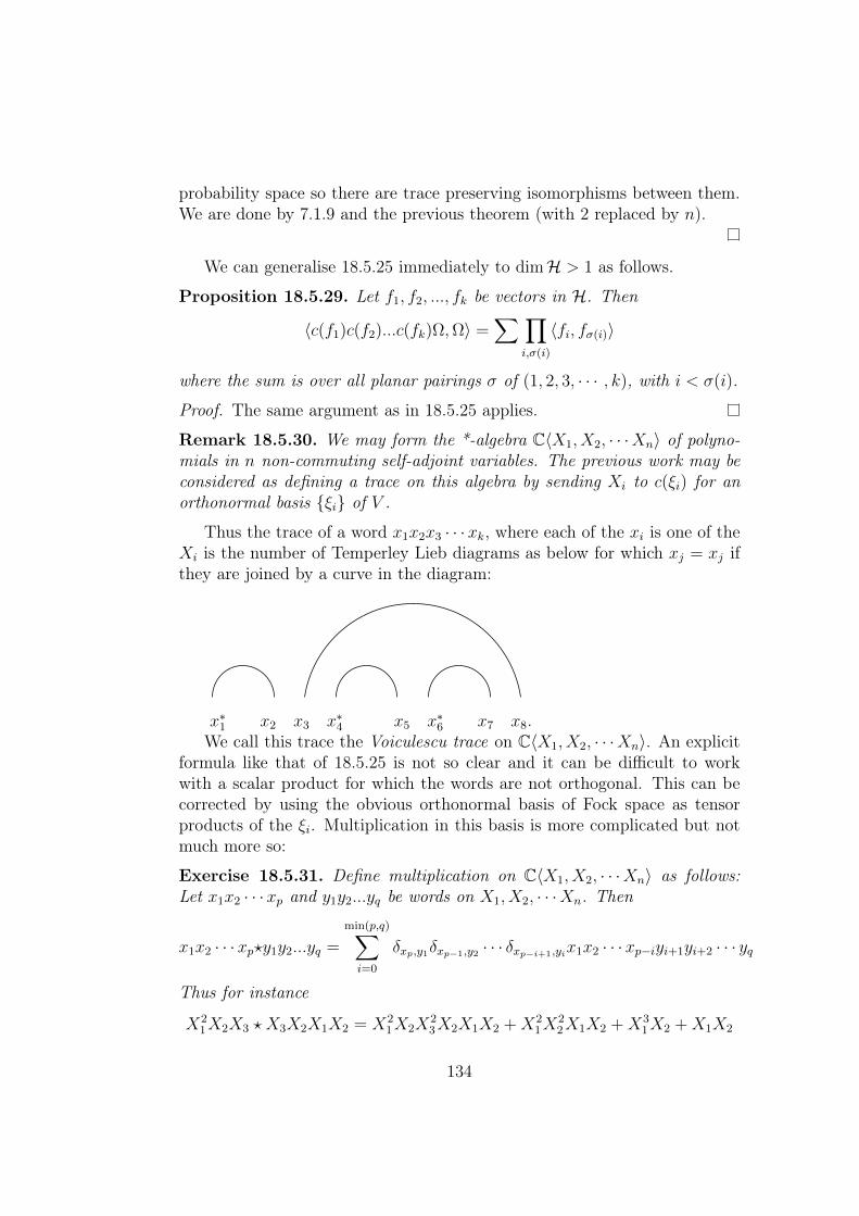
probability space so there are trace preserving isomorphisms between them.We are done by 7.1.9 and the previous theorem (with 2 replaced by n).

We can generalise 18.5.25 immediately to dimH > 1 as follows.

Proposition 18.5.29. Let f1, f2, ..., fk be vectors in H. Then

〈c(f1)c(f2)...c(fk)Ω,Ω〉 =∑∏

i,σ(i)

〈fi, fσ(i)〉

where the sum is over all planar pairings σ of (1, 2, 3, · · · , k), with i < σ(i).

Proof. The same argument as in 18.5.25 applies.

Remark 18.5.30. We may form the *-algebra C〈X1, X2, · · ·Xn〉 of polyno-mials in n non-commuting self-adjoint variables. The previous work may beconsidered as defining a trace on this algebra by sending Xi to c(ξi) for anorthonormal basis ξi of V .

Thus the trace of a word x1x2x3 · · ·xk, where each of the xi is one of theXi is the number of Temperley Lieb diagrams as below for which xj = xj ifthey are joined by a curve in the diagram:

x∗1 x2 x3 x∗4 x5 x∗6 x7 x8.We call this trace the Voiculescu trace on C〈X1, X2, · · ·Xn〉. An explicit

formula like that of 18.5.25 is not so clear and it can be difficult to workwith a scalar product for which the words are not orthogonal. This can becorrected by using the obvious orthonormal basis of Fock space as tensorproducts of the ξi. Multiplication in this basis is more complicated but notmuch more so:

Exercise 18.5.31. Define multiplication on C〈X1, X2, · · ·Xn〉 as follows:Let x1x2 · · ·xp and y1y2...yq be words on X1, X2, · · ·Xn. Then

x1x2 · · ·xp?y1y2...yq =

min(p,q)∑i=0

δxp,y1δxp−1,y2 · · · δxp−i+1,yix1x2 · · ·xp−iyi+1yi+2 · · · yq

Thus for instance

X21X2X3 ? X3X2X1X2 = X2

1X2X23X2X1X2 +X2

1X22X1X2 +X3

1X2 +X1X2

134

We would like to show how the Voiculescu trace arises in the study of largerandom matrices. For this we will use Wick’s theorem concerning jointlyGaussian random variables. A complex (centred) Gaussian random vari-able is a sum A+ iB of two independent identically distributed real centredGaussian random variables. The variance of A + iB is

√E(A2) + E(B2),

and E((A + iB)2) = 0. Suppose Z1, Z2 · · ·Zn are complex centred jointlyGaussian random variables with E(ZiZj) = aij.

Theorem 18.5.32.

E(Z1Z2 · · ·Zn) =∑σ

∏i<σ(i)

aiσ(i)

where the sum is over all pairings σ of 1, 2, · · ·n.

Now let X = Xij be a self-adjoint N × N random matrix. This meansthat the Xij are jointly Gaussian complex random variables with

Xij = Xji for i 6= j and Xiiis real,

and all other matrix entries are independent. Suppose E(|Xij|2) = d.Wewant to consider E(Trace(Xk)). Writing this out in full we get

∑i1,i2,···ik

E(Xi1i2Xi2i3Xi3i4 · · ·Xiki1).

The individual terms in this sum can each be expanded using Wick’sformula. In the figure below we have represented a typical term in the ex-pansion, each black dot being an occurrence of X and the pairing is indicatedby curves outside the circle. We have used a circle rather than a straight linesegment to emphasize the cyclic aspect of the trace.

135

5

i ii

i

i

ii

ii

ii

iiiii

i

i

i1 2

3

i3

4

5

6

6

7

7

8

8

1 2

4

Because of the independence of the Gaussians we will only get a non-zerocondition when k is even and the indices at one end of the pairing are thesame as at the other end, but in the opposite order. In order to get a non-zerocontribution, In the figure above this forces i1 = i4, i4 = i6, i6 = i3, i3 = i2and i7 = i1. So in fact there are only 3 freely varying indices, i1, i5 andi8 each of which gives a contribution to the total sum of d3. We representeach such contribution below where we have thickened the curves definingthe pairing into (flat) ribbons. Observe that the indices i1, i5 and i8 extendto the boundary components of the surface obtained by gluing the ribbonsto a central disc. There are N3 ways to assign the indices and once assigned,each term contributes dk/2. So the total contribution of all terms with thegiven pairing is N3dk/2.

136

5

i ii

i

i

ii

ii

ii

iiiii

i

i

i1 1

1

i1

1

5

1

1

1

1

8

8

1 1

1

Now consider a general pairing and proceed in the same way. If we glue in(abstract) discs along the boundary components we get an orientable surfacewhose Euler characteristic is “V-E+F" which in general will be 1− k/2 + Fwhere F is the number of discs glued in, i.e. the number of freely varyingindices for the given pairing. If g is the genus of the surface, we have 2−2g =F + 1− k/2 which gives

F = k/2 + 1− 2g.

So the total contribution of all terms with the given pairing is NFdk/2. We seethat if d = 1√

Nthen this contribution will be N1−2g so that 1

NE(Trace(Xk))

will tend, as N →∞, to the number of pairings with g = 0. But if the pairingis planar, obviously g = 0 and if g = 0 we know from the classification ofsurfaces that we get a 2-sphere, from which it is clear that the partition isplanar! Hence we have shown:

limN→∞

1

NE(Trace(Xk)) =

0 if k is odd

1m+1

(2mm

)if k = 2m

The above argument works equally well with n random N ×N matricesX1, X2, · · ·Xn each of which has entries with covariance as above and forwhich entries in different random matrices are independent. We see we haveproved the following:

137

Theorem 18.5.33. If w is a word on the random matrices X1, X2, · · ·Xn

as above then limN→∞1NE(Trace(w)) exists and is equal to the Voiculescu

trace of the same word viewed as an element of C〈X1, X2, · · ·Xn〉.

This result, together with 18.5.28 gave Voiculescu a remarkable new in-sight into the vN(Fn) and he was able to prove some spectacular isomor-phisms between them -[].

138

Chapter 19

Subfactors

19.1 Warmup. Finite Groups.

Let G be a finite group with an outer action α on the type II1 factor M . LetN = MG be the fixed point algebra. We continue the notational conventionsfrom chapter 11 on the crossed product.

A covariant representation of (M,α) is an action of M on some Hilbertspace H together with a unitary representation vg on H with vgxv∗g = αg(x)for g ∈ G and x ∈M .

Proposition 19.1.1. For finite groups the crossed product is universal forcovariant unitary representations. In fact any covariant representation of(M,α) extends to an isomorphism from M oG onto M, vg′′ by sendingug to vg.

Proof. Define π : M o G → M, vg′′ by π(∑

g agug) =∑

g agvg. π isobviously ultraweakly continuous so its image is a von Neumann algebra.But that image contains M and the vg. And a type II1 factor is simple.

A canonical way to obtain a covariant representation is to extend theaction of G on M to L2(M). We call these unitaries wg. We see that, forfinite groups only, another model for the crossed product is the von Neumannalgebra on L(M) generated by M and the wg.

Exercise 19.1.2. dimM M oG = |G|.

Proposition 19.1.3. The extension to L2(M) of the conditional expectationEN : M → N is eN = 1

|G|∑

g wg.

Proof. Obvious.

139

Theorem 19.1.4.

JN ′J = M ∪ wg′′ = M ∪ eN′′

Proof. Clearly J commutes with the wg and eN so the assertion is the sameas N ′ = M ′∪wg′′ = M ′∪eN′′. BothM ′ and the wg’s are in N ′ so itsuffices to prove that N ′ ⊆ M ′ ∪ eN′′ or equivalently M ′ ∪ eN′ ⊆ Nwhich follows from the assertion:

x ∈M and [x, eN ] = 0 =⇒ x ∈ N.

For this just evaluate xeN and eNx on the identity inside L2(M).

Remark 19.1.5. There is actually quite a bit of content here. How youwould write an individual wg for instance as an element of M ∪ eN′′?

Corollary 19.1.6. If G is a finite group acting by outer automorphisms on atype II1 factorM thenMG is a subfactor with trivial centraliser, dimMG(L2(M)) =|G| and (MG)′ ∩M oG = CG.

Proof. N is the commutant of a type II1 factor inside a type II1 factor, hencea type II1 factor. And N ′ ∩M = (M ′)′ ∩ M ′ ∪ vg′′ which is the scalarsby 19.1.1 and 11.2.5. For the dimension calculation note that by 11.2.5 weobtain M ⊆ M o G from any covariant representation. In particular wecan start with the crossed product on its own L2 space and reduce by aprojection of trace |G|−1 in its commutant. Thus by the formulae governingthe behaviour of dimM , dimM,wg′′ L

2(M) = |G|−1 and the result followsfrom 19.1.4. The last assertion is a trivial caclulation.

Exercise 19.1.7. If α is an outer action of the finite group G on the typeII1 factor M and ξ : G→ T is a one dimensional character, show there is aunitary u ∈M with

αg(u) = ξ(g)u ∀g ∈ G.Hint: try a 2x2 matrix argument, changing the action α⊗1 by Advg, vg beingthe unitary

(1 00 ξ(g)

).

The group G of all 1-dimensional characters ξ : G → T acts on M o Gvia the formula

αξ(∑g

agug) =∑g

ξ(g)agug

This is called the dual action.

140

Exercise 19.1.8. Show that the dual action (even for infinite groups G) isouter.

If G is abelian one may form the crossed product

(M oα G) oα G

Exercise 19.1.9. Show that if G is finite, the second dual action of G on(M oα G) oα G is conjugate to the "stabilised" action

α⊗ Ad`gon M ⊗ B(L2(G)) (where `g is the left regular representation).

The result of the previous exercise remains true for locally compact abeliangroups and motivates an alternative definition of the crossed product as thefixed points for the stabilised action.

19.2 Index.Inspired by the above and 10.2.2 we make the following:

Definition 19.2.1. If N ⊆M are II1 factors, the index [M : N ] of N in Mis the real number dimN L

2(M).

Exercise 19.2.2. Show that [M : N ] = 1 implies N = M .

Proposition 19.2.3. (i) If M acts on H so that dimN H <∞ then

[M : N ] =dimN HdimM H

.

(ii) If [M : N ] < ∞ and p is a projection in N ′ ∩M then set [M : N ]p =[pMp : pN ], then

[M : N ]p = trN ′(p)trM(p)[M : N ].

(for any action of M on H for which N ′is a type II1 factor.) (iii) If p isa partition of unity in N ′ ∩M then

[M : N ] =∑p

[M : N ]ptr(p)

.

(iv) If N ⊆ P ⊆M are type II1 factors then

[M : N ] = [M : P ][P : Q].

(v) If M acts on H such that dimN H <∞ then

[M : N ] = [N ′ : M ′]

141

Proof. (i) Certainly M ′ (on H) is a type II1 factor since N ′ is and taking thedirect sum of finitely many copies of H will not change the ratio dimN H

dimM H. So

we may assume dimM H ≥ 1 which means there is a projection p in M ′ withpH ∼= L2(M) as an M module. But the trace of this p in N ′ is the same asthe trace in M ′ by uniqueness of the trace. Hence by the properties of thecoupling constant, dimN H

dimM Hdoes not change under reduction by this p.

(ii) This follows immediately from (i) and properties of the coupling constant.(iii) Just sum [M :N ]p

trM (p)over p.

(iv) The only case of interest is when [M : N ] <∞. Then the result followsimmediately from (i).(v) Immediate from (i).

Corollary 19.2.4. If N ′ ∩M 6= Cid then [M : N ] ≥ 4.

Definition 19.2.5. We call a subfactor irreducible if N ′ ∩M = Cid.

Definition 19.2.6. A subfactor N ⊆M is called locally trivialif [M : N ]p = 1 for any minimal projection in N ′ ∩M .

Exercise 19.2.7. Show that dim(N ′ ∩M) ≤ [M : N ].

Here is a list of what might be called the "classical" subfactors- oneswhose existence owes nothing to the dedicated development of subfactor the-ory.

Example 19.2.8. The trivial subfactors.If M is a type II1 factor, so is M ⊗Mk(C) for any integer k > 0. We can

embed M in M ⊗Mk(C) by x 7→ x ⊗ 1. It is clear that L2(M ⊗Mk(C)) isthe direct sum of k2 copies of L2(M) so [M ⊗Mk(C) : M ] = k2.

Example 19.2.9. Continuously varying index.Choose a projection of trace d in the hyperfinite type II1 factor R. ThenpRp and (1 − p)R(1 − p) are isomorphic by hyperfiniteness so choose a vonNeumann algebra isomorphism θ : pRp→ (1− p)R(1− p). Let M be R andN be the subalgebra x + θ(x)|x ∈ pRp. It is clear that pMp = Np and(1− p)M(1− p) so by lemma 19.2.3,

[M : N ] =1

d+

1

1− d.

As d varies between 0 and 1, this index takes all real values ≥ 4.

Observe though that N ′∩M contains p so the subfactor is reducible. Theset of index values for irreducible subfactors of R is not understood thoughfor other type II1 factors it may be the interval [4,∞]

142

Example 19.2.10. Group-subgroup subfactors.If G is a discrete group acting by outer automorphisms on the type II1 factorM , and H is a subgroup of G, it is clear that M ⊗H is a subfactor of M ⊗Gof index [G : H].

If G is finite we may consider MG ⊆ MH which also has index [G : H]by 19.1.2 and 19.2.3

Example 19.2.11. Making the trivial non-trivial.

Definition 19.2.12. An action of a compact group on a factor M is calledminimal if (MG)′ ∩M = Cid.

If G has a minimal action α on M and ρ is an irreducible unitary repre-sentation of G on Ck we may take the action α⊗ Adρ on M ⊗Mk(C). Onethen defines the "Wassermann subfactor"

(M ⊗ 1)G ⊆ (M ⊗Mk(C))G.

The point is that the commutant of (M ⊗ 1)G in M ⊗Mk(C) is already justMk(C) by minimality of the action. So the fixed points are indeed factorsand the Wassermann subfactor is irreducible.

Already for finite groups this provides lots of examples. If G is infinitethere is a simple way to construct minimal actions. Just take a finite dimen-sional unitary representation ρ and consider ⊗∞1 Adρ on R. The group S∞ iscontained in the fixed points via its (inner) action permuting the tensor prod-uct factors. Moreover if we choose an orthonormal basis xi|i = 1, 2, ...k2 forMk(C) with x1 = 1, an orthonormal basis of R is formed by tensors ⊗∞j=1xi(j)indexed by functions i : N → 1, 2, · · · , k2 with i(j) = 1 for sufficientlylarge j. The action of S∞ on this basis has only one finite orbit-that of theidentity. So the only fixed points on in L2(R) are the scalar multiplies of theidentity.

Example 19.2.13. Finitely generated discrete groups.This example shows that finite index subfactors can be infinite objects indisguise. Let Γ = 〈γ1, γ2 · · · γk〉 be a finitely generated discrete group. Wehave seen that Γ can act in lots of ways, in particular outer, on type II1factors. Choose any action on M and for each x in M define the matrixd(x) = xi,j over M by

xi,j =

0 if i 6= j

γi(x) if i = j

143

Then consider the subfactor

D(M) = d(x)|x ∈M ⊆M ⊗Mk(C).

This subfactor is locally trivial so its index is k2 and one may think of it asa "twisted" version of the trivial subfactor of index k2.

Exercise 19.2.14. Show that dim(D(M)′ ∩M ⊗Mk(C)) = k iff γ−1i γj is

outer whenever i 6= j.

In fact one may easily extract the image of Γ modulo inner automorphismsfrom the subfactor D(M).

We now want to consider an entirely arbitrary subfactor. For this the fol-lowing "basic construction" is important. We have already seen its usefulnessfor finite group actions.

Proposition 19.2.15. Let N ⊆ M be a type II1 factors acting on L2(M)and let eN be the extension to L2 of the trace-preserving conditional ENexpectation onto N . Then

JN ′J = (JNJ)′ = M, eN”.

Proof. Already done in 19.1.4.

Definition 19.2.16. The von Neumann algebra 〈M, eN〉 = M, eN” of theprevious result is said to be the "basic construction" for N ⊆M .

Here are the most important facts about the basic construction. It willbe convenient from now on to use τ for [M : N ]−1. Since 〈M, eN〉 is a typeII1 factor its trace is unique and its restriction to M is the trace of M . Sowe just use tr for it.

Proposition 19.2.17.(i) For x ∈M, [x, eN ] = 0 iff x ∈ N .(ii) eNxeN = EN(x)eN for x ∈M .(iii) [M : N ] <∞ iff 〈M, eN〉 is a type II1 factor, in which case

[〈M, eN〉 : M ] = [M : N ].

(iv) M +MeNM is a weakly dense *-subalgebra of 〈M, eN〉.(v) eN〈M, eN〉eN = NeN(vi) tr(eN) = [M : N ]−1

(vii) For x ∈M , tr(eNx) = τtr(x)

144

Proof. (i) was done in 19.1.4.(ii) is a consequence of the bimodule property of EN on the dense subspaceM of L2(M).(iii) is immediate from proposition 19.2.15.(iv) Closure ofM+MeNM under multiplication follows from (ii). It containsM and eN hence is dense.(v) Follows immediately from (ii) and (iv).(vi) Follows from (v) and the behaviour of the coupling constant under re-duction by projections-note that eN(L2(M)) = L2(N).(vii) tr(xeN) = tr(eNxeN) = tr(eNxeN) = tr(EN(x)eN) = τ(EN(x) wherewe deduce the last equality from uniqueness of the trace on the type II1 factorN . Since the conditional expectation preserves the trace, we are done.

From now on we will use τ for [M : N ]−1.

Corollary 19.2.18. There is no subfactor N ⊆M with 1 < [M : N ] < 2.

Proof. By the uniqueness of the trace we see that trN ′(eN) = τ . Thus trN ′(1−eN) = 1− τ . Hence [(1− eN)〈M, eN〉(1− eN) : N(1− eN)] = (1− τ)2(1/τ)2

which is less than 1 if 1/2 < τ < 1.

If we suppose [M : N ] < ∞ we see we may do the basic constructionfor M ⊆ 〈M, eN〉. In the type II1 factor 〈〈M, eN〉, eM〉 we have the twoprojections eM and eN .

Proposition 19.2.19.

eMeNeM = τeM and eNeMeN = τeN

.

Proof. For the first relation we must show that EM(eN) = τid. But this isjust another way of saying (vii) of 19.2.17.To prove the second relation, by (iv) of 19.2.17 it suffices to apply each sideto elements of the form x + yeNz ∈ L2(〈M, eN〉) for x, y, z ∈ M . To do thisnote that eN acts by left multiplication.

Corollary 19.2.20. If [M : N ] 6= 1 then

eM ∨ eN =1

1− τ(eN + eM − eMeN − eNeM)

Proof. The relations show that eN and eM generate a 4-dimensional non-commutative algebra. By our analysis of two projections its identity mustbe a multiple of (eM − eN)2. The normalisation constant can be obtained byevaluating the trace.

145

Note that the special case eN ∨ eM = 1 (which is equivalent to τ = 1/2or index 2) means that eN and eM satisfy an algebraic relation.

Exercise 19.2.21. Use this relation to prove that, in index two, 〈〈M, eN〉, eM〉is the crossed product of 〈M, eN〉 by an outer action of Z/2Z. Use dualityto deduce Goldman’s theorem ([]): a subfactor of index 2 is the fixed pointalgebra for an outer Z/2Z action.

Let φ be the golden ratio 1+√

52

.

Corollary 19.2.22. There is no subfactor N ⊆M with 2 < [M : N ] < φ2.

Proof. We see that eN and eM are equivalent in the algebra they generateso their traces are equal wherever they are. Thus tr〈〈M,eN 〉,eM 〉(eN∨M) =trN ′(eN∨M) = 2τ and

[(1− eN ∨ eM)〈〈M, eN〉, eM〉(1− eN ∨ eM) : (1− eN ∨ eM)N ] = (1− 2τ)2τ−3

This is less than 1 if φ−2 < τ < 1/2.

If we did yet another basic construction in the same way and calculatedthe trace of the supremum of the three conditional expectations we wouldconclude that there is no subfactor with index between φ2 and 3. But it ishigh time to systematise the process.

19.3 The tower of type II1 factors and the ei’s.Definition 19.3.1. Let N ⊆ M be a subfactor of finite index τ−1. SetM0 = N,M1 = M and define inductively the tower of type II1 factors

Mi+1 = 〈Mi, eMi−1〉.

Set ei = eMi−1for i = 1, 2, 3, · · · .

Proposition 19.3.2. The ei’s enjoy the following properties.(i) e2

i = e∗i = ei(ii) eiej = ejei if |i− j| ≥ 2(iii) eiei±1ei = τei(iv) tr(wei+1) = τtr(w) for any word w on e1, e2, · · · ei.

Proof. These are all trivial consequences of the 19.2.17 and 19.2.20. Notethat the trace in (iv) is unambiguous by uniqueness of the trace on a typeII1 factor.

146

The relations of proposition 19.3.2 were discovered, albeit in a slightlydisguised form, in statistical mechanics in [], and were presented in almostthe above form in [] although property (iv) does not appear. With a beautifulinsight they were given a diagrammatic form in []. They are now universallyknown, in whatever form, as the Temperley-Lieb relations or the Temperley-Lieb algebra. We present Kauffman’s diagrammatics in the appendix A.

There is a lot of interesting combinatorics going with the Temperley-Liebalgebra but we want to get directly to the results on index for subfactors.Here are some exercises to familiarise the reader with these relations.

Exercise 19.3.3. Any word w on e1, e2, · · · en which is reduced in the obvioussense with respect to the relations 19.3.2 contains en (and e1) at most once.

Exercise 19.3.4. The dimension of the algebra generated by 1 and e1, e2, · · · enis at most

1

n+ 2

(2n+ 2

n+ 1

)(This exercise is the first hint that there might be some connection be-

tween subfactors and random matrices-see 18.5.25.)

19.4 Index restrictionsIt is clear from the restrictions we have obtained so far that we should beinterested in the trace of the sup of the first n ei’s.

Definition 19.4.1. Let Pn(τ) be the polynomials defined by P0 = 1, P1 = 1and

Pn+1 = Pn − τPn−1

Thus P2 = 1 − τ = tr(1 − e1), P3 = 1 − 2τ = tr(1 − e1 ∨ e2) andP4(τ) = 1− 3τ + τ 2.

Exercise 19.4.2. Define q by τ−1/2 = q+q−1. Show that Pn(τ) is essentially

the "quantum integer" [n+ 1]q =qn+1 − q−n−1

q − q−1, to be precise

Pn(τ) =[n+ 1]q([2]q)n

Definition 19.4.3. Put f0 = 1 and for each n = 1, 2, 3, · · · let

fn = 1− e1 ∨ e2 ∨ · · · ∨ en

.

147

Note that the fn are decreasing.

Theorem 19.4.4. If fn 6= 0 then

tr(fn+1) = Pn+2(τ)

Proof. Observe that the assertion is true for n = 0. Now suppose it is trueup to n. For convenience set sn = 1 − fn = e1 ∨ e2 ∨ e3 · · · ∨ en. We wantto calculate tr(sn ∨ en+1) and we know tr(sn) and tr(en). So it suffices tocalculate tr(sn ∧ en+1). To do this note that en+1snen+1 = EMn(sn)en+1 by19.2.17, and EMn(sn) is in the algebra generated by 1, e1, e2, · · · en−1 by19.3.3 and (iv) of 19.3.2. But by the bimodule property for a condionalexpectation eiEMn(sn) = EMn(sn)ei = ei for i ≤ n − 1. So snEMn(sn) isthe identity for the algebra generated by e1, e2, · · · en−1 and EMn(sn−1) =sn−1+(1−sn−1)EMn(sn). However 1−sn−1 is a minimal and central projectionin this algebra so

EMn(sn) = sn + λ(1− sn)

for some constant λ. Obviously 0 ≤ λ ≤ 1 because conditional expectationsdo not increase norms. But if λ were equal to 1, we would have EMn(sn) = 1which implies sn = 1, i.e. fn = 0 by faithfulness of the conditional expecta-tion. Thus λ < 1 and taking the limit as k →∞ of (en+1snen+1)k,

en+1 ∧ sn = en+1sn−1

Taking the trace we see that tr(en+1 ∧ sn) = τtr(sn−1).Finally tr(sn+1) = tr(sn)+τ−τtr(sn−1) and tr(fn+1) = tr(fn)−τtr(fn−1).

By induction and the definition of the Pn we are through.

The formula of the next theorem is due to Wenzl in [] which containscomplete information about families of projections on Hilbert space satisfying(i),(i) and (i)

Theorem 19.4.5. If fn 6= 0 then

fn+1 = fn −Pn(τ)

Pn+1(τ)fnen+1fn

Proof. It is easy to check for n = 1 and n = 2 for good measure.So suppose fn 6= 0. Then by the previous result Pn+1(τ) 6= 0 and we may

consider the element x = fn −Pn(τ)

Pn+1(τ)fnen+1fn. Obviously eix = 0 = xei

148

for i ≤ n and en+1x = en+1fn− Pn(τ)Pn+1(τ)

EMn(fn)en+1fn. By induction and thedefinition of Pn,

EMn(fn) =Pn+1(τ)

Pn(τ)fn−1

Since the fn are decreasing we get en+1x = 0 = xen+1 which means x is a(possibly zero) multiple of fn+1. But the trace of x is Pn+2(τ) so we are doneby the previous theorem.

Theorem 19.4.6. Let N ⊆M be type II1 factors. Then if [M : N ] < 4 it is4 cos2 π/n for some n = 3, 4, 5, . . . .

Proof. Observe that Pn(0) = 1 for all n. If we put q = eiθ in 19.4.2 we seethat τ−1 = 4 cos2 θ and

Pn−1(τ) =sinnθ

2n−1 sin θ(cos θ)n−1

This is zero for q a 2nth. root of unity (except q = 1) and the one withlargest cosine is θ = π/n. Thus the smallest real zero of Pn is 1

4 cos2 π/(n+1).

Moreover π/(n+1) < π/n < 2π/(n+1). So Pn+1(τ) < 0 between 14 cos2 π/(n+1)

and 14 cos2 π/n

while Pk(τ) > 0 for k ≤ n and τ in the same interval. Thusif τ is strictly between 1

4 cos2 π/(n+1)and 1

4 cos2 π/nwe conclude that fn > 0 and

tr(fn+1) < 0 which is impossible.

19.5 Finite dimensions

It is nice to have these restrictions on the values of the index but at thisstage the only values we know between 1 and 4 are 2 and 3. We will showthat all the values of theorem 19.4.6 actually occur. We will use a kindof "bootstrap" method. If the value of the index exists then there are ei’ssatsfying the relations of 19.3.2. But then we may consider the von Neumannalgebra in the towerMn generated by e1, e2, e3, · · · . We will show that thisis a factor. Moreover we will see that the subfactor generated by e2, e3, · · · will be seen to have index τ−1. But this presupposes the existence of thesubfactor! For τ < 1/4 we can get the ei’s from the tower obtained fromexample 19.2.9. For τ ≥ 1/4 we will be able to construct a tower comingfrom inclusions A ⊆ B of finite dimensional von Neumann algebras whichgets around the problem. For this we obviously need to know how the basicconstruction works in finite dimensions.

149

Recall from 4.4.3 that a unital inclusion A ⊆ B of finite dimensional vonNeumann algebras is given by a vector ~v whose entries are labelled by theminimal central projections of A and a matrix Λ = λp,q where q runs over theminimal central projections in A an p over the minimal central projections inB. Λ~v is then vector whose entries are the ranks of the simple components ofB. If e ≤ p is minimal in A and f ≤ q is minimal in B then ef is a projectionof rank λp,qin the factor qB.

Definition 19.5.1. We call ~v as above the dimension vector of a finite di-mensional von Neumann algebra and the matrix Λ the inclusion matrix. Wewill write ~vA and ΛB

A if we need to specify which algebras we are talking about.We will say the inclusion is connected if Z(A) ∩ Z(B) = Cid, which can berecognised by connectedness of the obvious bipartite graph associated to theinclusion matrix.

Thus in full:

ΛBA~vA = ~vB

This information is conveniently recorded graphically:

1

5 4

2 3

Here A = M2(C)⊕M3(C)⊕C so ~vA =(

231

)and B = M5(C)⊕M4(C) so

~vB = ( 54 ). There is no "multiplicity" so minimal projections in A are sums

of minimal projections in different simple components of B and the inclusionmatrix is ( 1 1 0

0 1 1 ).

Exercise 19.5.2. If A ⊆ B and B ⊆ C then ΛCA = ΛC

BΛBA.

This can be done by pure thought observing that ΛBA is just the matrix

of the inclusion map from K0(A) to K0(B).The basic construction can be performed without recourse to a trace

simply by defining it as the commutant on B of the right action of A whichallows us to identify its centre with that of A. But we are after the ei’s solets use (positive) traces.

Definition 19.5.3. If A is a finite dimensional von Neumann algebra withtrace tr define the trace vector ~tr to be the row vector whose entries are

150

indexed by the central projections of A and whose pth. entry is tr(e), e beinga minimal projection in A, e ≤ p.

Remark 19.5.4.(i)A trace is clearly normalised iff ~tr · ~vA = 1.(ii) If A ⊆ B are as above and Tr is a trace on B whose restriction to A istr then:

~TrΛ = ~tr

Given a (normalised) faithful trace Tr on B we may perform the basicconstruction 〈B, eA〉 exactly as for type II1 factors.

The centre of 〈B, eA〉 can be identified with that of A by x 7→ JxJ so theinclusion matrix for B ⊆ 〈B, eA〉 will have the same shape as the transposeof that of A ⊆ B.

Exercise 19.5.5. Show that

Λ〈B,eA〉B = (ΛB

A)t

Thus in the example above we would get the "Bratteli" diagram:

4

5 4

2 3 1

5 9

for the tower A ⊆ B ⊆ 〈B, eA〉.In the non-factor case there is no canonically defined trace on the basic

construction. For obvious reasons we would like to have such a trace TRwith the crucial property TR(eAx) = τTr(x) for x ∈ B.

Theorem 19.5.6. If A ⊆ B is a connected inclusion with matrix Λ, there isa unique normalised trace Tr on B which extends to a trace TR on 〈B, eA〉such that EB(eA) ∈ Cid. ~TRΛΛt = τ−1 ~TR for τ satisfying EB(eA) = τeA.

Proof. Observe that if f is a minimal projection in A then eAf is a minimalprojection in 〈B, eA〉 by (v) of 19.2.17. If p is a minimal central projectionin A with pf = f , we want to show that eAf is under JpJ . To do this it isenough to show that JpJeAf 6= 0. But applying it to the identity in B we getfp. So if Tr has an extension TR satisfying TR(eAx) = τTr(x) for x ∈ B,

151

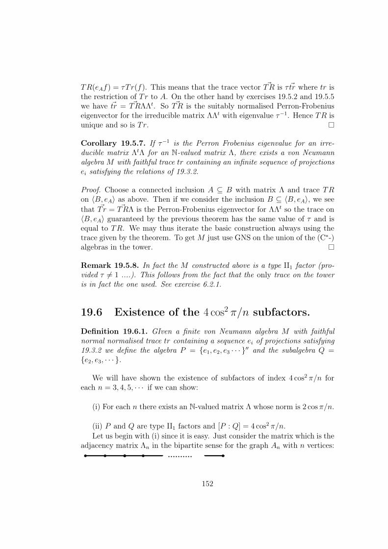
TR(eAf) = τTr(f). This means that the trace vector ~TR is τ ~tr where tr isthe restriction of Tr to A. On the other hand by exercises 19.5.2 and 19.5.5we have ~tr = ~TRΛΛt. So ~TR is the suitably normalised Perron-Frobeniuseigenvector for the irreducible matrix ΛΛt with eigenvalue τ−1. Hence TR isunique and so is Tr.

Corollary 19.5.7. If τ−1 is the Perron Frobenius eigenvalue for an irre-ducible matrix ΛtΛ for an N-valued matrix Λ, there exists a von Neumannalgebra M with faithful trace tr containing an infinite sequence of projectionsei satisfying the relations of 19.3.2.

Proof. Choose a connected inclusion A ⊆ B with matrix Λ and trace TRon 〈B, eA〉 as above. Then if we consider the inclusion B ⊆ 〈B, eA〉, we seethat ~Tr = ~TRΛ is the Perron-Frobenius eigenvector for ΛΛt so the trace on〈B, eA〉 guaranteed by the previous theorem has the same value of τ and isequal to TR. We may thus iterate the basic construction always using thetrace given by the theorem. To getM just use GNS on the union of the (C∗-)algebras in the tower.

Remark 19.5.8. In fact the M constructed above is a type II1 factor (pro-vided τ 6= 1 ....). This follows from the fact that the only trace on the toweris in fact the one used. See exercise 6.2.1.

19.6 Existence of the 4 cos2 π/n subfactors.

Definition 19.6.1. GIven a finite von Neumann algebra M with faithfulnormal normalised trace tr containing a sequence ei of projections satisfying19.3.2 we define the algebra P = e1, e2, e3 · · · ′′ and the subalgebra Q =e2, e3, · · · .

We will have shown the existence of subfactors of index 4 cos2 π/n foreach n = 3, 4, 5, · · · if we can show:

(i) For each n there exists an N-valued matrix Λ whose norm is 2 cosπ/n.

(ii) P and Q are type II1 factors and [P : Q] = 4 cos2 π/n.Let us begin with (i) since it is easy. Just consider the matrix which is the

adjacency matrix Λn in the bipartite sense for the graph An with n vertices:..........

152

Thus for n = 2m even, Λn is m×m and for n = 2m+ 1 it is m× (m+ 1).In both cases

λi,j =

1 if i = j or j + 1

0 otherwise

Exercise 19.6.2. Show that ||Λn|| = 2 cos π/(n+ 1).

Note that these are not the only choices for Λ. If Λ is the bipartite adja-cency matrix for a Coxeter-Dynkin graph of type A, D or E one has:

||Λ|| = 2 cos π/n where n =

n+ 1 for An2n− 2 for Dn

12 for E6

18 for E7

30 for E8

These are the only possibilities for ||Λ|| < 2 (see []).

Now let us show that P (and hence obviously Q) is a factor.We will need a simple lemma.

Lemma 19.6.3. With notation as in 19.6.1, any normal trace on P is de-termined by its restriction to all commutative subalgebras of the form AI =ei|i ∈ I′′ where I is a subset of N with the property that

i, j ∈ I =⇒ |i− j| ≥ 2

.

Proof. If φ is a normal trace on P it is determined by its value on wordson the ei’s. But it is a simple matter to deduce from exercise 19.3.3 thatany word can be reduced after cyclic permuations to a multiple of a word inwhich all the indices of ei’s differ by at least two.

Theorem 19.6.4. Let P , M and tr be as in definition 19.6.1. Then P is atype II1 factor (provided τ 6= 1).

Proof. By 19.6.3 it suffices to show that any normal normalised trace on Pis equal to tr. But let φ be such a trace. Let I be as in 19.6.3. Embed I intoan infinite set J with the same property. Let i < j be elements of J withnothing in between i and j in J . We claim the the normaliser of AJ containsa self-adjoint unitary u such that ueiu = ej and ueku = ek for k 6= i, j.For this just consider the algebra generated by 1, ei, ei+1, ei+2 · · · ej. The

153

projections ei and ej are equivalent in this finite dimensional von Neumannalgebra and it is a simple exercise to see that two equivalent projections in amatrix algebra are always conjugate under a self-adjoint unitary.

But AJ is the infinite tensor product of copies of C2 with product stategiven by tr(ei) = τ . And the normaliser contains the group S∞ acting bypermuting the tensor product components. So just as in 19.2.11, the action ofS∞ is ergodic and there is only one invariant probability measure absolutelycontinuous with respect to tr. Thus tr = φ on AJ and we are done.

The last detail is to show that Q ⊆ P has the right index.

Theorem 19.6.5. [P : Q] = τ−1.

Proof. Perform the basic construction 〈P, eQ〉. P is spanned by words of theform ae1b with a and b in Q. Let R = e3, e4, · · · ′′. Using 19.3.2 we havee1(ae1b) = ER(a)e1b and e1eQe1(ae1b) = τER(a)e1b. And easily eQe1eQ =τeQ. Thus eQ and e1 are equivalent in 〈P, eQ〉.

We conclude first that 〈P, eQ〉 is a type II1 factor since eQ is a finiteprojection ( eQ〈P, eQ〉eQ = QeQ), and a finite projection in a II∞ factorcannot be in a II1 subfactor. So tr(eQ) = τ−1 since tr(e1) = τ−1.

19.7 The structure of the algebras En = e1, e2, · · · en′′.We have that En is finite dimensional but we will see that its dimensiondepends on τ . Clearly En ⊆ En+1 so there is a Bratteli diagram to compute.

Theorem 19.7.1. "Generically", that is for 0 < τ ≤ 1/4, the Bratteli dia-gram for the tower En is below:

Where E0 = Cid and we have recorded the traces of minimal projectionsin each simple summand.

Proof. The calculation of E0 ⊆ E1 ⊆ E2 is trivial. So proceed inductively.Then En+1 is obtained from En by adding en+1 which satisfies

en+1xen+1 = EEn−1(x)en+1 for x ∈ En

154

Appendix A

Kauffman’s diagrammatics for theTemperley-LIeb algebra.

155

156

Appendix B

Proof of the KMS condition.

Theorem B.0.2. Let φ be a faithful normal state on a von Neumann algebraM . Then the modular group σφt is the unique one parameter automorphismgroup of M which satisfies the KMS condition for φ.

Proof. Perform the GNS construction with canonical cyclic and separatingvector Ω and modular operators S = J∆1/2. Recall that f(∆)Ω = Ω for anyfunction of ∆ with f(1) = 1. In particular φ(σφt (x) = 〈(∆itx∆−itΩ,Ω〉 so σφtpreserves φ.

Now let us check the rest of the KMS condition. We have

φ(σφt (x)y) = 〈∆−ityΩ, x∗Ω〉

and

φ(yσφt (x)) = 〈yσφt (x)Ω,Ω〉= 〈J∆1/2σφt (x∗)Ω, J∆1/2yΩ〉= 〈∆1/2yΩ,∆1/2∆itx∗Ω〉= 〈∆1/2−ityΩ,∆1/2x∗Ω〉

So let ξ = yΩ, η = x∗Ω and let pn be the spectral projection for ∆ forthe interval [1/n, n] so that pn tends strongly to 1 and ∆±1 are bounded onpnHφ. The functions

Fn(z) = 〈∆−izpnξ, η〉

are then entire and

|Fn(t)− φ(σφt (x)y)| = |〈∆−it(1− pn)ξ, η〉| ≤ ||(1− pn)ξ|| ||η|||Fn(t+ i)− φ(yσφt (x))| = |〈∆1/2−it(1− pn)ξ,∆1/2η〉| ≤ ||(1− pn)∆1/2ξ|| ||∆1/2η||.

157

Hence the Fn are bounded and continuous on the strip z : 0 < =mz < 1and converge uniformly on its boundary. By the Phragmen-Lindelof theoremwe are done.

Now let us prove uniqueness of the modular group with the KMS condi-tion.

Let αt be another continous one-parameter automorphism group satisfy-ing KMS for φ. The fact that αt preserves φ means we can define a stronglycontinous one-parameter unitary group t 7→ ut by utxΩ = αt(x)Ω. By Stone’stheorem it is of the form t 7→ Dit for some non-singular positive self-adjointoperator A. The goal is to prove that D = ∆. As a first step we construct adense set of analytic vectors in MΩ by Fourier transform. Let A be the setof all operators of the form ∫ ∞

−∞f(t)αt(x)dx

for all C∞ functions f of compact support on R. The integral convergesstrongly so

f(log(D))xΩ =

∫ ∞−∞

f(t)Dit(xΩ)dx

is in AΩ. Thus the spectral projections of D are in the strong closure of Aand AΩ is dense. Moreover z 7→ DzxΩ is analytic for x ∈ A since xΩ isin the spectral subspace of A for a bounded interval. Also AΩ is invariantunder Dz by the functional calculus. To compare with φ define, for x and yin A, the entire function

F1(z) = 〈D−izyΩ, x∗Ω〉.Let F be the function, analytic inside the strip and continuous and boundedon it, guaranteed for x and y by the KMS condition. Then if we define G(z)for −1 ≤ =mz ≤ 1 by

G(z) =

F (z)− F1(z) if =mz ≥ 0;

F (z)− F1(z) if =mz ≤ 0.

Since F and F1 agree on the real line G is analytic for −1 < =mz < 1, hencecheck typesetting

equal to 0, and since both F and F1 are continous on the strip, φ(yσt(x)) =F (t+ i) = F1(t+ i) = 〈D1−ityΩ, x∗Ω〉. In particular putting t = 0 we get

〈DyΩ, x∗Ω〉 = φ(yx)

= 〈xΩ, y∗Ω〉= 〈J∆1/2x∗Ω, J∆1/2yΩ〉= 〈∆1/2yΩ,∆1/2x∗Ω〉

158

So ∆1/2yΩ is in the domain of ∆1/2 and ∆yΩ = DyΩ.

Thus D and ∆ agree on AΩ. But multiplication by the function ez + 1 isa linear isomorphism of C∞c so by functional calculus (D+1)AΩ = AΩ whichis thus dense. Since D + 1 is invertible by spectral theory, any (ξ, (D + 1)ξ)in the graph of D+1 can be approximated by (AnΩ, (D+1)AnΩ). Thus D isessentially self-adjoint on AΩ, and both ∆ and D are self-adjoint extensionsof the restriction of D to this domain. Thus D = ∆.

159

160

Bibliography

[1] F.M. Goodman, P. de la Harpe, and V.F.R. Jones, Coxeter graphs andtowers of algebras, Springer-Verlag, 1989.

[2] M. Reed and B. Simon, Methods of Modern Mathematical Physics I:Functional Analysis, Academic Press, 1972.

[3] M. Takesaki, Theory of Operator Algebras II. EMS series on OperatorAlgebras, 2002.

[4] J.-B. Bost and A.Connes, Hecke algbebras, type III factors and phasetransitions with spontaneous symmetry breaking in number theory, Se-lecta Math. (New Series),1, (1995), 411-457.

161