Horizon-based curvatureattributes have been used inseismic data interpretationfor predicting fracturessince 1994 when Lisle dem-onstrated the correlation ofcurvature values to frac-tures measured on an out-crop. Different measures ofcurvature (such as Gaus-sian, strike, and dip) havebeen shown by differentworkers to be highly corre-lated with fractures, andmany more applications arealso possible. By definition,all such applications needthe interpretation of a seis-mic horizon, which may besimple if data quality isgood and the horizon ofinterest corresponds to aprominent impedance con-trast.

In contrast, horizonspicked on noisy seismicdata contaminated by back-scattered noise and/oracquisition footprint, orpicked through regionswhere no consistent im-pedance contrast exists, can lead to inferior curvature mea-sures. One partial solution to noisy picks is to run a spatialfilter over them, taking care to remove the noise yet retainthe geometric detail.

A significant advance in the area of curvature attributesis the volumetric estimation of curvature at different wave-lengths introduced by Al-Dossary and Marfurt (2006). Thisvolumetric estimation of curvature alleviates the need forpicking horizons for regions in which no continuous sur-face exists. This paper reports our investigations into bothhorizon-based and volumetric curvature attribute applica-tions.

A key point is that, even after careful spatial filtering,horizon-based curvature estimates may still suffer from arti-facts. Conversely, curvature attribute values extracted fromcurvature attribute volumes along the same horizons yielddisplays free of artifacts and make more geologic sense.

Attributes and structure-oriented filtering. The purpose offiltering along seismic events is to remove noise and enhancelateral continuity. This can be done by differentiatingbetween the dip/azimuth of the reflector and that of theunderlying noise. Once the dip/azimuth has been estimated,a filter can enhance signal along the reflector, much as inter-preters do with time/structure and amplitude extractionmaps using interpretation workstation software. The famil-iar filters are the mean, median, and trimmed mean. While

these do a good job enhancing the signal-to-noise ratio ofthe data, they smear faults.

Hoecker and Fehmers (2002) address this problem byusing an “anisotropic diffusion” smoothing algorithm. Theanisotropic part is so named because the smoothing takesplace parallel to the reflector, while no smoothing takesplace perpendicular to the reflector. Most important, no

Volumetric curvature attributes add value to 3D seismic data interpretationSATINDER CHOPRA, Arcis Corporation, Calgary, CanadaKURT J. MARFURT, University of Houston, USA

856 THE LEADING EDGE JULY 2007

Figure 1. Two segments of a seismic section (a) before and (b) after the application of structure-oriented pcfiltering from a 3D seismic volume from Alberta, Canada. Notice the cleaner background and focused ampli-tudes of the seismic reflections after pc filtering as well as the preserved fault edges.

The subject of this article is covered more extensivelyin SEG’s newest publication, Seismic Attributes forProspect Identification andReservoir Characterization, byChopra and Marfurt. This456-page book introducesthe physical basis, mathe-matical implementation,and geologic expression ofmodern volumetric attrib-utes including coherence,dip/azimuth, curvature,amplitude gradients, seis-mic textures, and spectraldecomposition. Availablenow at www.seg.org.

JULY 2007 THE LEADING EDGE 857

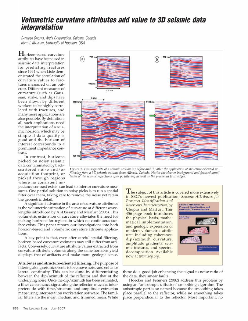
Figure 2. Time slices (at 1232 ms) from the seismic volume generated (a) before and (b) after structure-oriented pc filtering of data, shown inFigure 1, but from a different portion of the survey. Notice the reduced background noise and focused edges of the features on these time slicesafter pc filtering.

Figure 3. Segment of a seismic section from a 3D seismic volume from northeastern British Columbia, Canada (a) before and (b) after applicationof structure-oriented pc filtering. Notice the cleaner background and focused amplitudes of the seismic reflections after pc filtering as well as thepreserved fault edges. Time slices (at 1576 ms) from the seismic volume generated (c) before and (d) after pc filtering of the data shown in Figures3a and b. The position of the seismic lines shown above is indicated with dotted lines. Notice the reduced background noise and focused edges ofthe features on these time slices after pc filtering.

858 THE LEADING EDGE JULY 2007

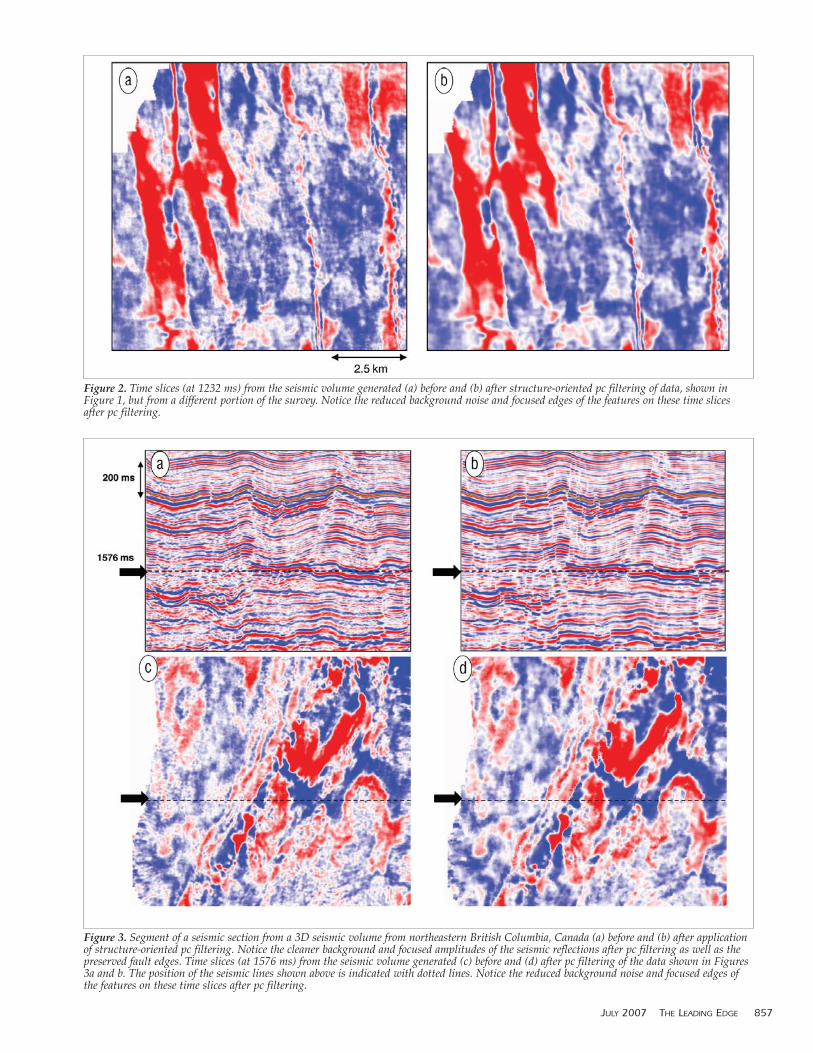
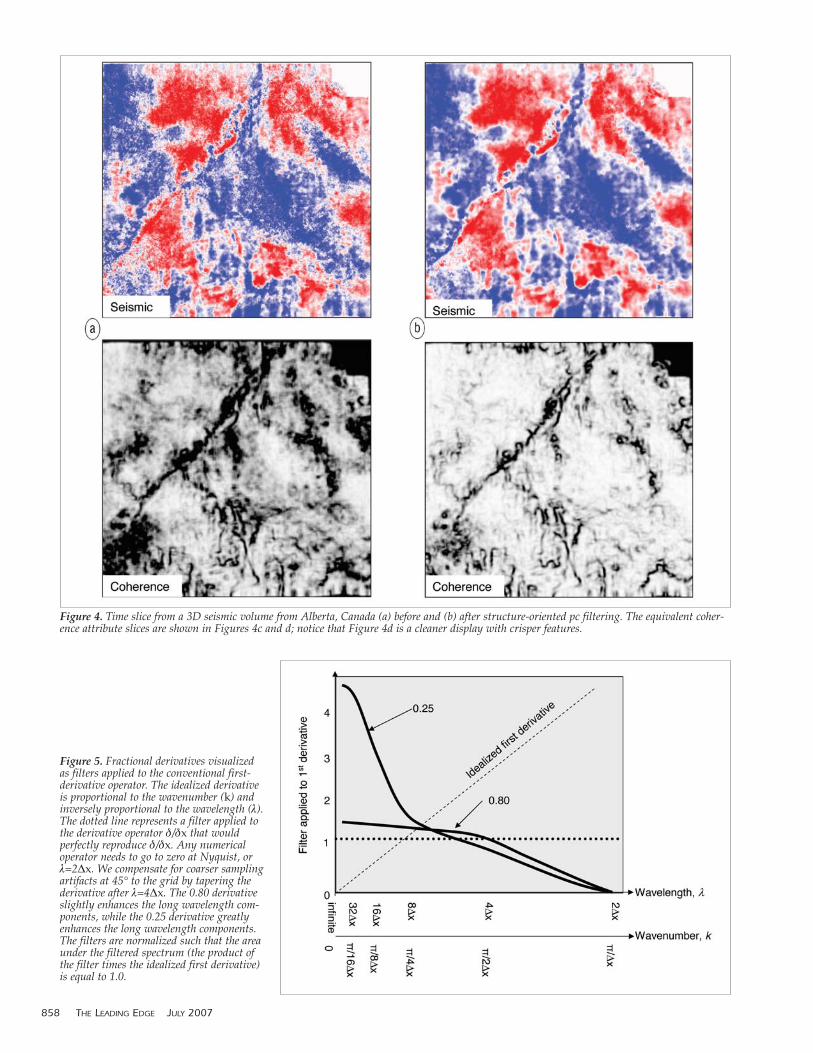
Figure 4. Time slice from a 3D seismic volume from Alberta, Canada (a) before and (b) after structure-oriented pc filtering. The equivalent coher-ence attribute slices are shown in Figures 4c and d; notice that Figure 4d is a cleaner display with crisper features.

Figure 5. Fractional derivatives visualizedas filters applied to the conventional first-derivative operator. The idealized derivativeis proportional to the wavenumber (k) andinversely proportional to the wavelength (λ).The dotted line represents a filter applied tothe derivative operator δ/δx that wouldperfectly reproduce δ/δx. Any numericaloperator needs to go to zero at Nyquist, orλ=2∆x. We compensate for coarser samplingartifacts at 45° to the grid by tapering thederivative after λ=4∆x. The 0.80 derivativeslightly enhances the long wavelength com-ponents, while the 0.25 derivative greatlyenhances the long wavelength components.The filters are normalized such that the areaunder the filtered spectrum (the product ofthe filter times the idealized first derivative)is equal to 1.0.

smoothing takes place if a discontinuity is detected, therebypreserving the appearance of major faults and stratigraphicedges. Luo et al.’s (2002) edge-preserved filtering proposeda competing method that uses a multiwindow (Kuwahara)filter to address the same problem. Both approaches use amean or median filter applied to data values that fall withina spatial analysis window with a thickness of one sample.

Marfurt (2006) describes a multiwindow (Kuwahara)principal component filter that uses a vertical window ofdata samples to compute the waveform that best representsthe seismic data in the spatial analysis window. Seismicprocessors may be more familiar with the principal com-ponent filter as the equivalent Kohonen-Loeve (or simplyKL) filter. In this paper, we use 99 nine-trace, ±10-ms (11-sample) analysis windows parallel to the dip/azimuth thatcontains the analysis point of interest. We then apply ourprincipal component (pc) filter to the analysis point usingthe window that contains the most coherent data. Becauseit uses (for our examples 11 times) more data, the pc filterin general produces significantly better results than the cor-responding mean filter. We advise the hopeful reader thatthere is no such thing as a “silver bullet” in seismic data

processing. If the data are contaminated by high-amplitudespikes, then a median, alpha-trim mean, or other nonlinearfilter will provide superior results. Likewise the pc filter willpreserve amplitude variations in coherent signal that mayexacerbate acquisition geometry, whereas a mean filter willsmooth them out.

Seismic data that have been pc filtered will in generalhave a higher signal-to-noise ratio, exhibit sharper discon-tinuities, and provide enhanced images of faults, fracturesand stratigraphic features such as channels. Autotrackerstend to work much better on filtered data, providing con-tinuous surfaces that stop at discontinuities. Attributesextracted from these data often yield more meaningful dis-plays than those from unfiltered data; however, not all fea-tures of geologic interests appear as edges. Structure-oriented filtering will smooth out and therefore diminishthe easily recognized “chaotic” textures associated withkarst, mass-transport complexes, and hydrothermally altereddolomite.

Figure 1 shows the result of pc filtering on a 3D seismicdata set from Alberta. Notice not only the overall cleanerlook of the section after pc filtering, but also the sharpen-

860 THE LEADING EDGE JULY 2007

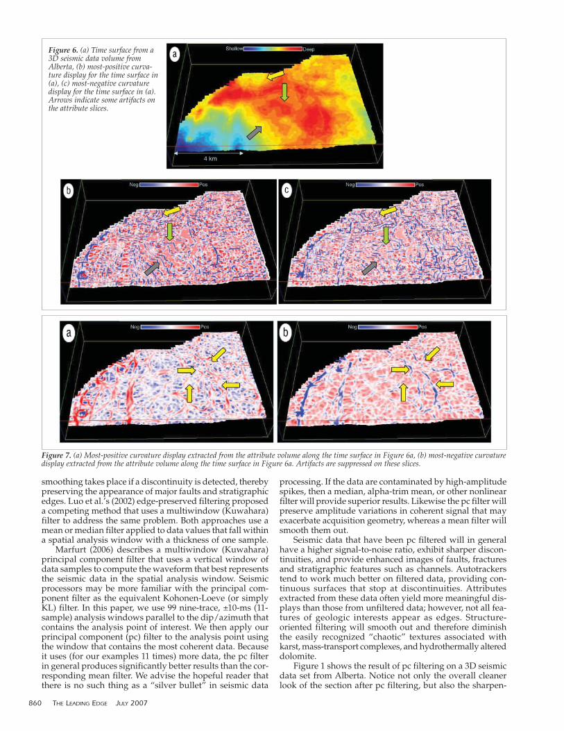
Figure 6. (a) Time surface from a3D seismic data volume fromAlberta, (b) most-positive curva-ture display for the time surface in(a), (c) most-negative curvaturedisplay for the time surface in (a).Arrows indicate some artifacts onthe attribute slices.

Figure 7. (a) Most-positive curvature display extracted from the attribute volume along the time surface in Figure 6a, (b) most-negative curvaturedisplay extracted from the attribute volume along the time surface in Figure 6a. Artifacts are suppressed on these slices.

ing of the vertical faults. Figure 2, from a different part ofthe same survey, compares time slices before and after pcfiltering; improved event focusing and reduced backgroundnoise levels after structure-oriented pc filtering are clearlyevident. Figure 3 shows a similar comparison of an inlineand a time slice before and after pc filtering.

Attributes computed from pc-filtered seismic data vol-umes. Attributes computed from seismic data having a goodsignal-to-noise ratio are bound to yield significantly moremeaningful information. Figures 4a and b show seismic andcoherence time slices before and after pc filtering. Not only

does the time slice in Figure 4b have better event definitionand lower noise level, but the coherence derived from thisdata set shows sharper lineaments and less incoherent noise.

Geologic structures often exhibit curvature of differentwavelengths, and curvature images having different wave-lengths provide different perspectives of the same geology.Tight (short-wavelength) curvature often delineates detailswithin intense, highly localized fracture systems. Broad(long-wavelength) curvature often enhances subtle flexures(on the scale of 100–200 traces, that are difficult to see in con-ventional seismic, but are often correlative to fracture zonesthat are below seismic resolution) and collapse features and

JULY 2007 THE LEADING EDGE 861

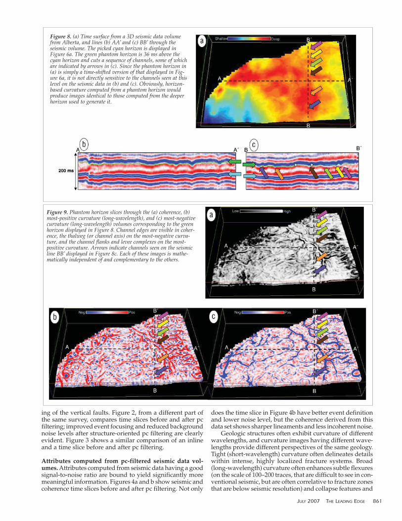
Figure 8. (a) Time surface from a 3D seismic data volumefrom Alberta, and lines (b) AA’ and (c) BB’ through theseismic volume. The picked cyan horizon is displayed inFigure 6a. The green phantom horizon is 36 ms above thecyan horizon and cuts a sequence of channels, some of whichare indicated by arrows in (c). Since the phantom horizon in(a) is simply a time-shifted version of that displayed in Fig-ure 6a, it is not directly sensitive to the channels seen at thislevel on the seismic data in (b) and (c). Obviously, horizon-based curvature computed from a phantom horizon wouldproduce images identical to those computed from the deeperhorizon used to generate it.

Figure 9. Phantom horizon slices through the (a) coherence, (b)most-positive curvature (long-wavelength), and (c) most-negativecurvature (long-wavelength) volumes corresponding to the greenhorizon displayed in Figure 8. Channel edges are visible in coher-ence, the thalweg (or channel axis) on the most-negative curva-ture, and the channel flanks and levee complexes on the most-positive curvature. Arrows indicate channels seen on the seismicline BB’ displayed in Figure 8c. Each of these images is mathe-matically independent of and complementary to the others.

diagenetic alterations that result in broader depressions. Al-Dossary and Marfurt introduced a “fractional deriva-

tive” approach for volume computation of multispectral esti-mates of curvature. They define the fractional derivative as

where the operator F denotes the Fourier transform, u is aninline or crossline component of reflector dip, and α is a frac-tional real number that typically ranges between 1 (givingthe first derivative) and 0 (giving the Hilbert transform) ofthe dip. The nomenclature fractional derivative was bor-rowed from Cooper and Cowans (2003); however, an astutemathematician will note that the i is not in the parentheses.

In this manner we can interpret the preceding equation assimply a low-pass filter of the form kx

(α-1) applied to a con-ventional first derivative. Figure 5 shows filters for valuesα=0.80 and α=0.25. Given the spectral response, particularlywhen multiplied by the spectral response of the derivativeoperator, we will call the resulting images “short-wave-length” and “long-wavelength” curvature in the figures thatfollow.

The space domain operators corresponding to differentvalues of α mentioned above are convolved with the pre-viously computed dip components estimated at every sam-ple and trace within the seismic volume. In addition, thedirectional derivative is applied to a circular rather than lin-ear window of traces, thereby avoiding a computational

862 THE LEADING EDGE JULY 2007

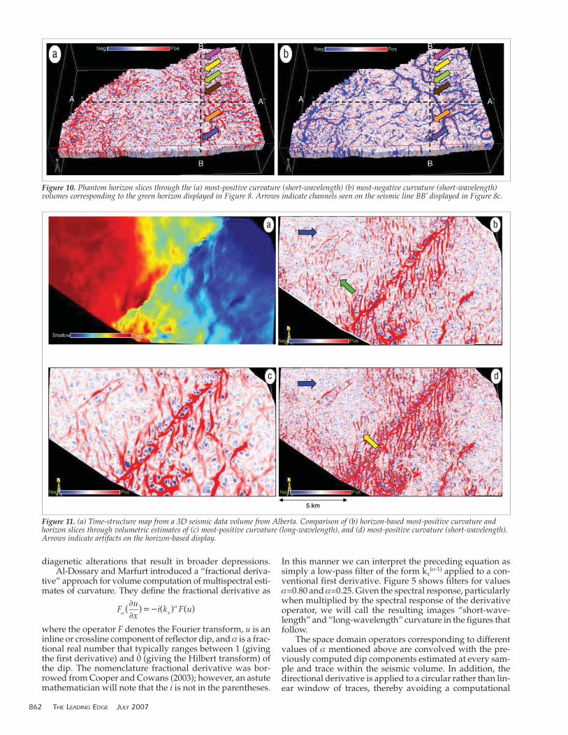
Figure 11. (a) Time-structure map from a 3D seismic data volume from Alberta. Comparison of (b) horizon-based most-positive curvature andhorizon slices through volumetric estimates of (c) most-positive curvature (long-wavelength), and (d) most-positive curvature (short-wavelength).Arrows indicate artifacts on the horizon-based display.

Figure 10. Phantom horizon slices through the (a) most-positive curvature (short-wavelength) (b) most-negative curvature (short-wavelength)volumes corresponding to the green horizon displayed in Figure 8. Arrows indicate channels seen on the seismic line BB’ displayed in Figure 8c.

bias associated with the acquisition axes. Lower values ofα decrease the contribution of the high frequencies, therebyshifting the bandwidth toward longer wavelength.

Curvature images of differential compaction over chan-nels. Figure 6a shows a time-structure map interpreted froma 3D seismic survey acquired in Alberta, Canada. This hori-zon was the nearest continuous event below a slightly shal-lower channel system of interest. We manually picked agrid of control lines, autotracked the horizon, and thenapplied a 3 � 3 mean filter to remove short wavelength jit-ter from the interpreted picks. Next, we computed the most-

positive and most-negative curvature directly from the auto-tracked and filtered horizon to generate the horizon-basedcurvature images in Figures 6a–c. Notice that both displaysare contaminated by a time contour overprint, as indicatedby the yellow, green and gray arrows. Such overprints areartifacts that do not make any geologic sense. We do not seeany clear evidence of the channel system overlying thishorizon.

Next, we computed volumetric estimates of most-posi-tive and most-negative curvature corresponding to everysample in the seismic volume and displayed horizon slicesthrough both attribute volumes (Figure 7). This is a short-

864 THE LEADING EDGE JULY 2007

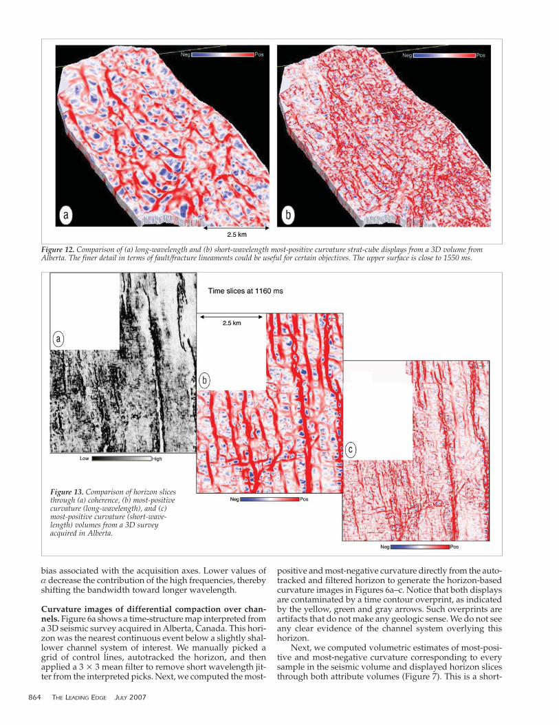
Figure 12. Comparison of (a) long-wavelength and (b) short-wavelength most-positive curvature strat-cube displays from a 3D volume fromAlberta. The finer detail in terms of fault/fracture lineaments could be useful for certain objectives. The upper surface is close to 1550 ms.

Figure 13. Comparison of horizon slicesthrough (a) coherence, (b) most-positivecurvature (long-wavelength), and (c)most-positive curvature (short-wave-length) volumes from a 3D surveyacquired in Alberta.

wavelength estimate of curvature (α=0.25), and so the twodisplays are smoother than those shown in Figures 6b andc. Not only is Figure 7 free of the time contour artifacts inFigure 6b and c, but also depicts some limbs of a shallowerchannel system as indicated by the arrows. We interpret thesedeeper features to be the result of lateral velocity-thicknesschanges between the channel fill and the matrix throughwhich the channels cut.

Figures 8b and c show vertical sections through the sur-vey; Figures 6 and 7 were computed along the picked cyanhorizon. We then computed a phantom horizon 36 ms above(green pick) the cyan pick. Since the phantom horizon is sim-ply a vertical shift of the lower picks, it is insensitive to thechannels indicated by the magenta, yellow, lime green, brown,orange, and blue arrows in Figure 8c. Figure 9 shows hori-zon slices through volumetric estimates of coherence, most-positive curvature, and most-negative curvature along thisphantom horizon. Notice the clarity with which the channelsystem stands out, with the main limb running NW–SE andthe other limbs showing the deltaic distribution on both sides.Because of differential compaction and the potential deposi-tion of levees, the most-negative curvature highlights thechannel axis or thalweg, while the most-positive curvaturedefines the flanks of the channels and potential levee and over-bank deposits. The coherence images are complementary andare insensitive to differential compaction; rather, they high-light those areas of the channel flanks in which there is a lat-eral change in waveform.

The advantages of volumetric attributes are two-fold. First,as shown in Figures 6 and 7, volumetric attributes havehigher signal-to-noise. Volumetric estimates of curvatureare computed not from one picked seismic sample, butrather from a vertical window of seismic samples (in ourcase, 11 samples), such that they are statistically less sensi-tive to backscattered noise. Second, not every geologic fea-ture that we wish to interpret falls along a horizon that canbe interpreted, such as the channel system shown here.While we could interpolate horizon-based curvature com-puted above and below the channel system, such an inter-polated image would be significantly less sensitive to therapid geomorphological changes seen in the vertical section.

The volume curvature attributes displayed in Figure 9are long-wavelength versions of curvature computed byusing a value of α=0.25. Figure 10 shows a higher-resolu-tion, shorter-wavelength version of curvature by using avalue of α=0.80 as discussed in Figure 5. Notice the sharperpatterns corresponding to the channel levees and the baseof the different channel limbs.

Curvature images of faults and fractures. In addition toenhancing channel features, such displays could improvedefinition of subtle faults and fractures to help in the place-ment of horizontal wells. Figure 11a shows a time horizondepicting a positive NE–SW positive flexure cut by a densesystem of NS trending faults and flexures. Figure 11b showsmost-positive curvature computed from the smoothed

JULY 2007 THE LEADING EDGE 865

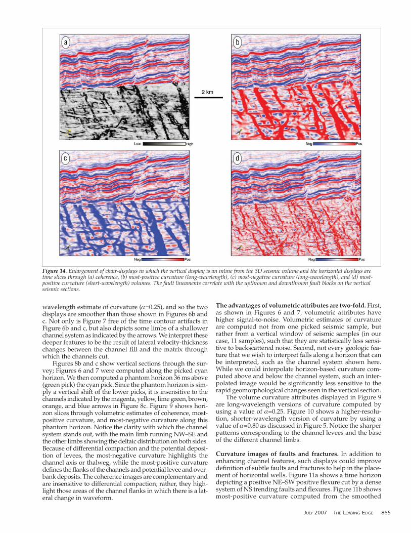
Figure 14. Enlargement of chair-displays in which the vertical display is an inline from the 3D seismic volume and the horizontal displays aretime slices through (a) coherence, (b) most-positive curvature (long-wavelength), (c) most-negative curvature (long-wavelength), and (d) most-positive curvature (short-wavelength) volumes. The fault lineaments correlate with the upthrown and downthrown fault blocks on the verticalseismic sections.

picked horizon, while Figures 11c and d show the corre-sponding horizon slices through long-wavelength (α=0.25)and short-wavelength (α=0.80) volumetric computations ofmost-positive curvature. Notice the artifacts on the horizon-based most-positive curvature display (indicated with theblue and green arrows) that are largely absent in the twovolumetric horizon slices.

Figure 12 shows the strat-cube displays of long-wave-length and short-wavelength versions of a fault/fracture sys-tem from Alberta. A strat-cube is a subvolume of seismicdata or its attributes, either bounded by two horizons whichmay not necessarily be parallel or covering seismic dataabove and/or below a given horizon. The surface displayedis close to 1550 ms. Notice that the long-wavelength displaygives the broad definition of such features, while the short-wavelength version depicts the finer definition of the indi-vidual lineaments.

Figure 13 shows another comparison of coherence andthe most-positive long-wavelength and short-wavelength

curvature. The lineaments seen in the short-wavelengthmost-positive curvature images (Figure 13c) are moredetailed than in the coherence (Figure 13a) and the long-wavelength most-positive curvature image (Figure 13b). Allattribute interpretations on time and horizon slices shouldbe validated through inspection of the vertical seismic data.Figure 14 shows enlarged views of the time slices fromcoherence, most-positive (both long-wavelength and high-resolution) and the long-wavelength most-negative curva-ture volumes intersecting a seismic inline. Notice that thered peaks (Figure 14b) on the fault lineaments (runningalmost NS) correlate with the upthrown signature on seis-mic. Similarly, the most-negative curvature time slice inter-secting the seismic inline (Figure 14c) shows the downthrownedges (highlighted in blue) on both sides of the faults.

Curvature attributes for well-log calibration. Figure 15ashows a time surface and an intersecting seismic line from a3D seismic volume from central-north British Columbia,

866 THE LEADING EDGE JULY 2007

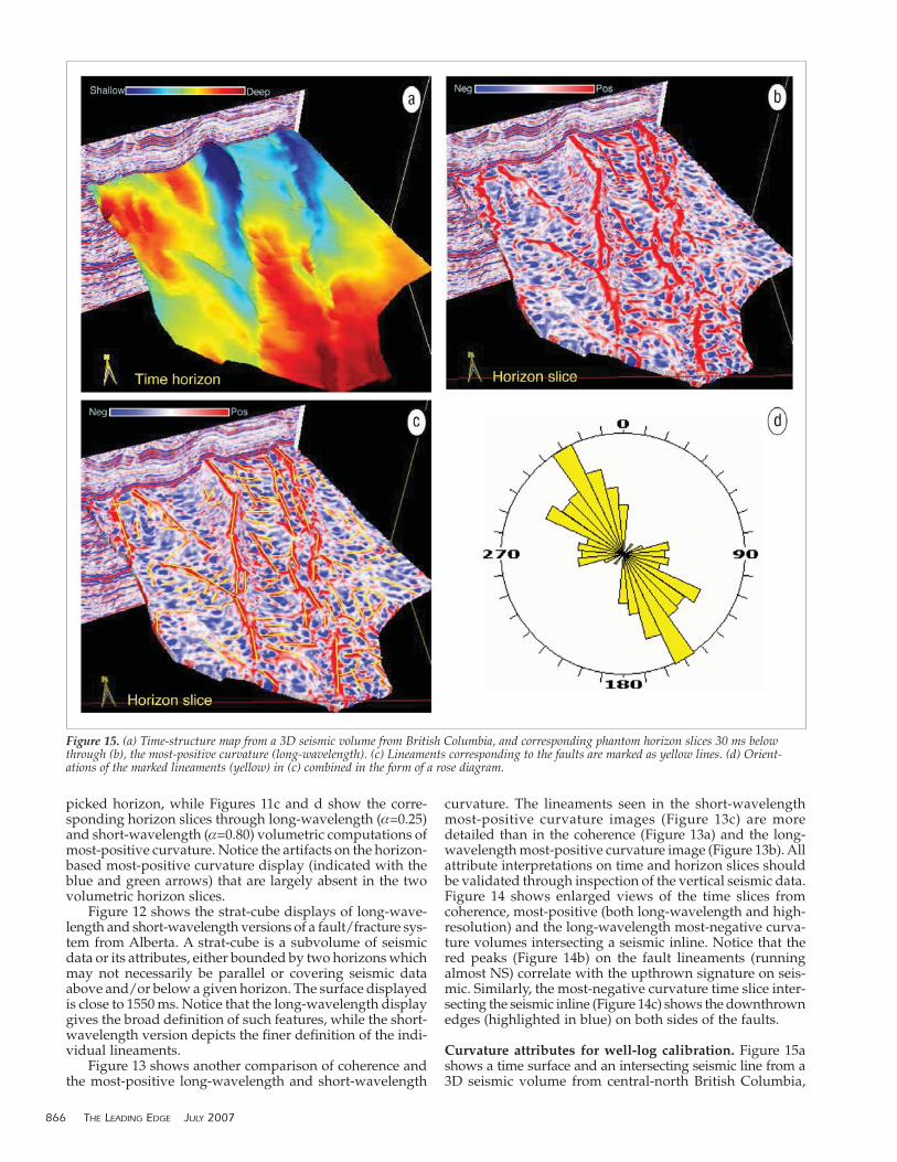
Figure 15. (a) Time-structure map from a 3D seismic volume from British Columbia, and corresponding phantom horizon slices 30 ms belowthrough (b), the most-positive curvature (long-wavelength). (c) Lineaments corresponding to the faults are marked as yellow lines. (d) Orient-ations of the marked lineaments (yellow) in (c) combined in the form of a rose diagram.

Canada. A number of faults can be seen on the vertical seis-mic section, and the main faults can be detected on the timesurface as well. Figure 15b shows a horizon slice extracted fromthe most-positive curvature volume at a level 30 ms belowthe horizon in Figure 15a. The individual lineaments corre-sponding to the two main faults running N–S as well as theirfracture offshoots have been tracked in yellow (Figure 15c).The orientations of these lineaments are displayed in a rosediagram (Figure 15d) which retains the color of the linea-ments. This rose diagram can be compared to a similar dia-gram obtained from image wells logs to gain confidence inseismic-to-well calibration. Once a favorable match is obtained,the interpretation of fault/fracture orientations and the thick-nesses over which they extend can be used with greater con-fidence for more quantitative reservoir analysis.

Conclusions. Curvature attributes provide important infor-mation above and beyond that derived from more commonlyused seismic attributes. Being second-order derivative mea-sures of surfaces, they are sensitive to noise. For time surfacespicked on noisy data, the noise problem can be addressed byiteratively running spatial filtering; for volume computationof attributes, structure-oriented filtering is satisfactory. Volumecurvature attributes reveal valuable information on fractureorientation and density in zones where seismic horizons arenot trackable. The orientations of the fault/fracture linea-ments interpreted on curvature displays can be combined inrose diagrams, which in turn can be compared with similardiagrams obtained from image wells logs to gain confidencein seismic-to-well calibration.

Suggested reading. “Multispectral estimates of reflector curva-ture and rotation” by Al-Dossary and Marfurt (GEOPHYSICS, 2006).“Improving curvature analyses of deformed horizons using scale-dependent filtering techniques” by Bergbauer et al. (AAPGBulletin, 2003). “Volume-based curvature analysis illuminatesfracture orientations” by Blumentritt (AAPG Annual Convention,2006). “Practical aspects of curvature computations from seismichorizons” by Chopra et al. (SEG 2006 Expanded Abstracts).“Curvature attribute applications to 3D seismic data” by Chopraand Marfurt (TLE, 2007). “Sunshading geophysical data usingfractional order horizontal gradients” by Cooper and Cowans(TLE, 2003). “Facies and curvature-controlled 3D fracture mod-els in a Cretaceous carbonate reservoir, Arabian Gulf” by Ericssonet al. (in Faulting, fault sealing, and fluid flow in hydrocarbon reser-voirs, Geological Society Special Publication 147, 1988). “Validatingseismic attributes: Beyond statistics” by Hart (TLE, 2002).“Improving seismic data for detailed structural interpretation”by Hesthammer (TLE, 1999). “Fast structural interpretation withstructure-oriented filtering” by Hoecker and Fehmers (TLE, 2002).“Detection of zones of abnormal strains in structures usingGaussian curvature analysis” by Lisle (AAPG Bulletin, 1994).“Edge-preserving smoothing and applications” by Luo et al.(TLE, 2002). “Robust estimates of reflector dip and azimuth” byMarfurt (GEOPHYSICS, 2006). “Kinematic evolution and fracture pre-diction of the Valle Morado structure inferred from 3D seismicdata, Salta province, northwest Argentina” by Massaferro et al.(AAPG Bulletin, 2003). “Curvature attributes and their applica-tion to 3D interpreted horizons” by Roberts (First Break, 2001).“Curvature attributes and seismic interpretation: Case studiesfrom Argentina basins” by Sigismondi and Soldo (TLE, 2003). TLE

Acknowledgments: We thank Arcis Corporation for permission to show thedata examples in Figures 3, 6, 7, 8, 9, 10, 11, and 15, and to publish thiswork.

Corresponding author: schopra@arcis.com

JULY 2007 THE LEADING EDGE 867