Volumetric Classification: Program kmeans3d

Attribute-Assisted Seismic Processing and Interpretation Page 1

Volumetric k-means clustering for 3D SEISMIC FACIES ANALYSIS – PROGRAM kmeans3d

Overview K-means (MacQueen, 1967) is perhaps the simplest clustering algorithm and is widely available in commercial interpretation software packages. kmeans3d is a volumetric seismic classification application that takes multiple seismic attributes as input, and generates a facies volume using k-means clustering. In kmeans3d, a user needs to specify the number of facies (clusters) to be generated, which is the k value in the k-means algorithm. Because the size of seismic data, in this implementation the software only takes a subset of data, extracted using a user specified decimation rate, to build a classifier, then apply this classifier to the whole 3D volume.

K-means is fast and easy to implement. Unfortunately, the clustering has no structure such that there is no relationship between the cluster numbering and the proximity of one cluster to another. This lack of organization can result in similar facies appearing in totally different colors, confusing the interpretation. Therefore, special care are needed when interpreting facies maps generated by k-means.

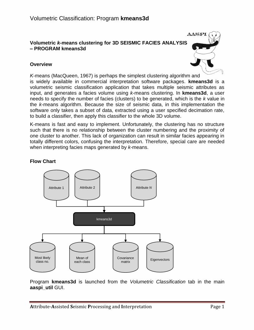
Flow Chart

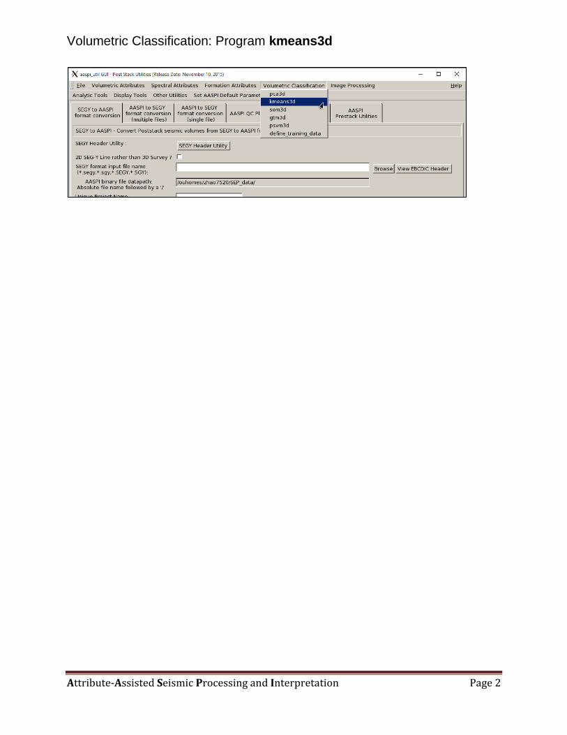
Program kmeans3d is launched from the Volumetric Classification tab in the main aaspi_util GUI.

kmeans3d

Most likely class no.

Attribute 1 Attribute 2 Attribute N …

Covariance matrix Eigenvectors Mean of

each class

Volumetric Classification: Program kmeans3d

Attribute-Assisted Seismic Processing and Interpretation Page 2

Volumetric Classification: Program kmeans3d

Attribute-Assisted Seismic Processing and Interpretation Page 3

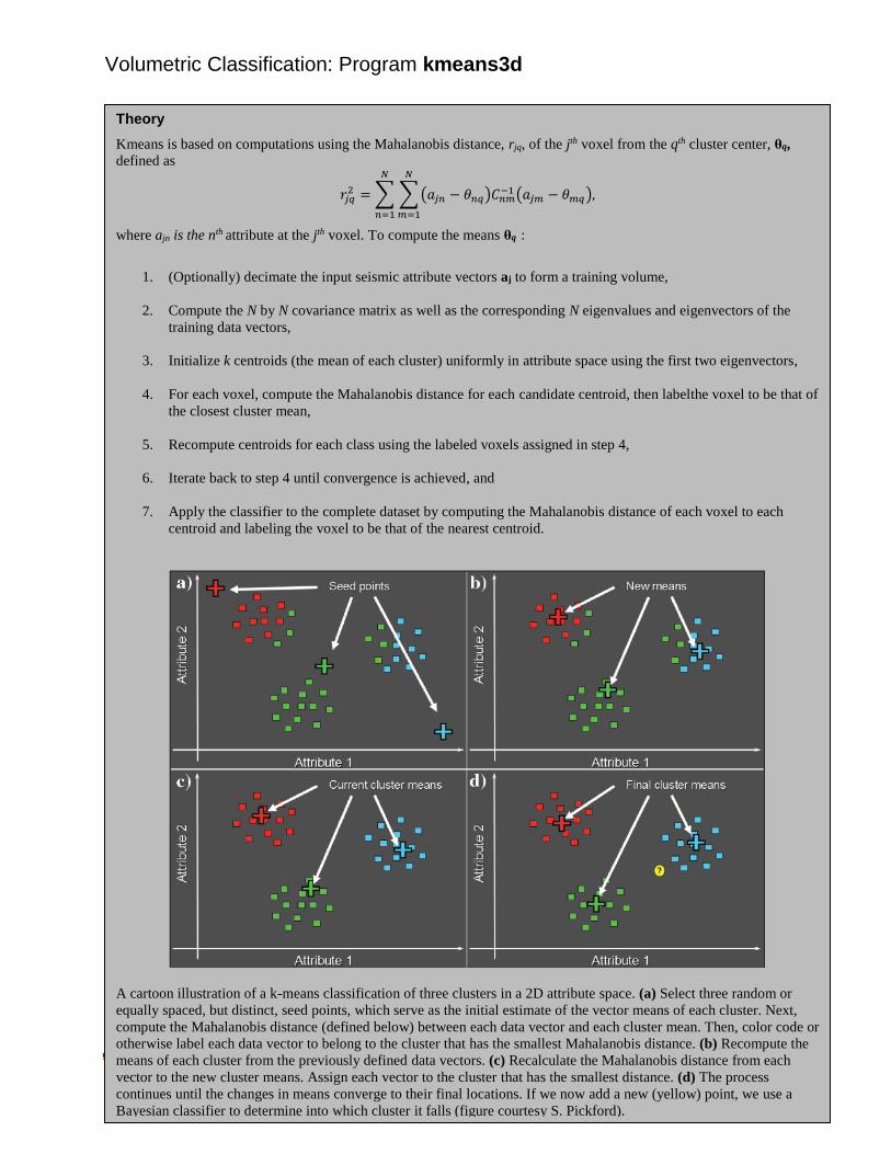
Theory

Kmeans is based on computations using the Mahalanobis distance, rjq, of the jth voxel from the qth cluster center, θq,

defined as

𝑟𝑗𝑞2 =∑ ∑(𝑎𝑗𝑛 − 𝜃𝑛𝑞)𝐶𝑛𝑚

−1 (𝑎𝑗𝑚 − 𝜃𝑚𝑞)

𝑁

𝑚=1

𝑁

𝑛=1

,

where ajn is the nth attribute at the jth voxel. To compute the means θq :

1. (Optionally) decimate the input seismic attribute vectors aj to form a training volume,

2. Compute the N by N covariance matrix as well as the corresponding N eigenvalues and eigenvectors of the

training data vectors,

3. Initialize k centroids (the mean of each cluster) uniformly in attribute space using the first two eigenvectors,

4. For each voxel, compute the Mahalanobis distance for each candidate centroid, then labelthe voxel to be that of

the closest cluster mean,

5. Recompute centroids for each class using the labeled voxels assigned in step 4,

6. Iterate back to step 4 until convergence is achieved, and

7. Apply the classifier to the complete dataset by computing the Mahalanobis distance of each voxel to each

centroid and labeling the voxel to be that of the nearest centroid.

A cartoon illustration of a k-means classification of three clusters in a 2D attribute space. (a) Select three random or

equally spaced, but distinct, seed points, which serve as the initial estimate of the vector means of each cluster. Next,

compute the Mahalanobis distance (defined below) between each data vector and each cluster mean. Then, color code or

otherwise label each data vector to belong to the cluster that has the smallest Mahalanobis distance. (b) Recompute the

means of each cluster from the previously defined data vectors. (c) Recalculate the Mahalanobis distance from each

vector to the new cluster means. Assign each vector to the cluster that has the smallest distance. (d) The process

continues until the changes in means converge to their final locations. If we now add a new (yellow) point, we use a

Bayesian classifier to determine into which cluster it falls (figure courtesy S. Pickford).

where the inversion of the covariance matrix, C, takes place prior to extracting the mnth element.

Volumetric Classification: Program kmeans3d

Attribute-Assisted Seismic Processing and Interpretation Page 4

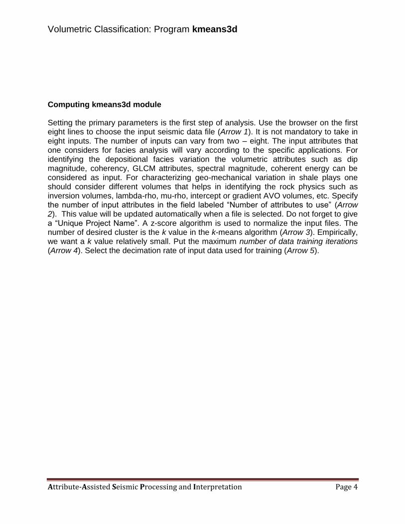
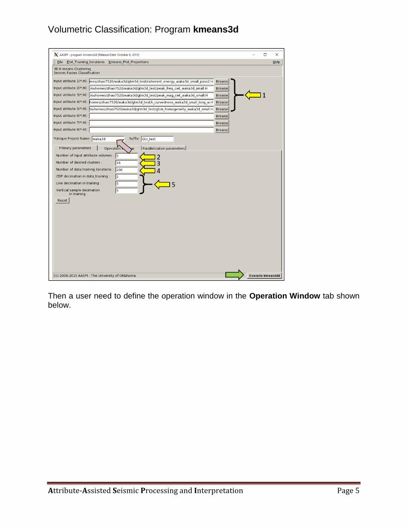
Computing kmeans3d module Setting the primary parameters is the first step of analysis. Use the browser on the first eight lines to choose the input seismic data file (Arrow 1). It is not mandatory to take in eight inputs. The number of inputs can vary from two – eight. The input attributes that one considers for facies analysis will vary according to the specific applications. For identifying the depositional facies variation the volumetric attributes such as dip magnitude, coherency, GLCM attributes, spectral magnitude, coherent energy can be considered as input. For characterizing geo-mechanical variation in shale plays one should consider different volumes that helps in identifying the rock physics such as inversion volumes, lambda-rho, mu-rho, intercept or gradient AVO volumes, etc. Specify the number of input attributes in the field labeled “Number of attributes to use” (Arrow 2). This value will be updated automatically when a file is selected. Do not forget to give a “Unique Project Name”. A z-score algorithm is used to normalize the input files. The number of desired cluster is the k value in the k-means algorithm (Arrow 3). Empirically, we want a k value relatively small. Put the maximum number of data training iterations (Arrow 4). Select the decimation rate of input data used for training (Arrow 5).

Volumetric Classification: Program kmeans3d

Attribute-Assisted Seismic Processing and Interpretation Page 5

Then a user need to define the operation window in the Operation Window tab shown below.

Volumetric Classification: Program kmeans3d

Attribute-Assisted Seismic Processing and Interpretation Page 6

Volumetric Classification: Program kmeans3d

Attribute-Assisted Seismic Processing and Interpretation Page 7

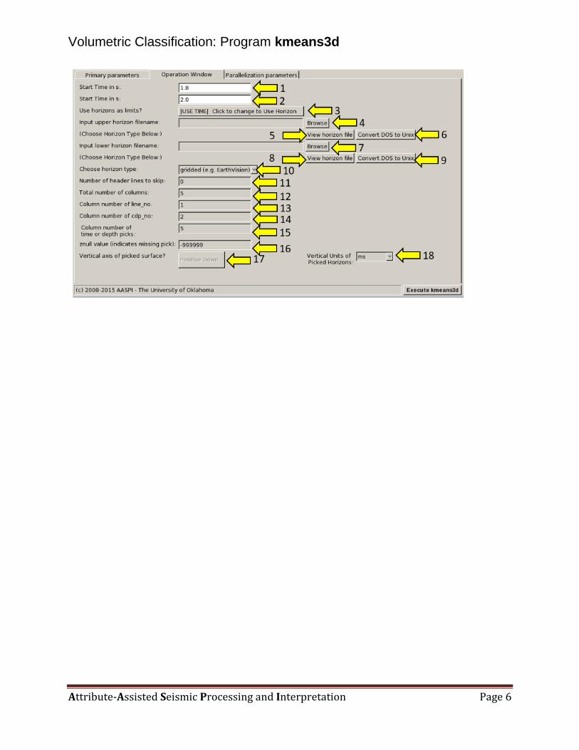
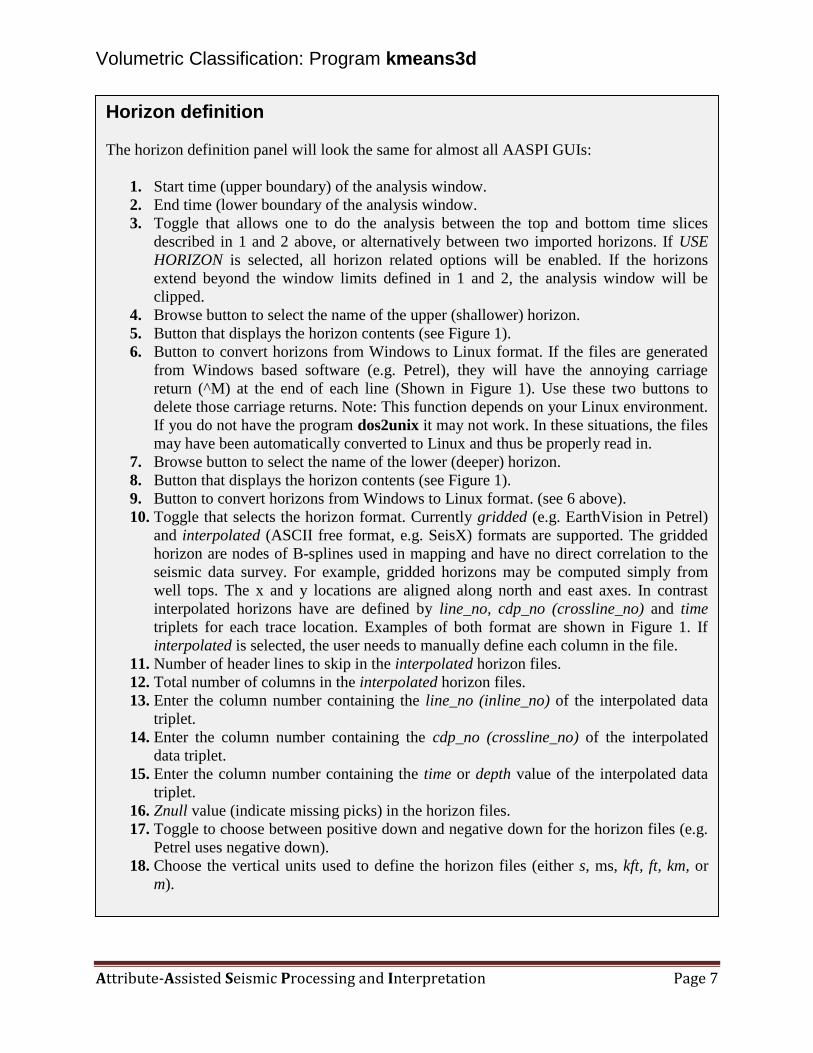
Horizon definition

The horizon definition panel will look the same for almost all AASPI GUIs:

1. Start time (upper boundary) of the analysis window.

2. End time (lower boundary of the analysis window.

3. Toggle that allows one to do the analysis between the top and bottom time slices

described in 1 and 2 above, or alternatively between two imported horizons. If USE

HORIZON is selected, all horizon related options will be enabled. If the horizons

extend beyond the window limits defined in 1 and 2, the analysis window will be

clipped.

4. Browse button to select the name of the upper (shallower) horizon.

5. Button that displays the horizon contents (see Figure 1).

6. Button to convert horizons from Windows to Linux format. If the files are generated

from Windows based software (e.g. Petrel), they will have the annoying carriage

return (^M) at the end of each line (Shown in Figure 1). Use these two buttons to

delete those carriage returns. Note: This function depends on your Linux environment.

If you do not have the program dos2unix it may not work. In these situations, the files

may have been automatically converted to Linux and thus be properly read in.

7. Browse button to select the name of the lower (deeper) horizon.

8. Button that displays the horizon contents (see Figure 1).

9. Button to convert horizons from Windows to Linux format. (see 6 above).

10. Toggle that selects the horizon format. Currently gridded (e.g. EarthVision in Petrel)

and interpolated (ASCII free format, e.g. SeisX) formats are supported. The gridded

horizon are nodes of B-splines used in mapping and have no direct correlation to the

seismic data survey. For example, gridded horizons may be computed simply from

well tops. The x and y locations are aligned along north and east axes. In contrast

interpolated horizons have are defined by line_no, cdp_no (crossline_no) and time

triplets for each trace location. Examples of both format are shown in Figure 1. If

interpolated is selected, the user needs to manually define each column in the file.

11. Number of header lines to skip in the interpolated horizon files.

12. Total number of columns in the interpolated horizon files.

13. Enter the column number containing the line_no (inline_no) of the interpolated data

triplet.

14. Enter the column number containing the cdp_no (crossline_no) of the interpolated

data triplet.

15. Enter the column number containing the time or depth value of the interpolated data

triplet.

16. Znull value (indicate missing picks) in the horizon files.

17. Toggle to choose between positive down and negative down for the horizon files (e.g.

Petrel uses negative down).

18. Choose the vertical units used to define the horizon files (either s, ms, kft, ft, km, or

m).

Volumetric Classification: Program kmeans3d

Attribute-Assisted Seismic Processing and Interpretation Page 8

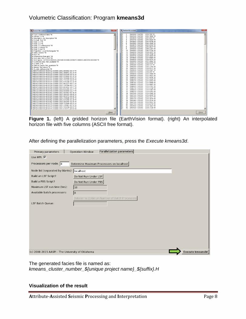
Figure 1. (left) A gridded horizon file (EarthVision format). (right) An interpolated horizon file with five columns (ASCII free format). After defining the parallelization parameters, press the Execute kmeans3d.

The generated facies file is named as: kmeans_cluster_number_${unique project name}_${suffix}.H Visualization of the result

Volumetric Classification: Program kmeans3d

Attribute-Assisted Seismic Processing and Interpretation Page 9

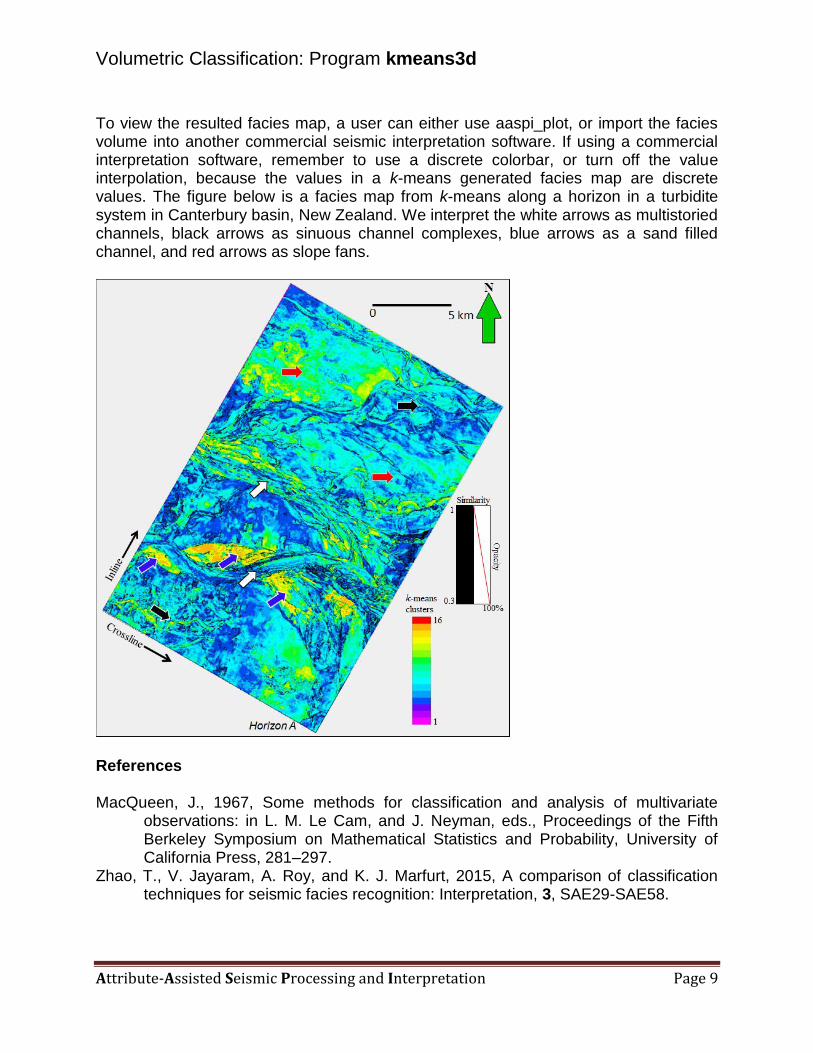
To view the resulted facies map, a user can either use aaspi_plot, or import the facies volume into another commercial seismic interpretation software. If using a commercial interpretation software, remember to use a discrete colorbar, or turn off the value interpolation, because the values in a k-means generated facies map are discrete values. The figure below is a facies map from k-means along a horizon in a turbidite system in Canterbury basin, New Zealand. We interpret the white arrows as multistoried channels, black arrows as sinuous channel complexes, blue arrows as a sand filled channel, and red arrows as slope fans.

References

MacQueen, J., 1967, Some methods for classification and analysis of multivariate

observations: in L. M. Le Cam, and J. Neyman, eds., Proceedings of the Fifth Berkeley Symposium on Mathematical Statistics and Probability, University of California Press, 281–297.

Zhao, T., V. Jayaram, A. Roy, and K. J. Marfurt, 2015, A comparison of classification techniques for seismic facies recognition: Interpretation, 3, SAE29-SAE58.