Embed Size (px)
Citation preview

Volume, Volatility and Public News Announcements∗
Tim Bollerslev,† Jia Li,‡ and Yuan Xue§
June 22, 2016
Abstract
We provide new empirical evidence for the way in which financial markets process information.Our results are based on high-frequency intraday data along with new econometric techniques formaking inference on the relationship between trading intensity and spot volatility around publicnews announcements. Consistent with the predictions derived from a theoretical model in whichinvestors agree to disagree, our estimates for the intraday volume-volatility elasticity around themost important news announcements are systematically below unity. Our elasticity estimatesalso decrease significantly with measures of disagreements in beliefs, economic uncertainty, andtextual-based sentiment, further highlighting the key role played by differences-of-opinion.
Keywords: Differences-of-opinion; high-frequency data; jumps; macroeconomic news announce-ments; trading volume; stochastic volatility; economic uncertainty; textual sentiment.
JEL classification: C51, C52, G12.
∗We would like to thank Joel Hasbrouck, Neil Shephard, George Tauchen, Brian Weller, Dacheng Xiu, and seminarparticipants at Duke University for their helpful comments. Bollerslev and Li gratefully acknowledge support fromCREATES funded by the Danish National Research Foundation (DNRF78) and the NSF (SES-1326819), respectively.†Department of Economics, Duke University, Durham, NC 27708; NBER; CREATES; e-mail: [email protected].‡Department of Economics, Duke University, Durham, NC 27708; e-mail: [email protected].§Department of Economics, Duke University, Durham, NC 27708; e-mail: [email protected].

1 Introduction
Trading volume and return volatility in financial markets typically, but not always, move in tandem.
By studying the strength of this relationship around important public news announcements, we
shed new light on the way in which financial markets process new information and the key role
played by differences-of-opinion among investors. Our empirical investigations rely critically on the
use of high-frequency intraday data and new econometric procedures explicitly designed to deal
with complications that arise in the high-frequency data setting.
An extensive empirical literature has documented the existence of a strong contemporaneous
relation between trading volume and volatility; see Karpoff (1987) for a survey of some of the
earliest empirical evidence. The mixture-of-distributions hypothesis (MDH), originally developed
by Clark (1973) and later extended by Tauchen and Pitts (1983) and Andersen (1996) among others,
provides a possible explanation for this empirical relationship based on the idea of a common news
arrival process driving both the magnitude of returns and trading volume. The MDH, however,
remains silent about the underlying economic mechanisms that link the actual trades and price
adjustments to the news.
Meanwhile, a variety of equilibrium-based economic models have also been developed to help
understand how prices and volume respond to new information. This includes the rational-
expectations type models of Kyle (1985) and Kim and Verrecchia (1991) among many others,
in which investors agree on the interpretation of the news, but their information sets differ. Al-
though this class of models is able to account for the on-average positive correlation between volume
and volatility observed empirically, the models are unable to explain the occurrence of abnormally
large trading volumes that occasionally occur together with returns close to zero. Instead, models
that feature differences-of-opinion, including those by Harrison and Kreps (1978), Harris and Raviv
(1993), Kandel and Pearson (1995), Scheinkman and Xiong (2003) and Banerjee and Kremer (2010)
among others, in which investors agree to disagree, may help explain this oft observed empirical
phenomenon. In the differences-of-opinion class of models, the investors’ interpretation of the news
and their updated valuations of the assets do not necessarily coincide, thus allowing for the possibil-
ity of relatively small equilibrium price changes accompanied by relatively large aggregate trading
volumes.
Most of the existing empirical evidence related to the economic models discussed above, and
1

the volume-volatility relationship in particular, has been based on daily or coarser frequency data.1
Meanwhile, another more recent strand of literature has emphasized the advantages of the use of
high-frequency intraday data for more accurately identifying “jumps” and studying the way in which
financial prices respond to public news announcements; see, for example, Andersen et al. (2003),
Andersen et al. (2007), Lee and Mykland (2008) and Lee (2012).2 This naturally suggests that
by “zooming in” and analyzing how not only prices but also trading volume and volatility evolve
around important news announcements, a deeper understanding of the economic mechanisms at
work and the functioning of markets may be forthcoming.
Set against this background, we provide new empirical evidence on the volume-volatility rela-
tionship around various macroeconomic news announcements based on high-frequency one-minute
data for the S&P 500 aggregate market portfolio. We begin by documenting the occurrence of large
increases in trading volume intensity around Federal Open Market Committee (FOMC) meetings
without accompanying large price jumps. As noted above, this presents a challenge for models in
which investors rationally update their beliefs based on the same interpretation of the news, and
instead points to the importance of models allowing for disagreements or, differences-of-opinion,
among investors.
To help further explore this thesis and guide our more in-depth empirical investigations, we
derive an explicit expression for the elasticity of expected trading volume with respect to price
volatility within the Kandel and Pearson (1995) differences-of-opinion model. We purposely focus
our analysis on the elasticity as it may be conveniently estimated with high-frequency data and,
importantly, has a clear economic interpretation in terms of model primitives. In particular, we
show theoretically that the volume-volatility elasticity is monotonically decreasing in a well-defined
measure of relative disagreement. Moreover, the elasticity is generally below one and reaches its
upper bound of unity only in the benchmark case without disagreement.
The theoretical model underlying these predictions is inevitably stylized, focussing exclusively
on the impact of public news announcements. As such, the theory mainly speaks to the “abnormal”
movements in volume and volatility observed around these news events. To identify the abnormal
movements, and thus help mitigate the effects of other confounding forces, we rely on the “jumps”
in the volume intensity and volatility around the news announcements. Our estimation of the
jumps is based on the differences between the post- and pre-event levels of the instantaneous
1One notable exception is Chaboud et al. (2008), who document large trading volume in the foreign exchangemarket in the minutes immediately before macroeconomic announcements, even when the announcements are in linewith market expectations and the actual price changes are small.
2Related to this, Savor and Wilson (2013) also document higher average excess market returns on days withimportant macroeconomic news releases compared to non-announcement days.
2

volume intensity and volatility, which we recover nonparametrically using high-frequency data.
Even though the differencing step used in identifying the jumps effectively removes low-frequency
dynamics in the volatility and volume series (including daily and lower frequency trending behavior)
that might otherwise confound the estimates, the jump estimates are still affected by the well-
documented strong intraday periodic patterns that exist in both volume and volatility (for some
of the earliest empirical evidence, see Wood et al., 1985; Jain and Joh, 1988). In an effort to
remove this additional confounding influence we apply a second difference with respect to a control
group of non-announcement days. The resulting “doubly-differenced” jump estimates in turn serve
as our empirical analogues of the abnormal volume and volatility movements that we use in our
regression-based analysis of the theoretical predictions.
In its basic form, our empirical regression strategy may be viewed as a Differences-in-Differences
(DID) type estimator, as commonly used in empirical microeconomic studies; see, for example,
Ashenfelter and Card (1985). However, our setup is distinctly different from conventional settings,
and the usual justification for the use of DID regressions does not apply in the high-frequency data
setting. Correspondingly, our new econometric procedures and the justification thereof entail two
important distinctions. Firstly, to accommodate the strong dynamic dependencies in the volatility
and volume intensity, we provide a rigorous theoretical justification based on a continuous-time
infill asymptotic framework allowing for essentially unrestricted non-stationarity. Secondly, we
provide an easy-to-implement local i.i.d. bootstrap method for conducting valid inference. By
randomly resampling only locally in time (separately before and after each announcement), the
method provides a simple solution to the issue of data heterogeneity, which otherwise presents a
key complication for bootstrapping in the high-frequency data setting (see, e.g., Goncalves and
Meddahi, 2009).
Our actual empirical findings are closely in line with the theoretical predictions derived from the
Kandel and Pearson (1995) model and the differences-of-opinion class of models more generally.
In particular, we first document that the estimated volume-volatility elasticity around FOMC
announcements is significantly below unity. This finding carries over to other important intraday
public news announcements closely monitored by market participants. Interestingly, the volume-
volatility elasticity estimates are lower for announcements that are released earlier in the monthly
news cycle (see Andersen et al., 2003), such as the ISM Manufacturing Index and the Consumer
Confidence Index, reflecting the importance of timing across the announcements and the effect of
learning.
Going one step further, we show that the intraday volume-volatility elasticity around news
3

announcements decreases significantly in response to increases in measures of dispersions-in-beliefs
(based on the survey of professional forecasters as in, e.g., Van Nieuwerburgh and Veldkamp, 2006)
and economic uncertainty (based on the economic policy uncertainty index of Baker et al., 2015).
This again corroborates our theoretical predictions and the key role played by differences-of-opinion.
Our more detailed analysis of FOMC announcements, in which we employ an additional textual-
based measure for the negative sentiment in the accompanying FOMC statements (based on the
methodology of Loughran and McDonald, 2011), further underscores the time-varying nature of
the high-frequency volume-volatility relationship and the way in which the market processes new
information: when the textual sentiment in the FOMC statement is more negative, the relative
disagreement among investors also tends to be higher, pushing down the volume-volatility elasticity.
The rest of the paper is organized as follows. Section 2 presents the basic economic argu-
ments and theoretical model that guide our empirical investigations. Section 3 describes the high-
frequency intraday data and news announcements used in our empirical analysis. To help further
motivate and set the stage for our more detailed subsequent empirical investigations, Section 4
discusses some preliminary findings specifically related to FOMC announcements. Section 5 de-
scribes the new high-frequency inference procedures that we rely on for our more in-depth empirical
analysis. Section 6 presents our main empirical findings based on the full set of news announce-
ments, followed by our more detailed analysis of FOMC announcements. Section 7 concludes.
Technical details concerning the new econometric inference procedure are provided in Appendix A.
Appendix B contains further data descriptions. Additional empirical results and robustness checks
are relegated to a (not-for-publication) supplemental appendix.
2 Theoretical motivation
We rely on the theoretical volume-volatility relations derived from the differences-of-opinion model
of Kandel and Pearson (1995) to help guide our empirical investigations. We purposely focus on
a simplified version of the model designed to highlight the specific features that we are after, and
the volume-volatility elasticity around news arrivals in particular. To contrast the differences-
of-opinion and rational-expectations types of models, we also briefly outline the corresponding
empirical implications from a simplified version of the Kim and Verrecchia (1991) model. We begin
by discussing the basic setup and assumptions.
4

2.1 New information and differences-of-opinion
Following Kandel and Pearson (1995), henceforth KP, we assume that a continuum of traders trade
a risky asset and a risk-free asset in a competitive market. The random payoff of the risky asset,
denoted u, is unknown to the traders. The risk-free rate is normalized to be zero. The traders’
utility functions have constant absolute risk aversion with risk tolerance r. Each trader receives a
noisy private signal about the payoff of the risky asset. Conditional on u, the private signals are
independent and normally distributed. There are only two types of traders, i ∈ 1, 2, with the
proportion of type 1 traders denoted α. The precision of type-i trader’s signal is si.
The public signal is u+ ε, where the noise term ε is normally distributed. After observing the
public signal, the traders update their beliefs about u and optimally re-balance their positions. The
key feature of the KP model is that the two types of traders agree to disagree on how to interpret
the public signal when updating their beliefs about the asset value: type i traders believe that
ε is drawn from the N(µi, h−1) distribution. Differences-of-opinion regarding the public signal is
present among the traders when µ1 6= µ2.
Following KP it is possible to show that in equilibrium3
Volume = |β0 + β1 · Price Change| , (2.1)
where
β0 = rα (1− α)h (µ1 − µ2) , β1 = rα (1− α) (s1 − s2) . (2.2)
We remark that the coefficient β0 is directly associated with the degree of differences-of-opinion (i.e.,
µ1 − µ2), whereas β1 depends on the dispersion in the precisions of prior beliefs. Both coefficients
are increasing in the degree of risk tolerance.
By way of contrast, we also consider the rational-expectations model of Kim and Verrecchia
(1991), in which rational traders agree on the interpretation of the public signal. In this setting,
only if the equilibrium price changes in response to the public signal, will the optimal positions of
the traders change. In particular, in parallel to the expression above it is possible to show that4
Volume = |β1 · Price Change| . (2.3)
Even though the economic mechanism of Kim and Verrecchia (1991) differs from that of the KP
model, the empirical implications from equation (2.3) are obviously nested in equation (2.1) with
β0 = 0, that is, the case without differences-of-opinion.
3See equation (5) in Kandel and Pearson (1995).4See Proposition 2 of Kim and Verrecchia (1991).
5
2.2 Expected volume and volatility
The implication of the KP model for the relationship between price adjustment and trading volume
in response to new information is succinctly summarized by equations (2.1) and (2.2). These
equations, however, depict an exact functional relationship between (observed) random quantities.
A weaker, but empirically more realistic, implication can be obtained by thinking of this equilibrium
relationship as only holding “on average.” Moment conditions corresponding to the stochastic
version (2.1) formally capture this idea.
Specifically, let m(σ) denote the expected volume as a function of the volatility σ (i.e., the
standard deviation of price change). Assuming that the price changes are normally distributed
with mean zero and standard deviation σ, it follows by direct integration of (2.1) that
m (σ) =
√2
π|β1|σ exp
(− β2
0
2β21σ
2
)+ |β0|
(2Φ
(|β0||β1|σ
)− 1
), (2.4)
where Φ denotes the cumulative distribution function of the standard normal distribution.5 The
expected volume m(σ) depends on σ and the (β0, β1) coefficients in a somewhat complicated fashion.
However, it is straightforward to show that m(σ) is increasing and convex in σ.
In order to gain further insight regarding this (expected) volume-volatility relationship, Figure
1 illustrates how the m(σ) function varies with the “disagreement coefficient” β0. Locally, when
the volatility σ is close to zero, the expected volume is positive if and only if the opinions of the
traders differ (i.e., µ1 6= µ2). Globally, as β0 increases (from the bottom to the top curves in the
figure), the equilibrium relationship between the expected volume and volatility “flattens out.”
It is useful for our analysis below to further quantify this global feature in terms of the elasticity
of m(σ) with respect to σ. We will denote this elasticity by E , and refer to it as the volume-volatility
elasticity for short. A straightforward calculation yields
E ≡ ∂m(σ)/m(σ)
∂σ/σ=
1
1 + ψ (γ/σ), (2.5)
where
γ ≡ |β0||β1|
=h |µ1 − µ2||s1 − s2|
, (2.6)
and the function ψ is defined by ψ (x) ≡ x (Φ (x)− 1/2) /φ (x), with φ being the density function
of the standard normal distribution. The function ψ is strictly increasing on [0,∞), with ψ(0) = 0
and limx→∞ ψ(x) =∞.
5Similarly, for the Kim and Verrecchia (1991) rational-expectations type model and the expression in (2.3), m(σ) =√2|β1|σ/
√π.
6

Figure 1: Equilibrium volume-volatility relations
0 0.2 0.4 0.6 0.8 1 1.2 1.4 1.6 1.8 20
0.5
1
1.5
2
m
σ
Notes: The figure shows the equilibrium relationship between expected trading volume m and price volatility σ inthe Kandel–Pearson model for various levels of disagreement, ranging from β0 = 0 (bottom) to 0.5, 1 and 1.5 (top).β1 is fixed at one in all of the graphs.
The expressions in (2.5) and (2.6) embody two important features of the volume-volatility
elasticity that we use to guide our empirical analysis. Firstly, E ≤ 1 with the equality and an
elasticity of unity obtaining if and only if γ = 0. Secondly, E only depends on and is decreasing in
γ/σ. This second feature provides a clear economic interpretation of the volume-volatility elasticity
E : it is low when differences-in-opinion is relatively high, and vice versa, with γ/σ serving as the
relative measure of the differences-of-opinion. This relative measure is higher when traders disagree
more on how to interpret the public signal (i.e., larger |µ1 − µ2|) and with more confidence (i.e.,
larger h), relative to the degree of asymmetric private information (i.e., |s1 − s2|) and the overall
price volatility (i.e., σ).
In our empirical investigations discussed below, we seek to directly quantify these relations based
on intraday high-frequency transaction data around well-defined public news announcements, along
with various proxies for the heterogeneity in beliefs and economic uncertainty associated with the
news events. We turn next to a discussion of the data that we use in doing so.
7

Table 1: Summary statistics of high-frequency price returns and volume data
Mean Min 1% 25% 50% 75% 99% Max
Return (percent) 0.000 -2.014 -0.149 -0.021 0.000 0.021 0.149 2.542
Volume (1,000 shares) 289.5 0.0 2.4 55.4 147.6 350.7 2005 31153
Notes: The table reports summary statistics of the one-minute returns and one-minute trading vol-umes for the SPY ETF during regular trading hours from April 10, 2001 to September 30, 2014.
3 Data description and summary statistics
Our empirical investigations are based on high-frequency intraday transaction prices and trading
volume, together with precisely timed macroeconomic news announcements. We describe our data
sets in turn.
3.1 High-frequency market prices and trading volume
Our primary data is comprised of intraday transaction prices and trading volume for the S&P
500 index ETF (ticker: SPY). In some of our robustness checks we also employ high-frequency
data of an ETF tracking the Dow Jones Industrial Average (ticker: DIA). All data are obtained
from the TAQ database. The sample covers all regular trading days from April 10th, 2001 through
September 30th, 2014. The raw data are cleaned and sampled at the one-minute frequency following
the procedures detailed in Brownlees and Gallo (2006) and Barndorff-Nielsen et al. (2009). In total,
there are 1,315,470 observations of one-minute return and trading volume.
Summary statistics for the SPY returns and trading volumes (number of shares) are reported
in Table 1. Consistent with prior empirical evidence (see, e.g., Bollerslev and Todorov (2011)), the
high-frequency one-minute returns appear close to be symmetrically distributed. The one-minute
volume series, on the other hand, is highly skewed to the right, with occasionally very large values.
To highlight the general dynamic dependencies inherent in the data, Figure 2 plots the daily
logarithmic trading volume (constructed by summing the one-minute trading volumes over each of
the different days) and the logarithmic daily realized volatilities (constructed as the sum of squared
one-minute returns over each of the days in the sample). As the figure shows, both of the daily
series vary in a highly predictable fashion. The volume series, in particular, seems to exhibit an
upward trend over the first half of the sample, but then levels off over the second half. Meanwhile,
consistent with the extensive prior empirical evidence discussed above, there are strong dynamic
commonalities evident in the two series.
In addition to the strong intertemporal dynamic dependencies, the volume and volatility series
8

Figure 2: Time series of volume and volatility
2002 2003 2004 2005 2006 2007 2008 2009 2010 2011 2012 2013 20140
2
4
6
8
2002 2003 2004 2005 2006 2007 2008 2009 2010 2011 2012 2013 20141
2
3
4
5
Notes: The figure shows the daily logarithmic trading volume (top panel) and logarithmic realized volatility (bottompanel) for the SPY ETF. The daily volume is constructed by accumulating the intraday volume. The daily realizedvolatility is constructed as the sum of one-minute squared returns over the day.
also exhibit strong intraday patterns. To illustrate this, Figure 3 plots the square-root of the one-
minute squared returns averaged across each minute-of-the-day (as an estimate for the volatility
over that particular minute) and the average trading volume over each corresponding minute. In
order to prevent abnormally large returns and volumes from distorting the picture, we only include
non-announcement days that are discussed in Section 3.2 below. Consistent with the evidence in
the extant literature, there is a clear U-shaped pattern in the average volatility and trading activity
over the active part of the trading day.6
3.2 Macroeconomic news announcements
The Economic Calendar Economic Release section in Bloomberg includes the date and exact within
day release time for over one-hundred regularly scheduled macroeconomic news announcements.
Most of these announcements occur before the market opens or after it closes. We purposely focus
on announcements that occur during regular trading hours only.7 All-in-all, this leaves with 21
6See Wood et al. (1985), Harris (1986), Jain and Joh (1988), Baillie and Bollerslev (1990), and Andersen andBollerslev (1997) for some of the earliest empirical evidence on the intraday patterns in volatility and volume.
7To ensure that there is a 30-minute pre-event (resp. post-event) window before (resp. after) each announcement,we exclude announcements that are released during the first and the last 30 minutes of the trading day.
9

Figure 3: Intraday patterns of volatility and volume
12:00 15:0010
15
20
25
30
35
Data
Fitted Line
12:00 15:000
2
4
6
8
10
12
14x 10
5
Data
Fitted Line
Notes: The figure shows the intraday volatility for the SPY ETF (left panel) constructed as the square root ofthe one-minute squared returns averaged across all non-announcement days, along with the best quadratic fit. Theintraday trading volume for the SPY ETF (right panel) is similarly averaged across all non-announcement days.
different indicators for a total of 2,130 intraday public news announcements over the April 10, 2001
to September 30, 2014 sample period.
We identify four types of important announcements that comprise of the FOMC rate decision
(FOMC), ISM Manufacturing Index (ISMM), ISM Non-Manufacturing Index (ISMNM), and the
Consumer Confidence (CC) Index, based on prior empirical evidence.8 Table 2 provides the typical
release times and the number of releases over the sample for each of these important indicators.
The remaining announcements are categorized as Others, a full list of which is provided in Table
B.1 in Appendix B.
4 A preliminary analysis of FOMC announcements
To set the stage for our more in-depth subsequent empirical investigations, we begin by presenting a
set of simple summary statistics and illustrative figures related to the volume-volatility relationship
around FOMC announcements. We focus our preliminary analysis on FOMC announcements,
because these are arguably among the most important public news announcements that occur
during regular trading hours.9
8See, for example, Andersen et al. (2003), Boudt and Petitjean (2014), Jiang et al. (2011) and Lee (2012).9The reaction of market prices to FOMC announcements has been extensively studied in the recent literature; see,
for example, Johnson and Paye (2015) and many references therein.
10

Table 2: Macroeconomic news announcements
No.Obs. Time Source
FOMC 109 14:15† Federal Reserve Board
ISM Manufacturing (ISMM) 160 10:00 Institute of Supply Management
ISM Non-Manufacturing (ISMNM) 158 10:00 Institute of Supply Management
Consumer Confidence (CC) 160 10:00 Conference Board
Other Indicators (Others) 1682 Varies
Notes: The table reports the total number of observations, release time, and data sourcefor each of the news announcements over the April 10, 2001 to September 30, 2014 sample.†The exact times mostly vary from 14:00 to 14:15.
For each announcement, let τ denote the pre-scheduled announcement time (typically at 14:15
EST). The time τ is naturally associated with the integer i(τ) such that τ = (i(τ) − 1)∆n, where
∆n = 1 minute is the sampling interval of our intraday data. We define the event window as
((i(τ)− 1) ∆n, i(τ)∆n]. Further, we define the pre-event (resp. post-event) window to be the
kn-minute period immediately before (resp. after) the event window. We denote the return and
trading volume over the jth intraday time-interval ((j − 1)∆n, j∆n] by rj and Vj∆n , respectively.
The volume intensity m (i.e., the instantaneous mean volume) and the spot volatility σ before and
after the announcement, denoted by mτ−, mτ , στ− and στ , respectively, may then be estimated by
mτ− ≡ 1kn
∑knj=1 V(i(τ)−j)∆n
, mτ ≡ 1kn
∑knj=1 V(i(τ)+j)∆n
,
στ− ≡√
1kn∆n
∑knj=1 r
2i(τ)−j , στ ≡
√1
kn∆n
∑knj=1 r
2i(τ)+j .
(4.1)
These estimators are nonparametric, in the sense that they use data in local windows around
the event time, where the window size kn plays the role of the bandwidth parameter in usual
nonparametric analysis. Under some standard technical assumptions that we detail in Appendix
A, the validity of these nonparametric estimators can be justified. We set kn = 30 that corresponds
to a 30-minute window.
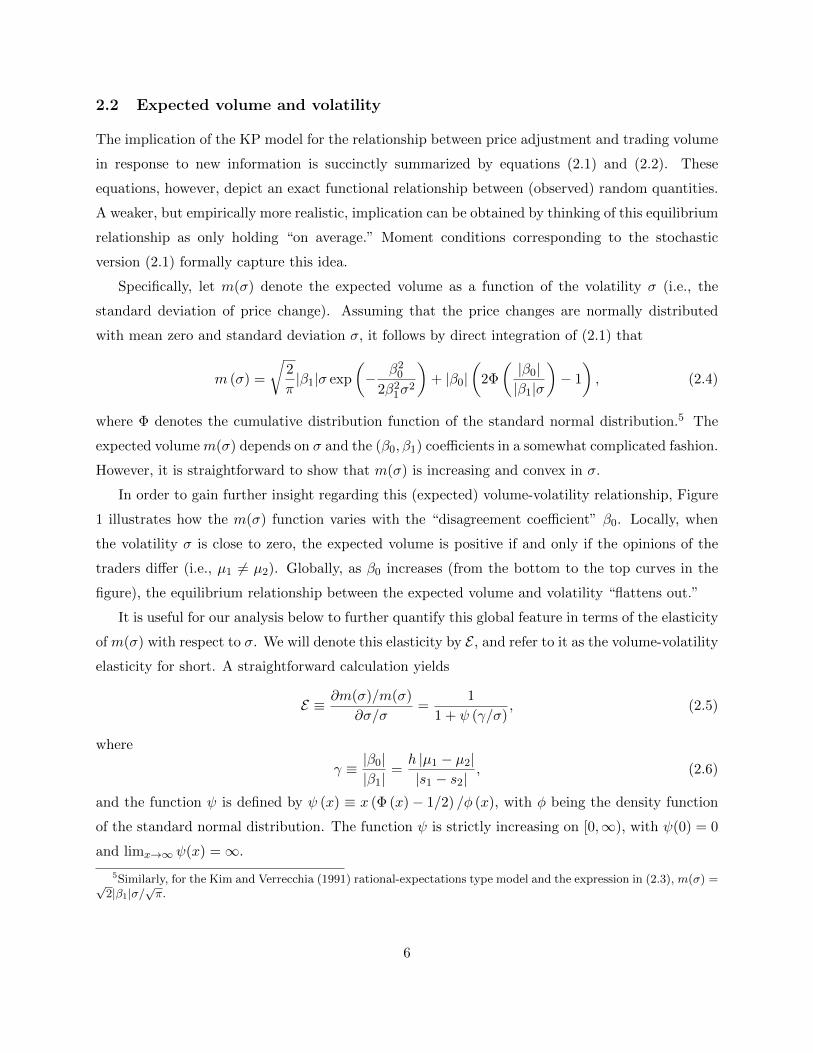
Figure 4 plots the resulting time series of estimated logarithmic volume intensities (top panel)
and logarithmic spot volatilities (bottom panel) before and after the FOMC announcements.10 We
observe marked bursts in the trading volume following each FOMC announcements, accompanied by
positive jumps in the volatility. These jumps in the volume intensity and volatility are economically
10The logarithmic transform is naturally motivated by our interest in the volume-volatility elasticity derived inSection 2.2. The log-transformation also helps reduce the heteroskedasticity in both series. The heteroskedasticityin the spot volatility estimates is directly attributable to estimation errors. Formally, the standard error of the στestimate equals στ/
√2kn, so that by the delta-method the standard error of log(στ ) equals the constant 1/
√2kn. In
addition, the logarithm effectively transforms the salient multiplicative trend in the volume series over the first halfof the sample to an additive trend, which as seen in Figure 2 is close to linear in time.
11
Figure 4: Volume and volatility around FOMC announcements
2002 2003 2004 2005 2006 2007 2008 2009 2010 2011 2012 2013 20148
10
12
14
16
18Log Volume Intensity
Pre−eventPost−event
2002 2003 2004 2005 2006 2007 2008 2009 2010 2011 2012 2013 2014−2
−1
0
1
2
3Log Spot Volatility
Notes: The figure plots the log-volume intensity (top panel) and log-volatility (bottom panel) around FOMCannouncements. The volume intensity and volatility are calculated using equation (4.1) with kn = 30.
large, with average jump sizes (in log) of 1.41 and 1.09, respectively.11 This suggests that traders
revise their beliefs about the stock market differently upon seeing the FOMC release. It is, of course,
possible that traders have asymmetric private information about the overall market, although it
seems much more likely that any differences are attributed to the traders’ different interpretation
of the news.12
In order to further buttress the importance of differences-of-opinion among investors, we con-
sider two additional empirical approaches. Firstly, as discussed in Section 2.1, if all investors agreed
on the interpretation of the FOMC announcements, the trading volumes observed around the news
releases should be approximately proportional to the price changes. Consequently, if there were no
disagreement we would expect to see large price changes accompanied by large changes in trading
volume and vice versa. To investigate this hypothesis, we sort all of the FOMC announcements
by the normalized one-minute event returns ri/στ−√
∆n, and plot the resulting time series of pre-
and post-event volume intensity estimates.13 Consistent with the findings of KP (based on daily
11As discussed in Section 6, they are also highly statistically significant.12It appears highly unlikely that there is any “insider information” pertaining to the actual FOMC release.13The normalization with respect to the spot volatility serves as a scale adjustment to make the returns across
announcements more comparable. A similar figure based on the five-minute returns is included in the supplemental
12

Figure 5: Sorted volume around FOMC announcements
0 10 20 30 40 50 60 70 80 90 100 1108
10
12
14
16
18
20
Vol
ume
Inte
nsity
0 10 20 30 40 50 60 70 80 90 100 110−10
−5
0
5
10
15
20
Nor
mal
ized
Ret
urn
Pre−eventPost−eventNormalized Return
Notes: The figure shows the pre- and post-event log volume intensities sorted on the basis of the 1-minute normalizedreturns ri(τ)/στ−
√∆n around FOMC announcements (dots). The normalized return (dash-dotted line) increases from
left to right. Announcements with normalized returns less than 1 (resp. 3) are highlighted by the dark (resp. light)shaded area.
data), Figure 5 shows no systematic association between trading volumes and returns. Instead,
we observe many sizable jumps in the volume intensity for the absolute returns “close” to zero,
that is, when they are less than three instantaneous standard deviations (light shaded area) or one
instantaneous standard deviation (dark shaded area).
The empirical approach above mainly focuses on events with price changes close to zero and,
hence, is local in nature. Our second empirical approach seeks to exploit a more global feature of
the differences-of-opinion type models, namely that the volume-volatility elasticity should be below
unity. While this prediction was derived from the explicit solution for the KP model in equation
(2.4), the underlying economic intuition holds more generally: differences-of-opinion provides an
additional trading motive that is not tied to the traders’ average valuation of the asset.
In order to robustly examine this prediction for the volume-volatility elasticity, without relying
on the specific functional form in (2.5), we adopt a less restrictive reduced-form estimation strategy.
Further along those lines, we note that the models discussed in Section 2 are inevitably stylized
in nature, abstracting from other factors that might affect actual trading volume (e.g., liquidity
appendix.
13

or life-cycle trading, reduction in trading costs, advances in trading technology, to name but a
few). As such, the theoretical predictions are more appropriately thought of as predictions about
“abnormal” variations in the volume intensity and volatility. In the high-frequency data setting,
abnormal movements around announcements conceptually translate into “jumps” of the variables
of interest. Below, we denote the log volatility jump by ∆ log (στ ) ≡ log(στ )− log(στ−) and define
∆ log (mτ ) similarly for the volume.
These considerations naturally suggest the following reduced-form specification for estimating
the volume-volatility elasticity E ,
∆ log (mτ ) = Intercept + E ·∆ log (στ ) . (4.2)
The estimation is carried out via a two-step semiparametric procedure. In the first step, we non-
parametrically estimate the jumps using
∆ logmτ ≡ log(mτ )− log(mτ−), ∆ log στ ≡ log(στ )− log(στ−). (4.3)
In the second step, we regress ∆ logmτ on ∆ log στ with an intercept. In Section 5, below, we
formally justify this two-step procedure and develop the rigorous inference tools for gauging the
nonparametric estimation error (which is nonstandard).
Figure 6 shows the corresponding scatter plot of the estimated FOMC log-volume intensity and
log-volatility jumps. There is a clear positive correlation between the two series, with a correlation
coefficient of 0.57. Moreover, the scatter plot does not reveal any obvious deviations from the
simple log-linear relationship seen in equation (4.2). Consistent with the theoretical predictions,
and the idea that traders interpret the FOMC announcements differently, the estimate of E = 0.66
is numerically less than unity.
The summary statistics and figures discussed above all corroborate the idea that differences-of-
opinion among investors play an important role in the way in which the market responds to FOMC
announcements. To proceed with a more formal empirical analysis involving other announcements
and explanatory variables, we need econometric tools for conducting valid inference, to which we
now turn.
5 High-frequency econometric procedures
The econometrics in the high-frequency setting is notably different from more conventional settings,
necessitating the development of new econometric tools properly tailored to our empirical analysis
14

Figure 6: Volume and volatility jumps around FOMC announcements
−0.5 0 0.5 1 1.5 2 2.50
0.5
1
1.5
2
2.5
3
Log Volatility Jump ∆logσ
Log V
olu
me
Inte
nsi
ty J
um
p ∆
logm
∆ logm = 0.69 +0.66 ∆logσ
Notes: The figure shows the scatter of the jumps in the log-volume intensity versus the jumps in the log-volatilityaround FOMC announcements. The line represents the least squares fit.
of the volume-volatility relationship.14 To streamline the discussion, we focus on the practical
implementation and heuristics for the underlying theory, deferring the technical details to Appendix
A.
Our baseline econometric problem concerns the estimation and inference for the coefficients in
a log-linear jump specification, like equation (4.2) in the preliminary descriptive analysis in the
previous section. In addition to this simple specification for E , we shall also investigate how other
explanatory variables (e.g., types of announcements and measures of disagreement) might affect
the volume-volatility elasticity. To do so, we parametrize both the intercept and the elasticity as
linear functions of some explanatory variable Xτ = (X0,τ , X1,τ ), that is,
∆ log (mτ ) = (a0 + b>0 X0,τ ) + (a1 + b>1 X1,τ ) ·∆ log (στ ) . (5.1)
This equation is best understood as an instantaneous moment condition, in which the volume
intensity process mt (resp. the spot volatility process σt) represents the latent local first (resp.
second) moment of the volume (resp. price return) process. Our goal is to conduct valid inference
14Aıt-Sahalia and Jacod (2014) provide a comprehensive review of recent development on the econometrics ofhigh-frequency data.
15

about the parameter θ ≡ (a0, b0, a1, b1), especially the components a1 and b1 that determine the
volume-volatility elasticity.
Consider the group A comprised of a total of M announcement times.15 Further, define
Sτ ≡ (mτ−,mτ , στ−, στ , Xτ ) and S ≡ (Sτ )τ∈A, where the latter collects the information on all
announcements. Our estimator of S may then be expressed as Sn ≡ (Sτ )τ∈A, where Sτ ≡(mτ−, mτ , στ−, στ , Xτ ) is formed using the nonparametric pre- and post-event volume intensity
and volatility estimators previously defined in (4.1). Correspondingly, summary statistics pertain-
ing to the jumps in the volume intensity and volatility for the group of announcement times A may
be succinctly expressed as f(S) for some smooth function f(·).16
Moreover, we may estimate the parameter vector θ ≡ (a0, b0, a1, b1) in (5.1) for the group Ausing the following minimum-distance estimator
θ ≡ argminθ
∑τ∈A
(∆ log (mτ )− (a0 + b>0 X0,τ )− (a1 + b>1 X1,τ ) · ∆ log (στ )
)2. (5.2)
This estimator may similarly be expressed as θ = f(S), albeit for a more complicated transform
f(·). It can be shown that S is a consistent estimator of S, which in turn implies that f(S)
consistently estimates f(S), provided f(·) is a smooth function of the estimated quantities. The
estimates that we reported in our preliminary analysis in Section 4 may be formally justified this
way.
The “raw” estimator defined above remains asymptotically valid under general technical con-
ditions. However, the nonparametric estimators ∆ log (στ ) and ∆ log (mτ ) underlying the simple
estimator in (5.2) do not take into account the strong intraday U-shaped patterns in trading vol-
ume and volatility documented in Figure 3. While the influence of the intraday patterns vanishes
asymptotically, they invariably contaminate our estimates of the jumps in finite samples, and our
use of the jump estimates as measures of “abnormal” volume and volatility movements, to which
the economic theory speaks. A failure to adjust for this may therefore result in a mismatch between
the empirical strategy and the economic theory.17
15Importantly, unlike conventional econometric settings, our asymptotic inference does not rely on an increasinglylarge number of announcements. Indeed, we assume that the sample span and the number of announcements withinthe span (i.e., M) are fixed. Our econometric theory exploits the fact that the high-frequency data are sampled at(asymptotically increasingly) short intervals. Our econometric setting allows for essentially arbitrary heterogeneityacross the announcements and empirically realistic strong persistence in the volume intensity and volatility processes.
16For example, the average jump sizes in the logarithmic volatility and volume intensity around the announcementsare naturally measured by
f(S) =1
M
∑τ∈A
∆ log (στ ) and f(S) =1
M
∑τ∈A
∆ log (mτ ),
respectively.17For instance, the ISM indices and the Consumer Confidence Index are all released at 10:00 when volume and
16

To remedy this, we correct for the influence of the intraday pattern by differencing it out
with respect to a control group. Since this differencing step is applied to the jumps, which are
themselves differences between the post- and pre-event quantities, our empirical strategy may be
naturally thought of as a high-frequency DID type estimator, in which we consider the event-control
difference of the jump estimates as our measure for the abnormal movements in the volume intensity
and volatility.
Formally, with each announcement time τ , we associate a control group C (τ) of non-announcement
times. Based on this control group, we then correct for the intraday patterns in the “raw” jump esti-
mators by differencing out the corresponding estimates averaged within the control group, resulting
in the adjusted jump estimators
˜∆ log (mτ ) ≡ ∆ log (mτ )− 1
NC
∑τ ′∈C(τ)
∆ log (mτ ′),
˜∆ log (στ ) ≡ ∆ log (στ )− 1
NC
∑τ ′∈C(τ)
∆ log (στ ′),(5.3)
where NC refers to the number of times in the control group.18 The DID counterpart to (5.2) is
then simply defined by,
θ ≡ argminθ
∑τ∈A
(˜∆ log (mτ )− (a0 + b>0 X0,τ )− (a1 + b>1 X1,τ ) · ˜∆ log (στ )
)2. (5.4)
Note that θ depends not only on (Sτ )τ∈A but also on (Sτ ′)τ ′∈C , where C ≡ ∪τ∈AC (τ) contains the
times of all control groups. This estimator can be expressed as θ = f(S) where S ≡ (Sτ )τ∈T for
T ≡ A ∪ C.In practice, θ can easily be computed via an ordinary least square regression. However, the
econometric inference (including the computation of standard errors) is non-standard. The sampling
variability in θ arises exclusively from the nonparametric estimation errors in the pre- and post-
event high-frequency-based volume intensity and volatility estimators, mτ± and σ±. While in
theory it would be possible to characterize the resulting asymptotic covariance matrix and use it
to design “plug-in” type standard errors, the control groups C (τ) for the different announcement
times often partially overlap, which severely complicates the formal derivation and implementation
of the requisite formulas.
volatility both tend to be decreasing even on non-announcement days, while FOMC announcements mostly occur at14:15 when volume and volatility are generally increasing.
18In our empirical analysis below, C (τ) consists of the same time-of-day as τ over the previous NC = 22 non-announcement days (roughly corresponding to the length of one trading month). We also experimented with theuse of other control periods, including periods comprised of future non-event days, resulting in the same generalconclusions as the DID results reported below.
17
Instead, in order to facilitate the practical implementation, we rely on a novel easy-to-implement
local i.i.d. bootstrap procedure for computing the standard errors. This procedure does not require
the exact dependence of θ on S to be fully specified. Instead, it merely requires repeated estimation
over a large number of locally i.i.d. bootstrap samples for the pre-event and post-event windows
around each of the announcement and control times. The “localization” is important, as it allows
us to treat the conditional distributions as (nearly) constant, in turn permitting the use of an i.i.d.
re-sampling scheme.
The actual procedure is summarized by the following algorithm. The formal theoretical justifi-
cation is given in the technical Appendix A.
Bootstrap Algorithm
Step 1: For each τ ∈ T , generate i.i.d. draws (V ∗i(τ)−j , r∗i(τ)−j)1≤j≤kn and (V ∗i(τ)+j , r
∗i(τ)+j)1≤j≤kn
from (Vi(τ)−j , ri(τ)−j)1≤j≤kn and (Vi(τ)+j , ri(τ)+j)1≤j≤kn , respectively.
Step 2: Compute ˜∆ log (mτ )∗
and ˜∆ log (στ )∗
the same way as ˜∆ log (mτ ) and ˜∆ log (στ ), respec-
tively, except that the original data (Vi(τ)−j , ri(τ)−j)1≤|j|≤kn is replaced with (V ∗i(τ)−j , r∗i(τ)−j)1≤|j|≤kn .
Similarly, compute θ∗ according to (5.4) using re-sampled data.
Step 3: Repeat steps 1 and 2 a large number of times. Report the empirical standard errors of
(the components of) θ∗ − θ as the standard errors of the original estimator θ.
Equipped with the new high-frequency DID estimator defined in equation (5.4) and the accom-
panying bootstrap procedure outlined above for calculating standard errors and conducting valid
inference, we now turn to our main empirical findings.
6 Volume-volatility relationship around public announcements
We begin our empirical investigations by verifying the occurrence of (on average) positive jumps
in both trading volume intensity and return volatility around scheduled macroeconomic announce-
ments. We document how these jumps, and the volume-volatility elasticity in particular, vary
across different types of announcements. We then show how the variation in the elasticities ob-
served across different announcements may be related to explanatory variables that serve as proxies
for differences-of-opinion and, relatedly, notion of economic uncertainty. A more detailed analysis
of FOMC announcements further highlights the important role played by the sentiment embedded
in the FOMC statements accompanying each of the rate decisions.
18

Table 3: Volume and volatility jumps around public news announcements
Events All FOMC ISMM ISMNM CC Others
No.Obs. 2130 109 160 158 160 1682
No DID
Log Volatility 0.090** 1.088** 0.162** 0.072** 0.114** 0.023**
(0.004) (0.027) (0.017) (0.018) (0.015) (0.005)
Log Volume 0.034** 1.410** 0.056** -0.045** 0.049** -0.045**
(0.004) (0.023) (0.015) (0.013) (0.015) (0.005)
DID
Log Volatility 0.152** 1.037** 0.256** 0.165** 0.209** 0.087**
(0.006) (0.029) (0.017) (0.020) (0.017) (0.005)
Log Volume 0.204** 1.329** 0.335** 0.233** 0.328** 0.118**
(0.005) (0.025) (0.015) (0.015) (0.015) (0.006)
Notes: The table reports the average logarithmic volatility jumps and the average logarithmicvolume intensity jumps around all announcements (All), which are further categorized intoFOMC announcements (FOMC), ISM Manufacturing Index (ISMM), ISM Non-ManufacturingIndex (ISMNM), Consumer Confidence Index (CC), and other pre-scheduled macroeconomicannouncements (Others). The top panel reports the raw statistics. The bottom panel adjustsfor the intraday pattern via the DID method using the past 22 non-announcement days as thecontrol group. The sample period spans April 10, 2001 to September 30, 2014. Bootstrappedstandard errors are reported in parentheses. ** indicates significance at the 1% level.
6.1 Jumps and announcements
Consistent with the basic tenet of information-based trading around public news announcements,
the preliminary analysis underlying Figure 4 clearly suggests an increase in both volatility and
trading intensity from the thirty minutes before an FOMC announcement to the thirty minutes
after the announcement. In order to more formally corroborate these empirical observations and
extend them to a broader set of announcements, we report in Table 3 the average magnitudes of
the logarithmic volatility and volume intensity jumps observed around news announcements, using
the econometric inference procedure described in Section 5. We report the results for all of the
news announcements combined, as well as the five specific news categories explicitly singled out in
Table 2.
The top panel presents the “raw” jump statistics. The volatility jumps are always estimated to
be positive and highly statistically significant. This is true for all of the announcements combined,
as well as within each of the five separate categories. The volume jumps averaged across all news
19

announcements are also significantly positive. However, the jumps in the volume intensities are
estimated to be negative for two of the news categories: ISM Non-Manufacturing and Others. This
is difficult to reconcile with any of the economic mechanisms and theoretical models discussed
in Section 2. Instead, these negative estimates may be directly attributed to the strong diurnal
pattern evident in Figure 3. The ISM indices and most of the economic news included in the Others
category are announced at 10:00am, when both volatility and trading volume tend to be falling,
thus inducing a downward bias in the jump estimation.
To remedy this, we apply the DID estimation and inference approach discussed in the previous
section, in which we rely on the previous 22 non-announcement days as the control group. As the
resulting estimates reported in the bottom panel of Table 3 show, applying the DID correction
results in significantly positive jumps for the spot volatility and trading intensity across all of
the different news categories, ISMNM and Others included. This contrast directly underscores
the importance of properly controlling for the intradaily features outside the stylized theoretical
models when studying volume and volatility at the high-frequency intraday level. At the same time,
the magnitude of the jump estimates associated with FOMC announcements, which mostly occur
between 14:00 and 14:15 when volatility and trading volume both tend to be rising, is actually
reduced by the DID correction. Nevertheless, FOMC clearly stands out among all of the different
news categories, as having the largest (by a wide margin) average jump sizes in both volume and
volatility.19
Having documented the existence of highly significant positive jumps in both volume and volatil-
ity around public announcements, we next turn to the joint relationship between the jumps, fo-
cussing on the volume-volatility elasticity and the implications of the theoretical models discussed
in Section 2.
6.2 Volume-volatility elasticities around public news announcements
The theoretical models that guide our empirical investigations are explicitly designed to highlight
how trading volume and return volatility respond to well-defined public news announcements. As
such, the models are inevitably stylized, with other influences (such as those underlying the intraday
patterns and long-term trends evident in Figures 3 and 4, respectively) deliberately abstracted away.
As discussed above, the DID estimation approach provides a way to guard against the influence of
the systematic intraday patterns. It also conveniently differences out other unmodeled nuisances,
like trends, which would otherwise contaminate the estimates. Consequently, we rely on the DID
estimation approach throughout.
19We devote Section 6.4 to a more detailed separate investigation of FOMC announcements.
20

Table 4: Volume-volatility elasticities around public news announcements
FOMC ISMM ISMNM CC Others
Constant (a0) 0.586** 0.199** 0.119** 0.218** 0.050**
(0.078) (0.022) (0.020) (0.023) (0.006)
Elasticity (a1) 0.717** 0.529** 0.688** 0.521** 0.787**
(0.067) (0.064) (0.069) (0.075) (0.022)
R2 0.330 0.155 0.220 0.109 0.287
Notes: The table reports the results from the DID regression in equation (5.4) for the specifi-
cation ˜∆ log (mτ ) = a0 − a1 · ˜∆ log (στ ), using the past 22 non-announcement days as the controlgroup. The sample spans the period from April 10, 2001 to September 30, 2014. Bootstrappedstandard errors are reported in parentheses. ** indicates significance at the 1% level.
To begin, consider a basic specification of equation (5.4) without any explanatory variables (i.e.,
X0,τ and X1,τ are both absent). Table 4 reports the resulting estimates for each of the different
news categories. All of the estimated intercepts (i.e., a0) are positive and highly statistically
significant, indicative of higher trading intensities following public news announcements, even in
the absence of heightened return volatility.20 Put differently, abnormal bursts in trading volume
around announcements are not always associated with abnormal price changes. This, of course, is
directly in line with the key idea underlying the KP model that differences-of-opinion provides an
additional trading motive over explicit shifts in investors’ average opinion. Further corroborating
the rank of FOMC as the most important news category released during regular trading hours, the
estimated intercept is the largest for FOMC announcements.
Turning to the volume-volatility elasticities (i.e., a1), all of the estimates are below unity, and
significantly so.21 The theoretical derivations in (2.5) and (2.6) based on the KP model also predict
that in the presence of differences-of-opinion the volume-volatility elasticity should be below unity.
Our empirical findings are therefore directly in line with this theoretical prediction, and further
support the idea that disagreements among investors often provide an important motive for trading.
6.3 Volume-volatility elasticities and disagreement measures
In addition to the prediction that the volume-volatility elasticity should be less than unity, our
theoretical derivations in Section 2 also predict that the elasticity should be decreasing with the
20By contrast, the estimates obtained for a0 without the DID correction, reported in the supplementary appendix,are significantly negative for ISMM, ISMNM and the Others news categories, underscoring the importance of properlycontrolling for the strong intraday patterns in the volume intensity and volatility.
21The robust DID estimate for the elasticity around FOMC announcements reported in Table 4 is slightly largerthan the preliminary raw non-DID estimate discussed in Section 4.
21

overall level of disagreement among investors. In order to examine this more refined theoretical
prediction, we include a set of additional explanatory variables (in the form of the X1,τ variable
in the specification in equation (5.4)) that serve as proxies for disagreement. To account for the
category-specific heterogeneity in the volume-volatility elasticity estimates reported in Table 4, we
also include a full set of category dummy variables (i.e., one for each of the FOMC, ISMM, ISMNM
and CC news categories).
We consider two proxies for the overall level of investors’ disagreement that prevails at the time of
the announcement. The first is the forecast dispersion of the one-quarter-ahead unemployment rate
from the Survey of Professional Forecasters (SPF).22 This measure has also been used in previous
studies to gauge the degree of disagreement; see, for example, Van Nieuwerburgh and Veldkamp
(2006) and Ilut and Schneider (2014) among others. Secondly, as an indirect proxy for differences-
of-opinion, we employ a weekly moving average of the economic policy uncertainty index developed
by Baker et al. (2015).23 There is a voluminous literature that addresses the relation between
disagreement and uncertainty, generally supporting the notion of a positive relation between the
two; see, for example, Acemoglu et al. (2006) and Patton and Timmermann (2010). Below, we
refer to these two proxies as Dispersion and Weekly Policy, respectively. To facilitate comparisons,
we scale both measures with their own sample standard deviations.
The estimation results for different specifications including these additional explanatory vari-
ables in the volume-volatility elasticity are reported in Table 5.24 As a reference, the first column
reports the results from a basic specification without any explanatory variables. The common
elasticity is estimated to be 0.733 which, not surprisingly, is close to the average value of the
category-specific estimates reported in Table 4. Underscoring the importance of disagreement
more generally, the estimate is also significantly below one.
The specification in the second column includes the full set of news category dummies in the
elasticity, with the baseline category being Others.25 The elasticity for the Others category, which
22The SPF is a quarterly survey. It is released and collected in the second month of each quarter. To preventany look-ahead bias, we use the value from the previous quarter. Additional results for other forecast horizons anddispersion measures pertaining to other economic variables are reported in the supplemental appendix.
23The economic policy uncertainty index of Baker et al. (2015) is based on newspaper coverage frequency. Weuse the weekly moving average so as to reduce the noise in the daily index. The averaging also naturally addressesthe weekly cycle in the media. Comparable results based on biweekly and monthly indices are available in thesupplemental appendix.
24We also include news-category dummies in the intercept X0,τ in all of the different specifications, so as to controlfor the heterogeneity in the a0 estimates in Table 4. Since our main focus centers on the volume-volatility elasticity,to conserve space we do not report these estimated b0 dummy coefficients.
25Although the full set of news-category dummy variables are included in both the intercept and the elasticityspecifications, the estimates in the second column in Table 5 are not exactly identical to those in Table 4, becausesome of the announcements across the different news categories occur concurrently.
22

Table 5: Volume-volatility elasticity estimates and disagreement measures
Baseline estimates:
Constant (a0) 0.044** 0.041** 0.040** 0.041** 0.041**
(0.006) (0.007) (0.007) (0.007) (0.007)
Elasticity (a1) 0.733** 0.776** 0.906** 0.921** 0.984**
(0.020) (0.024) (0.043) (0.036) (0.045)
Estimates for explanatory variables in elasticity (b1):
News-category dummy variables:
FOMC -0.060 -0.058 -0.048 -0.049
(0.072) (0.072) (0.072) (0.072)
ISMM -0.238** -0.238** -0.220** -0.222**
(0.070) (0.070) (0.070) (0.070)
ISMNM -0.090 -0.092 -0.082 -0.085
(0.077) (0.077) (0.077) (0.077)
CC -0.244** -0.244** -0.202** -0.207**
(0.073) (0.073) (0.073) (0.073)
Disagreement measures:
Dispersion -0.051** -0.031*
(0.013) (0.014)
Weekly Policy -0.079** -0.070**
(0.013) (0.014)
R2 0.481 0.482 0.483 0.486 0.486
Notes: The table reports the results from the DID regression in equation (5.4) for the specification˜∆ log (mτ ) = a0 + b>0 X0,τ + (a1 + b>1 X1,τ ) · ˜∆ log (στ ) based on all of the public announcements,
using the past 22 non-announcement days as the control group. In all specifications, X0,τ includecategory dummy variables for FOMC rate decision (FOMC), ISM Manufacturing Index (ISMM), ISMNon-Manufacturing Index (ISMNM) and Consumer Confidence Index (CC); the estimates of thesedummies (i.e., b0) are not reported for brevity. The Dispersion variable is constructed as the latestforecast dispersion of the one-quarter-ahead unemployment rate from the Survey of ProfessionalForecasters before the announcement. The Weekly Policy variable is constructed as the weeklymoving average before the announcement of the economic policy uncertainty index developed byBaker et al. (2015). Both variables are scaled by their own sample standard deviations. Thesample spans April 10, 2001 to September 30, 2014. Bootstrapped standard errors are reported inparentheses. * and ** indicate significance at the 5% and 1% level, respectively.
23

includes by far the largest number of announcements, is estimated to be 0.776 and close to the
value of 0.733 from the specification without any dummies. The estimates for FOMC and ISM
Non-Manufacturing announcements are also both statistically indistinguishable from this value of
0.776. On the other hand, the volume-volatility elasticities estimated around ISM Manufacturing
and Consumer Confidence announcements are both significantly lower, indicating that the levels of
disagreement among investors are higher for these events. To help understand this latter finding, we
note that ISM Manufacturing and Consumer Confidence announcements are both released early in
the macroeconomic news cycle, as described in Andersen et al. (2003). As documented in Andersen
et al. (2003, 2007), the first announcements in a given news cycle tend to have larger price impacts
than later related news announcements, as much of the information contained in the later releases
may have already been gleaned from the earlier news announcements. Our findings are in line with
this logic. The estimated elasticities indicate relatively high levels of disagreement around the two
early ISMM and CC announcements, and indirectly suggest that the release of these help resolve
some of the economic uncertainty and decrease the overall level of disagreement, as manifest in the
closer-to-one elasticity estimate for the later (in the news cycle) ISMNM releases.
The next two columns in the table report the results for specifications that include either Dis-
persion or Weekly Policy as an additional explanatory variable. Consistent with our theoretical
prediction, both of these disagreement proxies significantly negatively impact the volume-volatility
elasticity. Moreover, the estimated elasticities that obtain in the absence of any dispersion or eco-
nomic policy uncertainty (i.e., the a1 coefficients) are much closer to the no-disagreement benchmark
of unity implied by the theoretical expressions in (2.5) and (2.6), than the corresponding estimates
obtained without controlling for disagreement.
The last column shows that both of the disagreement measures remain statistically significant
when included jointly, although less so for Dispersion. Interestingly, the baseline elasticity of 0.984
for Others (i.e., a1) is no longer statistically different from unity, nor are the estimated elasticities
for FOMC and ISM Non-Manufacturing.
All-in-all, these results strongly corroborate the existence of a negative relationship between the
volume-volatility elasticity and the level of disagreement among investors. The results also suggest
that for a majority of the public news announcements, our two specific disagreement proxies,
involving measures of forecast dispersion and economic policy uncertainty, are able to explain the
deviation in the volume-volatility elasticity from the no-disagreement benchmark of unity.
24

6.4 Further analysis of FOMC announcements
The results discussed in the previous section were based on the joint estimation involving all of
the macroeconomic news announcements that occur during regular trading hours. Meanwhile, as
documented in Table 3, the FOMC rate decisions rank supreme in inducing the on-average largest
jumps in both trading activity and return volatility over our sample. These large responses occur in
spite of the fact that the federal funds rate was fixed at the effective zero lower bound over much of
the later half of the sample. Moreover, economists also routinely disagree about the interpretation
of monetary policy. All of these unique features grant FOMC announcements of particular interest
for our analysis pertaining to the role of disagreement in financial markets.
Before diving into our more detailed empirical analysis of the volume-volatility elasticity es-
timated exclusively around the times of FOMC announcements, we want to stress some crucial
differences between our analysis and prior work related to FOMC announcements. In particular,
there is already an extensive literature devoted to the study of the impact of FOMC announcements
on equity returns (e.g., Bernanke and Kuttner, 2005), including more recent studies specifically re-
lated to the behavior of monetary policy and market reactions when the rate is at or near the zero
lower bound (e.g., Bernanke, 2012; Wright, 2012; van Dijk et al., 2014; Johnson and Paye, 2015).
Other recent studies have also documented that most of the equity risk premium is earned in specific
phases of the FOMC news release cycle (e.g., Savor and Wilson, 2014; Lucca and Moench, 2015;
Cieslak et al., 2015). It is not our intent to add to this burgeoning literature on the determinant
of the equity risk premium, and the functioning of monetary policy per se. Instead, we simply
recognize the unique position of FOMC announcements as the most important news category in
our sample. Motivated by this fact, we further investigate how the variation in the volume-volatility
elasticity more generally varies with measures of disagreement prevailing at the exact time of and
directly extracted from the FOMC news releases.
For ease of reference, the first column in Table 6 reports the DID estimation results for the
FOMC subsample and the benchmark specification that does not include any explanatory variables
in the elasticity, as previously reported in Table 4. The second column includes the previously
defined Dispersion measure as an explanatory variable. In parallel to the full-sample results in
Table 5, the estimates show that higher levels of forecast dispersions are generally associated with
lower volume-volatility elasticities. The estimate of -0.108 for the b1 coefficient is also highly
statistically significant. Moreover, after controlling for Dispersion, the baseline elasticity (i.e., a1)
is virtually one. This finding thus suggests that Dispersion alone, as a measure of differences-of-
opinion, is able to successfully explain much of the deviation from unity in the volume-volatility
25

Table 6: Volume-volatility elasticity estimates around FOMC announcements
Baseline estimates:
Constant (a0) 0.586** 0.579** 0.583** 0.545** 0.550** 0.545**
(0.078) (0.079) (0.079) (0.078) (0.079) (0.079)
Elasticity (a1) 0.716** 0.996** 0.790** 0.913** 1.089** 1.055**
(0.067) (0.085) (0.082) (0.082) (0.092) (0.093)
Estimates for explanatory variables in elasticity (b1):
Dispersion -0.108** -0.088** -0.096**
(0.019) (0.020) (0.021)
Weekly Policy -0.037 0.046
(0.021) (0.028)
FOMC Sentiment -0.104** -0.077** -0.097**
(0.023) (0.024) (0.028)
R2 0.330 0.382 0.329 0.370 0.400 0.400
Notes: The table reports the results from the DID regression in equation (5.4) for the
specification ˜∆ log (mτ ) = a0 + (a1 + b>1 X1,τ ) · ˜∆ log (στ ) based on FOMC announce-ments, using the past 22 non-announcement days as the control group. Dispersion andWeekly Policy are constructed as in Table 5. FOMC Sentiment is a textual measureconstructed using financial-negative words in the FOMC press release. These variablesare scaled by their own sample standard deviations. The sample spans April 10, 2001to September 30, 2014. Bootstrapped standard errors are reported in parentheses. *and ** indicate significance at the 5% and 1% level, respectively.
elasticity at the times of FOMC announcements.
The b1 estimate for the Weekly Policy variable reported in the third column of Table 6 is also
negative. However, it is not significant at conventional levels. This lack of significance of the Weekly
Policy variable in the FOMC subsample, stands in sharp contrast with its highly significant effect
in Table 5 based on the full sample of all announcements. This therefore suggests that the Weekly
Policy variable, which is constructed as a “catch-all” measure of economic uncertainty, is simply
too diverse (or noisy) to satisfactorily explain the variation in the volume-volatility relationship
observed exclusively around FOMC announcements.
To remedy this, we construct an alternative textual measure based on the actual FOMC press
releases. The FOMC statements, in addition to announcing the new target rates, also outline
26

the longer-run goals of the Fed. In recent years, the statements also include brief summaries
of the state of the economy, providing additional context underlying the rate decisions.26 We
succinctly summarize this additional information by counting the number of negative words, in
accordance with the financial-negative (Fin-Neg) word list compiled by Loughran and McDonald
(2011). We refer to this textual measure as the FOMC Sentiment. A more detailed description
of the construction is provided in Appendix B.2.27 Assuming that the use of more negative words
provides additional room for investors to differ in their interpretation of the news, we consider this
alternative FOMC Sentiment measure a more direct proxy for the level of disagreement at the exact
times of the FOMC announcements.
From the theoretical relations derived in Section 2, we would therefore expect to see lower
volume-volatility elasticities in response to higher FOMC Sentiment measures. The estimation re-
sults reported in the fourth column of Table 6 supports this theoretical prediction. The estimated b1
coefficient for our FOMC Sentiment measure equals -0.104. It is also highly statistically significant.
Moreover, controlling for the FOMC Sentiment, the baseline elasticity (i.e., a1) is estimated to be
0.914, and this estimate is statistically indistinguishable from unity at conventional significance
levels. Interestingly, the b1 estimate of -0.104 for the FOMC Sentiment variable is also very close
to the -0.108 estimate for the Dispersion measure reported in the second column.
In order to further gauge the relative merits of the Dispersion and FOMC Sentiment measures,
the specification reported in the fifth column includes both as explanatory variables in the elasticity.
Both of the estimated coefficients are negative and statistically significant. The coefficient estimates
are also similar in magnitude, suggesting that the Dispersion and FOMC Sentiment measures are
equally important in terms of capturing the disagreements-in-beliefs that motivate the abnormal
trading at the times of FOMC announcements. Again, the estimate for the baseline elasticity a1
is also not statistically different from the theoretical prediction of unity that should obtain in the
absence of differences-of-opinion.
26This is especially important over the later half of our sample period, when the target rate was consistently stuck atthe zero lower bound and, hence, offered little new information by itself. Bernanke (2012) also explicitly emphasizedthe important role of “public communications” as a nontraditional policy tool of the Fed.
27Loughran and McDonald (2011) originally constructed their Fin-Neg list for the purpose of analyzing corporate10-K reports. Compared with negative words, positive words tend to be less informative due to their more frequentnegation. Along those lines, some Fin-Neg words detected in the FOMC statement may not actually have a negativemeaning. One example is the word “late” in the context “... are likely to warrant exceptionally low levels for thefederal funds rate at least through late 2014.” Another example is “unemployment,” which routinely appears in thefirst two paragraphs of the statements over the later half of our sample. To examine the severity of this issue, wemanually checked every word that was classified as negative using Loughran and McDonald’s list, and then refinedthis selection by only keeping words with an unambiguous negative meaning within their context. The regressionresults based on this refined measure are very similar to those based on the FOMC Sentiment measure reported here,and hence are omitted for brevity.
27

Further augmenting the specification to include the Week Policy measure as an additional ex-
planatory variable in the elasticity does not change the key aspects of any of these findings, as shown
by the results reported in the last column of the table. Counter to the previous empirical results and
theoretical predictions, the estimated coefficient for the Weekly Policy variable in this expanded
DID regression is actually positive, albeit not significant at conventional levels. This therefore also
indirectly supports the idea that our textual-based FOMC Sentiment measure provides a much more
pointed and accurate characterization of the economic uncertainty and differences-in-opinion at the
exact times of the FOMC announcements, compared to the “catch-all” Weekly Policy measure.
7 Conclusion
We provide new empirical evidence concerning the behavior of financial market volatility and trad-
ing activity in response to public news announcements. Our results are based on intraday prices
and trading volume for the aggregate market portfolio, along with new econometric procedures
specifically designed to deal with the unique complications that arise in the high-frequency data
setting. Explicitly zooming in on the volume-volatility changes right around the exact times of
the announcements allows us to cast new light on the way in which financial markets process new
information and function more generally.
Consistent with the implications from theoretical models involving economic agents who agree-
to-disagree, we find that the sensitivity of abnormal volume changes with respect to those of
volatility estimated around the times of the most important public news announcements, as em-
bedded within the volume-volatility elasticity, is systematically below unity. Further corroborating
the important role played by differences-of-opinion among market participants, the elasticity tends
to be low during times of high economic policy uncertainty and high dispersion among professional
economic forecasters, and vice versa. A direct textual-based measure of the negative sentiment
in the FOMC statements accompanying the actual rate decisions also negatively impacts the elas-
ticity estimated at FOMC announcement times, lending additional empirical support to our key
theoretical predictions.
28
Appendix A: Technical background for econometric procedures
This appendix presents the formal econometric theory behind our high-frequency econometric
estimation and inference procedures discussed in Section 5. Appendix A.1 describes the continuous-
time setup for modeling the high-frequency price and volume data used in our empirical analysis.
Appendix A.2 presents the main theoretical results, which we prove in Appendix A.3.
A.1 Continuous-time setup and definitions
Throughout, we fix a filtered probability space (Ω,F , (Ft)t≥0,P). Let (Pt)t≥0 denote the logarithmic
price process of an asset. As is standard in the continuous-time finance literature (see, e.g., Merton
(1992) and Duffie (2001)), we assume that P is a jump-diffusion process of the form
dPt = btdt+ σtdWt + dJt, (A.1)
where b is an instantaneous drift process, σ is a stochastic spot volatility process, W is a Brownian
motion, and J is a pure jump process. The price is sampled at discrete times i∆n : 0 ≤ i ≤[T/∆n], where T denotes the sample span and ∆n denotes the sampling interval of the high-
frequency data. We denote the corresponding high-frequency asset returns by ri ≡ Pi∆n−P(i−1)∆n.
Our empirical analysis is justified using an infill econometric theory with ∆n → 0 and T fixed.
This setting is standard for analyzing high-frequency data (see, e.g., Aıt-Sahalia and Jacod (2014)
and Jacod and Protter (2012)) and it allows us to nonparametrically identify processes of interest
in a general setting with essentially unrestricted nonstationarity and persistence.
We denote the trading volume within the high-frequency interval ((i − 1)∆n, i∆n] by Vi∆n .
Unlike the price, the high-frequency volume data cannot be realistically modeled using the jump-
diffusion model. Following Li and Xiu (2016), we consider a general state-space model
Vi∆n = V(ζi∆n , εi∆n), (A.2)
where ζ is a latent state process, (εi∆n) are i.i.d. transitory shocks with distribution Fε, and V (·) is
a possibly unknown transform. The latent state process ζ captures time-varying conditioning infor-
mation such as the intensity of order arrival and the shape of the order size distribution. Technically,
this state-space model can be formally defined on an extension of the space (Ω,F , (Ft)t≥0,P); see
Li and Xiu (2016) for a formal construction.
This state-space model suits our empirical modeling of the trading volume well in two ways.
Firstly, it conveniently allows the observed volume data to be discretely valued, while still being
29

completely flexible on the state space of the latent process ζ. This allows us to model ζ under
minimal statistical restrictions without introducing unintended model inconsistency. Secondly, the
setup does not restrict the dynamic persistence of the state process ζ. This is important as volume
data often exhibit nonstationary behavior.
Lastly, to complete the notation, let
mt =
∫V(ζt, ε)Fε (dε) (A.3)
denote the instantaneous conditional mean process of V , that is, the volume intensity process. We
use this process as the instantaneous empirical analogue to the expected volume in the theoretical
models discussed in Section 2. Correspondingly, we use the spot volatility processes σ as the
instantaneous analogue of the return standard deviation. Empirically, we should and do allow
for general stochastic behavior in these instantaneous moments so as to accommodate essentially
arbitrary stochastic behaviors of time-varying conditioning information.
A.2 Estimation and inference
We now formally justify our inference procedures used in the main text. Below, we write θn in
place of θ and similarly for other estimators, so as to emphasize the asymptotic stage. We focus
on the DID estimator θn defined by equation (5.4), which includes the “raw” estimator θn as a
special case with the control group C set to be empty. We write θn = f(Sn), where f(·) is defined
implicitly by the definitions (5.3) and (5.4).
We assume the following regularity conditions for the underlying processes.
Assumption 1. (i) The price process P is given by (A.1) for Jt =∫ t
0 ξsdNs+∫ t
0
∫R δ(s, z)µ(ds, dz),
where the processes b and σ are cadlag (i.e., right continuous with left limit) and adapted; σt is
positive for t ∈ [0, T ] almost surely; the process ξ is predictable and locally bounded; N is a counting
process that jumps at the scheduled announcement times which are specified by the set A; δ is a
predictable function; µ is a Poisson random measure with compensator ν(ds, dz) = ds ⊗ λ(dz) for
some finite measure λ.
(ii) The volume process V satisfies (A.2). The process ζ is cadlag and adapted. The error terms
(εi) take values in some Polish space, are defined on an extension of (Ω,F), i.i.d. and independent
of F .
(iii) For a sequence of stopping times (Tm)m≥1 increasing to infinity and constants (Km)m≥1,
we have E |σt∧Tm − σs∧Tm |2 + E |ζt∧Tm − ζs∧Tm |
2 ≤ Km|t− s| for all t, s such that [s, t] ∩ A = ∅.
30

Assumption 1 is fairly standard in the study of high-frequency data. Condition (i) allows the
price process to contain jumps at both scheduled times and random times. Condition (ii) separates
the conditional i.i.d. shocks (εi∆n) at observation times from the latent continuous-time state pro-
cess (ζt). This condition only mildly restricts the volume series, which can still exhibit essentially
unrestricted conditional and unconditional heterogeneity through the (typically highly persistent)
time-varying state process (ζt). Condition (iii) imposes a mild smoothness condition on σ and ζ
only in expectation, while allowing for general forms of jumps in their sample paths. This condition
is satisfied for any semimartingales with absolutely continuous predictable characteristics (possi-
bly with discontinuity points in A) and for long-memory type processes driven by the fractional
Brownian motion.
In addition, we need the following conditions for the nonparametric analysis, where we denote
Mp (·) ≡∫V (·, ε)p Fε (dε) for p ≥ 1.
Assumption 2. kn →∞ and k2n∆n → 0.
Assumption 3. (i) The function M1(·) is Lipschitz on compact sets and the functions M2(·) and
M4(·) are continuous.
(ii) Almost surely, the function f is well-defined and continuously differentiable in a neighbor-
hood of S.
Assumption 2 specifies the growth rate of the local window size kn. As typical in nonparamet-
ric analysis, this condition features a type of undersmoothing, so as to permit feasible inference.
Assumption 3 imposes some smoothness conditions that are very mild.
We need some notations for stating the asymptotic results. For notational simplicity, we denote
vt = M2(ζt) − M21 (ζt). Consider variables (ητ−, ητ , η
′τ−, η
′τ )τ∈T which, conditionally on F , are
mutually independent, centered Gaussian with variances (vτ−, vτ , σ2τ−/2, σ
2τ/2)τ∈T . We denote the
first differential of f at S with increment dS by F (S; dS). For a sequence Yn of random variables,
we write YnL-s−→ Y if Yn converges stably in law towards Y , meaning that (Yn, U) converges in
distribution to (Y, U) for any bounded F-measurable random variable U .
Theorem 1 characterizes the asymptotic distribution of the estimator θn, and further shows that
the asymptotic distribution can be consistently approximated using Algorithm 1.
Theorem 1. (a) Under Assumptions 1, 2 and 3√kn(θn − θ)
L-s−→ F (S; (ητ−, ητ , η′τ−, η
′τ , 0)τ∈T ). (A.4)
(b) Moreover, the conditional distribution function of√kn(θ∗n−θn) given the original data converges
in probability to that of F (S; (ητ−, ητ , η′τ−, η
′τ , 0)τ∈T ) under the uniform metric.
31

Comment. Since the variables (ητ−, ητ , η′τ−, η
′τ )τ∈T are jointly F-conditionally centered Gaussian,
so is the limiting distribution given by (A.4).
A.3 Proofs
Throughout the proofs, we use K to denote a generic constant which may change from line to line.
For a generic random sequence Yn, we write YnL|F−→ Y if the F-conditional distribution function
of Yn converges in probability to that of Y under the uniform metric. By a classical localization
procedure (see, e.g., Section 4.4.1 in Jacod and Protter (2012)), we can assume that the processes
σ and ζ are bounded, and piecewise (1/2)-Holder continuous under the L2-norm (with possible
discontinuity points given by A) without loss of generality. We consider a sequence Ωn of events
given by
Ωn ≡ the intervals [τ − 2kn∆n, τ + 2kn∆n], τ ∈ T , are mutually disjoint .
Since T is finite, P (Ωn) → 1. Therefore, we can focus attention on Ωn, again without loss of
generality.
Proof of Theorem 1(a). We first show that√kn(mn,τ− −mτ−, mn,τ −mτ )τ∈T
L|F−→ (ητ−, ητ )τ∈T . (A.5)
In restriction to Ωn, the estimators on the left-hand side of (A.5) are F-conditionally independent.
Therefore, it suffices to establish the convergence for the marginal distributions. We thus focus on√kn(mn,τ −mτ ), noting that the proof concerning
√kn(mn,τ− −mτ−) is similar.
We decompose√kn(mn,τ −mτ ) = An +Rn, where
An ≡ 1√kn
kn∑j=1
(V(i(τ)+j)∆n
−M1(ζ(i(τ)+j)∆n)),
Rn ≡ 1√kn
kn∑j=1
(M1(ζ(i(τ)+j)∆n
)−M1(ζτ )).
By Assumption 3, E |Rn| ≤ Kkn∆1/2n , which goes to zero by Assumption 2.
It remains to consider the convergence of An. Since (Vi∆n)i≥0 are F-conditionally independent,
E[A2n|F
]=
1
kn
kn∑j=1
v(i(τ)+j)∆n→ vτ , (A.6)
32

where the convergence holds because the process v is cadlag. Moreover, by the continuity of M4(·)and the boundedness of ζ, we can verify a Lyapunov-type condition:
E[∣∣V(i(τ)+j)∆n
−M1(ζ(i(τ)+j)∆n)∣∣4 |F] ≤ KM4
(ζ(i(τ)+j)∆n
)≤ K. (A.7)
By (A.6) and (A.7), we can apply the Lindeberg central limit theorem under the F-conditional
probability, resulting in√kn(mτ −mτ )
L|F−→ ητ as claimed.
Since the jumps of P are of finite activity, the returns involved in σn,τ− and σn,τ do not contain
jumps, with probability approaching one. By Theorem 13.3.3(c) of Jacod and Protter (2012), we
have √kn(σn,τ− − σn,τ−, σn,τ − σn,τ )τ∈T
L-s−→(η′τ−, η
′τ
)τ∈T . (A.8)
By Proposition 5 of Barndorff-Nielsen et al. (2008) and the property of stable convergence in law,
we can combine (A.5) and (A.8), yielding√kn(Sn − S)
L-s−→(ητ−,ητ , η
′τ−, η
′τ , 0)τ∈T . (A.9)
The assertion (A.4) then follows from (A.9) and the delta method. Q.E.D.
Proof of Theorem 1(b). Step 1. We divide the proof into several steps. Denote G ≡ F ∨σ εi : i ≥ 0. In this step, we show that, for each τ ∈ T ,√
kn(m∗n,τ− − mτ−, σ∗n,τ− − στ−)
L|G−→(ητ−, η
′τ−). (A.10)
Observe that
√kn
m∗τ− − mτ−
σ∗2τ− − σ2τ−
=1√kn
kn∑j=1
V ∗(i(τ)−j)∆n
r∗2i(τ)−j/∆n
− 1
kn
kn∑j=1
V(i(τ)−j)∆n
r2i(τ)−j/∆n
. (A.11)
By the construction of the bootstrap sample, the summands in the right-hand side of (A.11) are i.i.d.
with zero mean conditional on G. We denote the G-conditional covariance matrix of√kn(m∗τ− −
mτ−, σ∗2τ− − σ2
τ−) by
Σn,τ− =
Σ(11)n,τ− Σ
(12)n,τ−
Σ(12)n,τ− Σ
(22)n,τ−
,
whereΣ
(11)n,τ− = 1
kn
∑knj=1 V
2(i(τ)−j)∆n
−(
1kn
∑knj=1 V(i(τ)−j)∆n
)2,
Σ(12)n,τ− = 1
kn∆n
∑knj=1 V(i(τ)−j)∆n
r2i(τ)−j −
(1kn
∑knj=1 V(i(τ)−j)∆n
)(1
kn∆n
∑knj=1 r
2i(τ)−j
),
Σ(22)n,τ− = 1
kn∆2n
∑knj=1 r
4i(τ)−j −
(1
kn∆n
∑knj=1 r
2i(τ)−j
)2.
33

In step 2, we shall show that(Σ
(11)n,τ−,Σ
(12)n,τ−,Σ
(22)n,τ−
)P−→(vτ−, 0, 2σ
4τ−). (A.12)
For each subsequence N1 ⊆ N, we can find a further subsequence N2 ⊆ N1 such that the convergence
in (A.12) holds almost surely along N2. Moreover, on the paths for which this convergence holds, we
apply a central limit theorem under the G-conditional probability to deduce the convergence of the
conditional law of√kn(m∗τ− − mτ−, σ
∗τ− − στ−) towards that of
(ητ−, η
′τ−)
along the subsequence
N2. From here, we deduce (A.10) for the original sequence by reversing the subsequence argument.
Step 2. We show (A.12) in this step. We start with Σ(11)n,τ−. Consider the decomposition
1
kn
kn∑j=1
V 2(i(τ)−j)∆n
= A1,n +A2,n,
where
A1,n ≡ 1
kn
kn∑j=1
(V 2
(i(τ)−j)∆n−M2(ζ(i(τ)−j)∆n
)),
A2,n ≡ 1
kn
kn∑j=1
M2(ζ(i(τ)−j)∆n).
Note that the summands in A1,n are F-conditionally independent with zero mean. Therefore,
E[A2
1,n|F]≤ Kk−2
n
kn∑j=1
M4(ζ(i(τ)−j)∆n) ≤ Kk−1
n → 0,
which further implies that A1,n = op(1). In addition, since M2(·) is continuous and ζ is cadlag,
A2,n →M2(ζτ−). From here and (A.9), it follows that
Σ(11)n,τ−
P−→M2(ζτ−)−M1(ζτ−)2 = vτ−.
Next, we consider the limiting behavior of Σ(12)n,τ−. We decompose
1
kn∆n
kn∑j=1
V(i(τ)−j)∆nr2i(τ)−j = A3,n +A4,n +A5,n +A6,n,
34

where
A3,n ≡ 1
kn∆n
kn∑j=1
(V(i(τ)−j)∆n
−M1(ζ(i(τ)−j)∆n))r2i(τ)−j ,
A4,n ≡ 1
kn∆n
kn∑j=1
(M1(ζ(i(τ)−j)∆n
)−M1(ζ(i(τ)−j−1)∆n))r2i(τ)−j ,
A5,n ≡ 1
kn∆n
kn∑j=1
M1(ζ(i(τ)−j−1)∆n)(r2i(τ)−j − E
[r2i(τ)−j |Fi(τ)−j−1
]),
A6,n ≡ 1
kn∆n
kn∑j=1
M1(ζ(i(τ)−j−1)∆n)E[r2i(τ)−j |Fi(τ)−j−1
].
We now show that
Aj,n = op(1), for j = 3, 4, 5. (A.13)
We note that A3,n is an average of variables that are, conditionally on F , independent with
zero mean. Therefore, E[A2
3,n|F]≤ k−2
n ∆−2n
∑knj=1M2(ζ(i(τ)−j)∆n
)r4i(τ)−j , which further implies
E[A2
3,n
]≤ Kk−1
n → 0. Turning to A4,n, we observe
E |A4,n| ≤K
kn∆n
kn∑j=1
E[∣∣ζ(i(τ)−j)∆n
− ζ(i(τ)−j−1)∆n
∣∣ ∣∣ri(τ)−j∣∣2]
≤ K
kn∆n
kn∑j=1
(E[∣∣ζ(i(τ)−j)∆n
− ζ(i(τ)−j−1)∆n
∣∣2]E [r4i(τ)−j
])1/2
≤ K∆1/2n → 0,
where the first inequality holds because M1(·) is locally Lipschitz and ζ is bounded; the second
inequality follows from the Cauchy–Schwarz inequality; the third inequality is due to the (1/2)-
Holder continuity of ζ and E[r4i(τ)−j ] ≤ K∆2
n. Finally, we note that A5,n is an average of kn
martingale difference terms with bounded second moments. Therefore, E[A25,n] ≤ Kk−1
n → 0. The
proof for (A.13) is now finished.
We now consider A6,n. By Ito’s formula and some standard estimates for continuous Ito semi-
martingales (noting that ri(τ)−j does not contain jumps in restriction to Ωn),
E[r2i(τ)−j |Fi(τ)−j−1
]− σ2
(i(τ)−j−1)∆n∆n
=
∫ (i(τ)−j)∆n
(i(τ)−j−1)∆n
E[σ2s − σ2
(i(τ)−j−1)∆n|F(i(τ)−j−1)∆n
]ds+ opu(∆n),
35

where opu(∆n) denotes a term that is op(∆n) uniformly in j. Hence,∣∣∣∣∣∣A6,n −1
kn
kn∑j=1
M1(ζ(i(τ)−j−1)∆n)σ2
(i(τ)−j−1)∆n
∣∣∣∣∣∣≤ K
kn
kn∑j=1
1
∆n
∫ (i(τ)−j)∆n
(i(τ)−j−1)∆n
E[∣∣∣σ2
s − σ2(i(τ)−j−1)∆n
∣∣∣∣∣∣F(i(τ)−j−1)∆n
]ds+ op(1).
We further note that the expectation of the first term on the majorant side of the above display is
bounded by KE[sups∈[τ−2kn∆n,τ) |σ2
s − σ2τ−|], which goes to zero since σ is cadlag and bounded.
Therefore,
A6,n =1
kn
kn∑j=1
M1(ζ(i(τ)−j−1)∆n)σ2
(i(τ)−j−1)∆n+ op(1)
P−→M1(ζτ−)σ2τ−.
From here, it readily follows that
Σ(12)n,τ−
P−→ 0.
We now turn to the limiting behavior of Σ(22)n,τ−. For each i ∈ i (τ) − j : 1 ≤ j ≤ kn, we can
decompose ri = r′i + r′′i in restriction to Ωn where
r′i = σ(i−1)∆n(Wi∆n −W(i−1)∆n
),
r′′i =
∫ i∆n
(i−1)∆n
bsds+
∫ i∆n
(i−1)∆n
(σs − σ(i−1)∆n
)dWs.
We can then decompose
1
kn∆2n
kn∑j=1
r4i(τ)−j = A7,n +A8,n, (A.14)
whereA7,n ≡ 1kn∆2
n
∑knj=1 r
′4i(τ)−j andA8,n is defined implicitly by (A.14). Note that E[r′4i /∆
2n|F(i−1)∆n
] =
3σ4(i−1)∆n
and the variance of the martingale difference sequence r′4i /∆2n − E
[r′4i /∆
2n|F(i−1)∆n
]is
bounded. It is then easy to see that A7,nP−→ 3σ4
τ−. Turning to the term A8,n, we first observe
|A8,n| ≤K
kn∆2n
kn∑j=1
∣∣∣r′i(τ)−j
∣∣∣3 ∣∣∣r′′i(τ)−j
∣∣∣+K
kn∆2n
kn∑j=1
∣∣∣r′′i(τ)−j
∣∣∣4 . (A.15)
By the Burkholder–Davis–Gundy inequality and Holder’s inequality,
E[∣∣∣r′′i(τ)−j
∣∣∣4] ≤ K∆4n +K∆nE
[∫ (i(τ)−j)∆n
(i(τ)−j−1)∆n
(σs − σ(i(τ)−j−1)∆n
)4ds
]. (A.16)
36

Hence,
E
1
kn∆2n
kn∑j=1
∣∣∣r′′i(τ)−j
∣∣∣4 ≤ K∆2
n +K1
kn∆nE
[∫ (i(τ)−1)∆n
(i(τ)−kn−1)∆n
(σs − σ(i(τ)−j−1)∆n
)4ds
]
≤ K∆2n +KE
[sup
t∈[τ−2kn∆n,τ)|σt − στ−|4
]→ 0,
where the convergence follows from the bounded convergence theorem, because σ is cadlag and
bounded. Therefore, the second term on the majorant side of (A.15) is op(1). Since A7,n = Op(1),
we can use Holder’s inequality to show that the first term on majorant side of (A.15) is also op(1).
Hence, A8,n = op(1) and k−1n ∆−2
n
∑knj=1 r
4i(τ)−j
P−→ 3σ4τ−. Recall that 1
kn∆n
∑knj=1 r
2i(τ)−j
P−→ σ2τ−.
Hence, Σ(22)n,τ−
P−→ 2σ4τ− as asserted. The proof for (A.12) is now complete.
Step 3. We finish the proof of part (b) of Theorem 1 in this step. By essentially the same
argument for (A.10), we can show that√kn(m∗n,τ − mn,τ , σ
∗n,τ − σn,τ )
L|G−→(ητ , η
′τ
). (A.17)
Moreover, since the variables in (A.10) and (A.17) are G-conditionally independent between the
pre- and post-event windows and across τ ∈ T (by the construction of the local i.i.d. resampling
scheme), the joint convergence holds as well. Therefore,√kn(S∗n − Sn)
L|G−→(ητ−, ητ , η
′τ−, η
′τ , 0)τ∈T . (A.18)
Note that, with probability approaching one, Sn falls in the neighborhood of S on which f is con-
tinuously differentiable. The assertion of the theorem then follows from the delta method.Q.E.D.
37

Appendix B: Additional data description
B.1 Macroeconomic news announcements
Table B.1: Other macroeconomic announcements
Category by Bloomberg Index No.Obs. Time†
Labor Market JOLTS Job Openings 47 10:00
Retail and Wholesale Wards Total Vehicle Sales 10 14:41
Retail and Wholesale Wholesale Inventories 160 10:00
Cyclical Indicators Chicago Purchasing Manager 69 10:00
Cyclical Indicators Dallas Fed Manf Activity 68 10:30
Cyclical Indicators ISM Milwaukee 58 10:00
Cyclical Indicators Kansas City Fed Manf Activity 37 11:00
Cyclical Indicators Leading Index 161 10:00
Cyclical Indicators Philadelphia Fed Business Outlook 162 10:00
Cyclical Indicators Richmond Fed Manufact Index 108 10:00
Cyclical Indicators U of Mich Sentiment 78 10:00
Personal Household Sector Consumer Credit 159 15:00
Housing and Real Estate Existing Home Sales 116 10:00
Housing and Real Estate FHFA House Price Index 56 10:00
Housing and Real Estate House Price Purchase Index 16 10:00
Housing and Real Estate NAHB Housing Market Index 138 13:00
Housing and Real Estate New Home Sales 160 10:00
Housing and Real Estate One Family Home Resales 47 10:00
Housing and Real Estate Pending Home Sales 114 10:00
Government Finance And Debt Monthly Budget Statement 155 14:00
Notes: The table lists all of the intraday news announcements included in the “Others” category.†Some of these release times vary over the sample. To ensure that the pre- and post-event windowsboth have 30 observations, we only keep announcements between 10:00 and 15:30. The times indicatedin the table refer to the most common release times.
B.2 A detailed description for the FOMC sentiment measure
Our detailed analysis of the volume-volatility relationship around FOMC announcements in Section
6.4 uses a textual measure of the negative sentiment in the actual written statements accompanying
38

Table B.2: Word counts in FOMC Sentiment
Word unemployment slow weak decline against depressed downward diminish concern persist
Count 73 65 53 39 23 23 21 18 16 16
Notes: The table reports the counts of the ten most frequently occurring financial-negative words in the FOMCstatements over the April, 2001 to September, 2014 sample period.
each of the FOMC rate decisions. Our construction of this sentiment measure closely follows
Loughran and McDonald (2011), henceforth LM.
Specifically, we begin by extracting the actual text for each of the FOMC statements in our
sample, excluding the paragraph detailing the voting decisions and the paragraph stating the new
target funds rate. The individual words in each of the statements are then compared with the
Fin-Neg list of LM, resulting in a total of 79 different negative words. Table B.2 provides a count
of ten such words that occur most frequently over the full sample. The count of words that are of
different forms of the same word (i.e., inflections) are summed up. For example, the 65 count for
the word “slow” also includes occurrences of “slow,” “slowed,” “slower,” “slowing,” and “slowly.”
Following LM, we then construct a weighted measure for the ith negative word in the jth
statement according to the following formula:
wi,j ≡
1 + log(tfi,j)
1 + log(aj)log(
N
dfi), tfi,j ≥ 1,
0, tfi,j ≤ 1,
(B.1)
where tfi,j refers to the raw count of the ith word in the jth statement, aj denotes the total
number of words in the jth statement, and dfi is the number of statements out of the total number
of statements N containing at least one occurrence of the ith word. Importantly, this non-linear
weighting scheme implies that negative words that seldom occur will receive a higher weight than
more commonly used negative words. The overall negative sentiment for the jth statement is then
simply obtained by summing these individual weights over all of the 79 negative words that occurred
over the full sample, that is,
FOMC Sentimentj =
79∑i=1
wi,j . (B.2)
The words included in the Fin-Neg list are, of course, somewhat subjective. Also, certain words
do not necessarily have a negative meaning in the context of FOMC announcements. For example,
the most frequently used word “unemployment,” which may sound negative in the 10-K filings
analyzed by LM, may be a neutral word in the FOMC statements, simply used to summarize the
economic conditions, whether good or bad. Similarly, the word “late” does not have a negative
39

meaning when used in a sentence like:“... are likely to warrant exceptionally low levels for the federal
funds rate at least through late 2014.” To guard against such ambiguities, we explicitly checked the
usage of each of the words on the Fin-Neg list in the FOMC statements, and then select only those
occurrences whose meaning were unambiguously negative. The resulting “selective” measure based
on a total of 67 different words is highly correlated with FOMC Sentiment (correlation coefficient
= 0.73). All of the results based on this more selective sentiment measure are very close to those
based on the original FOMC Sentiment measure reported in Section 6.4 of the main text. These
additional results are available upon request.
40

References
Acemoglu, D., V. Chernozhukov, and M. Yildiz (2006). Learning and disagreement in an uncertain world.NBER Working Paper No.19814 .
Aıt-Sahalia, Y. and J. Jacod (2014). High-Frequency Financial Econometrics. Princeton, NJ: PrincetonUniversity Press.
Andersen, T. G. (1996). Return volatility and trading volume: An information flow interpretation of stochas-tic volatility. Journal of Finance 51, 169–204.
Andersen, T. G. and T. Bollerslev (1997). Intraday periodicity and volatility persistence in financial markets.Journal of Empirical Finance 4 (2), 115–158.
Andersen, T. G., T. Bollerslev, F. X. Diebold, and C. Vega (2003). Micro effects of macro announcements:Real-time price discovery in foreign exchange. American Economic Review 93 (1), 38–62.
Andersen, T. G., T. Bollerslev, F. X. Diebold, and C. Vega (2007). Real-time price discovery in global stock,bond and foreign exchange markets. Journal of International Economics 73, 251 – 277.
Ashenfelter, O. and D. Card (1985). Using the longitudinal structure of earnings to estimate the effect oftraining programs. Review of Economics and Statistics, 648–660.
Baillie, R. T. and T. Bollerslev (1990). Intra-day and inter-market volatility in foreign exchange rates. Reviewof Economic Studies 58, 565–585.
Baker, S. R., N. Bloom, and S. J. Davis (2015). Measuring economic policy uncertainty. NBER WorkingPaper No.21633 .
Banerjee, S. and I. Kremer (2010). Disagreement and learning: Dynamic patterns of trade. Journal ofFinance 65 (4), 1269–1302.
Barndorff-Nielsen, O. E., P. R. Hansen, A. Lunde, and N. Shephard (2008). Designing realized kernels tomeasure the ex post variation of equity prices in the presence of noise. Econometrica 76, 1481–1536.
Barndorff-Nielsen, O. E., P. R. Hansen, A. Lunde, and N. Shephard (2009). Realized kernels in practice:Trades and quotes. Econometrics Journal 12 (3), C1–C32.
Bernanke, B. (2012). Monetary policy since the onset of the crisis. In Federal Reserve Bank of Kansas CityEconomic Symposium, Jackson Hole, Wyoming, Volume 31.
Bernanke, B. S. and K. N. Kuttner (2005). What explains the stock market’s reaction to Federal Reservepolicy? Journal of Finance 60 (3), 1221–1257.
Bollerslev, T. and V. Todorov (2011). Estimation of jump tails. Econometrica 79 (6), 1727–1783.
Boudt, K. and M. Petitjean (2014). Intraday Liquidity dynamics and news releases around price jumps:Evidence from the DJIA stocks. Journal of Financial Markets 17, 121–149.
Brownlees, C. T. and G. M. Gallo (2006). Financial econometric analysis at ultra-high frequency: Datahandling concerns. Computational Statistics & Data Analysis 51 (4), 2232–2245.
Chaboud, A. P., S. V. Chernenko, and J. H. Wright (2008). Trading activity and macroeconomic announce-ments in high-frequency exchange rates. Journal of the European Economic Association 6, 589–596.
Cieslak, A., A. Morse, and A. Vissing-Jorgensen (2015). Stock returns over the FOMC cycle. WorkingPaper, Duke University and University of California Berkeley .
41

Clark, P. K. (1973). A subordinated stochastic process model with finite variance for speculative prices.Econometrica 41 (1), 135–155.
Duffie, D. (2001). Dynamic Asset Pricing Theory (Third ed.). Princeton, NJ: Princeton University Press.
Goncalves, S. and N. Meddahi (2009). Bootstrapping realized volatility. Econometrica 77, 283–306.
Harris, L. (1986). A transaction data study of weekly and intradaily patterns in stock returns. Journal ofFinancial Economics 16, 99–117.
Harris, M. and A. Raviv (1993). Differences of opinion make a horse race. Review of Financial Studies 6 (3),473–506.
Harrison, J. M. and D. M. Kreps (1978). Speculative investor behavior in a stock market with heterogeneousexpectations. Quarterly Journal of Economics 92 (2), 323–336.
Ilut, C. and M. Schneider (2014). Ambiguous business cycles. American Economic Review 104 (8), 2368–2399.
Jacod, J. and P. Protter (2012). Discretization of Processes. Berlin: Springer-Verlag.
Jain, P. C. and G. Joh (1988). The dependence between hourly prices and trading volume. Journal ofFinancial and Quantitative Analysis 23, 269–283.
Jiang, G. J., I. Lo, and A. Verdelhan (2011). Information shocks, liquidity shocks, jumps, and price discovery:Evidence from the U.S. treasury market. Journal of Financial and Quantitative Analysis 46 (02), 527–551.
Johnson, J. A. and B. S. Paye (2015). Stock market reactions to unconventional monetary policy announce-ments. Working Paper, University of Georgia.
Kandel, E. and N. D. Pearson (1995). Differential interpretation of public signals and trade in speculativemarkets. Journal of Political Economy 103 (4), pp. 831–872.
Karpoff, J. M. (1987). The relation between price changes and trading volume: A survey. Journal ofFinancial and Quantitative Analysis 22 (1), 109–126.
Kim, O. and R. E. Verrecchia (1991). Trading volume and price reactions to public announcements. Journalof Accounting Research 29 (2), 302–321.
Kyle, A. S. (1985). Continuous auctions and insider trading. Econometrica 53 (6), 1315–1335.
Lee, S. and P. Mykland (2008). Jumps in financial markets: A new nonparametric test and jump dynamics.Review of Financial Studies 21 (6), 2535–2563.
Lee, S. S. (2012). Jumps and information flow in financial markets. Review of Financial Studies 25 (2),439–479.
Li, J. and D. Xiu (2016). Generalized methods of integrated moments for high-frequency data. Econometrica,Forthcoming .
Loughran, T. and B. McDonald (2011). When is a liability not a liability? Textual analysis, dictionaries,and 10-ks. Journal of Finance 66 (1), 35–65.
Lucca, D. O. and E. Moench (2015). The pre-FOMC announcement drift. Journal of Finance 70 (1), 329–371.
Merton, R. C. (1992). Continuous Time Finance. New York, NY: Basil Blackwell.
42

Patton, A. J. and A. Timmermann (2010). Why do forecasters disagree? Lessons from the term structureof cross-sectional dispersion. Journal of Monetary Economics 57 (7), 803–820.
Savor, P. and M. Wilson (2013). How much do investors care about macroeconomic risk? Evidence fromscheduled economic announcements. Journal of Financial and Quantitative Analysis 48 (02), 343–375.
Savor, P. and M. Wilson (2014). Asset pricing: A tale of two days. Journal of Financial Economics 113,171–201.
Scheinkman, J. A. and W. Xiong (2003). Overconfidence and speculative bubbles. Journal of PoliticalEconomy 111 (6), 1183–1220.
Tauchen, G. E. and M. Pitts (1983). The price variability-volume relationship on speculative markets.Econometrica 51 (2), 485–505.
van Dijk, D., R. L. Lumsdaine, and M. van der Wei (2014). Market set-up in advance of federal reservepolicy decisions. NBER Working Paper No.19814 .
Van Nieuwerburgh, S. and L. Veldkamp (2006). Learning asymmetries in real business cycles. Journal ofMonetary Economics 53, 753–772.
Wood, R. A., T. H. McInish, and J. K. Ord (1985). An investigation of transactions data for NYSE stocks.Journal of Finance 40 (3), 723–739.
Wright, J. H. (2012). What does monetary policy do at the zero lower bound? Economic Journal 122,447–466.
43

Supplemental Appendix to:
Volume, Volatility and Public News Announcements
This version: June 22, 2016
Tim Bollerslev, Jia Li and Yuan Xue

S.1 Volume intensity sorted by five-minute normalized returns
Figure S.1, below, shows that the patterns seen in Figure 5 in the main text is robust to changingthe sampling frequency from one minute to five minutes.
Figure S.1: Sorted volume around FOMC announcements
0 10 20 30 40 50 60 70 80 90 100 1108
10
12
14
16
18
20
Vol
ume
Inte
nsity
0 10 20 30 40 50 60 70 80 90 100 110−10
−5
0
5
10
15
20
Nor
mal
ized
Ret
urn
Pre−eventPost−eventNormalized Return
Note: The figure shows the pre- and post-event log volume intensities sorted on the basis of the 5-minute normalizedreturns ri(τ)/στ−
√∆n, ∆n = 5 minutes, around FOMC announcements (dots). The normalized return (dash-dotted
line) increases from left to right. Announcements with normalized returns less than 1 (resp. 3) are highlighted bythe dark (resp. light) shaded area.
S.1

S.2 Raw estimates without using the DID method
Tables S.1, S.2 and S.3, below, are the “no-DID” counterparts of Tables 4, 5 and 6 in the maintext, respectively. Here, we report the “raw” estimates θ (see (5.2)), instead of θ obtained usingthe DID method. We note that the raw estimates of the intercept terms in Tables S.1 and S.2 oftenbecome (counterintuitively) negative, which re-affirms the pattern reported in Table 3 of the maintext, and further highlights the importance of correcting the intraday U-shape pattern using theDID approach as we did in the main text.
Table S.1: Volume-volatility elasticities around public news announcements (no DID)
FOMC ISMM ISMNM CC Others
Constant (a0) 0.689** -0.043** -0.096** -0.029 -0.065**
(0.077) (0.018) (0.016) (0.018) (0.005)
Elasticity (a1) 0.662** 0.614** 0.704** 0.681** 0.857**
(0.063) (0.062) (0.069) (0.074) (0.022)
R2 0.317 0.216 0.256 0.185 0.313
Notes: The table reports the results from the “no-DID” regression in equation (5.2) for the specifica-
tion ∆ log (mτ ) = a0 − a1 · ∆ log (στ ). The sample spans the period from April 10, 2001 to September30, 2014. Bootstrapped standard errors are reported in parentheses. ** indicates significance at the1% level.
S.2

Table S.2: Volume-volatility elasticity estimates and disagreement measures (no DID)
Baseline estimates:
Constant (a0) -0.067** -0.068** -0.069** -0.070** -0.070**
(0.005) (0.005) (0.005) (0.005) (0.005)
Elasticity (a1) 0.800** 0.858** 0.964** 0.952** 1.010**
(0.018) (0.022) (0.041) (0.034) (0.044)
Estimates for explanatory variables in elasticity (b1):
News-category dummy variables:
FOMC -0.196** -0.199** -0.191** -0.194**
(0.065) (0.065) (0.066) (0.065)
ISMM -0.238** -0.237** -0.233** -0.233**
(0.067) (0.067) (0.068) (0.068)
ISMNM -0.153* -0.153* -0.149* -0.150*
(0.073) (0.073) (0.073) (0.073)
CC -0.171* -0.177* -0.160* -0.166*
(0.073) (0.073) (0.073) (0.074)
Disagreement measures:
Dispersion -0.041** -0.030*
(0.013) (0.014)
Weekly Policy -0.052** -0.042**
(0.013) (0.014)
R2 0.539 0.54 0.541 0.541 0.542
Notes: The table reports the results from the “no-DID” regression in (5.2) for the specification∆ log (mτ ) = a0 + b>0 X0,τ + (a1 + b>1 X1,τ ) · ∆ log (στ ) based on all of the public announcements.
In all specifications, X0,τ include category dummy variables for FOMC rate decision (FOMC), ISMManufacturing Index (ISMM), ISM Non-Manufacturing Index (ISMNM) and Consumer ConfidenceIndex (CC); the estimates of these dummies (i.e., b0) are not reported for brevity. The Dispersionvariable is constructed as the latest forecast dispersion of the one-quarter-ahead unemployment ratefrom the Survey of Professional Forecasters before the announcement. The Weekly Policy variableis constructed as the weekly moving average of the economic policy uncertainty index developed byBaker et al. (2015) before the announcement. Both variables are scaled by their own sample standarddeviations. The sample spans April 10, 2001 to September 30, 2014. Bootstrapped standard errorsare reported in parentheses. * and ** indicate significance at the 5% and 1% level, respectively.
S.3

Table S.3: Volume-volatility elasticity estimates around FOMC announcements (no DID)
Baseline estimates:
Constant (a0) 0.689** 0.692** 0.690** 0.641** 0.653** 0.642**
(0.076) (0.075) (0.076) (0.075) (0.075) (0.076)
Elasticity (a1) 0.662** 0.897** 0.712** 0.865** 1.011** 0.976**
(0.063) (0.077) (0.074) (0.077) (0.086) (0.086)
Estimates for explanatory variables in elasticity (b1):
Dispersion -0.095** -0.075** -0.085**
(0.018) (0.018) (0.019)
Weekly Policy -0.027 0.055*
(0.019) (0.024)
FOMC Sentiment -0.105** -0.084** -0.106**
(0.022) (0.022) (0.025)
R2 0.317 0.362 0.314 0.363 0.388 0.392
Notes: The table reports the results from the “no-DID” regression in equation (5.2)
for the specification ∆ log (mτ ) = a0 + (a1 + b>1 X1,τ ) · ∆ log (στ ) based on FOMCannouncements. Dispersion and Weekly Policy are constructed as in Table 5. FOMCSentiment is a textual measure constructed using financial-negative words in the FOMCpress release. These variables are scaled by their own sample standard deviations. Thesample spans April 10, 2001 to September 30, 2014. Bootstrapped standard errorsare reported in parentheses. * and ** indicate significance at the 5% and 1% level,respectively.
S.4

S.3 Results for DIA ETF
Tables S.4 and S.5, below, are counterparts of Tables 5 and 6 in the main text, but with the SPYETF replaced by the DIA ETF, which tracks the Dow Jones Industrial Average index. Our mainfindings using the SPY are re-affirmed using the DIA data, which we summarize as follows. Firstly,the volume-volatility elasticity is significantly below unity when we do not control for the levelof disagreement. Secondly, the proxies of disagreement impact negatively the volume-volatilityelasticity, although the Dispersion variable does not have a significant effect for the DIA data.Thirdly, after controlling for disagreement in the elasticity specification, the baseline elasticityis not statistically different from the no-disagreement benchmark of unity. Finally, for FOMCannouncements, the FOMC sentiment measure negatively impacts the volume-volatility elasticity,and shows better performance than the “catch-all” Weekly Policy measure.
S.5

Table S.4: Volume-volatility elasticity estimates and disagreement measures (DIA)
Baseline estimates:
Constant (a0) 0.056** 0.057** 0.057** 0.057** 0.057**
(0.010) (0.010) (0.010) (0.010) (0.010)
Elasticity (a1) 0.786** 0.775** 0.853** 0.948** 0.956**
(0.026) (0.031) (0.062) (0.052) (0.068)
Estimates for explanatory variables in elasticity (b1):
News-category dummy variables:
FOMC 0.086 0.087 0.091 0.091
(0.096) (0.097) (0.097) (0.097)
ISMM 0.265** 0.262** 0.281** 0.281**
(0.101) (0.101) (0.100) (0.100)
ISMNM -0.128 -0.128 -0.121 -0.121
(0.102) (0.102) (0.102) (0.102)
CC -0.114 -0.109 -0.087 -0.087
(0.106) (0.106) (0.107) (0.107)
Disagreement measures:
Dispersion -0.030 -0.004
(0.019) (0.020)
Weekly Policy -0.096** -0.095**
(0.019) (0.020)
R2 0.364 0.365 0.365 0.368 0.367
Notes: The table reports the results from the DID regression in equation (5.4) for the specification˜∆ log (mτ ) = a0 + b>0 X0,τ + (a1 + b>1 X1,τ ) · ˜∆ log (στ ) based on all of the public announcements,
using the past 22 non-announcement days as the control group. In all specifications, X0,τ includecategory dummy variables for FOMC rate decision (FOMC), ISM Manufacturing Index (ISMM),ISM Non-Manufacturing Index (ISMNM) and Consumer Confidence Index (CC); the estimates of b0are not reported for brevity. The Dispersion variable is constructed as the latest forecast dispersionof the one-quarter-ahead unemployment rate from the Survey of Professional Forecasters beforethe announcement. The Weekly Policy variable is constructed as the weekly moving average of theeconomic policy uncertainty index developed by Baker et al. (2015) before the announcement. Bothvariables are scaled by their own sample standard deviations. The sample spans April 10, 2001 toSeptember 30, 2014. Bootstrapped standard errors are reported in parentheses. * and ** indicatesignificance at the 5% and 1% level, respectively.
S.6

Table S.5: Volume-volatility elasticity estimates around FOMC announcements (DIA)
Baseline estimates:
Constant (a0) 0.621** 0.617** 0.623** 0.597** 0.598** 0.592**
(0.098) (0.098) (0.099) (0.099) (0.099) (0.099)
Elasticity (a1) 0.861** 1.004** 0.903** 1.013** 1.081** 1.060**
(0.089) (0.119) (0.108) (0.106) (0.126) (0.123)
Estimates for explanatory variables in elasticity (b1):
Dispersion -0.055 -0.034 -0.039
(0.030) (0.030) (0.032)
Weekly Policy -0.023 0.029
(0.032) (0.042)
FOMC Sentiment -0.085** -0.074* -0.086*
(0.032) (0.032) (0.038)
R2 0.298 0.300 0.293 0.310 0.306 0.301
Notes: The table reports the results from the DID regression in equation (5.4)
for the specification ˜∆ log (mτ ) = a0 + (a1 + b>1 X1,τ ) · ˜∆ log (στ ) based on FOMCannouncements, using the past 22 non-announcement days as the control group.Dispersion and Weekly Policy are constructed as in Table 5. FOMC Sentiment isa textual measure constructed using financial-negative words in the FOMC pressrelease. These variables are scaled by their own sample standard deviations. Thesample spans April 10, 2001 to September 30, 2014. Bootstrapped standard errorsare reported in parentheses. * and ** indicate significance at the 5% and 1% level,respectively.
S.7

S.4 Alternative dispersion and uncertainty measures
In this section, we provide robustness checks by replacing the disagreement proxies with similaralternatives as follows: (i) we use the one-year-head unemployment and GDP growth rates in placeof the one-quarter-ahead unemployment rate when constructing the Dispersion measure; (ii) weuse the Monthly Policy measure in place of the Weekly Policy measure. As the tables below show,our findings in the main text are robustness to these changes.
S.8

Table S.6: Volume-volatility elasticity estimates and disagreement measures based on one-year-ahead unemployment dispersion
Baseline estimates:
Constant (a0) 0.044** 0.041** 0.041** 0.041** 0.041**
(0.007) (0.007) (0.007) (0.007) (0.007)
Elasticity (a1) 0.733** 0.776** 0.921** 0.921** 0.990**
(0.020) (0.024) (0.043) (0.035) (0.046)
Estimates for explanatory variables in elasticity (b1):
News-category dummy variables:
FOMC -0.060 -0.065 -0.048 -0.053
(0.073) (0.072) (0.073) (0.073)
ISMM -0.238** -0.244** -0.220** -0.226**
(0.067) (0.067) (0.067) (0.067)
ISMNM -0.090 -0.086 -0.082 -0.081
(0.073) (0.073) (0.072) (0.073)
CC -0.244** -0.248** -0.202** -0.210**
(0.077) (0.078) (0.078) (0.078)
Disagreement measures:
Dispersion -0.055** -0.033*
(0.013) (0.014)
Weekly Policy -0.079** -0.069**
(0.013) (0.014)
R2 0.481 0.482 0.484 0.486 0.486
Notes: The table reports the results from the DID regression in equation (5.4) for the specification˜∆ log (mτ ) = a0 + b>0 X0,τ + (a1 + b>1 X1,τ ) · ˜∆ log (στ ) based on all of the public announcements,
using the past 22 non-announcement days as the control group. In all specifications, X0,τ includecategory dummy variables for FOMC rate decision (FOMC), ISM Manufacturing Index (ISMM),ISM Non-Manufacturing Index (ISMNM) and Consumer Confidence Index (CC); the estimates of b0are not reported for brevity. The Dispersion variable is constructed as the latest forecast dispersionof the one-year-ahead unemployment rate from the Survey of Professional Forecasters before theannouncement. The Weekly Policy variable is constructed as the weekly moving average of theeconomic policy uncertainty index developed by Baker et al. (2015) before the announcement. Bothvariables are scaled by their own sample standard deviations. The sample spans April 10, 2001 toSeptember 30, 2014. Bootstrapped standard errors are reported in parentheses. * and ** indicatesignificance at the 5% and 1% level, respectively.
S.9

Table S.7: Volume-volatility elasticity estimates around FOMC announcements based on one-year-ahead unemployment dispersion
Baseline estimates:
Constant (a0) 0.586** 0.592** 0.583** 0.545** 0.557** 0.555**
(0.076) (0.076) (0.076) (0.075) (0.076) (0.076)
Elasticity (a1) 0.716** 0.911** 0.790** 0.913** 0.986** 0.960**
(0.065) (0.083) (0.081) (0.081) (0.088) (0.089)
Estimates for explanatory variables in elasticity (b1):
Dispersion -0.077** -0.044* -0.049*
(0.019) (0.021) (0.022)
Weekly Policy -0.037 0.032
(0.021) (0.028)
FOMC Sentiment -0.104** -0.084** -0.096**
(0.022) (0.024) (0.027)
R2 0.330 0.354 0.329 0.370 0.373 0.37
Notes: The table reports the results from the DID regression in equation (5.4) for the
specification ˜∆ log (mτ ) = a0 + (a1 + b>1 X1,τ ) · ˜∆ log (στ ) based on FOMC announce-ments, using the past 22 non-announcement days as the control group. Dispersion andWeekly Policy are constructed as in Table S.6. FOMC Sentiment is a textual measureconstructed using financial-negative words in the FOMC press release. These variablesare scaled by their own sample standard deviations. The sample spans April 10, 2001to September 30, 2014. Bootstrapped standard errors are reported in parentheses. *and ** indicate significance at the 5% and 1% level, respectively.
S.10

Table S.8: Volume-volatility elasticity estimates and disagreement measures based on one-year-ahead GDP dispersion
Baseline estimates:
Constant (a0) 0.044** 0.041** 0.040** 0.041** 0.041**
(0.007) (0.007) (0.007) (0.007) (0.007)
Elasticity (a1) 0.733** 0.776** 0.938** 0.921** 0.973**
(0.020) (0.023) (0.061) (0.037) (0.061)
Estimates for explanatory variables in elasticity (b1):
News-category dummy variables:
FOMC -0.060 -0.056 -0.048 -0.048
(0.069) (0.069) (0.069) (0.069)
ISMM -0.238** -0.238** -0.220** -0.221**
(0.071) (0.071) (0.071) (0.071)
ISMNM -0.090 -0.083 -0.082 -0.080
(0.075) (0.075) (0.075) (0.075)
CC -0.244** -0.246** -0.202** -0.206**
(0.076) (0.076) (0.076) (0.076)
Disagreement measures:
Dispersion -0.040** -0.015
(0.014) (0.015)
Weekly Policy -0.079** -0.074**
(0.014) (0.015)
R2 0.481 0.482 0.483 0.486 0.485
Notes: The table reports the results from the DID regression in equation (5.4) for the specification˜∆ log (mτ ) = a0 + b>0 X0,τ + (a1 + b>1 X1,τ ) · ˜∆ log (στ ) based on all of the public announcements,
using the past 22 non-announcement days as the control group. In all specifications, X0,τ includecategory dummy variables for FOMC rate decision (FOMC), ISM Manufacturing Index (ISMM),ISM Non-Manufacturing Index (ISMNM) and Consumer Confidence Index (CC); the estimates of b0are not reported for brevity. The Dispersion variable is constructed as the latest forecast dispersionof the one-year-ahead GDP growth rate from the Survey of Professional Forecasters before theannouncement. The Weekly Policy variable is constructed as the weekly moving average of theeconomic policy uncertainty index developed by Baker et al. (2015) before the announcement. Bothvariables are scaled by their own sample standard deviations. The sample spans April 10, 2001 toSeptember 30, 2014. Bootstrapped standard errors are reported in parentheses. * and ** indicatesignificance at the 5% and 1% level, respectively.
S.11

Table S.9: Volume-volatility elasticity estimates around FOMC announcements based on one-year-ahead GDP dispersion
Baseline estimates:
Constant (a0) 0.586** 0.582** 0.583** 0.545** 0.546** 0.539**
(0.078) (0.077) (0.078) (0.078) (0.078) (0.078)
Elasticity (a1) 0.716** 1.016** 0.790** 0.913** 1.148** 1.154**
(0.067) (0.102) (0.080) (0.083) (0.108) (0.108)
Estimates for explanatory variables in elasticity (b1):
Dispersion -0.073** -0.061** -0.078**
(0.021) (0.021) (0.024)
Weekly Policy -0.037 0.058
(0.020) (0.031)
FOMC Sentiment -0.104** -0.096** -0.121**
(0.022) (0.023) (0.027)
R2 0.33 0.349 0.329 0.37 0.382 0.385
Notes: The table reports the results from the DID regression in equation (5.4) for the
specification ˜∆ log (mτ ) = a0 + (a1 + b>1 X1,τ ) · ˜∆ log (στ ) based on FOMC announce-ments, using the past 22 non-announcement days as the control group. Dispersion andWeekly Policy are constructed as in Table S.8. FOMC Sentiment is a textual measureconstructed using financial-negative words in the FOMC press release. These variablesare scaled by their own sample standard deviations. The sample spans April 10, 2001to September 30, 2014. Bootstrapped standard errors are reported in parentheses. *and ** indicate significance at the 5% and 1% level, respectively.
S.12

Table S.10: Volume-volatility elasticity estimates and disagreement measures based on MonthlyPolicy
Baseline estimates:
Constant (a0) 0.044** 0.041** 0.040** 0.041** 0.041**
(0.007) (0.006) (0.006) (0.007) (0.007)
Elasticity (a1) 0.733** 0.776** 0.906** 0.945** 1.001**
(0.020) (0.024) (0.043) (0.038) (0.046)
Estimates for explanatory variables in elasticity (b1):
News-category dummy variables:
FOMC -0.060 -0.058 -0.056 -0.055
(0.072) (0.072) (0.072) (0.072)
ISMM -0.238** -0.238** -0.217** -0.219**
(0.070) (0.070) (0.070) (0.070)
ISMNM -0.090 -0.092 -0.086 -0.088
(0.076) (0.076) (0.077) (0.077)
CC -0.244** -0.244** -0.227** -0.229**
(0.072) (0.072) (0.072) (0.072)
Disagreement measures:
Dispersion -0.051** -0.029*
(0.013) (0.014)
Monthly Policy -0.083** -0.074**
(0.013) (0.014)
R2 0.481 0.482 0.483 0.486 0.486
Notes: The table reports the results from the DID regression in equation (5.4) for the specification˜∆ log (mτ ) = a0 + b>0 X0,τ + (a1 + b>1 X1,τ ) · ˜∆ log (στ ) based on all of the public announcements,
using the past 22 non-announcement days as the control group. In all specifications, X0,τ includecategory dummy variables for FOMC rate decision (FOMC), ISM Manufacturing Index (ISMM),ISM Non-Manufacturing Index (ISMNM) and Consumer Confidence Index (CC); the estimates of b0are not reported for brevity. The Dispersion variable is constructed as the latest forecast dispersionof the one-quarter-ahead unemployment rate from the Survey of Professional Forecasters before theannouncement. The Monthly Policy variable is constructed as the monthly moving average of theeconomic policy uncertainty index developed by Baker et al. (2015) before the announcement. Bothvariables are scaled by their own sample standard deviations. The sample spans April 10, 2001 toSeptember 30, 2014. Bootstrapped standard errors are reported in parentheses. * and ** indicatesignificance at the 5% and 1% level, respectively.
S.13

Table S.11: Volume-volatility elasticity estimates around FOMC announcements based on MonthlyPolicy
Baseline estimates:
Constant (a0) 0.586** 0.579** 0.586** 0.545** 0.550** 0.539**
(0.080) (0.078) (0.079) (0.078) (0.078) (0.079)
Elasticity (a1) 0.716** 0.996** 0.799** 0.913** 1.089** 1.059**
(0.068) (0.087) (0.076) (0.080) (0.092) (0.090)
Estimates for explanatory variables in elasticity (b1):
Dispersion -0.108** -0.088** -0.099**
(0.021) (0.021) (0.023)
Monthly Policy -0.040* 0.052
(0.019) (0.027)
FOMC Sentiment -0.104** -0.077** -0.103**
(0.022) (0.022) (0.027)
R2 0.33 0.382 0.331 0.37 0.4 0.402
Notes: The table reports the results from the DID regression in equation (5.4) for the
specification ˜∆ log (mτ ) = a0 + (a1 + b>1 X1,τ ) · ˜∆ log (στ ) based on FOMC announce-ments, using the past 22 non-announcement days as the control group. Dispersion andMonthly Policy are constructed as in Table S.10. FOMC Sentiment is a textual measureconstructed using financial-negative words in the FOMC press release. These variablesare scaled by their own sample standard deviations. The sample spans April 10, 2001to September 30, 2014. Bootstrapped standard errors are reported in parentheses. *and ** indicate significance at the 5% and 1% level, respectively.
S.14