Volume-averaged nodal projection method for nearly ...mediatum.ub.tum.de/doc/1290404/315058.pdf · Volume-averaged nodal projection method for ... We present a displacement-based

Available online at www.sciencedirect.com

ScienceDirect

Comput. Methods Appl. Mech. Engrg. 285 (2015) 427–451www.elsevier.com/locate/cma

Volume-averaged nodal projection method for nearly-incompressibleelasticity using meshfree and bubble basis functions

A. Ortiz-Bernardina,∗, J.S. Haleb,1, C.J. Cyronc,1

a Department of Mechanical Engineering, University of Chile, Av. Beauchef 850, Santiago 8370448, Chileb Faculty of Science, Technology and Communication, University of Luxembourg, Campus Kirchberg, 6, rue Richard Coudenhove-Kalergi L-1359,

Luxembourgc Department of Biomedical Engineering, Yale University, Malone Engineering Center, 55 Prospect Street, New Haven, CT 06511, USA

Received 13 May 2014; received in revised form 11 November 2014; accepted 14 November 2014Available online 24 November 2014

Abstract

We present a displacement-based Galerkin meshfree method for the analysis of nearly-incompressible linear elastic solids,where low-order simplicial tessellations (i.e., 3-node triangular or 4-node tetrahedral meshes) are used as a background structurefor numerical integration of the weak form integrals and to get the nodal information for the computation of the meshfree basisfunctions. In this approach, a volume-averaged nodal projection operator is constructed to project the dilatational strain into anapproximation space of equal- or lower-order than the approximation space for the displacement field resulting in a locking-freemethod. The stability of the method is provided via bubble-like basis functions. Because the notion of an ‘element’ or ‘cell’ isnot present in the computation of the meshfree basis functions such low-order tessellations can be used regardless of the order ofthe approximation spaces desired. First- and second-order meshfree basis functions are chosen as a particular case in the proposedmethod. Numerical examples are provided in two and three dimensions to demonstrate the robustness of the method, its ability toavoid volumetric locking in the nearly-incompressible regime, and its improved performance when compared to the MINI finiteelement scheme on the simplicial mesh.c⃝ 2014 Elsevier B.V. All rights reserved.

Keywords: Meshfree methods; Nearly-incompressible elasticity; Volumetric locking; Projection methods; Volume-averaged pressure/strains;Bubble functions

1. Introduction

Volumetric locking is a fundamental difficulty that displacement-based Galerkin methods face when dealing withnearly-incompressible solids. Several procedures have been devised to overcome volumetric locking and basicallycan be grouped in mixed methods and displacement-based methods. Some relevant techniques in mixed methodsare mixed variational methods of Simo et al. [1], enhanced assumed strain methods of Simo and Armero [2] andthe mixed u–p formulation of Sussman and Bathe [3]. Within displacement-based methods, discontinuous Galerkin

∗ Corresponding author. Tel.: +56 2 297 846 64; fax: +56 2 268 960 57.E-mail address: [email protected] (A. Ortiz-Bernardin).

1 These authors contributed equally to this work.

http://dx.doi.org/10.1016/j.cma.2014.11.0180045-7825/ c⃝ 2014 Elsevier B.V. All rights reserved.

http://crossmark.crossref.org/dialog/?doi=10.1016/j.cma.2014.11.018&domain=pdf

http://www.elsevier.com/locate/cma

http://dx.doi.org/10.1016/j.cma.2014.11.018

http://www.elsevier.com/locate/cma

mailto:[email protected]

http://dx.doi.org/10.1016/j.cma.2014.11.018

428 A. Ortiz-Bernardin et al. / Comput. Methods Appl. Mech. Engrg. 285 (2015) 427–451

finite element methods [4–6] use independent approximations on different elements and weakly enforce the continu-ity across boundaries of the elements. Nonconforming finite element methods can also suppress volumetric locking[7–9]. Another widely used displacement-based finite element method is the so-called B-bar method [10], wherethe displacement is constructed on a 4-node quadrilateral and the strain is split into its deviatoric and dilatationalparts. The volumetric locking is then alleviated by projecting the dilatational strain onto the constant space. A morerecent version of the B-bar method that uses higher-order approximations has been proposed for NURBS basis func-tions [11], where the volumetric locking is alleviated by projecting the dilatational strain onto a space that is one orderlower than the displacement space.

Apart from the above methods, there has been a great interest for employing simplicial meshes, particularly in threedimensions, because they facilitate the mesh generation in complex domains. However, low-order triangles/tetrahedraare not appropriate for practical use due to their poor performance in many instances such as bending dominatedproblems, incompressible media and large deformations. In an effort to cope with their poor performance, varioustechniques have been developed, which can be classified in four approaches: mixed-enhanced elements [12–14], pres-sure stabilization [15–17], composite pressure fields [18–20], and average nodal pressure/strains [21–28]. The lasttwo approaches are displacement-based methods and are broadly based on the idea of reducing pressure (dilata-tional) constraints to alleviate volumetric locking in low-order meshes. Despite the apparently good performance ofthe average nodal pressure/strains methods, many of them have been reported to exhibit pressure oscillations andstabilization via bubble functions has been proposed [28]. Recently, nodally integrated continuum elements [29] andsubsequent developments that led to patch-averaged assumed strain finite elements [30] were developed based on theassumed-strain [31] concept and low- as well as high-order meshes were considered. Another recent displacement-based approach, which uses bubble functions for pressure stability on simplicial meshes, is the edge-based smoothedfinite element method [32].

Displacement-based approaches that are obtained by projection techniques can be viewed within the inf–sup re-quirements of mixed methods, namely they should satisfy the so-called inf–sup stability condition [33–35]. Simo andHughes [31] have established the links between projection (B-bar or assumed strain) methods with mixed methods us-ing the Hu–Washizu variational formulation. In particular, the B-bar method of Refs. [10,11] can be viewed as a u–pmixed formulation where the pressure variable is hidden in the projected dilatational strain. Therefore, the projectionspace should be chosen such that the inf–sup stability condition is satisfied.

In this paper, a displacement-based Galerkin meshfree method is developed for the analysis of nearly-incompressible linear elastic solids, where low-order simplicial tessellations (i.e., 3-node triangular or 4-node tetra-hedral meshes) are used as a background structure for numerical integration of the weak form integrals and to get thenodal information for the computation of the meshfree basis functions. The procedure is a projection method designedin the spirit of the B-bar approach. To this end, a projection operator is constructed from the pressure constraint ofthe u–p mixed formulation, which encompasses the volume-averaged nodal pressure technique of Ortiz et al. [26].We refer to this operator as the Volume-Averaged Nodal Projection (VANP) operator. In the proposed VANP approachwe retain the excellent performance of the method of Ortiz et al. [26] for solving the nearly-incompressible elasticityproblem on low-order triangular and tetrahedral tessellations. As in the original technique developed in Ref. [26],bubble-like enrichment is essential for stability in the VANP approach.

The advances made in the present paper compared to the method of Ortiz et al. [26] is that it is possible to usehigher-order meshfree approximations for the analysis of nearly-incompressible solids using only nodal informa-tion from the low-order triangular/tetrahedral tessellations. This extension is non-trivial particularly with respect toensuring the robust integration of the higher-order meshfree basis functions. First and second-order meshfree approx-imations are considered to exemplify the VANP approach in this paper.

In the VANP formulation, the numerical integration of the weak form integrals is performed over a background meshof finite elements. The integration domain is therefore a finite element cell which typically does not coincide with theregion that is defined by two overlapping meshfree basis function supports. In addition, meshfree basis functionsare rational (non-polynomial) functions. These are two combined issues that introduce numerical errors when usingstandard Gauss integration. There have been many efforts to rectify the integration error in meshfree methods. Foran early view of the problem the interested reader is referred to the work of Dolbow and Belytschko [36], and for atheoretical background to the work of Babuska and co-workers [37,38].

In this paper, we are interested in integration schemes that are based on strain smoothing/averaging techniques toalleviate integration errors. Chen et al. [39] proposed a strain correction within the framework of nodal integration

A. Ortiz-Bernardin et al. / Comput. Methods Appl. Mech. Engrg. 285 (2015) 427–451 429

techniques that provides patch test satisfaction and significantly reduces integration errors. Ortiz et al. [26] presenteda strain correction based on a combined smoothing/averaging procedure for linear approximations on triangular andquadrilateral background meshes and extended these ideas to tetrahedral background meshes in Ref. [40]. Duanet al. [41] proposed a smoothing procedure for second-order approximations on triangular background meshes.Chen et al. [42] proposed a variationally consistent integration method for high-order meshfree approximations thatgeneralizes the notion of nodal integration and is usable for Gauss quadrature on triangles and squares. Recently,Duan et al. [43] used the Hu–Washizu three-field variational principle to demonstrate the variational consistency ofthe second-order accurate integration scheme for meshfree methods previously presented in Ref. [41] and an extensionof this scheme to third-order accuracy is also provided. The corresponding second-order accurate integration schemefor tetrahedral meshes is presented in Duan et al. [44].

The weak form integrals in the VANP formulation are more involved and high-order meshfree basis functions areused. To achieve optimal rates of convergence, it is critical to use the third-order variationally consistent accurateintegration rule of Duan et al. [43]. We use this rule directly for triangular meshes and develop an extension to threedimensions to perform integration on tetrahedral meshes.

The contributions of the VANP method proposed in this paper for the analysis of nearly-incompressible linear elasticsolids are listed as follows:

• The projection method developed permits the use of low-order triangular and tetrahedral tessellations irrespectiveof the desired approximation order. This is not possible in existing finite element displacement-based approachesfor nearly-incompressible solids such as nodally-integrated continuum elements [29] and patch-averaged assumedstrain elements [30].

• Optimal accuracy in the energy and L2 norms can be obtained for second order meshfree approximations yet usingthe nodal positions from low-order triangular/tetrahedral tessellations. To the best of our knowledge, there are nomeshfree or finite element displacement-based methods for nearly-incompressible elasticity exhibiting this feature.

• Smoother pressure fields2 can be obtained on low-order triangular/tetrahedral tessellations using first and secondorder meshfree approximations. This feature is not present in similar methods such as node-based uniform strainelements [22] and meshfree-enriched simplex elements [45] as these methods produce constant strains on theelements.

• In comparing the VANP approach with its finite element counterpart on low-order simplicial tessellations, the MINIelement [46], the VANP method delivers more efficient and more accurate solutions with smoother pressure fields.

The outline of this paper is as follows. Section 2 presents a summary of the maximum-entropy and RPIM basisfunctions, which are used as particular choices in our meshfree method. The VANP formulation and discrete equationsare developed in Section 3. Section 4 is devoted to numerical integration in the VANP method. The performance andaccuracy of the VANP formulation are assessed through numerical examples in Section 5. Some concluding remarksare given in Section 6.

2. Meshfree basis functions

For robustness of the VANP formulation, meshfree basis functions that allow direct imposition of essential bound-ary conditions are considered. In this respect, first- and second-order maximum-entropy (max-ent) basis functions[47–50] are selected since they permit direct imposition of essential boundary conditions at the nodes located on theboundary of a convex domain [48,50].

Other meshfree basis functions that appear to be usable for direct imposition of essential boundary conditions areRPIM basis functions [51]. Although these functions are known to be incompatible [52], they are endowed with theKronecker delta property, which only guarantees the vanishing of the interior basis functions at the boundary nodes.According to Ref. [52], this property is sufficient for direct imposition of essential boundary conditions. However, thisis not theoretically correct since the Galerkin weak statement demands the vanishing of the interior basis functions notonly at the boundary nodes, but also between them (i.e., along the whole boundary). Notwithstanding these theoreticaldeficiencies, RPIM basis functions have been used many times in Galerkin-based methods [52] with good performance,and so we adopt them as an alternative in the VANP formulation.

2 Even though the VANP approach is a displacement-based method, the pressure field can be recovered from the computed displacement solution.


2.1. First-order maximum-entropy basis functions

Consider a convex domain represented by a set of n scattered nodes and a prior (weight) function wa(x) associatedwith node a. By using the Shannon–Jaynes entropy functional [49], the set of max-ent basis functions φa(x) ≥ 0

na=1

that define the approximation function uh(x) =

a φaua with ua the nodal coefficient variables, is obtained via thesolution of the following convex optimization problem:

maxφ∈Rn

+

−

na=1

φa(x) lnφa(x)wa(x)

(1a)

subject to the linear reproducing conditions:

na=1

φa(x) = 1n

a=1

φa(x)xa = 0, (1b)

where xa = xa − x are shifted nodal coordinates and Rn+ is the non-negative orthant. Typical priors that can be used

include kernel or window functions that are well-known in the meshfree literature. In this paper, we use a C2 quarticpolynomial given by

wa(q) =

1 − 6q2

+ 8q3− 3q4 0 ≤ q ≤ 1

0 q > 1,(2)

where q = ∥xa − x∥/ρa and ρa = γ ha is the support radius of the basis function of node a; γ is a parameter thatcontrols the support-width of the basis function, and ha is a characteristic nodal spacing associated with node a.

On using Lagrange multipliers, the solution of the variational statement (1) is [49]:

φa(x) =Za(x; λ∗)

Z(x; λ∗), Za(x; λ∗) = wa(x) exp(−λ∗

· xa), (3)

where Z(x; λ∗) =

b Zb(x; λ∗), and for instance in three dimensions xa =xa ya za

Tand λ∗=λ∗

1 λ∗

2 λ∗

3

T.In (3), the Lagrange multiplier vector λ∗ is the minimizer of the dual optimization problem:

λ∗= arg min

λ∈Rdln Z(x; λ), (4)

which leads to a system of d nonlinear equations:

f(λ) = ∇λ ln Z(λ) = −

naφa(x)xa = 0, (5)

where d is the order of the spatial dimension of the convex domain and ∇λ stands for the gradient with respect toλ. Once the converged λ∗ is found, the basis functions are computed from (3). The gradient of the basis functions isobtained by differentiating (3). The interested reader can find the final expression in [53].

2.2. Second-order maximum-entropy basis functions

Following the discussion in Ref. [50], second-order max-ent basis functions are positive and can be definedanalogously to the first-order max-ent functions on the convex hull of a set of n scattered nodes. To this end, thefollowing optimization problem is solved instead of (1):

maxφ∈Rn

+

−

na=1

φa(x) ln (φa(x)) (6a)

subject to the quadratic reproducing conditions:

na=1

φa(x) = 1n

a=1

φa(x)xa = 0,n

a=1

φa(x)xa ⊗ xa = G(x), (6b)


where ⊗ denotes a dyadic product and G(x) is the so-called gap function, which is required because for G(x) = 0the optimization problem (6) can be shown to have no solution except for at the nodes themselves. To overcome thisso-called feasibility problem and obtain yet optimal convergence rates of the resulting approximation scheme, thefollowing gap function was identified in Ref. [50] as a proper choice:

G(x) =

na=1

φlina (x)Wa (7)

with the linear max-ent basis functions φlina introduced in the previous section and the nodal gap weights being

Wa =

nfacei=1

αh2

a

4tai . (8)

Here nface is the dimension of the lowest-dimensional face of the domain to which the node xa belongs, ha is thenodal spacing and tai is the i th unit basis vector of the tangent space to this face. The gap parameter α determines themagnitude of the gap function and is chosen as α = 4 [50]. The following semi-analytical solution for the variationalstatement (6) is obtained using Lagrange multipliers:

φa(x) =Za(x; λ∗

; µ∗)

Z(x; λ∗; µ∗)

, Za(x; λ∗; µ∗) = exp(−λ∗

· xa − µ∗:xa ⊗ xa − G(x)

), (9)

where Z(x; λ∗; µ∗) =

b Zb(x; λ∗

; µ∗) and the colon denotes a double contraction tensor product; the Lagrangemultiplier λ∗ is the same as the one used in the linear max-ent; the additional Lagrange multiplier µ∗ as well asthe gap function G(x) can be written as a symmetric (d × d)-matrix. The Lagrange multipliers λ∗ and µ∗ are theminimizers of the dual optimization problem:

λ∗,µ∗ = arg min

λ∈Rd ,µ∈Rd×dln Z(x; λ; µ), (10)

which can be solved similarly to the first-order dual problem (4). The additional Lagrange multiplier µ∗ ensures arapid Gaussian-like decay of the basis functions around their respective nodes as it does the locality parameter γfor first-order max-ent functions. As a rule of thumb it can be stated that the effective support of the second-ordermax-ent functions increases with the gap parameter α. For the formulae for the derivatives of the second-ordermax-ent functions the reader is referred to Ref. [50].

2.3. RPIM basis functions

Consider an approximation uh(x) of a function u(x) in an influence domain. The influence domain is defined bythe region within a radius ρ from x and covers a set of N nodes with locations xa

Na=1. The Radial Basis Function

(RBF) interpolation is defined as [54]:

uh(x) =

Na=1

caϕ(∥x − xa∥2), (11)

where ca are coefficients to be found, ϕ is a radial basis function, and ∥ · ∥2 denotes the Euclidean norm in Rd . In thiswork, Buhmann’s CSRBFs [55] are used for ϕ.

In order to construct the RPIM basis functions with a given polynomial consistency, a polynomial extension is addedto the RBF [51] so that the approximation is written as

uh(x) =

Na=1

caϕ(∥x − xa∥2)+

Mb=1

db pb(x), (12)

where pb(x) is a monomial of a polynomial of order m with M terms in x and db is a further set of coefficients to befound. The approximation is required to exactly interpolates the function at the nodes giving the condition at every


node with location xk as follows [54]:

uh(xk) = c1ϕ(∥xk − x1∥2)+ · · · + cNϕ(∥xk − xN ∥2) = uk (13)

together with

Mk=1

dk pk(xk) = 0 (14)

to ensure a unique solution [54]. This procedure gives rise to the following system of equations [54]:A PPT 0

cd

=

y0

, (15)

where

A =

ϕ(∥x1 − x1∥) · · · ϕ(∥x1 − xN ∥)...

. . ....

ϕ(∥xN − x1∥) · · · ϕ(∥xN − xN ∥)

, P =

p1(x1) · · · pm(x1)...

. . ....

p1(xN ) · · · pm(xN )

, (16)

c =c1 · · · cN

T, d =

d1 · · · dM

T, y =

u1 · · · uN

T. (17)

It can be shown that the above system of equations is non-singular and has a unique solution [54]. On defining

G =

A PPT 0

, u =

y 0

T, (18)

the consistent approximation in matrix form can be written as

uh(x) =

ϕT(x) pT (x)

G−1u. (19)

From (19), the basis function row vector is computed as

φ(x) =

ϕT(x) pT(x)

G−1, (20)

where ϕ(x)T =ϕ(∥x − x1∥) · · · ϕ(∥x − xN ∥)

and p(x)T =

p1(x) · · · pM (x)

. Finally, the gradient of the

basis functions is computed by differentiating (20).

3. Formulation and discrete equations

Consider an elastic body situated in d = 2, 3 dimensional space with open domain Ω ⊂ Rd that is bounded bythe d − 1 dimensional surface Γ whose unit outward normal is n. The boundary is assumed to admit decompositionsΓ = Γu ∪ Γt and ∅ = Γu ∩ Γt , where Γu is the Dirichlet boundary and Γt is the Neumann boundary. The closure ofthe domain is Ω ≡ Ω ∪ Γ . The vector u : Ω → Rd describes the displacement of a point x ∈ Ω of the elastic bodywhen the body is subjected to external tractions t : Γt → Rd and body forces b : Ω → Rd . The Dirichlet (essential)boundary conditions are u : Γu → Rd .

The kinematic relation between the small strain tensor ε and the displacement vector u is:

ε = ∇su =12

∇u + (∇u)T

. (21)

The elastic body is assumed to be homogeneous and isotropic allowing the stress σ to be related to the strain ε by

σ (ε) = 2µε + λtr εI = 2µ∇su + λ(∇ · u)I, (22)

where λ and µ are the Lame’s first and second parameters, respectively. These parameters are related to the Young’smodulus E and Poisson’s ratio ν by


λ =Eν

(1 + ν)(1 − 2ν), (23a)

µ =E

2(1 + ν). (23b)

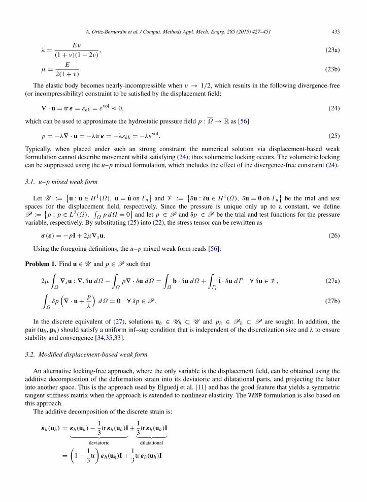
The elastic body becomes nearly-incompressible when ν → 1/2, which results in the following divergence-free(or incompressibility) constraint to be satisfied by the displacement field:

∇ · u = tr ε = εkk = εvol≈ 0, (24)

which can be used to approximate the hydrostatic pressure field p : Ω → R as [56]

p = −λ∇ · u = −λtr ε = −λεkk = −λεvol. (25)

Typically, when placed under such an strong constraint the numerical solution via displacement-based weakformulation cannot describe movement whilst satisfying (24); thus volumetric locking occurs. The volumetric lockingcan be suppressed using the u–p mixed formulation, which includes the effect of the divergence-free constraint (24).

3.1. u–p mixed weak form

Let U :=u : u ∈ H1(Ω), u = u on Γu

and V :=

δu : δu ∈ H1(Ω), δu = 0 on Γu

be the trial and test

spaces for the displacement field, respectively. Since the pressure is unique only up to a constant, we defineP :=

p : p ∈ L2(Ω),

Ω p dΩ = 0

and let p ∈ P and δp ∈ P be the trial and test functions for the pressure

variable, respectively. By substituting (25) into (22), the stress tensor can be rewritten as

σ (ε) = −pI + 2µ∇su. (26)

Using the foregoing definitions, the u–p mixed weak form reads [56]:

Problem 1. Find u ∈ U and p ∈ P such that

2µΩ

∇su : ∇sδu dΩ −

Ω

p∇ · δu dΩ =

Ω

b · δu dΩ +

Γt

t · δu dΓ ∀ δu ∈ V , (27a)Ωδp∇ · u +

p

λ

dΩ = 0 ∀ δp ∈ P. (27b)

In the discrete equivalent of (27), solutions uh ∈ Uh ⊂ U and ph ∈ Ph ⊂ P are sought. In addition, thepair (uh,ph) should satisfy a uniform inf–sup condition that is independent of the discretization size and λ to ensurestability and convergence [34,35,33].

3.2. Modified displacement-based weak form

An alternative locking-free approach, where the only variable is the displacement field, can be obtained using theadditive decomposition of the deformation strain into its deviatoric and dilatational parts, and projecting the latterinto another space. This is the approach used by Elguedj et al. [11] and has the good feature that yields a symmetrictangent stiffness matrix when the approach is extended to nonlinear elasticity. The VANP formulation is also based onthis approach.

The additive decomposition of the discrete strain is:

εh(uh) = εh(uh)−13

tr εh(uh)I deviatoric

+13

tr εh(uh)I dilatational

=

1 −

13

tr

εh(uh)I +13

tr εh(uh)I


=

1 −

13

tr

εh(uh)I +13εvol

h (uh)I

= εdevh (uh)+ εdil

h (uh), (28)

which is used to define a discrete modified strain denoted by εh(uh), where the bar indicates the application of aprojection operator πh on its unmodified dilatational part, i.e.

εh(uh) = εdevh (uh)+ πh

εdil

h (uh)

= εdevh (uh)+ εdil

h (uh). (29)

The projection operator in (29) has not been applied to the deviatoric part since the dilatational part is the responsiblefor the volumetric locking. The modified dilatational strain is to be understood as an improved strain that precludesvolumetric locking. A modified potential energy functional will be defined using (29).

Problem 2. The displacement uh ∈ Uh ⊂ U can be found as the unique minimum point of the modified potentialenergy functional Π :

Π (uh) = infuh

Ωψ[εh(uh)] dΩ −

Ω

b · uh dΩ −

Γt

t · uh dΓ . (30)

On taking the first variation of the modified functional leads to the following general modified discrete weak form:

Problem 3. Find the displacement uh ∈ Uh ⊂ U such thatΩ

σ h(εh(uh)) : εh(δuh) dΩ =Ω b · δuh dΩ +

Γt

t · δuh dΓ ∀ δuh ∈ Vh ⊂ V . (31)

By means of (22) and (28), the modified stress in (31) becomes:

σ h = 2µεh + λεvolh I. (32)

By substituting (29) and (32) into (31) yields the following modified discrete weak form for nearly-incompressiblelinear elastostatics:

Problem 4. Find the displacement uh ∈ Uh ⊂ U such thatΩ

2µεh(uh)+ λεvol

h (uh)I

:

1 −

13

tr

εh(δuh)I +13εvol

h (δuh)I

dΩ

=

Ω

b · δuh dΩ +

Γt

t · δuh dΓ ∀ δuh ∈ Vh ⊂ V . (33)

The final step is the construction of an appropriate operator πh that defines the ‘barred’ quantities in (33) suchthat volumetric locking is alleviated. In brief, the idea is to find such an operator from the pressure constraint (27b).This adopts the form of an L2 projection. To this end, (27b) can be rearranged and later solved for ph to arrive at thefollowing expression:

ph = −λπh(∇ · uh) = −λπh(tr εh(uh))

= −λtrπh(εh(uh)) = −λtr εh(uh) = −λεvolh (uh). (34)

If an expression like (34) is available, the pressure can be eliminated from the formulation making the systemuniquely determined by the displacement field; furthermore, the space Ph becomes a function of the space Uh ,namely Ph(Uh).


Fig. 1. Schematic representation of a two-dimensional simplicial tessellation for the VANP method.

3.3. Volume-averaged nodal projection operator

The explicit form of the projection operator is derived from the volume-averaged nodal pressure techniqueintroduced in the work of Ortiz et al. [26]. To this end, let the domain tessellation with simplices be denoted byT (Ω). The tessellation consists of 3-node triangular or 4-node tetrahedral cells denoted by C. The vertices of thetessellation, denoted by V(T ), are then used to define the standard node set N s . In addition to the standard node set,we define a barycenter node set as N b with nodes located at the barycenter of each cell C in the tessellation T (Ω). So,an enhanced node set is defined as N +

= N s∪ N b. Fig. 1 depicts a schematic representation of a two-dimensional

simplicial tessellation used in the VANP method.In our approach, the simplicial tessellation T (Ω) that connects the standard node set N s is generated using a

meshing software and the Gauss points locations are computed based on this mesh. The enhanced node set N + isconstructed when needed by adding the extra required nodes to the standard node set N s . This poses no problem oradditional complexity in the method since the flexibility of meshfree methods permits the addition of nodes to thesimplicial mesh very easily.

To obtain the projection operator, the pressure constraint (27b) is discretized using

ph(x) =

nb=1

φb(x)pb, (35a)

δph(x) =

nc=1

φc(x)δpc, (35b)

where n is the number of nodes in the node set N s , whose associated meshfree basis functions φi (i = b, c) have anonzero discrete value at the sampling point of Cartesian coordinate x. If Gauss integration is used, the coordinatesof the sampling point are the Cartesian coordinates of a given Gauss point. By substituting (35) into the pressureconstraint (27b), it can be shown that after relying on the arbitrariness of nodal pressure test functions and performingrow-sum on the discrete pressure term leads to the following volume-averaged nodal pressure [26]:

pc = −λ

Ωcφc(x)∇ · uh dΩΩcφc(x) dΩ

= −λ

Ωcφc(x)εvol

h dΩΩcφc(x) dΩ

, (36)

where the integration volume Ω has been replaced with Ωc to indicate that due to the row-sum procedure theintegration volume is the union of cells that are attached to node c associated with the pressure degree of freedom pc(see Fig. 2). Eq. (36) gives rise to the VANP operator as

πc[·] =

Ωcφc(x)[·] dΩ

Ωcφc(x) dΩ

. (37)


Fig. 2. Schematic representation of an integration volume for the computation of the VANP operator associated with node c.

As can be inferred from (36), the nodal operator applied to εvolh gives its nodal representation as

εvolc = πc[ε

volh ] =

Ωcφc(x)[εvol

h ] dΩΩcφc(x) dΩ

. (38)

Finally, by the linear combination ph =

c φc pc, the bar operator is given by the following projection operator:

π [·] =

nc=1

φc(x)πc[·] =

nc=1

φc(x)

Ωcφc(x)[·] dΩ

Ωcφc(x) dΩ

. (39)

Thus, εvolh is computed as follows:

εvolh = π [εvol

h ] =

nc=1

φc(x)πc[εvolh ] =

nc=1

φc(x)

Ωcφc(x)εvol

h dΩΩcφc(x) dΩ

=

nc=1

φc(x)εvolc . (40)

Because the VANP method has its roots in the u–p mixed formulation, it is important to consider the inf–supstability [33–35]. However, inf–sup stability is difficult to prove in meshfree methods. Therefore, we do not providean analytical proof for the inf–sup condition, but rather we mimic well-known inf–sup stable finite element schemes.To this end, first-order meshfree basis functions are used to construct the space Uh with the enhanced node set N +

and the space Ph(Uh) with the standard node set N s . This mimics the inf–sup stable MINI finite element [46]. Forhigh-order approximations, two inf–sup stable finite elements are considered: the second-order conforming Crouzeixand Raviart element [57] and the Taylor–Hood element [58]. The former is mimicked using second-order meshfreebasis functions to construct the space Uh with the enhanced node set N + and first-order meshfree basis functions toconstruct the space Ph(Uh)with the standard node set N s . The Taylor–Hood element is mimicked using second-ordermeshfree basis functions to construct the space Uh and first-order meshfree basis to construct the space Ph(Uh) bothwith the standard node set N s . It is stressed that this is done only for stability purposes. Ultimately, it is our interestto compare the VANP approach with the MINI element because both use the same tessellation.

For implementation purposes of the VANP operator, it should be noted that the use of the aforementioned meshfreediscretizations for construction of Uh and Ph(Uh) spaces imply that the basis functions that appear in the operator(39) are computed using the standard node set N s , but εvol

h in (40) using either the enhanced node set N + or thestandard node set N s depending on whether bubble enrichment is used or not, respectively, since εvol

h is computedfrom the displacement field.

3.4. Discrete equations

The discrete modified weak form is obtained by introducing the following approximations into (33):


uh(x) =

na=1

φa(x)ua, (41a)

δuh(x) =

nb=1

φb(x)δub, (41b)

where φa(x) and φb(x) are meshfree basis functions. Thus, the corresponding discrete strains that appear in themodified weak form (33) (in Voigt notation) become

εh(uh) =

na=1

Ba(x)ua, (42)

εh(δuh) =

nb=1

Bb(x)δub, (43)

εvolh (uh) =

nc=1

φc(x)πc

mT

na=1

Ba

ua, (44)

εvolh (δuh) =

nc=1

φc(x)πc

mT

nb=1

Bb

δub, (45)

where in two dimensions

m =1 1 0

T, (46)

Ba =

φa,x 00 φa,yφa,y φa,x

, (47)

and in three dimensions

m =1 1 1 0 0 0

T, (48)

Ba =

φa,x 0 0

0 φa,y 00 0 φa,zφa,y φa,x 0φa,z 0 φa,x

0 φa,z φa,y

. (49)

Finally, on collecting all these discrete quantities and replacing them into the modified weak form (33), and appealingto the arbitrariness of nodal variations leads to the following system of equations:

K1+ K2

+ K3+ K4

u = f, (50a)

where u is the column vector of nodal coefficients and

K1ab =

Ω

BTa ITdevCµBb dΩ , (50b)

K2ab = λ

Ω

BTa ITdevm

nc=1

φcπc

mTBb

dΩ , (50c)

K3ab =

13

Ω

m

nc=1

φcπc

mTBa

T

CµBb dΩ , (50d)


K4ab =

λ

3

Ω

m

nc=1

φcπc

mTBa

T

mn

c=1

φcπc

mTBb

dΩ , (50e)

fa =

Ωφab dΩ +

Γt

φa t dΓ (50f)

with the following matrices due to the Voigt notation:

Idev = I −13

mmT (I is the identity matrix) , (50g)

and the material matrix being

Cµ =

2µ 0 00 2µ 00 0 µ

(50h)

in two dimensions, or

Cµ =

2µ 0 0 0 0 00 2µ 0 0 0 00 0 2µ 0 0 00 0 0 µ 0 00 0 0 0 µ 00 0 0 0 0 µ

(50i)

in three dimensions. Once the nodal coefficients are obtained from (50a), the nodal displacement at node i of Cartesiancoordinates xi is computed by evaluating (41a) at x = xi .

4. Numerical integration

The cell-based integration of discrete quantities that depend on basis functions derivatives introduces integrationerrors when standard Gauss integration is used. To alleviate these integration errors in the VANP method, a specialprocedure is performed to correct the values of the nodal basis functions derivatives at the Gauss points.

A strain correction technique that alleviates integration errors in meshfree methods, ensures patch test satisfactionto machine precision and converges optimally for first-order meshfree approximations, was developed in Ref. [26]. Inthe present paper, second-order max-ent basis functions and second-order RPIM basis functions are used. Particularly,the derivatives of the latter ones are much more complicated than the derivatives of the former ones. Thus, the first-order correction presented in Ref. [26] is not sufficiently accurate for integration of the weak form integrals. Asa remedy, the third-order variationally consistent accurate integration scheme presented in Ref. [43] is adopted tocorrect the nodal basis functions derivatives on triangular meshes and we extend this rule to tetrahedral meshes.

The third-order integration scheme needs an integration cell that is obtained from a simplicial tessellation. Fig. 3depicts a typical tessellation and a representative integration cell in two dimensions for this scheme; the enhancednode set N + is also shown to remark that the nodal basis functions derivatives are to be computed using the enhancednode set since they stem from the displacement field.

The third-order accurate integration scheme for correction of nodal basis functions derivatives follows. Forsimplicity, the derivations are given in detail only for two-dimensions. The Cartesian coordinate system is chosen,where for convenience x ≡ x1 and y ≡ x2. In addition, n j ( j = 1, 2) is the j th component of the unit outward normalto a cell edge in the Cartesian coordinate system.

For the cubic approximation basis

p(x) =1 x1 x2 x1x1 x1x2 x2x2 x1x1x1 x1x1x2 x1x2x2 x2x2x2

T, (51)

the corresponding stress field is quadratic. That is, the stress can be represented using a quadratic basis as

σi j = a0 + a1x1 + a2x2 + a3x1x1 + a4x1x2 + a5x2x2. (52)


Fig. 3. Geometric entities for the third-order accurate integration scheme. (a) Simplicial tessellation, where the shaded region represents anintegration cell whose domain is denoted by Ωe and its boundary by ∂Ωe

= ∂Ωe1∂Ωe

2∂Ωe

3 ; and (b) the integration cell and nodes, where theinterior Gauss points are depicted as + and the boundary Gauss points as ∗. Note that depending on the support size of the nodal basis functions,nodes that are beyond the cell can contribute at a Gauss point if their basis functions take a nonzero value at that point.

Hence, the quadratic basis is

f (x) =1 x1 x2 x1x1 x1x2 x2x2

T, (53)

whose derivative (δi j is the Kronecker delta symbol) is

f, j (x) =0 δ1 j δ2 j 2x1δ1 j x2δ1 j + x1δ2 j 2x2δ2 j

T. (54)

The corrected nodal derivatives (see Eq. (35) in Ref. [43]) can be expressed asΩ eφa, j f (x) dΩ e

=

Γ eφa f (x)n j dΓ e

−

Ω eφa f, j (x) dΩ e, (55)

leading to the following integration constraints that are to be met by the meshfree basis functions derivatives:Ω eφa,1 dΩ e

=

Γ eφan1 dΓ e, (56a)

Ω eφa,1x1 dΩ e

=

Γ eφa x1n1 dΓ e

−

Ω eφa dΩ e, (56b)

Ω eφa,1x2 dΩ e

=

Γ eφa x2n1 dΓ e, (56c)

Ω eφa,1x1x1 dΩ e

=

Γ eφa x1x1n1 dΓ e

−

Ω eφa2x1 dΩ e, (56d)

Ω eφa,1x1x2 dΩ e

=


−

Ω eφa x2 dΩ e, (56e)

Ω eφa,1x2x2 dΩ e

=

Γ eφa x2x2n1 dΓ e (56f)

for φa,1, andΩ eφa,2 dΩ e

=

Γ eφan2 dΓ e, (56g)

Ω eφa,2x1 dΩ e

=

Γ eφa x1n2 dΓ e, (56h)

440 A. Ortiz-Bernardin et al. / Comput. Methods Appl. Mech. Engrg. 285 (2015) 427–451Ω eφa,2x2 dΩ e

=

Γ eφa x2n2 dΓ e

−

Ω eφa dΩ e, (56i)

Ω eφa,2x1x1 dΩ e

=

Γ eφa x1x1n2 dΓ e, (56j)

Ω eφa,2x1x2 dΩ e

=


−

Ω eφa x1 dΩ e, (56k)

Ω eφa,2x2x2 dΩ e

=


−

Ω eφa2x2 dΩ e (56l)

for φa,2.The integration constraints (56) are solved using Gauss integration on the integration cell shown in Fig. 3(b), which

leads to the following system of linear equations:

Qd j = f j , j = 1, 2 (57a)

where Q and f j are given in Ref. [43] (see Eq. (42) therein), and the j th corrected basis function derivative at the sixinterior Gauss points of coordinates xi (i = 1, 2, . . . , 6) is given by the solution vector

d j =φa, j (x1) φa, j (x2) φa, j (x3) φa, j (x4) φa, j (x5) φa, j (x6)

T. (57b)

In the preceding equations, the index a runs through the combined nodal contribution3 that results from the union ofnodal contributions corresponding to each of the interior and edge Gauss points in the cell.

The corrected derivatives given in (57b) are used to define the deformation matrix (Eq. (47) or (49)) that appearsin the stiffness matrices of the VANP method.

Finally, in three dimensions the integration cell is a tetrahedron and the integration constraints can be derived fromthe quadratic basis

f (x) =1 x1 x2 x3 x1x1 x2x2 x3x3 x1x2 x1x3 x2x3

T, (58)

and its derivative

f, j (x) =0 δ1 j δ2 j δ3 j 2x1δ1 j 2x2δ2 j 2x3δ3 j x2δ1 j + x1δ2 j x3δ1 j + x1δ3 j x3δ2 j + x2δ3 j

T. (59)

The third-order integration scheme has not been developed for tetrahedral cells in Ref. [43]. Therefore, thequadratures that are needed for tetrahedral cells are given in the Appendix.

5. Numerical examples

In this section, the performance and accuracy of the VANP formulation are assessed via numerical examples. Thefollowing notation is adopted for presenting the VANP results: VANP-T a

p /Tq -b, where Tp is the approximation spaceof polynomial order p for the displacement field and Tq is the approximation space of polynomial order q in which thedilatational strain is projected; the superscript a is set as follows: a = + when bubble enrichment is specified (N + isthe node set used) or it is removed in case bubble enrichment is not considered (N s is the node set used); and b standsfor the type of meshfree basis function that is used for the approximation spaces. Thus, b = m is used for max-entbasis functions, whereas b = r for RPIM basis functions. By using the preceding definitions the following VANPschemes are considered: VANP-T +

1 /T1-m, VANP-T +

2 /T1-m, VANP-T +

2 /T1-r, VANP-T2/T1-m, VANP-T2/T1-r.In all the VANP computations, the third-order variationally consistent accurate integration scheme detailed in

Section 4 is used and the nodal pressure is obtained from the computed nodal coefficients using (36). The basebackground mesh, which only contains the node set N s , is generated using a meshing software. The enhanced nodeset N + is constructed when needed by adding the extra required nodes to the standard node set N s .

3 The nodal contribution at a given Gauss point of coordinate x is defined as the indices of the nodes whose basis functions have a nonzero valueat x.


Fig. 4. Cantilever beam problem. Model geometry and boundary conditions.

5.1. Cantilever beam

To show the accuracy and convergence of the VANP method in nearly-incompressible elasticity, a cantilever beamof unit thickness with a parabolic end load P is considered. Fig. 4 presents the geometry of the beam. A regularbackground mesh of 3-node triangles with a mesh pattern of 2n divisions along the length of the beam and n divisionsalong the height of the beam is chosen for the definition of node set N s . The coarsest mesh is obtained with n = 4.The essential boundary conditions on the clamped edge are applied according to the analytical solution given byTimoshenko and Goodier [59]:

ux = −Py

6E I

(6L − 3x)x + (2 + ν)y2

−3D2

2(1 + ν)

, (60a)

u y =P

6E I

3νy2(L − x)+ (3L − x)x2

, (60b)

where E = E/1 − ν2

with the Young’s modulus set to E = 210 000 MPa and ν = ν/ (1 − ν) with the Poisson’s

ratio set to ν = 0.4999; L = 200 mm is the length of the beam, D = 100 mm is the height of the beam, and I thesecond-area moment of the beam section. The total load on the traction boundary is P = −5000 N.

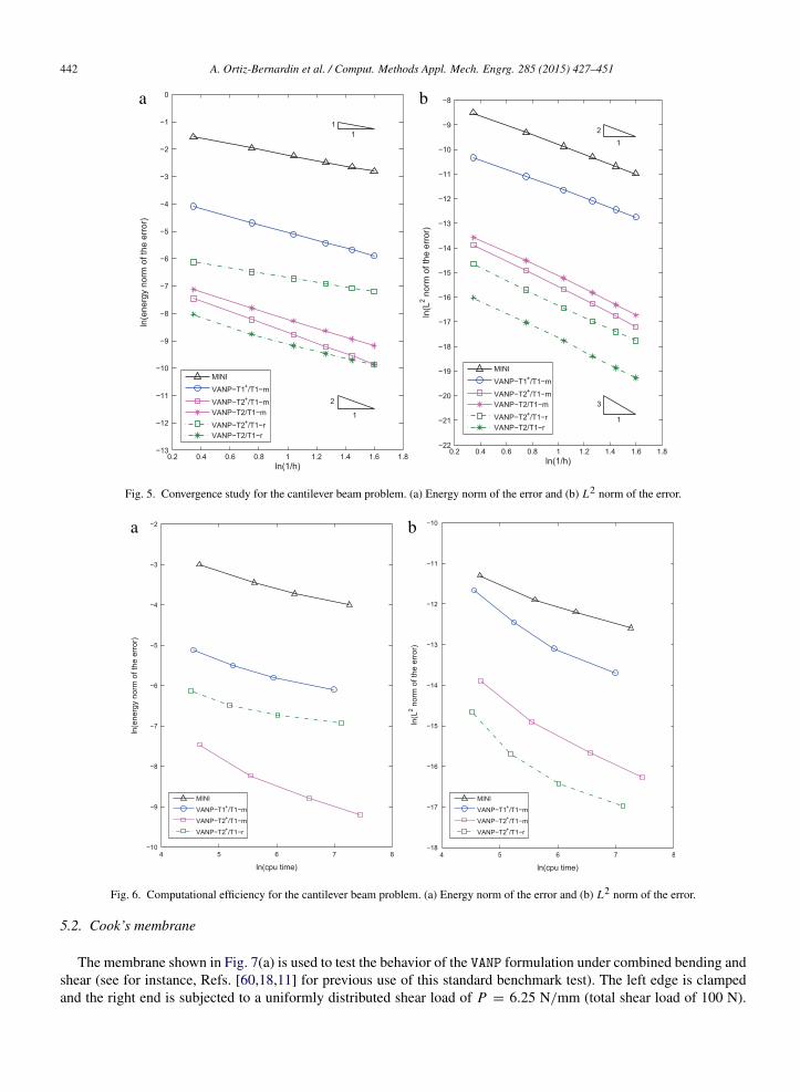
The convergence rates in the energy and L2 norms of the error are depicted in Fig. 5. In the convergence plots, thenodal spacing is set to the length of the element side and denoted by h. The convergence rates in the energy normof the error are presented in Fig. 5(a). The optimal convergence rates in the energy norm of the error are 1 for lineardisplacements and 2 for quadratic displacements [56]. From Fig. 5(a), it is observed that both the MINI element andVANP-T +

1 /T1-m schemes deliver the optimal rate of convergence, but the latter is more accurate than the former.With respect to the second-order maxent approaches, the VANP-T +

2 /T1-m scheme delivers the optimal convergencerate, whereas the VANP-T2/T1-m slightly loses the optimal convergence due to the absence of bubble enrichment. Onthe other hand, the second-order RPIM schemes, VANP-T +

2 /T1-r and VANP-T2/T1-r, only exhibit linear convergence.The convergence rates in the L2-norm of the error are shown in Fig. 5(b). The optimal convergence rates in the

L2-norm of the error are 2 for linear displacements and 3 for quadratic displacements [56]. Once again, both the MINIelement and the VANP-T +

1 /T1-m schemes deliver the optimal rate of convergence, but the latter is more accurate thanthe former; all the second-order VANP approaches exhibit the optimal rate of convergence in the L2-norm of the error.

Finally, the computational efficiency of the different approaches is studied. In order to compare the first withsecond order methods, the energy and L2 norms of the errors of the first order methods were computed with morerefined meshes to obtain accuracies comparable to the accuracies of the second order methods; and to compare theVANP formulation with the MINI element, only the bubble-enriched VANP methods are considered. The computationalefficiency of the different approaches is presented in Fig. 6. All the VANP methods are more efficient than the MINIelement in both the energy and L2 norms of the error when a certain level of accuracy is desired, particularly, as themesh is refined.


Fig. 5. Convergence study for the cantilever beam problem. (a) Energy norm of the error and (b) L2 norm of the error.

Fig. 6. Computational efficiency for the cantilever beam problem. (a) Energy norm of the error and (b) L2 norm of the error.

5.2. Cook’s membrane

The membrane shown in Fig. 7(a) is used to test the behavior of the VANP formulation under combined bending andshear (see for instance, Refs. [60,18,11] for previous use of this standard benchmark test). The left edge is clampedand the right end is subjected to a uniformly distributed shear load of P = 6.25 N/mm (total shear load of 100 N).


Fig. 7. Cook’s membrane problem. (a) Model geometry and boundary conditions; (b) sample regular background mesh; and (c) unstructuredbackground mesh.

Fig. 8. Cook’s membrane problem. Convergence of the vertical tip displacement.

The following material parameters are set: E = 240.565 MPa and ν = 0.4999. A regular background mesh of 3-nodetriangles with a mesh pattern of n × n divisions per side is chosen for the definition of node set N s . A reference meshfor n = 20 is shown in Fig. 7(b). The unstructured background mesh depicted in Fig. 7(c) is also considered for sometests.

A first study is devoted to the convergence of the vertical tip displacement at point A upon mesh refinement. Theresults are summarized in Fig. 8. The numerical results reveal that the VANP approaches deliver better convergencethan the MINI element and that VANP-T +

1 /T1-m and VANP-T +

2 /T1-r are in good agreement between them and bothconverge to the reference value (around 8 mm) obtained from Ref. [11]. The scheme without bubbles VANP-T2/T1-ralso exhibits good convergence to the reference value, although slightly inferior to the convergence of the former VANPcases.

A second study is performed to show the smoothness of the nodal pressure delivered by the VANP formulation. Here,the nodal pressure is measured along the line BC (see Fig. 7(a)) using the structured mesh shown in Fig. 7(b). Theresults are depicted in Fig. 9. It is observed that the MINI element exhibits small pressure oscillations near the startingand ending points on the line BC, whereas the VANP-T +

1 /T1-m scheme delivers smooth pressure along the wholeline. The VANP-T +

2 /T1-r approach also delivers smooth pressure along the whole line. However, the VANP-T2/T1-r


Fig. 9. Cook’s membrane problem. Nodal pressure along the line BC .

scheme, which has no bubble enrichment, presents severe pressure oscillations. Finally, the nodal pressure is computedusing the unstructured mesh depicted in Fig. 7(c). The pressure smoothness delivered by the VANP formulation isreadily evident in the pictorial shown in Fig. 10, where only the VANP-T2/T1-r scheme exhibits pressure oscillationsdue to the absence of bubble enrichment.

5.3. Plane strain compression of a constrained block

This compression problem is used to evaluate the VANP formulation in a highly constrained setting in twodimensions. Similar benchmark problems are found in Refs. [18,61,62]. As shown in Fig. 11(a), a square block ofdimensions 1 × 1 mm and unit thickness is fully constrained on its Dirichlet boundary (bottom, left, and right edges).A downward traction of 4000 N/mm is applied over the center portion of the top edge covering 1/3 of the edge’slength. The following material parameters are specified: E = 210 000 MPa and ν = 0.4999. Plane strain condition isassumed. A reference background mesh of 3-node triangles for the definition of the node set N s is shown in Fig. 11(b)for a regular tessellation and in Fig. 11(c) for an unstructured one. In this example, the non-bubble-enriched schemesare not shown since they produce highly oscillatory pressure fields and therefore are not stable. This lack of stabilityhas already been demonstrated in the previous examples.

The compression level is defined as the ratio of the absolute value of the vertical displacement at point A to theheight of the block. In the first test, the convergence of the compression level upon mesh refinement of the regularmesh is studied. The results for the MINI element and first- and second-order VANP schemes are presented in Fig. 12.All the schemes show convergence as the mesh is refined. However, the MINI element scheme presents a slowerconvergence.

The second test is devoted to study the smoothness of the nodal pressure variable. For this purpose the unstructuredmesh shown in Fig. 11(c) is considered. The nodal pressures are shown in Fig. 13. It is observed that the nodal pressureis reasonable smooth for the MINI element formulation (Fig. 13(a)); however, the first-order max-ent VANP schemepresents even smoother pressure fields (Fig. 13(b)). Smooth pressure is also obtained for the second-order enrichedVANP schemes (Fig. 13(c) and (d)).

5.4. Compression of a constrained block

Finally, a three-dimensional highly constrained problem is considered. A rectangular block of dimensions1 × 0.5 × 0.5 mm is constrained as shown in Fig. 14(a). The downward traction is 1000 MPa. The following materialparameters are set: E = 210 000 MPa and ν = 0.4999. For the construction of the node set N s , the faces of therectangular domain are divided as follows: 2n divisions along the length, n divisions along the height, and n divisions


Fig. 10. Cook’s membrane problem. Nodal pressure variable on the unstructured background mesh for (a) MINI element, (b) VANP-T +

1 /T1-m,

(c) VANP-T +

2 /T1-r, and (d) VANP-T2/T1-r.

along the depth. A regular background mesh of 4-node tetrahedra is generated to define the node set N s . A samplemesh for n = 6 is shown in Fig. 14(b).

The compression level is defined as the ratio of the absolute value of the vertical displacement on edge AB to theheight of the block. The convergence of the compression level upon mesh refinement is presented in Fig. 15. In thisparticular example, the MINI element converges and performs as good as the max-ent VANP schemes. Although theVANP-T +

2 /T1-r scheme shows a tendency to converge, it does it significantly slower than the rest of the schemes.With respect to the smoothness of the nodal pressure variable, Fig. 16 reveals that the MINI element presents small

pressure oscillations. In contrast, the VANP-T +

1 /T1-m and VANP-T +

2 /T1-m schemes present smooth pressure fields.On the other hand, the pressure field for the VANP-T +

2 /T1-r scheme behaves oscillatory.


Fig. 11. Plane strain compression of a constrained block. (a) Model geometry and boundary conditions; (b) sample regular background mesh; and(c) unstructured background mesh.

Fig. 12. Plane strain compression of a constrained block. Convergence of the compression level at point A.

6. Conclusions

In this paper, a high-order displacement-based Galerkin meshfree method has been proposed for the analysisof nearly-incompressible linear elastic solids using the nodal information from low-order triangular/tetrahedraltessellations. In this procedure, a projection operator is constructed from the pressure constraint of the u–p mixedformulation and used to project the dilatational strain onto an approximation space of equal- or lower-order than theapproximation space for the displacement field. The stability of the method is provided via bubble-like functions,which requires the addition of an interior node to every cell in the simplicial tessellation. This, however, is a straight-forward task due to the flexibility offered by meshfree methods. First and second order both max-ent and RPIMbasis functions were considered as particular cases to exemplify the VANP formulation. The low-order tessellation isalso used to numerically integrate the VANP weak form integrals. For accuracy purposes, the third-order variationallyconsistent accurate integration rule of Duan et al. [43] was adopted for triangular meshes and an extension of this ruleto three dimensions was developed for integration on tetrahedral meshes.

The performance of the VANP formulation was assessed through several examples in two and three dimensions. Theresults showed that the method is devoid of volumetric locking and that the enrichment of the displacement field withbubble-like nodes is fundamental to obtain smooth nodal pressures from the computed displacement field. The rates


Fig. 13. Plane strain compression of a constrained block. Nodal pressure variable for (a) MINI element, (b) VANP-T +

1 /T1-m, (c) VANP-T +

2 /T1-m,

and (d) VANP-T +

2 /T1-r. In these plots the unstructured background mesh depicted in Fig. 11(c) is used.

Fig. 14. Compression of a constrained block. (a) Model geometry and boundary conditions, and (b) sample background mesh.

of convergence in the energy and L2-norm of the error were found to be optimal in first and second order max-entVANP schemes, whereas second-order RPIM VANP schemes converged optimally in the L2-norm and only linearlyin the energy norm. In comparing the VANP approach with its finite element counterpart, the MINI element [46], itcan be stated that the VANP approach provides greater efficiency, greater accuracy and better convergence propertieson low-order simplicial tessellations. An extension of the VANP formulation to nonlinear regime is currently underinvestigation.


Fig. 15. Compression of a constrained block. Convergence of the compression level on edge AB.

Fig. 16. Compression of a constrained block. Nodal pressure variable for (a) MINI element, (b) VANP-T +

1 /T1-m, (c) VANP-T +

2 /T1-m, and

(d) VANP-T +

2 /T1-r.

Acknowledgments

A. Ortiz-Bernardin would like to express his gratitude for the financial support provided by CONICYT-FONDECYT/Iniciacion under Grant No. 11110389. J. S. Hale and C. J. Cyron acknowledge the funding providedby CONICYT-FONDECYT/Iniciacion under Grant No. 11110389, which made possible a short research stay inChile. The work of Jack S. Hale is supported by the National Research Fund, Luxembourg (Grant No. 6693582), andcofunded under the Marie Carie Actions of the European Commission (FP7-COFUND).


Appendix. Quadratures for the tetrahedral cell

The quadratures given here ensure invertibility of Q in (57). For a tetrahedral cell, the following 10-point rule isused for the interior Gauss points:

T =

0.7784952948213300 0.0738349017262234 0.0738349017262234 0.07383490172622340.0738349017262234 0.7784952948213300 0.0738349017262234 0.07383490172622340.0738349017262234 0.0738349017262234 0.7784952948213300 0.07383490172622340.0738349017262234 0.0738349017262234 0.0738349017262234 0.77849529482133000.4062443438840510 0.4062443438840510 0.0937556561159491 0.09375565611594910.4062443438840510 0.0937556561159491 0.4062443438840510 0.09375565611594910.4062443438840510 0.0937556561159491 0.0937556561159491 0.40624434388405100.0937556561159491 0.4062443438840510 0.4062443438840510 0.09375565611594910.0937556561159491 0.4062443438840510 0.0937556561159491 0.40624434388405100.0937556561159491 0.0937556561159491 0.4062443438840510 0.4062443438840510

(A.1)

as the tetrahedral coordinates, and

w =

0.04763313484320890.04763313484320890.04763313484320890.04763313484320890.13491124343786100.13491124343786100.13491124343786100.13491124343786100.13491124343786100.1349112434378610

(A.2)

as the corresponding weights; whereas the following 6-point rule is used for the face Gauss points of the tetrahedralcell:

T =

0.816847572980459 0.091576213509771 0.0915762135097710.091576213509771 0.816847572980459 0.0915762135097710.091576213509771 0.091576213509771 0.8168475729804590.108103018168070 0.445948490915965 0.4459484909159650.445948490915965 0.108103018168070 0.4459484909159650.445948490915965 0.445948490915965 0.108103018168070

(A.3)

as the triangular coordinates, and

w =

0.1099517436553220.1099517436553220.1099517436553220.2233815896780110.2233815896780110.223381589678011

(A.4)

as the corresponding weights.

References

[1] J.C. Simo, R.L. Taylor, K.S. Pister, Variational and projection methods for the volume constraint in finite deformation elasto-plasticity,Comput. Methods Appl. Mech. Engrg. 51 (1–3) (1985) 177–208.

[2] J.C. Simo, F. Armero, Geometrically non-linear enhanced strain mixed methods and the method of incompatible modes, Internat. J. Numer.Methods Engrg. 33 (7) (1992) 1413–1449.

http://refhub.elsevier.com/S0045-7825(14)00444-7/sbref1



[3] T. Sussman, K.J. Bathe, A finite element formulation for nonlinear incompressible elastic and inelastic analysis, Comput. Struct. 26 (1–2)(1987) 357–409.

[4] P. Hansbo, M.G. Larson, Discontinuous Galerkin methods for incompressible and nearly incompressible elasticity by Nitsche’s method,Comput. Methods Appl. Mech. Engrg. 191 (17–18) (2002) 1895–1908.

[5] T.P. Wihler, Locking-free DGFEM for elasticity problems in polygons, IMA J. Numer. Anal. 24 (1) (2004) 45–75.[6] R. Liu, M.F. Wheeler, C.N. Dawson, A three-dimensional nodal-based implementation of a family of discontinuous Galerkin methods for

elasticity problems, Comput. Struct. 87 (3–4) (2009) 141–150.[7] R. Falk, Nonconforming finite element methods for the equations of linear elasticity, Math. Comp. 57 (196) (1991) 529–550.[8] L.-H. Wang, H. Qi, A locking-free scheme of nonconforming rectangular finite element for the planar elasticity, J. Comput. Math. 22 (5)

(2004) 641–650.[9] S. Chen, G. Ren, S. Mao, Second-order locking-free nonconforming elements for planar linear elasticity, J. Comput. Appl. Math. 233 (10)

(2010) 2534–2548.[10] T.J.R. Hughes, Generalization of selective integration procedures to anisotropic and nonlinear media, Internat. J. Numer. Methods Engrg. 15

(9) (1980) 1413–1418.[11] T. Elguedj, Y. Bazilevs, V. Calo, T.J.R. Hughes, B-bar and F-bar projection methods for nearly incompressible linear and non-linear elasticity

and plasticity using higher-order NURBS elements, Comput. Methods Appl. Mech. Engrg. 1 (33–40) (2008) 2667–3172.[12] F. Auricchio, L. Beirao da Veiga, C. Lovadina, A. Reali, An analysis of some mixed-enhanced finite element for plane linear elasticity,

Comput. Methods Appl. Mech. Engrg. 194 (27–29) (2005) 2947–2968.[13] C. Lovadina, F. Auricchio, On the enhanced strain technique for elasticity problems, Comput. Struct. 81 (8–11) (2003) 777–787.[14] R.L. Taylor, A mixed-enhanced formulation for tetrahedral finite elements, Internat. J. Numer. Methods Engrg. 47 (1–3) (2000) 205–227.[15] E. Onate, J. Rojek, R.L. Taylor, O.C. Zienkiewicz, Finite calculus formulation for incompressible solids using linear triangles and tetrahedra,

Internat. J. Numer. Methods Engrg. 59 (11) (2004) 1473–1500.[16] M. Cervera, M. Chiumenti, Q. Valverde, C. Agelet de Saracibar, Mixed linear/linear simplicial elements for incompressible elasticity and

plasticity, Comput. Methods Appl. Mech. Engrg. 192 (49–50) (2003) 5249–5263.[17] O.C. Zienkiewicz, J. Rojek, R.L. Taylor, M. Pastor, Triangles and tetrahedra in explicit dynamic codes for solids, Internat. J. Numer. Methods

Engrg. 43 (3) (1998) 565–583.[18] E.A. de Souza Neto, F.M.A. Pires, D.R.J. Owen, F-bar-based linear triangles and tetrahedra for finite strain analysis of nearly incompressible

solids. Part I: formulation and benchmarking, Internat. J. Numer. Methods Engrg. 62 (3) (2005) 353–383.[19] P. Thoutireddy, J.F. Molinari, E.A. Repetto, M. Ortiz, Tetrahedral composite finite elements, Internat. J. Numer. Methods Engrg. 53 (6) (2002)

1337–1351.[20] Y. Guo, M. Ortiz, T. Belytschko, E.A. Repetto, Triangular composite finite elements, Internat. J. Numer. Methods Engrg. 47 (1–3) (2000)

287–316.[21] J. Bonet, A.J. Burton, A simple average nodal pressure tetrahedral element for incompressible and nearly incompressible dynamic explicit

applications, Comm. Numer. Methods Engrg. 14 (5) (1998) 437–449.[22] C.R. Dohrmann, M.W. Heinstein, J. Jung, S.W. Key, W.R. Witkowski, Node-based uniform strain elements for three-node triangular and

four-node tetrahedral meshes, Internat. J. Numer. Methods Engrg. 47 (9) (2000) 1549–1568.[23] J. Bonet, M. Marriot, O. Hassan, An averaged nodal deformation gradient linear tetrahedral element for large strain explicit dynamic

applications, Comm. Numer. Methods Engrg. 17 (8) (2001) 551–561.[24] M.A. Puso, J. Solberg, A stabilized nodally integrated tetrahedral, Internat. J. Numer. Methods Engrg. 67 (6) (2006) 841–867.[25] M. Broccardo, M. Micheloni, P. Krysl, Assumed-deformation gradient finite elements with nodal integration for nearly incompressible large

deformation analysis, Internat. J. Numer. Methods Engrg. 78 (9) (2009) 1113–1134.[26] A. Ortiz, M.A. Puso, N. Sukumar, Maximum-entropy meshfree method for compressible and near-incompressible elasticity, Comput. Methods

Appl. Mech. Engrg. 199 (25–28) (2010) 1859–1871.[27] B.P. Lamichhane, Inf-sup stable finite-element pairs based on dual meshes and bases for nearly incompressible elasticity, IMA J. Numer.

Anal. 29 (2) (2009) 404–420.[28] B.P. Lamichhane, From the Hu–Washizu formulation to the average nodal strain formulation, Comput. Methods Appl. Mech. Engrg. 198

(49–52) (2009) 3957–3961.[29] P. Krysl, B. Zhu, Locking-free continuum displacement finite elements with nodal integration, Internat. J. Numer. Methods Engrg. 76 (7)

(2008) 1020–1043.[30] G. Castellazzi, P. Krysl, Patch-averaged assumed strain finite elements for stress analysis, Internat. J. Numer. Methods Engrg. 90 (13) (2012)

1618–1635.[31] J.C. Simo, T.J.R. Hughes, On the variational foundations of assumed strain methods, J. Appl. Mech. 53 (1) (1986) 51–54.[32] H. Nguyen-Xuan, G.R. Liu, An edge-based smoothed finite element method softened with a bubble function (bES-FEM) for solid mechanics

problems, Comput. Struct. 128 (0) (2013) 14–30.[33] F. Brezzi, On the existence, uniqueness and approximation of saddle-point problems arising from Lagrangian multipliers, RAIRO Anal.

Numer. 8 (1974) 129–151.[34] O.A. Ladyzhenskaya, The Mathematical Theory of Viscous Incompressible Flows, 2nd English ed., Gordon and Breach, London, 1969.[35] I. Babuska, The finite element method with Lagrangian multipliers, Numer. Math. 20 (3) (1973) 179–192.[36] J. Dolbow, T. Belytschko, Numerical integration of Galerkin weak form in meshfree methods, Comput. Mech. 23 (3) (1999) 219–230.[37] I. Babuska, U. Banerjee, J.E. Osborn, Q.L. Li, Quadrature for meshless methods, Internat. J. Numer. Methods Engrg. 76 (9) (2008) 1434–1470.[38] I. Babuska, U. Banerjee, J.E. Osborn, Q. Zhang, Effect of numerical integration on meshless methods, Comput. Methods Appl. Mech. Engrg.

198 (37–40) (2009) 2886–2897.[39] J.S. Chen, C.T. Wu, S. Yoon, Y. You, A stabilized conforming nodal integration for Galerkin mesh-free methods, Internat. J. Numer. Methods

Engrg. 50 (2) (2001) 435–466.







































[40] A. Ortiz, M. Puso, N. Sukumar, Maximum-entropy meshfree method for incompressible media problems, Finite Elem. Anal. Des. 47 (6)(2011) 572–585.

[41] Q. Duan, X. Li, H. Zhang, T. Belytschko, Second-order accurate derivatives and integration schemes for meshfree methods, Internat. J. Numer.Methods Engrg. 92 (4) (2012) 399–424.

[42] J.-S. Chen, M. Hillman, M. Ruter, An arbitrary order variationally consistent integration for Galerkin meshfree methods, Internat. J. Numer.Methods Engrg. 95 (5) (2013) 387–418.

[43] Q. Duan, X. Gao, B. Wang, X. Li, H. Zhang, T. Belytschko, Y. Shao, Consistent element-free Galerkin method, Internat. J. Numer. MethodsEngrg. 99 (2) (2014) 79–101.

[44] Q. Duan, X. Gao, B. Wang, X. Li, H. Zhang, A four-point integration scheme with quadratic exactness for three-dimensional element-freeGalerkin method based on variationally consistent formulation, Comput. Methods Appl. Mech. Engrg. 280 (0) (2014) 84–116.

[45] C. Wu, W. Hu, Meshfree-enriched simplex elements with strain smoothing for the finite element analysis of compressible and nearlyincompressible solids, Comput. Methods Appl. Mech. Engrg. 200 (45–46) (2011) 2991–3010.

[46] D.N. Arnold, F. Brezzi, M. Fortin, A stable finite element for the Stokes equations, Calcolo 21 (4) (1984) 337–344.[47] N. Sukumar, Construction of polygonal interpolants: a maximum entropy approach, Internat. J. Numer. Methods Engrg. 61 (12) (2004)

2159–2181.[48] M. Arroyo, M. Ortiz, Local maximum-entropy approximation schemes: a seamless bridge between finite elements and meshfree methods,

Internat. J. Numer. Methods Engrg. 65 (13) (2006) 2167–2202.[49] N. Sukumar, R.W. Wright, Overview and construction of meshfree basis functions: from moving least squares to entropy approximants,

Internat. J. Numer. Methods Engrg. 70 (2) (2007) 181–205.[50] C.J. Cyron, M. Arroyo, M. Ortiz, Smooth, second order, non-negative meshfree approximants selected by maximum entropy, Internat. J.

Numer. Methods Engrg. 79 (13) (2009) 1605–1632.[51] J.G. Wang, G.R. Liu, A point interpolation meshless method based on radial basis functions, Internat. J. Numer. Methods Engrg. 54 (11)

(2002) 1623–1648.[52] G.R. Liu, Meshfree Methods: Moving Beyond the Finite Element Method, second ed., CRC Press, Boca Raton, FL, 2010.[53] F. Greco, N. Sukumar, Derivatives of maximum-entropy basis functions on the boundary: theory and computations, Internat. J. Numer.

Methods Engrg. 94 (12) (2013) 1123–1149.[54] G.E. Fasshauer, Meshfree Approximation Methods with MATLAB, World Scientific Pub. Co. Inc., 2007.[55] M.D. Buhmann, A new class of radial basis functions with compact support, Math. Comp. 70 (233) (2000) 307–318.[56] T.J.R. Hughes, The Finite Element Method: Linear Static and Dynamic Finite Element Analysis, Dover Publications, Inc., Mineola, NY,

2000.[57] M. Crouzeix, P.-A. Raviart, Conforming and nonconforming finite element methods for solving the stationary Stokes equations. I, Rev. Fr.

Autom. Inform. Rech. Oper. R7 (3) (1974) 33–76.[58] P. Hood, C. Taylor, Navier–Stokes equations using mixed interpolations, in: J.T. Oden, O.C. Zienkiewicz, R.H. Gallagher, C. Taylor (Eds.),

Finite Element Methods in Flow Problems, UAH Press, The University of Alabama in Huntsville, Huntsville, AL, 1974, pp. 121–132.[59] S.P. Timoshenko, J.N. Goodier, Theory of Elasticity, third ed., McGraw-Hill, NY, 1970.[60] J.C. Simo, S. Rifai, A class of mixed assumed strain methods and the method of incompatible modes, Internat. J. Numer. Methods Engrg. 29

(8) (1990) 1595–1638.[61] P. Hauret, E. Kuhl, M. Ortiz, Diamond elements: a finite element/discrete-mechanics approximation scheme with guaranteed optimal

convergence in incompressible elasticity, Internat. J. Numer. Methods Engrg. 72 (3) (2007) 253–294.[62] N. Kikuchi, Remarks on 4CST-elements for incompressible materials, Comput. Methods Appl. Mech. Engrg. 37 (1) (1983) 109–123.
























Documents

Volume-averaged nodal projection method for nearly ...mediatum.ub.tum.de/doc/1290404/315058.pdf · Volume-averaged nodal projection method for ... We present a displacement-based