Embed Size (px)
Citation preview
PHASE 2 REPORT - REVIEW COPY FURTHER SITE CHARACTERIZATION AND ANALYSIS
VOLUME 2C - DATA EVALUATION AND INTERPRETATION REPORT HUDSON RIVER PCBs REASSESSMENT RI/FS February 1997 For U.S. Environmental Protection Agency Region II and U.S. Army Corps of Engineers Kansas City District Volume 2C Book 1 of 3 TAMS CONSULTANTS, Inc. The CADMUS Group, Inc. Gradient Corporation

PHASE 2 REPORT - REVIEW COPY FURTHER SITE CHARACTERIZATION AND ANALYSIS
VOLUME 2C - DATA EVALUATION AND INTERPRETATION REPORT HUDSON RIVER PCBs REASSESSMENT RI/FS
TAMS/Cadmus/Gradient i
Table of Contents Page VOLUME 2C (BOOK 1 OF 3) TABLE OF CONTENTS ...................................................................................................................... i
LIST OF TABLES ...............................................................................................................v LIST OF FIGURES.......................................................................................................... viii LIST OF PLATES............................................................................................................. xv
EXECUTIVE SUMMARY ............................................................................................................... E-1 CHAPTER 1
INTRODUCTION.......................................................................................................... 1-1 1.1 Purpose of Report 1-1 1.2 Report Format and Organization........................................................................ 1-2 1.3 Technical Approach of the Data Evaluation and Interpretation Report . . . . . 1-2 1.4 Review of the Phase 2 Investigations ................................................................. 1-5
1.4.1 Review of PCB Sources.......................................................................... 1-5 1.4.2 Water Column Transport Investigation .................................................. 1-6 1.4.3 Assessment of Sediment PCB Inventory and Fate .................................. 1-9 1.4.4 Analytical Chemistry Program................................................................ 1-14
CHAPTER 2
PCB SOURCES TO THE UPPER AND LOWER HUDSON RIVER.......................... 2-1 2.1 Background ......................................................................................................... 2-1 2.2 Upper Hudson River Sources.............................................................................. 2-2
2.2.1 NYSDEC Registered Inactive Hazardous Waste Disposal Sites............ 2-2 2.2.2 Remnant Deposits ..........................................................................................2-18 2.2.3 Dredge Spoil Sites..........................................................................................2-21 2.2.4 Other Upper Hudson Sources ........................................................................2-22
2.3 Lower Hudson River Sources ........................................................................... 2-22 2.3.1 Review of Phase 1 Analysis........................................................................... 2-23 2.3.2 Sampling of Point Sources in New York/New Jersey (NY/NJ) Harbor 2-23 2.3.3 Other Downstream External Sources............................................................. 2-28
CHAPTER 3
WATER COLUMN PCB FATE AND TRANSPORT IN THE HUDSON RIVER ...... 3-1 3.1 PCB Equilibrium Partitioning.................................................................................... 3-3
3.1.1 Two-Phase Models of Equilibrium Partitioning ............................................ 3-4 3.1.2 Three-Phase Models of Equilibrium Partitioning .......................................... 3-23 3.1.3 Sediment Equilibrium Partition Coefficients.................................................3-31 3.1.4 Summary ................................................................................................ 3-38
3.2 Water Column Mass Loading ....................................................................................3-39
PHASE 2 REPORT - REVIEW COPY FURTHER SITE CHARACTERIZATION AND ANALYSIS
VOLUME 2C - DATA EVALUATION AND INTERPRETATION REPORT HUDSON RIVER PCBs REASSESSMENT RI/FS
Table of Contents (cont=d)
TAMS/Cadmus/Gradient ii
3.2.1 Phase 2 Water and Sediment Characterization ..............................................3-40 3.2.2 Flow Estimation .................................................................................... 3-41 3.2.3 Fate Mechanisms ........................................................................................... 3-45 3.2.4 Conceptual Model of PCB Transport in the Upper Hudson ............................ 3-57 3.2.5 River Characterization ................................................................................... 3-59 3.2.6 Mass Load Assessment .................................................................................. 3-67 3.2.7 Source Loading Quantitation ................................................................. 3-84
3.3 Historical Water Column Transport of PCBs ................................................... 3-88 3.3.1 Establishing Sediment Core Chronologies .................................................... 3-90 3.3.2 Surface Sediment Characterization ............................................................ 3-102 3.3.3 Water Column Transport of PCBs Shown by Sediment Deposited
After 1975 ......................................................................................................3-104 3.3.4 Estimation of the PCB Load and Concentration across the Thompson
Island Pool based on GE Capillary Column Data..........................................3-121 3.3.5 Estimated Historical Water Column Loadings Based on USGS
Measurements ..................................................................................... 3-127 3.3.6 Conclusions Concerning Historical Water Column Transport 3-132
3.4 Integration of Water Column Monitoring Results ..................................................... 3-136 3.4.1 Monitoring Techniques and PCB Equilibrium .............................................. 3-137 3.4.2 Loadings Upstream of the Thompson Island Pool......................................... 3-139 3.4.3 Loading from the Thompson Island Pool during 1993 ....................... 3-142 3.4.4 Loading at the Thompson Island Dam - 1991 to 1996........................ 3-146 3.4.5 PCB Loadings to Waterford................................................................ 3-150 3.4.6 PCB Loadings to the Lower Hudson .................................................. 3-155
3.5 Integration of PCB Loadings to Lower Hudson River and New York/New Jersey Harbor ............................................................................................................. 3-160 3.5.1 Review of Lower Hudson PCB Mathematical Model ................................... 3-160 3.5.2 Estimate of 1993 PCB Loading from the Upper Hudson River..................... 3-162 3.5.3 Revised PCB Loading Estimates ........................................................ 3-164
3.6 Water Column Conclusion Summary .............................................................. 3-166 CHAPTER 4
INVENTORY AND FATE OF PCBs IN THE SEDIMENT OF THE HUDSON RIVER.............................................................................................................................. 4-1 4.1 Characterization of Upper Hudson Sediments by Acoustic Techniques ............. 4-2
4.1.1 Geophysical Data Collection and Interpretation Techniques................... 4-6 4.1.2 Correlation of Sonar Image Data and Sediment Characteristics.................... 4-14 4.1.3 Delineation of PCB-Bearing and Erodible Sediments ........................... 4-21
4.2 Geostatistical Analysis of PCB Mass in the Thompson Island Pool, 1984 ............... 4-25 4.2.1 Data Preparation for PCB Mass Estimation.......................................... 4-26
PHASE 2 REPORT - REVIEW COPY FURTHER SITE CHARACTERIZATION AND ANALYSIS
VOLUME 2C - DATA EVALUATION AND INTERPRETATION REPORT HUDSON RIVER PCBs REASSESSMENT RI/FS
Table of Contents (cont=d)
TAMS/Cadmus/Gradient iii
4.2.2 Geostatistical Techniques for PCB Mass Estimation .................................... 4-32 4.2.3 Polygonal Declustering Estimate of Total PCB Mass ................................... 4-33 4.2.4 Geostatistical Analysis of Total PCB Mass ......................................... 4-34 4.2.5 Kriging Total PCB Mass................................................................................ 4-38 4.2.6 Kriged Total Mass Estimate........................................................................... 4-41 4.2.7 Surface Sediment PCB Concentrations ......................................................... 4-42 4.2.8 Summary ................................................................................................ 4-48
4.3 PCB Fate in Sediments of the Hudson River.................................................... 4-49 4.3.1 Anaerobic Dechlorination and Aerobic Degradation............................. 4-50 4.3.2 Anaerobic Dechlorination as Documented in Phase 2 High-
Resolution Sediment Cores............................................................................ 4-52 4.4 Implication of the PCB Fate in the Sediments for Water Column Transport .... 4-72 4.5 Summary and Conclusions ........................................................................................ 4-83
REFERENCES ........................................................................................................................... R-1 VOLUME 2C (BOOK 2 OF 3)
TABLES FIGURES PLATES
VOLUME 2C (BOOK 3 OF 3) APPENDIX A
DATA USABILITY REPORT FOR PCB CONGENERS HIGH RESOLUTION SEDIMENT CORING STUDY A.1 Introduction........................................................................................................ A-1 A.2 Field Sampling Program .................................................................................... A-2 A.3 Analytical Chemistry Program ........................................................................... A-3
A.3.1 Laboratory Selection and Oversight....................................................... A-3 A.3.2 Analytical Protocols for PCB Congeners............................................... A-4
A.4 Data Validation ................................................................................................. A-7 A.5 Data Usability .................................................................................................. A-10
A.5.1 Approach............................................................................................... A-10 A.5.2 Usability - General Issues ..................................................................... A-11 A.5.3 Usability - Accuracy, Precision, Representativeness and Sensitivity ... A-16 A.5.4 Usability - Principal Congeners ............................................................ A-24
APPENDIX B
DATA USABILITY REPORT FOR PCB CONGENERS WATER COLUMN MONITORING PROGRAM
PHASE 2 REPORT - REVIEW COPY FURTHER SITE CHARACTERIZATION AND ANALYSIS
VOLUME 2C - DATA EVALUATION AND INTERPRETATION REPORT HUDSON RIVER PCBs REASSESSMENT RI/FS
Table of Contents (cont=d)
TAMS/Cadmus/Gradient iv
B.1 Introduction......................................................................................................... B-1 B.2 Field Sampling Program ..................................................................................... B-2 B.3 Analytical Chemistry Program ............................................................................B-3
B.3.1 Laboratory Selection and Oversight........................................................ B-3 B.3.2 Analytical Protocols for PCB Congeners................................................ B-4
B.4 Data Validation .................................................................................................. B-8 B.5 Data Usability .................................................................................................. B-10
B.5.1 Approach................................................................................................B-10 B.5.2 Usability - General Issues ......................................................................B-11 B.5.3 Usability - Accuracy, Precision, Representativeness and Sensitivity ....B-16 B.5.4 Usability - Principal Congeners .............................................................B-24
B.6 Conclusions ...................................................................................................... B-27 APPENDIX C
DATA USABILITY REPORT FOR NON-PCB CHEMICAL AND PHYSICAL DATA C.1 Introduction......................................................................................................... C-1 C.2 High Resolution Coring Study and Confirmatory Sediment Sample Data......... C-3
C.2.1 Grain Size Distribution Data....................................................................C-4 C.2.2 Total Organic Nitrogen (TON) Data........................................................C-9 C.2.3 Total Carbon/Total Nitrogen (TC/TN) Data..........................................C-12 C.2.4 Total Inorganic Carbon (TIC) Data........................................................C-15 C.2.5 Calculated Total Organic Carbon (TOC) Data ......................................C-17 C.2.6 Weight-Loss-on-Ignition Data ...............................................................C-17 C.2.7 Radionuclide Data..................................................................................C-18 C.2.8 Percent Solids.........................................................................................C-21 C.2.9 Field Measurements ...............................................................................C-21
C.3 Water Column Monitoring Program and Flow-Averaged Sampling Programs ........................................................................................................................... C-22 C.3.1 Dissolved Organic Carbon (DOC) Data ................................................C-23 C.3.2 Total Suspended Solids and Weight-Loss-on-Ignition (TSS/WLOI) Data ............................................................................................................................C-27 C.3.3 Chlorophyll-a ........................................................................................ C-32
TAMS/Cadmus/Gradient v
Tables Title 1-1 Water Column Transect and Flow-Averaged Sampling Stations 1-2 Water Column Transect and Flow-Averaged Sampling Events 1-3 High-Resolution Sediment Core Sample Locations 1-4 Phase 2 Target and Non-target PCB Congeners Used in Analyses (3 Pages) 2-1 Summary of Niagara Mohawk Power Corp. RI Data - Queensbury Site 2-2 Phase 1 Estimates of PCB Loads to the Lower Hudson 2-3 Summary of Results of USEPA Study of PCBs in NY/NJ Point Sources 2-4 Estimates of PCB Loading from Treated Sewage Effluent 3-1 Stepwise Multiple Regression for log(KP,a) of Key PCB Congeners Showing Sign of
Regression Coefficients Determined to be Significant at the 95 Percent Level 3-2 Stepwise Multiple Regression for log(KPOC,a) of Key PCB Congeners Showing Sign of
Regression Coefficients Determined to be Significant at the 95 Percent Level 3-3 Correlation Coefficient Matrix for Explanatory Variables Evaluated for Analysis of PCB
Partition Coefficients (KPOC,a) 3-4 Temperature Slope Factors for Capillary Column Gas Chromatogram Peaks Associated with
Key PCB Congeners 3-5 Relative Performance of Distribution Coefficient Formulations: Squared Error in Predicting
Particulate-Phase PCB Congener Concentration from Dissolved-Phased Concentration 3-6a In Situ KPOC,a Estimates for Hudson River PCB Congeners Corrected to 20oC (3 pages) 3-6b In Situ log (KPOC,a ) Estimates for Hudson River PCB Congeners Corrected to 20oC (3 pages) 3-7 Three-Phase PCB Partition Coefficient Estimates Using Regression Mehtod 3-8 Three-Phase PCB Partition Coefficient Estimates Using Optimization with Temperature
Correction to 20oC 3-9 A Comparison of Two-Phase Sediment log (KOC,a ) and log (KPOC,a) Estimates for Hudson
River PCB Congeners 3-10a Three-Phase Partition Coefficient Estimates for PCBs in Sediment of the Freshwater Portion
of the Hudson River 3-10b Predicted Relative Concentration of PCB Congeners in Sediment Porewater for Various
Assumptions Regarding Three-Phase PCB Congener Partition Coefficients 3-11 Models for Predicting Flow at Stillwater and Waterford 3-12 Calculated Flows at Stillwater and Waterford for January 1993 to September 1993 (7 pages) 3-13 Summary of Prediction Uncertainty for Stillwater Flow Models 3-14 Summary of Prediction Uncertainty for Waterford Flow Models 3-15 Summary of River Segment Characteristics 3-16 Comparison of Water Column Mass Transport at Rogers Island, Thompson Island Dam and
Waterford 3-17 Application of Dating Criteria to High Resolution Cores (2 pages) 3-18 Estimated Sedimentation Rates for Dated Cores 3-19 Comparison of Total PCB Concentrations of Suspended Matter and Surficial Sediment
Deposited after 1990 3-20 Dated Sediment Cores Selected for Historical Water Column PCB Transport Analysis 3-21 Cumulative Loading Across the Thompson Island Pool by Homologue Group from GE Data
April 1991 through February 1996
PHASE 2 REPORT - REVIEW COPY FURTHER SITE CHARACTERIZATION AND ANALYSIS
VOLUME 2C - DATA EVALUATION AND INTERPRETATION REPORT HUDSON RIVER PCBs REASSESSMENT RI/FS
List of Tables (cont==d)
TAMS/Cadmus/Gradient vi
3-22 Breakpoint of Flow Strata (cfs) Used for Total PCB Load Estimation in the Upper Hudson River
3-23 Estimated Yearly Total PCB Loads (kg/yr) in the Upper Hudson Based on USGS Monitoring 3-24 Comparison of Calculated Water Column Loads at Rogers Island and Thompson Island Dam
for Phase 2, GE and USGS Data 3-25 Total PCB Loading Contribution Relative to River Mile 143.5 Near Albany Based on Dated
Sediment Cores for 1991 to 1992 4-1 Results of Linear Regression Study - Grain Size Parameter vs Image DN 4-2 GC-Mass Spectrometer Split-Sample Results for Total PCB Concentrations and Point Values
Selected to Represent Reported Ranges for the 1984 Thompson Island Pool Sediment Survey 4-3 Sample Statistics for Thompson Island Pool PCB Mass Concentration Estimates, 1984
Sediment Survey 4-4 Subreach Variogram Modelsa for Natural Log of PCB Mass Concentration, 1984 Thompson
Island Pool Sediment Survey 4-5 Total PCB Mass Concentration in the Thompson Island Pool, 1984: Cross Validation
Comparison of Lognormal Kriging Results and Observed Values 4-6 Exponential Variogram Models for Natural Log of Surface Concentrations in the 1984
Sediment Survey of the Thompson Island Pool 4-7 Summary Results for Kriged Surface Layer Concentration of Total PCBs by Subreach, 1984
Sediment Survey of the Thompson Island Pool 4-8 Dechlorination of Aroclor 1242 (3 pages)

PHASE 2 REPORT - REVIEW COPY FURTHER SITE CHARACTERIZATION AND ANALYSIS
VOLUME 2C - DATA EVALUATION AND INTERPRETATION REPORT HUDSON RIVER PCBs REASSESSMENT RI/FS
List of Tables (cont==d)
TAMS/Cadmus/Gradient vii
4-9 Molar Dechlorination Product Ratio and Mean Molecular Weight of Various Aroclor Mixtures
4-10 Representation of Three Aroclor Mixtures by the Phase 2 Analytical Procedure 4-11 Statistics for High Resolution Sediment Core Results Molar Dechlorination Product and
Change in Molecular Weight
TAMS/Cadmus/Gradient viii
HASE 2 REPORT - REVIEW COPY FURTHER SITE CHARACTERIZATION AND ANALYSIS
VOLUME 2C - DATA EVALUATION AND INTERPRETATION REPORT HUDSON RIVER PCBs REASSESSMENT RI/FS
List of Figures
Figures Title 1-1 PCB Structure 2-1 Fish PCB Results - Niagara Mohawk Queensbury RI Report 2-2 General Electric Company - Hudson Falls Plant and Vicinity 2-3 GE Fort Edward Outfall Discharge Monitoring Report Data 2-4 NY/NJ POTW Influent PCB Data - Congener Basis 2-5 NY/NJ POTW Influent PCB Data - Homologue Basis 2-6 NY/NJ POTW Effluent PCB Data - Congener Basis 2-7 NY/NJ POTW Effluent PCB Data - Homologue Basis 2-8 NY/NJ River Water PCB Data - Congener Basis 2-9 NY/NJ River Water PCB Data - Homologue Basis 3-1 Total Suspended Solids Concentration [TSS] Upper Hudson River Water Column Transects 3-2 Particulate Organic Carbon Concentration [POC], Upper Hudson River Water Column
Transects 3-3 Two-Phase Partition Coefficients to Particulate Matter (KP,a) for Water Column Transects 3-4 Two-Phase Partition Coefficients to Particulate Organic Carbon (KPOC,a) for Water Column
Transects 3-5 Observed vs. Theoretical Partitioning to Organic Carbon for PCB Congeners in the
Freshwater Hudson 3-6 KPOC,a Estimates vs. Water Temperature for BZ#52, Hudson River Water Column Transect
Samples 3-7 Variation in log KP,a by Transect for BZ#44 3-8 Variation in log KPOC,a by Transect for BZ#44 3-9 Variation in log KP,a by River Mile for BZ#44 3-10 Variation in log KPOC,a by River Mile for BZ#44 3-11 Temperature Correction Slope Estimates for PCB Capillary Column Peaks 3-12 Equilibration KP,a Estimates for PCB Partitioning in Hudson River Transect Samples 3-13 KP,a Estimates for Hudson River Transect 1 3-14 KP,a Estimates for Hudson River Transect 4 3-15 KP,a Estimates for Hudson River Transect 6 3-16 Percent Deviations in log KPOC,a Estimates for PCB Congeners by River Mile 3-17 Prediction of Particulate-Phase PCB Congener Concentration Using KP,a with Temperature
Correction 3-18 Prediction of Particulate-Phase PCB Congener Concentration Using KPOC,a with Temperature
Correction 3-19 Median Values of log KPOC,a Corrected to 20oC 3-20 PCB Congener KPOC,a Estimates for Hudson River Flow-Averaged vs. Transect Samples
PHASE 2 REPORT - REVIEW COPY FURTHER SITE CHARACTERIZATION AND ANALYSIS
VOLUME 2C - DATA EVALUATION AND INTERPRETATION REPORT HUDSON RIVER PCBs REASSESSMENT RI/FS
List of Figures (cont==d)
TAMS/Cadmus/Gradient ix
3-21 Relationship of Dissolved and Particulate Organic Carbon Concentrations in Upper Hudson Transect Samples
3-22 Estimated Average Percent Distribution of PCB Congeners Among Dissolved, POC and DOC Phases in Hudson River Water Column Transect Data
3-23 Comparison of USGS Measured Flows at Fort Edward, Stillwater, and Waterford for Water Year 1992
3-24 Stillwater Low-Flow Model C Prediction Uncertainty as a Function of Stillwater Flow 3-25 Comparison of Flows Predicted by Stillwater Low-Flow Models (Fort Edward Flow# 8,000
cfs) 3-26 Comparison of Flows Predicted by Stillwater High-Flow (Fort Edward Flow> 8,000 cfs)
Models 3-27 Comparison of Flows Predicted by Stillwater Low-Flow (Fort Edward Flow# 8,000 cfs) and
Stillwater High-Flow (Fort Edward > 8,000 cfs) Models 3-28 Comparison of Flows Predicted by Waterford Low-Flow (Fort Edward Flow# 8,000 cfs)
Models 3-29 Comparison of Flows Predicted by Waterford High-Flow (Fort Edward Flow>8,000 cfs)
Models 3-30 Comparison of Flows Predicted by Waterford Low-Flow (Fort Edward Flow# 8,000 cfs)
Models and Waterford High-Flow (Fort Edward > 8,000 cfs) Models 3-31 Homologue Distribution of the GE Hudson Falls Facility Source as Characterized by the
Transect 1 Remnant Deposit Area (RM 195.8) Sample 3-32 Suspended-Matter Loading in the Upper Hudson River - Transect 1 Low-Flow Conditions 3-33 Suspended-Matter Loading in the Upper Hudson River Transect 3 - Transition between Low-
Flow and High-Flow Conditions 3-34 Suspended-Matter Loading in the Upper Hudson River - Transect 4 High-Flow Conditions 3-35 Suspended-Matter Loading in the Upper Hudson River - Transect 6 Low-Flow Conditions 3-36 Sediment Homologue Distributions in the Thompson Island Pool 3-37 Estimated Porewater Homologue Distributions in Sediments from the Thompson Island Pool 3-38 Upper River Water Column Instantaneous PCB Loading for Transect 1 Low-Flow
Conditions 3-39 Typical Homologue Distributions of the Batten Kill and Hoosic River PCB Water Column
Loads 3-40 Upper River Water Column Instantaneous PCB Loading for Transect 3 Transition from Low-
Flow to High-Flow Conditions 3-41 Homologue Distributions of Surficial Sediments (0 to 2 cm) in the Batten Kill and the
Hoosic River 3-42 Sediment Homologue Distributions in the Upper River Reaches below the Thompson Island
Dam 3-43 Upper River Water Column Instantaneous PCB Loading for Transect 4 High-Flow
Conditions 3-44 Upper River Water Column PCB Loading for Flow-Averaged Event 1 High-Flow Conditions
PHASE 2 REPORT - REVIEW COPY FURTHER SITE CHARACTERIZATION AND ANALYSIS
VOLUME 2C - DATA EVALUATION AND INTERPRETATION REPORT HUDSON RIVER PCBs REASSESSMENT RI/FS
List of Figures (cont==d)
TAMS/Cadmus/Gradient x
3-45 Upper River Water Column PCB Loading for Flow-Averaged Event 2 Low-Flow Conditions 3-46 Upper River Water Column PCB Loading for Flow-Averaged Event 3 Low-Flow Conditions 3-47 Upper River Water Column Instantaneous PCB Loading for Transect 6 Low-Flow
Conditions 3-48 Upper River Water Column PCB Loading for Flow-Averaged Event 5 Low-Flow Conditions 3-49 Upper River Water Column PCB Loading for Flow-Averaged Event 6 Low-Flow Conditions 3-50 The Coincidence of the 137Cs and 60Co Maxima at River Mile 43.2 (Core 6) 3-51 137Cs Concentrations in High Resolution Sediment Core 11 and Core 19 3-52 Comparison of 137Cs Profiles between a Phase 2 High-Resolution Sediment Core and a
Historical Core at River Mile 188.5 3-53 Upper River High-Resolution Sediment Cores Depth vs. 137Cs Concentration and PCB
Concentration 3-54 Lower River High-Resolution Sediment Cores Depth vs. 137Cs Concentration and PCB
Concentration 3-55 Tributaries and Background High Resolution Sediment Cores Depth vs. 137Cs Concentration
and PCB Concentration 3-56 Comparison of the Surficial Sediment Congener Distribution with the Corresponding
Transect 4 High-Flow Suspended-Matter Congener Distribution 3-57 Comparison of the Thompson Island Pool Surficial Sediment Congener Distribution with the
Thompson Island Dam Suspended-Matter Congener Distributions associated with Low-Flow Winter and Summer Conditions
3-58 Comparison of the Albany Turning Basin Surficial Sediment Congener Distribution with the Green Island Bridge Suspended-Matter Congener Distributions associated with Low-Flow Winter and Summer Conditions
3-59 Total PCBs in Sediment vs. Approximate Year of Deposition at River Mile 188.5 Near the Thompson Island Dam: High Resolution Sediment Core 19
3-60 Total PCB Content in Sediment Deposited Between 1991 and 1992 vs. River Mile 3-61 Total PCBs in Post-1975 Sediment vs. Approximate Year of Deposition in the Hudson River 3-62 Total PCB Content in Sediment vs. River Mile 3-63 137Cs Levels in Surface Sediments in the Hudson River Based on High-Resolution Sediment
Coring Results 3-64 Total PCBs/137Cs Content in Sediment vs. River Mile 3-65 Time Interval Comparison for Total PCBs/137Cs Ratios: 1975 through 1992 3-66 Comparison of Measured and Calculated Total PCBs/137Cs Ratios for Sediment Deposited
between 1991 and 1992 3-67 Comparison of Measured and Calculated Total PCBs/137Cs Ratios for Sediment Deposited
between 1982 and 1986 3-68 Total PCBs/137Cs Ratios in Dated Sediment vs. River Mile: A Comparison of Calculated and
Measured Results 3-69 Comparison of the Duplicate Core Results on a Congener Basis for RM 177.8 near Stillwater
for 1991 to 1992
PHASE 2 REPORT - REVIEW COPY FURTHER SITE CHARACTERIZATION AND ANALYSIS
VOLUME 2C - DATA EVALUATION AND INTERPRETATION REPORT HUDSON RIVER PCBs REASSESSMENT RI/FS
List of Figures (cont==d)
TAMS/Cadmus/Gradient xi
3-70 A Comparison between the Post-1990 Sediment PCB Congener Pattern for Core 21 at River Mile 177.8 near Stillwater and Three Aroclor Mixtures
3-71 Normalized PCB Congener Concentrations in Stillwater 1991 to 1992 Sediments and Rogers Island Suspended Matter vs. Aroclors 1254 and 1260
3-72 Comparison of PCB Congener Patterns: Suspended Matter from River Mile 194.6 at Rogers Island for Transect 4, April 12 to 14, 1993 and a Mixture of 94% Aroclor 1242 + 5% Aroclor 1254 + 1% Aroclor 1260
3-73 A Comparison between the 1991 to 1992 PCB Congener Pattern at River Mile 177.8 near Stillwater with the Period 1975 to 1990
3-74 A Comparison of the PCB Congener Pattern Chronology between River Mile 143.5 near Albany and River Mile 177.8 near Stillwater for 1975 to 1992
3-75 A Comparison of the Combined Thompson Island Dam PCB Load Congener Pattern Recorded at Stillwater with Downstream Congener Patterns in Sediments Dated Post-1990
3-76 A Comparison of the Combined Thompson Island Dam PCB Load Congener Pattern Recorded at Stillwater with Downstream Congener Patterns in Sediments Dated 1987 to 1990
3-77 A Comparison of the Combined Thompson Island Dam PCB Load Congener Pattern Recorded at Stillwater with Downstream Congener Patterns in Sediments Dated 1982 to 1986
3-78 A Comparison of the Combined Thompson Island Dam PCB Load Congener Pattern Recorded at Stillwater with Downstream Congener Patterns in Sediments Dated 1975 to 1981
3-79 Comparison of PCB Congener Patterns at River Mile 143.5 3-80 Comparison of PCB Congener Patterns at River Mile -1.9 3-81 Monthly PCB Load, River Mile 194.6 at Rogers Island and River Mile 188.5 at Thompson
Island Pool Averaging Estimate on GE Data 3-82 Total PCB Concentrations at River Mile 194.6 GE Data, with Moving Average 3-83 Load across the Thompson Island Pool Total PCBs, GE Data 3-84 Load across the Thompson Island Pool Mono-Chlorinated PCB Homologues, GE Data 3-85 Load across the Thompson Island Pool Di-Chlorinated PCB Homologues, GE Data 3-86 Load across the Thompson Island Pool Tri-Chlorinated PCB Homologues, GE Data 3-87 Load across the Thompson Island Pool Tetra-Chlorinated PCB Homologues, GE Data 3-88 Average Daily PCB Homologue Load at Rogers Island (River Mile 194.6) and Thompson
Island Dam (River Mile 188.5) April 1991 through February 1996, Averaging Estimate on GE Data
3-89 Gain across the Thompson Island Pool Total PCBs, GE Data 3-90 Gain across the Thompson Island Pool Mono-Chlorinated PCB Homologues, GE Data 3-91 Gain across the Thompson Island Pool Di-Chlorinated PCB Homologues, GE Data 3-92 Gain across the Thompson Island Pool Tri-Chlorinated PCB Homologues, GE Data 3-93 Gain across the Thompson Island Pool Tetra-Chlorinated PCB Homologues, GE Data
PHASE 2 REPORT - REVIEW COPY FURTHER SITE CHARACTERIZATION AND ANALYSIS
VOLUME 2C - DATA EVALUATION AND INTERPRETATION REPORT HUDSON RIVER PCBs REASSESSMENT RI/FS
List of Figures (cont==d)
TAMS/Cadmus/Gradient xii
3-94 PCB Homologue Composition Change across the Thompson Island Pool April 1991 through February 1995, GE Data
3-95 Summer PCB Homologue Concentrations June through August 1991, GE Data 3-96 Summer PCB Homologue Concentrations June through August 1992, GE Data 3-97 Summer PCB Homologue Concentrations June through August 1993, GE Data 3-98 Summer PCB Homologue Concentrations June through August 1994, GE Data 3-99 Summer PCB Homologue Concentrations June through August 1995, GE Data 3-100 Total PCB Load from USGS Data: Ratio Estimator 3-101 Total PCB Load from USGS Data: Averaging Estimator 3-102 Water Column PCB Homologue Composition at River Mile 194.6 at Rogers Island 3-103 Water Column PCB Homologue Composition of the Net Thompson Island Pool Load 3-104 Comparison of 1993 Upper Hudson River PCB Loadings at Waterford based on Phase 2
Data 3-105 Comparison of Transect Results, Flow-Averaged Event Results, and Monthly Mean Based
on GE Data 3-106 Mean PCB Loadings at the Thompson Island Dam from April 1991 through October 1995,
GE Data 3-107 Water Column Total PCB Concentrations at the Thompson Island Dam: June 1993 to May
1996 - GE Data 3-108 PCB Homologue Composition of the Net Thompson Island Pool Load, GE Data 3-109 Total PCB Load at Rogers Island and the Thompson Island Dam - May 27, 1996, GE Data 3-110 PCB Load vs. River Mile for Three Phase 2 Water Column Transects 3-111 PCB Loadings to the Hudson River at River Mile 153.9 near Albany based on the Water
Column Transect Sampling 3-112 Fractional PCB Loads at Albany for 1991 to 1992 Based on Dated High-Resolution
Sediment Core Results 3-113 Model-Projected PCB Loadings to Lower Hudson River and Harbor for 1993 3-114 Estimated PCB Loadings to Lower Hudson and Harbor for 1993 4-1 A Comparison Between River Flow Velocity and Maximum Sediment PCB Inventory by
River Mile in the Thompson Island Pool 4-2 Hudson River Cross-Sectional Area for 8400 cfs Flow at Fort Edward 4-3 Comparison of the DN Value for 10 ft and 50 ft Circles at Confirmatory Sampling Sites 4-4 Calibration Plots of DN vs. Grain-Size 4-5 Three-Dimensional Correlation Plot of Digital Number vs. Grain Size 4-6 Two-Dimensional Correlation Plot of Digital Number vs. Grain Size 4-7 Comparison of 500 kHz Acoustic Signal and 1984 NYSDEC PCB Levels in Surface
Sediments 4-8 Examples Semivariogram with Labels 4-9 Variogram of Natural Log of PCB Mass Thompson Island Pool, 1984 Sediment Survey
Subreaches 1 and 2, Isotropic Variogram
PHASE 2 REPORT - REVIEW COPY FURTHER SITE CHARACTERIZATION AND ANALYSIS
VOLUME 2C - DATA EVALUATION AND INTERPRETATION REPORT HUDSON RIVER PCBs REASSESSMENT RI/FS
List of Figures (cont==d)
TAMS/Cadmus/Gradient xiii
4-10 Variogram of Natural Log of PCB Mass Thompson Island Pool, 1984 Sediment Survey Subreach 3, Major Axis N 35 W
4-11 Variogram of Natural Log of PCB Mass Thompson Island Pool, 1984 Sediment Survey Subreach 4, Major Axis N 10 W
4-12 Variogram of Natural Log of PCB Mass Thompson Island Pool, 1984 Sediment Survey Subreach 5, Isotropic Variogram
4-13 Typical Arrangement of the Point Estimates Used in Generating Block Kriging Values 4-14 Variogram of Natural Log of Surface PCB Concentration GC/MS Screening Data Thompson
Island Pool, 1984 Sediment Survey 4-15 Variogram of Natural Log of Surface PCB Concentration GC/ECD Analytical Data
Thompson Island Pool, 1984 Sediment Survey 4-16 Variogram of Natural Log of Surface PCB Concentration Cross-Variogram between
GC/ECD and GC/MS Data Thompson Island Pool, 1984 Sediment Survey 4-17 Locations of Potential Chlorine Sites on a PCB Molecule 4-18 Congener Content of Four Aroclor Mixtures 4-19 Histogram of the Molar Dechlorination Product Ratio 4-20 Histogram of the Fractional Molecular Weight Difference Relative to Aroclor 1242 4-21 Comparison Between the Molar Dechlorination Product Ratio and the Fractional Change in
Molecular Weight for All Post-1954 Freshwater Sediments 4-22 Molar Dechlorination Product Ratio vs. Total PCB Concentration in Post-1954 Sediments
from the Freshwater Hudson River 4-23 Molar Dechlorination Product Ratio vs. Total PCB Concentration with Depth (Age) in Core
18 at River Mile 185.8 4-24 Molar Dechlorination Product Ratio vs. Total PCB Concentration with Depth (Age) in Core
19 at River Mile 188.5 4-25 Fractional Mass Loss as Measured by the Change in Mean Molecular Weight 4-26 Fractional Mass Loss as Measured by the Change in Mean Molecular Weight - Expanded
Scale 4-27 Molar Dechlorination Ratio and Total PCB Concentration vs. Depth for Phase 2 Sediment
Core Samples 4-28a Histogram of the Change in Molecular Weight as a Function of Time of Deposition in
Post-1954 Dated Sediments from the Hudson River 4-28b Fractional Mass Loss as Measured by the Change in Mean Molecular Weight in Post-1954
Dated Sediments from the Hudson River 4-29 A Comparison Between Sediment and Water Column Samples from Rogers Island and
Thompson Island Dam 4-30 A Comparison of the Net Thompson Island Pool Contribution to the Water Column with the
Sediments of the Upper Hudson 4-31 Relationship Between Phase 2 Hudson River Water Column Samples and the Sediment
Regression Line - Molar Dechlorination Product Ratio vs. Change in Molecular Weight
PHASE 2 REPORT - REVIEW COPY FURTHER SITE CHARACTERIZATION AND ANALYSIS
VOLUME 2C - DATA EVALUATION AND INTERPRETATION REPORT HUDSON RIVER PCBs REASSESSMENT RI/FS
List of Figures (cont==d)
TAMS/Cadmus/Gradient xiv
4-32 Molar Dechlorination Product Ratio vs. Change in Molecular Weight for Water Column Transects Showing Trend with Station
4-33 Trend of High Resolution Core Top Molar Dechlorination Ratio and Total PCB Concentration with River Mile
4-34 A Comparison Among Various Water Column and Sediment Samples on a Homologue Basis 4-35 Comparison Between Various Water Column and Estimated Porewater Distributions on a
Homologue Basis 4-36 Estimation of the Age of the Sediments Responsible for the Thompson Island Pool Source
TAMS/Cadmus/Gradient xv
PHASE 2 REPORT - REVIEW COPY FURTHER SITE CHARACTERIZATION AND ANALYSIS
VOLUME 2C - DATA EVALUATION AND INTERPRETATION REPORT HUDSON RIVER PCBs REASSESSMENT RI/FS
List of Plates
Plates Title 1-1 Hudson River Drainage Basin and Site Location Map 1-2 Phase 2 Water Column Sampling Locations in Hudson River 1-3 Phase 2 High-Resolution Sediment Core Sampling Locations in Hudson River 1-4 NYSDEC Hot Spot Locations in Upper Hudson River 1-5 Sheet 1 of 2 - Geophysical and Confirmatory Sediment Sampling Locations in Upper Hudson
River (2 Sheets) 2-1 PCB Contaminated Sites in the Upper Hudson Watershed 2-2 General Electric Hudson Falls, NY - Site Plan and Shore Profile 2-3 USEPA Point Source Sampling Locations in NY/NJ Harbor 3-1 NYS Thruway Authority, Office of Canals, Staffing Gauge Locations in the Upper Hudson
River 3-2 Dated High-Resolution Sediment Core Locations in Hudson River 4-1 Side-Scan Sonar Mosaic of the Hudson River Sediments in the Vicinty of Hotspot 14 4-2 X-Radiograph of Confirmatory Core 88 Collected at Approximately RM 187.6, South of
Thompson Island Near Hotspot 24 4-3 Interpretation of the 500 kHz Side-Scan Sonar Mosaic (A) and Comparison of Fine-Grained
Sediments & NYSDEC Hot Spot Areas (B) in the vicinity of Hot Spot 14 4-4 Zones of Potentially High Sediment PCB Contamination in the Upper Hudson River (2
Sheets) 4-5 Polygonal Declustering Results for Sediment Total PCB Inventory in the Thompson Island
Pool - Subreach 1 4-6 Polygonal Declustering Results for Sediment Total PCB Inventory in the Thompson Island
Pool - Subreach 2 4-7 Polygonal Declustering Results for Sediment Total PCB Inventory in the Thompson Island
Pool - Subreach 3 4-8 Polygonal Declustering Results for Sediment Total PCB Inventory in the Thompson Island
Pool - Subreach 4 4-9 Polygonal Declustering Results for Sediment Total PCB Inventory in the Thompson Island
Pool - Subreach 5 4-10 Segmentation of the Thompson Island Pool for Semivariogram Analysis 4-11 Block Kriging Results for Sediment Total PCB Inventory in the Thompson Island Pool -
Subreach 1 4-12 Block Kriging Results for Sediment Total PCB Inventory in the Thompson Island Pool -
Subreach 2
PHASE 2 REPORT - REVIEW COPY FURTHER SITE CHARACTERIZATION AND ANALYSIS
VOLUME 2C - DATA EVALUATION AND INTERPRETATION REPORT HUDSON RIVER PCBs REASSESSMENT RI/FS
List of Plates (cont==d)
TAMS/Cadmus/Gradient xvi
4-13 Block Kriging Results for Sediment Total PCB Inventory in the Thompson Island Pool - Subreach 3
4-14 Block Kriging Results for Sediment Total PCB Inventory in the Thompson Island Pool - Subreach 4
4-15 Block Kriging Results for Sediment Total PCB Inventory in the Thompson Island Pool - Subreach 5
4-16 Contoured Surface Sediment Total PCB Concentrations for The Thompson Island Pool Based on Kriging Analysis - Subreach 1
4-17 Contoured Surface Sediment Total PCB Concentrations for The Thompson Island Pool Based on Kriging Analysis - Subreach 2
4-18 Contoured Surface Sediment Total PCB Concentrations for The Thompson Island Pool Based on Kriging Analysis - Subreach 3
4-19 Contoured Surface Sediment Total PCB Concentrations for The Thompson Island Pool Based on Kriging Analysis - Subreach 4
4-20 Contoured Surface Sediment Total PCB Concentrations for The Thompson Island Pool Based on Kriging Analysis - Subreach 5

E-1
EXECUTIVE SUMMARY DATA EVALUATION AND INTERPRETATION REPORT
The U.S. Environmental Protection Agency is conducting a study of the Hudson River PCBs Superfund site, reassessing the interim No Action decision the Agency made in 1984. The goal of the Reassessment study is to determine an appropriate course of action for the PCB-contaminated sediments in the Upper Hudson River in order to protect human health and the environment. During the first phase of the Reassessment, EPA compiled existing data on the site, and conducted preliminary analyses of the data. As part of the second phase, EPA conducted field investigations to characterize the nature and extent of the PCB loads in the Upper Hudson and the importance of those loads to the Lower Hudson. EPA also conducted analyses of data collected by the New York State Department of Environmental Conservation, the U.S. Geological Survey, and the General Electric Company (GE), as well as other private and public agencies. This report is the third of a series of six volumes that make up the Phase 2 Report. This volume, the Data Evaluation and Interpretation Report, provides detailed descriptions and in-depth interpretations of the water column and dated sediment core data collected as part of the Reassessment. The report helps to provide an improved understanding of the geochemistry of PCBs in the Hudson River. The report does not explore the biological uptake and human health impacts, which will be evaluated in future Phase 2 volumes. The conclusions presented herein are based primarily on direct geochemical analyses of the data, using conceptual models of PCB transport and environmental chemistry. The geochemical analyses will be complemented and verified to the extent possible by additional numerical analysis via computer simulation. Results of the numerical simulations will be reported in subsequent reports, primarily the Baseline Modeling Report. Major Conclusions - The analyses presented in the Data Evaluation and Interpretation Report lead to four major conclusions as follows: 1. The area of the site upstream of the Thompson Island Dam represents the primary source of PCBs to
the freshwater Hudson. This includes the GE Hudson Falls and Ft. Edward facilities, the Remnant Deposit area and the sediments of the Thompson Island Pool.
2. The PCB load from the Thompson Island Pool has a readily identifiable homologue pattern which
dominates the water column load from the Thompson Island Dam to Kingston during low flow conditions (typically 10 months of the year).
3. The PCB load from the Thompson Island Pool originates from the sediments within the Thompson
Island Pool.
TAMS/Cadmus/Gradient E-2
4. Sediment inventories will not be naturally ?remediated@ via dechlorination. The extent of dechlorination is limited, resulting in probably less than a 10 percent mass loss from the original concentrations.
A weight of evidence approach provides the support for these conclusions, with several different lines of investigation typically supporting each conclusion. The subordinate conclusions and findings supporting each of these major findings are discussed below. 1. The area of the site upstream of the Thompson Island Dam represents the primary source of PCBs to the freshwater Hudson. This includes the GE Hudson Falls and Ft. Edward facilities, the Remnant Deposit area and the sediments of the Thompson Island Pool. Analysis of the water column data showed no substantive water column load increases (i.e., load changes were less than ten percent) from the Thompson Island Dam to the Federal Dam at Troy during ten out of twelve monitoring events. These results indicate the absence of substantive external (e.g., tributary) loads downstream of the Thompson Island Dam as well as minimal losses from the water column in this portion of the Upper Hudson. These results also indicate that PCB transport can be considered conservative over this area, with the river acting basically as a pipeline (i.e., most of the PCBs generated upstream are delivered to the Lower Hudson). Some PCB load gains were noted during spring runoff and summer conditions, which were readily attributed to Hudson River sediment resuspension or exchange by the nature of their homologue patterns. These load gains were notable in that they represent sediment-derived loads which originate outside the Thompson Island Pool, indicating the presence of substantive sediment inventories outside the Pool. The Mohawk and Hoosic Rivers were each found to contribute to the total PCB load measured at Troy. The loading from each of these rivers during the 1993 Spring runoff event could be calculated to be as high as 20 percent of the total load at Troy. However, these loads represent unusually large sediment transport events by these tributaries since both rivers were near or at 100-year flood conditions. A second line of support for the above conclusion comes from the congener specific analyses of the water column samples which show conformity among the main stem Hudson samples downstream of the Thompson Island Dam and distinctly different patterns in the water samples from the tributaries. These results indicate that the tributary loads cannot be large relative to the main stem load since no change in congener pattern is found downstream of the tributary confluences. This conclusion is also supported by the results of the sediment core analyses which showed the PCBs found in the sediments of the tributaries to be distinctly different from those of the main stem Hudson. As part of this analysis, two measurement variables related to sample molecular weight and dechlorination product content were shown to be sufficient to clearly separate the PCB patterns found in the sediments of the freshwater Hudson from those of the tributaries, indicating that the tributaries were not major contributors to the PCBs found in the freshwater Hudson sediments and by inference, to the freshwater Hudson as a whole.
When dated sediment core results from the freshwater Hudson were examined on a congener basis, sediment layers of comparable age obtained from downstream cores were shown to contain similar
TAMS/Cadmus/Gradient E-3
congener patterns to those found in a core obtained at Stillwater, just 10 miles downstream of the Thompson Island Dam. Based on calculations combining the homologue patterns found at Stillwater with those of other potential sources (e.g., the Mohawk River) it was found that no less than 75 percent of the congener content in downstream cores was attributable to the Stillwater core. This suggests that the Upper Hudson is responsible for at least 75 percent of the sediment burden, and by inference, responsible for 75 percent of the water column load at the downstream coring locations. Only in the cores from the New York/New Jersey Harbor was substantive evidence found for the occurrence of additional PCB loads to the Hudson. Even in these areas, however, the Upper Hudson load represented approximately half of the total PCB load recorded by the sediments. The last line of evidence for this conclusion was obtained from the dated sediment cores wherein the total PCB to cesium-137 (137Cs) ratio was examined in dated sediment layers. Comparing sediment layers of comparable age from Stillwater (10 miles downstream of the Thompson Island Dam) to Kingston (100 miles downstream of the Thompson Island Dam), the data showed the sediment PCB to 137Cs ratios at downstream cores to be readily predicted by those at Stillwater, implying a single PCB source (i.e., the area above the Thompson Island Dam) and quasi-conservative transport between Stillwater and locations downstream. These calculations showed downstream ratios to agree with those predicted from Stillwater to within the limitations of the analysis ("25 percent). 2. The PCB load from the Thompson Island Pool has a readily identifiable homologue pattern which dominates the water column load from the Thompson Island Dam to Kingston during low flow conditions (typically 10 months of the year). Evidence for the first part of this conclusion stems largely from the Phase 2 water column sampling program which provided samples above and below the Thompson Island Pool. In nearly every water column sampling event, the homologue pattern of the water column at the Thompson Island Dam was distinctly different from that entering the Thompson Island Pool at Rogers Island. In addition, the Phase 2 and GE monitoring data both showed increased water column PCB loads at the downstream station, relative to the upstream station, particularly under low flow conditions. Based on the monitoring data collected from June 1993 to the present, water column concentrations and loads typically doubled and sometimes tripled during the passage of the river through the Pool. Thus, a relatively large PCB load originating within the Thompson Island Pool is clearly in evidence in much of the Phase 2 and GE data. This load was readily identified as a mixture of less chlorinated congeners relative to those entering the Pool. The importance of this load downstream of the Thompson Island Dam is demonstrated by the Phase 2 water samples collected downstream of the Dam. These samples indicate the occurrence of quasi-conservative transport of water column PCBs (i.e., no apparent net losses or gains) throughout the Upper Hudson to Troy during much of the Phase 2 sampling period. This finding is based on the consistency of homologue patterns and total PCB load among the downstream stations relative to the Thompson Island Dam load. Thus, the region above the Thompson Island Dam is responsible for setting water column concentrations and loads downstream of the Dam to Troy. During the low flow conditions seen in the Phase 2 sampling period, as well as in most of the post-June 1993 monitoring data collected by GE, the Thompson Island Pool was responsible for the majority of the load at the Dam. Thus, the Thompson Island
TAMS/Cadmus/Gradient E-4
Pool load represents the largest fraction of the water column load below the Dam during at least 10 months of the year, corresponding to low flow conditions. The importance of this load for the freshwater Lower Hudson is derived from a combination of the water column and the sediment core results discussed above. Specifically, the water column results show the Thompson Island Pool to represent the majority of the water column load during much of the year throughout the Upper Hudson to Troy. The dated sediment core results show the Upper Hudson to represent the dominant load to the sediments of the Lower Hudson and, by inference, to the water column of the Lower Hudson. Since the majority of the Upper Hudson load is derived from the Thompson Island Pool, the Thompson Island Pool load represents the majority of the PCB loading to the entire freshwater Hudson as well. 3. The PCB load from the Thompson Island Pool originates from the sediments within the Thompson Island Pool. The PCB homologue pattern present in the water column at the Thompson Island Dam is distinctly different from that which enters the Thompson Island Pool at Rogers Island. This change in pattern was nearly always accompanied by a doubling or tripling of the water column PCB load during the Phase 2 sampling period and subsequent monitoring by GE. This pattern change and load gain occurred as a result of passage through the Pool. With no known substantive external loads to the Pool, the sediments of the Pool were considered the most likely source of these changes. Upon examination of the PCB homologue and congener patterns present in the sediment cores collected from the Thompson Island Pool and elsewhere, it became clear that the sediment PCB characteristics closely matched those found in the water column at the Thompson Island Dam and sampling locations downstream during most of the Phase 2 sampling period. On the basis of this PCB ?fingerprint@ it was concluded that the Thompson Island Pool sediments represented the major source to the water column throughout much of the year as discussed above. Two possible mechanisms for transfer of PCBs to the water column from the sediment were explored and found to be consistent with the measured water column load changes. The first mechanism involved porewater exchange, i.e., the transport of PCB to the water column via the interstitial water found within the river sediments. This mechanism was examined using sediment-to-water partition coefficients developed from the Phase 2 water column samples. These coefficients were used to estimate the homologue patterns found in porewater from the Thompson Island Pool sediments. These patterns were then compared with the measured water column patterns at the Thompson Island Dam. On this basis it was demonstrated that this mechanism is generally capable of yielding the water column homologue patterns seen. This analysis suggested that if porewater exchange is the primary exchange mechanism, then sediments with relatively low levels of dechlorination are the likely candidates for the Thompson Island Pool source. The alternate mechanism, resuspension of Thompson Island Pool sediments, was also shown to be capable of yielding the water column patterns seen. Since this mechanism works by directly adding sediments to the water column, sediment homologue patterns were directly compared to those of the water column at the Thompson Island Pool. The close agreement seen between the sediment and water column homologue patterns demonstrated the viability of this mechanism. If resuspension is the primary sediment-to-water
TAMS/Cadmus/Gradient E-5
exchange mechanism, then the responsible sediments must have comparatively high levels of dechlorination, since the water column homologue pattern at the Thompson Island Dam contains a relatively large fraction of the least chlorinated congeners. As part of the investigation of Hudson River sediments, a relationship between the degree of dechlorination and the sediment concentration was found such that sediments with higher PCB concentrations were found to be more dechlorinated than those with lower concentrations, regardless of age. This relationship had important implications for the nature of the sediments involved in the sediment-water exchange mechanisms. For porewater exchange, which indicated a low level of dechlorination in the responsible sediments, the sediment concentrations had to be relatively low, although no absolute concentration could be established. For resuspension, the sediment concentrations had to be relatively high (i.e., greater than 120,000 µg/kg (120 ppm)) in order to attain the level of dechlorination necessary to drive the Thompson Island Pool load. This in turn suggested that older sediments, particularly the relatively concentrated ones found in the previously identified hot spots, are the likely source for the Pool load via the resuspension mechanism. Given the complexities of sediment-water column exchange, it is probable that the current Thompson Island Pool load is the result of some combination of both mechanisms. Recent large releases from the Bakers Falls area may have also yielded sediments with sufficient concentration so as to undergo substantive alteration and potentially yield some portion of the measured load via resuspension. However, the mechanism for rapid burial and subsequent resuspension is unknown. It is also conceivable that these materials could be responsible for a portion of the load if porewater exchange is the driving mechanism. However, the presence of such deposits is undemonstrated and must still be viewed in light of the prior, demonstrably large PCB inventory. In this assessment, neither porewater exchange nor resuspension was evaluated in terms of the scale of the flux required to yield the measured Thompson Island Pool load. Such an evaluation will be completed as part of the Baseline Modeling Report. 4. Sediment inventories will not be naturally ?remediated@ via dechlorination. The extent of dechlorination is limited, resulting in probably less than 10 percent mass loss from the original concentrations. Evidence for this conclusion is principally derived from the dated sediment core data obtained during the Phase 2 investigation. These data show that dechlorination of PCBs within the sediments of the Hudson River is theoretically limited to a net total mass loss of 26 percent of the original PCB mass deposited in the sediment. This is because the dechlorination mechanisms which occur within the sediment are limited in the way they can affect the PCB molecule, thus limiting the effectiveness of the dechlorination process. In fact, although theoretically limited to 26 percent, the actual estimated mass loss is much less, in the range of only 10 percent based on the sediment core results (the mean mass loss for the high resolution sediment core results was eight percent). A second finding was obtained from the core data which supports this conclusion as well. In core layers whose approximate year of deposition could be established, no correlation was seen between the degree of dechlorination and the age of the sediment. If dechlorination were to continue indefinitely, such a
TAMS/Cadmus/Gradient E-6
correlation would be expected, with the oldest sediments showing the greatest degree of dechlorination. Instead, a relationship was found between the degree of the dechlorination and the PCB concentration in the sediment, such that the most concentrated samples had the greatest degree of dechlorination. Also, sediments below 30,000 µg/kg (30 ppm) showed no predictable degree of dechlorination, suggesting that the PCBs in sediments with less than 30 ppm are largely left unaffected by the dechlorination process. These findings indicate that the dechlorination process occurs relatively rapidly, within perhaps five to ten years of deposition but then effectively ceases, leaving the remaining PCB inventory intact. These results also indicate that the dechlorination process is generally limited to the areas of the Upper Hudson where concentrations are sufficient to yield some level of dechlorination. For those areas characterized by concentrations less than 30 ppm, dechlorination is not expected to have any effect at all. Thus, dechlorination cannot be expected to yield further substantive reductions of the Hudson River PCB inventory beyond the roughly ten percent reduction already achieved. An important related finding concerning the Upper Hudson sediments was obtained from the geophysical survey completed during the Phase 2 investigation. This survey showed a general correlation between areas of fine-grained sediment and the hot spot areas previously defined by NYSDEC. Since PCBs have a general affinity for fine-grained sediments, it can be assumed that the fine-grained sediment areas mapped by the geophysical survey represent the same PCB-contaminated zones mapped by NYSDEC. This indicates that the hot spot areas previously mapped by NYSDEC are largely still intact and have not been completely redistributed by high river flows. Ancillary Conclusions In addition to the conclusions described above there are several additional findings which have important implications for the understanding of PCB transport in the Hudson River. These are discussed briefly below. More extensive discussions of these conclusions can be found in the summary discussions contained within each chapter. ! Erratic releases of apparently unaltered PCBs above Rogers Island, probably from the GE Hudson
Falls facility, dominated the load from the Upper Hudson River during the period September 1991 to May 1993. The load at Rogers Island now represents about a third of the total load at the Thompson Island Dam.
! The unaltered PCB load originating above Rogers Island is predominantly Aroclor 1242 with
approximately 4% Aroclor 1254 and 1% Aroclor 1260. ! The annual net Thompson Island Pool load ranged from 0.36 to 0.82 kg/day over the period April
1991 to October 1995, representing between 20 to 70% of the total load at the Thompson Island Dam based on data obtained by GE. During the period of June 1993 to October 1995, the net Thompson Island Pool load varied between 50 to 70% of the total load at the Thompson Island Dam.
TAMS/Cadmus/Gradient E-7
! The Upper Hudson area above the Thompson Island Dam, i.e., the Hudson Falls and Fort Edward facilities, the Remnant Deposit area and the Thompson Island Pool, has represented the largest single source to the entire freshwater Hudson for the past 19 years, representing approximately 77 to 91% of the load at Albany in 1992 - 1993 based on water column measurements.
! While the homologue pattern in the freshwater Hudson is dominated by the homologue pattern from
the Thompson Island Pool, minor changes in the PCB pattern downstream of the Thompson Island Dam have been observed. The resulting water column patterns resemble those seen in downstream sediments and associated porewater. However, it is unclear whether this change is the result of subsequent downstream sediment-water exchange or in situ water column processes (e.g., aerobic degradation), given the temporal dependence. In particular, the congener pattern seen at the Thompson Island Dam is preserved throughout the Upper Hudson during winter and spring but appears to undergo modification during summer conditions when biological activity is high but energy for sediment-water exchange is low. Porewater exchange may be important under these conditions.
! Water-column PCB transport occurs largely in the dissolved phase, in the Upper Hudson,
representing 80% of the water-column PCB inventory during 10 to 11 months of the year. ! Dissolved-phase and suspended-matter PCB water-column concentrations at the Thompson Island
Dam and downstream appear to be at equilibrium as defined by a two-phase model dependent on temperature and the particulate organic carbon content.
! Evidence suggests that the Upper Hudson River PCB load can be seen as far downstream as RM -
1.9. The contribution is estimated to represent about half of the total PCB loading to the New York/New Jersey Harbor.
! Two estimates were made of the PCB inventory sequestered in the sediments of the Thompson
Island Pool, based on the 1984 NYSDEC data. The first estimate, based on a technique called polygonal declustering, yielded an estimate of 19.6 metric tons (the original NYSDEC estimate was 23.2 by M. Brown et al., 1988). The second, based on a geostatistical technique called kriging, yielded an estimate of 14.5 metric tons.
! An analysis of the side-scan sonar 500 kHz signal and the 1984 NYSDEC sediment PCB survey
indicated that the acoustic signal could be used to predict the level of sediment PCB contamination. Acoustic data can be used to separate areas of assessed low PCB levels (mean concentration of 14.6 mg/kg) from areas of relatively high PCB contamination (mean concentration of 48.4 mg/kg). Based on this correlation and corresponding changes in river cross-sectional area, maps were created delineating the likely distribution of contaminated sediments within the region of the river surveyed.
TAMS/Cadmus/Gradient E-8
! The extent of dechlorination in the sediments was found to be proportional to the log of the total PCB concentration and had no apparent time dependence. Sediments as old as 35 years were found where little or no dechlorination was present.
! Below a concentration of 30,000 µg/kg, dechlorination mass loss did not occur predictably and
was frequently 0%. Dechlorination mass loss of greater than 10% of the original total PCB concentration was limited to sediments having greater than 30,000 µg/kg of total PCBs.
! Some sediments, particularly those in the freshwater Lower Hudson, show substantively higher
molecular weights and lower fractions of BZ#1, 4, 8, 10 and 19. These conditions may be the result of aerobic degradation during transport from the Upper Hudson.
! Regardless of the sediment type or mechanism, the sediments of the Thompson Island Pool have
historically contributed to the water column PCB load and will continue to do so for the foreseeable future. It is unlikely that the current loading levels will decline rapidly in light of their relatively constant annual loading rates over the last three years.
In conclusion, the sediments of the Thompson Island Pool strongly impact the water column, generating a significant water column load whose congener pattern can often be seen throughout the Upper Hudson. The Phase 2 investigation has also found a number of sediment structures via the geophysical investigation which closely resemble the hot spot areas defined previously by NYSDEC. These hot spot-related structures appear to be intact in spite of the time between the Phase 2 and NYSDEC studies. Given the strong linkage between sediment and water, the large inventory of PCBs in the Upper Hudson, and the apparent lack of significant reduction in PCB concentrations via in situ degradation, it is unlikely that the water column PCB levels downstream of the Thompson Island Dam will substantially decline beyond current levels until the active sediments are depleted of their PCB inventory or remediated. The time for depletion appears to be on the scale of a decade or more and will be investigated further through the planned computer simulations.
1-1 TAMS/Cadmus/Gradient
1. INTRODUCTION
1.1 Purpose of Report
This volume is the third in a series of reports describing the results of the Phase 2 investigation of
Hudson River sediment polychlorinated biphenyls (PCB) contamination. This investigation is being
conducted under the direction of the United States Environmental Protection Agency (USEPA). This
investigation is part of a three phase remedial investigation and feasibility study (RI/FS) intended to reassess
the 1984 No Action decision of the USEPA concerning sediments contaminated with PCBs in the Upper
Hudson River. For purposes of the Reassessment, the area of the Upper Hudson River considered for
remediation is defined as the river bed between the Fenimore Bridge at Hudson Falls (just south of Glens
Falls) and the Federal Dam at Troy. Plate 1-1 presents a map of the general site location and the Hudson
River drainage basin.
In December 1990, USEPA issued a Scope of Work for reassessing the No Action decision for
the Hudson River PCB site. The scope of work identified three phases:
! Phase 1 - Interim Characterization and Evaluation
! Phase 2 - Further Site Characterization and Analysis
! Phase 3 - Feasibility Study
The Phase 1 Report (TAMS/Gradient, 1991) is Volume 1 of the Reassessment documentation and was
issued by USEPA in August 1991. It contains a compendium of background material, discussion of
findings and preliminary assessment of risks.
The Final Phase 2 Work Plan and Sampling Plan (TAMS/Gradient, 1992a) detailed the following
main data-collection tasks to be completed during Phase 2:
! High- and low-resolution sediment coring;
! Geophysical surveying and confirmatory sampling;
1-2 TAMS/Cadmus/Gradient
! Water column sampling (including transects and flow-averaged composites); and
! Ecological field program.
The Database Report (Volume 2A in the Phase 2 series of reports; TAMS/Gradient, 1995) and
accompanying CD-ROM database issued in February 1996 provides the validated data for the Phase 2
investigation. This report is Volume 2C of the Reassessment documentation and is the third of a series of
six presenting results and findings of the Phase 2 characterization and analysis activities. It presents results
and findings of water column sampling, high-resolution sediment coring, geophysical surveying and
confirmatory sampling, geostatistical analysis of 1984 sediment data and PCB fate and transport dynamics.
1.2 Report Format and Organization
The information gathered and the findings of this phase are presented here in a format that is
focused on answering questions critical to the Reassessment, rather than report results strictly according
to Work Plan tasks. In particular, results are presented in a way that facilitates input to other aspects of
the project. The remainder of this chapter summarizes the objectives of each of the investigation programs
reported on here. Chapter 2 presents the results of a literature review and estimate of the current and recent
PCB contribution to the Hudson River from sources other than Upper Hudson River sediments. Chapter
3 provides findings and conclusions with regard to the current and historical water column transport of
PCBs in the Upper Hudson. A discussion of the inventory and fate of PCBs in sediments of the Upper
Hudson is presented in Chapter 4.
In order to accommodate the amount of material covered, and to present the material most usefully,
this report is presented in three books. Book 1 contains the report text; Book 2 contains all tables, figures,
and plates for the Report; Book 3 contains the appendices.
1.3 Technical Approach of the Data Evaluation and Interpretation Report
The Phase 2 database contains a vast amount of information collected by many agencies in order
to describe the concentrations, fate, transport and impacts of PCBs within the Hudson River. In the Data
1-3 TAMS/Cadmus/Gradient
Evaluation and Interpretation Report, a subset of the database is examined so as to describe the
geochemical fate and transport of PCBs in the Hudson. Specifically, this analysis focuses on the results of
the Phase 2 water column, high resolution sediment coring and geophysical investigations supplemented
with data collected by the USGS, NYSDEC and GE. This examination is intended to describe the major
geochemical features present within the data, i.e., the major sources and sinks of PCBs in the river along
with substantive in situ alterations. In order to keep the interpretations focused, this examination is
centered on addressing the main issues originally defined for the Phase 2 investigation. Specifically, these
issues are:
! What is the nature and size of the PCB load originating in the Thompson Island Pool?
! What is the likely source of this load?
! What other sources of PCBs are important to the Hudson?
! What is the likely fate of PCBs within the Hudson?
! What are the basic mechanisms which govern PCB transport in the Hudson?
! What are the major factors affecting the long term recovery of the Hudson?
In addressing these issues this examination has attempted to interpret the data in the context of
conceptual models of PCB fate and transport, avoiding when possible the detailed analyses more typical
of numerical simulation. The numerically rigorous modeling analysis will be completed later in Phase 2 as
part of the Baseline Modeling Report. In taking this approach, this examination has attempted to describe
the major features of the data via graphical analysis whenever possible. The interpretations presented here
are primarily focused on the Phase 2 water column sampling period (January-September 1993) with
supplemental examinations of the period 1975 to 1995 via the use of the high resolution core results and
data from the USGS, NYSDEC and GE.
An important consideration in all of these interpretations was the attempt to describe the major
features of the data in the simplest means possible, effectively using a “broad brush” to “paint” a well-
supported, general description of PCB geochemistry in the Hudson. Thus, the report tends to focus on
large or macro scale features in the data set. Conceptual models are presented beginning with the simplest
processes. Additional mechanisms are added only when the simple conceptual model cannot describe the
1-4 TAMS/Cadmus/Gradient
data adequately. These models are intended to serve only as a guide to interpretation and not as a basis
for quantitative extrapolation to future conditions, which is a primary task of the numerical models. Inherent
in the approach applied here was the attempt to avoid calling upon poorly defined processes which are
difficult to constrain and instead to focus the reader on those processes which govern the vast proportion
of the PCBs in the Hudson.
The Phase 2 sampling program was designed with the intent of sampling the river in such a manner
so as to integrate the net effects of these natural processes and provide a “big picture” or macro scale
perspective of PCB fate and transport. For example, water column transects represent time-of-travel
surveys where a single water parcel is tracked through the Upper Hudson. In this manner, the water parcel
integrates all important PCB processes as it passes through the river and provides a sample which is largely
free of the day-to-day variability in any given source or mechanism. Day-to-day variations in point sources
are minimized by this process since a water parcel is isolated from the source once it passes by. In situ
processes can only work internal to the parcel, potentially yielding a gradually changing water column
inventory as the parcel transits the river. In both cases variability is minimized and each sampling station
represents the integration of upstream processes modifying the PCB inventory of the water parcel.
Similarly, the sediment record as obtained via high resolution sediment cores represents an integration of
annual PCB transport. The Phase 2 analysis of these cores focused on long term variations in PCB
transport, avoiding the more subtle and less reliable interpretation of minor variability within and among
cores.
A second aspect of the approach taken in the Phase 2 Data Evaluation and Interpretation Report
is the focus on those specific congeners which are readily measured in water and sediment due to their
relatively high concentration (i.e., the major mass contributors). These congener results minimize
measurement uncertainties since nondetect issues are avoided. It is assumed that the understanding
obtained for these congeners can be directly applied to the lower level and trace level congeners which may
be important from ecological or human health perspectives. Factors and fluxes developed for the
congeners representing most of the PCB mass can be applied to the low and trace level congeners utilizing
standard physico-chemical parameters such as the partition coefficient, molecular diffusivity and Henry’s
1-5 TAMS/Cadmus/Gradient
law constant as well as the relationships (or ratios) of the low level congeners to the high concentration
congeners in the various media.
The USEPA is aware that there may be some risk in oversimplifying PCB geochemistry by this
approach. However, the approach does serve to minimize uncertainties introduced by poorly constrained
or poorly understood processes when they are not needed to explain the major features of the data. The
Phase 2 investigation will rely on the more rigorous numerical models produced in the baseline modeling
effort to vindicate the conclusions drawn here. Conversely, by noting and summarizing the important PCB
fate and transport trends in a conceptual sense, this report identifies those features which are most important
for any model to reproduce.
1.4 Review of the Phase 2 Investigations
This subsection provides a review of the highlights and objectives of each of the various Phase 2
investigations covered in this report. The ecological and low resolution coring programs are not discussed
here since they are not covered by this report.
1.4.1 Review of PCB Sources
As stated in USEPA's Responsiveness Summary to the Phase 1 Report (USEPA, 1992b), the
exact initial "ownership" of the PCBs now in the sediments of the Upper Hudson River is not of direct
relevance to a remedial decision. In other words, the PCB-contaminated sediments will be considered for
remediation regardless of their original ownership. Thus, a review of historical discharge records and PCB
sales/purchase records was not deemed essential. However, the Reassessment does require a general
estimate of the current and recent PCB contribution from sources other than Upper Hudson River
sediments, including the GE Hudson Falls and Fort Edward facilities and adjoining areas, remnant deposits,
hazardous waste disposal sites, and dredge spoil sites. The sources evaluated in the Lower Hudson River
include tributaries, point-source discharges from wastewater-treatment plants and combined-sewer
overflows (CSOs), and non-point sources such as runoff, landfill leachate, and atmospheric deposition.
The major emphasis for the Lower Hudson is to estimate the contribution from these external, non-

1-6 TAMS/Cadmus/Gradient
sediment, sources to assist subsequent assessment of the relative importance of either continued No Action
or remediation of Upper Hudson sediments to the future quality of the Lower Hudson.
1.4.2 Water Column Transport Investigation
The evaluation presented in Chapter 3 of this report is primarily focused on the results of
investigations characterizing the sources, movement, and distribution of PCBs in the water column and
deposited in sediments. The analysis of these dynamics will ultimately include computer modeling of the
transport of suspended- and dissolved-phase PCBs to allow prediction of future trends in support of risk
assessment work and the effects of remediation scenarios. Objectives of various field investigations relating
to the water column investigation are presented below.
Water Column Transect Study
The major purpose of this study was to investigate instantaneous water column PCB levels,
transport, and sources. Sampling locations are listed in Table 1-1 and shown on Plate 1-2. Table 1-2
presents a list of the sampling events, dates, and river-environment conditions. Highlights of the study
include:
! A series of seven sampling events occurring approximately monthly at 13 stations in the
Upper Hudson between River Mile (RM) 200.5 (near Glens Falls) and RM 156.6 (near
Waterford), and spanning the high-flow spring-runoff event;
! Monitoring at several stations in the Lower Hudson between RM 153.0 (at the Green
Island Bridge above Albany) and RM 77.0 (at Highland near Kingston) coinciding with
three Upper Hudson events;
! Timing of sampling at sequential stations to monitor the same parcel of water moving
downstream in the Upper Hudson; and
! Laboratory experiments to examine dissolved-phase/suspended-matter partitioning of PCB
congeners and establish equilibrium criteria.
1-7 TAMS/Cadmus/Gradient
Study objectives include examination or clarification of the following issues:
! Contribution of PCBs to the Upper Hudson from a major source(s) upstream of Fort
Edward;
! Contribution of PCBs to the Upper Hudson from the Thompson Island Pool and other
areas downstream of Fort Edward, including the nature of the PCB mixture as it enters the
river (dissolved or suspended, resemblance to Aroclor mixtures, seasonal variations);
! Factors governing PCB transport and water column concentrations, such as seasonal or
flow variations, gas exchange, aerobic degradation, particle adsorption;
! Distributions of dissolved/suspended phases of PCB congeners vis-a-vis equilibrium;
! Use of equilibrium-based assumptions to predict mean PCB transport; and
! Importance of disequilibrium in the Upper Hudson.
Flow-Averaged Sampling
The ultimate goal of this study was to provide a measure of mean total PCB transport in the Upper
Hudson from Bakers Falls to Waterford. It represents a perspective on river conditions midway between
the instantaneous conditions determined by the water column transect sampling and the long-term average
water column conditions determined by the high-resolution sediment coring program. Sampling locations
are listed in Table 1-2 and shown on Plate 1-2. Highlights of the study include:
! Completion of a series of six 15-day sampling events over a period of six months at four
Upper Hudson stations coinciding with water column transect stations;
! Compositing of daily samples at each station over a 15-day period to smooth out
variations in flow (discharge), suspended-matter load, sediment scour, and contaminant
concentration in order to determine relatively long-term averages of water column
conditions; and
! Calculation of mean differences in PCB levels between sampling stations to represent net
changes in PCB load resulting from a PCB source, a PCB sink, or dilution in the
intervening river section.
1-8 TAMS/Cadmus/Gradient
Study objectives include examination or clarification of the following issues:
! Contribution of PCBs to the Upper Hudson from the Thompson Island Pool and other
areas downstream of Fort Edward, including the nature of the PCB mixture as it enters the
river (dissolved or suspended, resemblance to Aroclor mixtures, seasonal variations);
! Contribution of PCBs to the Upper Hudson from a major source(s) upstream of Fort
Edward;
! Temporal variations in the source of the PCBs in the Upper Hudson;
! Factors governing PCB transport and water column concentrations, such as seasonal or
flow variations, gas exchange, aerobic degradation, particle adsorption; and
! Importance of lighter congeners in the total PCB mixture, vis-a-vis dechlorination and
source "fingerprinting", as well as potential for volatilization, particularly at dams and
spillways.
High-Resolution Coring
This program was intended to address issues concerning historical PCB input, transport, and
dechlorination. The cores collected for this program are interpreted as records of long-term average
conditions of water-borne PCB transport. Additionally, the cores provide a means to examine when and
where various PCB releases to the Hudson have occurred. Sampling locations are listed in Table 1-3 and
shown on Plate 1-3. Highlights of the study include:
! Collection of a total of 28 sediment cores from areas of relatively continuous sedimentation
of fine-grained material along the length of the Hudson River from RM 202.7 (near Glens
Falls) to RM -2.1 (in Upper New York Bay);
! Reoccupation of 12 historical sample collection sites which had previously produced high
quality cores with readily interpretable analytical results; and
! Selection of the remaining 16 locations on the basis of 55 preliminary cores subjected to
screening for radionuclide abundance to ascertain the capability of the sediment to produce
an interpretable profile.
1-9 TAMS/Cadmus/Gradient
Study objectives relating to PCB transport dynamics include examination or clarification of the
following issues:
! Recent trends in PCB levels in sediments and, by implication, recent trends in mean annual
water column PCB levels;
! Nature and extent of current sources of PCBs to the Hudson; and
! Nature and extent of historical input of PCBs to the Hudson.
High-resolution coring data was also utilized for other objectives stated in the next section of this
Introduction.
1.4.3 Assessment of Sediment PCB Inventory and Fate
Based on sediment samples collected in 1977 and 1978, NYSDEC defined 40 areas (termed "hot
spots") with elevated PCB levels (Plate 1-4). Twenty of these hot spots lie within the portion of the
Hudson River from Fort Edward to the Thompson Island Dam, i.e., the Thompson Island Pool (although
the continued existence of Hot Spots 1 through 4 is uncertain due to subsequent dredging in the area for
channel maintenance), seven are in the portion of the Hudson River between the Thompson Island Dam
and the dam at Fort Miller, eight are between the dam at Fort Miller and Champlain Canal Lock 5, with
the remaining five hot spots farther down river in the general vicinity of Champlain Canal Locks 2 through
4.
More recent sediment and contaminant sampling was done in 1984 in the Thompson Island Pool
where M. Brown et al. (1988) also identified regions where sediment PCB levels are elevated. However,
the boundaries of these areas do not precisely correspond to the hot spots identified earlier by NYSDEC.
These and earlier sediment samples demonstrated that the sedimentation and contaminant distribution
patterns can be quite complex, often varying significantly on a scale of less than 125 ft. The distribution of
PCB contamination in sediments of the Thompson Island Pool is the result of a number of factors. PCB
releases by the GE facilities are certainly the most obvious factor. However, the removal of the dam at Fort
Edward in 1973, followed by high river flows in 1974 and 1976, undoubtedly altered the sedimentation
1-10 TAMS/Cadmus/Gradient
patterns and contaminant distribution in various areas of the pool. High-flow events also continue to occur
(including possible sediment-transporting events in 1979 and 1983), and thus the location and concept of
hot spots as defined by NYSDEC appear to be somewhat of an oversimplification of the PCB distribution
patterns. In addition, PCBs in the sediment may be affected by bioturbation and biogeochemical
transformations, such as dechlorination.
Chapter 4 of this report is devoted to an examination of the distribution and inventory of PCBs
within the sediments of the Upper Hudson, most particularly within the Thompson Island Pool, as well as
the fate of PCBs in the sediments over time. This chapter includes a re-analysis of the results of historical
sediment sampling as a benchmark of the PCB inventory and distribution in the Thompson Island Pool, and
incorporates results of the Phase 2 high-resolution sediment coring to examine the long-term fate of PCBs
in the sediments. Results of the low-resolution sediment coring program, intended to measure changes in
the inventory and distribution of PCBs over the last ten to fifteen years will be discussed in a subsequent
report.
Sediment Characterization by Acoustic Techniques
The primary goal of sediment characterization for this project was to provide detailed knowledge
of the nature of the bed of the Upper Hudson River through geophysical techniques, specifically acoustic
imaging, of the river bed supplemented by limited sediment sampling. Acoustic imaging of the river bed
through the use of side-scan sonar for river bottom character, high frequency echo sounding for bathymetry,
and low frequency acoustic subbottom profiling for river bed structure, combined with limited discrete
sediment sampling, provides information on river bed character and river bed sediments at a resolution not
obtainable from discrete sampling alone. Integration of results of sonar, bathymetric, subbottom and
sediment sampling studies provides new insights into sediment distribution patterns and the processes
responsible for that distribution. Also, these data provide some insights into the patterns of PCB
distribution within this region. For example, it is important to know which river bottom structures are rock
and which are sediment to determine where erosion may occur during future flooding events. Knowledge
of the present day sedimentation patterns in the river will help to determine where sediments contaminated
with PCBs may have accumulated.
1-11 TAMS/Cadmus/Gradient
Sediment characterization studies were conducted over a 14-mile section of the Upper Hudson
River between RM 197.4, immediately above Bakers Falls, and RM 183.3 at Lock 5, immediately north
of Schuylerville, as shown on Plate 1-5. This section of the river includes the remnant deposits and 35 of
the 40 PCB hot spots originally designated by NYSDEC.
Confirmatory Sampling Study
Side-scan sonar and subbottom profiling techniques remotely characterize the river bed based on
the interaction of sound pulses and the bottom. In order to more fully exploit these remotely collected data
to characterize the river bed, the team collected sediment samples from a number of different regions of
the river for use in "calibrating" the acoustic data. Sampling locations are shown on Plate 1-5. Highlights
of the Confirmatory Sampling program include:
! Collection of samples from 178 sites in the geophysical study areas (roughly half coring
sites and half grab sampling sites), both from cross-river transects and from selected sonar
targets;
! Collection of samples in areas of fine-grained sediments by co-located manual push coring,
one core sliced into three four-inch sections horizontally for grain-size and chemical
analysis, the second core used for X-radiographic analysis to determine sediment
structures;
! Collection of grab samples in areas of coarser-grained sediments where hand coring was
unsuccessful, with the entire sample retained for grain-size and chemical analysis;
! Geotechnical and chemical (non-PCB) analysis of a total of 333 samples (219 core slice
samples and 114 grab samples, including duplicates); and
! Comparison of the grain-size results with the texture and density information provided by
the X-radiography in order to assist interpretation of geophysical investigation results.
1-12 TAMS/Cadmus/Gradient
Geostatistical Analysis of PCB Mass
The extensive NYSDEC 1984 sediment survey provides the best basis for estimating the mass of
PCBs present in the Thompson Island Pool at a given time. Establishing this baseline is crucial to the
evaluation of remedial options. Certainly, it is likely that the distribution of PCBs in 1984 differs in some
respects from that present now. However, in order to detect such changes it is necessary to provide a clear
picture of what was present at the earlier date. Further, sampling for the current Reassessment cannot
match the scope of the 1984 effort. Using geostatistical analytical techniques, some inferences on present
conditions, including possible rates of loss, can be drawn by comparing the 1984 results to the less
extensive surveys of the Reassessment.
The objective of this task was to reanalyze the 1984 data using a variety of sophisticated
geostatistical techniques (kriging) to provide the best estimate of total mass and spatial distribution of
concentrations. Highlights include:
! Complete review and reanalysis of 1984 data using NYSDEC's raw data files, enabling
an independent interpretation of the data;
! Analysis of total PCB mass employing polygonal declustering techniques (Thiessen
polygons), accounting for the effects of sample clustering but not spatial correlation, and
providing an estimate of mass independent of the uncertainties in estimating spatial
correlation structure;
! Subsequent estimation of the spatial correlation employing more sophisticated kriging
methodologies to examine the effects of the spatial correlation structure on the total mass
estimate;
! Development and use of a co-kriging methodology (which allows use of the categorical
mass spectrometer screening data collected by NYSDEC to provide additional information
to the interpolation of concentrations) to map the 1984 PCB concentrations in the near-
surface sediments of the Thompson Island Pool; and
! Manipulation of spatial data in a geographical information system (GIS) for integration with
other components of the Reassessment.
1-13 TAMS/Cadmus/Gradient
Study objectives of this evaluation are as follows:
! Estimation of the total mass of PCBs present in the Thompson Island Pool in 1984, which
is crucial to estimating rates of natural depletion of PCB stores and determining potential
impacts of scour events;
! Delineation of the spatial distribution of PCBs in the Thompson Island Pool in 1984, which
provides a baseline for evaluation of changes in distribution since 1984;
! Spatial integration of near-surface PCB concentrations for evaluation of sediment pathways
of exposure to fish and other biota; and
! Identification of spatial correlation structure of Thompson Island Pool sediment PCBs, for
evaluation of remedial options.
High-Resolution Sediment Coring Study
In addition to providing a record of long-term water-borne PCB transport, the cores provide a
means to examine the degree of dechlorination of PCBs occurring in the sediments. Highlights of the
program applicable to dechlorination include:
! Identification of high concentrations of ortho-substituted congeners with lesser numbers of
chlorine atoms (e.g., BZ#1, BZ#4, BZ#8, BZ#10, and BZ#19) relative to the
concentrations found in fresh Aroclor mixtures, generally considered to be indicative of
dechlorination products;
! Comparison of dechlorination product concentrations to total PCB concentrations yielding
estimates of the extent of dechlorination; and
! Evaluation of extent of dechlorination with sediment depth (estimated date of deposition),
total PCB mass, and location in the river (i.e., distance from Upper Hudson sources).
Study objectives relating to PCB degradation/dechlorination include examination or clarification
of the following issues:
1-14 TAMS/Cadmus/Gradient
! Rate of in situ degradation in the Upper and Lower Hudson sediments;
! Anticipated residence time for PCBs in the sediments; and
! Geochemical processes affecting levels of PCBs in the sediments.
1.4.4 Analytical Chemistry Program
A variety of chemical analyses were performed for the Phase 2 Reassessment program. These
analyses were performed on an internally consistent basis among all media sampled under Phase 2 so as
to provide a unified measurement scale among these media. These analyses include PCB congeners
analysis utilizing a method developed specifically for this program. Many other parameters were
determined as well, including laboratory measurements of grain size (particle size) distribution (by both laser
and sieve methods), total organic nitrogen, total nitrogen, total carbon, total inorganic carbon, total organic
carbon (by calculation and by direct measurement), dissolved organic carbon, weight loss on ignition,
specific radionuclides ( Be, Co, and Cs), percent solids, total suspended solids and chlorophyll-a, as7 60 137
well as field measurements including temperature, dissolved oxygen, conductivity, and pH. The sampling
and analytical program is described in detail in the Phase 2A Sampling and Analysis Plan/Quality Assurance
Project Plan (SAP/QAPP) (TAMS/Gradient, 1992c).
The PCB congener analytical methodology as well as the evolution of the list of 126 PCB
congeners which were reported for the Phase 2 Reassessment are discussed in greater detail in Appendices
A and B (Data Usability Reports for the High Resolution Coring and Water Column Monitoring) to this
report; the list of the 126 (out of a theoretically possible 209) congeners is presented in Table 1-4. A
discussion of the non-PCB analyses is presented in Appendix C (Data Usability for Non-PCB and Physical
Data) to this report. For both PCB and non-PCB data, detailed descriptions of the analytical methods are
provided in the Phase 2A SAP/QAPP (TAMS/Gradient, 1992c). However, as noted in the Data Usability
Reports, the PCB Congener analytical methodology was refined and modified slightly during the course
of the Phase 2 Reassessment (see Appendices A and B).
2-1 TAMS/Cadmus/Gradient
2. PCB SOURCES TO THE UPPER AND LOWER HUDSON RIVER
2.1 Background
PCBs were principally introduced into the Upper Hudson River by General Electric (GE) as a
consequence of capacitor manufacturing occurring at Hudson Falls and Fort Edward. PCBs were
manufactured domestically by Monsanto at their Sauget, Illinois plant (Versar, Inc., 1976). Estimates of
the total quantity of PCBs discharged from the two plants to the river from the 1940s to 1977 range from
209,000 to 1,330,000 pounds (based on various references as described in TAMS/Gradient, 1991). In
addition to direct discharges from the two capacitor production facilities, GE may have indirectly
contributed additional PCBs to the watershed and ultimately to the river as a result of their practice of
disposing manufacturing wastes in nearby landfills and possibly wastewater collection systems (sewers and
municipal wastewater treatment plants). More recently, additional residual discharge of contaminants
continues to occur as a consequence of migration of PCBs which are now known to exist in the overburden
or bedrock at GE’s Hudson Falls and Fort Edward facilities and adjoining areas.
Other sources of PCBs can also be envisioned to have existed within the Upper Hudson River
valley. These include electric utilities and manufacturers who may have purchased equipment containing
PCBs, paper mills (from paper production as well as from electrical equipment), other industries,
transportation sources, and electrical component scavengers. In addition to these more-or-less direct
inputs of PCBs, the Upper Hudson is also being affected by redistribution of earlier discharges; landfilling
of dredged material or contaminated soil is an example of a modified PCB source derived from historical
releases. Also, PCBs were historically introduced throughout New York State by paper mills recycling
carbonless copy paper (also known as NCR paper) which contained Aroclor 1242. The total discharge
of PCBs during 1977 and 1978 from all recycle mills in New York State was estimated at a maximum of
20 kg/year (45 lb/year), with less than 2.3 kg/year (5 lb/year) to the Hudson River from Bakers Falls to
Troy (NYSDEC, 1978). This is, however, an insignificant amount compared to GE's estimated 14 kg/day
(30 lb/day) or 5,000 kg/year (11,000 lb/year) discharges at Fort Edward and Hudson Falls during the
early 1970s (Tofflemire and Quinn, 1979).
2-2 TAMS/Cadmus/Gradient
PCBs passing over the Federal Dam at Troy have historically been considered a significant source
of contaminant loading to the Lower Hudson River. However, since populations throughout the Lower
Hudson basin are considerably greater than in the vicinity of the Upper Hudson, it is reasonable to
hypothesize that substantial releases of PCBs unrelated to GE operations at Hudson Falls and Fort Edward
may have occurred to the downstream areas. Particularly within the New York City region, discharges
(primarily industrial) may have come through uncontrolled combined sewer overflows (CSOs) and from
waste disposal practices (industrial, commercial, and residential sectors) which were not sensitive to the
long-term problem represented by PCBs. The Phase 1 Report (TAMS/Gradient, 1991) presented an
analysis of historical PCB loadings over the Federal Dam through 1989; more recent loading estimates to
the Lower Hudson from the Upper Hudson are presented in Chapter 3 of this report.
2.2 Upper Hudson River Sources
Plate 2-1 (NYSDEC, 1993a) identifies PCB-contaminated sites near the Upper Hudson River,
including riverbank sediments (remnant deposits), dredge spoil areas, industrial sites, dump sites, and
municipal landfills. A description of each site is presented below.
2.2.1 NYSDEC Registered Inactive Hazardous Waste Disposal Sites
The following sites, which were included in the tabulation of inactive disposal sites in the Phase 1
Report (TAMS/Gradient, 1991), represent known or suspected current or recent sources of PCBs to the
Upper Hudson River. These sites are listed in the NYSDEC Registry of Inactive Hazardous Waste
Disposal Sites.
Niagara Mohawk Power Corporation - Queensbury
Niagara Mohawk Power Corporation's (NMPC) property on Corinth Road, Queensbury, Warren
County, adjacent to the Hudson River at approximately River Mile (RM) 210, upstream of the Sherman
Island dam, is listed in the Registry of Inactive Hazardous Waste Disposal Sites in New York State
(NYSDEC, 1993b) and represents a source of PCBs to the Hudson River. NYSDEC reported elevated
2-3 TAMS/Cadmus/Gradient
concentrations of PCBs on the riverbank (37,737 ppm) and on the river bottom (86.5 ppm). According
to NMPC's Remedial Investigation (RI) of the site, PCBs were believed to have been introduced to the
site by a lessee's disposal of dielectric fluid from capacitors or cooling oil from transformers (Engineering-
Science, 1994). NYSDEC sampled soil at the site in October 1988 after a citizen complaint resulting from
PCB oil odor. PCB concentrations in the soil samples collected in 1988, 1990, and 1991 ranged from less
than 1 ppm to 6,060 ppm. Soil was excavated at the site and disposed at the Model City, NY landfill by
NMPC as an interim remedial measure. An Order on Consent was signed by NMPC in January 1992 to
perform an RI/FS on the site, including river sediments adjacent to the site. NMPC released the RI Report
to NYSDEC in May 1994.
NMPC performed a site survey; bathymetric survey; metal detector survey; soil, groundwater,
surface water and sediment sampling; aquatic biological survey; habitat assessment; and air monitoring of
volatile organic compounds (VOCs). In addition, an underwater reconnaissance survey was performed
by a diver with a video camera; no potential source was found, e.g., capacitors, transformers, or drums
(Engineering-Science, 1994).
Sediment, surface water, and fish samples were collected adjacent to the site in the Sherman Island
pool of the Hudson River near RM 210. Project background sediment and fish samples were collected
in the Sherman Island pool about 1.5 river miles upstream of the Queensbury site (at approximately RM
212), in the Spier Falls pool above the Spier Falls dam (at approximately RM 214), and in the Corinth pool
above the International Paper Co. (IP) power dam (at approximately RM 218). Soil and groundwater
samples were collected on and adjacent to the Queensbury site between Corinth Road and the Hudson
River. Various species of fish were collected and analyzed for PCBs, including cyprinids (minnows),
smallmouth bass, yellow perch, and pumpkinseed. Benthic organisms were collected and classified, but
were not analyzed for PCBs due to insufficient sample volume. A summary of results for all media, based
upon the NMPC RI Report, is presented in Table 2-1. The significance of the contaminated sediments
adjacent to the Queensbury site is clearly evident in the NMPC Phase II fish tissue data, covering the
Hudson River from Corinth near RM 218 to the Queensbury site near RM 210. Mean fish tissue
concentrations for the four species at the four stations are shown in Figure 2-1.
2-4 TAMS/Cadmus/Gradient
It is evident from Table 2-1 that the NMPC Queensbury site has contributed PCBs to the Hudson
River sediments and biota. However, based on the NMPC surface water, sediment, and fish data, the
contamination is concentrated near the site and does not extend downstream. NYSDEC analyses of fish
samples (1982 to 1986) downstream of the site and below the Sherman Island dam, substantiates this
conclusion (Engineering-Science, 1994). The TAMS/Gradient Phase 2 water column data also
substantiates this conclusion, with total PCB concentrations in river water samples collected from January
to September 1993 downstream of the Queensbury site at Glens Falls (Station 0001 at RM 199.5) and
Fenimore Bridge above Bakers Falls (Station 0002 at RM 197.6) ranging from less than 1 ng/L to about
4 ng/L. Also, because of the blockage, it is unlikely that the contaminated fish in the pool behind the
Sherman Island dam will migrate downstream. More recent NYSDEC fish data from sampling in this area
will be reviewed by USEPA for the Ecological Risk Assessment Report phase of this project.
NMPC has been conducting feasibility studies for the Queensbury site, including contaminated river
sediments, and is also collecting additional fish samples for analysis (Moreau, 1994, pers. comm.).
NYSDEC issued a Record of Decision for Operable Unit 1 (OU1) of the NMPC Queensbury site in
March 1995. Operable Unit 1 includes surface and subsurface soil as well as near-shore sediments which
will be exposed by lowering the river water level. Operable Unit 2 (OU2) consists of contaminated
sediments below the lowered water level. Remediation at OU1 includes removing all surface soil in excess
of 1 ppm total PCBs; removing all subsurface soils in excess of 10 ppm; lowering the river water elevation
approximately four feet in the affected section; and excavating the exposed contaminated sediments for
subsequent dewatering and disposal (NYSDEC, 1995). Remediation at OU1 was completed in the fall
of 1996. A Record of Decision for OU2 will be evaluated in five years. Fish monitoring and review of
remedial sediment technologies will be conducted on an annual basis over the next five years (NYSDEC,
September 27, 1996).
General Electric Company - Hudson Falls Plant and Vicinity
NYSDEC has characterized the 25 acres in the area at and near the GE Hudson Falls plant near
RM 197 as a major source of PCBs to the Hudson River (NYSDEC, 1993b). The general location of the
Hudson Falls site is shown on Plate 2-1 and a more detailed site plan and shoreline profile are shown in
2-5 TAMS/Cadmus/Gradient
Plate 2-2. A photographic image of the PCB source areas at and adjacent to the Hudson Falls plant is
shown in Figure 2-2. According to the Reassessment Phase 1 Report (TAMS/Gradient, 1991) based on
J. Brown et al. (1984), GE used PCBs for capacitor manufacturing at Hudson Falls from 1952 to 1977.
Reported uses consisted mainly of Aroclor 1254 (1952 to 1955), Aroclor 1242 (1955 to 1971), and
Aroclor 1016 (1971 to 1977).
In the late 1980s, wastewater generated on site, potentially containing PCBs, including process and
sanitary wastewater as well as stormwater, was collected and stored on site prior to transport to the
treatment facility at the GE Fort Edward plant, resulting in the cessation of direct discharges to the Hudson
River from the Hudson Falls plant (Dunn, 1989). However, since that time, contamination has been found
in soil and groundwater on site and on adjacent properties, and represents a historical and current source
of PCBs to the Hudson River above the remnant deposits.
An investigation conducted in 1989 found elevated concentrations of PCBs and volatile organic
compounds (VOCs) in soil and groundwater at the site, including approximately 600 cubic yards of PCB-
contaminated material near Buildings 1A/Tank Farm, 2, 3, 4, and the railroad tracks (Dunn, 1989).
Historical operations at these buildings, including Building 4A, included storage, blending, and refining of
dielectric fluids for the impregnation of capacitors (Dunn, 1989). Contamination was also found in a
bedrock air plenum below the Building 1 basement and is a likely source of groundwater contamination.
Groundwater flow through fractures, joints, and bedding planes in bedrock, was determined to be in a
northwest direction toward the Hudson River (Dunn, 1989). Approximately 100 cubic yards of oily sludge
were removed from the air plenum by GE for off-site incineration in 1989 (NYSDEC, 1993c).
Currently, a RI/FS is being performed under an Order on Consent with NYSDEC at the GE
Hudson Falls site and is divided into three operable units, as defined below:
. Operable Unit 1 (OU1) includes contaminated soil areas below the former manufacturingbuildings, extending from Sumpter Street to the railroad tracks, including the former railcaroff-load area;
. Operable Unit 2 (OU2) includes subsurface source areas below and adjacent to the plant,but does not include the Hudson River; and
2-6 TAMS/Cadmus/Gradient
. Operable Unit 3 (OU3) includes areas along the eastern shore of the Hudson River (seeFigure 2-2), extending from Fenimore Bridge, upstream of the pumphouse and the dam,downstream to the abandoned Bakers Falls hydroelectric facility on property currentlyowned by Niagara Mohawk Power Corporation, including the abandoned Allen Millsstructure, the eastern raceway, and sediments/debris within the raceways, tunnels, andriver.
A Record of Decision was issued by NYSDEC for OU1 for excavation and off-site land disposal of
approximately 3,000 cubic yards of surficial soil containing more than 10 ppm PCBs, with typical
concentrations in the range of 500 ppm to 1,000 ppm and a maximum of 75,000 ppm (NYSDEC, 1993c).
Monitoring and remedial operations are in progress at OU2 and OU3.
Dunn completed an Interim Remedial Investigation for OU2, including field reconnaissance surveys,
fracture trace analyses, ground penetrating radar survey, pipe and conduit survey, and subsurface
investigations (groundwater, soils/bedding, bedrock, and pipe sediments and water). Principal
contaminants found in soil and groundwater include PCB Aroclor 1242, trichloroethene (TCE), and 1,2-
dichloroethene (DCE). PCB concentrations in the soil samples ranged from not detected to 250,000 ppm.
PCB concentrations in shallow and deep bedrock groundwater samples ranged from less than 1 µg/L (ppb)
to approximately 1,950,000 µg/L (Dunn, 1994a). Isoconcentration contour maps for December 1993
show elevated concentrations of PCBs in bedrock, i.e., greater than 100,000 µg/L, in shallow bedrock
near Buildings 1, 1A/Tank Farm, and 2, and Sumpter Street, with orders-of-magnitude lower
concentrations, i.e., 1 to 10 µg/L, near the river in shallow bedrock. On the other hand, elevated
concentration of PCBs in bedrock, i.e., greater than 1,000,000 µg/L, in deep bedrock were found closer
to the river near GE's Buildings 7 and 7A and the abandoned Allen Mills. It should be noted that some of
the reported groundwater PCB concentrations are several orders-of-magnitude greater than literature data
for the solubility of PCBs in water; most reported Aroclor solubility values are in the 50 to 300 µg/L range
(Montgomery and Welkom, 1990).
Potential contaminant pathways from the plant to the river were investigated, including sanitary and
storm sewer lines and bedding, potable water and fire water lines and bedding, tunnel walls, building
foundations, utility lines and bedding, and discharge piping and bedding. Interim remedial measure (IRM)
2-7 TAMS/Cadmus/Gradient
activities performed include: dewatering and pretreatment of wastewater from the air plenum prior to
transport to the GE Fort Edward treatment facility; excavation, removal and disposal of pipes and
contaminated bedding material, including the main PCB discharge pipe (002) running from Building 1 to
the river immediately upstream of Bakers Falls dam; sediment sampling, video inspection, and cleaning of
the Sumpter Street sanitary sewer adjacent to the plant; and sediment removal and closure of the North
and South Collection Basins (Dunn, 1994a).
Elevated concentrations of PCBs, up to 44,000 ppm of Aroclor 1242, were found in sediments
in a manhole connected to the Sumpter Street municipal sewer (Dunn, 1994b). The sewer, which is
approximately 13 feet below the street surface and runs through contaminated material found below and
adjacent to the plant buildings, historically discharged to the Village of Hudson Falls sewage treatment plant
(see Plate 2-1), which in turn discharged to the Hudson River just upstream of Fenimore Bridge,
representing a potential historical pathway of PCBs to the river upstream of Bakers Falls. It has been
documented that the Village of Hudson Falls treatment plant discharged approximately 1.1 kg PCBs/day
(2.5 lb/day) in 1975 which was shown to be attributable to GE (Sofaer, 1976). In April 1994, the Sumpter
Street sewer was bypassed by installing a new above-ground sewer at street level adjacent to the GE plant.
This allowed municipal wastewater to bypass the contaminated area, prior to discharging to the existing
Washington County Sewer District Pump Station near Bridge Street (Dunn, 1994c). Sampling and
remedial activities are ongoing at OU2, which remains a source of PCB contamination to OU3 and the
Hudson River. This source is mainly in the form of groundwater flow in the bedrock fractures, joints, or
bedding planes, from the former capacitor manufacturing buildings to the eastern raceway and river.
Remedial investigation work for OU3, including the eastern shore of the Hudson River and areas
owned by NMPC, has been performed by O'Brien & Gere Engineers, Inc., under contract to GE.
Conditions at OU3 have the most significant and direct impact on conditions within the river. Operable
Units 1 and 2 are the likely sources of PCB contamination to OU3 and the Hudson River. The eastern
raceway shown in Plate 2-2 historically supplied Hudson River water from Bakers Falls to industries in this
area, including the now-abandoned Allen Mills plant and Bakers Falls hydroelectric facility. Additional
hydraulic structures were used for operations at Allen Mills, including the tailrace tunnel, lower raceway,
turbine bays, drop shafts, and central tailrace, as identified in Plate 2-2 (O'Brien & Gere, 1994a). The
2-8 TAMS/Cadmus/Gradient
failure of gates along the western wall of the eastern raceway, sometime between 1990 and 1992, allowed
flow to enter the Allen Mills hydraulic structures causing a mobilization of PCB-contaminated sediments
and debris from the eastern raceway and tailrace tunnel (O'Brien & Gere, 1994a).
Hudson River water column sampling, conducted by GE as part of their ongoing Remnant Deposit
Monitoring Program, showed elevated concentrations of PCBs in the river during this time period. These
include a maximum value of 4,145 ng/L (4.1 µg/L) of total PCBs on September 18, 1991 at RM 194.3
(designated as RM 194.2 by GE due to differences in mapping references), near Fort Edward at Rogers
Island (GE, 1994a). Based on this value, the in-river PCB load is estimated to be 33 kg/day (72 lb/day)
at a flow of 3,230 cubic feet per second (cfs). This can be considered a non-scour period with total
suspended solids (TSS) in the water column less than 5 mg/L. On this same date, with 17 ng/L PCBs at
GE's Fenimore Bridge sampling location (RM 197.1, designated as RM 197.0 by GE), upstream of Bakers
Falls and Hudson Falls OU3, an estimate of the "background" in-river PCB load was 0.1 kg/day (0.3
lb/day), suggesting that almost the entire load of PCBs was derived from the area from Fenimore Bridge
to Rogers Island, which encompasses the GE Hudson Falls and Fort Edward source areas and remnant
deposits.
Samples were not collected at GE's "Canoe Carry" station (RM 196.8), immediately downstream
of OU3 on the western shore, during this period. Sampling at this station commenced in March 1992. The
highest in-river concentration of PCBs at RM 196.8, from March 1992 through December 1993, was 721
ng/L on August 13, 1992 (GE, 1994a). At a flow of 3,310 cfs, the estimated in-river load at Canoe Carry
on this date was 6 kg/day (13 lb/day), due almost entirely to the sources near Bakers Falls. Elevated
concentrations of PCBs were persistent from June 1992 through October 1992, at both the Canoe Carry
(maximum of 721 ng/L on August 13) and Rogers Island (maximum of 941 ng/L on September 23)
stations, suggesting that a major portion of the in-river load at Rogers Island was derived from GE Hudson
Falls OU3. Elevated concentrations of PCBs in the water column persisted through mid-1993. Seepage
at OU3 and water column samples in the Hudson River down to Rogers Island showed predominantly
Aroclor 1242 (O'Brien & Gere, 1994a). The intermittent nature of the source is represented in the highly
variable water column concentrations in the river during 1992 and 1993.
2-9 TAMS/Cadmus/Gradient
Possible source areas examined in the OU3 investigation include river sediments from Fenimore
Bridge near the former GE Hudson Falls Outfall 002 to the eastern raceway below Bakers Falls dam;
sediments/debris within the raceway and various Allen Mills hydraulic conduits; contaminant flow through
fractured bedrock; and migration of contaminated material from historical pipe channels and conduits
(O'Brien & Gere, 1994a). Dewatering of the eastern raceway and reconstruction of the intake gate
structure in April 1993 by Adirondack Hydro Development Corporation (Adirondack Hydro) associated
with rehabilitation of the Bakers Falls dam, western raceway, and Moreau Hydroelectric facility on the
opposite side of the river, allowed for investigation and remedial activities in OU3. Elevated concentrations
of PCBs, volatile and semivolatile organic compounds, and metals were found in seepage, surface water,
and sediment in OU3. In addition, PCB-bearing oil-phase (non-aqueous phase liquid, free product)
samples were collected in groundwater and seepage in OU2 and OU3.
Sediments above Bakers Falls dam near the GE Hudson Falls pumphouse were found to contain
up to 22,000 ppm of PCBs. PCBs in the eastern raceway were detected at maximum concentrations of
390.5 mg/L in seepage water, 942,000 mg/L in seepage oil, and 33,400 ppm in shale fragments. Based
on homologue distributions, PCBs in seepage water throughout OU3 have not been subject to
environmental degradation processes and were characterized as unaltered Aroclor 1242 (O'Brien & Gere,
1994a). Sediments in the tailrace tunnel were found to contain up to 73,000 ppm PCBs. In addition, a
direct discharge of water to the river from the tunnel contained concentrations of total PCBs ranging from
49.5 µg/L to 410 µg/L. Assuming a PCB concentration at the high end of this range (say 400 µg/L) and
a flow of 20 cfs (the flow estimate for the lower tunnel contained in O'Brien & Gere, 1994a) would
produce an estimated 20 kg/day (43 lb/day) external loading of PCBs to the river, which is at
approximately the same order-of-magnitude as the 33 kg/day (72 lb/day) in-river loading estimated from
river water column data.
General Electric is also conducting a three-phase IRM at the Hudson Falls OU3 site, including
installation and operation of a temporary seepage collection system in the eastern raceway; removal and
disposal of sediments/debris in the eastern raceway from the intake wall to the John Street CSO pipe, and
from the tailrace tunnel; and design, installation, and operation of a long-term seepage collection system
within OU3 (O'Brien & Gere, 1994a). In addition, GE found and removed seven capacitors from the river
2-10 TAMS/Cadmus/Gradient
immediately upstream of Bakers Falls dam (NYSDEC, 1993d). A reduction in PCB concentrations in the
river in the second half of 1993 was evident following implementation of IRM tasks and the dewatering of
the raceway. However, PCB concentrations greater than those upstream of Fenimore Bridge still existed
in the river downstream of OU3, suggesting a remaining source in the Bakers Falls area. Additional
monitoring will be conducted by GE to further define remaining sources, prior to performing a feasibility
study for OU3.
Potential sources remaining to be investigated include seepage above and below the dam, lower
raceway sediments, and the eastern raceway south (downstream) of the John Street CSO pipe under the
abandoned Bakers Falls hydroelectric facility (O'Brien & Gere, 1994a) as well as the bedding from the
former GE outfall near the pumphouse or the CSO pipe at Bridge Street upstream of Bakers Falls
(NYSDEC, 1994a). In June 1994, the pool between the wing dam (identified as "dam ruins" in Plate 2-2)
and Bakers Falls dam was dewatered by NMPC by installing flashboards on the eastern side of Bakers
Falls dam. This facilitated additional inspections and sampling by GE of seepage, including a visible oil
product, from the western wall of the eastern raceway. During this period, GE collected approximately
30 gallons of PCB oil from seeps in the wing dam area and subsequently grouted the faults prior to
rewatering.
In 1995, GE constructed a wastewater treatment plant at the Hudson Falls facility to manage
stormwater and remedial wastewater. Wastewater is no longer transported from the Hudson Falls plant
to the Fort Edward plant. Effluent from this new plant discharges to the Hudson River upstream of the
Bakers Falls dam. The plant, on-line since December 1995, is permitted to treat up to 250 gpm. Daily
monitoring for the initial 28-day period indicated that PCB levels were below the 65 ng/L detection limit.
Effluent is now monitored every six days to evaluate compliance.
In the summer of 1995, GE removed nearly 800 tons of PCB-contaminated sediments from the
lower raceway (Ports, 1996, pers. comm.). Additional recent work included construction of an inclined
borehole through rock in a brecciated zone, approximately 300 feet in length, from the tailrace tunnel back
up toward the plant. This allowed additional inspection and recovery of PCB product. Additional inclined
or horizontal boreholes, approximately 20 to 30 feet in length, were installed to intercept and recover
2-11 TAMS/Cadmus/Gradient
PCBs. Vertical wells were also installed to further define the full extent of contamination. According to
NYSDEC, bedrock contamination does not extend beyond GE’s property to the north and the extent of
contamination off-site to the south and east has not been fully defined. Monitoring/recovery wells at the
eastern property line of the Hudson Falls site have yielded abundant amounts of product (about one drum
per week) (Farrar, 1996a, pers. comm.). Extensive PCB contamination from the plant to the river in a
westerly direction has reached the Hudson River. PCBs and VOCs were not detected in deep (below
river level) bedrock wells installed on the opposite side of the river (right, west bank) near Adirondack
Hydro property suggesting that contamination does not extend to that side of the river at those locations.
Adirondack Hydro obtained approval from the Federal Energy Regulatory Commission (FERC)
to bypass the Hudson River flows at Bakers Falls through their generating plant during low-flow conditions
in the summer of 1996. During that time, GE and NYSDEC inspected and mapped the Falls to determine
if there were any additional PCB seeps through the river bed and to evaluate the effectiveness of the 1994
grouting program. During this investigation, new seeps were noticed along the river bottom and it was
determined that the earlier grouting was no longer effective. In a lower (plunge) pool which was not
dewatered, a GE diver filmed additional seeps of PCB product below the water level. A collection system
installed by GE in this area has recently recovered less than one liter of product per day beneath the water
surface (Farrar, 1996b, pers. comm.). Groundwater recovery wells in the area have captured
approximately one liter of product per hour. Additional bedrock and overburden groundwater recovery
wells will be installed by GE on-site in the near future to attempt a full-scale recovery of PCB product on
GE property (Farrar, 1996b, pers. comm.). However, as noted earlier, contamination has migrated off-site
in an easterly direction and its extent has not been fully defined. USEPA will continue to monitor progress
at the GE Hudson Falls site as part of this Reassessment.
General Electric Company - Fort Edward Plant and Vicinity
The GE Fort Edward plant site, shown on Plate 2-1 near RM 196.5, is listed in the Registry of
Inactive Hazardous Waste Disposal Sites as a 10-acre "open dump" which poses a significant threat to the
public health or environment (NYSDEC, 1993b). GE used PCBs at Fort Edward from 1946 to 1977,
consisting mainly of Aroclor 1254 (1946 to 1955), Aroclor 1242 (1955 to 1971), and Aroclor 1016
2-12 TAMS/Cadmus/Gradient
(1971 to 1977) (TAMS/Gradient, 1991). Contaminants found in soil and groundwater at the site include
PCBs as well as VOCs, such as trichloroethene and tetrachloroethene. GE has implemented a NYSDEC-
approved Remedial Plan at the site, including removal and disposal of contaminated soil and pumping and
treatment of on-site and off-site groundwater.
General Electric holds a New York State Pollutant Discharge Elimination System (SPDES) permit
to discharge treated wastewater (process, sanitary, stormwater, cooling water, and pumped groundwater)
to the Hudson River (NYSDEC, 1993e). The treatment system at Fort Edward includes activated sludge
treatment, flow equalization, mixed-media filtration, groundwater air strippers, and carbon adsorption units.
The SPDES permit requires sampling at various locations throughout the treatment system as well as at the
outfall (Outfall 004) prior to discharging to the Hudson River immediately upstream of Remnant Deposit
3 and adjacent to the southernmost island of Remnant Deposit 1. Wastewater from GE's Hudson Falls
plant, including wastewater associated with the cleanup described above, and leachate and groundwater
pumped from the Moreau Landfill and partially treated by air strippers, was transported by tanker truck
to the treatment facility at Fort Edward.
The GE Fort Edward outfall pipe which was constructed in 1942 on the eastern (left) bank of the
river immediately upstream of Remnant Deposit 3 was later buried by river sediments and weathered shale
(Dames & Moore, 1994). The outfall was a 30-inch diameter corrugated metal pipe at the base of the
steep cliff on the eastern shore above the current river level. The wastewater flow from the buried outfall
was seeping through contaminated sediments and flowing down the riverbank prior to entering the Hudson
River. NYSDEC, New York State Department of Health (NYSDOH), and GE collected soil and water
samples from areas adjacent to the outfall in November 1993. Total PCBs in the soil near the outfall
ranged from 148 ppm to 5,571 ppm, containing predominantly Aroclor 1242 (Dames & Moore, 1994).
A composite water sample from the flow discharge contained 14 µg/L PCBs. On March 14, 1994,
NYSDEC issued an Order on Consent to GE to relocate the outfall pipe and to provide a more detailed
investigation.
General Electric's Revised Investigative Work Plan and Interim Abatement Measure, submitted
by Dames & Moore in February 1994 and included in the consent order, contains the abatement plan
2-13 TAMS/Cadmus/Gradient
which calls for rerouting Outfall 004 from the existing manhole at the top of the cliff approximately 100 feet
in elevation above the current river level and piping the wastewater directly to the river (subsurface
discharge) approximately 20 to 30 feet downstream of the existing outfall. The new temporary 6-inch
diameter flexible PVC outfall pipe was constructed on pipe skids down the face of the cliff, extending from
the existing manhole to the river, thereby preventing the water from coming into direct contact with
contaminated soils/sediments or bedding materials. The historical 30-inch diameter outfall pipe was cut and
sealed at the top of the cliff near the existing manhole and the pipe sections downgradient, including the
elbow, were removed by GE (Ports, 1994a, pers. comm.). Additional work to be performed by GE and
its consultants include a review of historical soils and groundwater data; review of historical and current
sewer lines and outfall locations to determine sources of PCBs found in the water and sediment near Outfall
004; additional soil sampling including borings and test pits; water sampling including a float survey; and
a land topographic survey.
General Electric issued results of soil, sediment, and seep/water samples collected in March and
April 1994 to NYSDEC (GE, 1994b). Analysis of two riverbank sediment samples collected
approximately 150 feet and 300 feet downstream of Outfall 004, yielded results of less than 1 ppm PCBs.
Samples of seeps at these locations were found to contain less than 0.1 µg/L. PCB concentrations in
riverbank sediment and seep samples collected approximately 100 feet upstream of the outfall were 8.6
ppm and less than 0.05 µg/L, respectively. Samples collected along the line of the buried pipe showed
elevated concentrations of PCBs, including 0.461 µg/L in standing water in the manhole at the top of the
cliff, and PCB concentrations in three seep samples along the line of the pipe ranged from 5.9 to 19.8 µg/L.
A sediment sample in this area contained 427 ppm PCBs. Assuming a flow of approximately 200 gpm or
0.5 cfs as an estimate for the seep discharge (Ports, 1994b, pers. comm.) and a concentration of 20 µg/L
(approximate high end of range), an estimate of the total PCB loading to the river from seepage is 0.02
kg/day (0.05 lb/day) or 9 kg/year (20 lb/year). Although minor, this represents an additional source of
PCBs to the River above Rogers Island. The estimates above do not include potential PCB loading
resulting from streambank scour or erosion.
Results of soil and sediment samples collected in June 1994 in the outfall area, subsequent to
installation of the temporary outfall pipe in April, were reviewed. Forty samples were collected at 19
2-14 TAMS/Cadmus/Gradient
locations on the cliff in an area adjacent to Outfall 004 extending approximately 300 feet upstream and
downstream of the outfall at various elevations. PCB concentrations in samples collected upstream ranged
from less than 1 ppm to 4,060 ppm at various depths. PCBs detected in samples collected downstream
of the outfall ranged from 1,760 ppm at a depth of 3 feet near the outfall to 31,800 ppm at the surface
approximately 50 feet downstream. A sample collected approximately 300 feet downstream was found
to contain 5,860 ppm of PCBs in surficial soil/sediment up to a depth of 6 inches. PCB concentrations in
samples collected along the line of the buried pipe ranged from 139 ppm approximately 20 feet upslope
of the outfall, to 44,800 ppm approximately four feet downslope of the former outfall (GE, 1994c).
In view of the occurrence of elevated concentrations of PCBs in seep water adjacent to the outfall,
a brief review of GE's water quality monitoring associated with the SPDES requirements was performed.
Discharge limitations for various effluent parameters are included in the SPDES permit for GE's Fort
Edward facility, including a daily maximum limitation of 0.44 µg/L for total PCBs (Aroclors 1016, 1242,
1221, and 1254 analyzed using USEPA Method 608) in treated effluent prior to discharging to the river.
It should be noted that the final SPDES sampling point (identified as 004M) is at the top of the cliff in a
sampling port inside the manhole, upgradient of the contaminated riverbank material, as described above.
A record of the Discharge Monitoring Report (DMR) data for the facility from 1991 to April 1994 was
obtained from NYSDEC's Bureau of Water Compliance Programs (NYSDEC, 1994b).
In general, permit holders submit DMRs to the state on a monthly basis. Discharge limitations in
1991 were on a mass basis and were 0.002 kg/day (0.0042 lb/day) for daily average loadings and 0.01
kg/day (0.022 lb/day) for daily maximum loadings. There were no reported exceedances from January
through November 1991. Since December 1991, at which time the allowable daily maximum total PCB
concentration was established as 0.44 µg/L, the data show nine exceedances in 29 months (through April
1994). From December 1991 through April 1994, the limitation was exceeded most recently in April 1994
(0.459 µg/L) and December 1993 (0.500 µg/L), with a maximum concentration of 1.068 µg/L in August
1992. It should be noted that the outfall (004M) is sampled for analysis of PCBs weekly, i.e., once in
seven days as a 24-hour composite, and the maximum of these values (usually at least four per month) is
reported in the monthly DMR and not the individual weekly values. Figure 2-3 shows the outfall PCB data
based on the monthly maximum values. The mean of the 29 monthly maximums is 0.27 µg/L with a mean
2-15 TAMS/Cadmus/Gradient
monthly maximum flow of 250,000 gpd (174 gpm or 0.4 cfs). Thus, an estimate of the mean PCB loading
upgradient of the contaminated material for the 29-month period is about 2.6×10 kg/day (6×10 lb/day-4 -4
or about 2 lb/yr) with a monthly maximum of about 1.2×10 kg/day (2.6×10 lb/day) in August 1992 (see-3 -3
Figure 2-3). As discussed earlier, an estimate of the PCB loading from seeps along the face of the
contaminated bank, downgradient of the SPDES monitoring point, is about 0.02 kg/day.
In addition, elevated concentrations of PCBs were found in wastewater at GE's Hudson Falls
facility prior to construction of the on-site treatment plant at the Hudson Falls site. The wastewater
sampling point at Hudson Falls (004D) potentially included the IRM wastewater, monitoring well water,
air plenum sump discharge, and OU1 soil excavation dewatering fluids. The 004D outfall water was
transported to the GE Fort Edward treatment facility prior to construction of the Hudson Falls treatment
plant. PCB concentrations were reported in the DMR for outfall 004D from October 1993 to April 1994,
with monthly maximum concentrations ranging from 0.3 µg/L in April 1994 to 550 µg/L and 770 µg/L in
December and November 1993, respectively, with a mean monthly maximum of approximately 200 µg/L
for the seven months. The potential effect of elevated concentrations in wastewater at GE Hudson Falls
on the GE Fort Edward treatment facility is evident in the elevated concentrations at the outfall at Fort
Edward in December 1993 and April 1994, suggesting a possible overload to the treatment system. No
discharge was reported from the outfall (004E) from the Moreau Landfill groundwater recovery project
from December 1993 to April 1994.
There has been no removal or excavation of contaminated soils or sediments in the vicinity of the
former outfall and along the cliff. GE recently constructed a temporary retaining wall (flashboards) along
the shoreline near the outfall (about 100 feet in length) and covered the sediments to prevent additional
erosion of contaminated material into the river. GE is conducting a Feasibility Study for the contaminated
soils and sediments near the outfall. A remedial investigation is ongoing at the plant property. According
to NYSDEC, there is currently no significant groundwater migration of PCBs from the plant site to the river
(Farrar, 1996, pers. comm.).
Thus, it can be concluded that contamination from the GE Fort Edward site (via the wastewater
pipeline) and adjacent riverbank deposits near the historic and current outfalls represent a recent source
2-16 TAMS/Cadmus/Gradient
of PCBs to the Hudson River downstream of Hudson Falls and slightly upstream of Remnant Deposits 2,
3, 4, and 5. The direct loading to the river is difficult to quantify since the sampling required by the SPDES
permit is upgradient of the contaminated riverbank and the seeps represent a non-uniform distributed load.
However, the magnitude of this Fort Edward source (not including potential scour or erosion of the
contaminated riverbank soils/sediments) can be considered relatively minor compared to the GE Hudson
Falls source.
Moreau Landfill
The Moreau Landfill in Saratoga County, shown on Plate 2-1, is also listed in NYSDEC's registry
of inactive hazardous waste disposal sites and was used for the disposal of municipal wastes, paper mill
sludges, and possibly capacitors (NYSDEC, 1993b). The sludge disposed on site contains from 50 to 200
ppm PCBs. According to NYSDEC, contaminated groundwater and leachate flow is in a northwest
direction to the Hudson River, near RM 205. The site is classified by NYSDEC as not presenting a
significant threat to the public health or environment and was not evaluated further for potential impacts to
the Hudson River.
Kingsbury and Fort Edward Municipal Landfills
Both the Kingsbury Landfill and the Fort Edward Municipal Landfill are situated along the Glens
Falls Feeder Canal in Washington County (see Plate 2-1). Both landfills are listed in NYSDEC's registry
of inactive hazardous waste sites resulting from historical disposal of nearly 3,000 tons of scrap capacitors
containing PCB oil and both are classified as being a significant threat to the public health or environment
(NYSDEC, 1993b). Remedial actions are in progress at both sites and GE, under a NYSDEC Order on
Consent, is evaluating potential off-site migration of contaminants from both sites. According to NYSDEC,
elevated concentrations of PCBs were found in sediments, groundwater and surface water off-site,
including the Feeder Canal and Cutter Pond.
As part of the Phase 2 water column transect sampling program, two water column samples were
collected from the Champlain Canal immediately upstream of Lock 7 in Fort Edward near Route 4. Total
2-17 TAMS/Cadmus/Gradient
PCB concentrations for samples collected in June 1993 (Transect 5) and August 1993 (Transect 6) were
8.6 ng/L and 5.2 ng/L, respectively. The Feeder Canal, shown on Plate 2-1, diverts approximately 100
cfs of water from the Hudson River upstream of the Feeder Dam west of Glens Falls near RM 202 through
Glens Falls and Hudson Falls to the Champlain Canal Summit between Lock 8 and Lock 9, where
approximately 75 cfs is diverted north to Lake Champlain and 25 cfs is diverted south towards Lock 7 and
the Hudson River (Malcolm Pirnie, 1984). Thus, with a concentration of 8.6 ng/L (Transect 5) and an
estimated flow of 25 cfs, an estimate of the direct "tributary" loading from the landfills (represented by
concentrations in the canal) to the Hudson River at Lock 7 is 5.3×10 kg/day (1.2×10 lb/day) or 0.2-4 -3
kg/year (0.4 lb/year). NYSDEC and NYSDOH are conducting additional investigations of water, soil,
and fish in the area between the two landfills and the Hudson River.
2-18 TAMS/Cadmus/Gradient
Other Sites
The remaining "dump sites" shown on Plate 2-1, including South Glens Falls Dragstrip, GE Moreau
(formerly Caputo Dump), West Glens Falls Containment Site, and Old Fort Edward Landfill, have either
been remediated or are currently under remediation and do not represent potential loadings of PCBs to the
Hudson River, or insufficient data currently exist to estimate impacts to the Hudson River.
In addition, the Ciba-Geigy plant in Warren County, located between the Glens Falls Feeder Canal
and the Hudson River near RM 198, upstream of Bakers Falls and the GE Hudson Falls site, is also listed
in NYSDEC's registry of inactive hazardous waste disposal sites. Contaminants found on-site and in the
river adjacent to the site include mainly inorganic compounds (metals) and VOCs. NYSDEC did not list
PCBs as a chemical of concern at this site and PCB analyses were not performed on Hudson River
sediment samples collected for the Ciba-Geigy RI (Villitis, 1994, pers. comm.). It is therefore not
characterized as a PCB-contaminated site and thus not included in Plate 2-1.
2.2.2 Remnant Deposits
To assess the recent impact of the remnant deposits on conditions in the river, GE's 1992 and 1993
Post-Construction Remnant Deposit Monitoring Program (PCRDMP) reports were reviewed as well as
more recent data. USEPA's 1984 Record of Decision called for in-place containment of Remnant
Deposits 2, 3, 4, and 5, including capping and bank stabilization. The estimated annual scour of PCBs from
the remnant deposits was approximately 3,900 kg/year (8,600 lb/year) in 1977 (Malcolm Pirnie, 1978).
Remnant Deposit 1, now three islands in the river adjacent to and slightly upstream of the GE Fort Edward
outfall near RM 196.5, was not remediated. Because it was not part of the containment program, any
remaining contaminated sediment from Remnant Deposit 1 will be considered for possible remediation in
the Phase 3 Feasibility Study.
As part of GE's baseline studies, four sediment samples collected in 1989 upstream of Remnant
Deposit 1 and downstream of Bakers Falls contained PCBs up to 3.54 ppm, comprised of approximately
81 percent Aroclor 1242 and 19 percent Aroclor 1254. Total PCB concentrations detected in samples
2-19 TAMS/Cadmus/Gradient
collected at the southeast corner of the remnant island just upstream of the powerline crossing ranged from
less than 1 ppm to 99 ppm, comprised of approximately 89 percent Aroclor 1242 and 11 percent Aroclor
1254 (Harza Engineering Co., 1990). Two surficial soil samples were collected by NYSDEC in August
1992 at Remnant Deposit 1. Total PCB concentrations in these samples were 1.6 ppm in a sample from
a location in the center of the southernmost island and 12 ppm in a sample on the downstream face of the
island (Ports, 1994c, pers. comm.). Thus, in addition to the Hudson Falls source, contaminated
soils/sediments in the remains of Remnant Deposit 1 may continue to be a scourable source of PCBs, via
erosion, to the river upstream of the capped remnant deposits.
General Electric's sampling for the PCRDMP consisted of the collection of weekly water column
samples at three locations, consisting of Fenimore Bridge (Route 27) above Bakers Falls near RM 197;
Canoe Carry at RM 196.8 upstream of the remnant deposits and approximately 0.2 miles downstream of
Bakers Falls dam; and Rogers Island Route 197 Bridge in Fort Edward near RM 194.3. Float surveys
were also performed below Bakers Falls to monitor a mass of water as it traveled through the remnant
deposits pool. Five locations were sampled in the center of the channel from Bakers Falls to Rogers Island,
including RM 196.8, 196.4, 195.8, 195.3, and 194.7. PCB congener analyses (Method NEA-608) or
PCB Aroclor analyses (EPA Method 8080) were conducted on these samples, with a method detection
limit of 11 ng/L on a whole water basis, i.e., the water samples were not field-filtered into dissolved and
suspended matter (particulate) fractions (O'Brien & Gere, 1993a). The Fenimore Bridge station was
considered background with PCB concentrations in 1992 generally less than 11 ng/L and a maximum value
of 44 ng/L in July 1992. Geometric mean concentrations at Canoe Carry and Rogers Island from March
1992 through December 1992 were 54 ng/L and 113 ng/L, respectively (O'Brien & Gere, 1993a). Thus,
either the PCB source from GE Hudson Falls was insufficiently mixed across the width of the river at the
Canoe Carry sampling point, or a portion of the in-river load at Rogers Island was derived from an area
below RM 196.8 rather than the Bakers Falls area.
According to GE, data from the 1992 PCRDMP showed that approximately 60 percent of the
PCB mass in the water column at Rogers Island was detected upstream of the remnant deposits below
Bakers Falls and the GE Hudson Falls sources. Elevated concentrations at Rogers Island resulted from
"secondary remobilization of PCBs from the Bakers Falls source" which were stored in the remnant
deposits pool with "contributions of PCBs from the remnant deposits being insignificant" (O'Brien & Gere,
2-20 TAMS/Cadmus/Gradient
1993a). It was thus concluded that elevated concentrations of PCBs in the remnant deposits pool were
primarily a result of an "unidentified upstream source(s) in the vicinity of Bakers Falls" (O'Brien & Gere,
1993a) as described previously. The homologue and congener distributions of the in-river water column
samples downstream of Bakers Falls to Rogers Island analyzed by GE showed predominantly Aroclor
1242, while the Hudson Falls source was characterized as unaltered Aroclor 1242. It was also shown by
GE that elevated concentrations of PCBs did not correlate with high flow and high concentrations of total
suspended solids (TSS) in the water column, suggesting that the PCB load occurred during non-scouring
periods and was therefore not a result of scouring or erosion of the remnant deposits (O'Brien & Gere,
1993a). The USEPA has not critically reviewed this conclusion at this time.
Mean total PCB concentrations at GE's Canoe Carry and Rogers Island sampling stations for the
1993 PCRDMP were 19 ng/L (standard deviation of 39 ng/L) and 38 ng/L (standard deviation of 169
ng/L), respectively, showing a reduction of in-river PCB concentrations compared to the 1992 PCRDMP,
likely the result of remedial measures performed at Hudson Falls OU3 (O'Brien & Gere, 1994b). At a
mean river flow of 6,275 cfs during GE's sampling period, these mean PCB concentrations translate into
mean in-river loads of approximately 0.3 kg/day (0.6 lb/day) at Canoe Carry and 0.6 kg/day (1.3 lb/day)
at Rogers Island. According to GE, PCB sources still persisted in the Bakers Falls area and were
controlling water column concentrations in the remnant deposits pool, which remains as an unaltered
Aroclor 1242 (O'Brien & Gere, 1994b).
General Electric also submitted the 1995 results for the PCRDMP to USEPA (GE, February
1996). Samples were collected every week or every other week for a total of 33 sampling events in 1995.
Total PCB concentrations ranged from not detected (less than 11 ng/L) to 381 ng/L (December 27, 1995)
with a mean of about 32 ng/L (non-detected values, less than 11 ng/L, were taken as 5.5 ng/L) in samples
from the Route 27 bridge above the Bakers Falls dam; less than 11 ng/L to 273 ng/L (June 7) with a mean
of 32.5 ng/L at the Canoe Carry station below Bakers Falls; less than 11 ng/L to 362 ng/L (December 27)
with a mean of 50 ng/L at the Rogers Island station; and from 14 ng/L to 237 ng/L (June 7) with a mean
of 88 ng/L at the Thompson Island station. The summer 1995 data show an increase in PCB loading
between the Rogers Island and Thompson Island Dam stations. This will be discussed in more detail in
Chapter 3.
2-21 TAMS/Cadmus/Gradient
2.2.3 Dredge Spoil Sites
Several of New York State Department of Transportation's (NYSDOT) dredge spoil sites, which
were used for disposal of sediments generated from channel maintenance dredging operations on the
Hudson River/Champlain Canal, are included in NYSDEC's registry of inactive hazardous waste disposal
sites. These include Old Moreau Dredge Spoil Area, "New" Moreau Dredge Spoil Disposal Site, and
Special Area 13, in Saratoga County, and Buoy 212 in Washington County. These four sites have been
capped to prevent direct contact and inhalation exposures, as well as minimizing the quantity of
contaminated leachate that would be generated. However, NYSDEC has stated that the sites discharge
drainage water or groundwater to the Hudson River and possibly contribute to the ongoing fish
contamination problem (NYSDEC, 1993b).
NYSDEC conducted a study in 1978 of migration of PCBs from landfills and dredge spoil sites
in the Upper Hudson (Weston Environmental Consultants (Weston), 1978). Estimates were made of
potential PCB losses and migration, including losses via groundwater and surface erosion, prior to closure
of many of the sites. The study concluded that the potential PCB migration through groundwater into the
river at that time ranged from approximately 5×10 to 2 kg/year (10 to 4 lb/year) for each site and that-8 -7
the total quantity of PCB migration potential through groundwater was negligible in comparison to other
channels of PCBs into the Hudson River (Weston, 1978).
2-22 TAMS/Cadmus/Gradient
NYSDEC and NYSDOT (now NY State Thruway Authority-Office of Canals) perform monthly
inspections and groundwater monitoring at these sites. Total PCB concentrations in samples collected in
May 1994 at six monitoring wells and drains at New Moreau ranged from 0.24 µg/L to 2.22 µg/L; PCBs
were not detected (less than 0.1 µg/L) in five samples collected at Special Area 13; and PCB
concentrations in five samples collected at Buoy 212 ranged from less than 0.1 µg/L to 0.14 µg/L (Jermano,
1994). According to NYSDEC, the capped but unlined dredge spoil areas "do not appear to contribute
substantially to the river's contamination, but pose risks to the public near these sites due to potential
groundwater and air contamination" (Dergosits, 1994, pers. comm.).
2.2.4 Other Upper Hudson Sources
Tributaries to the Upper Hudson River are also potential sources of PCBs. Water column samples
were collected for PCB congener analyses as part of the Phase 2 water column transect sampling program
at major tributaries to the Upper Hudson River, including the Batten Kill, Hoosic River, and Mohawk
River, as well as the Champlain Canal above Lock 7. A discussion of the results of these analyses is
presented in Chapter 3. Other potential sources to the Upper Hudson, such as runoff and atmospheric
deposition, were not considered significant for this Reassessment.
2.3 Lower Hudson River Sources
The Phase 1 Report (TAMS/Gradient, 1991) presented an analysis of PCB sources to the Lower
Hudson River, i.e., the tidal estuary from the Federal Dam (RM 153.9) to the Battery at the southern tip
of Manhattan (RM 0), and New York/New Jersey (NY/NJ) Harbor. The discussion of sources to the
Lower Hudson was intended to examine the recent Upper Hudson contribution in the context of other
downstream loadings so that the effects of any proposed remediation of Upper Hudson River sediments
can be assessed for the Lower Hudson. Sediments in the Lower Hudson are not considered for
remediation under this Reassessment.
2-23 TAMS/Cadmus/Gradient
2.3.1 Review of Phase 1 Analysis
The tabulation of loading estimates presented in the Phase 1 Report (Table A.2-2 in
TAMS/Gradient, 1991) is reprinted herein as Table 2-2. The sources for these data are described in detail
in the Phase 1 Report. Ranges of loading estimates, rather than a specific number or percentage, were
provided due to the inherent uncertainties associated with the estimates, many of which were based on
models constrained by a small number of actual measurements made in the 1970s and early 1980s. The
ranges of loads provided in Table 2-2 are more representative of conditions in the early 1980s rather than
the early 1990s. An update of these loading estimates is provided below.
2.3.2 Sampling of Point Sources in New York/New Jersey (NY/NJ) Harbor
USEPA's Office of Wetlands, Oceans, and Watersheds (Region II) has sampled and analyzed for
low level concentrations of PCB congeners in point sources to the NY/NJ Harbor, including sewage
treatment plant (STP) influent and effluent, and tributaries. The objective of the investigation was to use
updated analytical methods to properly evaluate and quantify recent PCB loadings to the estuary, which
has among the highest concentrations of PCBs in sediments along the coastal U.S. (Battelle Ocean
Sciences, [Battelle], 1992). Surface water samples were collected at four locations throughout the Harbor
(identified as "tributaries"), including Hudson River, Passaic River, Hackensack River, and Raritan River.
Wastewater samples were collected at five Publicly Owned Sewage Treatment Works (POTWs), including
North River, Wards Island, Newtown Creek, Owls Head, and Passaic Valley. Approximate sampling
locations are shown on Plate 2-3. For this point source study, concentrations were reported for a total of
50 congeners representing all ten homologue groups; the TAMS/Gradient Phase 2 study reported 126
congeners. Both studies used high-performance capillary gas chromatography/electron capture detection
(GC/ECD) techniques. Approximate detection limits for total PCBs were 5 to 20 ng/L for influent samples,
2 to 10 ng/L for effluent samples, and 1 to 5 ng/L for river water samples (Battelle, 1993). It should be
noted that the USEPA point source study reported concentrations only. The loading estimates, i.e., kg or
lb PCBs/day, presented below were calculated from the concentration data from the point source study
with flow estimates from other studies.
2-24 TAMS/Cadmus/Gradient
Combined Sewer Overflows (CSOs)
Wastewater influent streams to four major wastewater treatment plants in New York City and New
Jersey were sampled during storm events in December 1992 and January 1993 to represent CSOs. A
composite influent sample was collected at each plant during POTW bypasses over a rainfall period of 100
to 225 minutes (Battelle, 1993). Figures 2-4 and 2-5 show the results of the four influent samples and one
duplicate on a congener basis and homologue basis, respectively. Results for each sample, including total
PCB values and Aroclor designations, as determined by Battelle, are included in Table 2-3. It should be
noted that these samples are not representative of normal dry weather influent to a treatment plant, but
rather represent wet weather CSO conditions.
As shown in Table 2-3, results for the influent samples range from 55 to 400 ng/L total PCBs, with
a mean concentration of approximately 200 ng/L (0.2 µg/L). This is in relative agreement with the value
of 150 ng/L used in the Thomann et al. (1991) model for urban runoff. According to a recent study
conducted for USEPA, approximately 355 cfs of the total freshwater flow input to the Lower Hudson and
Harbor of 27,500 cfs is from CSOs (Hydroqual, Inc., 1991). Thus, assuming a mean concentration of 200
ng/L total PCBs for a typical CSO and an average annual flow of 355 cfs, an estimate of the entire CSO
load to the estuary is 0.2 kg/day (0.4 lb/day), ranging from 0.05 kg/day (0.1 lb/day) at 55 ng/L to 0.4
kg/day (0.8 lb/day) at 400 ng/L. This is consistent with the 1993 projected CSO load of 0.3 kg/day (0.6
lb/day) from the Thomann et al. model (see Subsection 3.5.1).
Pursuant to Section 308 of the Clean Water Act, USEPA Region II has recently required additional
data on PCB concentrations in CSOs from municipalities in New York City and New Jersey discharging
to the Hudson River and Harbor, including NY City Department of Environmental Protection (NYCDEP)
and numerous public sewerage authorities in New Jersey. USEPA’s Water Management Division
summarized results of these investigations (Chen, 1995a and 1995b). According to USEPA, an estimate
of the 1995 PCB loading in CSOs from NYC is 0.11 kg/day (0.24 lb/day) (Chen, 1995a) and from New
Jersey is 0.03 kg/day (0.07 lb/day) (Chen, 1995b). Thus, an estimate of the total PCB load from CSOs
would be 0.14 kg/day (0.31 lb/day) which is in general agreement with load calculated above for 1993 (0.2
kg/day or 0.4 lb/day).
2-25 TAMS/Cadmus/Gradient
Sewage Effluent
Wastewater effluent streams from five major treatment plants were sampled in November 1992.
A 24-hour composite was collected at each treatment plant during dry weather, representative of normal
flow conditions (Battelle, 1993). With the exception of the Passaic Valley effluent sample which was
collected post-chlorination, the effluent samples were collected prior to chlorination. Figures 2-6 and 2-7
show the results of the five samples and one duplicate analysis on a congener basis and homologue basis,
respectively. Total PCB values and Aroclor designations are included in Table 2-3. It should be noted
that influent and effluent samples were collected on different dates under different flow conditions.
As shown in Table 2-3, the effluent sample results range from 10 ng/L to 100 ng/L total PCBs, with
a mean concentration of approximately 40 ng/L (0.04 µg/L). The Thomann et al. model estimate of treated
sewage PCB concentration (100 ng/L) is in general agreement with the USEPA data, but at the high end
of the range. It is interesting to note that the data show an approximately 70 percent to 90 percent
reduction in total PCB concentration from the treatment operations. This is likely a result of volatilization
of the less-chlorinated congeners during aeration operations and partitioning of the more-chlorinated
congeners during settling operations. Using 1992 plant flow data presented by the Interstate Sanitation
Commission (ISC, 1993) and USEPA's concentration data, estimated loadings from the five plants, as well
as an estimate of the entire PCB load to the Lower Hudson and Harbor from all sewage treatment plants,
are shown in Table 2-4. The total average flow from the five plants which were sampled (1,145 MGD)
represents slightly less than half of the total sewage flow to the Lower Hudson River and Harbor (2,500
MGD). As shown in Table 2-4, an estimate of the PCB loading from sewage effluent to the Lower Hudson
and Harbor, based on USEPA's analysis of PCBs in wastewater with the reported flow data, is 0.4 kg/day
(0.9 lb/day). This should be considered an order-of-magnitude estimate only, since it is primarily based
on only five concentration values. As a comparison, as shown in Subsection 3.5.1, the Thomann et al.
model-predicted load from sewage in 1993 is 0.6 kg/day (1.3 lb/day).
For the New York City Department of Environmental Protection (NYCDEP), Battelle analyzed
influent and effluent samples collected from fourteen NY City sewage treatment plants during two dry
2-26 TAMS/Cadmus/Gradient
weather events in 1994 (Battelle, 1994). Since the influent was sampled during dry weather events, the
influent concentrations can not be used as estimates of CSO concentrations. Battelle reported
concentrations as the sum of 20 target PCB congeners as well as the sum of 71 congeners. Effluent total
PCB concentrations ranged from less than 20 to about 70 ng/L, with an average of about 30 ng/L. Utilizing
the reported sum of 71 congeners for each plant, which represents about 90 to 95 percent of the total PCB
concentration (Battelle, 1994), and 1994 plant flow data from the ISC, an estimate of the total PCB load
from the fourteen city plants is 0.2 kg/day (0.5 lb/day), with the largest contribution (about 0.17 lb/day)
from the Newtown Creek plant (an estimated load of 0.11 lb/day from this plant was calculated with the
1992 USEPA data; see Table 2-4). The total average flow from these fourteen plants is about 1,700
MGD, or 68 percent of the total sewage flow to the Harbor. As shown in Table 2-4, an estimate of the
PCB loading from sewage effluent to the Lower Hudson and Harbor, based solely on USEPA's 1992
analysis of PCBs in wastewater from four NY City plants and one New Jersey plant (Passaic Valley), is
0.4 kg/day (0.9 lb/day). A significant portion (0.23 lb/day) of the estimated load (0.9 lb/day) based on
data collected for USEPA (Table 2-4) was derived from the Passaic Valley plant in New Jersey which
discharges wastewater to the Upper Bay (see Plate 2-3). Thus, the loading estimate based on 1994
effluent data from the fourteen NY City plants (about 0.5 lb/day) is less than the total loading estimate to
the Harbor (about 0.9 lb/day) based on the data collected by USEPA in 1992.
Pursuant to Section 308 of the Clean Water Act, USEPA Region II has recently required additional
data on PCB concentrations in sewage treatment plant effluent from municipalities in New York City and
New Jersey discharging to the Hudson River and Harbor, including NYCDEP and numerous public
sewerage authorities in New Jersey. USEPA’s Water Management Division summarized results of these
investigations (Chen, 1995a and 1995b). According to USEPA, an estimate of the 1995 PCB loading in
sewage effluent from NYC is 0.14 kg/day (0.31 lb/day) (Chen, 1995a) and from New Jersey is 0.07
kg/day (0.15 lb/day) (Chen, 1995b). Thus, an estimate of the 1995 total PCB load from sewage effluent
would be 0.21 kg/day (0.46 lb/day) which is less than the loading estimate (0.4 kg/day or 0.9 lb/day) based
on the data collected by USEPA in 1992 as presented in Table 2-4.
2-27 TAMS/Cadmus/Gradient
Tributaries
Surface water (estuary) samples were collected in November 1992 at four locations in the Harbor
as shown on Plate 2-3, including the Hudson River just upstream of the Harlem River near the
Bronx/Westchester border, and near the mouths of the Passaic River, Hackensack River, and Raritan
River, in New Jersey. Single grabs at a depth of approximately three feet were collected at all of the
stations, except for the Hudson River sample which was a composite of four grabs at two depths at two
locations across the river (Battelle, 1993). Figures 2-8 and 2-9 show the results for the four estuary water
samples and one duplicate analysis on a congener and homologue basis, respectively. Total PCB values
and Aroclor designations are included in Table 2-3. As expected, estuary water concentrations were lower
than those in either CSOs (influent to sewage treatment plants during wet weather) or treated effluent,
ranging from 13 ng/L to 26 ng/L with a mean concentration for the four water samples of 23 ng/L.
It should be noted that all values and homologue distributions are in close agreement as a result of
the well-mixed nature of the tidal Harbor and the geographical proximity of the sampling locations,
especially the Hackensack River and Passaic River samples, as shown in Plate 2-3. The river samples do
not represent "tributary inflow" to the Harbor since the sampling points are located within the tidal estuary
and exhibit significant salinities. The concentrations, therefore, cannot be ascribed to the freshwater flow
of the referenced tributary. It is thus inappropriate to estimate tributary loadings from the point source study
concentration data, and an indirect estimate of the tributary loading to the Lower Hudson and Harbor,
based on Phase 2 water column data analyses, is presented in Chapter 3.
A recent study by NYSDEC’s Bureau of Monitoring and Assessment (Litten, 1995) revealed that
the highest concentrations of PCBs in NY/NJ Harbor are in Newtown Creek and Gowanus Canal in
Brooklyn (Kings County) and in the Arthur Kill and select tributaries in Staten Island. Water sampling was
conducted with a semi-quantitative sampling procedure using passive in-situ chemical extraction samplers
(PISCES). PISCES is considered a semi-quantitative tool in that it does not sample particulate-bound
analytes and is affected by water turbulence (Litten, 1995). Elevated aqueous concentrations were
detected in tributaries to the Harbor or tidal basins/inlets from 1991 to 1993, including Gowanus Canal in
Brooklyn (PISCES-derived total PCB concentration of 533 ng/L), and tributaries of the Arthur Kill in
2-28 TAMS/Cadmus/Gradient
Staten Island, including Sawmill/Pralls Creek (3,642 ng/L), Merrills Creek (457 ng/L), and Mill Creek
(705 ng/L) (Litten, 1995). Typical PISCES surface water concentrations in tributaries/tidal basins
throughout the Harbor range from less than 10 ng/L to about 60 ng/L. As stated above, the mean
concentration for four water samples collected by USEPA in 1992 in the Harbor is 23 ng/L. It is clear
from NYSDEC’s PISCES data that certain limited areas of the Harbor within New York City are
significantly impacted by local sources of PCBs.
2.3.3 Other Downstream External Sources
Additional PCB sources, not directly measured by USEPA, include stormwater, atmospheric
deposition, and leachate. Stormwater, i.e., runoff in areas without CSOs, can also be a significant source
of PCBs. An estimate of the average annual stormwater flow to the Lower Hudson and Harbor is
approximately 1,000 cfs (Hydroqual, Inc., 1991). Assuming an average concentration of PCBs in
stormwater of 100 ng/L, based on Thomann's estimated concentrations of 150 ng/L in urban runoff and
50 ng/L in rural runoff (Thomann et al., 1991), an estimate of the total PCB load from stormwater would
be 0.25 kg/day (0.5 lb/day). Using the average CSO (mixture of sanitary wastewater and stormwater)
concentration of approximately 200 ng/L from USEPA data (see Subsection 2.3.2 above), another
estimate of the stormwater load would be about 0.5 kg/day (1 lb/day). This represents an upper-bound
estimate, assuming sewage (municipal and industrial wastewater discharged to sewers) is more
contaminated with PCBs than stormwater.
Since no new data have become available on PCBs in leachate and atmospheric sources, the
Thomann et al. model predicted loads (see Section 3.5) of 0.01 kg/day (0.03 lb/day) for leachate and 0.07
kg/day (0.16 lb/day) for atmospheric deposition will be used as best estimates.
An integrated estimate of the gross 1993 PCB loadings to the Lower Hudson River and Harbor,
including the loading from the Upper Hudson River, is presented further in Chapter 3 of this report,
following the discussion of the Phase 2 water column data analyses.
3-1 TAMS/Cadmus/Gradient
3. WATER COLUMN PCB FATE AND TRANSPORT IN THE HUDSON RIVER
One of the main goals of the Phase 2 investigation is to improve the understanding of PCB fate
and transport within the water column of the Hudson River. To this end, the Phase 2 investigation
included instantaneous and long-term water column monitoring as well as an examination of historical
water column transport as recorded by dated sediment cores. This section of the report discusses
water column fate and transport processes as well as the results of the Phase 2 water column
investigation.
Inherent in the interpretation of the Phase 2 data, and for that matter almost any dataset, is an
underlying set of assumptions concerning the environment in which the samples were collected. These
assumptions form the basis for the construction of conceptual models which then provide a framework
for interpretation of the data. In this chapter, several conceptual models have been applied in the
analysis of the Phase 2 data. These models are described in the various sections where they are
applied. These models follow the general technical approach outlined in Section 1.3 in that they
attempt to explain the data with a minimum number of terms and factors.
Since the Phase 2 investigation began, several events occurred which affected the PCB
loadings to the river, specifically those originating from the area of the GE Hudson Falls facility. As
described in Section 2.2.1, the leakage of PCB-bearing oils and the failure of structures within the
Allen Mills facility produced several large releases over the period September 1991 to June 1993.
Since January of 1993, GE under the direction of NYSDEC has implemented a series of control
remedies which appear to have greatly reduced the PCB releases from the area. The Phase 2 water
sampling program covers the period January to September 1993 and thus represents conditions before
and after the implementation. Because the Phase 2 program was designed to study geochemistry in
detail and not to simply monitor loads, the program was able to take advantage of the circumstances of
1993. The wide range of water column PCB concentrations found in 1993 provided data on the
behavior of water-borne PCBs over a broad range of conditions. Thus, the interpretations presented in
this chapter can be expected to apply to future river conditions regardless of the success of GE's
remedial activities at Hudson Falls.
3-2 TAMS/Cadmus/Gradient
This chapter is organized into five main sections plus a summary. Section 3.1 examines the
estimation of congener-specific sediment-to-water partition coefficients based on Phase 2 data using
two- and three-phase models of PCB water column chemistry. The information in this section
provides the basis for interpreting the relationship between dissolved and suspended matter-borne
PCBs at each river monitoring location. PCB porewater and sediment data collected by GE are also
examined in this section. The results show that a linear equilibrium model of PCB partitioning, based
on congener, temperature, and suspended-matter organic carbon content, provides a good
representation of the phase distribution of PCBs in the water column.
Section 3.2 discusses the results of the Phase 2 water column monitoring program and presents
estimates of water column fluxes for the period January to September 1993. Based on both
instantaneous and 15-day mean measurements, the TI Pool sediment source was shown to be the
dominant PCB source to the water column in 8 out of 9 months of monitoring. This source released
less-chlorinated PCB congeners which were predominantly found in the dissolved phase in the water
column. These congeners are typical of dechlorinated sediments found in the Pool, strongly
implicating the sediments of the pool as the source. Loadings from the area of the GE Hudson Falls
facility were also detected and are easily distinguished from the TI Pool sediment source. The
investigation below the Pool concluded that the River acts largely as a conduit to Troy with relatively
little downstream change in the total PCB loading originating above the TI Dam.
Section 3.3 presents information on long-term water column transport using dated sediment
cores collected during Phase 2, as well as GE and USGS water column monitoring data. The first
three subsections describe the sediment core dating process, establish the link between suspended
matter and dated sediment cores, and discuss the results of the dated sediment core interpretation.
Based on this interpretation, the dated sediment cores demonstrate the importance of the Hudson Falls-
TI Pool loadings over the period 1975 to 1992. The cores show a consistent pattern over time of PCB
release from the Hudson Falls-TI Pool area with subsequent transport and dilution downstream, i.e.,
sediments from the same time horizon steadily decrease in total concentration while maintaining the
congener patterns seen in upstream coring locations. Closer examination of these loads as integrated
by the sediment cores showed the presence of Aroclors 1242, 1254 and 1260 in the current discharges
and suggested that the Hudson Falls-TI Pool load has represented at least 80 percent of the total water
load at Albany and about 50 percent of the total load to the Harbor over the period 1982 to 1992.
3-3 TAMS/Cadmus/Gradient
Section 3.3 also contains discussions of GE and USGS water column monitoring data. These
data provide a coarser, longer-term examination of water column conditions as compared to the
Phase 2 water column data. In general, the GE and USGS data support the findings based on Phase 2
data. In particular, the GE data show the importance of the TI Pool sediment source for the period
1991 to 1995. The GE data also document the characteristics and size of the recent large releases
from the GE Hudson Falls facility.
Section 3.4 compares and integrates the results from the Phase 2, GE and USGS discussions in
Sections 3.2 and 3.3, while Section 3.5 presents a quantification and integration of PCB loadings to
the Lower River and the NY/NJ Harbor. Section 3.6 is a succinct list of conclusions for this chapter.
3.1 PCB Equilibrium Partitioning
The fate and transport of PCBs and other hydrophobic chemicals in natural waters is largely
controlled by their sorptive behavior in which particle-reactive sorbates, e.g., PCBs, become attached
or sorbed to particulate matter (the sorbent). At dilute concentrations, a linear relationship between
particle-sorbed and dissolved concentrations is observed at equilibrium for reversible sorption.
Sorption to particulates is believed to occur primarily to the organic matter fraction. However,
sorption to dissolved organic matter may also play an important role. Models of equilibrium
partitioning are generally presented as two-phase or three-phase models. In a two-phase system, the
sorbate is considered to be either in the particulate or water fraction, where the latter fraction is
operationally defined as the portion passing through a filter, but may include both truly dissolved
sorbate and sorbate bound to dissolved or non-filterable organic matter. Three-phase models treat the
fraction sorbed on dissolved organic matter as a separate phase. A three-phase representation has
theoretical advantages for understanding movement and bioavailability of PCBs, but presents practical
difficulties for implementation due to the difficulty of analytically separating truly dissolved sorbate
from sorbate bound to dissolved organic matter.
An important result of the partitioning analysis is that it provides an indication of the validity
of equilibrium-partitioning assumptions. The proposed fate and transport modeling framework
assumes that the distribution of PCB congeners in the Hudson River can be adequately described under
assumptions of relatively fast equilibrium partitioning, implying that the relationship between the
3-4 TAMS/Cadmus/Gradient
dissolved and sorbed fractions is given by a fixed partition coefficient and does not depend on time.
These assumptions can be tested by using the equilibrium partition coefficients to predict
concentrations in one phase in the water column from observations in the other phase. While
individual observations may represent non-equilibrium conditions, data are not adequate to describe
time-dependent adsorption kinetics in the water column, and it is proposed that equilibrium
assumptions are adequate to represent fate and transport of PCBs in the Hudson. When particulate-
phase concentrations are predicted from dissolved concentrations in the Upper Hudson at and below
TI Dam using the equilibrium partition coefficients developed in this section, the predictions are
unbiased for the majority of samples and the average percent difference between observed and
predicted particulate concentrations is 43 percent, which represents a high degree of accuracy relative
to similar reported studies. Comparisons between studies are best made on the basis of the standard
deviation of the estimated partition coefficients. Standard deviations for this study (presented below)
were less than those reported in four other large scale studies of PCB partitioning in the water column.
While some individual samples appear to be out of equilibrium between dissolved and particulate
phases, equilibrium-partitioning assumptions are adequate for fate and transport modeling of the long-
term behavior of PCBs in the Hudson.
3.1.1 Two-Phase Models of Equilibrium Partitioning
This section discusses the development and testing of two-phase models of PCB equilibrium
partitioning. It examines sources of variability for in situ estimates, and recommends partition
coefficient values and correction factors to use.
Two-Phase Partitioning Theory
The notation adopted for this discussion is generally consistent with that of Bierman et al.
(1992). The partition coefficient relates concentrations in the dissolved phase to those in other
phases, such as particle-sorbed. A generalized partition coefficient, K, between a sorbed and a
dissolved phase at dilute aqueous concentrations can be defined as:
3-5 TAMS/Cadmus/Gradient
where:
r is the mass of sorbed chemical per unit mass of sorbent;
CP is the mass of sorbed chemical per unit of bulk volume;
m is the mass of sorbent per unit of bulk volume;
K is the mass-basis partition coefficient (bulk volume/mass of sorbent), CP/(mCd); and
Cd is the mass of dissolved chemical per unit of bulk volume.
This generalized formula can be defined in terms of sorption to total suspended solids, to
organic matter, or other sorbent. The simplest two-phase models are based on sorption to total
suspended solids. The partition coefficient in this case is labeled KP,a, where the subscript P indicates
a coefficient for partitioning to generalized particulate matter, and a indicates an analytical measure of
partitioning between a water and a particulate phase, based on filtration. The partition coefficient
determines the equilibrium relationship between the "dissolved" phase (as analytically resolved) and
the sorbed phase. The two-phase coefficient to total suspended solids, KP,a, is defined by:
where:
KP,a is the in situ two-phase partition coefficient normalized to particulate mass (L/kg);
CP is the particulate concentration of sorbate (ng/L);
Cd,a is the analytically resolved "dissolved" concentration of sorbate (ng/L); and
[TSS] is the concentration of total suspended solids (kg/L).
The dissolved phase concentration used in Equation (3-2), Cd,a, is operationally defined as the
concentration measured in filtrate. It thus includes not only truly dissolved sorbate (in this case,
PCBs), but also any sorbate bound to dissolved organic material, and sorbate bound to particulates of
colloidal size which pass through the filter.
C K = mC =r d
P • (3-1)
C [TSS]C = K
d,a
PP,a (3-2)
3-6 TAMS/Cadmus/Gradient
Sorption of PCBs and other hydrophobic organic compounds is believed to occur
preferentially to particulate organic matter, in which case a partition coefficient based on [TSS] may
not provide an optimal description of phase partitioning. Piérard et al. (1996) conducted analyses of
PCB congeners in marine sediments and documented preferential accumulation of PCBs in the finest
sediment fraction, and, particularly, the vegetal fragment fraction, for which POC serves as an
approximate measure in the water column. For these reasons, an alternate formulation to Equation (3-
2) is often employed, in which the partition coefficient, KPOC,a, is normalized to particulate organic
carbon:
where:
KPOC,a is the in situ two-phase partition coefficient normalized to POC (L/kg); and
[POC] is the concentration of particulate organic carbon (kg/L).
KPOC,a can be directly related to KP,a by the following expression since [POC]= f oc * [TSS]
where foc is the fraction of organic carbon per unit mass of suspended matter.
Two-phase partitioning models are often modified to account for particle concentration effects.
The existence of a particle concentration effect on equilibrium constants has been the subject of much
debate since O'Connor and Connolly (1980) observed an inverse relation between partition
coefficients and the concentration of adsorbing solids. Di Toro (1985) proposed an equation to
describe the effect of particle concentration on the partition coefficient, which takes the form:
C [POC]C = K
d,a
PPOC,a (3-3)
f
K = C [TSS] f
C = Koc
P,a
d,aoc
PPOC,a (3-4)
νK ] POC[
+ 1
K = 'KPOC,a
POC,aPOC,a (3-5)
3-7 TAMS/Cadmus/Gradient
where K'POC,a is the partition coefficient corrected for particle concentration effects, and v is a unitless
empirical constant. Other authors, however, have contended that the apparent particle concentration
effect does not exist (McKinley and Jenne, 1991), or is attributable to sorption to a third phase of
dissolved organic matter (Gschwend and Wu, 1985). As discussed below, consideration of particle
concentration effects does not appear to improve the representation of PCB partitioning in the
freshwater portion of the Hudson River.
The next section presents the simple partition coefficients of Equations (3-2) and (3-3) without
any corrections for particle effects or other confounding environmental variables, such as temperature.
The following section provides an exploratory data analysis of the significance of various correction
schemes. Based on this analysis, recommended two-phase PCB congener partition coefficients for use
in the Hudson River are provided.
Calculation of Two-Phase in situ KP,a and KPOC,a without Correction Factors
The TAMS team calculated both KP,a and KPOC,a partition coefficients using PCB congener data
in the TAMS/Gradient database derived from the Phase 2 sampling program. The appropriate data for
calculation of the partition coefficients were the grab samples of "dissolved" PCBs and particulate
PCBs collected between January 29 and September 1, 1993 over a wide range of environmental
conditions and referred to as water column transect samples. These samples represent in situ
conditions in the water column, and therefore provide the best available information on the in situ
relationship between dissolved and suspended-matter phases.
Phase 2 equilibration and flow-averaged water column samples were collected for different
purposes, held for varying amounts of time prior to extraction, and are not appropriate to include in the
calculation of in situ partition coefficients. However, a comparison of apparent partitioning in these
samples is important to reveal possible non-equilibrium conditions in the transect samples, and is
addressed below. In addition, only samples from Stations 3 through 8 and 14 through 17, representing
river axis stations from RM 195.5 (the remnant deposit area) to RM 77 (Highland), were included in
the calculations, as the objective is to establish in situ coefficients appropriate for use in modeling
and analysis of PCB transport in the freshwater reaches of the Hudson. Samples from tributaries were
not used because of concerns over potential differences in PCB dynamics and the characteristics of
3-8 TAMS/Cadmus/Gradient
available sorbent. Upstream background Stations 1 and 2 were also omitted, because the PCB
congeners were either not detected or concentrations were near the quantitation limit, making accuracy
of reported concentrations in these samples questionable. Samples from the freshwater portion of the
Lower Hudson (Stations 14 through 17) were included only after it was determined that no consistent
differences exist between data from these stations and those in the Upper Hudson.
A total of 130 PCB congeners were considered for the partitioning analysis, consisting of the
90 initially calibrated target congeners and additional non-target congeners for which quantitations
were identified as of sufficient quality to include in analyses (see Table A-1 and Section B.3.2 in
Book 3 of this report). Where co-elution of congeners occurred in a subset of samples (due to a
change of the capillary column characteristics) i.e., for BZ#4 and BZ#10, as well as BZ#105 and
BZ#168 from Transect 6, only the non-co-eluting samples were used. In the calculation of partition
coefficients, if either particulate or dissolved concentrations of a given congener were not detected or
rejected in data validation for a sample, these data points were excluded from the analysis, as both
phases must be quantified to estimate phase partitioning. Results for duplicate samples (which are co-
located field samples, not laboratory splits) were averaged prior to calculation of partitioning.
Sufficient data were available to estimate water column partition coefficients for 64 PCB congeners.
The calculation of partition coefficients also requires [TSS] or [POC]. The [TSS] data
generated by RPI for the Phase 2 sampling effort were used as these appear to represent a consistent
and accurate data set, whereas other [TSS] analyses performed by a USEPA CLP laboratory did not
meet project data quality objectives. [TSS] measurements in the water column transects from the
Upper Hudson (Stations 3 through 8) vary between 0.72 and 390.8 mg/L, as shown in Figure 3-1, with
an average of 20.5 mg/L. Higher values resulted from scour events, particularly during Transect 4 and
at Station 8 during Transect 3.
[POC] was not measured directly in the water column. However, weight-loss-on-ignition
(WLOI) data were reported, and can be used to estimate [POC]. (For Transect 1, WLOI data
were reported only at 450o, rather than 375 oC. However, a conversion factor [WLOI375 = 0.864 .
WLOI450] was developed, as discussed in Appendix C, so that all WLOI data used were either
measured at or converted to a common ignition temperature.)
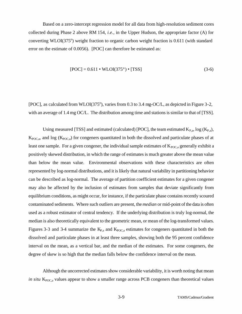
3-9 TAMS/Cadmus/Gradient
Based on a zero-intercept regression model for all data from high-resolution sediment cores
collected during Phase 2 above RM 154, i.e., in the Upper Hudson, the appropriate factor (A) for
converting WLOI(375o) weight fraction to organic carbon weight fraction is 0.611 (with standard
error on the estimate of 0.0056). [POC] can therefore be estimated as:
[POC], as calculated from WLOI(375o), varies from 0.3 to 3.4 mg-OC/L, as depicted in Figure 3-2,
with an average of 1.4 mg OC/L. The distribution among time and stations is similar to that of [TSS].
Using measured [TSS] and estimated (calculated) [POC], the team estimated KP,a, log (KP,a),
KPOC,a, and log (KPOC,a) for congeners quantitated in both the dissolved and particulate phases of at
least one sample. For a given congener, the individual sample estimates of KPOC,a generally exhibit a
positively skewed distribution, in which the range of estimates is much greater above the mean value
than below the mean value. Environmental observations with these characteristics are often
represented by log-normal distributions, and it is likely that natural variability in partitioning behavior
can be described as log-normal. The average of partition coefficient estimates for a given congener
may also be affected by the inclusion of estimates from samples that deviate significantly from
equilibrium conditions, as might occur, for instance, if the particulate phase contains recently scoured
contaminated sediments. Where such outliers are present, the median or mid-point of the data is often
used as a robust estimator of central tendency. If the underlying distribution is truly log-normal, the
median is also theoretically equivalent to the geometric mean, or mean of the log-transformed values.
Figures 3-3 and 3-4 summarize the KP,a and KPOC,a estimates for congeners quantitated in both the
dissolved and particulate phases in at least three samples, showing both the 95 percent confidence
interval on the mean, as a vertical bar, and the median of the estimates. For some congeners, the
degree of skew is so high that the median falls below the confidence interval on the mean.
Although the uncorrected estimates show considerable variability, it is worth noting that mean
in situ KPOC,a values appear to show a smaller range across PCB congeners than theoretical values
[POC] = 0.611 . WLOI(375 ) . [TSS] (3-6) °
3-10 TAMS/Cadmus/Gradient
reported in the literature for partitioning to organic carbon (Figure 3-5). Theoretical values reported
for partitioning to organic carbon for PCB congeners as log (KOC) by Mackay et al. (1992), based on a
relationship to octanol-water partitioning (KOW) range from 4.4 (BZ#1) to 7.3 (BZ#207); mean
estimates of log (KPOC,a) in Figure 3-5 have a smaller range, from 5.0 (BZ#4) to 6.9 (BZ#122).
Direct, uncorrected estimates of both KP,a and KPOC,a show considerable sample-to-sample
variability, which potentially consists of analytical uncertainty, presence of non-equilibrated
conditions, and systematic variability due to environmental conditions. The next section explores the
significant sources of environmental variability in the partition coefficients. Based on this analysis,
appropriate corrections were developed and tested as to predictive ability.
Exploratory Data Analysis of Sources of Variability in Partition Coefficients
The uncorrected KP,a and KPOC,a results presented in the preceding section show a relatively
large amount of variability from sample to sample. Some of the causes of this variability are expected
to be random, others systematic. One component of random variability arises from measurement
imprecision. Bergen et al. (1993) suggest "analytical uncertainty associated with direct water
measurement of PCB congeners is 15-25 percent". Estimating partition coefficients from water
column measurements magnifies any measurement errors: As noted above, estimates of KP,a depend on
the ratio of C P to (C d .[TSS]), while estimates of KPOC,a depend on the ratio of CPto (C d . [POC]).
When C d is close to the practical quantitation limit the measurement precision is relatively low, and
division by a small, imprecise number can translate into a larger error in the estimate of KP,a or K
POC,a. Additional random variability in partition coefficient estimates is introduced by any samples
where the dissolved and particulate phases are not in equilibrium.
Systematic variability in estimates is due to environmental influences. A review of the
literature suggests at least four important potential sources of systematic variability: temperature,
particle concentration, nonlinear adsorption, and changes in the nature of the sorbate, whether
particulates or organic carbon. Salinity may also affect partitioning, but is not a concern in the
freshwater portion of the Hudson.
3-11 TAMS/Cadmus/Gradient
There is relatively little information available in the literature on temperature dependence of
PCB partition coefficients. From thermodynamic considerations, however, equilibrium partition
coefficients are expected to display a clear temperature dependence (Lyman et al., 1990;
Schwarzenbach et al., 1992). Bergen et al. (1993) report that temperature and log (KOW) were
equally important in determining observed values of KP,a for PCB congeners in seawater in New
Bedford Harbor. Various authors have proposed the existence of a particle concentration effect;
however, this may actually represent the influence of the DOC phase, as discussed above. Bierman
(1994) also reports a "general lack of a particle concentration effect" for in situ sediment partition
coefficients for hexachlorobiphenyl and other hydrophobic organic contaminants. Nonlinear
adsorption isotherms are often reported from laboratory experiments. If significantly nonlinear, this
effect would be reflected in a dependence of the partition coefficient on Cd. Impact of sorption to
DOC would also be reflected in a relationship between the observed partition coefficient and Cd,a.
Finally, systematic variations in partition coefficients from sample to sample may be attributable to the
quality of the sorbate. For instance, the makeup of the suspended solids fraction may vary markedly
between spring runoff and summer low-flow conditions. The changes may include both variability in
the mass fraction of organic carbon in solids (which is accounted for in the KPOC approach), and
variability in the nature of the organic carbon, with living plankton biomass accounting for a greater
fraction during the summer.
Two-way analysis of variance (ANOVA) on the calculated partition coefficients by sample
against congener and transect number (time) or station number (location) indicated significant
variability associated with both time and location. Indeed, for estimates of KP,a (but not KPOC,a), the
variation with time overwhelmed variability among congeners. The higher variability in KP,a suggests
that the organic carbon fraction, fOC=[POC]/[TSS], shows significant variability not explained by
variability in [TSS], thus making KPOC,a a better predictor. An analysis of covariance applied to fOC as
a function of station and flow at Fort Edward shows that fOC is significantly correlated to flow, but not
to location, at a 95 percent significance level.
Multiple regression analysis provides additional information on significant contributors to
variability in observed partition coefficients. The explanatory variables considered were
temperature, [TSS], [DOC], flow (at Fort Edward), and dissolved-phase concentration of the PCB
congener. Thermodynamic considerations suggest an approximately linear relationship between the
3-12 TAMS/Cadmus/Gradient
natural log of the partition coefficient and temperature (as discussed below). The team also
investigated linear, log-linear and log-log relationships between partition coefficients and [DOC] and
[TSS] (or their inverses), and flow. Step-wise multiple regression (run both forward and backward)
indicated which variables had significant explanatory power (using a 95 percent significance criterion
for variables to be included in or excluded from the model). As this was primarily a scoping exercise,
the identification of significant variables is more important than the exact form of the model (except
that predictors highly correlated to one another may obscure causal relationships, as described
below). The team examined the behavior of partition coefficients (both KP,a and K POC,a) for ten key
congeners, representing a range of environmental properties. The results are shown in Tables 3-1
and 3-2. In these tables, a blank indicates the lack of statistically significant explanatory power, while
a + or - indicates a significant relationship, with sign.
From these tables, there is, first, very little evidence of any significant relationship between
partition coefficients and dissolved concentration or [DOC]. Most of the KP,a values have a strong
negative relationship to [TSS]; however, this relationship disappears when normalized to an organic
carbon basis, suggesting that a particle concentration effect is not significant following normalization
to [POC] over the range of environmental conditions sampled in the Hudson. Lack of a strong
relationship between KPOC,a and either [DOC] or [TSS] suggests that variability in fraction sorbed to
DOC also does not have a major effect on the particle-sorbed concentrations for most congeners,
within the limited range of observed [DOC].
Significant negative relationships of partition coefficients to temperature are seen in the
regression results for log(KP,a) and, for some congeners, for log (KPOC,a). Interpretation of the results
is aided by examining the correlation pattern among the explanatory variables. Where these are highly
correlated with one another, the impact of one variable may mask or substitute for that of another. The
correlations among [DOC], temperature, [TSS], and flow vary from congener to congener (differing
largely on the basis of available samples). Table 3-3 shows correlation structures among the
independent variables used to predict partition coefficients. Flow is negatively correlated with
temperature and [DOC] (the highest flows occurred coincident with the lowest water temperatures and
lowest DOC concentrations during snowmelt runoff); thus the positive correlation between flow and
KPOC,a for BZ#28, BZ#118, and BZ#138 shown in Table 3-2 may actually reflect a negative
correlation to temperature. Indeed, the sign of the regression coefficient on flow is always positive
3-13 TAMS/Cadmus/Gradient
for KPOC,a, but is not statistically significant for most congeners, while the regression coefficient on
[DOC] is never statistically significant. Figure 3-6 shows the general trend for calculated values of
KPOC,a versus temperature for BZ#52. A trend of decreasing K POC,a with increasing temperature is
visible, although appearing to represent only a small part of the total variability in observed
partitioning behavior. In sum, the exploratory data analysis suggests that the influence of temperature
should be investigated in the analysis of PCB partitioning in the Hudson River.
Additional qualitative information on variability in partition coefficients is provided by visual
examination of plots of estimated partition coefficients versus location and time. Figures 3-7
through 3-10 show log (KP,a) and log (KPOC,a) values for BZ#44 plotted against transect number and
station (for the Upper Hudson between RM 195.5 in the remnant deposit area and RM 156.5 near
Waterford). Both KP,a and KPOC,a tend to lower values during Transect 6, when temperatures were
highest, and flows lowest. The trend is clearer for KPOC,a.
Noticeable in all transects are the generally consistent values for KP,a and KPOC,a estimates for
most congeners within a given transect beginning at Station 5, the TI Dam (RM 188.5). This suggests
that approximate equilibrium conditions are established within the Pool and remain consistent
throughout the remainder of the freshwater Hudson (with the possible exception of mono- and di-
chlorinated congeners, as discussed further below). The results for Rogers Island, Station 4, are
distinctly different from those downstream and probably reflect its proximity to the Hudson Falls
source resulting in a lack of water column equilibrium. Also notable in Figures 3-9 and 3-10 is the
degree of variability within transects as opposed to among transects. In general, there is less
variability within a given transect downstream of Station 5 than there is among the transects at any
given station beginning with Station 5. This suggests that the factors influencing the partition
coefficients, e.g., temperature and the nature of the POC, are largely consistent within a transect, but
the variation of these factors among transects causes the differing partition coefficients.
In sum, the exploratory analysis suggests that significant variability in partition coefficients is
related in part to water temperature changes. Apparent particle concentration effects are significant
for KP,a, but appear to be removed by correction to an organic carbon basis. Some samples,
particularly those collected at RM 194.6, may exhibit temporary disequilibrium between dissolved
and particulate phases. Finally, partition coefficients are most consistent in the region beginning at the
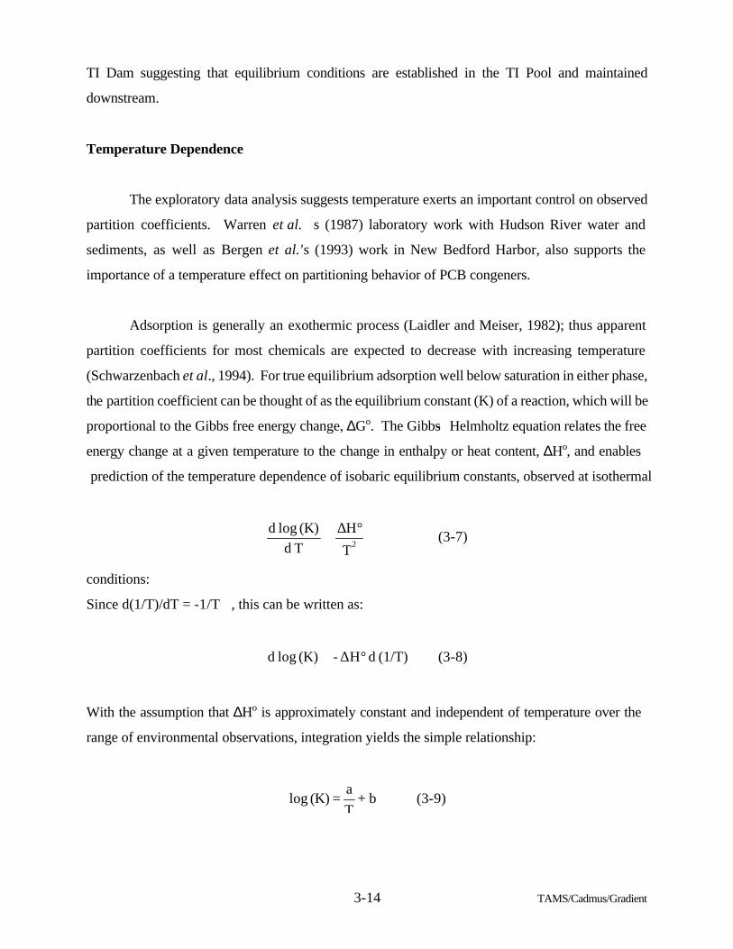
3-14 TAMS/Cadmus/Gradient
TI Dam suggesting that equilibrium conditions are established in the TI Pool and maintained
downstream.
Temperature Dependence
The exploratory data analysis suggests temperature exerts an important control on observed
partition coefficients. Warren et al.�s (1987) laboratory work with Hudson River water and
sediments, as well as Bergen et al.'s (1993) work in New Bedford Harbor, also supports the
importance of a temperature effect on partitioning behavior of PCB congeners.
Adsorption is generally an exothermic process (Laidler and Meiser, 1982); thus apparent
partition coefficients for most chemicals are expected to decrease with increasing temperature
(Schwarzenbach et al., 1994). For true equilibrium adsorption well below saturation in either phase,
the partition coefficient can be thought of as the equilibrium constant (K) of a reaction, which will be
proportional to the Gibbs free energy change, ∆Go. The Gibbs- Helmholtz equation relates the free
energy change at a given temperature to the change in enthalpy or heat content, ∆Ho , and enables
prediction of the temperature dependence of isobaric equilibrium constants, observed at isothermal
conditions:
Since d(1/T)/dT = -1/T�, this can be written as:
With the assumption that ∆Ho is approximately constant and independent of temperature over the
range of environmental observations, integration yields the simple relationship:
T
H
T d
(K) log d2
°∆∝ (3-7)
(1/T) d H- (K) log d °∆∝ (3-8)
b + T
a = (K) log (3-9)
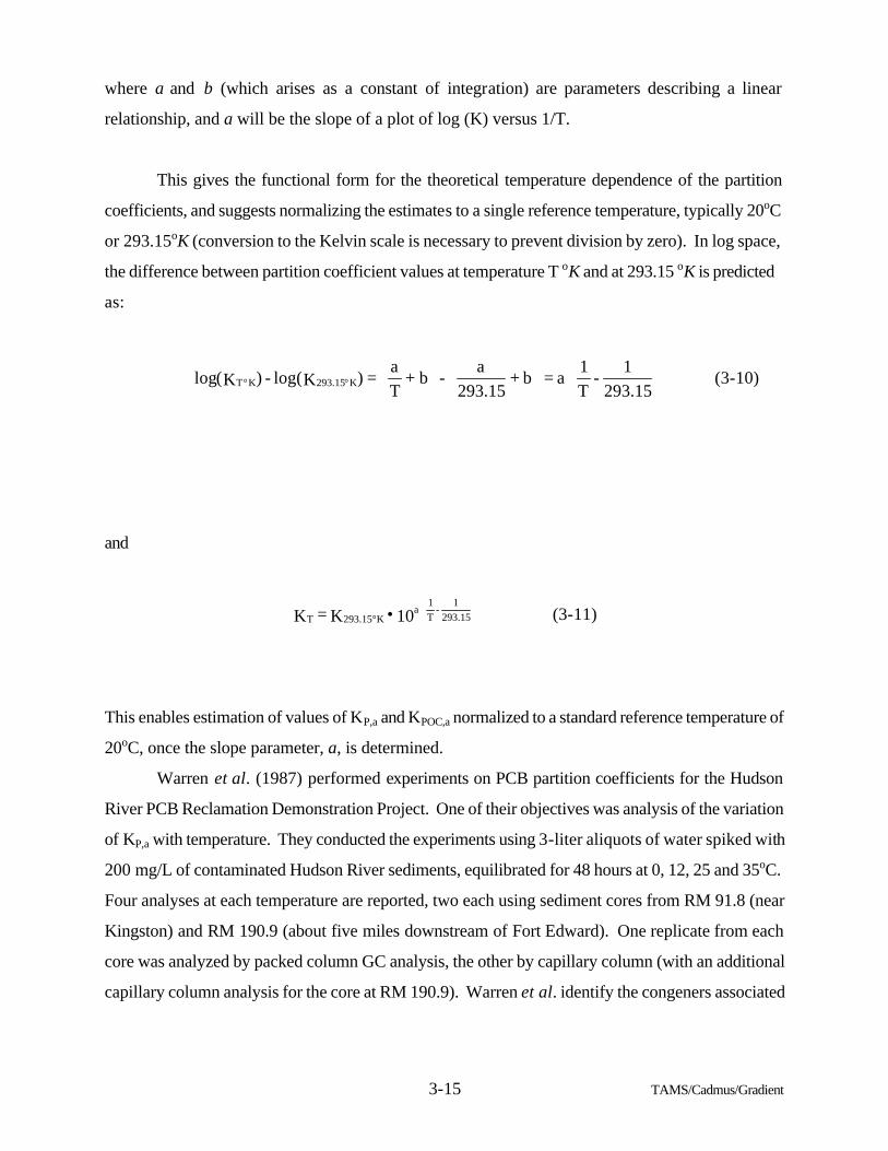
3-15 TAMS/Cadmus/Gradient
where a and b (which arises as a constant of integration) are parameters describing a linear
relationship, and a will be the slope of a plot of log (K) versus 1/T.
This gives the functional form for the theoretical temperature dependence of the partition
coefficients, and suggests normalizing the estimates to a single reference temperature, typically 20oC
or 293.15oK (conversion to the Kelvin scale is necessary to prevent division by zero). In log space,
the difference between partition coefficient values at temperature T oK and at 293.15 oK is predicted
as:
and
This enables estimation of values of KP,a and KPOC,a normalized to a standard reference temperature of
20oC, once the slope parameter, a, is determined.
Warren et al. (1987) performed experiments on PCB partition coefficients for the Hudson
River PCB Reclamation Demonstration Project. One of their objectives was analysis of the variation
of KP,a with temperature. They conducted the experiments using 3-liter aliquots of water spiked with
200 mg/L of contaminated Hudson River sediments, equilibrated for 48 hours at 0, 12, 25 and 35oC.
Four analyses at each temperature are reported, two each using sediment cores from RM 91.8 (near
Kingston) and RM 190.9 (about five miles downstream of Fort Edward). One replicate from each
core was analyzed by packed column GC analysis, the other by capillary column (with an additional
capillary column analysis for the core at RM 190.9). Warren et al. identify the congeners associated
°°293.15
1 -
T
1a = b +
293.15
a - b +
T
a = )K(log - )K(log K293.15KT (3-10)
10 K = K 293.15
1 -
T
1a
K293.15T
° • (3-11)
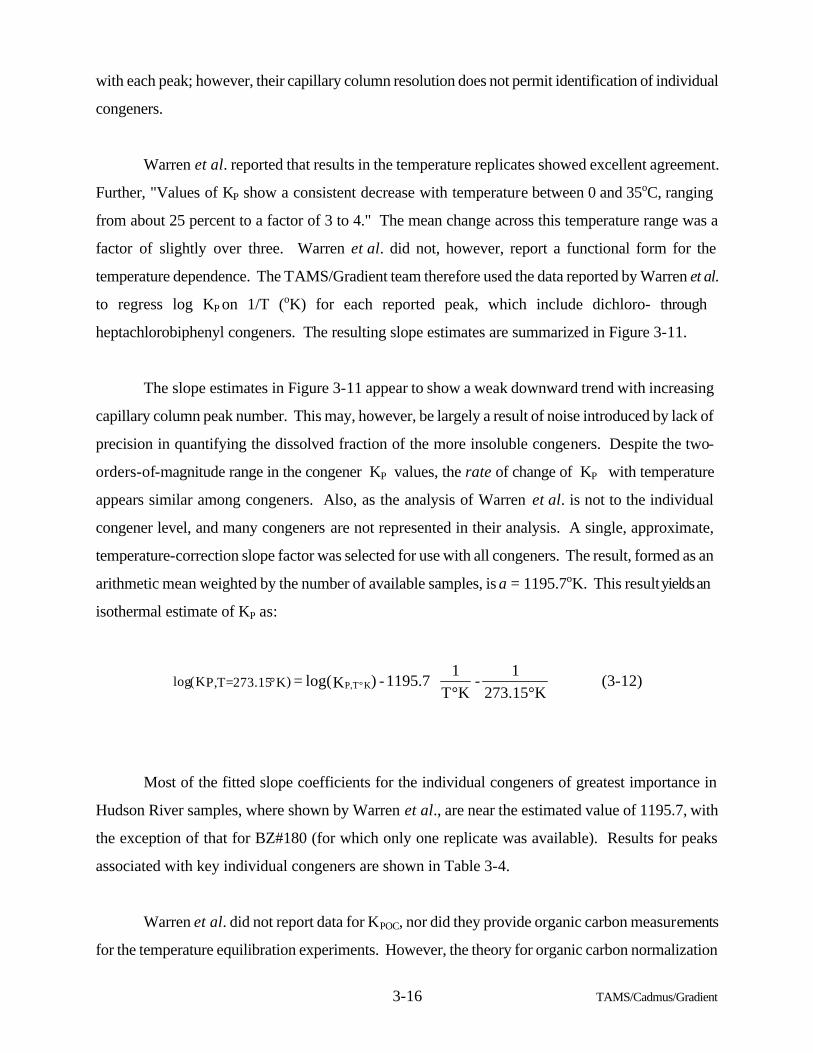
3-16 TAMS/Cadmus/Gradient
with each peak; however, their capillary column resolution does not permit identification of individual
congeners.
Warren et al. reported that results in the temperature replicates showed excellent agreement.
Further, "Values of KP show a consistent decrease with temperature between 0 and 35oC, ranging
from about 25 percent to a factor of 3 to 4." The mean change across this temperature range was a
factor of slightly over three. Warren et al. did not, however, report a functional form for the
temperature dependence. The TAMS/Gradient team therefore used the data reported by Warren et al.
to regress log KP on 1/T (oK) for each reported peak, which include dichloro- through
heptachlorobiphenyl congeners. The resulting slope estimates are summarized in Figure 3-11.
The slope estimates in Figure 3-11 appear to show a weak downward trend with increasing
capillary column peak number. This may, however, be largely a result of noise introduced by lack of
precision in quantifying the dissolved fraction of the more insoluble congeners. Despite the two-
orders-of-magnitude range in the congener KP values, the rate of change of KP with temperature
appears similar among congeners. Also, as the analysis of Warren et al. is not to the individual
congener level, and many congeners are not represented in their analysis. A single, approximate,
temperature-correction slope factor was selected for use with all congeners. The result, formed as an
arithmetic mean weighted by the number of available samples, is a = 1195.7oK. This result yields an
isothermal estimate of KP as:
Most of the fitted slope coefficients for the individual congeners of greatest importance in
Hudson River samples, where shown by Warren et al., are near the estimated value of 1195.7, with
the exception of that for BZ#180 (for which only one replicate was available). Results for peaks
associated with key individual congeners are shown in Table 3-4.
Warren et al. did not report data for KPOC, nor did they provide organic carbon measurements
for the temperature equilibration experiments. However, the theory for organic carbon normalization
°°°°K273.15
1 -
KT
1 1195.7 - )K(log = KTP,)K K273.15=TP,(log (3-12)
3-17 TAMS/Cadmus/Gradient
is that the observed partitioning is controlled by the organic fraction of particulates, and the same
mechanism applies for estimates of KP and KPOC. Thus, the temperature correction slope should be
approximately equal for KP,a and KPOC,a, since they are related by a single, non-temperature dependent
constant, foc (see Equation 3.4). Thus, the same temperature correction can be applied to KPOC,a.
Evaluation of Equilibrium Assumptions
Equilibrium partitioning models assume that environmental samples display equilibration
between the different phases. It is expected that at least some samples will represent non-equilibrium
conditions. An analysis of the apparent degree of equilibration is thus important to interpretation of
in situ equilibrium partition coefficients from the data.
Analysis of Equilibrium Samples
In the equilibration study, duplicate water column transect samples were collected and held for
approximately four days prior to filtration and analysis for the purpose of determining whether PCB-
congener concentrations in the dissolved and suspended-matter phases were at equilibrium in the
water column. Significant changes between the instantaneous transect samples and the equilibrated
samples could indicate that a true equilibrium did not exist in the water column. While changes
between transect and equilibration results were noted, the experimental design did not call for
maintenance of a specific ambient temperature during equilibration and observed changes may be due
to temperature effects; thus the evidence on in situ equilibrium is unclear.
The TAMS/Gradient team collected equilibration samples during Transects 2 and 6.
Transect 2 represents winter conditions, while Transect 6 represents summer conditions. The
differences between the transect and equilibration values of KP,a are summarized separately for the
two sets of equilibration data, on a log scale, in Figure 3-12. KP,a values for the Transect 2 samples
are, on the average, higher than the corresponding values for the equilibrated samples. For the
Transect 6 samples, the values of KP,a are generally less than the estimates from the equilibrated
samples. The Transect 6 results match results obtained from paired large-volume filter studies
conducted at Mechanicville in 1983 (Bopp et al., 1985). Essentially the same relationships
as are seen for Kp in the two transects are seen for KPOC,a estimates, so the differences are not solely
attributable to differing organic carbon content of particulate matter for the two transects.
3-18 TAMS/Cadmus/Gradient
The Transect 2 equilibration samples might be interpreted to suggest that the PCB mass was
generally out of equilibrium toward the particulate phase. In Transect 6, the PCB mass generally
appears out of equilibrium toward the dissolved phase. There is, however, a confounding factor in
the interpretation, as the samples were not held at their original ambient temperature during
equilibration. In the discussion of temperature dependence, it is clear that there is a strong inverse
relationship between partition coefficients and temperature. Transect 2 samples were taken during
cold weather and Transect 6 samples during warm weather. The equilibration process thus involved
some warming of the Transect 2 samples, and cooling of the Transect 6 samples, which should
produce, respectively, decreases and increases in Kd values. This temperature change alone could
account for the observed shifts in Kp values during equilibration.
Evidence for Disequilibrium in Transect Observations
Despite the inconclusive interpretation of the equilibration experiments, a number of individual
samples clearly represent non-equilibrium conditions, and are thus not appropriate for the calculation
of equilibrium partition coefficients. The presence of a certain proportion of samples out of
equilibrium is expected. For instance, samples collected during a non-scouring period where
significant release of dissolved PCBs was occurring from the sediment would be out of equilibrium
toward the dissolved phase until sufficient time passed for equilibration to occur with suspended
solids. Conversely, during scour events which mobilize sediment-bound PCBs, the water column
samples may be temporarily out of equilibrium toward the particulate phase until the PCBs in the
particulate and dissolved phases reach equilibrium. Tributaries loading relatively clean water or
sediment may also cause temporary disequilibrium.
While it is not appropriate to include non-equilibrated samples in the estimation of
equilibrium partition coefficients, there is no clear a priori criterion to determine which samples are
inappropriate. This situation calls for estimators which are more robust to the presence of
inappropriate or outlying data than the mean. As noted above, a useful estimator of central tendency in
such situations is the median, or 50th percentile of the observations, which is much less affected by
outliers than the mean.
3-19 TAMS/Cadmus/Gradient
Upper Versus Lower River Estimates
Initial estimates of partition coefficients were based on transect data from the Upper Hudson
only, due to potential differences in the nature of sorbate below the confluence with the Mohawk
River. However, there are also reasons for the inclusion of freshwater Lower Hudson samples into
the analysis (if consistent differences do not apply). Given the high variability in partition coefficient
estimates in individual Upper Hudson samples, the increased sample size resulting from adding the
Lower Hudson samples would be helpful for calculation of average values.
Lower Hudson samples are available for Transects 1, 4, and 6 only, and Transect 1 included
Lower Hudson samples at RM 153 (Green Island) and RM 102 (Cementon) only (the latter station was
not used in subsequent transects). There is generally more variability in partition coefficient estimates
between transects than between stations within a transect. The behavior of apparent partition
coefficient values in these transects can be compared between the Upper and Lower Hudson and
examined for a representative suite of congeners. For Transect 1, collected in January and February,
KP,a estimates appear to decline gradually downriver, with the biggest change occurring in the more-
chlorinated congeners (Figure 3-13). The difference between estimates at RM 188.5 (the TI Dam) and
RM 156.6 (Waterford), however, is greater than that between Waterford and the Lower Hudson
stations, and may be partly attributable to temperature changes.
In Transect 4 (Figure 3-14), conducted in April, apparent KP,a values again declined with river
mile in the Upper Hudson, but there does not appear to be a systematic change from the Upper to the
Lower Hudson. During Transect 6 (Figure 3-15), partitioning at Waterford (RM 156.6) is again very
similar to that in the freshwater portion of the lower Hudson.
There does appear to be a difference in the partitioning behavior of more highly chlorinated
versus less chlorinated PCB congeners with location in the Hudson. Figure 3-16 summarizes the
average percent deviations from the mean for congener KPOC,a estimates by station, with mono- through
tri-chlorinated congeners and tetra- and higher-chlorinated congeners represented separately. All
congeners tend to show increased estimates of KPOC,a at RM 196.8 (Rogers Island), which may
represent presence of non-equilibrated sediment in the samples. Above and below RM 196.8, KPOC,a
estimates for the more chlorinated congeners are relatively constant. For the mono- through tri-
chlorinated congeners, KPOC,a estimates are at a minimum at RM 188.5 (TI Dam), then tend to increase
3-20 TAMS/Cadmus/Gradient
steadily downstream. This may indicate loading of a predominantly dissolved-phase (or DOC-bound)
mass of lower-chlorinated congeners within the TI Pool, coupled with gradual adsorption and
volatilization loss of the dissolved phase, and coagulation and conversion to particulate form of the
DOC-bound phase (Buffle and Leppard, 1995) as flow proceeds downstream. There does not,
however, appear to be a significant change in partitioning behavior across the boundary between the
Upper and Lower Hudson. Indeed, including both upper and lower river estimates may aid in
compensating for any bias introduced by local disequilibrium in the area of the TI Pool.
In sum, the available data suggest no clear distinction between partitioning behavior in the
Upper Hudson and partitioning behavior in the freshwater portion of the Lower Hudson. Changes
between stations within the Upper Hudson are likely attributable to variations in organic carbon
concentration and water temperature. Use of samples from the freshwater portion of the Lower
Hudson provides advantages of larger sample size. These samples were therefore included in the
analysis of partition coefficients.
Corrected Two-Phase Partition Coefficients for Application
The discussions in the preceding sections suggest that partition coefficients should be
estimated on a temperature-normalized basis (20oC), using the temperature correction factor
described in Equation (3-12). In addition, data should be summarized across all main-stem samples
between the remnant deposits and the salt front, using the arithmetic median to avoid undue influence
from outliers and non-equilibrated samples.
The ability to predict particulate-phase congener concentrations from dissolved-
phase observations using a squared error criterion provides a basis for evaluating the relative
performance of different formulations of the two-phase partition coefficient. That is, estimates of the
particulate-phase concentration can be predicted from CPOC = KPOC,a @ [POC] @ Cd and C P = KP,a @
[TSS] @ Cd and compared to observations. Table 3-5 shows the relative performance across all
congeners for which partition coefficients could be estimated. Figures 3-17 and 3-18 show the
performance of temperature-corrected KP,a and KPOC,a estimates in predicting CP from Cd,a for those
congeners quantitated in both phases in at least three samples. Estimates of CP using KP,a appear to
have limited predictive power, and predicted values fall into two distinct groups, one above and one
below the line of perfect fit. In contrast, most KPOC,a-based predictions fall relatively close to and
3-21 TAMS/Cadmus/Gradient
evenly distributed about the unit line. A small subset of KPOC,a-based predictions are substantially
under-predicted. These represent samples which were significantly out of equilibrium toward the
dissolved phase. Because median values were used to estimate KPOC,a, these outliers have little effect
on the reported estimates.
The results in Table 3-5 indicate that a substantial improvement in predictive ability is
obtained by using KPOC,a instead of KP,a, despite any additional noise introduced in the estimate of
[POC]. Further improvements are gained by introducing a temperature correction, and using the
median estimate to reduce the influence of non-equilibrated outliers. The TAMS/Gradient team
therefore recommends using median values of in situ KPOC,a estimates with a correction to a reference
temperature of 20oC as the basis for two-phase models of PCB congener fate and transport.
The resulting estimates of KPOC,a and log(K POC,a) are presented in Table 3-6(a) and 3-6(b), and
summarized in Figure 3-19.
The temperature-corrected KPOC,a estimates provide a relatively good ability to predict
concentrations of PCBs in one phase from those in the other. The average absolute percent difference
between observed and predicted concentrations in the particulate phase for all congeners was 43
percent. For the Upper Hudson River from RM 188.5 (Station 5, TI Dam) to RM 156.6 (Station 8,
Waterford), more than half of the estimates of particulate-phase concentrations from dissolved-phase
concentrations were within 28 percent of measured values. Further, the quality of prediction was high
even at Station 8 during Transect 3, where substantial quantities of PCBs appear to have been
mobilized by a localized scour event in the reach above the station (see Subsection 3.2.5 for
discussion). In these samples, the median percent difference between observed and predicted CPOC
was 22 percent and discrepancies that do exist may be attributable to an atypical composition of the
POC fraction during this high suspended-load event.
Average percent differences between observed and predicted values differ considerably
among congeners. For congeners detected in both particulate and dissolved phases in at least ten
samples at Stations 5 through 8, the average absolute percent difference is as low as 18 percent for
BZ#101 and less than 50 percent for all congeners except BZ#1. High average percent differences for
BZ#1 (98 percent) may reflect difficulties in quantitating this congener, as well as potential
disequilibrium in some samples. At upstream stations nearer the GE Hudson Falls source (Stations 3
3-22 TAMS/Cadmus/Gradient
and 4), the average percent differences are, on average, 1.8 times those for Stations 5 through 8. This
suggests that PCBs in the water column may not have reached an equilibrium distribution between
phases prior to reaching the head of the TI Pool.
The quality of fit can also be summarized via the sample standard deviations of the estimates
of log(KPOC,a). These range from 0.029 to 0.55 log units in this study, with most in the range of 0.2 to
0.3 log units. Across all congeners, the average standard deviation in estimates of log(KPOC,a) is 0.276
and the median 0.244 log units. These results compare favorably with other studies reported in the
literature. Bergen et al. (1993), studying six PCB congeners at four stations in New Bedford Harbor,
reported standard deviations for estimates of log(KPOC,a) ranging from 0.25 to 0.50 log units. Bierman
et al. (1992) analyzed five congener groups in Green Bay and reported standard deviations for
estimates of log(KPOC,a) ranging from 0.27 to 0.36 log units. Finally, Baker et al. (1986) reported
standard deviations ranging from 0.1 to 0.9 for log(KPOC,a) estimates for 28 congeners in Lake
Superior, with an average standard deviation of approximately 0.5 log units.
Evaluation of Partitioning in the Flow-Averaged Samples
The flow-averaged samples were collected for the purpose of estimating PCB flux over time,
and represent a flow-weighted average water concentration for a 15-day period. These samples were
analyzed for dissolved and particulate concentrations, but were intended to provide estimates of total
flux of a given congener.
Because of the sample collection and handling methodology, the phase distribution of PCB
congeners in the flow-averaged samples may not be representative of the instream phase distribution.
First, the samples are composites of instantaneous sub-samples which have been held for varying
lengths of time. If the older sub-samples were initially out of equilibrium, the long holding time
allows for movement toward equilibrium. More importantly, the flow-averaged samples mix sub-
samples with varying initial concentrations of PCBs, [TSS], [POC] and [DOC]. Thus the composite
mixture may show a phase distribution quite different from any of the instantaneous sub-samples.
However, if the transect sample analysis does yield valid estimates of equilibrium partition
coefficients, similar results, on average, should be obtained from the flow-averaged samples. In sum,
3-23 TAMS/Cadmus/Gradient
the flow-averaged samples cannot be used to calculate valid in situ partition coefficients, but can be
used as a check on reasonableness of the estimates.
A temperature correction is not possible for the flow-averaged samples, because the
individual sub-samples were collected at differing temperatures, and the composite was held on ice,
not at a temperature reflecting a weighted average of collection temperatures. As noted above, a
correction to a POC basis does improve accuracy of estimation of partitioning, and it is most
appropriate to compare the median of flow-averaged KPOC,a estimates to transect K POC,a estimates.
Figure 3-20 compares the medians of the flow-averaged KPOC,a estimates for the entire flow-
averaged sampling program to the transect median estimates (normalized to 20oC). This shows that
estimated partition coefficients in the flow-averaged samples are similar to those obtained from the
transect samples. In sum, the flow-averaged samples confirm the order of magnitude of the KPOC,a
estimates from the transect samples. They should not, however, be assumed to provide accurate
estimates of the in situ phase distribution of PCB congeners. Instead, the flow-averaged samples are
best used, as intended, to assess the total flux of congeners.
3.1.2 Three-Phase Models of Equilibrium Partitioning
Laboratory experiments (e.g., Carter and Suffet, 1982; Gschwend and Wu, 1985), as well as
field observations (e.g., Baker et al., 1986; Means and Wijayaratne, 1982) have demonstrated that a
two-phase model of equilibrium partitioning may not be optimal for hydrophobic organic pollutants.
That is, such compounds sorb not just to filterable particulate organic matter, but also to colloidal-size
and dissolved organic matter, such as humic and fulvic acids, which may play a significant role in
facilitating transport (see review of Sigleo and Means, 1990). The fraction sorbed to the non-
filterable organic carbon represents a third-phase, which is neither sorbed to particulates (as defined
by filtration) nor truly dissolved. Analytically, this fraction is resolved and reported as part of the
"dissolved" phase; however, considering it to be truly dissolved may result in a misrepresentation of
phase partitioning behavior if significant variability occurs in the concentration of "dissolved" organic
carbon (i.e., the organic carbon content which is not filterable) occurs.
3-24 TAMS/Cadmus/Gradient
The presence of a significant third phase may have important implications for biotic uptake, as
dissolved constituents are generally thought to be more readily bioavailable than those sorbed to
DOC. DOC is consistently present in samples of Hudson River water at levels around 4 mg/L.
Further, for many PCB congeners, a larger fraction of total mass in a sample is seen in the analytical
"dissolved" phase than in the particulate phase. For instance, 73 percent of the mass of BZ#18 is, on
average, reported in the "dissolved" phase. This percentage declines with increasing KPOC,a, and for
BZ#153 only about 36 percent of the mass is in the "dissolved" phase.
Whether or not the DOC-bound phase has a significant effect on the environmental distribution
of compounds in the water column depends on [DOC] and the hydrophobicity of the compound. Eadie
et al. (1992) found in Lake Ontario that the DOC-bound phase accounted for 10 percent or less of total
water column mass for hexachlorobiphenyls and compounds of similar hydrophobicity. Brownawell
and Achman (1994) reported that colloidal materials did not appear to have a significant effect on
water column partitioning for most PCB congeners in the Hudson estuary, except for the most
hydrophobic PCBs. Bierman et al. (1992) in the Green Bay PCBs study estimated that the water
column DOC-bound fraction for congeners BZ#28, 31, 56, 60, 101, 138, 158, and 163 was on the
order of 2 percent to 3 percent. (This result was based on an assumption that KDOC = 0.01 @ KPOC,
rather than an independent determination of KDOC.) For porewater, in contrast, Burgess et al. (1996)
report that the DOC-bound fraction of PCB congeners in New Bedford Harbor ranged from 40 percent
for dichlorobiphenyls to greater than 80 percent for tetra- through octa-chlorinated PCBs.
Three-Phase Partitioning Theory
To evaluate the significance of a DOC-bound phase of PCBs in the water column of the
Hudson River, three-phase models of partitioning can be employed, which explicitly account for the
DOC-bound fraction. But, because the third, DOC-bound phase is not readily observable and was not
measured in the Phase 2 study, this presents significant problems for the determination of in situ
partition coefficients. This section presents several attempts to fit three-phase partition coefficients,
and uses this evidence to evaluate the significance of the third (DOC) phase for modeling the behavior
of PCBs in the Hudson River.
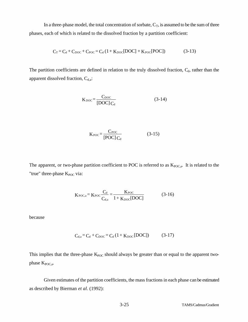
3-25 TAMS/Cadmus/Gradient
In a three-phase model, the total concentration of sorbate, CT, is assumed to be the sum of three
phases, each of which is related to the dissolved fraction by a partition coefficient:
The partition coefficients are defined in relation to the truly dissolved fraction, Cd, rather than the
apparent dissolved fraction, Cd,a:
The apparent, or two-phase partition coefficient to POC is referred to as KPOC,a. It is related to the
"true" three-phase KPOC via:
because
This implies that the three-phase KPOC should always be greater than or equal to the apparent two-
phase KPOC,a.
Given estimates of the partition coefficients, the mass fractions in each phase can be estimated
as described by Bierman et al. (1992):
[POC])K + [DOC]K + (1 C = C + C + C = C POCDOCdPOCDOCdT (3-13)
C[DOC]C = K
d
DOCDOC (3-14)
C[POC]C = K
d
POCPOC (3-15)
[DOC]K + 1K =
C
C K = KDOC
POC
d,a
dPOCPOC,a (3-16)
[DOC]) K + (1 C = C + C = C DOCdDOCdd,a (3-17)
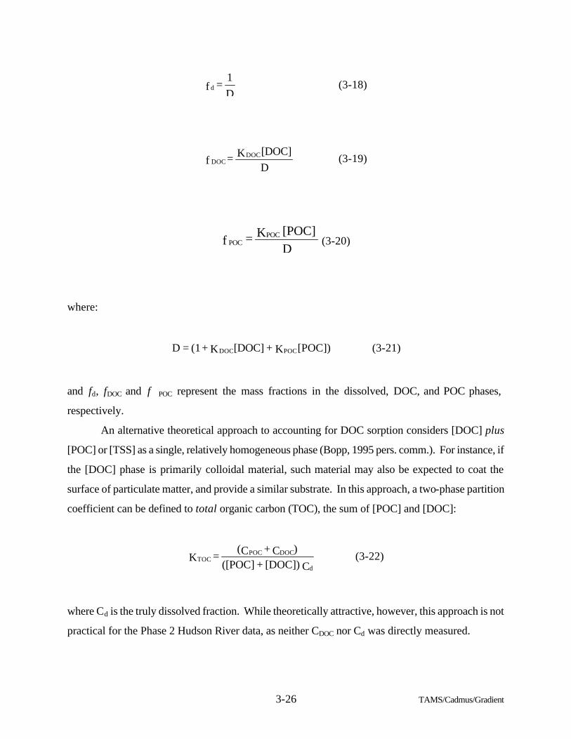
3-26 TAMS/Cadmus/Gradient
where:
and fd, fDOC and f POC represent the mass fractions in the dissolved, DOC, and POC phases,
respectively.
An alternative theoretical approach to accounting for DOC sorption considers [DOC] plus
[POC] or [TSS] as a single, relatively homogeneous phase (Bopp, 1995 pers. comm.). For instance, if
the [DOC] phase is primarily colloidal material, such material may also be expected to coat the
surface of particulate matter, and provide a similar substrate. In this approach, a two-phase partition
coefficient can be defined to total organic carbon (TOC), the sum of [POC] and [DOC]:
where Cd is the truly dissolved fraction. While theoretically attractive, however, this approach is not
practical for the Phase 2 Hudson River data, as neither CDOC nor Cd was directly measured.
D
1 = f d (3-18)
D
[DOC] K = fDOC
DOC (3-19)
D
[POC] K = fPOC
POC (3-20)
[POC])K + [DOC]K + (1 = D POCDOC (3-21)
C [DOC]) + ([POC]
)C + C( = Kd
DOCPOCTOC (3-22)
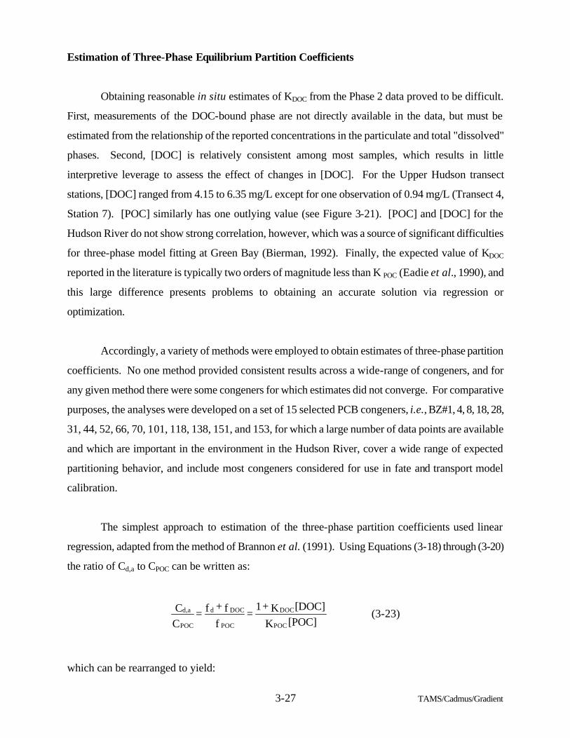
3-27 TAMS/Cadmus/Gradient
Estimation of Three-Phase Equilibrium Partition Coefficients
Obtaining reasonable in situ estimates of KDOC from the Phase 2 data proved to be difficult.
First, measurements of the DOC-bound phase are not directly available in the data, but must be
estimated from the relationship of the reported concentrations in the particulate and total "dissolved"
phases. Second, [DOC] is relatively consistent among most samples, which results in little
interpretive leverage to assess the effect of changes in [DOC]. For the Upper Hudson transect
stations, [DOC] ranged from 4.15 to 6.35 mg/L except for one observation of 0.94 mg/L (Transect 4,
Station 7). [POC] similarly has one outlying value (see Figure 3-21). [POC] and [DOC] for the
Hudson River do not show strong correlation, however, which was a source of significant difficulties
for three-phase model fitting at Green Bay (Bierman, 1992). Finally, the expected value of KDOC
reported in the literature is typically two orders of magnitude less than K POC (Eadie et al., 1990), and
this large difference presents problems to obtaining an accurate solution via regression or
optimization.
Accordingly, a variety of methods were employed to obtain estimates of three-phase partition
coefficients. No one method provided consistent results across a wide-range of congeners, and for
any given method there were some congeners for which estimates did not converge. For comparative
purposes, the analyses were developed on a set of 15 selected PCB congeners, i.e., BZ#1, 4, 8, 18, 28,
31, 44, 52, 66, 70, 101, 118, 138, 151, and 153, for which a large number of data points are available
and which are important in the environment in the Hudson River, cover a wide range of expected
partitioning behavior, and include most congeners considered for use in fate and transport model
calibration.
The simplest approach to estimation of the three-phase partition coefficients used linear
regression, adapted from the method of Brannon et al. (1991). Using Equations (3-18) through (3-20)
the ratio of Cd,a to CPOC can be written as:
which can be rearranged to yield:
[POC] K
[DOC] K + 1 =
f
f + f = C
C
POC
DOC
POC
DOCd
POC
d,a (3-23)
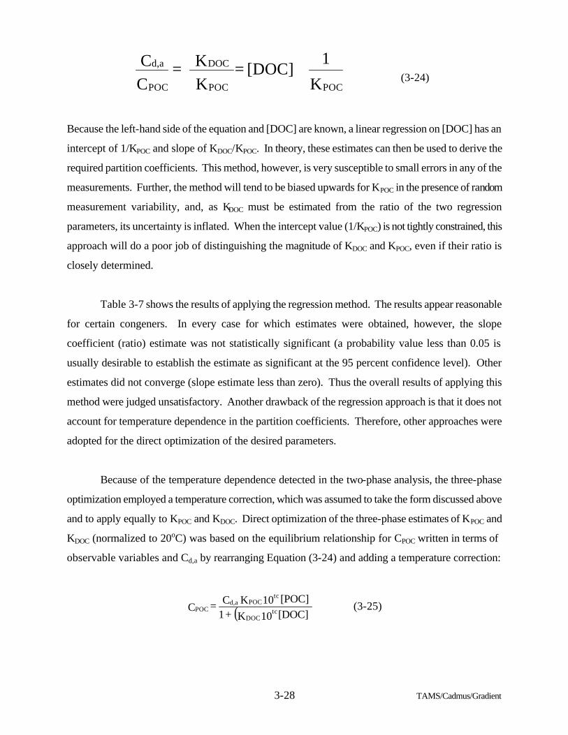
3-28 TAMS/Cadmus/Gradient
Because the left-hand side of the equation and [DOC] are known, a linear regression on [DOC] has an
intercept of 1/KPOC and slope of KDOC/KPOC. In theory, these estimates can then be used to derive the
required partition coefficients. This method, however, is very susceptible to small errors in any of the
measurements. Further, the method will tend to be biased upwards for KPOC in the presence of random
measurement variability, and, as KDOC must be estimated from the ratio of the two regression
parameters, its uncertainty is inflated. When the intercept value (1/KPOC) is not tightly constrained, this
approach will do a poor job of distinguishing the magnitude of KDOC and KPOC, even if their ratio is
closely determined.
Table 3-7 shows the results of applying the regression method. The results appear reasonable
for certain congeners. In every case for which estimates were obtained, however, the slope
coefficient (ratio) estimate was not statistically significant (a probability value less than 0.05 is
usually desirable to establish the estimate as significant at the 95 percent confidence level). Other
estimates did not converge (slope estimate less than zero). Thus the overall results of applying this
method were judged unsatisfactory. Another drawback of the regression approach is that it does not
account for temperature dependence in the partition coefficients. Therefore, other approaches were
adopted for the direct optimization of the desired parameters.
Because of the temperature dependence detected in the two-phase analysis, the three-phase
optimization employed a temperature correction, which was assumed to take the form discussed above
and to apply equally to KPOC and KDOC. Direct optimization of the three-phase estimates of KPOC and
KDOC (normalized to 20oC) was based on the equilibrium relationship for CPOC written in terms of
observable variables and Cd,a by rearranging Equation (3-24) and adding a temperature correction:
K
1[DOC]
K
K = C
C
POCPOC
DOC
POC
d,a += (3-24)
( )[DOC] 10 K + 1
[POC] 10 K C = C tcDOC
tcPOCd,a
POC (3-25)
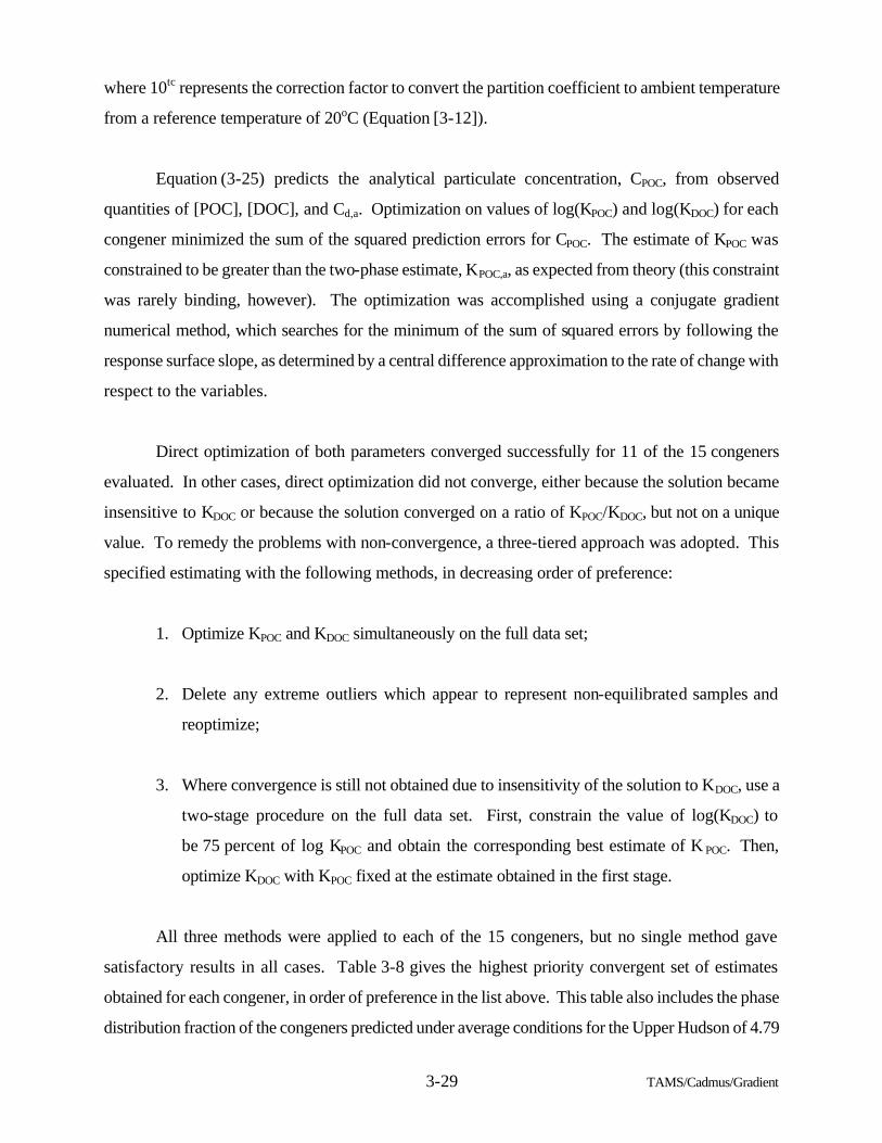
3-29 TAMS/Cadmus/Gradient
where 10tc represents the correction factor to convert the partition coefficient to ambient temperature
from a reference temperature of 20oC (Equation [3-12]).
Equation (3-25) predicts the analytical particulate concentration, CPOC, from observed
quantities of [POC], [DOC], and Cd,a. Optimization on values of log(KPOC) and log(KDOC) for each
congener minimized the sum of the squared prediction errors for CPOC. The estimate of KPOC was
constrained to be greater than the two-phase estimate, KPOC,a, as expected from theory (this constraint
was rarely binding, however). The optimization was accomplished using a conjugate gradient
numerical method, which searches for the minimum of the sum of squared errors by following the
response surface slope, as determined by a central difference approximation to the rate of change with
respect to the variables.
Direct optimization of both parameters converged successfully for 11 of the 15 congeners
evaluated. In other cases, direct optimization did not converge, either because the solution became
insensitive to KDOC or because the solution converged on a ratio of KPOC/KDOC, but not on a unique
value. To remedy the problems with non-convergence, a three-tiered approach was adopted. This
specified estimating with the following methods, in decreasing order of preference:
1. Optimize KPOC and KDOC simultaneously on the full data set;
2. Delete any extreme outliers which appear to represent non-equilibrated samples and
reoptimize;
3. Where convergence is still not obtained due to insensitivity of the solution to KDOC, use a
two-stage procedure on the full data set. First, constrain the value of log(KDOC) to
be 75 percent of log KPOC and obtain the corresponding best estimate of K POC. Then,
optimize KDOC with KPOC fixed at the estimate obtained in the first stage.
All three methods were applied to each of the 15 congeners, but no single method gave
satisfactory results in all cases. Table 3-8 gives the highest priority convergent set of estimates
obtained for each congener, in order of preference in the list above. This table also includes the phase
distribution fraction of the congeners predicted under average conditions for the Upper Hudson of 4.79
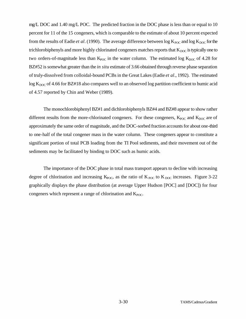
3-30 TAMS/Cadmus/Gradient
mg/L DOC and 1.40 mg/L POC. The predicted fraction in the DOC phase is less than or equal to 10
percent for 11 of the 15 congeners, which is comparable to the estimate of about 10 percent expected
from the results of Eadie et al. (1990). The average difference between log KPOC and log KDOC for the
trichlorobiphenyls and more highly chlorinated congeners matches reports that KDOC is typically one to
two orders-of-magnitude less than KPOC in the water column. The estimated log KDOC of 4.28 for
BZ#52 is somewhat greater than the in situ estimate of 3.66 obtained through reverse phase separation
of truly-dissolved from colloidal-bound PCBs in the Great Lakes (Eadie et al., 1992). The estimated
log KDOC of 4.66 for BZ#18 also compares well to an observed log partition coefficient to humic acid
of 4.57 reported by Chin and Weber (1989).
The monochlorobiphenyl BZ#1 and dichlorobiphenyls BZ#4 and BZ#8 appear to show rather
different results from the more-chlorinated congeners. For these congeners, KPOC and KDOC are of
approximately the same order of magnitude, and the DOC-sorbed fraction accounts for about one-third
to one-half of the total congener mass in the water column. These congeners appear to constitute a
significant portion of total PCB loading from the TI Pool sediments, and their movement out of the
sediments may be facilitated by binding to DOC such as humic acids.
The importance of the DOC phase in total mass transport appears to decline with increasing
degree of chlorination and increasing KPOC, as the ratio of K POC to K DOC increases. Figure 3-22
graphically displays the phase distribution (at average Upper Hudson [POC] and [DOC]) for four
congeners which represent a range of chlorination and KPOC.
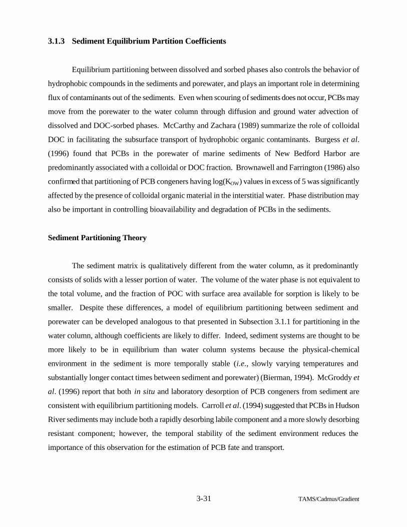
3-31 TAMS/Cadmus/Gradient
3.1.3 Sediment Equilibrium Partition Coefficients
Equilibrium partitioning between dissolved and sorbed phases also controls the behavior of
hydrophobic compounds in the sediments and porewater, and plays an important role in determining
flux of contaminants out of the sediments. Even when scouring of sediments does not occur, PCBs may
move from the porewater to the water column through diffusion and ground water advection of
dissolved and DOC-sorbed phases. McCarthy and Zachara (1989) summarize the role of colloidal
DOC in facilitating the subsurface transport of hydrophobic organic contaminants. Burgess et al.
(1996) found that PCBs in the porewater of marine sediments of New Bedford Harbor are
predominantly associated with a colloidal or DOC fraction. Brownawell and Farrington (1986) also
confirmed that partitioning of PCB congeners having log(KOW) values in excess of 5 was significantly
affected by the presence of colloidal organic material in the interstitial water. Phase distribution may
also be important in controlling bioavailability and degradation of PCBs in the sediments.
Sediment Partitioning Theory
The sediment matrix is qualitatively different from the water column, as it predominantly
consists of solids with a lesser portion of water. The volume of the water phase is not equivalent to
the total volume, and the fraction of POC with surface area available for sorption is likely to be
smaller. Despite these differences, a model of equilibrium partitioning between sediment and
porewater can be developed analogous to that presented in Subsection 3.1.1 for partitioning in the
water column, although coefficients are likely to differ. Indeed, sediment systems are thought to be
more likely to be in equilibrium than water column systems because the physical-chemical
environment in the sediment is more temporally stable (i.e., slowly varying temperatures and
substantially longer contact times between sediment and porewater) (Bierman, 1994). McGroddy et
al. (1996) report that both in situ and laboratory desorption of PCB congeners from sediment are
consistent with equilibrium partitioning models. Carroll et al. (1994) suggested that PCBs in Hudson
River sediments may include both a rapidly desorbing labile component and a more slowly desorbing
resistant component; however, the temporal stability of the sediment environment reduces the
importance of this observation for the estimation of PCB fate and transport.
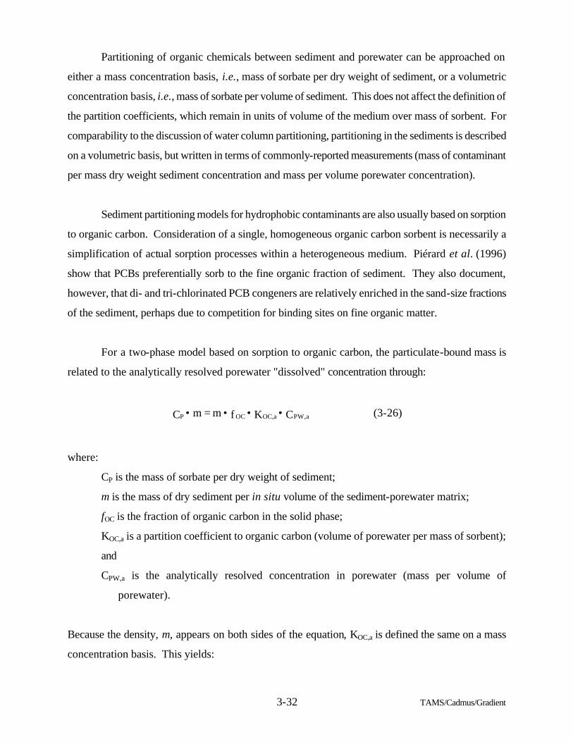
3-32 TAMS/Cadmus/Gradient
Partitioning of organic chemicals between sediment and porewater can be approached on
either a mass concentration basis, i.e., mass of sorbate per dry weight of sediment, or a volumetric
concentration basis, i.e., mass of sorbate per volume of sediment. This does not affect the definition of
the partition coefficients, which remain in units of volume of the medium over mass of sorbent. For
comparability to the discussion of water column partitioning, partitioning in the sediments is described
on a volumetric basis, but written in terms of commonly-reported measurements (mass of contaminant
per mass dry weight sediment concentration and mass per volume porewater concentration).
Sediment partitioning models for hydrophobic contaminants are also usually based on sorption
to organic carbon. Consideration of a single, homogeneous organic carbon sorbent is necessarily a
simplification of actual sorption processes within a heterogeneous medium. Piérard et al. (1996)
show that PCBs preferentially sorb to the fine organic fraction of sediment. They also document,
however, that di- and tri-chlorinated PCB congeners are relatively enriched in the sand-size fractions
of the sediment, perhaps due to competition for binding sites on fine organic matter.
For a two-phase model based on sorption to organic carbon, the particulate-bound mass is
related to the analytically resolved porewater "dissolved" concentration through:
where:
CP is the mass of sorbate per dry weight of sediment;
m is the mass of dry sediment per in situ volume of the sediment-porewater matrix;
fOC is the fraction of organic carbon in the solid phase;
KOC,a is a partition coefficient to organic carbon (volume of porewater per mass of sorbent);
and
CPW,a is the analytically resolved concentration in porewater (mass per volume of
porewater).
Because the density, m, appears on both sides of the equation, KOC,a is defined the same on a mass
concentration basis. This yields:
C K f m = m C PW,aOC,aOCP •••• (3-26)
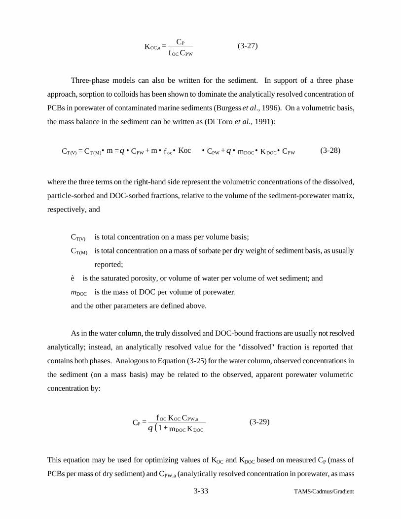
3-33 TAMS/Cadmus/Gradient
Three-phase models can also be written for the sediment. In support of a three phase
approach, sorption to colloids has been shown to dominate the analytically resolved concentration of
PCBs in porewater of contaminated marine sediments (Burgess et al., 1996). On a volumetric basis,
the mass balance in the sediment can be written as (Di Toro et al., 1991):
where the three terms on the right-hand side represent the volumetric concentrations of the dissolved,
particle-sorbed and DOC-sorbed fractions, relative to the volume of the sediment-porewater matrix,
respectively, and
CT(V) is total concentration on a mass per volume basis;
CT(M) is total concentration on a mass of sorbate per dry weight of sediment basis, as usually
reported;
è is the saturated porosity, or volume of water per volume of wet sediment; and
mDOC is the mass of DOC per volume of porewater.
and the other parameters are defined above.
As in the water column, the truly dissolved and DOC-bound fractions are usually not resolved
analytically; instead, an analytically resolved value for the "dissolved" fraction is reported that
contains both phases. Analogous to Equation (3-25) for the water column, observed concentrations in
the sediment (on a mass basis) may be related to the observed, apparent porewater volumetric
concentration by:
This equation may be used for optimizing values of KOC and KDOC based on measured CP (mass of
PCBs per mass of dry sediment) and CPW,a (analytically resolved concentration in porewater, as mass
C f
C = KPWOC
POC,a (3-27)
C K m + C Kocf m + C = m C = C PWDOCDOCPWocPW(M) T(V) T •••••••• θθ (3-28)
( )K m + 1 C K f = C
DOCDOC
PW,aOCOCP θ
(3-29)
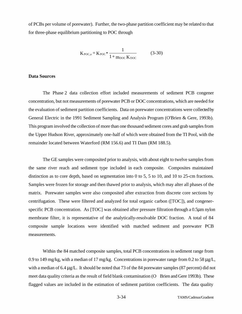
3-34 TAMS/Cadmus/Gradient
of PCBs per volume of porewater). Further, the two-phase partition coefficient may be related to that
for three-phase equilibrium partitioning to POC through
Data Sources
The Phase 2 data collection effort included measurements of sediment PCB congener
concentration, but not measurements of porewater PCB or DOC concentrations, which are needed for
the evaluation of sediment partition coefficients. Data on porewater concentrations were collected by
General Electric in the 1991 Sediment Sampling and Analysis Program (O'Brien & Gere, 1993b).
This program involved the collection of more than one thousand sediment cores and grab samples from
the Upper Hudson River, approximately one-half of which were obtained from the TI Pool, with the
remainder located between Waterford (RM 156.6) and TI Dam (RM 188.5).
The GE samples were composited prior to analysis, with about eight to twelve samples from
the same river reach and sediment type included in each composite. Composites maintained
distinction as to core depth, based on segmentation into 0 to 5, 5 to 10, and 10 to 25-cm fractions.
Samples were frozen for storage and then thawed prior to analysis, which may alter all phases of the
matrix. Porewater samples were also composited after extraction from discrete core sections by
centrifugation. These were filtered and analyzed for total organic carbon ([TOC]), and congener-
specific PCB concentration. As [TOC] was obtained after pressure filtration through a 0.5µm nylon
membrane filter, it is representative of the analytically-resolvable DOC fraction. A total of 84
composite sample locations were identified with matched sediment and porewater PCB
measurements.
Within the 84 matched composite samples, total PCB concentrations in sediment range from
0.9 to 149 mg/kg, with a median of 17 mg/kg. Concentrations in porewater range from 0.2 to 58 µg/L,
with a median of 6.4 µg/L. It should be noted that 73 of the 84 porewater samples (87 percent) did not
meet data quality criteria as the result of field blank contamination (O�Brien and Gere 1993b). These
flagged values are included in the estimation of sediment partition coefficients. The data quality
K m + 1
1 K = K
DOCDOCPOCa POC, • (3-30)
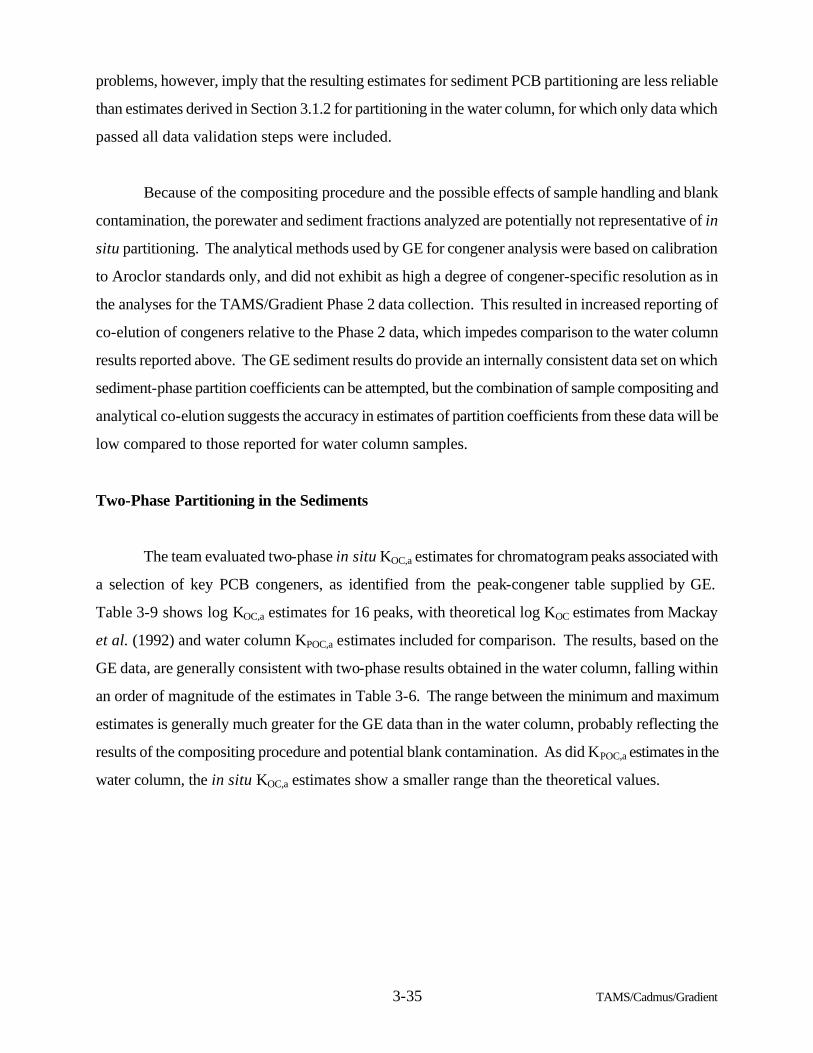
3-35 TAMS/Cadmus/Gradient
problems, however, imply that the resulting estimates for sediment PCB partitioning are less reliable
than estimates derived in Section 3.1.2 for partitioning in the water column, for which only data which
passed all data validation steps were included.
Because of the compositing procedure and the possible effects of sample handling and blank
contamination, the porewater and sediment fractions analyzed are potentially not representative of in
situ partitioning. The analytical methods used by GE for congener analysis were based on calibration
to Aroclor standards only, and did not exhibit as high a degree of congener-specific resolution as in
the analyses for the TAMS/Gradient Phase 2 data collection. This resulted in increased reporting of
co-elution of congeners relative to the Phase 2 data, which impedes comparison to the water column
results reported above. The GE sediment results do provide an internally consistent data set on which
sediment-phase partition coefficients can be attempted, but the combination of sample compositing and
analytical co-elution suggests the accuracy in estimates of partition coefficients from these data will be
low compared to those reported for water column samples.
Two-Phase Partitioning in the Sediments
The team evaluated two-phase in situ KOC,a estimates for chromatogram peaks associated with
a selection of key PCB congeners, as identified from the peak-congener table supplied by GE.
Table 3-9 shows log KOC,a estimates for 16 peaks, with theoretical log KOC estimates from Mackay
et al. (1992) and water column KPOC,a estimates included for comparison. The results, based on the
GE data, are generally consistent with two-phase results obtained in the water column, falling within
an order of magnitude of the estimates in Table 3-6. The range between the minimum and maximum
estimates is generally much greater for the GE data than in the water column, probably reflecting the
results of the compositing procedure and potential blank contamination. As did KPOC,a estimates in the
water column, the in situ KOC,a estimates show a smaller range than the theoretical values.
3-36 TAMS/Cadmus/Gradient
Three-Phase Partitioning in the Sediments
Three-phase partition coefficients were estimated using the GE sediment�porewater data. For
several congeners, three-phase estimates did not converge through direct optimization, or yielded
estimates which did not appear to reproduce observed total porewater concentrations well. For some
congeners, a few anomalous data points appeared to bias the optimization, and estimates were re-
calculated with deletion of up to three such outliers. For three congeners, an alternative procedure
was required to obtain estimates which approximated the observed ratio of CPW,a to CP. In general, the
net effects of KDOC and KOC, determining the total concentration measured in porewater, should be
more strongly determined by the data than either individual partition coefficient. Accordingly, a
procedure was adopted which assumed that KOC,a could be estimated more reliably than three-phase
coefficients, and the three-phase coefficients can therefore be determined conditional on the two-phase
estimate of KOC,a. Based on Equation (3-30), the equilibrium estimate of log(KDOC) should be
approximately equal to
Therefore, a conditional estimate of KDOC, given an estimate of KOC, can be made by using the two-
phase estimate of KOC,a and averaging over all samples. With the relationship between KDOC and KOC
determined by Equation (3-31), optimization is applied to KOC only. This procedure successfully
reproduces the median ratio of total porewater concentration to particulate concentration for a
congener, but is less preferable than full optimization because it assumes that the two-phase estimate
of KOC,a is known without error.
Resulting partition coefficient estimates are summarized in Table 3-10a. Because PCBs are
strongly hydrophobic, most of the total mass of each congener is expected to be sorbed to particulate
matter. The implications of the estimated partition coefficients are summarized in Table 3-10b by
showing the predicted distribution of concentration in interstitial water (in ng/L) in response to a unit
total sediment concentration of 1 mg/kg. Table 3-10b also shows the median observed ratio between
total porewater concentration (ng/L) and sediment concentration (mg/kg dry weight) in the GE
samples. For comparison, the tables show results summarized by homologue group in New Bedford
) m K( log - )K - K( log = )K( log DOC,a OC,a OCOCDOC • (3-31)
3-37 TAMS/Cadmus/Gradient
Harbor sediments by Burgess et al. (1996), and partitioning in porewater which would be implied by
application of the three-phase partition coefficients obtained in the water column of the Hudson River.
The analysis of partitioning in the sediments should be used with caution, because the method
of compositing and sample handling together with reported sample contamination suggests the
porewater samples may not be representative of in situ conditions in the sediment. The problem of
potential readjustment of phase distribution after sampling is exacerbated wherever PCB
concentrations or [DOC] differ significantly among the sub-samples in a composite. Indeed, the
research of Burgess et al. (1996) suggests that natural colloidal porewater systems may often not
achieve equilibrium because there is insufficient time for contaminants with large KOW values to fully
equilibrate with interstitial water colloids before the colloids are altered in some way (e.g., by
aggregation and settling) or transported from the sediments. In addition, the mass of PCBs is
predominantly in the particulate-sorbed phase, with at least 99.9 percent of the total mass of all
congeners in this phase. This means that the equation used for optimizations is very sensitive to small
errors in fOC and mDOC.
The resulting estimates of porewater concentrations relative to total sediment concentrations in
the Hudson differ from those implied by three-phase partition coefficients estimated by Burgess et al.
(1996) for New Bedford Harbor sediments. This work suggested that KDOC is close in magnitude to
KOC, and approximately 80 percent of the porewater fraction of tri- and higher-chlorinated PCB
congeners is associated with the colloidal fraction. Partition coefficients (KOC, KDOC) reported by
Burgess et al., however, were obtained for a very different geochemical environment of a saline
marine sediment, and would appear to over-predict the total porewater concentrations reported by GE
in sediments of the freshwater portions of the Hudson. In contrast, applying the three-phase partition
coefficients obtained for the water column to the sediment generally under-predicts GE�s reported
total porewater concentrations.
Both the analysis of data for Hudson River sediments and Burgess et al.�s results for New
Bedford Harbor suggest that DOC-bound PCBs may constitute a significant fraction of the PCB
concentrations in porewater. Further, elevated concentrations of mono- and dichlorobiphenyls in
porewater relative to concentrations of more highly-chlorinated congeners. This phenomenon may
facilitate transport of these congeners from the sediment to the water column.
3-38 TAMS/Cadmus/Gradient
3.1.4 Summary
In this section, two- and three-phase sediment-water partition coefficients were developed
based on Phase 2 water column transect data. These coefficients could only be established for those
congeners which had measurable concentrations in both the �dissolved� and suspended matter
samples. Coefficients were calculated for a total of 64 congeners. The two-phase partition
coefficients had a more limited range than those predicted in the literature based on octanol-water
partitioning. The reason for this is unclear but may be due in part to the inclusion of the DOC-bound
fraction in the measured �dissolved� fraction. The DOC-bound fraction is relatively more important
to the congeners with lower partition coefficients and lower molecular weights, as demonstrated by
the three-phase partition coefficient analysis also performed here.
Two-phase partition coefficients were shown to be consistent within a water column transect
for the stations at TI Dam and downstream. The stations upstream of the TI Dam, particularly Station
4 at Rogers Island, were shown to exhibit substantively different dissolved to suspended matter phase
partitioning, suggesting non-equilibrium conditions at these stations. The use of a temperature
correction term with the two-phase partition coefficient for particulate organic carbon (KPOC,a) was
shown to be the best predictor of in situ partitioning with a mean difference of 43 percent for all
stations and a difference of only 33 percent for stations downstream of TI Dam. Thus, with accurate
measurements of in situ temperature, total suspended solids, and particulate organic carbon, it is
possible to predict the phase distribution of PCB congeners to within about 33 percent for the
freshwater Hudson below the TI Dam.
Three-phase partition coefficients for the water column were calculated from the Phase 2 data
as well. Based on these coefficients, the distributions of several congeners among truly dissolved,
DOC-bound, and suspended matter bound phases were examined. The results demonstrated that the
DOC-bound fraction may be as large as the truly dissolved fraction for the lightest congeners. The
analysis also showed that the truly dissolved and DOC-bound fractions decrease in importance as
congener molecular weight (i.e., degree of chlorination) increases.

3-39 TAMS/Cadmus/Gradient
Composite sample porewater data collected by GE were used to evaluate partitioning between
sediment and porewater, and yielded two- phase partition coefficients that were generally consistent
with the Phase 2 program water column results. Analysis of three-phase partitioning in sediment
suggests that the DOC-bound phase may constitute a significant fraction of the total porewater
concentration for most congeners. Further, because of their lower partition coefficients (KOC and
KDOC), concentration of mono- and dichlorobiphenyls is enhanced in porewater relative to more highly
chlorinated congeners, which may facilitate loading of these congeners from the sediment to the water
column.
3.2 Water Column Mass Loading
Investigation of the transport of PCBs through the Hudson River by a mass loading analysis
allows for the identification of the relative importance of the various PCB sources and sinks. This
understanding of PCB mass transport is of critical importance in assessing the impact of the Upper
Hudson River sources on the freshwater Lower Hudson River and in assessing the feasibility of
remedial alternatives for mitigating the contamination located in the Upper River sediment.
In this mass loading analysis, water column samples, collected as part of the Phase 2
investigation, are evaluated in terms of PCB mass loading on a homologue basis. As part of this
evaluation, several mechanisms, including porewater diffusion/advection and sediment resuspension,
are considered for their potential impacts on the water column PCB inventory. In addition, the
seasonal variability of PCB fate and transport in the Upper River is examined. In this section,
emphasis is placed on the understanding of PCB loads on a total PCB and homologue basis.
Subsequent sections will examine PCB loads using congener-specific information.
3.2.1 Phase 2 Water and Sediment Characterization
In order to monitor the transport of PCBs in the Upper Hudson River, two water sampling
techniques and a sediment sampling technique were applied as part of the Phase 2 investigation. Each
of these sampling methods provides unique insight into the various PCB sources and sinks located in
the Upper River.
3-40 TAMS/Cadmus/Gradient
The first water column sampling scheme was the transect sampling program. This program
was designed to provide a measure of the instantaneous water column conditions. Samples were
collected in a timed sequence beginning at Fenimore Bridge (RM 197.2) so as to consistently sample
the same parcel of water as the parcel traveled downstream to Waterford (RM 156.5). These samples
were filtered within four hours of collection using 0.7µm glass fiber filters to separate the dissolved
phase and suspended matter-borne PCB fractions. The relative distribution of PCBs in the dissolved
and suspended-matter phases is important in that it provides information on the nature of PCB sources
to the water column as well as on those mechanisms by which the water column inventory is altered.
The second water column sampling scheme was the flow-averaged sampling program. This
program provided a measure of relatively long-term (15-day) mean water column conditions. As part
of the flow-averaged water sampling program, samples were collected on alternate days over a 15-
day period, composited on the basis of river flow, and filtered to separate the dissolved-phase and
suspended matter-borne PCB fractions. However, because the holding times varied among the
individual pre-composited samples, the measured partitioning of PCBs between the suspended matter
and the dissolved phase for the composited samples is considered less reliable than that measured in
the transect study. Therefore, only total PCB concentrations, i.e., the sum of the suspended matter
fraction PCB concentration and the dissolved-fraction PCB concentration, of the composited samples
are evaluated in this mass loading analysis.
While the flow-averaged sampling analysis does not provide information on the relative
distribution of PCBs in the dissolved and suspended-matter phases, it is an important tool in
understanding the fate and transport of PCBs in the Upper River. Specifically, it provides a basis by
which to assess whether or not the instantaneous measurements obtained in the transect study are
representative of longer-term fate and transport trends.
The sediment investigation entitled the �high -resolution sediment coring study� was
developed as part of the Phase 2 investigation to gain insight into long-term, i.e., historical, PCB input,
transport, and dechlorination/degradation in the Hudson River. This investigation is discussed in
detail in Subsection 2.1.2 of the Final Phase 2 Work Plan and Sampling Plan (USEPA, 1992b).
The coring study is an essential component of the mass balance analysis because it provides
information on the nature of the PCBs entering the water column via resuspension. In addition, by
3-41 TAMS/Cadmus/Gradient
assuming that sediment porewater is in equilibrium with sediments at 0 to 8 cm (0 to 3 in.), it provides
information on the nature of the PCBs which may enter the river via porewater diffusion and
advection.
3.2.2 Flow Estimation
In a mass loading analysis, it is of critical importance to know the flow rate associated with
each sample collected so that the corresponding PCB loading can be calculated. Flow data collected
by the USGS at RM 194.5 (Fort Edward) are available for the time period corresponding to the Phase
2 sampling program (USGS, 1993a). However, direct measurements of flow normally collected by
the USGS at the Stillwater and Waterford sampling points were not available due to construction
activities at the Stillwater Dam and at Lock 1. In addition, indirect estimates of flow by the USGS
were not available at the initial time of preparation of this analysis. As a result, flow estimates for
these stations were made based on the reported Fort Edward flow and daily staff gauge readings
collected by the New York State Thruway Authority, Office of Canals (1993, 1994a, 1994b) (formerly
administered by NYSDOT). Because the flow estimates developed here are based on in-river staff
gauges, they are considered to be as good or better than the indirect estimates made by the USGS and
thus were not replaced when the USGS data became available.
In order to estimate flow conditions during the Phase 2 sampling period, several least-squares
fit models were developed which relate mean daily flow to the staff-gauge heights. Staff gauges,
which are located immediately upstream and downstream of each of the locks on the Champlain Canal
(see Plate 3-1), are maintained by the Thruway Authority for the purpose of monitoring water levels in
the barge canal with respect to the New York State Barge Canal Datum.
These models are accurate in that they provide estimates of flow at Stillwater with a
prediction uncertainty of roughly "15 percent under low-flow conditions and "10 percent under high-
flow conditions, based on an analysis of 10 years of USGS flow and staff gauge data. Similarly, flow
at Waterford can be estimated with a prediction uncertainty of roughly "25 percent under low-flow
conditions and "15 percent under high-flow conditions.
3-42 TAMS/Cadmus/Gradient
Model Development
As an initial step in the development of the models, the staff-gauge data were screened to
remove outliers, i.e., gauge readings which were significantly different from the trend of the data set.
Further, gauge readings taken between December 15 and March 15 of each year were excluded to
eliminate the impact of inaccuracies caused by ice formation on the Hudson River.
Flow models were developed using various combinations of daily measurement data from
several staff gauges and USGS-recorded Fort Edward flow as parameters. In addition, to improve the
quality of predictions under low-flow conditions, i.e., a Fort Edward flow less than or equal to 8,000
cfs, a second set of models was developed to better account for variability observed in the staff-gauge
data under these conditions. These models were calibrated using Stillwater and Waterford flow data
collected by the USGS between 1983 and 1992 (USGS, 1993b).
The rationale for using the data from several gauges to predict flow is that all of the gauges are
hydraulically linked together, i.e., an increase in flow measured at one gauge is observed to some
degree at each of the downstream gauges. Assuming that errors associated with the gauge readings are
random and not systematic in nature, flow prediction using the data from several gauges improves the
predictive ability of the model by minimizing the significance of the error associated with any
particular gauge reading. In addition, because the availability of gauge data varies from day to day
during Water Year 1993 (i.e., each gauge was not read every day), using the data from several gauges
to predict flow provided the flexibility to develop models to match the various combinations of
available data. Note that USGS data are referenced here according to the USGS-defined water year
which extends from October 1 to September 30 and is labeled by the latter year (e.g., water year 1993
extends from October 1, 1992 to September 30, 1993).
As part of model development, the flow data available for the 1983 to 1992 period of record
were evaluated to determine the potential importance of response time at downstream stations with
respect to changes in the magnitude of the flow measured at Fort Edward. From this evaluation, it was
determined that the Hudson River and its associated watershed largely behave as a single unit between
Fort Edward and Waterford. That is, while flow is a function of several factors including upstream
input, tributary input and localized precipitation events, flow changes observed at downstream
3-43 TAMS/Cadmus/Gradient
locations are generally coincident with flow changes observed at Fort Edward. This is evidenced by
the nearly identical tracking of slope changes in the hydrographs for each of the stations (see Figure 3-
23).
During periods of low flow, however, there does appear to be a time lag of, at most, one day
between the hydrograph slope change measured at Fort Edward and that measured at Waterford. To
account for the potential predictive significance of this lag, contemporaneous Fort Edward flow as
well as Fort Edward flow with a one-day lag were considered as parameters in the model
development for downstream stations. Using a step-wise regressing method, the more statistically
significant, if either one was significant, was included in the least-squares models.
It is important to note that exceptions to the singular watershed response also occur on
occasion when, for example, there is a localized precipitation event that does not occur over the entire
watershed. This lack of singular watershed response was an important consideration for flows
predicted between March 27 and April 5; during this period, the lower portion of the Upper River
drainage basin was beginning its spring flood while the upper portion of the Hudson River drainage
basin had not yet begun to thaw. In order to minimize the impact of the disproportionate watershed
response, gauge-only models utilizing only nearby staff gauges were developed to predict Stillwater
and Waterford flows during this time period. No Upper River gauge data or Fort Edward flow data
were included as predictive parameters in these models to avoid under-estimating the Stillwater and
Waterford flows as a result of the disproportionately low upstream response.
Flow Prediction Results
The flow prediction model parameters and the corresponding Stillwater and Waterford flows
calculated for the Phase 2 period of study (January through September, 1993) are listed in Tables 3-11
and 3-12, respectively. The predicted flows were calculated using the best model appropriate for the
staff-gauge data available. When the available gauge data were such that flow could be calculated
using more than one of the models developed, flow was calculated using the model with the lowest
prediction error. However, as was noted previously, Stillwater and Waterford flows for the March
27 to April 5 time period were predicted using single-gauge models even though sufficient gauge data
were available to allow for the use of better models, i.e., models with lower prediction errors.
3-44 TAMS/Cadmus/Gradient
In addition, for several isolated days during Water Year 1993, the available gauge data are not
sufficient for flow calculation. Flow estimates for these days were interpolated using temporally
adjacent predicted flows. It is important to note that Stillwater and Waterford flows were predicted
for January 1 through March 15, 1993 based on available flow and staff gauge data even though the
corresponding staff-gauge data for this time period were excluded in model calibration due to
potential inaccuracies noted previously.
Flow Prediction Uncertainty
In order to use the estimated flows predicted with the flow models appropriately, it is
important to quantify the error associated with each of the estimated flows. Interpretation of the
prediction errors presented some statistical problems due to the autocorrelation between the
"independent" variables. Specifically, while the correlation between independent variables does not
diminish the ability of the models to predict flow, it does distort the estimates of model error, i.e., the
quality of fit estimate, r2, and the root mean square error. However, because the gauge and flow data
sets are large, it was possible to assess the prediction error directly by evaluating the distribution of
the percent residual errors, i.e., the distribution of the percent differences between the predicted flows
and the measured flows was evaluated for each of the models for each of the flow regimes. A
summary of this analysis, which indicates the bounds of the central 95th percentile associated with the
distribution of the percent residual errors for each of the models, is presented in Tables 3-13 and 3-
14.
As is evident in Tables 3-13 and 3-14, model prediction error is highly dependent on the flow
regime as well as the model used. For each of the models generated, the prediction error, as
represented by the bounds of the central 95 percent quantile, is much greater for low-flow conditions
and decreases as the flow increases. In short, the higher the flow, the more accurately it can be
predicted. An example of the dependence of prediction error on flow regime is illustrated in the plot
of percent residual error vs. Stillwater flow for low-flow Model C (see Figure 3-24).
In addition to evaluating the prediction error associated with each of the models developed, it
is important to evaluate whether or not any systematic errors are introduced by using different models
3-45 TAMS/Cadmus/Gradient
as dictated by the available data and the flow conditions. As illustrated in Figure 3-25, the flows
predicted using the low-flow Stillwater models are generally within 15 percent of each other, which is
comparable to the range of Stillwater low-flow model prediction errors presented in Table 3-13.
Similarly, as illustrated in Figure 3-26, the flows predicted using the high-flow Stillwater models are
all generally within 10 percent of each other, which is comparable to the Stillwater high-flow model
prediction errors. In addition, during the transition periods between high- and low-flow conditions,
i.e., late March and early May, flows predicted using the low-flow Stillwater models compare well
with flows predicted using the high-flow Stillwater models (see Figure 3-27). Similar results were
obtained for the Waterford models, as indicated by a comparison of Figures 3-28, 3-29, and 3-30 with
the prediction errors presented in Table 3-14. Thus, it appears that no additional error is introduced
by using different models to predict flow for Water Year 1993.
3.2.3 Fate Mechanisms
On the most basic level, the water column PCB inventory at any location is defined by the
integrated sum of all upstream sources and losses, both external and internal to the river. Regardless
of its pathway, once introduced to the river by external sources PCBs are then subject to the
geochemical process internal to the river. Excluding the external load processes, there are several
mechanisms by which PCBs can be introduced to and lost from the water column. The primary
mechanisms examined in this mass balance analysis include:
• Simple advection
• Sediment resuspension and settling of suspended solids
• Porewater diffusion/advection
• Gas exchange
• Destruction in the water column
As indicated in the following descriptions of the PCB flux mechanisms, each mechanism which
is significant within a particular river segment will alter the congener distribution in a unique manner
consistent with the appropriate partitioning characteristics or source(s) associated with the
mechanism. Therefore, the relative importance of each of these mechanisms can be determined by
evaluating the change in water column homologue distribution across the reach.
3-46 TAMS/Cadmus/Gradient
Water Column Impacts
For each of the water column PCB source and loss mechanisms, the manner in which it impacts
the water column is dependent on the relative partitioning of the PCBs between the dissolved and
suspended-matter phases. Specifically, PCBs are hydrophobic and tend to bind preferentially to
organic carbon present in suspended solids in the water column, dissolved in the water column, or in
the sediments on the river bottom. In the subsequent discussions, suspended and dissolved phase
PCBs will be defined by the operational definitions (i.e., suspended phase PCBs are those PCBs
retained by a 0.7 µm glass fiber filter; dissolved phase PCBs are those which pass through the filter,
encompassing both truly dissolved and DOC-bound PCBs). The relative distribution between the
dissolved and suspended-matter phases is dependent on the mass-based, congener-specific partition
coefficient, the determination of which is discussed in detail in Section 3.1. In general, the more-
chlorinated PCB congeners are more hydrophobic than the less-chlorinated congeners, and, therefore,
tend to bind more tightly to suspended matter. This is a particularly important phenomenon since it
provides a tool to differentiate among the PCB gain and loss mechanisms.
Simple Advection
The water column PCB inventory of a given river segment can be increased as a result of
simple advection of PCBs from upstream and local tributary contributions. These increases, however,
must be consistent with the homologue distributions of the sources. Similarly, PCBs can be lost from
the water column through various means, such as advective transport downstream.
It is important to note that if an upstream input has not reached equilibrium conditions, the
increase in water column PCB loading measured in the adjacent downstream river segment may be
superimposed on re-partitioning between the dissolved and suspended-matter phases. In addition, re-
partitioning may occur upon addition of clean tributary input, i.e., input not contaminated with PCBs,
resulting in changing the concentration and nature of the suspended solids in the water column.
However, under the flow and suspended solids loading conditions measured during the Phase 2
investigation, the theoretical magnitude of this latter re-partitioning phenomenon appears to be largely
within the uncertainty of the calculated partition coefficients (i.e., the variability of partition
coefficients downstream of the TI Dam does not appear systematic, see Section 3.1). Thus, its relative
3-47 TAMS/Cadmus/Gradient
importance cannot be independently determined. Because the homologue distributions between
suspended and dissolved phases associated with the mainstem water column PCB loads were
generally unaffected upon addition of clean tributary input, this latter re-partitioning phenomenon does
not appear to be important under the conditions measured during the Phase 2 investigation.
When advective transport is considered on a whole water basis, thus accounting for re-
partitioning of the congeners, the total PCB loading from the upstream input should be conserved
assuming no additional PCB input. In contrast, the relative distributions of the congeners in the
dissolved and suspended-matter phases may change dependent upon the proximity of in situ conditions
to equilibrium.
Resuspension and Settling
PCBs can be lost from or added to the water column through settling of suspended solids and
resuspension of sediment. The distribution of homologues lost from the water column through settling
of suspended solids will reflect the homologue distribution associated with the suspended solids.
Similarly, PCBs introduced through resuspension will reflect the homologue distribution of the
surficial sediments. Either case can potentially change the homologue pattern in the water column.
Because the more-chlorinated, hydrophobic congeners tend to bind more aggressively to the
sediment than the less-chlorinated congeners, the settling of suspended matter tends to preferentially
remove the more-chlorinated congeners from the water column. Conversely, dependent upon the
nature of the sediments, resuspension of sediment may or may not increase the content of the more-
chlorinated congeners in the water column. If largely unmodified PCBs are at the surface,
resuspension will tend to increase or maintain the fraction of more chlorinated congeners, depending
upon the similarity of the sediments to the existing water column inventory. Alternatively, if sediments
containing partly dechlorinated PCBs are resuspended (perhaps via scour of older, altered sediments),
the homologue pattern will shift toward the less-chlorinated congeners. Dechlorination in the
sediments and the likely nature of resuspended sediments are discussed in detail in Sections 4.3 and
4.4.
It is useful at this point in the discussion to differentiate between net and gross contributions to
the water column load. As part of the Phase 2 program, PCB measurements permit the calculation of
3-48 TAMS/Cadmus/Gradient
the net PCB load gain or loss between any two sampling points. This is accomplished by simply
subtracting the PCB load at the downstream station from that of the upstream station. In this fashion,
changes in the total water column PCB load are attributed to various portions of the river. However,
the measurement of the net loss or gain does not address the gross exchange processes. It is possible,
and even likely in some cases, that gross rates of exchange between sediment and water may dwarf the
net or total PCB transport downstream. In this manner, upstream loads are effectively stored and
replaced with PCBs generated within a given segment of the river. Sediment resuspension and settling
is generally considered the principal means of accomplishing such an exchange, although sediment
porewater transport may be involved as well. In this fashion, even when loads are constant, the water
column inventory can be completely replaced. Unfortunately, it is not easy to establish the gross rates
of settling and resuspension. The use of the homologue and congener patterns can provide some clues
as to the actual replacement rate but generally do not yield them explicitly. In this analysis, it has been
typically more successful to use these patterns to establish the character of the sediments involved in
sediment-water interactions rather than the gross rates of exchange.
Porewater Diffusion/Advection
The flux of PCBs from the sediment porewater must also be considered as a potential PCB
source to the water column. Capel and Eisenreich (1990) report PCB concentrations in porewater
samples from the Great Lakes to be anywhere from 10 to 500 times greater than the corresponding
water column concentrations. These elevated concentrations suggest that PCBs may exhibit greater
mobility and biological availability within the sediment and are, therefore, a viable source of PCBs to
the overlying water column. The study by Capel and Eisenreich also suggests that the ratio between
the PCB sediment concentration and the PCB porewater concentration is a function of the
dissolved/colloidal organic carbon (DOC) in the porewater. No porewater measurements were made
during the Phase 2 sampling effort. However, an estimate of porewater DOC is available from the
sediment sampling program conducted by GE in 1991 (O'Brien & Gere, 1993b). This program
yielded composited porewater DOC levels with a median level of 37 mg/L and a range of 10 to 212
mg/L. The median level is seven times greater than the median Phase 2 water column level of 5 mg/L.
GE also analyzed these composited porewater samples of PCBs although the compositing and other
sample processing techniques may have seriously affected the accuracy of the results. These data are
mentioned here only for comparison purposes due to the great concern over sample accuracy and
representativeness. As noted in Section 3.1, GE porewater results yielded a median composited total
3-49 TAMS/Cadmus/Gradient
PCB concentration of 6,430 ng/L with a range of 230 to 57,700 ng/L. These porewater samples were
obtained from composited sediments in the range of 920 (0.92 ppm) to 149,000 µg/kg (149 ppm) with a
median value of 17,000 µg/kg (17 ppm).
It is difficult to estimate the distribution of PCBs entering the water column as a result of
porewater diffusion and advection. As noted in Section 3.1, conditions affecting porewater
equilibrium may be quite different from those governing the water column. Water to sediment ratios
are vastly different as are the DOC levels as noted above. However, lacking other data, it may be
possible to characterize the porewater congener distribution using the partition coefficients determined
for the water column dissolved-phase and suspended matter-phase distributions without correction for
porewater DOC. An alternative means to describe the porewater PCB distribution is to use the three-
phase equilibrium coefficients derived from the Phase 2 and GE data sets. As discussed in Section
3.1, in both instances the data are of limited usefulness in this regard. The Phase 2 have low but
consistent DOC values, thus making the estimation of the DOC dependence difficult. The GE data
were subject to some questionable sample handling practices and exhibit a large degree of variability
in their porewater to sediment PCB concentration ratios. It is unknown whether the variability is the
result of the handling practices. While both data sets show substantive variability and differences in
the three-phase partition coefficients, they both indicate that the lighter congeners are preferentially
concentrated in the porewater relative to the heavier congeners. This is shown in detail for a suite of
14 congeners in Tables 3-10a and 3-10b. This is consistent with the lower two-phase partition
coefficients obtained for the Phase 2 data. Unlike the three-phase coefficient, the two-phase
coefficients are available for a large number of congeners and this can be used to calculate porewater
homologue distributions for comparison to sediment and surface water. These results are presented
later in this chapter.
Gas Exchange
Gas exchange is another mechanism by which the water column PCB inventory can be
modified. This transfer of PCBs across the air-water interface is dependent on the concentration
gradient across the interface and the liquid-phase to gas-phase transfer coefficient or piston velocity
which represents the rate of transfer. That is,
Flux = KL(CDissolved - Pcongener/Hcongener) (3-32)
3-50 TAMS/Cadmus/Gradient
where:
KL is the transfer coefficient or piston velocity in m/s;
CDissolved is the dissolved-phase congener concentration in moles/m3;
Pcongener is the congener partial pressure in the air overlying the river, in atmospheres; and
Hcongener is the congener-specific Henry's Law constant, in atm-m3/mole.
The Henry's Law constant is comparable to the previously defined water column suspended matter-
phase to dissolved-phase partition coefficient since it represents the ratio between the congener
vapor-phase concentration, or partial pressure, and its dissolved-phase concentration.
In order to understand how gas exchange potentially impacts the water column PCB inventory,
it is necessary to evaluate the dependence of the gas-exchange flux on congener-specific properties.
There are a variety of models which have been developed to predict the gas-transfer coefficient. The
two most common models are the stagnant film model and the surface renewal model. In the stagnant
film model, KL is a function of the transport of the PCBs by molecular diffusion across a stagnant
water film at the air-water interface while in the surface renewal model, the primary mechanism
controlling gas exchange is the replacement of the water at the interface with water from the bulk
solution.
Neither model can be easily applied since film thickness cannot be measured directly and the
rates of surface renewal are difficult to quantify (Liss, 1983). There are, however, several empirical
models which define KL in terms of measurable parameters. In these models, KL is controlled by shear
stress introduced either by wind or by water velocity and varies as a function of the square root of the
congener-specific molecular diffusivity. However, molecular diffusivity, as determined by Bopp
(1983) does not exhibit large variation across the PCB homologue groups. Therefore, because KL
varies as the square root of molecular diffusivity, it is, for all practical purposes, independent of
congener-specific properties.
In addition, for the range of concentrations measured during the Phase 2 sampling effort, the
gas-exchange flux is dependent on the dissolved-phase congener concentration and not the
concentration gradient across the air-water interface. That is, based on an estimate of the average
3-51 TAMS/Cadmus/Gradient
urban atmospheric congener partial pressure determined by Duinker and Bouchertall (1989) and the
Henry's Law constants obtained from several sources, including Warren et al. (1987), the
Pcongener/Hcongener ratio is roughly three orders of magnitude smaller than the measured dissolved-phase
PCB concentrations. Therefore, for all practical purposes, gas exchange is independent of the
Pcongener/Hcongener ratio.
These findings have important implications for the impact of gas exchange on the water column
PCB inventory. Specifically, as noted above, gas exchange is driven by the dissolved-phase congener
concentrations and is independent of congener-specific properties. Therefore, a loss in the water
column PCB inventory as a result of gas exchange should result in a decrease in the relative congener
concentrations that is consistent with the ratio of their dissolved-phase concentrations. In addition,
because the less-chlorinated congeners are proportionally more prevalent in the dissolved-phase than
the more-chlorinated congeners, they are more susceptible to gas exchange than the more-chlorinated
congeners. Thus, the net effect of loss due to gas exchange is preferential removal of the less-
hydrophobic, i.e., less-chlorinated congeners, from the water column, leaving behind a water column
inventory of relatively higher chlorinated congeners.
Destruction in the Water Column
Another mechanism by which the water column congener distribution can be altered is through
destruction within the water column itself. Work by Abramowicz (1990) and Bedard (1990) suggests
that some of the less-chlorinated congeners may be affected by these processes. However, these
processes are generally poorly understood and as such, the relative importance of water column
destruction, as compared to the other fate mechanisms, cannot be determined. Based on the detailed
analysis of the Phase 2 results, presented in Subsection 3.2.5, this fate mechanism is probably limited
to the warmer months of the year.
Seasonal Dependence of Fate Mechanisms
In addition to understanding the manner in which the various fate and transport mechanisms
impact the water column PCB inventory, it is important to consider the seasonal dependence of the
various mechanisms which alter the inventory.
3-52 TAMS/Cadmus/Gradient
Simple Advection
The seasonal dependence of simple advection of PCBs from upstream and local tributary
contributions is fairly straightforward: as flow increases, the loading rate increases. However,
because increases in flow effectively dilute the concentration of PCBs in the water column, the PCB
loading does not increase in direct proportion to the increase in flow.
Resuspension and Settling
Sediment resuspension is dependent on the flow rate and is, therefore, also seasonally
dependent. Specifically, resuspension results from shear stress imparted on the sediment particles by
the flow of the overlying water. As the flow rate increases, the stress applied to the sediment is
increased and particles deposited under lower-flow conditions may be resuspended. As the flow rate
increases, more and more particles are resuspended. Particles which can be resuspended by the
applied shear stress re-enter the water column. For fine-grained cohesive sediments (where the
highest PCB concentrations are found), no additional significant resuspension occurs until the shear
stress is further increased by an additional increase in flow rate. Therefore, extensive sediment scour
of cohesive sediments, typically associated with high-flow events such as the spring flood, occurs
during the period of increasing flows and is completed soon after peak flows occur. Further
significant resuspension occurs only with an additional increase in flow.
While cohesive sediments are scoured to their maximum possible depth relatively quickly in
response to peak flows, erosion of noncohesive sediments may continue for extended periods beyond
peak flows. Erosion of non-cohesive sediments will continue until the remaining particles in the
surficial sediments are too large to be eroded by the existing shear stress. Erosion will cease when
the maximum possible erosion for the peak shear stress is achieved, or when shear stresses decrease
significantly in response to subsiding flows.
Porewater Diffusion/Advection
Porewater diffusion/advection varies as a function of temperature and is, therefore, a
seasonally dependent phenomenon. Specifically, the porewater flux is dependent on the sediment-
porewater partition coefficients, which are temperature-dependent. As temperature increases, the
partition coefficients, which represent the ratio of the PCB concentration adsorbed to the sediment to
the dissolved PCB concentration in the porewater, decrease. This temperature-driven shift in
3-53 TAMS/Cadmus/Gradient
equilibrium results in an increase in the porewater PCB concentration with respect to sediment
concentration. Conversely, a decrease in temperature increases the partition coefficients, thereby
decreasing the porewater concentration with respect to the sediment concentration. The Warren et al.
(1987) analysis of PCB partition coefficients, performed as part of the Hudson River PCB
Reclamation Demonstration Project, demonstrated a consistent temperature dependence of partition
coefficients across all congeners, with a three- to four-fold increase in the coefficient at 0oC relative
to the partition coefficient value at 25oC. The important consideration here, however, is that the
temperature dependence is consistent across all congeners, therefore the congener distribution
associated with the truly dissolved PCBs should not be temperature dependent. The presence of
significant DOC levels in the sediment porewater serves to confound this issue, however, since both
the partition coefficient to DOC and DOC solubility itself are probably both temperature dependent.
This analysis is presented in Section 3.1.
Temperature change also impacts the viscosity of water, which in turn impacts the porewater
flow rate. Specifically, the flow rate is inversely proportional to the viscosity of the water. Over the
temperature range of 0oC to 25oC, the dynamic viscosity of water decreases by a factor of two
(Freeze and Cherry, 1979). Therefore, based solely on viscosity considerations, the advective
porewater flow may be substantially lower during the low-temperature, winter months as in the high-
temperature, summer months, assuming constant hydraulic pressure or head.
In addition to temperature dependence, the porewater flux is likely to exhibit seasonal
variation as a result of variation in the groundwater hydraulic head. That is, according to Darcy's Law
for flow through porous media, flow is directly proportional to the hydraulic head across the media
(Freeze and Cherry, 1979). Therefore, an increased hydraulic head, as would be expected during the
late spring when the water table remains high due to saturated soils but flows are relatively low since
the spring thaw has occurred, should result in a greater porewater flux than is observed in the winter
or in the summer under low-groundwater table, low-flow conditions.
No measurements were taken during the Phase 2 sampling period to quantify the magnitude of
the seasonal variation in hydraulic head. Therefore, the net effect of seasonal variation in temperature
and groundwater hydraulic head on the relative magnitude of the porewater flux is unclear. However,
based on consideration of both temperature and groundwater head variation, it is likely that the
3-54 TAMS/Cadmus/Gradient
porewater flux is more important in the spring under low-flow, high-groundwater table conditions than
other times of the year when low-flow, low-groundwater table conditions are prevalent.
Gas Exchange
Gas exchange is also a seasonally dependent phenomenon. Specifically, during the winter
months when ice cover is extensive, the effective gas-exchange rate is reduced to near zero.
In addition, gas exchange does exhibit some degree of seasonal variation as a result of the
seasonal dependence of the gas-transfer coefficient, KL. As was noted previously, there are several
empirical models which define KL in terms of measurable parameters. Three empirical models of KL
are evaluated here to estimate potential seasonal variation in the gas-exchange rate under different
flow regimes. The Hartman and Hammond model (1985) assumes gas exchange is driven by wind
shear. This model is appropriate for predicting KL under low-flow conditions where wind-driven gas
exchange is likely the dominant gas-exchange mechanism. The O'Connor and Dobbins (1958) model
assumes gas exchange is driven by shear induced by water velocity. This model is appropriate for
predicting KL under high-flow conditions where water velocity-driven gas exchange is likely the
dominant mechanism. Both of these gas-exchange mechanisms are likely important in the Upper
Hudson in the reaches between the dams. In addition, a model developed by Cirpka et al. (1993) for
gas exchange at waterfalls is evaluated to assess the potential seasonal dependence of gas exchange
across the dams in the Upper River.
Hartman and Hammond (1985) developed the following empirical model for wind shear-
driven gas exchange:
KL % RV*(Dm20)1/2�(U10)
3/2 (3-33)
where:
Dm20 is the molecular diffusivity at 20oC in m2/s;
U10 is the wind speed 10 meters above the air-water interface in m/s; and
RV is the unitless ratio of the kinematic viscosity of pure water at 20oC to the kinematic
viscosity of water at the measured temperature and salinity.
3-55 TAMS/Cadmus/Gradient
In this model, KL is dependent on the seasonal variation of wind speed and water viscosity.
However, the seasonal variation in wind speed is compensated for by the temperature variation of the
water. Specifically, variation in wind speed, as reported by the USAFETAC Air Weather Service at
the Albany County Airport in Albany, corresponds to a factor of two variation in KL with a maximum
in March/April and a minimum in August. In comparison, KL increases by approximately a factor of
two between 0oC and 25oC as a result of the temperature dependence of water viscosity. When the
wind speed is at its minimum during the late summer, RV is at its maximum due to the high temperature.
Conversely, during early spring, wind speed is at its maximum while relatively low temperatures
result in an increased water viscosity and decreased RV. Thus, the net seasonal impact on KL is less
than the factor of two variation associated with the independent seasonal variation of wind speed and
viscosity. It is important to note that because KL does not exhibit significant seasonal variation, the
relative impact of the gas-exchange flux on the water column PCB inventory will vary inversely with
water transit times in the Upper Hudson with a minimum effect under high-flow conditions.
O'Connor and Dobbins (1958) developed the following empirical model for gas exchange
driven by water velocity-induced shear stress,
KL % (Dm*Vw/H)1/2� (3-34)
where:
Dm is the molecular diffusivity in m2/s;
Vw is the bulk water velocity in m/s; and
H is the average channel depth in m.
In this model, KL is dependent on the seasonal variation of water velocity, mean channel depth,
and water viscosity. The dependence on water viscosity is not explicit in the above equation but is
based on the assumption that, as in the Hartman and Hammond model, the square root of the molecular
diffusivity varies as the ratio of water viscosity at 20oC to water viscosity at ambient temperature.
Using the O'Connor and Dobbins model, an increase in Fort Edward flow from 3,000 cfs to
30,000 cfs yields a two-fold increase in the gas-exchange flux at constant temperature based on
estimated increases in average Upper River velocity and average channel depth. However, as was
3-56 TAMS/Cadmus/Gradient
noted in the evaluation of the seasonal dependence of KL, defined by the Hartman and Hammond
model, the viscosity ratio increases by approximately a factor of two between 0oC and 25oC. Thus,
because high-flow, spring-flood conditions are accompanied by low water temperatures and low-flow
summer conditions are accompanied by high water temperatures, it appears that for a ten-fold increase
in flow, the impact of the seasonal variation in flow on the velocity-driven gas-exchange rate is
compensated for by the impact of the seasonal variation in temperature. As was noted in the
evaluation of seasonal impact on wind-driven gas exchange, because KL does not exhibit significant
seasonal variation, the relative impact of the gas-exchange flux on the water column PCB inventory
will vary inversely with flow.
Cirpka et al. (1993) developed the following model for gas exchange at river cascades,
KL % Q*(1-e(-C*∆z)) (3-35)
where:
Q is flow in m3/s;
C is an empirical constant in m-1; and
∆z is the difference in water level across the dam in m.
In this model, KL is dependent on the seasonal variation in flow as well as the corresponding
change in water elevation across the dams. However, because the total change in the water elevation
across the dams in the Upper River does not vary significantly with flow, KL varies in direct
proportion to flow. That is, a ten-fold increase in flow results in a ten-fold increase in KL. Therefore,
unlike wind- and water velocity-driven gas exchange within the reaches between the dams, the relative
importance of gas exchange across the dams is constant regardless of flow.
Destruction in the Water Column
As noted previously, the destruction of PCBs within the water column is a poorly understood
phenomenon. However, it is likely that this phenomenon is biologically driven (Bedard, 1990;
Abramowicz, 1993). As a result, it would be anticipated that these process would have a minimum
effect in winter and a maximum effect in late spring or summer, based on the general correspondence
of biological activity to temperature.
3-57 TAMS/Cadmus/Gradient
3.2.4 Conceptual Model of PCB Transport in the Upper Hudson
As discussed in Section 3.2.3, there are many processes which can affect the water column
PCB inventory. For this reason and in keeping with the technical approach discussed in Section 1.3,
the conceptual model used here is a relatively simple one where advection is the primary mechanism
for overall PCB transport. By examining PCB loads at each monitoring point in a sampling event, the
effects of dilution of the water column inventory by clean tributaries are eliminated and net changes in
load represent the results of PCB sources and sinks. Other mechanisms are invoked only when needed
to explain the changes in PCB inventory. However, the current knowledge of the magnitude of many of
these processes is relatively poor. Thus, there is little basis to provide an independent estimate of the
size of each process.
Because of this uncertainty, identification of these sources and sinks is based largely on
congener and homologue pattern matching, essentially using the PCB results to �fingerprint� the load
changes. Changes in total load as well as PCB pattern are matched to known sources and sinks in a
region so as to assign the load change (i.e., the flux) to the most likely process or source. In this
manner, many sources or mechanisms can be ruled out as being unimportant since they would serve to
alter the load and PCB pattern in ways not compatible with the noted changes. Although it is
theoretically possible that some combination of sinks and sources could combine to produce some of
the load and pattern changes seen in the river, the approach taken here will be to explain these changes
in the simplest manner, i.e., with the fewest number of processes, sinks and sources.
As will be shown, PCB patterns in the river appear to be ultimately derived from a single
source, i.e., the GE facilities at Ft. Edward and Hudson Falls. These facilities represent the first
major input to the Upper Hudson. Gains in water column PCB load below Ft. Edward are attributed
to the sediments which represent a large inventory of PCBs readily available to the water column. The
sediment PCB contamination is derived from the GE source area with subsequent changes in congener
pattern produced by in situ processes such as anaerobic dechlorination. PCB transport from the
sediments can be attributed to sediment resuspension and porewater exchange. When gains in PCB
load are accompanied by large changes in suspended solids load, resuspension of contaminated
sediments is the likely transport mechanism. However, when no change in suspended solids load is
3-58 TAMS/Cadmus/Gradient
evident, either or both of these processes may be involved since the congener pattern of the flux from
the sediments is not easily separated into these two components.
The general construct for the conceptual model for water column PCB transport applicable to
the Phase 2 study period involves the following:
! Essentially no PCB load is generated above Bakers Falls (i.e., background . 0).
! PCB loads in the Upper Hudson River are ultimately derived from a single source (i.e., the GE
facilities) either by direct input (including groundwater seepage) or by re-release from the
sediments (via sediment resuspension or porewater exchange).
! The GE facilities at Hudson Falls and Ft. Edward generate a substantive but variable PCB
load whose congener pattern is principally derived from Aroclor 1242 with smaller amounts
of Aroclors 1254 and 1260.
! Downstream of Ft. Edward, a substantive PCB load originates from the sediments of the TI
Pool via resuspension and/or porewater exchange.
! Downstream of the TI Dam during the cooler months (January to June), the river appears to
carry its load to Waterford without modification (i.e., no substantive loss or gain in PCB load
or homologue pattern). Thus, during this period, there are no substantive PCB fluxes other than
advection downstream of the TI Dam.
! Downstream of the TI Dam during the summer (July to September), a relatively small load
gain (25 percent) occurs. At the same time, the water column homologue pattern gradually
changes downstream of the TI Dam. Specifically, the monochloro- and dichlorohomologues
gradually decrease relative to the rest of the PCB homologues. The load gain is attributed to
input by the sediments by either resuspension or porewater exchange. The reason for the noted
change in homologue pattern is less certain and may be due to biological destruction within the
water column. Alternatively, this pattern change may result from more extensive exchange
3-59 TAMS/Cadmus/Gradient
between the water column and sediments than is indicated by the small net gain in PCB load.
Gas exchange or some combination of all these processes may be responsible as well.
3.2.5 River Characterization
For the purpose of characterizing the mass transport of PCBs in the Upper Hudson River, the
Upper River has been divided into a series of seven segments, the end-points of which are coincident
with water column sampling stations. Refer to Plate 1-2 for the locations of the sampling stations. In
each of these segments, the potential sources of PCBs to the water column are identified as are the
important mechanisms by which the water column PCB inventory may be altered. References to
permitted PCB releases to the Hudson are based on the information presented in the Phase 1 Report
(TAMS/Gradient, 1991). Additional information concerning these discharges is presented there.
Table 3-15 provides a summary of the data compiled by NUS for USEPA (NUS, 1984). The table
summarizes data obtained by Tofflemire and Quinn (1979) and Tofflemire (1980) for NYSDEC.
These reports are referenced in this section in regards to sediment PCB inventory.
The first river segment extends from RM 199.5 at Glens Falls to RM 197.2 at the Fenimore
Bridge upstream of Bakers Falls. (During many sampling events, monitoring was conducted slightly
upstream of the Fenimore Bridge at approximately RM 197.6; for purposes of this analysis, no
distinction between the two locations is made.) The PCB levels measured within this river segment,
as part of the Phase 2 study, are typically quite low, less than 10 ng/L, representing the background
level PCB contribution to the downstream segments.
The second river segment extends from the Fenimore Bridge to RM 194.6 at the northern tip of
Rogers Island. Within this section, the primary source of PCB input to the water column appears to be
the GE Hudson Falls facility located near Bakers Falls. The exact composition and loading
characteristics of the GE source from this area are currently unknown. However, its relative
contribution to the overall PCB mass transport can be estimated by noting its congener/homologue
pattern. In this analysis it is assumed that the GE source is similar in congener/homologue
composition to the Transect 1 sample collected at RM 195.5 in the Remnant Deposit area, which is
less than 1.5 miles downstream of the facility (see Figure 3-31). This sample had a total PCB
concentration that was higher than that measured in any of the other transect studies. No change in total
3-60 TAMS/Cadmus/Gradient
suspended solids was measured between the background station and the sample collected at RM 195.5
during Transect 1 implying that no substantive sediment resuspension had occurred. Because the
sample was relatively concentrated and was not associated with a resuspension event, it is likely that
it represented an unaltered PCB release from the GE Hudson Falls facility and, therefore, should be
representative of the homologue distribution of the GE Hudson Falls source. Although this sample
was relatively concentrated at 252 ng/L, it was well below the solubility limit for Aroclor 1242 which
is approximately 300,000 ng/L (MacKay et al., 1992).
As discussed in Section 2.2.1 of this report, this segment also includes the SPDES-permitted
discharge from the GE Fort Edward Plant. This discharge was estimated to be approximated 0.00026
kg/day of total PCBs during the period 1991-1994. Also, contaminated sediments at the GE Fort
Edward outfall and contaminated groundwater/seeps from this area may have also contributed to the
Upper River load.
According to the Feasibility Study for the Hudson River PCBs Site prepared for USEPA by
NUS Corporation (1984), the sediment in this river segment contains approximately 1 percent of the
total PCB mass in the Upper River. Thus, the sediment is a potential, although likely minor, source of
PCBs to the water column. In addition, this river segment includes the Remnant Deposit area which,
although capping of several of the more contaminated deposits was completed in 1990 as part of the
GE Remnant Deposits Containment Project, may also contribute PCBs to the water column via
movement of groundwater through the remnant deposits, sediment resuspension and porewater
diffusion/advection.
The third river segment extends from the northern tip of Rogers Island to RM 188.5 at the TI
Dam and includes the TI Pool. The TI Pool is of particular concern since, according to Tofflemire
(1980) as summarized in the NUS Feasibility Study, the TI Pool sediment contains approximately 40
percent of the total mass of PCBs in the Upper River. In addition, according to Tofflemire and Quinn
(1979), the TI Pool sediment contains approximately 60 percent of the total PCB mass contained in the
Upper River hot spots, i.e., those regions with a mean PCB concentration greater than 50 mg/kg.
Thus, the TI Pool sediment is a potentially important source of PCBs to the water column via sediment
resuspension and porewater diffusion/advection.
3-61 TAMS/Cadmus/Gradient
Within this river segment, the Snook Kill and the Moses Kill enter the river and provide a
combined flow contribution of approximately 3 percent of the total flow at the TI Dam based on
drainage basin area considerations. The Moses Kill likely provides some PCB input to this river
segment since leachate from the Fort Miller Landfill site used by GE was discharged to an unnamed
tributary of the Moses Kill although historical (1992) SPDES requirements state that this discharge be
less than 0.5µg/L total PCBs. Samples were not collected from the Moses Kill and Snook Kill and, as
a result, the exact nature of their PCB and suspended-matter contributions is unknown. However,
because their combined flow contribution is roughly 3 percent of the total flow at the TI Dam, their
relative contributions to the PCB inventory are most likely small.
Within this river segment, the large PCB inventory in the sediments can modify the water
column PCB inventory via sediment resuspension and settling. These processes modify the PCB
inventory by removing PCBs sorbed to settling suspended matter and adding PCBs associated with
surface sediments. Because resuspension will not necessarily add the same particles lost by settling,
the water column PCB inventory changes. When the rate of sediment resuspension is greater than that
of settling (i.e.,gross sediment addition via resuspension is greater than gross suspended matter loss
via settling), net resuspension occurs. The importance of net resuspension in altering the PCB
inventory is likely minor since the net gain in suspended solids load across the TI Pool, as presented
in Figures 3-32 through 3-35, is typically small, even during high-flow events, and is probably within
measurement error. Any true gain in suspended matter across this reach is likely the result of minor
sediment resuspension or inflow of suspended matter from the Moses Kill and the Snook Kill. As
mentioned previously, inflow from the tributaries should not significantly alter the homologue
distribution across the reach. Alternatively, gross settling and resuspension may serve to transport a
significant PCB load by the replacement of the relatively less contaminated suspended matter with the
more contaminated sediments of the TI Pool. This phenomenon should increase with increasing flow;
i.e., greater flow yields greater exchange because more energy is available to suspended larger
particles, thus increasing resuspension while larger particle settle faster than smaller ones, thus
increasing the settling rate. Resuspension and settling appear to be limited in the TI Pool since the
larger flow events, Transect 1 and Flow-Averaged Event 1, indicate that the load generated above
Rogers Island is transported relatively unaffected through the TI Pool. Conversely, low flow
conditions show a substantial increase in PCB load across the Pool accompanied by a distinct change
3-62 TAMS/Cadmus/Gradient
in homologue pattern suggesting that an alternative mechanism, such as porewater movement, may be
involved in the transport of PCBs from the sediments to the water column.
In porewater movement, water from within the sediments of the river bottom is displaced and
added to the overlying water column. This generally occurs via infiltration of groundwater.
Porewater exchange occurs via diffusion through the porewater to the water column with little
movement of the porewater itself.
The sediments of the TI Pool present a range of concentrations and congener patterns which
can potentially impact the water column. A range of sediment PCB homologue distributions were
measured during the Phase 2 high-resolution sediment coring program in the near surface sediment (0-
8 cm). Any of these sediments may be available to impact the water column PCB load within this
reach as a result of resuspension or porewater diffusion/advection. One end of the range is
represented by a relatively unaltered PCB mixture, similar to the Aroclor 1242-like source originating
from the GE Hudson Falls facility. This PCB distribution is represented in diagram A of Figure 3-36.
This pattern is similar to the homologue pattern for the GE Hudson Falls source shown in Figure 3-31.
The other end of the range consists of those PCB mixtures where significant dechlorination has
occurred. The typical homologue pattern for these sediments is shown in diagram F of Figure 3-36.
For these sediments, the contribution of mono- and di-substituted congeners is substantially increased,
with respect to the first sediment type, while the contribution of the more-chlorinated congeners is
decreased. This shift is indicative of alteration of the sediment PCB inventory due to dechlorination
of the more-chlorinated congeners. The remaining diagrams on Figure 3-35 show increasing degrees
of dechlorination moving from diagrams A to F. Both dechlorinated and relatively unaltered
sediments can be found at the surface as well as at shallow depths. Porewater concentration derived
from these sediments are shown in the diagrams of Figure 3-37. These porewater patterns are
estimated using the congener-specific two-phase water column partition coefficients discussed in
Section 3.1. When individual congener partition coefficients are unavailable, the median coefficient
for the homologue group was used in the calculation. After calculating the individual congener
porewater concentrations, the results were summed into homologue groups to produce the diagrams
shown in Figure 3-37. For all sediment types, the concentration of the mono- and dihomologue peaks
are enhanced relative to the heavier groups. As will be discussed later in this section, these patterns
3-63 TAMS/Cadmus/Gradient
are similar to those seen in the water column at the TI Dam. Dechlorination of PCBs within Hudson
River sediments is discussed in Section 4.3.
The next major river reaches, as defined by dam locations, extend from the TI Dam to the Lock
6 - Fort Miller Dam and from the Lock 6 - Fort Miller Dam to the Lock 5 - Northumberland Dam,
respectively. There are no major tributaries that enter the river within these reaches. Because there
are no sampling points between RM 188.5 at the TI Dam and the sampling point at RM 181.3 near
Schuylerville, which is located approximately two miles downstream of the Northumberland Dam,
these reaches and the stretch of river between the Northumberland Dam and the Schuylerville sampling
point are combined to form the fourth river segment analyzed.
Within the last portion of this fourth river segment, the Batten Kill enters the Hudson River just
upstream of the Schuylerville sampling point and provides approximately 13 percent of the total flow
at Schuylerville based on drainage basin area considerations. The Stevens & Thompson Paper
Company, Inc., located in Greenwich, is permitted to discharge a daily maximum loading of 0.00054
pounds per day of Aroclor 1242 into the Batten Kill. Despite this source, the PCB levels measured in
the Batten Kill as part of the Phase 2 sampling effort are typically quite low.
According to Tofflemire (1980), the sediment within this river segment contains approximately
22 percent of the total mass of PCBs in the Upper River. In addition, according to Tofflemire and
Quinn (1979), the sediment contains 23 percent of the total PCB mass contained in the Upper River
hot spots. Thus, the sediment within this river segment is a potential source of PCBs to the water
column via sediment resuspension and porewater diffusion/advection.
As was noted for the upstream river segments, the relative contribution of sediment
resuspension to the PCB inventory is most likely minor. That is, as illustrated in Figures 3-32 through
3-35, there is no unequivocal evidence of scour within this reach. Any increase in suspended-matter
loading is the result of inflow of suspended matter from the Batten Kill. The surficial sediment
samples and the water column samples collected in the Batten Kill as part of the Phase 2 study
exhibited PCB concentrations at least ten times less than those in the mainstem Hudson. Based on this,
inflow from the Batten Kill should not impact the water column PCB inventory.
3-64 TAMS/Cadmus/Gradient
The fifth river segment examined extends from the Schuylerville sampling location to the
Stillwater sampling location at RM 168.2, just upstream of the Stillwater Dam. The Fish Creek enters
the Hudson River just downstream of the Schuylerville sampling point and provides approximately 8
percent of the total flow at Stillwater based on drainage basin area considerations. There are no
known facilities which are permitted to discharge PCBs into the Fish Creek or into the Hudson River
within this reach.
According to Tofflemire (1980), the sediment within this reach contains approximately 15
percent of the total PCB mass in the Upper River. In addition, according to Tofflemire and Quinn
(1979), the sediment within this segment contains approximately 3 percent of the total PCB mass
contained in the Upper River hot spots. Thus, as noted for the upstream river segments, resuspension
and porewater diffusion/advection are potential mechanisms by which the water column PCB
inventory may be altered.
The resuspension of sediment appears to have been a potentially important source of PCBs to
the water column during Transect 3, although it is dwarfed by the much larger scour event downstream
as illustrated in Figure 3-33. The net gain in solids within this reach during the other transect and
flow-averaged events is relatively minor and may be due to suspended matter inflow from the
Battenkill and Fish Creek and, as such, should not alter the PCB inventory.
Possible sources of uncertainty in estimating the PCB and suspended solids load gains in this
reach include the PCB and suspended solids load estimates made for the Schuylerville station. As
discussed above, potential incomplete mixing of water from the Batten Kill at this station will serve to
overestimate the PCB load and underestimate the suspended solids load at Schuylerville, based on the
high suspended solids and low PCB load associated with the Batten Kill. These inaccuracies may
result in apparent changes in the water column loads for this reach.
The sixth river segment analyzed extends from the Stillwater sampling location to the
Waterford sampling location which is located at RM 156.6, just upstream of the Mohawk River
confluence. This segment contains several reaches which are separated by the dams associated with
Lock 3, Lock 2, and Lock 1. However, because there are no sampling stations between Stillwater
3-65 TAMS/Cadmus/Gradient
and Waterford, no additional resolution is gained by dividing the sixth segment coincident with the
dam-separated reaches.
The Hoosic River discharges into the Hudson River approximately one mile downstream of the
Stillwater Dam and provides approximately 15 percent of the total flow at Waterford based on
drainage basin area considerations. The Hoosic River is a potential source of PCBs to the Hudson
River since the Columbia Corporation located in North Hoosic is permitted to discharge PCBs at a
daily average concentration limited to the minimum reliable detection limit based on USEPA Method
608. Also, as noted in the Phase I Report (TAMS/Gradient, 1991), the sprague Electric Company in
Massachusetts was permitted to discharge minor amounts of PCBs to the Hoosic River. Measured
PCB levels in the Hoosic River were generally similar to those found in the Batten Kill and as such
are not expected to represent a substantive flux to the Upper Hudson.
According to Tofflemire (1980), the sediment within this reach of the Hudson contains
approximately 16 percent of the total PCB mass in the Upper River. In addition, according to
Tofflemire and Quinn (1979), the sediment within this reach contains approximately 12 percent of the
total PCB mass found in the hot spots in the Upper River. Thus, the sediment is a potential source of
PCBs to the water column via resuspension and porewater advection/diffusion.
The resuspension of sediment appears to be an important source of PCBs to the water column
during Transect 3. While the net suspended solids gain across this river segment is significant
regardless of the flow rate, as shown in Figures 3-32 to 3-35, it is principally the result of the Hoosic
River�s suspended solids contribution. Only during Transect 3 is there unequivocal evidence of
sediment scour within the segment. This scour should alter the water column homologue distribution in
a manner consistent with the associated surficial sediments while input from the Hoosic River during
other times of the year should largely serve to dilute the water column concentration and make only
minor contributions to total PCB load.
The final (seventh) river segment in the Upper Hudson River extends from Waterford to RM
153.0 at the Green Island Bridge, which is just downstream of the Federal Dam at Troy. The major
tributary within this reach is the Mohawk River, which provides approximately 43 percent of the flow
at the Green Island Bridge based on drainage basin area considerations. Flow at the Green Island
3-66 TAMS/Cadmus/Gradient
Bridge was calculated as the sum of the predicted Waterford flow and the USGS-measured Mohawk
River flow at Cohoes, which is approximately two miles upstream of the confluence with the Hudson
River. There are no known facilities which are permitted to discharge PCBs into the Hudson River
within this river segment. Based on Phase 2 sampling, the contribution by the Mohawk to the total PCB
load is minor but not insignificant. The magnitude of this load is discussed later in this Chapter.
The proximity of the Mohawk confluence with the Green Island Bridge sampling point may
preclude complete mixing of the Mohawk River discharge with the Hudson River. As a result, the
Green Island Bridge sample may not always accurately reflect the dilution and inventory contributions
of the Mohawk River.
According to Tofflemire and Quinn (1979), there are no PCB hot spots within this river
segment. However, according to Tofflemire (1980), the sediment within this river segment does
contain approximately 4 percent of the total PCB mass within the Upper River. Thus, resuspension
and porewater diffusion/advection are potential mechanisms by which the water column PCB
inventory may be altered.
Within this river segment, the relative importance of resuspension in altering the water column
PCB inventory is likely minor. Although, as illustrated in Figures 3-32 through 3-35, the net solids
gain between Waterford and Troy appears to be significant under both low- and high-flow conditions,
this increase is likely the result of suspended solids contribution by the Mohawk River. Based on the
Phase 2 results, the water column PCB load from the Mohawk during low flow conditions was usually
less than 3 percent of that for the Upper Hudson. During high flow event in which a one in 100 year
flood event occurred on the Mohawk (Transect 4) the Mohawk�s contribution was 20 percent of that
from the Upper Hudson. Based on this, as well as the results from sediment cones presented later in
this chapter, the Mohawk is not expected to substantively affect the water column PCB inventory in the
Lower Hudson. It should be noted that the Phase 2 water data available for this reach are limited
since only during Transects 1, 4, and 6 were samples collected at the Green Island Bridge. However,
the high resolution sediment cores compensate for the small water sample data set.
3-67 TAMS/Cadmus/Gradient
3.2.6 Mass Load Assessment
As a part of the examination of the Phase 2 data, PCB mass loads were calculated and
compared among stations for each of the transects and flow-averaged events. Water column Transects
1, 3, 4, and 6 were selected for detailed analysis as representative measures of seasonal PCB fate and
transport. The Flow-Averaged Events 1, 2, 3, 5, and 6, which temporally correspond to some of
these transects, are also included in the analysis to provide verification that the instantaneous
conditions measured in the transects are representative of longer-term transport characteristics. The
remaining sampling events, Transects 2, 5 and 8 and Flow-Averaged Event 4 are not presented here
because they largely duplicate the results seen in the other events. However, the data obtained from
these events are included in calculations presented in this report as appropriate.
Winter - Low-Flow Conditions
Transect 1 was conducted during late January and early February 1993 and represents PCB
fate and transport characteristics associated with low-temperature, low-flow, winter conditions.
During this transect, much of the Upper River was covered with ice.
As can be seen in Figure 3-37, there is no significant PCB input to the water column upstream
of RM 197.2 at the Fenimore Bridge. However, there is a large PCB loading to the water column
between the Fenimore Bridge and RM 194.5 at the northern tip of Rogers Island.
The PCB input within this segment based on the sample collected at Rogers Island is consistent
with the GE Hudson Falls facility source measured in the subsequent Phase 2 water column sampling
efforts as it is dominated by the suspended-matter phase. However, the sample is not consistent with
the GE Hudson Falls source homologue distribution, characterized by the highly-concentrated Transect
1 sample collected at RM 195.8 near the Remnant Deposit area (see Figure 3-31). In addition, it is
not consistent with the subsequent downstream samples or with any other measurements taken
anywhere in the Hudson River during the water column transects and flow-averaged events. Thus, it
appears that both the homologue distribution and the apparent magnitude of the loading were in some
way affected by the ice-cover conditions which persisted during sampling. Alternatively, field or
3-68 TAMS/Cadmus/Gradient
laboratory alteration may have modified the sample result. As a result, this sample was excluded from
further analysis.
The GE Hudson Falls source makes a significant contribution to the water column load above
Rogers Island. However, as can be seen in Figure 3-38, an additional source, which substantially
increases the dissolved-phase PCB concentration and has a homologue pattern distinct from that
exhibited by the GE Hudson Falls source, is introduced to the water column PCB inventory between
Rogers Island and the TI Dam (RM 188.5). The TI Dam sample has a homologue pattern similar to the
homologue distributions found associated in the sediments and their porewater from the TI Pool
sediment. Figure 3-37 shows different porewater homologue distributions based on the high
resolution sediment core PCB distributions shown in Figure 3-36. While these core results cannot be
extrapolated to infer surficial concentrations throughout the TI Pool sediments, they can be considered
examples of the types of congener and homologue distributions found in TI Pool sediments. The
porewater mixtures were determined using the congener specific two phase partition coefficients
developed from the Phase 2 water column data as presented in Section 3.1. In comparing Figure 3-38
with Figures 3-36 and 3-37, it is clear that the load at TI Dam is largely derived from the sediments
and is relatively unrelated to the homologue pattern seen above Rogers Island (see Figure 3-31).
Based on the similarity to sediment and porewater homologue distributions, it appears that either
sediment resuspension or porewater may be responsible for this load. Evidence for this exchange will
be examined for each of the water column sampling events presented here. Although the exact
magnitude of the TI Pool source cannot be quantified in this transect as a result of the discrepant
Rogers Island sample discussed above, the Pool source appears to provide the majority of the PCB
input to the water column at the TI Dam. This conclusion is based on the observed shift of the PCB
burden from the suspended-matter phase to the dissolved phase as well as the shift in homologue
pattern to one consistent with the properties of TI Pool dechlorinated sediment.
As can be seen in Figure 3-38, the Batten Kill makes a very minor contribution of PCBs to the
water column. This input is presented in Figure 3-39 and is largely dominated by the penta- and hexa-
chlorinated congeners. However, its total load is so small that it has little effect on the homologue
pattern as seen in the similarity between the TI Dam and Schuylerville station patterns.
In support of the absence of Batten Kill input, there is essentially no change in the total water
column PCB load between the TI Dam and Schuylerville. While there is a very slight shift in the
3-69 TAMS/Cadmus/Gradient
homologue distribution, this variation is within flow prediction and analytical measurement
uncertainty. Thus, there appears to be no additional source within this river segment during this time
period.
Continuing downstream in Figure 3-38, the water column PCB inventory is largely conserved
between the TI Dam and Waterford at RM 156.6. While there is an apparent 18 percent increase in
total PCB load, this apparent increase is not accompanied by a change in the homologue distribution.
Given the uncertainties in analytical measurement and flow prediction, this apparent load increase is
considered to be within measurement error.
The water column load measured at RM 153.0, at the Green Island Bridge at Troy, is
comparable to the sum of the load measured at Waterford and the load introduced by the Mohawk
River. However, the homologue distribution is slightly skewed towards the more-chlorinated
homologues, which suggests local sediment exchange as a PCB source. The mass balance of
suspended solids presented in Figure 3-32 does not support scour as a source mechanism in Transect 1
since the net gain in suspended solids is consistent with the suspended solids introduced by the
Mohawk River. Thus, the cause of this apparent shift in the PCB homologue distribution is unclear. It
is important to note that during Transect 1 the Green Island Bridge sample was collected near the
eastern shore due to ice cover conditions on the river. For Transects 4 and 6, however, samples were
collected from the center of the River. These latter samples did not exhibit any shift in congener
distribution, which suggests that the shift in homologue pattern measured during Transect 1 may be the
result of local sediment conditions surrounding the sampling location.
In summary, the PCB fate and transport trends observed during Transect 1 are, in general,
similar to those observed during the subsequent low flow transect and flow-averaged sampling events.
Specifically, the load at the TI Dam appears to be derived from the sediments and porewater of the TI
Pool. In subsequent transects, it will be evident that this source (the TI Pool sediments) provides the
majority of the input during low flow conditions as is evidenced in the substantial increase in PCB
load, in the shift of the PCB burden from the suspended-matter phase to the dissolved phase and in the
shift in homologue pattern to one consistent with TI Pool sediment and porewater. The exact
magnitude of the TI Pool source during Transect 1 cannot be quantified as a result of the discrepant
Rogers Island sample.
3-70 TAMS/Cadmus/Gradient
In addition, the homologue distribution of the water column inventory is essentially constant
between the TI Dam and Waterford. Thus, between the Fenimore Bridge and Waterford under low
flow conditions, the TI Pool source provides the bulk of the PCB input to the water column. However,
between Waterford and the Green Island Bridge at Troy, there is a minor decrease in load
accompanied by a shift in the homologue distribution. The cause of this homologue pattern is unknown
but is believed to be the result of a very localized condition since it is not seen in subsequent samples
from this station.
Early Spring - Transition between Low-Flow and High-Flow Conditions
Transect 3 represents the PCB fate and transport characteristics associated with the transition
period between low-flow, spring conditions and high-flow, spring conditions. At the start of the
sampling event, the Upper River exhibited typical early-spring, low-flow conditions. However,
during the sampling period, the flow in the Batten Kill and the Hoosic River increased substantially
due to the onset of the spring thaw and accompanying snow melt.
As a result of the sharp transition from low- to high-flow conditions, the Batten Kill,
Schuylerville and Hoosic River samples were taken during the low-flow conditions, while the
Stillwater and Waterford samples and an additional Hoosic River sample were taken during the high-
flow conditions. Because the first Hoosic River sample was taken prior to the onset of the high-flow
event, it does not represent the actual tributary input to the Waterford sample. Similarly, the second
Hoosic River sample (total suspended solids only), which was taken after the Waterford sample, may
not be representative of the actual tributary input present in the Waterford sample. In addition, the
sampling time for each station was determined based on Fort Edward flow, the conditions at the start
of the transect, and drainage basin area calculations. The sampling time did not compensate for the
unforeseen increase in Batten Kill and Hoosic River flows and, as a result, the Stillwater and
Waterford sample measurements do not correspond to the same parcel of water measured at the
upstream stations. Nonetheless, the transect samples still reflect relatively consistent conditions in the
Upper Hudson.
As can be seen in the summary of the Transect 3 loading in the Upper River (see Figure 3-40),
there is no appreciable PCB input to the water column upstream of RM 197.2 at the Fenimore Bridge.
3-71 TAMS/Cadmus/Gradient
There is, however, a relatively small increase in the PCB loading to the water column between the
Fenimore Bridge and RM 194.5 at the northern tip of Rogers Island. The homologue distribution
associated with this source is consistent with the GE source as characterized by the Transect 1
Remnant Deposit area sample, i.e., the tri- and tetrachlorobiphenyls are most important and the
monochlorobiphenyls are not present (see Figure 3-31). Although it is not included in Figure 3-40, the
sample collected at RM 195.8 in the Remnant Deposit area exhibits the same homologue distribution
measured at Rogers Island. This suggests the absence of an additional PCB source between the
Remnant Deposit area sampling station and Rogers Island.
The overall importance of the Fenimore Bridge to Rogers Island river segment is minor as
compared to the water column load associated with the TI Pool as there is a five-fold load increase
between Rogers Island and the TI Dam. The homologue pattern associated with the TI Pool source is
very similar to the TI Pool homologue pattern measured in Transect 1. That is, it is generally similar
to the homologue patterns of dechlorinated TI Pool sediment at a depth of 0 to 8 cm or perhaps with
porewater generated by any TI Pool sediments (see Figures 3-36 and 3-37). This TI Pool source
produces a water column mixture which is dissolved-phase dominant as a result of the shift to the less
chlorinated homologues, with lower partition coefficients. In comparing Figure 3-40 with 3-38 at the
TI Dam, it is evident that the Transect 3 TI Dam mixture contains a greater fraction of the lighter
congeners. This suggests that the load generated in the TI Pool during Transect 3 was larger than that
seen in Transect 1. The total load at the TI Dam was approximately 1/3 larger in Transect 3 than
Transect 1 but the net load from the Pool during Transect 1 could not be determined. Alternatively, it
is possible that the load from the TI Pool sediment was more dependent on porewater transport or that
sediment resuspension involved sediments more altered than those shown in Figure 3-36 during this
sampling event.
As can be seen in Figure 3-40, the PCB loading between the TI Dam and Schuylerville remains
essentially constant both in magnitude and in homologue pattern, suggesting conservative PCB
transport between the two stations. However, at the next station, Stillwater, the PCB load has doubled
while the homologue pattern was left largely unchanged. In this instance, it is likely that the increased
load is due in part to the large increase in Batten Kill flow which took place in between the collection
of the Schuylerville and Stillwater transects. Note the large difference in flow between the stations.
This increase in flow would serve to increase the suspended solids inventory as noted in Figure 3-33
3-72 TAMS/Cadmus/Gradient
by the addition of �clean� suspended solids from the Batten Kill as well as resuspension of
contaminated sediments from the river bottom. In either case, the homologue distribution should shift
toward the suspended matter fraction as the PCB load would equilibrate with the increased suspended
solids inventory. This is evident in the Stillwater diagrams in Figure 3-40. The absence of a large
change in overall homologue pattern, however, indicates that most of this shift is probably the result of
addition of clean suspended solids from the Batten Kill. Figure 3-41 shows the probable mean
homologue pattern for the Batten Kill based on a high resolution core top. This pattern is not evident
in the Hudson, however, since the Batten Kill PCBs occur at such low concentrations relative to those
found in the Hudson. Large scale scour additions would probably affect the overall water column
inventory since the surface sediments in this region have a different homologue distribution, generally
less altered, than the water column distribution at Stillwater. Compare the central diagrams in Figure
3-41 with that of the Stillwater sample. Figure 3-42 presents the average homologue patterns from
shallow sediment samples collected downstream of the TI Dam. Given the dissimilarity between the
water column load and the observed sediment homologue distributions, it is likely that the increased
flux at Stillwater in this transect is probably simply due to increased flow, moving the tracked parcel
of water more quickly, perhaps accompanied by small scour additions from the river bottom.
While the PCB load introduced to the water column in the TI Pool is transported
conservatively between the TI Dam and the Stillwater sampling point, the load is increased five-fold
between Stillwater and Waterford. This is the result of sediment scour and tributary input caused by
the onset of the spring flood in the lower half of the Upper Hudson, particularly on the Hoosic River.
The increase in suspended matter as a result of the scour event is illustrated in Figure 3-33. However,
it should be noted that the relative contributions of the Hoosic River suspended solids input and the
Hudson River scour to the water column gain in suspended solids is not well defined since two
Hoosic River samples were collected but neither sample temporally corresponds to the Waterford
sample. The first Hoosic River sample, collected under low flow conditions, is the only one with
PCB data and is included in Figure 3-40. There are no PCB data for the high flow Hoosic River
sample so it is impossible to define the PCB flux from this tributary to the Hudson during this period.
However, if the dissolved and suspended matter PCB concentrations from the low flow condition are
used, the contribution from the Hoosic is estimated at 48 mg/s under high flow as compared to the
mainstem transport of 200 mg/s at Waterford. This represents an upper bound of the Hoosic
contribution since it is likely that the suspended matter under the higher flow condition would be much
3-73 TAMS/Cadmus/Gradient
less concentrated than that for the lower flow even though the overall mass transport is generally
higher under high flow conditions.
It is also important to note that the Transect 3 scour event appears to be to be directly related
to the onset of high-flow conditions in the Hoosic River since no subsequent scour was observed in
Transect 4. Mainstem Hudson flow was higher during Transect 4 than Transect 3 in this region but the
Hoosic River flow was no longer experiencing high-flow conditions. The scour during Transect 3
may represent erosion of PCB-bearing sediments deposited within or near the Hoosic River delta.
Regardless of the exact nature of the tributary input, the net impact of the scour event is evident
in the sample taken at Waterford. Specifically, 90 percent of the water column load is in the
suspended-matter phase. In addition, the suspended matter-phase homologue distribution is dominated
by the tetra- and tri-chlorinated congeners and appears to consist largely of the Hudson River surficial
sediment. The Hoosic River PCB contribution is minor as noted above and there is little evidence of
its homologue pattern at Waterford. In particular, the Hoosic�s homologue pattern is distinctly
dominated by the pentachlorobiphenyls based on a high resolution core top, unlike the mixture at
Waterford (see Figure 3-41). The water column sample for the Hoosic River collected during
Transect 6 shown in Figure 3-39 also indicates that the Hoosic River congener pattern is unlike that
seen at Waterford.
During Transect 3, the suspended matter-phase load increase is accompanied by a shift in the
dissolved-phase homologue distribution from being dominated by di-chlorinated congeners to being
dominated by tri-chlorinated congeners. This shift is most likely the result of re-partitioning of the
congener load between the newly added suspended-matter and the dissolved phase.
In summary, the general trends of PCB fate and transport exhibited in Transect 3 are similar to
those exhibited during Transect 1. Specifically, during Transect 3, the TI Pool source provided the
bulk of the water column PCB load between Fenimore Bridge and Stillwater. There were no other
comparable additions or losses from the water column within this reach as evidenced by the
consistency of the homologue pattern and the magnitude of PCB loading. In addition, as was observed
in Transect 1, the TI Pool source appears to be derived from dechlorinated sediment found in the Pool
or from porewater derived from TI Pool sediments. However, in contrast to the Transect 1 results, the
3-74 TAMS/Cadmus/Gradient
most important source of PCBs to the water column during the Transect 3 transition between low-flow
spring conditions and high-flow spring conditions was the scour event between the Stillwater and
Waterford sampling stations as a result of the onset of the spring flood in the lower part of the Upper
River. This scour event contributed approximately five times the cumulative PCB loading of the
upstream sources to the water column.
Spring - High-Flow Conditions
The Transect 4 and Flow-Averaged Event 1 sampling events took place in mid-April and late
April/early May, respectively, and represent the water column PCB fate and transport characteristics
during high-flow, spring-flood conditions. The flow conditions in these sampling events are different
from that of Transect 3; during these later events, the entire Upper River was responding to the high-
flow conditions associated with the spring thaw.
As can be seen in Figures 3-43 and 3-44, the background PCB levels introduced to the Hudson
River above RM 197.2 at the Fenimore Bridge are negligible during both the Transect 4 and the Flow-
Averaged Event 1 sampling efforts. However, within the river reach extending from Fenimore Bridge
to RM 194.5 at the northern tip of Rogers Island, both sampling events show a significant PCB load.
Based on the transect results, this load is principally borne by the suspended-matter phase. The
homologue distribution associated with this water column load is almost identical to the homologue
distribution exhibited by the GE Hudson Falls source, characterized by the Transect 1 Remnant
Deposit area sample (see Figure 3-31). The magnitude of the water column loading measured in the
later flow-averaged event is approximately half that measured in Transect 4. The exact cause of this
decrease is unknown but is likely the result of the variable loading dynamics associated with the GE
Hudson Falls source.
Further evidence for the linkage of this load to the GE facility can be inferred from the absence
of significant scour, as illustrated in Figure 3-34, in Transect 4 upstream of the TI Dam. Suspended
solids loads are essentially constant at the Fenimore Bridge, Rogers Island, and TI Dam stations. In
addition, throughout the Upper River, the PCB mass per mass of suspended solids does not decrease,
as would be expected in a scour event due to the resuspension of both clean and contaminated
sediment. Thus, the increased loading associated with the high-flow event does not appear to be the
3-75 TAMS/Cadmus/Gradient
result of scour in the Upper River. Instead, it appears to be the result of the PCB loading dynamics
associated with the GE Hudson Falls source.
As can be seen in Figures 3-43 and 3-44, there is an apparent decrease in the water column
PCB load across the TI Pool during both the Transect 4 and Flow-Averaged Event 1 sampling efforts.
For Flow-Averaged Event 1, the exact nature of this decrease is unknown. However, for Transect 4,
this loss does not appear to be real and is instead the result of the sampling protocol followed at the TI
Dam sampling station. Specifically, during this sampling event only, water column samples were
taken from both the eastern and western banks of the Hudson River, the composite of which was
assumed to best represent the river characteristics. However, it appears that the river was not
horizontally well-mixed at this sampling point due to the proximity of the Moses Kill confluence.
Thus, the sample collected from the eastern bank of the river would have over-represented the Moses
Kill loading and as such, effectively diluted the composite sample by approximately a factor of two.
In support of this contention, note that the load at Schuylerville is essentially identical to that at Rogers
Island.
Similar dilution problems were not encountered in the earlier transect studies since, as a result
of access difficulties, the samples were collected from the western river bank only. Subsequent
transect and flow-averaged samples were taken from the western bank only due to access difficulties
as well. The notion that the TI Dam location is representative at water column transport is borne out
by the consistency between samples taken from the TI Dam and the corresponding Schuylerville
samples which are collected from multiple points on a bridge across the river.
Notable in Transect 4 is a significant increase in PCB load within the dissolved phase, in
contrast to the decrease in total water column load measured at the TI Dam. This increase is
accompanied by a similar scale decrease in the suspended matter concentration. This increase
appears to be dominated by the trichlorobiphenyls. This change in the dissolved to suspended PCB
mass distribution is likely to be the result of water column equilibration of the load introduced
upstream. As noted in Section 3.1, the Rogers Island station typically had a higher suspended to
dissolved PCB concentration ratio as given by the partition coefficient. Thus, this transfer is
consistent with the equilibration process. Once below the TI Dam, the ratio of suspended to dissolved
stays relatively constant.
3-76 TAMS/Cadmus/Gradient
The absence of other significant sources during Transect 4 is indicated by the consistency of
the total PCB load as well as the homologue pattern throughout the Upper Hudson. Conversely, for
Flow-Averaged Event 1, there is a significant increase in the mono- through tetra-chlorinated
congeners across the TI Pool in spite of the net mass loss to the Pool. The relative ratios of this
increase are consistent with input of porewater from unaltered TI Pool sediment (compare Figure 3-44
with Figures 3-36 and 3-37).
An important difference between the Transect 4 TI Dam water column PCB load and those
observed in the other transect events is that the total water column load remains suspended matter-
phase dominant. In addition, for both Transect 4 and Flow-Averaged Event 1, the homologue
distribution associated with the total PCB load measured at the TI Dam is most similar to the GE
Hudson Falls source homologue distribution. Thus, during the high-flow sampling events, the TI Pool
source is much less important to the total water column PCB load than the GE Hudson Falls source.
As is evident in Figure 3-43, there was an apparent two-fold increase in the water column load
between the TI Dam and RM 181.3 near Schuylerville during the Transect 4 sampling effort.
However, this apparent increase is largely due to the dilution of the TI Dam sample discussed
previously. The water column load measured at the Schuylerville sampling station is almost
identically reproduced in the sample collected at RM 168.2, near Stillwater, and again at RM 156.6,
near Waterford. At each sampling location, the water column PCB load is suspended matter-phase
dominant and the corresponding homologue distribution is nearly identical to that measured at the TI
Dam. While there is an apparent 30 mg/s (14 percent) decrease in the water column load at Stillwater
relative to the upstream and downstream stations, the load variation is considered to be within the
flow measurement uncertainty. Thus, it appears that during the high-flow conditions represented by
Transect 4, there are no water column source or loss mechanisms in effect between Rogers Island and
Waterford that are comparable in magnitude to the GE Hudson Falls source.
The homologue distribution measured during Transect 4 at RM 153.0, near the Green Island
Bridge at Troy, is also consistent with that exhibited at the upstream sampling stations. However,
there is an apparent 40 percent increase in water column load between Waterford and Troy. This
apparent load increase is likely the result of incomplete mixing of the Mohawk River flow yielding a
3-77 TAMS/Cadmus/Gradient
sample which over-represents the upstream load contribution. This conclusion is based on the
observed conservation of the homologue distribution between the two sampling stations and the close
proximity of the sampling site to the Mohawk River confluence.
In summary, the general PCB fate and transport characteristics observed during Transect 4
were also observed during Flow-Averaged Event 1. The similarity between these seasonally
coincident sampling events suggests that the instantaneous water column characteristics measured
during Transect 4 are representative of longer-term PCB fate and transport characteristics.
The PCB fate and transport trends observed during Transect 4 and Flow-Averaged Event 1 are
not consistent with those trends observed in the other transects and flow-averaged events.
Specifically, in this case, the bulk of the water column PCB load is introduced upstream of Rogers
Island. There does not appear to be a significant flux within the TI Pool during this period as is
evidenced by the consistent homologue distribution and suspended matter-phase transport throughout
the Upper River. This is in contrast to the large dechlorinated PCB flux observed in Transects 1 and 3
as well as subsequent sampling events discussed below.
In short, the water column PCB load is transferred conservatively (i.e., without any substantive
changes in total load or its homologue distribution) between Rogers Island and the Green Island
Bridge at Troy, a distance of 40 miles. Thus, it appears that, under high-flow conditions, the effects of
other PCB sources or sinks on the water column load are relatively minor as compared to the GE
Hudson Falls source.
Late Spring - Low-Flow Conditions
Samples were collected for Flow-Averaged Events 2 and 3 during late May and early June,
respectively, and represent PCB fate and transport characteristics associated with low-flow, late-
spring conditions. As is evident in the summaries of the PCB loading characteristics associated with
these events (see Figures 3-45 and 3-46), there is no appreciable input of PCBs to the water column
upstream of RM 197.2 at the Fenimore Bridge. However, within the river segment extending from
Fenimore Bridge to Rogers Island, there is a significant PCB load introduced to the water column
during both sampling efforts.
3-78 TAMS/Cadmus/Gradient
For Flow-Averaged Event 2, the homologue distribution associated with this water column
load is almost identical to the homologue distribution exhibited by the GE Hudson Falls source,
characterized by the Transect 1 Remnant Deposit area sample (see Figure 3-31). For Flow-Averaged
Event 3, the water column inventory measured at Rogers Island is approximately three times greater
than that measured in Flow-Averaged Event 2, and the homologue distribution associated with this
source is unlike any variation of the GE source measured in the other transect and flow-averaged
events most notably because of the large fraction of mono- and dichlorobiphenyls. Thus, the nature of
the PCB source contributing to this water column load is unknown.
The importance of the TI Pool source to the water column load is demonstrated in both Flow-
Averaged Events 2 and 3. Specifically, as can be seen in Figure 3-45, the water column load is
increased three-fold between Rogers Island and RM 188.5 near the TI Dam during Flow-Averaged
Event 2. As was observed in Transects 1 and 3, the homologue distribution associated with this
increase is consistent with an input derived from dechlorinated TI Pool sediment. As can be seen in
Figure 3-46, the characteristics of the water column load at the TI Dam during Flow-Averaged Event 3
are also consistent with the TI Pool dechlorinated sediment.
Although there is large difference between the magnitudes of the PCB loads measured at
Rogers Island in Flow-Averaged Events 2 and 3, the water column loads measured at the TI Dam are
nearly identical, in magnitude and homologue distribution, for both sampling events. This suggests that
during this period, processes occurring within the TI Pool govern the PCB loading at the TI Dam and
that this flux is largely independent of the upstream loads, at least at the levels measured in these two
events. The strong similarity in load conditions at the TI Dam despite the different upstream
conditions suggests that the water column load at the TI Dam is derived from gross exchange
processes which serve to remove some or all of the upstream load and replace it with one derived
from the Pool sediments. This might be accomplished by some combination of settling of suspended
matter, resuspension of TI Pool sediments, and porewater exchange. Given the similarities between
the water column load and both the TI Pool dechlorinated sediments as well as the TI Pool porewater,
either resuspension or porewater exchange could serve as the source. However, the mechanism by
which the upstream load is removed is unknown. One possible explanation would involve relatively
high rates of sediment settling and resuspension with no net change in total suspended solids loading.
3-79 TAMS/Cadmus/Gradient
This would serve to remove the upstream load by settling and replace it via resuspension with
dechlorinated sediment. In conjunction with this, porewater transport could serve to enhance PCB
transfer from the sediments, particularly for the least chlorinated congeners. Water column may also
serve to remove a fraction of the PCB load but this appears unlikely in light of the near-conservative
transport observed from the TI Dam to Waterford noted below.
For both Flow-Averaged Events 2 and 3, the total PCB loads measured at the TI Dam are
transported conservatively between the TI Dam and RM 156.6, near Waterford. Specifically, there is
less than a 3 percent increase in PCB load across this reach for both sampling events. However, in
both sampling events, there is a decrease in the relative contributions of the mono-chlorinated
congeners. In addition, the tri- through hexa-chlorinated congeners exhibit a corresponding increase in
relative contribution to the water column load. Thus, although total mass is transported
conservatively, there appears to be minor PCB source and loss mechanisms (e.g., exchange via
porewater diffusion or advection), which impact the water column loading in this reach. However, the
net result of these mechanisms does not appear to be significant with respect to the TI Pool source.
In summary, the general PCB fate and transport trends observed during low-flow, late-spring
conditions in Flow-Averaged Events 2 and 3 are similar to those observed in Transect 1 (winter
conditions) and Transect 3 (early spring conditions). Specifically, the GE Hudson Falls source makes
a measurable contribution to the water column load above Rogers Island. However, the TI Pool
source provides the bulk of the input as is evident in the shift in the water column load distribution
from the more chlorinated to less chlorinated homologues. This shift also produces a change in the
dominant PCB transport phase, from the suspended-matter phase to the dissolved phase. The nature of
the TI Pool source consistently appears as a dechlorinated PCB mixture derived from the sediments or
from porewater. The mechanism for PCB transfer is unknown but the mechanism appears to be
relatively independent of the upstream loading, supplying a consistent load level with a consistent
homologue pattern regardless of the loading from upstream.
The water column inventory is transported in a conservative manner between the TI Dam and
Waterford although there is a decrease in the mono-chlorinated congeners accompanied by a slight
increase in the tri- through hexa-chlorinated congeners. This shift in homologue distribution is
indicative of minor source and loss mechanisms within the reach.
3-80 TAMS/Cadmus/Gradient
Summer - Low-Flow Conditions
Transect 6 samples were collected in late August and represent the PCB fate and transport
characteristics associated with low-flow, high-temperature, summer conditions. In addition, Flow-
Averaged Events 5 and 6 samples were collected in mid-August and mid-September, respectively, and
also represent low-flow, high-temperature PCB fate and transport characteristics.
As can be seen in the summaries of the PCB loading characteristics associated with these
sampling efforts (see Figures 3-47 through 3-49), there is no appreciable input of PCBs to the water
column upstream of RM 197.2 at the Fenimore Bridge. However, substantive levels of PCBs are
introduced within the river segment extending from the Fenimore Bridge to RM 194.6 at the northern
tip of Rogers Island. The magnitude of the PCB loading across this segment is comparable for each of
the summer sampling efforts. In addition, for each of these sampling efforts, the homologue
distribution associated with this input is consistent with the GE Hudson Falls source as characterized
by the Transect 1 Remnant Deposit area sample (see Figure 3-31). However, in Transect 6, unlike
other sampling events, the water column PCB load at Rogers Island is dominated by the dissolved
phase. All other transects have a predominantly suspended matter dominant load at this location.
Similarly, the water column PCB load measured during Transect 6 at RM 188.5 near the TI
Dam is almost exclusively in the dissolved-phase. However, as can be seen in Figures 3-47 through
3-49, the homologue distributions measured during Transect 6 and Flow-Averaged Events 5 and 6 at
the TI Dam are consistently skewed to the less-chlorinated congeners. This shift in homologue pattern
is consistent with an input derived from the TI Pool dechlorinated sediments or Pool sediment
porewater, probably involving both sediment resuspension and porewater transport. During each of
these sampling efforts, the TI Pool source resulted in a greater than three-fold increase in the water
column total PCB load. Like the conditions seen in late spring, the load generated by the Pool was
consistent throughout this period. The TI Dam load was in the range of 7.3 to 10 mg/s and consistently
exhibited the same homologue pattern.
As can be seen in Figure 3-47, the homologue distribution of the water column load measured
during Transect 6 reflects the TI Pool sediment source but slowly changes from station to station
3-81 TAMS/Cadmus/Gradient
traveling downstream from the TI Dam. There is also a 10 percent (0.07 kg/day) increase in the
magnitude of the load. This load increase is within measurement uncertainty but nonetheless, there is a
clear alteration in the water column PCB content from TI Dam to the downstream station. Thus, it
appears that there are important mechanisms affecting the PCB load during the summer period.
Because so much of the PCB load is carried in the dissolved phase during this period, it is likely that
the processes responsible for the gradual homologue change work act on this phase. In addition, the
low flow rates typical of this period would tend to minimize sediment resuspension as an important
mechanism. There is a strong similarity between the homologue pattern at Waterford and the
homologue distribution seen for partially altered surface sediments (see Figure 3-37, diagram D).
This suggests that resuspension and settling with partially altered sediments below the TI Dam may
gradually modify the water column homologue pattern. Alternatively, water column processes may
serve to degrade the lighter congeners during transit through the Upper Hudson. Biological activity is
at a maximum during this period and would represent a likely candidate. Several authors have
documented destruction of less chlorinated congeners under aerobic conditions (Bedard, 1990;
Brown, 1994).
There is an apparent 20 percent decrease in the PCB load at the Green Island Bridge relative
to Waterford. However, this loss is not accompanied by a change in the homologue distribution or in
the relative distributions of the dissolved and suspended-matter phases. Thus, this apparent loss is
likely the result of incomplete horizontal mixing of the Mohawk River. That is, due to the proximity of
the Mohawk River confluence with the Green Island Bridge sampling point, it is likely that the Green
Island Bridge sample does not accurately represent the Mohawk River dilution.
In comparison to the Transect 6 results, both Flow-Averaged Events 5 and 6 also exhibit
significant increases in the water column PCB load downstream of the TI Dam (see Figures 3-48 and
3-49). However, no samples were collected at Schuylerville during the flow-averaged events and, as
a result, the gradual change in homologue pattern is not documented. Both events indicate an increase
in the water column load of approximately 18 percent to 39 percent (0.15 to 0.25 kg/day) between the
TI Dam and Waterford. These changes in load, particularly the second value are beyond the level of
uncertainty associated with those samples. In addition, the consistent gain and homologue pattern
change shown in all three summer events strongly support the occurrence of an additional sediment-
based load below the TI Dam. In general, the loading characteristics exhibited by Flow-Averaged
3-82 TAMS/Cadmus/Gradient
Events 5 and 6 are consistent with the loading characteristics exhibited by Transect 6 at each of the
coincident sampling locations. Thus, it is likely that the load increases exhibited by the flow-averaged
events and the homologue distribution changes are due to the same processes described for Transect 6.
As is evident in the above analysis, Flow-Averaged Events 5 and 6 exhibit the same general
trends observed in Transect 6. This suggests that the instantaneous water column characteristics
measured during Transect 6 are representative of longer-term PCB fate and transport characteristics
associated with low-flow, high-temperature, summer conditions.
Transect 6 and Flow-Averaged Events 5 and 6 exhibit the same general PCB fate and transport
trends observed in all but the Transect 4 and Flow-Averaged Event 1 high-flow events. Specifically,
porewater or dechlorinated sediments from the TI Pool provide the majority of the water column PCB
load. In contrast to the trends exhibited by Transects 1 and 3 and Flow-Averaged Events 2 and 3, the
homologue pattern changes as the river moves downstream, suggesting additional porewater or
sediment interactions possibly combined with biological influences. Further, there is evidence of a
load gain between the TI Dam and the Schuylerville sampling station, which was not observed during
the other Phase 2 sampling efforts. This source introduced an average of 25 percent of the PCB load
introduced upstream of the TI Dam on a time weighted basis. The water column total PCB inventory
is transported conservatively between Schuylerville and the Green Island Bridge in Transect 6.
However, there is a preferential decrease in the mono- and di-chlorinated homologues which may
represent sediment or porewater interaction or destruction of the less-chlorinated PCBs within the
water column. In short, it appears that under low-flow, summer conditions, the majority of the Upper
River PCB input to the water column is introduced upstream of RM 181.3. This load is transported
through the Upper River to Troy with minor alterations and additions.
Summary
In general, similar PCB fate and transport trends were observed in each of the transects and
flow-averaged events. Thus, there are several important conclusions that can be drawn from this
detailed analysis. While these conclusions are based only on the Phase 2 sampling period (January to
September 1993), subsequent sampling by GE (as discussed in Section 3.4) verifies the applicability
of these conclusions over a much greater period.
3-83 TAMS/Cadmus/Gradient
• Approximately 74 percent of the water column PCB load measured at the TI Dam under
low-flow conditions originates within the TI Pool. However, under high-flow conditions,
the region between Bakers Falls and Rogers Island (most likely the GE Hudson Falls
facility source) contributes more than 90 percent of the water column load measured at the
TI Dam. (Note: remedial efforts by GE subsequent to the Phase 2 study period have
greatly reduced the releases from the GE Hudson Falls facility, thus reducing the
importance of this area to the total water column PCB load.)
• The characteristics (i.e., the homologue pattern) of the total PCB load at the TI Dam during
low flow conditions are generally quite similar to those of sediments and are readily
distinguished from those of the GE Hudson Falls releases.
• The close match of the water column homologue pattern to that of the sediment identifies
the sediments as the likely source of the water column load. The data suggest that the total
PCB load at TI Dam is not the result of a simple addition by the sediment to the Rogers
Island load. Rather it appears that some, if not all, of the upstream load is stored within
the Pool and that processes within the Pool serve to yield a load at the TI Dam principally
derived from the sediments, either from dechlorinated sediment directly or from sediment
porewater or both.
• A source within the TI Dam to Schuylerville river segment increases the water column
PCB load measured at the TI Dam by, on average, 28 percent during late summer
conditions. The measured mass load increase had a relatively wide range (0.07 to 0.25
kg/day) representing 10 percent to 39 percent of the TI Dam load and so its exact
magnitude is not well constrained. In addition, this source appears to be significant only
under low-flow, summer conditions.
• With the exception of the Transect 3 scour event, the total PCB load introduced to the
water column upstream of the Schuylerville sampling station is transported to Waterford
with no substantive change in loading. Homologue distributions are maintained over this
3-84 TAMS/Cadmus/Gradient
distance under winter to late spring conditions. Summer conditions yield only a moderate
change in pattern and a relatively small increase in load.
• The magnitude of the TI Pool source and its homologue pattern exhibits some variability
which may be seasonal. However, the range of variability appears consistent with the
homologue distributions associated with TI Pool sediments and its associated porewater.
• In two of three transect studies, the water column loading measured at Waterford is
consistent in homologue pattern with that measured at the Green Island Bridge at Troy
which suggests no significant additional PCB sources between Waterford and Troy.
3.2.7 Source Loading Quantitation
In general, similar PCB fate and transport trends were observed in each of the transect and
flow-averaged events. Based on these consistent trends, there are several important conclusions that
can be made regarding the fate and transport of PCBs in the Upper Hudson River. While these
conclusions apply strictly to 1993, they are generally well supported by the monitoring data collected
by GE from 1991 to 1996. Thus, the conclusions can be considered characteristic of Upper Hudson
conditions. (The GE data are discussed in Section 3.3.4.) One particularly important conclusion is
that the TI Pool source is distinguishable from the GE Hudson Falls facility source; it is characterized
by the presence of less chlorinated congeners, particularly monochloro- and dichlorobiphenyls. The
source produces a homologue pattern consistent with estimated porewater conditions associated with
TI Pool or sediments with dechlorinated sediments from the TI Pool. PCBs are probably transferred
by sediment resuspension and porewater movement.
In addition, for all of the transect and flow-averaged sampling efforts, there was a measurable
contribution of PCBs from the GE Hudson Falls source. However, as indicated in Table 3-16, in all
but the spring high-flow conditions, represented by the Transect 4 and Flow-Averaged Event 1 results,
the TI Pool source contributed approximately 74 percent of the Upper River PCB load at the TI Dam
(mean percentage increase of 291 percent for the low flow events). Once in the water column, there
appears to be only relatively minor losses or gains, indicating that the TI Pool contribution is roughly
74 percent as well at Waterford. In addition, in all but the Transect 3 scour event, the sources
3-85 TAMS/Cadmus/Gradient
upstream of RM 181.3, near Schuylerville, contributed essentially all of the total PCB load measured
at Waterford. The conservative total PCB transport between Schuylerville and Waterford suggests
that, with the exception of the Transect 3 scour event, the sources upstream of Schuylerville are the
primary sources of PCBs to the water column in the Upper River. Further, these PCB inputs pass
relatively unaltered, as through a conduit, through the length of the Upper River during winter and
spring conditions. It is important to note that changes in water column loading on the order of " 20
percent, as shown in Table 3-16, are within the uncertainty associated with flow prediction and are
most likely not representative of significant water column gains or losses. In addition, the magnitudes
of the load increases and decreases presented in Table 3-16 represent tributary contributions as well
as other source inputs.
In Transects 4 and 6, the PCB homologue distribution measured at Waterford is consistent with
that measured at the Green Island Bridge at Troy. This suggests that there are no substantial PCB
source or loss mechanisms in effect within this reach. However, because of the potential for
incomplete mixing at the Troy sampling station due to the proximity of the Mohawk River confluence,
the magnitude of the PCB loading at Troy is not well constrained. Therefore, the possible presence of
additional PCB source or loss mechanisms within this reach while unlikely cannot be ruled out.
In contrast to the general loading trends noted above, essentially all of the water column PCB
burden associated with Transect 4 and Flow-Averaged Event 1 was introduced to the water column
above Rogers Island. During these high-flow events, the water column load was largely carried in the
suspended matter phase and remained suspended-matter phase dominant through the length of the
Upper River. However, as discussed in the detailed analysis, this increased loading associated with
the high-flow event does not appear to be the result of scour. Instead, it appears to be the product of
the loading dynamics associated with the GE Hudson Falls source.
In Transect 3, as a result of the onset of spring-flood conditions, scour provided more than 94
percent of the total water column PCB load at Waterford (a gain of 1554 percent). As noted in the
detailed analysis in Subsection 3.2.5, this scour appears to be directly related to the increase in the
Hoosic River flow and represents erosion of Hudson River PCB-bearing sediments within or near the
Hoosic River delta and does not represent a PCB load originating in the Hoosic River.
3-86 TAMS/Cadmus/Gradient
Another important conclusion that can be drawn from the detailed analysis is that the magnitude
of the TI Pool source is relatively consistent throughout the study period. That is, as can be seen in
Table 3-16, the net TI Pool PCB load gain varies from 0.19 kg/day to 1.15 kg/day (excluding spring
high-flow conditions), the maximum of which occurs in the summer under low-flow conditions and the
minimum of which occurs in the late spring under low-flow conditions. Essentially, the net TI Pool
loading is consistent at around 0.65 kg/day excluding spring high flow. Only under spring high flow
conditions is there no substantive TI Pool contribution.
Like the total PCB loading, the homologue distribution of the TI Pool source appears to vary
moderately. Ignoring the high-flow, spring-flood conditions, the TI Pool source exhibits a homologue
distribution consistent with a sediment based source. Winter and spring conditions are characterized
by a greater fraction of mono- and dichlorobiphenyls relative to the summer conditions. However,
overall the homologue distribution at the TI Dam is quite consistent in spite of the variation of the total
load over time.
The cause of the variation in the TI Pool source is unclear. It is possible that this variation is,
in part, related to seasonal variation in hydraulic head which would then affect porewater transport to
the river. For example, under conditions of high groundwater table and low river flow, the
groundwater table is likely high enough, relative to the river surface to provide a significant hydraulic
head. In contrast, under conditions of high groundwater table and high river flow, the relative height
of the groundwater table to the river surface is reduced, thereby reducing the hydraulic head. Thus,
based on Darcy's Law (see Subsection 3.2.3), it seems reasonable that this variation in hydraulic head
would result in a variation in the magnitude of a porewater flux. However, the impact of hydraulic
head variation on the PCB content of the TI Pool source is unclear. Alternatively, sediment
resuspension may be the cause of the variability since this phenomenon varies inversely with flow. In
any event, it is clear that the sediments of the TI Pool are responsible for the net load gain across the
Pool.
With the exception of the spring conditions, the passage through the TI Pool generates a
consistent homologue pattern at the TI Dam independent of the upstream loading. This suggests that
there is large scale gross exchange between the sediments and the water, effectively removing some or
all of the upstream PCB load and replacing it with one derived from the TI Pool sediments. This, in
3-87 TAMS/Cadmus/Gradient
turn, suggests that at low flow conditions the load at the TI Dam is relatively independent of the load at
Rogers Island.
The sediments of the Hudson, from the TI Dam to Waterford also appears to generate a load,
but only under summer conditions. This load gain was evident in three of the four summer sampling
events, although it was close to the calculation uncertainty in two of these instances. Based on a single
transect (Transect 6) it appears that this load originates above Schuylerville. There is no evidence of
this source in the winter or spring sampling efforts. The Schuylerville area source is similar to the TI
Pool source in that it is comprised of less chlorinated congeners which are principally transported in
the dissolved phase. It is likely that the sediments in this reach are responsible for this source.
Because the relative contributions of the GE Hudson Falls, TI Pool, and Schuylerville sources
vary, it is important to put these sources in perspective. As noted above, the GE source contributes
essentially all of the water column load during the high-flow, spring-flood event. However, the high-
flow event only extends over a period of approximately 20 days. Assuming a negligible input from the
TI Pool during this period, the GE source contributes approximately 250 kg of PCBs to the water
column annually, based on a mean high-flow daily load of 12.6 kg (see Table 3-16). In addition,
under low-flow conditions, the GE source contributes 120 kg/yr of PCBs, based on a mean low-flow
daily load of 0.36 kg. The sum of these high- and low-flow inputs yields an annual GE Hudson Falls
source contribution of approximately 370 kg of PCBs. In comparison, assuming a mean low-flow
PCB load of 0.66 kg/d (see Table 3-16), the TI Pool source contributes approximately 225 kg of PCBs
to the water column on a yearly basis under low-flow conditions.
The magnitude and duration of the Schuylerville source input are not well defined due to the
lack of available measurements which exhibit unequivocal evidence of this source. However,
assuming a mean PCB daily load of 0.2 kg/d, based on measurements from Flow-Averaged Events 5
and 6 (see Table 3-16), and an assumed duration of 120 days, this source contributes about 25 kg to
the water column on an annual basis.
In addition to the above-mentioned sources, it is important to consider the water column PCB
load associated with sediment scour. With the exception Transect 3, there was no unequivocal
evidence of scour during any of the sampling events. Therefore, only the magnitude of the PCB input
associated with what appeared to be a Hoosic River-driven scouring of Hudson River sediments can
3-88 TAMS/Cadmus/Gradient
be determined. Assuming that this type of scour event extends over a relatively short period of time,
i.e., five days or less, it would contribute about 83 kg per year, based on the daily load estimate of
16.6 kg/d (see Table 3-16 under TI Dam to Waterford load gain for Transect 3). Assuming that a
comparable Hoosic River-driven scour event occurs on a yearly basis, this load contributes about 83
kg of PCBs to the water column on an annual basis.
As is evident in the above analysis, the GE Hudson Falls source contributes the majority of the
PCBs to the water column on an annual basis due to its large contribution during the spring runoff
period. The TI Pool source is estimated to be the primary source of PCBs to the water column for 11
months of the year (i.e., the low flow period) and it contributes approximately 32 percent of the annual
PCB load. The scour of Hudson River sediments downstream of the Hoosic River combined with the
Schuylerville source input account for approximately 15 percent of the annual PCB load to the water
column. As discussed previously, these estimates apply to 1993. Recent remedial efforts by GE have
greatly decreased the PCB loads originating above Rogers Island. As a result, the total annual loads
to the water column have decreased but the importance of the TI Pool load has increased. The
analysis of GE results is presented in Section 3.4.
3.3 Historical Water Column Transport of PCBs
This section discusses historical water column transport of PCBs in the Hudson River. The main
objectives of this portion of the Phase 2 investigation are to establish the trends of water column
transport after 1975 and to examine the historical data records for evidence of PCB sources to the
water column. Two approaches are used to achieve these objectives: (1) an analysis of dated
sediments collected from the Hudson River; and (2) an analysis of the USGS and General Electric
Upper Hudson water column sampling results. The dated cores provide a record of the suspended
matter which has been deposited through the years. The remaining portions of this section describe the
techniques used and interpretation performed. Subsection 3.3.1 describes the process used to
establish sediment core chronologies in order to assign time periods to depositional occurrences. In
Subsections 3.3.2 and 3.3.3 the results of the Phase 2 sediment core data are discussed. Subsection
3.3.2 focuses on the surficial sediment deposited after 1990 and 3.3.3 deals with sediment deposited
after the peak PCB transport events of the early 1970s. Subsection 3.3.4 discusses the water column
data collected by General Electric covering the period 1991 to 1996. Subsection 3.3.5 presents an
3-89 TAMS/Cadmus/Gradient
estimation of yearly average PCB loads based on USGS monitoring data for the period 1975 to 1994.
Subsection 3.3.6 discusses the conclusions of the historical water column PCB transport.
Conceptual Model of Sediment Deposition and Coring
Before beginning a discussion of the analysis of the high resolution sediment core results, it is
useful to outline the basic concepts on which core collection and analysis are based. Specifically, a
conceptual model of the accumulation of sediment at a location underlies the interpretations described
later in this section. This model is defined by the following assumptions:
1. Sediment accumulation at a given location occurs continuously over time with the greatest
sediment accumulation occuring during the highest sediment transport events. Thus the
sediments preferentially �sample� the higher flow periods since they are generally
associated with the highest sediment transport.
2. Under ideal conditions, sediment accumulation is assumed to be relatively constant on an
annual basis although varying seasonally with flow.
3. Biological stirring of the sediments occurs only minimally, avoiding the mixing of more than
one or two years of deposition.
4. The effects of human activities on sediment accumulation are minimal or can be documented
(e.g., a known dredging event).
5. Sediments which accumulate at a given location reflect the water column conditions at the time
of deposition at that location, i.e., the sediments are effectively a sampling of the water column
suspended matter.
6. At locations with datable cores, little resuspension occurs subsequent to sediment deposition.
7. The factors governing water column transport as described in Sect 3.2.4 should also be
reflected in the sediments (e.g., concentrations in the sediment downstream of a major source
decrease in proportion to the tributary input between the source location and the sediment
location in the absence of other sources and sinks).
On this basis a dated sediment core can be considered a record of the historical water column
conditions at the collection site. The techniques used to verify these conditions in a core as well as the
3-90 TAMS/Cadmus/Gradient
success of the Phase 2 program in collecting appropriate cores are discussed in Sections 3.3.1 and
3.3.2.
3.3.1 Establishing Sediment Core Chronologies
Twenty eight high-resolution sediment cores were collected as part of the Phase 2 sampling
program. High resolution sediment coring locations are shown on Plate 1-3. Chronologies were
successfully determined for 14 of these cores utilizing an established dating methodology which
involves the use of radionuclides as time indicators (Bopp et al., 1982; and Olsen, 1979). The
locations of the 14 dated cores are shown in Plate 3-2.
Radionuclide Dating Principles
Radionuclides serve either as event-markers or as clocks in establishing core chronologies. In
order to understand how radionuclides serve these purposes, it is first necessary to define
radionuclides, their properties and their origins.
A radionuclide exhibits the same chemical properties as the standard form of an element.
However, the nucleus of the radionuclide is unstable and will eventually decay to a more stable state,
releasing radiation in the process. The form of the radiation and its energy level are unique to the type
of radionuclide. By measuring the various levels of radioactivity released by a sample, it is possible
to detect the presence of many different radionuclides. Because of the magnitude of the energy
released, it is often possible to detect the presence of a radionuclide at extremely low concentrations.
For example, the detection limit for cesium-137 (137Cs) is one part in 1018 by weight, which is 60
picocuries/kg (pCi/kg). Radionuclide decay is not instantaneous, but occurs gradually over time in an
exponential fashion. This property is characterized in terms of a half-life (t1/2) which is defined as the
time for a radionuclide concentration to decay to half of its original concentration. In general, it is
difficult to detect environmental levels of a radionuclide after about five half-lives have passed (i.e.,
when only about 3 percent of the initial concentration remains).
Radionuclides are produced by many different processes. Some are generated naturally,
such as beryllium-7 (7Be) and carbon-14 (14C) which are produced by solar radiation in the upper
3-91 TAMS/Cadmus/Gradient
atmosphere. Some radionuclides are man-made, such as plutonium-239 (239Pu), 137Cs, and cobalt-60
(60Co) which may be produced during detonation of a nuclear weapon or the generation of nuclear
power. Several natural and anthropogenic radionuclides, which tend to bind to fine-grained
sediments, are present in the Hudson River environment. These radionuclides can be useful tracers for
fine-grained sediment transport and accumulation patterns in the sediments (Olsen, 1979; and Olsen et
al., 1980). PCBs have also been shown to bind to fine-grained sediments (Bopp et al., 1982; and
Bopp, 1979). Thus, known radionuclide releases can be used to date the time of sediment deposition
in the Hudson River, and thereby provide a means of examining the history of water-borne PCB
transport.
The term high-resolution sediment coring refers to the method by which sediment cores were
collected and separated. A sediment core was collected from the bottom of the river, preferably from
a relatively undisturbed region of fine-grained sediments. The sediment from the core was carefully
extruded from the end of the coring tube, and sliced at two- to four-centimeter intervals. Each slice
was then subsampled for PCB congener analysis and radionuclide analysis, among other parameters.
These intervals, which generally represent a few years of deposition, reflect the characteristics of
suspended matter in the river at the time that they were deposited. Typical deposition rates of 0.5 to 2
centimeters per year (cm/yr) permit the analysis of one to four years of sediment accumulation per
slice. This technique produces a highly resolved sediment deposition chronology.
Table 1-3 lists each Phase 2 high-resolution sediment core with its corresponding river mile
and approximate location, e.g., Core 19 was collected at RM 188.6 near the TI Dam. The core
collection locations were chosen based on historical coring research at the Lamont-Doherty Earth
Observatory (LDEO, formerly LDGO) (Bopp, 1979; Bopp et al., 1982; Bopp et al., 1985; Bopp and
Simpson, 1989) and on the need to characterize water-borne transport in specific areas. Core sites
were chosen based on the appearance of a quiescent area of the river, presumably with a relatively
consistent sedimentation environment. The average sedimentation rate of each datable core was
estimated using known radionuclide deposition histories of 137Cs and 7Be and, in the brackish region of
the estuary, known nuclear power reactor releases of 137Cs and 60Co as well.
For the dating of sediment cores in this study, radionuclides in the sediment are used in
two ways. 7Be is used as a clock in sediment while 137Cs is used as an event-marker. Since 7Be,
3-92 TAMS/Cadmus/Gradient
produced by cosmic radiation, has a fairly constant fallout rate, it acts as a sediment clock. The clock
is started at the time of sediment deposition. Because 7Be exhibits a half-life of 53.3 days, it will be
detectable for six months to a year after deposition. Thus, sediment containing 7Be, typically two to
four centimeters in depth, must have been deposited within the last year or mixed with other sediment
deposited in the last year. For the purposes of this study, 7Be is considered to be present when the
detected level exceeds zero by more than two standard deviations. Because of its limited presence in
deeper sediments, 7Be concentrations were not determined for samples deeper than eight centimeters.
In 75 percent of the cores, 7Be analysis stopped at six centimeters or less.
Most of the historical release of 137Cs to the environment has been the result of atmospheric
weapons testing. The historical input of 137Cs to the New York area has been summarized by Bopp et
al. (1982). The three main 137Cs events are: (1) the appearance of 137Cs in 1954 as a consequence of
the onset of atmospheric atomic weapons testing; (2) a 137Cs release maximum in 1963 corresponding
to an extensive amount of atmospheric weapons testing just prior to the implementation of the
atmospheric test ban treaty; and (3) a major release of 137Cs directly to the Lower Hudson by the
Indian Point nuclear power facility in 1971. Unless otherwise noted, the 137Cs maximum is taken to
have occurred in 1963, representing the height of the nuclear weapons testing and subsequent
atmospheric fallout (Olsen, 1979). Since essentially no environmental levels of 137Cs existed prior to
1954, fine-grained sediment lacking 137Cs was deposited pre-1954. Thus the deepest 137Cs-bearing
layer in a sediment core can be ascribed to about 1954 as long as deeper sediments are shown to be
free of 137Cs and the dredging history of the area is known.
For the areas of the Hudson above the salt front, at approximately RM 60, the 1954 and 1963 137Cs events are used for dating purposes. For the area below the salt front, the release in 1971 from
the Indian Point nuclear power facility located at approximately RM 43, created a second maximum in
the sediment record. The 137Cs peak in 1971 can be distinguished from the 1963 137Cs peak by the
presence of 60Co since 60Co was released along with the 137Cs in 1971 by the Indian Point facility but
was not produced by the 1963 weapons testing.
The presence of 60Co in any sediment layer is taken to represent post-1968 deposition, since
this was the year that the Indian Point nuclear power facility began operation (Olsen, 1979; Bopp et
al., 1982). Unlike 137Cs, 60Co is produced exclusively during nuclear power reactor operations
3-93 TAMS/Cadmus/Gradient
(Olsen, 1979). There is no documented incidence of pre-1968 releases of 60Co to the Hudson River.
Since the half-life of 60Co is about five years, and most of the 60Co was released in the early 1970s,
more than four half-lives have passed between the 60Co release and the Phase 2 high-resolution coring
sample collection. This is reflected in the cobalt profiles' weak maxima in deeper core sections. For
comparison, the half-life of 137Cs is 30.17 years.
Measurement results of 137Cs, 60Co, and 7Be in several cores are presented as pCi/kg of
sediment vs. depth in centimeters in the figures. Figure 3-50 shows the coincidence of the 60Co and
137Cs peaks during the 1971 event at 30 cm in Core 6 collected at RM 43.2. The error bars represent
the counting uncertainty, i.e., two standard deviations (or 2 ó), for 137Cs and 60Co. A detection of 7Be
at a concentration greater than two standard deviations above zero is also shown in this figure.
Profiles for Cores 11 and 19 are shown in Figure 3-51. The 137Cs profile in Core 11, collected at RM
143.5 in the Albany Turning Basin, depicts the absence of a 137Cs maximum (or peak) down to 100 cm
in depth. Core 19 (RM 188.6) has a smooth 137Cs profile. These two very distinct profiles can be
used to establish core chronologies. The 1963 event is clear in Core 19 as is the 1954 onset of 137Cs
usage. The absence of a 137Cs peak in the Albany core due to a known dredging event provides
information about this location. The chronology of Core 11 is discussed in more detail later in this
section.
Core Suitability for Dating
TAMS/Gradient developed several criteria to select suitable cores for dating purposes. These
criteria are listed below. If a core met these criteria, then the approximate year of deposition was
estimated for the appropriate depths based on the various time horizons recorded in the core. In some
cases, unique information, e.g., a known dredging event, allowed dating. Altogether, 14 cores out of
the 28 collected were found, for purposes of this investigation, acceptable for dating. The rationale
used in developing the criteria is described below:
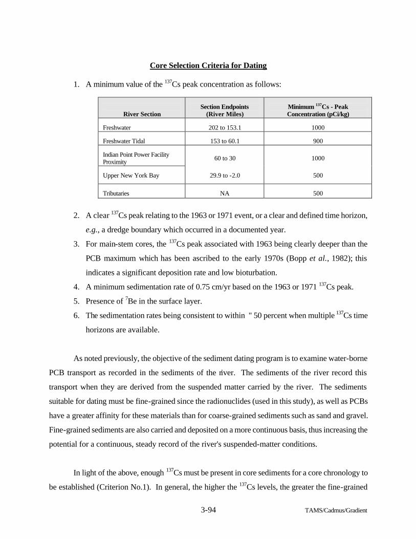
3-94 TAMS/Cadmus/Gradient
Core Selection Criteria for Dating
1. A minimum value of the 137Cs peak concentration as follows:
River Section
Section Endpoints
(River Miles)
Minimum 137Cs - Peak Concentration (pCi/kg)
Freshwater
202 to 153.1
1000
Freshwater Tidal
153 to 60.1
900
Indian Point Power Facility Proximity
60 to 30
1000
Upper New York Bay
29.9 to -2.0
500
Tributaries
NA
500
2. A clear 137Cs peak relating to the 1963 or 1971 event, or a clear and defined time horizon,
e.g., a dredge boundary which occurred in a documented year.
3. For main-stem cores, the 137Cs peak associated with 1963 being clearly deeper than the
PCB maximum which has been ascribed to the early 1970s (Bopp et al., 1982); this
indicates a significant deposition rate and low bioturbation.
4. A minimum sedimentation rate of 0.75 cm/yr based on the 1963 or 1971 137Cs peak.
5. Presence of 7Be in the surface layer.
6. The sedimentation rates being consistent to within " 50 percent when multiple 137Cs time
horizons are available.
As noted previously, the objective of the sediment dating program is to examine water-borne
PCB transport as recorded in the sediments of the river. The sediments of the river record this
transport when they are derived from the suspended matter carried by the river. The sediments
suitable for dating must be fine-grained since the radionuclides (used in this study), as well as PCBs
have a greater affinity for these materials than for coarse-grained sediments such as sand and gravel.
Fine-grained sediments are also carried and deposited on a more continuous basis, thus increasing the
potential for a continuous, steady record of the river's suspended-matter conditions.
In light of the above, enough 137Cs must be present in core sediments for a core chronology to
be established (Criterion No.1). In general, the higher the 137Cs levels, the greater the fine-grained
3-95 TAMS/Cadmus/Gradient
sediment content and the higher the sediment deposition rate. The minimum concentrations of the 137Cs
maxima listed by river section are intended to select cores with sufficient fine-grained sediment
content. Although core 137Cs levels decrease gradually in the downstream direction above the salt
front, below the front, the Indian Point nuclear power facility has released additional 137Cs into the
Hudson. Thus the minimum 137Cs criterion is increased below RM 60. In addition to the presence of 137Cs, a clear 137Cs peak, defining 1963 or 1971, is imperative for using 137Cs as an event-marker
(Criterion No. 2). If there is no clear maximum, there is no point upon which to determine the
sedimentation rate.
The PCB concentrations in the core slices were reviewed in conjunction with the radionuclide
profiles. Historical analyses of cores collected throughout the Hudson have allowed ascription of the
sediment PCB maximum to the early 1970s (Bopp et al., 1982). Based on these results from the
literature, a third criterion was defined for cores containing the 1963 137Cs maximum. Criterion No. 3
requires that the PCB and 137Cs maxima occur in separate layers, with the PCB maximum at the
shallower depth. Cores not meeting this criterion have probably had significant bioturbation or
irregular deposition histories. Having a consistent sedimentation rate throughout the history of a
coring site is requisite for reliable dating and interpretation.
Particulate matter tagged with radionuclides accumulate in quiescent zones of the Hudson
River at rates from 0.5 to greater than 5 cm/yr, depending upon location. In general, the rates do not
appear to fluctuate widely but remain within a one-centimeter range, i.e., " 1 cm/yr at a given location.
If the sedimentation rate is too low the resolution of the layers will be poor and year assignment to a
particular depth would be difficult. A minimum deposition rate of 0.75 cm/yr was defined as
Criterion No. 4. The 1954 137Cs appearance provides an event for confirming the sedimentation rate
obtained from the 137Cs maximum. Agreement between two or more dating horizons is defined in
Criterion No. 6.
The presence of 7Be in the surface layer, Criterion No. 5, confirms the presence of sediment
which has been deposited within a year from the time of collection. In a core lacking 7Be, the age of
the surficial sediments cannot be determined with accuracy. The location may have been disturbed by
scour processes or it may simply represent a currently non-depositional environment. For example,
Core 26 from RM 194.1, collected near the eastern shoreline, is lacking 7Be in the surficial layer.
3-96 TAMS/Cadmus/Gradient
Field observations during low-flow conditions during the summer of 1993 indicated that this core
location was exposed to air. Although the sediment core was collected the previous fall when the
location was submerged, it is likely that similar exposure had also occurred in previous summers
under similar low flow conditions. Recurrence of this type of event would probably significantly alter
the core chronology since no sediments would accumulate during this period and surface erosion
during rain events would be likely. As a result, this core was not used in the dating analysis.
For a core to be considered datable by the standard radionuclide method, Criteria Nos. 1, 2, 4
and 5 had to be met. If the 1963 137Cs maximum was used to date the core, then Criterion No. 3 had to
be met as well. In addition, if the 1954 horizon was present, then Criterion No. 6 had to be met as
well. Table 3-17 summarizes compliance with the criteria for dating the cores.
Factors Influencing Sediment Core Chronologies
Sediments in the Hudson are influenced by a number of factors including suspended-matter
deposition, sediment scour, biological activity, anthropogenic activities and in situ geochemical
processes. The ability to obtain a core with a datable chronology from a given location requires that
all but the first factor have had minimal effect on the sediments there. The criteria discussed
previously were designed so as to select cores from locations where these other factors were
unimportant. The potential impacts of these factors in establishing sediment core chronologies are
discussed below.
Variations in river flow can result in changes in the sediment deposition rate as well as mixing
of surficial sediments. In years of higher river flow, suspended-matter loads are likely to be higher
and deposition is likely to be greater. This variability limits the core resolution to two to four years.
The mixing of surficial sediments by higher flows is largely avoided at the high-resolution coring sites
since these are specifically selected for their quiescent conditions. A smooth 137Cs profile in the core
serves to confirm this selection since significant reworking or sediment removal would (likely) have
destroyed the integrity of the 137Cs record.
Benthic invertebrates living in the surface sediment can cause mixing as they move vertically
or horizontally through the sediment. This phenomenon is referred to as bioturbation. This activity
3-97 TAMS/Cadmus/Gradient
would serve to smooth sediment core profiles so as to largely remove the PCB and 137Cs maxima, thus
making the core undatable. The majority of benthic invertebrate activity is generally limited to about
five centimeters below the sediment-water interface.
Olsen et al. (1981) states that vertical mixing due to bioturbation in areas of high depositional
rate, i.e., greater than 3 cm/yr, has a minor impact on the core chronology. Greater sediment mixing
occurs in sediments underlying more saline water (5 to 30 parts per thousand [ppt]) and lower mixing
occurs in less saline areas of 0 to 5 ppt salinity. The more extensive mixing is generally attributed to
the higher levels of biological activity in the more saline regions. Most of the Phase 2 sediment cores
were collected in freshwater areas. Eight of the 11 dated main-stem Hudson River cores are from
locations above the salt front at about RM 60. Sediment mixing may also result from gas bubble
formation. As gas bubbles, resulting from biochemical processes in the sediment, naturally rise
through the sediments, some mixing may result. However, on the basis of Olsen's research, mixing due
to these phenomena is likely to have a minor impact on whether cores meet the dating criteria and thus
will not interfere with establishing core chronologies.
Anthropogenic disturbances such as dredging may disturb an area sufficiently that a core
collected from this location may not be datable. However, if enough sedimentation has occurred since
the dredging event, the dredge horizon itself becomes a dating event. For example, Core 6 (RM 43.2)
was collected from Lents Cove which was dredged in the late 1960s. The effects of the dredging can
be seen very clearly in the sediments underlying the 1971 137Cs maximum (see Figure 3-50).
In situ geochemical processes have the potential to change or destroy sediment core
chronologies. Porewater processes may permit the migration of 137Cs, 7Be and PCBs within the
sediments. However, Olsen et al. (1979, 1981) examined this concern for 137Cs and found no
evidence for this in Hudson River sediments. Presumably, this was prevented by the high sediment-to-
water partition coefficient for 137Cs. Similarly, both PCBs and 7Be have high partition coefficients and
it is expected that porewater migration would have little effect on core chronologies. (Given the
presence of fine-grained particles in these core locations which limit porewater movement, significant
porewater transport is not anticipated in these areas. These coring sites are not typical of the general
sediment type found in the Hudson River; they are more consistently fine-grained and therefore
represent only a small portion of the Hudson River sediments.) However, in situ processes have been
3-98 TAMS/Cadmus/Gradient
shown to alter the congener mixture within Hudson River sediments (Bopp et al., 1985; J. Brown et
al., 1987; J. Brown et al., 1984). This effect is discussed later in this report.
These factors (sediment deposition, sediment scour, biological activity, anthropogenic
activities, and in situ geochemical processes) can affect the certainty of the assigned dates of
deposition. In addition, the uncertainty of the assigned dates is not constant over the length of the core,
but rather is a function of the distance from "known" time points, e.g., the top layer is 1992. Thus, the
deposition rates presented in this report should be considered long-term averages.
For the cores selected for dating, the sedimentation rates determined by 137Cs and 7Be are
consistent with each other and do not vary more than " 50 percent at a given location. In addition,
despite the uncertainties associated with this dating methodology, the relationships of PCBs
concentration and patterns among contaminant bearing layers are consistent both within individual
cores and among the dated Hudson River cores downstream of the GE facilities. Also, profiles
generated from 1992 sediment cores are similar for comparable time periods to those of cores
collected in 1984 from approximately the same locations by LDEO. An example of this is shown in
Figure 3-52 for 1984 and 1992 cores collected at RM 188.5. The 1992 core (i.e., Core 19) shows a
lower deposition rate which caused the 137Cs peak to appear at a shallower depth. Also, the 1992
core probably contained less fine-grained material which would explain the lower 137Cs concentration.
Nevertheless, these two cores possess the same features, i.e., a distinct 137Cs appearance, a sharp and
clear peak, and a steady decline following the maximum in the more recent sediment.
Core Chronologies
Based on the core selection criteria described previously, 14 cores were dated in order to
calculate average deposition rates. Eight cores, consisting of Core 10 (RM 88.5), Core 12 (Mohawk
River), Core 17 (Batten Kill), and Core 18 (RM 185.8), Core 19 (RM 188.5), Core 21 (RM 177.8),
Core 23 (RM 189.3), and Core 27 (RM 202.9) were dated based on the 1963 137Cs maximum. Three
cores, Core 6 (RM 43.2), Core 7 (RM 43.2), and Core 2 (RM -1.9), were dated using the 1971 137Cs
peak. Three cores, Core 11 (RM 143.5), Core 22 (RM 177.8), and Core 24 (Hoosic River) were
dated on unique information as discussed below. While the three tributary cores, i.e., Core 12
(Mohawk River), Core 17 (Batten Kill), and Core 24 (Hoosic River) and the background station, Core
3-99 TAMS/Cadmus/Gradient
27 (RM 202.9) do not meet all of the selection criteria, core chronologies were estimated in order to
provide some information on sediment deposited within the last ten years. Note that the core numbers
were assigned by the order in which they were collected and are not in river mile sequence.
Core 11 at RM 143.5 in the Albany Turning Basin was found to contain no 137Cs maximum as
shown in Figure 3-51. However, a minimum sedimentation rate for the core was calculated based on
the absence of a predominant peak for PCBs down to 104 centimeters in depth and knowledge of the
history of dredging in the area. Since this area had been dredged extensively circa 1971, the 1963 137Cs maximum would not be present in a core collected from this location. A core collected from this
location in 1977 by LDEO showed a very high sedimentation rate, using the PCB maximum for dating.
Based on the LDEO results, the twenty years of deposition since the dredging event should have
accumulated at least 100 centimeters of sediment. The deepest layer of the Phase 2 core was found to
contain more than 17 mg/kg of PCBs, the highest value found in the Lower Hudson cores. This value
represents a sharp increase relative to the concentration in the 100 cm of sediment above it and was
assumed to represent the latter portion of the early 1970s PCB maximum. Based on the history of
dredging in the area, the results obtained by LDEO in 1977 at this site, and the sharp rise in PCB level
in the deepest layer, the bottom layer of this core was assigned to 1973, yielding a minimum
deposition rate of 5 cm/yr.
The surface layer of this core, with a depth of two centimeters, was found to contain 7Be.
Because the second and third layers, i.e., at 2 to 4 cm, and 4 to 6 cm, respectively, were analyzed
several months later, the opportunity to confirm the high sedimentation rate based on the 7Be data was
lost. Nonetheless, it is estimated that the 5 cm/yr deposition rate obtained for this core is sufficiently
accurate for the purposes of this program.
Core 22, collected at RM 177.8, does not meet the criteria described previously but was dated
by matching the 137Cs and PCB patterns with depth against those of Core 21, its duplicate.
Specifically, Core 22 appears to have a 50 percent higher deposition rate than Core 21. This
difference in sedimentation rate may be attributed to the fact that Core 22 was collected more than 100
feet closer to the shoreline than Core 21 since sedimentation rates are specific to particular locations
and their conditions. Although both cores are of comparable length, Core 22 does not penetrate to the
1963 137Cs maximum.
3-100 TAMS/Cadmus/Gradient
The chronologies for the duplicate pair of Cores 6 and 7 at RM 43.2 are based on the 1971
137Cs event also using 60Co to confirm the 137Cs maximum as derived from the 1971 Indian Point
release. Since this location was dredged in the early 1970s (Bopp, 1993 pers. comm.), the presence
of a second, deeper 137Cs maximum was not expected. Although Core 6 did not contain 7Be, its
duplicate, Core 7, as well as cores previously collected at this location, did contain 7Be. Therefore,
these cores, as a pair, satisfy the necessary criteria.
Core 2, collected at RM -1.9, was dated on the basis of the 1971 137Cs event. This was
confirmed by the parallel 60Co profile in this core also observed in Core 6 collected from a location
adjacent to the Indian Point nuclear power facility.
As can be seen, the number of cores which meet all the criteria are limited. This stems from a
number of conditions. In general, the program was more successful in re-occupying historical coring
sites than in establishing new ones. This is a direct result of the difficulty in finding suitable sites. In
some cases, particularly in the Harbor area, it appeared that a suitable site had been found but the core
recovery was too short relative to the high deposition rate at that location. Other cores lacked 7Be-
bearing sediments or exhibited significant bioturbation. However, in several cases it was still
possible to overcome some of these shortcomings and establish the core chronology on the basis of
unique information.
As previously noted, the three tributary cores, i.e., Core 12 (Mohawk River), Core 17 (Batten
Kill), and Core 24 (Hoosic River), as well as the background station, Core 27 at RM 202.9, do not
meet all the criteria but still provide some information on sediment deposited within the last ten years.
Criterion No. 3, regarding the separation of the 137Cs and PCB maxima, is not applicable to the
tributaries since there are no documented major releases of PCBs associated with the tributaries. The
Mohawk River core meets the remaining criteria. The Batten Kill core meets all the remaining
criteria, with the exception of containing 7Be in its surface layer. However, the archived (A) core
collected from the site at the same time contained 7Be in the top slice. This slice was analyzed for
PCBs and was shown to match the top slice in Core 17. Thus Core 17 was able to satisfy all
applicable criteria and was dated. Core 24 from the Hoosic River only satisfied the 7Be criterion
although all core layers contain 137Cs indicating post-1954 deposition. On this basis, 7Be was used to
3-101 TAMS/Cadmus/Gradient
establish an upper bound on the deposition rate so that the core chronology could be estimated. The
core collected at RM 202.9 provides information regarding historical background levels of PCBs in
suspended matter. The sedimentation rate of this core was determined based on the 137Cs peak at a
depth of 34 centimeters. The low levels of 137Cs suggest some bioturbation at this site. However, it is
still useful for establishing background conditions.
Figures 3-53 through 3-55 show the 137Cs and PCB profiles for the dated cores. Note that the
x-axis scales for 137Cs and PCB concentrations are adjusted for each core to match the core depth.
These plots show the profiles and relative positions of the 137Cs and PCB maxima. Table 3-18 lists
the calculated sedimentation rates for the dated sediment cores as well as the primary radionuclide
event used to date each core.
Approximate core chronologies were established for the cores which satisfied the core
collection criteria. The coring and slicing methodology used as part of the Phase 2 sampling program
provided greater resolution near the surface and less resolution at depth. In general, the first eight
centimeters were sliced in 2-cm intervals; the remainder of the core was sliced in 4-cm intervals.
Thus more resolution was obtained for the most recent sediments, which are of greatest interest to the
program since these sediments indicate the latest trends of water column transport of PCBs. A
sedimentation rate was assigned to each core meeting the core selection criteria by assigning a year to
at least one well-defined event or horizon identified in the core. The sedimentation rate was
calculated by taking the depth of center of the layer (slice) containing the event and dividing by the
time interval, where the time interval is the year assigned to the event (either 1963 or 1971 when
based on 137Cs) subtracted from the time of collection, i.e., 1992, yielding a rate in centimeters per
year.
For core chronologies based on a 7Be presence, the age of the 7Be-bearing layer was assumed
to be one year. For example, the center of a 2-cm slice was assigned as 1991 since all cores were
collected in 1992. This would yield a deposition rate of 1 cm/yr.
While a single 137Cs event permits the estimation of the average deposition rate, it is unlikely
that the sedimentation rate was constant over the entire depositional period. Seasonal variations in
deposition rate as well as annual variations are likely, although, given the intended temporal
3-102 TAMS/Cadmus/Gradient
resolution of two to four years, these effects should be minor. However, some degree of uncertainty is
associated with all assigned dates of deposition.
In summary, 14 high-resolution sediment cores including those from three tributaries and a
background core were successfully dated. These chronologies confirm historical work performed by
LDEO on dated Hudson River sediment cores. 7Be was observed in sediment of 12 of the 14
locations, thus confirming the presence of post-1991 deposition. The water column PCB transport
suggested by these core chronologies is discussed in the following two sections.
3.3.2 Surface Sediment Characterization
A basic tenet in the use of dated sediment cores as indicators of long-term, i.e., historical, PCB
input, transport, and degradation in the Hudson River is that the PCB content of the sediment is
representative of the water column PCB loading. A comparison of the PCB content of recently
deposited surficial sediment, within both the Upper and Lower River, with that of the spatially
corresponding suspended matter verifies this assumption. That is, the PCB content of the surficial
sediment is consistent, both in congener distribution and concentration, with the PCB content of the
suspended-matter samples, collected as part of the Phase 2 water column transect sampling program.
Only core tops bearing beryllium, which is indicative of recent deposition as discussed in Subsection
3.3.1, are included in this analysis. In addition, only core tops with total PCB concentrations less than
30,000 µg/kg (30 ppm) are compared to the suspended-matter samples on a congener basis. The
rationale for this latter criterion is that, as discussed later (Section 4.3), cores with total PCB
concentrations greater than 30 ppm tend to exhibit evidence of dechlorination. As a result, the
congener patterns associated with these cores are altered and, as such, are no longer representative of
the congener patterns of the originally deposited suspended matter.
As is evident in the comparison of surficial sediment in the Upper and Lower River cores with
the corresponding suspended-matter samples collected during the Transect 4 high-flow event (see
Figure 3-56), both exhibit very consistent congener distributions. In addition, as illustrated in Figure
3-57, the congener distributions associated with the TI Pool suspended-matter samples, collected
during the Phase 2 winter and summer, low-flow sampling efforts, compare well with that of the TI
Pool Core 23 core top. Similarly, the congener distributions associated with the suspended-matter
3-103 TAMS/Cadmus/Gradient
samples collected at the Albany Turning Basin during the Phase 2 winter and summer, low-flow
sampling efforts, compare well with that of the Albany Turning Basin core top (see Figure 3-58).
In addition to the similarity between congener patterns, the suspended-matter samples and the
corresponding core tops also exhibit comparable total PCB concentrations (see Table 3-19). This
congruence, both in congener pattern and total PCB concentration, indicates that the PCB content in the
overlying water column, as characterized by the PCB content of the suspended-matter samples, is
represented by the corresponding core tops.
However, it is important to note that while the congener patterns of the suspended-matter
samples, collected during the winter and summer low-flow events, are consistent with those of the
corresponding core tops, the core tops are best represented by the Transect 4, high-flow suspended-
matter samples. This is an expected result since it is assumed that the sediment acts as an integrator of
the suspended-matter loading. The spring-flood event, which is generally less than a month in
duration, introduces approximately one-third of the yearly PCB load to the water column. The
remaining two-thirds of the yearly PCB load is introduced throughout the remaining 11 months of the
year. Therefore, the core tops should be best represented by the high-flow suspended-matter samples
since these samples represent the largest pulse input of PCBs to the water column. However, the core
tops should, and do, exhibit consistency with the PCB loading introduced to the water column during
the remaining months of the year.
The comparability of the surficial sediment PCB inventory with that of the corresponding
suspended-matter samples has important implications since it provides independent verification of the
use of the high-resolution sediment coring data as a record of the long-term, i.e., historical, PCB input
and transport in the Hudson River. Specifically, because the suspended matter is in effective
equilibrium with the water column dissolved phase (see Section 3.1), variation in the historical, water
column PCB inventory should be directly represented by a commensurate variation in the sediment
PCB inventory. Further, by using appropriate partition coefficients, the sediment record can provide
information on the historical distribution of PCBs between the dissolved and suspended-matter phases.
3-104 TAMS/Cadmus/Gradient
In summary, an important conclusion that can be drawn from the comparison of the surficial-
sediment and suspended-matter PCB inventories is that the PCB loading, exhibited by the dated
sediment records, is representative of the contemporaneous water column PCB loading. However, the
sediment cores best represent the PCB loading associated with the high-flow, spring-flood events.
Thus, while daily water column monitoring provides the most accurate record of the characteristics of
the PCB loading to the water column, the analysis of dated sediment cores is an effective tool in
estimating the long-term, water column PCB loading.
3.3.3 Water Column Transport of PCBs Shown by Sediment Deposited After 1975
As discussed previously, the primary objective in performing the high-resolution coring
program was to obtain an independent record of water column PCB transport throughout the Hudson
River for the 1982 to 1992 time period. In order to place this period in perspective with previous
Hudson River PCB transport events, core chronologies were examined back to 1975. The selection of
datable cores from the Hudson (including two duplicate pairs) chosen for this analysis is based on
their well-defined chronologies. The cores used in this analysis are listed in Table 3-20.
The analysis of the historical water column transport of PCBs based on these cores was
performed on two levels, i.e., for total PCBs, and on a congener-specific basis. Examining total PCBs
provides information on the general trend of PCB transport in the last 10 to 15 years. The congener-
specific analysis explores the size and type of additional inputs to the Hudson River below the TI Dam
(RM 188.5).
Examination of Water Column Transport of Total PCBs Since 1975
The total PCB analysis of the high-resolution sediment cores yields two major findings. First,
there was a substantial decline in PCB levels between 1975 and 1982 followed by a plateau to 1990
in all regions of the Hudson River studied. An example of this trend with time is shown in Figure 3-59
for Core 19, collected at RM 188.5. Second, PCB concentrations decrease steadily downstream from
the TI Dam at RM 188.5 in sediments deposited during the same time period. This trend is shown in
Figure 3-60 for sediment deposited after 1990, generally represented by the top slice of each core.
Parallel trends in water column transport can be inferred from these results.
3-105 TAMS/Cadmus/Gradient
The implication of the first finding is that PCB loads originating above the TI Dam have
leveled off within the last 8 to10 years. However, this analysis cannot differentiate between the load
from the TI Pool and the loads originating above Rogers Island, such as GE Hudson Falls facility
releases. In subsequent discussions, the loadings from the GE Hudson Falls facility source, other
loadings between Bakers Falls, Rogers Island, and the TI Pool loading will be referred to collectively
as the combined TI Dam load, since the load at the TI Dam represents the sum of these loadings. The
second finding indicates that the area above the TI Dam is the primary PCB source to most of the
Hudson. Based on the low PCB levels in the tributary cores, the tributaries to the Upper Hudson do
not contribute substantial PCB loads. The Mohawk River core and its inferred loading are consistent
with the Phase 2 water column monitoring results which indicate that the Mohawk contributes on
average approximately 10 percent of the total PCB load.
Evidence of decrease and subsequent leveling off of PCB loading to the water column,
illustrated by Figure 3-59, is found in the results from all dated Hudson River sediment cores. Figure
3-61 shows the total PCB trend with time in eight of the dated Hudson River cores, including two
duplicate pairs, representing the entire region below Fort Edward. In each core, the decline in PCB
levels between 1975 and 1982 represents the largest single change. For the interval 1982 to 1992 the
PCB concentration appears to level off with time, suggesting that substantial long term decline is
unlikely. Little evidence of the relatively large 1991 to 1992 releases attributed by GE to the Hudson
Falls facility is discernible. This suggests that these releases are small in scale relative to conditions
ten years prior or that the time of core collection (Fall 1992) may have been too close to the releases
for the impact to be observed. The majority of the large releases measured at RM 194.6 at Rogers
Island occurred in September 1991 and June through October 1992. Some evidence for an increase in
the loadings is suggested when normalizing for 137Cs as discussed below.
Evidence of a decrease in PCB loading to the water column downstream of the TI Dam, can be
seen in each of several time intervals representing the last 17 years of deposition. Figure 3-62 shows
the relationship between total PCBs and river mile for the periods 1975 to 1981, 1982 to 1986, 1987
to 1990, and 1991 to 1992. In each case there is a decline in PCB concentration with distance
downstream from the TI Dam at RM 188.5. From Stillwater at RM 177.8, the decrease downstream is
generally consistent, with no apparent intermittent increases. Note that the trends shown in Figure 3-
3-106 TAMS/Cadmus/Gradient
62 begin with the core collected at RM 188.5 (Core 19), rather than with 189.3 (Core 23) as is seen in
Figure 3-60. The first two connected data points in Figure 3-60, representing Cores 23 (RM 189.3)
and 19 (RM 188.5) respectively, were collected from the TI Pool. However, there is a large
concentration difference between them.
While this difference may be due to their proximity to source areas such that suspended-matter
PCB concentrations are not well homogenized at the time of deposition, incomplete mixing should
serve to either raise or lower the PCB concentrations in the sediments settling at a given location.
This process should introduce random variability in PCB concentration within the sediments whereas
the concentrations in sections of Core 23 are consistently lower than those of Core 19 for sediment
deposited after 1975. It is more likely that the lower PCB concentrations observed in Core 23 are due
to its collection from the Moses Kill delta in the TI Pool. This location would tend to collect a
mixture of Hudson River suspended matter with a disproportionately large amount of Moses Kill
suspended matter. This scenario would tend to preserve the overall PCB relationship with time as
well as the congener composition (see Subsection 3.3.2) while lowering the magnitude of the total
PCB concentration. On this basis, the PCB concentrations recorded in Core 19 at RM 188.5 are
considered more reflective of historical suspended-matter concentrations in the TI Pool, and are used
to represent the Pool in subsequent figures.
Much of the variability in the downstream trends can be removed by normalizing the data to 137Cs to account for differences in the amount of fine-grained material among the cores since both
PCBs and 137Cs preferentially bind to smaller sized particles (see Subsection 3.3.1). Thus,
normalizing to 137Cs removes variations in the PCB concentration which are related to the percent of
fine-grained matter in a sample. This normalization scheme assumes that the average 137Cs
concentration on tributary suspended matter is approximately the same as that originating from the
Upper Hudson. This assumption is supported by the 137Cs content of surface sediments from RM 177.8
near Stillwater to Upper New York Bay as shown in Figure 3-63. This figure shows the 137Cs content
of the 0 to 2 cm interval of all sediment cores collected. From RM 177.8 downstream, there is no
systematic trend in the 137Cs levels, indicating that additional tributary contributions of 137Cs are
similar on average to those found at RM 177.8. Above RM 177.8, there is much greater variability,
the source of which is unclear.
3-107 TAMS/Cadmus/Gradient
The PCB to 137Cs ratios as a function of river mile for the 1975 to 1981, 1982 to 1986, 1987 to
1990, and 1991 to 1992 time periods are shown in Figure 3-64. In each period, the decrease in the
PCB/137Cs ratio downstream is clearly evident. The overall PCB to 137Cs ratio trend with time can be
examined by superimposing the four trends as shown in Figure 3-65. In general, a reduction in
sediment PCB concentrations (and, by inference, PCB loadings) is evident with the rate of change
becoming smaller over time. The 1991 to 1992 results at RM 177.8 (Stillwater) and RM 143.5
(Albany) indicate a rise in the combined TI Dam loading consistent with the GE water column
monitoring results discussed in Subsection 3.3.4. However, this slight change in trend may be within
the range of uncertainty of the measurement technique.
The consistent decline of PCB concentrations downstream of the TI Dam suggests that dilution
of the load measured at the dam by subsequent tributary input is a major factor influencing downstream
PCB concentration. To further explore this issue, TAMS/Gradient prepared an estimate of the
expected suspended-matter concentrations as recorded in the sediment cores based on an assumption
of conservative PCB transport, i.e., that dilution during water column transport is the only factor
affecting suspended matter PCB concentrations. This estimate ignored any changes in concentration
due to geochemical or biochemical processes within the water column and assumed no additional PCB
inputs besides those originating above the TI Dam. Calculated changes in the PCB to 137Cs ratio were
scaled based on the increases in the watershed drainage basin area down to RM 43.2 at Lents Cove. It
is assumed that an increase in drainage basin area is directly proportional to an increase in flow.
Further, it is assumed that 137Cs is deposited equally everywhere such that suspended-solids loading
from tributaries should contain comparable concentrations of 137Cs as that from the Upper River but
without a corresponding PCB load. Therefore, tributary input of suspended solids, proportional to the
flow contribution of the tributary, should serve to dilute the suspended matter PCB concentration
without an associated dilution of the suspended matter 137Cs concentration, thereby decreasing the PCB
to 137Cs ratio in direct proportion to the flow increase. For example, a doubling of the drainage basin
area and, as a result, doubling of flow between coring locations would halve the PCB to 137Cs ratio.
Estimation of suspended-matter PCB concentration, originating from the combined TI Dam
load, upon its arrival in the Harbor is more complicated due to a number of factors. The salinity at
Lents Cove is about 1 ppt while that in the Harbor at RM -1.9 is approximately 15 ppt. Below the
Verrazano Narrows, the salinity increases to approximately 30 ppt (Garvey, 1990). Therefore, based
3-108 TAMS/Cadmus/Gradient
on salinity alone, the water in the Harbor would be expected to represent a 50:50 mixture of Lents
Cove water and seawater. Sewage effluent and local tributaries entering the Harbor would introduce
an additional 20 percent dilution by volume (Garvey, 1990), assuming it was PCB-free. The sewage
effluent contains an organic-rich, high suspended-matter load which should dilute the suspended-
matter PCB concentration even further. However, dilution is not the only factor affecting the
suspended-matter PCB to 137Cs ratio in the Harbor as is discussed below.
The partition coefficient for 137Cs in seawater is lower than that for freshwater, thus some loss
of 137Cs from suspended matter may occur in the saline region of the river. This would be reflected as
an increase in the PCB to 137Cs ratio. It should be noted that Harbor 137Cs levels are comparable to
those in the freshwater region of the Hudson as shown on Figure 3-63. In addition, salinity affects
PCB suspended matter-water partitioning as well. In particular, the mixing of saline water with
Hudson River fresh water causes the precipitation of dissolved organic carbon, presumably reducing
the PCB loads carried by this fraction and affecting the PCB distribution in the water column (see
Section 3.1). In addition, the presence of salt raises the PCB suspended matter-water partition
coefficient, which would serve to increase the PCB to 137Cs ratio. Thus, while dilution by seawater
and sewage would be expected to decrease the PCB to 137Cs ratio, the change in geochemical
parameters (e.g., partition coefficients) would serve to increase this ratio. PCB additions by sewage
would be expected to increase this ratio as well. A reliable estimate of these effects is not possible
given the current level of understanding of PCB geochemistry and, therefore, no predicted value was
calculated for RM -1.9. It is noted that the PCB to 137Cs ratios at RM -1.9 generally agree within " 25
percent of those at RM 43.2 in spite of all these considerations.
Using the PCB to 137Cs ratio measured in Core 19 at RM 188.5 near the TI Dam as the initial
input, TAMS/Gradient calculated the expected downstream concentrations for each time interval. The
calculated PCB to 137Cs ratios are shown in Figure 3-66 together with the measured values for
sediment deposited after 1990. The PCB to 137Cs ratios of the tributaries are indicated on the diagram.
The difference between the calculated and measured ratios for RM 177.8 near Stillwater appears too
large to be explained by dilution of the combined TI Dam load alone. The difference between the
calculated and measured values near Stillwater (RM 177.8) is even greater for earlier periods as
shown in Figure 3-67. The apparent PCB loss from the water column, as suggested by the decreased
PCB to 137Cs ratios near Stillwater, may be related to a number of factors such as incomplete mixing of
3-109 TAMS/Cadmus/Gradient
PCBs in the water column due to proximity to the sources, bedload movement stopped by the TI Dam,
and PCB deposition by particle settling between the coring locations. As shown in Figure 3-63, 137Cs
levels are highly variable above RM 177.8 which may be related to this issue. Based on this finding,
the conservative transport calculation was revised to begin at RM 177.8 near Stillwater and is also
shown in Figures 3-66 and 3-67.
The calculated conservative transport results, beginning with the Stillwater measurements for
the four time intervals from 1975 through 1992, are shown in Figure 3-68. As shown in Figure 3-68,
from Stillwater downstream, the conservative transport model approximates the suspended-matter
PCB concentrations recorded in the cores quite well, to within "25 percent of the measured value for
the freshwater region of the river. Based on the success of this simple conservative transport
calculation, it appears that the combined TI Dam load represents the single, largest source of PCBs to
the entire freshwater Hudson constituting about 75 percent of the load as far south as River 88.5, 100
miles downstream.
The smooth and consistent trend of PCB concentrations with time within each core and with
river mile among cores downstream of the TI Dam suggests that the river PCB conditions are governed
by a limited number of sources and processes and that the processes are approaching a steady-state
balance. The general declining trend with time followed by a concentration plateau implies that there
has been a significant decline in PCB inputs to the river since the early 1970s, and specifically that the
events of 1991 to 1992 are small in scale relative to those of the early 1970s. In the interim, smaller
but steady PCB loads generated above the TI Dam have maintained PCB levels in the Hudson.
Assuming that the river conditions are approaching a steady state, historical data can be readily
extrapolated to future conditions.
In summary, the results presented above suggest the following interpretation of PCB transport
in the Hudson. Scouring of the TI Pool sediments from 1975 through the early 1980s dominated PCB
water column transport. This observation is also supported by the USGS data presented in Subsection
3.3.5. Subsequently, the water column transport became less dynamically driven (less scour) and less
variable temporally, presumably driven by sediment-water exchange with the TI Pool sediments and
releases originating above Rogers Island such as those from the GE Hudson Falls facility. This is
supported by both the Phase 2 water column mass transport data and the USGS data. (see Section 3.2

3-110 TAMS/Cadmus/Gradient
and Subsection 3.3.5, respectively). The conservative transport calculations suggest that from RM
177.8 at Stillwater to at least RM 43.2 at Lents Cove, the combined TI Dam load is the main
controlling factor in water column PCB transport and downstream water column concentrations.
Additional sources appear to be minor and PCBs generated above the TI Dam are transported
downstream relatively conservatively. This suggests that ultimately much of this PCB load is
transported directly out to the New York Bight.
3-111 TAMS/Cadmus/Gradient
Examination of Post-1975 Water Column Transport on a Congener-Specific Basis
Using the dated sediment cores discussed in the previous sections, it is also possible to
examine the historical water column PCB transport on a congener-specific basis. The dated sediments
record not only a measure of the water column total PCB level, but also the mixture of congeners
which comprised the water column inventory at the time of deposition. The examination of the
congener mixtures in a sediment core can provide useful information on the type and scale of Aroclor
releases over time.
This section examines historical water column transport throughout the Upper and Lower
Hudson with an emphasis on identifying the combined TI Dam load. In particular, this section shows
that it is possible to identify this load throughout the entire Hudson over the period from 1975 to the
present. On the basis of this identification, the fraction of the PCB load derived from the Upper
Hudson above the TI Dam is estimated at each location studied. These estimates indicate that the
combined TI Dam loadings comprise at least 75 percent to 85 percent of the load at RM 143.5 near
Albany and possibly half of the load at RM -1.9 in the Upper New York Bay during the period 1982 to
1992.
In the examination performed for the Phase 2 investigation, the congener mixture characteristic
of the combined TI Dam load is the obvious main focus. To this end, historical PCB loads were
examined as recorded in Upper Hudson sediment cores in order to uniquely identify or "fingerprint"
this combined source. As discussed in Section 4.3, much of the PCB-bearing sediment in the Upper
Hudson exhibits substantial dechlorination. In these sediments, the "fingerprint" is largely lost.
However, it is still possible to examine total PCB transport from these sediments on a total PCB basis,
as discussed previously in this section. This discussion will involve a subset of cores where
dechlorination is not prevalent.
The farthest-upstream sediment core where dechlorination is not a significant factor is located
at RM 177.8 near Stillwater. As discussed in Section 3.2 and Subsections 3.3.2 and 3.3.5, historical
and current water column records show that the PCB loading at Stillwater is essentially the same as
that at the TI Dam, making this sediment core a valuable record of the combined TI Dam load history.
This core actually lies just upstream of Stillwater, outside the town limits and will be referred to as
3-112 TAMS/Cadmus/Gradient
�near Stillwater� in subsequent discussions. However, because there are no substantial tributary
inputs between this location and the water column sampling station at RM 168.3, both the water
column PCB load and PCB concentrations are expected to be constant between these locations.
Therefore, results at this coring location and the Stillwater water column station at RM 168.3 should
be comparable.
In order to examine the historical transport of PCBs downstream from Stillwater, data from
four additional sediment cores were included in the analysis. These cores represent conditions at RM
143.5 near Albany (Core 11), RM 88.5 near Kingston (Core 10), RM 43.2 in Lents Cove (Core 6) and
RM -1.9 in Upper New York Bay (Core 2). These cores were selected based on satisfaction of the
dating criteria described previously. The original core sites were selected, in part, based on roughly
equal spacing downstream from Stillwater. Note that the Lents Cove and Upper New York Bay sites
are located below the salt front. As noted above, this examination is limited to sediments deposited
since 1975.
The loading of PCBs generated upstream of RM 177.8 is clearly documented by the sediment
record at Stillwater. Note that two cores (Nos. 21 and 22) were collected from this site. Good
agreement was found between the two cores for comparable time horizons based on matched 137Cs
profiles as shown in Figure 3-69. This figure represents the PCB congener pattern normalized to
BZ#52 for 1991 to 1992 deposition at RM 177.8. Note that the congener patterns are nearly identical
in spite of the fact that the total PCB concentration of the two core slices were 5.0 and 12.5 mg/kg, a
relative difference of 86 percent. Based on this comparison, it appears that the congener pattern is
preserved in the sediment independently of the total PCB concentration. Thus, if conservative
transport is the main process governing water column PCB levels, then the congener pattern recorded
at RM 177.8 should be preserved in the downstream cores in sediments of similar age. Note that the
relative difference between Cores 21 and 22 was reduced to 62 percent when the total PCB
concentration was normalized by 137Cs. The use of PCB to 137Cs ratio is discussed previously in this
section.
The information presented in Figure 3-69 and in most of the remaining figures in this section is
presented on a normalized basis. This normalization was performed in order to simplify comparisons
of congener patterns among various types of media independently of the absolute congener
3-113 TAMS/Cadmus/Gradient
concentrations. The normalization method involves the division of all congener concentrations by the
concentration of congener BZ#52. In this manner, the concentration of BZ#52 is set at 1.0 for all
mixtures. Congeners in mixtures at concentrations greater than that of BZ#52 have normalized values
greater than 1 and congeners at concentrations less than that of BZ#52 have normalized values less
than 1. BZ#52 was selected as the normalizing parameter based on its presence in Aroclor 1242, the
main Aroclor used by GE and on its reported resistance to degradation or dechlorination in the
environment. (Bopp et al., 1985; J. Brown et al., 1984).
Only one of the two cores collected at RM 177.8 near Stillwater extended down to sediments
deposited prior to 1954. This core, Core 21, will be used here to represent the congener pattern of the
combined TI Pool load over the period 1975 to 1992 since its dating horizons have less uncertainty.
Since the subsequent discussions deal only with the congener pattern and not the absolute PCB
concentrations, this choice has little effect on the conclusions as supported by the close congener
pattern agreement shown in Figure 3-69.
As was discussed in Chapter 2 and in the Phase 1 Report (TAMS/Gradient, 1991), reported
GE PCB usage has consisted of varying mixtures of several Aroclors, principally including Aroclors
1016, 1242 and 1254. It is evident in the sediment record near Stillwater that at least the latter two
Aroclors plus Aroclor 1260 have been present in the water column mixture right up to the most recent
deposition. Figure 3-70 shows the congener composition of the most recent sediments deposited at
Stillwater in comparison with the congener composition of Aroclors 1242, 1254 and 1260.
It is evident in Figure 3-70 that the majority of the congeners detected in the Stillwater post-
1990 sediments occur in Aroclor 1242. However, several more-chlorinated congeners are also
present in substantially greater proportion in recent Stillwater sediments than that found in unaltered
Aroclor 1242. The most likely Aroclor responsible for these congeners, based on the reported GE
uses, is Aroclor 1254. This mixture is compared to the pattern at Stillwater in the second diagram of
Figure 3-70 and correlates well with many of the higher congeners. However, this mixture does not
contain all of the more-chlorinated congeners found near Stillwater. Specifically, at least eight
detected target congeners do not occur in Aroclor 1242 or Aroclor 1254. A possible Aroclor mixture
for these congeners is Aroclor 1260. This Aroclor is compared with Stillwater 1991 to 1992
sediments in the third diagram of Figure 3-70. Note that this diagram has two vertical scales in order
3-114 TAMS/Cadmus/Gradient
to simplify the comparison of the mixtures. Aroclor 1260 contains little BZ#52 and so most of its
normalized ratios are much higher than those in the sample. Aroclor 1260 contains the eight target
congeners required to match the RM 177.8 sample (Core 21).
The fourth diagram in Figure 3-70 represents a rough attempt to synthesize the Stillwater
mixture from the three Aroclors. The mixture can be represented as containing approximately 82
percent Aroclor 1242, 16 percent Aroclor 1254 and 2 percent Aroclor 1260, suggesting that the recent
TI Dam loads contain all three Aroclors. The level of uncertainty in the latter two percentages is
estimated to be " 50 percent of the value. The specific evidence for the presence of Aroclor 1260 in
the congener patterns recorded near Stillwater is given in Figure 3-71. The top diagram in this figure
is an expanded scale plot comparing Stillwater with Aroclors 1254 and 1260. Indicated on the plot
are eight target congeners found exclusively in Aroclor 1260 and present in the Stillwater sediments
for 1991 to 1992. In order for these congeners to be present in the sediments, the mixture must have
contained about 2 percent Aroclor 1260 as stated above. Because these are more-chlorinated
congeners, they cannot be synthesized in the sediments and must have been derived from an upstream
source. These congeners are not present in the background core collected at RM 202.9, and thus must
originate in the area between Bakers Falls and the TI Dam.
Additional evidence can be seen in the suspended-matter samples collected in the Phase 2
water column monitoring program. In Figure 3-56, the congener composition of the suspended matter
at several locations in the Hudson is presented on a mass-fraction basis. Note the presence of BZ#180
in all suspended-matter samples, in particular in suspended matter at RM 188.5 near the TI Dam and
RM 168.3 at Stillwater. As shown in Figure 3-70, this congener is a major component of Aroclor
1260 and is not contained in either Aroclor 1242 or Aroclor 1254. Thus, its detection is indicative of
the presence of Aroclor 1260 in the suspended matter at RM 188.5 and 168.3. To further explore this,
the suspended matter at RM 194.6 at Rogers Island for Transect 4, April 12 to 14, 1993, was
examined on a congener basis. This sample was chosen since Transect 4 contains a large PCB load
which originates above this sampling point. The congener composition of this sample may be
characteristic of the GE Hudson Falls facility releases.
The lower diagram in Figure 3-71 compares the more-chlorinated congener composition of
this sample with that of Aroclors 1254 and 1260. Again the eight target congeners unique to Aroclor
3-115 TAMS/Cadmus/Gradient
1260 are found in the suspended matter, proof of its presence in this sample. Figure 3-72 represents a
rough synthesis of the suspended-matter mixture at RM 194.6 based on Aroclors 1242, 1254 and 1260.
The Aroclor fractions were 94 percent, 5 percent and 1 percent, respectively. Both the surface
sediments and suspended matter confirm the presence of the three Aroclors in the water column. The
differences between the Aroclor proportions of the two samples are considered to be minor in light of
the different time periods represented by the samples and the distance between sampling points. The
surface sediment represents an average of 1991 to 1992 conditions downstream of the TI Dam while
the suspended matter represents a half-hour "snapshot" of water column conditions below Bakers Falls
but above the TI Pool. The differences between the two samples may represent variations in the
congener composition of the load at RM 194.5 over time since the more-chlorinated congeners in the
combined TI Dam load appear to originate upstream of Rogers Island.
The mixture of congeners recorded in the Stillwater sediments has a number of unique features
which enable it to be identified in sediments downstream. In addition to the unique downstream
mixture of the three Aroclors, a number of target congeners are present or absent relative to these
standard Aroclor mixtures which serve to make the overall mixture even more easily identified. In
particular, the ratios of congeners BZ#18, BZ#26 and BZ#47, relative to BZ#52 may serve
specifically to identify the TI Dam mixture. Other congeners also show significant differences relative
to the standard Aroclors but were not used here because they are non-target congeners, are subject to
uncertainties in quantitation due to chromatographic coelution, or are believed to be strongly affected
by dechlorination processes, either as reactants or products.
Using the Stillwater core, it is possible to examine the historical mixtures released into the
river. Figure 3-73 shows the congener patterns recorded at RM 177.8 near Stillwater from 1975 to
the present. These patterns were compiled as mean normalized ratios from the dated sediment
intervals corresponding to the given period. This figure shows that little variation has occurred in the
congener composition over the period 1982 to the time of sediment core collection in 1992. This is an
important conclusion because it simplifies identification of the combined TI Dam load at downstream
locations. The oldest sediments shown in Figure 3-73 show a small shift toward less-chlorinated
congeners. This suggests that the mixture originating upstream of Stillwater contained less Aroclor
1254 relative to post-1982 releases. Note that in spite of the apparent decrease in Aroclor 1254
3-116 TAMS/Cadmus/Gradient
components, Aroclor 1260 is still present in the 1975 to 1982 PCB mixture, based on the presence of
the target congeners shown in Figure 3-71. BZ#180 is clearly evident in all diagrams on Figure 3-73.
It is interesting to note the decrease in congeners BZ#56, 60, 70 and 74 with time. These
congeners appear to be very susceptible to loss, either within the sediment or during water column
transport. These four congeners appear to decrease significantly with depth without alteration of the
rest of the congener mixture, suggesting a selective destruction process. For the four diagrams shown
in Figure 3-73, the apparent loss of these four congeners increases as both the age and the sediment
PCB concentration increase. This subject is discussed in more detail in Section 4.3. J. Brown (1994)
has found evidence to suggest that these congeners are highly susceptible to degradation in the
sediment via dechlorination, supporting this finding.
The congener mixture from 1975 to 1982 also shows correspondingly greater levels of BZ# 1,
4, 8, 10 and 19, which were found to be dechlorination products (see Section 4.3). If dechlorination
has begun to occur in these sediments, it may be responsible for the apparent loss of Aroclor 1254
components. However, whether dechlorination has occurred or Aroclor 1254 has simply been present
in lower concentrations, the 1975 to 1982 congener mixture still bears a strong resemblance to more
recent deposition. This suggests that the congener mixture of the combined TI Dam load has been
stable over time and, therefore, can be readily identified in downstream sediments.
The next core examined in this manner is Core 11, located in the tidal freshwater Hudson at
RM 143.5 near Albany. This location is far enough downstream from the TI Dam that the likelihood of
other PCB releases exists. Figure 3-74 compares the Albany congener mixture chronology with that
measured at RM 177.8. In general, the two patterns correlate quite well throughout the entire congener
spectrum, indicating that the combined TI Dam load represents the dominant water column load at
Albany for the entire period.
Of note is the disagreement between the locations for congeners BZ#56, 66, 70 and 74 for the
period 1982 to 1992. These appear to be removed from the sediments in Core 11 near Albany relative
to Core 21, near Stillwater. This suggests some loss of the congeners during transport or just after
deposition via a selective destruction process such as aerobic degradation or anaerobic
3-117 TAMS/Cadmus/Gradient
dechlorination. Since the vast majority of the congeners maintain their relationship to BZ#52, it is
unlikely that the change in these four congeners is the result of any other phenomena.
The apparent dominance of the combined TI Dam load in the Lower Hudson PCB loading is
evident over the entire period examined. Figures 3-75 through 3-78 compare the congener pattern
recorded at RM 177.8 near Stillwater, with the congener patterns recorded at the four downstream
locations for each of the selected time horizons, i.e., 1991 to 1992, 1987 to 1990, 1982 to 1986, and
1975 to 1981. In each figure the congener pattern at each station is compared to the congener pattern
at Stillwater for the time period in question. In each case, the similarity between the Stillwater pattern
and that of Albany and Kingston are striking. The patterns match essentially over the entire spectrum
of congeners. The patterns at the Lents Cove and Upper New York Bay stations also bear a strong
resemblance to the Stillwater pattern but also show the presence of additional more-chlorinated
congeners, suggesting the addition of Aroclors 1254 and 1260 to the river inventory by downriver
sources.
It is interesting to note how the agreement varies over time. While the agreement is good for
all time intervals, the best agreement occurs for the time period 1975 to 1981 suggesting that the
combined TI Dam load was more important during this period than during any other. This close
congener pattern correlation, combined with the results of the conservative transport model presented
previously, confirms the dominance of this loading in Lower Hudson PCB transport.
Using the differences between the congener mixture at each downstream station relative to
Stillwater, it is possible to estimate the fraction of the combined TI Dam load present in the
downstream mixture. The remaining fraction can then be attributed to additional loads added to the
Hudson downstream of RM 177.8. The calculation of the fraction attributed to the combined TI Dam
load assumes that congeners are conservatively transported between RM 177.8 and the downstream
station, i.e., the calculation ignores losses due to gas exchange, dechlorination, water column
degradation and other geochemical processes. It is clear by the close agreement of the congener
patterns that the downstream mixtures must be principally derived from the mixture found at Stillwater,
i.e., the combined TI Dam load. Although this does not constitute proof of this link, it is highly
unlikely that a mixture of Aroclors could have been added to the Hudson at each location which could
so closely mimic the upstream mixture over the entire 18-year period.
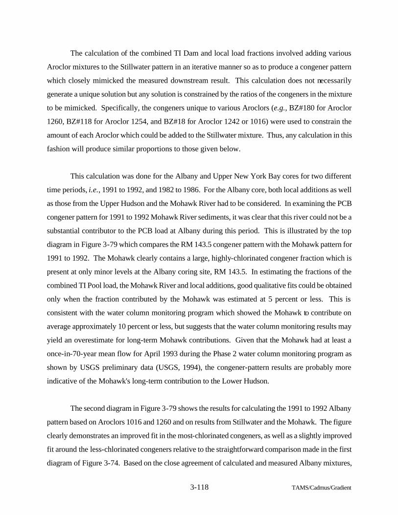
3-118 TAMS/Cadmus/Gradient
The calculation of the combined TI Dam and local load fractions involved adding various
Aroclor mixtures to the Stillwater pattern in an iterative manner so as to produce a congener pattern
which closely mimicked the measured downstream result. This calculation does not necessarily
generate a unique solution but any solution is constrained by the ratios of the congeners in the mixture
to be mimicked. Specifically, the congeners unique to various Aroclors (e.g., BZ#180 for Aroclor
1260, BZ#118 for Aroclor 1254, and BZ#18 for Aroclor 1242 or 1016) were used to constrain the
amount of each Aroclor which could be added to the Stillwater mixture. Thus, any calculation in this
fashion will produce similar proportions to those given below.
This calculation was done for the Albany and Upper New York Bay cores for two different
time periods, i.e., 1991 to 1992, and 1982 to 1986. For the Albany core, both local additions as well
as those from the Upper Hudson and the Mohawk River had to be considered. In examining the PCB
congener pattern for 1991 to 1992 Mohawk River sediments, it was clear that this river could not be a
substantial contributor to the PCB load at Albany during this period. This is illustrated by the top
diagram in Figure 3-79 which compares the RM 143.5 congener pattern with the Mohawk pattern for
1991 to 1992. The Mohawk clearly contains a large, highly-chlorinated congener fraction which is
present at only minor levels at the Albany coring site, RM 143.5. In estimating the fractions of the
combined TI Pool load, the Mohawk River and local additions, good qualitative fits could be obtained
only when the fraction contributed by the Mohawk was estimated at 5 percent or less. This is
consistent with the water column monitoring program which showed the Mohawk to contribute on
average approximately 10 percent or less, but suggests that the water column monitoring results may
yield an overestimate for long-term Mohawk contributions. Given that the Mohawk had at least a
once-in-70-year mean flow for April 1993 during the Phase 2 water column monitoring program as
shown by USGS preliminary data (USGS, 1994), the congener-pattern results are probably more
indicative of the Mohawk's long-term contribution to the Lower Hudson.
The second diagram in Figure 3-79 shows the results for calculating the 1991 to 1992 Albany
pattern based on Aroclors 1016 and 1260 and on results from Stillwater and the Mohawk. The figure
clearly demonstrates an improved fit in the most-chlorinated congeners, as well as a slightly improved
fit around the less-chlorinated congeners relative to the straightforward comparison made in the first
diagram of Figure 3-74. Based on the close agreement of calculated and measured Albany mixtures,
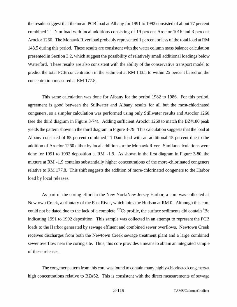
3-119 TAMS/Cadmus/Gradient
the results suggest that the mean PCB load at Albany for 1991 to 1992 consisted of about 77 percent
combined TI Dam load with local additions consisting of 19 percent Aroclor 1016 and 3 percent
Aroclor 1260. The Mohawk River load probably represented 1 percent or less of the total load at RM
143.5 during this period. These results are consistent with the water column mass balance calculation
presented in Section 3.2, which suggest the possibility of relatively small additional loadings below
Waterford. These results are also consistent with the ability of the conservative transport model to
predict the total PCB concentration in the sediment at RM 143.5 to within 25 percent based on the
concentration measured at RM 177.8.
This same calculation was done for Albany for the period 1982 to 1986. For this period,
agreement is good between the Stillwater and Albany results for all but the most-chlorinated
congeners, so a simpler calculation was performed using only Stillwater results and Aroclor 1260
(see the third diagram in Figure 3-74). Adding sufficient Aroclor 1260 to match the BZ#180 peak
yields the pattern shown in the third diagram in Figure 3-79. This calculation suggests that the load at
Albany consisted of 85 percent combined TI Dam load with an additional 15 percent due to the
addition of Aroclor 1260 either by local additions or the Mohawk River. Similar calculations were
done for 1991 to 1992 deposition at RM -1.9. As shown in the first diagram in Figure 3-80, the
mixture at RM -1.9 contains substantially higher concentrations of the more-chlorinated congeners
relative to RM 177.8. This shift suggests the addition of more-chlorinated congeners to the Harbor
load by local releases.
As part of the coring effort in the New York/New Jersey Harbor, a core was collected at
Newtown Creek, a tributary of the East River, which joins the Hudson at RM 0. Although this core
could not be dated due to the lack of a complete 137Cs profile, the surface sediments did contain 7Be
indicating 1991 to 1992 deposition. This sample was collected in an attempt to represent the PCB
loads to the Harbor generated by sewage effluent and combined sewer overflows. Newtown Creek
receives discharges from both the Newtown Creek sewage treatment plant and a large combined
sewer overflow near the coring site. Thus, this core provides a means to obtain an integrated sample
of these releases.
The congener pattern from this core was found to contain many highly-chlorinated congeners at
high concentrations relative to BZ#52. This is consistent with the direct measurements of sewage
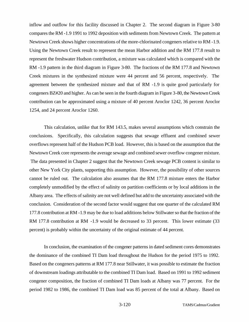
3-120 TAMS/Cadmus/Gradient
inflow and outflow for this facility discussed in Chapter 2. The second diagram in Figure 3-80
compares the RM -1.9 1991 to 1992 deposition with sediments from Newtown Creek. The pattern at
Newtown Creek shows higher concentrations of the more-chlorinated congeners relative to RM -1.9.
Using the Newtown Creek result to represent the mean Harbor addition and the RM 177.8 result to
represent the freshwater Hudson contribution, a mixture was calculated which is compared with the
RM -1.9 pattern in the third diagram in Figure 3-80. The fractions of the RM 177.8 and Newtown
Creek mixtures in the synthesized mixture were 44 percent and 56 percent, respectively. The
agreement between the synthesized mixture and that of RM -1.9 is quite good particularly for
congeners BZ#20 and higher. As can be seen in the fourth diagram in Figure 3-80, the Newtown Creek
contribution can be approximated using a mixture of 40 percent Aroclor 1242, 36 percent Aroclor
1254, and 24 percent Aroclor 1260.
This calculation, unlike that for RM 143.5, makes several assumptions which constrain the
conclusions. Specifically, this calculation suggests that sewage effluent and combined sewer
overflows represent half of the Hudson PCB load. However, this is based on the assumption that the
Newtown Creek core represents the average sewage and combined sewer overflow congener mixture.
The data presented in Chapter 2 suggest that the Newtown Creek sewage PCB content is similar to
other New York City plants, supporting this assumption. However, the possibility of other sources
cannot be ruled out. The calculation also assumes that the RM 177.8 mixture enters the Harbor
completely unmodified by the effect of salinity on partition coefficients or by local additions in the
Albany area. The effects of salinity are not well defined but add to the uncertainty associated with the
conclusion. Consideration of the second factor would suggest that one quarter of the calculated RM
177.8 contribution at RM -1.9 may be due to load additions below Stillwater so that the fraction of the
RM 177.8 contribution at RM -1.9 would be decreased to 33 percent. This lower estimate (33
percent) is probably within the uncertainty of the original estimate of 44 percent.
In conclusion, the examination of the congener patterns in dated sediment cores demonstrates
the dominance of the combined TI Dam load throughout the Hudson for the period 1975 to 1992.
Based on the congeners patterns at RM 177.8 near Stillwater, it was possible to estimate the fraction
of downstream loadings attributable to the combined TI Dam load. Based on 1991 to 1992 sediment
congener composition, the fraction of combined TI Dam loads at Albany was 77 percent. For the
period 1982 to 1986, the combined TI Dam load was 85 percent of the total at Albany. Based on
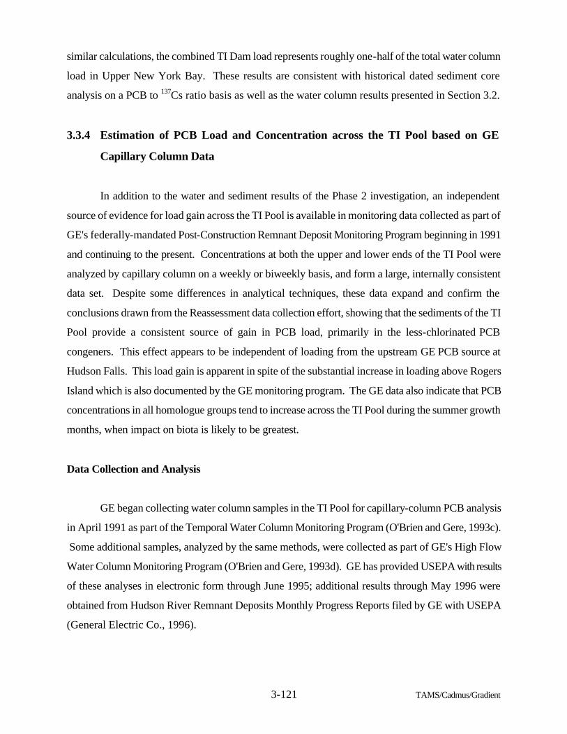
3-121 TAMS/Cadmus/Gradient
similar calculations, the combined TI Dam load represents roughly one-half of the total water column
load in Upper New York Bay. These results are consistent with historical dated sediment core
analysis on a PCB to 137Cs ratio basis as well as the water column results presented in Section 3.2.
3.3.4 Estimation of PCB Load and Concentration across the TI Pool based on GE
Capillary Column Data
In addition to the water and sediment results of the Phase 2 investigation, an independent
source of evidence for load gain across the TI Pool is available in monitoring data collected as part of
GE's federally-mandated Post-Construction Remnant Deposit Monitoring Program beginning in 1991
and continuing to the present. Concentrations at both the upper and lower ends of the TI Pool were
analyzed by capillary column on a weekly or biweekly basis, and form a large, internally consistent
data set. Despite some differences in analytical techniques, these data expand and confirm the
conclusions drawn from the Reassessment data collection effort, showing that the sediments of the TI
Pool provide a consistent source of gain in PCB load, primarily in the less-chlorinated PCB
congeners. This effect appears to be independent of loading from the upstream GE PCB source at
Hudson Falls. This load gain is apparent in spite of the substantial increase in loading above Rogers
Island which is also documented by the GE monitoring program. The GE data also indicate that PCB
concentrations in all homologue groups tend to increase across the TI Pool during the summer growth
months, when impact on biota is likely to be greatest.
Data Collection and Analysis
GE began collecting water column samples in the TI Pool for capillary-column PCB analysis
in April 1991 as part of the Temporal Water Column Monitoring Program (O'Brien and Gere, 1993c).
Some additional samples, analyzed by the same methods, were collected as part of GE's High Flow
Water Column Monitoring Program (O'Brien and Gere, 1993d). GE has provided USEPA with results
of these analyses in electronic form through June 1995; additional results through May 1996 were
obtained from Hudson River Remnant Deposits Monthly Progress Reports filed by GE with USEPA
(General Electric Co., 1996).
3-122 TAMS/Cadmus/Gradient
Stations sampled on a regular basis by GE include, among others, the Route 197 Bridge
(Rogers Island) at RM 194.6, main channel side, which is at the north end of the TI Pool (referred to
by GE as RM 194.2 due to differences in mapping references), and the western wing wall of the TI
Dam, at RM 188.5 which is at the south end of the TI Pool. Comparison of results at these stations
quantifies changes in PCB mass and concentration during flow through the TI Pool. For the period of
April 5, 1991 through May 29, 1996 there are 250 validated capillary-column results available for the
Rogers Island station, and 229 for the TI Dam station.
GE's analytical contractor, Northeast Analytical Laboratories (NEA) analyzed both total water
and filtered samples by capillary-column GC, and reported the data as total PCBs and percent
contribution by homologue group. Total concentrations were reported for every sample while
dissolved concentrations were not. Only the results for the total water samples are presented here.
NEA performed these analyses using their own protocol, NEA-608-CAP, which differs from the
analytical protocol used in the Reassessment and achieved resolution of fewer individual congeners.
The resulting chromatograms contain a number of co-eluting peaks containing more than one
homologue; thus homologue totals reported by NEA may differ from those obtained by the
TAMS/Cadmus/Gradient team. Coelution of dichlorobiphenyl congeners BZ#4 and BZ#10, which are
often significant in the Hudson River, is expected to result in a mis-estimation of the dichloro-
homologue total. In sum, the GE results may have some consistent differences from those obtained in
the Reassessment, but do provide an internally consistent basis for evaluating changes in load.
The NEA capillary-column analyses attained a nominal method detection limit (MDL) of 11
parts per trillion on total PCBs. Most samples used for this analysis were above that level. However,
the laboratory did report a qualified concentration for samples below the MDL in which PCBs were
detected. While these below-MDL values may be unreliable as individual measurements, they are
expected to be correct on average and were included in the analysis, rather than setting the below-
MDL values to an arbitrary value or zero.
3-123 TAMS/Cadmus/Gradient
Analysis of PCB Loads across the TI Pool
The GE PCB concentration data are discrete point-in-time (instantaneous) measurements. To
evaluate long-term trends on a mass-balance basis these are converted to estimates of total load
delivery. Concentration can be converted to load by multiplying the instantaneous concentration by
daily mean flow; however, load estimates must also be provided for days on which concentration was
not measured. To estimate monthly loads, the team used the monthly averaging estimator of Dolan et
al. (1981), which has been demonstrated by Preston et al.(1989) to provide relatively accurate results
estimates of load for analysis of samples obtained on a fixed time schedule. This estimator is:
where:
Lm is the load estimate for month m;
Nm is the number of days in month m;
qj is the daily mean flow on day j;
nm is the number of days on which PCB observations were made during month m; and
ci is a measured concentration within the month.
Simply put, the mean concentration observed during a month is multiplied by the sum of all daily flows
for that month, yielding, with correction for units, a load estimate in kg/month. Summation of flows
over an entire month will tend to dampen out any timing errors in flow which may result from this
procedure.
Flows for the calculation of load were taken from published and provisional USGS gauge data
for the Hudson River at Fort Edward (station number 01327750) (USGS, 1993a, 1993b, 1994a, and
1996), which is located just above the Rogers Island sampling station. Daily flows were available
through February 1996, and loads have been estimated through this month. There is no flow gauge at
TI Dam, and flow there was assumed to be 1.0515 times flow at Fort Edward, based on the ratio of
drainage basin areas.
∑∑n
c q = Lm
in
1=ij
N
1=jm
mm
(3-36)
3-124 TAMS/Cadmus/Gradient
Figure 3-81 shows estimated monthly loads of total PCBs at RM 194.6 (Rogers Island) and
RM 188.5 (TI Dam). The anomalously-high PCB observation of January 19, 1994 at RM 194.6 was
not included; this sample is noted as having been collected from shore due to ice cover, and
abnormally high TSS concentrations in the sample (19 mg/L) suggest that the sample was contaminated
by disturbance of near-shore sediment during collection. During most months, the load appears to be
somewhat higher at TI Dam. There is, however, considerable month-to-month variability. High loads
in April 1992 and April 1993 reflect high spring flows; under these conditions, low concentrations can
represent considerable mass transport. The high loads in September 1991 occurred in conjunction
with relatively low flows. On September 18, 1991 concentrations at RM 194.6 (Rogers Island) rose
to over 4000 ng/L, which was two orders of magnitude greater than the previous mean, as shown in
Figure 3-82. This represents the first documented activation of the GE Hudson Falls facility source
upstream. The impact of the upstream source on total load is again clear in 1992 and early 1993, then
tapers off. Finally, a high estimated load at RM 194.6 (Rogers Island) in January 1993 is due to a
single observation of 1086 ng/L total PCBs on January 14. Sampling did not capture this
concentration slug at RM 188.5, and it is possible that this sample could also represent disturbance of
contaminated sediment in the sampling procedure, although it is not annotated as having been collected
from shore.
Longer-term trends are more readily seen by looking at the cumulative sum of the loads.
Figure 3-83 compares the cumulative total PCB loads at RM 194.6 (Rogers Island) and RM 188.5 (TI
Dam), along with upstream loads at RM 197.6 (Fenimore Bridge). The lines consistently diverge,
indicating a steady gain in PCB load across the TI Pool, independent of the upstream source. This
load gain is apparent under all conditions, even under the large increases in the upstream source at
Hudson Falls. RM 197.6 measurements indicate that the load upstream of Hudson Falls is usually
insignificant. The total estimated gain in PCB load in the water column during passage through the TI
Pool over the period of observations is 998 kg, or 203 kg/yr, as shown in Table 3-21.
The change in load across the TI Pool varies dramatically with homologue group. Of the total
gain in PCB load, 90 percent is in the mono- through tri-chlorinated homologue groups. Figures 3-84
through 3-87 show the cumulative loads for mono-, di-, tri- and tetra-chlorinated biphenyl homologues
respectively. The mono-chlorinated homologues at TI Dam appear to have been derived almost
entirely from within the TI Pool, and the di-chlorinated homologues also show a strong gain. In
3-125 TAMS/Cadmus/Gradient
contrast, most of the tetra-chlorinated homologue load is already present at Rogers Island, with only a
slight gain measured at TI Dam. Similarly, only small gains in the other, more-chlorinated homologues
were observed.
A plot of the mean daily load (Figure 3-88) also shows an increase in loading rate, on average,
in the mono- through penta-chlorinated homologue groups, with strongest increases in the mono-
through tri-chlorinated homologues. Together with the cumulative load analysis, this indicates a
consistent gain in the less-chlorinated homologues during transit through the TI Pool. These
homologue groups contain PCB congeners which are anaerobic dechlorination endpoints and most
likely represent a flux of weathered PCBs from the TI Pool sediments as discussed in Section 3.2.
An alternative hypothesis for the increase in the mono- and di-chlorinated homologue loads is
that the load leaving the TI Pool represents the release of stored PCBs derived from the upstream
source which are then rapidly dechlorinated within the TI Pool. It does not, however, appear that the
bulk of load gain in the mono- and di-chlorinated congeners can be attributed to this process, for the
following reasons:
• There is a large and consistent gain in total PCB mass across the TI Pool;
• No corresponding reduction in the mass of the more-chlorinated congeners entering
the TI Pool has been detected which would account for the increase in mass of
dechlorination products;
• Dechlorination appears to be a significant process only under anaerobic
conditions, whereas the surface sediment layer in the TI Pool is typically aerobic.
Given evidence of low burial rates, there are no known mechanisms by which
massive dechlorination of PCBs loaded to the TI Pool from upstream could occur
over short time horizons.
Figures 3-89 through 3-93 display the estimated load gain on a month-by-month basis for total
PCBs and mono- through tetra-chlorinated homologues. These do not show any clear evidence of
storage and later release of upstream loads, i.e., nearly all months show a load gain across the pool.
Loads of mono- and di-chlorinated homologues are reduced during 1995 primarily because this was a
drought year, resulting in lower rates of mass transport. Total flows at Fort Edward for April though
3-126 TAMS/Cadmus/Gradient
August 1995 were only 30 percent of those during the same period in 1994. It is of interest to compare
the load gains observed in the April through August 1991 period, which is prior to the onset of recent
major releases by the GE Hudson Falls facility, to those in June through December 1993, when the GE
Hudson Falls source was again largely inactive. All homologues show a similar pattern in which the
June to December 1993 loads are elevated above those of April to August 1991. The relative change
in load is smallest in the monochlorobiphenyl fraction and increases with increasing level of
chlorination. This could in part reflect an increase in surface sediment contamination since 1991
which would tend to affect the homologue groups in proportion to the upstream source, i.e., principally
trichloro- and tetrachloro-homologues. Flows, however, were about 10 percent greater in the summer
of 1993 than in the summer of 1991, and substantially higher during the spring, with the April 1993
total flow at Fort Edward more than twice that of April 1991. Larger gains across the TI Pool in 1993
may thus be attributable primarily to greater erosive power, porewater displacement and transport
capacity in that year. These factors and their impacts on the water column PCB inventory are
discussed in Section 3.2.
Changes in Water Column PCB Concentration across the TI Pool
The GE data can also be used to examine changes in water column concentrations across the TI
Pool. First, in accordance with the load analysis, there is a significant change in the PCB homologue
composition, as shown in Figure 3-94. At RM 194.6 (Rogers Island), the mono-chlorinated
homologue group accounts for much less than 1 percent of the total PCB concentration, while the di-
chlorinated group accounts for a little less than 11 percent. At RM 188.5 (TI Dam), the mono-
chlorinated group has increased to 11 percent of the total, and the di-chlorinated group to nearly 18
percent. While the tri-chlorinated group has declined as a percent of the total, it has increased its
importance in relation to the more-chlorinated homologues. This is generally consistent with the
Phase 2 investigation results, although the Phase 2 results indicate an even greater shift to the less-
chlorinated homologue groups.
Summer water column concentrations are of particular importance to bioaccumulation.
Examination of concentrations for the June through August period indicates that a consistent gain in
concentrations through at least the tetra-chlorinated homologue group occurs during summer low-flow
transit through the TI Pool. Figures 3-95 through 3-99 display mean concentrations at Rogers Island
and TI Dam for the summers of 1991, 1992, 1993, 1994, and 1995. The gain in lower-chlorinated
homologue groups across the TI Pool is evident in all six years, although total concentrations change.
3-127 TAMS/Cadmus/Gradient
The differences between the years are also significant; the 1991 data represent conditions before most
of the major releases from the GE Hudson Falls facility occurred. In contrast, substantial PCB loading
from the Hudson Falls facility did occur in summer 1992, and the mean concentrations are higher,
although still showing a gain across the Pool in the mono- through tetra-chlorinated congeners. In
summer 1993 and subsequent years, the Hudson Falls source again appears to have been relatively
inactive. The homologue pattern of summer mean concentrations in this year is similar to 1991, but
with somewhat higher concentrations of mono- and di-chlorinated homologues at TI Dam. In summer
1994 and 1995, homologue concentrations were similar to summer 1991, except for an apparent
increase in mono- and di-chlorinated congener concentrations relative to 1991.
In conclusion, the GE monitoring results define both the scale of the recent Hudson Falls
facility PCB releases and the load gain across the TI Pool for the period April 1991 to February 1996.
The load gain is consistent with that found in the Phase 2 results discussed previously. In particular,
both the GE and the Phase 2 results indicate that, for 1993, summer water column levels and loads are
principally derived from the TI Pool. As illustrated in Figure 3-97, the mean summer water column
inventory at the TI dam is three to four times greater than that at Rogers Island, indicating that two-
thirds to three-quarters of the water column PCB inventory at TI Dam is derived from the Pool. Based
on the interpretation in Section 3.2, all points downstream are affected in a similar fashion. For
summer 1991 conditions, approximately half of the water column inventory at TI Dam was derived
from the Pool. Thus, the GE data provide a longer-term measure of the importance of the TI Pool to
Hudson River water column PCB levels.
3.3.5 Estimated Historical Water Column Loadings Based on USGS Measurements
The measurement of water column PCB levels by the USGS represents one of the largest data
sets of its kind for the Hudson River. Due to analytical and sampling limitations, these data can be
used to develop only approximate estimates of water column PCB load, but still provide a useful
indication of historical trends in loading. This section presents an analysis of the historical water
column loading data, covering the period 1977 through 1994, using two different statistical techniques.
In the Phase 1 Report (USEPA, 1991), Table B.4-4 provides estimates of annual PCB load in
the Hudson River derived from USGS observations. The estimates contained in that table have now
3-128 TAMS/Cadmus/Gradient
been revised using additional data and a refined methodology for load estimation has been developed.
The present analysis confirms and expands the previously reported results. The Phase 1 Report
provided load estimates through calendar year 1989. New data have been obtained through the end
of 1994 (USGS, 1993b and 1994c). Some additional data have also been obtained for earlier years,
primarily because USGS-reported Aroclor values have been obtained in addition to total PCB
estimates.
The calculation methods differ from those used for the Phase 1 estimates in several respects.
First, daily mean flows have been used for estimation rather than instantaneous discharge values.
(Flows at Schuylerville were estimated from Fort Edward data.) Where multiple concentration
measurements are available for the same day, these have been averaged. Nondetects on total PCB
concentrations were set to one-half the nominal detection limit. Nondetects in individual Aroclor data
were set to zero in calculating totals from sums; but if all Aroclor concentrations were reported non-
detect, and a total PCB concentration was not reported by USGS, the total concentration was set to
one-half the nominal detection limit for totals in that time period.
The "corrected mean" method used for the Phase 1 Report was an ad hoc method designed to
help avoid the problem of bias in sampling. However, its statistical properties have not been
established, and the method has not been tested on other data sets, which reduces defensibility of the
resulting estimates. Preston et al.(1991) investigated the performance of 24 different methods
proposed for estimating mass loads in streams from limited concentration observations. These
methods include various types of averaging, ratio and regression estimators, applied with and without
stratification, and under systematic and event-focused sampling, with evaluation of error and bias.
Stratification is a process of data separation into subsets or bins, where each bin is characterized, as
defined here, by a narrow range of values. They considered load estimation for total phosphorus, zinc,
ammonia, copper, iron, Aroclor 1242 and Aroclor 1260 in the Grand and Saginaw Rivers,
representing a variety of flow-concentration patterns. Preston et al. concluded that no single estimator
could be determined a priori superior for a given situation. However, certain estimators performed
relatively well for all test situations, including estimation of Aroclor loads in the Saginaw River. In
particular, ratio estimators (adapted from sampling statistics) were recommended as robust to sources
of bias inherent in flow-concentration relationships, and, when stratified by flow, were also resistant
to bias in event sampling. TAMS/Cadmus/Gradient therefore applied a stratified version of the ratio
3-129 TAMS/Cadmus/Gradient
estimator developed by Cochran (1977). Table 3-22 displays the stratification criteria; resulting load
estimates are shown in Table 3-23.
Averaging methods have been more commonly applied to load estimation than ratio estimators,
and some averaging methods also performed well in the tests conducted by Preston et al. The monthly
and seasonal averaging methods of Dolan et al. (1981), which use average observed concentrations
with the complete record of daily flows, were generally precise, i.e., having low variability, but in
some cases showed greater bias than ratio estimators. For comparison, Table 3-23 also shows the
results of applying a seasonal averaging method; data were insufficient to apply monthly averaging.
The results of applying this estimator are generally in close agreement with the ratio estimator results.
The ratio estimator of Cochran (1977), calculated over k individual strata, is:
where:
L is the total annual estimate of load;
l is the average load on days where measurements were taken in the stratum;
q is the average flow on days where measurements were taken in the stratum; and
Q is the sum of all daily flows falling within that stratum over the course of the year.
The asymptotic estimate of the variance for the ratio estimator is given by:
where:
s�lh is the sample variance of load in stratum h;
s�qh is the sample variance of flow in stratum h;
Rh is the ratio of load to flow in stratum h; and
( )Q q/l = L hhh
k
1=h∑ (3-37)
( )CV R 2 - s R + s n
)n-N( N V lqhh2qh
2h
2lh
h
hhhk
1=h∑≈ (3-38)
3-130 TAMS/Cadmus/Gradient
CVlqh is the covariance between load and flow in stratum h.
The averaging estimator of load presented by Dolan et al. (1981) computes the mean
concentration observed during a given time period and then applies this mean to the complete series of
daily flows. This approach has been demonstrated to be much more reliable than estimates computed
by averaging individual load estimates, since the latter approach ignores the information present in the
flow values for days on which concentrations were not measured. The estimator is given by:
where:
m is season;
j is day within season;
Nh is the total number of days within the season;
nh is the number of days within the season for which concentration observations are
available; and
cijh are the individual concentration measurements.
Essentially, this method determines the average concentration within a season and then applies this
average over the complete series of measured flows for that season. Averaging estimators are
typically not stratified.
The four strata used for the ratio estimator were based on visual examination of sediment
rating curves at the USGS monitoring stations with breakpoints between strata summarized in Table 3-
22. The lower breakpoint approximately defines the low-flow regime in which concentrations appear
to show an inverse relation to flow. The breakpoint between the second and third strata is designed to
coincide approximately with the break between non-scouring and scouring regimes of 600 m3/s, or
21,000 cfs, at the Waterford gauge, proposed by Schroeder and Barnes (1983). Finally, the upper
breakpoint serves to address extreme high-flow events. In various cases, no samples were available
in a given year within one of the strata, usually one of the two high-flow strata. In such cases the
∑∑∑n
c q = Lh
ijhn
1=ijh
N
1=j
4
1=m
hh
(3-39)
3-131 TAMS/Cadmus/Gradient
degree of stratification was reduced from four to three, as needed to account for all daily flows within
the year.
The resulting estimates of load from the ratio and averaging methods are generally in
agreement, with the averaging estimates within two standard deviations of the ratio estimates. The
load estimates are also similar to the Phase 1 results, but reflect use of a different methodology and
increased sample size.
Station-by-station comparisons of load estimates are shown in Figure 3-100 for the ratio
estimator, and in Figure 3-101 for the averaging estimator. Loads upstream of RM 194.6 at Rogers
Island generally declined from 1983 to 1991, then increased in 1992, reflecting releases from the
upstream source at the GE Hudson Falls facility. Loads upstream of RM 194.6 at Rogers Island then
declined in 1993 and 1994, with 1994 loads being the lowest for any year estimated. 1994 loads at
the downstream stations also declined, but are similar to estimates for 1988-1991 (see Figure 3-101).
As with the load-estimation results reported in Phase 1, there is no obvious and consistent gain in
load downstream of Rogers Island after 1984 although results vary considerably from year to year.
The relatively high level of uncertainty in the estimates, however, may obscure all but gross trends.
In general, the analysis of the USGS data confirms the loading trends seen in the dated
sediment cores presented in Subsection 3.3.3, i.e., a relatively steady decrease up to the mid-1980s
followed by a plateau in the loading from the Upper Hudson. The absence of an obvious increase in
load between Rogers Island and Waterford conflicts directly with the Phase 2 water column
monitoring results which show a substantial load gain across the TI Pool throughout the monitoring
period. It is likely, however, that this discrepancy is largely due to differences in the analytical
methods used. Specifically, the USGS data are reported with relatively high detection limits and do
not accurately reflect the monochloro- and dichlorobiphenyl fraction of the water column load, as
discussed by Bush et al. (1987). As discussed in Section 3.2, these represent substantial portions of
the water column load, and principally originate below Rogers Island in the TI Pool. Based on the
results discussed in Section 3.2 and Subsection 3.3.4, it is evident that much of the more-chlorinated
congener loading originates above Rogers Island while the less-chlorinated congeners originate in the
TI Pool. Since the USGS data are analytically focused toward the more-chlorinated congeners, these
results are considered to be consistent with the Phase 2 results, given the analytical uncertainties.
3-132 TAMS/Cadmus/Gradient
In conclusion, the USGS results show a decline in Upper Hudson PCB loading from the late
1970s to roughly 1984 followed by a relatively stable load, largely originating above RM 194.6 at
Rogers Island. High loads estimated for 1992 reflect the recent releases from the GE Hudson Falls
facility. The USGS results do not accurately represent the load of less-chlorinated PCB congeners in
the water column, and so can only be used to track the more-chlorinated congeners over time. The
results suggest that the majority of the heavier congeners in the water column have originated above
Rogers Island since about 1984.
3.3.6 Conclusions Concerning Historical Water Column Transport
Section 3.3 of the Phase 2 report examines historical water column PCB transport based on
several different data sets. Each of these data sets provides an independent estimate of water column
loads at similar river locations. In general, the conclusions drawn from each data set are comparable
although there are some differences.
Based on the examination of Phase 2 suspended matter and 7Be-bearing sediments, several
important results were obtained which support the use of dated sediment cores as records of the water
column. A close agreement was found between the congener patterns of local suspended-matter
measurements and the associated surface sediments. Good agreement was also found between the
range of the total PCB concentrations on suspended matter and that in surface sediments. These results
demonstrate that 7Be-bearing sediments record the suspended-matter conditions from which they were
derived. By inference, in cores from locations which are shown to steadily accumulate sediment, the
suspended- matter patterns are continually recorded over time. The surface-sediment congener pattern
most closely agreed with spring suspended matter, as anticipated. This suggests that the dated
sediment cores integrate the water column transport in proportion to the suspended-matter load. Thus,
the dated sediment core results are most useful in documenting major suspended-matter transport
events. Given the importance of the spring-runoff event to PCB transport, the cores provide an
excellent means to monitor loadings on a long-term basis. Finally, the agreement between suspended-
matter sample PCB congener patterns within each transect is consistent with the agreement seen across
the surface-sediment PCB congener patterns. This result strongly suggests that suspended-matter PCB
transport occurs such that the PCB homologue distribution is preserved and that there are no
substantive additional sources in the freshwater region of the Upper and Lower Hudson.
3-133 TAMS/Cadmus/Gradient
The dated sediment cores provide two bases on which to examine the historical PCB loading
in the Hudson. The first basis is the sediment total PCB levels. These data were examined for 14
dated sediment cores from the Upper and Lower Hudson as well as the major tributaries. The
historical trends from 1975 to 1992 show a continual decrease in PCBs to the early 1980s followed by
a PCB concentration plateau which extends almost to the time of core collection in 1992. These
results document the absence of any major PCB releases by the GE Hudson Falls facility or any other
source for the period 1983 to 1990 on the scale of the 1991 and 1992 GE releases. The core results
also document the absence of significant sources to the Hudson upstream of the GE Hudson Falls
facility. A simple model of PCB transport assuming conservative transport between coring locations
was capable of explaining the general trend in sediment levels along the entire Hudson for each of four
time intervals between 1975 and 1992. The model corrected only for dilution by tributary flow and
accounted for different sediment deposition rates by normalizing for 137Cs. The results showed that
below RM 177.8 near Stillwater, PCB transport is largely conservative with no substantial losses or
gains as far downstream as RM 42.3, the northern end of the New York/New Jersey Harbor. This
result was consistent over the entire 17-year period examined and demonstrated the dominance of the
combined TI Dam load to the freshwater Hudson. The core results also appeared consistent with the
GE-documented increase in PCB loadings from the area upstream of RM 194.6 at Rogers Island,
although the uncertainties in the coring results were too great to confirm this trend.
Examination of PCB congener patterns yielded similar results concerning the importance of the
GE PCB loads in the freshwater Hudson. The results indicated that the suspended-matter PCB fraction
in the combined TI Dam load for 1991 to 1992 was roughly comprised of 82 percent Aroclor 1242, 16
percent Aroclor 1254 and 2 percent Aroclor 1260, based on the surface sediment congener pattern at
RM 177.8. The congener composition of suspended matter collected at RM 194.6 in April 1993
suggested the presence of these three Aroclors as well, although the fractions of Aroclors 1254 and
1260 were about one-third of those in the 1991 to 1992 sediments. The fractions of the latter two
Aroclors were unexpected based on reported GE PCB usage over time and suggest that the current
releases are somehow a mixture of all historical usage at the facilities. In particular, there is no
reported usage of Aroclor 1260 by GE although it is clearly present in the water column load derived
from their facilities.
3-134 TAMS/Cadmus/Gradient
The congener patterns themselves showed good consistency downstream of the TI Dam at RM
188.5. Using five sediment cores from RM 177.8 near Stillwater to RM -1.9 in Upper New York Bay,
the importance of the RM 177.8 pattern, and, therefore, the combined TI Dam load throughout the
Hudson, was apparent. An examination of congener patterns at RM 177.8 near Stillwater over time
was used to document the combined TI Dam load history from 1975 to 1992. The patterns showed
only minimal variability over time, with a gradual shift to more-chlorinated congeners from the period
1975 through 1981 to the period of 1982 through 1986, suggesting the presence of additional Aroclor
1254 in the more recent period. After 1982, the congener pattern appears very consistent over time.
A similar change in the PCB congener distribution over time was also observed in downstream cores,
supporting the conclusions of the suspended-matter/surface-sediment comparison.
The congener patterns in downstream cores were relatively consistent with those near
Stillwater. The minor differences were used to estimate the amount of additional loading which
occurred between RM 177.8 and two downstream locations, i.e., RM 143.5 near Albany and RM -1.9
in Upper New York Bay. Additional loadings were calculated for 1982 to 1986 and 1991 to 1992
conditions. At Albany, 1991 to 1992 deposition was estimated to consist primarily of the combined
TI Dam load with possibly 22 percent derived from local loadings. The remaining 5 percent was
derived from the Mohawk River. For 1982 to 1986, the combined TI Dam load represented 85
percent of the load at RM 143.5. To some extent weathering of the PCB homologue pattern in the
water column or soon after deposition may be responsible for the apparent local loadings since loss of
lighter congeners would give the appearance of an additional local PCB load. This would be more
consistent with the result obtained from the total PCB 137Cs analysis which indicated the absence of
substantive PCB loads in the freshwater Hudson other than those from the Upper Hudson. In Upper
New York Bay, the combined TI Dam loading appeared to represent roughly one-half of the 1991 to
1992 Harbor load based solely on sediment congener pattern, consistent with the findings of Bopp and
Simpson for 1982 to 1986 time period (Bopp and Simpson, 1989)
The GE monitoring data cover only a relatively short period of time, i.e., April 1991 to May
1996, as compared to the dated sediment cores. However, the results obtained document the large
loads originating upstream of RM 194.6 over this time period, attributed by GE to the GE Hudson
Falls facility. The GE data also support and extend the general findings of Section 3.2, i.e., that the
Thompson Island Pool represents a major source of PCBs to the water column with greatest load
3-135 TAMS/Cadmus/Gradient
increases in the mono- through trichlorinated homologues. This gain in lower-chlorinated homologue
groups across the TI Pool is evident throughout the 1991 to 1996 period. Increased concentrations of
mono- and dichlorinated homologues were evident in the years following the 1992 releases from the
GE Hudson Falls facility relative to 1991 concentrations.
Table 3-23 compares the PCB water column loads at Rogers Island and the TI Pool for 1993
based on Phase 2, GE and USGS water column data. Evident in both the Phase 2 and GE data is the
importance of the TI Pool source. Both data sets document the scale and the characteristic shift of the
PCB load to less-chlorinated congeners across the TI Pool. The table also shows the good agreement
between estimates generated by Phase 2 and GE data sets for total PCB levels.
The USGS data set provides the longest-term water column monitoring record. These data
show the same general temporal record as the dated sediment cores for the period 1975 to 1992, i.e., a
large decrease in the PCB loading during the period 1975 to the mid-1980s, followed by a plateau in
the loading from the Upper Hudson loads up to 1991. Like the core data, the USGS data do not show
evidence for large releases originating upstream of RM 194.6 at Rogers Island prior to 1992. In
contrast to the Phase 2, and GE water column monitoring results, the USGS data do not indicate a
substantial load gain across the TI Pool. This is likely due to the analytical method used. Specifically,
the USGS data do not accurately reflect the mono- and di-chlorinated homologue fractions of the water
column load, since they are focused on Aroclor standards which contain little of these homologues.
Based on the Phase 2 data presented in Section 3.2, the less-chlorinated congeners represent a
significant fraction (on the order of 50 percent) of the TI Pool load. Thus, considering the analytical
limitations of the USGS methodology, the USGS results are not inconsistent with the Phase 2 and GE
data, both of which suggest that less-chlorinated congeners represent a substantial portion of the TI
Pool source while the more heavily-chlorinated congeners appear to originate upstream of the TI Pool.
Overall, this examination has documented the importance of the combined TI Dam load to the
entire Hudson River. The examination of GE data confirmed the finding of the Phase 2 water column
investigation showing the dominance of the TI Pool source to water column loads during at least 11 of
12 months of the year, along with its characteristic less-chlorinated-congener composition. The GE
data also show the TI Pool load continuing up to the present time. The USGS results agree with the
dated sediment cores concerning the trend of PCB loading with time and the absence of significant
3-136 TAMS/Cadmus/Gradient
loadings from the GE Hudson Falls facility before 1991. The examination of dated sediment cores
documents the history of the combined TI Dam load and its long-term dominance of the water column
PCB inventory in the Lower Hudson. The core results examined on a mass basis also show PCB
transport to be largely conservative from RM 177.8 to RM 88.5 and possibly to RM 43.2. The
examination of congener composition in the cores yielded additional evidence supporting this
conclusion as well as evidence on the relative scale of the PCB load from the Mohawk River and
other sources below the TI Dam.
3.4 Integration of Water Column Monitoring Results
In the previous sections of Chapter 3, various studies and analyses are presented which
represent different aspects of water column PCB transport in the Hudson. Each examination provides
a unique and essentially independent perspective on water column PCB transport phenomena in the
Hudson. In this section, the results of these analyses are compiled to provide an integrated
interpretation of water column PCB transport. Specifically, this section summarizes the overall
findings and cites the supporting evidence for the various conclusions among all the analyses
presented previously. A listing of the major conclusions is provided in Section 3.6 following a
discussion of PCB loadings to the Lower Hudson in Section 3.5.
Of particular interest in this report are the conclusions regarding PCB loadings from the TI
Pool sediments. This section summarizes the evidence for the nature and size of this loading based on
three independent measurement programs. The evidence strongly supports the conclusion that TI Pool
sediments currently represent approximately 65 percent of the total PCB load to the water column and
that loadings from the Bakers Falls-TI Pool area represent the single largest PCB source to the entire
freshwater Hudson.
3-137 TAMS/Cadmus/Gradient
3.4.1 Monitoring Techniques and PCB Equilibrium
This section summarizes the important conclusions concerning the techniques applied in
sampling. These sampling achievements support the geochemical discussions that follow. For the
water column monitoring programs, a satisfactory level of sampling precision was obtained whereby
loading differences between monitoring stations greater than 20 percent can be considered significant.
The results of the short-term measurement of water- column conditions, i.e., transects and flow-
averaged sampling, are well supported by the dated sediment-core results. Surface-sediment PCB
congener patterns match suspended-matter PCB patterns, giving credence to the extrapolation of the
water column monitoring results to longer-term conditions. This result also confirms the link between
dateable sediment cores and the water column. This link between water column samples and dateable
sediment cores was established over most of the freshwater Hudson (more than 100 miles) and serves
to strengthen the conclusions drawn from either program. The sediment coring program obtained 14
datable cores from 12 locations covering more than 200 river miles and three major tributaries. This
data set was used to examine historical water column PCB transport over this entire distance back to
1975.
In addition to the success of the Phase 2 water column monitoring programs, the investigation
was also able to examine the nature of PCB sediment-water partitioning in the Hudson. Based on the
wide range of water column conditions sampled, an empirical relationship among the partition
coefficient, the concentration of suspended organic matter (particulate organic carbon), and the water
temperature was developed for each target congener. This relationship is capable of predicting in situ
congener-specific partition coefficients to within "50 percent based solely on these variables when
equilibrium conditions are anticipated. Further analysis of PCB partitioning strongly suggested that
the PCB distribution at Rogers Island was not in equilibrium whereas points downstream of Rogers
Island appear to be close to equilibrium conditions. Thus, suspended matter-water equilibrium can be
assumed when interpreting sampling results at the TI Dam and below. This conclusion aids the current
interpretation as well as the Phase 2 modeling effort. Specifically, this conclusion greatly increases
the usability of the dated sediment cores since it can be assumed that the PCB levels and patterns in the
sediments were in equilibrium with the water column before deposition. Therefore, variations in
sediment-core PCB concentrations directly reflect variations in water column PCB levels.
3-138 TAMS/Cadmus/Gradient
This conclusion is supported by the PCB equilibration study and by the special set of
circumstances surrounding Transect 3 in March 1993. The PCB equilibration study showed no
substantive shift in partition coefficients in samples held for four days before filtering relative to those
samples collected and filtered within four hours of collection, implying that an effective sediment-
water PCB equilibrium had been established prior to collection. It should be noted that four days is
the approximate transit time for water between Rogers Island and Waterford during much of the year
and thus represents the standard amount of time available to establish equilibrium in the water column.
The third transect provides some additional information on the speed of equilibration. During
this transect, water column concentrations between Stillwater and Waterford increased roughly
fifteen-fold within a 24-hour period as the result of Hudson River sediment scour induced by the
Hoosic River. In spite of the speed of this change, PCB partition coefficients changed only slightly
relative to upstream conditions. The implication of this result is that sediment-water PCB equilibrium
is established within 24 hours of the addition of new material to the water column.
The finding that Rogers Island is out of equilibrium relative to downstream locations is
consistent with its proximity to the GE Hudson Falls facility whose loading is monitored at Rogers
Island. For this investigation, the transit time between Hudson Falls and Rogers Island was always
less than six hours and frequently less than four hours. It should be noted, however, that the difference
in Rogers Island conditions relative to locations downstream may also be the result of the form of PCB
release from the GE Hudson Falls facility. GE has found evidence to indicate that some of the PCB
load from this facility enters the river as a PCB-bearing oil (O�Brien & Gere, 1994a), which may
effect the time needed for equilibrium or the number of phases involved in equilibrium.
3-139 TAMS/Cadmus/Gradient
3.4.2 Loadings Upstream of the TI Pool
Before examining the loadings from the TI Pool, it is first necessary to examine the loading
originating upstream of the Pool, specifically the water column loads at the Fenimore Bridge (RM
197.4) and at Rogers Island (RM 194.5). Samples from these locations can be used to represent the
background loading from the Upper Hudson and from the GE facilities and remnant deposit area,
respectively. Background conditions at the Fenimore Bridge have been monitored as part of the Phase
2 investigation, as well as by GE as part of its Post-Construction Remnant Deposits Monitoring
Program. Both programs show the loading at RM 197.2 to be much less than PCB loading originating
between RM 197.2 and the TI Dam.
On average, the Phase 2 results indicate the average background flux to be less than 0.03
kg/day (0.78 kg/month) or 1.4 percent of the downstream loadings at TI Dam. The homologue pattern
was found to be highly variable with more-chlorinated congeners representing most of the mass, unlike
the downstream loads (Figures 3-38, 3-40, 3-43, and 3-47 show the homologue patterns for the
downstream loads). The data from General Electric for June 1991 to February 1996 yield a flow-
weighted average background flux of 0.20 kg/day (5.9 kg/month). The GE estimate is constructed
using values as reported including those below their reported detection limit or as one-half the
detection limit when the data are simply reported as non-detect. The higher load estimate for GE is
largely attributed to their higher detection limit relative to the Phase 2 study which limits the
usefulness of the GE data set in estimating background loads. For example, during the Phase 2 study
period, the mean GE load was 0.14 kg/day relative to the Phase 2 reported load of 0.03 kg/day. Of
particular note are two singular concentrations reported by GE for November 2, 1995 and December
27, 1995 at the Fenimore Bridge. The concentrations were nearly 100 times greater than any previous
or subsequent measurement. The reason for these two high values is unknown but they are inconsistent
with subsequent downstream concentrations and may be the results of construction activities at the
Bakers Falls Dam. Excluding these two high values, the mean loading at Fenimore Bridge for April
1991 to February 1996 drops to 0.13 kg/day. Utilizing the GE data for the post-Phase 2 monitoring
period, October 1993 to February 1996, an upper bound background load estimate of 15 percent of the
TI Dam load is obtained.
3-140 TAMS/Cadmus/Gradient
Both the Phase 2 and GE estimates are considered upper bounds on the background PCB flux at
RM 197.2 due to analytical limitations, particularly in the case of the GE data. Water column
concentrations at this location are very close to the analytical quantitation levels and thus measurement
uncertainty and potential blank contamination may serve to raise the measured values relative to actual
conditions.
These results are supported by the dated sediment core results for RM 202.9 near Glens Falls
and RM 188.5 in the TI Pool. The core at RM 202.9 is considered to represent background
suspended-matter loads from the Upper Hudson. The 137Cs-normalized PCB concentrations for this
location were 200 times lower than those at RM 188.5 for 1991 to 1992 and 800 times lower for 1975
to 1981. Thus all three data sets support the conclusion that the annual PCB loading upstream of the
Fenimore Bridge at RM 197.2 is small (less than 1.4 percent based on Phase 2 data) relative to
downstream loads for 1993. Based on the dated sediment cores, this conclusion can be extended back
to at least 1975.
The second and more significant loading originates between the Fenimore Bridge and the
northern tip of Rogers Island at RM 194.6 (or 194.3 for GE monitoring). This three-mile reach
includes the outfalls from both the GE Hudson Falls facility and the GE Fort Edward facility, as well
as the remnant deposits. Both TAMS/Cadmus/Gradient and GE have collected samples within this
reach as well as at either end. Based on their results, GE concludes that the loading at Rogers Island
originates almost exclusively at the GE Hudson Falls facility (O'Brien & Gere, 1994b). This
conclusion is based largely on the similarity of the congener patterns at two monitoring stations in this
reach.
The Phase 2 results, which involve monitoring at the Fenimore Bridge (background
conditions), at RM 195.5 near Remnant Deposit 2, and farther downstream at Rogers Island, confirm
the GE measurements; in particular, the concentration and loading at Rogers Island are nearly always
greater than those at RM 195.5 in spite of the upstream location's proximity to the GE Hudson Falls
facility. In addition, like the GE data, the congener pattern at Rogers Island is frequently the same as
that found at RM 195.5.
3-141 TAMS/Cadmus/Gradient
These results are consistent with GE's conclusion concerning the origin of loads in this reach
but do not prove their conclusion. However, this conclusion is not a necessary condition for the
subsequent analysis of TI Pool loadings. It is simply sufficient to establish the nature and scale of the
loadings at Rogers Island so that loads originating downstream in the TI Pool can be differentiated
from the upstream contributions. To this end, the Phase 2 data provide the most detailed information
on water column PCB conditions for the Phase 2 investigation period. The GE results provide less
detailed information over a longer period, i.e., April 1991 to May 1996.
Figure 3-102 shows the similarity of the results obtained at Rogers Island in March 1993 for
the Phase 2 and GE monitoring programs. Both analyses show the load to consist largely of tri-
chlorinated and tetra-chlorinated congeners, suggesting an Aroclor 1242-like source. There is also the
noticeable absence of significant levels of dechlorination products, specifically mono-chlorinated and
di-chlorinated congeners. The loading estimates given in the figure are based on the respective data
sets and are considered to be in generally good agreement given the different temporal monitoring
schemes, analytical techniques, and the variable nature of the Bakers Falls source at that time.
Both the Phase 2 and the GE data sets show the magnitude of the loading at Rogers Island to be
highly variable with no apparent temporal dependence. The highly variable loading is consistent with
the current understanding of the GE Hudson Falls facility PCB releases. These releases are believed
to occur as PCB-bearing oils which migrate through fractured bedrock to the Hudson. The nature of
the migration is not well understood but it does not appear to be continuous in nature. The largest
single loading increase during the Phase 2 investigations was found at Rogers Island, yielding 17
kg/day for Transect 4 in April 1993. Analysis of the congener content for the suspended matter for this
event suggested the presence of Aroclors 1242, 1254, and 1260 at 94 percent, 5 percent and 1 percent,
respectively, in the mixture. This result is confirmed by the dated sediment core at RM 177.8 near
Stillwater in which surface sediments were shown to contain a similar mixture in the ratio of 82:16:2,
respectively (see Figures 3-70 and 3-72). This result indicates that the load originating between
Bakers Falls and Rogers Island must contain all of these Aroclors.
The GE data for Rogers Island document the magnitude of the loadings over the period April
1991 to May 1996. Mean monthly load calculations are limited to April 1991 to February 1996 due to
the lack of available USGS mean monthly flow data. The GE data indicate that this loading was the
3-142 TAMS/Cadmus/Gradient
dominant source to the Upper Hudson during the period September 1991 to May 1993. They also
indicate that the loading represented a substantial increase over the preceding five-month period
(April to August, 1991). When this large release above Rogers Island was first discovered, it was
hoped that the dated sediment cores might reflect its impact on the River. However, due to the timing
of the major releases above RM 194.6 (September 1991 and June through October 1992) relative to
the collection of the sediment cores (September to October 1992), it is unclear as to whether the cores
should reflect this load increase.
The results for two downstream cores, at RM 177.4 near Stillwater and RM 143.5 near
Albany, indicate a small rise in surface sediment PCB concentrations relative to previous deposition.
Cores from both sites are characterized by particularly high deposition rates, i.e., 1.7 and 5.5 cm/yr,
respectively, which increases the resolution available to detect such load events. Both cores show a
relatively minor increase in 1991 to 1992 PCB levels normalized to 137Cs, approximately 10 to 25
percent higher than those over the previous three-year period. Cores collected subsequent to the Phase
2 investigation (Chillrad et al., 1996) yield increased surface concentrations at several Lower Hudson
Sites. These results as well as the small changes in the RM 177.8 and RM 143.5 cores suggests that
the increased loading at Rogers Island, while unquestionably important, was still small in comparison
to the water column loads of the 1970s and early 1980s. In particular, the results from Chillrad et al.
(1996) suggest that the loading may have been similar to the water column loads seen around 1984.
3.4.3 Loading from the TI Pool during 1993
Having established the validity of the sampling approach and the nature of upstream PCB
loadings to the TI Pool, the nature and magnitude of the load from the Pool were examined. The Phase
2 sampling program provides a detailed database with which to examine this flux. Of the 12 water
column sampling events, 10 clearly show the influence of the TI Pool load on the water column
congener pattern, documenting this flux.
The nature of the congener pattern varied somewhat during the sampling program. Figure 3-
103 shows the homologue patterns of the net TI Pool loading during two transects, i.e., Transect 3 in
March and Transect 6 in August 1993. March conditions, i.e., early spring-transition conditions, are
characterized by a higher loading from the Pool with a homologue pattern dominated by the
dichlorobiphenyls. August conditions, i.e., summer low-flow conditions, indicate a lower net flux
3-143 TAMS/Cadmus/Gradient
from the Pool with a lesser but still dominant dichlorobiphenyl contribution. In both instances, these
loads have the greatest impact on the dissolved phase, largely due to the lower sediment-to-water
partition coefficients for the added congeners. The nature of the homologue pattern determined for the
pool loading is consistent with a sediment-derived flux. As indicated in Section 3.2, it appears likely
that the load at the TI Dam is derived almost entirely from the sediment given the consistency of the
total TI Dam load and its homologue pattern. This implies that some if not all of the unaltered PCB
load originating above Rogers Island is stored within the sediments of the TI Pool and is replaced and
augmented by older PCBs released from the TI Pool sediments.
The differences between March and August conditions may be attributed to differences in the
sediments responsible for the source during these periods. As noted previously, the TI Pool load may
be produced by porewater-based fluxes from the sediments of the Pool. In this instance, the PCBs
homologue pattern of the sediments need not show extensive dechlorination in order to yield a mono-
and dechlorohomologue-dominated porewater mixture. Nonetheless, the more dechlorinated the
sediment mixture, the higher the fractions of mono- and dechlorohomologues in the porewater (see
Figure 3-37). The March homologue pattern is enhanced in these homologue groups relative to
August, indicating that if porewater movement in the primarily mechanism for the release of PCBs
from TI Pool sediments, then the sediments responsible for the March load must be more dechlorinated
than those yielding the August load. The reason for the change from March to August is unclear but
may be regulated by the velocity of porewater displacement. During March, porewater velocities may
be relatively high due to higher groundwater levels from snowmelt. This would serve to displace
porewater-borne PCBs from deeper sediments in the TI Pool which generally contain higher PCB
concentrations with more extensive dechlorination. Summer conditions are generally characterized by
lower groundwater levels, which would serve to decrease the porewater flux and the mean depth of
sediment porewater displacement.
Resuspension is a second plausible mechanism for the release of PCBs from the sediments to
the water column. In this instance, the sediment source of PCBs must be extensively dechlorinated in
order to yield the water column pattern. However, the reason for the March-August difference in the
TI Pool load homologue pattern is less clear. Clearly the PCBs associated with the sediments
resuspended in August must be less dichlorinated than those in March but the reason for this difference
is unknown.
3-144 TAMS/Cadmus/Gradient
Alternatively, biological degradation may be responsible for the March-August differences
noted. Biological activity is highest in the summer months and may serve to degrade the lighter
congeners in the water column. In this manner, the sediment fluxes during March and August whether
porewater or resuspension driven could be similar in homologue distribution but biological activity
would modify the load upon entry to the water column in August. The possibility of biological activity
was suggested by the other summer transect stations which show a gradual loss of mono- and
dechlorohomologues as a water parcel travels from the TI Dam to Waterford.
In all likelihood it is probably some combination of these three processes, porewater
migration, resuspension and biological degradation which are responsible for the TI Pool load and its
variation. Nonetheless, the presence of the mono- and dechlorohomologues in the water column has
important implications for determining the source of PCBs within the TI Pool. To date, PCB
dechlorination has only been demonstrated to occur in anaerobic sediments yielding a less chlorinated
PCB mixture. Alternatively, dissolution of any sediment-sorbed PCBs appears to produce a less
chlorinated PCB mixture in porewater (see Section 3.1 and Figures 3-36 and 3-37). Thus, it appears
likely that the sediments must be the source of these PCBs to the water column since they do not enter
the river above RM 194.5 at Rogers Island, as indicated by the homologue patterns shown in Figure 3-
102. The sediment inventory of PCBs in the TI Pool is not evenly distributed (see Section 4.2) and
these exist zones of relatively high PCB concentrations or hot spots. The original hot spot definition
for Hudson River sediments as defined by NYSDEC (NUS, 1984) is sediment PCB concentrations of
50 mg/kg or more. The sediments in these areas have sufficient PCB concentrations to permit in-situ
dechlorination (a minimum of 30 mg/kg is required to yield extensive dechlorination, see Section 4.3)
as well as to maximize porewater PCB gradients and potentially drive a flux to the overlying water.
They also represent large areas of highly concentrated surficial sediment which would be available
for resuspension to the water column. Thus, the hot spots would appear to be the most likely source
of the TI Pool load to the water column. Which the hot spots appear to be the most likely source of the
TI Pool load, the possibility of sediments at lower concentrations yielding this load cannot be ruled
out. These sediments are spatially extensive and may be the primary source. Since they tend to be
less dechlorinated, porewater exchange with these sediments would be the primary transport
mechanism. Regardless of the exact source area within the TI Pool, however, it is clear that the
sediments are the primary source for the TI Pool load. If, as indicated earlier, the TI Pool generates

3-145 TAMS/Cadmus/Gradient
the entire load at the TI Pool/dam for much of the year, the importance of these sediments becomes
even greater.
It was possible to quantitate the magnitude of the net TI Pool flux on nine out of 12 sampling
events. Figure 3-104 presents the results of eight of these events, averaging the late spring and summer
sampling periods. Each pie chart represents the total loading at Waterford for the labeled time period.
In two of the four diagrams, the net TI Pool load is substantially greater than the load at Rogers Island.
The estimated net load generated within the TI Pool is indicated on Figure 3-103 for each time
period. During the Phase 2 sampling period the TI Pool represented the major component of the total
or combined load at the TI Dam in eight out of nine months of sampling. Only the month of April was
dominated by upstream PCB loads. Even when no apparent gain in total PCB load occurred across the
Pool, the water column homologue and congener patterns reflected the importance of sediment-water
exchange within the TI Pool for the TI Dam loading. On an annual basis for 1993, the net TI Pool
load was estimated to represent at least one-third of the total loading at the TI Dam. However, on a
temporal basis, it was estimated that the TI Pool flux was the dominant load to the water column for 11
months of the year. This conclusion is supported by the GE results which show the continued
importance of the TI Pool loading through May 1996. If the TI Dam load is produced entirely from the
sediments of the Pool, and is independent of the Rogers Island load, then the Pool�s contribution for
the 11 months is even more important. Note that the TI Dam load (TI Pool load plus the loads
attributed to upstream sources) represents 99 percent and 90 percent of the load at Waterford during
the late spring and summer conditions, respectively.
This loading has important implications for fish PCB body burdens. If a substantial portion of
fish tissue PCB concentrations result from water column exposure, as suggested by the analysis in
Section B.4.4 of the Phase 1 Report (TAMS/Gradient, 1991), then the flux of PCBs from the TI Pool
represents the majority of this exposure in the Upper Hudson. In particular during summer when the
fish growth rate is highest, the net and gross Pool loadings represent about 75 prcent and 90 percent,
respectively, of the water column inventory as shown in the fourth pie chart in Figure 3-104.
3-146 TAMS/Cadmus/Gradient
3.4.4 Loading at the TI Dam - 1991 to 1996
The detailed nature of the Phase 2 data permitted the accurate characterization of the TI Pool
source during 1993. The conclusions drawn from this analysis can be applied to other, less detailed
data sets whose temporal extent is greater than that of the Phase 2 water column data. For the period
April 1991 to May 1996, General Electric maintained four monitoring stations between RM 197.2 and
RM 188.5. Specifically, these were RM 197.2 - Fenimore Bridge, RM 196.8 - Canoe Carry, RM
194.6 - Rogers Island, and RM 188.5 - TI Dam. The results of this work were used to examine the
applicability of conclusions discussed previously.
The analytical and sampling techniques used by GE were similar in many ways to those used in
the Phase 2 investigation. There were some differences in sample quantitation on the congener level
but when the Phase 2 and GE PCB results were summed into homologue and total PCB values, the
results generally agreed well. Both USEPA and GE collected samples during 1993, providing a large
number of points to establish the comparability of the two data sets. Figure 3-105 presents the PCB
fluxes calculated from the Phase 2 and GE results for March through September 1993. Both the
absolute magnitude of the combined TI Dam flux and the fraction of each upstream load are compared
in the figure.
The Phase 2 results represent the fluxes based on both the near-instantaneous transect sampling
and the 15-day flow-averaged sampling, converted to a monthly basis. The weekly GE monitoring
results have been used to generate monthly flux estimates as well. In general, the GE-monitored fluxes
agree quite well with the Phase 2 flow-averaged fluxes, typically differing by 25 percent or less, with
a maximum difference of 65 percent for May. In addition, the fractional distribution for the
background Rogers Island (Bakers Falls to Rogers Island) and net TI Pool loads are similar for both
results. The GE data show a larger background fraction than do the Phase 2 data but this is attributable
to their higher sample detection limits. Both data sets show the increase across the TI Pool to
represent more than 65 percent of the combined TI Dam load during March and July through
September. The data for the three intervening months (April through June) do not agree in this aspect.
However, this period is characterized by at least one and perhaps several large releases from the
Bakers Falls to Rogers Island reach due, in all likelihood, to the GE Hudson Falls facility. Given the
sporadic and unpredictable nature of these releases and the different sampling frequencies, the noted
3-147 TAMS/Cadmus/Gradient
differences are likely to represent the inherent variability in the PCB levels and not differences in the
measurement techniques.
Combining the results of the Phase 2 sampling with the GE results on a total mass loading basis
alone, both data sets show that the TI Pool represented the dominant load to the water column during at
least seven of the nine months of Phase 2 monitoring in 1993. When the homologue patterns for the TI
Dam station are included for consideration, the Pool represented the dominant load for eight of the
nine months.
The GE record was then examined to determine Hudson River PCB loads outside this time
period. Based on the known history of events surrounding the GE Hudson Falls facility, the GE data
were separated into three periods. The failure of components in the upper raceway at Bakers Falls in
September 1991 began the first documented large release from the area and represents the first
separation point. Closure of the eastern raceway sluice gate occurred in April 1993, but major
releases appear to have been present until May 1993. May 1993 was selected as the second
separation point. Figure 3-106 shows the average monthly load for the periods April through August
1991, September 1991 through May 1993, June 1993 through June 1994, and July 1994 through
October 1995. The period April through August 1991 shows the net TI Pool load representing more
than 50 percent of the combined TI Dam load, at roughly 0.36 kg/day. The next period shows the net
Pool load representing only about 20 percent of the combined TI Dam load, although the Pool load has
increased to 0.66 kg/day. This result demonstrates the measurable presence of a TI Pool load in spite
of the very large releases occurring above Rogers Island during this time. The one-year period
following the closure of the eastern raceway shows the dominance of the net TI Pool load in the
combined TI Dam load for an entire year. Although major loads originating above Rogers Island are
noticeably absent in this period, the average load from the Pool is slightly greater than the previous
period at 0.82 kg/day. The last diagram in the figure shows the continued importance of the net TI Pool
load over the period July 1994 to October 1995. During this period, the net TI Pool load decreased to
0.46 kg/day. The incremental net TI Pool fraction decreased such that the combined TI Dam load looks
very similar to the condition prior to the large releases from the Hudson Falls areas. However, some
of this change in the fractional contribution is attributable to the large increase in background load
between this period and the previous one. As noted earlier, determination of the background load
based on GE data may be subject to significant overestimation.
3-148 TAMS/Cadmus/Gradient
On the basis of these data, it is apparent that the net TI Pool load, presumably derived from the
sediments, has represented a major fraction of the load crossing the TI Dam for the entire period of
record. In the two most recent periods, free of major loads at Rogers Island, the Pool represented
about 50 to 70 percent of the combined load at the Dam on an annual basis. This is consistent with
conclusions based on the Phase 2 results, showing the importance of the TI Pool in the Upper Hudson
PCB loads. However, the GE results continue to show the homologue shift in the TI Dam load relative
to the Rogers Island load. This is consistent with the suggestion made previously that the entire water
column load at the TI Dam is generated within the Pool. If this is true, the importance of the TI Pool to
downstream loading is even greater.
Results for the entire GE monitoring period show the net Pool load to be the dominant fraction
throughout the period. It should be noted that the load from the Pool increased roughly 2-fold relative
to pre-September 1991 levels during the period September 1991 to June 1994 and appears to have
returned to the early 1991 condition during the latest period. The reasons for this increase are unclear.
However, it should be noted that the pre-September 1991 dataset is limited in time and may not be
sufficient to define the pre-September 1991 conditions. Although the onset of the increase
approximately corresponds to the increase in Rogers Island loads, it is unclear how these changes
could be related. One possible explanation would involve a TI Pool source post-September 1991 in
which both recently deposited PCB contamination and older existing deposits combine to yield the
measured load at the TI Dam. Given the current data set there is no basis on which to prove or
disprove this possibility or to discern the relative contributions of fresh and older PCB deposits.
However, more importantly the question remains as how long PCBs remain available for sediment
surface exchange once they are deposited in the TI Pool. Based on the continued presence of high
PCB concentration at the surface from the high resolution core results and the continued TI Pool
release three years after the upstream loads at Rogers Island were substantially reduced, it appears
likely that this time frame is of the order of several years and possibly decades. Thus, the TI Pool
PCB inventory increased by the recent deposition is likely to continue to drive the majority of the
annual PCB load to the entire freshwater Hudson for many years.
In support of this, it should be noted that the Pool has represented a net source to the water
column for the entire period of record including the pre-September 1991 period. Based on the
3-149 TAMS/Cadmus/Gradient
consistency of the TI Dam load levels and homologue patterns during both the Phase 2 and GE study
periods, as well as its similarity to the sediments (see Section 3.2), it is likely that the TI Dam load is
derived entirely from the Pool. It is also noted that although the TI Pool load increased at about the
same time as the Rogers Island load, the net TI Pool contribution merely doubled and has since
dropped to its 1991 levels in spite of the roughly ten-fold increase and decrease in the mean monthly
Rogers Island loading for the same period. This suggests that the loading from the Pool is largely
independent of the upstream loadings although the very large upstream load may have had a temporary
impact. As evidence for this, Figure 3-107 shows the water column concentrations at the TI Dam from
June 1, 1993 to May 1996. Although there is much noise in the data, the summer time water column
concentrations are consistently high and do not show a trend with time. This suggests that the local
sediments tend to establish the water column concentrations and that subsequent downstream loads
were simply a function of flow during these periods. Thus, the load decrease for July 1994 to October
1995 may be a result of the very low flow conditions seen during 1995. Regardless of the source of
the variation in the TI Pool load, it is clear that for the entire period of record, the net increase in PCB
loading across TI Pool has always represented a large fraction of the combined TI Dam loading.
The General Electric data were also examined on a homologue basis. These results were used
to determine the homologue pattern of the TI pool load. As noted in Figure 3-102, the results for the
Phase 2 and GE programs agree on the homologue distribution at Rogers Island. The agreement is
consistent but not as good for the TI Pool load. Figure 3-108 shows the mean homologue pattern for
six one-month periods. In general, the patterns vary from month to month. However, in all cases, the
pattern is distinctly different from the GE Rogers Island pattern shown in Figure 3-102. In addition,
the six TI Pool patterns are characterized by significant monochloro- and dichlorobiphenyl fractions,
indicating that the source consists of sediment-based PCBs.
It is interesting to note the similarity among the June 1991, June 1994, and June 1995 patterns,
all of which show large fractions of the monochloro- and dichlorobiphenyls, suggesting that the same
source or mechanism is responsible for the TI Pool load during these periods. The GE August 1993
pattern is similar to the Phase 2 August 1993 pattern (see Figure 3-103 in that the trichloro- and di-
chlorobiphenyls are most important, followed by the monochloro- and the tetra-chlorobiphenyls. Note
that the magnitude of the GE-based net load estimate of 0.87 kg/day agrees fairly well with the Phase 2
summer mean net load of 0.75 kg/day. The Phase 2 mean summer load represents three two-week
3-150 TAMS/Cadmus/Gradient
flow-averaged events and is more comparable to the GE-based estimate than the near-instantaneous
value of 0.47 kg/day determined in the August transect. Much of the variability in the GE homologue
patterns is related to the di-chlorobiphenyl fraction. This fraction is shown to be dominated by
congener BZ#4 in the Phase 2 results. Quantitation of this congener may be a problem in the GE
results due to co-elution with BZ#10 on the chromatographic column used by GE. The homologue
pattern and loading for May 1996 is also shown in Figure 3-108. Although the loading rate is based
only on instantaneous flow data (the others are based on mean monthly flow), the rate indicates that the
Pool is still a significant net source to the water in 1996. The homologue pattern is centered on
trichlorobiphenyls unlike the other diagrams but this represents conditions for a period one month
earlier in the year than the other diagrams. Nonetheless the elevated levels of mono- and
dichlorobiphenyls in all these diagrams in Figure 3-108 are indicative of the sediment source.
It is apparent in the results of both the Phase 2 and GE programs that the TI Pool continues to
generate a major PCB load to the Hudson River. The net load increase across the Pool is shown to be
the dominant portion of the combined TI Dam loading as recently as May 1996. Figure 3-109 shows
the instantaneous total PCB loads at Rogers Island and the TI Dam for May 27, 1996. The large
difference between loads measured at the two stations is due to the TI Pool and represents more than
88 percent of the total load at the dam. Using other sample data available for May 1996, the fraction
attributable to the TI Pool is about 80 percent, still a very large fraction.
3.4.5 PCB Loadings to Waterford
Three data sets are available to facilitate this examination: the Phase 2 water column sampling
results; the Phase 2 dated sediment cores; and the USGS water column monitoring data. The Phase 2
water column investigation provides a detailed short-term examination of the loads while the
remaining programs provide a long-term, less detailed basis for examination.
Phase 2 Conditions
Beginning with the Phase 2 water column results, Figure 3-104 represents the total load to
Waterford for four different time periods. Evident in each diagram is the fraction of the total load
derived from the TI Pool. Also shown is the load fraction derived between the TI Dam and
3-151 TAMS/Cadmus/Gradient
Waterford. This fraction incorporates the loads from the Batten Kill and Hoosic River as well as any
loads originating within the Hudson itself. In three of the four instances, this fraction represents 15
percent or less of the total flux, which is within the flux measurement uncertainty. This indicates that
this apparent load gain is probably not significant. In March 1993, a one-in-100-year flow event on
the Hoosic River generated a large PCB load by scouring of Hudson River sediments, generating the
large flux shown.
The load gains can also be examined by river mile as shown in Figure 3-110. This figure
represents the March, April, and August transects, i.e., Transects 3, 4, and 6, respectively. It shows
that, except for the large gain between Stillwater and Waterford in the March transect, the loading
determined at RM 188.6 at the TI Dam is the same at all downstream stations. This result is confirmed
by the flow-averaged sample data. These data strongly suggest that loadings at the TI Dam are
transmitted to Waterford conservatively, with little addition or loss. The congener composition of the
samples collected at the Phase 2 stations confirm this finding for the winter and spring conditions. As
shown in Figures 3-37, 3-40, and 3-43 to 3-46, the PCB homologue patterns seen in both the dissolved
and suspended matter fractions at downstream locations are essentially the same as those determined
at the TI Dam. This leads directly to the conclusion that the Upper Hudson below the TI Dam appears
to act essentially as a conduit, transporting the entire PCB load at the Dam to Waterford during this
period. Conversely, under summer conditions, the total load is conserved to Waterford but the
homologue pattern is not. As shown in Figures 3-47 to 3-49, the homologue pattern gradually shifts
toward higher chlorinated homologues. This may be the result of sediment-water interactions such as
porewater exchange, water column loss via gas exchange, or possible biological degradation of
congeners in situ.
It should be noted that some evidence was obtained during the later summer sampling events,
covering August to September 1993, to suggest an additional water column loading between the TI
Dam and Schuylerville, contributing about 26 percent to the total water column load. This increase is
beyond the estimated uncertainty in the measurements for this period and appeared consistently in the
three later sampling events. The nature of the loading is uncertain but appears to have similar
characteristics to the local sediment, based on the changes in the water column homologue patterns.
This load increase was not noted during any other sampling period.
3-152 TAMS/Cadmus/Gradient
Historical Conditions
The dated sediment cores and the USGS measurements provide a means to examine the nature
of historical loads in this region of the Hudson. In particular, they represent the only records of water
column transport prior to 1991. Both records show a substantial decline in water column PCB
transport beginning in the late 1970s (see Figures 3-59, 3-61, 3-100 and 3-101). Following the
decline, water column levels, and therefore transport, appear to level off during the 1980s. This
chronology is found in all dated Phase 2 Hudson River cores below RM 190 as well as at each of the
USGS stations, i.e., Rogers Island (RM 194.3), Stillwater (RM 168.2), and Waterford (RM 156.6).
The most recent USGS records, corresponding to 1992 and 1993, show a substantial increase
in PCB concentrations at the Rogers Island station and suggest an increase at the downstream stations
which is consistent with the previous findings of this report. However, the relationship among the
loads at the three stations conflicts with the Phase 2 results. The USGS data show a substantial
decrease in total load between Rogers Island and the downstream stations for 1992 and 1993 whereas
the Phase 2 and GE results indicate that the downstream loads should increase due to the load from the
TI Pool.
The reason for the discrepancy between the USGS results and the Phase 2 and GE results is
unclear, but is probably related to the large uncertainties associated with the calculated loads and the
differences in PCB analytical techniques. For example, in 1992 the total decrease between Rogers
Island and Stillwater recorded by the USGS is approximately 50 percent. However, this decrease is
not statistically significant (see Table 3-23). The mean annual flux for 1992 at Rogers Island is 825
kg/yr "884 kg/yr based on a two standard deviation error. This measurement is not statistically
different from the RM 168.2 and 156.6 results of 411 "140 kg/yr and 317 "144 kg/yr, respectively, for
1992. Similarly, in 1993, the flux from Fort Edward to Stillwater increases by about 35 percent.
However, the mean fluxes for the two stations are again not statistically different with the fluxes at 310
"170 and 420 "230 kg/yr at Fort Edward and Stillwater, respectively. Thus, although the USGS data
show the general PCB load variations noted in the GE data for Rogers Island, the results are too
insensitive to do any more than simply track general loading trends. Unlike the Phase 2 data, the USGS
data are not sufficiently sensitive to determine load loss or gain between Rogers Island and the
downstream stations given current levels. The USGS results do suggest, however, that the load
3-153 TAMS/Cadmus/Gradient
increases recently recorded in the GE data did not occur on a comparable scale during the period
1985 to 1990. This is an important conclusion for the examination of historical data, since this
suggests that near steady-state conditions existed during this period, simplifying the data interpretation.
The reasons for the large uncertainties in the USGS data are probably related to a number of
factors, some of which are listed here. The USGS data represent the least sensitive measurements
among those presented in this report, with concentrations frequently reported below detection limits.
Many samples have the same detection limit and, therefore, the same assigned value for the load
calculation. In particular, the USGS data collected prior to 1988 were obtained using packed column
chromatography which is less sensitive than the capillary column techniques used by
TAMS/Cadmus/Gradient, GE and the USGS after 1987. In addition, the USGS measurements were
focused on quantitating the heavier congeners which form the main components of the Aroclors they
quantitated (Aroclor, 1242, 1254 and 1016). The peaks used for quantitating these Aroclors do not
include the mono- and dechloro congener (specifically BZ #1 and #4) which were shown to be quite
important in the water column during the Phase 2 study period. Thus, the Stillwater and Waterford
results would be expected to substantially underestimate the additional loading from the Pool.
However, since the USGS measurements are generally based on Aroclor standards, they are probably
a more reliable record of the tri- and tetrachlorobiphenyl fractions in the river, since these homologues
comprise the peaks used for Aroclor quantitation. Finally, the USGS sample collection frequency
tended to be very irregular. This would tend to create the large standard deviations for 1992 and
1993, based on the known short term variations in the Rogers Island loading documented in the Phase
2 and GE data.
The dated sediment cores in this region can provide several perspectives on historical
transport. As noted earlier in this section, all dated cores below RM 190 show the same total PCB
loading history. In addition, the relationship among 137Cs-normalized PCB levels can be used to
examine transport between coring locations. The PCB/137Cs ratio of the first dated core downstream
of the GE facilities and most of the TI Pool (RM 188.6) shows more than a 100-fold increase relative
to the background core at RM 202.7 for the period 1975 to 1992. This indicates that Upper Hudson
background levels have been negligible for the entire period of concern in this report.
3-154 TAMS/Cadmus/Gradient
The highest PCB concentrations detected in the sediment coring program were found in the
core at RM 188.5, as would be expected due to its proximity to the source areas. PCB/137Cs ratios
downstream decrease with increasing distance from RM 188.5 as anticipated. However, the
decreases to RM 177.8 are not commensurate with those based on dilution by tributaries, suggesting
that loss from the water column (possibly to the sediment) has occurred historically above RM 177.8.
Below this location, concentrations decrease in proportion to drainage area all the way to RM 88.5
near Kingston. The apparent loss of PCBs between RM 188.5 and RM 177.8 may be due to settling of
suspended matter from the water column. However, it is also possible that bedload transport may be
reflected in the cores at RM 188.5 and 185.8 due to their proximity to the TI Pool and remnant
deposits.
The latter explanation is consistent with the PCB/137Cs results shown in Figure 3-64. This
figure shows that the difference between the RM 188.5 and RM 177.8 cores has decreased over time
such that 1991 to 1992 levels suggest minimal transport losses during 1991 and 1992 between these
locations (see also Figures 3-65 and 3-66). This decrease in the difference between the cores would
be expected if bedload transport due to scouring of the remnant deposits, and possibly of the hot spots,
were steadily decreasing over time. It is apparent from the Phase 2 water column data, collected after
the capping of the remnant deposits, that conservative transport of PCBs occurred throughout the
Upper Hudson during much of 1993.
Additional information on historical PCB transport can be obtained from the congener patterns
found in dated sediment layers. The dated sediment cores at RM 188.5 and 185.8 are of somewhat
limited use in this regard since they are extensively dechlorinated. However, the core at RM 177.8,
just 11 miles downstream of the TI Dam, does not show evidence of substantive in situ dechlorination.
This core provides a rough means to confirm the importance of the TI Pool source over time. In order
to do this, it is first necessary to bring together four separate conclusions concerning water column
PCB levels and sediment PCB levels. First, as demonstrated in Subsection 3.3.2, surface-sediment
and suspended-matter results agree closely in both PCB concentration and the congener pattern. From
this, it is inferred that the dated sediment cores directly reflect the suspended-matter congener
composition at the time of deposition, including the congeners present in the water column produced as
a result of dechlorination in the sediments.
3-155 TAMS/Cadmus/Gradient
Second, as discussed in Section 3.1, the suspended-matter PCB distribution is in equilibrium
with the dissolved-phase fraction; thus variations in the sediment PCB record can be directly related
to variations in the total water- column inventory over time. Third, there is little variation in the
congener pattern at Stillwater in post-1982 deposition, indicating little in situ alteration and a
consistent input. Finally, the most recent deposition in the dated sediment cores reflects the water
column loads during 1991 and 1992 which, as demonstrated by the GE data, contained a variable
mixture of the TI Pool and upstream loads. The TI Pool load is estimated to have represented between
25 and 50 percent of the total load at TI Dam during this period.
These findings lead to the conclusion that the recent, i.e., 1991 to 1994, composition of loads
at the TI Dam also represents the historical load composition. Based on the range of TI Pool loadings
for the period 1991 to 1996, it is estimated that the TI Pool load has represented between 25 percent
and 75 percent of the total load at the TI Dam over the period 1982 to 1994. Excluding the unusual
loading period of September 1991 to May 1993, the TI Pool load would represent 50 to 75 percent of
the total load at the Dam.
3.4.6 PCB Loadings to the Lower Hudson
Phase 2 results covered both the freshwater tidal and saline portion of the Lower Hudson.
These regions will be discussed separately in this section.
PCB Loads to the Freshwater Tidal Hudson
The PCB load at Waterford was shown to be the dominant load to the freshwater Lower
Hudson based on both Phase 2 water column and dated sediment-core results over the period of
record. The water column transect results show that the incremental Upper Hudson load generated
between Bakers Falls and Waterford represented from 65 percent to 97 percent of the total load at the
Federal Dam at Troy. The next-largest measured contributor was the Mohawk River. Figure 3-111
shows the composition of the load at Albany by tributary for four transects. In each transect the load
generated within the Upper Hudson itself, either by GE Hudson Falls releases, TI Pool gain, or scour,
was always the most significant single component at Albany. The March and April transects show
substantial loadings from the Mohawk and Hoosic Rivers. However, based on USGS flow data for
3-156 TAMS/Cadmus/Gradient
1993, both tributaries were experiencing 50- to 100-year flow events (USGS, 1993a) during March
and April, and thus are expected to contribute substantially less during subsequent months and years.
In spite of these large events, the Upper Hudson still represented the dominant flux at Albany.
If the water column results are integrated for 1993, assuming one month of high-flow
conditions, the mean annual load at Waterford is 2.6 kg/day for 1993, based on Table 3-16.
Performing a similar calculation for the Mohawk yields 0.29 kg/day. (The calculation is presented in
Section 3.5.) This yields a total net transport to the Lower Hudson of 2.9 kg/day, with 90 percent of
the load originating in the Upper Hudson.
These results are confirmed by the dated sediment core results for 1991 to 1992. PCB/137Cs
ratios in the RM 143.5 core near Albany were compared with those of the Upper Hudson and the
major tributaries. Core results were combined on the basis of drainage-basin area in order to
approximate loads from each tributary. Table 3-25 represents the calculations for this analysis for
1991 to 1992 sediments. The main stem cores below RM 189 are shown to contain essentially the
same PCB/137Cs ratios as those found at Albany. The range of the 1991 to 1992 sediment levels is 69
to 107 percent of the Albany values, indicating that additional contributions to the Upper Hudson load
below the TI Dam for 1991 to 1992 must be minor (less than about 25 percent). If the tributaries are
simply combined with the average Stillwater result, the total PCB/137Cs ratio agrees with the value at
RM 143.5 to within 8 percent. This summation is represented in Figure 3-112. This result is
considered to be more representative of the long-term total PCB loading at Albany than the near-
instantaneous transect results. However, both results indicate that tributary loadings (i.e., Mohawk
River, Hoosic River, Batten Kill, and background) are relatively minor, probably less than 20 percent
of the total load at Albany.
A third estimate of the Upper Hudson load was obtained using the congener patterns recorded
at Albany. This analysis indicated that the Albany sediment pattern was best represented by a mixture
of 75 to 80 percent from the Upper Hudson as recorded at RM 177.8 plus local additions of Aroclor
1016 and Aroclor 1260 in addition to a minor contribution by the Mohawk. A good representation of
the Albany congener pattern was obtained by a 77:19:3:1 mixture of the RM 177.8 sediments, Aroclor
1016, Aroclor 1260, and Mohawk River sediments, respectively. These ratios do not represent the
only possible combination but do represent the probable magnitude of the contributions by local
3-157 TAMS/Cadmus/Gradient
sources, tributaries, and the Mohawk River to the Albany load. In particular, the congener pattern of
the Mohawk was found to be distinctly different from that at RM 143.5 and thus could not represent a
major component of the load at Albany.
The results for the Mohawk River contribution obtained by matching congener pattern, i.e., 1
percent, may be substantively different from that obtained by the PCB/137Cs analysis, i.e., 7 percent.
The mean percentage (7 percent) and range (2 to 12 percent) for the Mohawk contribution obtained
from the PCB/137Cs agrees well with the mean range (10 percent) and obtained from the water column
data, 2 to 16 percent (see Figure 3-111). All three results however, show the Mohawk to be a
relatively minor contributor to the Lower Hudson. The very low value for the Mohawk fraction based
on congener patterns may represent a lower bound and is more subject to interpretation due to the
uncertainties in trying to synthesize the congener pattern at Albany.
The results for the core at RM 88.5 were compared with the RM 143.5 and RM 177.8 results.
This comparison provides a measure of the historical importance of the Upper Hudson load to the
Lower Hudson below Albany. Just as for the RM 143.5 to RM 177.8 comparison, the PCB/137Cs
ratios were found to be consistent with those upstream to within "25 percent for the entire period 1975
to 1992 based on a conservative transport calculation. The congener patterns of RM 88.5 sediments
were also found to be similar to those in the upstream cores. These results lead to the conclusion that
little additional PCB loading occurs between Albany and Kingston. Considering the conservative
transport calculation, the congener-pattern agreement, and the water column data, the total additional
loading between RM 177.8 and RM 88.5 is in the range of 9 to 23 percent of the Upper Hudson load.
This fraction includes the Hoosic and Mohawk Rivers as well as the Albany metropolitan area,
Based on the fraction of the Upper Hudson load in the total PCB load at Albany, i.e., 77 to 91
percent (77 percent from congener pattern analysis, 91 percent from PCB/137Cs analysis, and 90
percent from water column transport analysis), and the fraction of the TI Pool loading in the total PCB
load at the TI Dam, i.e., 50 percent for pre-September 1991 and 50 to 70 percent for June 1993 to
October 1995 based on GE data, it is estimated that the TI Pool has represented between 38 and 64
percent of the total PCB loading to the freshwater Lower Hudson during the period of steady loadings
to the Lower Hudson beginning about 1984.
3-158 TAMS/Cadmus/Gradient
PCB Loads to the Saline Lower Hudson
Examination of the loads in this region by direct measurement was limited to the evaluation of
two dated sediment cores. An additional examination based on external load estimates is presented in
Section 3.5. The two dated sediment cores were located at RM 43.2 in Lents Cove and at RM !1.9 in
Upper New York Bay. Interpretation of the cores in this region of the Hudson is more difficult than
those upstream due to the effects of salinity on PCB geochemistry. Specifically, PCBs in saline water
exhibit higher partition coefficients than in fresh water, due in part to lower dissolved organic carbon
levels and to the effects of salinity on PCB solubility. In addition, salinity tends to affect 137Cs
conversely to PCBs, increasing its solubility and decreasing its partition coefficient. In spite of these
concerns, the two cores still present interpretable PCB and 137Cs records.
Both cores show some substantial differences in the congener pattern relative to the freshwater
core results. Both cores show the presence of additional local loadings based on the shift of the
congener composition to more-chlorinated congeners and the change in these congener proportions.
However, in spite of these observations, the PCB/137Cs ratio at RM 43.2 agreed with that predicted by
the conservative transport calculation to within 50 percent and typically to within 25 percent over the
period 1975 to 1992. This suggests that the loading at RM 43.2 is still closely linked to the Upper
Hudson. No calculation was performed for the core at RM -2.0 due to the inability to determine the
ratio of river and tidal flows at this location.
The congener patterns found for the two cores suggest that substantial additions of Aroclor
1254 and 1260 have occurred throughout the period 1975 to 1992. This addition appears to represent
a fairly consistent fraction of the total PCBs in the sediments. The presence of the heavier Aroclors is
consistent with the results for sewage influent to the New York City sewage treatment plants at Wards
Island, Newtown Creek and North River. These results are presented in Chapter 2 and show a
pentachloro- through heptachlorobiphenyl-dominant pattern for the influents to these plants. The
effluent from Newtown Creek plant was shown to have a similar pattern as well. The influent to these
plants can be used a surrogate of the homologue pattern in the combined sewer overflow (CSO)
release to the Harbor. Thus, the CSO release would appear to be a likely source of these congeners to
the Harbor. The sediment core at Newtown Creek could not be dated due to post-1963 dredging;
however, the core top was shown to contain 7Be and thus can serve as a measure of the 1991 to 1992
deposition in the creek. The core location was selected due to its proximity to the Newtown Creek
3-159 TAMS/Cadmus/Gradient
sewage treatment plant and CSO. The results for this core top represent a similar homologue pattern
to that shown for the sewage influent samples.
The homologue pattern measured at these potential sources matches the heavier portion at the
congener spectrum in the RM !1.9 core. Although the analysis does not constitute a proof, it was found
that a 55:45 mix of the Newtown Creek and RM 177.8 (Stillwater) cores represented the pattern at
RM !1.9 very well. This suggests that both sources represent important loads to the New York/New
Jersey Harbor, perhaps representing a roughly equal contribution.
3-160 TAMS/Cadmus/Gradient
Because of the effects of salinity on PCB geochemistry, PCB sources to the Harbor are
more difficult to discern. However, it can be concluded that a more-chlorinated PCB source exists
relative to the Upper Hudson load, which generates a significant fraction of the Harbor load. The core
at RM !1.9 contains a substantial fraction of more-chlorinated congeners whose pattern is well
matched by measurements of sewage influent (a good surrogate for CSO releases) and the sediments of
Newtown Creek. A simple 55:45 blend of the Newtown Creek and RM 177.8 core patterns produces
an excellent match to the patterns seen in 1991 to 1992 sediments at RM !1.9.
3.5 Integration of PCB Loadings to Lower Hudson River and New York/New
Jersey Harbor
This section presents the results of an integration of the Phase 2 water column data from the
Upper Hudson River with the discussion of external PCB sources to the Lower Hudson River and
Harbor presented in Section 2.3. A review of the loadings included in the Lower Hudson River
mathematical model is provided below in Subsection 3.5.1. An estimate of the 1993 PCB load over
the Federal Dam is included in Subsection 3.5.2. In addition, an estimate of all of the 1993 external
PCB loadings to the Lower Hudson River and New York / New Jersey (NY/NJ) Harbor is presented
in Subsection 3.5.3.
3.5.1 Review of Lower Hudson PCB Mathematical Model
The model of fate and bioaccumulation of PCB homologues in striped bass in the Hudson
River Estuary performed by Manhattan College for the Hudson River Foundation (Thomann et al.,
1989 and 1991) was reviewed and critiqued in the Phase 1 Report (TAMS/Gradient, 1991). The
applicability of re-running the model for current conditions in the Lower Hudson for this reassessment
is further addressed in the Model Calibration Report (Volume 2B of the Phase 2 Report) (LTI, 1996).
A discussion of the model's predictions of PCB loadings is presented below for reference. It should
be emphasized that the conclusions presented in this subsection are those contained in the Thomann et
al. model and report and do not represent the conclusions of this report.
3-161 TAMS/Cadmus/Gradient
A significant prediction of the model is that "external" Lower Hudson PCB inputs, including
point and non-point sources, atmospheric inputs, and "internal" releases from Lower Hudson
sediments may be the most critical factors controlling the time required for PCBs in striped bass in the
mid to lower estuary to drop below the 2 µg/g (ppm) FDA threshold. To estimate the PCB loads
originating downstream of the Federal Dam, Thomann et al. (1991) utilized limited concentration data
from other investigations, including Hydroscience (1978), Leo (1978), and Mueller et al. (1982).
Using the concentration data for the Lower Hudson external sources and USGS data at Waterford for
the load from the Upper Hudson River, the estimated total load into the Lower Hudson and Harbor in
1980 was estimated to be 19.1 lb/day (8.7 kg/day), with approximately 10.3 lb/day (4.7 kg/day) or 54
percent from the Upper Hudson River.
Based on the decline of PCBs in striped bass from 1980 to 1987, a load decay rate of
0.057/year was used in the model for all years after 1980 for all of the downstream loads, including
sewage, CSOs, stormwater, tributaries to the Lower Hudson and Harbor, leachate, and atmospheric
sources. This translates into an approximate "half-life" for all downstream loads of 12 years (a half-
life of 12 years indicates PCB loads have decreased by approximately one-half every 12 years). An
exponential decay rate for the upstream load over Federal Dam was determined by Thomann et al.
(1991) to be 0.2765/year based on USGS water column data at Waterford from 1976 to 1987. This
translates into a "half-life" for the Upper Hudson load of 2.5 years. This is consistent with the Phase 1
estimate of a three-year half-life for the PCB load past Waterford, based on USGS data from 1977 to
1989 (Figure B.4-22, TAMS/Gradient, 1991). These two load decay rates for the upstream load, i.e.,
the load over the Federal Dam, and all of the downstream loads, were use in model calibrations
through 1987 and model projections through the year 2012. Thus, it was determined that, since 1980,
the Upper Hudson loading has decreased at a much faster rate than Lower Hudson loadings. The
maximum load estimated by Thomann et al. was 172 lb/day (78 kg/day) in 1973, including 148 lb/day
(67 kg/day) or 86 percent from the Upper Hudson and 24 lb/day (11 kg/day) from all of the Lower
Hudson loads.
Figure 3-113 presents the projected PCB loads to the Lower Hudson and Harbor for 1993, as
predicted by Thomann et al. (1991). Based on the load decay rates presented above, a model
prediction for 1993 of the total load to the Lower Hudson and Harbor is 4.6 lb/day (2.1 kg/day), with
only approximately 11 percent or 0.5 lb/day (0.2 kg/day or 83 kg/year) originating from the Upper
3-162 TAMS/Cadmus/Gradient
Hudson River. The significant downstream sources include sewage (28 percent); tributaries including
the Hackensack, Passaic, and Raritan Rivers in New Jersey (24 percent); stormwater (20 percent); and
combined sewer overflows (13 percent). The geographic extent of the loading inputs in the Thomann
et al. "Hudson River Submodel" includes the Lower Hudson River from the Federal Dam at Troy to
the southern tip of Manhattan (the Battery), and the NY/NJ Harbor, which includes the Upper and
Lower Bays down to the Sandy Hook/Rockaway transect, Raritan Bay, Arthur Kill, Newark Bay, and
the East River. These areas in the Harbor are shown in Plate 2-3.
An analysis of the entire Thomann et al. Hudson River model, which includes segments in the
Atlantic Ocean (New York Bight) and Long Island Sound, would further reduce the attributed
contribution of the Upper Hudson load as a result of additional downstream loads which were not
included in the Hudson River submodel and the quantities presented in Figure 3-113. These include
atmospheric deposition of PCBs into the additional large-scale model segments of the Atlantic Ocean
and Long Island Sound, tributary loadings to Long Island Sound, and PCB loadings from sewage
sludge disposal sites in the NY Bight. Thus, according to the model, the downstream "external" loads
as well as the "internal" loading from Lower Hudson sediments are controlling fish tissue
concentrations in the estuary, rather than the loading from sediments in the Upper Hudson River
(Thomann et al., 1991).
3.5.2 Estimate of 1993 PCB Loading from the Upper Hudson River
An estimate of the average annual PCB load from the Upper Hudson River to the Lower
Hudson Estuary, i.e., the load over the Federal Dam, can be made by summing the average loads at the
Upper Hudson River Waterford station and the Mohawk River station. The range of instantaneous
PCB loads at Waterford based on Phase 2 water column sampling in 1993 is presented in Table 3-16.
Instantaneous PCB loads at Waterford in 1993 were calculated as 0.84 lb/day (0.38 kg/day) for
winter conditions (Transect 2, February 1993), 1.94 lb/day (0.88 kg/day) for summer low flow
conditions (Flow-Averaged Event 6, September 1993), and about 40 lb/day (18.25 kg/day) for spring,
high flow conditions (Transect 4, April 1993). An estimate of the integrated 1993 annual load at
Waterford is 5.7 lb/day (2.6 kg/day), based on 30 days of high flow at a mean loading of 18.0 kg/day
and 335 days of low flow at a mean loading of 1.2 kg/day (see Table 3-16). The analysis of the Phase
2 water column data can be found in Section 3.2 of this report.
3-163 TAMS/Cadmus/Gradient
The Mohawk River, which enters the Upper Hudson River slightly upstream of the Federal
Dam, also contributed a measurable PCB load in 1993. From the Phase 2 water column transect data
and USGS flow data, an estimate of the average 1993 Mohawk River load under low flow conditions
is 0.02 lb/day (0.01 kg/day) (mean load from Transects 1, 2, 5, and 6) and under high flow conditions
is approximately 7.6 lb/day (3.4 kg/day) (mean load from Transects 3 and 4). Assuming 335 days per
year of low flow conditions and 30 days per year of high flow conditions, an estimate of the integrated
1993 annual load from the Mohawk River is 0.65 lb/day (0.29 kg/day). It should be noted that the
Transects 3 and 4 samples from the Mohawk River were collected during extremely high flow
conditions. According to USGS data, the April 1993 mean flow on the Mohawk River at Cohoes was
32,280 cfs, whereas the mean April flow for the period of record at Cohoes (i.e., 1926 to 1993) is
13,880 cfs.
Thus, based on Phase 2 water column sampling data, an estimate of the average 1993 load
from the Upper Hudson River is 6.4 lb/day (2.9 kg/day) (5.7 lb/day or 90 percent from the Upper
Hudson River above Waterford and 0.65 lb/day or 10 percent from the Mohawk River). The Thomann
et al. model-projected Upper Hudson load of 0.5 lb/day for 1993 is less than one-tenth of the 6.4
lb/day average 1993 load of PCBs from the Upper Hudson to the Lower Hudson based on the Phase 2
data. The difference is likely attributable to the long term release of PCBs from the TI Pool and GE
facilities discussed previously in this Report, which were not predictable by the Thomann et al.
model. A reanalysis of the total PCB loadings to the Lower Hudson and Harbor is presented below.
3-164 TAMS/Cadmus/Gradient
3.5.3 Revised PCB Loading Estimates
As discussed in Chapter 2, certain PCB load estimates to the Lower Hudson and Harbor have
been updated or revised, as compared to the Thomann et al. model-predicted loads presented in
Figure 3-113. As shown in Subsection 3.5.2, an estimate of the 1993 average load from the Upper
Hudson River to the estuary, based on the Phase 2 water column sampling data, is approximately 6.4
lb/day (2.9 kg/day). Also, as shown in Subsection 2.3.2, based on USEPA's 1992/1993 point source
sampling, revised estimates of the 1993 loads from treated sewage and CSOs are 0.9 lb/day and 0.4
lb/day, respectively. Estimates of PCB loadings from more-recent (1995) sewage effluent and CSO
data are slightly less, e.g., 0.5 lb/day for sewage effluent and 0.4 lb/day for CSOS. The total PCB
loading from sewage effluent was based on a total flow to the Harbor of 2,500 MGD (3,870 cfs) as
reported in Hydroqual, 1991, which includes discharges to the Lower Hudson River south of
Poughkeepsie, New York (approximate RM 75). Significant flows from sewage effluent and CSOs
upstream of Poughkeepsie in the Albany region also represent a potential source of PCBs to the Lower
Hudson below the Federal Dam. The Thomann, et al. model included 67 cfs (43 MGD) of municipal
wastewater flow for the Albany region for 1980 (Thomann, et al. 1989, Table A-8). According to
NYSDEC Region 4 (Kazinski, 1997, pers. comm.), recent flows from the Rensselaer County (Troy),
Albany North, Albany South, East Greenbush and Bethlehem sewage treatment plants contribute about
65 MGD to the Lower Hudson River in the Albany Region (Federal Dam at RM 154 to about RM
135). Monitoring of PCBs in the effluent of these plants has not been conducted (Kazinski, 1997, pers.
comm.). As discussed in Section 2.3, PCBs in sewage effluent from New York City and New Jersey
range from less than 10 ng/L to about 100 ng/L with typical concentrations of 30 to 40 ng/L. Assuming
PCB concentrations are similar in the Albany area (about 40 ng/L) at a flow of 65 MGD, an estimate
of the total PCB load from sewage effluent in the Albany area is 0.02 lb/day (0.01 kg/day) or about 2
percent of the sewage effluent load into the Harbor (0.9 lb/day).
In addition, as shown in Subsection 2.3.3, the estimated 1993 contributions from stormwater,
atmospheric deposition, and leachate are 0.5 lb/day, 0.16 lb/day, and 0.03 lb/day, respectively. The
stormwater loading (0.5 lb/day) is less than the Thomann et al. model-predicted 1993 load of 0.9
lb/day. The loadings from the atmosphere and leachate are those predicted by the Thomann et al.
model for 1993.
3-165 TAMS/Cadmus/Gradient
As described in Subsection 2.3.2, the USEPA point source study concentration data could not
be used to estimate a tributary loading due to the lack of data outside of saline waters or tidal limits.
An indirect estimate of the downstream tributary loading is made below based upon Phase 2 sampling
on the Mohawk River. The Mohawk River, which drains both urban (industrial) and rural areas, is
assumed to be typical of tributaries (upstream of any tidal influence) to the Lower Hudson and Harbor.
In addition, the Mohawk River samples were collected outside of the influence of the Hudson River.
An estimate of the 1993 average PCB loading from the Mohawk River based upon Phase 2 data is
0.65 lb/day (0.29 kg/day) (see Subsection 3.5.2). The annual average flow of the Mohawk River,
based upon USGS data, is approximately 5,700 cfs. According to Hydroqual (1991), tributaries
supply 22,000 cfs of the total freshwater flow of 27,500 cfs to the Lower Hudson and Harbor.
Subtracting out the Upper Hudson River annual average freshwater flow over the Federal Dam of
13,600 cfs, consisting of approximately 7,900 cfs from the Hudson River above Waterford and 5,700
cfs from the Mohawk River (TAMS/Gradient, 1991), an estimate of the contribution from all
tributaries entering the Lower Hudson River below the Federal Dam (approximately 6,000 cfs) as
well as the Raritan (1,200 cfs), Hackensack (100 cfs), and Passaic Rivers (1,100 cfs), is 8,400 cfs.
Thus, a flow-weighted average of the Mohawk River PCB load assigned to the tributaries to the
Lower Hudson and Harbor, is 0.65 lb/day H (8,400 cfs ) 5,700 cfs) or approximately 1.0 lb/day (0.4
kg/day). This is consistent with the tributary loading value for 1993 of 1.1 lb/day predicted by the
Thomann et al. model.
However, as described above in Subsection 3.5.2, extreme flow events occurred in the
Mohawk River in 1993 and use of the PCB loading from the Mohawk to estimate downstream tributary
loadings for 1993 can be regarded as an upper-bound estimate. For example, assuming that the
tributaries entering the Lower Hudson from the Federal Dam to the Battery (RM 0) are essentially free
of PCBs, and if only the Hackensack, Raritan, and Passaic Rivers (total flow of 2,400 cfs) are
assumed to contribute PCBs to the Harbor, then a lower estimate of the load, assuming a 25 ng/L
concentration in freshwater tributary flow, would be approximately 0.3 lb/day, which is consistent
with the lower end of the range of tributary values presented in Table 2-2. It is thus evident that the
estimate of the tributary load is questionable; however, an approximate value of 1.0 lb/day will be
used to assess overall 1993 conditions.
3-166 TAMS/Cadmus/Gradient
The revised and updated load estimates to the Lower Hudson River and NY/NJ Harbor for
1993 are shown in Figure 3-114. As noted in the figure, the loadings are for 1993 only and should not
be used directly to estimate conditions for other time periods. The major difference between this
figure and the Thomann et al. model-predicted load estimates presented in Figure 3-113 is that, in
1993, the Upper Hudson (including Mohawk River load) was estimated to contribute approximately
68 percent to the total 9.4 lb/day (4.3 kg/day) load, as compared to 11 percent of the model-predicted
total load of 4.6 lb/day (2.1 kg/day). Thus, as compared to the Thomann et al. model, the total 1993
load was approximately double and the load attributed to the Upper Hudson was much more
significant, likely the result of unpredictable sources above Fort Edward, the continued release of
PCBs from the TI Pool, a slight overestimation of the downstream external loads, or problems with the
USGS data used in the Thomann et al. model for estimating the load from the Upper Hudson.
3.6 Water Column Conclusion Summary
The conclusions of the Phase 2 water column investigation may be summarized as follows:
1. Dissolved-phase and suspended-matter PCB water column concentrations at the TI Dam
and downstream appear to be at equilibrium as defined by a two-phase model dependent
on temperature and the particulate organic carbon content.
2. The TI Pool load is readily identified by the presence of mono- and dichlorobiphenyls in
the water column.
3. Erratic releases of apparently unaltered PCBs above Rogers Island, probably from the
GE Hudson Falls facility, dominated the load from the Upper Hudson River during the
period September 1991 to May 1993. The load at Rogers Island continues to represent
about 25 to 30 percent of the total load at the TI Dam.
4. The unaltered PCB load originating above Rogers Island is predominantly Aroclor 1242
with approximately 4 percent Aroclor 1254 and 1 percent Aroclor 1260.
3-167 TAMS/Cadmus/Gradient
5. The annual net TI Pool load ranged from 0.36 to 0.82 kg/day over the period April 1991
to October 1995, representing between 20 to 70 percent of the total load at the TI Dam
based on data obtained by GE. During the period of June 1993 to October 1995, the net
TI Pool load represented 50 to 70 percent of the total load at the TI Dam. This load is
estimated to represent approximately the same fraction of the total PCB load at Albany
during this period. On a monthly basis, the most recent data, representing May 1996,
indicate that the Pool loading was 1.7 kg/day, representing more than 80 percent of the
load at the TI Dam.
6. The Upper Hudson area above the TI Dam, i.e., the Hudson Falls, Remnant Deposit Area
plus the TI Pool, has represented the largest single source to the entire freshwater
Hudson for the past 19 years, representing approximately 77 to 91 percent of the load at
Albany in 1992 - 1993.
7. The source of the TI Pool load appears to be PCBs stored within the sediments. The
homologue pattern generated by the sediments is distinct from upstream loads. The
homologue pattern of the total water column load at the TI Dam suggests that the
sediments may be responsible for the majority of the total PCB load at the Dam and not
just the net gain across the Pool.
8. Water column PCB transport occurs largely in the dissolved phase, in the Upper Hudson,
representing 80 percent of the water column PCB inventory during 10 to 11 months of
the year.
9. Evidence suggests that the Upper Hudson River PCB load can be seen as far
downstream as RM -1.9. The contribution is estimated to represent about half of the
total PCB loading to the New York/New Jersey Harbor.
10. Sediment core evidence suggests that both the TI Pool source and the load above Rogers
Island have existed at least since 1982.

3-168 TAMS/Cadmus/Gradient
11. Hudson River PCB transport appears to be relatively conservative from RM 188.5 at the
TI Dam to RM 88.5 near Kingston with losses and gains amounting to no more than
roughly 25 percent of the load at the TI Dam.
12. The 1993 loading to the Lower Hudson at Waterford was estimated to be 2.6 kg/day
with an additional 0.29 kg/day from the Mohawk River. Based on GE data for June 1993
to June 1994 and July 1994 to October 1995 and assuming conservative transport to the
Lower Hudson as seen throughout Phase 2, the Upper Hudson loads during these periods
are estimated to be 1.2 and 0.89 kg/day respectively. The load from the Mohawk River
is expected to be lower as well during this period.
13. PCB loads to the Lower Hudson based on the Phase 2 and GE data are substantially
higher then those estimated by Thomann (1987). In addition, the fraction attributed to the
Upper Hudson was substantially larger. This was attributed to the unpredictable loads
originating above Rogers Island, continued release from TI Pool sediments, an
overestimation of the downstream external loads, or problems with the USGS data used
in the Thomann model.
TAMS/Cadmus/Gradient 4-1
4. INVENTORY AND FATE OF PCBS IN THE SEDIMENTS OF THE HUDSON
RIVER
Having established the importance of the Thompson Island Pool sediments as one of the most
important sources of PCBs to the water column, it is appropriate to now focus on the inventory and
fate of PCBs in the sediments of the Hudson. This section will present interpretations of three
separate data sets which pertain directly to sediment issues.
Section 4.1 deals with the results of the geophysical investigation of Hudson River sediments
covering the region between the Fenimore Bridge at Hudson Falls to Lock 5 conducted in 1992. In
this investigation, acoustic signals were used to map river bottom features and sediment texture. This
information was correlated to grain-size distribution data and used as a means to differentiate zones of
fine-grained and coarse-grained sediments. The results showed large areas of fine-grained sediments
in many areas originally defined by the NYSDEC surveys in 1977 to 1978 as PCB hot spots,
suggesting that the original hot spots were largely intact although 14 years had passed since the hot
spots were defined. The results also showed a correlation between the acoustic signal and the degree
of PCB contamination based on 1984 NYSDEC PCB data. The geophysical data also mapped areas
of bedrock and glacial deposits, eliminating these areas from further consideration as possible PCB-
bearing regions.
Section 4.2 deals with the results of the 1984 NYSDEC PCB survey of the Thompson Island
Pool. An analysis of these data was completed using a geostatistical technique called kriging which
accounts for the spatial correlation among data points. This analysis was used to refine the original
estimate of the sediment PCB inventory determined by NYSDEC. The results of the analysis were
also used to create contour maps of the sediment PCB inventory and PCB surface concentration.
Section 4.3 examines the fate of PCBs within the sediments of the Hudson based on the results
of the sediment coring program. Dated sediment cores are used to examine the long-term fate of PCBs
in the sediments throughout the Hudson, with specific emphasis on in situ dechlorination. Of
particular note is an apparent relationship between the extent of dechlorination and the sediment PCB
concentration. The degree of dechlorination was found to increase logarithmically with the PCB
concentration. This relationship was found to hold throughout the entire freshwater Hudson
TAMS/Cadmus/Gradient 4-2
downstream of the GE facilities. In contrast, no correlation was found with sediment age, suggesting
that the in situ degradation processes do not continue indefinitely. These findings have important
implications for the long-term fate of PCBs in the sediments.
These discussions are followed by Section 4.4 which compare the results from Section 4.3
with those of the water column sampling program. The water column results were found to be
consistent with a sediment driven source throughout the Upper Hudson River below the Thompson
Island Dam. The last section of this chapter, Section 4.5, provides a summary for the entire chapter.
4.1 Characterization of Upper Hudson Sediments by Acoustic Techniques
A geophysical investigation of Hudson River sediments was completed to explore the current
conditions of the river bottom. The geophysical investigation covered the region of the Upper Hudson
from immediately above Bakers Falls to Lock 5 above Schuylerville, a distance of approximately 15
river miles. The purpose of this program was to define the current distribution of river sediment type
(i.e., gravels, sands, silts and clays) and to correlate this information with previous sediment PCB
inventory measurements completed by NYSDEC. In this manner, an improved understanding of the
historical PCB measurement variability and an assessment of its current applicability could be made.
Specifically, this investigation was to address the current status of previously defined areas of high
PCB contamination (i.e., "hot spots") insofar as sediment structures still existed which would indicate
the likelihood of PCB contamination. The sediment structures of greatest potential in this regard are
large areas of fine-grained sediments (i.e., silts and clays) where suspended matter with high affinity
for PCBs is most likely to settle. In addition to examining areas of potentially high PCB levels, the
geophysical investigation was also intended to define those areas where PCB contamination is likely
to be minimal, i.e., exposed bedrock, glacial-age deposits and coarse-grained sediment. Lastly, the
program was intended to identify other areas of potential PCB contamination outside the areas
previously sampled by NYSDEC and others.
The information provided by the geophysical investigation was used in the interpretation
presented here, as an aid in completing the feasibility study and as a general guide for the selection of
low resolution coring sites. In this manner, the results and interpretation of the Low Resolution Coring
TAMS/Cadmus/Gradient 4-3
program will build on the results of the geophysical investigation and provide additional information
to the feasibility study.
The geophysical investigation employed three different acoustic signals, side-scan sonar,
bathymetric sounding, and subbottom profiling, as described in Subsection 1.4.3. Side-scan sonar
maps, i.e., sonar image mosaics, of the investigation area were produced as described in Subsection
1.4.3. These sonar maps, along with interpretive diagrams, subbottom profiles, and sediment samples
collected during this study, provide important new insights both into the character of the Hudson River
bed and the nature of the sedimentary processes active there. These results are presented here in
summary form but are discussed in detail in the report prepared by R. Flood of SUNY - Stony Brook
(Flood, 1993). The geophysical investigation has provided image and subbottom data in a digital form
to allow its use in geographical information systems (GIS) that can combine the results of the
numerous investigations that have been undertaken in this area.
Integrated interpretation of the sonar mosaics and other results shows:
1. Previously defined hot spot areas were generally coincident with areas of fine-grained
sediments, suggesting that the sediment structures and possibly the associated PCB
inventories previously mapped by discrete sampling are still intact 14 years later.
2. An analysis of the side-scan sonar 500 kHz signal and the 1984 NYSDEC sediment
PCB survey indicated that the acoustic signal could be used to predict the level of
sediment PCB contamination. Acoustic data can be used to separate areas of assessed
low PCB levels (mean concentration of 14.6 mg/kg) from areas of relatively high PCB
contamination (mean concentration of 48.4 mg/kg).
3. The pool above Bakers Falls dam is primarily underlain by exposed rocks, although
some sediment is observed near the base of the present dam and near the river edge.
Much of the riverbed in the region between Bakers Falls and Rogers Island dam is
rocky, although some sediments are found on the riverbed. Several mounds resembling
remnant deposit material are present on the riverbed towards the southern end of the
remnant deposit area.
TAMS/Cadmus/Gradient 4-4
4. South of Fort Edward, the sonar images can be quantified in terms of sediment grain
size. Comparisons between sediment grain size analysis and the digital acoustic signal
values, i.e., DN, of the 500 kHz sonar images suggests that, in areas where the sonar
image is uniform, coarser sediments are more reflective (lighter) and finer sediments
are less reflective (darker). Areas with DN less than 40 probably have mean grain
diameters less than 4 phi (less than 63 µm; i.e., predominantly silts and clays), areas
with DN greater than 60 probably have mean grain diameters in the sand- and gravel-
size range (greater than 4 phi or 63 µm).
5. Evaluation of the sonar images and other data suggests that sediment distribution
patterns are locally complex. Basement rocks, cut away to form the Champlain Canal,
are exposed in some areas while lacustrine silts and clays of glacial age are exposed
in other areas. Coarser-grained sediments are often observed in the channel while
finer sediments are more common in shallow water. In some areas, an irregular
lineation pattern is observed on the sonar records that suggests past river-bed erosion.
Downriver of these areas of irregular lineations, increased levels of wood chunks
and wood chips are present in surface sediments. Sediment mounds, probably created
by disposal of dredged sediment in the river, are also observed in a number of areas.
Fine-grained sediment has accumulated in the lee (downriver) side of these mounds in
most areas where mounds are observed.
6. Local sediment distribution patterns depend on riverbed geometry and downriver
changes in sediment sources. Rock outcrops can provide sheltered areas where fine-
grained sediment accumulate or can limit bed-load transport by presenting an obstacle
to bed-load movement. The corners of dredged channels, depending on average
current velocity, also provide sites where sediments can accumulate. Changing
morphology of the river because of islands, entering creeks, geologic structures, e.g.,
rocky shorelines, and man-made structures, e.g., dredge mounds, cribs, canal
structures, and dams, change the cross-sectional area of the river and create areas of
reduced velocity where finer sediments tend to accumulate. Some structures,
especially dams, also affect upriver and downriver sedimentation and erosion patterns.
TAMS/Cadmus/Gradient 4-5
Flow in the river is three-dimensional and some effects, such as the tendency for
higher velocities near the outsides of river bends, even when the dredged channel is in
the inside of the bend, help to control sedimentation and erosion patterns.
7. Lacustrine silts and clays of glacial age underlie several portions of the river and also
exist in portions of the watershed drained by tributaries to this section of the river.
Although these deposits represent fine-grained sediments, they can be considered
essentially free of PCB contamination due to their great age. These deposits affect
river sedimentation in several ways. Where exposed, these sediments appear to have
been eroded, thereby increasing river cross-sectional area and supplying
uncontaminated, fine-grained sediments to the water column. Deformed layering
within these sediments is also observed. These deformed layers suggest that the
stability of these sediments needs to be understood should large volumes of overlying
sediments be removed.
8. Comparisons between along-river changes in current velocity (Zimmie, 1985),
sediment distribution patterns, and historical measurements of total PCB inventories
provide insights into factors that control sites of sediment accumulation. In the
Thompson Island Pool, finer-grained sediments and sediments with higher total PCB
inventories are more common in areas where mean velocities decrease because of
increased river cross-section. In particular, sections of the river near NYSDEC Hot
Spots 15 and 16 (about RM 189.4) and near Hot Spots 12, 13 and 14 (about RM
190.1) have generally lower average velocities because of increased cross-section.
However, erosional patterns are also observed in both these areas, demonstrating
local sediment deposition variability. Finer-grained sediments along the east side near
RM 189.4 appear to be shielded by rock outcrops, while those near the center of the
river at about RM 190.1 have experienced some erosion. The portion of the river near
mile 189.9, where Zimmie (1985) suggests the maximum potential for long-term
erosion exists, is in part rocky, and PCB concentrations appear generally low,
suggesting that the potential for PCB resuspension is actually reduced rather than
enhanced here.
TAMS/Cadmus/Gradient 4-6
9. Preliminary analysis of changes in river velocity characteristics undertaken using the
more detailed Phase 2 river cross-sections in the Thompson Island Pool and in the
other surveyed portions of the river more clearly defines areas where the most
significant concentrations of PCBs may exist and where sediments are most
susceptible to erosion. Precise sites of PCB accumulation and resuspension within
those sections of the river are controlled by the details of riverbed geometry and
three-dimensional flow patterns within the river. The sonar images help to identify
areas of finer-grained sediment accumulation and sites of past erosion.
10. Comparing sonar signal strength with total PCB measurements made for surface
sediment samples collected in 1984 from the Thompson Island Pool suggests that the
surficial PCB concentrations greater than 50 ppm are found where the 500 kHz median
DN is less than 45 to 60. This corresponds to the sonar DN range for finer sediments
(mean size less than 4 phi). This comparison, in conjunction with along-river changes
in cross-sectional area, is used to determine the likely distribution of contaminated
sediments within the region of the river surveyed.
4.1.1 Geophysical Data Collection and Interpretation Techniques
The geophysical investigation has yielded several important details about the nature of the
sediments of the Upper Hudson. In particular, the survey provided a means for mapping both physical
sediment characteristics and potential PCB contamination in a detailed manner. This subsection
(4.1.1) includes a discussion of the various methods used for collecting and interpreting the
geophysical data, including:
• Side-Scan Sonar Images
• Bathymetry
• Subbottom Profiles
• Confirmatory Sediment Sampling
• Surface-Sediment Composition
• Sediment Structures
TAMS/Cadmus/Gradient 4-7
Side-Scan Sonar Images
The sonar mosaics show the degree of lateral variability in the surveyed portions of the river,
and thus the extent to which point sediment measurements can be extrapolated. The sonar mosaics
also provide a base map for assessing future changes in riverbed morphology. The original mosaic
images were produced on a 2000 x 2000 pixel basis wherein each pixel represented a one square foot
area. Each one-foot square pixel represents the median value of the acoustic signals obtained for that
area. The number of actual readings per one square foot varied throughout the study area, depending
upon the ship=s speed, river current, water depth and distance to the river bottom. On average, about
20 individual measurements were used to obtain the median value for each one foot square pixel. A
series of 37 maps based on the 500 kHz signal were produced in this manner covering the Hudson
River from the Fenimore Bridge to the dam at Lock 5, a distance of about 15 miles, 33 maps based on
the 100 kHz signal were produced covering the regions from Fort Edward south. In conjunction with
bathymetric and sediment layering data, these maps provide a three-dimensional perspective on
sediments in the study area. The coverage extended from shore to shore for nearly this entire distance.
The only significant breaks in the coverage occurs in the immediate vicinity of Bakers Falls and the
areas downstream of the Thompson Island and Lock 6 dams which were either too dangerous or too
shallow to navigate. In general, the 500 kHz signal provided the greatest amount of information on
sediment type. Plate 4-1 represents the 500 kHz sonar mosaic image in the area of Hot Spot 14.
Other sonar images were derived from the primary digital images. A suite of reduced images
covering the same map areas but 400 points by 400 points (pixel size 5 ft by 5 ft) was created for use
in image calibration and analysis by calculating one pixel from each group of five by five pixels on the
primary image. Three image types were created for each frequency and each map area where both
500 kHz and 100 kHz data are available, i.e., below the remnant deposits area down to Lock 5. For
each frequency, one image was based on the median value of each pixel group, a second image
represents is the mean value of each pixel group, and a third image represents the standard deviation
of each pixel group. The median value image preserves much of the pattern of the original image and
avoids any assumptions about the statistical nature of the acoustic data. The mean-value image is
similar to the median value image, although the image appears more smoothed. The standard deviation
image shows high values where there is small-scale variability in the targets. Plate 4-1 is an example
of a median-value 500 kHz sonar image in the area of Hot Spot 14.
TAMS/Cadmus/Gradient 4-8
Bathymetry
A knowledge of along-river changes in cross-sectional area (inversely proportional to river
velocity) derived from the bathymetric data allows an understanding of the general distribution pattern
of PCBs in the Hudson River. Analysis of river velocity and PCB contamination in the Thompson
Island Pool suggests that increased PCB concentrations occur in sections where velocity decreases
(Figure 4-1). This suggests that the high PCB concentrations occur where velocities are low enough to
allow sediments to settle.
The cross-sectional areas determined from the Phase 2 bathymetric survey in 1991 to 1992
can be compared to those determined by Zimmie (1985) for survey data collected in 1982 and
calculated for 8400 cfs (Figure 4-2). The areas determined in 1991 to 1992 tend to be larger than
those determined for the 1982 survey data. The differences in cross-sectional areas may be due to the
fact that the profiles reported by Zimmie (1985) were averaged by hand for various segments of the
river whereas individual cross sections (corrected to be perpendicular to the river axis) are used for
the 1991 to 1992 data.
Subbottom Profiles
Subbottom profile data were obtained using an acoustic signal designed to penetrate the
sediment surface and reflect off sediment layering below. The signal strength is a function of the
sediment type as well as the nature of the sediment layering. In order to interpret the subbottom
profiles, it is important to understand the origins of the sediments underlying the river. Some of the
sediments have been deposited since the Champlain Canal was constructed, and some since the
removal of the dam at Fort Edward in 1973. However, the study region was also once the floor of a
glacial-age lake, Glacial Lake Albany, and the sediments of that lake bed are gray, laminated, and
fine-grained (silts and clays). Since these glacial lake (also called glacial lacustrine) sediments were
deposited prior to about 10,000 years before present, they cannot be contaminated with PCBs. These
gray silts and clays are potentially unstable (Cadwell and Dineen, 1987). Evidence of underwater
landslides was observed in one area where these sediments are exposed, and the fine-grained
glacial-aged sediments can probably be easily eroded once exposed.
TAMS/Cadmus/Gradient 4-9
While subbottom layers are observed in some portions of the river, no subbottom layers were
recognized in other large sections of the river. The general lack of subbottom layers appears to be due
to several factors. Much of the riverbed surface is coarse sand, gravel and weathered rocks. Sound is
easily scattered and rapidly attenuated in these units thus little sound energy penetrates into the bottom
so as to reveal subbottom layers. In some areas of the river there are layers of sawn wood fragments
within the upper one to two feet. These layers may stop sound penetration due to the generally coarse
size of the wood fragments, the possible irregular nature of the layer, and the possibility of gas
included in the layer. Gas may also be present where there are rapidly deposited fine-grained
sediments. The presence of any gas in the sediments dramatically increases sound attenuation. Also, in
many shallow-water areas (less than about 4 feet) no bottom was observed on the 7 kHz profiler
record. This appears to be because of the adjustment of the profiler settings to optimize the record in
the center of the river.
The subbottom profiles were analyzed in a systematic fashion to provide a uniform data set for
use in characterizing the riverbed sediment. The subbottom records were analyzed at every navigation
event, i.e., about 10 seconds apart in time, or about 20 to 50 ft (6 to 15 m) apart in distance, and
classified into one of eight categories. These data were entered into a computer file and a position
was assigned. The eight categories are as follows:
Category 1: Parallel-laminated sediment up to 30 ft thick. Where cored, these sediments are
varved gray silts and clays that were apparently deposited during glacial times in
Glacial Lake Albany which covered much of the present day Hudson River (Cadwell
and Dineen, 1987).
Category 2: Laminated sediments similar to Category 1, but which are observed to overlay an
older unit which could be older sediments, bedrock, or poorly resolved varied
sediments.
Category 3: One clearly defined subbottom layer is observed, but there is no indication of deeper
layering. It is generally not possible to determine whether these layers pre-date or
post-date the formation of the Champlain Canal.

TAMS/Cadmus/Gradient 4-10
Category 4: A clearly defined surface layer is observed (as in Category 3), but this layer lies on
laminated sediments (as in Category 1).
Category 5: A clearly defined subbottom layer is observed (as in Category 3), but additional layers
that do not resemble the laminated sediments were observed at depth.
Category 6: No clear subbottom echo was observed. This is the most common echo type.
Category 7: The record is too poor to interpret, in part because the sediment surface is not present
on the subbottom record. This type of subbottom record occurs during operations in
extremely shallow water.
Category 8: A single "subbottom layer" is observed, but the signal describing this layer is suspect
and may actually be an echo from the riverbed off to the side of the track and not a
layer in the sediments.
TAMS/Cadmus/Gradient 4-11
Confirmatory Sediment Sampling
Confirmatory sediment samples were collected from surveyed sampling points in the river
based on the same location system as the acoustic survey. In this manner, individual sediment samples
were correlated with the acoustic signal obtained from the same location. As noted by previous
investigators, surficial sediments vary considerably within this portion of the Hudson River. Sediment
samples were collected for use in supporting or "calibrating" the interpretation of the sonar images.
As noted previously in Section 4.1, the strength of the 500 kHz sonar signal appears to be related to
the mean grain size of the surficial sediments, i.e., the reflected signal is greater (the DN of the sonar
image is higher) where the sediment grain size is coarser (smaller phi values). In addition to their use
for interpretation of the sonar images, these sediment samples also provide information on surficial
sediment characteristics and on sediment layering.
Confirmatory samples were collected by coring techniques whenever possible. This technique
preserved the structure of the sediment and allowed for grain size distribution measurements of the
surface sediments. When sediments could not be collected in this manner, usually due to the
coarseness of the sediment, grab samples were collected instead. In these instances, significant
sediment layering was unlikely so that the loss of the in situ sediment structure information was not
important. When core samples were collected, cores were collected in duplicate. One core was
extruded on site, described, and sampled for grain size analysis. The second core was retained
unopened and X-rayed at the Lamont-Doherty Earth Observatory. The X-radiographs were described
in terms of sediment layering patterns, sediment structures, and existence of layers of irregular pieces
(possibly wood chip layers). Grab samples were described and sampled for grain size. Duplicate
grab samples were only collected when needed for normal field quality control.
Sediment samples were generally taken on transects across the river, although specific sites
based on the sonar signals were also sampled. Sediment grain size distributions were determined for
surficial sediments and for some deeper sediment samples using a Malvern Laser Particle Analyzer
and standard ASTM sieve procedures. The results of these confirmatory grain size analyses are
included in the TAMS/Gradient database. Both the laser interval-size data and the ASTM sieve
results were used to calculate percent gravel, percent sand, percent mud (percent silt plus percent
TAMS/Cadmus/Gradient 4-12
clay), and six diameter percentiles, i.e., d(15), d(40), d(50), d(70), d(85) and d(90). The
parameter d(15) is the theoretical diameter of the sieve which would retain 15 percent of the sample
by weight. In a similar fashion, the d(40), d(50), d(70), d(85) and d(90) represent the sieve diameters
retaining 40 percent, 50 percent, 70 percent, 85 percent and 90 percent of the sample mass,
respectively. Thus, the d(50) is the approximate median particle diameter and the d(15) and d(90)
represent the coarsest and finest fractions of the sample. For the ASTM and laser results, percent silt
and percent clay were combined to give percent mud because percent clay is usually quite small. The
percentiles were used to calculate "graphic mean" and "graphic standard deviation" for the two data
sets following the graphical approach described by Folk (1974).
These calculations provide a consistent set of grain size parameters including mean size,
standard deviation, percent gravel, percent sand, percent mud, and the percentiles d(15), d(40), d(50),
d(70), d(85) and d(90). All sediment diameter sizes are reported in phi units. In general, sediment
samples analyzed by the laser technique appear finer than those analyzed by the ASTM technique.
This may be due to the relatively small sample size provided for the laser analysis and the generally
coarse nature of much of the sediment, as well as to differences in the analysis technique, although
sediments coarser than 64 µm (4 phi) were determined by sieve in both methods. For the purposes of
this study, only the laser analyses were used since the ASTM analyses were done on only a subset of
the confirmatory sampling locations. Duplicate laser analyses were combined to produce one
surficial sediment size analysis per core or grab.
Surface-Sediment Composition
Plate 4-2 is an example of an X-radiograph for a core collected at RM 187.6. The coarsest
fraction of the sediments was found to be either fissile shale of gravel size, introduced from rock
outcrops exposed on the bottom of the river, or rounded, light-colored pieces presumably derived
from upriver sources. The fissile shale is especially common in the vicinity of rock outcrops. This
coarsest sediment mixes with finer sediments, including sands from runoff upriver and local sources
and wood chips, to create the poorly sorted sediments observed. A white ash or slag disposed of in
the river is also present in some areas.
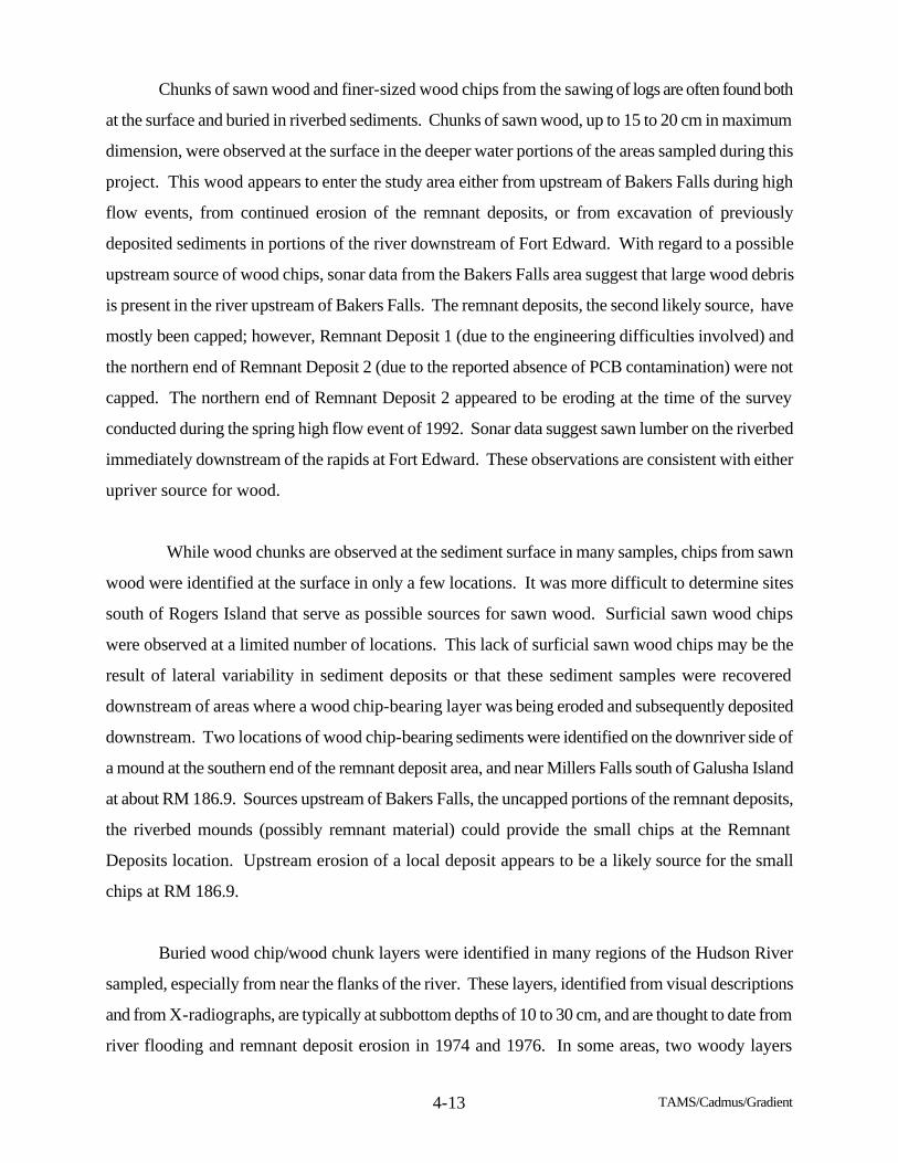
TAMS/Cadmus/Gradient 4-13
Chunks of sawn wood and finer-sized wood chips from the sawing of logs are often found both
at the surface and buried in riverbed sediments. Chunks of sawn wood, up to 15 to 20 cm in maximum
dimension, were observed at the surface in the deeper water portions of the areas sampled during this
project. This wood appears to enter the study area either from upstream of Bakers Falls during high
flow events, from continued erosion of the remnant deposits, or from excavation of previously
deposited sediments in portions of the river downstream of Fort Edward. With regard to a possible
upstream source of wood chips, sonar data from the Bakers Falls area suggest that large wood debris
is present in the river upstream of Bakers Falls. The remnant deposits, the second likely source, have
mostly been capped; however, Remnant Deposit 1 (due to the engineering difficulties involved) and
the northern end of Remnant Deposit 2 (due to the reported absence of PCB contamination) were not
capped. The northern end of Remnant Deposit 2 appeared to be eroding at the time of the survey
conducted during the spring high flow event of 1992. Sonar data suggest sawn lumber on the riverbed
immediately downstream of the rapids at Fort Edward. These observations are consistent with either
upriver source for wood.
While wood chunks are observed at the sediment surface in many samples, chips from sawn
wood were identified at the surface in only a few locations. It was more difficult to determine sites
south of Rogers Island that serve as possible sources for sawn wood. Surficial sawn wood chips
were observed at a limited number of locations. This lack of surficial sawn wood chips may be the
result of lateral variability in sediment deposits or that these sediment samples were recovered
downstream of areas where a wood chip-bearing layer was being eroded and subsequently deposited
downstream. Two locations of wood chip-bearing sediments were identified on the downriver side of
a mound at the southern end of the remnant deposit area, and near Millers Falls south of Galusha Island
at about RM 186.9. Sources upstream of Bakers Falls, the uncapped portions of the remnant deposits,
the riverbed mounds (possibly remnant material) could provide the small chips at the Remnant
Deposits location. Upstream erosion of a local deposit appears to be a likely source for the small
chips at RM 186.9.
Buried wood chip/wood chunk layers were identified in many regions of the Hudson River
sampled, especially from near the flanks of the river. These layers, identified from visual descriptions
and from X-radiographs, are typically at subbottom depths of 10 to 30 cm, and are thought to date from
river flooding and remnant deposit erosion in 1974 and 1976. In some areas, two woody layers
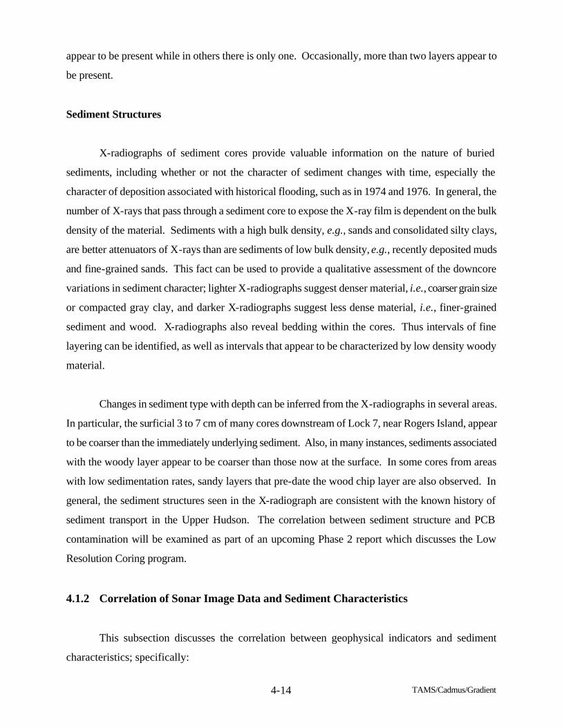
TAMS/Cadmus/Gradient 4-14
appear to be present while in others there is only one. Occasionally, more than two layers appear to
be present.
Sediment Structures
X-radiographs of sediment cores provide valuable information on the nature of buried
sediments, including whether or not the character of sediment changes with time, especially the
character of deposition associated with historical flooding, such as in 1974 and 1976. In general, the
number of X-rays that pass through a sediment core to expose the X-ray film is dependent on the bulk
density of the material. Sediments with a high bulk density, e.g., sands and consolidated silty clays,
are better attenuators of X-rays than are sediments of low bulk density, e.g., recently deposited muds
and fine-grained sands. This fact can be used to provide a qualitative assessment of the downcore
variations in sediment character; lighter X-radiographs suggest denser material, i.e., coarser grain size
or compacted gray clay, and darker X-radiographs suggest less dense material, i.e., finer-grained
sediment and wood. X-radiographs also reveal bedding within the cores. Thus intervals of fine
layering can be identified, as well as intervals that appear to be characterized by low density woody
material.
Changes in sediment type with depth can be inferred from the X-radiographs in several areas.
In particular, the surficial 3 to 7 cm of many cores downstream of Lock 7, near Rogers Island, appear
to be coarser than the immediately underlying sediment. Also, in many instances, sediments associated
with the woody layer appear to be coarser than those now at the surface. In some cores from areas
with low sedimentation rates, sandy layers that pre-date the wood chip layer are also observed. In
general, the sediment structures seen in the X-radiograph are consistent with the known history of
sediment transport in the Upper Hudson. The correlation between sediment structure and PCB
contamination will be examined as part of an upcoming Phase 2 report which discusses the Low
Resolution Coring program.
4.1.2 Correlation of Sonar Image Data and Sediment Characteristics
This subsection discusses the correlation between geophysical indicators and sediment
characteristics; specifically:
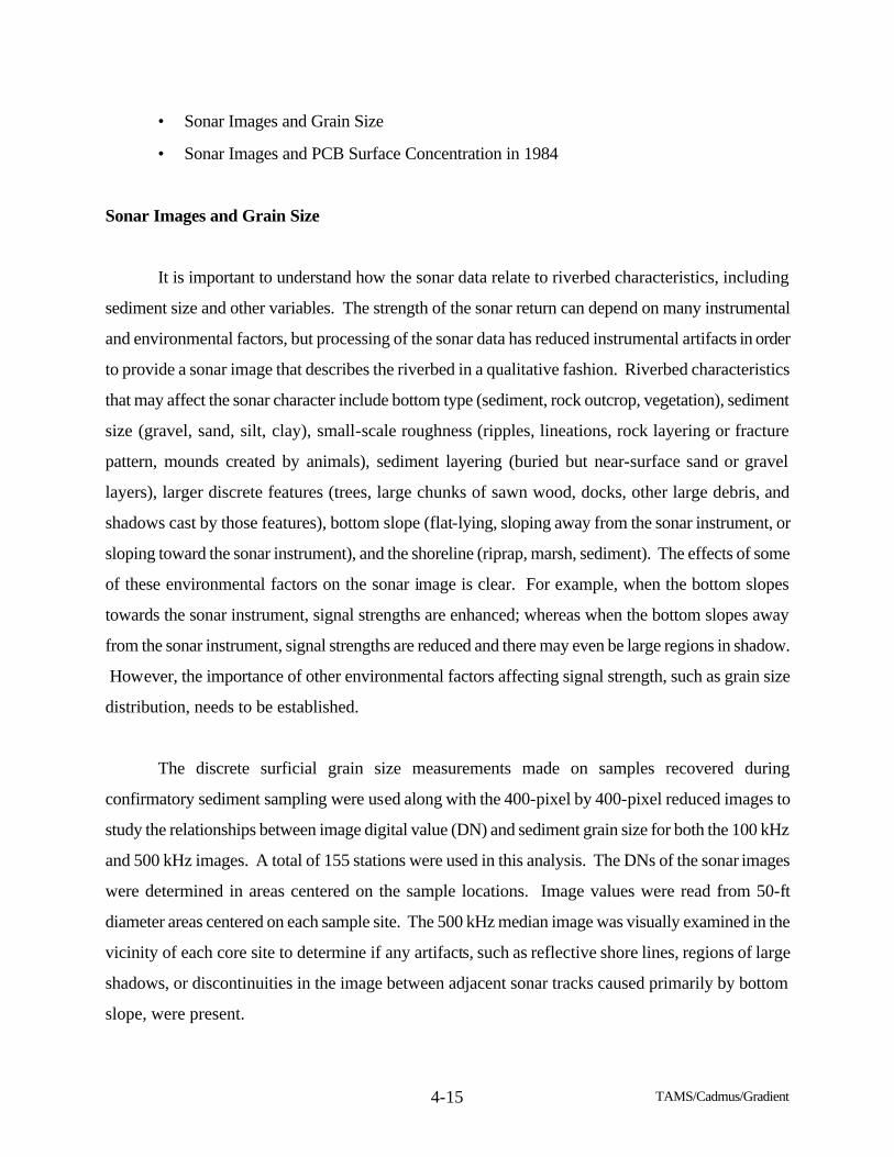
TAMS/Cadmus/Gradient 4-15
• Sonar Images and Grain Size
• Sonar Images and PCB Surface Concentration in 1984
Sonar Images and Grain Size
It is important to understand how the sonar data relate to riverbed characteristics, including
sediment size and other variables. The strength of the sonar return can depend on many instrumental
and environmental factors, but processing of the sonar data has reduced instrumental artifacts in order
to provide a sonar image that describes the riverbed in a qualitative fashion. Riverbed characteristics
that may affect the sonar character include bottom type (sediment, rock outcrop, vegetation), sediment
size (gravel, sand, silt, clay), small-scale roughness (ripples, lineations, rock layering or fracture
pattern, mounds created by animals), sediment layering (buried but near-surface sand or gravel
layers), larger discrete features (trees, large chunks of sawn wood, docks, other large debris, and
shadows cast by those features), bottom slope (flat-lying, sloping away from the sonar instrument, or
sloping toward the sonar instrument), and the shoreline (riprap, marsh, sediment). The effects of some
of these environmental factors on the sonar image is clear. For example, when the bottom slopes
towards the sonar instrument, signal strengths are enhanced; whereas when the bottom slopes away
from the sonar instrument, signal strengths are reduced and there may even be large regions in shadow.
However, the importance of other environmental factors affecting signal strength, such as grain size
distribution, needs to be established.
The discrete surficial grain size measurements made on samples recovered during
confirmatory sediment sampling were used along with the 400-pixel by 400-pixel reduced images to
study the relationships between image digital value (DN) and sediment grain size for both the 100 kHz
and 500 kHz images. A total of 155 stations were used in this analysis. The DNs of the sonar images
were determined in areas centered on the sample locations. Image values were read from 50-ft
diameter areas centered on each sample site. The 500 kHz median image was visually examined in the
vicinity of each core site to determine if any artifacts, such as reflective shore lines, regions of large
shadows, or discontinuities in the image between adjacent sonar tracks caused primarily by bottom
slope, were present.
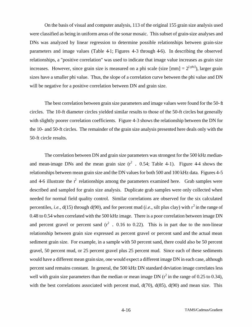
TAMS/Cadmus/Gradient 4-16
On the basis of visual and computer analysis, 113 of the original 155 grain size analysis used
were classified as being in uniform areas of the sonar mosaic. This subset of grain-size analyses and
DNs was analyzed by linear regression to determine possible relationships between grain-size
parameters and image values (Table 4-1; Figures 4-3 through 4-6). In describing the observed
relationships, a "positive correlation" was used to indicate that image value increases as grain size
increases. However, since grain size is measured on a phi scale (size [mm] = 2[-phi]), larger grain
sizes have a smaller phi value. Thus, the slope of a correlation curve between the phi value and DN
will be negative for a positive correlation between DN and grain size.
The best correlation between grain size parameters and image values were found for the 50- ft
circles. The 10-ft diameter circles yielded similar results to those of the 50-ft circles but generally
with slightly poorer correlation coefficients. Figure 4-3 shows the relationship between the DN for
the 10- and 50-ft circles. The remainder of the grain size analysis presented here deals only with the
50-ft circle results.
The correlation between DN and grain size parameters was strongest for the 500 kHz median-
and mean-image DNs and the mean grain size (r2 . 0.54; Table 4-1). Figure 4-4 shows the
relationships between mean grain size and the DN values for both 500 and 100 kHz data. Figures 4-5
and 4-6 illustrate the r2 relationships among the parameters examined here. Grab samples were
described and sampled for grain size analysis. Duplicate grab samples were only collected when
needed for normal field quality control. Similar correlations are observed for the six calculated
percentiles, i.e., d(15) through d(90), and for percent mud (i.e., silt plus clay) with r2 in the range of
0.48 to 0.54 when correlated with the 500 kHz image. There is a poor correlation between image DN
and percent gravel or percent sand (r2 . 0.16 to 0.22). This is in part due to the non-linear
relationship between grain size expressed as percent gravel or percent sand and the actual mean
sediment grain size. For example, in a sample with 50 percent sand, there could also be 50 percent
gravel, 50 percent mud, or 25 percent gravel plus 25 percent mud. Since each of these sediments
would have a different mean grain size, one would expect a different image DN in each case, although
percent sand remains constant. In general, the 500 kHz DN standard deviation image correlates less
well with grain size parameters than the median or mean image DN (r2 in the range of 0.25 to 0.34),
with the best correlations associated with percent mud, d(70), d(85), d(90) and mean size. This
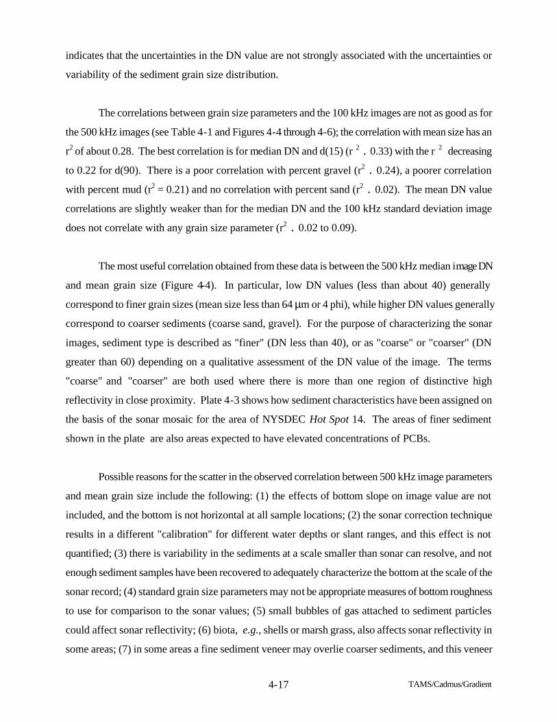
TAMS/Cadmus/Gradient 4-17
indicates that the uncertainties in the DN value are not strongly associated with the uncertainties or
variability of the sediment grain size distribution.
The correlations between grain size parameters and the 100 kHz images are not as good as for
the 500 kHz images (see Table 4-1 and Figures 4-4 through 4-6); the correlation with mean size has an
r2 of about 0.28. The best correlation is for median DN and d(15) (r 2 . 0.33) with the r 2 decreasing
to 0.22 for d(90). There is a poor correlation with percent gravel (r2 . 0.24), a poorer correlation
with percent mud (r2 = 0.21) and no correlation with percent sand (r2 . 0.02). The mean DN value
correlations are slightly weaker than for the median DN and the 100 kHz standard deviation image
does not correlate with any grain size parameter (r2 . 0.02 to 0.09).
The most useful correlation obtained from these data is between the 500 kHz median image DN
and mean grain size (Figure 4-4). In particular, low DN values (less than about 40) generally
correspond to finer grain sizes (mean size less than 64 µm or 4 phi), while higher DN values generally
correspond to coarser sediments (coarse sand, gravel). For the purpose of characterizing the sonar
images, sediment type is described as "finer" (DN less than 40), or as "coarse" or "coarser" (DN
greater than 60) depending on a qualitative assessment of the DN value of the image. The terms
"coarse" and "coarser" are both used where there is more than one region of distinctive high
reflectivity in close proximity. Plate 4-3 shows how sediment characteristics have been assigned on
the basis of the sonar mosaic for the area of NYSDEC Hot Spot 14. The areas of finer sediment
shown in the plate are also areas expected to have elevated concentrations of PCBs.
Possible reasons for the scatter in the observed correlation between 500 kHz image parameters
and mean grain size include the following: (1) the effects of bottom slope on image value are not
included, and the bottom is not horizontal at all sample locations; (2) the sonar correction technique
results in a different "calibration" for different water depths or slant ranges, and this effect is not
quantified; (3) there is variability in the sediments at a scale smaller than sonar can resolve, and not
enough sediment samples have been recovered to adequately characterize the bottom at the scale of the
sonar record; (4) standard grain size parameters may not be appropriate measures of bottom roughness
to use for comparison to the sonar values; (5) small bubbles of gas attached to sediment particles
could affect sonar reflectivity; (6) biota, e.g., shells or marsh grass, also affects sonar reflectivity in
some areas; (7) in some areas a fine sediment veneer may overlie coarser sediments, and this veneer
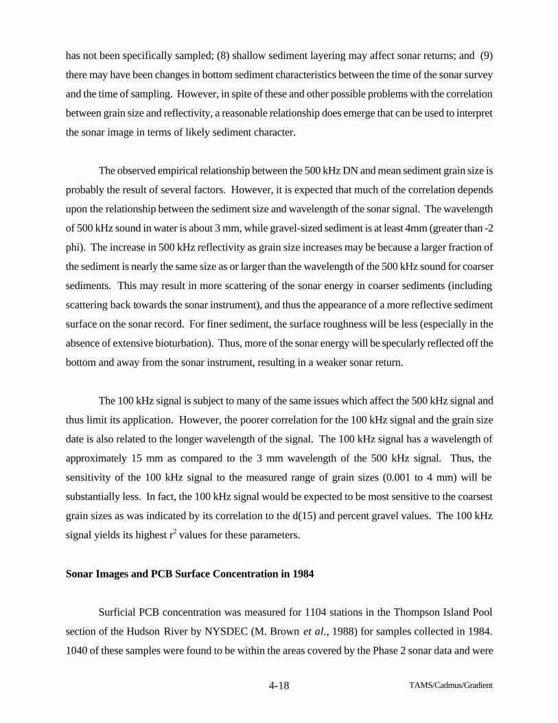
TAMS/Cadmus/Gradient 4-18
has not been specifically sampled; (8) shallow sediment layering may affect sonar returns; and (9)
there may have been changes in bottom sediment characteristics between the time of the sonar survey
and the time of sampling. However, in spite of these and other possible problems with the correlation
between grain size and reflectivity, a reasonable relationship does emerge that can be used to interpret
the sonar image in terms of likely sediment character.
The observed empirical relationship between the 500 kHz DN and mean sediment grain size is
probably the result of several factors. However, it is expected that much of the correlation depends
upon the relationship between the sediment size and wavelength of the sonar signal. The wavelength
of 500 kHz sound in water is about 3 mm, while gravel-sized sediment is at least 4mm (greater than -2
phi). The increase in 500 kHz reflectivity as grain size increases may be because a larger fraction of
the sediment is nearly the same size as or larger than the wavelength of the 500 kHz sound for coarser
sediments. This may result in more scattering of the sonar energy in coarser sediments (including
scattering back towards the sonar instrument), and thus the appearance of a more reflective sediment
surface on the sonar record. For finer sediment, the surface roughness will be less (especially in the
absence of extensive bioturbation). Thus, more of the sonar energy will be specularly reflected off the
bottom and away from the sonar instrument, resulting in a weaker sonar return.
The 100 kHz signal is subject to many of the same issues which affect the 500 kHz signal and
thus limit its application. However, the poorer correlation for the 100 kHz signal and the grain size
date is also related to the longer wavelength of the signal. The 100 kHz signal has a wavelength of
approximately 15 mm as compared to the 3 mm wavelength of the 500 kHz signal. Thus, the
sensitivity of the 100 kHz signal to the measured range of grain sizes (0.001 to 4 mm) will be
substantially less. In fact, the 100 kHz signal would be expected to be most sensitive to the coarsest
grain sizes as was indicated by its correlation to the d(15) and percent gravel values. The 100 kHz
signal yields its highest r2 values for these parameters.
Sonar Images and PCB Surface Concentration in 1984
Surficial PCB concentration was measured for 1104 stations in the Thompson Island Pool
section of the Hudson River by NYSDEC (M. Brown et al., 1988) for samples collected in 1984.
1040 of these samples were found to be within the areas covered by the Phase 2 sonar data and were
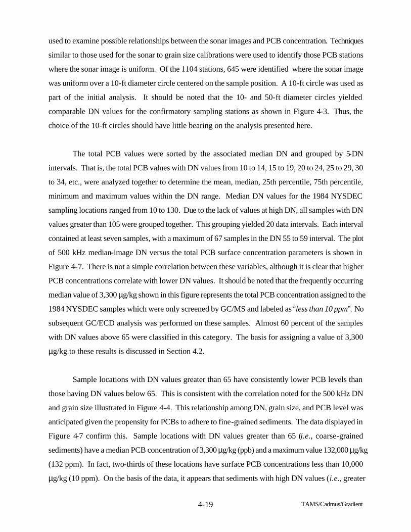
TAMS/Cadmus/Gradient 4-19
used to examine possible relationships between the sonar images and PCB concentration. Techniques
similar to those used for the sonar to grain size calibrations were used to identify those PCB stations
where the sonar image is uniform. Of the 1104 stations, 645 were identified where the sonar image
was uniform over a 10-ft diameter circle centered on the sample position. A 10-ft circle was used as
part of the initial analysis. It should be noted that the 10- and 50-ft diameter circles yielded
comparable DN values for the confirmatory sampling stations as shown in Figure 4-3. Thus, the
choice of the 10-ft circles should have little bearing on the analysis presented here.
The total PCB values were sorted by the associated median DN and grouped by 5-DN
intervals. That is, the total PCB values with DN values from 10 to 14, 15 to 19, 20 to 24, 25 to 29, 30
to 34, etc., were analyzed together to determine the mean, median, 25th percentile, 75th percentile,
minimum and maximum values within the DN range. Median DN values for the 1984 NYSDEC
sampling locations ranged from 10 to 130. Due to the lack of values at high DN, all samples with DN
values greater than 105 were grouped together. This grouping yielded 20 data intervals. Each interval
contained at least seven samples, with a maximum of 67 samples in the DN 55 to 59 interval. The plot
of 500 kHz median-image DN versus the total PCB surface concentration parameters is shown in
Figure 4-7. There is not a simple correlation between these variables, although it is clear that higher
PCB concentrations correlate with lower DN values. It should be noted that the frequently occurring
median value of 3,300 µg/kg shown in this figure represents the total PCB concentration assigned to the
1984 NYSDEC samples which were only screened by GC/MS and labeled as Aless than 10 ppm@. No
subsequent GC/ECD analysis was performed on these samples. Almost 60 percent of the samples
with DN values above 65 were classified in this category. The basis for assigning a value of 3,300
µg/kg to these results is discussed in Section 4.2.
Sample locations with DN values greater than 65 have consistently lower PCB levels than
those having DN values below 65. This is consistent with the correlation noted for the 500 kHz DN
and grain size illustrated in Figure 4-4. This relationship among DN, grain size, and PCB level was
anticipated given the propensity for PCBs to adhere to fine-grained sediments. The data displayed in
Figure 4-7 confirm this. Sample locations with DN values greater than 65 (i.e., coarse-grained
sediments) have a median PCB concentration of 3,300 µg/kg (ppb) and a maximum value 132,000 µg/kg
(132 ppm). In fact, two-thirds of these locations have surface PCB concentrations less than 10,000
µg/kg (10 ppm). On the basis of the data, it appears that sediments with high DN values (i.e., greater
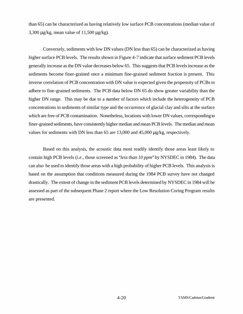
TAMS/Cadmus/Gradient 4-20
than 65) can be characterized as having relatively low surface PCB concentrations (median value of
3,300 µg/kg, mean value of 11,500 µg/kg).
Conversely, sediments with low DN values (DN less than 65) can be characterized as having
higher surface PCB levels. The results shown in Figure 4-7 indicate that surface sediment PCB levels
generally increase as the DN value decreases below 65. This suggests that PCB levels increase as the
sediments become finer-grained once a minimum fine-grained sediment fraction is present. This
inverse correlation of PCB concentration with DN value is expected given the propensity of PCBs to
adhere to fine-grained sediments. The PCB data below DN 65 do show greater variability than the
higher DN range. This may be due to a number of factors which include the heterogeneity of PCB
concentrations in sediments of similar type and the occurrence of glacial clay and silts at the surface
which are free of PCB contamination. Nonetheless, locations with lower DN values, corresponding to
finer-grained sediments, have consistently higher median and mean PCB levels. The median and mean
values for sediments with DN less than 65 are 13,000 and 45,000 µg/kg, respectively.
Based on this analysis, the acoustic data most readily identify those areas least likely to
contain high PCB levels (i.e., those screened as Aless than 10 ppm@ by NYSDEC in 1984). The data
can also be used to identify those areas with a high probability of higher PCB levels. This analysis is
based on the assumption that conditions measured during the 1984 PCB survey have not changed
drastically. The extent of change in the sediment PCB levels determined by NYSDEC in 1984 will be
assessed as part of the subsequent Phase 2 report where the Low Resolution Coring Program results
are presented.
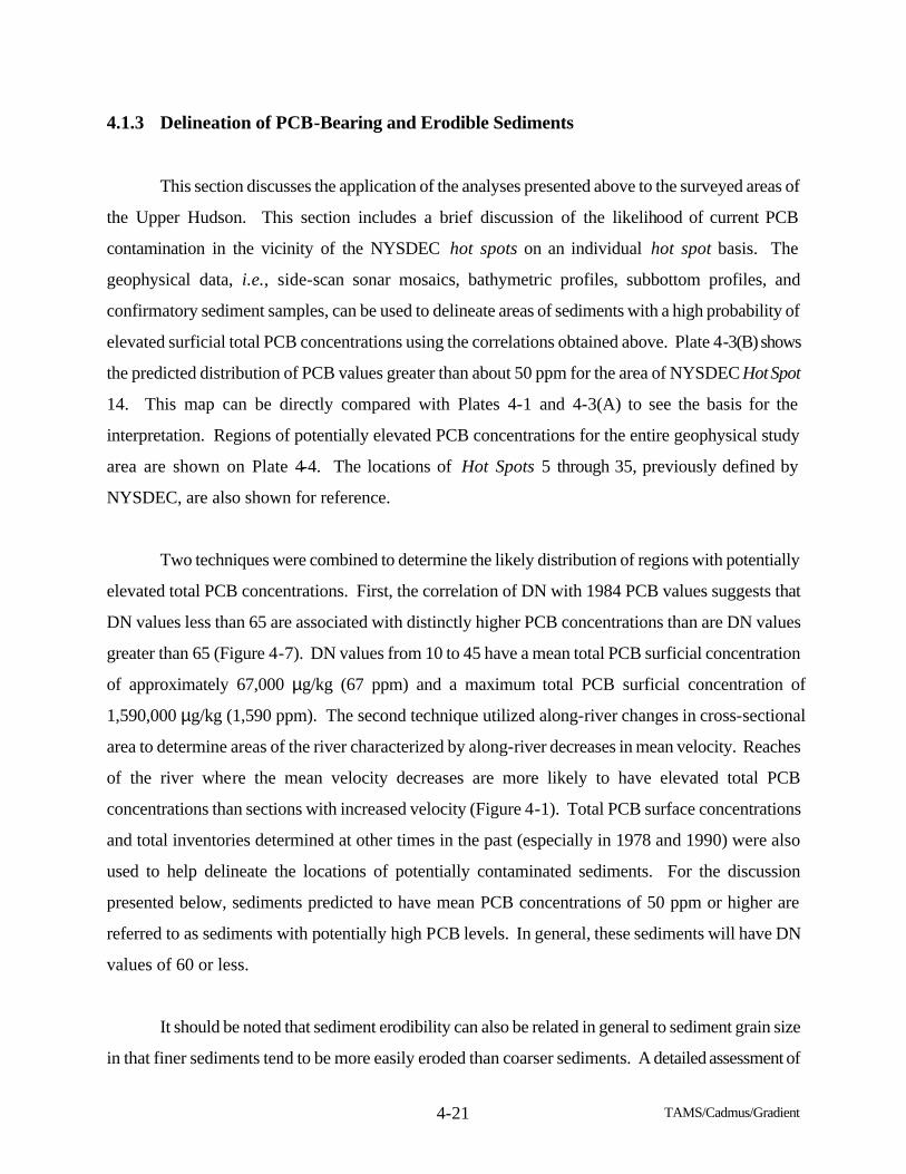
TAMS/Cadmus/Gradient 4-21
4.1.3 Delineation of PCB-Bearing and Erodible Sediments
This section discusses the application of the analyses presented above to the surveyed areas of
the Upper Hudson. This section includes a brief discussion of the likelihood of current PCB
contamination in the vicinity of the NYSDEC hot spots on an individual hot spot basis. The
geophysical data, i.e., side-scan sonar mosaics, bathymetric profiles, subbottom profiles, and
confirmatory sediment samples, can be used to delineate areas of sediments with a high probability of
elevated surficial total PCB concentrations using the correlations obtained above. Plate 4-3(B) shows
the predicted distribution of PCB values greater than about 50 ppm for the area of NYSDEC Hot Spot
14. This map can be directly compared with Plates 4-1 and 4-3(A) to see the basis for the
interpretation. Regions of potentially elevated PCB concentrations for the entire geophysical study
area are shown on Plate 4-4. The locations of Hot Spots 5 through 35, previously defined by
NYSDEC, are also shown for reference.
Two techniques were combined to determine the likely distribution of regions with potentially
elevated total PCB concentrations. First, the correlation of DN with 1984 PCB values suggests that
DN values less than 65 are associated with distinctly higher PCB concentrations than are DN values
greater than 65 (Figure 4-7). DN values from 10 to 45 have a mean total PCB surficial concentration
of approximately 67,000 µg/kg (67 ppm) and a maximum total PCB surficial concentration of
1,590,000 µg/kg (1,590 ppm). The second technique utilized along-river changes in cross-sectional
area to determine areas of the river characterized by along-river decreases in mean velocity. Reaches
of the river where the mean velocity decreases are more likely to have elevated total PCB
concentrations than sections with increased velocity (Figure 4-1). Total PCB surface concentrations
and total inventories determined at other times in the past (especially in 1978 and 1990) were also
used to help delineate the locations of potentially contaminated sediments. For the discussion
presented below, sediments predicted to have mean PCB concentrations of 50 ppm or higher are
referred to as sediments with potentially high PCB levels. In general, these sediments will have DN
values of 60 or less.
It should be noted that sediment erodibility can also be related in general to sediment grain size
in that finer sediments tend to be more easily eroded than coarser sediments. A detailed assessment of
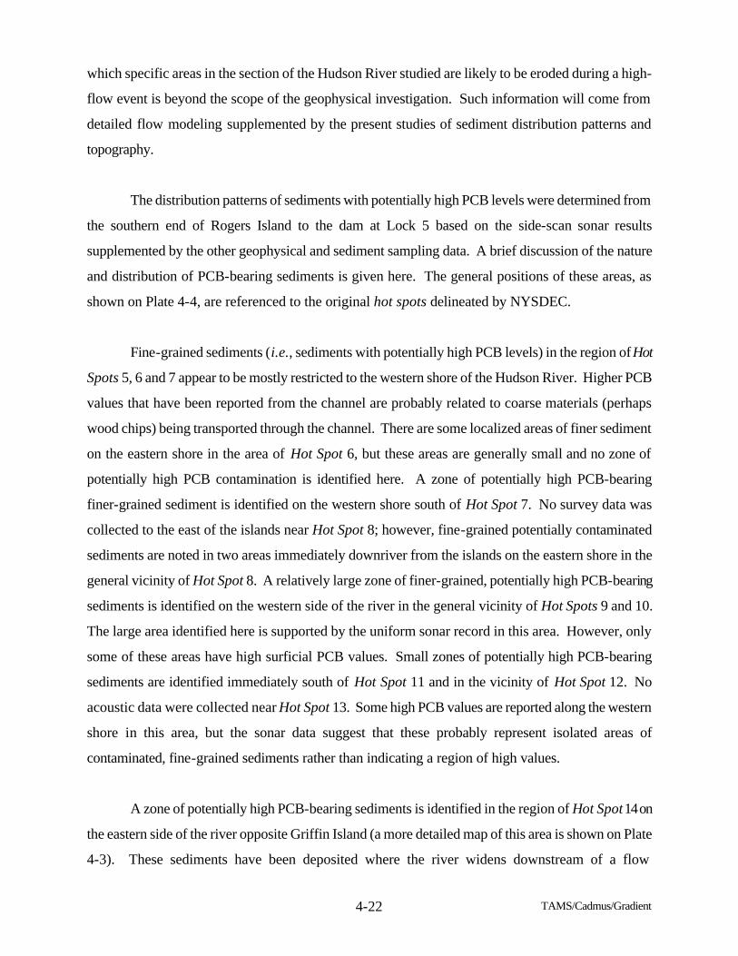
TAMS/Cadmus/Gradient 4-22
which specific areas in the section of the Hudson River studied are likely to be eroded during a high-
flow event is beyond the scope of the geophysical investigation. Such information will come from
detailed flow modeling supplemented by the present studies of sediment distribution patterns and
topography.
The distribution patterns of sediments with potentially high PCB levels were determined from
the southern end of Rogers Island to the dam at Lock 5 based on the side-scan sonar results
supplemented by the other geophysical and sediment sampling data. A brief discussion of the nature
and distribution of PCB-bearing sediments is given here. The general positions of these areas, as
shown on Plate 4-4, are referenced to the original hot spots delineated by NYSDEC.
Fine-grained sediments (i.e., sediments with potentially high PCB levels) in the region of Hot
Spots 5, 6 and 7 appear to be mostly restricted to the western shore of the Hudson River. Higher PCB
values that have been reported from the channel are probably related to coarse materials (perhaps
wood chips) being transported through the channel. There are some localized areas of finer sediment
on the eastern shore in the area of Hot Spot 6, but these areas are generally small and no zone of
potentially high PCB contamination is identified here. A zone of potentially high PCB-bearing
finer-grained sediment is identified on the western shore south of Hot Spot 7. No survey data was
collected to the east of the islands near Hot Spot 8; however, fine-grained potentially contaminated
sediments are noted in two areas immediately downriver from the islands on the eastern shore in the
general vicinity of Hot Spot 8. A relatively large zone of finer-grained, potentially high PCB-bearing
sediments is identified on the western side of the river in the general vicinity of Hot Spots 9 and 10.
The large area identified here is supported by the uniform sonar record in this area. However, only
some of these areas have high surficial PCB values. Small zones of potentially high PCB-bearing
sediments are identified immediately south of Hot Spot 11 and in the vicinity of Hot Spot 12. No
acoustic data were collected near Hot Spot 13. Some high PCB values are reported along the western
shore in this area, but the sonar data suggest that these probably represent isolated areas of
contaminated, fine-grained sediments rather than indicating a region of high values.
A zone of potentially high PCB-bearing sediments is identified in the region of Hot Spot 14 on
the eastern side of the river opposite Griffin Island (a more detailed map of this area is shown on Plate
4-3). These sediments have been deposited where the river widens downstream of a flow
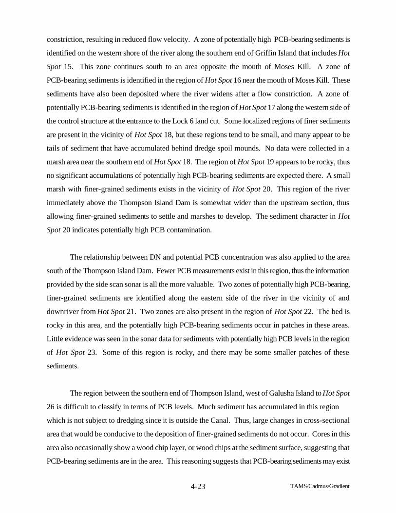
TAMS/Cadmus/Gradient 4-23
constriction, resulting in reduced flow velocity. A zone of potentially high PCB-bearing sediments is
identified on the western shore of the river along the southern end of Griffin Island that includes Hot
Spot 15. This zone continues south to an area opposite the mouth of Moses Kill. A zone of
PCB-bearing sediments is identified in the region of Hot Spot 16 near the mouth of Moses Kill. These
sediments have also been deposited where the river widens after a flow constriction. A zone of
potentially PCB-bearing sediments is identified in the region of Hot Spot 17 along the western side of
the control structure at the entrance to the Lock 6 land cut. Some localized regions of finer sediments
are present in the vicinity of Hot Spot 18, but these regions tend to be small, and many appear to be
tails of sediment that have accumulated behind dredge spoil mounds. No data were collected in a
marsh area near the southern end of Hot Spot 18. The region of Hot Spot 19 appears to be rocky, thus
no significant accumulations of potentially high PCB-bearing sediments are expected there. A small
marsh with finer-grained sediments exists in the vicinity of Hot Spot 20. This region of the river
immediately above the Thompson Island Dam is somewhat wider than the upstream section, thus
allowing finer-grained sediments to settle and marshes to develop. The sediment character in Hot
Spot 20 indicates potentially high PCB contamination.
The relationship between DN and potential PCB concentration was also applied to the area
south of the Thompson Island Dam. Fewer PCB measurements exist in this region, thus the information
provided by the side scan sonar is all the more valuable. Two zones of potentially high PCB-bearing,
finer-grained sediments are identified along the eastern side of the river in the vicinity of and
downriver from Hot Spot 21. Two zones are also present in the region of Hot Spot 22. The bed is
rocky in this area, and the potentially high PCB-bearing sediments occur in patches in these areas.
Little evidence was seen in the sonar data for sediments with potentially high PCB levels in the region
of Hot Spot 23. Some of this region is rocky, and there may be some smaller patches of these
sediments.
The region between the southern end of Thompson Island, west of Galusha Island to Hot Spot
26 is difficult to classify in terms of PCB levels. Much sediment has accumulated in this region
which is not subject to dredging since it is outside the Canal. Thus, large changes in cross-sectional
area that would be conducive to the deposition of finer-grained sediments do not occur. Cores in this
area also occasionally show a wood chip layer, or wood chips at the sediment surface, suggesting that
PCB-bearing sediments are in the area. This reasoning suggests that PCB-bearing sediments may exist
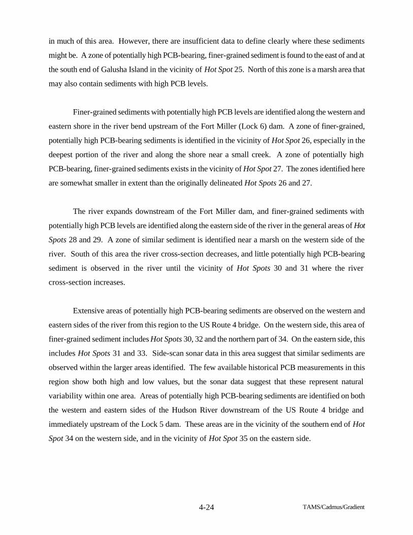
TAMS/Cadmus/Gradient 4-24
in much of this area. However, there are insufficient data to define clearly where these sediments
might be. A zone of potentially high PCB-bearing, finer-grained sediment is found to the east of and at
the south end of Galusha Island in the vicinity of Hot Spot 25. North of this zone is a marsh area that
may also contain sediments with high PCB levels.
Finer-grained sediments with potentially high PCB levels are identified along the western and
eastern shore in the river bend upstream of the Fort Miller (Lock 6) dam. A zone of finer-grained,
potentially high PCB-bearing sediments is identified in the vicinity of Hot Spot 26, especially in the
deepest portion of the river and along the shore near a small creek. A zone of potentially high
PCB-bearing, finer-grained sediments exists in the vicinity of Hot Spot 27. The zones identified here
are somewhat smaller in extent than the originally delineated Hot Spots 26 and 27.
The river expands downstream of the Fort Miller dam, and finer-grained sediments with
potentially high PCB levels are identified along the eastern side of the river in the general areas of Hot
Spots 28 and 29. A zone of similar sediment is identified near a marsh on the western side of the
river. South of this area the river cross-section decreases, and little potentially high PCB-bearing
sediment is observed in the river until the vicinity of Hot Spots 30 and 31 where the river
cross-section increases.
Extensive areas of potentially high PCB-bearing sediments are observed on the western and
eastern sides of the river from this region to the US Route 4 bridge. On the western side, this area of
finer-grained sediment includes Hot Spots 30, 32 and the northern part of 34. On the eastern side, this
includes Hot Spots 31 and 33. Side-scan sonar data in this area suggest that similar sediments are
observed within the larger areas identified. The few available historical PCB measurements in this
region show both high and low values, but the sonar data suggest that these represent natural
variability within one area. Areas of potentially high PCB-bearing sediments are identified on both
the western and eastern sides of the Hudson River downstream of the US Route 4 bridge and
immediately upstream of the Lock 5 dam. These areas are in the vicinity of the southern end of Hot
Spot 34 on the western side, and in the vicinity of Hot Spot 35 on the eastern side.
4-25
4.2 Geostatistical Analysis of PCB Mass in the Thompson Island Pool, 1984
A geostatistical analysis of the NYSDEC 1984 survey of PCB contamination in the Thompson
Island Pool was completed to assess the accuracy of the original, more subjective assessment
completed by M. Brown et al., 1988. As noted in the Phase 1 Report (TAMS/Gradient, 1991), the
1984 sediment survey revealed a high degree of heterogeneity in the distribution of PCBs in Thompson
Island Pool sediments. Indeed, it was not unusual for samples taken only a few meters apart
horizontally to exhibit order-of-magnitude differences in PCB concentrations, and results along some
transects across the river ranged from nondetectable to greater than 1000 ppm. On the other hand, it
was also clear that there was spatial correlation in PCB concentrations, reflected in the delineation of
a number of PCB hot spots.
In an earlier analysis of the 1984 results, M. Brown et al. (1988) estimated the total PCB mass
in the Thompson Island Pool sediments at 23,200 kg (23.2 metric tons). However, questions have
been raised regarding the methods used to obtain this estimate, suggesting that a reanalysis of the data
was appropriate. In the procedure adopted by M. Brown et al., the Thompson Island Pool was
subdivided into 138 polygonal areas wherein the means of unit-area PCB mass were calculated over
each area, and the total PCB mass was summed. This approach admittedly neglected the fact that the
sampling was not random, but instead was intentionally focused on (1) previously identified hot spots
and (2) soft organic, coreable sediments, which are also suspected to be associated with higher PCB
levels due to partitioning to organic carbon. Both sample biases might have led to an overestimation
of PCB mass. Errors in measurement of sediment density and porosity may also have led to
overestimation. In addition, M. Brown et al. did not take into account the effects of spatial correlation
on the estimates. The TAMS/Gradient team therefore reanalyzed the data using more sophisticated
mathematical tools and compared the result to the original estimate.
The present analysis uses several methods to generate mass estimates of the same order of
magnitude, but 16 percent to 38 percent smaller than the mass reported by M. Brown et al. These
methods also provide a continuous spatial description of the data, which is more useful for
interpolation and for comparison of 1984 results to data for sediment samples obtained in the
Reassessment. Finally, maps and estimates of surface concentrations in 1984 were developed for use
in consideration of biological pathways from the sediments into the aquatic food chain.
TAMS/Cadmus/Gradient 4-26
4.2.1 Data Preparation for PCB Mass Estimation
PCB data are reported by M. Brown et al. on a concentration basis as ppm, or µg/g sediment
(dry-weight). For mass estimation, these concentrations must be converted to mass units by
multiplying by the density. Summing mass in the vertical dimension yields mass per unit surface area.
Mass units are additive (unlike concentration) and appropriate for spatial analyses, such as kriging.
Estimates of the total PCB mass present in 1984 are sensitive to the methods and assumptions
used to convert concentration data to mass units, as well as to any inaccuracies in the methods
employed by NYSDEC to estimate concentration and density. The assumptions used by M. Brown et
al. (1988) were reviewed and critiqued. The assumptions used by the TAMS/Gradient team in
preparing the data are largely similar to those of M. Brown et al., but differ in certain important
aspects. In addition, the accuracy of some of the analytical methods employed in 1984 is questionable.
Data quality and data preparation for the current estimates are thus documented in detail.
Analytical Results for Total PCBs
The estimates of total PCB mass depend directly on the total PCB concentrations reported by
NYSDEC. This total is based on the sum of Aroclor quantitations, which may not accurately reflect
the actual sum of PCB congeners present, particularly when environmental degradation has altered the
congener composition of the original Aroclors.
To quantitate Aroclors, NYSDEC used packed-column gas chromatography with electron
capture detection (M. Brown and Werner, 1984). NYSDEC's contractor, Versar, calculated
concentrations of Aroclor 1242, Aroclor 1254 and Aroclor 1260 using the method of Webb and
McCall (1973). However, M. Brown et al. (1988) noted "Upon examination of sample
chromatograms, it became apparent that . . . sample peaks were assigned subjectively rather than
strictly using relative retention times developed from interpretation of Aroclor standards. . .
[D]ifferences in columns and GC operating conditions between Versar and Webb and McCall (1973)
resulted in a lack of strict correspondence between relative retention times. This problem in addition
TAMS/Cadmus/Gradient 4-27
to presence of peaks apparently missed by the peak integrator resulted in a high frequency of certain
peaks not being quantitated."
Most of the missed peaks were in the Aroclor 1242 range. NYSDEC therefore recalculated
the Aroclor 1242 concentrations after development of three total Aroclor 1242 response factors
corresponding to three separate packed-column peaks. These response factors were applied to the
three peaks for each sample to generate three estimates of the Aroclor 1242 concentration. The
average of the three Aroclor 1242 concentrations was reported as the Aroclor 1242 concentration for
the sample. The three peaks used were the same ones used by O'Brien and Gere for Aroclor 1016 in
the 1978 analysis. In order to estimate the total PCB concentration for the sample, A[t]he sum of the
recalculated Aroclor 1242 concentration and the PCB concentrations reported as Aroclor 1254 and
Aroclor 1260 by Versar was employed as the total PCB concentration in this analysis" (M. Brown et
al., 1988). In sum, the total PCB concentrations reported by NYSDEC are indirect approximations.
However, these approximations constitute the best available data for estimation of PCB mass
historically present in the sediments.
Use of Screening Data
The analytical protocol (M. Brown and Werner, 1984) called for most, but not all, samples to
be screened by gas chromatography/mass spectrometry (GC/MS) prior to deciding whether to
undertake a more expensive gas chromatography analysis with an electron capture detector (GC/ECD).
Screening was accomplished with a mobile mass spectrometer system (Trace Atmospheric Gas
Analysis 3000 - TAGA), which measured the concentration ratio of PCBs in methylene chloride
extracts of sediment samples (M. Brown and Werner, 1984). The accuracy of the screening method
was relatively low, and results were reported as a classification into one of four ranges: less than
10 ppm (COLD); 10 to 50 ppm; 50 to 100 ppm; and greater than 100 ppm (HOT). Most samples
falling within the highest three screening categories were sent for GC/ECD analyses; however, only a
small proportion of samples from the less than 10 ppm category was analyzed by GC/ECD. In cores,
nearly all sections were screened, but typically only a few sections were analyzed by GC/ECD. It is
necessary to include the screening data in the calculations to properly evaluate the total PCB mass
within a core. The GC/MS data are, however, clearly less reliable than the GC/ECD data. GC/ECD
TAMS/Cadmus/Gradient 4-28
results were therefore regarded as strictly preferable, when both were available; GC/MS estimates
were substituted only when GC/ECD data were not available.
GC/MS screening ranges had to first be converted to approximate numerical values for use in
subsequent calculations. Because the distribution of the data was approximately log-normal, and the
kriging analysis was to be performed in log space, each screening range was represented by its
observed median, which is a robust estimator of the geometric mean. Basic data for comparisons of
497 split samples analyzed by both methods are shown in Table 4-2. This determination is most
critical for the less than 10 ppm screening data where only 6 percent of samples were subsequently
confirmed by GC/ECD; 75 percent of samples screened greater than this category were analyzed by
GC/ECD.
Present assumptions differ from those of M. Brown et al., who represented each GC/MS range
by the GC/ECD mean estimated from split samples. Notably, the estimated mean for the less than
10 ppm class was 15.0 mg/kg, which is outside the class boundary, as shown in Table 4-2. Similarly,
the value of 134.6 mg/kg used by M. Brown et al., for the 50-100 ppm category lies outside the class
boundary. In both instances, the standard deviation is large relative to the mean and the sample size is
small, therefore the mean may be distorted by a few large values. Because the data are apparently log-
normal, the median values are more appropriately representative of the central tendency of each range
and thus better point estimates for analysis of spatial correlation. The assumption that the median
values for these categories (3.3 mg/kg and 18.2 mg/kg, respectively) are more representative than the
(higher) mean values for these categories used by Brown will of course result in lower mass estimates
relative to Brown.
TAMS/Cadmus/Gradient 4-29
Vertical Summation of PCB Mass
Mass per unit surface area is determined by vertical summation of total PCB mass, which
requires defining the bottom depth of contamination. In cores, most sections that screened in the less
than 10 ppm range were not sent for GC/ECD analysis, and deeper sections often consist of a series of
less than 10 ppm screening results. The current analysis has adopted a protocol similar to that
employed by M. Brown et al. in which most less than 10 ppm screening sections are interpreted to
have the point estimate concentration, i.e., the median for the range as given in Table 4-2. Assigning
this finite concentration to an infinite depth, however, is unreasonable. Therefore, the second
consecutive and any succeeding deeper less than 10 ppm sections in a core for which there is no
evidence of PCB contamination at deeper levels are assigned a concentration of zero. Sections which
screened less than 10 ppm and are located below GC/ECD nondetects were also assigned zero values
(which apparently differs from the assumptions of M. Brown et al.).
The vertical summation assumed that PCB contamination was not present below the depth of
sampling. Mean core length for this survey was 31.1 inches, with cores advanced up to a maximum of
60 inches, depending on sediment characteristics. 121 out of 128 core sections collected from 30
inches in depth or greater screened as less than 10 ppm, so the assumption of no PCBs below the
bottom of a given core is unlikely to cause much error in the mass calculation. Estimating the depth of
contamination is more difficult for grab samples, for which a measured depth is not provided. Depth
of grab sampling was estimated to be 12 inches (31 cm) in gravel sediments, and 17 inches (43 cm) in
fine-grained sand and other sediments, following M. Brown et al. Grab samples were taken primarily
where the corer could not penetrate, particularly in gravels, where significant depth of accumulation of
contaminated sediments is unlikely.
Specific Weight of Sediment
Specific weight, or density, is required to translate from sediment concentration (reported on a
mass:mass dry-weight basis) to unit area mass (which requires a mass:volume basis). Multiplying by
specific weight (i.e., sediment dry mass per unit wet volume) converts concentration to mass. Errors
in specific weight measurement translate directly to errors in mass estimates.
The file provided by NYSDEC reports specific weight and percent dry solids (as weight
TAMS/Cadmus/Gradient 4-30
percent). This is not, however, what was measured. Referring to M. Brown et al. (1988, pp. 8 and
9):
Percent dry solids was determined by weight loss of a sediment aliquot dried at 100oC on a drying dish. To assess specific weight, sediment was carefully transferred to a 20 mL beaker. Sediment in the beaker was occasionally gently tamped to remove noticeable air pockets. Specific weight was estimated as the product of wet weight per unit volume of the 20 mL beaker and the percent dry solids.
Thus, NYSDEC measured (but did not report) wet density (weight per unit volume) and reported (but
did not directly measure) specific weight.
There are several problems with the analytical procedure used to determine specific weight.
Determination of wet weight per unit volume was done on a disturbed sample, and is unlikely to
reflect in situ conditions. Weight loss estimation was made at 100oC, rather than the usual 105oC,
and drying time is not documented. This procedure can result in a substantial overestimation of
percent solids, and thus of specific weight, especially for finer-grained sediments.
A calculation of the porosity of samples, which is implied by reported specific weight and
percent dry solids data, revealed a number of samples with physically inconsistent results of estimated
porosity greater than 100 percent. In addition, a large proportion of the samples have estimated
porosities which appear to be biased low due to the measurement technique used for specific weight.
The average specific weight across all samples analyzed by NYSDEC is 1.1 g/cm3. Conversely, the
Phase 2 high-resolution sediment coring results yielded an average specific weight for sediments in
the Upper Hudson of 0.77 g/cm3. Further, the over-estimation of specific weight by NYSDEC is
apparently greater for fine-grained sediments. If specific weight is, on average, over-estimated, the
PCB mass obtained from NYSDEC data is also over-estimated. However, the large degree of error
evident in porosity estimates makes a simple correction impossible.
Specific weight estimates were provided for most core samples. Specific weight for many of
the grab samples, however, was not reported, because the analytical method was not suitable for
gravel. M. Brown et al. noted this problem and analyzed 44 gravel samples by another method. This
method yielded a mean specific weight of 1.3 g/cm3, which was used for all the gravel samples for
which density was not reported. Whenever specific weight was missing for sand samples, a value of
TAMS/Cadmus/Gradient 4-31
1.0 g/cm3 was used in accordance with the assumptions of M. Brown et al. These values are also
likely over-estimates of true specific weight, but are consistent with the other NYSDEC
measurements.
The specific weight data obtained by NYSDEC may be biased high and thus serve to bias the
PCB mass estimates high. However, no better basis to estimate this parameter exists and so the
current analysis is based on the same values used by NYSDEC.
Analytical Nondetects
NYSDEC reported PCB nondetects as zeros. NYSDEC's instruction to Versar requested a
detection limit of 0.1 ppm on the individual Aroclor quantitations, but the actual quantitation limit was
not reported, and does not apply to the Aroclor 1242 recalculation. For total PCBs, 21 percent of the
GC analyses were reported as zeros; the two lowest reported detections are 0.3 and 0.5 ppm.
Because the total PCB quantitation limit is not clearly defined, the TAMS/Gradient team
maintained zero concentration values through the process of vertical summation of mass. The zero
values had little effect on the total mass calculation for most cores and grabs, but produced a vertically
integrated mass estimate of zero in a few cores. Point estimates for these cores were arbitrarily set to
0.1 g/m2, which is the mean value obtained by setting the topmost core layer concentration to 0.5 ppm
and lower layers (typically four per core) to zero. Nondetects have thus been represented on a mass,
rather than concentration, basis.
Duplicate Samples
Where results for multiple analyses (either duplicate analyses or resamples) were present for
a single location they were processed according to the following rules:
C When duplicates consisted of a core and a grab sample, the team used the core result,
which provides a measured depth, rather than the grab sample which provides only an
estimated depth.
TAMS/Cadmus/Gradient 4-32
C When the duplicate pair consisted of core-core or grab-grab samples that were analyzed in
the same way, the results of the two samples were averaged to obtain a single value.
C When the duplicate pair consisted of core-core or grab-grab samples, of which one
member was analyzed by GC/ECD and another only screened by mass spectrometry, the
GC/ECD result was used in the mass calculation.
Summary of Mass Concentration Data
The data supplied by NYSDEC contains a total of 2048 records, representing 409 unique cores
(at 408 stations, each with multiple sections) and 733 grab sample analyses (at 696 stations plus
two unidentified). After eliminating or averaging duplicates, and eliminating a few samples for which
locations were lacking or on which no PCB analyses were undertaken, the team identified 1098 total
PCB mass data points.
4.2.2 Geostatistical Techniques for PCB Mass Estimation
Converting point estimates of total mass of PCBs to total mass requires a weighted averaging
procedure to obtain a representative estimate. NYSDEC's sampling did not provide even coverage,
and some areas of the river had many closely spaced samples, while other large areas had only a few
sparsely located samples. The sample locations represent an intentional bias toward the inclusion of
suspected hot spots. A single sample from a region that was sparsely sampled must therefore
represent a greater area of the river bed than a sample from a densely sampled region, and this
difference must be taken into consideration in the averaging process. Spatial correlation is also
present, reflecting the fact that two samples taken physically near one another are more likely to show
similar PCB levels, due to the nature of depositional processes, than are two points far away from one
another. If this correlation pattern is known, it can be used to help interpolate estimates of PCB mass
at unmeasured points.
Both uneven sample spacing and spatial correlation among the samples can be addressed
within the context of geostatistics, or kriging. Approximate correction for only the sample spacing is
also possible, without addressing spatial correlation. While the latter approach ignores valuable
TAMS/Cadmus/Gradient 4-33
information, it can provide a reasonable approximation to the true value, and thus provides a check on
more sophisticated geostatistical techniques. The TAMS/Gradient team thus first applied a simple
graphical method for correcting for sampling density, i.e., polygonal declustering, before undertaking
the kriging analysis.
4.2.3 Polygonal Declustering Estimate of Total PCB Mass
A simple method for addressing the problem of irregular sample spacing (or coverage) and
clustering of data is a graphical technique known as polygonal declustering (Isaaks and Srivastava,
1989). As with other approaches to estimating total mass from spatial data, this relies on a weighted
linear combination of the sample values. Weighting is formed graphically, however, without any
assumptions regarding the statistical distribution of the data, and spatial correlation is not explicitly
modeled. In this method, the total area of interest is simply tiled into polygons, one for each sample,
with the area of the polygon representing the relative weighting of that sample. The polygons, called
Thiessen polygons or polygons of influence, are drawn such that a polygon contains all the area that is
closer to a given sample point than to any other sample point. Polygonal declustering often
successfully corrects for irregular sample coverage Because no complicated numerical methods need
be applied, polygonal declustering provides a useful rough estimate of total mass to which the
estimates obtained by other methods can be compared.
Plates 4-5 through 4-9 present results of the polygonal declustering for total PCB mass in the
Thompson Island Pool. Two facts are immediately obvious from these plates. First, clustering of
samples indeed appears to be a significant problem, judging by the wide range of sizes of the polygons
of influence. Secondly, the data exhibit a great deal of short-range heterogeneity; that is, high-mass
concentration areas are often found immediately adjacent to low-mass concentration areas. Such
heterogeneity makes interpolation more difficult. These plates also show a general correlation
between the areas of high PCB concentration and the previously defined NYSDEC hot spots.
Using a geographical information system (GIS), the polygons were clipped to river boundaries,
and areas and total mass were estimated. The total mass estimate for the Thompson Island Pool
obtained via polygonal declustering is 19.6 metric tons. The mean estimated mass concentration is
9.63 g/m2, as opposed to 11.7 g/m2 estimated by M. Brown et al., a difference of 16 percent. If the
TAMS/Cadmus/Gradient 4-34
revised estimation were to follow M. Brown et al. by representing the mass spectrometry data by the
mid-point of the range and by not setting to zero the first GC/MS observation of less than 10 ppm
below a GC/ECD nondetect in a core, the polygonal declustering estimate would be 22.4 metric tons,
which is only 770 kilograms (or 3 percent) less than the total estimated by M. Brown et al.
The method employed by M. Brown et al. was also based on polygons, although these were
defined by the researchers' best judgement. The polygonal declustering results suggest that the total
mass estimate provided by M. Brown et al. is in accord with their assumptions regarding calculation
of total mass, but that these assumptions (as well as errors in specific weight estimation) may provide
an upward bias to the estimate. Both methods, however, are suspect in areas where sample coverage
is sparse, and may be particularly prone to errors in regions where concentration changes rapidly in
space. The estimates can, in theory, be improved by incorporating observed patterns of spatial
continuity into a geostatistical analysis.
4.2.4 Geostatistical Analysis of Total PCB Mass
Techniques developed to analyze spatially correlated physical data are known as
geostatistics; estimation with such techniques is known as kriging. They differ from simpler
estimation methods by explicitly incorporating information on spatial correlation in the data. M.
Brown et al. attempted to apply geostatistical analysis to the 1984 data, but were not successful in
obtaining a useful representation of the spatial correlation. In part, this may be due to errors in the
estimates of point mass due to poor quantitation of concentration or specific weight. The
TAMS/Gradient team has, however, determined that geostatistical analysis for total PCB mass is
feasible if the analysis takes into account differences in correlation scale along and across the
direction of flow and changing geometry of the river along the length of the Thompson Island Pool.
The team analyzed variograms over the whole Thompson Island pool and over smaller, relatively
homogenous subreaches, and developed methods of correcting the direction of maximum correlation to
account for the influence of local flow direction.

TAMS/Cadmus/Gradient 4-35
Variogram Analysis
In geostatistics, the spatial correlation of data is expressed through a semi-variogram function,
Y(h), which shows the correlation between observations as a function of separation distance, h. The
function Y(h) is related to the difference between sample pairs separated by the distance h as given by
the following formula:
where:
p = number of sample location pairs which are separated by a distance h; and
xi, yi = the mass estimates of the two sample locations of pair I separated by distance h.
In other words, Y(h) is one half of the mean squared PCB mass difference for all sample pairs
separated by the distance h.
In general, samples which are close together (small h) are more similar in PCB mass than
those which are far apart. Thus, the mean difference in PCB mass between points close together
would be expected to be smaller than that for points far apart. A semi-variogram is a graphical
representation of Y(h) as a function of distance (see Figure 4-8). In constructing a semi-variogram, all
sample pairs at a given separation distance are used to estimate the semi-variogram function Y(h) for
that distance.
The shape of a semi-variogram is inverse to that of an autocorrelation function; i.e., the semi-
variogram value is lowest where correlation among sample pairs is strongest, at the shortest
separation. The relationship among the semi-variogram; covariance, C(h); and the autocorrelation,
ñ(h), is given by:
−∑
=
pY
P
I)( 2
1
1
Y-X - 1 =
2
1 = (h) (4-1)
TAMS/Cadmus/Gradient 4-36
The sample semi-variogram data can be represented by a mathematical function for use in the
subsequent analysis. Specific terminology is used to describe the general shape of the function: the
sill refers to the asymptotic maximum of the semi-variogram or Y(4), while the range is the
correlation length or distance required for the semi-variogram to approach the sill. For some
variogram models, e.g., exponential and Gaussian models, the sill is approached only in the limit, so
the practical range is usually defined as the distance at which 95 percent of the sill is reached. The
range of the spatial correlation may vary with direction, in which case the variogram is said to be
anisotropic. Experimental variograms often show a discontinuity near zero separation. This
additional feature is characterized by a nugget, which is the apparent variogram at distance h = 0.
This value essentially represents the inherent variability of duplicate analysis, i.e., it represents the
level of precision among co-located sampling replicates.
Normally distributed data are not required for geostatistical analysis, but a high degree of
skewness or asymmetry in the distribution of the data makes it difficult to fit variogram models. The
distribution of unit area PCB mass in the Thompson Island Pool is highly skewed, as is often found for
environmental concentration data (Table 4-3). Skewness can be positive or negative whereas a zero
value indicates a symmetric distribution about the mean value. A transformation to the natural log
was therefore employed, which results in an approximately symmetrical distribution of the data. The
possibility of a significant trend or drift in the mean mass concentration with location was also
investigated because this condition would violate the assumptions under which the variogram models
are fit. Mass concentration data within the Thompson Island Pool showed no significant trend with
river mile.
Variogram estimation was undertaken using EPA's GEOPACK (Yates and Yates, 1990) and
checked using GEO-EAS (Englund and Sparks, 1988). Variograms for the full data set were very
noisy and did not appear to provide satisfactory results. The team undertook a diagnostic analysis by
fitting variograms to subsets of the full data, which revealed that the correlation range estimated for the
variogram model of the entire data set was too long, resulting in too much smoothing of local
variability. Further, the directional alignment and the magnitude of anisotropy changed from segment
)(
(h) - 1 =
C(0)
C(h) = (h)
∞γγ
ρ (4-2)
TAMS/Cadmus/Gradient 4-37
to segment of the river. The major axis or direction of maximum range generally appeared closely
aligned with the axis of river flow, consistent with sediment transport processes. Two approaches
were tried to address this variable anisotropy: (1) developing a model of continuously varying
anisotropy aligned to river axis; and (2) analyzing on a subreach-by-subreach basis. The first
approach did not yield any improvement in the analysis of spatial continuity. This result is consistent
with the anticipated relationship among sampling points whereby point-to-point PCB mass inventories
are more similar along the direction of flow than across the direction of flow. Therefore, the analysis
was conducted on a subreach-by-subreach basis.
Variogram Analysis by Subreach
To address variogram alignment with the river axis, the length of the Thompson Island Pool
was segmented into five subreaches of approximately consistent flow direction for analysis (Plate 4-
10). Designating five subreaches is a compromise for reducing variability in flow direction while
still maintaining a relatively large sample size for each segment (subreach).
Variograms for subreaches were substantially less noisy than those obtained for the full data
set. For the more southerly three of the five subreaches (5, 4, and 3), rather similar exponential
variograms were fit, with a practical range of near 300 ft, and sill of 1.5 to 2.3 (see Table 4-4 and
Figures 4-9 through 4-12). However, the degree of anisotropy and orientation of the axis of maximum
correlation range change with subreach.
In Subreaches 1 and 2, the variogram analysis detected very little structure (i.e., little
correlation with distance). The raw data suggest that this is an area of very heterogeneous sediment
PCB concentrations. Some local spatial correlation is likely present, but with a practical range too
small to detect from available measurements. On the other hand, a weak correlation is observable at a
much wider scale, with a practical range of 582 ft. These two subreaches were combined for
estimation of a single isotropic variogram.
TAMS/Cadmus/Gradient 4-38
4.2.5 Kriging Total PCB Mass
Once variogram models have been fit, kriging techniques can be used to predict point or areal
mean values. Based on objectives of (1) mapping local mean mass and (2) calculating total PCB mass
in the Thompson Island pool, block kriging was used to calculate means on relatively small blocks.
These were then entered into the GIS, clipped to true river boundaries, and used to estimate total PCB
mass.
The purpose of block kriging is simply to estimate a mean value of a variable within a local
area. This procedure essentially consists of generating a regular grid of predicted points within the
local area and averaging these values. Use of these simulated points, rather than relying on measured
values which might happen to fall in the block, produces an estimate which is statistically unbiased
and minimizes the potential effect of a nonrepresentative sample. Computationally, the block kriging
system is solved by evaluating point-to-block correlation, rather than multiple point-to-point
correlations.
A block size of 100 ft by 100 ft was used and the mean mass within each block was estimated
from 16 evenly spaced points contained within the block (See Figure 4-13). This number is
recommended as providing sufficient accuracy for a two-dimensional block (Isaaks and Srivastava,
1989). The kriged estimate at each point within a block was formed as a weighted mean of the
observed data. The kriged estimates may misrepresent local conditions if too many distant
observations are included in the weighted average, or if observations from only one direction
predominate. These problems were controlled by restricting the total number of observations included
in a point estimate to eight, while requiring at least one observation to be selected from each of
four quadrants surrounding the point. Nearest observations in a sector were evaluated and weighted
on the basis of the variogram, reflecting the anisotropy of the spatial correlation, rather than simple
physical separation. This procedure was determined through trial and error to provide sufficient
coverage to yield estimates for the more sparsely sampled parts of the Thompson Island Pool, while in
more densely sampled areas selecting only observances well within the practical range. An exception
to this procedure was made for Subreaches 1 and 2, where the pattern of spatial continuity was weak.
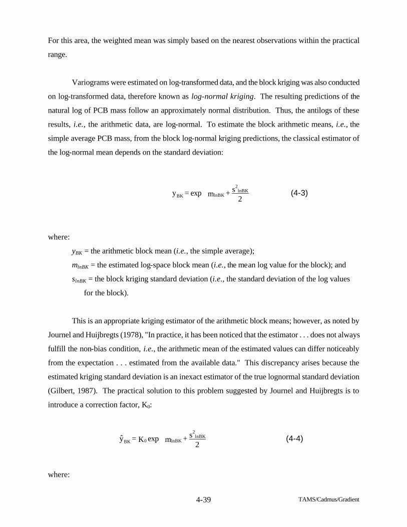
TAMS/Cadmus/Gradient 4-39
For this area, the weighted mean was simply based on the nearest observations within the practical
range.
Variograms were estimated on log-transformed data, and the block kriging was also conducted
on log-transformed data, therefore known as log-normal kriging. The resulting predictions of the
natural log of PCB mass follow an approximately normal distribution. Thus, the antilogs of these
results, i.e., the arithmetic data, are log-normal. To estimate the block arithmetic means, i.e., the
simple average PCB mass, from the block log-normal kriging predictions, the classical estimator of
the log-normal mean depends on the standard deviation:
where:
yBK = the arithmetic block mean (i.e., the simple average);
mlnBK = the estimated log-space block mean (i.e., the mean log value for the block); and
slnBK = the block kriging standard deviation (i.e., the standard deviation of the log values
for the block).
This is an appropriate kriging estimator of the arithmetic block means; however, as noted by
Journel and Huijbregts (1978), "In practice, it has been noticed that the estimator . . . does not always
fulfill the non-bias condition, i.e., the arithmetic mean of the estimated values can differ noticeably
from the expectation . . . estimated from the available data." This discrepancy arises because the
estimated kriging standard deviation is an inexact estimator of the true lognormal standard deviation
(Gilbert, 1987). The practical solution to this problem suggested by Journel and Huijbregts is to
introduce a correction factor, K0:
where:
2s + m exp = y
2lnBK
lnBKBK (4-3)
2s + m exp K = y
2lnBK
lnBK0BK (4-4)
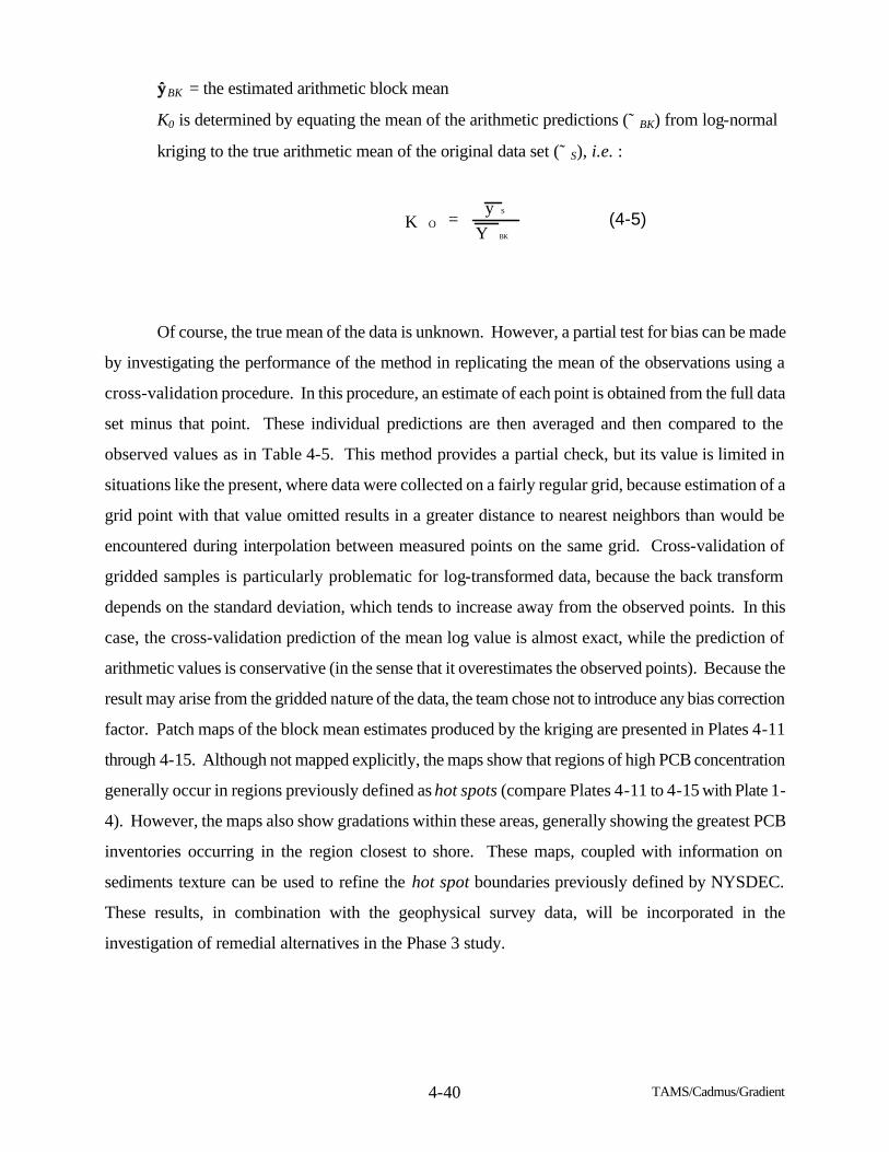
TAMS/Cadmus/Gradient 4-40
ííBK = the estimated arithmetic block mean
K0 is determined by equating the mean of the arithmetic predictions (˜BK) from log-normal
kriging to the true arithmetic mean of the original data set (˜S), i.e. :
Of course, the true mean of the data is unknown. However, a partial test for bias can be made
by investigating the performance of the method in replicating the mean of the observations using a
cross-validation procedure. In this procedure, an estimate of each point is obtained from the full data
set minus that point. These individual predictions are then averaged and then compared to the
observed values as in Table 4-5. This method provides a partial check, but its value is limited in
situations like the present, where data were collected on a fairly regular grid, because estimation of a
grid point with that value omitted results in a greater distance to nearest neighbors than would be
encountered during interpolation between measured points on the same grid. Cross-validation of
gridded samples is particularly problematic for log-transformed data, because the back transform
depends on the standard deviation, which tends to increase away from the observed points. In this
case, the cross-validation prediction of the mean log value is almost exact, while the prediction of
arithmetic values is conservative (in the sense that it overestimates the observed points). Because the
result may arise from the gridded nature of the data, the team chose not to introduce any bias correction
factor. Patch maps of the block mean estimates produced by the kriging are presented in Plates 4-11
through 4-15. Although not mapped explicitly, the maps show that regions of high PCB concentration
generally occur in regions previously defined as hot spots (compare Plates 4-11 to 4-15 with Plate 1-
4). However, the maps also show gradations within these areas, generally showing the greatest PCB
inventories occurring in the region closest to shore. These maps, coupled with information on
sediments texture can be used to refine the hot spot boundaries previously defined by NYSDEC.
These results, in combination with the geophysical survey data, will be incorporated in the
investigation of remedial alternatives in the Phase 3 study.
BK
S
Y
y = K O (4-5)
TAMS/Cadmus/Gradient 4-41
4.2.6 Kriged Total Mass Estimate
The results of the previous section were used to produce an estimate of total PCB mass in the
Thompson Island Pool as of the 1984 survey. The total mass of PCBs calculated by block kriging
(without any correction for bias) is 14.5 metric tons, with a mean mass concentration of 7.1 g/m2. This
can be compared to the estimate of M. Brown et al. (1988) of 23.2 metric tons total PCBs, with mass
concentration of 11.7 g/m2. The kriging estimate is 38 percent less than the estimate of M.
Brown et al., with a difference of 8.7 metric tons. The polygonal declustering results (Section 4.2.3)
are intermediate to the kriging estimate and the estimate reported by M. Brown et al. These estimates
differ for several reasons:
First, the estimates presented here employed a different representation of the GC/MS screening
data than was used by M. Brown et al., with uniformly lower concentration estimates. Experiments
with alternative formulations indicate that this is the major component of the difference in estimates.
The treatment of the screening data affects both the estimate of mass at individual points and the
variogram fit, both of which affect the total mass estimate.
A second component in the difference in total mass estimates is the method of spatial
interpolation. That is, in the method used by M. Brown et al., all points within a given polygon
receive equal weight. However, the sampling transects were designed to focus on suspected
hot spots, with the result that sampling density was greater in more contaminated areas. Block kriging
explicitly corrects the weighting received by each point. M. Brown et al.=s methods do so only in an
approximate, subjective manner by the assignment of polygon boundaries. In polygonal declustering,
each polygon contains a single point, and isolated, high mass estimates will be averaged over a greater
area than in the kriging approach. The different estimates vary substantially in the amount of mass
attributed to concentration classes greater than 20 g/m2. This means that the area attributed to isolated
high mass concentration measurements is less under the block kriging approach.
TAMS/Cadmus/Gradient 4-42
4.2.7 Surface Sediment PCB Concentrations
Geostatistical methods were also used to develop interpolated maps of 1984 PCB
concentrations in the near-surface layer of sediment. The surface layer is directly connected with the
water column and food chain. Spatial heterogeneity in this layer is an important consideration in the
development of bioaccumulation models. The 1984 study allows some inferences regarding the
distribution of PCBs in near-surface sediment. However, the resolution is rather coarse, as the data
provide an estimate in the uppermost sampling layer, and not true at-surface concentrations.
The grab samples are thought to represent sediments to a mean depth of approximately 12.2 inches in
gravel and 16.9 inches in finer sediments, while the upper sections of cores have a mean depth of 9.3
inches. Thus, the concentrations utilized in this analysis can be thought of as roughly equivalent to an
average in the top foot of sediment.
The intentions of the surface concentration analyses are qualitatively different than those of the
analysis of PCB mass presented above; rather than an exhaustive mean, the goal is establishing a good
map of the spatial distribution. This requires an interpolation from the measured points to unmeasured
areas. There are many ways in which this interpolation could be accomplished, including graphical
methods that interpolate contours directly between observed points. However, graphical methods are
not very satisfactory for the 1984 data for two reasons. First, it is not clear how to incorporate the
additional, but inexact, information contained in the GC/MS screening data in this approach. The
surface layer of many sample points is represented by a categorical GC/MS screening estimate, rather
than a quantitative GC/ECD estimate. Second, it is clear that there is a large degree of local
heterogeneity in the concentration measurements, attributable to both true heterogeneity in the
environment and noise introduced by imprecise laboratory determinations. Since the reported values
may not be exact or representative, an exact interpolation between nearest points is undesirable; rather
the interpolation should be based on a weighted average which takes into account the sum of evidence
of all the nearby points.
The kriging methodology described below (i.e., co-kriging) satisfies these objectives. First,
it enables incorporation of the screening data into the analysis without requiring that these be treated
as precise values for interpolation. Second, it enables estimates in unsampled areas based on an
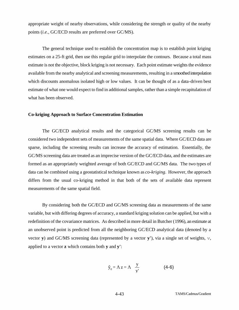
TAMS/Cadmus/Gradient 4-43
appropriate weight of nearby observations, while considering the strength or quality of the nearby
points (i.e., GC/ECD results are preferred over GC/MS).
The general technique used to establish the concentration map is to establish point kriging
estimates on a 25-ft grid, then use this regular grid to interpolate the contours. Because a total mass
estimate is not the objective, block kriging is not necessary. Each point estimate weights the evidence
available from the nearby analytical and screening measurements, resulting in a smoothed interpolation
which discounts anomalous isolated high or low values. It can be thought of as a data-driven best
estimate of what one would expect to find in additional samples, rather than a simple recapitulation of
what has been observed.
Co-kriging Approach to Surface Concentration Estimation
The GC/ECD analytical results and the categorical GC/MS screening results can be
considered two independent sets of measurements of the same spatial data. Where GC/ECD data are
sparse, including the screening results can increase the accuracy of estimation. Essentially, the
GC/MS screening data are treated as an imprecise version of the GC/ECD data, and the estimates are
formed as an appropriately weighted average of both GC/ECD and GC/MS data. The two types of
data can be combined using a geostatistical technique known as co-kriging. However, the approach
differs from the usual co-kriging method in that both of the sets of available data represent
measurements of the same spatial field.
By considering both the GC/ECD and GC/MS screening data as measurements of the same
variable, but with differing degrees of accuracy, a standard kriging solution can be applied, but with a
redefinition of the covariance matrices. As described in more detail in Butcher (1996), an estimate at
an unobserved point is predicted from all the neighboring GC/ECD analytical data (denoted by a
vector y) and GC/MS screening data (represented by a vector y'), via a single set of weights, v,
applied to a vector z which contains both y and y':
′
ΛΛ y
y = z = y0 (4-6)
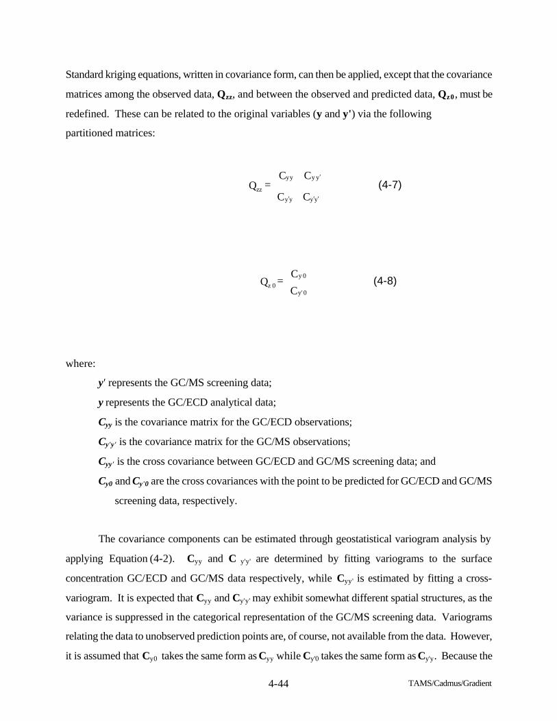
TAMS/Cadmus/Gradient 4-44
Standard kriging equations, written in covariance form, can then be applied, except that the covariance
matrices among the observed data, Qzz, and between the observed and predicted data, Qz 0 , must be
redefined. These can be related to the original variables (y and y') via the following
partitioned matrices:
where:
y' represents the GC/MS screening data;
y represents the GC/ECD analytical data;
Cyy is the covariance matrix for the GC/ECD observations;
Cy'y' is the covariance matrix for the GC/MS observations;
Cyy' is the cross covariance between GC/ECD and GC/MS screening data; and
Cy0 and Cy'0 are the cross covariances with the point to be predicted for GC/ECD and GC/MS
screening data, respectively.
The covariance components can be estimated through geostatistical variogram analysis by
applying Equation (4-2). Cyy and C y'y' are determined by fitting variograms to the surface
concentration GC/ECD and GC/MS data respectively, while Cyy' is estimated by fitting a cross-
variogram. It is expected that Cyy and Cy'y' may exhibit somewhat different spatial structures, as the
variance is suppressed in the categorical representation of the GC/MS screening data. Variograms
relating the data to unobserved prediction points are, of course, not available from the data. However,
it is assumed that Cy0 takes the same form as Cyy while Cy'0 takes the same form as Cy'y. Because the
′′′
′
CC
CC = Q
yyyy
yyyy
zz (4-7)
′C
C = Q
0 y
0y
0 z (4-8)
TAMS/Cadmus/Gradient 4-45
GC/MS results are available only as a categorical representation of the true value, they are not very
accurate predictors of y0. This is reflected in the variograms by relatively weaker correlation
between GC/MS observations and GC/ECD observations than among GC/ECD observations
themselves.
As in kriging for total mass, kriging for surface concentrations is best carried out in log space,
due to the highly skewed nature of the observed data. Because back-transforming to an arithmetic
estimate involves the estimate of the kriging variance, arithmetic estimates are sensitive to the
estimation of the ordinary kriging variance, and the unbiased correction method of Cressie (1991) was
applied.
Variogram Analysis for Surface Concentrations
For the concentration analysis, GC/MS screening categories were represented by the same
estimates used in the PCB mass calculations as shown in Table 4-2. Where sample locations were
duplicated, the data were averaged if multiple analyses of the same type were available. However,
unlike data preparation for total mass analysis, no preference was attributed to cores over grabs.
After processing duplicates and eliminating two points for which coordinates were not available, a
total of 1458 data points at 1095 locations were available for kriging, including 549 GC/ECD and
909 GC/MS measurements.
The complete sets of surface GC/ECD analytical and GC/MS screening data were used to
estimate variograms. In the subsequent kriging analysis, however, only those screening data
representing locations for which GC/ECD data were not available were retained, as the imprecise
GC/MS screening data provide a valuable addition to the estimation process only where an analytical
GC/ECD value was not available.
For variogram analysis of the GC analytical surface concentrations in log space, treatment of
nondetect values (reported as zeros in the database) is of particular importance. There are 31 of these
zero values, representing nearly 6 percent of the surface GC data. This is a sufficiently large
proportion that the representation of the nondetects has a significant effect on the estimate of the
TAMS/Cadmus/Gradient 4-46
variogram and variance of the log-transformed GC/ECD data, which in turn affects the back-
transformation to arithmetic estimates.
As discussed in Subsection 4.2.1, there is no clear specification of detection or quantitation
limit for the total PCB concentration values, although the two lowest reported detections are 0.3 and
0.5 mg/kg (300 and 500 µg/kg). When the 31 surface concentration nondetects were simply eliminated
from the dataset, the logs of the remaining values had a variance of 1.71. Analysis of variograms was
carried out with the nondetects set to several different levels for comparative purposes. In each case,
variograms of similar shape and range, but different scales on the vertical axes, were fit. Accordingly,
the variogram shape and range were fit on the data with nondetects removed. However, the scale of
the variogram was then adjusted upward by an inflation factor to represent the estimated true variance.
The unknown detection limit was assumed to be approximately 0.1 mg/kg (100 µg/kg). Based on this
assumption, the maximum likelihood estimator of the true variance of the log-transformed data,
assuming a normal distribution after transformation (Gilbert, 1987), was determined to be 2.36. This
implies the need to increase the variogram scale by the ratio of the variances or an adjustment factor of
2.36/1.71 = 1.38.
Unlike the total mass data, no clear indication of variogram anisotropy was found for either the
GC/ECD or GC/MS surface concentration data. Further, variogram analysis was not improved by
considering subreaches of the river separately. This suggests that the near-surface PCB concentration
as of 1984 was not as simply linked to river flow patterns as the total mass. Surface concentration is
presumably a function of both the mass present and local rates of deposition or scour.
Because anisotropy was not found, an omnidirectional variogram was fit to the full data set for
each type of sample. The semi-variogram for the GC/MS screening data (see Figure 4-14) showed a
strong long-range structure, with a practical range of about 750 ft, but, not surprisingly, did not yield a
sharply focused model of local-scale variability. The GC/ECD data (see Figure 4-15) suggested a
strong short-range correlation structure (with a practical range of about 125 ft), and a weaker
long-range structure (also with a practical range of less than 750 ft). The long-range structure for the
GC/ECD data reflects that seen in the screening data. To represent the GC/ECD data semi-variogram
accurately, two exponential variogram structures (plus a nugget) were required, corresponding to the
two correlation ranges in the GC/ECD data. The co-kriging method also required a cross-variogram
TAMS/Cadmus/Gradient 4-47
between GC/ECD and GC/MS data. This should reflect the structure of both semi-variograms, in
terms of correlation range, but also involves the unknown spatial pattern of the deviations of the
GC/MS categorical estimates from their true value. The cross-variogram was found to be largely a
nugget effect, with rather weak spatial correlation (see Figure 4-16). Finally, the representation of
GC/ECD nondetects also affects the estimation of the cross-variogram. In this case the adjustment
factor is the square root of that used for the GC/ECD variogram, although the solution is not very
sensitive to small errors in the cross-variogram. The variogram models determined by the procedures
above are given in Table 4-6.
Surface Kriging Results
The team used the fitted variograms and co-kriging methodology to generate point kriging
estimates of surface concentrations. Kriging was restricted to interpolation on a maximum of
12 nearest neighbors within the practical range. These neighbors might be either GC/ECD or GC/MS
screening points; however, when both GC/ECD and screening observations were available for the
same location, only the GC/ECD measurement was used. This results in estimates in some of the
intensively sampled hot spots being interpolated almost entirely on the GC/ECD data, while estimates
in some of the less intensively sampled areas depend heavily on the screening data. Estimates in these
areas are thus highly sensitive for the point representations chosen for GC/MS screening categories.
The GIS was used to produce contours from the gridded estimates using simple triangular
interpolation. The resulting maps are displayed in Plates 4-16 through 4-20. These maps will be used
in subsequent ecological, and human health impact analyses. Summary results are provided in
Table 4-7. The average surface layer concentration estimate of 28.7 mg/kg (28,700 Fg/kg) reflects
both uncontaminated areas and hot spots. It should be noted that the surface concentration estimates
are not directly comparable to mass estimates. This is because of a strong inverse correlation
between concentration and specific weight, with highest PCB concentrations associated with lower
specific weights.
A cross-validation analysis was performed to look for potential bias in the kriged estimates of
surface PCB concentration. This analysis was performed in a similar manner to that for the PCB mass
estimates, i.e., estimates were generated for each sampling location, excluding the value measured at
the specific location. Cross-validation suggests that the surface concentration estimates are in the
TAMS/Cadmus/Gradient 4-48
range expected from the data. Elevated surface PCB concentrations generally correlated well with
NYSDEC hot spot boundaries, as expected. The observed GC/ECD measurements, which focus on
hot spots, have a mean of 56.0 ppm, while the GC/MS data have an estimated mean of 19.8 ppm, with
greater coverage of less contaminated areas. Cross-validated estimates of all observed points as a
group have a mean of 41.7 ppm, representing a shift from the GC/ECD mean toward the GC/MS mean.
4.2.8 Summary
• Two estimates were made of the PCB inventory sequestered in the sediments of the TIP, as
of 1984. The first estimate, based on a technique called polygonal declustering, yielded an
estimate of 19.6 metric tons, 16 percent lower than the original estimate of 23.2 metric
tons by M. Brown et al., 1984. The second, based on a kriging analysis, yielded an
estimate of 14.5 metric tons, 38 percent lower than the estimate by M. Brown et al.
• The lower PCB inventory estimates obtained in the Phase 2 analysis were attributed to two
factors. First, the Phase 2 analysis used median value estimates rather than the mean value
estimates used by NYSDEC assessing the GC/MS screening data. The second reason for
the lower estimate obtained by the kriging analysis was attributed to the spatial
interpolation to unsampled locations inherent in the kriging technique. This approach
should provide improved estimates of PCB mass contained in under-sampled sections of
the Thompson Island Pool.
• A series of plates (maps) was created representing the Phase 2 estimates spatially and
shows, as expected, the correlation of NYSDEC hot spots with areas of high PCB
inventories. These maps will provide a basis for estimation of sediment volume in
evaluating remedial alternatives.
• The assumptions used by M. Brown et al., 1988, were reviewed and critiqued.
• The specific weight data obtained by NYSDEC may be biased high and thus serve to bias
the PCB mass estimates high. However, no better basis to estimate this parameter exists
and so the current analysis is based on the same values used by NYSDEC.
TAMS/Cadmus/Gradient 4-49
• Surface PCB concentrations were assessed in a similar, but not identical, kriging analysis.
Maps of contoured PCB concentrations were produced based on this analysis. These
maps will be used in subsequent ecological, and human health impact analyses.
• Elevated surface PCB concentrations generally correlated well with NYSDEC hot spot
boundaries, as expected.
4.3 PCB Fate in Sediments of the Hudson River
PCBs are sequestered within the sediments of the Hudson River as suspended matter settles to
the bottom. Once deposited, these PCBs may be affected by a number of processes, including
remobilization, biogeochemical transformations, degradation, and burial. Because of the long history
of PCB contamination, an extensive inventory of PCBs has been sequestered in the sediments of the
Hudson River (Bopp, 1979; Tofflemire, 1980; Malcolm Pirnie, Inc., 1984; Bopp et al., 1985; M.
Brown, et al. 1988). Remobilization by sediment resuspension or porewater displacement can serve
to return PCBs to the water column long after any point source contributions have been eliminated.
Thus the fate of the PCBs within the sediments becomes important when considering the long-term
recovery of the river.
In the previous two sections of this chapter, the discussions centered on establishing those
areas where sediment PCB concentrations are high and potentially of concern. This section will
address the fate of the PCBs within the contaminated sediment itself. This section discusses the results
of the Phase 2 high-resolution sediment coring program for the purpose of examining the fate of PCBs
within the sediments. This interpretation is based in part on the results of the dating techniques
discussed in Subsection 3.3.1. The congener-specific analytical techniques outlined in Section 1.4
were applied to the high-resolution sediment cores discussed here and provide the basis for the
interpretations which follow.
4.3.1 Anaerobic Dechlorination and Aerobic Degradation
TAMS/Cadmus/Gradient 4-50
Before discussing the findings of the Phase 2 investigation, it is necessary to define the terms
used in the discussion below. Alteration of PCBs within the sediments can occur under both aerobic
and anaerobic conditions. Processes affecting PCBs under both conditions have the potential to alter
the inventory of PCBs within the sediments. Destruction of PCBs occurs only when a chlorinated
biphenyl molecule ceases to exist. Dechlorination is the chemical process of removing one or more
chlorine atoms from a chemical structure, in this case a polychlorinated biphenyl (PCB) molecule,
while degradation is defined as the destruction of the PCB molecule into products which do not
contain chlorinated biphenyl. Figure 4-17 is a representation of a typical PCB molecule showing
several chlorine atoms on the main biphenyl structure. On a simple theoretical basis, dechlorination
can destroy a PCB molecule by removing all chlorine atoms from the biphenyl structure.
Several investigators have demonstrated the occurrence and mechanisms of PCB destruction
under aerobic conditions (e.g., Furukawa, 1982; Bedard et al., 1987; Bedard, 1990; Abramowicz and
Brennan, 1991). In these instances, the PCB molecules are generally destroyed via the destruction of
the biphenyl structure, not by the cleavage of chlorine atoms. For the purposes of this discussion,
these processes can be grouped under the term aerobic degradation. In general, these aerobic
processes affect only the lightest congeners, monochloro- to trichlorobiphenyls, and are ineffective at
altering heavy congeners (those with four or more chlorine atoms) under environmental conditions.
Similarly, several investigations have shown that some PCB congeners can be dechlorinated by
microorganisms in an anaerobic environment (e.g., J. Brown et al., 1984; J. Brown et al., 1987; Rhee
et al., 1993a; and Rhee et al., 1993b). Reductive dechlorination of PCBs by microorganisms from the
Hudson River occurs anaerobically, i.e., in the absence of oxygen, primarily through the removal of
the meta-chlorines and, to a lesser extent, the para-chlorines in PCBs bound to subsurface sediments
(Rhee et al., 1993b; Quensen et al., 1990). A meta-chlorine is bound to the third or fifth position in
the biphenyl molecule, while a para-chlorine is bound in the fourth position. A chlorine atom located
in the second or sixth position on the biphenyl ring is labeled an ortho-chlorine. Figure 4-17 shows
these positions on the biphenyl molecule. The dechlorination process is more effective on the heavier
PCB homologues, in which meta- and para-chlorines occur frequently.
The process of dechlorination has the net effect of reducing the mass of PCBs within the
sediments without reducing the total molecular PCB concentration unless the process removes all
chlorine atoms. Thus, by dechlorination a hexachlorobiphenyl molecule may be converted to a
TAMS/Cadmus/Gradient 4-51
trichlorobiphenyl molecule but the same number of chlorinated biphenyl molecules remain in the
sediments. Only if all chlorine atoms are removed does this process actually destroy PCBs. The
dechlorination process largely serves to change the nature of the PCBs within the sediments, affecting
both the geochemical and toxicological properties of the mixture. In general, dechlorination converts
the PCBs to a more soluble form, with a lower sediment-to-water partition coefficient as discussed in
Section 3.1. These lesser chlorinated PCB congeners may become more susceptible to aerobic
degradation if the PCB bearing sediments are re-exposed to aerobic conditions. The changes in the
toxicological properties are less certain. Based on the laboratory toxicities of various Aroclor
mixtures, more-chlorinated congeners are more often associated with carcinogenic endpoints while the
literature suggests that less-chlorinated congeners are more likely to produce neurological impairment
and developmental damage (Eastern Research Group, Inc., 1993; Barnes et al.,1991). Thus,
depending upon the route of exposure and the human receptor, the dechlorination process may not
serve to reduce the net human health impact, as might be anticipated.
As discussed previously, laboratory studies have shown that several PCB congeners can be
degraded aerobically by some bacterial strains. J. Brown (1993 and 1994) cites evidence of aerobic
degradation in the surface water of the Hudson River. However, the majority of the PCB inventory in
the Hudson River lies within anaerobic sediments. To date, little evidence has been demonstrated for
anaerobic degradation in sediments, i.e., the destruction of the PCB molecule under anaerobic
conditions. In the remainder of this section, the discussion will focus on the evidence for the long-
term fate of PCBs in the environment obtained during the Phase 2 investigation. In particular,
evidence for anaerobic dechlorination will be presented. The issue of anaerobic destruction of PCBs
will also be discussed here based on the high resolution sediment core results, but further discussion
will follow in a Phase 3 report incorporating the results of both the low and high resolution coring
programs.
TAMS/Cadmus/Gradient 4-52
4.3.2 Anaerobic Dechlorination as Documented in Phase 2 High-Resolution Sediment
Cores
Evidence for anaerobic dechlorination was obtained from the results of the high-resolution
sediment coring program. The cores were used in this examination since they provide a broad range
of PCB concentrations as well as information on the age of the sediment deposits. A substantial
number of sediment-core samples contained high levels of specific PCB congeners considered to be
products of this process. These results were used along with other data to examine the degree of PCB
dechlorination in the sediments and the potentially important factors controlling this phenomenon.
Based on this analysis, it is concluded that the degree of in situ PCB dechlorination is not a function of
time but rather dependent upon the total PCB concentration within the sediment. In addition, the ability
of the dechlorination process to remove PCB mass is quite limited, due to the resistance of
ortho-chlorines to removal.
Assessing the Degree of Dechlorination
Estimates of the degree of in situ alteration, e.g., anaerobic dechlorination, of the PCB mixture
in the sediment must be predicated on some knowledge of the types of PCB mixtures present in the
environment at the time of sediment deposition. Using this knowledge, the ratio of dechlorination
products relative to the original congener mixture can be used as a measure of the degree of
dechlorination resulting from PCB storage within the sediments. Fortunately, this information can be
inferred from two sources. The PCB usage at the GE facilities has been documented and is presented
in detail in Section B.2 of the Phase 1 Report (TAMS/Gradient, 1991).
To briefly summarize the reported GE PCB usage, the mixture used at their facilities from
1945 to the mid-1950s was principally Aroclor 1254 with some Aroclor 1242, representing a
relatively more-chlorinated mixture of congeners. Aroclor 1242, a less-chlorinated mixture,
represented more than 95 percent of the usage from 1955 to 1971. From 1971 through 1977, Aroclor
1242 usage was replaced with Aroclor 1016, which represented essentially 100 percent of the
reported usage during this period. Aroclor 1016 differs only marginally from Aroclor 1242, the
TAMS/Cadmus/Gradient 4-53
difference being that congeners above BZ#56 are greatly reduced in Aroclor 1016 relative to Aroclor
1242. Integrating the entire period of operation, Aroclor 1242 was the principal congener mixture
based on tonnage used.
There are no records describing the mixture of PCBs released from the GE facilities to the
environment, but presumably the mixtures released would represent some combination of those in use
at the facilities at the time of release. The possibility exists that both pure product and altered Aroclor
mixtures resulting from the manufacturing process were released into the river. However, all available
monitoring evidence indicates that the principal PCB mixture released by GE was unaltered Aroclor
1242 and that this release dominated the PCB loading to the entire freshwater Hudson. Section 3.2
and Subsection 3.3.3 of this report and GE's 1992 Remnant Deposit Monitoring Report (O'Brien &
Gere, 1993a) indicate that 1991 to 1993 loadings at Rogers Island were largely unaltered Aroclor
1242, the principal Aroclor used at the facilities. Dated sediment cores collected by Bopp and others
(Bopp et al., 1982; and Bopp and Simpson, 1989) show the PCB mixture in sediments in the
freshwater Hudson to be principally derived from Aroclor 1242 during the period 1954 to the
mid-1980s. The dated sediment core analysis presented in Subsection 3.3.3 shows the combined
Thompson Island Dam load to represent the major load to the entire freshwater Hudson for the period
1975 to 1992. Based on this information, Aroclor 1242 was assumed to be the principal congener
mixture sequestered in the sediments over the period 1954 to 1992.
The extent of dechlorination was examined by two different approaches. The first approach
was based on measured concentrations of several congeners believed to represent final or near-final
dechlorination products, specifically, BZ#1 (2-monochlorobiphenyl), BZ#4 (2,2'-dichlorobiphenyl),
BZ#8 (2,4=-dichlorobiphenyl), BZ#10 (2,6-dichlorobiphenyl), and BZ#19 (2,2',6-trichlorobiphenyl).
The second approach examined the change in the mean molecular weight of the PCBs in a sample. It
should be noted that BZ#8 was included as a Anear final@ dechlorination product based on the Phase 2
results. It is clearly not a final product in that it can lose its one para-chlorine and form BZ#1.
However, its concentration relative to other congeners in many sediment samples clearly indicate its
status as a dechlorination product. While most other congeners in the sediment samples tended to be at
or below their mass fractions relative to unaltered Aroclor 1242, BZ#8 was frequently well above it,
sometimes as much as three times greater. Based on this observation, BZ#8 was included as a
dechlorination product. Also note that there is one additional congener, BZ#54, (2,2',6,6'-
TAMS/Cadmus/Gradient 4-54
tetrachlorobiphenyl) which consists solely of ortho-substituted chlorines. BZ#54 was not a reported
analyte in the Phase 2 program.
All freshwater core results collected in Phase 2 were included in this examination. The core
results were split into three groups, i.e., background and tributaries; Upper Hudson; and Lower
Hudson. The background and tributaries group includes cores from the Mohawk, Hoosic and Batten
Kill as well as the core collected at RM 202.7, upstream of the GE releases. The Upper Hudson
group contains all cores between RM 198 and RM 157, representing Upper Hudson sediments at or
downstream of the GE facilities. The Lower Hudson group includes all core results between RM 157
and RM 88, representing freshwater sediments in the Lower Hudson. Although these sediment cores
cannot be used to estimate sediment PCB inventories over large areas, they can be used to represent
the in situ conditions to which PCBs are generally subjected. Thus they can provide a measure of the
degree of alteration expected in other PCB-bearing sediments. As an initial screening, PCB results
were selected only from those sediments containing measurable amounts of 137Cs. 137Cs-bearing
sediments are considered to represent post-1954 deposition (see Subsection 3.3.1). Given the
temporal resolution of the sediment core samples, typically to within about two years, 1954 also
corresponds closely to the onset of major Aroclor 1242 usage at the GE facilities in 1955. A subset of
the cores, specifically the datable sediment cores, was examined to assess the time-dependence of the
in situ alterations measured in greater detail.
TAMS/Cadmus/Gradient 4-55
Examination of the Dechlorination Products
The first approach to examining the extent of dechlorination involved measuring the
concentration of several congeners that are exclusively ortho-substituted and are not believed to be
subject to further dechlorination. Abramowicz et al. (1993) found that no ortho-dechlorination was
detected in a laboratory study using Hudson River sediments and that less-chlorinated, ortho-enriched
congeners accumulated. The study states "ortho dechlorination has never been reported with Hudson
River sediments." Quensen et al. (1990) obtained a similar finding concerning the stability of
ortho-chlorine atoms. On this basis, the five exclusively ortho-substituted congeners (BZ#1, 4, 10, 19,
and 54) can be considered ultimate dechlorination products (i.e., dechlorination products containing
only ortho-substituted chlorine atoms and not susceptible to further dechlorination). Of these five
congeners, four (BZ#1, 4, 10 and 19) were quantitated by the Phase 2 PCB analytical method. As
noted previously, a sixth congener, BZ#8 (2,4'-dichlorobiphenyl), appears to be a significant
dechlorination product, possibly an intermediate. This congener exhibited greatly increased
concentrations relative to other Aroclor 1242 components, suggesting its production within the
sediments. There are undoubtedly other dechlorination products, including other intermediates subject
to further dechlorination, but their transient nature makes them more difficult to use in this analysis.
Limiting the subsequent analysis to just the four ortho-substituted congeners (BZ#1, 4, 10, and 19) plus
BZ#8, provides a lower bound on the portion of the sediment PCB content which has undergone some
degree of dechlorination.
Because dechlorination does not modify the biphenyl structure of a PCB molecule, it was
assumed that the biphenyl structure would be conserved for those PCB congeners containing at least
one ortho-chlorine; i.e., in the absence of other losses, the total molar concentration of ortho-
substituted PCBs in the sediments would be conserved. Thus the extent of dechlorination can be
measured as the molar ratio of the ultimate dechlorination products to the total molar PCB
concentration of ortho-substituted congeners, i.e., the ratio of altered molecules to the original number
of molecules. Instead of considering only ortho-substituted congeners, this ratio was modified to
include all measured congeners to simplify its calculation. Since the vast majority of PCB congeners
found in Aroclor 1242 contain at least one ortho-chlorine (75 out of the 82 congeners detected in an
Aroclor 1242 standard, representing 95.5 percent of the mass of unaltered Aroclor 1242), this
TAMS/Cadmus/Gradient 4-56
simplification does not introduce a significant underestimate of the degree of alteration for most
Hudson River sediments. Table 4-8 lists the 82 congeners detected in an Aroclor 1242 standard by
the Phase 2 analytical method along with their ultimate dechlorination product. The ratio of the sum of
the five congener molar concentrations (BZ# 1+4+8+10+19) to the total sample molar concentration
will be referred to as the molar dechlorination product ratio (MDPR) in subsequent discussions and
is calculated as follows:
where:
[BZ#i], [BZ#j] are the molar concentration of the congener in the sample (mole/kg); and
126 is the number of congeners for which consistent reliable identification and quantitative
data were generated in the Phase 2 analytical program. Note that these 126 congeners
represent all of the homologue groups as shown in Table 1-4.
Since dechlorination produces lighter molecules, more readily soluble and possibly more susceptible
to other degradation processes, estimating the extent of dechlorination by this ratio probably
represents a slight underestimate of the actual degree of dechlorination.
The initial MDPRs of the three Aroclors used by General Electric (i.e., Aroclors 1242, 1254,
and 1016) are 0.17 or less based on Phase 2 analyses of commercially available Aroclor standards.
Figure 4-18 shows the congener composition of the three standard Aroclor mixtures. (Aroclor 1260 is
also shown in the figure for comparison.) Table 4-9 lists the individual mole fractions for each of the
five ultimate dechlorination product congeners in the three unaltered Aroclor mixtures. The
assumption that Aroclor 1242 was the principal mixture sequestered in the sediments suggests an
initial MDPR of 0.14. MDPRs greater than this value indicate the likelihood of in situ dechlorination.
In a sediment sample with an MDPR of 0.34, dechlorination has affected approximately 20 percent
(i.e., 0.34 - 0.14) of the PCB molecules. In a sample in which all possible PCB molecules have been
[BZ#j]
[BZ#i]
1=j
19 10, 8, 4, 1, = i
126 = MDPR
∑
∑ (4-9)
TAMS/Cadmus/Gradient 4-57
dechlorinated, the MDPR is 1.0, indicating that a maximum of 86 percent (i.e., 1.00 - 0.14) of PCB
molecules can theoretically be affected. In fact, however, since BZ#8 can be further dechlorinated to
BZ#1, 94.4 percent of the molecules can ultimately be affected by this process. If BZ#8 is not
included in the MDPR, the initial Aroclor 1242 value is 0.06.
It should be emphasized that MDPR is a measure of the number of affected PCB molecules and
not a mass loss measurement. Based on the evidence which indicates that ortho-chlorines cannot be
removed under anaerobic conditions and the biphenyl structure is preserved by dechlorination, there is
a theoretical limit to the PCB mass reduction which can be achieved by this process. For Aroclor
1242, which is predominantly a tri-chlorinated congener mixture, meta and para-chlorines represent
23 percent of the mass of the mixture. In a few instances, loss of these chlorines results in a
dechlorination product which is not reported in the Phase 2 database (i.e., BZ#54 or biphenyl). This
results in a maximum mass reduction by dechlorination of no more than 26.1 percent assuming that all
non-ortho-chlorines are removed by the dechlorination process. For Aroclor 1016, the maximum mass
reduction is 22 percent. For Aroclor 1254, the maximum mass reduction is 32 percent. Thus, given
the lack of ortho-chlorine removal, the dechlorination process is theoretically limited in its ability to
reduce the PCB sediment inventory.
Two issues remain concerning the use of the MDPR before evaluating the sample results:
alteration of the Aroclor mixture prior to deposition or just after deposition; and the effects of the
presence of non-ortho-substituted congeners. The alteration of the Aroclor mixture in the water column
and surficial sediments prior to reaching anaerobic conditions would be expected to reduce the
dechlorination product ratio since both suspended matter-water partitioning and aerobic degradation
generally serve to decrease the fraction of less chlorinated congeners in the sediment. Thus the MDPR
of 0.14 based on unaltered Aroclor 1242 may overestimate the MDPR of Aroclor 1242 at the time and
conditions of deposition in the (anaerobic) sediment. However, this represents a relatively small
uncertainty based on the variability of the measured results.
The second issue concerns the effects of non-ortho-substituted congeners. When these
congeners undergo dechlorination, they do not yield any of the five congeners contained in the MDPR.
In addition, these congeners have the potential to be fully degraded by dechlorination since they lack
ortho-chlorines. There are also several congeners which will form the tetra-ortho-chlorinated
TAMS/Cadmus/Gradient 4-58
congener BZ#54 (2,2=,6,6=-tetrachlorobiphenyl), a congener which is not included in the Phase 2
analytical program. In all, 18 of the 126 congeners represented in the Phase 2 PCB analysis do not
yield a measured product as a result of dechlorination, i.e., they are effectively Adestroyed@ by
dechlorination from the perspective of the Phase 2 analytical data since their presence is not reported.
However, these congeners do not represent a significant fraction of the congeners present in the three
Aroclor mixtures and therefore, their impact on the MDPR is minimal. Table 4-8 shows the mass and
molar loss calculations for Aroclor 1242. Table 4-10 summarizes the analytical results for the three
Aroclors based on the ortho-substituted congeners and those congeners whose dechlorination products
are not reported. Since the unreported portion is by definition unknown, the MDPR will have at most
a 5.0 percent bias (the mole fraction of these congeners) if all congeners with unreported
dechlorination products are completely dechlorinated. In view of the theoretical range measured
range of this ratio for Aroclor 1242 [0.86 (1.00 - 0.14)], this bias will be ignored in subsequent
discussions.
Examination of the Change in Mean Molecular Weight.
The mean molecular weight of a given Aroclor mixture (e.g., Aroclor 1242) can be determined
from a mass fraction weighted average of the individual PCB congeners comprising that Aroclor. One
of the benefits of the analytical techniques used in the Phase 2 program is the ability to quantitate the
concentrations of individual congeners. This information combined with the known molecular weight
of each congener was used to calculate a PCB mass-weighted mean molecular weight for each
freshwater sediment sample. This value was then compared with the similarly calculated molecular
weight of Aroclor 1242 as a measure of the extent of dechlorination in the sample. The fractional
difference in molecular weight between Aroclor 1242 and the sample can provide an estimate of the
mass loss which has occurred from the time of release (when the mixture was presumably unaltered
Aroclor 1242), given the assumption that PCB molecules have not been lost or destroyed. In the
absence of other PCB loss mechanisms, this measure provides an estimate of the mass lost via
dechlorination as heavier molecules are converted to lighter ones, lowering the molecular weight in
proportion to the mass lost. The fractional change in mean molecular weight was calculated as
follows:
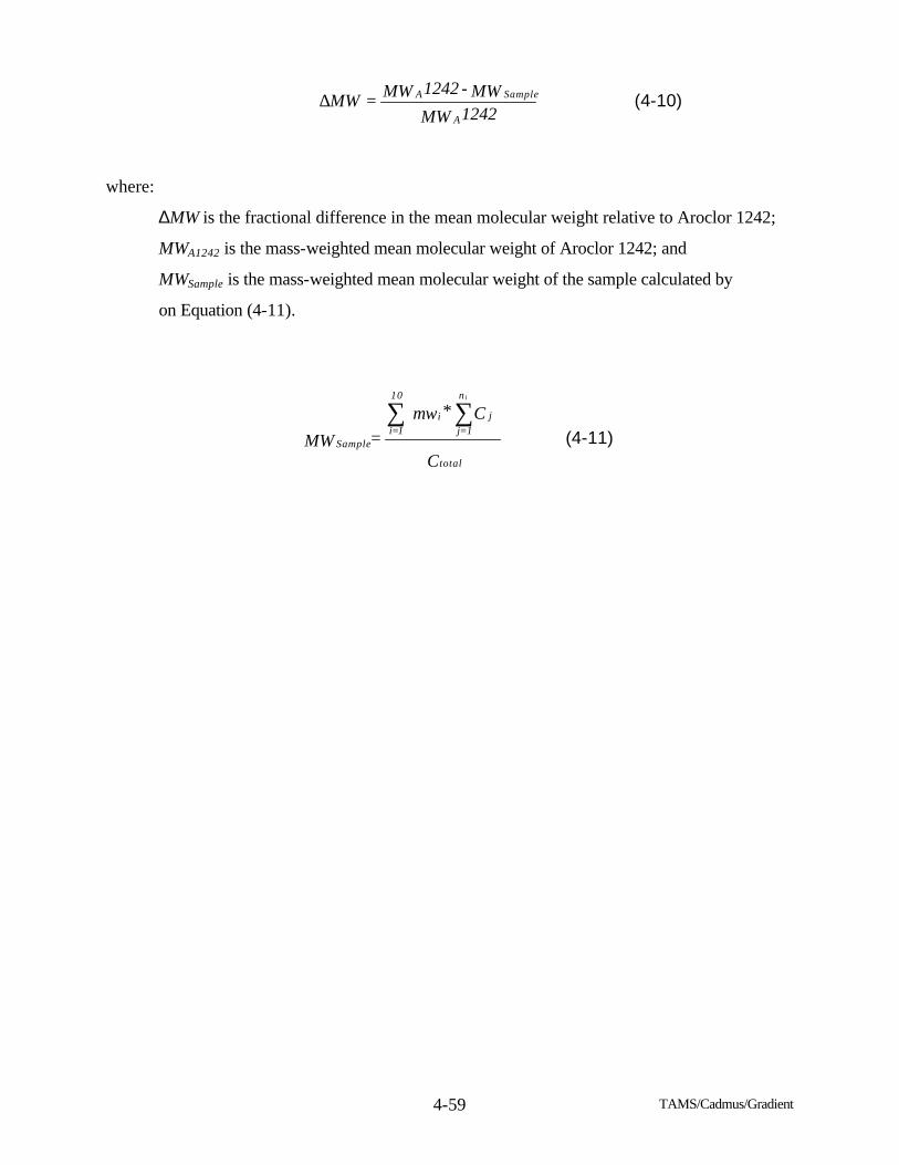
TAMS/Cadmus/Gradient 4-59
where:
∆MW is the fractional difference in the mean molecular weight relative to Aroclor 1242;
MWA1242 is the mass-weighted mean molecular weight of Aroclor 1242; and
MWSample is the mass-weighted mean molecular weight of the sample calculated by
on Equation (4-11).
MW
MW-MW=MWA1242
SampleA1242∆ (4-10)
C
C*mw
=MWtotal
j
n
1=ji
10
1=iSample
i
∑∑
(4-11)
TAMS/Cadmus/Gradient 4-60
where:
i is the homologue group number from 1 to 10;
mwi is the molecular weight of homologue group i in g/mole;
ni is the number of measured congeners in homologue group i;
Cj is the concentration of congener j in µg/kg; and
Ctotal is the total PCB concentration in the sample in µg/kg.
Note that congener mixtures with lower molecular weights than Aroclor 1242 have a positive
value for ∆MW and mixtures with higher molecular weights have a negative ∆MW.
Other loss mechanisms may also change the molecular weight. Loss of PCB molecules by
degradation processes or pore water movement can raise or lower the molecular weight of the
mixture. If lighter congeners are lost, the molecular weight increases. If heavier molecules are lost,
the molecular weight decreases. However, the mean molecular weights of Phase 2 sediment samples
with low concentrations of dechlorination products have been found to be close to that of Aroclor
1242, indicating that processes other than dechlorination have not greatly modified the sample PCB
content. This will be discussed in greater detail below.
As noted previously, there is a theoretical limit to the possible mass loss which can occur via
dechlorination, i.e., about 26 percent for Aroclor 1242 assuming no ortho-chlorine loss. As a part of
this loss, several congeners which do not yield measurable (reported) products can be lost via
dechlorination, as discussed above. The loss of these congeners represents about 4.5 percent out of
the total theoretical mass loss limit of 26.1 percent. Meta- and para-dechlorination yielding
measurable products represent the remaining 21.6 percent. However, unlike the loss of chlorine
atoms, the molecular weight change may not directly reflect these unmeasured congeners, depending
upon their molecular weight and their concentration in the unaltered Aroclor. Based on the Phase 2
Aroclor standard results, the maximum molecular weight change corresponding to the total maximum
mass loss is 22.3 percent. Thus, in the absence of other loss mechanisms, no sample should yield a
∆MW greater than 22.3 percent if meta- and para-dechlorination are the only dechlorination
mechanisms. The close agreement between the theoretical mass change (26.1 percent) and the
theoretical molecular weight change (22.3 percent) reflects the fact that Aroclor 1242, as well as the
other Aroclors discussed here, principally consist of congeners with ortho-chlorines. For example, of
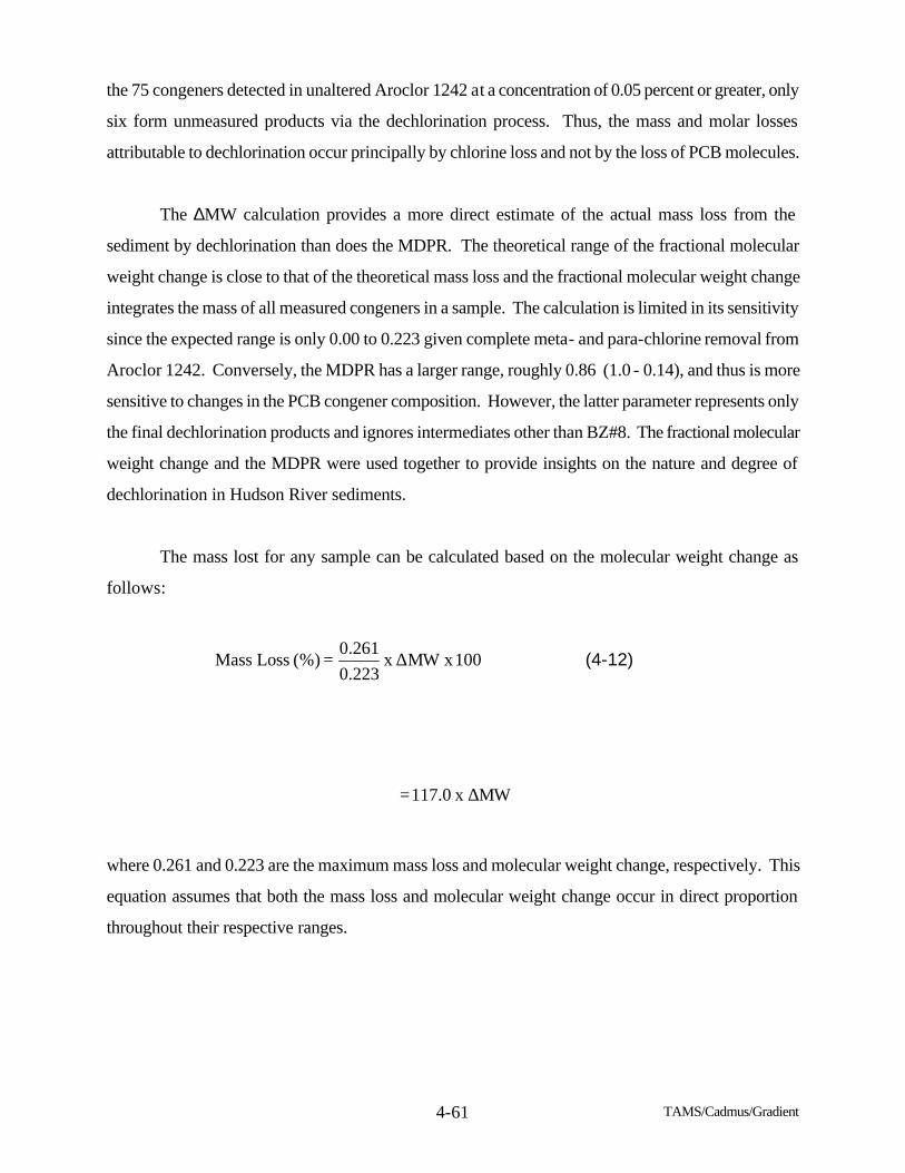
TAMS/Cadmus/Gradient 4-61
the 75 congeners detected in unaltered Aroclor 1242 at a concentration of 0.05 percent or greater, only
six form unmeasured products via the dechlorination process. Thus, the mass and molar losses
attributable to dechlorination occur principally by chlorine loss and not by the loss of PCB molecules.
The ∆MW calculation provides a more direct estimate of the actual mass loss from the
sediment by dechlorination than does the MDPR. The theoretical range of the fractional molecular
weight change is close to that of the theoretical mass loss and the fractional molecular weight change
integrates the mass of all measured congeners in a sample. The calculation is limited in its sensitivity
since the expected range is only 0.00 to 0.223 given complete meta- and para-chlorine removal from
Aroclor 1242. Conversely, the MDPR has a larger range, roughly 0.86 (1.0 - 0.14), and thus is more
sensitive to changes in the PCB congener composition. However, the latter parameter represents only
the final dechlorination products and ignores intermediates other than BZ#8. The fractional molecular
weight change and the MDPR were used together to provide insights on the nature and degree of
dechlorination in Hudson River sediments.
The mass lost for any sample can be calculated based on the molecular weight change as
follows:
where 0.261 and 0.223 are the maximum mass loss and molecular weight change, respectively. This
equation assumes that both the mass loss and molecular weight change occur in direct proportion
throughout their respective ranges.
100x MWx 0.223
0.261=(%) LossMass ∆ (4-12)
MWx 117.0 = ∆
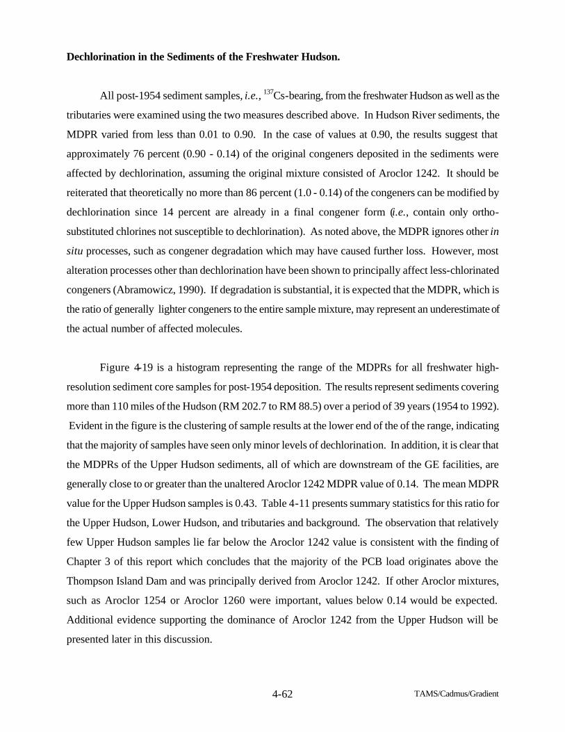
TAMS/Cadmus/Gradient 4-62
Dechlorination in the Sediments of the Freshwater Hudson.
All post-1954 sediment samples, i.e., 137Cs-bearing, from the freshwater Hudson as well as the
tributaries were examined using the two measures described above. In Hudson River sediments, the
MDPR varied from less than 0.01 to 0.90. In the case of values at 0.90, the results suggest that
approximately 76 percent (0.90 - 0.14) of the original congeners deposited in the sediments were
affected by dechlorination, assuming the original mixture consisted of Aroclor 1242. It should be
reiterated that theoretically no more than 86 percent (1.0 - 0.14) of the congeners can be modified by
dechlorination since 14 percent are already in a final congener form (i.e., contain only ortho-
substituted chlorines not susceptible to dechlorination). As noted above, the MDPR ignores other in
situ processes, such as congener degradation which may have caused further loss. However, most
alteration processes other than dechlorination have been shown to principally affect less-chlorinated
congeners (Abramowicz, 1990). If degradation is substantial, it is expected that the MDPR, which is
the ratio of generally lighter congeners to the entire sample mixture, may represent an underestimate of
the actual number of affected molecules.
Figure 4-19 is a histogram representing the range of the MDPRs for all freshwater high-
resolution sediment core samples for post-1954 deposition. The results represent sediments covering
more than 110 miles of the Hudson (RM 202.7 to RM 88.5) over a period of 39 years (1954 to 1992).
Evident in the figure is the clustering of sample results at the lower end of the of the range, indicating
that the majority of samples have seen only minor levels of dechlorination. In addition, it is clear that
the MDPRs of the Upper Hudson sediments, all of which are downstream of the GE facilities, are
generally close to or greater than the unaltered Aroclor 1242 MDPR value of 0.14. The mean MDPR
value for the Upper Hudson samples is 0.43. Table 4-11 presents summary statistics for this ratio for
the Upper Hudson, Lower Hudson, and tributaries and background. The observation that relatively
few Upper Hudson samples lie far below the Aroclor 1242 value is consistent with the finding of
Chapter 3 of this report which concludes that the majority of the PCB load originates above the
Thompson Island Dam and was principally derived from Aroclor 1242. If other Aroclor mixtures,
such as Aroclor 1254 or Aroclor 1260 were important, values below 0.14 would be expected.
Additional evidence supporting the dominance of Aroclor 1242 from the Upper Hudson will be
presented later in this discussion.
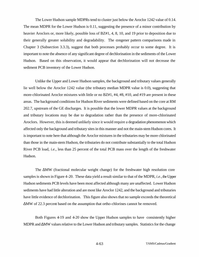
TAMS/Cadmus/Gradient 4-63
The Lower Hudson sample MDPRs tend to cluster just below the Aroclor 1242 value of 0.14.
The mean MDPR for the Lower Hudson is 0.11, suggesting the presence of a minor contribution by
heavier Aroclors or, more likely, possible loss of BZ#1, 4, 8, 10, and 19 prior to deposition due to
their generally greater solubility and degradability. The congener pattern comparisons made in
Chapter 3 (Subsection 3.3.3), suggest that both processes probably occur to some degree. It is
important to note the absence of any significant degree of dechlorination in the sediments of the Lower
Hudson. Based on this observation, it would appear that dechlorination will not decrease the
sediment PCB inventory of the Lower Hudson.
Unlike the Upper and Lower Hudson samples, the background and tributary values generally
lie well below the Aroclor 1242 value (the tributary median MDPR value is 0.0), suggesting that
more-chlorinated Aroclor mixtures with little or no BZ#1, #4, #8, #10, and #19 are present in these
areas. The background conditions for Hudson River sediments were defined based on the core at RM
202.7, upstream of the GE discharges. It is possible that the lower MDPR values at the background
and tributary locations may be due to degradation rather than the presence of more-chlorinated
Aroclors. However, this is deemed unlikely since it would require a degradation phenomenon which
affected only the background and tributary sites in this manner and not the main-stem Hudson cores. It
is important to note here that although the Aroclor mixtures in the tributaries may be more chlorinated
than those in the main-stem Hudson, the tributaries do not contribute substantially to the total Hudson
River PCB load, i.e., less than 25 percent of the total PCB mass over the length of the freshwater
Hudson.
The ∆MW (fractional molecular weight change) for the freshwater high resolution core
samples is shown in Figure 4-20. These data yield a result similar to that of the MDPR, i.e., the Upper
Hudson sediments PCB levels have been most affected although many are unaffected. Lower Hudson
sediments have had little alteration and are most like Aroclor 1242, and the background and tributaries
have little evidence of dechlorination. This figure also shows that no sample exceeds the theoretical
∆MW of 22.3 percent based on the assumption that ortho-chlorines cannot be removed.
Both Figures 4-19 and 4-20 show the Upper Hudson samples to have consistently higher
MDPR and ∆MW values relative to the Lower Hudson and tributary samples. Statistics for the change
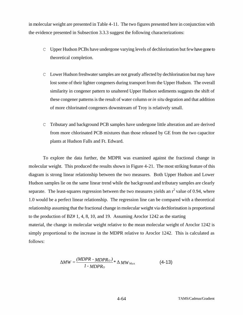
TAMS/Cadmus/Gradient 4-64
in molecular weight are presented in Table 4-11. The two figures presented here in conjunction with
the evidence presented in Subsection 3.3.3 suggest the following characterizations:
C Upper Hudson PCBs have undergone varying levels of dechlorination but few have gone to
theoretical completion.
C Lower Hudson freshwater samples are not greatly affected by dechlorination but may have
lost some of their lighter congeners during transport from the Upper Hudson. The overall
similarity in congener pattern to unaltered Upper Hudson sediments suggests the shift of
these congener patterns is the result of water column or in situ degration and that addition
of more chlorinated congeners downstream of Troy is relatively small.
C Tributary and background PCB samples have undergone little alteration and are derived
from more chlorinated PCB mixtures than those released by GE from the two capacitor
plants at Hudson Falls and Ft. Edward.
To explore the data further, the MDPR was examined against the fractional change in
molecular weight. This produced the results shown in Figure 4-21. The most striking feature of this
diagram is strong linear relationship between the two measures. Both Upper Hudson and Lower
Hudson samples lie on the same linear trend while the background and tributary samples are clearly
separate. The least-squares regression between the two measures yields an r2 value of 0.94, where
1.0 would be a perfect linear relationship. The regression line can be compared with a theoretical
relationship assuming that the fractional change in molecular weight via dechlorination is proportional
to the production of BZ# 1, 4, 8, 10, and 19. Assuming Aroclor 1242 as the starting
material, the change in molecular weight relative to the mean molecular weight of Aroclor 1242 is
simply proportional to the increase in the MDPR relative to Aroclor 1242. This is calculated as
follows:
MW * MDPR-1
)MDPR - (MDPR = MW
O
OMax∆∆ (4-13)
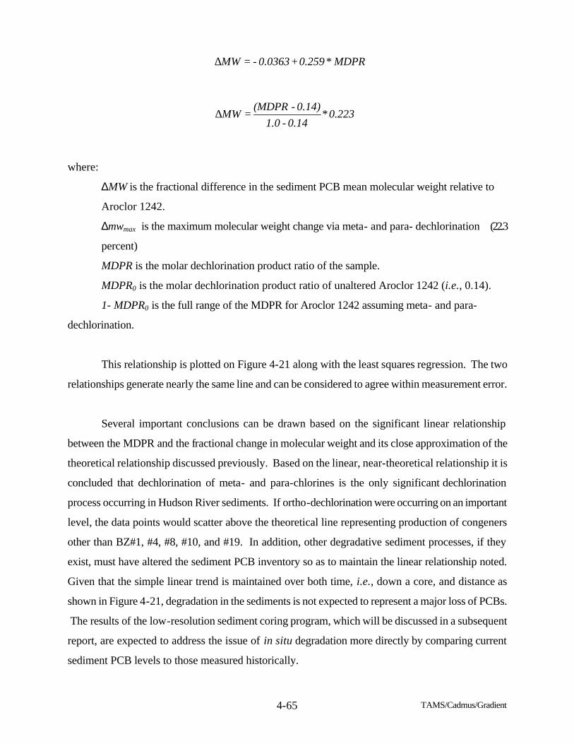
TAMS/Cadmus/Gradient 4-65
where:
∆MW is the fractional difference in the sediment PCB mean molecular weight relative to
Aroclor 1242.
∆mwmax is the maximum molecular weight change via meta- and para- dechlorination (22.3
percent)
MDPR is the molar dechlorination product ratio of the sample.
MDPR0 is the molar dechlorination product ratio of unaltered Aroclor 1242 (i.e., 0.14).
1- MDPR0 is the full range of the MDPR for Aroclor 1242 assuming meta- and para-
dechlorination.
This relationship is plotted on Figure 4-21 along with the least squares regression. The two
relationships generate nearly the same line and can be considered to agree within measurement error.
Several important conclusions can be drawn based on the significant linear relationship
between the MDPR and the fractional change in molecular weight and its close approximation of the
theoretical relationship discussed previously. Based on the linear, near-theoretical relationship it is
concluded that dechlorination of meta- and para-chlorines is the only significant dechlorination
process occurring in Hudson River sediments. If ortho-dechlorination were occurring on an important
level, the data points would scatter above the theoretical line representing production of congeners
other than BZ#1, #4, #8, #10, and #19. In addition, other degradative sediment processes, if they
exist, must have altered the sediment PCB inventory so as to maintain the linear relationship noted.
Given that the simple linear trend is maintained over both time, i.e., down a core, and distance as
shown in Figure 4-21, degradation in the sediments is not expected to represent a major loss of PCBs.
The results of the low-resolution sediment coring program, which will be discussed in a subsequent
report, are expected to address the issue of in situ degradation more directly by comparing current
sediment PCB levels to those measured historically.
MDPR * 0.259 + 0.0363 - = MW∆
0.223 * 0.14 - 1.0
0.14) - (MDPR = MW∆
TAMS/Cadmus/Gradient 4-66
The absence of ortho-dechlorination is consistent with the findings of several Hudson River
investigations (Abramowicz et al., 1993; Quensen et al., 1990; J. Brown et al. 1987; and Rhee et al.,
1993b). However, the Phase 2 investigation represents the most extensive coverage of Hudson River
sediments and confirms the absence of ortho-dechlorination over 110 miles of the river. The
suggestion that dechlorination is the only significant process affecting sediment PCB levels represents
an important concept. The fact that meta- and para-dechlorination can only decrease the PCB mass by
a maximum of 26 percent implies that sediment PCB inventories sequestered over the previous 40
years (1954 to 1994) will remain in place unless subject to scour, extensive purging by porewater, or
remediation. Although some authors have demonstrated degradative PCB losses from the sediments
(e.g., Rhee et al., 1993b), these losses do not appear significant for the mix of PCB congeners present
in the Hudson. This issue will also be examined in the analysis of the low-resolution sediment coring
program.
Also shown in Figure 4-21 are the theoretical results for seven unaltered Aroclor mixtures
(Aroclors 1221, 1232, 1016, 1242, 1248, 1254, and 1260). The Upper and Lower Hudson sediment
data clearly define a line which intersects with the Aroclor 1242 conditions, strongly suggesting that
this mixture represented the dominant Aroclor form sequestered in the sediments of the main-stem
Hudson. This is consistent with the results discussed in Chapter 3 which show the combined
Thompson Island Dam load to dominate the entire freshwater Hudson PCB loading, and with the fact
that the GE releases consisted principally of Aroclor 1242. The similarities between Aroclor 1242
and Aroclor 1016 by this measure are sufficient that the presence of Aroclor 1016 in the sediments
cannot be ruled out. In any event, the presence of Aroclor 1016 is still consistent with a load derived
from the Upper Hudson.
It is interesting to note that the Lower Hudson MDPR and ∆MW values shown on Figure 4-21
generally fall just to the left of Aroclor 1242 but along the same linear relationship as the Upper
Hudson results. If other Aroclors were added to the Upper Hudson mixture, the data should cluster
along lines connecting the Aroclor 1242 conditions with those of the added mixture. The data
distribution indicates that while the addition of heavier Aroclors may be partially responsible for the
distribution of the Lower Hudson results, this is not sufficient. Instead, the data suggest that some
alteration or degradation of the original PCB mixture has occurred. The alteration appears to be
relatively minor, resulting in a change in molecular weight generally less than 6 percent (see Figure 4-
TAMS/Cadmus/Gradient 4-67
20). Although not evident in this figure, the values for the MDPR and ∆MW are not temporally
dependent, suggesting that this degradation is occurring during transport or just after deposition. The
lack of variation with time again suggests that in situ degradation is not an important factor for the
PCBs in the sediments of this region of the Hudson. Evidence for the lack of time dependence will be
given later in this section.
One last important feature is evident on Figure 4-21. The results for essentially all background
and tributary sediments (virtually all of which have an MDPR of 0.0) lie well away from the Upper
and Lower Hudson regression line and the theoretical dechlorination line. This indicates that the PCB
mixtures carried by the associated tributaries are significantly different from those of the main-stem
Hudson. In general, these tributaries tend to contain more-chlorinated congener mixtures, probably
derived from heavier Aroclors. In addition, it indicates that the tributary loads cannot be at all
significant, since the addition of substantial non-Aroclor 1242 loads would destroy the linear
relationship between the MDPR and the ∆MW. These results, along with findings present in Chapter
3, suggest that the only significant source of Aroclor 1242 (and PCBs in general) to the freshwater
Hudson is the GE facilities. The tributaries contain at most only trace levels of this Aroclor mixture
and thus cannot be significant contributors to the Hudson River PCB inventory.
Given that Aroclor 1242 is the likely primary original PCB congener mixture for the entire
freshwater Hudson, it is then appropriate to calculate the actual mass loss documented by the change in
molecular weight. This calculation was done for all the Upper Hudson sediment samples and is
summarized in Table 4-11. Note the low degree of actual mass loss for the Upper Hudson sediments.
The mean mass loss is about 8 percent. The maximum mass loss for these sediments is 25 percent.
The mass loss calculation was not done for the Lower Hudson sediments since so many lie below the
Aroclor 1242 value, indicative of weathering of the PCB mixture prior to deposition as discussed
above. The small average mass for the Upper Hudson sediments indicates that the sediment inventory
has been left largely intact by the dechlorination process.
TAMS/Cadmus/Gradient 4-68
Correlation of the Degree of Dechlorination with the Total PCB Concentration
As part of the Phase 2 data analysis, an attempt was made to understand the factors governing
the extent of dechlorination. Several authors have suggested that the extent of dechlorination is related
to the initial concentration of PCBs in the sediments, e.g., Quensen et al. (1988), Rhee et al. (1993a),
and J. Brown et al. (1987). These authors found that, in general, the higher the initial concentration,
the greater the extent of dechlorination. The results of the Phase 2 sampling program are consistent
with these findings as discussed below.
Figure 4-22 demonstrates the relationship between the molar dechlorination ratio and the total
PCB concentration for all post-1954 high-resolution sediment core samples collected between RM 88
and RM 203, representing freshwater sediments only. To avoid the uncertainty when results are close
to the detection limits, this plot only uses data from sediment-core samples containing PCB levels of at
least 100 µg/kg (ppb) of total PCBs, i.e., the sum of the 126 measured congeners was equal to or
greater than 100 µg/kg. Also as mentioned above, only samples which had measurable levels of 137Cs
were used. The figure shows that the data fall into two different regimes. Results from the main-stem
Hudson form a linear relationship between the MDPR and the log of the Total PCB concentration.
(Note that the Total PCB concentration scale on the figure is logarithmic.) The second regime consists
largely of the background and tributary results and shows no relationship with PCB concentration.
This is consistent with the results shown in Figure 4-21 which show the background and tributary
results to be quite different from those of the main-stem Hudson based on the two measures used.
The results depicted in Figure 4-22 lead to several important conclusions concerning
dechlorination. Primarily, the figure shows that the degree of dechlorination is correlated with the
Total PCB mass content of the sample at time of collection, and by inference, at the time of deposition.
Second, the figure suggests that this relationship is consistent throughout the Hudson downstream of the
GE facilities. The degree of dechlorination scatters fairly consistently about the line and yields a
relatively good r2 value of 0.75 out of a possible 1.0. The line was fit to all Hudson River mainstream
sediment results. As illustrated by the figure, this relationship applies over four orders of magnitude
of PCB concentrations. The scatter is such that the value of the MDPR is not consistently above the
assumed initial value of 0.14 based on Aroclor 1242 until the Total PCB concentration is greater than
TAMS/Cadmus/Gradient 4-69
about 30,000 µg/kg (30 ppm). This concentration is the point at which the lower 95 percent confidence
interval about the data reaches the MDPR value of 0.14. The distribution of the data strongly suggests
that virtually all samples with PCB concentrations greater than 30 ppm are measurably altered with
respect to Aroclor 1242.
A third conclusion can be drawn by comparing the results for Upper and freshwater Lower
Hudson core sites shown in Figure 4-22. It is evident that average PCB concentrations in the Upper
Hudson i.e., RM 198 through RM 157, are substantially higher than those in the freshwater portion of
the Lower Hudson, i.e., RM 153 through RM 88. PCB concentrations in sediments from the major
tributaries, i.e. the Mohawk and Hoosic Rivers and the Batten Kill, are among the lowest
concentrations. In fact, few main stem Hudson samples fall below 800 µg/kg (0.8 ppm) while the
majority of the tributary samples fall well below this value, again emphasizing the magnitude of the
GE releases relative to all other sources. This figure also illustrates that, although sediment samples
collected from the Upper Hudson generally show significantly more dechlorination relative to
locations downstream, this occurrence is not related to location per se but rather to the amount of
PCBs in the sediments regardless of location. Levels of dechlorination equivalent to those of the
Lower Hudson can be seen in sediments of the Upper Hudson when concentrations are comparable. In
fact, a broad range of sediment dechlorination ratios can be found within a single core, as shown in
Figures 4-23 and 4-24.
Figure 4-23 shows the relationship between the MDPR and PCB concentration in Core 18
collected at RM 185.5, as well as how the ratio varies from core top to bottom. Similar degrees of
dechlorination are found at both ends of the core with the peak dechlorination occurring at mid-depth,
coincident with the maximum Total PCB concentration. Figure 4-24 shows the same information and a
similar relationship for Core 19 collected at RM 188.6.
The fractional change in molecular weight was also correlated with the Total PCB
concentration, as would be expected. Figure 4-25 shows the relationship between the two variables.
Again the degree of dechlorination varies linearly with the log of the Total PCB concentration. A
somewhat more variable but still significant correlation is shown (r2 = 0.73). On this figure the
background and tributary samples are again clearly separate from those of the main stem Hudson, as
noted in earlier figures. The regression line represents a fit to main-stem Hudson River freshwater
TAMS/Cadmus/Gradient 4-70
sediment samples only. Figure 4-26 represents an expanded-scale representation of the main-stem
Hudson data. At this scale it is apparent that the change in molecular weight steadily increases with
increasing values of the log of the PCB concentration. Like the data shown in Figure 4-22 for the
MDPR, the variability of the fractional change in molecular weight (∆MW) is such that the ∆MW is
not consistently greater than zero in samples with PCB concentrations less than 30,000 µg/kg (30 ppm).
Given the correspondence of ∆MW and mass loss, it is important to note that sediments with
PCB concentrations less than the 30,000 µg/kg threshold, on average, experienced little, if any, mass
loss via dechlorination. Mass loss greater than 10 percent is generally restricted to sediments of
30,000 µg/kg or higher, which in turn are still subject to the maximum loss of 26 percent.
Both the MDPR and the ∆MW correlate well with the log of the Total PCB concentration.
Based on these correlations, location and sediment age should not be important variables influencing
the degree of dechlorination. As shown in Figures 4-22 and 4-26, location, i.e., Upper Hudson vs.
Lower Hudson, is not important to the degree of dechlorination. The lack of time dependence can also
be inferred from these figures with some knowledge of the PCB release history. However, given the
importance of this issue, this was addressed directly.
Figure 4-27a shows the relationship between the MDPR and depth for all high-resolution
cores. Although many of these cores could not be dated as described in Subsection 3.3.1, depth can
serve as a rough surrogate for age in sediment cores, since deeper sediments can be assumed to be
older than shallower ones. The data in Figure 4-27a represent the same samples as shown in Figures
4-21, 4-22, 4-25, and 4-26. The data appear widely scattered and illustrate the lack of correlation
between depth and dechlorination ratio, and by inference, the absence of a strong relationship between
time and the dechlorination ratio. The maximum MDPR within individual cores occurs at mid-depth
levels, at about 15 to 40 cm. This depth generally coincides with the occurrence of the Total PCB
concentration maximum as shown in Figure 4-27b.
The absence of a correlation with time can be seen more clearly in a subset of the samples
represented above. Using only dated sediment cores from the freshwater main stem Hudson, the
degree of dechlorination as measured by the ∆MW is plotted in a histogram as a function of time of
deposition (see Figure 4-28a). The data are grouped into approximately ten year intervals beginning
TAMS/Cadmus/Gradient 4-71
in 1954. Evident in the diagram is the clustering of the values around a ∆MW value of 0. More
important for this discussion, however, is the fact that a wide range of mass loss (i.e., ∆MW) can be
seen for any time period, indicating the lack of time dependence for this process. The samples with
the greatest degree of dechlorination are from the period 1965 to 1974. However, this period also
contains samples with essentially no measurable dechlorination. Similar ranges can be seen for the
periods 1955 to 1964 and 1975 to 1984. Only the most recent period presented, 1985 to 1992, has a
lesser range. However, its results are still consistent with those of the previous time periods. The
limitation here is simply that water column PCB loads during this most recent period were less than
those of the earlier periods, resulting in lower sediment PCB levels. (Historical water column
transport is discussed in detail in Section 3.3.)
These same data are represented in Figure 4-28b. In this diagram the ∆MW values are plotted
against the total PCB concentration as was done in Figure 4-26. The data are color-coded on the same
basis as Figure 4-28a with different symbols to indicate river area. This diagram shows how the level
of dechlorination in any time period varies as a function of concentration as was noted for the entire
data set.
The evidence presented in Figures 4-27, 4-28a and 4-28b clearly documents the absence of
any long-term temporal dependence of the degree of dechlorination. The conclusion that the degree of
dechlorination is not dependent upon the age of the sediments implies that the sediment dechlorination
process occurs relatively rapidly, within several years of deposition. The ultimate level of
dechlorination is determined by the PCB concentration originally deposited. After the degree of
dechlorination commensurate with the sediment PCB concentration is attained, the dechlorination
process appears to stop and the PCBs simply remain in the sediment. This suggests that the long-term
fate of PCBs is controlled only by scour, burial or dissolution; i.e., that in situ destruction by
dechlorination will not eliminate the Hudson's PCB inventory. Indeed, in sediments with PCB levels
at 30,000 µg/kg or less, dechlorination does not appear to be significant at all. This conclusion is
supported by the analysis of the dated sediment congener patterns discussed in Subsection 3.3.3,
which shows little evidence of alteration for the period 1975 to 1992.
It is important to reiterate here that samples with the highest degree of dechlorination have only
lost about 20 percent of their original PCB mass to this process even though many of the original
TAMS/Cadmus/Gradient 4-72
molecules have been affected by dechlorination. Given the consistent relationship between the
fractional change in the molecular weight and the MDPR, it appears unlikely that other processes are
substantially altering the sediment PCB inventory. Thus it is likely that the majority of Hudson River
sediment PCB levels are within 20 percent of their original concentration as deposited.
Up to this point, this discussion has dealt solely with freshwater sediments and dechlorination.
As part of the Phase 2 investigation, several cores were collected from the brackish portion of the
Hudson, i.e., below RM 60. These cores show no substantive dechlorination, as evidenced by the
absence of elevated levels of the four final dechlorination congeners discussed above. This is
consistent with the work by Abramowicz et al. (1993) who found that sea salt inhibited dechlorination
in a laboratory study using freshwater Hudson River sediments. Although this study used microbes
which originated from a freshwater environment, and thus may not be strongly adapted to saline
environments, dechlorinating microorganisms do not appear to be present below RM 60. An example
of the largely unaltered profiles from the brackish portion of the Hudson can be found in Subsection
3.3.3.
4.4 Implications of the PCB Fate in the Sediments for Water Column Transport
In the three previous sections of this chapter, the discussion has centered on assessing the
likely current inventory of PCBs in the sediments of the Upper Hudson River. As part of this
discussion, evidence was presented to estimate the extent of dechlorination of PCBs within the
sediments. Using the same basis of measurement, specifically the molar dechlorination product ratio
(MDPR), this section will examine how these dechlorinated PCBs impact the water column. In
addition, the characteristics of the sediments responsible for the water column impact will be
examined. This discussion will provide a basis for further examination of the nature of sediment-water
interactions in subsequent Phase 2 reports.
Given the strict adherence of the MDPR and fractional change in molecular weight (∆MW) to
a linear relationship for essentially all sediments of the freshwater Hudson, the water column samples
were examined in a similar manner. As the first step in this analysis, the MDPR and ∆MW for water
column Stations 4 and 5, representing the Rogers Island and Thompson Island Dam locations
respectively, were examined. These results are shown graphically in Figure 4-29. As can be seen in
TAMS/Cadmus/Gradient 4-73
this figure, both stations obey the same linear relationship established in the sediment analysis. The
results plotted here represent whole-water samples for each location for each sampling event, i.e.,
each point represents the sum of the PCB results for the dissolved and suspended matter samples
collected at each station for a given event. Both the transect and the flow-averaged results are
represented in the figure. As can be seen, the results for the two stations are generally well separated,
with the Rogers Island samples centered around Aroclor 1242 and the Thompson Island Dam samples
at the high end of the line, with MDPR values around 0.6 to 0.75.
The implications of Figure 4-29 are consistent with the conclusions of Chapter 3. Specifically,
upstream of Rogers Island, a PCB load which is similar to Aroclor 1242 in its congener content enters
the river. As the river travels through the Thompson Island Pool, the nature of the water column
congeners mixture changes markedly. The mixture leaving the Thompson Island Pool is distinctly
lighter (lower molecular weight) with a much larger proportion of mono- and di-chlorinated
homologues. The data as plotted suggest a two end-member mixing system as the operating mechanism
for this portion of the Hudson. A two-member mixing system is one in which two sources are mixed
together in simple proportions. All samples collected from such a system can be described as x
percent of end member (source) 1 and (1-x) percent of end member 2. The two end members in this
instance are the Aroclor 1242-like source above Rogers Island and the partly dechlorinated PCBs
from the sediments of the Thompson Island Pool. There are two exceptions to this finding, the first of
which is the Rogers Island sample with a MDPR of about 0.78. This sample was collected during
Transect 5 and is believed to be contaminated with Thompson Island Pool sediment which was
disturbed during sample collection. (The sample had an extremely high suspended solids concentration
for the flow conditions at the time of sampling and matched the typical sediment congener pattern.) The
second exception is the value which lies well away from the line. This sample was collected during
Transect 1 and is unlike any other sample collected during the Phase 2 investigation. The Thompson
Island Dam samples with low MDPR values were collected during periods of high spring flow when
transit times through the Pool were short and the load originating above Rogers Island was quite large.
In these instances, the impact of the Thompson Island Pool sediments appears to be smaller but still
consistent with a two end member mixing system.
An important conclusion to be drawn from Figure 4-29 is the apparent similarity between the
sediment characteristics and those of the water column. As discussed in Chapter 3, the congener
TAMS/Cadmus/Gradient 4-74
distribution of the dissolved and suspended matter fractions are quite different due in part to the
variation of PCB congener affinity for sediments relative to water. Yet, when these two components of
the water column PCBs (i.e., the dissolved fraction and the suspended-matter fraction) are viewed as
a whole, they provide a consistent picture of a sediment-like source originating in the Thompson
Island Pool. The fact that the congener distribution of the dissolved and suspended matter fractions are
so different at the Thompson Island Dam despite the proximity to the likely source, i.e., the Thompson
Island Pool sediments, suggests that equilibrium between the dissolved and suspended matter PCB
fractions is rapidly attained upon the addition of PCBs to the water column.
The consideration of the whole water homologue pattern leads to a second important issue. In
previous discussions, the load at Thompson Island Dam has been described as the sum of all upstream
loads, including a net Thompson Island Pool load gain. Alternatively, it was suggested that the load at
the Thompson Island Dam was generated within the Pool, independent of the upstream loads under
low-flow conditions. In the latter instance, the source to the water column would resemble the
sediments whose MDPR and molecular weight match the red circles on Figure 4-29. Thus, the source
material for the Thompson Island Dam load, assuming upstream loads are not passed through, are
those sediments with an MDPR of 0.55 to 0.75 and a molecular weight 10 to 15 percent lower than
Aroclor 1242.
However, if the Thompson Island Pool acts as a conduit for the upstream loads then the
Thompson Island Pool source must be mixed with the incoming load from Rogers Island. In order to
obtain the properties of the Thompson Island Dam load, the source would have to have a greater
degree of alteration. Figure 4-30 shows the properties of the Thompson Island Pool source term
assuming that the Rogers Island mixture is transferred conservatively through the Pool. Note that the
source properties are still defined by the sediment regression line; but the source material has an even
higher MDPR and lower molecular weight. Thus the source material resembles sediments which have
undergone an even greater degree of dechlorination. Given the requirement that extensive
dechlorination only occurs at high PCB concentrations, it is likely that this source is highly altered,
highly concentrated PCB-bearing sediment. This raises a significant question: How likely is it that
material of this type is available to interact with the water column? Before answering this question a
second issue should be addressed. Not all Rogers Island-Thompson Island Dam sample pairs could be
used to calculate this net source term properties. Several pairs showed significant losses for several
TAMS/Cadmus/Gradient 4-75
congeners, thus generating theoretically impossible source mixtures since this calculation assumes that
the sample mixture is achieved by simple addition (congener loss by addition of two mixtures is not
allowed). These instances constitute strong evidence for the suggestion that some, if not all, of the
upstream load is sequestered in the Thompson Island Pool under low-flow conditions and that the
Thompson Island Pool is responsible for much more than the simple net load gain as noted at the
Thompson Island Dam.
The remaining (downstream) water column samples were also examined in this manner. These
results are shown in Figure 4-31. The water column data points have been color coded to
denote the season of collection. It can be seen in this figure that the water column samples collected at
each of the stations tend to follow the same linear relationship between ∆MW and MDPR as that for
the sediments. However, these points generally fall between the Rogers Island and the Thompson
Island Dam samples, indicating that the water column fraction of the dechlorination product congeners
(BZ#1, 4, 8, 10 and 19) decreases as the water moves downstream. This phenomenon is more clearly
evident when the water column data are viewed on a single event basis. Figure 4-32 shows a
comparison between the MDPR and the ∆MW for the six water column transects. For each transect, a
line traces the path of the water column PCB characteristics. In five of the six events, the Thompson
Island Pool (Station 5) represents the highest point on the graph, with subsequent downstream points
moving downward along the sediment regression line. Note that for Transects 1, 4, and 6, station data
for samples collected in the freshwater Lower Hudson are also shown (Stations 14 to 17).
In Transects 1 and 3, values for the Upper Hudson stations downstream of the TI Dam remain
close to the TI Dam value (station 5). The exception here being the Transect 3 Station 8 value
(Waterford) which reflects the Hoosic River-induced scour event. These values are consistent with
the discussions in Section 3.2 whereby little change in the PCB homologue pattern and load occur
between TI Dam and Waterford.
For Transect 4, which corresponds to the spring runoff event, there is little variation
downstream of Rogers Island. This is believed to be due to both the high water flow and the large
upstream PCB flux which occurred at this time, possibly serving to overwhelm any input from
downstream sediments.
TAMS/Cadmus/Gradient 4-76
Under summer conditions, the change in congener content represents a shift toward less
dechlorinated mixture downstream of the Thompson Island Dam. Although the exact reason for this
change is unclear, the consistency of the Thompson Island Dam station samples and the gradual
variation of the samples collected at downstream stations relative to the Thompson Island Dam station
samples suggest either a sediment-related exchange (i.e., resuspension, settling and/or porewater
exchange) or biological activity as likely explanations. This is consistent with the discussions in
Section 3.2.
Transect 2 does not conform to these conventions since it shows substantial variation in ∆MW
downstream of the TI Dam during winter conditions. The reason for this is not known but is believed
to be related to analytical problems associated with Transect 2 samples.
For both winter and summer conditions, stations in the Lower Hudson generally move toward
lower MDPR and ∆MW values. This is probably due to greater sediment-water interaction in this
region, driven by total energy and enhanced by the slower net downstream movement of the tidal
Lower Hudson.
Focusing again on the variation in MDPR and ∆MW under summer conditions, the sediment-
related PCB exchange relationship developed in Section 4.3 becomes important, i.e., the degree of
PCB dechlorination varies with the log of the PCB concentration; the higher the concentration, the
greater the degree of meta- and para-dechlorination. As noted in Chapter 3, Subsection 3.3.3, the
concentration of PCBs in the sediments steadily decreases with distance downstream away from the
Thompson Island Dam. Taken together, these observations suggest that the degree of PCB
dechlorination in the sediments should generally decrease downstream of the Thompson Island Dam.
This conclusion is supported by Figure 4-33 which shows the decline in total PCB concentration and
MDPR for surficial high resolution core sediment samples with river mile beginning at RM 195.
Although the samples are biased toward fine grained sediments, they should still reflect the overall
trend in the Hudson River.
Given the decrease in PCB dechlorination with distance downstream of the Thompson Island
Dam, the degree of PCB dechlorination measured in the water column is likely to be the result of the
primary input from the Thompson Island Pool (see Sections 3.4 and 3.6 for a summary discussion of
TAMS/Cadmus/Gradient 4-77
the magnitude of this source) and the degree of water-sediment interaction downstream of the
Thompson Island Dam. The exchange of PCBs between the water column and the sediments is a
process which is dependent upon sediment resuspension and settling, pore water exchange, and
diffusion. In addition, processes within the water column may alter the mixture as well. The degree to
which each of the processes is important will depend upon river flow, groundwater recharge, and
temperature, at minimum. In light of the strong linear relationship among water column stations
demonstrated in Figure 4-31, whatever processes responsible for the exchange must effectively act as
a simple mixing mechanism between less chlorinated (Thompson Island Pool-like sediments) and
more chlorinated (Aroclor 1242-like sediments) PCB congener mixtures. It is likely that the
importance of any single process will vary both with time and location. The modeling program to be
conducted in Phase 2 will deal with these processes directly. However, it is still useful here to
examine the data further to suggest a likely scenario for the exchange process.
It is important to note here that the mechanism for PCB exchange between the water column
and sediments affects the type of PCB mixture which enters the water. In the case of sediment
resuspension, the homologue pattern, MDPR and ∆MW of the PCBs added to the water column will
probably be similar if not identical to those of the resuspended sediments. Conversely, PCBs added to
water column via porewater must undergo an alteration in the homologue pattern, MDPR and ∆MW
consistent with sediment-porewater equilibrium. This is discussed in Sections 3.1 and 3.2. In
particular, Figures 3-36 and 3-37 show a possible sediment to porewater homologue pattern alteration
based on the Phase 2, two phase equilibria constants developed in Section 3.1. Based on these
figures, the equilibration process between sediment and porewater apparently serves to create a
porewater PCB mixture which is less chlorinated than the sediment PCB mixture from which it was
derived.
As discussed in Chapter 3, the PCB load entering the Thompson Island Pool is similar in
nature to unaltered Aroclor 1242. Figure 4-34 shows the examples of the Rogers Island PCB mixture
compared with Aroclor 1242 on a homologue basis. Although there are some differences when
viewed on an individual congener basis, the resemblance between the mixtures is strong. In light of all
the recent revelations concerning the GE Hudson Falls facility, it is highly likely that this load is
principally derived from unaltered PCB product leaking from the facility. Once below Rogers Island,
however, it is clear that the water column mixture is no longer primarily driven by this source. This is
TAMS/Cadmus/Gradient 4-78
particularly evident in the three diagrams which compare the Thompson Island Dam water column
samples with Aroclor 1242 as well as with three different sediment mixtures. The sediment mixtures
shown in Figure 4-34 for the TI Pool and other locations represent samples collected from cores. At
the specified location (TI Pool, RM 177.8, etc.), these were selected to match the water column
pattern based on their MDPR value. As noted in Section 4.3, the MDPR and homologue pattern vary
with the total PCB concentration. Hence, several different sediment samples were used to correlate TI
Pool water column conditions.
In each of the TI Dam diagrams, the water column mixture is distinctly sediment-like and bears
little resemblance to Aroclor 1242. These three diagrams also suggest that the mixture of the sediment
driving the PCB load at the Thompson Island Dam varies, ranging in the degree of dechlorination, and
by inference, concentration. It should be noted that although there is good agreement on a homologue
basis, there are some differences which become evident only when viewed on a congener basis.
These differences may be attributed to several considerations, including sediment PCB pattern
variation as well as processes such as gas exchange or biological degradation which may affect the
PCB mixture once it enters the water column.
It is evident from these diagrams that the sediments of the Thompson Island Pool closely
resemble the load at the Thompson Island Dam and that PCBs in these sediments are altered relative to
Aroclor 1242. As noted previously in the discussion of Figure 4-32, downstream PCB mixtures under
summer conditions are less altered and more Aroclor 1242-like. However, as shown in Figure 4-34
for samples collected at Stillwater, Waterford, and Highland, this shift is likely the result of additional
mixing between the water column and the less altered sediments downstream or in situ processes.
The shift is not the result of additional fresh Aroclor 1242 being added to the water column. In the
three water column samples collected at Waterford, the similarity to the sediment is clearly better than
the match to Aroclor 1242. In Transect 1, the pattern closely resembles sediment from the TI Pool,
consistent with the conservative PCB transport and lack of downstream variation seen in this transect.
Of particular note is the Transect 3 sample collected at Waterford. During this transect, scouring of
Hudson River sediments occurred due to the 100-year flow conditions on the Mohawk River. As can
be seen in Figure 4-32, this sample appears similar to Aroclor 1242 in terms of its BZ#1, 4, 8, 10, and
19 (dechlorination products) content. However, as shown in Figure 4-34, the homologue pattern is
more similar to the moderately altered sediments in this area of the Hudson River than to Aroclor
TAMS/Cadmus/Gradient 4-79
1242. Similarly, the Stillwater sample shown in Figure 4-34 which was not affected by the scour
event is more similar to Upper Hudson sediments than to fresh Aroclor 1242. Again these results are
consistent with the TI Dam pattern seen throughout this transect above Waterford. Thus, the change in
MDPR and ∆MW of the water column PCB inventory at the TI Dam and points downstream appears to
be the result of sediment-water exchange and not the result of any new additions of fresh Aroclor
1242. The absence of fresh Aroclor 1242 in the water column is consistent with the conclusions of
Chapter 3 concerning total PCB loading patterns, i.e., that little additional external PCB loading
occurs downstream of the Thompson Island Dam.
The close agreement between sediment and water homologue patterns suggests a strong link
between the two matrices. However, processes such as aerobic degradation are also undoubtedly
involved as well. In fact, the homologue patterns seen in the sediments and water column in the area
around Waterford indicate the likelihood of degradation of the upstream load. This process is
suggested by the patterns seen in the Waterford sample results for Transects 3 and 6. In Transect 3, the
sediments scoured from the river bottoms are not extensively dechlorinated but do not resemble
Aroclor 1242 either. These sediments and probably most of the sediments represented by the samples
with MDPR values less than 0.14 appear to have undergone a degradation process which has
selectively removed some congeners, yielding the pattern seen in the scoured sediment. Similarly in
Transect 6, the water column inventory steadily changes from the TI Dam to Waterford, suggesting
either a water column-based loss of lighter congeners or sediment-water exchange or both in order to
modify the water column PCB homologue pattern. Regardless of the nature of the alteration, however,
the strict adherence of all sediment and water samples to a linear relationship, as shown in Figures 4-
29 and 4-31, suggests that the process cannot extensively modify the total PCB inventory; extensive
modification to the water column PCB inventory by aerobic processes would probably alter the linear
relationship between the MDPR and ∆MW. This suggests that the dechlorination process, which is
limited to a theoretical maximum mass loss of 26 percent, is the principal means of PCB mass
reduction in the Hudson River.
Figure 4-34 and the water column PCB loading figures presented in Chapter 3, demonstrate the
importance of the Thompson Island Pool sediments in generating a significant water column PCB load.
In Figure 4-34 as well as in Figures 3-38 and 3-40, the Thompson Island Pool appears to be the
principal source to the water column during winter and spring with little downstream sediment-water
TAMS/Cadmus/Gradient 4-80
exchange. This is suggested by the preservation of the Thompson Island Dam homologue pattern
between the Thompson Island Dam and Waterford. During late spring and summer, downstream
sediment-water exchange becomes more important, as is evident in the change in homologue patterns.
In all instances, however, the fresh unaltered Aroclor 1242 pattern is absent, suggesting a minimal
importance of the GE Hudson Falls source during most of the year. Only during spring runoff, when
release from the GE Hudson Falls source is large, is the pattern of the upstream load present
throughout the Upper Hudson.
As is indicated by the water column sample collected at Highland and presented in Figure 4-
34, in the Lower Hudson, PCB homologue patterns in the water column and sediment are both similar
to unaltered Aroclor 1242. As noted in Figure 4-19, 20 and 21, the PCB mixtures of the Lower
Hudson tend to have lower MDPR and ∆MW values than that of fresh Aroclor 1242. In addition,
because this pattern is not transported directly from the Upper Hudson during much of the year (as seen
in the water column pattern) and, on a total load basis, little additional external PCB loading is
incurred below the Thompson Island Dam, it appears that the close agreement between water and
sediment is again the result of sediment-water exchange and does not indicate fresh additions of
Aroclor 1242.
The discussions above clearly note the close correlation between the homologue pattern of the
water column and the sediments. For the sediments to directly drive the water column load, their PCB
mixtures must be directly added to the water column without alteration. The processes of
resuspension and settling would serve to accomplish this. These processes could also serve to
remove some or all of an upstream load as PCBs sorbed to settling particles. Given sufficiently high
rates of gross settling and resuspension in the TI Pool, the upstream load can easily be replaced and
the total load increased with PCBs from the Pool. However, as noted in Section 3.2, porewater is
also a viable means for PCB transfer from the sediments. To explore this transfer, water column
homologue patterns were compared with theoretical porewater mixtures derived from two phase
partition coefficients. These theoretical mixtures were synthesized using congener-specific partition
coefficients and the homologue pattern present in various Hudson River sediments as described in
Section 3.2. Figure 4-35 presents a comparison between several TI Dam and Waterford samples and
high resolution sediments core samples found in the general vicinity. These diagrams show that in
some instances the porewater represents a good match to the water column pattern. While this does not
TAMS/Cadmus/Gradient 4-81
constitute a proof, it suggests that porewater may be an important exchange mechanism, particularly in
summer when homologue patterns distinctly change downstream of the Thompson Island Dam. Also
shown in Figure 4-35 is a Thompson Island Pool sample from Transect 3. In this instance, the
sediments are slightly better matched suggesting other transport mechanisms.
There is an important distinction to be made here concerning the nature of the TI Pool PCB
source. If sediments are suspended via resuspension, then the sediments must be extensively
dechlorinated so as to match the patterns seen in the water column. Alternatively, if the load from the
TI Pool occurs via porewater exchange, then the sediment source must be less dechlorinated than the
load they produce since the equilibration process preferentially dissolves less chlorinated congeners.
The porewater patterns shown in Figure 4-35 were generated from sediments with relatively low
concentration and commensurately low levels of dechlorination.
These observations suggest the following scenario for water column PCB loads. During cool,
low-flow conditions, the Upper Hudson water column conditions are controlled by the sediments of
the Thompson Island Pool via either resuspension or porewater exchange and the congener pattern is
preserved throughout the Upper Hudson. During warm, low flow conditions, the Thompson Island
Pool sediments are still locally important but, upon transport downstream, sediment-water exchange
such as porewater transport and/or possibly in situ water column processes modify the water column
congener mixture yielding a less dechlorinated result. Only during spring runoff is the homologue
pattern observed at Rogers Island evident at downstream locations. In terms of total PCB transport as
presented in Chapter 3, the Rogers Island and Thompson Island Pool sources appear roughly equal
when examined over the period 1993 to the present. In terms of temporal importance, the sediments of
the Upper Hudson, particularly those of the Thompson Island Pool, are clearly more important. During
the post-1993 period, the TI Pool is clearly the most important source even on an annual basis.
Having established the importance of the Upper Hudson sediments, particularly the Thompson
Island Pool sediments, to water column PCB loads, it is useful to further characterize the responsible
sediments. If porewater exchange is the primary driver then little can be said other than that the
sediments responsible must be relatively unaltered and therefore at relatively low concentrations.
However, if resuspension is responsible for the load, the responsible sediments can be more
accurately described.
TAMS/Cadmus/Gradient 4-82
As noted in Figure 4-29, the MDPR for the Thompson Island Dam water column samples is in
the range of 0.55 to 0.75. This is shown again in the first diagram of Figure 4-36. If it is assumed that
the water column pattern is directly obtained from the sediments, then the sediments responsible for
this load must be in the range of 120,000 to 700,000 µg/kg as shown in the second diagram in Figure 4-
36. This second diagram is based on Figure 4-26. Note that this represents a lower bound on the
concentration range since it assumes that the entire pattern is generated by the sediment and that none
of the upstream load is transported through the Thompson Island Pool, i.e., all of the Rogers Island
loading is trapped within the Thompson Island Pool. If this is not the case, then the sediments causing
the Thompson Island Dam pattern must be even more altered and therefore more contaminated in order
to shift the water column homologue pattern.
Given the minimum concentration range for the sediment, it is then possible to estimate the
likely minimum sediment age, i.e., the time of deposition for these sediments. Using the high resolution
core collected at RM 188.5 near the Thompson Island Dam (Core 19) as a record of the PCB
concentration in accumulating sediments, the data suggest that the sediments are at least 10 years old,
since 1983 was the last time that sediments in the range of 120,000 µg/kg or greater were deposited.
This is shown in the last diagram of Figure 4-36. Given the large mass of sediments with even higher
PCB concentrations deposited prior to 1983, it is likely that the responsible sediments are even older.
It should be noted that the recent releases (September 1991 - June 1993) from the GE Hudson
Falls area which occurred during the time of the high resolution core collection may have resulted in
sediments with sufficiently high concentration so as to support a similar level of dechlorination.
While no evidence for these sediments were found in the high resolution cores, core collection
performed subsequent to the Phase 2 period (Chillrud et al., 1996) suggest that some higher sediment
concentrations did result, at least in the Lower Hudson. However, in order to be solely responsible
for the TI Pool source via resuspension, these freshly deposited sediments would have to be quickly
buried and dechlorinated. It is more likely that these materials, in combination with the existing TI
Pool sediment inventory, are responsible for the TI Pool source, i.e., the source results from a
combination of altered sediment and freshly deposited sediment whose net result is a mixture whose
properties closely resemble those of 1984 sediment.
TAMS/Cadmus/Gradient 4-83
In this case, the greater the proportion of the water column load derived from freshly
deposited, unaltered PCBs, the more altered (and therefore concentrated) the remaining sediment
source must be in order to yield the properties of the water column mixture seen at the TI Dam. It is
important to recall that these properties are defined for sediment if resuspension of TI Pool sediments
is the primary mechanism for sediment-water column exchange. These sediment characteristics, i.e.,
concentrations greater than 120,000 µg/kg and more than 10 years old, suggest that there are areas
within the Thompson Island Pool where old, altered sediments are being eroded. In light of the
previously documented zones of PCB contamination, i.e. the hot spots, it is likely that some portion of
these zones is interacting with the water column on a regular basis, possibly by erosion, although there
may be other exchange processes as well.
In conclusion, this section has established the close link between sediment and water in the
Upper Hudson based on the similar PCB homologue patterns in these matrices. Both sediment and
water column samples were observed to follow a linear relationship based on the MDPR and ∆MW
which also supports this link. The sediments of the Pool are clearly responsible for the Thompson
Island Pool load although the mechanism for transfer from sediment to water column is unclear.
Downstream of the Pool, sediment-water exchange via porewater may be an important
mechanism for the additional PCB loading noted during the summer. Given the complexities of
sediment water exchange, it is likely that the TI Pool load results from a combination of resuspension
settling and porewater exchange, involving recently deposited PCBs as well as PCB deposits that are
ten years old and older. In light of the large existing PCB inventory whose viability is suggested by
the geophysical and geochemical data presented here, it is likely that these sediments will continue to
be the major PCB source to the freshwater Hudson for the forseeable future. How long these
sediments will continue to impact the Hudson on this scale is unclear but given the continual sediment
release for at least 3 years after the remedial controls were installed at the Hudson Falls facility, it
appears likely that this load will continue for several years, perhaps a decade or more.
TAMS/Cadmus/Gradient 4-84
4.5 Summary and Conclusions
In Chapter 4, the sediments of the Hudson River have been examined in a number of ways. The
goal of this approach was to assess their current properties including the existing sediment PCB
inventory. Each of the techniques presented an essentially independent perspective on the nature of the
sediments. The results and conclusions of the various approaches are summarized below.
Characterization of Upper Hudson Sediments by Acoustic Techniques
! The geophysical investigation has yielded several important details about the nature of the
sediments of the Upper Hudson. In particular, the survey provided a means for mapping both
physical sediment characteristics and potential PCB contamination in a detailed manner.
! A series of 37 acoustic signal image maps were created which provide a visual perspective on
the sediments between Lock 5 at RM 182.5 and the Fenimore Bridge at RM 197.2. In addition,
bathymetric data and data on sediment layering were obtained, providing a three-dimensional
perspective on sediments in the study area.
! Previously defined hot spot areas were generally coincident with areas of fine-grained
sediments, suggesting that the sediment structures and possibly the associated PCB inventories
previously mapped by discrete sampling are still intact 15 years later.
! An analysis of the side-scan sonar 500 kHz signal and the 1984 NYSDEC sediment PCB
survey indicated that the acoustic signal could be used to predict the level of sediment PCB
contamination. Acoustic data can be used to separate areas of assessed low PCB levels (mean
concentration of 14.6 mg/kg) from areas of relatively high PCB contamination (mean
concentration of 48.4 mg/kg). Based on this correlation and along-river changes in cross-
sectional area, maps were created delineating the likely distribution of contaminated sediments
within the region of the river surveyed.
TAMS/Cadmus/Gradient 4-85
! South of Fort Edward, the sonar images can be quantified in terms of sediment grain size.
Comparisons between sediment grain size analysis and the digital acoustic signal values, i.e.,
DN, of the 500 kHz sonar images suggests that, in areas where the sonar image is uniform,
coarser sediments are more reflective (lighter) and finer sediments are less reflective (darker).
Areas with DN less than 40 probably have mean grain diameters less than 63 µm (i.e.,
predominantly silts and clays), areas with DN greater than 60 probably have mean grain
diameters in the sand- and gravel-size range (greater than 63 µm).
! The surveyed areas above Rogers Island are predominantly rocky or exposed bedrock and
therefore unlikely to be subject to scour or surficially contaminated with PCBs. However,
several mounds are present on the riverbed towards the southern end of the remnant deposit
area which may be undredged or unscoured remnant deposits.
! The sonar images and other data suggests that sediment distribution patterns are locally
complex. Basement rocks, cut away to form the Champlain Canal, are exposed in some areas
while lacustrine silts and clays of glacial age are exposed in other areas. Coarser-grained
sediments are often observed in the river channel while finer sediments are more common in
shallow water.
! Local sediment distribution patterns depend on riverbed geometry and downriver changes in
sediment sources. Rock outcrops can provide sheltered areas where fine-grained sediment
accumulate or can limit bed-load transport by presenting an obstacle to bed-load movement.
The corners of dredged channels, depending on average current velocity, also provide sites
where sediments can accumulate. Changing morphology of the river because of islands,
entering creeks, geologic structures, e.g., rocky shorelines, and man-made structures, e.g.,
dredge mounds, cribs, canal structures, and dams, change the cross-sectional area of the river
and create areas of reduced velocity where finer sediments tend to accumulate.
! Lacustrine silts and clays of glacial age underlie several portions of the river and also exist in
portions of the watershed drained by tributaries to this section of the river. Although these
deposits represent fine-grained sediments, they can be considered essentially free of PCB
contamination due to their great age. These sediments are sometimes found as deformed layers
TAMS/Cadmus/Gradient 4-86
suggest that the stability of these sediments needs to be understood should large volumes of
overlying sediments be removed.
! Preliminary analysis of changes in river velocity characteristics based on river cross-sections
in the Thompson Island Pool and in the other surveyed portions of the river suggests areas
where the most significant concentrations of PCBs may exist and where sediments are most
susceptible to erosion. Precise sites of PCB accumulation and resuspension within those
sections of the river are controlled by the details of riverbed geometry and three-dimensional
flow patterns within the river. The sonar images help to identify areas of finer-grained
sediment accumulation and sites of past erosion.
Geostatistical Analysis of the PCB Mass in the Thompson Island Pool, 1984
! A geostatistical analysis of the NYSDEC 1984 survey of PCB contamination in the Thompson
Island Pool was completed to assess the accuracy of the original, more subjective assessment
completed by M. Brown et al, 1988.
! Two estimates were made of the PCB inventory sequestered in the sediments of the TIP, as of
1984. The first estimate, based on a technique called polygonal declustering, yielded an
estimate of 19.6 metric tons, 16 percent lower than the original estimate of 23.2 by M. Brown
et al., 1988. The second, based on a geostatistical technique called kriging, yielded an
estimate of 14.5 metric tons, 38 percent lower than the estimate by M. Brown et al.
! The lower estimates derived in the Phase 2 analysis were attributed to two factors. First, this
analysis chose to use median value estimates rather than the mean value estimates used by
NYSDEC assessing the GC/MS screening data. This assumption was partially responsible for
the lower PCB mass inventory estimates obtained by the current analysis. A second reason for
the lower estimate obtained via the kriging analysis was attributed to the spatial weighting of
sample locations, inherent to the kriging technique. In this manner, the contribution from all
regions is proportional to their area, not to the degree that they were sampled.
TAMS/Cadmus/Gradient 4-87
! A series of maps (plates) was created representing these estimates spatially and shows, as
expected, the correlation of NYSDEC hot spots with areas of high PCB inventories. These
maps will provide a basis for estimation of sediment volume in evaluating remedial
alternatives.
! The assumptions used by M. Brown et al., 1988, were reviewed and critiqued.
! The specific weight data obtained by NYSDEC may be biased high and thus serve to bias the
PCB mass estimates high. However, no better basis to estimate this parameter exists and so the
current analysis is based on the same values used by NYSDEC.
! The kriging analysis yielded the greatest degree of correlation among sampling locations when
the area of the TIP was separated into five subreaches, corresponding to the major directional
changes in the river flow. This result is consistent with the anticipated relationship among
sampling points whereby point-to-point PCB mass inventories are more similar along the
direction of flow than across the direction of flow.
! Surface PCB concentrations were assessed in a similar, but not identical, kriging analysis.
Maps of contoured PCB concentrations were produced based on this analysis. These maps
will be used in subsequent ecological, and human health impact analyses.
! Elevated surface PCB concentrations generally correlated well with NYSDEC hot spot
boundaries, as expected.
Analysis of the High Resolution Sediment Core Data and Its Implications for PCB Fate
! PCB contamination throughout the freshwater Hudson is dominated by an Aroclor 1242
like mixture which originates in the Hudson Falls - Fort Edward area.
! Tributary PCB contamination is clearly unlike that of the main-stem Hudson. Therefore,
tributary contributions to the total PCB load in the Hudson must be minor, probably less than
15 percent as estimated in Chapter 3.
TAMS/Cadmus/Gradient 4-88
! Evidence of extensive destruction of PCBs within the sediments of the Hudson was not found.
Sediments at low concentrations (less than 30,000 µg/kg) generally bore a close resemblance
to the original Aroclor 1242 mixture. Destruction of PCBs via aerobic processes appears
limited since the Aroclor 1242 congener pattern was preserved at low concentrations and the
congener mixture at higher concentrations was readily predicted based on the dechlorination
process.
! Anaerobic dechlorination of PCBs in Hudson River sediments is limited to meta- and para-
chlorines and is thereby limited in its ability to reduce sediment PCB mass. Using the Phase 2
analytical methodology, an apparent mass loss of no more than 26 percent is possible by this
process.
! The degree of anaerobic dechlorination as documented by the change in PCB molecular weight
relative to Aroclor 1242 was found to be directly proportional to the buildup of dechlorination
products in the sediments, specifically BZ#1, 4, 8, 10 and 19, suggesting the absence of other
PCB destruction processes.
! The extent of dechlorination in the sediments was found to be proportional to the log of the
total PCB concentration and had no apparent time dependence. Sediments as old as 35 years
were found where little or no dechlorination was present. Dechlorination appears to proceed
to a given degree dependent upon the initial PCB concentration and does not continue to occur
indefinitely. Based on this finding, effectively all sediment PCB mass loss via dechlorination
has occurred for current contamination and no further amelioration can be expected.
! No sediments were found which had a calculated mass loss greater than 25 percent, based on
the change in molecular weight. The median mass loss for PCBs in the sediments of the Upper
Hudson was 7 percent since time of deposition, assuming Aroclor 1242 was the original
mixture. The mean mass loss was 8 percent.
! Below a concentration of 30,000 µg/kg, dechlorination mass loss did not occur predictably and
was frequently 0 percent. Dechlorination mass loss of greater than 10 percent of the original
TAMS/Cadmus/Gradient 4-89
total PCB concentration was limited to sediments having greater than 30,000 µg/kg of total
PCBs.
! Some sediments, particularly those in the freshwater Lower Hudson, show substantively higher
molecular weights and lower fractions of BZ#1, 4, 8, 10 and 19. These conditions may be the
result of aerobic degradation during transport from the Upper Hudson.
! Extensive anaerobic dechlorination appears largely limited to the areas of the Hudson River
above RM 180 due to the dependency on total PCB concentrations.
! In cores which show extensive dechlorination, even the more resistant congeners, such as
BZ#49 and BZ#52, appear to be affected somewhat as well.
! The presence of only slightly altered PCB congener distributions observed in sediments as old
as 35 years verifies the general persistence of PCBs in the environment. These conclusions
suggest that the large inventory of PCBs in the sediments of the Upper Hudson can be expected
to be available for sediment-water exchange, resuspension and biological interaction for at
least 35 years and probably more.
Implications of the PCB Fate in the Sediments for Water Column Transport
! Water column (whole water) PCB patterns bear a strong similarity to sediment PCB patterns,
particularly those found in the Thompson Island Pool.
! PCBs in water column samples at the Thompson Island Dam and downstream were found to
follow the same linear relationship between change in molecular weight relative to Aroclor
1242 and the buildup of dechlorination product (i.e., the MDPR) as that found for the
sediments. This implies a strong link between sediment and water column PCB contamination.
! The mechanism for sediment-water exchange of PCBs is not clear but whatever processes are
responsible must reproduce the sediment congener pattern within the water column without
significant alteration.
TAMS/Cadmus/Gradient 4-90
! The measured water column PCB load at the Thompson Island Dam if generated by
resuspension must originate from substantially altered and therefore highly contaminated
sediments. The most likely sediments responsible for this load are the older contaminated
sediments associated with the hot spots of the Pool. Recent large releases from the Bakers
Falls area may have also yielded sediments with sufficient concentration so as to undergo
substantive alteration and yield the measured load. However, the mechanism for rapid burial
and subsequent resuspension is unknown and the presence of these deposits is undemonstrated.
! If the TI Dam water column load is produced primarily by porewater, then the associated
sediment characteristics are less well-defined. Based on the two phase equilibrium, the PCBs
of these sediments appear to be less altered than those suggested by the resuspension
mechanism.
! Given the large inventory of existing PCBs as well as the possibility of additional PCB
inventory from the recent releases from the Bakers Falls area, it is not possible to strictly
define the exact nature of the sediments responsible for the TI Pool load or the exact
mechanism or mechanisms for sediment to water column transfer. Given the complexities
involved, it is likely that the TI Pool source results from a combination of source materials and
mechanisms. These issues will be further addressed in the modeling efforts subsequent to this
report.
! Regardless of the sediment type or mechanism, the sediments of the TI Pool have historically
contributed to the water column PCB load and will continue to do so for the forseeable future.
It is unlikely that the current loading levels will decline rapidly in light of their relatively
constant annual loading rates over the last three years.
! Changes in the water column PCB pattern downstream of the TI Dam occur such that the
resulting patterns resemble those seen in downstream sediments and their associated
porewater. However, it is unclear whether this change is the result of subsequent downstream
sediment-water exchange or in situ water column processes, given the temporal dependence.
In particular, the congener pattern seen at the Thompson Island Dam is preserved throughout
TAMS/Cadmus/Gradient 4-91
the Upper Hudson during winter and spring but appears to undergo modification during
summer conditions when biological activity is high but energy for sediment-water exchange is
low. Porewater exchange may be important under these conditions.
In summary, the Phase 2 investigation has found a number of sediment structures via the
geophysical investigation which closely resemble the hot spot areas defined previously by NYSDEC.
These hot spot-related structures appear to be intact in spite of the time between the Phase 2 and
NYSDEC studies. The 1984 NYSDEC assessment of the PCB inventory in the Thompson Island Pool
appears to be biased high. Phase 2 estimates for the 1984 sediment inventory are 14.5 and 19.6 metric
tons, 37 percent and 16 percent lower than the original estimate of 23.2 by M. Brown et al., 1988.
Dechlorination cannot be expected to attenuate this sediment inventory, however. The sediments of the
Thompson Island Pool strongly impact the water column, generating a significant water column load
(as documented in Chapter 3) whose congener pattern can often be seen throughout the Upper Hudson.
The presence of other significant PCB sources to the freshwater Hudson and in particular to the Upper
Hudson is highly unlikely. Given the strong linkage between sediment and water, the large inventory of
PCBs in the Upper Hudson, and the apparent lack of significant in situ degradation (i.e. beyond 20
percent), it is unlikely that water column PCB level downstream of the Thompson Island Dam will
substantially decline beyond current levels until the sediments are depleted of their PCB inventory or
remediated. The time for depletion is unknown but the lack of decline in load over the last three years
suggests that this period is on the scale of a decade or more.
R-1 TAMS/Cadmus/Gradient
REFERENCES
Abramowicz, D.A. 1990. Aerobic and Anaerobic Biodegradation of PCBs: A Review. Critical Reviewsin Biotechnology. 10(3): 241-251
Abramowicz, D.A., and M.J. Brennan. 1991. Anaerobic and Aerobic Biodegradation of EndogenousPCBs. General Electric Co.
Abramowicz, D.A., M.J. Brennan, H.M. Van Dort and E.L. Gallagher. 1993. Factors Influencing the Rateof Polychlorinated Biphenyl Dechlorination in Hudson River Sediments. Environ. Sci. Technol. 27(6):1125-1131
Baker, J.E., P.D. Capel and S.J. Eisenreich. 1986. Influence of Colloids on Sediment-Water PartitionCoefficients of Polychlorobiphenyl Congeners in Natural Waters. Environ. Sci. Technol. 20(11): 1136-1143
Ballschmiter, K.and M. Zell. 1980. Analysis of Polychlorinated Biphenyls (PCB) by Glass Capillary GasChromatography. Fresenius Z. Anal. Chem. 302, 20-31
Barnes, D., A. Alford-Stevens and L. Birnbaum. 1991. Toxicity Equivalency Factors for PCBs? QualityAssurance: Good Practice, Regulation and Law. 1(1).
Battelle Ocean Sciences. 1992. Letter Data Report for Task I of Study of PCB in New York/NewJersey Point Sources. Battelle Ocean Sciences, Duxbury, Massachusetts. September 1992. USEPA.
Battelle Ocean Sciences. 1993. Data Report for Task II of Study of PCB in New York/New JerseyPoint Sources. Battelle Ocean Sciences, Duxbury, Massachusetts. January 1993. USEPA.
Battelle Ocean Sciences. 1994. Analysis of WPCP Influent and Effluent Samples for PCB and Dioxin,Dry Weather Events I and II. Undated. New York City Department of Environmental Protection.
Bedard, D.L. 1990. Bacterial Transformation of Polychlorinated Biphenyls. In D. Kamely, A. Chakrabartyand G.S. Omen (eds.), Biotechnology and Biodegradation, Advances in Applied Biotechnology, Vol.4. The Woodlands, Texas. Portfolio Publishing Co.
Bedard, D.L. 1990. Bacterial Transformation of Polychlorinated Biphenyls in Biotechnology andBiodegradation, D. Kamely et al., Ed.,, Advances in Applied Biotechnology Series, Vol. 4. TheWoodlands, Texas. Portfolio Publishing Co., p. 369.
Bedard, D.L., M.L. Haberl, R.J. May and M.J. Brennan 1987. Evidence for Novel Mechanisms ofPolychlorinated Biphenyl Metabolism in Alcaligenes eutrophys H850, Applied and EnvironmentalMicrobiology, May 1987, p. 1103-1112.
R-2 TAMS/Cadmus/Gradient
Bergen, B.J., W.G. Nelson and R.J. Pruell. 1993. Partitioning of polychlorinated biphenyl congeners inthe seawater of New Bedford Harbor, Massachusetts. Environ. Sci. Technol., 27(5): 938-942.
Bierman, V.J. 1994. Partitioning of Organic Chemicals in Sediments: Estimation of InterstitialConcentrations Using Organism Body Burdens. Chapter 9 in, J.V. DePinto, W. Lick and J.F. Paul (eds.),Transport and Transformation of Contaminants Near the Sediment-Water Interface. LewisPublishers, Boca Raton, Florida.
Bierman, V.J., J.V. DePinto, T.C. Young, P.W. Rodgers, S.C. Martin, R. Raghunathan and S.C. Hinz.1992. Development and Validation of an Integrated Exposure Model for Toxic Chemicals in GreenBay, Lake Michigan. Cooperative Agreement CR-814885. USEPA Large Lakes and Rivers ResearchBranch, Grosse Ile, Michigan.
Bopp, R.F. 1993. Personal Communication to Edward Garvey, TAMS Consultants, Inc., from RichardBopp, Rensselaer Polytechnic Institute, Rensselaer, New York. (Date?)
Bopp, R.F. 1983. Revised Parameters for Modeling the Transport of PCB Components Across an Air-Water Interface. J. Geophys. Res. 88(C4).
Bopp, R.F. 1979. The Geochemistry of Polychlorinated Biphenyls in the Hudson River. Ph.D.Dissertation, Columbia University, New York, New York.
Bopp, R.F. and H.J. Simpson. 1989. Contamination of the Hudson River, the Sediment Record. pp. 401-416 in Contaminated Marine Sediments - Assessment and Remediation. National Academy Press,Washington, DC.
Bopp, R.F., H.J. Simpson, C.R. Olsen, R. M. Trier and N. Kostyk. 1982. Chlorinated Hydrocarbons andRadionuclide Chronologies in Sediments in the Hudson River and Estuary. Environ. Sci. Technol. 16:666-672
Bopp, R.F., H.J. Simpson, and B.L. Deck. 1985. Release of Polychlorinated Biphenyls fromContaminated Hudson River Sediments. Final Report NYS C00708 to NYSDEC, Albany, New York.Lamont Doherty Geological Observatory of Columbia University, Palisades, New York.
Brannon, J.M., T.E. Myers, D. Gunnison, and C.B. Price. 1991. Nonconstant Polychlorinated BiphenylPartitioning in New Bedford Harbor Sediment During Sequential Batch Leaching. Environ. Sci. Technol.25(6): 1082-1087
Brown Jr., J.F. 1994. Use of Capillary Gas Chromatography to Characterize Sources of PCBs Foundin Hudson River Sediments and Fish. Presented May 5, 1994 to USEPA, New York, New York.
Brown Jr., J.F., D.L. Bedard, M.J. Brenan, J.C. Carnahan, H. Feng, and R.E. Wagner. 1987.Polychlorinated Biphenyl Dechlorination in Aquatic Sediments. Science. 236: 709-712.
R-3 TAMS/Cadmus/Gradient
Brown Jr., J.F., R.E. Wagner, and D.L. Bedard. 1984. PCB Transformations in Upper Hudson Sediments.Northeast. Environ. Sci. 3: 184-189
Brown, M.P. and M.B. Werner. 1984. Work/Quality Assurance Plan. Sediment Survey of PCBContaminated Sediments in the Thompson Island Pool of the Hudson River. NYSDEC, Albany, NewYork.
Brown, M.P., M.B. Werner, C.R. Carusone and M. Klein. 1988. Distribution of PCBs in the ThompsonIsland pool of the Hudson River: Final Report of the Hudson River PCB Reclamation DemonstrationProject Sediment Survey. NYSDEC, Albany, New York.
Brownawell, B.J. and D.R. Achman. 1994. Partitioning of PCBs in the Water Column of the HudsonRiver Estuary. Report to Hudson River Foundation.
Brownawell, B.J. and J.W. Farrington. 1986. Biogeochemistry of PCBs in interstitial waters of a coastalmarine sediment. Geochim. Cosmochim. Acta, 50: 157-169.
Buffle, J. and G.G. Leppard. 1995. Characterization of aquatic colloids and macromolecules. 1. Structureand behavior of colloidal material. Environ. Sci. Technol., 29(9):2169-2175.
Burgess, R.M., R.A. McKinney and W.A. Brown. 1996. Enrichment of marine sediment colloids withpolychlorinated biphenyls: Trends resulting from PCB solubility and chlorination. Environ. Sci. Technol.,30: 2556-2566.
Burkhard, L.P. 1984. Physical-chemical Properties of the Polychlorinated Biphenyls: Measurement,Estimation and Application to Environmental Systems. Ph.D. thesis, University of Wisconsin, Madison,WI.
Bush, B., L.A. Shane, and M. Wahlen. 1987. Sedimentation of 74 PCB Congeners in the Upper HudsonRiver. Chemosphere. 16(4): 733-744.
Butcher, J.B. 1996. Co-Kriging to Incorporate Screening Data: Hudson River Sediment PCBs.Journal of the American Water Resources Association, Vol. 32, No. 2, April 1996, pp. 349-356.
Cadwell, D.H., and R.J. Dineen. 1987. Surface Geological Map of New York State, Hudson-MohawkSheet. Map and Chart Series #40. New York State Museum Geological Survey, Albany, New York.
Canonie Environmental. 1991. Hudson River Remnant Deposit Characterization, Ft. Edward, NewYork. General Electric Co. April 1991.
Capel, P.D., and S.J. Eisenreich. 1990. Relationship between Chlorinated Hydrocarbons and OrganicCarbon in Sediment and Porewater. J. Great Lakes Res. 16(2): 245-247
Carter, C.W. and I.H. Suffet. 1982. Binding of DDT to Dissolved Humic Materials. Environ. Sci.Technol. 16(11): 735-740
R-4 TAMS/Cadmus/Gradient
Chillrud, S.N., R.F. Bopp, R.N. Sloan and H.J. Simpson. 1996. Temporal Trends of PCBs in Sedimentsand Striped Bass from the Hudson River and Estuary (Abstract). Taken from Society of EnvironmentalToxicology and Chemistry, SETAC 17th Annual Meeting, Nov. 1996, Washington DC.
Chin, Y.P. and W.J. Weber, Jr. 1989. Estimating the Effects of Dispersed Organic Polymers on theSorption of Contaminants by Natural Solids. 2.Sorption in the Presence of Humic and Other NaturalMacromolecules. Environ. Sci. Technol. 23: 978
Cirpka, O., P. Reichert, O. Wanner, S.R. Muller and R.P. Schartzenbach. 1993. Gas Exchange at RiverCascades: Field Experiments and Model Calculations. Environ. Sci. Technol. 27(10): 2086-2097
Cochran, W.G. 1977. Sampling Techniques, 3rd ed. John Wiley & Sons, Inc., New York, New York.
Cressie, N. 1991. Statistics for Spatial Data. John Wiley & Sons, Inc., New York, New York.
Dames & Moore. 1994. Investigative Work Plan and Interim Abatement Measure (Revised). February3, 1994. General Electric Co., Fort Edward, New York.
Dergosits, J. June 1994. Personal Communication to Bruce Fidler, TAMS Consultants, Inc., from JohnDergosits, NYSDEC Hudson River PCB Project MAnager, June 22, 1994.
Di Toro, D.M. 1985. A Particle Interaction Model of Reversible Organic Chemical Sorption.Chemosphere. 14:1503-1538
Di Toro, D.T., C.S. Zarba, D.J. Hansen, R.C. Scwartz, C.E. Cowan, S.P. Pavlou, H.E. Allen, N.A.Thomas and P.R. Paquin. 1991. Technical Basis for Establishing Sediment Quality Criteria for NonionicOrganic Materials Using Equilibrium Partitioning. Environ. Toxicol. Chem. 10(12): 1541-1583
Dolan, D.M., A.K. Yui and R.D. Geist. 1981. Evaluation of River Load Estimation Methods of TotalPhosphorus. J. Great Lakes Res. 7(3): 207-214
Duinker, J.C., and F. Bouchertall. 1989. On the Distribution of Atmosphere Polychlorinated BiphenylCongeners between Vapor Phase Aerosols and Rain. Environ. Sci. Technol. 23(1): 57-62
Dunn Engineering Co. 1994a. Interim Remedial Investigation Report Operable Unit #2. Volume 1 of4, April 8, 1994. General Electric Co., Hudson Falls, New York.
Dunn Engineering Co. 1994b. Hudson Falls Site Investigation Operable Unit #1 and #2, March 1994Monthly Progress Report. April 8, 1994. General Electric Co., Albany, New York.
Dunn Engineering Co. 1994c. Hudson Falls Site Investigation Operable Unit #1 and #2, April 1994Monthly Progress Report. May 9, 1994. General Electric Co., Hudson Falls, New York.
Dunn Geoscience Corp. 1989. Site Investigation Report; General Electric Co. Hudson Falls Plant.General Electric Co., Albany, New York.
R-5 TAMS/Cadmus/Gradient
Eadie, B.J., N.R. Morehead, and P.F. Landrum. 1992. Disribution of Hydrophobic Organic CompoudsBetween Dissolved and Particulate Organic Matter in Green Bay Waters. J. Great Lakes Res. 18(1): 91-97.
Eadie, B.J., N.R. Morehead, and P.F. Landrum. 1990. Three-Phase Partitioning of Hydrophobic OrganicCompounds in Great Lakes Waters. Chemosphere. 20(1-2): 161-178
Eastern Reasearch Group, Inc. 1993. Workshop Report on Developmental Neurotoxic EffectsAssociated with Exposure to PCBs. EPA/630/R-92/004. USEPA.
Engineering-Science. 1994. Remedial Investigation Report for the Queensbury Site, Town ofQueensbury, Warren County New York. May 1994. Niagara Mohawk Power Corporation.
Englund, E. and A. Sparks. 1988. GEO-EAS (Geostatistical Environmental Software) User's Guide.EPA/600/4-88/033a. USEPA Environmental Monitoring Systems Laboratory, Las Vegas, Nevada.
Farrar, K. 1996a. Personal Communication to Michael Spera, TAMS Consultants Inc., from Kevin Farrar,NYSDEC, March 5, 1996.
Flood, R.D. 1993. Analysis of Side-Scan Sonar, Bathymetric, Subbottom, and Sediment Data fromthe Upper Hudson River between Bakers Falls and Lock 5. State University of New York at StonyBrook, Marine Science Research Center. September, 1993. Report to TAMS Consultants, Inc. for theHudson River PCB Reassessment RI/FS.
Folk, R.L. 1974. Petrology of Sedimentary Rocks. Hemphill Publishing Company, Austin, Texas.
Freeze, Allan R. and J.A. Cherry. 1979. Groundwater. Prentice-Hall, Inc., Englewood Cliffs, NewJersey.
Furukawa, K. 1982. Microbial Degradation of Polychlorinated Biphenyls in Biodegradation andDetoxification of Environmental Pollutants, A.M. Chakrabarty, Ed., CRC Press, Boca Raton, FL, p.32-57.
Garvey, E.A. 1990. The Geochemistry of Inorganic Carbon in the Hudson River Estuary. Ph.D.Dissertation, Columbia University, New York, New York.
General Electric Co. 1994a. Letter to William Daigle, NYSDEC, from John Haggard, General ElectricCo., "Response to NYSDEC Comments on OU#3 RI Report," including "Revised Table 1-1: HudsonRiver Water Column PCB Monitoring Results." May 12, 1994. General Electric Co., Albany, New York.
General Electric Co. 1994b. Letter to William Ports, NYSDEC, from Edward LaPoint, General ElectricCo., May 11, 1994. General Electric Co., Albany, New York.
General Electric Co. 1994c. General Electric Co. Fort Edward Monthly Progress Report June 1994.General Electric Co., Albany, New York.

R-6 TAMS/Cadmus/Gradient
General Electric Co. 1994d. Letter to Douglas Tomchuck, USEPA, from John Haggard, General ElectricCo., March 17, 1994. General Electric Co., Albany, New York.
General Electric Co. 1994e. Hudson River Remnant Deposits Monthly Progress Report for July 1994.Report No. 57. General Electric Co., Albany, New York.
Gilbert, R.O. 1987. Statistical Methods of Environmental Pollution Monitoring. Van NostrandReinhold, New York. 320pp.
Gschwend, P.M., and S. Wu. 1985. On the Constancy of Sediment-Water Partition Coefficients ofHydrophobic Organic Pollutants. Environ. Sci. Technol. 19:90-96
Hartman, B., and D.E. Hammond. 1985. Gas Exchange in San Francisco Bay. Hydrobiologia. 129: 59-68
Harza Engineering Co. 1990. Ft. Edward Dam PCB Remnant Deposit Containment EnvironmentalMonitoring Program. General Electric Co.
Hasset, J.P. and E. Milicic. 1985. Determination of Equilibrium and Rate Constants for Binding of aPolychlorinated Biphenyl Congener by Dissolved Humic Substances. Environ. Sci. Technol. 19: 638-643
Hydroqual, Inc. 1991. Assessment of Pollutant Loadings to New York-New Jersey Harbor. USEPA.
Hydroscience, Inc. 1978. Estimation of PCB Reduction by Remedial Action on the Hudson RiverEcosystem. April 1978. NYSDEC, Albany, New York.
Interstate Sanitation Commission. 1993. 1992 Annual Report. January 1993. New York, New York.
Isaacks, E.H. and R.M. Srivastava. 1989. An Introduction to Geostatistics. Oxford University Press,New York, New York. 561pp.
Jermano, J. July 1994. Letter from John Jermano, NYS Thruway Authority, Office of Canals, to JohnBrogard, USEPA, July 11, 1994.
Journel, A.G. and C.J. Huijbregts. 1978. Mining Geostatistics. Academic Press, London. 600pp.
Kazinski, K. 1997, Personal Communication to Michael Spera, TAMS Consultants, Inc., from KenKazinski, NYSDEC, Region 4, January 14, 1997.
Laidler, K.J., and J.H. Meiser. 1982. Physical Chemistry. The Benjamin/Cummings Publishing Co., Inc.,Menlo, California.
Leo, W.M. 1978. Addendum to Task 317, PCB Analysis: NYC 208 Task 317 Report. Hydroscience,Inc. and Hazen & Sawyer Engineers, Inc. October 1978. (As cited in Thomann et al., 1991.)
R-7 TAMS/Cadmus/Gradient
Liss, P.S. 1983. Gas Transfer: Experiments and Geochemical Implications. Pp. 241-298 in P.S. Liss andW.G.N. Slinn (eds.), Air Sea Exchanges of Gases and Particles. D. Reidel Publishing Company.
Lyman, W.J., W.F. Reehl and D.H. Rosenblatt. 1990. Handbook of Chemical Property EstimationMethods, Environmental Behavior of Organic Compounds. American Chemical Society, Washington,D.C.Means, J.C. and R.D. Wijayaratne. 1982. Role of natural colloids in the transport of hydrophobicpollutants. Science, 215:968-970.
Mackay, D., W.Y. Shiu and K.C. Ma. 1992. Illustrated Handbook of Physical-Chemical Propertiesand Environmental Fate for Organic Chemicals; Volume 1-Monoaromatic Hydrocarbons,Chlorobenzenes, and PCBs. Lewis Publishers, Boca Raton, Florida.
Malcolm Pirnie. 1978. Environmental Assessment: Remedial Measures, Remnant Deposits, FormerFort Edward Pool, Fort Edward, New York. NYSDEC, Albany, New York.
Malcolm Pirnie. 1984. New York State Barge Canal Environmental Report: Maintenance DredgingProgram, 1985-1995, Volume 1. NYSDOT, Albany, New York.
McCarthy, J.F. and J.M. Zachara. 1989. Subsurface transport of contaminants. Environ. Sci. Technol.,23(5): 496-502.
McKinley, J.P., and E.A. Jenne. 1991. Experimental Investigation and Review of the "SolidsConcentration" Effect in Adsorption Studies. Environ. Sci. Technol. 25: 2082-2087
Means, J.C. and R.D. Wijayaratne. 1982. Role of natural colloids in the transport of hydrophobicpollutants. Science, 215:968-970.
Montgomery, John and Linda Welkom. 1990. Groundwater Chemicals Desk Reference. Lewis Publishers.Chelsea, MI.
Moreau, P. July 1994. Personal Communication to Michael Spera, TAMS Consultants, Inc., from PeterMoreau, Niagara Mohawk Power Corp. Environmental Affairs, July 12, 1994
Mueller, J.A., T.A. Gerrish and M.C. Casey. 1982. Contaminant Inputs to the Hudson-RaritanEstuary. NOAA Technical Memorandum OMPA-21. National Oceanic and Atmospheric Administration,US Department of Commerce.
Normandeau Associates, Inc. 1977. Hudson River Survey: 1976-1977. NYSDEC, Albany, New York.
NUS Corporation. 1984. Feasibility Study: Hudson River PCBs Site, New York. April 1984. USEPA,New York, New York.
NYS Thruway Authority. 1993. Champlain Canal staff-gauge data for Lock C-1 at Waterford to LockC-7 at Fort Edward: Unpublished data for 1972 through 1992. Provided to TAMS Consultants, Inc. onFebruary 24, 1993 by NYS Thruway Authority, Office of Canals, Albany, New York.
R-8 TAMS/Cadmus/Gradient
NYS Thruway Authority. 1994b. Champlain Canal staff-gauge data for Lock C-1 at Waterford to LockC-7 at Fort Edward: Unpublished data for first quarter 1994. Provided to TAMS Consultants, Inc. onApril 18, 1994 by NYS Thruway Authority, Office of Canals, Albany, New York.
NYS Thruway Authority. 1994a. Champlain Canal staff-gauge data for Lock C-1 at Waterford to LockC-7 at Fort Edward: Unpublished data for 1993. Provided to TAMS Consultants, Inc. on April 12, 1994and August 9, 1994 by NYS Thruway Authority, Office of Canals, Albany, New York.
NYSDEC. 1993b. Inactive Hazardous Waste Disposal Sites in New York State. Volume 5. NYSDECRegion 5, Albany, New York.
NYSDEC. 1993c. General Electric Hudson Falls Plant Site. Site Number 5-58-013 (Operable UnitOne) Record of Decision. NYSDEC, Albany, New York.
NYSDEC. 1993d. GE Agrees to Clean Up PCBs at Hudson Falls Plant Site. Remediation Review. 6(2):Fall/Winter 1993.
NYSDEC. 1993e. SPDES Discharge Permit NY-0007048, General Electric Fort Edward. November9, 1993. NYSDEC, Albany, New York.
NYSDEC. 1978. A Survey of PCB in Wastewater from Paper Recycling Operations. NYSDEC,Albany, New York.
NYSDEC. 1993a. [Drawing] "PCB Contaminated Sites in the Upper Hudson Watershed"("PCBS901.DWG"). Original Source Project Sponsor Group Action Plan 1989. Revised May 3, 1993.
NYSDEC. 1994b. SPDES Limit/Measurement/Violation Report for General Electric Co.,NY0007048. Database printout dated June 16, 1994, 53pp.
NYSDEC. 1994a. Letter from William Ports, NYSDEC, to John Haggard, General Electric Co. April 20,1994 NYSDEC. 1995. Niagara Mohawk Queensbury Site. Site Number 5-57-012. Record of Decision.NYSDEC Division of Hazardous Waste Remediation. March 1995
O'Brien and Gere. 1994a. Bakers Falls Remedial Investigation Operable Unit 3. January 1994. GeneralElectric Co., Albany, New York.
O'Brien and Gere. 1994b. Fort Edward Dam PCB Remnant Containment 1993 Post-ConstructionMonitoring Program. May 1994. General Electric Co. Albany, New York.
O'Brien and Gere. 1993a. Fort Edward Dam PCB Remnant Containment 1992 Post-ConstructionMonitoring Program. August 1993. General Electric Co., Albany, New York.
R-9 TAMS/Cadmus/Gradient
O'Brien and Gere. 1993b. Data Summary Report, Hudson River Sampling and Analysis Program,1991 Sediment Sampling and Analysis Program. Prepared for General Electric Company CorporateEnvironmental Programs. O'Brien and Gere Engineers, Inc., Syracuse, New York.
O'Brien and Gere. 1993c. Data Summary Report, Hudson River Project 1991-1992 Sampling andAnalysis Temporal Water Column Monitoring Program. Report to General Electric CompanyCorporate Environmental Programs. O'Brien and Gere Engineers, Inc., Syracuse, New York.
O'Brien and Gere. 1993d. Data Summary Report, Hudson River Project 1991-1992 Sampling andAnalysis Program, 1991-1992 High Flow Water Colum Monitoring Program. Report to GeneralElectric Company Corporate Environmental Programs. O'Brien and Gere Engineers, Inc., Syracuse, NewYork.
O'Connor, D.J. and J.P. Connoly. 1980. The Effect of Concentration of Adsorbing Solids on the PartitionCoefficient. Water Resources. 14:1517-1523
O'Connor, D.J. and W.E. Dobbins. 1958. Mechanism of Reaeration in Natural Streams. Trans. Am. Soc.Civ. Eng. 123: 641-666.
Olsen, C.R., P.E. Biscaye, H.J. Simpson, R.M. Trier, N. Kostyk, R.F. Bopp, and Y.-H. Li. 1980.Reactor-released Radionuclides and Fine-grained Sediment Transport and Accumulation Patterns inBarnegat Bay, New Jersey and Adjacent Shelf Waters. Estuarine and Coastal Marine Sciences. 10:119-142
Olsen, C.R., H.J. Simpson, T.S. Peng, R.F. Bopp, and R.M. Trier. 1981. Sediment Mixing andAccumulation Rate Effects on Radionuclide Depth Profiles in Hudson Estuary Sediments. J. Geophys. Res.86(C11):11020-11028.
Olsen, C.R. 1979. Radionuclides, Sedimentation, and the Accumulation of Pollutants in the HudsonEstuary. Ph.D. Dissertation, Columbia University, New York, New York.
Piérard, C., H. Budzinski and P. Garrigues. 1996. Grain-size distribution of polychlorobiphenyls in coastalsediments. Environ. Sci. Technol., 30:2776-2783.
Ports, W. 1994a. Personal Communication to Michael Spera, TAMS Consultants, Inc., from WilliamPorts, NYSDEC, August 18, 1994.
Ports, W. 1994b. Personal Comunication to Michael Spera, TAMS Consultants, Inc., from William Ports,NYSDEC, May 24, 1994.
Ports, W. 1994c. Personal Communication to Michael Spera, TAMS Consultants Inc., from William Ports,NYSDEC, July 20, 1994.
Ports, W. 1996. Personal Communication to Michael Spera, TAMS Consultants Inc., from William Ports,NYSDEC, March 20, 1996.
R-10 TAMS/Cadmus/Gradient
Preston, S.D., V.J. Bierman and S.E. Silliman. 1989. An Evaluation of Methods of Tributary Mass Loads.Wat. Resources Res. 25(6):1379-1389
Quensen III, J.F., S.A. Boyd and J.M. Tiedje. 1990. Dechlorination of Four Commercial PolychlorinatedBiphenyl Mixtures (Aroclors) by Anaerobic Microorganisms from Sediments. Appl. Environ. Microbiol.August 1990: 2360-2369.
Quensen III, J.F., J.M. Tiedje and S.A. Boyd. 1988. Reductive Dechlorination of PolychlorinatedBiphenyls by Aerobic Microorganisms from Sediments. Science. 242(November): 752-754
Rhee, G.-Y., R.C. Sokol, B. Bush and C.M. Bethony. 1993a. Long-Term Study of the AnaerobicDechlorination of Aroclor 1254 with and without Biphenyl Enrichment. Environ. Sci. Technol. 27(4): 714-719.
Rhee, G.-Y., R.C. Sokol, C.M. Bethony, and B. Bush. 1993b. Dechlorination of PolychlorinatedBiphenyls by Hudson River Sediment Organisms: Specificity to the Chlorination Pattern of Congeners.Environ. Sci. Technol. 27(6): 1190-1192.
Schroeder, R.A., and C.R. Barnes. 1983. Trends in Polychlorinated Biphenyl Concentrations inHudson River Water Five Years After Elimination of Point Sources. USGS Water-ResourceInvestigation Report 83-4188. USGS, Albany, New York.
Schwarzenbach, R.P., P.M. Gschwend and D.M. Imboden. 1993. Environmental Organic Chemistry.John Wiley and Sons, New York.
Sigleo, A.C. and J.C. Means. 1990. Organic and inorganic components in estuarine colloids: implicationsfor sorption and transport of pollutants. Reviews of Environmental Contamination and Toxicology,112: 123-147.
Sofaer, A.D. 1976. Interim Opinion and Order in the Matter of Alleged Violations of theEnvironmental Conservation Law of the State of New York by General Electric Co., Respondent.NYSDEC File No. 2833. February 9, 1976. Albany, New York.
Squibb, K.S., J.M. O'Connor and T.J. Kneip. 1991. Module 3.1: Toxics Characterization. NewYork/New Jersey Harbor Estuary Program. January 1991. New York University Medical Center,Institute of Environmental Medicine, Tuxedo, New York.
TAMS/Gradient. 1992a. Final Phase 2 Work Plan and Sampling Plan, Hudson River PCBReassesment RI/FS. TAMS Consultants, Inc. and Gradient Corporation. September 1992.
TAMS/Gradient. 1992b. Responsiveness Summary for the Phase 1 Report, Hudson River PCBReassessment RI/FS. TAMS Consultants, Inc. and Gradient Corporation. July 1992.
TAMS/Gradient. 1995. Further Site Characterization and Analysis Database Report. Phase 2 Report- Review Copy. TAMS Consultants, Inc. and Gradient Corporation. October 1995.
R-11 TAMS/Cadmus/Gradient
TAMS/Gradient. 1991. Phase 1 Report-Review Copy. Interim Characterization and Evaluation.Hudson River PCB Reassessment RI/FS, Volume 1. TAMS Consultants, Inc. and Gradient Corporation.August 1991.
Thomann, R.V., et al. 1991. Model of Fate and Accumulation of PCB Homologues in Hudson Estuary.ASCE J. Env. Engrg. 117(2): 161-178.
Thomann, R.V., J.A. Mueller, R.P. Winfield and C.-R. Huang. 1989. Mathematical Behavior of theLong Term Behaviorof PCBs in the Hudson River Estuary. June 1989. Hudson River Foundation.
Tofflemire, T.J. 1980. Results of 1978 Barge Sampling in The Hudson River. NYSDEC TechnicalPaper No. 60. December 1980. NYSDEC, Albany, New York.
Tofflemire, T.J., and S.O. Quinn. 1979. PCB in the Upper Hudson River: Mapping and SedimentRelationships. NYSDEC Technical Paper No. 56. March 1979. NYSDEC, Albany, New York.
United States Geological Survey (USGS). 1994b. PCB Aroclor water-quality data, Hudson River andeastern Mohawk River, through Water Year 1991 (September 30, 1991). Retrieval on June 14, 1994.USGS National Water Data Exchange, Water Data Storage and Retrieval System (WATSTORE), Reston,Virginia.
United States Geological Survey (USGS). 1994c. Instantaneous discharge data and Total PCB, Aroclorand TSS water-quality data, Fort Edward, Stillwater and Waterford Stations, March 14, 1990 throughDecember 20, 1993. Retrieval on April 21, 1994; transmittal on May 11, 1994 by Lloyd A. Wagner,Water Resources Division, USGS, Albany, New York.
United States Geological Survey (USGS). 1993a. Provisional mean daily discharge data, Hudson Riverand eastern Mohawk River, for Water Year 1993 (October 1, 1992 through September 30, 1993).Provided October 7, 1993, April 26, 1994, and August 23,1994 by Water Resources Division, USGS,Albany, New York.
United States Geological Survey (USGS). 1993b. Mean daily discharge and water-quality data, HudsonRiver and eastern Mohawk River, through Water Year 1992 (September 30, 1992). Retrieval on April9, 1993 and June 8, 1994 (update). USGS National Water Data Exchange, Water Data Storage andRetrieval System (WATSTORE), Reston, Virginia.
United States Geological Survey (USGS). 1994a. Provisional mean daily discharge data, Hudson Riverand eastern Mohawk River, for Water Year 1994 (October 1, 1993 through June 30, 1994). ProvidedJuly 18, 1994 and August 23, 1994 by Water Resources Division, USGS, Albany, New York.
Versar, Inc. 1976. PCBs in the United States. Industrial Use and Environmental Methods. USEPA.
Villitis, V. 1994. Personal Communication to Michael Spera, TAMS Consultants, Inc., from V. Villitis,NYSDEC, July 19, 1994.
R-12 TAMS/Cadmus/Gradient
Warren, S.D., R.F. Bopp and H.J. Simpson. 1987. Volatilization of PCBs from ContaminatedSediments and Water. Contract NYS C001263, Lamont-Doherty Geological Observatory of ColumbiaUniversity, Palisades, New York. February 1987. NYSDEC, Albany, New York.
Webb, R.G., and A.C. McCall. 1973. Quantitative PCB Standards for Electron Capture GasChromotography. J. Chromatographic Sci. 23(7): 852-859.
Weston Environmental Consultants. 1978. Migration of PCBs from Landfills and Dredge Spoil Sitesin the Hudson River Valley, New York. Final Report, November 1978. NYSDEC, Albany, New York.
Yates, S.R., and M.V. Yates. 1990. Geostatistics for Waste Management: A User's Manual for theGEOPACK (Version 1.0) Geostatistical Software System. EPA/600/8-90/004. January 1990. R.S.Kerr Environmental Research Laboratory, Ada, Oklahoma.
Zimmie, T.F. 1985. Assessment of Erodibility of Sediments in the Thompson Island Pool of theHudson River. Final Report, June 1985, to Office of Special Projects, NYSDEC, Albany, New York.(Published as Appendix B of M. Brown et al.,1988.)