Volatility Managed Portfolios

Alan Moreira and Tyler Muir∗

February, 2016

Abstract

Managed portfolios that take less risk when volatility is high produce large, pos-itive alphas and increase factor Sharpe ratios by substantial amounts. We documentthis fact for the market, value, momentum, profitability, return on equity, and invest-ment factors in equities, as well as the currency carry trade. Our portfolio timingstrategies are simple to implement in real time and are contrary to conventional wis-dom because volatility tends to be high after the onset of recessions and crises whenselling is typically viewed as a mistake. Instead, our strategy earns high average re-turns while taking less risk in recessions. We study the portfolio choice implications ofthese results. We find volatility timing provides large utility gains to a mean varianceinvestor, with increases in lifetime utility around 75%. We then study the problem ofa long-horizon investor and show that, perhaps surprisingly, long-horizon investorscan benefit from volatility timing even when time variation in volatility is completelydriven by discount rate volatility. The facts pose a challenge to equilibrium asset pric-ing models because they imply that effective risk aversion and the price of risk wouldhave to be low in bad times when volatility is high, and vice versa.

∗Yale School of Management. We thank Jon Ingersoll, Lubos Pastor, Jonathan Berk, Mark Grinblatt,Marcelo Fernandes, Ivan Shaliastovich (discussant), Lu Zhang, and participants at Yale SOM, Ohio State,Baruch College, UCLA Anderson, the NYU Five Star conference, the Colorado Winter Finance Conference,and the Jackson Hole Winter Finance Conference for comments. We especially thank Nick Barberis for manyuseful discussions. We also thank Ken French for making data publicly available and Adrien Verdelhan andLu Zhang for providing data.

1. Introduction

We construct portfolios that scale monthly returns by the inverse of their expected vari-

ance, decreasing risk exposure when the returns variance is expected to be high, and vice

versa. We call these volatility-managed portfolios. We document that this simple trad-

ing strategy earns large alphas across a wide range of asset-pricing factors, suggesting

that investors can benefit from volatility timing. Motivated by these results, we study the

portfolio choice implications of time-varying volatility. We find that short- and long-term

investors alike can benefit from volatility timing, and that utility gains are substantial.

Further, we show that the optimal portfolio can be approximated by a combination of

a buy-and-hold portfolio and the volatility-managed portfolio that we introduce in this

paper.

We motivate our analysis from the vantage point of a simple mean-variance investor,

who adjusts his or her allocation in the risky asset according to the attractiveness of the

mean variance trade-off, Et[Rt+1]/Vart(Rt+1). Because variance is highly forecastable at

horizons of up to one year, and variance forecasts are only weakly related to future returns

at these horizons, our volatility-managed portfolios produce significant risk-adjusted re-

turns for the market, value, momentum, profitability, return on equity, and investment

factors in equities as well as for the currency carry trade. In addition, we show that

the strategy survives transaction costs and works for most international indices as well.

Annualized alphas with respect to the original factors are substantial, and Sharpe ratios

increase by 50% to 100% of the original factor Sharpe ratios. Utility benefits of volatility

timing for a mean-variance investor are on the order of 50% to 90% of lifetime utility –

substantially larger than those coming from expected return timing. Moreover, parame-

ter instability for an agent that estimates volatility in real time is negligible, in contrast to

strategies that try to time expected returns (Goyal and Welch (2008)).

Our volatility-managed portfolios reduce risk taking after market crashes and volatil-

ity spikes, while the common advice is to increase or hold risk taking constant after mar-

1

ket downturns. Thus, on average, our volatility-managed portfolios reduce risk exposure

in recessions. For example, in the aftermath of the sharp price declines and large increases

in volatility in the fall of 2008, it was a widely held view that market movements created

a once-in-a-generation buying opportunity, and that those that reduced positions in eq-

uities were making a mistake. Yet the volatility-managed portfolio cashed out almost

completely and returned to the market only as the spike in volatility receded. We show

that, in fact, our simple strategy turned out to work well historically and throughout

several crisis episodes, including the Great Depression, Great Recession, and 1987 stock

market crash.

These facts may be surprising because there is a lot of evidence showing that expected

returns are high in recessions; therefore, recessions are viewed as attractive periods for

taking risks (French et al. (1987)). In order to better understand the business-cycle be-

havior of the risk-return trade-off, we combine information about time variation in both

expected returns and variance, using predictive variables such as the price-to-earnings

ratio and the yield spread between Baa and Aaa rated bonds. We run a Vector autore-

gression (VAR), which includes both the conditional variance and conditional expected

return, and show that in response to a variance shock, the conditional variance initially

increases by far more than the expected return, making the risk-return trade-off initially

unattractive. A mean-variance investor would decrease his or her risk exposure by 60%

after a one standard deviation shock to the market variance. However, since volatility

movements are less persistent than movements in expected returns, our optimal portfo-

lio strategy prescribes a gradual increase in the exposure as the initial volatility shock

fades. On average, it takes 18 months for portfolio exposure to return to normal, and at

horizons beyond this it is optimal to increase exposure further to capture the persistent

increase in expected returns. The difference in persistence allows investors to keep much

of the expected return benefit, while at the same time reducing their overall risk exposure.

Having understood these results from the perspective of a short-horizon mean-variance

2

investor, we then study the portfolio choice problem of a long-horizon investor. Indeed,

an important aspect of our analysis is the role of investment horizon. The evidence

that equity returns are somewhat predictable implies that investors with a long hori-

zon should perceive equities as less risky. For example, suppose returns were extremely

mean-reverting so that a negative realization tomorrow would be followed by a positive

realization the following day of the same magnitude, and vice versa. Then, an investor

with a one-day horizon would consider stocks risky, but an investor with a two-day hori-

zon would perceive stocks as perfectly safe. In contrast, if returns are independent across

days so that a bad realization today gives no information about returns tomorrow, then

the investor’s horizon would not matter. This is the classic insight from Samuelson (1969)

and Merton (1973). Empirically, returns have both features – there is some mean reversion

in returns, but also, a large fraction of returns are permanent price changes that are inde-

pendent of returns in the future (Campbell and Shiller, 1988). As a result of this empirical

evidence, fluctuations in return volatility can come in two different types. They can be

driven by shocks that are permanent or shocks that eventually mean-revert.

While a short-horizon investor is indifferent and responds uniformly to changes in

volatility, the type of volatility matters considerably to a long-horizon investor. If the

increase in volatility is due to the increased volatility of the permanent component of re-

turns, then a long-horizon investor will respond more aggressively to volatility changes

than a short-horizon investor. Intuitively, stocks become relatively riskier as the share of

permanent shocks increases. But if the increase in volatility is instead due to increased

volatility of the transitory or mean-reverting portion of returns, then a long-horizon in-

vestor will respond less aggressively than a short-horizon investor. The reason the long-

horizon investor perceives transitory shocks as less risky is that he or she can wait until

the price recovers. Thus, it matters how quickly this mean reversion takes place. Em-

pirically, it appears that while returns do display mean reversion, this mean reversion

plays out over many years – Sharpe ratios for stocks increase only slowly with invest-

3

ment horizon (Poterba and Summers (1988)), and valuation ratios that predict returns are

highly persistent with auto-correlation close to one (Campbell and Shiller, 1988). Given

the time it takes for these transitory movements in prices to mean-revert, our empiri-

cal estimates suggest that a long-horizon investor will still care substantially about time-

varying volatility even if it is purely related to the mean-reverting portion of returns.

Thus, even long-horizon investors will find some degree of volatility timing beneficial.

Motivated by these insights, we study how to implement the optimal portfolio for

long-horizon investors. We find that a simple two-fund theorem holds: All investors,

regardless of horizon, will want to hold a linear combination of a passive buy-and-hold

portfolio and our volatility-managed portfolio. Each investor will choose static weights

on these two funds. These weights will depend both on investment horizon and on

whether volatility moves through time because of the permanent or transitory part of

returns.1 First, short-horizon or mean-variance investors will place no weight on the

passive portfolio, and will instead place all their weight on our volatility-managed port-

folio, regardless of any other parameters. For long-horizon investors, their weight on the

volatility-managed portfolio will be high when time variation in volatility comes from the

permanent part of returns, but will be lower when time variation in volatility comes from

the mean-reverting or transitory portion of returns. For a calibration where the investor

horizon is 30 years, risk aversion is γ = 10, and all time variation in volatility is due to the

mean-reverting portion of returns, the long-horizon investor will load about half as much

on our volatility-managed portfolio as a short-horizon investor would. This suggests that

even long-horizon investors will generally find a fairly large amount of volatility tim-

ing beneficial. However, we note that these results depend on the empirical estimates

for how fast prices mean-revert, taken from the persistence of price-dividend ratios and

the behavior of long-horizon Sharpe ratios. To the extent that mean reversion is faster,

long-horizon investors will load less on the volatility-managed portfolio.

1Weights will of course depend on other parameters such as risk aversion as well.

4

In studying investment horizon, we are better equipped to understand the reaction

of agents during large market downturns. We use October 2008 as an example, where

volatility was around 60% or more, but prices had also fallen, making expected returns

likely higher. This was also a time when the common wisdom was not to sell or panic,

but instead to buy, as prices had fallen dramatically (e.g., Buffett (2008)). Our framework

suggests that if the higher volatility at the time was not due to the permanent part of re-

turns, but was instead due completely to the transitory part of returns, then long-horizon

investors may indeed have less cause for concern. However, unless it was believed that

the mean reversion in this particular episode would occur more quickly than usual, our

calibration would still suggest that long-horizon investors would want to sell, and only

return once volatility had subsided.

Lastly, we study the general equilibrium implications of our results. We show that,

empirically, volatility and the price of risk, Et[Rt+1]/Vart[Rt+1], must move in opposite

directions. This is directly related to the ability of our managed portfolios to generate al-

pha because increases in variance are not fully offset by increases in expected returns. We

show that equilibrium asset pricing theories all feature the opposite conclusion, namely

that the correlation between the price of risk and variance is weakly positive. This is be-

cause in bad times when volatility increases, effective risk aversion in these models also

weakly increases, driving up the price of risk. This is a typical feature of standard rational,

behavioral, and intermediary models of asset pricing alike. We argue that this correlation

is important for these models. Ultimately, the goal of these theories is to generate a large

and volatile equity premium, and the co-movement in the price and quantity of risk plays

a key role in achieving this result.

This paper proceeds as follows. Section 2 reviews additional related literature. Section

3 shows our main empirical results related to our volatility-managed portfolios. Section 4

discusses portfolio choice implications and derives dynamic market-timing rules. Section

4.1 compares the welfare benefit to a mean-variance investor of forecasting the variance

5

versus the conditional mean of stock returns. Section 5 discusses implications for struc-

tural asset-pricing models. Section 6 concludes.

2. Literature review

Our results build on several other strands of literature. The first is the long literature on

volatility forecasting (e.g. Andersen and Bollerslev (1998)). The consensus of this liter-

ature is that it is possible to accurately forecast volatility over relatively short horizons.

We consider alternative models that vary in sophistication, but our main results hold

for even a crude model that assumes next months volatility is equal to realized volatil-

ity in the current month. Our main results are enhanced by, but do not rely on, more

sophisticated volatility forecasts which the quality of our forecasts. This is important be-

cause it shows that a rather naive investor can implement these strategies in real time.

Our volatility timing results are related to Fleming et al. (2001) and Fleming et al. (2003)

who estimate the full variance co-variance matrix of returns across asset classes (stocks,

bonds, and gold) and use this to make asset allocation decisions across these asset classes

at a daily frequency.2

The second strand of literature debates whether or not the relationship between risk

and return is positive (Glosten et al. (1993), Lundblad (2007), Lettau and Ludvigson

(2003), among many others). Typically this is done by regressing future realized returns

on estimated volatility or variance. The results of a risk return tradeoff are surprisingly

mixed. The coefficient in these regressions is typically found to be negative or close to

zero but is occasionally found to be positive depending on the sample period, specifica-

tion, and horizon used. The question in this paper is different. In this paper we show

that not only the sign, but the strength of this relationship has qualitative implications

for portfolio choice. Even if this relationship is positive, volatility timing can still be

beneficial if expected returns do not rise by enough compared to increases in volatility.

2See also related work by Bollerslev et al. (2016).

6

Moreover, we take a portfolio strategy approach to this view by showing portfolios can

be formed in real time that take advantage of the risk-return regressions and produce very

large risk-adjusted returns. Related papers have studied this issue for particular factors,

mainly momentum (e.g., Daniel and Moskowitz (2015)), while we comprehensively take

this portfolio approach to many factors and mean variance combinations of these factors.3

The third strand of literature is the cross sectional relationship between risk and re-

turn. Recent studies have documented a low risk anomaly in the cross section where

stocks with low betas or low idiosyncratic volatility have high risk adjusted returns (Ang

et al. (2006), Frazzini and Pedersen (2014)). Our results complement these studies but are

quite distinct from them. In particular, our results are about the time-series behavior of

risk and return for a broad set of factors. We use the volatility of priced factors rather

than idiosyncratic volatility of individual stocks and we show that our results hold for a

general set of factors rather than using only CAPM betas. Consistent with this intuition,

we show that controlling for a betting against beta factor (BAB) does not eliminate the

risk adjusted returns we find in our volatility managed portfolios. A notable related set

of papers is Fleming et al. (2001) and Fleming et al. (2003) who conduct asset allocation

across assets at daily frequencies by estimating the conditional covariance matrix across

assets which mixes both cross-sectional and time-series approaches. We study volatility

timing on our factors individually, employ many more factors, and use monthly or longer

horizons to assess the benefits, making our results apply to average investors. By focus-

ing on systematic risk factors, we are also able to say something about the price of risk

over time. As an example, volatility timing on an individual stock will not tell us about

risk compensation over time if the majority of the stock’s volatility is idiosyncratic, as

typically appears to be the case.

3Daniel et al. (2015) also look at a related strategy to ours for currencies.

7

3. Empirical Results

3.1 Data Description

We use both daily and monthly factors from Ken French on Mkt, SMB, HML, Mom, RMW,

and CMA. The first three factors are the original Fama-French 3 factors (Fama and French

(1996)), while the last two are a profitability and investment factor that they use in their

5 factor model (Novy-Marx (2013)). Mom represents the momentum factor which goes

long past winners and short past losers. We also use data on currency returns from Adrien

Verdelhan used in Lustig et al. (2011). We also include daily and monthly data from Hou

et al. (2014) which includes an investment factor, IA, and a return on equity factor, ROE.

We use the monthly high minus low carry factor formed on the interest rate differen-

tial, or forward discount, of various currencies. We have monthly data on returns and

use daily data on exchange rate changes for the high and low portfolios to construct our

volatility measure.4 We refer to this factor as “Carry” or “FX” to save on notation to em-

phasize that it is a carry factor formed in foreign exchange markets. Finally, we form two

mean-variance efficient equity portfolios which are the ex-post mean variance efficient

combination of the equity factors using constant unconditional weights. The first uses

the Fama-French 3 factors along with the momentum factor and begins in 1926, while the

second adds RMW and CMA but begins only in 1963 due to the data availability of these

factors (we label these portfolios MVE and MVE2, respectively). The idea is that these

portfolios summarize all the asset pricing implications of the individual factors. It is thus

a natural benchmark to consider.

We compute realized volatility (RV) for a given month t for a given factor f by taking

the square root of the variance of the past daily returns in the month. This information is

known at the end of month t and we use this as conditioning information in predicting

returns and forming portfolios for the next month t + 1. Our approach is simple and uses

only return data. Figure 1 displays our monthly estimates for realized volatility for each

4We thank Adrien Verdelhan for help with the currency daily data.

8

factor.

3.2 Portfolios

We construct managed portfolios by scaling each factor by the inverse of its variance.

That is, each month we increase or decrease our risk exposure to the factors by looking at

the realized variance over the past month. The managed portfolio is then

cRV2

tft+1 (1)

We choose the constant c so that the managed factor has the same unconditional standard

deviation as the non-managed factor. The idea is that if variance does not forecast returns,

the risk-return trade-off will deteriorate when variance increases. In fact, this is exactly

what a mean-variance optimizing agent should do if she believes volatility doesn’t fore-

cast returns. In our main results, we keep the managed portfolios very simple by only

scaling by past realized variance instead of the optimal expected variance computed us-

ing a forecasting equation. The reason is that this specification does not depend on the

forecasting model used and could be easily done by an investor in real time.

Table 1 reports the regression of running the managed portfolios on the original fac-

tors. We can see positive, statistically significant constants (α’s) in most cases. Intuitively,

alphas are positive because the managed portfolio takes advantage of the larger price

of risk during low risk times and avoids the poor risk-return trade-off during high risk

times. The managed market portfolio on its own likely deserves special attention because

this strategy would have been easily available to the average investor in real time and it

directly relates to a long literature in market timing that we refer to later.5 The scaled mar-

ket factor has an annualized alpha of 4.86% and a beta of only 0.6. While most alphas are

strongly positive, the largest is momentum. This is consistent with Barroso and Santa-

Clara (2015) who find that strategies which avoid large momentum crashes by timing

momentum volatility perform exceptionally well.

5The average investor will likely have trouble trading the momentum factor, for example.

9

In all tables reporting α’s we also include the root mean squared error, which allows

us to construct the managed factor excess Sharpe ratio (or “appraisal ratio”), thus giv-

ing us a measure of how much dynamic trading expands the slope of the MVE frontier

spanned by the original factors. More specifically, the Sharpe ratio will increase by pre-

cisely

√SR2

old +(

ασε

)2− SRold where SRold is the maximum Sharpe ratio given by the

original non-scaled factors. For example, in Table 1, scaled momentum has an α of 12.5

and a root mean square error around 50 which means its annualized appraisal ratio is√

1212.550 = 0.875. The scaled markets annualized appraisal ratio is 0.34.6 Other notable ap-

praisal ratios across factors are: HML (0.20), Profitability (0.41), Carry (0.44), ROE (0.80),

and Investment (0.32)

We include a number of additional results beyond our main specification in the Ap-

pendix. Table 9 shows the results when, instead of scaling by past realized variance, we

scale by the expected variance from our forecasting regressions where we use 3 lags of

realized log variance to form our forecast. This offers more precision but comes at the

cost of assuming an investor could forecast volatility using the forecasting relationship in

real time. As expected, the increased precision generally increases significance of alphas

and increases appraisal ratios. We favor using the realized variance approach because it

does not require a first stage estimation and it also has a clear appeal from the perspective

of practical implementation.

From the vantage point of a sophisticated investor, a natural question that emerges

from our findings is whether our volatility managed portfolios are capturing risk premia

captured by well-known asset pricing factors. This question is relevant if the investor is

already invested across these factors, thus it is important to know if our volatility man-

aged portfolios expands the unconditional mean-variance frontier. On the other hand for

investors that do not have access to such a rich cross-section of asset pricing factors, the

6We need to multiply the monthly appraisal ratio by√

12 to arrive at annual numbers. We multipliedall factor returns by 12 to annualize them but that also multiplies volatilities by 12, so the Sharpe ratio willstill be a monthly number.

10

univariate analysis is more relevant.

We start the multi-factor analysis by showing that our results are not explained by

the betting against beta factor (BAB) (Table 10). Thus our time-series volatility managed

portfolios are distinct from the low beta anomaly documented in the cross section.

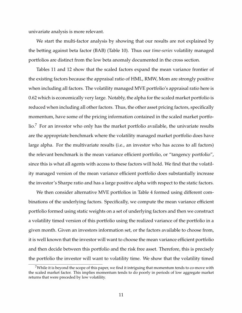
Tables 11 and 12 show that the scaled factors expand the mean variance frontier of

the existing factors because the appraisal ratio of HML, RMW, Mom are strongly positive

when including all factors. The volatility managed MVE portfolio’s appraisal ratio here is

0.62 which is economically very large. Notably, the alpha for the scaled market portfolio is

reduced when including all other factors. Thus, the other asset pricing factors, specifically

momentum, have some of the pricing information contained in the scaled market portfo-

lio.7 For an investor who only has the market portfolio available, the univariate results

are the appropriate benchmark where the volatility managed market portfolio does have

large alpha. For the multivariate results (i.e., an investor who has access to all factors)

the relevant benchmark is the mean variance efficient portfolio, or “tangency portfolio”,

since this is what all agents with access to these factors will hold. We find that the volatil-

ity managed version of the mean variance efficient portfolio does substantially increase

the investor’s Sharpe ratio and has a large positive alpha with respect to the static factors.

We then consider alternative MVE portfolios in Table 4 formed using different com-

binations of the underlying factors. Specifically, we compute the mean variance efficient

portfolio formed using static weights on a set of underlying factors and then we construct

a volatility timed version of this portfolio using the realized variance of the portfolio in a

given month. Given an investors information set, or the factors available to choose from,

it is well known that the investor will want to choose the mean variance efficient portfolio

and then decide between this portfolio and the risk free asset. Therefore, this is precisely

the portfolio the investor will want to volatility time. We show that the volatility timed

7While it is beyond the scope of this paper, we find it intriguing that momentum tends to co-move withthe scaled market factor. This implies momentum tends to do poorly in periods of low aggregate marketreturns that were preceded by low volatility.

11

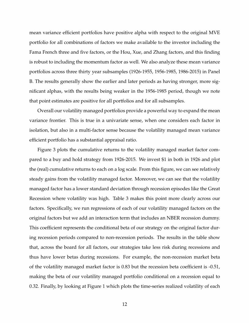
mean variance efficient portfolios have positive alpha with respect to the original MVE

portfolio for all combinations of factors we make available to the investor including the

Fama French three and five factors, or the Hou, Xue, and Zhang factors, and this finding

is robust to including the momentum factor as well. We also analyze these mean variance

portfolios across three thirty year subsamples (1926-1955, 1956-1985, 1986-2015) in Panel

B. The results generally show the earlier and later periods as having stronger, more sig-

nificant alphas, with the results being weaker in the 1956-1985 period, though we note

that point estimates are positive for all portfolios and for all subsamples.

Overall our volatility managed portfolios provide a powerful way to expand the mean

variance frontier. This is true in a univariate sense, when one considers each factor in

isolation, but also in a multi-factor sense because the volatility managed mean variance

efficient portfolio has a substantial appraisal ratio.

Figure 3 plots the cumulative returns to the volatility managed market factor com-

pared to a buy and hold strategy from 1926-2015. We invest $1 in both in 1926 and plot

the (real) cumulative returns to each on a log scale. From this figure, we can see relatively

steady gains from the volatility managed factor. Moreover, we can see that the volatility

managed factor has a lower standard deviation through recession episodes like the Great

Recession where volatility was high. Table 3 makes this point more clearly across our

factors. Specifically, we run regressions of each of our volatility managed factors on the

original factors but we add an interaction term that includes an NBER recession dummy.

This coefficient represents the conditional beta of our strategy on the original factor dur-

ing recession periods compared to non-recession periods. The results in the table show

that, across the board for all factors, our strategies take less risk during recessions and

thus have lower betas during recessions. For example, the non-recession market beta

of the volatility managed market factor is 0.83 but the recession beta coefficient is -0.51,

making the beta of our volatility managed portfolio conditional on a recession equal to

0.32. Finally, by looking at Figure 1 which plots the time-series realized volatility of each

12

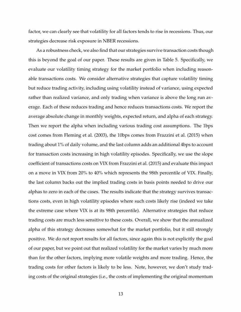
factor, we can clearly see that volatility for all factors tends to rise in recessions. Thus, our

strategies decrease risk exposure in NBER recessions.

As a robustness check, we also find that our strategies survive transaction costs though

this is beyond the goal of our paper. These results are given in Table 5. Specifically, we

evaluate our volatility timing strategy for the market portfolio when including reason-

able transactions costs. We consider alternative strategies that capture volatility timing

but reduce trading activity, including using volatility instead of variance, using expected

rather than realized variance, and only trading when variance is above the long run av-

erage. Each of these reduces trading and hence reduces transactions costs. We report the

average absolute change in monthly weights, expected return, and alpha of each strategy.

Then we report the alpha when including various trading cost assumptions. The 1bps

cost comes from Fleming et al. (2003), the 10bps comes from Frazzini et al. (2015) when

trading about 1% of daily volume, and the last column adds an additional 4bps to account

for transaction costs increasing in high volatility episodes. Specifically, we use the slope

coefficient of transactions costs on VIX from Frazzini et al. (2015) and evaluate this impact

on a move in VIX from 20% to 40% which represents the 98th percentile of VIX. Finally,

the last column backs out the implied trading costs in basis points needed to drive our

alphas to zero in each of the cases. The results indicate that the strategy survives transac-

tions costs, even in high volatility episodes where such costs likely rise (indeed we take

the extreme case where VIX is at its 98th percentile). Alternative strategies that reduce

trading costs are much less sensitive to these costs. Overall, we show that the annualized

alpha of this strategy decreases somewhat for the market portfolio, but it still strongly

positive. We do not report results for all factors, since again this is not explicitly the goal

of our paper, but we point out that realized volatility for the market varies by much more

than for the other factors, implying more volatile weights and more trading. Hence, the

trading costs for other factors is likely to be less. Note, however, we don’t study trad-

ing costs of the original strategies (i.e., the costs of implementing the original momentum

13

strategy as opposed to the volatility managed version).

We also consider strategies that impose leverage constraints. A simple strategy is

one that only updates the portfolio when volatility is above it’s mean value. This port-

folio both trades less frequently and also avoids the use of leverage from low volatility

episodes where the risk weight would normally rise substantially. In unreported results,

we find such constraints weaken the strategies considered, but not substantially so. There

are still large alphas and substantial gains in Sharpe ratios.

As an additional robustness check, we demonstrate that our results hold when study-

ing 20 OECD countries and focus on the broad stock market indices of each country. On

average, the managed volatility version of the index has an annualized Sharpe ratio that

is 0.15 higher than a passive buy and hold strategy, representing a substantial increase.

The volatility managed index has a higher Sharpe ratio than the passive strategy in 80%

of cases. These results are detailed in Figure 6 of our Appendix. Note that is a strong

condition – a portfolio can still have positive alpha even when it’s Sharpe ratio is below

the non-managed factor. The main text is devoted to understanding the better studied US

factors.

3.3 Understanding the profitability of volatility timing

We first give intuition for why our volatility managed portfolios work in terms of gener-

ating positive risk adjusted returns. Then, we discuss how to reconcile these results with

the return predictability literature. At first, it may sound contradictory that our volatility

portfolios decrease risk exposure after large market downturns when volatility increases,

as confirmed by Table 3 which shows low recession betas of our factor. These are times

when we think expected returns are rising. We show that the frequency of these two

variables behave quite differently. Volatility tends to spike and recede quickly whereas

expected returns are more persistent. This reconciles the two findings.

We start by showing that volatility for each factor doesn’t predict the factor’s future re-

14

turns. We run monthly regressions of future 1 month returns on monthly realized volatil-

ity for each factor. Using log realized volatility or using realized variance does not change

these results.

Table 2 gives these results. We can see that coefficients across factors range from pos-

itive to negative but are, generally speaking, not significant. Therefore, we don’t see any

clear relationship between a factors’ volatility and its future expected return. Mechani-

cally, this is why the strategy we implement works. If a factors volatility does not predict

an increase in returns, then an increase in volatility signifies a poor risk return tradeoff

where reducing risk exposure is optimal. Our appendix maps this out more clearly by

showing the exact conditions under which our strategy generates alpha. But, intuitively,

the lack of risk return tradeoff in the data means volatility timing will be profitable.

Next, we try to understand our results in light of the return predictability literature.

To better understand the co-movement between expected returns and conditional vari-

ance in the data, we estimate a VAR for expected returns and variances of the market

portfolio. We then trace out the portfolio choice implications for a myopic mean variance

investor to a volatility shock. We set risk aversion just above 2, where our choice is set

so that the investor holds the market on average when using the unconditional value for

variance and the equity premium (i.e., in the absence of movements in expected returns

and vol, the portfolio weight is w = 1). This gives a natural benchmark to compare to.

The VAR first estimates the conditional mean and conditional variance of the market

return using monthly data on realized variance, monthly market returns, the monthly

(log) price to earnings ratio, and the BaaAaa default spread. The expected return is

formed by using the fitted value from a regression of next months stock returns on the

price to earnings ratio, default spread, and realized variance (adding additional lags of

each does not change results).

Expected variance is formed using a log normal model for volatility and including 3

15

lags for each factors realized volatility.

ln RVt+1 = a +J

∑j=1

ρj ln RVt−j−1 + cxt + εt+1 (2)

For each factor we include three monthly lags of its own realized variance so J = 3, and

we include the log market variance as a control (note: this would be redundant for the

market itself). We plan to explore additional controls in the future, though we note the

regressions generally produce a reasonably high R-square. We can then form conditional

expectations of future volatility or variance or inverse variance easily from our log speci-

fication. Taking conditional expectations forms our forecasts; specifically

σnt = Et[RVn

t+1] = exp

(n

(a +

J

∑j=1

ρj ln RVt−j−1 + cxt

)+

n2

2σ2

ε

)

We can then set n = 1/2, 1 as our forecast of volatility or variance, respectively. The last

term in the above equation takes into account a Jensen’s inequality effect.

We then take the estimated conditional expected return and variance and run a VAR

with 3 lags of each variable. We consider the effect of a variance shock where we choose

the ordering of the variables so that the variance shock can affect contemporaneous ex-

pected returns as well. These results are meant to be somewhat stylized in order to un-

derstand our claims about portfolio choice when expected returns also vary and to under-

stand the intuition for how portfolio choice should optimally respond to a high variance

shock.

The results are given in Figure 2. We see that a variance shock raises future variance

sharply and immediately. Expected returns, however, do not move much on impact but

rise slowly as time goes on. The impulse response for the variance dies out fairly quickly,

consistent with variance being strongly mean reverting. Given the increase in variance

but only slow increase in expected return, the lower panel shows that it is optimal for

the investor to reduce his portfolio exposure from 1 to 0.6 on impact because of an unfa-

vorable risk return tradeoff. This is because expected returns have not risen fast enough

16

relative to volatility. The portfolio share is consistently below 1 for roughly 18 months af-

ter the shock. At this point, variance decreases enough and expected returns rise enough

that an allocation above 1 is desirable. This increase in risk exposure fades very slowly

over the next several years. These results square our findings with the portfolio choice

literature. They say that in the face of volatility spikes expected returns do not react imme-

diately and at the same frequency. This suggests reducing risk exposures by substantial

amounts at first. However, the investor should then take advantage of favorable increases

in expected returns once volatility has return to reasonable levels.

It is well known that both movements in stock-market variance and expected returns

are counter-cyclical (French et al. (1987), Lustig and Verdelhan (2012)). Here, we show that

the much lower persistence of volatility shocks implies the risk-return trade-off initially

deteriorates but gradually improves as volatility recedes through the recession. Thus, our

volatility timing results are not in conflict with expected return timing results. Instead,

after a large market crash such as October 2008, our strategy says to get out immediately

to avoid an unfavorable risk return tradeoff, but by buying back in when the volatility

shock subsides, one can capture much of the expected return increase.

We further push this intuition in Figure 4 where we show the behavior of our volatility

timing strategy during four prominent market downturns: the Great Depression, the 2008

recession, the 1987 stock market crash, and the oil crisis and stock market downturn of

1974-1975. In all episodes one can see our strategy decreasing risk exposure after the

initial decline in the market, and gradually increasing risk exposure as the episode moves

on.

4. Portfolio choice implications

In this section, we focus on understanding the implications for portfolio choice of our

findings. We start by computing the utility gain of volatility timing for a mean-variance

investor, and find that these gains to be substantially larger that utility gains arising from

17

standard expected return timing strategies. We then study the portfolio problem of a

long-horizon investor.

Here we focus on the portfolio problem of an investor that trades one risky portfolio

and risk-free bond, and calibrate the parameters in our analysis to be consistent with the

market portfolio. Our results for the mean-variance investor in Section 4.1 extend directly

to the other portfolios considered in Section 3, and specifically they carry over for the ex-

post tangency portfolio. Our results for a long-horizon investor in Section 4.2 rely much

more heavily on the vast literature on return predictability for the aggregate market, and

can be extended to the other factors if one is willing to take a stand on the composition

of cash-flow and discount-rate shocks for these factors, and how this composition varies

over-time. To the extent that these factors behave like the market, our results should carry

over as well.

4.1 The benefits of volatility timing for a mean-variance investor

We now use simple mean-variance preferences to give a sense of the benefits of timing

fluctuations in conditional factor volatility. For simplicity we focus on a single factor. For

our numerical comparisons we will use the market as the factor though we emphasize

that our volatility timing works well for other factors as well. In particular our goal

here is to compare directly the benefits of volatility timing and expected return timing.

Specifically, we extend the analysis in Campbell and Thompson (2008) to allow for time-

variation in volatility.

4.1.1 Expected return timing

Consider the following excess return process,

rt+1 = µ + xt +√

Ztet+1 (3)

where E[xt] = E[et] = 0 and xt, et+1 are conditionally independent. We begin by

studying an investor who follows an unconditional strategy and an expected return tim-

18

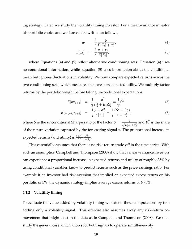
ing strategy. Later, we study the volatility timing investor. For a mean-variance investor

his portfolio choice and welfare can be written as follows,

w =1γ

µ

E[Zt] + σ2x

; (4)

w(xt) =1γ

µ + xt

E[Zt]; (5)

where Equations (4) and (5) reflect alternative conditioning sets. Equation (4) uses

no conditional information, while Equation (5) uses information about the conditional

mean but ignores fluctuations in volatility. We now compare expected returns across the

two conditioning sets, which measures the investors expected utility. We multiply factor

returns by the portfolio weight before taking unconditional expectations:

E[wrt+1] =1γ

µ2

σ2x + E[Zt]

=1γ

S2 (6)

E[w(xt)rt+1] =1γ

µ + σ2x

E[Zt]=

1γ

(S2 + R2r )

1− R2r

, (7)

where S is the unconditional Sharpe ratio of the factor S = µ√E[Zt]+σ2

xand R2

r is the share

of the return variation captured by the forecasting signal x. The proportional increase in

expected returns (and utility) is 1+S2

S2R2

r1−R2

r.

This essentially assumes that there is no risk-return trade-off in the time-series. With

such an assumption Campbell and Thompson (2008) show that a mean-variance investors

can experience a proportional increase in expected returns and utility of roughly 35% by

using conditional variables know to predict returns such as the price-earnings ratio. For

example if an investor had risk-aversion that implied an expected excess return on his

portfolio of 5%, the dynamic strategy implies average excess returns of 6.75%.

4.1.2 Volatility timing

To evaluate the value added by volatility timing we extend these computations by first

adding only a volatility signal. This exercise also assumes away any risk-return co-

movement that might exist in the data as in Campbell and Thompson (2008). We then

study the general case which allows for both signals to operate simultaneously.

19

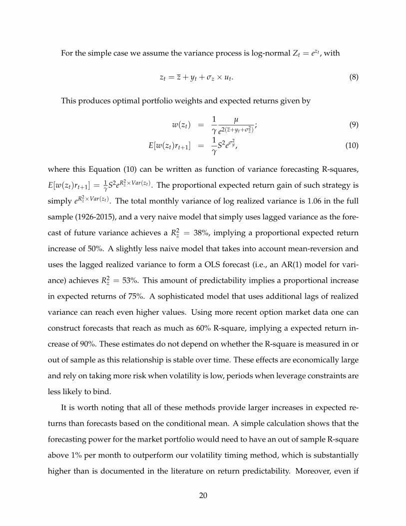
For the simple case we assume the variance process is log-normal Zt = ezt , with

zt = z + yt + σz × ut. (8)

This produces optimal portfolio weights and expected returns given by

w(zt) =1γ

µ

e2(z+yt+σ2z)

; (9)

E[w(zt)rt+1] =1γ

S2eσ2y , (10)

where this Equation (10) can be written as function of variance forecasting R-squares,

E[w(zt)rt+1] =1γ S2eR2

z×Var(zt). The proportional expected return gain of such strategy is

simply eR2z×Var(zt). The total monthly variance of log realized variance is 1.06 in the full

sample (1926-2015), and a very naive model that simply uses lagged variance as the fore-

cast of future variance achieves a R2z = 38%, implying a proportional expected return

increase of 50%. A slightly less naive model that takes into account mean-reversion and

uses the lagged realized variance to form a OLS forecast (i.e., an AR(1) model for vari-

ance) achieves R2z = 53%. This amount of predictability implies a proportional increase

in expected returns of 75%. A sophisticated model that uses additional lags of realized

variance can reach even higher values. Using more recent option market data one can

construct forecasts that reach as much as 60% R-square, implying a expected return in-

crease of 90%. These estimates do not depend on whether the R-square is measured in or

out of sample as this relationship is stable over time. These effects are economically large

and rely on taking more risk when volatility is low, periods when leverage constraints are

less likely to bind.

It is worth noting that all of these methods provide larger increases in expected re-

turns than forecasts based on the conditional mean. A simple calculation shows that the

forecasting power for the market portfolio would need to have an out of sample R-square

above 1% per month to outperform our volatility timing method, which is substantially

higher than is documented in the literature on return predictability. Moreover, even if

20

some variables are able to predict conditional expected returns above this threshold, it is

not clear if an investor would have knowledge and access to these variables in real time.

In contrast, data on volatility is much simpler and more available. Even a naive investor

who simply assumes volatility next month is equal to realized volatility last month will

outperform a expected return timing strategy in terms of utility gain.

Importantly, volatility timing can be implemented not only for the aggregate market,

but for the several additional factors studied in Section 3, with similar degrees of success.

The degree of predictability we find for the conditional variance of different factors is

fairly similar, with simple AR(1) models generally producing R-square values around

50-60% at the monthly horizon. In contrast, the same variables that help forecast mean

returns on the aggregate market portfolio do not necessarily apply to other portfolios

such as value, momentum, or the currency carry trade. Thus, we would need to come

up with additional return forecasting variables for each of the different factors. Volatility

timing on the other hand is easy to replicate across factor because lags of the factors own

variance is a very reliable and stable way to estimate conditional expected variance across

factors.

Nevertheless one needs to be cautious with these magnitudes. The same caveat that

applied to Campbell and Thompson (2008) applies here as well. Specifically, it is possible

that co-movement between xt and zt erases much of these gains.

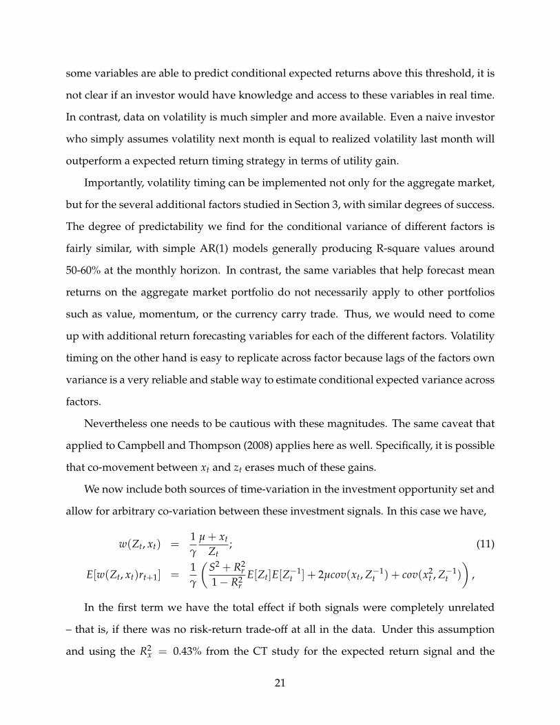
We now include both sources of time-variation in the investment opportunity set and

allow for arbitrary co-variation between these investment signals. In this case we have,

w(Zt, xt) =1γ

µ + xt

Zt; (11)

E[w(Zt, xt)rt+1] =1γ

(S2 + R2

r1− R2

rE[Zt]E[Z−1

t ] + 2µcov(xt, Z−1t ) + cov(x2

t , Z−1t )

),

In the first term we have the total effect if both signals were completely unrelated

– that is, if there was no risk-return trade-off at all in the data. Under this assumption

and using the R2x = 0.43% from the CT study for the expected return signal and the

21

more conservative R2z = 53% for the variance signal, one would obtain a 236% increase

in expected returns. But there is some risk-return trade-off in the data, thus we need to

consider the other terms as well.

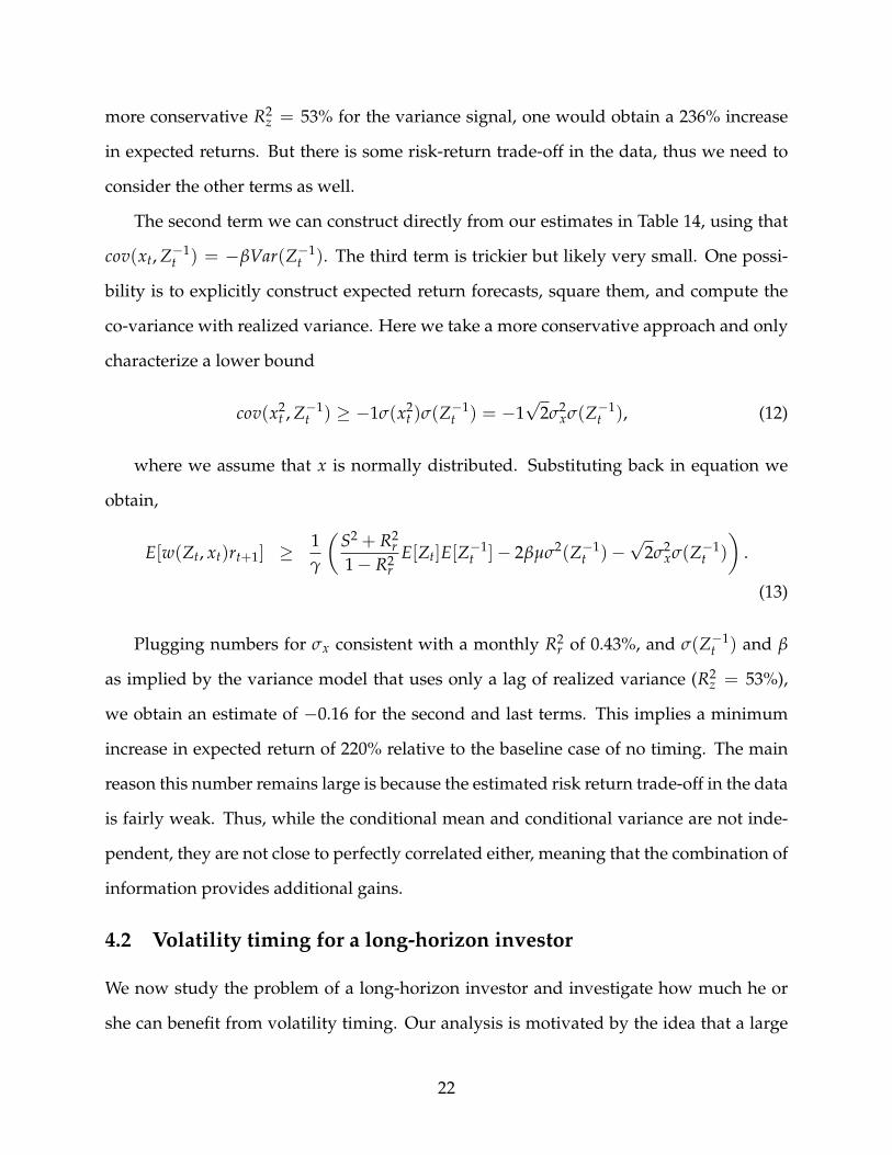
The second term we can construct directly from our estimates in Table 14, using that

cov(xt, Z−1t ) = −βVar(Z−1

t ). The third term is trickier but likely very small. One possi-

bility is to explicitly construct expected return forecasts, square them, and compute the

co-variance with realized variance. Here we take a more conservative approach and only

characterize a lower bound

cov(x2t , Z−1

t ) ≥ −1σ(x2t )σ(Z−1

t ) = −1√

2σ2xσ(Z−1

t ), (12)

where we assume that x is normally distributed. Substituting back in equation we

obtain,

E[w(Zt, xt)rt+1] ≥1γ

(S2 + R2

r1− R2

rE[Zt]E[Z−1

t ]− 2βµσ2(Z−1t )−

√2σ2

xσ(Z−1t )

).

(13)

Plugging numbers for σx consistent with a monthly R2r of 0.43%, and σ(Z−1

t ) and β

as implied by the variance model that uses only a lag of realized variance (R2z = 53%),

we obtain an estimate of −0.16 for the second and last terms. This implies a minimum

increase in expected return of 220% relative to the baseline case of no timing. The main

reason this number remains large is because the estimated risk return trade-off in the data

is fairly weak. Thus, while the conditional mean and conditional variance are not inde-

pendent, they are not close to perfectly correlated either, meaning that the combination of

information provides additional gains.

4.2 Volatility timing for a long-horizon investor

We now study the problem of a long-horizon investor and investigate how much he or

she can benefit from volatility timing. Our analysis is motivated by the idea that a large

22

fraction of stock price movements are transitory, implying that stock market volatility

might not be the relevant measure of risk for a long-horizon investor.

Formally, the idea is that changes in volatility might be mostly driven by discount rate

volatility. A high discount rate volatility means that you might wake-up poorer tomor-

row, but expected returns moved exactly so you expect to be just as rich fifty years from

now. Thus, according to this view increases in volatility does not pose a risk to a long

run investor because these discount rate shocks wash out in the long run. John Cochrane

articulates this view nicely in a 2008 Wall Street Journal article:

And what about volatility?(...) if you were happy with a 50/50 portfolio

with an expected return of 7% and 15% volatility , 50% volatility means you

should hold only 4.5% of your portfolio in stocks! (...) expected returns would

need to rise from 7% per year to 78% per year to justify a 50/50 allocation with

50% volatility. (...) The answer to this paradox is that the standard formula

is wrong. (...) Stocks act a lot like long-term bonds – when prices decline

and dividend yields rise, subsequent returns rise as well.(...)If bond prices go

down more, bond yields and long-run returns will rise just enough that you

face no long-run risk.(...)the same logic explains why you can ignore ”short-

run” volatility in stock markets.

Our goal here is to understand better this advice: how long-run an investment hori-

zon needs to be for investors to safely ignore discount rate volatility? We find that only

extremely long run investors can safely ignore discount rate volatility. For example, we

show that even an investor with a 30 year horizon still cares about discount rate volatil-

ity and finds it optimal to reduce his portfolio weight when volatility goes up. The key

for this result is that, in the data, shocks to expected returns seem to be very persistent,

so an investor has to be indifferent with respect to fluctuations in the value of his or her

wealth for many years in the future. To the extent that these expected returns were less

23

persistent, long horizon investors would perceive increases in discount rate volatility as

less risky.

Earlier work on portfolio choice has studied expected return variation, volatility vari-

ation, or volatility variation with a constant risk-return trade-off.8 In order to understand

how much long-horizon investor can benefit from the empirical patterns we document

in the data, we solve the dynamic portfolio problem in a stochastic environment that (i)

allows for independent variation in expected returns and volatility; and (ii) allows for

variation in the mix of cash-flow and discount-rate shocks. These two ingredients are

novel and essential to interpret our findings.

We now discuss the assumed stochastic environment, followed by investors prefer-

ences, and a brief description of the portfolio optimization problem. Our interest is quan-

titative, so we focus on contrasting how the long-horizon investor responds differently to

time-variation in volatility.

4.2.1 Investment opportunity set

We assume there are two assets. A risk-less bond that pays constant interest rate rdt, and

risky asset St, with dynamics given by

dSt

St= (r + xt)dt +

√ytDdBt + FdZt, (14)

where St is the value of a portfolio fully invested in the asset and that reinvests all

dividends, xt is a scalar that drives the risky asset excess return, and yt is a scalar that

drives variation in return volatility. The shocks dBt and dZt are independent three di-

mensional Brownian motions. An important innovation in our analysis is to allow the

mix of volatility to vary, what happens as long as F and D are not proportional to each

other.8Example of work that study volatility timing in a dynamic environment are Chacko and Viceira (2005)

and Liu (2007).

24

The state variables evolve as follows,

dxt = κx(µx − xt)dt +√

ytGdBt + HdZt (15)

dyt = κy(µy − yt)dt +√

ytLdBt. (16)

The volatility process follows a CIR process as in Heston (1993), so it is bounded

below by zero. We impose the appropriate conditions to guarantee that the zero boundary

is reflexive (2κyµy > L′L). Vectors D, F, G, H, L are three by one constant vectors, κx, κy

are positive scalars that control the rate of mean-reversion of discount rate and volatility

shocks, and µx, µy are the unconditional averages of expected returns and volatility.

The vectors G and H have the the first two rows equal to zero. So only the third

shock of each Brownian moves discount rates. The fact that discount rate shocks only

have a transitory effect on asset prices implies G[3] = −D[3]κx = and H[3] = −F[3]κx.

The vector L has the first entry equal to zero. The second entry captures pure volatility

shocks that are contemporaneously unrelated to discount rate shocks, and the third entry

captures the fact that volatility and expected returns might go up at the same time. The

vectors D and F have in the first two entries permanent cash-flow shocks. In the first

entry we have the exposure to shocks unrelated to volatility or expected returns, and in

the second shocks related to volatility. In the third entry we have the discount rate shocks.

Shocks that by construction mean-revert in the long run.

Two features of this environment are important for our analysis. First, this specifica-

tion allows flexibility to fit the weak relationship between expected returns and volatility

we see in the data. Expected returns and volatility can potentially co-move by making

|L′G| > 0 but they don’t need to. Second, the specification allow us flexibility to choose

both the average mix of discount rate and cash-flow shocks, and how the distribution of

these shocks evolve over time. In particular, we consider extreme cases where all time-

variation in volatility is driven by discount rate volatility.

25

4.2.2 Investor preferences and optimization

Investors preferences are described by Epstein and Zin (1989) utility. We adopt the Duffie

and Epstein (1992) continuous time implementation:

J = Et

[∫ ∞

tf (Cs, Js)ds

](17)

f (C, J) = ρ1− γ

1− ψ−1 J ×

( C

((1− γ)J)1

1−γ

)1−ψ−1

− 1

(18)

where ρ is rate of time preference, γ the coefficient of relative risk aversion, and ψ

is the elasticity of intertemporal substitution. Power utility is the knife edge case where

γ = ψ−1. In the limit ψ→ 1, the aggregator f (C, J) converges to

f (C, J) = ρ(1− γ)J ×[

log(C)− log((1− γ)J)1− γ

]. (19)

Let Wt denote the investor wealth and wt the allocation to the risky asset, then his

budget constraint can be written as,

dWt

Wt= [wtxt + r− Ct

Wt]dt + wt

√ytDdBt + wtFdZt. (20)

The investor maximizes 17 subject to his intertemporal budget constraint and the evo-

lution of state variables xt and yt.

4.2.3 Solution

The optimization problem has three state variable. The investor wealth plus the two

drivers (expected return x and volatility y) of the investment opportunity set. The Bell-

man equation for this problem is

0 = supw,C f (Ct, Jt) + [wtxtWt + rWt − Ct]JW + 12 w2

t W2t JWW (ytD′D + F′F)

+ κy(µy − yt)Jy +12Yt JyyL′L + κx(µx − xt)Jx +

12 Jxx(ytG′G + H′H)

+ yt JxyG′L + wtWt JxW(G′Dyt + F′H) + wtWt JyW L′DYt (21)

This problem can be simplified to two state variable by exploring homogeneity of the

problem with respect to wealth. In particular, a function of the form J(W, x, Y) = W1−γ

1−γ eV(x,y)

26

satisfies the above equation. We use collocation methods to solve this problem numeri-

cally.

To get intuition about the results that follow it is useful to stare at the optimal portfolio

policy,

wt =xt

γ (D′Dyt + F′F)+ Vx

G′Dyt + F′Hγ (D′Dyt + F′F)

+ VyL′Dyt

γ (D′Dyt + F′F). (22)

The first term is the myopic demand, which reflects the portfolio choice of a short-horizon

investor. The two additional terms are the Mertonian hedging demands. Past studies of

volatility timing have focused on the third term, which is important to the extent that

volatility innovations are strongly correlated with returns. Chacko and Viceira (2005)

shows that for parameters consistent with the data, this term turn out not to be quanti-

tatively important. The return predictability literature has emphasized the second term.

The fact that expected returns tend to increase after low returns, make investment in the

risky asset a natural investment opportunity set hedge. This effects leads to a higher av-

erage position in the the risky asset (Vx is typically negative). Our analysis emphasizes

how the strength of this hedging demand fluctuates with volatility.

Assuming for illustration purposes that L′D = 0, we can write

wt =xt

γ (D′Dyt + F′F)− κxVx

DRshare(yt)

γ, (23)

where DRshare(yt) =G′Dyt+F′H

κx(D′Dyt+F′F) is the share of return volatility which is driven by dis-

count rate shocks. If most variation in volatility is about discount rate volatility, than

DRshare(yt) will be high in periods of high volatility. This increase in the discount rate

share will tend to increase the hedging demand in periods of high volatility, counteract-

ing the myopic demand, which calls for a reduction in position.This is the effect John

Cochrane alludes to in the previous quote.

Investment horizon plays a role in equation (23) through Vx, the sensitivity of the

investor value function with respect to the expected return state variable. A long horizon

implies the investor can benefit more from the variation in expected returns, increasing

27

hedging demands accordingly. Intuitively, the risky asset is a better hedge for a long-

horizon investor because he or she can wait until the price recovers after a increase in

discount rates.

Note that the same force that makes long-horizon investors less responsive to changes

in volatility driven by discount rates, will make them more responsive to time-variation

in volatility when the driver is cash flow volatility. In this case,DRshare(yt) will be low in

periods of high volatility, further reinforcing the myopic demand. In the case the mix of

shocks is constant (F ∝ D and G ∝ H), the optimal policy only deviates from the myopic

policy to the extent that Vx changes with yt.

The analysis that follows is focused on understanding how large is Vx and how Vx

changes with the volatility state variable yt.

4.2.4 Analysis

We study alternative calibrations of the return process that vary in the composition of

volatility shocks. Our focus here is to show that in this fairly rich environment the optimal

portfolio response of the long-horizon investor with respect to changes in volatility can

be approximately described by a strategy that is a constant weight combination of the

buy-and-hold portfolio and the volatility managed portfolio.

Table 8 reports the moments used in our calibration. Calibration (a) is the case in

which fluctuations in volatility are driven by changes in the volatility of the permanent

shock to prices (cash-flow volatility). In calibration (b) we study the case where all time-

variation in volatility is the result of variation in the volatility of shocks that have a transi-

tory effect on prices (discount rate volatility). Calibration (c) studies the case of a constant

mix of transitory and permanent shocks, where changes in volatility do not change the

relative importance of permanent and transitory shocks.

We calibrate the stochastic processes to be consistent with the following moments:

average volatility, the R-square of a predictability regression of year-ahead returns on the

28

price-dividend ratio, the auto-correlation coefficient of the logarithm of realized variance,

the standard deviation of the logarithm of realized variance, and the auto-correlation of

the expected return process.

We study CRRA preferences with risk aversion of 5 and 10, and Esptein and Zin utility

with with risk aversion of 5 and 10, and IES of 0.5, 1 and 1.5. Following the analysis in

Blanchard (1985) and Garleanu and Panageas (2015), we use the preference parameter ρ

as a proxy for investor horizon. We choose ρ so that the half-life9 of utility weights ranges

from 5 year to 30 years.

To focus on the effects of volatility variation we initially abstract from subtle hedg-

ing demand effects arising from any contemporaneous correlation between return and

volatility shocks and set D[2] = 0, and assume zero correlation between volatility and

expected return shocks L[3] = 0. Chacko and Viceira (2005) studies the effect of such

hedging demands and show that the effects are small for plausible levels of risk-aversion.

We will later revisit these assumptions.

We are interested in understanding how much a long-horizon investor deviate from

the optimal mean-variance portfolio. To focus on the effect of volatility we fit the fol-

lowing linear relation on the optimal policy evaluated at the unconditional equity premia

w∗(µx, yt) = a + b × 1D′Dyt+F′F . The policies of a mean-variance investor fit this linear

relation perfectly with a = 0 and b =µxγ . In short, the mean-variance investor puts zero

weight on the buy-and-hold portfolio and weight 1 on the volatility managed portfolio.

In Tables 6 (a-c) we report b× γµx

, so the reported coefficients have the direct interpretation

of how much weight the investor places on the volatility managed portfolio. A coefficient

lower than one implies the long-horizon investor trades volatility less aggressively than

the mean-variance investor. In the last column we give the minimum R-square across

specifications in a given row where the row denotes investor horizon. Overall, we see

9Specifically we map horizon into ρ as follows: For a given horizon Tj, look for ρj such that∫ Tj

0 e−ρj×tdt∫ ∞0 e−ρj×tdt

=

12

29

that the linear relation fits the optimal policy extremely well.

Table 6(a) shows the case where all time-variation in volatility is driven by cash-flow

volatility. The long-horizon investor responds more aggressively than the mean-variance

investor (weight on the volatility managed portfolio is higher than one). Intuitively,

when cash-flow volatility goes down, the proportion of discount-rate shocks to cash-flow

shocks decreases, making stocks relatively safer for a long-horizon investor. Thus, the

long-horizon investor responds by increasing his portfolio allocation more than propor-

tionally with the decrease in variance. Importantly this does not speak to their average

positions on the risky asset, but only speak to how positions change with volatility.

Table 6(b) shows the case where the average mix is consistent with the data, but all

time-variation in volatility is discount rate volatility. For example, both John Cochrane

(2008)10 and Warren Buffet(2008)11 interpreted the massive increase in volatility in the

fall of 2008 as mostly about discount rate volatility and based on that they argued that it

was a good time to buy for a long-horizon investor. The linear policy is still an almost

perfect description of the optimal policy, but now long-horizon investors respond less ag-

gressively to changes in volatility. Consistent with the intuition in Buffet and Cochrane,

long-horizon investors do trade less aggressively on changes in discount rate volatility,

but inconsistent with their views a long-horizon investor still trades quite a bit. Coeffi-

cients are always quite high, implying that the dynamic investor invests quite a bit on

the volatility managed portfolio. For example,during the fall of 2008 volatility spiked

from 20% to 60%. This would induce the mean-variance investor to shrinks his weight by

90%, while an investor with half-life of 30 years and coefficient of relative risk-aversion

5, would shrink his portfolio by 42%(0.47*90%). This aggressive response to discount

rate volatility is at odds with the view expressed by Buffet and Cochrane. Long-horizon

investors perceive discount-rate volatility as risky because measured discount-rate varia-

tion is extremely persistent in the data. Even though shocks eventually mean-revert, they

10WSJ, Nov/2008 ”Is now the time to buy stocks?”11NYT, Oct/2008 ”Buy American. I am.”

30

take a long time.

Table 6(c) shows the case where the average mix of discount-rate and cash-flow volatil-

ity is constant. This is a natural benchmark given that we are not aware of any work that

have shown how the mix of discount rate and volatility shocks evolve over-time in a

predictable way. Again coefficients are basically equal to 1. The mean-variance policy

is still a good description of how the long-horizon investor should change his portfolio.

Obviously the presence of discount rate shocks will induce the long-horizon investor to

perceive less risk and hold more stocks on average, but his response to changes in volatil-

ity is approximately equal to the mean-variance investor behavior.

In Tables 7 (d) and (e) we study the effect of introducing contemporaneous correlation

between return realizations and volatility innovations. Chacko and Viceira (2005) stud-

ies the hedging demands that result from this correlation. Here our focus is not in level

effects on the investor allocation, but whether these correlations change how an investor

should respond to volatility shocks. We start from calibration (c) and introduce a corre-

lation between realized returns and volatility shocks. In Table 7 (d) is the case where the

correlation between returns and volatility is entirely due to the discount rate component.

That is volatility and expected returns shock are positively related in this case. Table 7 (e)

analyzes the other extreme where none of the correlation between returns and volatility

is due to the discount rate component. In this case the expected return process is again

completely independent of the discount rate volatility process. In both cases we see that

the introduction of this correlation did not meaningfully change how investors respond

to changes in volatility. As is was the case for calibration (c) the long-horizon investor

responds roughly in the same fashion as the mean-variance investors

4.2.5 Summary

Overall, this analysis shows that long horizon investors can substantially benefit from

volatility timing, and their optimal policy can be described by a simple strategy that com-

31

bines the buy-and-hold and the volatility managed portfolio.

The distinction between the type of volatility that is time-varying plays an important

role in determining how much a long-horizon investor weights the volatility managed

portfolio. Specifically we distinguish between volatility of cash flow shocks, shocks that

have permanent effects on the level of prices, and volatility of discount rate shocks, shocks

that have only transitory effects on the price level.

This distinction interacts with the investor horizon in an interesting fashion. In partic-

ular, long-horizon investors are better able to deal with discount rate volatility. Cash-flow

volatility on the other hand impacts all investors equally because there are permanent

shocks to asset prices.

We find that only when all variation in volatility is driven by discount rate volatility,

the long horizon investor responds less aggressively to changes in volatility. But even in

this case, the optimal weight on the volatility managed portfolio is positive and substan-

tial for horizons up to 30 years.

5. Implications for economic theory

This section sketches the implications of our empirical results for theories of time-varying

risk-premia. We have in mind theories based on habit formation (Campbell and Cochrane,

1999), long-run risk (Bansal and Yaron, 2004), intermediaries (He and Krishnamurthy,

2012), and rare disasters (Wachter, 2013).

First, we want to acknowledge that these models were not designed to think about

the cross-section of asset prices, and we are mindful that theories linking macro and asset

prices are typically designed to think about lower frequencies than the studied in this

paper. Here our goal is to briefly contrast the empirical pattern we document in the data

with these models predictions.

Specifically, our results speak to these theories because their aim is to explain time-

variation in risk-premia through a combination of time-variation in risk and the price of

32

risk. Our empirical work allow us to study whether the joint dynamics these models rely

on is consistent with the data, at least at the frequencies that we study.

In He and Krishnamurthy (2012) (HK) and Campbell and Cochrane (1999) (CC) time-

variation in risk and the price of risk is endogenous and a function of past shocks. In

these models,

maxi

Et[Rei,t+1]

σ2t (Re

i,t+1)≈ f (st) (24)

where f ′(st) < 0,and st is a state variable that is an increasing function of past shocks

to consumption. In both these models past consumption shocks shape the sensitivity of

the marginal utility to future consumption shocks.12 In both these economies, negative

shocks to consumption makes marginal utility volatile, resulting in an endogenous in-

crease in asset price volatility. So any asset with a positive risk-premia will also feature

an endogenous increase in it’s return volatility in periods where the price of risk is high.

Another paper with this feature is Barberis et al. (2001) who have effective risk aversion

occurring after realized losses.

While it is undisputed that the data features a lot of excess volatility, these models

seem to generate volatility at the wrong times. In the data periods of higher than average

volatility are associated with periods of lower than average price of risk.

Wachter (2013) and Bansal and Yaron (2004) have a different flavor as they rely on

time variation in cash-flow risk to generate fluctuations in risk premia. In Wachter (2013),

it is the probability of a rare disaster, which simultaneously drives stock market variance

and risk-premia. In her calibration, the co-variance between price of risk and variance is

positive, so it is also qualitatively inconsistent with what we measure in the data. While

we cannot rule out that there are parameter combinations able to deliver a negative rela-

tion, these combinations must feature less disaster risk, making it harder for the model to

12In CC positive shocks to consumption increase the distance of the agent to it’s habit level, reducing theeffective risk-aversion. In HK it increases the share of wealth held by financial intermediaries, also havingthe effect of reducing the effective risk-aversion in the economy.

33

fit other features of the data.

In Bansal and Yaron (2004), it is about persistent movements in fundamental volatil-

ity. This framework produces a negative relationship between risk and the price of risk.

Intuitively, because shocks to volatility are priced and do not scale up with volatility

(volatility itself has constant volatility), increases in volatility have the effect of reducing

the price of risk. In practice for the leading calibrations (Bansal and Yaron (2004), Bansal

et al. (2009)) the relationship is very close to flat. The model can produce a more pro-

nounced negative relation between risk and the price of risk by substantially increasing

the conditional volatility of the consumption volatility process, but this would be strongly

counter-factual given the empirical dynamics of aggregate consumption.

Overall, our results seem to be consistent with a model where the bulk of time-

variation in volatility is discount rate volatility along the lines of (Campbell and Cochrane,

1999) and (He and Krishnamurthy, 2012), but where discount rate volatility is not as

tightly related to the level of risk-premia as in these models.

6. Conclusion

Volatility managed portfolios offer superior risk adjusted returns and are easy to imple-

ment in real time. These portfolios lower risk exposure when volatility is high and in-

crease risk exposure when volatility is low. Contrary to standard intuition, our portfolio

choice rule would tell investors to sell during crises like the Great Depression or 2008

when volatility spiked dramatically so that investors behave in a “panicked” manner. We

conduct welfare implications for a mean-variance investor who times the market by ob-

serving the conditional mean and conditional volatility of stock returns. We find such an

investor is better off paying attention to conditional volatility than the conditional mean

by a fairly wide margin, suggesting that volatility is a key element of market timing. Fi-

nally, we study extensively the volatility timing decision for long horizon investors.

34

References

Andersen, T. G. and Bollerslev, T. (1998). Answering the skeptics: Yes, standard volatility

models do provide accurate forecasts. International economic review, pages 885–905.

Ang, A., Hodrick, R. J., Xing, Y., and Zhang, X. (2006). The cross-section of volatility and

expected returns. Journal of Finance, 61(1):259–299.

Bansal, R., Kiku, D., and Yaron, A. (2009). An empirical evaluation of the long-run risks

model for asset prices. Technical report, National Bureau of Economic Research.

Bansal, R. and Yaron, A. (2004). Risks for the long run: A potential resolution of asset

pricing puzzles. The Journal of Finance, 59(4):1481–1509.

Barberis, N., Huang, M., and Santos, T. (2001). Prospect theory and asset prices. The

Quarterly Journal of Economics, 116(1):1–53.

Barroso, P. and Santa-Clara, P. (2015). Momentum has its moments. Journal of Financial

Economics, 116(1):111–120.

Blanchard, O. J. (1985). Debt, deficits, and finite horizons. The Journal of Political Economy,

93(2):223–247.

Bollerslev, T., Hood, B., Huss, J., and Pedersen, L. H. (2016). Risk everywhere: Modeling

and managing volatility. working paper.

Buffett, W. E. (2008). Buy American. I am. The New York Times, October 16th, 2008.

Campbell, J. Y. and Cochrane, J. (1999). By force of habit: A consumption-based explana-

tion of aggregate stock market behavior. Journal of Political Economy, 107(2):205–251.

Campbell, J. Y. and Shiller, R. J. (1988). The dividend-price ratio and expectations of future

dividends and discount factors. Review of Financial Studies, 1(3):195–228.

35

Campbell, J. Y. and Thompson, S. B. (2008). Predicting excess stock returns out of sample:

Can anything beat the historical average? Review of Financial Studies, 21(4):1509–1531.

Chacko, G. and Viceira, L. M. (2005). Dynamic consumption and portfolio choice with

stochastic volatility in incomplete markets. Review of Financial Studies, 18(4):1369–1402.

Daniel, K., Hodrick, R. J., and Lu, Z. (2015). The carry trade: Risks and drawdowns.

working paper.

Daniel, K. and Moskowitz, T. (2015). Momentum crashes. Journal of Financial Economics,

forthcoming.

Duffie, D. and Epstein, L. G. (1992). Stochastic differential utility. Econometrica: Journal of

the Econometric Society, pages 353–394.

Epstein, L. G. and Zin, S. E. (1989). Substitution, risk aversion, and the temporal behavior

of consumption and asset returns: A theoretical framework. Econometrica: Journal of the

Econometric Society, pages 937–969.

Fama, E. F. and French, K. R. (1996). Multifactor explanations of asset pricing anomalies.

Journal of Finance, 51(1):55–84.

Fleming, J., Kirby, C., and Ostdiek, B. (2001). The economic value of volatility timing. The

Journal of Finance, 56(1):329–352.

Fleming, J., Kirby, C., and Ostdiek, B. (2003). The economic value of volatility timing

using ?realized? volatility. Journal of Financial Economics, 67(3):473–509.

Frazzini, A., Israel, R., and Moskowitz, T. (2015). Trading costs of asset pricing anomalies.

working paper.

Frazzini, A. and Pedersen, L. H. (2014). Betting against beta. Journal of Financial Economics,

111(1):1 – 25.

36

French, K. R., Schwert, G. W., and Stambaugh, R. F. (1987). Expected stock returns and

volatility. Journal of financial Economics, 19(1):3–29.

Garleanu, N. and Panageas, S. (2015). Young, old, conservative, and bold: The impli-

cations of heterogeneity and finite lives for asset pricing. Journal of Political Economy,

123(3):670–685.

Glosten, L. R., Jagannathan, R., and Runkle, D. E. (1993). On the relation between the

expected value and the volatility of the nominal excess return on stocks. The journal of

finance, 48(5):1779–1801.

Goyal, A. and Welch, I. (2008). A comprehensive look at the empirical performance of

equity premium prediction. Review of Financial Studies, 21(4):1455–1508.

He, Z. and Krishnamurthy, A. (2012). Intermediary asset pricing. The American Economic

Review, forthcoming.

Heston, S. L. (1993). A closed-form solution for options with stochastic volatility with

applications to bond and currency options. Review of financial studies, 6(2):327–343.

Hou, K., Xue, C., and Zhang, L. (2014). Digesting anomalies: An investment approach.

Review of Financial Studies, forthcoming.

Lettau, M. and Ludvigson, S. (2003). Measuring and modelling variation in the risk–

return tradeoff, prepared for the handbook of financial econometrics, edited by y. Ait–

Sahalia and Lars–Peter Hansen.

Liu, J. (2007). Portfolio selection in stochastic environments. Review of Financial Studies,

20(1):1–39.

Lundblad, C. (2007). The risk return tradeoff in the long run: 1836–2003. Journal of Finan-

cial Economics, 85(1):123–150.

37

Lustig, H., Roussanov, N., and Verdelhan, A. (2011). Common risk factors in currency

markets. Review of Financial Studies, page hhr068.

Lustig, H. and Verdelhan, A. (2012). Business cycle variation in the risk-return trade-off.

Journal of Monetary Economics, 59, Supplement(0):S35 – S49.

Merton, R. C. (1973). An intertemporal asset pricing model. Econometrica, 41(5):867–887.

Novy-Marx, R. (2013). The other side of value: The gross profitability premium. Journal

of Financial Economics, 108(1):1–28.

Poterba, J. M. and Summers, L. H. (1988). Mean reversion in stock prices: Evidence and

implications. Journal of financial economics, 22(1):27–59.

Samuelson, P. A. (1969). Lifetime portfolio selection by dynamic stochastic programming.

The review of economics and statistics, pages 239–246.

Wachter, J. A. (2013). Can time-varying risk of rare disasters explain aggregate stock

market volatility? The Journal of Finance, forthcoming.

7. Tables and Figures

38

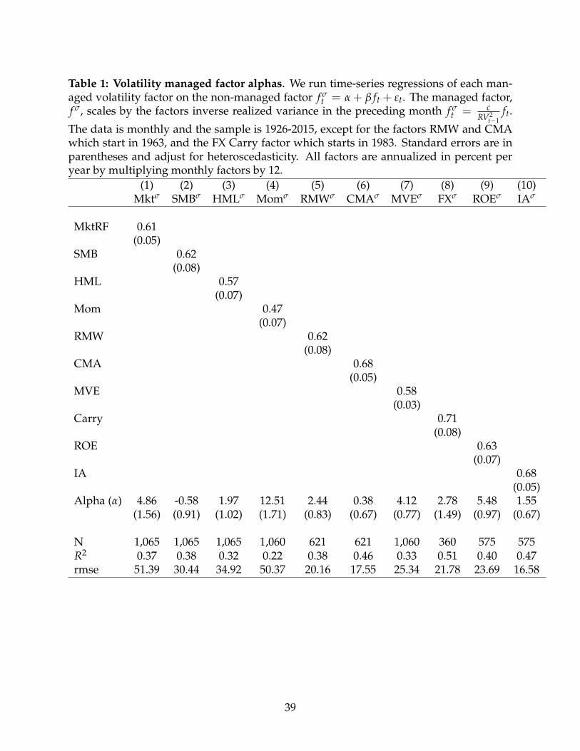
Table 1: Volatility managed factor alphas. We run time-series regressions of each man-aged volatility factor on the non-managed factor f σ

t = α + β ft + εt. The managed factor,f σ, scales by the factors inverse realized variance in the preceding month f σ

t = cRV2

t−1ft.

The data is monthly and the sample is 1926-2015, except for the factors RMW and CMAwhich start in 1963, and the FX Carry factor which starts in 1983. Standard errors are inparentheses and adjust for heteroscedasticity. All factors are annualized in percent peryear by multiplying monthly factors by 12.

(1) (2) (3) (4) (5) (6) (7) (8) (9) (10)Mktσ SMBσ HMLσ Momσ RMWσ CMAσ MVEσ FXσ ROEσ IAσ

MktRF 0.61(0.05)

SMB 0.62(0.08)

HML 0.57(0.07)

Mom 0.47(0.07)

RMW 0.62(0.08)

CMA 0.68(0.05)

MVE 0.58(0.03)

Carry 0.71(0.08)

ROE 0.63(0.07)

IA 0.68(0.05)

Alpha (α) 4.86 -0.58 1.97 12.51 2.44 0.38 4.12 2.78 5.48 1.55(1.56) (0.91) (1.02) (1.71) (0.83) (0.67) (0.77) (1.49) (0.97) (0.67)

N 1,065 1,065 1,065 1,060 621 621 1,060 360 575 575R2 0.37 0.38 0.32 0.22 0.38 0.46 0.33 0.51 0.40 0.47rmse 51.39 30.44 34.92 50.37 20.16 17.55 25.34 21.78 23.69 16.58

39

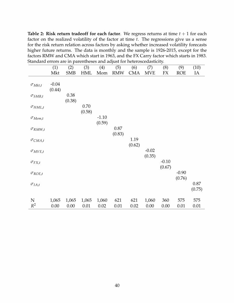
Table 2: Risk return tradeoff for each factor. We regress returns at time t + 1 for eachfactor on the realized volatility of the factor at time t. The regressions give us a sensefor the risk return relation across factors by asking whether increased volatility forecastshigher future returns. The data is monthly and the sample is 1926-2015, except for thefactors RMW and CMA which start in 1963, and the FX Carry factor which starts in 1983.Standard errors are in parentheses and adjust for heteroscedasticity.

(1) (2) (3) (4) (5) (6) (7) (8) (9) (10)Mkt SMB HML Mom RMW CMA MVE FX ROE IA

σMkt,t -0.04(0.44)

σSMB,t 0.38(0.38)

σHML,t 0.70(0.58)

σMom,t -1.10(0.59)

σRMW,t 0.87(0.83)

σCMA,t 1.19(0.62)

σMVE,t -0.02(0.35)

σFX,t -0.10(0.67)

σROE,t -0.90(0.76)

σIA,t 0.87(0.75)

N 1,065 1,065 1,065 1,060 621 621 1,060 360 575 575R2 0.00 0.00 0.01 0.02 0.01 0.02 0.00 0.00 0.01 0.01

40

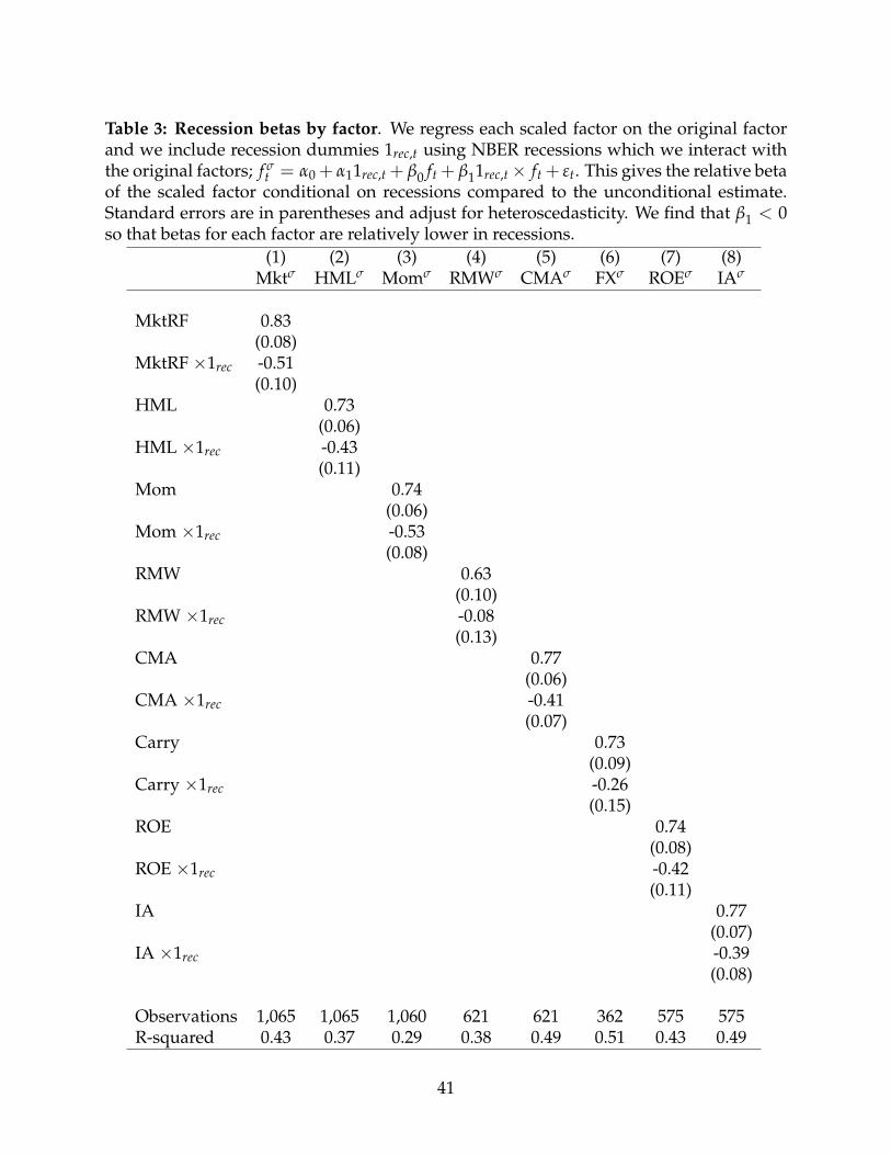
Table 3: Recession betas by factor. We regress each scaled factor on the original factorand we include recession dummies 1rec,t using NBER recessions which we interact withthe original factors; f σ

t = α0 + α11rec,t + β0 ft + β11rec,t× ft + εt. This gives the relative betaof the scaled factor conditional on recessions compared to the unconditional estimate.Standard errors are in parentheses and adjust for heteroscedasticity. We find that β1 < 0so that betas for each factor are relatively lower in recessions.

(1) (2) (3) (4) (5) (6) (7) (8)Mktσ HMLσ Momσ RMWσ CMAσ FXσ ROEσ IAσ

MktRF 0.83(0.08)

MktRF ×1rec -0.51(0.10)

HML 0.73(0.06)

HML ×1rec -0.43(0.11)

Mom 0.74(0.06)

Mom ×1rec -0.53(0.08)

RMW 0.63(0.10)

RMW ×1rec -0.08(0.13)

CMA 0.77(0.06)

CMA ×1rec -0.41(0.07)

Carry 0.73(0.09)

Carry ×1rec -0.26(0.15)

ROE 0.74(0.08)

ROE ×1rec -0.42(0.11)

IA 0.77(0.07)

IA ×1rec -0.39(0.08)

Observations 1,065 1,065 1,060 621 621 362 575 575R-squared 0.43 0.37 0.29 0.38 0.49 0.51 0.43 0.49

41

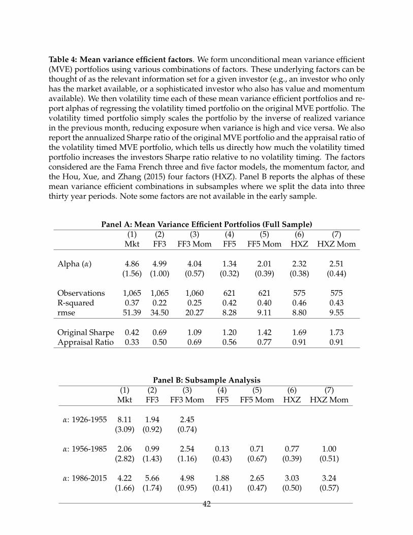
Table 4: Mean variance efficient factors. We form unconditional mean variance efficient(MVE) portfolios using various combinations of factors. These underlying factors can bethought of as the relevant information set for a given investor (e.g., an investor who onlyhas the market available, or a sophisticated investor who also has value and momentumavailable). We then volatility time each of these mean variance efficient portfolios and re-port alphas of regressing the volatility timed portfolio on the original MVE portfolio. Thevolatility timed portfolio simply scales the portfolio by the inverse of realized variancein the previous month, reducing exposure when variance is high and vice versa. We alsoreport the annualized Sharpe ratio of the original MVE portfolio and the appraisal ratio ofthe volatility timed MVE portfolio, which tells us directly how much the volatility timedportfolio increases the investors Sharpe ratio relative to no volatility timing. The factorsconsidered are the Fama French three and five factor models, the momentum factor, andthe Hou, Xue, and Zhang (2015) four factors (HXZ). Panel B reports the alphas of thesemean variance efficient combinations in subsamples where we split the data into threethirty year periods. Note some factors are not available in the early sample.

Panel A: Mean Variance Efficient Portfolios (Full Sample)(1) (2) (3) (4) (5) (6) (7)

Mkt FF3 FF3 Mom FF5 FF5 Mom HXZ HXZ Mom

Alpha (α) 4.86 4.99 4.04 1.34 2.01 2.32 2.51(1.56) (1.00) (0.57) (0.32) (0.39) (0.38) (0.44)

Observations 1,065 1,065 1,060 621 621 575 575R-squared 0.37 0.22 0.25 0.42 0.40 0.46 0.43rmse 51.39 34.50 20.27 8.28 9.11 8.80 9.55

Original Sharpe 0.42 0.69 1.09 1.20 1.42 1.69 1.73Appraisal Ratio 0.33 0.50 0.69 0.56 0.77 0.91 0.91

Panel B: Subsample Analysis(1) (2) (3) (4) (5) (6) (7)

Mkt FF3 FF3 Mom FF5 FF5 Mom HXZ HXZ Mom

α: 1926-1955 8.11 1.94 2.45(3.09) (0.92) (0.74)

α: 1956-1985 2.06 0.99 2.54 0.13 0.71 0.77 1.00(2.82) (1.43) (1.16) (0.43) (0.67) (0.39) (0.51)

α: 1986-2015 4.22 5.66 4.98 1.88 2.65 3.03 3.24(1.66) (1.74) (0.95) (0.41) (0.47) (0.50) (0.57)

42

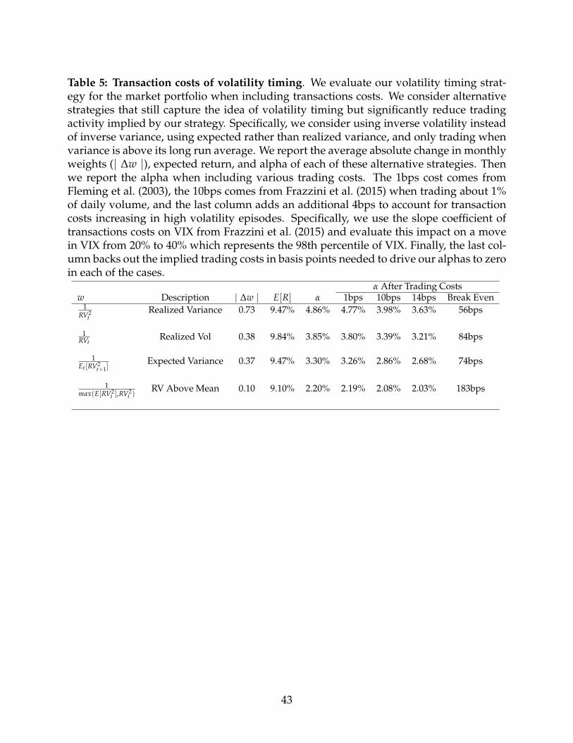
Table 5: Transaction costs of volatility timing. We evaluate our volatility timing strat-egy for the market portfolio when including transactions costs. We consider alternativestrategies that still capture the idea of volatility timing but significantly reduce tradingactivity implied by our strategy. Specifically, we consider using inverse volatility insteadof inverse variance, using expected rather than realized variance, and only trading whenvariance is above its long run average. We report the average absolute change in monthlyweights (| ∆w |), expected return, and alpha of each of these alternative strategies. Thenwe report the alpha when including various trading costs. The 1bps cost comes fromFleming et al. (2003), the 10bps comes from Frazzini et al. (2015) when trading about 1%of daily volume, and the last column adds an additional 4bps to account for transactioncosts increasing in high volatility episodes. Specifically, we use the slope coefficient oftransactions costs on VIX from Frazzini et al. (2015) and evaluate this impact on a movein VIX from 20% to 40% which represents the 98th percentile of VIX. Finally, the last col-umn backs out the implied trading costs in basis points needed to drive our alphas to zeroin each of the cases.

α After Trading Costsw Description | ∆w | E[R] α 1bps 10bps 14bps Break Even

1RV2

tRealized Variance 0.73 9.47% 4.86% 4.77% 3.98% 3.63% 56bps

1RVt

Realized Vol 0.38 9.84% 3.85% 3.80% 3.39% 3.21% 84bps

1Et [RV2

t+1]Expected Variance 0.37 9.47% 3.30% 3.26% 2.86% 2.68% 74bps

1max(E[RV2

t ],RV2t )

RV Above Mean 0.10 9.10% 2.20% 2.19% 2.08% 2.03% 183bps

43

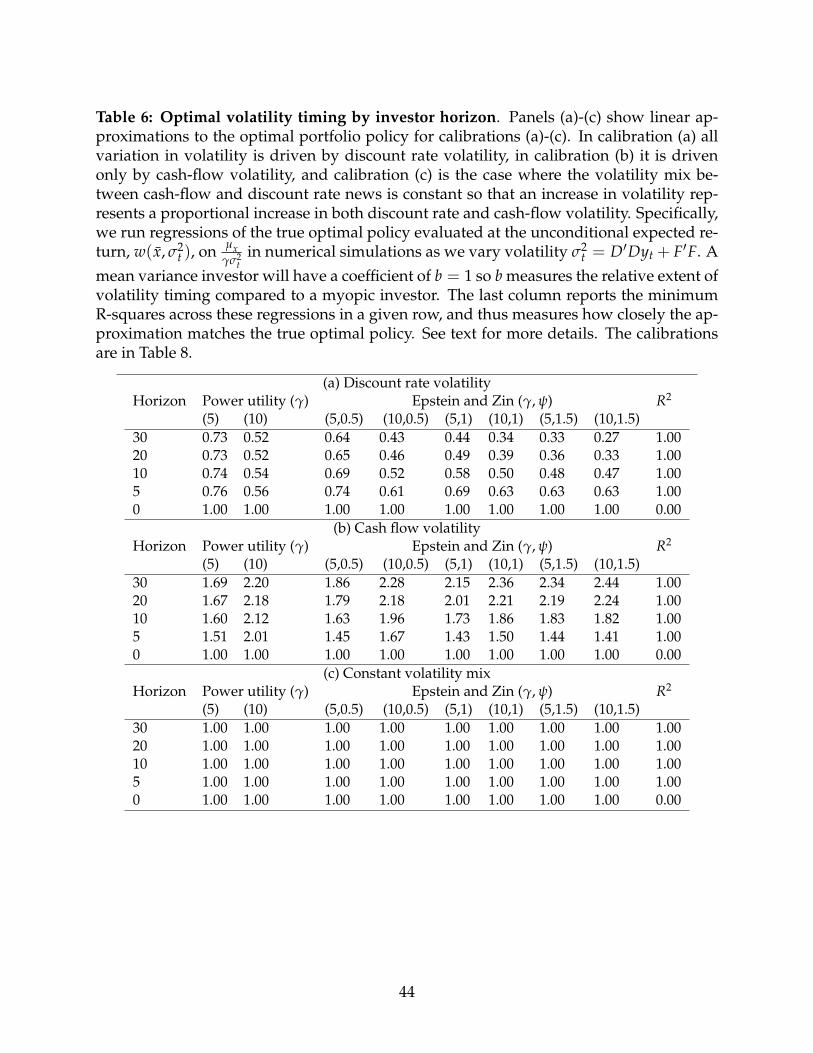
Table 6: Optimal volatility timing by investor horizon. Panels (a)-(c) show linear ap-proximations to the optimal portfolio policy for calibrations (a)-(c). In calibration (a) allvariation in volatility is driven by discount rate volatility, in calibration (b) it is drivenonly by cash-flow volatility, and calibration (c) is the case where the volatility mix be-tween cash-flow and discount rate news is constant so that an increase in volatility rep-resents a proportional increase in both discount rate and cash-flow volatility. Specifically,we run regressions of the true optimal policy evaluated at the unconditional expected re-turn, w(x, σ2

t ), on µxγσ2

tin numerical simulations as we vary volatility σ2

t = D′Dyt + F′F. Amean variance investor will have a coefficient of b = 1 so b measures the relative extent ofvolatility timing compared to a myopic investor. The last column reports the minimumR-squares across these regressions in a given row, and thus measures how closely the ap-proximation matches the true optimal policy. See text for more details. The calibrationsare in Table 8.

(a) Discount rate volatilityHorizon Power utility (γ) Epstein and Zin (γ, ψ) R2

(5) (10) (5,0.5) (10,0.5) (5,1) (10,1) (5,1.5) (10,1.5)30 0.73 0.52 0.64 0.43 0.44 0.34 0.33 0.27 1.0020 0.73 0.52 0.65 0.46 0.49 0.39 0.36 0.33 1.0010 0.74 0.54 0.69 0.52 0.58 0.50 0.48 0.47 1.005 0.76 0.56 0.74 0.61 0.69 0.63 0.63 0.63 1.000 1.00 1.00 1.00 1.00 1.00 1.00 1.00 1.00 0.00

(b) Cash flow volatilityHorizon Power utility (γ) Epstein and Zin (γ, ψ) R2

(5) (10) (5,0.5) (10,0.5) (5,1) (10,1) (5,1.5) (10,1.5)30 1.69 2.20 1.86 2.28 2.15 2.36 2.34 2.44 1.0020 1.67 2.18 1.79 2.18 2.01 2.21 2.19 2.24 1.0010 1.60 2.12 1.63 1.96 1.73 1.86 1.83 1.82 1.005 1.51 2.01 1.45 1.67 1.43 1.50 1.44 1.41 1.000 1.00 1.00 1.00 1.00 1.00 1.00 1.00 1.00 0.00

(c) Constant volatility mixHorizon Power utility (γ) Epstein and Zin (γ, ψ) R2

(5) (10) (5,0.5) (10,0.5) (5,1) (10,1) (5,1.5) (10,1.5)30 1.00 1.00 1.00 1.00 1.00 1.00 1.00 1.00 1.0020 1.00 1.00 1.00 1.00 1.00 1.00 1.00 1.00 1.0010 1.00 1.00 1.00 1.00 1.00 1.00 1.00 1.00 1.005 1.00 1.00 1.00 1.00 1.00 1.00 1.00 1.00 1.000 1.00 1.00 1.00 1.00 1.00 1.00 1.00 1.00 0.00

44

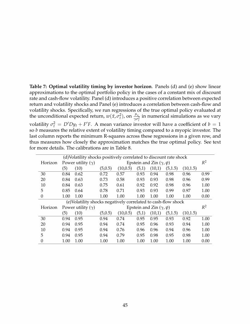
Table 7: Optimal volatility timing by investor horizon. Panels (d) and (e) show linearapproximations to the optimal portfolio policy in the cases of a constant mix of discountrate and cash-flow volatility. Panel (d) introduces a positive correlation between expectedreturn and volatility shocks and Panel (e) introduces a correlation between cash-flow andvolatility shocks. Specifically, we run regressions of the true optimal policy evaluated atthe unconditional expected return, w(x, σ2

t ), on µxγσ2

tin numerical simulations as we vary

volatility σ2t = D′Dyt + F′F. A mean variance investor will have a coefficient of b = 1

so b measures the relative extent of volatility timing compared to a myopic investor. Thelast column reports the minimum R-squares across these regressions in a given row, andthus measures how closely the approximation matches the true optimal policy. See textfor more details. The calibrations are in Table 8.

(d)Volatility shocks positively correlated to discount rate shockHorizon Power utility (γ) Epstein and Zin (γ, ψ) R2

(5) (10) (5,0.5) (10,0.5) (5,1) (10,1) (5,1.5) (10,1.5)30 0.84 0.62 0.72 0.57 0.93 0.94 0.98 0.96 0.9920 0.84 0.63 0.73 0.58 0.93 0.93 0.98 0.96 0.9910 0.84 0.63 0.75 0.61 0.92 0.92 0.98 0.96 1.005 0.85 0.64 0.78 0.71 0.93 0.93 0.99 0.97 1.000 1.00 1.00 1.00 1.00 1.00 1.00 1.00 1.00 0.00

(e)Volatility shocks negatively correlated to cash-flow shockHorizon Power utility (γ) Epstein and Zin (γ, ψ) R2

(5) (10) (5,0.5) (10,0.5) (5,1) (10,1) (5,1.5) (10,1.5)30 0.94 0.95 0.94 0.74 0.95 0.95 0.93 0.92 1.0020 0.94 0.95 0.94 0.74 0.95 0.96 0.93 0.94 1.0010 0.94 0.95 0.94 0.76 0.96 0.96 0.94 0.96 1.005 0.94 0.95 0.94 0.79 0.95 0.98 0.95 0.98 1.000 1.00 1.00 1.00 1.00 1.00 1.00 1.00 1.00 0.00

45

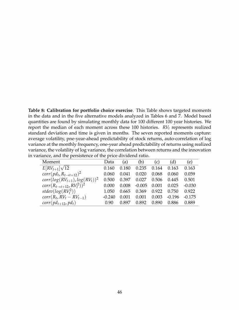
Table 8: Calibration for portfolio choice exercise. This Table shows targeted momentsin the data and in the five alternative models analyzed in Tables 6 and 7. Model basedquantities are found by simulating monthly data for 100 different 100 year histories. Wereport the median of each moment across these 100 histories. RVt represents realizedstandard deviation and time is given in months. The seven reported moments capture:average volatility, pne-year-ahead predictability of stock returns, auto-correlation of logvariance at the monthly frequency, one-year ahead predictability of returns using realizedvariance, the volatility of log variance, the correlation between returns and the innovationin variance, and the persistence of the price dividend ratio.

Moment Data (a) (b) (c) (d) (e)E[RVt+1]

√12 0.160 0.180 0.235 0.164 0.163 0.163

corr(pdt, Rt→t+12)2 0.060 0.041 0.020 0.068 0.060 0.059

corr(log(RVt+1), log(RVt))2 0.500 0.397 0.027 0.506 0.445 0.501corr(Rt→t+12, RV2

t ))2 0.000 0.008 -0.005 0.001 0.025 -0.030

stdev(log(RV2t )) 1.050 0.665 0.369 0.922 0.750 0.922

corr(Rt, RVt − RVt−1) -0.240 0.001 0.001 0.003 -0.196 -0.175corr(pdt+12, pdt) 0.90 0.897 0.892 0.890 0.886 0.889

46

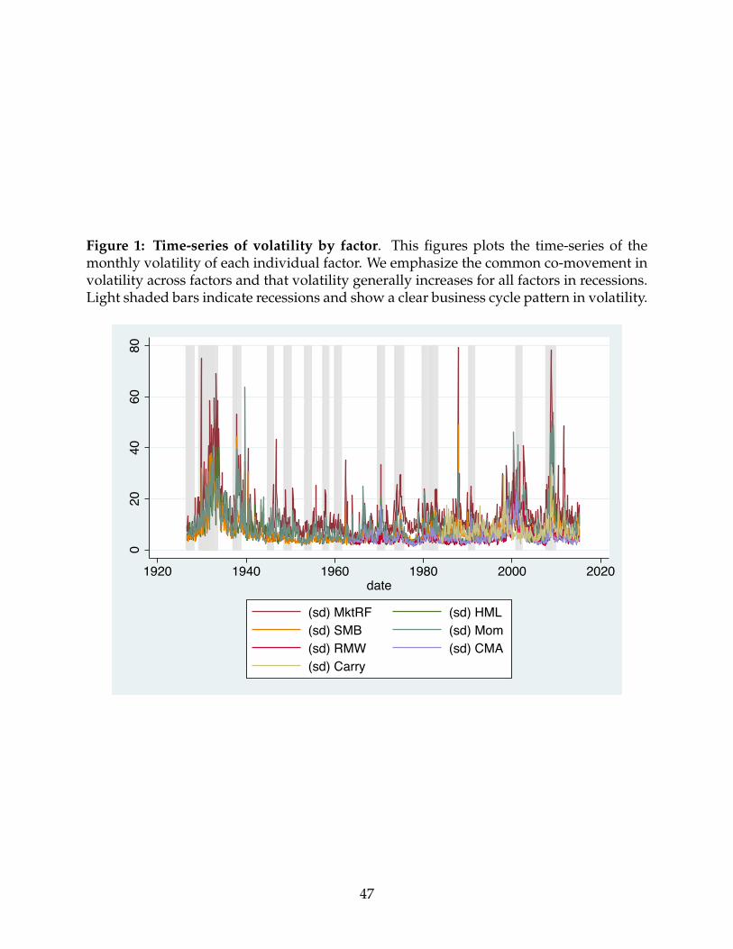
Figure 1: Time-series of volatility by factor. This figures plots the time-series of themonthly volatility of each individual factor. We emphasize the common co-movement involatility across factors and that volatility generally increases for all factors in recessions.Light shaded bars indicate recessions and show a clear business cycle pattern in volatility.

020

4060

80

1920 1940 1960 1980 2000 2020date

(sd) MktRF (sd) HML(sd) SMB (sd) Mom(sd) RMW (sd) CMA(sd) Carry

47

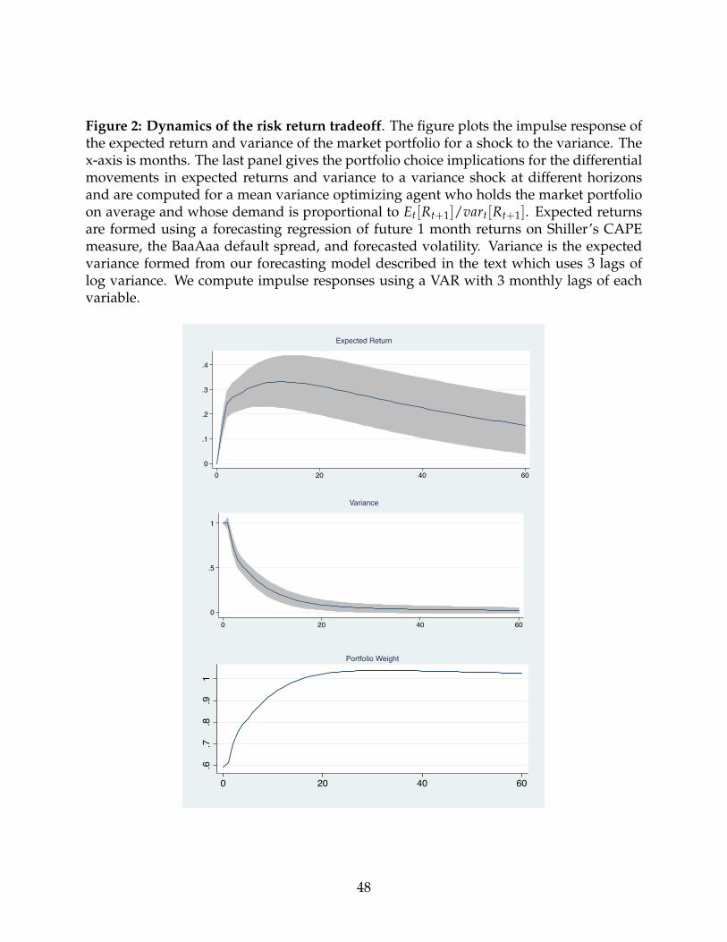
Figure 2: Dynamics of the risk return tradeoff. The figure plots the impulse response ofthe expected return and variance of the market portfolio for a shock to the variance. Thex-axis is months. The last panel gives the portfolio choice implications for the differentialmovements in expected returns and variance to a variance shock at different horizonsand are computed for a mean variance optimizing agent who holds the market portfolioon average and whose demand is proportional to Et[Rt+1]/vart[Rt+1]. Expected returnsare formed using a forecasting regression of future 1 month returns on Shiller’s CAPEmeasure, the BaaAaa default spread, and forecasted volatility. Variance is the expectedvariance formed from our forecasting model described in the text which uses 3 lags oflog variance. We compute impulse responses using a VAR with 3 monthly lags of eachvariable.

0

.1

.2

.3

.4

0 20 40 60

Expected Return

0

.5

1

0 20 40 60

Variance

.6.7

.8.9

1

0 20 40 60

Portfolio Weight

48

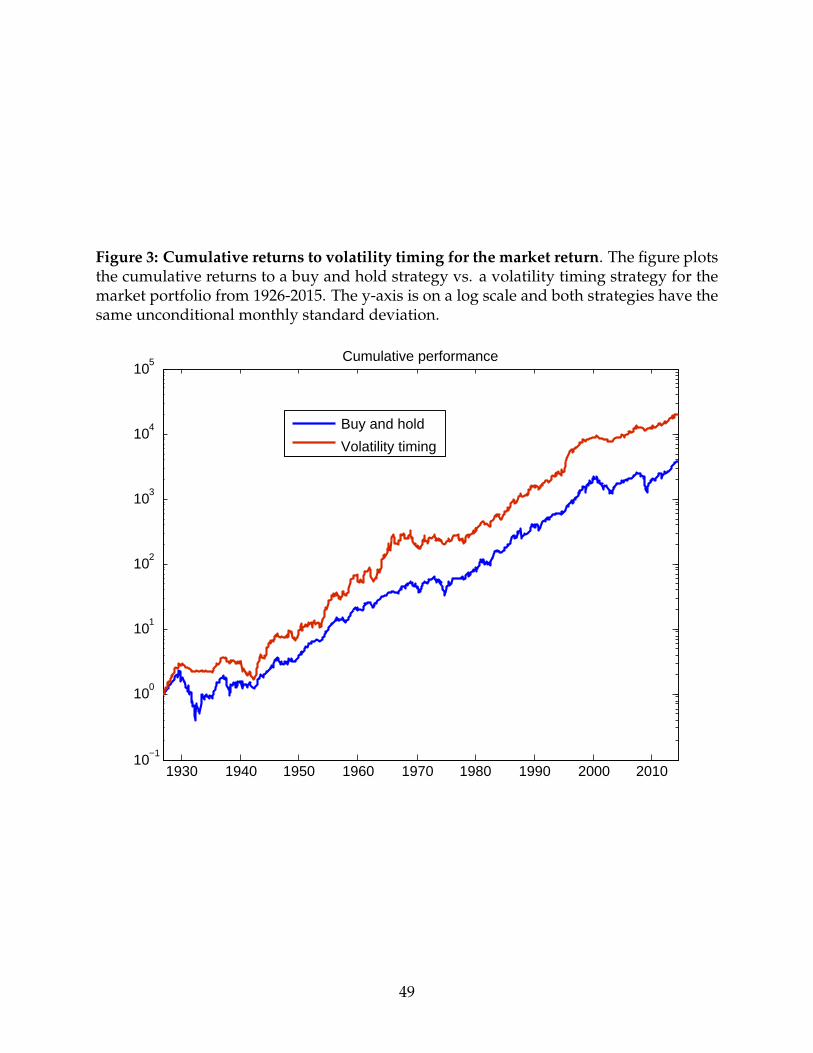
Figure 3: Cumulative returns to volatility timing for the market return. The figure plotsthe cumulative returns to a buy and hold strategy vs. a volatility timing strategy for themarket portfolio from 1926-2015. The y-axis is on a log scale and both strategies have thesame unconditional monthly standard deviation.

1930 1940 1950 1960 1970 1980 1990 2000 201010

−1

100

101

102

103

104

105 Cumulative performance

Buy and hold

Volatility timing

49

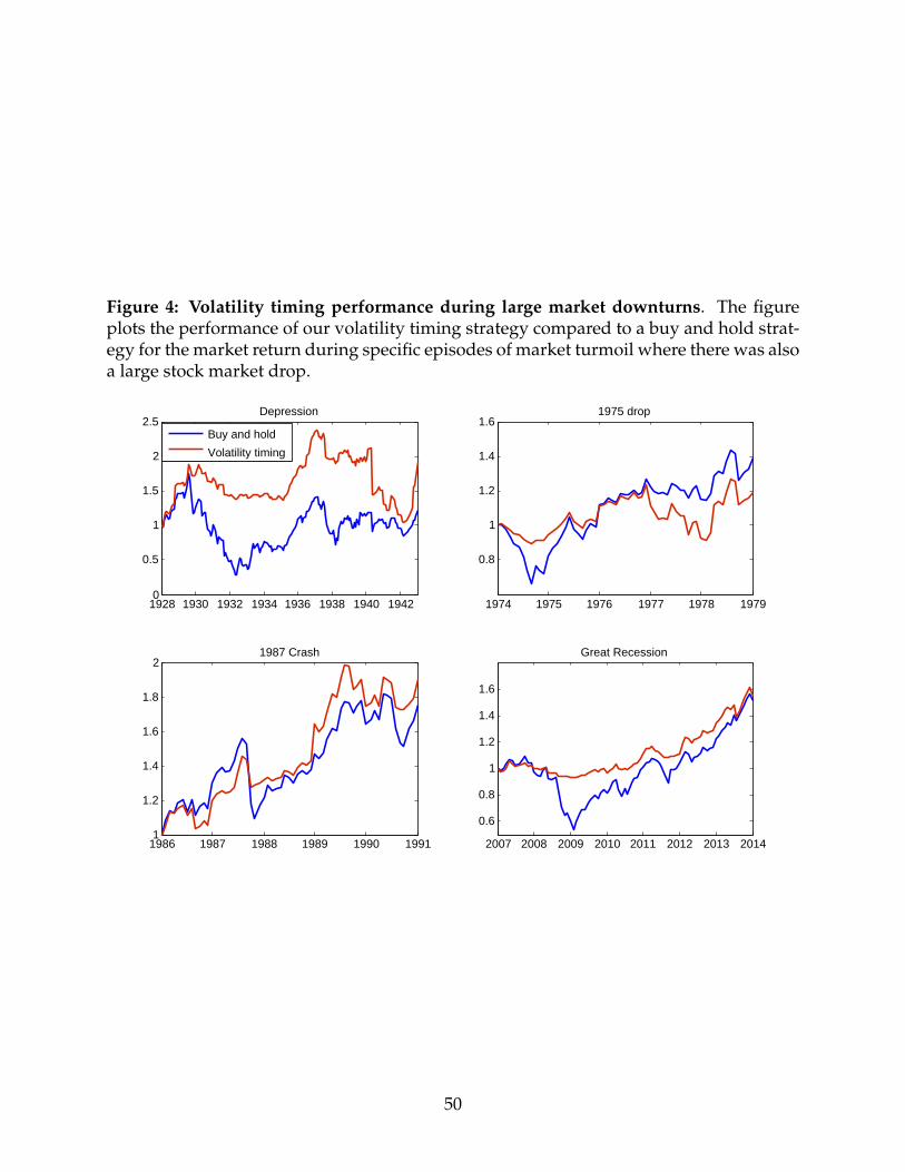
Figure 4: Volatility timing performance during large market downturns. The figureplots the performance of our volatility timing strategy compared to a buy and hold strat-egy for the market return during specific episodes of market turmoil where there was alsoa large stock market drop.

1928 1930 1932 1934 1936 1938 1940 19420

0.5

1

1.5

2

2.5Depression

Buy and hold

Volatility timing

1974 1975 1976 1977 1978 1979

0.8

1

1.2

1.4

1.61975 drop

1986 1987 1988 1989 1990 19911

1.2

1.4

1.6

1.8

21987 Crash

2007 2008 2009 2010 2011 2012 2013 2014

0.6

0.8

1

1.2

1.4

1.6

Great Recession

50

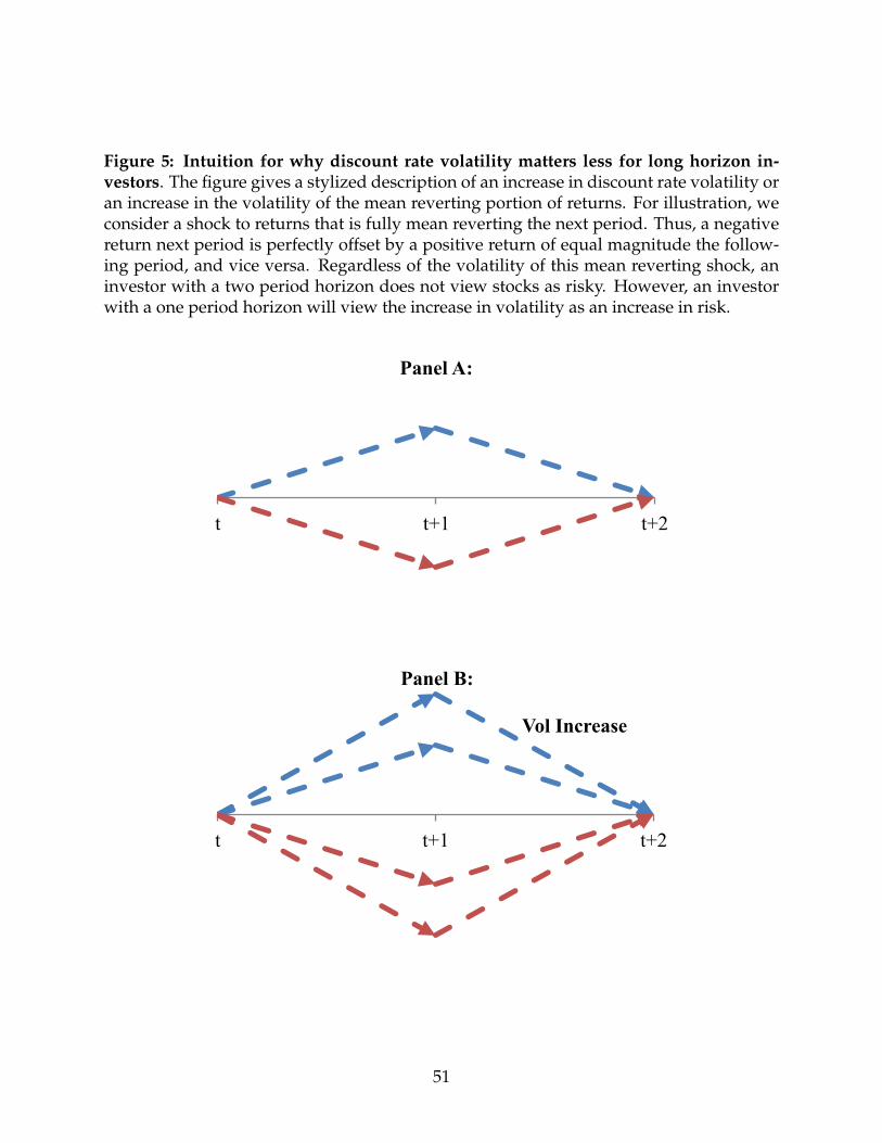
Figure 5: Intuition for why discount rate volatility matters less for long horizon in-vestors. The figure gives a stylized description of an increase in discount rate volatility oran increase in the volatility of the mean reverting portion of returns. For illustration, weconsider a shock to returns that is fully mean reverting the next period. Thus, a negativereturn next period is perfectly offset by a positive return of equal magnitude the follow-ing period, and vice versa. Regardless of the volatility of this mean reverting shock, aninvestor with a two period horizon does not view stocks as risky. However, an investorwith a one period horizon will view the increase in volatility as an increase in risk.

t t+1 t+2

Panel A:

t t+1 t+2

Panel B:

Vol Increase

51

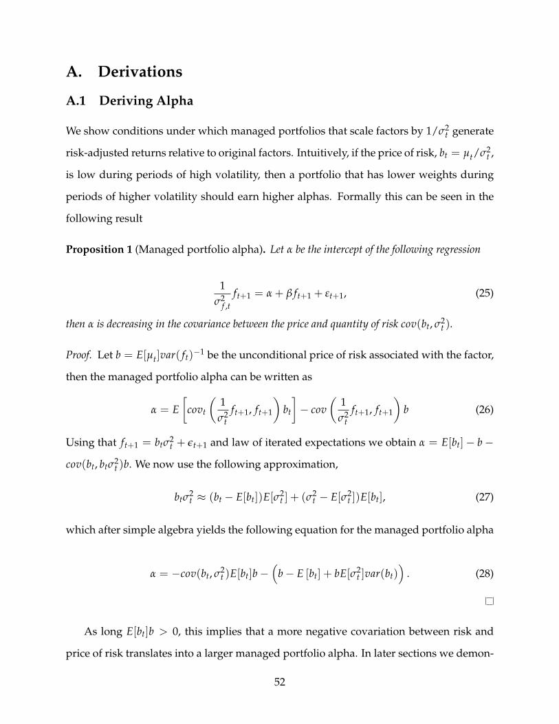
A. Derivations

A.1 Deriving Alpha

We show conditions under which managed portfolios that scale factors by 1/σ2t generate

risk-adjusted returns relative to original factors. Intuitively, if the price of risk, bt = µt/σ2t ,

is low during periods of high volatility, then a portfolio that has lower weights during

periods of higher volatility should earn higher alphas. Formally this can be seen in the

following result

Proposition 1 (Managed portfolio alpha). Let α be the intercept of the following regression

1σ2

f ,tft+1 = α + β ft+1 + εt+1, (25)

then α is decreasing in the covariance between the price and quantity of risk cov(bt, σ2t ).

Proof. Let b = E[µt]var( ft)−1 be the unconditional price of risk associated with the factor,

then the managed portfolio alpha can be written as

α = E[

covt

(1σ2

tft+1, ft+1

)bt

]− cov

(1σ2

tft+1, ft+1

)b (26)

Using that ft+1 = btσ2t + εt+1 and law of iterated expectations we obtain α = E[bt]− b−

cov(bt, btσ2t )b. We now use the following approximation,

btσ2t ≈ (bt − E[bt])E[σ2

t ] + (σ2t − E[σ2

t ])E[bt], (27)

which after simple algebra yields the following equation for the managed portfolio alpha

α = −cov(bt, σ2t )E[bt]b−

(b− E [bt] + bE[σ2

t ]var(bt))

. (28)

As long E[bt]b > 0, this implies that a more negative covariation between risk and

price of risk translates into a larger managed portfolio alpha. In later sections we demon-

52

strate that indeed the covariance is negative. This stems from the simple fact that volatil-

ity does not strongly forecast returns. The next section derives this covariance term more

carefully.

A.2 Derivation of Equation Covariance

Let ft+1 be the excess return on the factor. Let µt denote the conditional expected return

on the factor, Et[ ft+1], and σ2t denote the conditional variance, vart[ ft+1]. It is useful to

keep in mind the equation

µt = btσ2t (29)

The coefficient in the regression of future realized excess return ft+1 on past inverse

volatility is

β =cov( ft+1, −1

σ2t)

var( 1σ2

t)

(30)

We can replace ft+1 with ft+1 = µt + εt+1 in the above equation. Note that the error

term εt+1 will have zero covariance with any time t variable. Next replace µt = btσ2t so

that we have

β =cov(btσ

2t , 1

σ2t)

var( 1σ2

t)

(31)

Next, we make use of the following identity in order to simplify the numerator above:

cov(xy, z) = cov (x, y(z− E[z])) + E[x]cov(y, z) (32)

This means

β =

[cov(bt, σ2

t (E[1/σ2t ] + cov(σ2

t , 1/σ2t )/E[σ2

t ]))−µ

E[σ2t ]

cov(σ2t , 1/σ2

t )

]/var(1/σ2

t )

(33)

But then

cov(σ2t , 1/σ2

t ) = 1− E[σ2t ]E[1/σ2

t ] (34)

53

So that

β =

[cov(bt, σ2

t )/E[σ2t ] +

µ

E[σ2t ](E[σ2

t ]E[1/σ2t ]− 1)

]/var(1/σ2

t ) (35)

Rearranging,

cov(bt, σ2t ) = E[σ2

t ]var(1/σ2t )

(β− µ

E[σ2t ]

(E[σ2t ]E[1/σ2

t ]− 1)var(1/σ2

t )

)(36)

We can thus estimate this co-variance. First, we could run the regression of returns

on negative inverse variance then compute all other quantities. We find the co-variance

to be strongly negative for almost all factors. This means the alpha shown in the previous

section is typically going to be positive.

54

B. Additional Figures

55

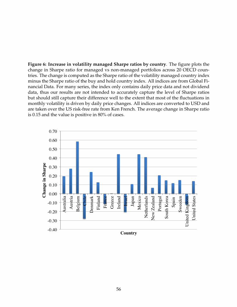
Figure 6: Increase in volatility managed Sharpe ratios by country. The figure plots thechange in Sharpe ratio for managed vs non-managed portfolios across 20 OECD coun-tries. The change is computed as the Sharpe ratio of the volatility managed country indexminus the Sharpe ratio of the buy and hold country index. All indices are from Global Fi-nancial Data. For many series, the index only contains daily price data and not dividenddata, thus our results are not intended to accurately capture the level of Sharpe ratiosbut should still capture their difference well to the extent that most of the fluctuations inmonthly volatility is driven by daily price changes. All indices are converted to USD andare taken over the US risk-free rate from Ken French. The average change in Sharpe ratiois 0.15 and the value is positive in 80% of cases.

-0.40

-0.30

-0.20

-0.10

0.00

0.10

0.20

0.30

0.40

0.50

0.60

0.70

Aus

tralia

Aus

tria

Belg

ium

Chile

Den

mar

kFi

nlan

dFr

ance

Gre

ece

Irela

ndIs

rael

Japa

nM

exic

oN

ethe

rland

sN

ew Z

eala

ndPo

rtuga

lSo

uth

Kor

eaSp

ain

Swee

den

Uni

ted

Kin

gdom

Uni

ted

Stat

esCha

nge

in S

harp

e

Country

56

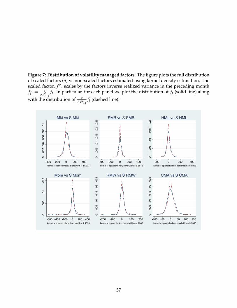
Figure 7: Distribution of volatility managed factors. The figure plots the full distributionof scaled factors (S) vs non-scaled factors estimated using kernel density estimation. Thescaled factor, f σ, scales by the factors inverse realized variance in the preceding monthf σt = c

RV2t−1

ft. In particular, for each panel we plot the distribution of ft (solid line) along

with the distribution of cRV2

t−1ft (dashed line).

0.0

02.0

04.0

06.0

08.0

1

-400 -200 0 200 400kernel = epanechnikov, bandwidth = 11.2774

Mkt vs S Mkt

0.0

05.0

1.0

15.0

2.0

25

-400 -200 0 200 400kernel = epanechnikov, bandwidth = 6.6513

SMB vs S SMB

0.0

05.0

1.0

15.0

2

-200 0 200 400kernel = epanechnikov, bandwidth = 6.0358

HML vs S HML

0.0

05.0

1.0

15

-600 -400 -200 0 200 400kernel = epanechnikov, bandwidth = 7.4539

Mom vs S Mom

0.0

05.0

1.0

15.0

2.0

25

-200 -100 0 100 200kernel = epanechnikov, bandwidth = 4.7986

RMW vs S RMW

0.0

05.0

1.0

15.0

2.0

25

-100 -50 0 50 100 150kernel = epanechnikov, bandwidth = 5.3956

CMA vs S CMA

57

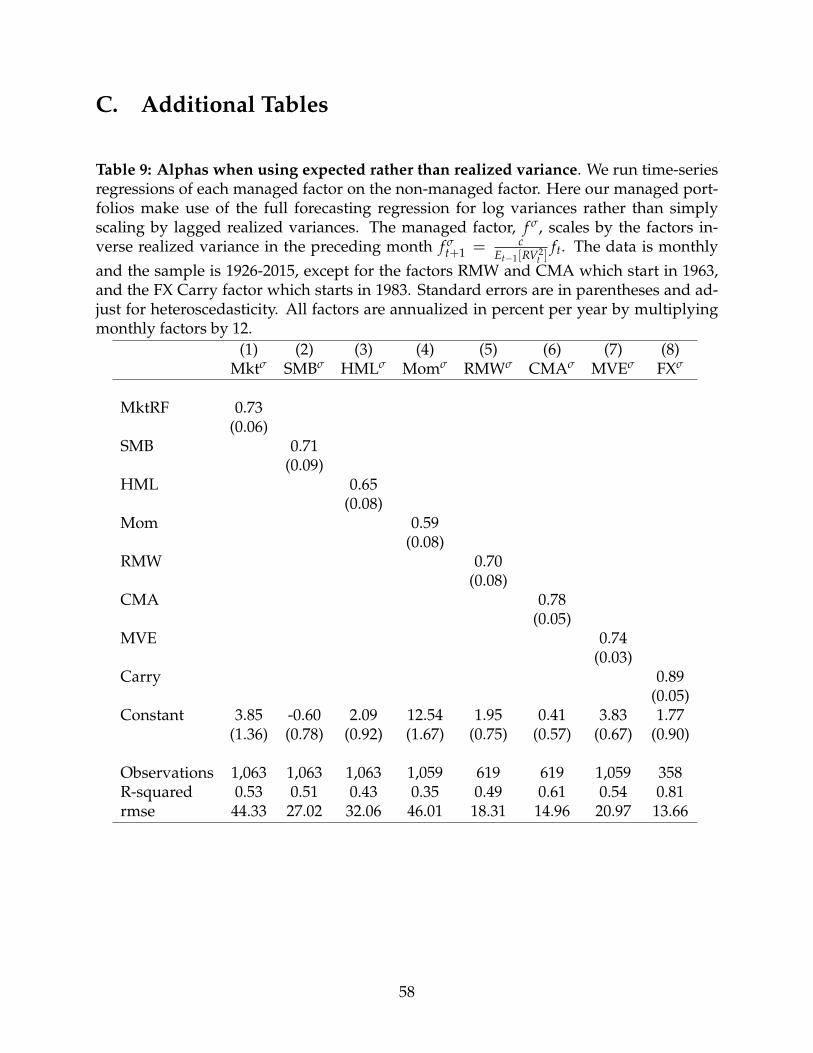
C. Additional Tables

Table 9: Alphas when using expected rather than realized variance. We run time-seriesregressions of each managed factor on the non-managed factor. Here our managed port-folios make use of the full forecasting regression for log variances rather than simplyscaling by lagged realized variances. The managed factor, f σ, scales by the factors in-verse realized variance in the preceding month f σ

t+1 = cEt−1[RV2

t ]ft. The data is monthly

and the sample is 1926-2015, except for the factors RMW and CMA which start in 1963,and the FX Carry factor which starts in 1983. Standard errors are in parentheses and ad-just for heteroscedasticity. All factors are annualized in percent per year by multiplyingmonthly factors by 12.

(1) (2) (3) (4) (5) (6) (7) (8)Mktσ SMBσ HMLσ Momσ RMWσ CMAσ MVEσ FXσ

MktRF 0.73(0.06)

SMB 0.71(0.09)

HML 0.65(0.08)

Mom 0.59(0.08)

RMW 0.70(0.08)

CMA 0.78(0.05)

MVE 0.74(0.03)

Carry 0.89(0.05)

Constant 3.85 -0.60 2.09 12.54 1.95 0.41 3.83 1.77(1.36) (0.78) (0.92) (1.67) (0.75) (0.57) (0.67) (0.90)

Observations 1,063 1,063 1,063 1,059 619 619 1,059 358R-squared 0.53 0.51 0.43 0.35 0.49 0.61 0.54 0.81rmse 44.33 27.02 32.06 46.01 18.31 14.96 20.97 13.66

58

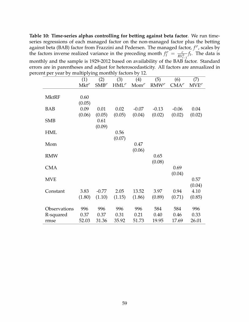
Table 10: Time-series alphas controlling for betting against beta factor. We run time-series regressions of each managed factor on the non-managed factor plus the bettingagainst beta (BAB) factor from Frazzini and Pedersen. The managed factor, f σ, scales bythe factors inverse realized variance in the preceding month f σ

t = cRV2

t−1ft. The data is

monthly and the sample is 1929-2012 based on availability of the BAB factor. Standarderrors are in parentheses and adjust for heteroscedasticity. All factors are annualized inpercent per year by multiplying monthly factors by 12.

(1) (2) (3) (4) (5) (6) (7)Mktσ SMBσ HMLσ Momσ RMWσ CMAσ MVEσ

MktRF 0.60(0.05)

BAB 0.09 0.01 0.02 -0.07 -0.13 -0.06 0.04(0.06) (0.05) (0.05) (0.04) (0.02) (0.02) (0.02)

SMB 0.61(0.09)

HML 0.56(0.07)

Mom 0.47(0.06)

RMW 0.65(0.08)

CMA 0.69(0.04)

MVE 0.57(0.04)

Constant 3.83 -0.77 2.05 13.52 3.97 0.94 4.10(1.80) (1.10) (1.15) (1.86) (0.89) (0.71) (0.85)

Observations 996 996 996 996 584 584 996R-squared 0.37 0.37 0.31 0.21 0.40 0.46 0.33rmse 52.03 31.36 35.92 51.73 19.95 17.69 26.01

59

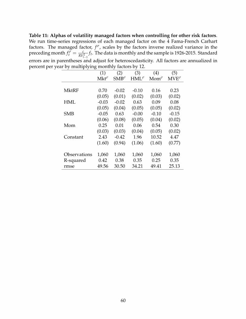
Table 11: Alphas of volatility managed factors when controlling for other risk factors.We run time-series regressions of each managed factor on the 4 Fama-French Carhartfactors. The managed factor, f σ, scales by the factors inverse realized variance in thepreceding month f σ

t = cRV2

t−1ft. The data is monthly and the sample is 1926-2015. Standard

errors are in parentheses and adjust for heteroscedasticity. All factors are annualized inpercent per year by multiplying monthly factors by 12.

(1) (2) (3) (4) (5)Mktσ SMBσ HMLσ Momσ MVEσ

MktRF 0.70 -0.02 -0.10 0.16 0.23(0.05) (0.01) (0.02) (0.03) (0.02)

HML -0.03 -0.02 0.63 0.09 0.08(0.05) (0.04) (0.05) (0.05) (0.02)

SMB -0.05 0.63 -0.00 -0.10 -0.15(0.06) (0.08) (0.05) (0.04) (0.02)

Mom 0.25 0.01 0.06 0.54 0.30(0.03) (0.03) (0.04) (0.05) (0.02)

Constant 2.43 -0.42 1.96 10.52 4.47(1.60) (0.94) (1.06) (1.60) (0.77)

Observations 1,060 1,060 1,060 1,060 1,060R-squared 0.42 0.38 0.35 0.25 0.35rmse 49.56 30.50 34.21 49.41 25.13

60

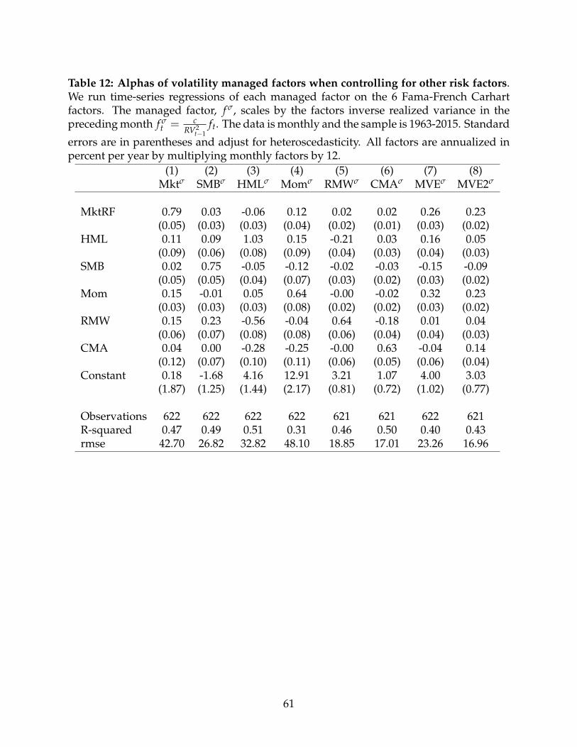
Table 12: Alphas of volatility managed factors when controlling for other risk factors.We run time-series regressions of each managed factor on the 6 Fama-French Carhartfactors. The managed factor, f σ, scales by the factors inverse realized variance in thepreceding month f σ

t = cRV2

t−1ft. The data is monthly and the sample is 1963-2015. Standard

errors are in parentheses and adjust for heteroscedasticity. All factors are annualized inpercent per year by multiplying monthly factors by 12.

(1) (2) (3) (4) (5) (6) (7) (8)Mktσ SMBσ HMLσ Momσ RMWσ CMAσ MVEσ MVE2σ

MktRF 0.79 0.03 -0.06 0.12 0.02 0.02 0.26 0.23(0.05) (0.03) (0.03) (0.04) (0.02) (0.01) (0.03) (0.02)

HML 0.11 0.09 1.03 0.15 -0.21 0.03 0.16 0.05(0.09) (0.06) (0.08) (0.09) (0.04) (0.03) (0.04) (0.03)

SMB 0.02 0.75 -0.05 -0.12 -0.02 -0.03 -0.15 -0.09(0.05) (0.05) (0.04) (0.07) (0.03) (0.02) (0.03) (0.02)

Mom 0.15 -0.01 0.05 0.64 -0.00 -0.02 0.32 0.23(0.03) (0.03) (0.03) (0.08) (0.02) (0.02) (0.03) (0.02)

RMW 0.15 0.23 -0.56 -0.04 0.64 -0.18 0.01 0.04(0.06) (0.07) (0.08) (0.08) (0.06) (0.04) (0.04) (0.03)

CMA 0.04 0.00 -0.28 -0.25 -0.00 0.63 -0.04 0.14(0.12) (0.07) (0.10) (0.11) (0.06) (0.05) (0.06) (0.04)

Constant 0.18 -1.68 4.16 12.91 3.21 1.07 4.00 3.03(1.87) (1.25) (1.44) (2.17) (0.81) (0.72) (1.02) (0.77)

Observations 622 622 622 622 621 621 622 621R-squared 0.47 0.49 0.51 0.31 0.46 0.50 0.40 0.43rmse 42.70 26.82 32.82 48.10 18.85 17.01 23.26 16.96

61

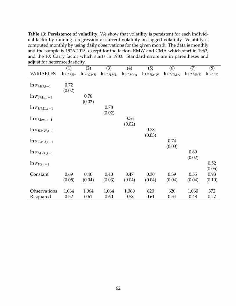
Table 13: Persistence of volatility. We show that volatility is persistent for each individ-ual factor by running a regression of current volatility on lagged volatility. Volatility iscomputed monthly by using daily observations for the given month. The data is monthlyand the sample is 1926-2015, except for the factors RMW and CMA which start in 1963,and the FX Carry factor which starts in 1983. Standard errors are in parentheses andadjust for heteroscedasticity.

(1) (2) (3) (4) (5) (6) (7) (8)VARIABLES ln σMkt ln σSMB ln σHML ln σMom ln σRMW ln σCMA ln σMVE ln σFX

ln σMkt,t−1 0.72(0.02)

ln σSMB,t−1 0.78(0.02)

ln σHML,t−1 0.78(0.02)

ln σMom,t−1 0.76(0.02)

ln σRMW,t−1 0.78(0.03)

ln σCMA,t−1 0.74(0.03)

ln σMVE,t−1 0.69(0.02)

ln σFX,t−1 0.52(0.05)

Constant 0.69 0.40 0.40 0.47 0.30 0.39 0.55 0.93(0.05) (0.04) (0.03) (0.04) (0.04) (0.04) (0.04) (0.10)

Observations 1,064 1,064 1,064 1,060 620 620 1,060 372R-squared 0.52 0.61 0.60 0.58 0.61 0.54 0.48 0.27

62

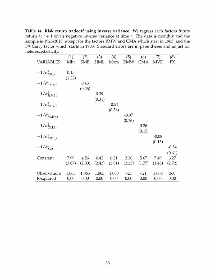
Table 14: Risk return tradeoff using inverse variance. We regress each factors futurereturn at t + 1 on its negative inverse variance at time t. The data is monthly and thesample is 1926-2015, except for the factors RMW and CMA which start in 1963, and theFX Carry factor which starts in 1983. Standard errors are in parentheses and adjust forheteroscedasticity.

(1) (2) (3) (4) (5) (6) (7) (8)VARIABLES Mkt SMB HML Mom RMW CMA MVE FX

−1/σ2Mkt,t 0.15

(1.22)−1/σ2

SMB,t 0.45(0.26)

−1/σ2HML,t 0.39

(0.31)−1/σ2

Mom,t -0.51(0.36)

−1/σ2RMW,t -0.07

(0.16)−1/σ2

CMA,t 0.26(0.15)

−1/σ2MVE,t -0.08

(0.15)−1/σ2

f x,t -0.54(0.61)

Constant 7.99 4.56 6.42 6.31 2.36 5.67 7.49 6.27(3.07) (2.00) (2.43) (2.81) (2.23) (1.77) (1.43) (2.72)

Observations 1,065 1,065 1,065 1,060 621 621 1,060 360R-squared 0.00 0.00 0.00 0.00 0.00 0.00 0.00 0.00

63

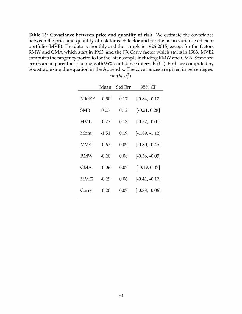
Table 15: Covariance between price and quantity of risk. We estimate the covariancebetween the price and quantity of risk for each factor and for the mean variance efficientportfolio (MVE). The data is monthly and the sample is 1926-2015, except for the factorsRMW and CMA which start in 1963, and the FX Carry factor which starts in 1983. MVE2computes the tangency portfolio for the later sample including RMW and CMA. Standarderrors are in parentheses along with 95% confidence intervals (CI). Both are computed bybootstrap using the equation in the Appendix. The covariances are given in percentages.

cov(bt, σ2t )

Mean Std Err 95% CI

MktRF -0.50 0.17 [-0.84, -0.17]

SMB 0.03 0.12 [-0.21, 0.28]

HML -0.27 0.13 [-0.52, -0.01]

Mom -1.51 0.19 [-1.89, -1.12]

MVE -0.62 0.09 [-0.80, -0.45]

RMW -0.20 0.08 [-0.36, -0.05]

CMA -0.06 0.07 [-0.19, 0.07]

MVE2 -0.29 0.06 [-0.41, -0.17]

Carry -0.20 0.07 [-0.33, -0.06]

64

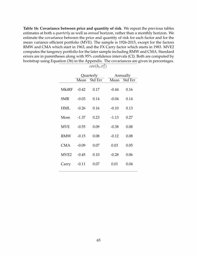
Table 16: Covariance between price and quantity of risk. We repeat the previous tablesestimates at both a quarterly as well as annual horizon, rather than a monthly horizon. Weestimate the covariance between the price and quantity of risk for each factor and for themean variance efficient portfolio (MVE). The sample is 1926-2015, except for the factorsRMW and CMA which start in 1963, and the FX Carry factor which starts in 1983. MVE2computes the tangency portfolio for the later sample including RMW and CMA. Standarderrors are in parentheses along with 95% confidence intervals (CI). Both are computed bybootstrap using Equation (36) in the Appendix. The covariances are given in percentages.

cov(bt, σ2t )

Quarterly AnnuallyMean Std Err Mean Std Err

MktRF -0.42 0.17 -0.44 0.16

SMB -0.03 0.14 -0.04 0.14

HML -0.26 0.16 -0.10 0.13

Mom -1.37 0.23 -1.13 0.27

MVE -0.55 0.09 -0.38 0.08

RMW -0.15 0.08 -0.12 0.08

CMA -0.09 0.07 0.03 0.05

MVE2 -0.45 0.10 -0.28 0.06

Carry -0.11 0.07 0.01 0.04

65