Vol.7, No.3, pp.183–191, September 2013 DOI … · 1939c), American Concrete Institute (ACI) 209 (Tech. Rep. ACI 209R-92, 1992) and CEB-FIP (CEB-FIP Model Code, 2010). A a typical

Effect of a Time Dependent Concrete Modulus of Elasticityon Prestress Losses in Bridge Girders

Brahama P. Singh1), Nur Yazdani2),*, and Guillermo Ramirez3)

(Received November 13, 2012, Accepted March 21, 2013)

Abstract: Prestress losses assumed for bridge girder design and deflection analyses are dependent on the concrete modulus of

elasticity (MOE). Most design specifications, such as the American Association of State Highways and Transportation Officials

(AASHTO) bridge specifications, contain a constant value for the MOE based on the unit weight of concrete and the concrete

compressive strength at 28 days. It has been shown in the past that that the concrete MOE varies with the age of concrete. The

purpose of this study was to evaluate the effect of a time-dependent and variable MOE on the prestress losses assumed for bridge

girder design. For this purpose, three different variable MOE models from the literature were investigated: Dischinger (Der

Bauingenieur 47/48(20):563–572, 1939a; Der Bauingenieur 5/6(20):53–63, 1939b; Der Bauingenieur, 21/22(20):286–437,

1939c), American Concrete Institute (ACI) 209 (Tech. Rep. ACI 209R-92, 1992) and CEB-FIP (CEB-FIP Model Code, 2010). A

typical bridge layout for the Dallas, Texas, USA, area was assumed herein. A prestressed concrete beam design and analysis

program from the Texas Department of Transportation (TxDOT) was utilized to determine the prestress losses. The values of the

time dependent MOE and also specific prestress losses from each model were compared. The MOE predictions based on the ACI

and the CEB-FIP models were close to each other; in long-term, they approach the constant AASHTO value. Dischinger’s model

provides for higher MOE values. The elastic shortening and the long term losses from the variable MOE models are lower than that

using a constant MOE up to deck casting time. In long term, the variable MOE-based losses approach that from the constant MOE

predictions. The Dischinger model would result in more conservative girder design while the ACI and the CEB-FIP models would

result in designs more consistent with the AASHTO approach.

Keywords: concrete modulus of elasticity, prestress losses, bridge girders, I-girders.

1. Introduction

The purpose of this study was to examine several existingtime dependent moduli of elasticity (MOE) of concrete andevaluate their effect on various prestress losses in typicalbridge girders. Towards this end, a method proposed byDischinger (1939a, b, c) for a variable MOE was consideredherein, along with a couple of other methods from the lit-erature. The MOE from Dischinger’s method varies with theconcrete creep function. The current American Associationof State Highways and Transportation Officials (AASHTO)specifications consider the concrete MOE to remain constantthrough the life of a structure (AASHTO 2010). AASHTO’s

calculation of the concrete MOE is based on the unitweight and the 28 day compressive strength of concrete.The two additional methods considered herein were theAmerican Concrete Institute (ACI) 209 Model Code (1992)and CEB-FIP 1990 Model Code (2010). A realistic con-crete MOE that varies with concrete age is likely to resultin more precise estimation of various prestress losses inconcrete girders, resulting in more realistic girder design,prestress estimation, camber calculations and bridge deckdesign/construction.Equations for variable MOE of concrete considering types

of mineral admixtures and coarse aggregates were developedpreviously (Nemati 2006). Valuable data and general trendsin concrete strengths, creep coefficient and MOE for typicalFlorida concrete were generated through another study (Tiaet al. 2005). Yazdani et al. (2005) developed concrete MOEmodels based on aggregate classes in Florida and a variableconcrete strength. There have been no other studies in thepast in which the effects of a variable and time dependentconcrete MOE on prestress losses were investigated.

1.1 AASHTO ApproachThe AASHTO regulates highway bridge design in the

United States. Currently, all bridge design in the state ofTexas is performed in accordance with the AASHTO LRFD

1)Bridge Division, Dallas District, Texas Department of

Transportation, Mesquite, TX 75150, USA.2)Department of Civil Engineering, University of Texas

at Arlington, Arlington, TX 76019, USA.

*Corresponding Author; E-mail: [email protected])Buildings and Structures, Exponent, Houston,

TX 77042, USA.

Copyright � The Author(s) 2013. This article is published

with open access at Springerlink.com

International Journal of Concrete Structures and MaterialsVol.7, No.3, pp.183–191, September 2013DOI 10.1007/s40069-013-0037-0ISSN 1976-0485 / eISSN 2234-1315

183

(Load and Resistance Factor Design) 2007 specifications(TxDOT 2012). The constant MOE of concrete as specifiedby AASHTO Equation 5.4.2.4-1 (in U.S. units), reproducedin its SI form in Eq. (1).

Ec ¼ 0:043� w1:5c �

ffiffiffiffi

f 0c

q

ð1Þ

where Ec is the concrete MOE (MPa), wc is the unit weightof concrete (kg/m3), and f0c is the 28 day compressivestrength of concrete (MPa).Equation (1) is valid for concrete with unit weights in the

range of 1,442 kg/m3 (0.90 lbs/ft3) and 2,483 kg/m3 (155 lbs/ft3). The Texas Department of Transportation (TxDOT) con-siders this equation valid for 28 day compressive strengths upto 58.6 MPa (8.5 ksi) (TxDOT 2005). For the purposes of thiswork, the unit weight of concrete was taken as 2,403 kg/m3

(150 lbs/ft3). The MOE for prestressing strands was taken as196.5 GPa (28,500 ksi) per AASHTOLRFDSection 5.4.4.2.AASHTO LRFD Equation 5.9.5.1-1 expresses the prestressloss in girders, as follows:

DfpT ¼ DfpES þ DfpLT ð2Þ

where DfpT is the total loss, DfpES is the loss due to elasticshortening, and DfpLT is the losses due to long-term shrinkageand creep of concrete, and steel relaxationThe loss due toelastic shortening of concrete is given by AASHTOEquation 5.9.5.2.3a-1, as follows:

DfpES ¼ Ep

Eci� fcgp ð3Þ

where Ep is the MOE of prestressing steel, Eci is the MOE ofconcrete at transfer, and fcgp is the sum of concrete stresses atthe center of gravity of prestressing tendons due to theprestressing force at transfer and the self-weight of themember at the sections of maximum moment.The long-term loss is given by AASHTO Equa-

tion 5.9.5.3-1, and is reproduced in Eq. (4). In this equation,the first term corresponds to creep loss, the second term toshrinkage loss and the third to relaxation losses.

DfpLT ¼ 10:0fpiAps

Agchcst þ 12:0chcst þ Dfpr ð4Þ

where H is the average annual ambient relative humidity (%)

ch ¼ 1:7� 0:01Hð Þ AASHTO Eq: 5:9:5:3-2ð Þ ð5Þ

cst ¼5

1þ f0ci

AASHTO Eq: 5:9:5:3-3ð Þ ð6Þ

fpi is the prestressing steel stress prior to transfer, f0ci is thespecified concrete compressive strength at time of prestress-ing, Aps is the area of prestressing steel, Ag is the gross crosssectional area of girder, ch is the correction factor for relativehumidity, cst is the correction factor for specified concretestrength at transfer, and Dfpr is the estimation of relaxationloss, taken as 16.6 MPa (2.4 ksi) for low relaxation strands.

1.2 Dischinger MethodFranz Dischinger (1887–1953) was a well-known German

civil and structural engineer who was responsible for thedevelopment of the modern cable-stayed bridge. He isknown for his work in prestressed concrete and, in 1939,published a theory called ‘‘Elastic and Plastic Distortions ofReinforced Concrete Structural Members and in Particular ofArched Bridges’’ (1939a, b, c). Dischinger showed that theMOE is a function of time since the creep of concrete is alsoa function of time. Dischinger’s evaluation of the change inconcrete MOE with time was based on a creep coefficientdetermined from laboratory tests. He proposed the followingequation for concrete MOE:

Eot ¼ Eo 1þ wtð Þ ð7Þ

where Eot is the modified MOE at time t, Eo is the initialMOE, and wt is the creep coefficientAASHTO specifies a concrete creep coefficient (AASHTO

Equation 5.4.2.3.2-1), as follows:

wðt; tiÞ ¼ 1:9kskhckf ktdt�0:118i ð8Þ

where

ks ¼ 1:45� 0:13V

S

� �

� 1:0 AASHTO 5:4:2:3:2-2

ð9Þ

khc ¼ 1:56� 0:008H AASHTO 5:4:2:3:2-3 ð10Þ

kf ¼5

1þ f0ci

AASHTO 5:4:2:3:2-4 ð11Þ

ktd ¼t

61� 4f0ci þ t

AASHTO 5:4:2:3:2-4 ð12Þ

ks is the factor for effect of volume to surface ratio, kf is thefactor for the effect of concrete strength, khc is the humidityfactor for creep, ktd is the time dependent factor, V/S is thevolume to surface ratio, t is the time (days), and ti is the ageof concrete at time of load application (days).In this study, the creep coefficient from Eq. (8) was calcu-

lated and used as the basis for the Dischinger Model (Eq. (7)).

1.3 ACI 209 MethodThe ACI 209 Model Code (1992) specifies a time

dependent concrete MOE based on a time dependent 28 daycompressive strength. The time variable compressivestrength (ACI Eq. 2.1) is as follows:

f0

c tð Þ ¼ t

aþ btf0

c

� �

28ð13Þ

where f0c(t) is the compressive strength at time t; t is the time indays; (f0c)28 is the 28 day compressive strength; and a andb areconstants depending on curing and cement type, respectively.The values for a and b are reproduced in Table 1. For this

study, Type I cement and moist cured concrete wereassumed. When girders are manufactured, the concrete is

184 | International Journal of Concrete Structures and Materials (Vol.7, No.3, September 2013)

normally steam cured to allow for quick turnaround. Bothsteam and moist curing were checked herein to note thedifference in the values for the MOE. The difference in MOEwas not significant for either curing type. ACI Equa-tion 20.25 for the variable MOE is given in Eq. (14).

Ec tð Þ ¼ 0:043ffiffiffiffiffiffiffiffiffiffiffiffiffiffi

w3f 0c ðtÞ

q

ð14Þ

where Ec(t) is the MOE of concrete at age t days (MPa), w isthe unit weight of concrete (kg/m3), and f0c(t) is the com-pressive strength at time t in days (MPa, Eq. (13)).

1.4 The CEB-FIP MethodThe CEB-FIP Model Code (2010) was initially published

in 1978 and since then has impacted national codes in manycountries. ACI and other well-known codes have referencedthe CEB-FIP Code in their publications. The CEB-FIP givestime dependent concrete MOE is given in CEB-FIP Eq. 2.1-57, and presented in the following:

Eci tð Þ ¼ bEðtÞEci ð15Þ

where Eci(t) is the concrete MOE at an age of t days, Eci isthe concrete MOE at an age of 28 days, and bE(t) is acoefficient depending on the age of concrete (t days); it isgiven by CEB-FIP Eq. 2.1-58 and is as follows:

bE tð Þ ¼ bccðtÞ½ �0:5 ð16Þ

where bcc(t) is a coefficient depending on the age of concrete(t days), given by CEB-FIP Eq. 2.1-54 and as follows:

bcc tð Þ ¼ exp s 1� 28t=t1

!0:58

<

:

9

=

;

2

4

3

5 ð17Þ

where t is the age of concrete (days), t1 is 1 day, s is a coeffi-cient which depends on the type of cement; s = 0.20 for rapidhardening high strength cements, 0.25 for normal and rapidhardening cements and 0.38 for slowly hardening cements. Inthis study, normal hardening cement was assumed. The CEB-FIPCode accounts formaturity of the concrete by allowing thetime in days to be adjusted for temperature. In this study, thistemperature effect on concrete maturity was not considered.The example bridge location for this study (as described later)was assumed to be in a stable environment with the temper-ature range per season to remain fairly constant.

2. PSTRS14 Software

The TxDOT developed and maintains the PrestressedConcrete Beam Design and Analysis Program (PSTRS14)(TxDOT 2007). PSTRS14 designs and analyzes standardTxDOT I, TxGirder, Box, U, Double-T, Slab, and non-standard girders (user defined) with low-relaxation or stress-relieved strands. PSTRS14 includes a standard beam sectionlibrary; however, the user can define unique and non-stan-dard shapes and properties of beams. Furthermore,PSTRS14 assigns default values of material properties.However, the user may also define material properties ofbeams, slabs, shear keys, and even non-standard compositeregions.PSTRS14 only analyzes and designs simply supported

pretensioned concrete beams with draped or straight seven-wire patterns. Straight strands can be debonded; however,draped strands have to be fully bonded. PSTRS14 cansimultaneously solve the required strand pattern (includingnumber of required strands), the release and final requiredconcrete strengths. PSTR14 version 4.2 was used for thestudy herein. This version designs and analyzes prestressedconcrete beams based on AASHTO LRFD Specifications(5th Edition, 2010), AASHTO Standard Specifications forHighway Bridges (17th Edition, 2002), AASHTO StandardSpecifications for Highway Bridges (15th Edition, 1994Interim), American Standard Building Code Requirementsfor Reinforced Concrete (1989) or the American RailwayEngineering Association Specifications (1988).PSTRS14 is a MS-DOS based system in which a text file

is input with material properties, loading and design con-siderations for a prestressed concrete beam. If values are notentered, the program assumes a set of defaults; however, theuser must specify basic information about the beam for thedesign. This basic information includes the following: beamtype (standard name or non-standard), span length (mea-sured center to center of bearing), beam spacing, slabthickness, composite slab width, live load distribution factor,relative humidity, uniform dead load on composite sectiondue to overlay and the uniform dead load on compositesection excluding overlay. PSTRS14 allows the user to selectthe type of output generated. The short summary gives thefollowing information: the number of strands and theireccentricity, draped or bonded strands and how much theyare draped or bonded, design stresses, ultimate momentrequired, camber, dead load deflections due to the slab,

Table 1 Coefficients from ACI 209 model code.

Cement type Curing Duration

I III ts (days)

Strength

a 4.0 2.3 Moist

1.0 0.7 Steam

b 0.85 0.92 Moist

0.95 0.98 Steam

International Journal of Concrete Structures and Materials (Vol.7, No.3, September 2013) | 185

overlay, other loads and the total deflection. For each beamthat is to be designed the long format results includemoment, shear, stress, and prestress loss tables.

3. Sample Bridge Description

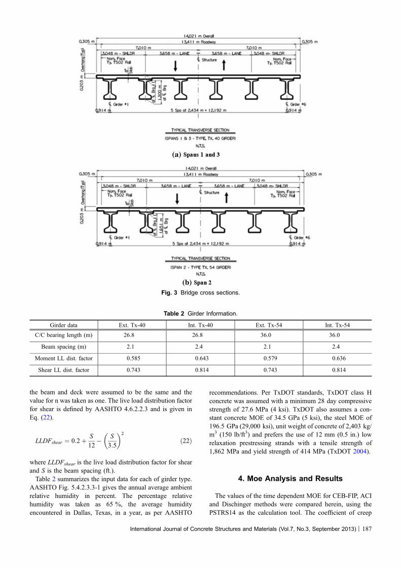
A hypothetical sample bridge was analyzed to evaluate thedifferences between Dischinger’s modified MOE, the ACI209 and the CEB-FIPModels for a variableMOE. The typicalbridgewas assumed to be located in Dallas, Texas, USAwith atotal length of 91.4 m (300 ft.) and three prestressed spans. Asshown in Fig. 1, the bridge consisted of two 27.4 m (90 ft.)spans with Tx-40 girders and one 36.6 m (120 ft.) span withTx-54 girders, standard shapes used by the TxDOT (2010). A13.4 m (44 ft.) wide roadway without a skew was modeled.With a 0.3 m (1 ft.) nominal face of rail assumed, an overallwidth of 13.7 m (46 ft.) was obtained, as shown in Fig. 2. Two3.7 m (12 ft.) travel lanes and a 3 m (10 ft.) shoulder on eachside were assumed. The bridge was modeled with a 200 mm(8 in.) cast in place concrete slab and a 75 mm (3 in.) haunchover the beams. Six girders per span were used at a spacing of2.4 m (8 ft.) with a 0.9 m (3 ft.) overhang. The bridge crosssections are shown in Fig. 3. A type T502 traffic railing wasmodeled for this bridge, a standard crash tested TxDOT rail.This railing is applicable for design speeds greater than80.5 kph (50 miles/h).

3.1 PSTRS14 Software InputThe standard Tx-40 Girder was input into PSTRS14 in

two separate designs: as an exterior and an interior girder,

due to different tributary girder spacing. The girder tributaryspacing was calculated by Eq. 18 (TxDOT 2012).

St ¼S

2þ OH ð18Þ

where St is the effective beam spacing, S is the interiorcenterline to centerline beam spacing, and OH is the width ofoverhang of exterior beam.Using the spacing, the live load distribution factors for

moment and shear were calculated and input into PSTRS14.Equation (19) comes from AASHTO 4.6.2.2.2 and calcu-lates the live load distribution factor for moment.

LLDFm ¼ 0:075þ S

9:5

0:6

� S

L

0:2

� Kg

12Lt3s

� �0:1

ð19Þ

where LLDFm is the live load distribution factor for moment,S is the beam spacing, L is the length of beam (centerlinebearing to centerline bearing), ts is the slab thickness (in.),and Kg is defined in Eq. (20).

Kg ¼ nðI þ Ae2gÞ ð20Þ

where I is the moment of inertia of the beam (in4), A is thearea of the beam (in2), eg is the distance between center ofgravity of beam and deck (in.), and n is defined in Eq. (21).

n ¼ Ebeam

Edeckð21Þ

where Ebeam is the MOE of the beam concrete and Edeck isthe MOE of the deck concreteFor this bridge, the modulus of

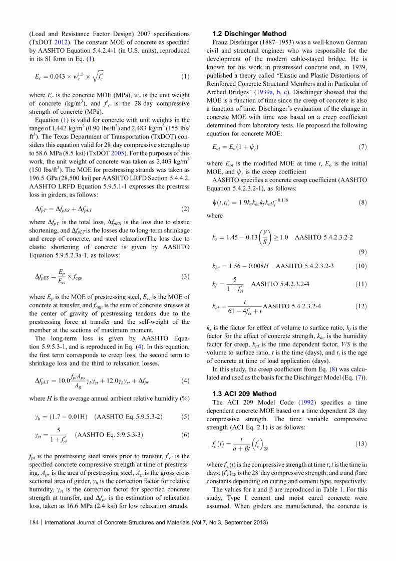
Fig. 1 Profile view of model bridge.

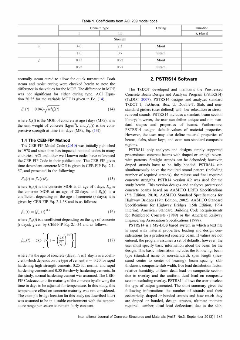
Fig. 2 Plan view of model bridge.


the beam and deck were assumed to be the same and thevalue for n was taken as one. The live load distribution factorfor shear is defined by AASHTO 4.6.2.2.3 and is given inEq. (22).

LLDFshear ¼ 0:2þ S

12� S

3:5

� �2

ð22Þ

where LLDFshear is the live load distribution factor for shearand S is the beam spacing (ft.).Table 2 summarizes the input data for each of girder type.

AASHTO Fig. 5.4.2.3.3-1 gives the annual average ambientrelative humidity in percent. The percentage relativehumidity was taken as 65 %, the average humidityencountered in Dallas, Texas, in a year, as per AASHTO

recommendations. Per TxDOT standards, TxDOT class Hconcrete was assumed with a minimum 28 day compressivestrength of 27.6 MPa (4 ksi). TxDOT also assumes a con-stant concrete MOE of 34.5 GPa (5 ksi), the steel MOE of196.5 GPa (29,000 ksi), unit weight of concrete of 2,403 kg/m3 (150 lb/ft3) and prefers the use of 12 mm (0.5 in.) lowrelaxation prestressing strands with a tensile strength of1,862 MPa and yield strength of 414 MPa (TxDOT 2004).

4. Moe Analysis and Results

The values of the time dependent MOE for CEB-FIP, ACIand Dischinger methods were compared herein, using thePSTRS14 as the calculation tool. The coefficient of creep

Fig. 3 Bridge cross sections.

Table 2 Girder Information.

Girder data Ext. Tx-40 Int. Tx-40 Ext. Tx-54 Int. Tx-54

C/C bearing length (m) 26.8 26.8 36.0 36.0

Beam spacing (m) 2.1 2.4 2.1 2.4

Moment LL dist. factor 0.585 0.643 0.579 0.636

Shear LL dist. factor 0.743 0.814 0.743 0.814


used in Dischinger’s MOE model was assumed to be thesame for the Tx-40 and Tx-54 girders since the volume tosurface area ratio variation in Eq. (9) can be a maximum of152 mm (6 in.) per AASHTO 5.4.2.3.2. This upper limitcontrolled for both girder types. The constants a and b (Table 1)were assumed as 4 and 0.85, respectively. The concrete strengthfactor kf (Eq. (11)) was found to be 0.8973.The girders were analyzed for time intervals representing

various stages of construction (Table 3). The time wasmeasured from the day the girder was cast (day 1). PerTxDOT standard specifications, the girder must be cured fora minimum of 10 days. Once a girder is cured and passes theinspection processes, it is typically shipped directly to thejobsite or stored at the yard. It was assumed herein that aftercuring, it is shipped to the jobsite within 4 days. It is difficultto evaluate when construction loads/permanent dead loads(of the deck) are placed on the girder since each project andcontractor schedule are different. For this analysis, a timeframe of 3 months was assumed until the deck was cast andanother 1 month until the railing was placed. This bridgewas assumed to be open to traffic 4 months after the railingwas cast. Table 4 gives various calculated parameters forMOE calculation for these time intervals. In order to furtheranalyze long-term MOEs, longer time frames of 1, 2, 5 yearsand up to 50 years (assumed life of bridge) were alsoinvestigated. The corresponding calculated MOE parametersare presented in Table 5.

Plots of the calculated MOE values for various construc-tion time sequences and longer time frames are presented inFigs. 4 and 5, respectively. It can be seen from Fig. 4 thatthe MOE from the ACI 209 and the CEB-FIP Models are inclose agreement. These values become almost constant afterthe time interval assumed for the deck casting (104 days).Furthermore, the ACI and the CEB-FIP values reach amaximum MOE of around 37 GPa (5,387 ksi), which isclose to the constant value used by TxDOT (34.4 GPa or5,000 ksi). Dischinger’s proposed method for the MOEshows significantly higher values, as compared to ACI andCEB-FIP models, and continues to increase for the durationof the construction period. This significant difference may beattributed to the nature of the Dischinger’s model (Eq. (7)).This equation depends linearly on the creep coefficient andincreases as the creep coefficient increases. Because thecreep coefficient is linearly dependent upon time (Eq. (8)),the Dischinger equation yields MOE values that are timedependent. As seen in Eqs. (14) and (15), the MOE valuesfrom the ACI 209 and the CEB-FIP models are functions ofthe square root of the time-dependent concrete compressivestrength. So, unlike the CEB-FIP and the ACI 209 Methodpredictions, the Dischinger Method continues to show asignificant increase in MOE after the deck casting. Figure 5shows that the MOE from the ACI and the CEB-FIP modelsremain almost constant throughout the service life. However,the values predicted by Dischinger Model increases slightly,

Table 3 Construction time intervals used for MOE analysis.

tfinal (days) Description

2 Initial stress transfer

10 Girder curing

14 Girder placement at jobsite

104 Casting of deck on girders

134 Casting of railing

254 Bridge opening to traffic

365 At 1 year

730 At 2 years

Table 4 MOE calculation parameters during construction time intervals.

tfinal (days) kc [Eq. (11)] Creep coefficient, w [Eq. (9)] ACI f0c(t), MPa [Eq. (12)]

2 0.149 0.04 1,404

10 0.169 0.15 3,200

14 0.178 0.18 3,522

104 0.327 0.66 4,502

134 0.360 0.77 4,546

254 0.451 1.08 4,620

365 0.502 1.27 4,646

730 0.586 1.60 4,676


yet remain fairly close to approximately 110 GPa(16,000 ksi).

4.1 Effects of Variable MOE on PrestressLosses During ConstructionThe PSTRS14 summary output contained predicted values

of different types of prestress losses, percentage of losses atrelease and a final value. In this study, the effect of variableMOE was investigated on elastic shortening and creep lossesduring the construction time sequences. Since the relativehumidity was taken to be constant, the effect on shrinkagelosses was not evaluated.The dead load due to overlay and railing was input into

PSTRS14. Other loads included the dead load of the slab andthe live load. The live load was automatically calculated byPSTRS14basedon theAASHTOLRFDspecifications. For thisstudy, a 50 mm (2 in.) overlay thickness was assumed. TxDOTcalculates this uniform dead load due to overlay as 37 kg/m(0.025 kip/ft). To determine the load per girder, this dead loadwas multiplied by the beam spacing, as shown in Eq. 23.

DLoverlay ¼ DL� S ð23Þ

where DLoverlay is the uniform dead load due to overlay pergirder, DL is the uniform dead load due to overlay, and S isthe beam spacing (varies for interior and exterior girders)

For exterior girders, the tributary spacing was used tocalculate the dead load. In the case of this model bridge, nosidewalks or temporary railings were assumed. From theTxDOT bridge railing standards (TxDOT 2012), the uniformdead load for the railing was found as 466 kg/m (0.313 kip/ft.). To find the dead load per girder, the total uniform deadload from both rails was divided by the number of girders inthe span. In the model bridge, the number of beams in allspans was the same, resulting in identical dead loads.Table 6 gives the values for the superimposed dead loads. Adefault value for the live load impact factor of 1.33 wasassumed by the software for the HL-93 live load fromAASHTO.The elastic shortening loss results from PSTRS14 with the

variable MOE inputs for the Tx-40 exterior and interiorgirders are shown in Figs. 6 and 7. As seen in Eq. 7, theDischinger MOE model is only dependent on the initialconcrete compressive strength (linearly), while the ACI 209

Table 5 MOE calculation parameters for 5–50 years.

tfinal (years) kc (Eq. 11) Creep coefficient, w (Eq. 8) ACI f0c(t), MPa (Eq. 13)

5 0.659 1.94 4,698

10 0.689 2.09 4,700

15 0.700 2.16 4,702

20 0.705 2.19 4,703

25 0.709 2.22 4,703

30 0.711 2.23 4,704

35 0.713 2.25 4,704

40 0.714 2.26 4,704

45 0.715 2.26 4,704

50 0.716 2.27 4,705

Fig. 4 Variation of MOE for construction time intervals. Fig. 5 Variation of MOE from 5 to 50 years.

Table 6 Dead load for girders (kg/m).

Load Exterior girder Interior girder

Due to overlay 260 298

Due to railing 155 155


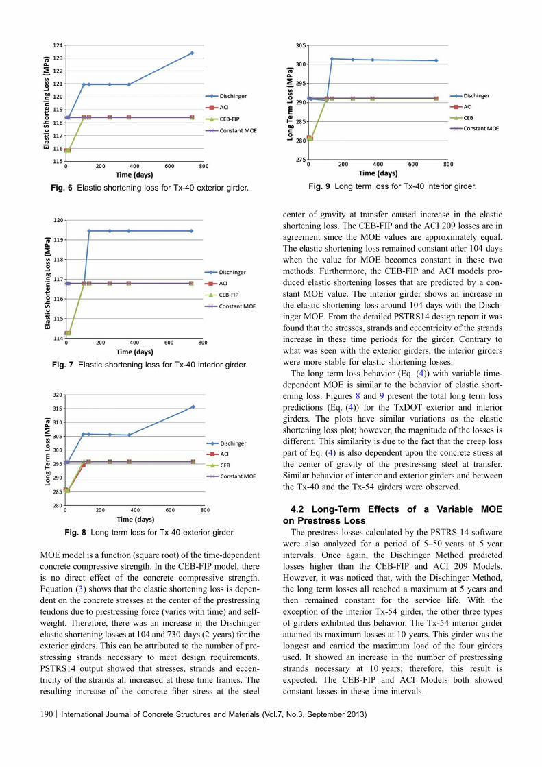
MOE model is a function (square root) of the time-dependentconcrete compressive strength. In the CEB-FIP model, thereis no direct effect of the concrete compressive strength.Equation (3) shows that the elastic shortening loss is depen-dent on the concrete stresses at the center of the prestressingtendons due to prestressing force (varies with time) and self-weight. Therefore, there was an increase in the Dischingerelastic shortening losses at 104 and 730 days (2 years) for theexterior girders. This can be attributed to the number of pre-stressing strands necessary to meet design requirements.PSTRS14 output showed that stresses, strands and eccen-tricity of the strands all increased at these time frames. Theresulting increase of the concrete fiber stress at the steel

center of gravity at transfer caused increase in the elasticshortening loss. The CEB-FIP and the ACI 209 losses are inagreement since the MOE values are approximately equal.The elastic shortening loss remained constant after 104 dayswhen the value for MOE becomes constant in these twomethods. Furthermore, the CEB-FIP and ACI models pro-duced elastic shortening losses that are predicted by a con-stant MOE value. The interior girder shows an increase inthe elastic shortening loss around 104 days with the Disch-inger MOE. From the detailed PSTRS14 design report it wasfound that the stresses, strands and eccentricity of the strandsincrease in these time periods for the girder. Contrary towhat was seen with the exterior girders, the interior girderswere more stable for elastic shortening losses.The long term loss behavior (Eq. (4)) with variable time-

dependent MOE is similar to the behavior of elastic short-ening loss. Figures 8 and 9 present the total long term losspredictions (Eq. (4)) for the TxDOT exterior and interiorgirders. The plots have similar variations as the elasticshortening loss plot; however, the magnitude of the losses isdifferent. This similarity is due to the fact that the creep losspart of Eq. (4) is also dependent upon the concrete stress atthe center of gravity of the prestressing steel at transfer.Similar behavior of interior and exterior girders and betweenthe Tx-40 and the Tx-54 girders were observed.

4.2 Long-Term Effects of a Variable MOEon Prestress LossThe prestress losses calculated by the PSTRS 14 software

were also analyzed for a period of 5–50 years at 5 yearintervals. Once again, the Dischinger Method predictedlosses higher than the CEB-FIP and ACI 209 Models.However, it was noticed that, with the Dischinger Method,the long term losses all reached a maximum at 5 years andthen remained constant for the service life. With theexception of the interior Tx-54 girder, the other three typesof girders exhibited this behavior. The Tx-54 interior girderattained its maximum losses at 10 years. This girder was thelongest and carried the maximum load of the four girdersused. It showed an increase in the number of prestressingstrands necessary at 10 years; therefore, this result isexpected. The CEB-FIP and ACI Models both showedconstant losses in these time intervals.

Fig. 6 Elastic shortening loss for Tx-40 exterior girder.

Fig. 7 Elastic shortening loss for Tx-40 interior girder.

Fig. 8 Long term loss for Tx-40 exterior girder.

Fig. 9 Long term loss for Tx-40 interior girder.


5. Conclusions

The following conclusions may be made based on thefindings from this study:

1. The time dependent concrete MOE predicted by the ACI209 and the CEB-FIP models are in close agreement forshort term as well as long term situations. These valuesbecome approximately constant after the deck casting at104 days. The predictions from the two modelsapproach the constant MOE value recommended byAASHTO and TxDOT specifications (34.4 GPa).

2. At initial conditions (less than 14 days after casting), thecode specified constant MOE is greater than the MOEspredicted by ACI and CEB-FIP. At 2 days, the differ-ence is almost 55 %.

3. The MOEs from the ACI and the CEB-FIP modelsresult in elastic shortening losses that were less than thatresulting from the constant MOE up to 104 days aftercasting. However, the differences are small (around4 %). After this time, the elastic shortening lossesapproached the constant value. The Dischinger predic-tion for this loss was slightly higher. Similar trends werenoted for exterior and interior girders.

4. The variations in the long term losses were similar tothat for the elastic shortening losses. This similarity isdue to the fact that both loss types are dependent on theconcrete stress at the center of gravity of the prestressingsteel at transfer.

5. The use of Dischinger’s method would produce a moreconservative beam design in general, as opposed to thatfor the constant or the ACI/CEB-FIP models.

6. Dischinger’s method provides a simple approach for thecalculation of a variable MOE. However, the ACI andthe CEB-FIP methods produce MOE and prestress lossvalues that are in close agreement with each other. Theyare also in line with the constant MOE and the resultinglosses for concrete bridge I-girders.

Open Access

This article is distributed under the terms of the CreativeCommons Attribution License which permits any use,distribution, and reproduction in any medium, provided theoriginal author(s) and the source are credited.

References

American Association of State Highway and Transportation

Officials (AASHTO). (2010). AASHTO LRFD Bridge

Design Specifications. 5th Edition, Washington DC, USA.

American Concrete Institute (ACI). (1992). Prediction of creep,

shrinkage, and temperature effects in concrete structures.

Technical Publication. ACI 209R-92.

CEB-FIP. (2010). CEB-FIP Model Code 2010. Comite Euro-

International du Beton.

Dischinger, F. (1939a). Elastiche und Plastische Verformungen

Der Eisenbetontragwerke Und Insbesondere Der Bogen-

brucken. Der Bauingenieur, 47/48 (20), 563–572.

Dischinger, F. (1939b). Elastiche und Plastische Verformungen



Dischinger, F. (1939c). Elastiche und Plastische Verformungen



Nemati, K. M. (2006). Modulus of elasticity of high-strength

concrete. Karachi: CBM-CI International Workshop.

Texas Department of Transportation (TxDOT). (2004). Texas

Department of Transportation standard specifications.

Austin: Texas Department of Transportation.

Texas Department of Transportation (TxDOT). (2005). LRFD

bridge design manual. Austin: Texas Department of

Transportation.

Texas Department of Transportation (TxDOT). (2007). Pre-

stressed concrete beam design/analysis program user

guide. Austin: Texas Department of Transportation.

Texas Department of Transportation (TxDOT). (2010). Bridge

design standards. Austin: TexasDepartment of Transportation.

Texas Department of Transportation (TxDOT). (2012). Bridge

railingmanual. Austin: TexasDepartment of Transportation.

Tia,M., Liu, Y., & Brown, D. (2005).Modulus of elasticity, creep

and shrinkage of concrete. Final report, Florida Department

of Transportation, Contract No. BC-354.

Yazdani, N., McKinnie, B., & Haroon, S. (2005). Aggregate

based modulus of elasticity for Florida concrete. Journal of

Transportation Research Record (TRR), 1914, 15–23.


Documents

Vol.7, No.3, pp.183–191, September 2013 DOI … · 1939c), American Concrete Institute (ACI) 209 (Tech. Rep. ACI 209R-92, 1992) and CEB-FIP (CEB-FIP Model Code, 2010). A a typical