Embed Size (px)
Citation preview

World Scientific
World Scientific Series
in FINANCE vol. 55
Roggi
Altman
vol.
This edited volume presents the most recent achievements
in risk measurement and management, as well as regulation
of the financial industry, with contributions from prominent
scholars and practitioners such as Robert Engle, 2003 Nobel
Laureate in Economics, Viral Acharya, Torben Andersen,
Zvi Bodie, Menachem Brenner, Aswath Damodaran, Marti
Subramanyam, William Ziemba and others. The book provides
a comprehensive overview of recent emerging standards
in risk management from an interdisciplinary perspective.
Individual chapters expound on the theme of standards
setting in this era of financial crises where new and unseen
global risks have emerged. They are organized in a such a
way that allows the reader a broad perspective of the new
emerging standards in macro, systemic and sovereign risk
before zooming into the micro perspective of how risk is
conceived and treated within a corporation. A section is
dedicated to credit risk and to the increased importance of
liquidity both in financial systems and at the firm’s level.
World Scientificwww.worldscientific.com8565 hc
ISBN 978-981-4417-49-5
Editors
Oliviero RoggiEdward Altman
With contributions from
Robert EngleNobel Laureate in Economic Sciences 2003
Viral Acharya Torben AndersenZvi Bodie Menachem BrennerAswath Damodaran Marti SubrahmanyamWilliam Ziemba
Managing and Measuring Risk
Managing and Measuring Risk
Emerging Global Standards andRegulation After the Financial Crisis
Emerging Global Standards andRegulation After the Financial Crisis
Manag
ing and
Measuring
RiskEm
ergin
g G
lobal Sta
ndard
s a
nd R
egula
tion A
fter the Fin
ancia
l Cris
is

Managing and Measuring RiskEmerging Global Standards and
Regulation After the Financial Crisis

November 19, 2012 9:30 9in x 6in Measuring and Managing of Risk b1485-fm 2nd Reading
ii

N E W J E R S E Y • L O N D O N • S I N G A P O R E • B E I J I N G • S H A N G H A I • H O N G K O N G • TA I P E I • C H E N N A I
World Scientific
World Scientific Series
in FINANCE vol.
Editors
Oliviero RoggiUniversity of Florence, Italy & New York University, USA
Edward AltmanNew York University, USA
5
Managing and Measuring RiskEmerging Global Standards and
Regulation After the Financial Crisis

Published by
World Scientific Publishing Co. Pte. Ltd.
5 Toh Tuck Link, Singapore 596224
USA office: 27 Warren Street, Suite 401-402, Hackensack, NJ 07601
UK office: 57 Shelton Street, Covent Garden, London WC2H 9HE
British Library Cataloguing-in-Publication Data
A catalogue record for this book is available from the British Library.
World Scientific Series in Finance — Vol. 5
MANAGING AND MEASURING RISK
Emerging Global Standards and Regulations After the Financial Crisis
Copyright © 2012 by World Scientific Publishing Co. Pte. Ltd.
All rights reserved. This book, or parts thereof, may not be reproduced in any form or by any means,
electronic or mechanical, including photocopying, recording or any information storage and retrieval
system now known or to be invented, without written permission from the Publisher.
For photocopying of material in this volume, please pay a copying fee through the Copyright
Clearance Center, Inc., 222 Rosewood Drive, Danvers, MA 01923, USA. In this case permission to
photocopy is not required from the publisher.
ISBN 978-981-4417-49-5
In-house Editor: Sandhya Venkatesh
Typeset by Stallion Press
Email: [email protected]
Printed in Singapore.
Sandhya - Managing and Measuring Risk2.pmd 11/14/2012, 1:43 PM2

November 19, 2012 9:30 9in x 6in Measuring and Managing of Risk b1485-fm 2nd Reading

November 19, 2012 9:30 9in x 6in Measuring and Managing of Risk b1485-fm 2nd Reading
CONTENTS
Foreword v
About the Editors xiii
Part A. The Evolution of Risk Management 1
Chapter 1. An Evolutionary Perspective on the Concept of Risk,Uncertainty and Risk Management 3Oliviero Roggi and Omar Ottanelli
Part B. Sovereign and Systemic Risk 39
Chapter 2. Toward A Bottom-Up Approach to AssessingSovereign Default Risk: An Update 41Edward I. Altman and Herbert Rijken
Chapter 3. Measuring Systemic Risk 65Viral V. Acharya, Christian Brownlees, Robert Engle,Farhang Farazmand and Matthew Richardson
Chapter 4. Taxing Systemic Risk 99Viral V. Acharya, Lasse Pedersen, Thomas Philipponand Matthew Richardson
Part C. Liquidity 123
Chapter 5. Liquidity and Efficiency in Three Related ForeignExchange Options Markets 125Menachem Brenner and Ben Z. Schreiber
xi

November 19, 2012 9:30 9in x 6in Measuring and Managing of Risk b1485-fm 2nd Reading
xii Contents
Chapter 6. Illiquidity or Credit Deterioration: A Studyof Liquidity in the US Corporate Bond MarketDuring Financial Crises 159Nils Friewald, Rainer Jankowitschand Marti G. Subrahmanyam
Part D. Risk Management Principlesand Strategies 201
Chapter 7. Integrated Wealth and Risk Management:First Principles 203Zvi Bodie
Chapter 8. Analyzing the Impact of Effective Risk Management:Innovation and Capital Structure Effects 215Torben Juul Andersen
Part E. Credit Risk 249
Chapter 9. Modeling Credit Risk for SMEs: Evidencefrom the US Market 251Edward I. Altman and Gabriele Sabato
Chapter 10. SME Rating: Risk Globally, Measure Locally 281Oliviero Roggi and Alessandro Giannozzi
Chapter 11. Credit Loss and Systematic LGD 307Jon Frye and Michael Jacobs Jr.
Part F. Equity Risk and Market Crashes 341
Chapter 12. Equity Risk Premiums (ERP): Determinants,Estimation and Implications — The 2012 Edition 343Aswath Damodaran
Chapter 13. Stock Market Crashes in 2007–2009: Were We Ableto Predict Them? 457William T. Ziemba and Sebastien Lleo

November 19, 2012 8:58 9in x 6in Measuring and Managing of Risk b1485-ch09 2nd Reading
PART E
CREDIT RISK
249

November 19, 2012 8:58 9in x 6in Measuring and Managing of Risk b1485-ch05 2nd Reading
124
November 19, 2012 8:58 9in x 6in Measuring and Managing of Risk b1485-ch11 2nd Reading
Chapter 11
CREDIT LOSS AND SYSTEMATIC LGD∗‡
Jon Frye
Federal Reserve Bank of Chicago, USA
Michael Jacobs Jr.
Office of the Comptroller of the Currency, USA
This chapter presents a model of systematic LGD that is simple and effective.It is simple in that it uses only parameters appearing in standard models. It iseffective in that it survives statistical testing against more complicated models.
Credit loss varies from period to period both because the default rate variesand because the loss given default (LGD) rate varies. The default ratehas been tied to a firm’s probability of default (PD) and to factors thatcause default. The LGD rate has proved more difficult to model becausecontinuous LGD is more subtle than binary default and because LGD dataare fewer in number and lower in quality.
∗The authors thank Irina Barakova, Terry Benzschawel, Andy Feltovich, Brian Gordon,Paul Huck, J. Austin Murphy, Ed Pelz, Michael Pykhtin, and May Tang for comments onprevious versions, and to participants at the 2011 Federal Interagency Risk QuantificationForum, the 2011 International Risk Management Conference, and the First InternationalConference on Credit Analysis and Risk Management. Any views expressed are theauthors’ and do not necessarily represent the views of the management of the FederalReserve Bank of Chicago, the Federal Reserve System, the Office of The Comptroller ofthe Currency or the U.S. Department of the Treasury.‡Any views expressed are the authors’ and do not necessarily represent the views of themanagement of the Federal Reserve Bank of Chicago, the Federal Reserve System, the
Office of The Comptroller of the Currency or the U.S Department of Treasury.
307

November 19, 2012 8:58 9in x 6in Measuring and Managing of Risk b1485-ch11 2nd Reading
308 J. Frye and M. Jacobs
Studies show that the two rates vary together systematically.1 System-atic variation works against the lender, who finds that an increase in thenumber of defaults coincides with an increase in the fraction that is lost ina default. Lenders should therefore anticipate systematic LGD within theircredit portfolio loss models, which are required to account for all materialrisks.
This chapter presents a model of systematic LGD that is simple andeffective. It is simple in that it uses only parameters that are already part ofstandard models. It is effective in that it survives statistical testing againstmore complicated models. It may therefore serve for comparison in tests ofother models of credit risk as well as for purposes of advancing models ofcredit spreads that include premiums for systematic LGD risk.
The LGD model is derived in the next section. The section on researchmethods discusses the style of statistical testing to be used and the directfocus on credit loss modeling, both of which are rare in the portfoliocredit loss literature. Three sections prepare the way for statistical testing.These sections develop the model of credit loss for the finite portfolio,discuss the data to be used for calibration and testing, and introducealternative hypotheses. Two sections perform the statistical tests. The firsttests each exposure cell — the intersection of rating grade and seniority —separately. The second brings together sets of cells: all loans, all bonds,or all instruments. Having survived statistical testing, the LGD model isapplied in the section that precedes the conclusion.
The LGD Model
This section derives the LGD model. It begins with the simplest portfolioof credit exposures and assumes that loss and default vary together. Thisassumption by itself produces a general formula for the relationship of LGDto default. The formula depends on the distributions of loss and default. Wenote that different distributions of loss and default produce similar relation-ships, so we specify a distribution based on convenience and ease of appli-cation. The result is thespecific LGDfunction that appears as Equation (3).
The “asymptotically fined grained homogeneous” portfolio of creditexposures has enough same-sized exposures that there is no need tokeep track individual defaults.2 Only the rates of loss, default, and LGD
1Altman and Karlin (2010); Frye (2000).2Gordy (2003).

November 19, 2012 8:58 9in x 6in Measuring and Managing of Risk b1485-ch11 2nd Reading
Credit Loss and Systematic LGD 309
matter. These rates are random variables, and each one has a probabilitydistribution.
Commonly, researchers develop distributions of LGD and default; fromthese and a connection between them, a distribution of credit loss canbe simulated. The loss model might or might not be inferred explicitly,and it would not be tested for statistical significance. This is one way togenerate credit loss models, but it does not guarantee that a model is a goodone that has been properly controlled for Type I Error. This is unfortunate,because credit loss is the variable that can cause the failure of a financialinstitution.
Because loss is the most important random variable, it is the lossdistribution that we wish to calibrate carefully, and it is the loss modelthat we wish to control for error. We symbolize the cumulative distributionfunctions of the rates of loss and default by CDFLoss and CDFDR.
Our first assumption is that greater default rates and greater loss ratesgo together. This assumption puts very little structure on the variables. It ismuch less restrictive than the common assumption that greater default ratesand greater LGD rates go together. The technical assumption is that theasymptotic distributions of default and loss are comonotonic. This impliesthat the loss rate and the default rate take the same quantile, q, withintheir respective distributions:
CDFLoss [Loss ] = CDFDR[DR] = q (1)
The product of the default rate and the LGD rate equals the loss rate.Therefore, for any value of q, the LGD rate equals the ratio of loss todefault, which in turn depend on q and on inverse cumulative distributionfunctions:
LGD =CDF−1
Loss [q]CDF−1
DR[q]=
CDF−1Loss [CDFDR[DR]]
DR(2)
This expresses the asymptotic LGD rate as a function of the asymptoticdefault rate and it holds true whenever the distributions of loss and defaultare comonotonic. This function might take many forms depending on theforms of the distributions. Since LGD is a function of default, one coulduse Equation (2) to infer a distribution of LGD and study it in isolation;however, we keep the focus on the distribution of loss and on the nature ofan LGD function that is consistent with the distribution of loss.
In particular, we begin with a loss model having only two parameters.If a two-parameter loss model were not rich enough to describe credit loss

November 19, 2012 8:58 9in x 6in Measuring and Managing of Risk b1485-ch11 2nd Reading
310 J. Frye and M. Jacobs
data, a more complicated model could readily show this in a straightforwardstatistical test. The same is true of the default model. Therefore, ourprovisional second assumption is that both credit loss and default havetwo-parameter distributions in the asymptotic portfolio.
Testing this assumption constitutes the greater part of this study.Significant loss models with more than two parameters are not found; atwo-parameter loss model appears to be an adequate description of the lossdata used here. Therefore, this section carries forward the assumption oftwo-parameter distributions of loss and default.
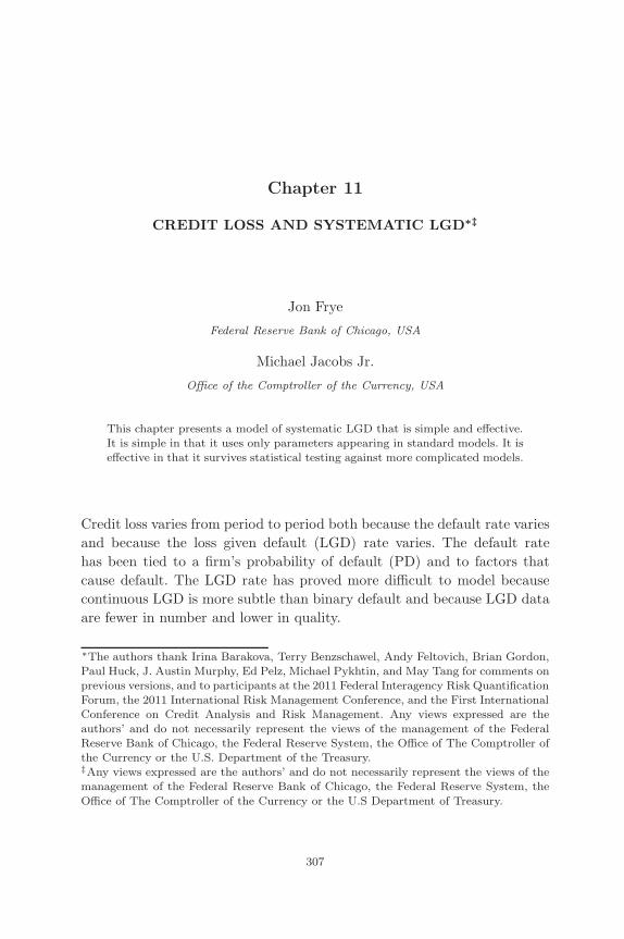
In principle, any two-parameter distributions could be used for theCDFs in Equation (2). In practice, we compare three distributions: Vasicek,Beta, and Lognormal, arranging that each has the same the mean andthat each has the same standard deviation. To obtain values that areeconomically meaningful, we turn to the freely available credit loss datapublished by Altman and Karlin for high-yield bonds, 1989–2007. Themeans and standard deviations appear in the first column of Table 1.The other three columns describe distributions that share these statistics.Figure 1 compares the variants of Equation (2) that result.
As Figure 1 illustrates, the three distributions produce approximatelythe same LGD — default relationship. They differ principally when thedefault rate is low. This is the range in which they would be the mostdifficult to distinguish empirically, because a low default rate generatesfew defaults and substantial random variation in annual average LGD. TheLognormal Distribution produces the relationship with lowest overall slope;however, of the three distributions, the Lognormal has the fattest tail.
Our choice between the distributions is guided by practical consider-ations. Unlike the Beta Distribution, the Vasicek Distribution has explicitformulas for its CDF and its inverse CDF. Unlike Lognormal Distribution,the Vasicek Distribution constrains all rates to be less than 100%. Impor-tantly, estimates of the Vasicek correlation parameter already exist withincurrent credit loss models. This makes the Vasicek distribution, by far, theeasiest for a practitioner to apply. Therefore, our third assumption is thatloss and default obey the Vasicek distribution.
Our fourth assumption is that the value of ρ in CDFLoss equals the valueof ρ in CDFDR. This assumption is testable. Alternative E, introduced later,tests by allowing the values to differ, but it does not find that the valuesare significantly different. Therefore we carry forward the assumption thatthe values of ρ are the same.

November 19, 2012 8:58 9in x 6in Measuring and Managing of Risk b1485-ch11 2nd Reading
Credit Loss and Systematic LGD 311
Table
1:
Calibra
tion
of
Thre
eD
istr
ibuti
ons
toM
ean
and
SD
of
Loss
and
Def
ault
,A
ltm
an-K
arl
inD
ata
,1989–2007.
Vasi
cek
Dis
trib
ution
Bet
aD
istr
ibution
Lognorm
al
Support
0<
x<
10
<x
<1
0<
x<
∞
PD
F[x
]
√1−
ρ√
ρ
φ
» Φ−
1[E
L]−
√1−
ρΦ−
1[x
]√
ρ
–
φ[Φ
−1[x
]]
xa−
1(1
−x)b
−1
Bet
a[a
,b]
Ex
p
» −(L
og[x
]−µ)2
2σ2
–
x√
2π
σ
CD
F[x
]Φ
»√
1−
ρΦ
−1[x
]−
Φ−
1[E
L]
√ρ
–Z
x
0
ya−
1(1
−y)b
−1
Bet
a[a
,b]
dy
1−
Φ
»µ−
Log[x
]
σ
–
CD
F−
1[q
]Φ
»Φ
−1[E
L]+
√ρΦ
−1[q
]√
1−
ρ
–
xsu
chth
at
Exp[µ
−σΦ
−1[1
−q]]
q=
Zx
0
ya−
1(1
−y)b
−1
Bet
a[a
,b]
dy
Calibra
tion
tom
ean
and
standard
dev
iati
on
oflo
ssdata
Mea
n=
2.9
9%
EL
=0.0
299
a=
0.9
024
µ=
−3.8
67
SD
=3.0
5%
ρ=
0.1
553
b=
29.2
8σ
=0.8
445
Calibra
tion
tom
ean
and
standard
dev
iati
on
ofdef
ault
data
Mea
n=
4.5
9%
PD
=0.0
459
a=
1.1
80
µ=
−3.3
69
SD
=4.0
5%
ρ=
0.1
451
b=
24.5
2σ
=0.7
588
φ[·]
sym
bolize
sth
est
andard
norm
alpro
bability
den
sity
funct
ion
Φ[·]
sym
bolize
sth
est
andard
norm
alcu
mula
tive
dis
trib
uti
on
funct
ion
November 19, 2012 8:58 9in x 6in Measuring and Managing of Risk b1485-ch11 2nd Reading
312 J. Frye and M. Jacobs
40%
50%
60%
70%
80%
0% 5% 10% 15% 20%
LGD
Rat
e
Default Rate
Vasicek
Beta
LogNormal
Figure 1: LGD — Default Relationship for Three Distributions.
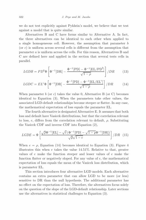
Substituting the expressions for the Vasicek CDF and inverse CDF intoEquation (2) produces the LGD function:
LGD = Φ[Φ−1[DR] − Φ−1[PD] − Φ−1[EL]√
1 − ρ
]/DR
= Φ[Φ−1[DR] − k]/DR (3)
This expresses the asymptotic LGD rate as a function of the asymptoticdefault rate. These rates equal the conditionally expected rates for a singleexposure. Equation (3) underlies the null hypothesis in the tests that follow.
The three parameters PD, EL, and ρ combine to form a single quantitythat we refer to as the LGD Risk Index and symbolize by k. If EL =PD(that is, if ELGD equals 1.0), then k = 0 and LGD=1, irrespective of DR.Except when the LGD Risk Index equals 0, LGD is a strictly monotonicfunction of DR as shown in Appendix 1. For commonly encountered valuesof PD, EL, and ρ, k is between 0 and 2.
To recap, we derive the LGD function by making four assumptions.The first assumption is that a greater rate of credit loss accompanies agreater rate of default. This plausible starting place immediately producesa general expression for LGD, Equation (2). The second assumption isthat the distributions of loss and default each have two parameters.Later sections of this paper attempt, unsuccessfully, to find a statisticallysignificant loss model with more parameters. The third assumption is thatthe distributions are specifically Vasicek. This assumption is a matter ofconvenience; distributions such as Beta and Lognormal produce similarrelationships but they would be more difficult to implement. The fourth

November 19, 2012 8:58 9in x 6in Measuring and Managing of Risk b1485-ch11 2nd Reading
Credit Loss and Systematic LGD 313
assumption is that the value of ρ estimated from default data also appliesto the loss distribution. This assumption is testable, and it survives testingin later sections. The four assumptions jointly imply Equation (3), whichexpresses the LGD rate as a function of the default rate. This LGD functionis consistent with the assumption that credit loss has a two-parameterVasicek distribution.
Research Methods
This section discusses two research methods employed by this paper. First,this paper tests in an unusual way. Rather than showing the statisticalsignificance of Equation (3), it shows the lack of significance of morecomplicated models that allow the LGD-default function to be steeperor flatter than Equation (3). Second, this paper calibrates credit lossmodels to credit loss data. Rather than assume that the parameters ofa credit loss model have been properly established by the study of LGD, itinvestigates credit loss directly.
This study places its preferred model in the role of the null hypothesis.The alternatives explore the space of differing sensitivity by allowing theLGD function to be equal to, steeper than, or flatter than Equation (3).The tests show that none of the alternatives have statistical significancecompared to the null hypothesis. This does not mean that the degreeof systematic LGD risk in Equation (3) can never be rejected, but aworkmanlike attempt has not met with success. Acceptance of a morecomplicated model that had not demonstrated significance would acceptan uncontrolled probability of Type I Error.
A specific hypothesis test has already been alluded to. Equation (3)assumes that the parameter ρ appearing in CDFLoss takes the same valueas the parameter ρ appearing in CDFDR. An alternative allows the twovalues of correlation to differ. This alternative is not found to be statisticallysignificant in tests on several different data sets; the null hypothesis survivesstatistical testing.
We do not try every possible alternative model, nor do we test usingevery possible data set; it is impossible to exhaust all the possibilities.Still, these explorations and statistical tests have content. The functionfor systematic LGD variation is simple, and it survives testing. A riskmanager could use the function as it is. If he prefers, he could test thefunction as we do. A test might show that Equation (3) can be improved.Given, however, that several alternative LGD models do not demonstrate

November 19, 2012 8:58 9in x 6in Measuring and Managing of Risk b1485-ch11 2nd Reading
314 J. Frye and M. Jacobs
significance on a relatively long, extensive, and well-observed data set, anattitude of heightened skepticism is appropriate. In any case, the burdenof proof is always on the model that claims to impart a more detailedunderstanding of the evidence.
The second method used in this paper is to rely on credit loss dataand credit loss models to gain insight into credit risk. By contrast, themodels developed in the last century, such as CreditMetricsTM, treat thedistribution of credit loss as something that can be simulated but notanalyzed directly. This, perhaps, traces back to the fact that twentiethcentury computers ran at less than 1% the speed of current ones, and someshortcuts were needed. But the reason to model LGD and default is toobtain a model of credit loss. The model of credit loss should be the focusof credit loss research, and these days it can be.
We make this difference vivid by a comparison. Suppose a risk managerwants to quantify the credit risk for a specific type of credit exposure.Having only a few years of data, he finds it quite possible that the patternof LGD rates arises by chance. He concludes that the rates of LGD anddefault are independent, and he runs his credit loss model accordingly.This two-stage approach never tests whether independence is valid usingcredit loss data and a credit loss model, and it provides no warrant for thiselision.
Single stage methods are to be preferred because each stage ofstatistical estimation introduces uncertainty. A multi-stage analysis canallow the uncertainty to grow uncontrolled. Single stage methods cancontrol uncertainty. One can model the target variable — credit loss —directly and quantify the control of Type I Error.
The first known study to do this is Frye (2010), which tests whethercredit loss has a two-parameter Vasicek Distribution. One alternative isthat the portfolio LGD rate is independent of the portfolio default rate.3
This produces an asymptotic distribution of loss that has three parameters:ELGD, PD and ρ. The tests show that, far from being statisticallysignificant, the third parameter adds nothing to the explanation of lossdata used.
3The LGD of an individual exposure, since it is already conditioned on the default ofthe exposure, is independent of it. Nonetheless, an LGD can depend on the defaultsof other firms or on their LGDs. This dependence between exposures can producecorrelation between the portfolio LGD rate and the portfolio default rate, therebyaffecting the systematic risk, systematic risk premium, and total required credit spreadon the individual loan.

November 19, 2012 8:58 9in x 6in Measuring and Managing of Risk b1485-ch11 2nd Reading
Credit Loss and Systematic LGD 315
The above illustrates the important difference touched upon earlier.If LGD and default are modeled separately, the implied credit lossdistribution tends to contain all the parameters stemming from eithermodel. By contrast, this paper begins with a parsimonious credit lossmodel and finds the LGD function consistent with it. If a more complicatedcredit loss model were to add something important, it should demonstratestatistical significance in a test.
We hypothesize that credit loss data cannot support extensive the-orizing. This hypothesis is testable, and it might be found wanting.Nevertheless, the current research represents a challenge to portfolio creditloss models running at financial institutions and elsewhere. If those modelshave not demonstrated statistical significance against this approach, theycan be seriously misleading their users.
The current paper extends Frye (2010) in three principal ways. First,it derives and uses distributions that apply to finite-size portfolios. Second,it controlsfor differences of rating and differences of seniority by usingMoody’s exposure-level data. Third, it develops alternative models thatfocus specifically on the steepness of the relationship between LGD anddefault. These are the topics of the next three sections.
The Distribution of Credit Loss in a Finite Portfolio
This section derives the distribution of loss for a portfolio with fewexposures, taking a different approach from the pioneering work by Pykhtinand Dev (2002). Later sections use this distribution to test the LGDfunction against alternatives.
As usual, one must keep separate the concepts related to the populationand the concepts related to the sample. Economic and financial conditionsgive rise to the population variables. These are the conditionally expecteddefault rate, symbolized DR, and the conditionally expected LGD rate,symbolized LGD. LGD is tied to DR by Equation (3) or by one of thealternatives developed later. In a sample of credit loss data, the quantitiesof interest are the number of defaults, D, and the portfolio average LGDrate, LGD .
The derivation begins with DR. Conditioned on DR there is adistribution of D. Conditioned on D, there is a distribution of LGD. Thesedistributions are independent. Their product is the joint distribution of Dand LGD conditioned on DR. The joint distribution of D and LGD istransformed to the joint distribution of D and loss in the usual way.

November 19, 2012 8:58 9in x 6in Measuring and Managing of Risk b1485-ch11 2nd Reading
316 J. Frye and M. Jacobs
The marginal distribution of loss is found by summing over the numberof defaults and removing the conditioning on DR. This produces thedistribution of credit loss when the portfolio is finite.
At the outset we recognize two cases. The first case is that D equals 0.In this case, credit loss equals zero. This case has probability equal to(1–DR)N.
The second case, when D = d > 0, produces a distribution of theportfolio average LGD rate. Average LGD would approach normality forlarge D, according to the Central Limit Theorem. We assume normalityfor all D for two reasons: for convenience, and for the practical benefitthat normality allows average LGD outside the range [0, 1]. This isimportant because the credit loss data includes portfolio-years whereLGD is negative. The variance of the distribution is assumed equalto σ2/d:
fLGD|D=d[LGD] =1
σ/√
dφ
[LGD − LGD
σ/√
d
](4)
The conditional distribution of D and LGD is then the product of theBinomial Distribution of D and the normal distribution of LGD:
fD,LGD|DR[d, LGD] = DRd(1 − DR)N−d
(N
d
)1
σ/√
dφ
[LGD − LGD
σ/√
d
]
(5)
In a portfolio with uniform exposure amounts, the loss rate equals defaultrate times the LGD rate. We pass from the portfolio’s LGD rate to its lossrate with the monotonic transformation:
LGD = N Loss/D; D = D (6)
The Jacobian determinant is N/D. The transformed joint distribution isthen:
fD,Loss|DR [d,Loss ] = DRd(1 − DR)N−d
(N
d
)N
σ√
dφ
[NLoss/d − LGD
σ/√
d
]
(7)

November 19, 2012 8:58 9in x 6in Measuring and Managing of Risk b1485-ch11 2nd Reading
Credit Loss and Systematic LGD 317
Summing over d, combining the two cases, and removing the conditioningon DR produces the distribution of credit loss in the finite portfolio:
fLoss [Loss ] = I[Loss=0][Loss ]∫ 1
0
fDR[DR](1 − DR)N dDR
+ I[Loss>0][Loss ]∫ 1
0
fDR[DR]N∑
d=1
fD,Loss|DR[d,Loss ] dDR
(8)
where fDR[·] is the PDF of the Vasicek density with parameters PD and ρ.This distribution depends on the parameters of the default distribution, PDand ρ. It also depends on any additional parameters of the LGD function.These consist solely of EL in the null hypothesis of Equation (3) but includean additional parameter in the alternatives introduced later. Finally, thedistribution depends on N, the number of exposures. As N increases withoutlimit, Equation (8) becomes the Vasicek distribution with mean equal toEL. For small N, however, the decomposition of EL into PD and ELGDhas an effect on the distribution of loss.
Figure 2 compares the distribution of loss for the asymptotic portfolioto the distribution for a portfolio containing 10 exposures. Each distributionhas EL =5% and ρ = 15%. Those values completely describe the distribu-tion of credit loss in the asymptotic portfolio. For the sake of comparison,EL is assumed decompose to PD= 10% and ELGD=50%. Credit loss inthe finite portfolio has the distribution of Equation (8). The point mass atzero loss has probability 43%; therefore, the area under the curve illustratedin Figure 2 is 57%. Assuming σ = 1% produces distinct humps for one, two,
0
5
10
15
20
25
0% 5% 10% 15% 20%
Den
sity
Credit loss rate
Portfolio with 10 loans:PD = 10%, ELGD = 50%,ρ = 15%, σ = 1%
Asymptotic portfolio:
PD = 10%ELGD = 50%ρ = 15%
Figure 2: Distributions of Loss for Asymptotic and Finite Portfolios.

November 19, 2012 8:58 9in x 6in Measuring and Managing of Risk b1485-ch11 2nd Reading
318 J. Frye and M. Jacobs
and three defaults. The hump for one default is centered at less than 5%loss, while the hump for three defaults is centered at greater than 15% loss.In other words, LGD tends be greater when there are more defaults.
Under the usual statistical assumptions — the parameters are stableover time and the variable DR is independent each year — the log of thelikelihood function of the data is this:
LnLLoss [Loss1,Loss2, . . . ,LossT ] =T∑
t=1
Log[fLoss [Losst]] (9)
Data
The data are twenty-seven years of data drawn from Moody’s CorporateDefault Rate ServiceTM. An exposure “cell” — the intersection of a ratinggrade and a seniority class — controls for both borrower quality andfor exposure quality. A cell is assumed to be a homogenous portfolio ofstatistically identical exposures as called for in the loss models.
Distributions of credit loss can say nothing about cases where theloss amount is unknown. Therefore, we restrict the definition of defaultto cases where Moody’s observes a post-default price. By contrast, studiesof default in isolation can include defaults that produce unknown loss.We refer to this less-restrictive definition as “nominal default” and notethat it produces default rates that are generally greater than the ones wepresent.
We delimit the data set in several ways. To have notched ratingsavailable at the outset, the data sample begins with 1983. To align with theassumption of homogeneity, a firm must be classified as industrial, publicutility, or transportation and headquartered in the US. Ratings are takento be Moody’s “senior” ratings of firms, which usually corresponds to therating of the firm’s long-term senior unsecured debt if such exists. To focuson cells that have numerous defaults, we analyze firms rated Baa3 or lower.We group the ratings C, Ca, Caa, Caa1, Caa2, and Caa3 into a single gradewe designate “C”. This produces five obligor rating grades altogether: Ba3,B1, B2, B3, and C.
To align with the assumption of homogeneity, debt issues must be dollardenominated, intended for the U.S. market, and not guaranteed or otherwisebacked. We define five seniority classes:
• Senior Secured Loans (Senior Secured instruments with Debt Class“Bank Credit Facilities”)

November 19, 2012 8:58 9in x 6in Measuring and Managing of Risk b1485-ch11 2nd Reading
Credit Loss and Systematic LGD 319
• Senior Secured Bonds (Senior Secured instruments with Debt Class“Equipment Trusts”, “First Mortgage Bonds”, or “Regular Bonds/Debentures”)
• Senior Unsecured Bonds (“Regular Bonds/Debentures” or “MediumTerm Notes”)
• Senior Subordinated Bonds (“Regular Bonds/Debentures”)• Subordinated Bonds (“Regular Bonds/Debentures”).
This excludes convertible bonds, preferred stock, and certain otherinstruments.
A firm is defined to be exposed in a cell-year if on January 1st thefirm has one of the five obligor ratings, it is not currently in default, andit has a rated issue in the seniority class. A firm is defined to default ifthere is a record of nominal default and one or more post-default prices areobserved. The LGD of the obligor’s exposures in the cell equals 1.0 minusthe average of such prices expressed as a fraction of par; there is exactlyone LGD for each default. The default rate in the cell-year is the number ofLGD’s divided by the number of firms that are exposed, and the loss rateis the sum of the LGD’s divided by the number of firms that are exposed.There is no correction for firms that are exposed to default for only part ofthe year, perhaps because their debts mature or because their ratings arewithdrawn.
To make ideas concrete, consider the most-populated cell, SeniorSecured Loans made to B2-rated firms. This cell has 1842 cell-years ofexposure. However, public agencies began rating loans only in the latterhalf of the data sample; of the twenty-seven years of the data samplein total, only fourteen years contain loans to B2-rated firms. Of thosefourteen years, only six record a default by a B2-rated firm that had arated loan outstanding. Those six years contain all the information aboutthe LGD-default relationship that is contained within the cell. In all, thecell generates fourteen annual observations on the three variables neededto calibrate the distribution of loss:
• N, the number of exposures• D, the number of defaults, and• Loss, the sum of the LGD’s divided by N, or zero if D = 0.
Alternatives for Testing
This section presents alternative LGD functions that have an additionalparameter and might provide a better fit to the data. Designed to focus on

November 19, 2012 8:58 9in x 6in Measuring and Managing of Risk b1485-ch11 2nd Reading
320 J. Frye and M. Jacobs
a particular question, the alternatives necessarily have a functional formsthat appear more complicated than Equation (3).
In general, a statistical alternative could have any number of functionalforms. For example, one might test Equation (3) against a linear LGDhypothesis:
LGD = u + vDR (10)
Linear Equation (10) can be mentally compared to the curved function forthe Vasicek Distribution that is illustrated in Figure 1. If the straight linewere wholly above the curved line, its expected loss would be too high.Therefore, the straight line and curved line cross. If parameter v takes apositive value, as is likely, the lines cross twice. Therefore, a calibrationof Equation (10) would likely produce a straight line that is shallowerthan Equation (3) at the left and steeper than Equation (3) at the right.If this calibration were statistically significant, the verdict would be thatEquation (3) is too steep in some places and too flat in others.
Such an answer is not without interest, but we address a simplerquestion. If the LGD function of Equation (3) does not adequately representthe data, we want to know whether a better function is steeper or flatter.Therefore our alternatives have a special feature: the additional parameterchanges the LGD-default relationship but has no effect on EL. Whenthe parameter takes a particular value, the alternative becomes identicalto Equation (3), and when the parameter takes a different value, thealternative becomes steeper or flatter than Equation (3). For all values ofthe parameter, the mathematical expectation of loss is equal to the value ofparameter EL. When we test against such an alternative, we are testing for adifference in slope alone. Although the slope of the LGD-default relationshipis not the only aspect of systematic LGD risk that is important, it has first-order importance.
Summarizing, we create alternatives that:
• Contain one more parameter than Equation (3)• Collapse to Equation (3) when the parameter takes a specified value• Are steeper or flatter than Equation (3) otherwise, and,• Produce the same value of EL irrespective of the parameter value.
Alternative A takes the following form, using for convenience the substitu-tion EL =PD ELGD:
LGDA = ELGDaΦ[Φ−1[DR] − Φ−1[PD] − Φ−1[EL/ELGDa]√
1 − ρ
]/DR (11)

November 19, 2012 8:58 9in x 6in Measuring and Managing of Risk b1485-ch11 2nd Reading
Credit Loss and Systematic LGD 321
40%
50%
60%
70%
80%
90%
5% 0% 10% 15% 20%
LGD
Rat
e
Default Rate
a = -2
a = -1
a = 0 (H0)
a = 1
a = 2
Figure 3: Alternative A for Five Values of a.
The additional parameter in Alternative A is symbolized by a. If a takesthe value zero, Alternative A becomes identical to Equation (3). If a
takes the value 1.0, the function collapses to ELGD; in other words, whena = 1 Alternative A becomes a model in which LGD is a constant in theasymptotic portfolio.
Figure 3 illustrates Alternative A for five values of a. If parameter a
takes a negative value, Alternative A is steeper than Equation (3).If parameter a takes a value greater than 1.0, Alternative A is negativelysloped. Thus, Alternative A can represent an entire spectrum of slopes ofthe LGD-default relationship: equal to, steeper than, or flatter than thenull hypothesis.
Irrespective of the value of ρ or the decomposition of EL into PD andELGD, the expectation of loss equals the value of the parameter EL:
E[DR LGDA] = E
[ELGDaΦ
[Φ−1[DR] − Φ−1[PD] − Φ−1
[EL
ELGDa
]√
1 − ρ
]]
= ELGDa EL
ELGDa = EL (12)
Thus, the value of a affects the relationship between LGD and default buthas no effect on EL.
We use Alternative A to challenge the null hypothesis, but it is alsoan approximation to other LGD models that might be used instead.Appendix 2 compares Alternative A to the LGD model of Michael Pykhtinand finds that the approximation is quite good when the value of a is zero.This is exactly the case that survives statistical testing. Therefore, although
November 19, 2012 8:58 9in x 6in Measuring and Managing of Risk b1485-ch11 2nd Reading
322 J. Frye and M. Jacobs
we do not test explicitly against Pykhtin’s model, we believe that we testagainst a model that is quite similar.
Alternatives B and C have forms similar to Alternative A. In fact,the three alternatives can be identical to each other when applied toa single homogeneous cell. However, the assumption that parameter b
(or c) is uniform across several cells is different from the assumption thatparameter a is uniform across the cells. For this reason, Alternatives B andC are defined here and applied in the section that several tests cells inparallel.
LGDB = PDbΦ
[Φ−1[DR] − Φ−1[PD] − Φ−1[EL/PDb]√
1 − ρ
]/DR (13)
LGDC = ELcΦ[Φ−1[DR] − Φ−1[PD] − Φ−1[EL/ELc]√
1 − ρ
]/DR (14)
When parameter b (or c) takes the value 0, Alternative B (or C) becomesidentical to Equation (3). When the parameters take other values, theassociated LGD-default relationships become steeper or flatter. In any case,the mathematical expectation of loss equals the parameter EL.
The fourth alternative is designated Alternative E. It assumes that bothloss and default have Vasicek distributions, but that the correlation relevantto loss, e, differs from the correlation relevant to default, ρ. Substitutingthe Vasicek CDF and inverse CDF into Equation (2),
LGDE = Φ[√
ρΦ−1[EL] −√e (Φ−1[PD] −√
1 − ρΦ−1[DR])√ρ√
1 − e
]/DR (15)
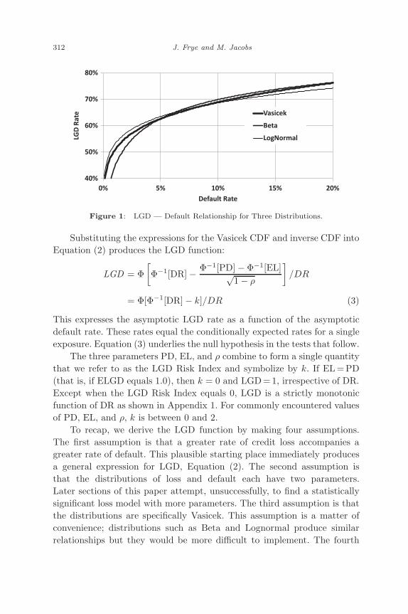
When e = ρ, Equation (14) becomes identical to Equation (3). Figure 4illustrates this when e takes the value 14.51%. Relative to that, greatervalues of e make the function steeper and lesser values of e make thefunction flatter or negatively sloped. For any value of e, the mathematicalexpectation of loss equals the mean of the Vasicek loss distribution, whichis parameter EL.
This section introduces four alternative LGD models. Each alternativecontains an extra parameter that can allow LGD to be more (or less)sensitive to DR than the null hypothesis. The additional parameter hasno effect on the expectation of loss. Therefore, the alternatives focus solelyon the question of the slope of the LGD-default relationship. Later sectionsuse the alternatives in statistical challenges to Equation (3).

November 19, 2012 8:58 9in x 6in Measuring and Managing of Risk b1485-ch11 2nd Reading
Credit Loss and Systematic LGD 323
40%
50%
60%
70%
80%
90%
0% 5% 10% 15% 20%
LGD
Rat
e
Default Rate
e = 19%
e = 14.51% (H0)
e = 10%
Figure 4: Alternative E for Three Values of e.
Testing Cells Separately
This section performs tests on the twenty five cells one cell at a time. Eachcell isolates a particular Moody’s rating and a particular seniority. Each testcalibrates Equation (8) twice: once using Equation (3) and once using analternative LGD function. The likelihood ratio statistic determines whetherthe alternative produces a significant improvement. Judged as a whole, theresults to be presented are consistent with the idea that Equation (3) doesnot misstate the relationship between LGD and default.
As with most studies that use the likelihood ratio, it is compared toa distribution that assumes an essentially infinite, “asymptotic” data set.The statistic itself, however, is computed from a sample of only twenty-sevenyears of data. This gives the statistic a degree of sampling variation that itwould not have in the theoretical asymptotic data. As a consequence, tailobservations tend to be encountered more often than they should be. Thiscreates a bias toward finding statistical significance. This bias strengthensa finding of no significance, such as produced here.
Most risk managers are currently unable to calibrate all the parametersof a loss model by maximum likelihood estimation (MLE). A scientificfinding that is valid only when MLE is employed would be useless tothem. Instead, we calibrate mean parameters along the lines followed bypractitioners. Our estimator for PD in a cell is the commonly-used averageannual default rate. Our estimator for EL is the average annual loss rate.ELGD is the ratio of EL to PD.
In the case of ρ, we find MLE to be more convenient than otherestimators. (The next section checks the sensitivity of test results to the
November 19, 2012 8:58 9in x 6in Measuring and Managing of Risk b1485-ch11 2nd Reading
324 J. Frye and M. Jacobs
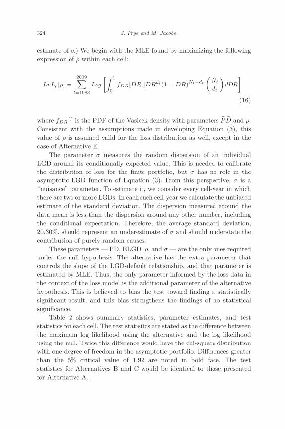
estimate of ρ.) We begin with the MLE found by maximizing the followingexpression of ρ within each cell:
LnLρ[ρ] =2009∑
t=1983
Log[∫ 1
0
fDR[DRt]DRdt(1 − DR)Nt−dt
(Nt
dt
)dDR
]
(16)
where fDR[·] is the PDF of the Vasicek density with parameters PD and ρ.Consistent with the assumptions made in developing Equation (3), thisvalue of ρ is assumed valid for the loss distribution as well, except in thecase of Alternative E.
The parameter σ measures the random dispersion of an individualLGD around its conditionally expected value. This is needed to calibratethe distribution of loss for the finite portfolio, but σ has no role in theasymptotic LGD function of Equation (3). From this perspective, σ is a“nuisance” parameter. To estimate it, we consider every cell-year in whichthere are two or more LGDs. In each such cell-year we calculate the unbiasedestimate of the standard deviation. The dispersion measured around thedata mean is less than the dispersion around any other number, includingthe conditional expectation. Therefore, the average standard deviation,20.30%, should represent an underestimate of σ and should understate thecontribution of purely random causes.
These parameters — PD, ELGD, ρ, and σ — are the only ones requiredunder the null hypothesis. The alternative has the extra parameter thatcontrols the slope of the LGD-default relationship, and that parameter isestimated by MLE. Thus, the only parameter informed by the loss data inthe context of the loss model is the additional parameter of the alternativehypothesis. This is believed to bias the test toward finding a statisticallysignificant result, and this bias strengthens the findings of no statisticalsignificance.
Table 2 shows summary statistics, parameter estimates, and teststatistics for each cell. The test statistics are stated as the difference betweenthe maximum log likelihood using the alternative and the log likelihoodusing the null. Twice this difference would have the chi-square distributionwith one degree of freedom in the asymptotic portfolio. Differences greaterthan the 5% critical value of 1.92 are noted in bold face. The teststatistics for Alternatives B and C would be identical to those presentedfor Alternative A.

November 19, 2012 8:58 9in x 6in Measuring and Managing of Risk b1485-ch11 2nd Reading
Credit Loss and Systematic LGD 325
Table
2:
Basi
cSta
tist
ics,
Para
met
er,E
stim
ate
s,and
Tes
tSta
tist
ics
by
Cel
l.
Senio
rSenio
rSenio
rSenio
rSubord
inate
d
Secure
dLoans
Secure
dB
onds
Unse
cure
dB
onds
Subord
inate
dB
onds
Bonds
Avera
ges
Ba3
EL
D0.2
%4
0.7
%3
0.4
%6
0.8
%9
0.9
%26
0.6
%10
PD
N0.6
%616
2.1
%179
0.8
%703
1.2
%525
1.5
%874
1.1
%579
ELG
DD
Years
42%
333%
349%
463%
664%
855%
5
ρN
Years
7.6
%14
1.0
%26
27.5
%27
5.6
%26
7.9
%21
11.8
%23
Film
PD
Film
D0.7
%5
2.1
%3
1.2
%9
1.2
%9
1.7
%31
1.3
%11
a∆
LnL
−9.0
00.3
71.4
50.0
12.0
70.1
74.7
50.4
71.1
60.0
50.0
90.2
1
e∆
LnL
20.4
%0.4
91.0
%0.0
011.9
%0.2
32.8
%0.4
37.1
%0.0
48.6
%0.2
4
B1
EL
D0.2
%9
0.2
%2
1.0
%13
1.4
%22
1.3
%38
0.8
%17
PD
N0.8
%1332
0.6
%205
1.8
%757
1.9
%909
2.5
%756
1.5
%792
ELG
DD
Years
28%
529%
253%
10
74%
10
51%
10
54%
7
ρN
Years
14.4
%14
1.0
%27
1.0
%27
5.2
%25
8.8
%25
7.9
%24
Film
PD
Film
D1.8
%25
0.8
%3
2.3
%17
2.0
%24
3.0
%45
2.1
%23
a∆
LnL
0.8
20.0
4−
5.4
60.0
0−
14.2
80.2
91.8
90.0
7−
0.3
60.0
1−
3.4
80.0
8
e∆
LnL
12.3
%0.0
22.3
%0.0
03.4
%0.2
94.4
%0.0
79.8
%0.0
26.5
%0.0
8
B2
EL
D0.4
%24
2.5
%4
2.5
%45
2.1
%36
3.2
%35
1.5
%29
PD
N1.2
%1842
5.8
%168
4.1
%826
3.0
%740
5.7
%325
2.8
%780
ELG
DD
Years
36%
10
43%
460%
14
69%
857%
11
55%
9
ρN
Years
5.0
%14
56.9
%26
11.6
%27
8.3
%21
12.1
%26
9.9
%23
Film
PD
Film
D3.0
%61
6.1
%5
4.9
%51
3.2
%40
6.1
%39
3.8
%39
a∆
LnL
−1.8
00.1
11.7
61.1
7−
2.3
50.5
01.2
40.0
5−
0.6
80.0
4−
0.3
70.3
8
e∆
LnL
6.9
%0.1
129.6
%1.0
716.5
%0.6
87.4
%0.0
313.8
%0.0
414.9
%0.3
9
B3
EL
D0.4
%19
2.9
%11
3.5
%45
4.2
%33
6.5
%58
2.6
%33
PD
N1.4
%1374
7.3
%218
6.7
%813
10.5
%382
10.1
%371
5.3
%632
ELG
DD
Years
29%
640%
852%
17
40%
14
64%
13
48%
12
ρN
Years
21.3
%14
38.3
%26
13.9
%27
9.4
%22
11.7
%21
18.0
%22
Film
PD
Film
D4.1
%47
8.1
%13
8.5
%58
10.9
%36
12.0
%73
7.3
%45
a∆
LnL
3.5
62.5
42.5
51.4
0−
0.5
80.0
7−
2.7
21.0
80.8
10.1
50.7
31.0
5
e∆
LnL
3.1
%2.4
09.7
%1.2
315.7
%0.0
818.3
%1.1
89.9
%0.1
411.4
%1.0
1
(Continued
)

November 19, 2012 8:58 9in x 6in Measuring and Managing of Risk b1485-ch11 2nd Reading
326 J. Frye and M. Jacobs
Table
2:
(Continued
)
Senio
rSenio
rSenio
rSenio
rSubord
inate
d
Secure
dLoans
Secure
dB
onds
Unse
cure
dB
onds
Subord
inate
dB
onds
Bonds
Avera
ges
CEL
D2.1
%88
5.1
%49
6.9
%125
19.0
%58
4.2
%12
6.0
%66
PD
N5.6
%956
9.8
%449
11.5
%914
25.1
%288
5.8
%183
10.2
%558
ELG
DD
Years
38%
10
52%
17
60%
21
76%
14
73%
659%
14
ρN
Years
16.9
%14
12.3
%27
6.2
%27
16.4
%16
11.2
%19
12.9
%21
Film
PD
Film
D23.2
%178
13.2
%62
14.3
%149
27.7
%68
10.0
%18
18.3
%95
a∆
LnL
−1.2
60.3
5−
1.4
90.3
80.0
10.0
0−
6.5
82.7
80.9
90.0
3−
1.6
60.7
1
e∆
LnL
23.3
%0.4
717.5
%0.5
18.1
%0.0
031.1
%3.2
010.1
%0.0
218.0
%0.8
4
Avera
ges
EL
D0.6
%29
2.9
%14
3.0
%47
3.6
%32
2.4
%34
2.1
%31
PD
N1.8
%1224
6.1
%244
5.3
%803
5.6
%569
3.9
%502
3.9
%668
ELG
DD
Years
35%
747%
757%
13
65%
10
61%
10
55%
9
ρN
Years
12.8
%14
19.5
%26
12.1
%27
7.8
%22
9.5
%22
11.8
%22
Film
PD
Film
D5.9
%63.2
7.6
%17.2
6.6
%56.8
6.0
%35.4
4.8
%41.2
6.1
%43
a∆
LnL
−1.5
30.6
8−
0.2
40.5
9−
3.0
30.2
1−
0.2
80.8
90.3
90.0
6−
0.9
40.4
9
e∆
LnL
13.2
%0.7
012.0
%0.5
611.1
%0.2
612.8
%0.9
810.1
%0.0
511.9
%0.5
1
Key
toTable
2:
EL,P
D,and
ρ:E
stim
ate
sas
dis
cuss
edin
the
text;
ELG
D=
EL/P
D.
D:T
he
num
ber
ofdef
aults
inth
ece
ll,co
unti
ng
wit
hin
all
27
yea
rs.
N:T
he
num
ber
offirm
-yea
rsofex
posu
rein
the
cell,co
unti
ng
wit
hin
all
27
yea
rs.
DYea
rs:T
he
num
ber
ofyea
rsth
at
hav
eat
least
one
def
ault.
NYea
rs:T
he
num
ber
ofyea
rsth
at
hav
eat
least
one
firm
expose
d.
Nom
D:T
he
num
ber
ofnom
inaldef
aults
(incl
udin
gw
her
eth
ere
sultin
glo
ssis
unknow
n).
Nom
PD
:A
ver
age
ofannualnom
inaldef
ault
rate
s.a,e:
MLE
softh
epara
met
ers
inA
lter
nati
ves
Aand
E.
∆LnL:th
epic
k-u
ps
inLnL
Loss
pro
vid
edby
Alter
native
Aor
Ere
lative
toth
enull
hypoth
esis
.Sta
tist
icalsi
gnifi
cance
at
the
5%
level
isin
dic
ate
din
bold
.A
long
the
right
and
bott
om
marg
ins,
aver
age
EL,P
D,and
ρare
wei
ghte
dby
N;oth
erav
erages
are
unw
eighte
d.

November 19, 2012 8:58 9in x 6in Measuring and Managing of Risk b1485-ch11 2nd Reading
Credit Loss and Systematic LGD 327
Along the bottom and on the right of Table 2 are averages. The overallaverages at the bottom right corner contain the most important fact aboutcredit data: they are few in number. The average cell has only 31 defaults,which is about one per year. Since defaults cluster in time, the average cellhas defaults in only 9 years, and only these years can shed light on theconnection between LGD and default.
Not only are the data few in number, they have a low signal-to-noiseratio: the random variation of LGD, measured by σ = 20.30%, is materialcompared to the magnitude of the systematic effect and the number ofLGDs that are observed. A data set such as used here, spanning manyyears with many LGDs, provides the best opportunity to see through therandomness and to characterize the degree of systematic LGD risk.
In Table 2, there are two cells with log likelihood pickups greater than1.92: Loans to B2-rated firms and Senior Subordinated Bonds issued byC-rated firms. This does not signal statistical significance because manytests are being performed. If twenty-five independent tests are conducted,and if each hasa size of 5%, then two or more nominally significant resultswould occur with probability 36%. Of the two or more nominally significantresults, one cell is estimated steeper than Equation (3) and one cell isestimated flatter than Equation (3). Nothing about this pattern suggeststhat the LGD function of Equation (3) is either too steep or too flat.
Considering all twenty-five cells including the twenty-three cells thatlack nominal significance, there is about a 50-50 split. About half thecells have an estimated LGD function that is steeper than Equation (3)and about half have an estimated LGD function that is flatter thanEquation (3). A pattern like this would be expected if the null hypothesiswere correct.
Summarizing, this section performs statistical tests of the null hypoth-esis one cell at a time. Two cells produce nominal significance, which is anexpected result if the null hypothesis were correct. Of the two cells, onecell has an estimated LGD function that is steeper than the null hypothesisand the other cell has an estimated LGD function that is flatter than thenull hypothesis. Of the statistically insignificant results, about half the cellshave an estimated LGD function that is steeper than the null hypothesisand the other half have an estimated LGD function that is flatter than thenull hypothesis. The pattern of results is of the type to be expected whenthe null hypothesis is correct. This section provides no good evidence thatEquation (3) either overstates or understates LGD risk.

November 19, 2012 8:58 9in x 6in Measuring and Managing of Risk b1485-ch11 2nd Reading
328 J. Frye and M. Jacobs
Testing Cells in Parallel
This section tests using several cells at once. To coordinate the creditcycle across cells, we assume that the conditional rates are connected bya comonotonic copula. Operationally, the conditional rate in every celldepends on a single risk factor. All cells therefore provide information aboutthe state of this factor.
We begin by analyzing the five cells of loans taken together. There are6,120 firm-years of exposure in all. The cell-specific estimates of EL andPD are equal to those appearing in Table 1. The average of the standarddeviation of loan LGD provides the estimate σ = 23.3%. We estimate ρ =18.5% by maximizing the following likelihood in ρ:
LnLρ =2009∑
t=1996
Log
∫ 1
0
5∏i=1
(Φ−1[PDi] +
√ρΦ−1[q]√
1 − ρ
)dt,i
×(
1 − Φ−1[PDi] +√
ρΦ−1[q]√1 − ρ
)Nt,i−dt,i (Nt,i
dt,i
)dq
(17)
The top section of Table 3 shows the estimates of the parameters andpickups of LnL that result. The estimates of a , b, c and e suggest steepnessthat is slightly less than the null hypothesis, but none of the alternativescomes close to the statistically significant pickup of ∆LnL > 1.92. For thefive cells of loans taken together, the null hypothesis survives testing byeach of the four alternatives.
Turning to the twenty cells of bonds, some firms have bonds outstandingin different seniority classes in the same year. Of the total of 10,585firm-years of bond exposure, 9.0% have exposure in two seniority classes,0.4% have exposure in three classes, and 0.1% have exposure in all fourclasses. This creates an intricate dependence between cells rather thanindependence. Assuming that this degree of dependence does not invalidatethe main result, the middle section of Table 3 shows parameter valuessuggesting steepness slightly greater than the null hypothesis. Again, noneof the alternative models come close to statistical significance and the nullhypothesis survives testing.
When all loans and bonds are considered together, 16.0% of firm-years have exposure to two or more classes. Analyzing these simultaneouslyproduces the parameter estimates in the bottom section of Table 3. Once

November 19, 2012 8:58 9in x 6in Measuring and Managing of Risk b1485-ch11 2nd Reading
Credit Loss and Systematic LGD 329
Table 3: Testing Cells in Parallel.
Parameter Estimate ∆ LnL
Loans only; σ = 23.3%, ρ = 18.5%a 0.01 0.00b 0.19 0.31c 0.11 0.19e 0.158 0.28
Bonds only; σ = 19.7%, ρ = 8.05%a −0.43 0.28b −0.03 0.03c −0.03 0.06e 0.085 0.10
Loans and bonds; σ = 20.3%, ρ = 9.01%a −0.81 1.28b −0.10 0.41c −0.09 0.55e 0.102 0.76
again, the alternative models remain far from statistically significant andthe null hypothesis survives testing.
The foregoing tests use maximum likelihood estimates of ρ. Riskmanagers take estimates of ρ from various sources. These include vendedmodels, asset or equity return correlations, credit default swaps, regulatoryauthorities, and inferences from academic studies. All of these sources arepresumably intended to produce an estimate of the statistical parameterthat appears in a Vasicek Distribution relevant for an asymptotic portfolio.4
Still, it is natural to ask whether a different value of ρ would lead toa different conclusion about the statistical significance of the alternativehypotheses.
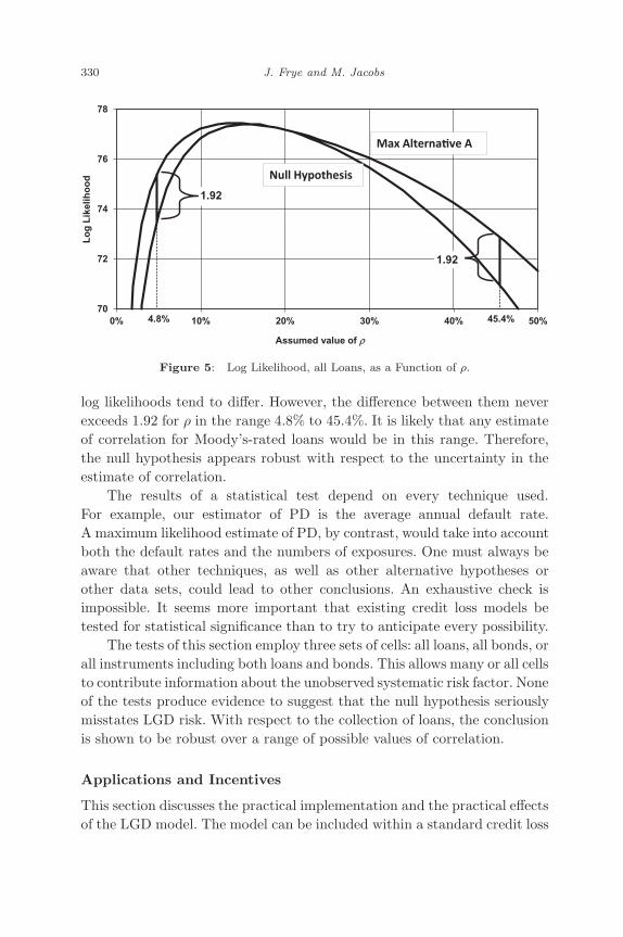
To investigate this, we repeat the analysis of Table 3 for the collectionof Loan cells. In each repetition, we assume a value of ρ. Based onthat, we calculate the log likelihood under the null hypothesis and underAlternative A. A significant result would be indicated by a difference in loglikelihoods greater than 1.92.
Figure 5 displays the results. The lower line is the log likelihood of lossunder the null hypothesis, and the upper line is the maximum log likelihoodof loss under Alternative A. When ρ equals 18.5% the two are nearlyequal, as already shown in Table 3. When ρ takes different value, the two
4Frye (2008) discusses the difference between the correlation in a statistical distributionand the correlation between asset returns that is often used as an estimator.
November 19, 2012 8:58 9in x 6in Measuring and Managing of Risk b1485-ch11 2nd Reading
330 J. Frye and M. Jacobs
4.8% 45.4%70
72
74
76
78
0% 10% 20% 30% 40% 50%
Lo
g L
ikel
iho
od
Assumed value of ρ
1.92
1.92
Null Hypothesis
Max Alternative A
Figure 5: Log Likelihood, all Loans, as a Function of ρ.
log likelihoods tend to differ. However, the difference between them neverexceeds 1.92 for ρ in the range 4.8% to 45.4%. It is likely that any estimateof correlation for Moody’s-rated loans would be in this range. Therefore,the null hypothesis appears robust with respect to the uncertainty in theestimate of correlation.
The results of a statistical test depend on every technique used.For example, our estimator of PD is the average annual default rate.A maximum likelihood estimate of PD, by contrast, would take into accountboth the default rates and the numbers of exposures. One must always beaware that other techniques, as well as other alternative hypotheses orother data sets, could lead to other conclusions. An exhaustive check isimpossible. It seems more important that existing credit loss models betested for statistical significance than to try to anticipate every possibility.
The tests of this section employ three sets of cells: all loans, all bonds, orall instruments including both loans and bonds. This allows many or all cellsto contribute information about the unobserved systematic risk factor. Noneof the tests produce evidence to suggest that the null hypothesis seriouslymisstates LGD risk. With respect to the collection of loans, the conclusionis shown to be robust over a range of possible values of correlation.
Applications and Incentives
This section discusses the practical implementation and the practical effectsof the LGD model. The model can be included within a standard credit loss

November 19, 2012 8:58 9in x 6in Measuring and Managing of Risk b1485-ch11 2nd Reading
Credit Loss and Systematic LGD 331
model without much difficulty. Outside the model, it can be used to obtainscenario-specific LGDs. If the LGD model were used to establish the capitalcharges associated to new credit exposures, new incentives would result.
A standard credit loss model could use Equation (3) to determine con-ditionally expected LGD. Estimates of parameters PD and EL (or ELGD)are already part of the credit model. The value of ρ has little impact on theLGD-default relationship. A practical estimator of ρ might be a weightedaverage of an exposure’s correlations with other exposures.
Some credit loss models work directly with unobserved factors thatestablish the conditional expectations, and these models would have DRreadily available. Other credit models have available only the simulateddefault rate. Each simulation run, these models could place the portfoliodefault rate within a percentile of its distribution, and use that percentile toestimate the DR of each defaulted exposure in the simulation run. An LGDwould be drawn from a distribution centered at the conditionally expectedrate. This approximation is expected to produce reasonable results for thesimulated distribution of loss. Every exposure would have LGD risk, andportfolio LGD would be relatively high in simulation runs where the defaultrate is relatively high.
Outside a credit loss model, risk managers might want to have anestimate of expected LGD under particular scenarios. One importantscenario is that DR has a tail realization. In a tail event, there would bemany defaults, and individual LGDs should average out quite close to theconditionally expected LGD rate.
In the bad tail, conditionally expected LGD is greater than ELGD.Figure 6 shows the difference at the 99.9th percentile. Functions for sixdifferent exposures are illustrated. Based on its PD, each exposure hasρ taken from the Basel II formula.
An exposure with PD=10% is illustrated on the top line. If ELGD wereequal to 10%, LGD in the 99.9th percentile would equal (10% +12%) =22%, which is more than twice the value of ELGD. If ELGD were equalto 20%, LGD in the 99.9th percentile would equal (20% + 16%) = 36%.The diagram makes clear that the LGD function extracts a premiumfrom exposures having the low-ELGD, High-PD combination. Relative tosystems that ignore LGD risk, this relatively discourages exposures thathave exhibited low historical LGD rates and relatively favors exposuresthat have low PD rates.
In Figure 6, the conditional LGD rate depends on both parameters —PD and ELGD. That traces back to the derivation of the LGD function.

November 19, 2012 8:58 9in x 6in Measuring and Managing of Risk b1485-ch11 2nd Reading
332 J. Frye and M. Jacobs
0%
2%
4%
6%
8%
10%
12%
14%
16%
18%
20%
0% 20% 40% 60% 80% 100%
LG
D A
dd
-on
ELGD
PD = 10%, Rho = 12.1%PD = 3%, Rho = 14.7%PD = 1%, Rho = 19.3%PD = 0.3%, Rho = 22.3%PD = 0.1%, Rho = 23.4%PD = 0.03%, Rho = 23.8%
Figure 6: 99.9th Percentile LGD Less ELGD.
If the LGD function had no sensitivity to PD, the credit loss distributionwould have three parameters rather than two. Thus, the idea that thedistribution of credit loss can be seen only two parameters deep withexisting data has a very practical risk management implication.
If this approach to LGD were used to set capital charges for extensionsof credit, new incentives would result. The asymptotic loss distributionhas two parameters, EL and ρ. Assuming that the parameter ρ is uniformacross a set of exposures, two credit exposures having the same EL wouldhave the same credit risk. The capital attributed to any exposure would beprimarily a function of its EL. EL, rather than the breakdown of EL intoPD and ELGD, would become the primary focus of risk managers. Thiswould produce an operational efficiency and also serve the more generalgoals of credit risk management.
Conclusion
If credit loss researchers had thousands of years of data, they might possessa detailed understanding of the relationship between the LGD rate andthe default rate. However, only a few dozen years of data exist. Logically,it is possible that these data are too scanty to allow careful researchersto distinguish between theories. This possibility motivates the currentpaper.
This study begins with simple statistical models of credit loss anddefault and infers LGD as a function of the default rate. Using a long
November 19, 2012 8:58 9in x 6in Measuring and Managing of Risk b1485-ch11 2nd Reading
Credit Loss and Systematic LGD 333
and carefully observed data set, this function is tested but it is not foundto be too steep or too shallow. It produces greater LGD rates with greaterdefault rates. It uses only parameters that are already part of credit lossmodels; therefore, the LGD function can be implemented as it is. It can alsobe subject to further testing. By far, the most important tests would beagainst the portfolio credit loss models now running at financial institutions.If those models do not have statistical significance against Equation (3),they should be modified to improve their handling of systematic LGDrisk.
Appendix 1: Analysis of the LGD Function
Appendix 1 analyzes Equation (3). It can be restated using the substitutionEL =PD ELGD:
LGD = Φ[Φ−1[DR] − Φ−1[PD] − Φ−1[PDELGD]√
1 − ρ
]/DR (18)
The parameters combine to form a single value that we symbolize by k:
k =Φ−1[PD] − Φ−1[PDELGD]√
1 − ρ; LGD = Φ[Φ−1[DR] − k]/DR (19)
LGD functions differ from each other only because their parameter valuesproduce different values of k. We refer to k as the LGD Risk Index.
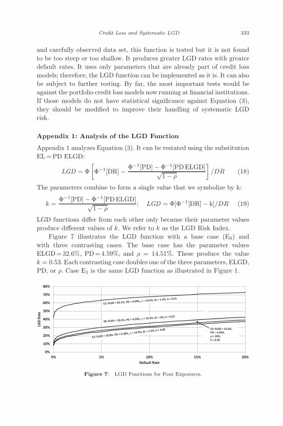
Figure 7 illustrates the LGD function with a base case (E0) andwith three contrasting cases. The base case has the parameter valuesELGD=32.6%, PD=4.59%, and ρ = 14.51%. These produce the valuek = 0.53. Each contrasting case doubles one of the three parameters, ELGD,PD, or ρ. Case E1 is the same LGD function as illustrated in Figure 1.
0%
10%
20%
30%
40%
50%
60%
70%
80%
0% 5% 10% 15% 20%
LGD
Rat
e
Default Rate
E3: ELGD = 32.6%, PD = 4.59%, ρ = 29%, k = 0.58
Figure 7: LGD Functions for Four Exposures.

November 19, 2012 8:58 9in x 6in Measuring and Managing of Risk b1485-ch11 2nd Reading
334 J. Frye and M. Jacobs
Along each LGD function, LGD rises moderately with default. In theirnearly linear regions from 5% to 15%, LGD rises by slightly less than 10%for each of the illustrated exposures.
LGD lines cannot cross, because the LGD Risk Index k acts similarto a shift factor. Comparing the three contrasting cases, E1 is the mostdistant from E0. That is because the unconditional expectation, ELGD,has the most effect on k; not surprisingly, ELGD is the most importantvariable affecting the conditional expectation, LGD. Next most importantis PD, which has partially offsetting influences on the numerator of k. Leastimportant is the value of ρ. This is useful to know because the value of ρ
might be known within limits that are tight enough — say, 5%–25% forcorporate credit exposures — to put tight bounds on the influence of ρ.
In general, an estimate of PD tends to be close to the average annualdefault rate. (Our estimator of PD is in fact exactly equal to the averageannual default rate.) An estimate of ELGD, however, tends to be greaterthan the average annual LGD rate. The latter is sometimes referred to as“time-weighted” LGD, since it weights equally the portfolio average LGDsthat are produced at different times. By contrast, an estimate of ELGDis “default-rate-weighted.” This tends to be greater than the time-weightedaverage, because it places greater weight on the times when the defaultrate is elevated, and these tend to be times when the LGD rate is elevated.As a consequence, the point (PD, ELGD) tends to appear above the middleof a data swarm.
The LGD function passes close to the point (PD, ELGD). This can beseen by inspection of Equation (17). In the unrealistic but mathematicallypermitted case that ρ = 0, if DR = PD then LGD=ELGD. In other words,if ρ = 0 the LGD function passes exactly through the point (PD, ELGD).In the realistic case that ρ > 0, the LGD function passes lower than this. InFigure 7, Function E1 passes through (4.59%, 62.9%), which is 2.3% lowerthan (PD= 4.59%, ELGD=65.1%). Function E2 passes through (9.18%,29.4%), which is 3.2% lower than (PD= 9.18%, ELGD= 32.6%).
For a given combination of PD and ELGD, the “drop” — the verticaldifference between the point (PD, ELGD) and the function value — dependson ρ; greater ρ produces greater drop. (On the other hand, greater ρ allowsthe data to disperse further along the LGD function. This is the mechanismthat keeps EL invariant when ρ becomes greater.) The amount of the dropcan be placed within limits that are easy to calculate. If ρ takes the valueof 25%, the drop is 4%–7% for all PD less than 50% and all ELGD between10% and 70%. If ρ takes the value of 4%, the drop is less than 1% for

November 19, 2012 8:58 9in x 6in Measuring and Managing of Risk b1485-ch11 2nd Reading
Credit Loss and Systematic LGD 335
0.1%
1.0%
10.0%
100.0%
0.1% 1.0% 10.0% 100.0%
LGD
Rat
e
Default Rate
ELGD = 100%, k = 0.0ELGD = 50%, k = 0.34ELGD = 20%, k = 0.74ELGD = 10%, k = 1.01ELGD = 5%, k = 1.26ELGD = 2%, k = 1.57ELGD = 1%, k = 1.78
Figure 8: LGD Functions: PD=5%, ρ = 15%, and Seven Values of ELGD.
all PD and all ELGD. For all values of parameters that are likely to beencountered, the LGD function tends to pass slightly lower than the point(PD, ELGD).
The LGD function of Equation (3) is strictly monotonic. Figure 8illustrates this for seven exposures that share a common value of PD (5%)and a common value of ρ (15%), but differ widely in ELGD.
Because both the axes of Figure 8 are on a logarithmic scale, theslopes of lines in Figure 8 can be interpreted as elasticities, which measureresponsiveness in percentage terms. The elasticity of LGD with respect toDR is defined as
ηDRLGD =∂LGD∂DR
DR
LGD(20)
Looking in the range 1%<DR < 10%, the slope is greater for lines that arelower; that is, the elasticity of LGD with respect to DR is high when ELGDis low. Thus, when default rates rise the biggest percentage changes in LGDare likely to be seen in low-ELGD exposures.
Figure 8 represents by extension the entire range of LGD functions thatcan arise. Each of the LGD functions illustrated in Figure 8 could apply toinfinitely many other exposures that have parameters implying the samevalue of k.
Appendix 2: Alternative A and Pykhtin’s LGD Model
A solid theoretical model of LGD is provided by Michael Pykhtin. ThisAppendix discusses Pykhtin’s model and then illustrates that Alternative Ais similar to it. In fact, Alternative A can be thought of as an approximationto Pykhtin’s model, if the slopes are low or moderate. Therefore, although

November 19, 2012 8:58 9in x 6in Measuring and Managing of Risk b1485-ch11 2nd Reading
336 J. Frye and M. Jacobs
we do not test directly against Pykhtin’s model, this suggests that we testagainst an alternative that is very much like it.
Pykhtin’s LGD model depends on a single factor that can be the sameone that gives rise to variation of the default rate. Adapting Pykhtin’soriginal notation and reversing the dependence on Z, there are threeparameters that control the relationship between LGDPyk and the standardnormal factor Z:
LGDPyk = Φ
[−µ
σ+ ρLGDZ√
1 − ρ2LGD
]− Exp
[µ + σ2(1 − ρLGD)
2− σρLGDZ
]
×Φ
[−µ
σ+ ρLGDZ − σ(1 − ρ2
LGD)√1 − ρ2
LGD
](21)
Pykhtin’s three parameters are µ, σ, and ρLGD. Roughly stated, thesemeasure the log of the initial value of collateral, the dispersion of itsending value, and the correlation between its return and the risk factorZ. Obviously, this is a model of the dynamics of collateral; LGD isdetermined as the outcome of those dynamics. If there is very littlecollateral, LGD takes a high value and there is very little for the modelto do. Thus, the contribution of the model is most apparent when ELGD islow.
Pykhtin’s LGD model can be combined with Vasicek’s default model,which relates the rate of default to the unobserved risk factor Z:
DR = Φ[Φ−1[PD] +
√ρZ√
1 − ρ
]; Z =
√1 − ρΦ−1[DR] − Φ−1[PD]√
ρ(22)
The expression for Z can be substituted into Equation (20) to producea relationship between LGD and default. In this relationship, LGD is amonotonic increasing function of DR that approaches the limits of zeroand one as DR approaches the same limits.
Pykhtin’s LGD model could be used to test the null hypothesis ofEquation (3). To produce the correct value of EL, the parameter valuesmust obey the following restriction:
EL =∫ ∞
−∞LGDPyk[z]DR[z]φ[z]dz (23)
Maximizing Equation (9) using LGD function of Equation (20) and subjectto the constraint expressed by Equation (22) is believed to require asubstantial commitment to numerical optimization of what is apt to be
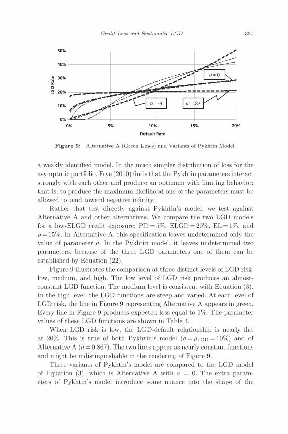
November 19, 2012 8:58 9in x 6in Measuring and Managing of Risk b1485-ch11 2nd Reading
Credit Loss and Systematic LGD 337
0%
10%
20%
30%
40%
50%
0% 5% 10% 15% 20%
LGD
Rat
e
Default Rate
a = .87a = -3
a = 0
Figure 9: Alternative A (Green Lines) and Variants of Pykhtin Model.
a weakly identified model. In the much simpler distribution of loss for theasymptotic portfolio, Frye (2010) finds that the Pykhtin parameters interactstrongly with each other and produce an optimum with limiting behavior;that is, to produce the maximum likelihood one of the parameters must beallowed to tend toward negative infinity.
Rather that test directly against Pykhtin’s model, we test againstAlternative A and other alternatives. We compare the two LGD modelsfor a low-ELGD credit exposure: PD= 5%, ELGD= 20%, EL =1%, andρ =15%. In Alternative A, this specification leaves undetermined only thevalue of parameter a. In the Pykhtin model, it leaves undetermined twoparameters, because of the three LGD parameters one of them can beestablished by Equation (22).
Figure 9 illustrates the comparison at three distinct levels of LGD risk:low, medium, and high. The low level of LGD risk produces an almost-constant LGD function. The medium level is consistent with Equation (3).In the high level, the LGD functions are steep and varied. At each level ofLGD risk, the line in Figure 9 representing Alternative A appears in green.Every line in Figure 9 produces expected loss equal to 1%. The parametervalues of these LGD functions are shown in Table 4.
When LGD risk is low, the LGD-default relationship is nearly flatat 20%. This is true of both Pykhtin’s model (σ = ρLGD =10%) and ofAlternative A (a =0.867). The two lines appear as nearly constant functionsand might be indistinguishable in the rendering of Figure 9.
Three variants of Pykhtin’s model are compared to the LGD modelof Equation (3), which is Alternative A with a = 0. The extra param-eters of Pykhtin’s model introduce some nuance into the shape of the

November 19, 2012 8:58 9in x 6in Measuring and Managing of Risk b1485-ch11 2nd Reading
338 J. Frye and M. Jacobs
Table 4: LGD Functions in Figure 9.
Pykhtin ModelAlternative Aa µ σ ρLGD
Low LGD risk0.867 −0.220 0.100 0.100
Medium LGD risk
0.000 −0.119 0.320 0.320(null hypothesis) 0.294 0.950 0.230
−0.169 0.075 0.950
High LGD risk
−3.000 0.256 0.640 0.6400.550 0.950 0.590
−0.044 0.235 0.950
relationship, but not much. Two of the variants of Pykhtin’s modelinvolve large parameter values (either σ or ρLGD equals 95%), and thethird one involves equal values (σ = ρLGD =32%). Despite diverse sets ofparameter values, the LGD functions are nearly the same except at the left,where LGD functions are particularly difficult to distinguish by empiricaldata.
Comparing to the high-risk case when parameter a equals –3, thenuance of Pykhtin’s model is clear. Economically, the borrower postsconsiderable collateral (µ is elevated), but the collateral is subject to bothgreat systematic risk and to great idiosyncratic risk. The shapes producedby the Pykhtin model are different from the shape of Alternative A andsomewhat different from each other; the one with ρLGD equal to 95% isdistinct from the other two. If the slope of the LGD function were foundto be this steep, the nuance provided by the Pykhtin model might make asignificant contribution relative to Alternative A.
To summarize this illustration, Alternative A is a close approximationof the Pykhtin model when LGD risk is low or moderate, but the twomodels differ when LGD risk is high. Since the level of LGD appearingin the Moody’s data appears to be moderate — the null hypothesis,Alternative A with a =0, is not rejected by the tests — we believe thatwe have tested the LGD function against an alternative that is verymuch like Pykhtin’s model. We do not claim that we have shown thatPykhtin’s model would demonstrate a lack of statistical significance ifthe LGD function were tested against it. That test is left for futureresearch.

November 19, 2012 8:58 9in x 6in Measuring and Managing of Risk b1485-ch11 2nd Reading
Credit Loss and Systematic LGD 339
References
Altman, EI and B Karlin (2010). Special report on defaults and returns in thehigh-yield bond and distressed debt market: The year 2009 in review andoutlook, NYU Solomon Center Report, February.
Frye, J (2000). Depressing recoveries. Risk, pp. 108–111.———, (2008). Correlation and asset correlation in the structural portfolio model.
Journal of Credit Risk, 4(2), POG. 75–96.———, (2010). Modest means, Risk, pp. 94–98 (January).Gordy, M (2003). A risk-factor model foundation for ratings-based bank capital
rules. Journal of Financial Intermediation, 12(3), pp. 199–232.Gupton, G, C Finger and M Bhatia (1997). CreditMetricsTM — Technical
Document, Moody’s Corporate Default Rate Service, 2010.Pykhtin, M (2003). Unexpected recovery risk. Risk (August), pp. 74–78.Pykhtin, M and A Dev (2002). Analytical approach to credit risk modeling. Risk,
S26–S32 (March).Vasicek, O (2002). Loan portfolio value. Risk, pp. 160–162.