Embed Size (px)
Citation preview


PRATIBHA: INTERNATIONAL JOURNAL OF SCIENCE,
SPIRITUALITY, BUSINESS AND TECHNOLOGY (IJSSBT)
Pratibha: International Journal of Science, Spirituality, Business and Technology
(IJSSBT) is a research journal published by ShramSadhana Bombay Trust‘s, COLLEGE Of
ENGINEERING & TECHNOLOGY, Bambhori, Jalgaon, MAHARASHTRA STATE, INDIA. College was
founded by FORMER PRESIDENT, GOVT. OF INDIA, Honorable Excellency Sau.
PRATIBHA DEVI SINGH PATIL.
College is awarded as Best Engineering College of Maharashtra State by Engineering Education Foundation, Pune in year 2008-09.
The College has ten full-fledged departments. The Under Graduate programs in 7
courses are accredited by National Board of Accreditation, All India Council for
Technical Education, New Delhi for 5 years with effect from 19/07/2008 vide letter
number NBA/ACCR-414/2004. QMS of the College conforms to ISO 9001:2008 and is
certified by JAAZ under the certificate number: 1017-QMS-0117.The college has been
included in the list of colleges prepared under Section 2(f) of the UGC Act, 1956 vide
letter number F 8-40/2008 (CPP-I) dated May, 2008 and 12(B) vide letter number F. No.
8-40/2008(CPP-I/C) dated September 2010.UG courses permanently affiliated to North
Maharashtra University are: Civil Engineering, Chemical Engineering, Computer
Engineering, Electronics and Telecommunication Engineering, Electrical Engineering,
Mechanical Engineering, Information Technology. Two years Post Graduate courses are
Mechanical Engineering (Machine Design), Civil Engineering (Environmental
Engineering), Computer Engineering (Computer Science and Engineering), Electronics,
Telecommunication(Digital Electronics) and Electrical Engineering (Electrical power
systems). Civil Engineering Department, Mechanical, Biotechnology and Chemical
Engineering Department laboratories are registered for Ph.D. Programs. Spread over 25
Acres, the campus of the college is beautifully located on the bank of river Girna.
The International Journal of Science, Spirituality, Business and Technology
(IJSSBT) is an excellent, intellectual, peer reviewed journal that takes scholarly approach
in creating, developing, integrating, sharing and applying knowledge about all the fields
of study in Engineering, Spirituality, Management and Science for the benefit of
humanity and the profession.
The audience includes researchers, managers, engineers, curriculum designers
administrators as well as developers.

EDITOR(s)-IN-CHIEF
Prof. Dr. K. S. WANI,
M. Tech. (Chem. Tech.), D.B.M., Ph. D.
LMISTE, LMAFST, MOTAI, LMBRSI
Principal,
S.S.B.T.‘s College of Engineering and Technology,
P.B. 94, Bambhori,
Jalgaon-425001 Maharashtra, India
Mobile No. +919422787643
Phone No. (0257) 2258393,
Fax No. (0257) 2258392,
Email id: [email protected]
Prof. Dr. DHEERAJ SHESHRAO DESHMUKH
D,M.E., B.E.(Mechanical), M.Tech. (Heat power engineering)
Ph.D. (Mechanical Engineering)
LMISTE,
Professor and Head,
Department of Mechanical Engineering,
S.S.B.T.‘s, College of Engineering and Technology,
P.B. 94, Bambhori,
Jalgaon-425001, Maharashtra State, India
Mobile No. +91 9822418116
Phone No. (0257) 2258393,
Fax No. (0257) 2258392.
Email id : [email protected]
Web Address : www.ijssbt.org/com

PUBLICATION COMMITTEE
SUHAS M. SHEMBEKAR
Assistant Professor
Electrical Engineering Department
S. S. B. T.‘s College of Engineering and Technology,Bambhori, Jalgaon (M.S.)
DHANESH S. PATIL
Assistant Professor
Electrical Engineering Department
S. S. B. T.‘s College of Engineering and Technology,Bambhori, Jalgaon (M.S.)
LOCAL REVIEW COMMITTE
Dr. K. S. Wani
Principal
S.S.B.T.‘s College of Engineering &
Technology,
Bambhori, Jalgaon
Dr. M. Husain
Professor & Head
Department of Civil Engineering
Dr. I.D. Patil
Professor & Head
Department of Bio-Technology
Dr. M. N. Panigrahi
Professor & Head
Department of Applied Science
Dr. V.R. Diware
Associate Professor& Head
Department of Chemical Engineering
Dr. U. S. Bhadade
Professor & Head
Department of Electronics &
Telecommunication Engineering
Dr. D. S. Deshmukh
Professor & Head
Department of Mechanical Engineering
Dr. G. K. Patnaik
Professor & Head
Department of Computer Engineering
Dr. P. J. Shah
Professor & Head
Department of Electrical Engineering
S. J. Patil
Assistant Professor & Head
Department of Information Technology
Dr. V. S. Rana
Associate Professor & Head
Department

PRATIBHA: INTERNATIONAL JOURNAL OF SCIENCE,
SPIRITUALITY, BUSINESS AND TECHNOLOGY
(IJSSBT) Table of Contents
Volume 3, No. 1, Dec, 2014
Detergent Removal from Sullage by Photo-catalytic Process
……………....……………………………………………………………………….....01 Dr.Kishor S.Wani, Dr. Mujahid Husain and Dr. Vijay R Diware
AUTOMATIC PRODUCT HANDLING, IDENTIFICATION AND SORTING
USING LabVIEW…...………………………………………………………..……....06 Sachin S. Nerkar, Mahesh S. Patil
The study of internet banking Usage: A case study of SBI Dana Bazaar Branch,
Jalgaon…………………………………………………………………………….…..10 Mukesh B. Ahirrao,Pankajkumar A. Anawade, Mangesh Mali
Green HR Practices: An Empirical Study of Cargill, Jalgaon………….…..……14 Dr.VishalS.Rana, Ms.Sonam N.Jain
ANALYSIS OF SPRING BACK DEFECT IN RIGHT ANGLE BENDING
PROCESS IN SHEET METAL FORMING..……..……..………….…….……………18 P.S.NANDANWAR, P.S.BAJAJ, P.D. PATIL
Computational Fluid Dynamics (CFD) Simulation of Helical Coil Induction Water
Heater using Induction Cooker………..……………………………….……………23 Tejas G. Patil, Atul A. Patil, Dheeraj S. Deshmukh
Materials Selection Criteria for Thermoelectric Power Generators Performance
Enhancement: A Critical Review…...…………………………………….………….27 P. M. Solanki, Dr. D.S. Deshmukh
Experimental Verification and CFD Analysis of Single Cylinder Four Strokes C.I.
Engine Exhaust System……………………..……………………………...…...…..33 Atul A. Patil,L.G. Navale,V.S. Patil
IMPROVING EFFICIENCY OF SOLAR WATER HEATER USING PHASE
CHANGE MATERIALS………………………………..………………….…...……39 Mr. M.V. Kulkarni,Dr. D. S Deshmukh
Recent Trends in Banana By-Products and Marketing Strategies: A Critical
Review….……………………………………………………..……………….……….45 Dr.Prashant P. Bornare, Dr.Dheeraj S Deshmukh, Dipak C. Talele
EFFECTS OF GROUNDING SYSTEM ON POWER
QUALITY……………………………………………………………….………….…49 Bhagat Singh Tomar,Dwarka Prasad, ApekshaNarendra Rajput

USE OF RGB COLORS AND CRYPTOGRAPHY FOR COULD SECURITY
……………………………………………………………………….…………...……54 S. J. Patil, N. P. Jagtap ,Shambhu Kumar Singh
Utilization of Cereal Grains for Bioethanol Production: A Critical Review
…………………………………………………………………………….…...……….60 Sheetal B. Gawande, Dr. I. D. Patil
A Critical Review on Low Temperature Solar Water Heater Collectors……...….67 Ashish N. Sarode, Atul A. Patil, Vijay H.Patil
Comparative analysis of Multilayer Perceptron and Radial Basis Function ANN for
prediction of cycle time of Structural subassembly Manufacturing…………...…..71 Jayant P.Giri,Dr. V.H.Tatwawadi, S.G.Mahakalkar, Dr. J.P.Modak
Modeling and Simulation of gate operations of dam for flood management: An
approach……………………………………………………………………………… 83 Pallavi J. Giri , Dr. Ajay R. Gajbhiye
PRATIBHA: INTERNATIONAL JOURNAL OF SCIENCE, SPIRITUALITY,
BUSINESS AND TECHNOLOGY (IJSSBT), Vol. 3, No. 1, Dec 2014
ISSN (Print) 2277—7261
1
Detergent Removal from Sullage by Photo-catalytic Process
Dr.Kishor S.Wani1, Dr.Mujahid Husain
2 and Dr. Vijay R Diware
3*
1. Principal, SSBT‘s College of Engineering & Technology, Bambhori, Jalgaon,MS, India.
2. Professor, Civil Engineering, SSBT‘s College of Engineering & Technology,
Bambhori, Jalgaon, MS, India.
3. *Associate Professor, Chemical Engineering, SSBT‘s College of Engineering & Technology
Bambhori, Jalgaon, MS, India.
Email: [email protected]
*Corresponding author.
Abstract:Photo-catalysis has emerged as a
powerful technological boon to ultimately
decompose and recycle the non-biodegradable
organics. Detergents that are considered to be
stringently non-biodegradable or sparingly
degradable are severe concerns for the
agriculturists as they gradually render the soil
unfit for agriculture. The present research
study has applied photo-catalysis technology to
degrade commercial detergents available in the
sullage (washroom wastewater) of the
residential campus of an engineering college.
The COD (Chemical Oxygen Demand) has been
taken as a parameter for monitoring the
degradation rate of detergent. Photo-catalyst
used is TiO2. The degradation studies are
conducted under artificial source of UV
radiations in an indigenously designed reactor.
Dose of photo-catalyst is varied and optimized.
It has been observed that the COD has been
effectively brought down to the level of 40 mg/L
with an optimal dose of 35 mg/L photo-catalyst.
The sullage is rendered to be fit for gardening
applications. The research outcomes find
significant applications in the recycling of
sullage for gardening and irrigation
applications and will save huge amount of water
and electricity both.
Key words:Photo-catalysis, Detergents, TiO2,
COD.
1. INTRODUCTION
Till 1960s BOD was the most important
parameter of concern in wastewaters [12]. However with the advancement in science and
technology, the synthesis of variety of non-
biodegradable organics has become very common.
They have become integral part of our day to day
life. The concentration of detergents, variety of
cleansers used in households, pesticides, fertilizers,
insecticides, plastic traces, polythene traces etc. is
increasing in wastewaters rapidly. They are non-
biodegradables and are persisting in nature. They
create difficulties in conventional wastewater treatment. They join food chains and accumulate in
human bodies exhibiting long term disorders.
Conventional technologies for removal of non-
biodegradable organics are quite inefficient.
However, photo-catalysis has emerged a powerful
boon for degradation of non-biodegradable
organics [16]. Detergent is one such commonly
used non-biodegradable organics which is
commonly present in domestic wastewaters, and
laundry wastewaters.
With rising population and over
exploitation, the water resources are depleting day by day. There is great need for recycling of water.
Sullage is the wastewater generated from
bathrooms [17]. It is rich in terms of urine but
BOD is not high. It also contains significant
quantity of detergents. At many water scarce
places the sullage is recycled for gardening
applications. However the detergents present in the
sullage affect to the fertility of soil in long term.
Thus they require to be removed. Photo-catalysis
can be applied for removal of detergents from
sullage as well as from various wastewaters. The present work explores the photo-
catalysis technology for treatment of detergent
containing wastewaters. Some parameters of
process are investigated experimentally and
optimized for highest rate of degradation.
1.1 Detergents and their chemistry
In a dictionary detergent is simply defined
as cleaning agent. However, the word detergent
has tended to imply synthetic detergents
specifically, generally termed as surface-active agent or surfactant. The synthetic detergents are
made from petrochemicals [18]. Synthetic
detergents dissolve or tend to dissolve in water or
other solvents. To enable them to do this, they
require distinct chemical characteristics.
Hydrophilic (water loving) groupings in their
molecular structure, and hydrophobic (water
hating) groupings, help the detergent in its
―detergency‖ action. This detergency depends on
PRATIBHA: INTERNATIONAL JOURNAL OF SCIENCE, SPIRITUALITY,
BUSINESS AND TECHNOLOGY (IJSSBT), Vol. 3, No. 1, Dec 2014
ISSN (Print) 2277—7261
2
the balance of the molecular weight of the
hydrophobic to the hydrophilic portion. This is
called the HLB value. There are four main classes
of detergents, anionic, cationic, amphoteric.
1.2 Problems due to detergents in wastewater
Detergents pose a variety of problems in the wastewater treatment. They are surfactants.
Thus they hinder the transfer of oxygen from
atmosphere to the water in the process of aeration.
They reduce the oxygen transfer efficiency to 15%.
They hinder the biological treatment also. They
trap the colloidal particles and keep them on
surface thus reducing the efficiency of coagulation.
Once they find a way in to surface of sub-surface
waters, they join to food chain. They accumulate
in body and exhibit long term disorders like
carcinogenicity, mutagenicity, fertility loss, loss of
potency, allergy etc in long term. During coagulation of water they form halides. The above-
mentioned bad effects are even exaggerated.
1.3 Limitations of Conventional Wastewater
Treatment Technologies in detergent removal
The linear alkyl sulfonates are biodegradable under
aerobic conditions, but not in anaerobic conditions.
The benzyl sulfonates are strongly resistant to
biodegradation. Generally the removal of
detergents from wastewater is favored by methods like adsorption. But these methods simply
transform the problem from one phase to another.
They do not solve the problem. The final disposal
of solid sorbent material containing detergents is
again a problem. From this bulk, detergents may
again find way in to surface and sub-surface
waters.
1.4The photo-catalysis technology
The photo-catalysis is a phenomenon recognized by researchers [5, 6, 9]. Semiconductors have a
property that they emit an electron when light
wave of appropriate wave length fall upon them.
Some of the common conductors are Titanium di
oxide, silicon di oxide, zinc oxide etc. Titanium di
oxide is considered to be the most active. TiO2
emits electron when UV radiation falls on it which
ultimately results into hydroxyl radical formation
[19].
TiO2 + UV = TiO2+ + e
H2O= H+ + OH-
OH- - e +TiO2+ = TiO2 + OH*
OH* + organic compound = products of
mineralization
The UV radiation is obtained from sun or it can be
obtained from UV lamps.
Fujishimaet al [9] first described the reactor design
and process parameter aspects in his bibliographic
work.
1.5 Review of research in photo-catalysis
The process has so many variables listed
as- pH, temperature, intensity of light,
concentration of organic compound, concentration
of catalyst, specific surface area of catalyst etc.
The process is complex and is still in nascent stage
for degradation kinetics modeling. Several
researchers [2, 13, and 14] have used this
technology for removal of VOCs. Brillaset al
(1998) [9] presented a scientific look into the
process and described the electron transfer
phenomenon. Augugliaroet al (1999) and Cao et al
(2000) [4 and 8]applied the process for treatment of toluene in gaseous phase. Alex et al (2003) [3]
used this technology for removal of benzoic acids
using specially designed cascade reactor
configuration. Later researchers showed interest in
the investigations of formation of intermediate
products of the process too Pal et al (2000) [15].
Hakimiet al (2003) [10] applied photo-catalysis
technology for treatment of industrial wastewaters.
Alpert et al (1991) [1] treated hazardous waste
using photo-catalysis. Meng Nan Chong et al
(2010) [11] has presented a review of recent developments in photo-catalysis technology. In
fact the great deal of research going on in the arena
of photo-catalysis can be described by the
bibliography given at the end.
The present work has used the photo-
catalysis technology for removal of detergents
from sullage.
2. MATERIALS AND METHODS
The detergent used for experimental studies is commercial detergent available from the local
market in the brand name of Nirma. It is dissolved
in distilled water to obtain desired concentrations.
The photo-catalyst used is Qualigens grade. The
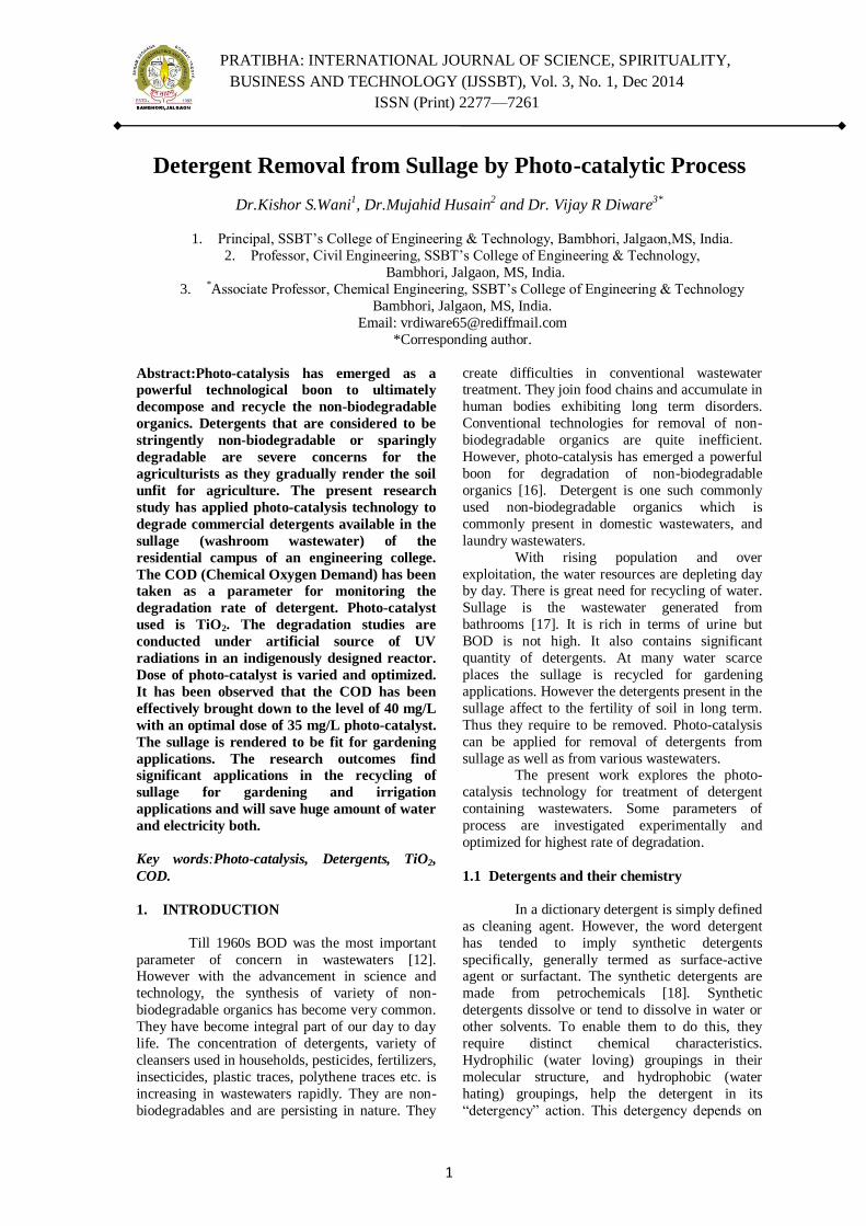
indigenously designed reactor is as shown in the
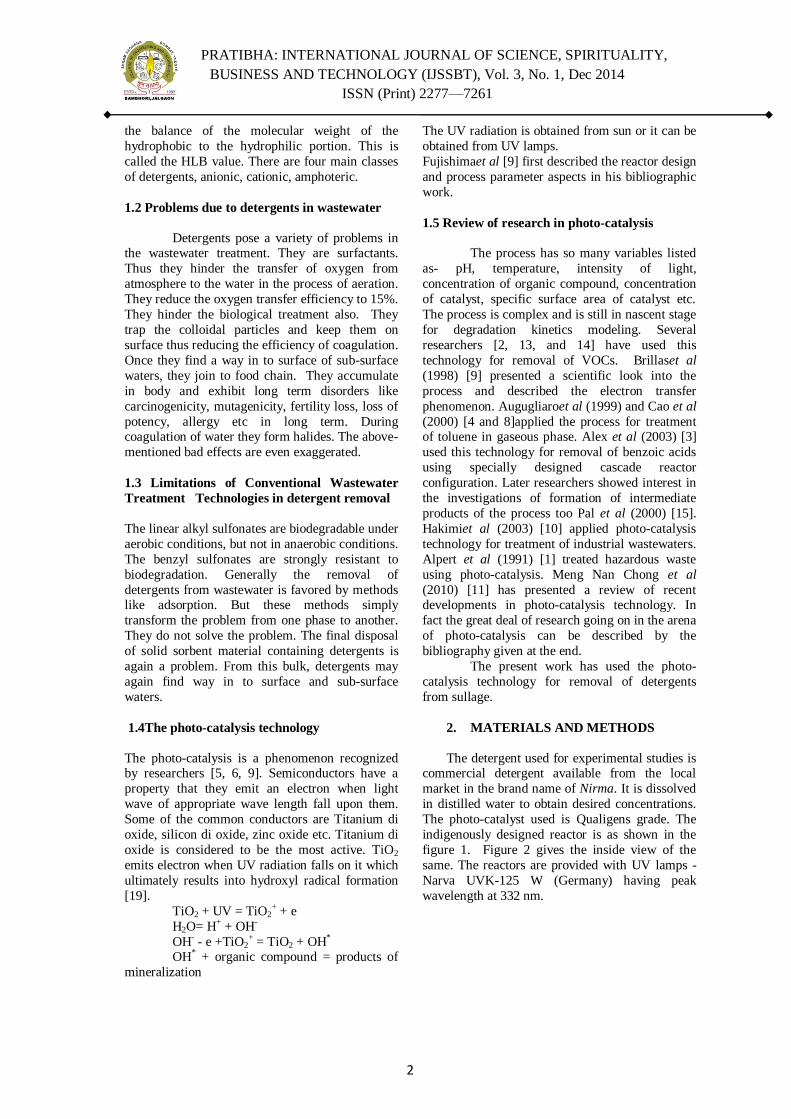
figure 1. Figure 2 gives the inside view of the
same. The reactors are provided with UV lamps -
Narva UVK-125 W (Germany) having peak
wavelength at 332 nm.
PRATIBHA: INTERNATIONAL JOURNAL OF SCIENCE, SPIRITUALITY,
BUSINESS AND TECHNOLOGY (IJSSBT), Vol. 3, No. 1, Dec 2014
ISSN (Print) 2277—7261
3
Fig 2: Inside view of slurry type reactor.
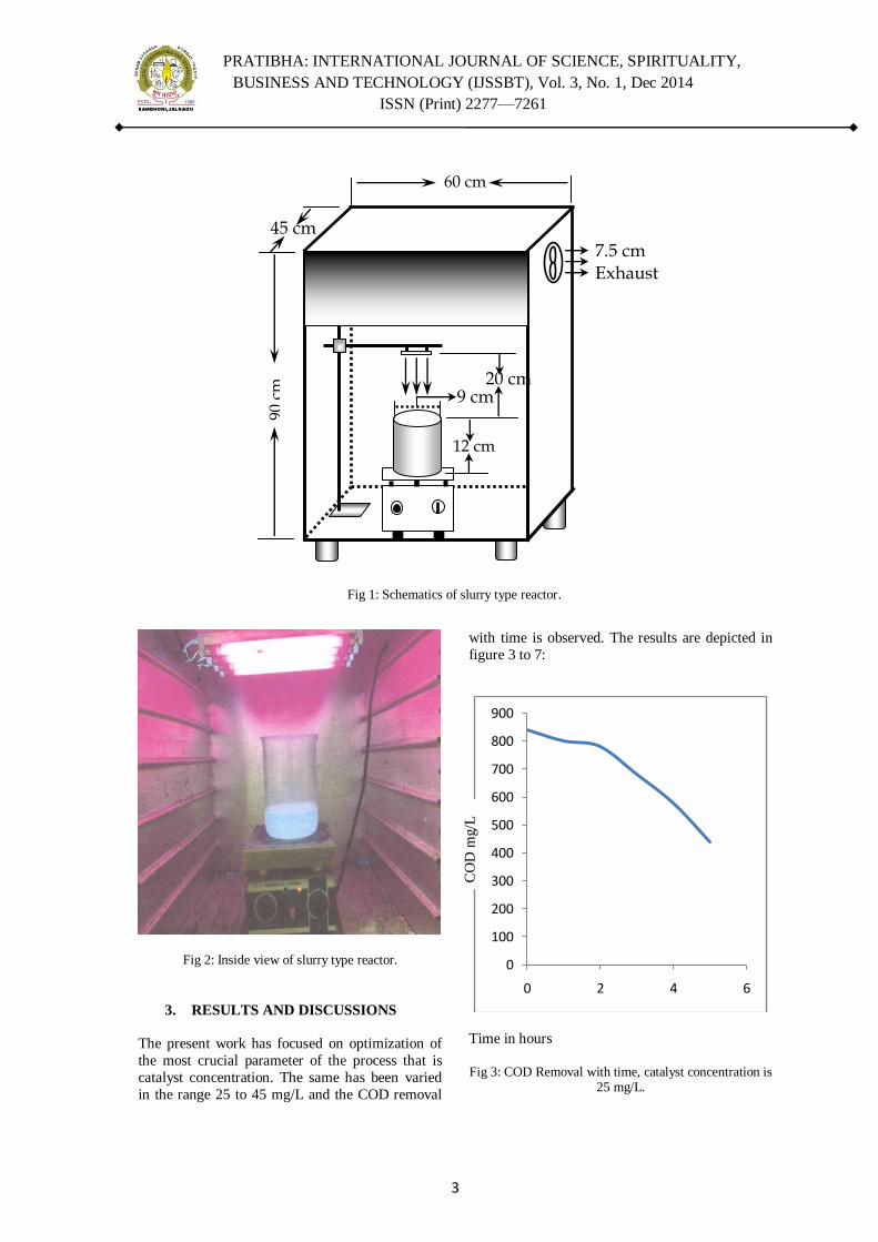
3. RESULTS AND DISCUSSIONS
The present work has focused on optimization of
the most crucial parameter of the process that is
catalyst concentration. The same has been varied
in the range 25 to 45 mg/L and the COD removal
with time is observed. The results are depicted in
figure 3 to 7:
Time in hours
Fig 3: COD Removal with time, catalyst concentration is
25 mg/L.
0
100
200
300
400
500
600
700
800
900
0 2 4 6
CO
D m
g/L
7.5 cm Exhaust Fan I. U
V
R
E
A
C
T
O
R
90 c
m
45 cm
60 cm
9 cm
12 cm
20 cm
Fig 1: Schematics of slurry type reactor.
PRATIBHA: INTERNATIONAL JOURNAL OF SCIENCE, SPIRITUALITY,
BUSINESS AND TECHNOLOGY (IJSSBT), Vol. 3, No. 1, Dec 2014
ISSN (Print) 2277—7261
4
Time in hours
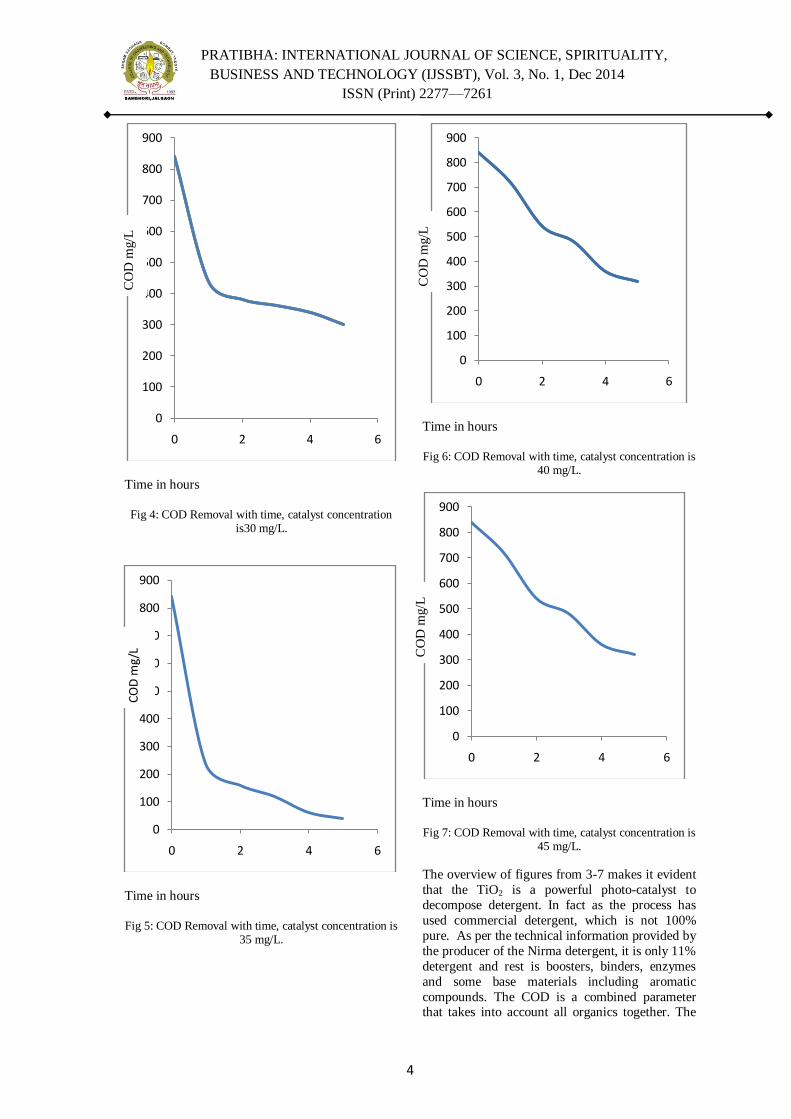
Fig 4: COD Removal with time, catalyst concentration
is30 mg/L.
Time in hours
Fig 5: COD Removal with time, catalyst concentration is
35 mg/L.
Time in hours
Fig 6: COD Removal with time, catalyst concentration is
40 mg/L.
Time in hours
Fig 7: COD Removal with time, catalyst concentration is
45 mg/L.
The overview of figures from 3-7 makes it evident
that the TiO2 is a powerful photo-catalyst to
decompose detergent. In fact as the process has
used commercial detergent, which is not 100%
pure. As per the technical information provided by
the producer of the Nirma detergent, it is only 11%
detergent and rest is boosters, binders, enzymes
and some base materials including aromatic
compounds. The COD is a combined parameter that takes into account all organics together. The
0
100
200
300
400
500
600
700
800
900
0 2 4 6
0
100
200
300
400
500
600
700
800
900
0 2 4 6
0
100
200
300
400
500
600
700
800
900
0 2 4 6
0
100
200
300
400
500
600
700
800
900
0 2 4 6
CO
D m
g/L
C
OD
mg/
L
CO
D m
g/L
C
OD
mg/L

PRATIBHA: INTERNATIONAL JOURNAL OF SCIENCE, SPIRITUALITY,
BUSINESS AND TECHNOLOGY (IJSSBT), Vol. 3, No. 1, Dec 2014
ISSN (Print) 2277—7261
5
figures also indicate that the catalyst concentration
has a profound effect on the degradation rate. 35
mg/L catalyst concentration has come out to be the
optimum as it results into the minimum COD.
The catalyst concentration has complex effect on
degradation of organics. As the degradation
reaction takes place on the surface of the catalyst,
the higher surface area will obviously have high degradation rate. In consequence, it requires higher
concentration of the catalyst. However the reaction
is driven by UV radiation. Hence its penetration in
the liquid slurry is also equally important. The
higher concentration of the catalyst can hinder the
radiation penetration, resulting into lowered
reaction rate. Hence, an optimization is required.
In the present study, the optimal catalyst
concentration comes out to be 35 mg/L. it must be
recognized that the optimum dose is subjected to
other variable combinations like pH, intensity of
light, initial organic concentration etc.
4. CONCLUSIONS
Photo-catalysis is an effective method of removal
of detergents from water. The method can be
effectively applied for sullage which is produced in
large quantity from residential areas and campuses.
It can be easily recycled for irrigation applications.
The laundry wastewaters are rich in terms of
detergents. They can also treated by this method.
The present work has optimized the catalyst concentration for degradation of detergent, the
future researchers may like to optimize other
parameters also for the same.
5. REFERENCES
[1] Alpert Daniel J., Jeremy L. Sprung, James E. Pacheco,
Michael R. Prairie, Hugh E. Reilly, Thomas A. Milne
and Mark R. Nimlos [1991] ―Sandia National
Laboratories‘ work in solar detoxification of
hazardous wastes‖. Solar Energy Materials 24, 594-
607.
[2] AlbericiRosana M. and Wilson F. Jardim [1997]
―Photocatalytic destruction of VOCs in the gas-phase
using titanium dioxide‖. Applied Catalysis B:
Environmental 14, 55-68.
[3] Alex H. C.,Chak K. Chan, John P. Barford and John F.
Porter [2003] ―Solar photocatalytic thin film cascade
reactor for treatment of benzoic acid containing
wastewater‖. Water Research 37, 1125–1135.
[4] Augugliaro Vincenzo, S. Coluccia, V. Loddo and M.
Schiavello [1999] ―Photocatalytic oxidation of
gaseous toluene on anatase TiO2 catalyst: mechanistic
aspects and FT-IR investigation‖. Applied Catalysis
B: Environmental 20, 15-27.
[5] Blake Daniel M. [1996] ―Bibliography of work on the
heterogeneous photocatalytic removal of hazardous
compounds from water and air‖. Update No. 2 To
October 1996, NREL, Golden Co, Technical
Information Service, US Department of Energy,
Springfield.
[6] Blake Denial M., John Webb, Craig Turchi and
Kimberly Magrini [1991] ―Kinetic and mechanistic
over view of TiO2-Photocatalyzed oxidation reactions
in aqueous solution‖. Solar Energy Materials 24, 584-
593.
[7] BrillasEnric, Eva Mur, RoserSauleda, Laura Sanchez,
Jose Peral, Xavier Domenech, Juan Casado [1998]
―Aniline mineralization by AOP‘s: anodic oxidation,
photocatalysis, electro-fenton and photoelectro-fenton
processes‖. Applied Catalysis B: Environmental 16,
31-42.
[8] Cao Lixin, ZiGao, Steven L. Suib, Timothy N. Obee,
Steven O. Hay and James D. Freihaut [2000]
―Photocatalytic oxidation of toluene on nano-scale
TiO2 catalysts: studies of deactivation and
regeneration―. Journal of catalysis 196(2), 253-261.
[9] Fujishime Akira and Rao Tata N. [1998] ―Interfacial
photochemistry: fundamentals and applications‖. Pure
and Applied Chemistry 70 (11), 2177-2187.
[10] HakimiGamil, Lisa H. Studnicki and Muftah Al-
Ghazali [2003] ―Photocatalytic destruction of
potassium hydrogen phthalate using TiO2 and sunlight:
application for the treatment of industrial wastewater‖.
Journal of Photochemistry and Photobiology A:
Chemistry 154, 219–228.
[11] Meng Nan Chong, Bo Jin, Christopher W.K., Chow,
and Chris Saint (2010) Recent developments in photo-
catalytic water treatment, technology: A review,
Water Research, 44, 2997- 3027.
[12] Metcalf and Eddy Inc. (2002) Wastewater treatment,
disposal and reuse 4e, Tata McGraw Hill Publication,
New Delhi.
[13] Okamoto Ken-ichiYasunori Yamamoto, Hiroki
Tanaka, Masashi Tanaka and Akira Itaya et al [1985a]
―Heterogeneous photocatalytic decomposition of
phenol over TiO2 powder‖. Bulletin Chemical Society
Japan 58, 2015-2022.
[14] Okamoto Ken-ichi, Yasunori Yamamoto, Hiroki
Tanaka and Akira Itaya et al [1985b] ―Kinetic of
heterogeneous photocatalytic decomposition of phenol
over anatase TiO2 powder‖. Bulletin Chemical Society
Japan 58, 2023-2028.
[15] Pal Bonmali and Maheshwar Sharon [2000]
―Photodegradation of polyaromatic hydrocarbons over
thin film of TiO2 nanoparticles; a study of
intermediated photoproducts‖. Journal of Molecular
Catalysis A: Chemical 160, 453-460.
[16] Somorjai G. A., N. Serpone and E. Pelizzetti [1989]
―Photocatalysis- Fundamentals and Applications‖.
Hand Book Wiley-Interscience, New York, chapter 9.
[17] Steel E W and Terence J McGhee [1985] Water
supply and sewerage 5e, McGraw Hill Publishing Co.,
New York.
[18] Tyebkhan G (2002), "Skin cleansing in neonates and
infants-basics of cleansers", Indian J Pediatr 69 (9):
767–9.
[19] Turchi Craig S. and David F. Ollis [1990]
―Photocatalytic degradation of organic water
contaminants: mechanisms involving hydroxyl radical
attack‖. Journal of Catalysis 122, 178-192.
PRATIBHA: INTERNATIONAL JOURNAL OF SCIENCE, SPIRITUALITY,
BUSINESS AND TECHNOLOGY (IJSSBT), Vol. 3, No. 1, Dec 2014
ISSN (Print) 2277—7261
6
AUTOMATIC PRODUCT HANDLING, IDENTIFICATION
AND SORTING USINGLabVIEW
Sachin S. Nerkar, Mahesh S. Patil
Instrumentation Department, Government Engineering College, Jalgaon.
ABSTRACT: Till date automation in small and
medium scale industries has not enjoyed the
same rate of growth as in other information
technology sectors, lagging significantly behind
automation in large batch production. The use
of LabVIEW in controlling a robotic arm is a
latest technique which is being implemented in
this project. Through this project our efforts
are to increase the efficiency by building an
automated system which would employ and also
reduces manpower. It involves the use of a
robotic arm which would identify the object
positioning, pick it and then place it in the
desired location. With the use of this system the
process of packaging can be done effectively
without any manpower and also does not
require constant monitoring and guidance. This
paper focuses on designing a robotic arm for
picking and placing an object controlled using
LabVIEW. This is expected to improve the
accuracy and simplicity in control.
INTRODUCTION
Robot is a machine to execute different
task repeatedly with high precision. Thereby many
functions like collecting information and studies about the hazardous sites which is too risky to send
human inside. Robots are used to reduce the
human interference nearly 50 percent. The first
robotic arm to be used in an automobile
Industry was ―UNIMATE‖ in GM motors
USA in 1950s. From then there has been
tremendous improvement in the research and
development in robotics. Now robots are an
integral part of almost all industries. In this paper,
we introduce LabVIEW based control of the robotic arm. The action of picking or placing is
also given through the LabVIEW panel. We have
gained substantial experience when using the
LabVIEW real-time programming environment
coupled with the industrial- quality data
acquisition cards, both made by National
Instruments. The methodology of virtual
instruments (VI) software tools combined with the
graphical programming environment was found to
be very efficient for interactive cycles of design
and testing which are at the core of robotics
prototyping.
MECHANICAL HARDWARE
1. Robotic Arm
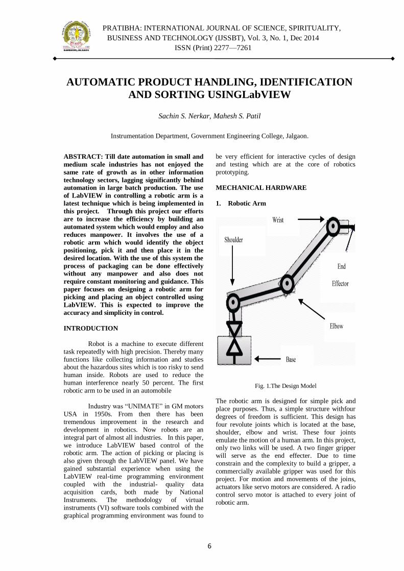
Fig. 1.The Design Model
The robotic arm is designed for simple pick and
place purposes. Thus, a simple structure withfour
degrees of freedom is sufficient. This design has
four revolute joints which is located at the base,
shoulder, elbow and wrist. These four joints
emulate the motion of a human arm. In this project, only two links will be used. A two finger gripper
will serve as the end effecter. Due to time
constrain and the complexity to build a gripper, a
commercially available gripper was used for this
project. For motion and movements of the joins,
actuators like servo motors are considered. A radio
control servo motor is attached to every joint of
robotic arm.

PRATIBHA: INTERNATIONAL JOURNAL OF SCIENCE, SPIRITUALITY,
BUSINESS AND TECHNOLOGY (IJSSBT), Vol. 3, No. 1, Dec 2014
ISSN (Print) 2277—7261
7
2. PC-Based Data Acquisition (DAQ)
Fig. 2 DAQ MX 6009 Card
DAQ is data acquisition. It is device
which contains both ADC and DAC in it. It is
interface between analog output of sensor and the
PC. The data traditinal experiments in it signal
from sensors o are sent to analog or digital domain,
read by experimenter, and recorded by hand. In
automated data acquisition systems the sensors
transmit a voltage or current signal directly to a
computer via data acquisition board. Software such
as LabVIEW controls the acquisition and processing of such data. The benefits of automated
systems are many such as:
1. Improved accuracy of recording
2. Increased frequency with which measurements
can be taken
3. Potential to automate pre and post processing
and built in quality control
The device range can be as follows;
Minimum and maximum voltages the ADC can
digitize. DAQ devices often have different
available ranges. 1. 0 to +10 volts
2. -10 to +10 volts
ROLE OF LabVIEW
A. Introduction to LabVIEW
LabVIEW (Laboratory Virtual Instrument
Engineering Workbench) is a development
environment based on graphical programming. It is
a graphical programming language that uses icons instead of lines of text to create applications. In
contrast to text based programming languages,
where instructions determine program execution,
LabVIEW dataflow programming, where data
determine execution. LabVIEW empowers to build
solutions for scientific and engineering systems.
LabVIEW gives flexibility and performance of a
powerful programming language without the
associated difficulty and complexity.
B. Front Panel
The front panel is the user interface of the VI [10].
We build the front panel with controls and
indicators, which are the interactive input and
output terminals of the VI respectively. Controls are knobs, push buttons, dials, and other input
devices. Indicators are graphs, LEDs and other
displays. Controls simulate instrument input
devices and supply data to the block diagram of the
VI. Indicators simulate instrument output devices
and display data the back panel acquires or
generates.
C. Control Palette
The various sub palettes used are,
Numeric controls sub palette: numeric controls are
included in the front panel for user interface to change the gain values in the design of the PID
controller.
Graph sub-palette: graph indicators are used for
generating the response curves of the system.
D. Function Palette
The function palette is available only on the block
diagram. The functions palette contains the VIs
and functions used to build the block diagram.
Select window >> Show Function Palette or Right-
Click the block diagram workspace to display the Function palette .The Functions Palette can be
placed anywhere on screen. Different hardware
and software components can make the virtual
instrumentation system. There is wide variety of
hardware components can be used to monitor or
control a process or test a device.
E. Tools Palette
The tools palette used in front panel and block
diagram. The Tool palette is available on the front
panel and block diagram. A tool is a special operating mode of
the mouse cursor. While selecting a tool, the cursor
icon changes to the tool icon. Use the tools to
operate and modify front panel and block diagram
objects. Select Window>> show Tools palette to
display the Tools palette and it can be placed
anywhere on the screen.
F. Block Diagram
After building the front panel, add code using
graphical representation of control with front panel
objects. The block diagram contains this graphical source code. Front panel objects appear as
terminals from the block diagram. Every control or
indicator on the front panel has a corresponding
terminal on the block diagram. Additionally, the

PRATIBHA: INTERNATIONAL JOURNAL OF SCIENCE, SPIRITUALITY,
BUSINESS AND TECHNOLOGY (IJSSBT), Vol. 3, No. 1, Dec 2014
ISSN (Print) 2277—7261
8
block diagram contains functions and structures
from build-in LabVIEW VI libraries. Wires
connect each of the nodes on the block diagram,
including control and indicator terminal, function,
and structure.
G. Interfacing
RS232 is interfaced with PIC microcontroller series 16F877A which acts as interface between
mechanical setup (drivers) and LabVIEW.
LabVIEW acts as a controller for the entire process
and interfacing mechanism shown below figure
Fig. 3 Interfacing Mechanism
RESULTS
The Front panel and Block Diagram of LabVIEW
is shown below
A. Front Panel
The fig3.Shows the front panel of the LabVIEW,
where the process can be initiated, controlled,
terminated and indicates the position of Robotic
Arm. The Front Panel also alerts and indicates the
error in circuit connection.
Fig. 4 Front Panel of the Process
B. Block Diagram
The Figure shows the Block diagram of LabVIEW.
The VI shown in the diagram is the overall control
mechanism of automated robotic arm.
Fig 5 VI program of the overall process

PRATIBHA: INTERNATIONAL JOURNAL OF SCIENCE, SPIRITUALITY,
BUSINESS AND TECHNOLOGY (IJSSBT), Vol. 3, No. 1, Dec 2014
ISSN (Print) 2277—7261
9
CONCLUSION AND FUTURE WORK
Acquisition of measurements and modification
of actuations are the usual tasks carried out by
LabVIEW TM and DAQ boards. This
implementation paradigm based on personal
computer and standard operating systems constitutes a new trend in automation. It allows
the user to avoid such aged, specialized or
expensive solutions as analog PID loops,
programmable logic controllers (PLC) or
dedicated hardware based on digital signal
processors (DSP).
REFERENCES
[1] Shyam.R.Nair, ―Design of an Optically
Controlled Robotic Arm for Picking and Placing
an Object‖, International Journal for Scientific
and Research Publications, Vol 2, Issue 4, April
2012.
[2] AmonTunwannarux, and SupanuntTunwannarux
―Design of a 5-Joint Mechanical Arm with User-
Friendly Control Program‖ World Academy of
Science, Engineering and Technology 27 2007
[3] RedwanAlqasemi and Rajiv Dubey ―Control of a
9-DoF Wheelchair-Mounted Robotic Arm
System” 2007 Florida Conference on Recent
Advances in Robotics, FCRAR 2007
[4] JegedeOlawale, AwodeleOludele, AjayiAyodele
and NdongMiko Alejandro “Development of a
Microcontroller Based Robotic Arm”
Proceedings of the 2007 Computer Science and
IT Education Conference.
[5] Brandi House, Jonathan Malkin, Jeff Bilmes“The
VoiceBot: A Voice Controlled Robot Arm‖ CHI
2009, April 4-9, 2009, Boston, Massachusetts,
USA.

PRATIBHA: INTERNATIONAL JOURNAL OF SCIENCE, SPIRITUALITY,
BUSINESS AND TECHNOLOGY (IJSSBT), Vol. 3, No. 1, Dec 2014
ISSN (Print) 2277—7261
10
The Study of Internet Banking Usage: A Case study of SBI
Dana Bazaar Branch, Jalgaon.
Mukesh B. Ahirrao1, Pankajkumar A. Anawade
2, Mangesh Mali
3
1 Asst. Prof, M.B.A Dept., S.S.B.T‘s College of Engineering & Technology, Bambhori, Jalgaon, MS
(Corresponding Author) 2 Asst. Prof, M.B.A Dept., S.S.B.T‘s College of Engineering & Technology, Bambhori, Jalgaon, MS
3 Student, M.B.A Dept., SSBT‘s College of Engineering & Technology, Bambhori, Jalgaon, MS, India
Emails: [email protected]
Abstract: SBI is pioneer in internet banking.
But it does not mean to say that implement of
new technology is always advantages because
actual use of technology is also important.
Objective of this study is to analyze the
awareness and usage of internet banking among
the account holders of SBI Dana bazaar branch
Jalgaon. The objective of selecting this case
study is felt due to the fact that most of the
account holders of SBI Dana bazaar branch are
business and trading firms. Banking
transactions are vast among these account
holders. And they can be benefited much from
the internet banking. The study is based on the
primary data collected through questionnaire
from 75 accounts holder of SBI, Dana Bazaar
Branch. The study reveals good awareness of
internet banking among respondents but
limited to content and information sharing only.
They are still not habitual to use internet
banking for transaction purpose.
Keywords: Internet Banking & its Usage, SBI,
Digital Baking, Electronic Banking.
I. INTRODUCTION: INTERNET
BANKING
Internet Banking System is a system that
has been developed in order to help clients to do
day-to-day transactions electronically from any
place. Internet banking systems means that clients
can now do banking at the leisure of their homes.
It is also known as online banking, the system allows both transactional and non-
transactional features. Online banking or internet
banking allows customers to conduct financial
transactions on a secure website operated by the
retail or virtual bank. (Kaushik, 2012)
Products and Services offered by SBI:
1. E-Ticketing
2. SBI E-Tax
3. RTGS/NEFT
4. E-Payment
5. Fund Transfer
6. Third Party Transfer
7. Demand Draft
8. Cheque Book Request
9. Account Opening Request
10. Account Statement
11. Transaction Enquiry
12. Demat Account Statement
1. E-Ticketing: E-Ticketing provides service to book railway, air
and bus tickets online through Online SBI.
Railway ticket can be booked through irctc.co.in.
Railway tickets are available in to forms.
I-ticket (where the delivery of tickets will be
made at your address) or
E-tickets (e-ticket is generated & can be
printed at home.)
Air flight tickets and selected bus transport ticket
of metro cities are also available through E-Ticket
Services
2. SBI E-Tax:
This facility enables to pay TDS, Income tax,
Indirect tax, Corporation tax, Wealth tax, Estate
Duty and Fringe Benefits tax online through SBI
E-Tax. The online payment feature facilitates
anytime, anywhere payment and an instant E-
Receipt is generated once the transaction is
complete. The Indirect Tax payment facility is
available to Registered Central Excise/Service Tax
Assesses who possesses the 15 digit PAN based Assesses Code.
3. E-Payment:
A simple and convenient service for viewing and
paying bills online. Using the bill payment
anybody can view and Pay various bills online,
directly from your SBI account. It can pay
telephone, electricity, insurance, credit cards and
other bills from the comfort of your house or
office, 24 hours a day, 365 days a year.

PRATIBHA: INTERNATIONAL JOURNAL OF SCIENCE, SPIRITUALITY,
BUSINESS AND TECHNOLOGY (IJSSBT), Vol. 3, No. 1, Dec 2014
ISSN (Print) 2277—7261
11
It can also set up Auto Pay instructions with an
upper limit to ensure that your bills are paid
automatically whenever they are due.
4. RTGS/NEFT:
It can transfer money from State Bank account to
accounts in other banks using the RTGS/NEFT
service. The RTGS system facilitates transfer of funds from accounts in one bank to another on a
"real time" and on "gross settlement" basis. This
system is the fastest possible interbank money
transfer facility available through secure banking
channels in India. It can transfer an amount of Rs.1
lacs and above using RTGS system. National
Electronic Funds Transfer (NEFT) facilitates
transfer of funds to the credit account with the
other participating bank.
5. Fund Transfer:
The Funds Transfer facility enables to transfer funds within accounts in the same branch or other
branches. It can transfer aggregating Rs.1 lacs per
day to own accounts in the same branch and other
branches. To make a funds transfer, it should be an
active Internet Banking user with transaction
rights. Funds transfer to PPF account is restricted
to the same branch.
6. Third Party Transfer:
It can transfer funds to trusted third party‘s account
by adding them as third party accounts. The beneficiary account should be of any SBI branch.
Transfer is instant. it can do any number of
Transactions in a day for amount aggregating
Rs.1lakh.
7. Demand Draft:
The Internet Banking application provides to
register demand drafts requests online. You can get
a demand draft from any of your Accounts
(Savings Bank, Current Account, Cash Credit or
Overdraft). Limit can be set to issue demand drafts from your accounts or use the bank specified limit
for demand drafts. A printed advice can also be
obtained from the site for record purpose.
8. Cheque Book Request:
A request can be posted through internet banking
account for a cheque book. Cheque book can be
requested for any Savings, Current, Cash Credit,
and Over Draft accounts. It enables to opt for
cheque book with 25, 50 or 100 cheque leaves.
Cheque book can be delivered to registered address
or any other address provided in request.
9. Account Opening Request:
OnlineSBI enables it to open a new account online.
You can apply for a new account only in branches
where you already have accounts. You should have
an INB-enabled account with transaction right in
the branch. Funds in an existing account are used
to open the new account. You can open Savings,
Current, Term Deposit and Recurring Deposit
accounts etc.
10. Account Statement: The Internet Banking application can generate an
online, downloadable account statement for any
accounts for any date range and for any account
mapped to username. The statement includes the
transaction details, opening, closing and
accumulated balance in the account. The account
statement can be viewed online, printed or
downloaded as an Excel or PDF file.
11. Transaction Enquiry:
OnlineSBI provides features to enquire status of
online transactions. It can view and verify transaction details and the current status of
transactions.
12. Demat Account Statement :
OnlineSBI enables it to view Demat account
statement and maintain such accounts. The bank
acts as your depository participant. In the third
party site, you can mark a lien on your Demat
accounts and use the funds to trade on stock using
funds in your SBI savings account.
It can provide Demat account details and generate the statement of holding, statement of transactions
and statement of billing. (Kaushik, 2012)
II. OBJECTIVES:
To analyze the awareness & usage of internet
banking by SBI customers.
To identify the strength and weaknesses of it
and reasons of that.
To suggest the appropriate measures to
increase the use of internet banking by
customers.
III. RESEARCH METHODOLOGY
Type of Research: it is a survey research
method collecting actual facts and figures.It is
descriptive in nature using both primary and
secondary data. Secondary data is used to
conceptualize the objective, nature and scope of
the survey. And primary data is used to collect
actual facts regarding proposed problems in
objectives.
Types of Data:
Primary data: primary data were collected
through structured questionnaire methods.
Primary data includes actual facts about

PRATIBHA: INTERNATIONAL JOURNAL OF SCIENCE, SPIRITUALITY,
BUSINESS AND TECHNOLOGY (IJSSBT), Vol. 3, No. 1, Dec 2014
ISSN (Print) 2277—7261
12
awareness and usage of computer, internet and
internet banking. Some formal discussions are
held with branch manager to know additional
information about the branch, its customers and
their professions.
Secondary data: Secondary data were
collected through various sources such as official‘s reports & websites etc. most of the
secondary data is collected through internet.
Sample Size: There are 183 accounts holders
of SBI Dana Bazaar Branch. Out of which 112
are current account of trading firms. 96 of
which are found active and 75 accounts are
taken as sample for the study.
IV. Data Analysis and Interpretation:
1. Use of Computer for Fun, Work and
Personal Purpose per Week:
Sources: Primary Data.
Fig. 1: Use of Computer Hours
Interpretation:
Figure 1 reflects Computer hours required for
office work is high (> 20 Hrs) as compared to fun
and personal purpose (1-10 Hrs). But more clients are found using computer for fun and personal
purpose against work. Use of computer for work is
very limited in spite of its advantages.
2. Frequency of Bank Visit per Week:
Sources: Primary Data.
Fig. 2
Interpretation:
Figure 2 reflects 72 % of clients visit bank for
transaction purpose. The frequency of these clients
is between 2 to 8 visits per week. This frequency is positive from the internet usage point of view.
3. Use of Internet Banking Facility:
Source: Primary Data
Fig. 3: Use of Internet Banking Facility.
Interpretation:
Figure 3 reflects use of internet banking for
various purposes. Most of the clients of SBI Dana
Bazaar Branch are using internet banking facility
for Seeking product and rate information,
Calculate loan payment information, Download
loan application, Download personal bank
transaction activity, Check balance on-line. That is
majority of clients are using internet banking
facility for searching information on product or services offered by bank. Very few clients are
using internet banking for On-line bill payment.
0
10
20
30
40
50
60
70
80
90
< 1 hrs
1 To 5
hrs
5 To 10 hrs
10 to 20 hrs
> 20 hrs
14
2917
0 2
2
23
11
3
23
20
34
3
5
0
Use for Personal Purpose
Use for Work
Use for Fun
1820
24
0 00
5
10
15
20
25
30
< 1 1 To 3 Times
3 To 8 times
8 To 12
times
> 12 times
Frequency of Bank Visit
0102030

PRATIBHA: INTERNATIONAL JOURNAL OF SCIENCE, SPIRITUALITY,
BUSINESS AND TECHNOLOGY (IJSSBT), Vol. 3, No. 1, Dec 2014
ISSN (Print) 2277—7261
13
4. The reasons behind limited use of internet
banking for online transaction purpose:
Interpretation:
Reasons for limited use of internet banking
transaction reported as lack of awareness, concern
of online fraud and internet security, don‘t know how to use it etc.
V. Findings:
Awareness and use of computer as well as
internet:
Majority of client‘s use of computer for
personal and official purpose is good. They are
using www web 2 services as well. They have
performed online transaction. That suggests their
good awareness, use of computer and internet.
Analysis of need for internet banking:
The frequency of visit to bank & ATM
for different transaction purpose is also
considerable. Inter firm transactions are also
considerable among them. Exp. Third party
transfer, bill payments etc. this suggest there is
good scope to use internet banking for day to day
transaction purpose.
Strength & Weaknesses:
Most of the clients of SBI Dana Bazaar Branch are using internet banking facility for
Seeking product and rate information, Calculate
loan payment information, Download loan
application, Download personal bank transaction
activity, Check balance on-line. That is majority of
clients are using internet banking facility for
searching information on product or services
offered by bank.
But Very few clients are using internet
banking for On-line transaction purpose. The
reasons are lack of awareness, concern of online fraud and internet security; don‘t know how to use
it.
VI. Suggestions:
Bank can provide user‘s manuals as well as
Training to the customers so that they can be
inclined to use the internet banking for
transaction purpose.
Training can be provided on following
aspects:-
o Online Fund Deposit
o Online Fund transfer, RTGS, NEFT o Online Third party transfer
o Online Tax filling
o Online Bill Payment etc.
Such a training programme can be frequently
introduced for new customers.
VII. Conclusions:
Internet banking is gaining popularity and
it is very essential for new age customer. Use of
internet banking is very beneficial to customers as
it saves lots of harassment and cost incurred on the coordination for banking transaction.
From the above analysis, I conclude that,
awareness of computers, internet and internet
banking among SBI account holder is high as well
as use of computer and internet for personal and
official purpose is also good. Similarly, Use of
internet banking is high for searching online
information but, in spite of its advantages, use of
internet banking for online transaction purpose is
very limited.
VIII. References:
[1] E-Pay. (n.d.). Frequently Asked Questions. Retrieved
March 15, 2014, from State Bank of India:
http://www.sbi.co.in/
[2] Internet Banking. (n.d.). Frequently Asked Questions.
Retrieved March 15, 2014, from State Bank of India:
www.onlinesbi.com
[3] Kaushik, A. K. (2012). E-BANKING SYSTEM IN SBI.
ZENITH, International Journal of Multidisciplinary
Research, Vol.2 (Issue 7), 01 - 22.
[4] RTGS/ NEFT. (n.d.). Frequently Asked Questions.
Retrieved March 15, 2014, from State Bank of India:
http://www.sbi.co.in/
[5] SBI Internet Banking. (n.d.). Home » SBI Bank » Internet
Banking. Retrieved March 15, 2014, from Online Banks
Guide: http://www.onlinebanksguide.com/
[6] State Bank of India. (2013). Customer Manual for Deposit
Accounts. New York Branch, NY 10022, U.S.A., Deposit
Section. State Bank of India.

PRATIBHA: INTERNATIONAL JOURNAL OF SCIENCE, SPIRITUALITY,
BUSINESS AND TECHNOLOGY (IJSSBT), Vol. 3, No. 1, Dec 2014
ISSN (Print) 2277—7261
14
Green HR Practices: An Empirical Study of Cargill, Jalgaon
Dr. VishalS.Rana 1, Ms. Sonam N.Jain
2
1Asst Prof & Head, M.B.A Dept, S.S.B.T‘s College of Engineering & Technology, Bambhori, Jalgaon, MS
(Corresponding Author) 2 Student, Department of Business Administration, SSBT‘s College of Engineering & Technology,
Bambhori, Jalgaon, MS, India.
Emails: [email protected], [email protected]
ABSTRACT: There is a growing need for the
integration of environmental management into
Human Resource Management (HRM) – Green
HRM – research practice. A review of the
literature shows that a broad process frame of
reference for Green HRM has yet to emerge. A
concise categorization is needed in this field to
help academics, researchers and practitioners,
with enough studies in existence to guide such
modeling. This article takes a new and
integrated view of the literature in Green HRM,
using it to classify the literature on the basis of
entry-to-exit processes in HRM (from
recruitment to exit), revealing the role that HR
processes play in translating Green HR policy
into practice. The contribution of this article
lies in drawing together the extant literature in
this area, mapping the terrain in this field, and
in proposing a new process model and research
agenda in Green HRM.The Greening of HR
Survey examines the types of environmentally
friendly "green" initiatives that companies are
utilizing involving their workforce and human
resource practices. The results confirm that
companies are incorporating and working
toward integrating a number of green practices.
The world is a smaller place thanks to the
Internet, global trading and new
communication and technology. More
companies are expanding overseas and now
manage a global workforce that has unique
benefits, rules/laws and different languages and
currencies.
I. INTRODUCTION TO GREEN HR
―Green HR‖ is an employment model designed to
assist industry professionals in retaining, recalling,
preserving and developing talent needed to ensure
future business initiatives and strategies are met.
Efficiency afforded by the ―Green HR‖ model can
lower operational costs and enables industry
professionals to better utilize their investment in
knowledge capital, Green HR is one which
involves two essential elements: environmentally
friendly HR practices and the preservation of
knowledge capital. Green HR involves reducing
your carbon footprint via less printing of paper,
video conferencing and interviews, etc. Companies
are quick to layoff when times are tough before
realizing the future implications of losing that
knowledge capital. Green HR initiatives help
companies find alternative ways to cut cost without
losing their top talent; furloughs, part time work,
etc.
II. OBJECTIVES OF THE STUDY
To study the effectiveness of Green HR
mechanism at Cargill.
To determine current green sustainability of
Cargill.
To determine measures of green success.
To understand that how Green HR policies
and practices can improve the environmental
performance of organizations.
III. RESEARCH METHODOLOGY
The type of research used in this project is
descriptive in nature. Primary data was collected
using the questionnaire. A survey was done with
the researcher meeting the respondents in their
respective places. The respondent‘s reference to
each question was carefully noted in the carefully
observed and registered Questionnaire. Analysis
techniques are used to obtain finding and arrange
information in a logical sequence from the raw
data collected. After the tabulation of data the tools provide a scientific and mathematical solution to a
complex problem.
IV. IMPORTANCE OF THE STUDY
We are entering a green economy-one in which
consumer and employee expectations and future
environmental change will require business to
address ―green‖ issues. Environmental conscious
organizations will become increasingly prominent
as we re-enter into a period of growth. Green HR is
PRATIBHA: INTERNATIONAL JOURNAL OF SCIENCE, SPIRITUALITY,
BUSINESS AND TECHNOLOGY (IJSSBT), Vol. 3, No. 1, Dec 2014
ISSN (Print) 2277—7261
15
a not just a strategy used primarily for reducing the
carbon footprint of each employee and talent
retention. Green HR is one which involves two
essential elements: preservation of knowledge
capital and environmentally friendly HR practices.
Green HR involves reducing your carbon footprint
via less printing of paper, video conferencing and
interviews, etc.Companies are quick to layoff when times are tough before realizing the future
implications of losing that knowledge capital.
Green HR initiatives help companies find
alternative ways to cut cost without losing their top
talent; furlough, part time work etc. ―Green HR‖ is
an employment model designed to assist industry
professionals in retaining, recalling, preserving and
developing talent needed to ensure future business
initiatives and strategies are met. HR professionals
in organization can develop a powerful social
conscience and green sense of responsibility
internal and external customers, stakeholders, partners etc. Recent times, consumers demand
ethics and environmental credentials as a top
priority. Society and business see their agenda
align.
V. PUTTING HUMAN CAPITAL
MANAGEMENT PROCESSES ONLINE
ALSO HELPS TO:
Significantly reduce wasted time and effort in collecting paper forms and building reports.
Push out information right now, rather than
waiting for paper newsletters and forms to be
printed and collected.
Provide easy to use multimedia content
including video, PowerPoint, audio, text,
pictures.
Reduces carbon footprint by reducing paper
usage.
Reduces waste by preventing hard copy from
being thrown in the bin.
Easily gather employee feedback.
Save lot of money on printing costs
Get managers talking more to employees
by streamlining existing processes.
VI. Green Transformation Process of
Cargill
Many organizations are still considering the
feasibility of going green in their business while
others are exploring the desirability to adapt a
green business strategy. However, in order for HR
to consider becoming green and incorporating
green practices in their strategies and people
development plans, it is critical that organizations
adopt a strategic decision to incorporate a green
approach to their desired business results. The most important way to do this is to make changes
to both the internal and external value chain that
defines the business in its industry together with
the competitors and the supply chain that directly
impacts the final business results. The framework
indicates an organization‘s developmental decision
to make the move to green performance within the
context of corporate sustainability.
VII. SURVEY AT CARGILL:
The survey noted that 60% of organizations are
measuring their cost savings – this is up from 39%
last year. Among the organizations that have a
formal green program, the most common practices
are:
Recycling and paper reduction (97%)
Web and/or teleconferencing (95%)
Healthy living and wellness (85%)
Internal green communication programs
(81%).
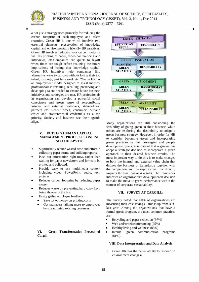
VIII. Data Interpretation and Data Analysis
1. Green HR has the better ability to respond to
environment changes?
PRATIBHA: INTERNATIONAL JOURNAL OF SCIENCE, SPIRITUALITY,
BUSINESS AND TECHNOLOGY (IJSSBT), Vol. 3, No. 1, Dec 2014
ISSN (Print) 2277—7261
16
A) Yes B) No C) None
Inference -from the above pie chart it is found that
in view of 75% respondents green HR has the
better ability to respond to environmental changes
whereas only 15% respondents opined that green
HR does not respond to environmental changes
and 10% respondents are unaware about the green
HR ability.
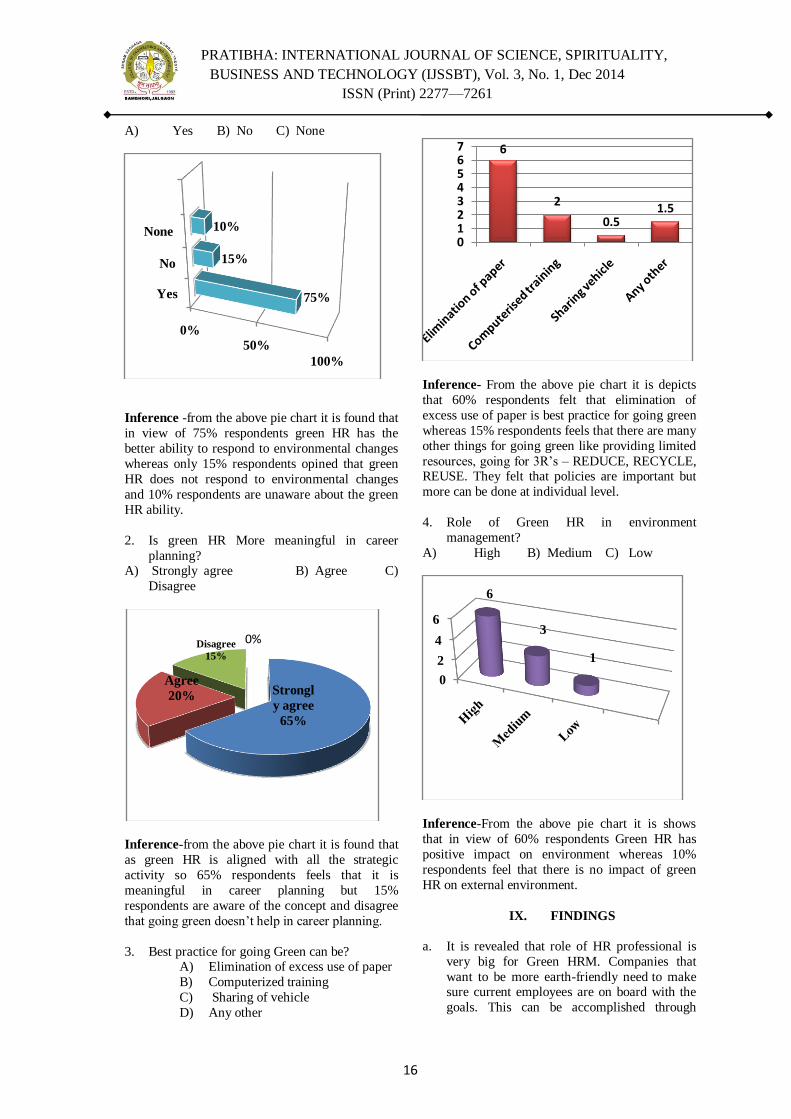
2. Is green HR More meaningful in career
planning? A) Strongly agree B) Agree C)
Disagree
Inference-from the above pie chart it is found that
as green HR is aligned with all the strategic
activity so 65% respondents feels that it is
meaningful in career planning but 15%
respondents are aware of the concept and disagree
that going green doesn‘t help in career planning.
3. Best practice for going Green can be? A) Elimination of excess use of paper
B) Computerized training
C) Sharing of vehicle
D) Any other
Inference- From the above pie chart it is depicts
that 60% respondents felt that elimination of
excess use of paper is best practice for going green
whereas 15% respondents feels that there are many
other things for going green like providing limited
resources, going for 3R‘s – REDUCE, RECYCLE, REUSE. They felt that policies are important but
more can be done at individual level.
4. Role of Green HR in environment
management?
A) High B) Medium C) Low
Inference-From the above pie chart it is shows
that in view of 60% respondents Green HR has
positive impact on environment whereas 10%
respondents feel that there is no impact of green
HR on external environment.
IX. FINDINGS
a. It is revealed that role of HR professional is
very big for Green HRM. Companies that
want to be more earth-friendly need to make sure current employees are on board with the
goals. This can be accomplished through
Yes
No
None
0%
50%
100%
75%
15%
10%
Strongl
y agree
65%
Agree
20%
Disagree
15%
0%
6
2
0.51.5
01234567
0
2
4
6
6
3
1

PRATIBHA: INTERNATIONAL JOURNAL OF SCIENCE, SPIRITUALITY,
BUSINESS AND TECHNOLOGY (IJSSBT), Vol. 3, No. 1, Dec 2014
ISSN (Print) 2277—7261
17
communication and training by the HR
professionals.
b. Discloser of study shows that Impact of Green
awareness is fruitful. There are numbers of
program which offers monthly electronic
communications, including newsletters and
interactive games, as well as working with
companies to appoint green coordinators in local offences to help develop plans and serve
as points of contact for green practices.
c. It is founded that changing attitudes and
behaviours related to environmental issues in
the workplace. Flexibility is often the driver of
change, and it's at the heart of the sustainable
management initiative.
d. It is concluded that it retires burdensome
paper-based processes and improve the
process efficiency.
e. It shows that it also reduces turnaround times
and as well as costs/paper consumption. f. Study shows that it help in additional tools for
automated and business processes.
g. It also revealed that it is important to improve
the Green Hr policies at Employee level for
the better result.
h. It is found that people thinks it‘s very
necessary to go Green but again they don‘t
know how to take the first step so the proper
training and communication should be done.
i. It may also reveal data to add an HRM
element to the knowledge base and Green Management in general for academics.
X. CONCLUSION
It is concluded that Green ideas and concepts are
beginning to gather pace within the HR space,
often complementing existing sustainability-based
initiatives. Increasingly they are delivering
tangible benefits to the business, rather than simply
adding a gloss to brand and reputation. During the
research, researcher has observed the new processes, policies and tools are actually helping to
ensure compliance and improve process too. And
with legislation now in place to effectively
formalize the need for a new corporate approach to
the environment, now's the time for HR to embrace
the green agenda. In future research into Green
HRM may provide interesting results for all
stakeholders in HRM. It is concluded that specific
focus on waste management and recycling; for
employees, they may help them lobby employers
to adopt Green HRM policies and practices that
help safeguard and enhance workers health and well-being.
XI. REFERENCES
[1] Essential of HRM and Industrial Relations by P.Subha Rao
– Himalaya Publications.
[2] Human Resource Management by Ashwathapa – Tata
McGraw Hill.
[3] Comprehensive Human Resource Management By P.L.Rao
- Excel Books
[4] Human Resource Management By Dr. C.B. Gupta – Sultan
Chand & Sons.
[5] Performance Management by Herman Aguinis.- Pearson.
[6] Human Behaviour at Work –Keith Devis-Tata McGraw
Hill.
[7] Human Relations and OrganisationalBehaviour (5/e) -
Dwivedi – Macmillan Publications.
[8] The Citigroup-Environmental Defense Partnership to
Improve Office Paper Management
[9] ―Recycling Facts and Figures,‖ Wisconsin Department of
Natural Resources.
PRATIBHA: INTERNATIONAL JOURNAL OF SCIENCE, SPIRITUALITY,
BUSINESS AND TECHNOLOGY (IJSSBT), Vol. 3, No. 1, Dec 2014
ISSN (Print) 2277—7261
18
ANALYSIS OF SPRING BACK DEFECT IN RIGHT
ANGLE BENDING PROCESS IN SHEET METAL
FORMING
P.S.NANDANWAR1, P.S.BAJAJ
2, P.D. PATIL
3
1Asistant Professor, Department of Mechanical Engineering,
Faculty of S.S.B.T. C.O.E.T.Bambhori, Jalgaon. 2 Associate Professor, Department of Mechanical Engineering,
Faculty of S.S.G.B. C.O.E.T. Bhusawal. 3Asistant Professor, Department of Mechanical Engineering,
Faculty of S.S.B.T. C.O.E.T. Bambhori, Jalgaon.
ABSTRACT: In the project work, the
deformation mechanics of the spring back
phenomenon in the Right Angle Bending of
sheet-metal was examined and a new method
that could efficiently reduce spring back in the
Right Angle Bending of sheet metal was
proposed. Both the finite element analysis and
experiments were performed to analyze the
deformation mechanics and the effects of
process parameters on the formation of spring
back. The axial stress distribution in the bent
sheet obtained by the finite element simulations
was classified into three zones: the bending zone
under the punch corner (zone I), unbending
zone next to the bending zone (zone II), and the
stress-free zone (zone III). It is found that the
stress distribution in zone I is quite uniform and
hence has little influence on the spring back.
While the stress distribution in zone II results in
a positive spring back, whereas the stress
distribution in zone III produces a negative
spring back. The total spring back therefore
depends on the combined effect of those
produced by zone II and zone III. A reverse
bend approach that can efficiently reduce
spring back was also proposed to reduce the
spring back in the Right Angle Bending process.
The finite element analysis performed in the
present study was validated by experiments as
well. Although the reverse bend approach can
reduce spring back efficiently, it may cause
uneven surface at the die corner area. Hence,
the use of reverse bend approach must be
cautious if high surface quality is required. The
proposed reverse bend approach provides the
die design engineer with a novel idea to reduce
the spring back occurred in the Right Angle
Bending of sheet metals. In addition to the
reverse bend approach, the analysis of
deformation mechanics of spring back
performed in the present study also provides
researchers with a better understanding of the
formation of spring back.
INTRODUCTION
Spring back is a main defect occurred in
the sheet-metal forming processes and has been
thoroughly studied by researchers. Among them,
quite a few efforts have been made to obtain a
deep understanding of the spring back
phenomenon. The beam theory has been applied to
formulate the curvature before and after loading by
some researchers [1-3]. Hill [4] also presented a
general theory for the elastic-plastic pure bending
under the plane strain condition. The spring back
occurring in the bending of high strength steels was discussed by Davies [5], and Chu [6]. Nader
[7] examined the effects of process parameters on
the spring back in the V-bending process by
developing theoretical models. In addition to
various theories on prediction of spring back,
efforts were also made to reduce the spring back.
Liu [8] demonstrated an efficient method that
dramatically reduced the spring back using the
double-bend technique. A bending restriking
process was proposed by Nagai [9] to reduce
spring back. Wang [10] showed by conducting experiments that the spring back could be reduced
by the over-bend approach. Chan and Wang [11]
have proposed a strain-hardening plane-stress
bending model to predict the deformation behavior
and spring back of narrow strips. A computer aided
design method for straight flanging using finite
element method was presented by Livatyali and
Altan [12]; they also investigated flanging with
coining as a method to eliminate spring back and
to improve part quality. The finite element
simulation and experimental approach were also
employed by researchers [13-15] to study the spring back and side-wall curl in the sheet metal
forming.

PRATIBHA: INTERNATIONAL JOURNAL OF SCIENCE, SPIRITUALITY,
BUSINESS AND TECHNOLOGY (IJSSBT), Vol. 3, No. 1, Dec 2014
ISSN (Print) 2277—7261
19
In the present study, the Right Angle
Bending process of aluminum alloy AA5052-H34,
as shown in Fig. 1, was studied. The effects of the
process parameters on the spring back occurring in
the Right Angle Bending process were first
examined by both the finite element analysis and
experiments. In addition, the deformation
mechanics of the spring back phenomenon was investigated in detail by the finite element analysis.
A reverse bend approach was then proposed to
reduce the spring back in the Right Angle Bending
process. The proposed approach was demonstrated
to be very efficient by the finite element analysis
and was validated by experiments conducted in the
present study. Performed using aluminum alloy
AA5052-H34 sheet as specimen. Since spring back
is mainly due to the elastic recovery of the stress
distribution along the axial direction, the stress
distributions in the bent sheet obtained from the
finite element simulations were transformed into the axial direction accordingly, and the stress
distribution mentioned hereinafter is associated
with axial direction. Figure 3 shows the stress
distribution in the bent sheet along the axial
direction at the end of bending process before the
punch is removed. Based on the stress distribution
patterns, the bent sheet is classified into three
zones: flat zone under the blank holder, bending
zone at the die corner and unbending zone at side
wall, which are marked by I, II, and III,
respectively, in Fig. 3, and the stress distributions in zone I and zone III are displayed in Fig. 3 as
well. While Fig. 4 displays the stress distribution
in zone II. Since the stress distribution in the flat
zone is nearly uniform compression, it is obvious
that the spring back is independent of the flat zone,
i.e., zones I, and is mainly attributed to the stress
distributions in zone II and zone III.
Fig. 1. A Sketch of Right Angle-Bending
FINITE ELEMENT MODEL
In the present study, the sheet-metal was
assumed to be very wide and the Right Angle
Bending could be simplified to a 2-D plane-strain
problem. The tooling used in the bending process
was modeled as rigid bodies. As for the sheet-
metal, the 4-node plane-stress element was adopted
to construct the mesh. Since the number of
elements in the thickness direction has significant
effect on the accuracy of the simulation, the
convergence tests were performed to determine a
suitable number of elements to be used in the thickness direction. In the present study, 6 layers
of elements in the thickness direction were used in
most of the simulations. After the sheet-metal
being bent into an L-shape, the punch and blank
holder were removed and the spring back was
measured by comparing the difference of the bent
angle before and after the tooling was removed, as
shown in Fig. 2. In each simulation, the Coulomb
friction coefficient was used to describe the
interface friction condition between the tooling and
sheet-blank. The finite element code ABAQUS
was adopted to conduct all the simulations and the material properties of AA5052-H34 obtained from
the tension tests conducted in the present study
were used for the finite element simulations.
Fig. 2 The shapes before and after tooling removal
DEFORMATION MECHANICS IN RIGHT
ANGLE –BENDING
In order to examine the deformation mechanics along the whole sheet after bending, the
finite element simulations were
Fig. 3. Stress distribution in the bent sheet before tooling
removal
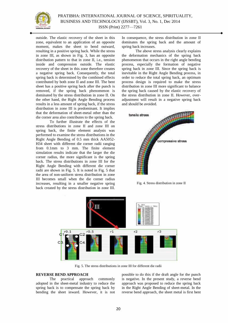
The stress distribution in zone II, as
shown in Fig. 4, follows the bending theory that
the sheet is compressed inside and stretched
PRATIBHA: INTERNATIONAL JOURNAL OF SCIENCE, SPIRITUALITY,
BUSINESS AND TECHNOLOGY (IJSSBT), Vol. 3, No. 1, Dec 2014
ISSN (Print) 2277—7261
20
outside. The elastic recovery of the sheet in this
zone, equivalent to an application of an opposite
moment, makes the sheet to bend outward,
resulting in a positive spring back. While the stress
in zone III, as shown in Fig. 3, has an opposite
distribution pattern to that in zone II, i.e., tension
inside and compression outside. The elastic
recovery of the sheet in this zone therefore creates a negative spring back. Consequently, the total
spring back is determined by the combined effects
contributed by both zone II and zone III. The bent
sheet has a positive spring back after the punch is
removed, if the spring back phenomenon is
dominated by the stress distribution in zone II. On
the other hand, the Right Angle Bending process
results in a less amount of spring back, if the stress
distribution in zone III is predominant. It implies
that the deformation of sheet-metal other than the
die corner area also contributes to the spring back.
To further illustrate the effects of the stress distributions in zone II and zone III on
spring back, the finite element analysis was
performed to examine the stress distributions in the
Right Angle Bending of 0.5 mm thick AA5052-
H34 sheet with different die corner radii ranging
from 0.1mm to 3 mm. The finite element
simulation results indicate that the larger the die
corner radius, the more significant is the spring
back. The stress distributions in zone III for the
Right Angle Bending with different die corner
radii are shown in Fig. 5. It is noted in Fig. 5 that the area of non-uniform stress distribution in zone
III becomes small when the die corner radius
increases, resulting in a smaller negative spring
back created by the stress distribution in zone III.
In consequence, the stress distribution in zone II
dominates the spring back and the amount of
spring back increases.
The above stress analysis clearly explains
the deformation mechanics of the spring back
phenomenon that occurs in the right angle bending
process, especially the formation of negative
spring back in zone III. Since the spring back is inevitable in the Right Angle Bending process, in
order to reduce the total spring back, an optimum
process design is required to make the stress
distribution in zone III more significant to balance
the spring back caused by the elastic recovery of
the stress distribution in zone II. However, over-
adjustment will result in a negative spring back
and should be avoided.
Fig. 4. Stress distribution in zone II
Fig. 5. The stress distributions in zone III for different die radii
REVERSE BEND APPROACH
The practical approach commonly
adopted in the sheet-metal industry to reduce the spring back is to compensate the spring back by
bending the sheet inward. However, it is not
possible to do this if the draft angle for the punch
is negative. In the present study, a reverse bend
approach was proposed to reduce the spring back in the Right Angle Bending of sheet-metal. In the
reverse bend approach, the sheet metal is first bent
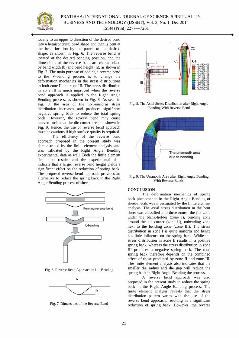
PRATIBHA: INTERNATIONAL JOURNAL OF SCIENCE, SPIRITUALITY,
BUSINESS AND TECHNOLOGY (IJSSBT), Vol. 3, No. 1, Dec 2014
ISSN (Print) 2277—7261
21
locally to an opposite direction of the desired bend
into a hemispherical bead shape and then is bent at
the bead location by the punch to the desired
shape, as shown in Fig. 6. The reverse bend is
located at the desired bending position, and the
dimensions of the reverse bend are characterized
by band width (b) and bend height (h), as shown in
Fig. 7. The main purpose of adding a reverse bend to the V-bending process is to change the
deformation mechanics in the stress distributions
in both zone II and zone III. The stress distribution
in zone III is much improved when the reverse
bend approach is applied to the Right Angle
Bending process, as shown in Fig. 8. As seen in
Fig. 8, the area of the non-uniform stress
distribution increases and produces significant
negative spring back to reduce the total spring
back. However, the reverse bend may cause
uneven surface at the die corner area, as shown in
Fig. 9. Hence, the use of reverse bend approach must be cautious if high surface quality is required.
The efficiency of the reverse bend
approach proposed in the present study was
demonstrated by the finite element analysis, and
was validated by the Right Angle Bending
experimental data as well. Both the finite element
simulation results and the experimental data
indicate that a larger reverse bend height yields a
significant effect on the reduction of spring back.
The proposed reverse bend approach provides an
alternative to reduce the spring back in the Right Angle Bending process of sheets.
Fig. 6. Reverse Bend Approach in L – Bending
Fig. 7. Dimensions of the Reverse Bend
Fig. 8. The Axial Stress Distribution after Right Angle Bending With Reverse Bend
Fig. 9. The Unsmooth Area after Right Angle Bending
With Reverse Bends.
CONCLUSION
The deformation mechanics of spring
back phenomenon in the Right Angle Bending of sheet-metals was investigated by the finite element
analysis. The axial stress distribution in the bent
sheet was classified into three zones: the flat zone
under the blank-holder (zone I), bending zone
around the die corner (zone II), unbending zone
next to the bending zone (zone III). The stress
distribution in zone I is quite uniform and hence
has little influence on the spring back. While the
stress distribution in zone II results in a positive
spring back, whereas the stress distribution in zone
III produces a negative spring back. The total spring back therefore depends on the combined
effect of those produced by zone II and zone III.
The finite element analysis also indicates that the
smaller die radius and die gap will reduce the
spring back in Right Angle Bending the process.
A reverse bend approach was also
proposed in the present study to reduce the spring
back in the Right Angle Bending process. The
finite element analysis reveals that the stress
distribution pattern varies with the use of the
reverse bend approach, resulting in a significant
reduction of spring back. However, the reverse

PRATIBHA: INTERNATIONAL JOURNAL OF SCIENCE, SPIRITUALITY,
BUSINESS AND TECHNOLOGY (IJSSBT), Vol. 3, No. 1, Dec 2014
ISSN (Print) 2277—7261
22
bend approach may cause uneven surface around
the die corner. Hence, the use of the reverse bend
approach must be cautious if the surface quality is
required.
The finite element analysis performed in
the present study was validated by experiments as
well. The good agreement between the finite
element simulation results and the experimental data confirm the efficiency in using the finite
element analysis in the Right Angle Bending
process of sheet-metals.
REFERENCES
[1] W. Schroeder, Mechanics of sheet-metal bending,
Trans ASME 65 (1943) 817-827.
[2] G. Martin, S. Tang, The plastic bending of beams
considering die friction effects, J. Eng. Ind. 88 (1966)
237-250.
[3] T.X. Yu, W. Johnson, Influence of axial force on
elastic plastic bending and spring back of a beam, J.
Mech. Working Tech., 6 (1982) 5-21.
[4] R. Hill, The mathematical theory of plasticity, Oxford
University Press (1950).
[5] R.G. Davies, C.C Chu., Y.C. Liu, Recent progress on
the understanding of spring back, Computer Modeling
of Sheet Metal Forming Process, ed. By N. M. Wang
and S. C. Tang, The Metallurgical Society, USA,
(1985) 259-271.
[6] C.C. Chu, The effect of restraining force on spring
back, Int. J. Solids in Structure, 27 (1991) 1035 -1046.
[7] N. Asnafi, Spring back and fracture in V-die air
bending of thick stainless steel sheets, Material and
Design, 21 (2000) 217-236.
[8] Y.C. Liu, Spring back reduction in U-channels: double-
bend technique, J. App. Metal, 3 (1984) 148-156.
[9] Y. Nagai, High precision U-bending technique for
moderately thick plate, JSTP 28 (1987) 143-149.
[10] C. Wang, G. Kinzel, T. Altan, Mathematical modeling
of plane-strain bending of sheet and plate, J. Mater.
Processing Tech., 39 (1993) 279-304.
[11] K.C. Chan, S.H. Wang, "Theoretical analysis of spring
back in bending of integrated circuit lead frames "
Journal of Materials Processing Technology, 91(1-3)
(1999)111-115.
[12] H. Livatyali, T. Altan, "Prediction and elimination of
spring back in straight flanging using computer aided
design methods: Part 1. Experimental investigations
"Journal of Materials Processing Technology, 117(1-2):
(2001) 262-268.
[13] H.B. Mullan. "Improved prediction of spring back on
final formed components‖ Journal of Materials
Processing Technology 153-154 (2004) 464-471.
[14] L. Papeleux, J.P. Ponthot, "Finite element simulation of
spring back in sheet metal forming‖ Journal of
Materials Processing Technology 125-126 (2002) 785-
791.
[15] M. Samuel, "Experimental and numerical prediction of
spring back and side wall curl in U-bandings of
anisotropic sheet metals " Journal of Materials
Processing Technology 105(3) (2000) 382-393.

PRATIBHA: INTERNATIONAL JOURNAL OF SCIENCE, SPIRITUALITY,
BUSINESS AND TECHNOLOGY (IJSSBT), Vol. 3, No. 1, Dec 2014
ISSN (Print) 2277—7261
23
Computational Fluid Dynamics (CFD) Simulation of Helical
Coil Induction Water Heater using Induction Cooker
Tejas G. Patil1, Atul A. Patil
2, Dheeraj S. Deshmukh
3
1,2,3Deprtment of Mechanical Engineering, Godavari College of Engineering, Jalgaon – 425001, India. 3Deprtment of Mechanical Engineering, SSBT College of Engineering & Technology, Jalgaon – 425001,
India.
Emails: [email protected], [email protected], [email protected]
Abstract: This communication presents a
comparative performance study of helical coil
induction water heater with three, four and five
helical coils through a computational fluid
dynamics (CFD) simulation. Helical coil is
designed and modelled as per selection of one
variable parameters keeping others constant.
Simulations were performed using variable flow
rate of water through helical coil with different
number of turns N=3.25, N=4 and N=5. The
values of water outlet temperature observed
with variable flow rates of water during the
CFD analysis using Fluent software is getting
affected with the help of different helical coil
configurations by changing number of turns
with coil pitch, coil diameter and coil tube
diameter retains constant. The heat supplied to
helical coil from induction cooker which used in
CFD as heat flux on surface of coil. Results
indicated that the water outlet temperature
from helical coil is increases with increase in
number of turns except for N=3.25.
Keywords: Computational Fluid Dynamics
(CFD), Helical Coil, Fluent, Coil Pitch.
I. INTRODUCTION
Helical coils are widely used in
applications such as heat recovery system,
chemical processing, food processing, nuclear
reactors and high-temperature gas cooling reactors
[1]. Because of helical coils have a compact configuration, more heat transfer surface can be
provided per unit of space than by the use of
straight tubes, ease of manufacture and longer
operating life. Industrial demands of electricity and
especially water at certain temperature of 850-900
for different processes to fulfill demands it
required lot of electricity or fuel and also for hot
water required at particular temperature using
different techniques including Electric Heater, Gas
Water Heater, Storage Heat Pump water heater,
Heat Exchanger using burning of fuel etc. Due to deficiency of resources in environment it is
necessary to find out alternative energy resources
or use available resources effectively; so for water
heating process it should aimed at having effective
use over the supplied electricity, the new technique
of water heating using induction heating process is
being developed. Typical applications of induction
heating are melting of metals, heating of metals for
design, Brazing, Welding and all sorts of Surface
Treatments. These process is required to verify results obtained in the experimentation with
software; the tool developed named CFD Fluent
simulation is used.
CFD simulation can be used to study the
fluid flow and heat transfer for a wide variety of
engineering equipment. In this study, we use heat
transfer simulation to analyze the efficiency of
helical coil induction water heater to observe the
water temperature at outlet of helical coil when
certain constant heat supplied form induction
cooker where continuous flow of water from helical coil [2]. With heat transfer simulation the
determination of the efficiency of the system and
water outlet temperature from helical coil with
applying heat flux to it, and design engineer can
gain insight into the physical processes involved,
thus giving guidance for improvements to be
design.
Nihar P Bara (2013), states the main
benefits of using induction processes when
compared to any other heating process (gas
furnace) are among others, their fast heating rate,
good reproducibility, little energy consumption which verified with finite element analysis (FEA)
of induction furnace [3].
The previous work done by Ordoñez
Flores Rafael, Reyes Castillo Fabiola and Carreño
Hernández Carlos (2013) on water heater by
magnetic induction described new device which
projected to heat the shower water as it obeys the
excessive water wasting at start of knob of water,
so it anticipates a water and gas saving. This water
heater consumes not as much of electrical energy
in the resistance based boiler and it doesn‘t store

PRATIBHA: INTERNATIONAL JOURNAL OF SCIENCE, SPIRITUALITY,
BUSINESS AND TECHNOLOGY (IJSSBT), Vol. 3, No. 1, Dec 2014
ISSN (Print) 2277—7261
24
hot water which signifies use of less energy than
the gas based [4].
A review study done by N. D. Shirgire
and P. Vishwanath Kumar (2013), on comparison
of helical coil and straight tube heat exchanger
heat transfer coefficient of helical coil is affected
by geometry of heat exchanger. Helical coils offer
beneficial over straight tubes due to their compactness with improved heat transfer
coefficient. The effectiveness of heat exchanger
greatly affected by hot water mass flow rate and
cold water flow rate. When cold water mass flow
rate is constant and hot water mass flow rate
increases the effectiveness decreases and increase
in cold water mass flow rate for constant hot water
mass flow rate resulted in increase in effectiveness
henceforth flow rate of fluid plays vital role in
experimenting with helical coil [5].
With the above advantages for fluent
simulation; model is being developed with required dimensions in 3D drawing software and
these is utilized in grid generation of solid-fluid
interface to apply heat transfer process. After
meshing of model is used in fluent software to
analyze the heat transfer trough varying boundary
conditions different output can be achieved. In this
work we have find out the water outlet temperature
from helical coil with heat flux applied on it.
II. MODELLING OF HELICAL COIL
The 3D model for each helical coil is
created using CAD Package CATIA V5 R19. It is
imported in Ansys fluent workbench. The extra length added at inlet and outlet of helical turns of
coil which helps in reducing the non-uniformity of
flow. The geometrical specifications of the helical
coil have chosen somewhat arbitrarily. Diameter of
helical coil is D=0.1095m center to center, pitch of
helical coil is P=0.0095 m, helical tube diameter is
d0=0.0095m and thickness 0.5 mm with variable
number of turns ―N‘ is selected as N=3.25, N=4
and N=5.
Extra length added to inlet of helical coil =
130 mm Extra length added at outlet of coil varies with
number of turn selected for simulation purpose is
as follows:
1. For N=3.25 Extra length added to outlet of
helical coil = 75 mm
2. For N=4 Extra length added to outlet of helical
coil = 95 mm
3. For N=5 Extra length added to outlet of helical
coil = 120 mm
Generally these modelled is designed with solid-
fluid interface required for grid generation and
applying heat transfer from solid body to fluid flowing through it as shown in figure 6. The model
of helical coil N=3.25, N=4 and N=5 is shown in
figure 1.
Fig. 1 Model of helical coil N=3.25
Then all the parts are defined i.e. inlet is
defined as Inflow, outlets as Outflow and wall.
III. GRID GENERATION FOR THE
HELICAL COIL WITH SOLID-FLUID
INTERFACE
The ANSYS ICEM-CFD is used for discretization of domain. Initially a relatively
coarser mesh is generated. This mesh contains
tetrahedral cells having triangular faces at the
boundaries. Care is taken to use tetrahedral cells as
much as possible. It is meant to reduce numerical
diffusion as much as possible by structuring the
mesh in a well manner, particularly near the wall
region. Later on, a fine mesh is generated for this
fine mesh, the edges and regions of high
temperature and pressure gradients are finely
meshed which is solid fluid interface.
Table I: Mesh details
Parameter Details
1.Global Mesh Size 10 mm
2. Surface Mesh Size 10 mm
3. Curve Mesh Size 10 mm
4.Mesh Type tetrahedral
5.No.of Elements 430767
6.Mesh Quality 0.4
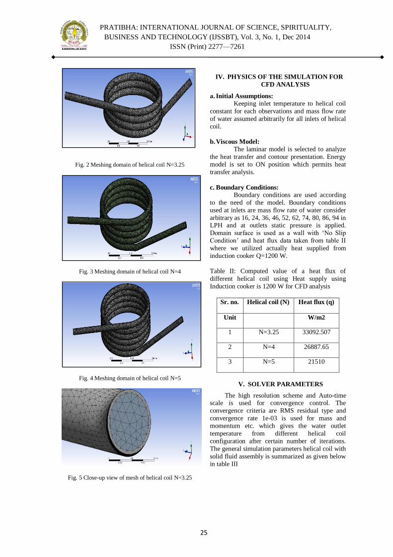
PRATIBHA: INTERNATIONAL JOURNAL OF SCIENCE, SPIRITUALITY,
BUSINESS AND TECHNOLOGY (IJSSBT), Vol. 3, No. 1, Dec 2014
ISSN (Print) 2277—7261
25
Fig. 2 Meshing domain of helical coil N=3.25
Fig. 3 Meshing domain of helical coil N=4
Fig. 4 Meshing domain of helical coil N=5
Fig. 5 Close-up view of mesh of helical coil N=3.25
IV. PHYSICS OF THE SIMULATION FOR
CFD ANALYSIS
a. Initial Assumptions:
Keeping inlet temperature to helical coil
constant for each observations and mass flow rate
of water assumed arbitrarily for all inlets of helical
coil.
b. Viscous Model:
The laminar model is selected to analyze
the heat transfer and contour presentation. Energy
model is set to ON position which permits heat
transfer analysis.
c. Boundary Conditions:
Boundary conditions are used according
to the need of the model. Boundary conditions
used at inlets are mass flow rate of water consider
arbitrary as 16, 24, 36, 46, 52, 62, 74, 80, 86, 94 in LPH and at outlets static pressure is applied.
Domain surface is used as a wall with ‗No Slip
Condition‘ and heat flux data taken from table II
where we utilized actually heat supplied from
induction cooker Q=1200 W.
Table II: Computed value of a heat flux of
different helical coil using Heat supply using
Induction cooker is 1200 W for CFD analysis
Sr. no. Helical coil (N) Heat flux (q)
Unit W/m2
1 N=3.25 33092.507
2 N=4 26887.65
3 N=5 21510
V. SOLVER PARAMETERS
The high resolution scheme and Auto-time scale is used for convergence control. The
convergence criteria are RMS residual type and
convergence rate 1e-03 is used for mass and
momentum etc. which gives the water outlet
temperature from different helical coil
configuration after certain number of iterations.
The general simulation parameters helical coil with
solid fluid assembly is summarized as given below
in table III

PRATIBHA: INTERNATIONAL JOURNAL OF SCIENCE, SPIRITUALITY,
BUSINESS AND TECHNOLOGY (IJSSBT), Vol. 3, No. 1, Dec 2014
ISSN (Print) 2277—7261
26
Table III: Details of simulation
Parameter Ansys Fluent
Domain of
simulation
Helical coil with solid
liquid interface
Laminar model Viscous
Heat Transfer
model
Thermal Energy
Fluid Water
Solid Steel
Reference Pressure 1 atm.
Inlet Mass flow rate and
Temperature of Fluid
Outlet Static pressure
Discretization High Resolution
Residual Type RMS
Residual Target 1e-03
Fig. 6 FLUENT simulation model of helical coil N=3.25
VI. RESULTS AND DISCUSSION
Fig. 7 Variation in water outlet temperature vs. water flow rate for different helical coil N=3.25, N=4 and N=5
using CFD fluent
It is observed from the figure 7 variation in
water outlet temperature Vs. water flow rate for
different helical coil N=3.25, N=4 and N=5 using
CFD fluent that when one helical coil is selected at
different water flow rate viz. 16 LPH to 94 LPH
the water outlet temperature using CFD fluent
decreases with increase in water flow rates. During
the change of helical coil as number of turns increases form N=3.25 to N=5 value of water
outlet temperature using CFD is also increased at
particular water flow rate. Water outlet
temperature of helical coil N=3.25 is found to be
maximum among different coil configurations
available at particular flow rate and it decreases in
helical coil N=4 and rise again for helical coil N=5
as number of turns of coil increases.
VII. CONCLUSIONS
It is concluded from Computational Fluid
Dynamics (CFD) simulation using Fluent as number of turns of helical coil is increases the
water outlet temperature also increases at constant
flow rates keeping other parameters constant. This
heat is supplied through induction cooker which is
contactless, pollution free and safety for water
heating process. Using CFD simulation variable
parameter can be optimized to design helical coil
which gives maximum water outlet temperature
which is being utilized in industry for continuous
requirement.
REFERENCES
[1] C.A. Chaves, D.R.F. de Castro, W.Q. Lamas, J.R.
Camargo and F.J. Grandinetti (2014): Computational
Fluid Dynamics (CFD) Simulation to Analyze the
Performance of Tube-in-Tube helically coiled of a Heat
Exchanger, Academics Journals, Vol. 9(7), 15 April
2014, pp. 181-188
[2] Tejas G. Patil and Atul A. Patil (2014): Experimental
Study of Helical Coil Induction Water Heater Using
Induction Cooker, International Journal of Research in
Aeronautical and Mechanical Engineering, Vol. 2,
Issue 7, July 2014, PP 21-27
[3] Nihar P Bara (2013): Finite Element Analysis of
Induction Furnace for Optimum Heat Transfer,
International Journal of Innovative Research in
Science, Engineering and Technology, Vol. 2, Issue 5,
May 2013. PP 1313-1319.
[4] Ordoñez Flores Rafael, Reyes Castillo Fabiola and
Carreño Hernández Carlos (2013): Water Heater by
Magnetic Induction, 978-1-4673-6155-2/13 2013 IEEE
Journal
[5] N. D. Shirgire, and P. Vishwanath Kumar (2013):
Review on Comparative Study between Helical Coil
and Straight Tube Heat Exchanger, IOSR Journal of
Mechanical and Civil Engineering (IOSR-JMCE).
Volume 8, Issue 2 (Jul. - Aug. 2013), PP 55-59.

PRATIBHA: INTERNATIONAL JOURNAL OF SCIENCE, SPIRITUALITY,
BUSINESS AND TECHNOLOGY (IJSSBT), Vol. 3, No. 1, Dec 2014
ISSN (Print) 2277—7261
27
Materials Selection Criteria for Thermoelectric Power
Generators Performance Enhancement: A Critical Review
P. M. Solanki Assistant Professor, Mechanical Engineering, SSBT`s COET, Bambhori, (M. S.), India
Email: [email protected]
Dr. D.S. Deshmukh Professor & Head, Mechanical Engineering, SSBT`s COET, Bambhori, (M. S.), India
Email: [email protected]
ABSTRACT: World from the last few years
facing difficulties regarding energy
management, energy consumption and sources
of energy like renewable and non renewable,
are insufficient in comparison of the future
energy trends. This is not only due to world
population but also a long range of electrical
and electronics based demands of modern life
are responsible for it. These all causes the world
that leads to the need of introduction of some
techniques, modifications, nuclear power plants
and nano cells to overcome the energy crisis.
Thermoelectric modules playing an important
role by the conversion of waste heat into
electricity. The implementation of
thermoelectric devices with cheap, single step
power generation and without any pollution can
be considered as key factors to green energy
generations. In such regions the thermoelectric
generators can be used to produce adequate
amount of power like heat of stoves, wood, daily
wastage. Such issues are also come into picture
in engineering fields due to large scale
consumption of energy and low efficiency of
modern high facilitated devices. Attempts are
also being made to improve the competitiveness
of thermoelectric generators in directions other
than by improving the figure-of-merit for
materials. In particular, efforts are focused on
increasing the electrical power factor,
decreasing cost and developing environmental
friendly materials. In addition to this the fuel
cost is low or free as in waste heat recovery
systems using thermoelectric generator. The
cost per unit power generation is mainly
determined by the power per unit area and
operating period. Thus in this paper all
desirable properties of good materials for
thermoelectric generators are discussed.
KEYWORDS: Thermoelectric power generation,
Waste-heat recovery, Alternative green
technology, Direct energy conversion, Electrical
power, Thermoelectric materials.
I. INTRODUCTION:
Thermoelectric (TE) devices create electricity from
a thermal gradient or create a thermal gradient
from electricity via the thermoelectric effect. This phenomenon comprises three related effects,
uncovered as a series of discoveries made
primarily by Thomas Johann Seebeck, Jean-
Charles Peltier, and William Thomson (Lord
Kelvin) in the 19th century[1]. The Seebeck effect
asserts that a potential gradient will be created
across a conducting material when one side of the
material is hotter than the other. In reality, charge
carriers (electrons and holes) in the material having
higher thermal velocities on the hot side of the
material naturally diffuse more quickly from the hot side to the cold side than in the opposite
direction. If the thermal gradient across the
material is maintained, flowing charge carriers
build up on the cold side of the object, and this
separation of charge creates a potential difference
between the two sides of the material which
counters this charge imbalance. In the case that the
material is part of a circuit, this voltage induces a
current which be used to power a load [1]. Figure1
illustrated a conductor under a thermal gradient,
charge carriers (electrons in this case) on the hot
side have higher thermal velocities, diffusing more quickly to the cold side of the material than
electrons on the cold side diffuse to the hot side.
This leaves an excess of carriers on the cold side,
and a potential gradient and electric field are
created across the material[2] and essentially
constitutes a conversion of thermal energy to
electricity. The potential difference created per
degree of temperature gradient across the material
is its Seebeck coefficient, S, and is material-
dependent [1].
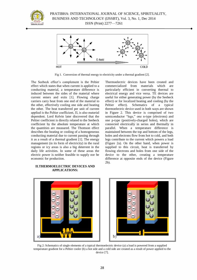
PRATIBHA: INTERNATIONAL JOURNAL OF SCIENCE, SPIRITUALITY,
BUSINESS AND TECHNOLOGY (IJSSBT), Vol. 3, No. 1, Dec 2014
ISSN (Print) 2277—7261
28
Fig 1. Conversion of thermal energy to electricity under a thermal gradient [2].
The Seebeck effect‘s complement is the Peltier
effect which states that when current is applied to a
conducting material, a temperature difference is induced between the sides of the material where
current enters and exits [1]. Flowing charge
carriers carry heat from one end of the material to
the other, effectively cooling one side and heating
the other. The heat transferred per unit of current
applied is the Peltier coefficient, Π, is also material
dependent. Lord Kelvin later discovered that the
Peltier coefficient is directly related to the Seebeck
coefficient by the absolute temperature at which
the quantities are measured. The Thomson effect
describes the heating or cooling of a homogeneous conducting material due to current passing through
it as a result of a thermal gradient [1]. The energy
management (in its form of electricity) in the rural
regions or icy areas is also a big deterrent in the
daily life activities. In some of these areas the
electric power is neither feasible to supply nor be
economic for production.
II.THERMOELECTRIC DEVICES AND
APPLICATIONS:
Thermoelectric devices have been created and
commercialized from materials which are
particularly efficient in converting thermal to electrical energy and vice versa. TE devices are
useful for either generating power (by the Seebeck
effect) or for localized heating and cooling (by the
Peltier effect). Schematics of a typical
thermoelectric device used in both ways are shown
in Figure 2. This device is comprised of two
semiconductor ―legs,‖ one n-type (electrons) and
one p-type (positively-charged holes), which are
connected electrically in series and thermally in
parallel. When a temperature difference is
maintained between the top and bottom of the legs, holes and electrons flow from hot to cold, and both
legs contribute to the current which powers a load
(Figure 2a). On the other hand, when power is
supplied to this circuit, heat is transferred by
flowing electrons and holes from one side of the
device to the other, creating a temperature
difference at opposite ends of the device (Figure
2b).
Fig 2: Schematics of single elements of a typical thermoelectric device (a) a load is powered from a supplied temperature gradient for a Peltier cooler (b) a hot side and a cold side are created as a result of power applied to the
device [7].
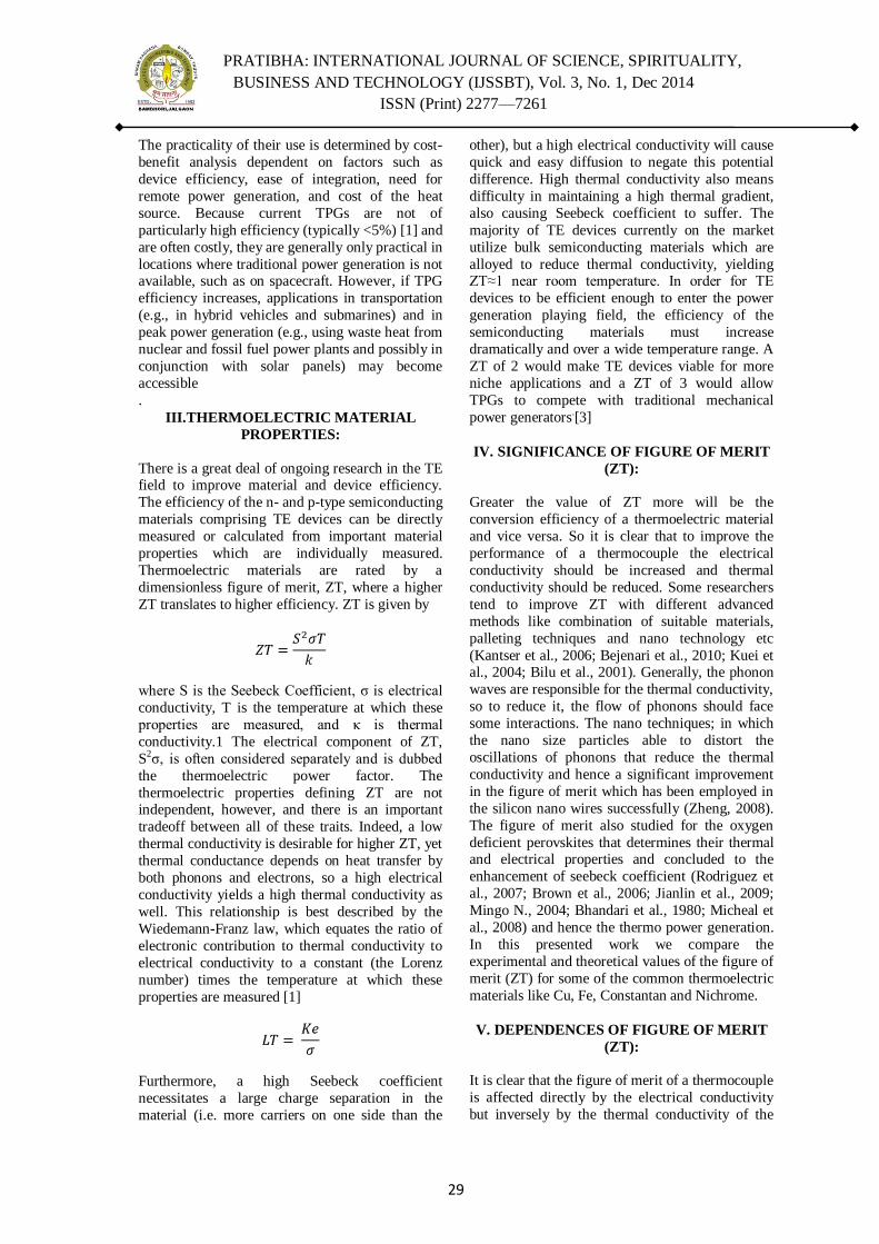
PRATIBHA: INTERNATIONAL JOURNAL OF SCIENCE, SPIRITUALITY,
BUSINESS AND TECHNOLOGY (IJSSBT), Vol. 3, No. 1, Dec 2014
ISSN (Print) 2277—7261
29
The practicality of their use is determined by cost-
benefit analysis dependent on factors such as
device efficiency, ease of integration, need for
remote power generation, and cost of the heat
source. Because current TPGs are not of
particularly high efficiency (typically <5%) [1] and
are often costly, they are generally only practical in
locations where traditional power generation is not available, such as on spacecraft. However, if TPG
efficiency increases, applications in transportation
(e.g., in hybrid vehicles and submarines) and in
peak power generation (e.g., using waste heat from
nuclear and fossil fuel power plants and possibly in
conjunction with solar panels) may become
accessible
.
III.THERMOELECTRIC MATERIAL
PROPERTIES:
There is a great deal of ongoing research in the TE field to improve material and device efficiency.
The efficiency of the n- and p-type semiconducting
materials comprising TE devices can be directly
measured or calculated from important material
properties which are individually measured.
Thermoelectric materials are rated by a
dimensionless figure of merit, ZT, where a higher
ZT translates to higher efficiency. ZT is given by
where S is the Seebeck Coefficient, σ is electrical
conductivity, T is the temperature at which these
properties are measured, and κ is thermal
conductivity.1 The electrical component of ZT,
S2σ, is often considered separately and is dubbed
the thermoelectric power factor. The
thermoelectric properties defining ZT are not independent, however, and there is an important
tradeoff between all of these traits. Indeed, a low
thermal conductivity is desirable for higher ZT, yet
thermal conductance depends on heat transfer by
both phonons and electrons, so a high electrical
conductivity yields a high thermal conductivity as
well. This relationship is best described by the
Wiedemann-Franz law, which equates the ratio of
electronic contribution to thermal conductivity to
electrical conductivity to a constant (the Lorenz
number) times the temperature at which these
properties are measured [1]
Furthermore, a high Seebeck coefficient
necessitates a large charge separation in the
material (i.e. more carriers on one side than the
other), but a high electrical conductivity will cause
quick and easy diffusion to negate this potential
difference. High thermal conductivity also means
difficulty in maintaining a high thermal gradient,
also causing Seebeck coefficient to suffer. The
majority of TE devices currently on the market
utilize bulk semiconducting materials which are
alloyed to reduce thermal conductivity, yielding ZT≈1 near room temperature. In order for TE
devices to be efficient enough to enter the power
generation playing field, the efficiency of the
semiconducting materials must increase
dramatically and over a wide temperature range. A
ZT of 2 would make TE devices viable for more
niche applications and a ZT of 3 would allow
TPGs to compete with traditional mechanical
power generators.[3]
IV. SIGNIFICANCE OF FIGURE OF MERIT
(ZT):
Greater the value of ZT more will be the
conversion efficiency of a thermoelectric material
and vice versa. So it is clear that to improve the
performance of a thermocouple the electrical
conductivity should be increased and thermal
conductivity should be reduced. Some researchers
tend to improve ZT with different advanced
methods like combination of suitable materials,
palleting techniques and nano technology etc
(Kantser et al., 2006; Bejenari et al., 2010; Kuei et al., 2004; Bilu et al., 2001). Generally, the phonon
waves are responsible for the thermal conductivity,
so to reduce it, the flow of phonons should face
some interactions. The nano techniques; in which
the nano size particles able to distort the
oscillations of phonons that reduce the thermal
conductivity and hence a significant improvement
in the figure of merit which has been employed in
the silicon nano wires successfully (Zheng, 2008).
The figure of merit also studied for the oxygen
deficient perovskites that determines their thermal and electrical properties and concluded to the
enhancement of seebeck coefficient (Rodriguez et
al., 2007; Brown et al., 2006; Jianlin et al., 2009;
Mingo N., 2004; Bhandari et al., 1980; Micheal et
al., 2008) and hence the thermo power generation.
In this presented work we compare the
experimental and theoretical values of the figure of
merit (ZT) for some of the common thermoelectric
materials like Cu, Fe, Constantan and Nichrome.
V. DEPENDENCES OF FIGURE OF MERIT
(ZT):
It is clear that the figure of merit of a thermocouple
is affected directly by the electrical conductivity
but inversely by the thermal conductivity of the

PRATIBHA: INTERNATIONAL JOURNAL OF SCIENCE, SPIRITUALITY,
BUSINESS AND TECHNOLOGY (IJSSBT), Vol. 3, No. 1, Dec 2014
ISSN (Print) 2277—7261
30
thermoelectric material. (a) The thermal
conductivity of a material is the ease with which
the heat flows through itself and its expression
from literature is given by:
Where, is the rate of heat flow, is the
temperature gradient, is the time for which the
heat flow, A is the area of cross section of the
thermoelectric materials with thickness x.(b) The
electrical conductivity of a thermoelectric material
is the ease of the material to allow the passage of electric current and is given by
Where R is the resistance of thermoelectric
material in ohms, and where is the
resistivity (specific resistance) of the material in
Ωm, l and A are the length and area of cross-
section of the material respectively.
VI.THERMOELECTRIC POWER
GENERATOR PERFORMANCE
CALCULATION:
The performance of the thermoelectric
calculation[8]
Where Z = Thermoelectric material figure of Merit
= See back Coefficient is given by
= temperature difference
R is the electric resistivity
K is the thermal conductivity This figure of merit can be multiplied by T average
absolute temperature of hot and cold platesof the
thermoelectric module, K
Here
T= TH + TL/2
Where TH = Temperature at hot End
TL = Temperature at cold end
See back Coefficient
By the second law of thermodynamics, the ideal
(absolute maximum efficiency of the
thermoelectric power generator operating as a
reversible heat engine is Carnot efficiency
η = We/QH
ηcarnot= 1-TL/TH
The maximum conversion efficiency of an
irreversible power generator can be estimated
using
VII. THERMOELECTRCI MATERIALS FOR
POWER GENERATORS:
Among the vast number of materials known to
date, only a relatively few are identified as
thermoelectric materials. As reported by Rowe [4],
thermoelectric materials can be categorized into
established (conventional) and new (novel)
materials. Today's most thermoelectric materials,
such as Bismuth Telluride (Bi2Te3)-based alloys
and PbTe-based alloys, have a ZT value of around unity (at room temperature for Bi2Te3 and 500-
700K for PbTe). However, at a ZT of 2-3 range,
thermoelectric power generators would become
competitive with other power generation systems.
The figure-of- merit Z of a number of
thermoelectric materials together
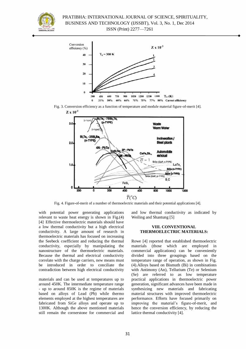
PRATIBHA: INTERNATIONAL JOURNAL OF SCIENCE, SPIRITUALITY,
BUSINESS AND TECHNOLOGY (IJSSBT), Vol. 3, No. 1, Dec 2014
ISSN (Print) 2277—7261
31
Fig. 3. Conversion efficiency as a function of temperature and module material figure-of-merit [4].
Fig. 4. Figure-of-merit of a number of thermoelectric materials and their potential applications [4].
with potential power generating applications
relevant to waste heat energy is shown in Fig.(4)
[4]. Effective thermoelectric materials should have
a low thermal conductivity but a high electrical
conductivity. A large amount of research in
thermoelectric materials has focused on increasing
the Seebeck coefficient and reducing the thermal
conductivity, especially by manipulating the
nanostructure of the thermoelectric materials.
Because the thermal and electrical conductivity
correlate with the charge carriers, new means must
be introduced in order to conciliate the contradiction between high electrical conductivity
and low thermal conductivity as indicated by
Weiling and Shantung [5]
VIII. CONVENTIONAL
THERMOELECTRIC MATERIALS:
Rowe [4] reported that established thermoelectric
materials (those which are employed in
commercial applications) can be conveniently
divided into three groupings based on the
temperature range of operation, as shown in Fig.
(4).Alloys based on Bismuth (Bi) in combinations with Antimony (An), Tellurium (Te) or Selenium
(Se) are referred to as low temperature
materials and can be used at temperatures up to
around 450K. The intermediate temperature range
- up to around 850K is the regime of materials
based on alloys of Lead (Pb) while thermo
elements employed at the highest temperatures are
fabricated from SiGe alloys and operate up to
1300K. Although the above mentioned materials
still remain the cornerstone for commercial and
practical applications in thermoelectric power
generation, significant advances have been made in
synthesizing new materials and fabricating
material structures with improved thermoelectric
performance. Efforts have focused primarily on
improving the material‘s figure-of-merit, and
hence the conversion efficiency, by reducing the
lattice thermal conductivity [4].

PRATIBHA: INTERNATIONAL JOURNAL OF SCIENCE, SPIRITUALITY,
BUSINESS AND TECHNOLOGY (IJSSBT), Vol. 3, No. 1, Dec 2014
ISSN (Print) 2277—7261
32
IX. NOVEL THERMOELECTRIC
MATERIALS & MODULE
CONFIGURATION:
It was recently reported in [6] that a material which
is a promising candidate to fill the temperature
range in the ZT spectrum between those based on Bi2Te3 and PbTe is the semiconductor compound
ß-Zn4Sb3. This material possesses an exceptionally
low thermal conductivity and exhibits a maximum
ZT of 1.3 at a temperature of 670K. This material
is also relatively inexpensive and stable up to this
temperature in a vacuum [6]. Another recent
direction to improve the competitiveness of
thermoelectric materials, other than by improving
the figure-of-merit, is by developing novel
thermoelectric module shapes.
X. CONCLUSION:
Study of thermoelectric materials selection criteria
indicates that efficiency of the thermoelectric
generator depends upon the figure of merit for
materials, is key consideration for comparing the
efficiency of thermoelectric materials. It is
observed that most commonly used thermoelectric
materials, are Cu, Fe, Constantan and Nichrome,
Bismuth Telluride (Bi2Te3)-based alloys and Lead
Telluride (PbTe)-based alloys. Effective
thermoelectric materials should have a low thermal conductivity but a high electrical conductivity. A
lot of research in thermoelectric materials is
focused on increasing the Seebeck coefficient and
reducing the thermal conductivity, especially by
manipulating nanostructure of thermoelectric
materials.
ACKNOWLEDGEMENT
Authors would like to thanks RGS&TC grants
received through North Maharashtra University Jalgaon for providing financial support and
SSBT‘s,COET, Bambhori, Jalgaon, (M. S.), India
for providing library facility.
REFRENCES
[1] D. M. Rowe, ed., CRC Handbook of Thermoelectrics.
CRC Press (1995).
[2] J. M. O. Zide, ―Molecular Beam Epitaxial Growth of III-
V Semimetal/III-V Semiconductor Nanocomposites for
Energy Conversion Applications,‖ PhD dissertation,
University of California, Santa Barbara (2007).
[3] C. J. Vineis, A. Shakouri, A. Majumdar, and M. G.
Kanatzidis, ―Nanostructured Thermoelectrics: Big
Efficiency Gains from Small Features,‖ Advanced
Matererials 22, 3970-0980 (2010).
[4] Rowe D. M. Thermoelectric waste heat recovery as a
renewable energy source. Int J Innov Energy Syst Power
2006; 1: 13-23.
[5] Weiling L, Shantung TU. Recent developments of
thermoelectric power generation. Chin Sci Bull 2004;
49(12): 1212-1219.
[6] Rowe D.M, Min G. Evaluation of thermoelectric modules
for power generation. J Power Sources 1998; 73: 193-198.
[7] Ling Xu, Yuchun Liu, Bingbing Chen, Chen Zhao, Kai Lu
,Wu Han ―Enhancement in Thermoelectric Properties
Using a P-type and N-type Thin-Film Device Structure‖
National Laboratory for Optoelectronics, Huazhong
University of Science and Technology, Wu Han 430074,
China.
[8] P. M. Solanki, Dr. Dheeraj S. Deshmukh and Dr. K. S.
Patil, presented paper at International Conference on
Sustainable Development 2014, titled ―Energy Recovery
using Thermoelectric Generators: A critical Review‖
organized by S.S.B.T.‘s, College of Engineering &
Technology, Bambhori, Jalgaon, on dated 25th- 26
th
February 2014 page no. 80-90.
PRATIBHA: INTERNATIONAL JOURNAL OF SCIENCE, SPIRITUALITY,
BUSINESS AND TECHNOLOGY (IJSSBT), Vol. 3, No. 1, Dec 2014
ISSN (Print) 2277—7261
33
Experimental Verification and CFD Analysis of Single
Cylinder Four Strokes C.I. Engine Exhaust System
Atul A. Patil1,L.G. Navale
2,V.S. Patil
3
1(Research student, North Maharashtra University, Umavi Nagar, Jalgaon, (M. S.) India) 2(Research guide, North Maharashtra University,Umavi Nagar, Jalgaon, (M. S.) India) 3(Research guide, North Maharashtra University,Umavi Nagar, Jalgaon, (M. S.) India) [email protected], [email protected], [email protected]
Abstract: The more amount of air pollution is
due to emissions from an internal combustion
engine. Exhaust system plays a vital role in
reducing harmful gases but the presence of
after treatment systems increases the exhaust
back pressure. To analyse the exhaust energies
available at different engine operating
conditions and to develop an exhaust system for
maximum utilization of available energy at the
exhaust of engine cylinder is studied. Design of
each device should offer minimum pressure
drop across the device, so that it should not
adversely affect the engine performance.
This paper deals with the exhaust system
designed and through CFD (Fluent) analysis, a
compromise between two parameters namely,
more maximisation of brake thermal efficiency
with limited back pressure was aimed at. In
CFD analysis, three exhaust diffuser system
(EDS) models with different angels are
simulated using the appropriate boundary
conditions and fluid properties specified to the
system with suitable assumptions. The back
pressure variations in three models are
discussed in. Finally, the model with limited
backpressure was fabricated and Experiments
are carried out on single cylinder four stroke
diesel engine test rig with rope brake
dynamometer. CFD analysis of exhaust diffuser
systems and the performance of the engine are
discussed.
Keywords: Exhaust Diffuser system (EDS),
Computational Fluid Dynamics (CFD),
Backpressure, Fuel Consumption.
1. Introduction
The exhaust system of an I.C. engine has
significant influence on the global engine
operation. Among the different component of the
system the exhaust system is having paramount relevance on the gas exchange process. Though the
intake system is dominant on the cylinder filling
process, the exhaust system is capable to influence
the gas exchange process in several aspects, like
the piston work during the exhaust stroke, the
short-circuit of fresh charge from the intake into
the exhaust and even the filling of the cylinder. In
this sense, the most influential boundary condition
imposed by the exhaust system is the pressure at
the valve and especially the instantaneous pressure evolution. The mean backpressure is determined
mainly by the singular elements, such as the
turbocharger, the catalytic converter and the
silencer. The instantaneous pressure evolution
imposed by the exhaust system at the exhaust
valve depends essentially on the layout and
dimensions of the pipes, therefore an adequate
design of the exhaust system geometry can
improve the engine power and efficiency, and
reduce the emissions of pollutants.
To reduce the exhaust emissions from C.I.
engines, it is very important to understand the overall effects of devices installed in the exhaust
system. Effective utilization of exhaust energy is
economically possible to reduce exhaust emissions
from old engines instead of engine and fuel
modifications. More efforts are required on the
development of the aftertreatment devices, by
further study of the theory of operation for diesel
engines. Favourable operating parameters
providing in the after-treatment devices during the
whole operating range of the engine requires
proper design of after-treatment devices by considering overall effects of its installation, in the
exhaust system. Obtaining economically,
maximum conversion efficiency of the pollutants
without adversely affecting the engine
performance with durability is the ideal
requirement from the after treatment devices.
Backpressure on engine cylinder is
completely dependent on exhaust system design,
its operating condition and atmospheric pressure
(i.e. almost constant). The exhaust system routes
exhaust gas from the engine and then exhaust it
into the environment, while providing noise attenuation, after treatment of the exhaust gas to
reduce emissions and energy recovery. One of the
most important sources of vehicle noise, the noise

PRATIBHA: INTERNATIONAL JOURNAL OF SCIENCE, SPIRITUALITY,
BUSINESS AND TECHNOLOGY (IJSSBT), Vol. 3, No. 1, Dec 2014
ISSN (Print) 2277—7261
34
associated with exhausting combustion gases from
the engine, is controlled using mufflers. A number
of sound reduction techniques are employed in
mufflers, including reactive silencing, resistive
silencing, absorptive silencing, and shell damping.
Exhaust gas properties which are important for the
exhaust system design include its physical
properties; exhaust gas temperature, which depends on the vehicle duty and/or test cycle and
the exhaust gas flow rate. Exhaust system
materials are exposed to a variety of harsh
conditions, and must be resistant to such
degradation mechanisms as high temperature
oxidation, condensate and salt corrosion, elevated
temperature mechanical failure, stress corrosion
cracking, and inter granular corrosion.
During the exhaust stroke when the piston
moves from BDC to TDC, pressure rises and gases
are pushed into exhaust pipe. Thus the power
required to drive exhaust gases is called exhaust stroke loss and increase in speed increases the
exhaust stroke loss. The network output per cycle
from the engine is dependent on the pumping work
consumed, which is directly proportional to the
backpressure. To minimise the pumping work,
backpressure must be low as possible. The
backpressure is directly proportional to the exhaust
diffuser system design.The shape of the inlet cone
of exhaust diffuser system contributes the
backpressure. This increase in backpressure causes
increase in fuel consumption. Indeed, an increased pressure drop is a very important challenge to
overcome. [1], [2]
2. Causes, Effects and Possible Remedies for
Backpressure Rise Problem
To minimize the pumping work the backpressure
must be as low as possible for obtaining the
optimal output from the engine. The backpressure
is directly proportional to the pressure drop across
the design of complete exhaust system components. Each alternation in exhaust system
causes variations in backpressure on C.I. engine.
There are various factors because of which
backpressure rise problem exists in old as well as
new properly designed C.I. engine applications
during complete operating life. Few of them are
discussed here - An increased C.I. engine
population has created pressures on controlling
engine out emissions. In most of the C.I. engine
applications lack of space availability needs
compactness of after treatment devices, it creates
restriction in exhaust flow hence causes backpressure rise. Diesel after treatment strategies
may include muffler, particulate filter or catalytic
converter, thermal reactor, turbocharger, EGR
system etc. in the exhaust system for heat recovery
and emission control activities. Particulate filters
are designed to trap particulate matter (PM) to
achieve a net decrease in PM emissions. The
device captures ash, but the accumulation of ash in
the device is sufficient to cause a rise in
backpressure. In practice, these devices need to be
regenerate quickly and relatively cheaply when
they become blocked. The failure of catalyst may be due to system component meltdown, carbon
deposit, catalyst fracture, deactivation of diesel
catalyst etc. Aftertreatment device component
failure may cause backpressure rise, mostly it
happens because particulate matter consists of non-
combustible compounds. Poor engine performance
may happen as a result of a clogged or choked
after treatment device. The broken pieces can
move around and get in position to plug up the
flow of exhaust through the device. They are just
melted enough and reduce surface area. Either
way, it doesn‘t work much anymore, even though it may look good on the outside. Engine emissions
increase as the engine deteriorates. Normal engine
wear typically causes an increase of particulate
matter (PM) emissions and a decrease of NOx
emissions. The major categories of fuel additives
include engine performance, fuel handling, fuel
stability, and contaminant control additives.
Engine lubricants are composed of base oil,
viscosity modifier and an additive package. One of
the main drivers in the development of oil
formulations for engines with exhaust aftertreatment is the reduction of sulphated ash,
phosphorous and sulphur. Sulphur increases PM in
all classes of engines. Sulphur is also known to
interfere with several engine emission control
strategies. Development of alternative fuels once
promoted by the desire to reduce exhaust
emissions is now increasingly driven by climate
change issues and energy security. There is a clear
correlation between some fuel properties and
regulated emissions. Drawing general conclusions
is, however, difficult due to such factors as Inter corelation of different fuel properties, different
engine technologies, or engine test cycles. Hence a
comprehensive and practically feasible approach is
a must to improve the complex system of after
treatment. Thus, any modification in engine system
causes rise in backpressure on engine in internal
combustion engines. As a remedial action for
modern internal combustion engine performance
enhancement through controlling the rise in
backpressure following points must be considered.
The regeneration technique employed must be
easy, quick and economic activity. Particulate filters should be installed with backpressure
monitors that would alert the operator when the
backpressure exceeds some pre-set level. With
some insight into the state of the particulate filter

PRATIBHA: INTERNATIONAL JOURNAL OF SCIENCE, SPIRITUALITY,
BUSINESS AND TECHNOLOGY (IJSSBT), Vol. 3, No. 1, Dec 2014
ISSN (Print) 2277—7261
35
(PF), the operator can avoid potentially costly
failures. Some active systems may collect and
store PM over the course of a full day or shift and
can be regenerated at the end of the day or shift
with the vehicle or equipment shut off. A number
of the filters used in stationary like applications
operator can be trained to remove and regenerate
externally at a ―regeneration station‖ for achieving complete regeneration with ease. Because they can
have control over their regeneration and may not
be much dependent on the heat carried in the
exhaust. Careful analysis of application
environment and more stress is required for the
fulfillment of durability requirements, mainly on
catalyst reactivation or replacement techniques
development.[10]
3. Criteria for Design and Development of
Exhaust System
During past studies, more stress has been given to
engine design aspects of Compression Ignition
engines for their performance analysis. Enhance
design, operational and maintenance aspects
specifically related to C.I. engine exhaust system
that is backpressure on engine, needs to be
focused. Backpressure on engine is the pressure
that tries to force the exhaust back in to the engine.
In extreme cases too much backpressure can
damage the engine. In most of literature reviewed
back pressure rise is a common phenomenon observed for after-treatment strategies utilization in
exhaust system of C.I. engines. Possible causes
and their remedies required to be controlled for
exhaust backpressure phenomenon plays vital role,
so this work would be useful for automotive sector
to understand this important controllable
backpressure as an engine operating variable. All
the feasible ways are to be studied for keeping the
backpressure value at minimum level, irrespective
of engine type and operating conditions.
Finally it is decided to have an experimental investigation for energy efficient
exhaust diffuser system design and development
for C.I. engine performance enhancement in the
following manner. In this complete process, three
crucial steps viz. planning, operation and data
analysis should be adopted, in experimental
planning step study of instruments to be used for
precision and accuracy errors should be done.[3]
4. Methodology
The analysis has been carried out on three designs an existing one that is EDS – I with 0° inlet cone
angle, EDS – II with 45° inlet cone angle and a
modified one that is EDS – III with 90° inlet cone
angle, results are subsequently compared. It was
observed that the brake thermal efficiency
improved drastically upon modification in exhaust
geometry. Physical models of the same these two
systems are subsequently manufactured and
exhaustive experiments are carried out on them.
The results obtained through CFD analysis are
experimentally confirmed.
In CFD analysis two major flow characteristics back pressure and engine
performance are studied.
Study I: The change in pressure of structure was
studied. This study offered to find the change in
pressure difference in inlet and outlet of exhaust
diffuser system. The models which produce the
higher pressure difference are selected for further
studies.
Study II: The models which had the higher
pressure difference are studied for the flow pattern.
The back- pressure characteristics of the models are modelled and the model having the lesser
backpressure was taken for experimental analysis
of engine performance. [4]
5. Three Dimensional CFD Study
A three- dimensional model of exhaust diffuser
system is generated in CFD Fluent for the analysis.
A. Modelling and Meshing
The geometry of the element is made as tetrahedral mesh, with a refined mesh near the wall. The K-E
turbulence model is used, with standard wall
functions for near-wall treatment for analysis of
Exhaust system.
B. Boundary Conditions:
Boundary conditions used at inlets mass flow rates
and Temperatures of Fluid are applied and at
outlets pressure outlet is applied. Domain surface
is used as a wall with ‗No Slip condition‘ and heat
transfer coefficient of 45 w/m2 ºk and wall surface roughness as 0.00508 mm is used. [5]
6. CFD Results and Discussion
The primary aim of this CFD analysis is
to find out the right shape of catalytic converter for
the exhaust manifold which can offer minimum
back pressure.[6]
It is observed that the back pressure at
inlet of EDS- I is found to be 1659 Pa, as shown in
Figure 1and 2. The back pressure is found to be
increase with the increase in length of EDS for the
same inlet pressure.
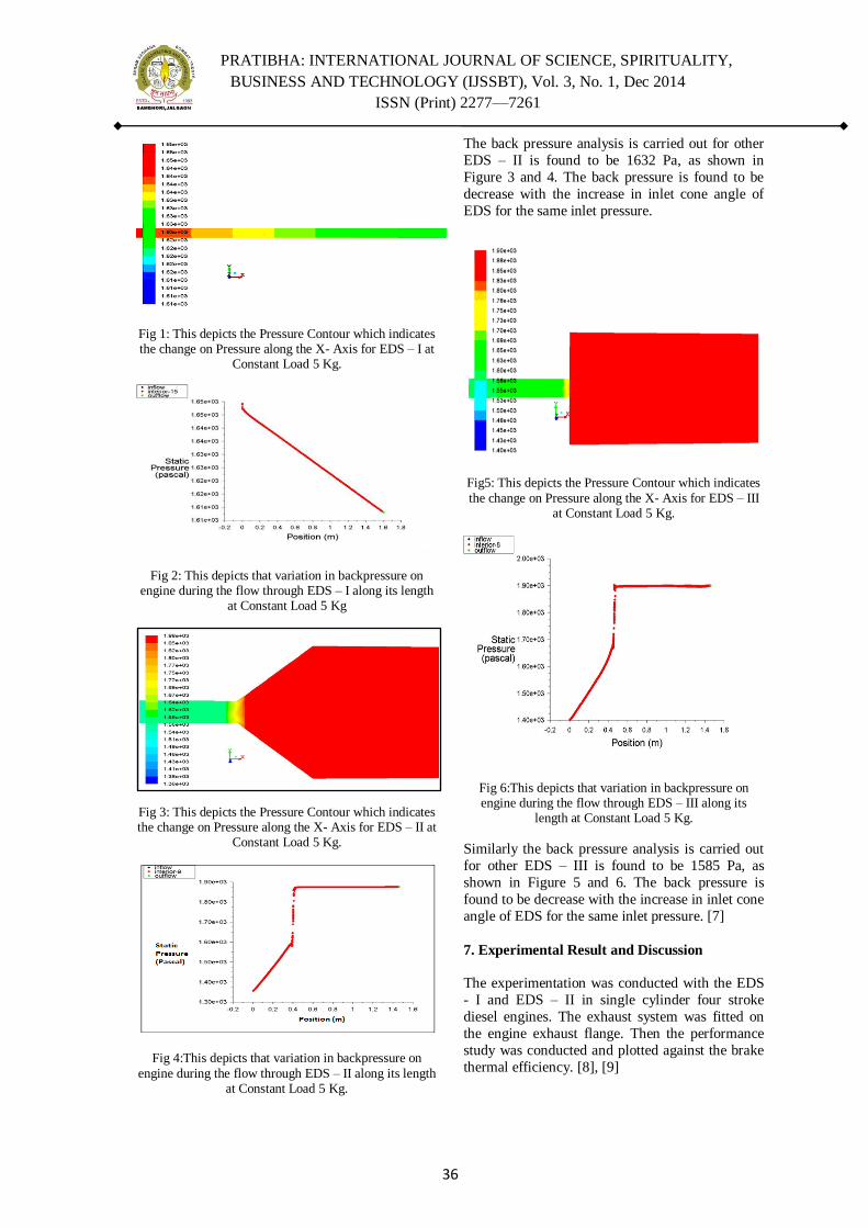
PRATIBHA: INTERNATIONAL JOURNAL OF SCIENCE, SPIRITUALITY,
BUSINESS AND TECHNOLOGY (IJSSBT), Vol. 3, No. 1, Dec 2014
ISSN (Print) 2277—7261
36
Fig 1: This depicts the Pressure Contour which indicates the change on Pressure along the X- Axis for EDS – I at
Constant Load 5 Kg.
Fig 2: This depicts that variation in backpressure on engine during the flow through EDS – I along its length
at Constant Load 5 Kg
Fig 3: This depicts the Pressure Contour which indicates the change on Pressure along the X- Axis for EDS – II at
Constant Load 5 Kg.
Fig 4:This depicts that variation in backpressure on
engine during the flow through EDS – II along its length at Constant Load 5 Kg.
The back pressure analysis is carried out for other
EDS – II is found to be 1632 Pa, as shown in
Figure 3 and 4. The back pressure is found to be
decrease with the increase in inlet cone angle of
EDS for the same inlet pressure.
Fig5: This depicts the Pressure Contour which indicates
the change on Pressure along the X- Axis for EDS – III at Constant Load 5 Kg.
Fig 6:This depicts that variation in backpressure on engine during the flow through EDS – III along its
length at Constant Load 5 Kg.
Similarly the back pressure analysis is carried out
for other EDS – III is found to be 1585 Pa, as
shown in Figure 5 and 6. The back pressure is
found to be decrease with the increase in inlet cone
angle of EDS for the same inlet pressure. [7]
7. Experimental Result and Discussion
The experimentation was conducted with the EDS
- I and EDS – II in single cylinder four stroke
diesel engines. The exhaust system was fitted on
the engine exhaust flange. Then the performance
study was conducted and plotted against the brake
thermal efficiency. [8], [9]
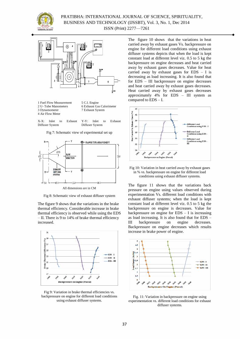
PRATIBHA: INTERNATIONAL JOURNAL OF SCIENCE, SPIRITUALITY,
BUSINESS AND TECHNOLOGY (IJSSBT), Vol. 3, No. 1, Dec 2014
ISSN (Print) 2277—7261
37
1 Fuel Flow Measurement 5 C.I. Engine
2 U- Tube Manometers 6 Exhaust Gas Calorimeter
3 Dynamometer 7 Exhaust System
4 Air Flow Meter
X-X: Inlet to Exhaust
Diffuser System
Y-Y: Inlet to Exhaust
Diffuser System
Fig 7: Schematic view of experimental set up
All dimensions are in CM
Fig 8: Schematic view of exhaust diffuser system
The figure 9 shows that the variations in the brake
thermal efficiency. Considerable increase in brake
thermal efficiency is observed while using the EDS
– II. There is 9 to 14% of brake thermal efficiency increased.
Fig 9: Variation in brake thermal efficiencies vs. backpressure on engine for different load conditions
using exhaust diffuser systems.
The figure 10 shows that the variations in heat
carried away by exhaust gases Vs. backpressure on
engine for different load conditions using exhaust
diffuser systems depicts that when the load is kept
constant load at different level viz. 0.5 to 5 kg the
backpressure on engine decreases and heat carried
away by exhaust gases decreases. Value for heat
carried away by exhaust gases for EDS – I is decreasing as load increasing. It is also found that
for EDS – III backpressure on engine decreases
and heat carried away by exhaust gases decreases.
Heat carried away by exhaust gases decreases
approximately 4% for EDS – III system as
compared to EDS – I.
Fig 10: Variation in heat carried away by exhaust gases
in % vs. backpressure on engine for different load conditions using exhaust diffuser systems.
The figure 11 shows that the variations back
pressure on engine using values observed during
experimentation Vs. different load conditions with exhaust diffuser systems; when the load is kept
constant load at different level viz. 0.5 to 5 kg the
backpressure on engine is decreases. Value for
backpressure on engine for EDS – I is increasing
as load increasing. It is also found that for EDS –
III backpressure on engine decreases.
Backpressure on engine decreases which results
increase in brake power of engine.
Fig. 11: Variation in backpressure on engine using experimentation vs. different load conditions for exhaust
diffuser systems.

PRATIBHA: INTERNATIONAL JOURNAL OF SCIENCE, SPIRITUALITY,
BUSINESS AND TECHNOLOGY (IJSSBT), Vol. 3, No. 1, Dec 2014
ISSN (Print) 2277—7261
38
Fig 12: Heat balance sheet for Exhaust Diffuser Systems
at constant load 5 Kg
It is observed from the Fig. 12, heat balance sheet
for different Exhaust diffuser systems at constant
load 5 kg; the heat balance sheet parameters that
are heat equivalent of brake power, heat carried by
the jacket cooling water, heat carried by exhaust
gases and heat unaccounted for. When the exhaust
diffuser systems are varies during the change of EDS - I to EDS – III the heat equivalent of brake
power increases and heat carried by exhaust gases
decreases. After testing it is observed that around
30 to 40%of fuel energy is wasted, this part is of
great concerned so as to maximize utilization of
exhaust energy. It is important to utilize the
exhaust energy through proper exhaust system
design.[11]
8.Conclusion
The following conclusions may be drawn from the
present study. The Exhaust system is successfully
designed. Through CFD analysis, the
backpressures of various Exhaust diffuser systems
are studied. The increase in inlet cone angle
increases the pressure of the flow which leads to
reduce the recirculation zones. Experimental setup
of the diffuser with different angles i.e.22.5, 45, 90
degree is design and fabricated. With the help of
C.I. engine test rig and suitable instrumentation
different parameters pressure, temperature, mass of
exhaust gases is determined. The exhaust gases from an optimal sized engine currently used, to
convert available Kinetic energy and enthalpy of
exhaust gases into the pressure energy for useful
after treatment of exhaust gases. This pressure is
being used and sent through diffuser which reduces
the back pressure. Installation of the EDS – III
increases the brake thermal efficiency and
decreases the backpressure.
This paper provides the experimental values
obtained during test for backpressure on engine
and the value obtained using CFD analysis for
backpressure on engine gives authenticity of data
for development of energy efficient exhaust
system. This was only made possible by the
approach adopted in this investigation.
Acknowledgments
Authors are thankful to the Godavari College of engineering, Jalgaon for providing laboratory
facility. The authors gratefully acknowledge the
support of the Ph.D. research Centre SSBTE‘S
College of engineering Jalgaon, without which
experimentationcould not have been done.
References
[1] J. B. Heywood; ―Internal Combustion Engine
Fundamentals‖; McGraw –Hill, ISBN 0-07-100499-8,
1988.
[2] R.G. Silver, J. C. Summers and W. B. Williamson,
―Design and Performance Evaluation of Automotive
Emission Control Catalysts‖, Evier Science Publishers B.
V. Amsterdam, 1991.
[3] Desmond E Winter Bone & Richard J Pearson, ―Theory
of Engine Manifold Design", Professional Engineering
Publishing, 2000.
[4] G.Venkatesh, ―Power Production Technique Using
Exhaust Gas From Present Automobiles via Convergent-
Divergent Nozzle‖, 0-7803-9794-0/06 IEEE, 2006.
[5] John D. Anderson, Jr., ―Computational Fluid Dynamics -
The Basic with Applications‖, McGraw - Hill
International Editions, 1995.
[6] MedaLakshmikantha& Mathias Keck, ―Optimization of
Exhaust Systems‖, SAE Paper No. 2002-01-0059, 2002.
[7] Atul A. Patil, Dr. L. G. Navale, Dr. V. S. Patil,
―Simulative Analysis of Single Cylinder Four Stroke C.I.
Engine Exhaust System‖, Pratibha International Journal of
science, Spirituality, Business and Technology (IJSSBT),
Vol. 3, ISSN (print) 2277-7261, November 2013, pp 79-
84.
[8] D.S. Deshmukh, J.P. Modak and K.M. Nayak,
"Experimental Analysis of Backpressure Phenomenon
Consideration for C.I. Engine Performance Improvement"
SAE Paper No. 2010-01-1575, International Powertrains,
Fuels & Lubricants Meeting, Rio De Janeiro, Brazil, on
dated- 5 May 2010.
[9] A.A. Patil, D.S. Deshmukh, L.G. Navale and V.S. Patil,
―Experimental Investigation of a C.I. Engine Operating
Parameters For Energy Efficient Exhaust System
Development" International Journal of Innovations In
Mechanical & Automobile Engineering (IJIMAE), ISSN
2249-2968 (Print), Sept.2011, Issue – I, Vol. -II, Pp. 60-
64
[10] Atul A. Patil, L. G. Navale, V. S. Patil, ―Experimental
Investigation and Analysis of Single Cylinder Four Stroke
C. I. Engine Exhaust System‖,
International Journal of Energy and Power (IJEP) Volume
3 Issue 1, February 2014, pp. 1-6.
[11] Atul A. Patil, L. G. Navale and V. S. Patil, ―Design,
Analysis of Flow Characteristics of Exhaust System and
Effect of Back Pressure on Engine Performance‖,
International Journal of Engineering, Business and
Enterprise Applications (IJEBEA) IJEBEA 14-165, ISSN
(Print): 2279-0020, ISSN (Online): 2279-0039, Volume 1,
Issue 7, February-2014, pp. 99-103.

PRATIBHA: INTERNATIONAL JOURNAL OF SCIENCE, SPIRITUALITY,
BUSINESS AND TECHNOLOGY (IJSSBT), Vol. 3, No. 1, Dec 2014
ISSN (Print) 2277—7261
39
IMPROVING EFFICIENCY OF SOLAR WATER HEATER
USING PHASE CHANGE MATERIALS
Mr. M.V. Kulkarni1,
Dr. D. S Deshmukh2,
1Asst. Professor, Department of Mechanical Engineering,
SSBT'S COLLEGE OF ENGINEERING AND TECHNOLOGY,
BAMBHORI, JALGAON - 425 001 (MS)
2H.O.D. Department of Mechanical Engineering,
SSBT's COLLEGE OF ENGINEERING AND TECHNOLOGY,
BAMBHORI, JALGAON - 425 001 (MS)
Abstract: The present work has been
undertaken to study the feasibility of storing
solar energy using Phase Change Materials
(PCMs) and utilizing this energy to heat water
for domestic purposes during nighttime. This
ensures that hot water is available throughout
the day. The system consists of two
simultaneously functioning heat-absorbing
units. One of them is a solar water heater and
the other a heat storage unit consisting of PCM
(paraffin). The water heater functions normally
and supplies hot water during the day. The
storage unit stores the heat in PCMs during the
day supplies hot water during the night. The
stainless steel water tank has a capacity of
about 30 litres, with an internal diameter of 28
cm and a height of 48 cm, it houses the 9 kg
PCM inside the square tank having length 40
cm & width 28cm and allows for heat transfer
between the surface and the water. Experiment
results show with using PCM cooling rate
during the night decrease & efficiency and heat
storage capacity increases.
Abbreviations
SWH Solar Water Heater PCM Phase Change Material
FPC Flat Plate Collector
MS Mild Steel
PVC Poly Vinyl Chloride
ICS Integrated Collector Storage
SHS Sensible Heat Storage
TES Thermal Energy Storage
LHTES Latent Heat Thermal Energy Storage
HTF Heat Transfer Fluid
1 Introduction
1.1 Phase Change Material
These materials can store energy by the
melting at a constant temperature. No material has
all the optimal characteristics for a PCM, and the
selection of a PCM for a given application requires
careful consideration of the properties of various
substances. Over 20,000 com-pounds and/or
mixtures have been considered in PCM, including single component systems, congruent mixtures,
eutectics and peritectics [3]. The isothermal
operating characteristics (i.e. charging/discharging
heat at a nearly constant temperature) during the
solidification and melting processes, which is
desirable for efficient operation of thermal systems
[9].
The value of the latent heat is very
important, because the higher latent heat results
higher storable heat quantity. According these
aspects we can choose from several materials. We
have to mind the chemical properties, the thermal expansion and the aspects of safety. PCMs in the
50 to 1000 temperature range have been proposed
to water heating and o -peak electrical heater
applications.
Wax is the most commonly used
commercial organic heat storage PCM [10].
Paraffin waxes are cheap and have moderate
thermal energy storage density but low thermal
conductivity and, hence, require large surface area
[10]. In our current project we are considering the
same PCM.
2 Experimental Investigations
2.1 Experiment setup
Photographs of the experimental setup
shown with the solar collector connected to the
water tank are shown in Figures 1. The setup
consists of a cylindrical water tank which holds the
PCM inside inner square tank, solar flat plate
collector. The stainless steel water tank has a
capacity of about 30 litres, capable of supplying
water for a family of four members. With an internal diameter of 28 cm and a height of 48 cm,
it houses the PCM inside the square tank having
length 40 cm & width 28cm and allows for heat
transfer between the surface and the water. The

PRATIBHA: INTERNATIONAL JOURNAL OF SCIENCE, SPIRITUALITY,
BUSINESS AND TECHNOLOGY (IJSSBT), Vol. 3, No. 1, Dec 2014
ISSN (Print) 2277—7261
40
tank is insulated with 5 cm of Rock wool and is
provided with an aluminium cladding. The PCM
storage tank contains 9 kg of paraffin wax. RTDs
are provided at inlet & outlet.
Fig 1: Experimental setup
2.2 Experiment trial
During the charging process the water is
circulated through the tank and the solar collector
unit continuously. The water absorbs solar energy
sensibly, and exchanges this heat with the PCM in
the PCM storage tank, which is initially at room
temperature. The PCM slowly gets heated,
sensibly at first, until it reaches its melting point
temperature. As the charging proceeds, energy
storage as Latent heat is achieved as the Paraffin wax melts at constant temperature (62±2°C). After
complete melting is achieved, further heat addition
from the water causes the PCM to superheat,
thereby again storing heat sensibly. The charging
process continues till the PCM and the water attain
thermal equilibrium. Temperatures of the PCM and
water at the outlet are recorded at intervals of 3
hours. The PCM is charged through the day,
whenever hot water is not demanded by the user.
The discharging process used is termed as
batch wise process. In this method, a certain quantity of hot water is withdrawn from the water
tank and readings are taken. This is then repeated
for intervals of 3 hours, in which time transfer of
energy from the PCM would have occurred. This
procedure is continued till PCM reaches a
temperature of 560C.
First of all we have taken the trial on the Solar
Water Heater without using phase change material
(WAX).
Phase 1
We calculated the cooling rate of the water in the
water tank after heating the water for 6hrs sunlight.
The analysis is shown in the Table 2.1
Table 1: Cooling rates of Water in General SWH
Time elapsed (hrs) Temperature0C
0 75
3 70
6 66
9 62
12 59
15 56
18 54
21 52
Phase 2
In this phase we were calculating the efficiency of
Solar Water Heater. The parameter s for
calculating the efficiency of Solar water heater as
shown in Table 2.2.
Table 2: Efficiency Parameters
We know the standard formula for efficiency
calculation
Efficiency, ɳ =
= Qout /Qin
Now, to calculate output Heat energy Qout = Heat
energy absorbed by water
ρ ×V ×Cpw ×( Tf - Ti )
Parameters Symbol Value
Volume of water V 20liter
Initial Temperature of water
Ti 360C
Heat radiated in day Pin 1170 Watts
Time elapsed t 6hrs
Final Temperature of
water Tf 750C

PRATIBHA: INTERNATIONAL JOURNAL OF SCIENCE, SPIRITUALITY,
BUSINESS AND TECHNOLOGY (IJSSBT), Vol. 3, No. 1, Dec 2014
ISSN (Print) 2277—7261
41
let‘s calculate heat supplied by solar radiation
Average heat radiated in a day, Pin = 1170 W/m2
Hence, Qin = Pin ×area of panel× Δ t
The absorption of radiated heat is only 96%
effective. So, effective heat radiated on panel
Q in,effective = 0.96 Qin
Now, calculating efficiency of general solar water
heater without using phase change material
ɳ = Qout / Q in,effective
Now, calculating cooling rate and the efficiency of
the solar water heater by adding PCM (Wax).
We added 9kg PCM (wax) in PCM tank as 100
liter water requires 36kg of PCM. Phase 1
We calculated the cooling rate of water in the
water tank by adding PCM and heating water for 6
Hrs.
The analysis is shown in the Table 2.3.
Table 3: Cooling rates of Water in SWH with PCM
Phase 2
Then calculate the efficiency of solar water heater.
The parameters for calculating the efficiency of
solar water heater are shown in Table 2.4.
Table 4: Efficiency Parameters
Parameters Symbol Value
Volume of water V 20liter
Initial Temperature of
water Ti 400C
Heat radiated in day Pin 1170 Watts
Time elapsed t 6hrs
Final Temperature of
water Tf 680C
Now, specification of PCM,
Initial temperature of PCM = 360C
Temperature of fusion = 600C
Final temperature of PCM = 650C
Specific heat of solid PCM = 2.5
Specific heat of molten PCM =215
Heat of Fusion=2.13
Now, calculating efficiency of solar water heater,
Efficiency, ɳ = = Qout / Qin
Now, calculating heat accumulated in the solar
collector, which is sum of energy gained by water
and same by PCM.
Energy gained by water =ρ×V×Cpw × ( Tf - Ti )
Energy gained by water = Energy accumulated by
solid PCM + Heat of fusion + Energy accumulated
by molten PCM
Qout = Energy gained by water + Energy gained by
PCM
ɳ = Qout / Qin;eff
3 Results and Discussion
The temperature distributions of water and the
PCM in the water tank for different time intervals
are recorded during charging and discharging
processes. The cumulative heat stored and system
efficiency of process is studied in detail during the
discharging process.
Time elapsed (hrs) Temperature of water0C
0 68
3 65
6 63
9 61
12 60
15 59
18 57
21 56
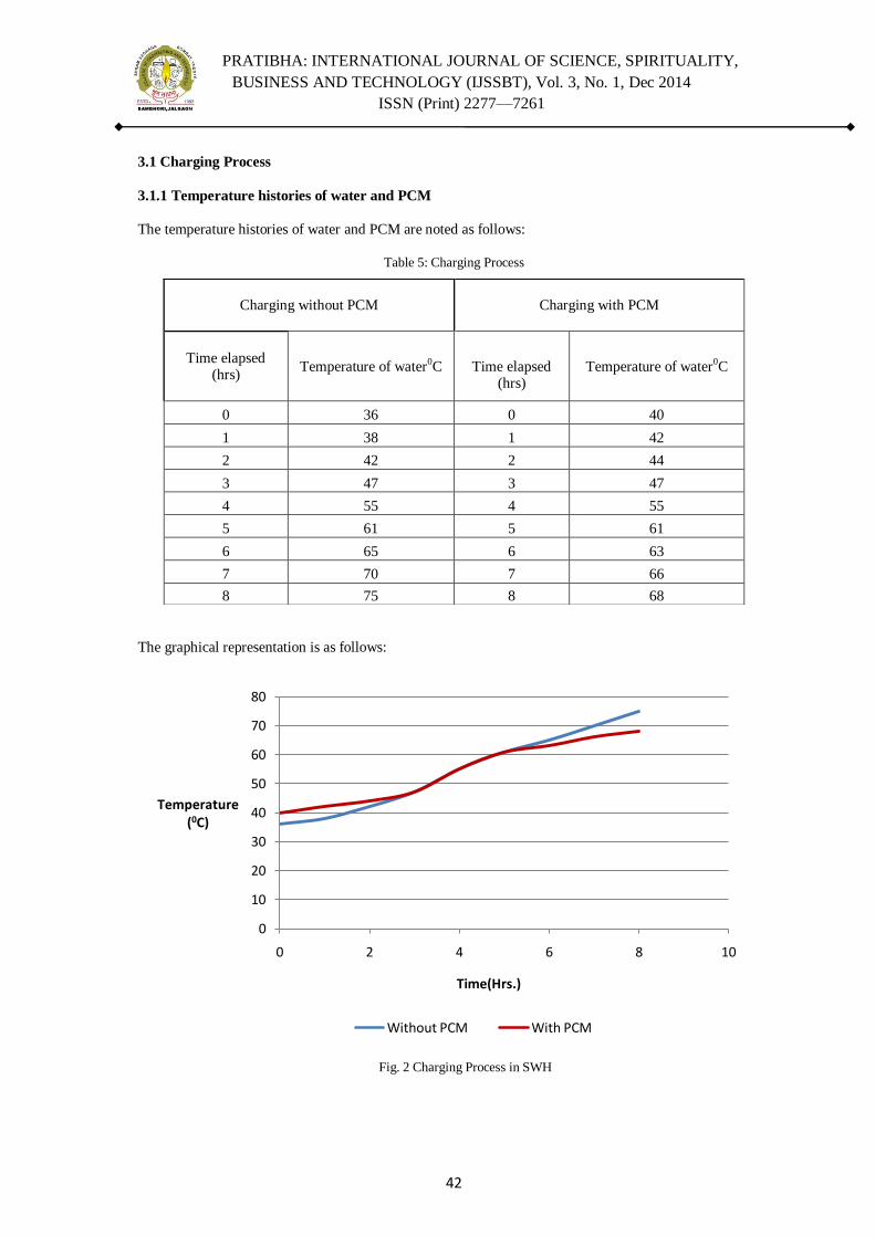
PRATIBHA: INTERNATIONAL JOURNAL OF SCIENCE, SPIRITUALITY,
BUSINESS AND TECHNOLOGY (IJSSBT), Vol. 3, No. 1, Dec 2014
ISSN (Print) 2277—7261
42
3.1 Charging Process
3.1.1 Temperature histories of water and PCM
The temperature histories of water and PCM are noted as follows:
Table 5: Charging Process
The graphical representation is as follows:
0
10
20
30
40
50
60
70
80
0 2 4 6 8 10
Temperature(0C)
Time(Hrs.)
Fig. 2 Charging Process in SWH
Without PCM With PCM
Charging without PCM
Charging with PCM
Time elapsed (hrs)
Temperature of water0C
Time elapsed (hrs)
Temperature of water0C
0 36 0 40
1 38 1 42
2 42 2 44
3 47 3 47
4 55 4 55
5 61 5 61
6 65 6 63
7 70 7 66
8 75 8 68
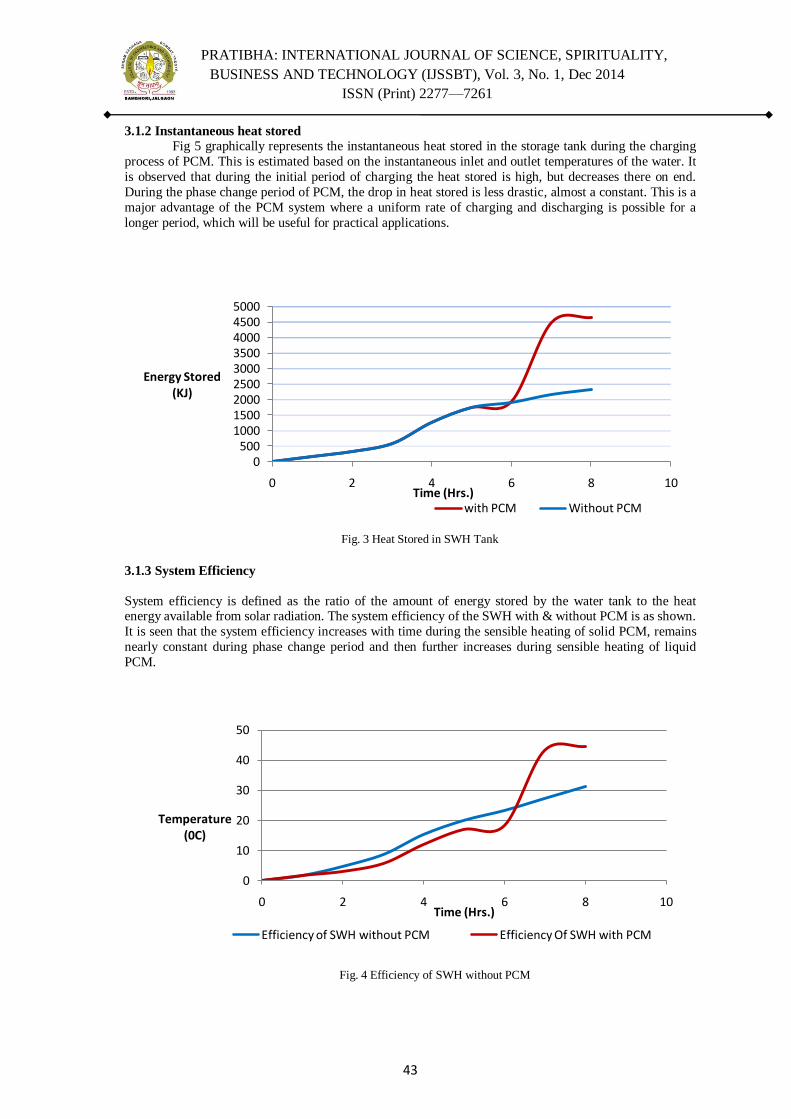
PRATIBHA: INTERNATIONAL JOURNAL OF SCIENCE, SPIRITUALITY,
BUSINESS AND TECHNOLOGY (IJSSBT), Vol. 3, No. 1, Dec 2014
ISSN (Print) 2277—7261
43
3.1.2 Instantaneous heat stored
Fig 5 graphically represents the instantaneous heat stored in the storage tank during the charging
process of PCM. This is estimated based on the instantaneous inlet and outlet temperatures of the water. It
is observed that during the initial period of charging the heat stored is high, but decreases there on end.
During the phase change period of PCM, the drop in heat stored is less drastic, almost a constant. This is a
major advantage of the PCM system where a uniform rate of charging and discharging is possible for a
longer period, which will be useful for practical applications.
3.1.3 System Efficiency
System efficiency is defined as the ratio of the amount of energy stored by the water tank to the heat energy available from solar radiation. The system efficiency of the SWH with & without PCM is as shown.
It is seen that the system efficiency increases with time during the sensible heating of solid PCM, remains
nearly constant during phase change period and then further increases during sensible heating of liquid
PCM.
0500
100015002000250030003500400045005000
0 2 4 6 8 10
Energy Stored(KJ)
Time (Hrs.)
Fig. 3 Heat Stored in SWH Tank
with PCM Without PCM
0
10
20
30
40
50
0 2 4 6 8 10
Temperature(0C)
Time (Hrs.)
Fig. 4 Efficiency of SWH without PCM
Efficiency of SWH without PCM Efficiency Of SWH with PCM
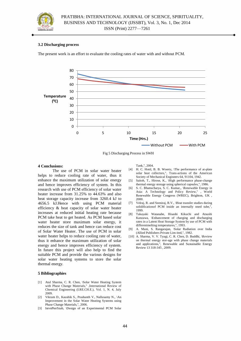
PRATIBHA: INTERNATIONAL JOURNAL OF SCIENCE, SPIRITUALITY,
BUSINESS AND TECHNOLOGY (IJSSBT), Vol. 3, No. 1, Dec 2014
ISSN (Print) 2277—7261
44
3.2 Discharging process
The present work is an effort to evaluate the cooling rates of water with and without PCM.
4 Conclusions:
The use of PCM in solar water heater
helps to reduce cooling rate of water, thus it
enhance the maximum utilization of solar energy
and hence improves efficiency of system. In this
research with use of PCM efficiency of solar water heater increase from 31.25% to 44.63% and also
heat storage capacity increase from 3260.4 kJ to
4656.5 kJ.Hence with using PCM material
efficiency & heat capacity of solar water heater
increases at reduced initial heating rate because
PCM take heat to get heated. As PCM based solar
water heater store maximum solar energy, it
reduces the size of tank and hence can reduce cost
of Solar Water Heater. The use of PCM in solar
water heater helps to reduce cooling rate of water,
thus it enhance the maximum utilization of solar
energy and hence improves efficiency of system. In future this project will also help to find the
suitable PCM and provide the various designs for
solar water heating systems to store the solar
thermal energy.
5 Bibliographies [1] Atul Sharma, C. R. Chen, \Solar Water Heating System
with Phase Change Materials," ,International Review of
Chemical Engineering (I.RE.CH.E.), Vol. 1, N. 4, July
2009.
[2] Vikram D., Kaushik S., Prashanth V., Nallusamy N., \An
Improvement in the Solar Water Heating Systems using
Phase Change Materials,", 2006.
[3] IstvnPterSzab, \Design of an Experimental PCM Solar
Tank,", 2004.
[4] H. C. Hottl, B. B. Woertz, \The performance of at-plate
solar heat collectors,", Trans-actions of the American
Society of Mechanical Engineers 64, 91104, 1942.
[5] Saitoh, T., Hirose, K., \High performance phase-change
thermal energy storage using spherical capsules,", 1986.
[6] S. C. Bhattacharya, S. C. Kumar,, \Renewable Energy in
Asia: A Technology and Policy Review," , World
Renewable Energy Congress (WREC), Brighton, UK ,
2000.
[7] Velraj, R. and Seeniraj, R.V., \Heat transfer studies during
solidificationof PCM inside an internally nned tube,",
1999.
[8] Takayaki Watanabe, Hisashi Kikuchi and Atsushi
Kanzawa, \Enhancement of charging and discharging
rates in a Latent Heat Storage System by use of PCM with
differentmelting temperatures,", 1993.
[9] A. Mani, S. Rangarajan, \Solar Radiation over India
(Allied Publishers Private Lim-ited,", 1982.
[10] A. Sharma, V. V. Tyagi, C. R. Chen, D. Buddhi, \Review
on thermal energy stor-age with phase change materials
and applications,", Renewable and Sustainable Energy
Review 13 318-345 , 2009.
0
10
20
30
40
50
60
70
80
0 5 10 15 20 25
Temperature(0C)
Time (Hrs.)
Fig 5 Discharging Process in SWH
Without PCM With PCM
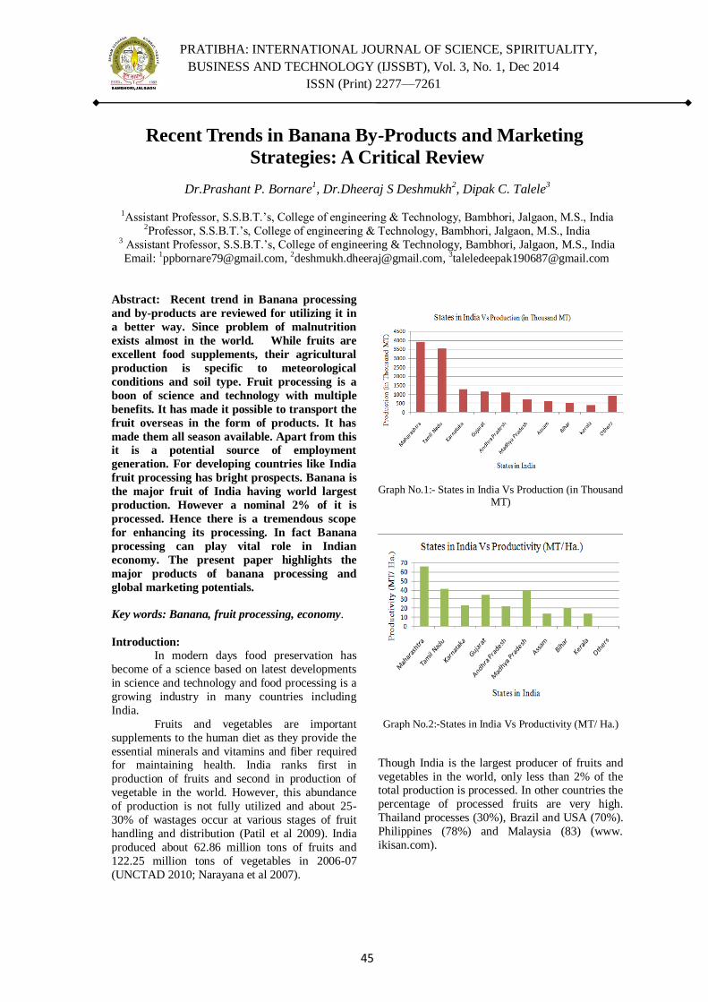
PRATIBHA: INTERNATIONAL JOURNAL OF SCIENCE, SPIRITUALITY,
BUSINESS AND TECHNOLOGY (IJSSBT), Vol. 3, No. 1, Dec 2014
ISSN (Print) 2277—7261
45
Recent Trends in Banana By-Products and Marketing
Strategies: A Critical Review
Dr.Prashant P. Bornare1, Dr.Dheeraj S Deshmukh
2, Dipak C. Talele
3
1Assistant Professor, S.S.B.T.‘s, College of engineering & Technology, Bambhori, Jalgaon, M.S., India
2Professor, S.S.B.T.‘s, College of engineering & Technology, Bambhori, Jalgaon, M.S., India 3 Assistant Professor, S.S.B.T.‘s, College of engineering & Technology, Bambhori, Jalgaon, M.S., India
Email: [email protected], [email protected], [email protected]
Abstract: Recent trend in Banana processing
and by-products are reviewed for utilizing it in
a better way. Since problem of malnutrition
exists almost in the world. While fruits are
excellent food supplements, their agricultural
production is specific to meteorological
conditions and soil type. Fruit processing is a
boon of science and technology with multiple
benefits. It has made it possible to transport the
fruit overseas in the form of products. It has
made them all season available. Apart from this
it is a potential source of employment
generation. For developing countries like India
fruit processing has bright prospects. Banana is
the major fruit of India having world largest
production. However a nominal 2% of it is
processed. Hence there is a tremendous scope
for enhancing its processing. In fact Banana
processing can play vital role in Indian
economy. The present paper highlights the
major products of banana processing and
global marketing potentials.
Key words: Banana, fruit processing, economy.
Introduction:
In modern days food preservation has
become of a science based on latest developments
in science and technology and food processing is a
growing industry in many countries including
India.
Fruits and vegetables are important
supplements to the human diet as they provide the
essential minerals and vitamins and fiber required for maintaining health. India ranks first in
production of fruits and second in production of
vegetable in the world. However, this abundance
of production is not fully utilized and about 25-
30% of wastages occur at various stages of fruit
handling and distribution (Patil et al 2009). India
produced about 62.86 million tons of fruits and
122.25 million tons of vegetables in 2006-07
(UNCTAD 2010; Narayana et al 2007).
Graph No.1:- States in India Vs Production (in Thousand
MT)
Graph No.2:-States in India Vs Productivity (MT/ Ha.)
Though India is the largest producer of fruits and
vegetables in the world, only less than 2% of the total production is processed. In other countries the
percentage of processed fruits are very high.
Thailand processes (30%), Brazil and USA (70%).
Philippines (78%) and Malaysia (83) (www.
ikisan.com).
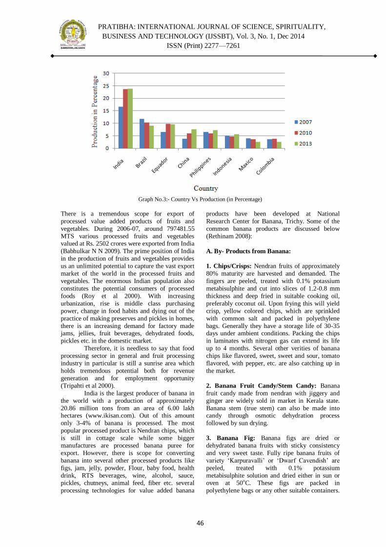
PRATIBHA: INTERNATIONAL JOURNAL OF SCIENCE, SPIRITUALITY,
BUSINESS AND TECHNOLOGY (IJSSBT), Vol. 3, No. 1, Dec 2014
ISSN (Print) 2277—7261
46
Graph No.3:- Country Vs Production (in Percentage)
There is a tremendous scope for export of
processed value added products of fruits and
vegetables. During 2006-07, around 797481.55
MTS various processed fruits and vegetables valued at Rs. 2502 crores were exported from India
(Babhulkar N N 2009). The prime position of India
in the production of fruits and vegetables provides
us an unlimited potential to capture the vast export
market of the world in the processed fruits and
vegetables. The enormous Indian population also
constitutes the potential consumers of processed
foods (Roy et al 2000). With increasing
urbanization, rise is middle class purchasing
power, change in food habits and dying out of the
practice of making preserves and pickles in homes,
there is an increasing demand for factory made jams, jellies, fruit beverages, dehydrated foods,
pickles etc. in the domestic market.
Therefore, it is needless to say that food
processing sector in general and fruit processing
industry in particular is still a sunrise area which
holds tremendous potential both for revenue
generation and for employment opportunity
(Tripahti et al 2000).
India is the largest producer of banana in
the world with a production of approximately
20.86 million tons from an area of 6.00 lakh hectares (www.ikisan.com). Out of this amount
only 3-4% of banana is processed. The most
popular processed product is Nendran chips, which
is still in cottage scale while some bigger
manufactures are processed banana puree for
export. However, there is scope for converting
banana into several other processed products like
figs, jam, jelly, powder, Flour, baby food, health
drink, RTS beverages, wine, alcohol, sauce,
pickles, chutneys, animal feed, fiber etc. several
processing technologies for value added banana
products have been developed at National
Research Center for Banana, Trichy. Some of the
common banana products are discussed below
(Rethinam 2008):
A. By- Products from Banana:
1. Chips/Crisps: Nendran fruits of approximately
80% maturity are harvested and demanded. The
fingers are peeled, treated with 0.1% potassium
metabisulphite and cut into slices of 1.2-0.8 mm
thickness and deep fried in suitable cooking oil,
preferably coconut oil. Upon frying this will yield
crisp, yellow colored chips, which are sprinkled
with common salt and packed in polyethylene
bags. Generally they have a storage life of 30-35 days under ambient conditions. Packing the chips
in laminates with nitrogen gas can extend its life
up to 4 months. Several other verities of banana
chips like flavored, sweet, sweet and sour, tomato
flavored, with pepper, etc. are also catching up in
the market.
2. Banana Fruit Candy/Stem Candy: Banana
fruit candy made from nendran with jiggery and
ginger are widely sold in market in Kerala state.
Banana stem (true stem) can also be made into candy through osmotic dehydration process
followed by sun drying.
3. Banana Fig: Banana figs are dried or
dehydrated banana fruits with sticky consistency
and very sweet taste. Fully ripe banana fruits of
variety ‗Karpuravalli‘ or ‗Dwarf Cavendish‘ are
peeled, treated with 0.1% potassium
metabisulphite solution and dried either in sun or
oven at 50oC. These figs are packed in
polyethylene bags or any other suitable containers.

PRATIBHA: INTERNATIONAL JOURNAL OF SCIENCE, SPIRITUALITY,
BUSINESS AND TECHNOLOGY (IJSSBT), Vol. 3, No. 1, Dec 2014
ISSN (Print) 2277—7261
47
They have a shelf life of about 3-4 months under
ambient conditions.
4. Banana Flour: Banana flour is prepared from
mature green bananas, which have a high starch
content. It can be used as nutritious adjuvant in
several food preparations like bread, cakes,
biscuits, health drink and baby food formulations. It can also be blended with other cereal flours for
making chapaties and roties. It has some medicinal
property to cure ulcers. Under cool and dry
conditions it can be stored up to one year without
any adverse change in their composition.
5. Banana Powder: Banana powder is prepared
from fully ripe banana fruits either through drum
drying or spray drying process. The moisture
content of final product should be around 2-4%.
This product has got high market value as it is
extensively used in confectionary industry, ice cream preparations and baby food making. When
suitably packed it will have a shelf life of more
than 6 months.
6. Banana Juice: Since banana puree is very thick,
juice cannot be directly obtained from it.
Therefore, the puree is treated with pectolytic
enzyme and clear juice is obtained through
filtration or centrifugation. After pasteurization
and bottling it can have a shelf life of a minimum
of 6 months under ambient conditions.
7. Banana Fruit Bar: Banana Fruit Bar is
confectionary item prepared from ripe banana fruit
of any variety. It is made by homogenizing banana
pulp, sugar, citric acid and pectin in suitable
proportions and dehydrating the mass in ghee
coated ray at 70o C in an oven till sets into a sheet.
It is then cut into suitable size and packed in
polyethylene pouches.
8. Banana Biscuits: Banana biscuits are made by mixing 60% banana flour and 30% maida. The
dough is made using flour mixture and suitable
proportions of sugar, saturated fat, baking powder,
milk powder and essence. These biscuits are very
tasty and highly nutritious.
9. Banana Jam & Jelly: Banana jam is made by
cooking the fruit pulp with sugar along with pectin
and citric acid in right proportions till gives a good
set. Several varieties of banana are suitable for
making jam. This is product, which has good
commercial value and good market. Banana jelly is a semi solid product
prepared by boiling clear strained fruit extract free
from pulp after addition of required amount of
sugar, citric acid and pectin. A perfect jelly should
be transparent, attractive and sparkling in color
with strong flavor of fruit.
10. Banana Wine: Banana wine is produced by
fermenting the enzyme treated clear banana juice
with wine yeast viz . Saccharomyces cerevisae var.
ellipaoiswua. The fermentation is carried out for
about 3 weeks followed by filtration, clarification, and bottling. The pasteurized wine is stored in
bottles for aging. The alcohol content of banana
varies from 9-12%.
11. Health drinks and Baby food: A highly
nutritious and tasty health drink formulations and
baby food formula has been developed by NRCB
using banana flour/powder after supplementing
with suitable natural source of proteins ,minerals
,vitamins and fat . It has got a shelf life of about 6
months and suitable is for children and adults.
12. Banana Fiber: Banana fiber is extracted from
the pseoudostem, peduncles and dried petioles and
of banana plant . The banana fiber can be used for
manufacture special kind of papers, ropes, threads,
baskets, toys and several fancy items. The yarn
made form banana fiber is much in demand for
making textiles.
Conclusions:
It is quite obvious from the forgoing discussion
that there is a vast scope for developing by-products of banana. The post globalization world
economy gives more weightage on processing and
value addition. This industry can play a vital role
in the economic uplifting of the country specially
the agricultural section. In fact this is going to be
the second phase of green revolution. Thus, food
preservation and proper low cost consumption to
reduce malnutrition problem is possible through
banana fruit. and it‘s by-products.
References:
[1] Babhulkar N N (2009) Fruit production development,
Shetkari, 43, pp 98.
[2] Narayana C K and Mustaffa M M (2007) Value addition
in banana, in the Proceedings of National Conference on
Banana held during October 25 – 28, 2007 at
Tiruchirapalli, TN.
[3] Rethinam P (2008) Banana for food and nutritional
security, in the Proceedings of International Conference
on Banana held during October 24 – 26, 2007 at
Tiruchirapalli, TN.
[4] Patil K B and Rawale K P (2009) Pre and post harvest
management of banana for domestic and export market, in
the Proceedings of Second National Conference on
Production of Healthy Planting Material in Banana, held
during October 3 - 6, 2009 at Jalgaon MS.
[5] UNCTAD- United Nations Council of Trade and
Agriculture Development Secretarial Promulgation
available on Wikipedia.

PRATIBHA: INTERNATIONAL JOURNAL OF SCIENCE, SPIRITUALITY,
BUSINESS AND TECHNOLOGY (IJSSBT), Vol. 3, No. 1, Dec 2014
ISSN (Print) 2277—7261
48
[6] Tripathi S N and Anju B (2000) Storage system of fruits,
vegetables and their products, Indus Publishing Co, New
Delhi.
[7] Roy S K, Pal R K and Sen N (2000) Packaging
Technologies for fruits, vegetables and their products,
Indus Publishing Co, New Delhi
[8] Sherlekar S A (2006) Marketing Management, Himalaya
Publishing House, Mumbai.
[9] Singh H P (2008) Research and Development of banana
and plantain in India, in the Proceedings of International
Conference on Banana held during October 24 to 26 2008,
at Tiruchirapalli, TN.

PRATIBHA: INTERNATIONAL JOURNAL OF SCIENCE, SPIRITUALITY,
BUSINESS AND TECHNOLOGY (IJSSBT), Vol. 3, No. 1, Dec 2014
ISSN (Print) 2277—7261
49
EFFECTS OF GROUNDING SYSTEM ON POWER
QUALITY
Bhagat Singh Tomar, Dwarka Prasad, Apeksha Narendra Rajput
Research Scholar, Electrical Engg. Department,
Laxmi Devi Institute of Engg. & Technology, Alwar,(Rajasthan),India
Associate Professor, Electrical Engg. Department,
Laxmi Devi Institute OfEngg. & Technology, Alwar,(Rajasthan),India, Junior Engineer-I,RajasthanRajyaVidyutPrasarannigam Limited(RRVPNL), Alwar,(Rajasthan),India
[email protected], [email protected], [email protected]
Abstract—The purpose of this paper is to
present the importance and affects of grounding
and harmonics to the quality of power. The
power quality conditions significantly depends
on the every aspect in electrical system such as
voltage, current, frequency, power, power
factor and so on. As the result of this analysis,
the grounding conditions used in the data
center was found to have no signs of severity in
power quality conditions. However, there were
some issues of improper wiring and grounding
found in the systems. On the other hand, the
harmonic distortion in data center was
discussed in terms of the source of harmonics
effects of harmonic on the performance of data
center. In order to identify the cause of such
orders of harmonics in this system, the most
non linear load is identified. Therefore, some
recommendations and mitigations of the
harmonics were discussed.
IndexTerms— Grounding, Harmonics , Power
Quality, data center, Voltage Levels.
I.INTRODUCTION
Power quality issues can be very high-speed events
such as transients, harmonic, high frequency noise,
faulty wiring of grounding system, voltage swells
and sags and total power loss. In this analysis,
grounding and harmonics will be discussed in terms of power quality. Grounding may not be
complicated but when a lack of understanding
mixes with folklore and tradition, it may become
exceedingly complex. It has been reported that 80
to 90% of power quality problems are mostly
caused by improper wiring and grounding.
Grounding is defined as a conducting connection,
whether intentional or unintentional by which an
electric circuit or equipment is connected to the earth or to some conducting body relatively large
that serves in place of the earth. Grounding system
designs and operations are completely depends on
the applications in particular requirements. By
specializing the grounding techniques can evolve
the complexion of grounding system topic to meet
the perceived grounding requirements of electronic
equipment. The assessments include representation
of grounding systems with linear and nonlinear
parameters to produce a better representation of the
overall electrical system at abnormal operating conditions [1].
Another power quality issue is harmonic
[2]. Harmonic is defined as sinusoidal component
of a periodic waveform having a frequency that is
an integer multiple of having fundamental
frequency. It is also a mathematical model that
used to analyzed distorted waveforms and can be
generated by non linear electronic loads[3]. The
harmonic related losses reduce system efficiency,
cause apparatus overheating, and increase power
and air conditioning costs. The harmonic currents
can have a significant impact on electrical distribution systems and the facilities they feed.
II. BASIC ON HARMONICS
The basic harmonic theory which according to
Fourier theorem, periodic non-sinusoidal or
complex voltage (Figure 2) or current waveforms
can be represented by the sum of a series of
multiple frequency terms of varying magnitudes
and phases as shown in equation (1).
)]cos([)( 0 nn qtnaatf (1)
where: na is the magnitude of the nth harmonic
frequency
oa is the d.c. component
nq is the phase angle of the nth harmonic
frequency
is the fundamental frequency . n =1,2,3,…
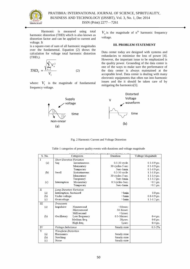
PRATIBHA: INTERNATIONAL JOURNAL OF SCIENCE, SPIRITUALITY,
BUSINESS AND TECHNOLOGY (IJSSBT), Vol. 3, No. 1, Dec 2014
ISSN (Print) 2277—7261
50
Harmonic is measured using total
harmonic distortion (THD) which is also known as
distortion factor and can be applied to current and
voltage. It
is a square-root of sum of all harmonic magnitudes
over the fundamental. Equation (2) shows the
calculation for voltage total harmonic distortion
(THDv).
1
2
2
V
V
THDn
n
V (2)
where: 1V is the magnitude of fundamental
frequency voltage.
nV is the magnitude of nth harmonic frequency
voltage.
III. PROBLEM STATEMENT
Data center today are designed with systems and
redundacies to minimize the loss of power [4].
However, the important issue to be emphasized is
the quality power. Grounding of the data center is
one of the ways to make sure the performance of
the data center is always maintained at the acceptable level. Data center is dealing with many
electronic equipments that often run into harmonic
issues and the it should be taken care of by
mitigating the harmonics[5].
Table 1 categories of power quality events with durations and voltage magnitude
Fig. 2 Harmonic Current and Voltage Distortion
(b)
V
time
Distorted Voltage waveform
Non-linear
current (a)
Supply voltage
time
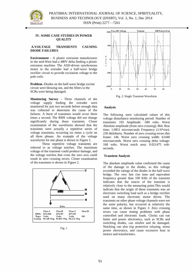
PRATIBHA: INTERNATIONAL JOURNAL OF SCIENCE, SPIRITUALITY,
BUSINESS AND TECHNOLOGY (IJSSBT), Vol. 3, No. 1, Dec 2014
ISSN (Print) 2277—7261
51
IV. SOME CASE STUDIES IN POWER
QUALITY
A.VOLTAGE TRANSIENTS CAUSING
DIODE FAILURES
Environment - A plastic extrusion manufacturer in the mid-West had a 480V delta feeding a plastic
extrusion machine. The ASD-driven synchronous
motor in the extruder had a half-wave bridge
rectifier circuit to provide excitation voltage to the
pole coils.
Problem -Diodes on the half-wave bridge exciter
circuit were blowing out, and the filters to the
SCRs were being damaged.
Monitoring Survey - Three channels of the
voltage supply feeding the extruder were monitored for just two seconds before enough data
was collected to determine the cause of the
failures. A burst of transients would occur three
times a second. The RMS voltage did not change
significantly during these transients. Closer
examination of the waveforms showed that the
transients were actually a repetitive series of
voltage transients, occurring six times a cycle on
all three phases. An example of the voltage
waveforms for one phase is shown in Figure 1.
These repetitive voltage transients are referred to as voltage notches. The maximum
voltage of the transient could produce damage, and
the voltage notches that cross the zero axis could
result in zero crossing errors. Closer examination
of the transients is shown in Figure 2.
Fig. 1
Fig. 2. Single Transient Waveform
Analysis
The following were calculated values of this
voltage disturbance monitoring period: Number of
transients: 192 Amplitude: -580 volts. Worst
Absolute amplitude (from zero crossing): 864. Rise
time: 1.0851 microseconds Frequency (1/4*rise):
230.4kilohertz. Number of zero crossing errors this frame: 146. Worst zero crossing width: 61440
microseconds. Worst zero crossing delta voltage:
168 volts. Worst notch area: 0.021475 volt-
seconds.
Transient Analysis
The absolute amplitude value confirmed the cause
of the damage to the diodes, as this voltage
exceeded the ratings of the diodes in the half-wave
bridge. The very fast rise time and equivalent frequency greater than 100 KHz of the transient
indicates that the source of the transient is
relatively close to the measuring point.This would
indicate that the origin of these transients was an
electronic switching load such as a bridge rectifier
used on many electronic motor drives. The
transients on other phase voltage channels were not
the same polarity, but occurred at relatively the
same time, as shown in Figure 3. Zero crossing
errors can cause timing problems with phase
controlled and electronic loads. Clocks can run
faster and power electronics, such as SCRs and switching diodes, can misfire and be damaged.
Notching can also trip protective relaying, stress
power electronics, and cause excessive heat in
motors and transformers.
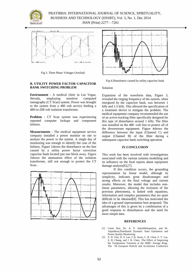
PRATIBHA: INTERNATIONAL JOURNAL OF SCIENCE, SPIRITUALITY,
BUSINESS AND TECHNOLOGY (IJSSBT), Vol. 3, No. 1, Dec 2014
ISSN (Print) 2277—7261
52
Fig 3. Three Phase Voltages Overlaid.
B. UTILITY POWER FACTOR CAPACITOR
BANK SWITCHING PROBLEM
Environment - A medical clinic in Las Vegas,
Nevada, employing sensitive computed
tomography (CT Scan) system. Power was brought
to the system from a 480 volt service feeding a
480-to-208 volt isolation transformer.
Problem - CT Scan system was experiencing
repeated computer lockups and component
failures.
Measurements - The medical equipment service
company installed a power monitor on site to
analyze the power to the system. A single day of
monitoring was enough to identify the case of the
failures. Figure 1shows the disturbance on the line
caused by a utility power factor correction
capacitor bank located just one block away. Figure
2shows the attenuation effect of the isolation transformer, still not enough to protect the CT
Scan .
Fig 4.Disturbance caused by utility capacitor bank
Solution
Expansion of the waveform data, Figure 3,
revealed the ringing frequency of the system, when energized by the capacitor bank, was between 1
kHz and 1.5 kHz. This allowed the specification of
a treatment device to mitigate the problem. The
medical equipment company recommended the use
of an active-tracking filter specifically designed for
this type of disturbance around 1 kHz. The filter
was installed on the 480 -volt line to protect all of
the downstream equipment. Figure 4shows the
difference between the input (Channel C) and
output (Channel B) of the filter during a
subsequent capacitor bank switching operation
IV.CONCLUSION
This work has been involved with investigations
associated with the various systems modelling and
its influence on the final reports about equipment
damage analysis[6],[7].
If this condition occurs, the grounding
representation by linear model, although its
simplicity, indicates great disadvantages and
strong effects on the final voltage and current
results. Moreover, the model that includes non-linear parameters, allowing the inclusion of the
previous phenomena, is linked with equations,
information and complex parameters that are quite
difficult to be obtained[8]. This has motivated the
idea of a ground representation here proposed. The
advantages of this is given by a combination of a
good response to disturbances and the need for
more simple data.
REFERENCES
[1] Curtis Roe, Dr. A. P. SakisMeliopoulos, and Dr.
AnjanBose,Distributed Dynamic State Estimation and
Power Quality Monitoring.
[2] Z. D. Tsai, D. S. Lee, C.K. Kuan, C. R. Chen, F. Y. Lin,
S. H. Chang, and J. R. Chen, .The Effect of Improving
the Temperature Variation at the SRRC Storage Ring.,
The 7th European Particle and Accelerator Conference

PRATIBHA: INTERNATIONAL JOURNAL OF SCIENCE, SPIRITUALITY,
BUSINESS AND TECHNOLOGY (IJSSBT), Vol. 3, No. 1, Dec 2014
ISSN (Print) 2277—7261
53
(EPAC), June 2000, Vienna, Austria. I. N. Gondim, J. C.
de Oliveira, C. E. Tavares, J. A. F. Barbosa Jr. and M. V.
B. Mendonça
[3] Grounding System Modelling and Its Impact on
Computational Refunding Analysis for Equipment
Damages.
[4] P. Ferracci, ― Power Quality‖, Schneider Electric Cahier
Technique no. 199, September 2000.
[5] D. Chapman, ―Costs of Poor Power Quality‖, Power
Quality Application Guide – Copper Development
Association, March 2001
[6] P. Ribeiro, B. Johnson, M. Crow, A. Arsoy, Y.
Liu,―Energy Storage Systems for Advanced Power
Applications‖, Proceedings of the IEEE, vol 89, no.12,
December 2001.
[7] D. Chapman, ―Costs of Poor Power Quality‖, Power
Quality Application Guide – Copper Development
Association, March 2001
[8] P. Ribeiro, B. Johnson, M. Crow, A. Arsoy, Y.
Liu,―Energy Storage Systems for Advanced Power
Applications‖, Proceedings of the IEEE, vol 89, no.12,
December 2001.
[9] Meier, Alexandra von (2006). Electric Power Systems: A
Conceptual Introduction. John Wiley & S
[10] Kusko, Alex; Marc Thompson (2007). Power Quality in
Electrical Systems. McGraw Hill.
[11] Mohamed Anwar Abou El-Ata‖Assessment of
uncertainties in substation groundingsystem using interval
mathematics‖,Ain Shams Engineering Journal (2012) 3,
27–31.

PRATIBHA: INTERNATIONAL JOURNAL OF SCIENCE, SPIRITUALITY,
BUSINESS AND TECHNOLOGY (IJSSBT), Vol. 3, No. 1, Dec 2014
ISSN (Print) 2277—7261
54
USE OF RGB COLORS AND CRYPTOGRAPHY FOR
COULD SECURITY
S. J. Patil Asst. Prof & Head,
Department of Information Technology.
SSBT‘s COET, Bambhori, Jalgaon, Maharashtra-425001
e-mail:[email protected]
N. P. Jagtap Asst. Prof. Department of Information Technology
SSBT‘s COET, Bambhori, Jalgaon, Maharashtra-425001
email:[email protected]
Shambhu Kumar Singh Department of Computer Sci. and Engineering
G. H. Raisoni Institute of Engineering and Management Jalgaon, Maharashtra-425001 [email protected]
AbstractCloud computing is a parallel and
distributed computing system consisting of a
collection of inter-connected and virtualized
computers that are dynamically provisioned
and presented as one or more unified
computing which is based on service level
agreement. In cloud computing data security
and privacy is one of the most challenges. So
secure delivery of data to and from the cloud is
however a serious issue that needs to be
addressed. This paper describes or fulfills the
current scenario of cloud computing by using
combination of both colors and Homomorphic
encryption technique simultaneously.
Keywords- Cloud Computing, Cloud Security,
Data Security, Homomorphic encryption.
1. INTRODUCTION
According to NIST (National Institute of standard and Technology) Cloud computing is a
model for enabling convenient, on-demand
network access to a shared pool of configurable
computing resources (e.g., networks, servers,
storage applications and services) that can be
rapidly provisioned and released with minimal
management effort or service provider interaction.
There are many problem related with cloud
computing traffic, security and resource
management. We can provide security in cloud by
many ways like on data, network and storage. Homomorphic encryption method provides more
security on data because provider is not involving
in key management. I have use proxy re-
encryption technique and colors technique that
prevents ciphertext from chosen cipher text attack.
This system is more secure than existing system.
By Cloud Computing we mean: The
Information Technology (IT) model for
computing, which is composed of all the IT
components (hardware, software, networking, and
services) that are necessary to enable development
and delivery of cloud services via the Internet or a
private network. This definition has no notion of security for data in the cloud computing even if it's
a very new. Cloud providers like: IBM, Google
and Amazon use the virtualization in their Cloud
platform, and in the same machine can coexist the
storage space and treatment virtualized which
belong to the concurrent enterprises.
In cloud computing, everything is
delivered as a Service (XaaS), from testing and
security, to collaboration and Meta modeling [8].
The cloud was rapidly becoming a conflagration of
buzzwords ―as a service‖. Today there are three
main service models, which are agreed on and defined in the NIST document [9].
1. Software as a Service {SaaS} - this simply
means delivering software over the Internet. It
is the most widely known model of cloud
computing. SaaS has been around since early
2001 when it was commonly referred to as the
Application Service Provider (ASP) Model
[8]. Software as a Service consists of software
running on the provider‘s cloud infrastructure,
delivered to (multiple) clients (on demand) via a thin client (e.g. browser) over the Internet.
Typical examples are Google Docs and
Salesforce.com CRM.

PRATIBHA: INTERNATIONAL JOURNAL OF SCIENCE, SPIRITUALITY,
BUSINESS AND TECHNOLOGY (IJSSBT), Vol. 3, No. 1, Dec 2014
ISSN (Print) 2277—7261
55
2. Platform as a Service {PaaS} - this gives a
client (developer) the flexibility to build
(develop, test and deploy) applications on the
provider‘s platform (API, storage and
infrastructure). PaaS stakeholders include the
PaaS hosted who provides the infrastructure
(servers etc), the PaaS provider who provides
the development tools and platform and the PaaS user [10]. Examples of PaaS are
Microsoft Azure and Google AppEngine.
3. Infrastructure as a Service {IaaS} - rather
than buy servers and build a datacenter from
ground up, and consequently having to worry
about what happens when the 1. Software as a
Service {SaaS} - this simply means delivering
software over the Internet. It is the most
widely known model of cloud computing.
SaaS has been around since early 2001 when it
was commonly referred to as the Application Service Provider (ASP) Model [8]. Software
as a Service consists of software running on
the provider‘s cloud infrastructure, delivered
to (multiple) clients (on demand) via a thin
client (e.g. browser) over the Internet. Typical
examples are Google Docs and
Salesforce.com CRM.
Depending on infrastructure ownership,
there are four deployment models of cloud
computing each with its merits and demerits. This is where the security issues start.
Fig 1 Architecture of cloud computing
1. The Public Cloud - this is the traditional view
of cloud computing in every day lingua. It is usually owned by a large organization (e.g.
Amazon‘s EC2, Google‘s AppEngine and
Microsoft‘s Azure). The owner-organization
makes its infrastructure available to the
general public via a multi-tenant model on a
self-service basis delivered over the Internet.
This is the most cost-effective model leading
to substantial savings for the user, albeit with
attendant privacy and security issues since the
physical location of the provider‘s
infrastructure usually traverses numerous
national boundaries.
2. The Private Cloud - refers to cloud
infrastructure in a single tenant environment. It defers from the traditional datacenter in its
predominant use of virtualization. It may be
managed by the tenant organization or by a
third party within or outside the tenant
premises. A private cloud costs more than the
public cloud, but it leads to more cost savings
when compared with a datacenter as
evidenced by Concur Technologies (est.
savings of $7million in 3 years from 2009)
[11]. The private cloud gives an organization
greater control over its data and resources. As
a result, the private cloud is more appealing to enterprises especially in mission and safety
critical organizations.
3. The Community Cloud - according to NIST,
the community cloud refers to a cloud
infrastructure shared by several organizations
within a specific community. It may be
managed by any one of the organizations or a
third party. A typical example is the Open
Cirrus Cloud Computing Tested, which is a
collection of Federated data centers across six sites spanning from North America to Asia
[12].
4. The Hybrid Cloud - comprises of a
combination of any two (or all) of the three
models discussed above. Standardization of
APIs has lead to easier distribution of
applications across different cloud models.
This enables newer models such as ―Surge
Computing‖ in which workload spikes from
the private cloud is offset to the public cloud.
2. HOMOMORPHIC ENCRYPTION
Homomorphic encryption alludes to encryption
where plain texts and cipher texts both are treated
with an equivalent algebraic function.
Homomorphic Encryption allows server to do
operation on encrypted data without knowing the
original plaintext. Homomorphic encryption allows
complex mathematical operations to be performed
on encrypted data without using the original data.
For plaintexts X1 and X2 and corresponding ciphertext Y1 and Y2, a Homomorphic encryption
scheme permits the computation of X1 Θ X2 from
Y1 and Y2 without using P1 Θ P2.The
cryptosystem is multiplicative or additive
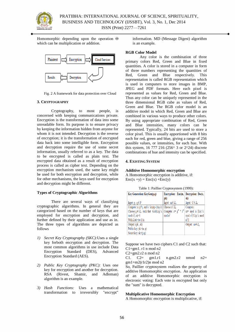
PRATIBHA: INTERNATIONAL JOURNAL OF SCIENCE, SPIRITUALITY,
BUSINESS AND TECHNOLOGY (IJSSBT), Vol. 3, No. 1, Dec 2014
ISSN (Print) 2277—7261
56
Homomorphic depending upon the operation Θ
which can be multiplication or addition.
Fig. 2 A framework for data protection over Cloud
3. CRYPTOGRAPHY
Cryptography, to most people, is
concerned with keeping communications private. Encryption is the transformation of data into some
unreadable form. Its purpose is to ensure privacy
by keeping the information hidden from anyone for
whom it is not intended. Decryption is the reverse
of encryption; it is the transformation of encrypted
data back into some intelligible form. Encryption
and decryption require the use of some secret
information, usually referred to as a key. The data
to be encrypted is called as plain text. The
encrypted data obtained as a result of encryption
process is called as cipher text. Depending on the encryption mechanism used, the same key might
be used for both encryption and decryption, while
for other mechanisms, the keys used for encryption
and decryption might be different.
Types of Cryptographic Algorithms
There are several ways of classifying
cryptographic algorithms. In general they are
categorized based on the number of keys that are
employed for encryption and decryption, and
further defined by their application and use as in. The three types of algorithms are depicted as
follows
1) Secret Key Cryptography (SKC):Uses a single
key forboth encryption and decryption. The
most common algorithms in use include Data
Encryption Standard (DES), Advanced
Encryption Standard (AES).
2) Public Key Cryptography (PKC): Uses one
key for encryption and another for decryption. RSA (Rivest, Shamir, and Adleman)
algorithm is an example.
3) Hash Functions: Uses a mathematical
transformation to irreversibly "encrypt"
information. MD (Message Digest) algorithm
is an example.
RGB Color Model
Any color is the combination of three
primary colors Red, Green and Blue in fixed
quantities. A color is stored in a computer in form
of three numbers representing the quantities of Red, Green and Blue respectively. This
representation is called RGB representation which
is used in computers to store images in BMP,
JPEG and PDF formats. Here each pixel is
represented as values for Red, Green and Blue.
Thus any color can be uniquely represented in the
three dimensional RGB cube as values of Red,
Green and Blue. The RGB color model is an
additive model in which Red, Green and Blue are
combined in various ways to produce other colors.
By using appropriate combination of Red, Green
and Blue intensities, many colors can be represented. Typically, 24 bits are used to store a
color pixel. This is usually apportioned with 8 bits
each for red, green and blue, giving a range of 256
possible values, or intensities, for each hue. With
this system, 16 777 216 (256^ 3 or 2^24) discrete
combinations of hue and intensity can be specified.
4. EXISTING SYSTEM
Additive Homomorphic encryption
A Homomorphic encryption is additive, if: Enc(x +y) = Enc(x) +Enc(y)
Table 1: Paillier Cryptosystem (1999):
Suppose we have two ciphers C1 and C2 such that:
C1=gm1. r1 n mod n2
C2=gm2.r2 n mod n2
C1. C2= gm1.r1 n.gm2.r2 nmod n2=
gm1+m2(r1r2)n mod n2 So, Paillier cryptosystem realizes the property of
additive Homomorphic encryption. An application
of an additive Homomorphic encryption is
electronic voting: Each vote is encrypted but only
the "sum" is decrypted.
Multiplicative Homomorphic Encryption
A Homomorphic encryption is multiplicative, if:

PRATIBHA: INTERNATIONAL JOURNAL OF SCIENCE, SPIRITUALITY,
BUSINESS AND TECHNOLOGY (IJSSBT), Vol. 3, No. 1, Dec 2014
ISSN (Print) 2277—7261
57
Enc(x *y) = Enc(x) *Enc(y)
Table 2: RSA Cryptosystem (1978)
Suppose we have two ciphers C1 and C2 such that:
C1= m1e mod n
C2= m2e mod n
C1. C2= m1e m2e mod n= (m1m2)e mod n
So, RSA cryptosystem find the properties of the
multiplicative Homomorphic encryption, but does
not satisfied good notions of security, Because if
we assume two ciphers C1, C2 corresponding to
the messages m1, m2, respectively, so :
C1= m1 e mod n C2= m2 e mod n
The transmitter sends the pair (C1, C2) to the
Cloud server; the server will perform the
calculations requested by the client and sends the
encrypted result (C1XC2) to the customer. If the
attacker intercepts two ciphers C1 and C2, which
are encrypted with the same key, it will be able to
decrypt all messages exchanged between the two
communications because the Homomorphic
encryption is multiplicative, i.e. the product of the
ciphers equal to the cipher of the product.
5. PROBLEM IN EXISTING SYSTEM
Suppose we have two ciphers C1 et C2 such that:
C1 = m1e mod n
C2 = m2e mod n
C1.C2 = m1em2e mod n = (m1m2)e mod n
RSA cryptosystem is working with
property of multiplicative Homomorphic encryption, but it has a lake of security, because if
we have two ciphers C1, C2 corresponding
respectively to the messages m1, m2 so:
C1 = m1e mod n
C2 = m2e mod n
The client sends the pair (C1, C2) to the Cloud
server and server performs the calculations
requested by the client and sends the encrypted
result (C1 × C2) to the client. If the attacker
intercepts two ciphers C1and C2, which are
encrypted with the same private key, so they are
able to decrypt all messages exchanged between
the server and the client. Because the
Homomorphic encryption is multiplicative, i.e. the
product of the ciphers equals the cipher of the product. The basic RSA algorithm and Paillier
Cryptosystem is vulnerable to chosen ciphertext
attack (CCA).CCA is defined as an attack in which
adversary chooses a number of ciphertext and is
given the corresponding plaintext, decrypted with
the target‘s private key. Thus the adversary could
select a plaintext, encrypt it with the target‘s public
key and then be able to get plaintext back by
having it decrypted by private key. So attacker will
know the entire data in-between client and cloud
server.
6. PROPOSED SYSTEM
To prevent cipher data from CCA (chosen
ciphertext attack) I propose Proxy Re- Encryption
algorithm with paillier and RSA Cryptosystem. At
initial level receivers are identified by assigning of
unique color. Each color is represented with a set
of three values for example violet red color is
represented in RGB format as (238,58,140) after
then in next step assign a set of three key values to
each receiver. Detail description of proposed system model is shown in above figure:-
Fig. 3 Proposed System Model
Step 1: Encryption: Let us assume that the data
has to be sent to a receiver (say A) who is assigned
the color raspberry (135, 38, 87). Let the Unique
key values to be added with this color value be (-
10, +5, +5).
Step 2: Initially the sender knows the required
receiver to be A. So the key values are added with
the color values assigned for receiver A.

PRATIBHA: INTERNATIONAL JOURNAL OF SCIENCE, SPIRITUALITY,
BUSINESS AND TECHNOLOGY (IJSSBT), Vol. 3, No. 1, Dec 2014
ISSN (Print) 2277—7261
58
135 38 87
-10 5 5
------------------
125 43 92
Step 3: Convert the above old color value and new
create color value data into a matrix as follows
A= 135 125
38 43
87 92
Step 4: Consider an encoding matrix...
B= 1 5 3
1 25 9
1 125 27
Step 5: After multiplying the two matrices (B X
A) we get
c= 779 890 742
3071 3598 2834
13427 16082 1290
The data 779, 890, 742, 3071, 3598, 2834,
13427, 16082, 1290
Step 6: After then this data is encrypted using
public key cryptography system.
Step 7: In this step the encrypted data is sent to the
receiver as well as for the next phase of the system
Step 8: Input data of the previous phase and data
of the phase-II are added simultaneously and perform the Homomorphic encryption techniques
Key Generation -keygen (p,q)
1. Take two prime number p and q.
2. Compute n=p.q, Ф(n)=(p-1)(q-1) and choose e
such that gcd(e, Ф(n)))=1.
3. Determine d such that e.d=1 mod Ф(n).
4. The Proxy public key (Rpk) is (e,n) is
generated.
5. The proxy Secret key (Rsk) is (d) is generated.
Encryption: Enc (c,Rpk) 6. Let m be a message to be encrypted where m
Є Zn.
7. Compute ciphertext as: rc=me mod n.
Decryption: Dec (rc,Rsk)
8. Ciphertext c Є Zn.
9. Compute message m=cd mod n.
Step 9: Proxy Re-Encryption Algorithm:
Key generation:
1. Choose two large prime numbers p and q
randomly and independently of each other such that gcd (pq ,(p-1)(q-1))=1.
2. Compute n=pq and λ=lcm (p-1, q-1).
3. Select random integer g where g Є Z*n2
4. Ensure n divides the order of g by checking
the existence of the following modular
multiplicative inverse: μ=(L(a λ mod n2))-1
mod n, where function is defined as L(u)=u-
1/n.
5. The public (encryption) key is. (n,g)
6. The private (decryption) key is (λ, μ)
Encryption: Enc (m, pk) 1. Let m be a message to be encrypted where m
Є Zn.
2. Select random where r Є Zn*.
3. Compute ciphertext as: c=gm .rn mod n2.
Proxy Re-Encryption(c)
1. Compute Private and Public key.(Rsk,Rpk).
2. Re Encrypt Ciphertext generated and send
Public key (Rpk) to cloud server.
Decryption: Dec(c,sk) 3. Ciphertext c Є Zn2*.
4. Compute message: m=L(c λ mod n2)/ L (g λ
mod n2).
Mod n
Step 10: After then data is decrypted with the help
of unique key, unique color value, public key and
public key of phase-II
7. CONCLUSION
The above combination of secret key and public
key cryptography can be applied mainly at initial
level called phase–i to identifying the receiver. at
the phase–ii i provide homomorphic encryption
technique which is a new concept of security on
the cloud that enables proving results of
calculations on encrypted data without knowing
the row data. in this paper i have proposed rsa and
paillier algorithm for homomorphic encryption
with rgb color model that prevents cipher data
from choosen cipher text attack (cca). So this
system is more secure than existing system.
PRATIBHA: INTERNATIONAL JOURNAL OF SCIENCE, SPIRITUALITY,
BUSINESS AND TECHNOLOGY (IJSSBT), Vol. 3, No. 1, Dec 2014
ISSN (Print) 2277—7261
59
REFERENCES
[1]. John Harauz, Lorti M. Kaufinan, Bruce Potter, ―Data
Security in the World of Cloud Computing‖, IEEE
Security & Privacy Co- published by the IEEE Computer
and Reliability Societies, July/August 2009.
[2]. Alecsandru Patrascu, Diana Maimu, Emil Simion, ―New
Directions in Cloud Computing: A Security Perspective‖,
IEEE 2012.
[3]. Vinod Vaikuntanathan, Rajeev Shukla ―Computing
Blindfolded: New Developments in Fully Homomorphic
Encryption‖, International Journal of Computer Science
Research &Technology(IJCSRT), June- 2011.
[4]. Jing-Li Han, Ming Yang, Cai-Ling Wang, Shan-Shan Xu,
―The Implementation and Application of Fully
Homomorphic Encryption Scheme‖, IEEE 2012.
[5]. Nitin Jain, Saibal K. Pal & Dhananjay K. Upadhyay,
―Implementation and Analysis of Homomorphic
Encryption Schemes‖, International Journal on
Cryptography and Information Security(IJCIS), Vol.2,
No.2, June 2012. [6] Ms. Parin V. Patel, Mr. Hitesh D.
Patel, Prof. Pinal J. Patel, ―A Secure Cloud using
Homomorphic Encryption Scheme‖, International Journal
of Computer Science Research & Technology (IJCSRT)
Vol. 1 Issue 1, June-2013.
[6]. Guangli Xiang, Benzhi Yu, Ping Zhu, ―An Algorithm of
Fully Homomorphic Encryption‖, IEEE 2012 9th
International Conference on Fuzzy Systems and
Knowledge Discovery.
[7]. Bhabendu Kumar Mohanta, Debasis Gountia,‖Fully
Homomorphic Encryption Equating to Cloud Security: An
approach‖, IOSR Journal of Computer Engineering
(IOSR-JCE) Volume 9, Issue 2 Feb 2013.
[8]. Sunanda Ravindram, Parsi Kalpana, ―Data Storage
Security Using Partially Homomorphic Encryption in a
Cloud‖, International Journal of Advanced Research in
Computer Science and Software Engineering Volume 3,
Issue 4, April 2013.
[9]. C. Gentry, ``Fully homomorphic encryption using ideal
lattices,'' in Proc.41st Annu. ACM Symp. Theory Comput.
(STOC), 2009, pp. 169_178.
[10]. M. Van Dijk, C. Gentry, S. Halevi, and V.
Vaikuntanathan, ``Fully homomorphic encryption over
the integers,'' in Advances in Cryptology EUROCRYPT
(Lecture Notes in Computer Science). Berlin,
Germany:Springer-Verlag, 2010, pp. 24_43.
[11]. D. Stehlé and R. Steinfeld, ``Faster fully homomorphic
encryption,'' in Advances in Cryptology ASIACRYPT
(Lecture Notes in Computer Science). Berlin, Germany:
Springer-Verlag, 2010, pp. 377_394.
[12]. N. P. Smart and F. Vercauteren, ``Fully homomorphic
encryption with relatively small key and ciphertext sizes,''
in Public Key Cryp-tography (Lecture Notes in Computer
Sciences). Berlin, Germany: Springer-Verlag, 2010, pp.
420_443.
[13]. Z. Brakerski and V. Vaikuntanathan, ``Fully
homomorphic encryption from ring-LWE and security for
key dependent messages,'' in CRYPTO (Lecture Notes in
Computer Science). Berlin, Germany: Springer-Verlag,
2011, pp. 505_524.
[14]. Z. Brakerski and V. Vaikuntanathan, ``Ef_cient fully
homomorphic encryption from (standard) LWE,'' in Proc.
FOCS, 2011, pp. 1_43.
[15]. M. Naehrig, K. Lauter, andV.Vaikuntanathan, ``Can
homomorphic encryption be practical?'' in Proc. 3rd ACM
Workshop Cloud Comput. SecurityWorkshop, Ser. CCSW,
New York, NY, USA, 2011, pp. 113_124.
[16]. J. K. Pillai, V. M. Patel, R. Chellappa, and N. K. Ratha,
``Secure and robust iris recognition using random
projections and sparse representations,'' IEEE Trans.
Pattern Anal. Mach. Intell., vol. 33, no. 9, pp. 1877_1893,
Sep. 2011.
[17]. W. Johnson and J. Lindenstrauss, ``Extensions of
Lipschitz mappings into a Hilbert space,'' Contemp.
Math., vol. 26, no. 1, pp. 189_206, 1984.
[18]. J. Zobel and A. Moffat, ``Inverted _les versus signature
_les for text indexing,'' ACM Trans. Database Syst., vol.
23, no. 4, pp. 453_490, 1998.
[19]. D. Nistér and H. Stewénius, ``Scalable recognition with a
vocabulary tree,'' in Proc. IEEE Conf. Comput. Vis.
Pattern Recognit., Jun. 2006, pp. 2161_2168.
[20]. R. Agrawal, J. Kiernan, R. Srikant, and Y. Xu, ``Order
preserving encryption for numeric data,'' in Proc.
SIGMOD, 2004, pp. 563_574.
[21]. A. Broder, M. Charikar, A. Frieze, and M. Mitzenmacher,
``Min-wise independent permutations,'' in Proc. 30th
ACM Symp. Theory Comput., 1998, pp. 327_336.
[22]. S. Jeong, C. Won, and R. Gray, ``Image retrieval using
color histograms generated by Gauss mixture vector
quantization,'' Comput. Vis. Image Understand., vol. 94,
nos. 1_3, pp. 44_66, 2004.
[23]. Wenjun, Avinash L. Varna and Min U. ―Confidentiality –
Preserving Image Search: A comprative Study Between
Homomorphic Encryption and Distance –Preserving
Randomization‖ Published by IEEE February 20, 2014.
PRATIBHA: INTERNATIONAL JOURNAL OF SCIENCE, SPIRITUALITY,
BUSINESS AND TECHNOLOGY (IJSSBT), Vol. 3, No. 1, Dec 2014
ISSN (Print) 2277—7261
60
Utilization of Cereal Grains for Bioethanol Production: A
Critical Review
Sheetal B. Gawande1, Dr. I. D. Patil
2
1Research Student, SSBT`s, COET, Bambhori, Jalgaon (MS), India 2Professor and Head, Department of Biotechnology, SSBT`s, COET, Bambhori, Jalgaon (MS), India
Abstract: Bioethanol produced from renewable
biomass, such as sugar, starch, or lignocellulosic
materials. Bioethanol is one of the alternative
energy resources; this is both renewable and
environmentally friendly. Although, the priority
in global future ethanol production is put on
lignocellulosic processing, which is considered
as one of the most promising second-generation
bio-fuel technologies, cereal grains for fuel
ethanol is still underutilized. Sugar-based that
is molasses, sugar cane, sugar beet and starch-
based that is corn, wheat, triticale, potato, rice,
etc., feed stocks are still currently predominant
at the industrial level. They are, so far,
economically favourable compared to
lignocelluloses. Currently, approximately 80 %
of total world ethanol production is obtained
from the fermentation of simple sugars by
yeast. In this paper, a review of the state of the
art in bio ethanol production and availability is
discussed. Pointing out the progress possibilities
on starch-based production are discussed, in the
respect of feedstock choice, pre-treatment,
optimization of fermentation and process
integration. It is observed that utilization of
cereal grains for bioethanol production is the
best option after food application.
Key words: Cereal grains, Bio-ethanol, amylose,
amylopectin.
1. Introduction:
Cereal grains are used mostly for food and
feed. Due to overproduction of cereals and
advanced technology in seed production, tillage,
sowing, harvesting and storage, cereals can be used
as energy source. In recent decades, plant-breeding
activities have made good progress in increasing
grain yields and improving the genetic make-up of
crops to increase nutrient utilization efficiency and
to improve their adaptability for better
environmental condition. As per estimates provided by Food Corporation of India (FCI) huge
quantities of cereal grains are getting spoiled every
year due to unfavourable climate condition, and
become unfit for human and animal consumption;
and these are very cheap. There are about one
million tonnes of damaged grains lying unutilised
in FCI stores (Suresh et al, 1999). The damage
includes discoloration, breakage, cracking, attack
by fungi, insect damage, chalky grain, partial
softening by being damp, dirty and bad smell etc.,
The damaged grains used for ethanol production are ten times cheaper than fine quality.
High starch contents in cereal grains make
them good feed stocks for conversion into bio-
fuels and other bio-based products. Ethanol is the
only bio fuel that has been produced commercially
from these feed stocks in large quantities. The
amount of grain utilised neither for food, nor for
feed purposes has grown in recent years. There has
been an annual increase of around 10% from 2006
to 2008. Prior to that, the increase has been smaller
and the amount was fairly stable prior to 2004 (C. Wrigley, I.L. Batey, 2010). The main industrial use
of grains is to isolate the starch component and
then process it further. Starch comprises 60 to 80
% of dry matter in most cereal grains. It is isolated
industrially from maize and wheat, and to a lesser
extent from rice. The resulting starch may be
utilised or may be processed further. Modified
starches (anionic, cationic and cross linked) have
wide range of purposes in food and non food
applications. A significant amount of starch is
digested by enzymatic or acid/enzymatic treatment
to produce glucose. Some of this glucose is converted to high fructose syrups for use as a
sweetener. The starch may also be subjected to
fermentation to ethanol. This use has traditionally
been for production of alcoholic beverages, but
high oil prices have caused the amount of grain
being converted into automotive fuel production.
Much of increase in amount of grain being used for
purposes other than food and feed that is for
ethanol production. The two main types of liquid
biofuels are biodiesel and bioethanol. Biodiesel
can be blended with diesel and bioethanol is primarily blended with petrol. Currently, the
majority of vehicle engines are designed to run on
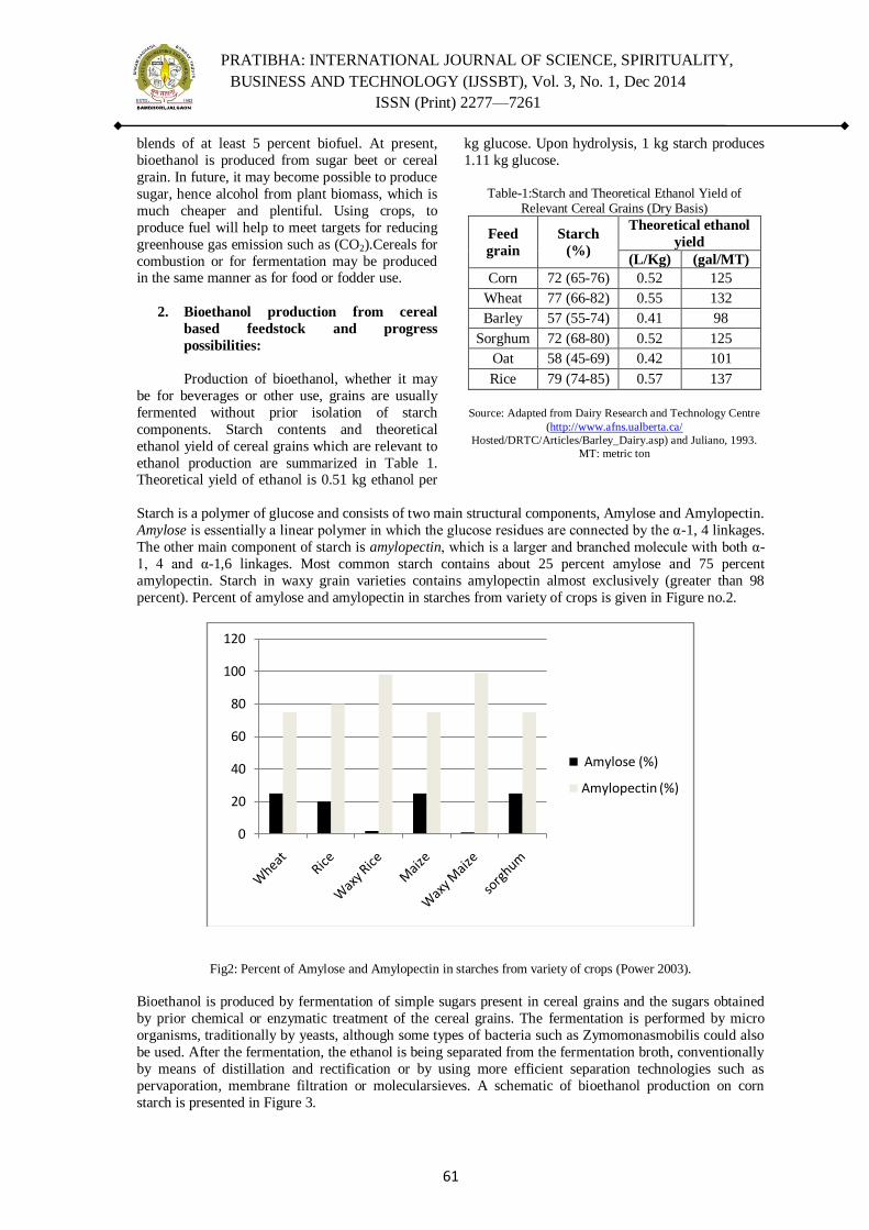
PRATIBHA: INTERNATIONAL JOURNAL OF SCIENCE, SPIRITUALITY,
BUSINESS AND TECHNOLOGY (IJSSBT), Vol. 3, No. 1, Dec 2014
ISSN (Print) 2277—7261
61
blends of at least 5 percent biofuel. At present,
bioethanol is produced from sugar beet or cereal
grain. In future, it may become possible to produce
sugar, hence alcohol from plant biomass, which is
much cheaper and plentiful. Using crops, to
produce fuel will help to meet targets for reducing
greenhouse gas emission such as (CO2).Cereals for
combustion or for fermentation may be produced in the same manner as for food or fodder use.
2. Bioethanol production from cereal
based feedstock and progress
possibilities:
Production of bioethanol, whether it may
be for beverages or other use, grains are usually
fermented without prior isolation of starch
components. Starch contents and theoretical
ethanol yield of cereal grains which are relevant to
ethanol production are summarized in Table 1. Theoretical yield of ethanol is 0.51 kg ethanol per
kg glucose. Upon hydrolysis, 1 kg starch produces
1.11 kg glucose.
Table-1:Starch and Theoretical Ethanol Yield of
Relevant Cereal Grains (Dry Basis)
Feed
grain
Starch
(%)
Theoretical ethanol
yield
(L/Kg) (gal/MT)
Corn 72 (65-76) 0.52 125
Wheat 77 (66-82) 0.55 132
Barley 57 (55-74) 0.41 98
Sorghum 72 (68-80) 0.52 125
Oat 58 (45-69) 0.42 101
Rice 79 (74-85) 0.57 137
Source: Adapted from Dairy Research and Technology Centre
(http://www.afns.ualberta.ca/
Hosted/DRTC/Articles/Barley_Dairy.asp) and Juliano, 1993.
MT: metric ton
Starch is a polymer of glucose and consists of two main structural components, Amylose and Amylopectin.
Amylose is essentially a linear polymer in which the glucose residues are connected by the α-1, 4 linkages.
The other main component of starch is amylopectin, which is a larger and branched molecule with both α-
1, 4 and α-1,6 linkages. Most common starch contains about 25 percent amylose and 75 percent
amylopectin. Starch in waxy grain varieties contains amylopectin almost exclusively (greater than 98
percent). Percent of amylose and amylopectin in starches from variety of crops is given in Figure no.2.
Fig2: Percent of Amylose and Amylopectin in starches from variety of crops (Power 2003).
Bioethanol is produced by fermentation of simple sugars present in cereal grains and the sugars obtained
by prior chemical or enzymatic treatment of the cereal grains. The fermentation is performed by micro
organisms, traditionally by yeasts, although some types of bacteria such as Zymomonasmobilis could also
be used. After the fermentation, the ethanol is being separated from the fermentation broth, conventionally
by means of distillation and rectification or by using more efficient separation technologies such as
pervaporation, membrane filtration or molecularsieves. A schematic of bioethanol production on corn
starch is presented in Figure 3.
0
20
40
60
80
100
120
Amylose (%)
Amylopectin (%)
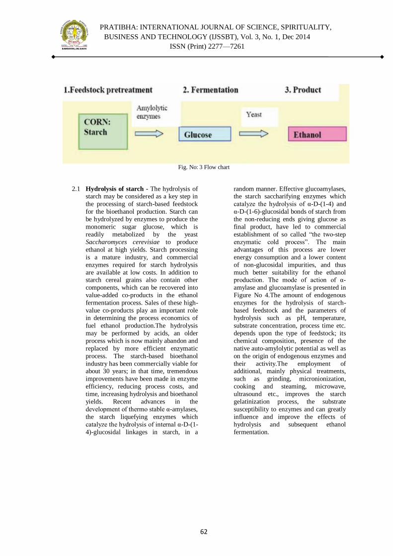
PRATIBHA: INTERNATIONAL JOURNAL OF SCIENCE, SPIRITUALITY,
BUSINESS AND TECHNOLOGY (IJSSBT), Vol. 3, No. 1, Dec 2014
ISSN (Print) 2277—7261
62
Fig. No: 3 Flow chart
2.1 Hydrolysis of starch - The hydrolysis of starch may be considered as a key step in
the processing of starch-based feedstock
for the bioethanol production. Starch can
be hydrolyzed by enzymes to produce the
monomeric sugar glucose, which is
readily metabolized by the yeast
Saccharomyces cerevisiae to produce
ethanol at high yields. Starch processing
is a mature industry, and commercial
enzymes required for starch hydrolysis
are available at low costs. In addition to starch cereal grains also contain other
components, which can be recovered into
value-added co-products in the ethanol
fermentation process. Sales of these high-
value co-products play an important role
in determining the process economics of
fuel ethanol production.The hydrolysis
may be performed by acids, an older
process which is now mainly abandon and
replaced by more efficient enzymatic
process. The starch-based bioethanol
industry has been commercially viable for about 30 years; in that time, tremendous
improvements have been made in enzyme
efficiency, reducing process costs, and
time, increasing hydrolysis and bioethanol
yields. Recent advances in the
development of thermo stable α-amylases,
the starch liquefying enzymes which
catalyze the hydrolysis of internal α-D-(1-
4)-glucosidal linkages in starch, in a
random manner. Effective glucoamylases, the starch saccharifying enzymes which
catalyze the hydrolysis of α-D-(1-4) and
α-D-(1-6)-glucosidal bonds of starch from
the non-reducing ends giving glucose as
final product, have led to commercial
establishment of so called ―the two-step
enzymatic cold process‖. The main
advantages of this process are lower
energy consumption and a lower content
of non-glucosidal impurities, and thus
much better suitability for the ethanol production. The mode of action of α-
amylase and glucoamylase is presented in
Figure No 4.The amount of endogenous
enzymes for the hydrolysis of starch-
based feedstock and the parameters of
hydrolysis such as pH, temperature,
substrate concentration, process time etc.
depends upon the type of feedstock; its
chemical composition, presence of the
native auto-amylolytic potential as well as
on the origin of endogenous enzymes and
their activity.The employment of additional, mainly physical treatments,
such as grinding, micronionization,
cooking and steaming, microwave,
ultrasound etc., improves the starch
gelatinization process, the substrate
susceptibility to enzymes and can greatly
influence and improve the effects of
hydrolysis and subsequent ethanol
fermentation.
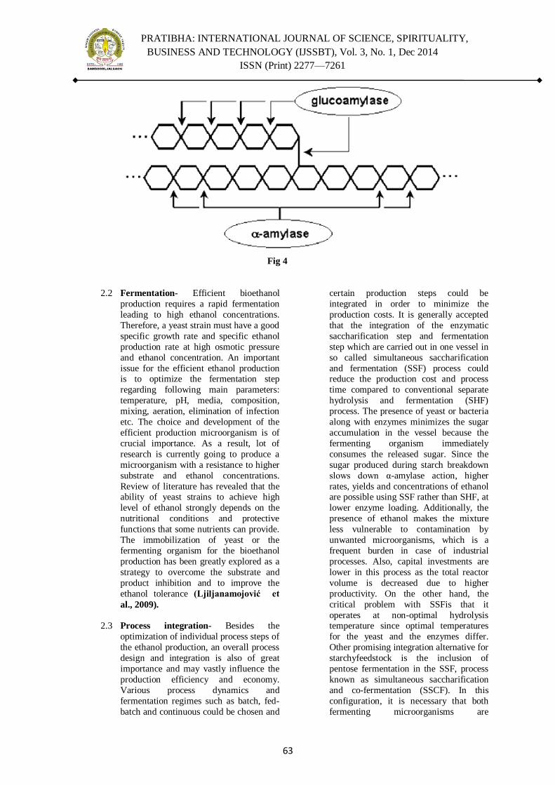
PRATIBHA: INTERNATIONAL JOURNAL OF SCIENCE, SPIRITUALITY,
BUSINESS AND TECHNOLOGY (IJSSBT), Vol. 3, No. 1, Dec 2014
ISSN (Print) 2277—7261
63
Fig 4
2.2 Fermentation- Efficient bioethanol
production requires a rapid fermentation
leading to high ethanol concentrations.
Therefore, a yeast strain must have a good
specific growth rate and specific ethanol
production rate at high osmotic pressure
and ethanol concentration. An important
issue for the efficient ethanol production is to optimize the fermentation step
regarding following main parameters:
temperature, pH, media, composition,
mixing, aeration, elimination of infection
etc. The choice and development of the
efficient production microorganism is of
crucial importance. As a result, lot of
research is currently going to produce a
microorganism with a resistance to higher
substrate and ethanol concentrations.
Review of literature has revealed that the ability of yeast strains to achieve high
level of ethanol strongly depends on the
nutritional conditions and protective
functions that some nutrients can provide.
The immobilization of yeast or the
fermenting organism for the bioethanol
production has been greatly explored as a
strategy to overcome the substrate and
product inhibition and to improve the
ethanol tolerance (Ljiljanamojović et
al., 2009).
2.3 Process integration- Besides the
optimization of individual process steps of
the ethanol production, an overall process
design and integration is also of great
importance and may vastly influence the
production efficiency and economy.
Various process dynamics and
fermentation regimes such as batch, fed-
batch and continuous could be chosen and
certain production steps could be
integrated in order to minimize the
production costs. It is generally accepted
that the integration of the enzymatic
saccharification step and fermentation
step which are carried out in one vessel in
so called simultaneous saccharification
and fermentation (SSF) process could reduce the production cost and process
time compared to conventional separate
hydrolysis and fermentation (SHF)
process. The presence of yeast or bacteria
along with enzymes minimizes the sugar
accumulation in the vessel because the
fermenting organism immediately
consumes the released sugar. Since the
sugar produced during starch breakdown
slows down α-amylase action, higher
rates, yields and concentrations of ethanol are possible using SSF rather than SHF, at
lower enzyme loading. Additionally, the
presence of ethanol makes the mixture
less vulnerable to contamination by
unwanted microorganisms, which is a
frequent burden in case of industrial
processes. Also, capital investments are
lower in this process as the total reactor
volume is decreased due to higher
productivity. On the other hand, the
critical problem with SSFis that it
operates at non-optimal hydrolysis temperature since optimal temperatures
for the yeast and the enzymes differ.
Other promising integration alternative for
starchyfeedstock is the inclusion of
pentose fermentation in the SSF, process
known as simultaneous saccharification
and co-fermentation (SSCF). In this
configuration, it is necessary that both
fermenting microorganisms are
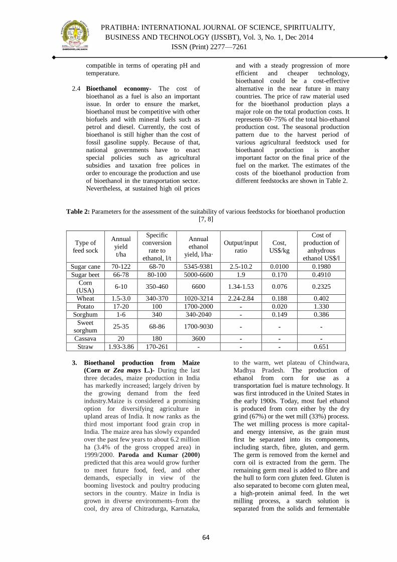
PRATIBHA: INTERNATIONAL JOURNAL OF SCIENCE, SPIRITUALITY,
BUSINESS AND TECHNOLOGY (IJSSBT), Vol. 3, No. 1, Dec 2014
ISSN (Print) 2277—7261
64
compatible in terms of operating pH and
temperature.
2.4 Bioethanol economy- The cost of
bioethanol as a fuel is also an important
issue. In order to ensure the market,
bioethanol must be competitive with other
biofuels and with mineral fuels such as petrol and diesel. Currently, the cost of
bioethanol is still higher than the cost of
fossil gasoline supply. Because of that,
national governments have to enact
special policies such as agricultural
subsidies and taxation free polices in
order to encourage the production and use
of bioethanol in the transportation sector.
Nevertheless, at sustained high oil prices
and with a steady progression of more
efficient and cheaper technology,
bioethanol could be a cost-effective
alternative in the near future in many
countries. The price of raw material used
for the bioethanol production plays a
major role on the total production costs. It
represents 60–75% of the total bio-ethanol production cost. The seasonal production
pattern due to the harvest period of
various agricultural feedstock used for
bioethanol production is another
important factor on the final price of the
fuel on the market. The estimates of the
costs of the bioethanol production from
different feedstocks are shown in Table 2.
Table 2: Parameters for the assessment of the suitability of various feedstocks for bioethanol production [7, 8]
Type of
feed sock
Annual
yield
t/ha
Specific
conversion
rate to
ethanol, l/t
Annual
ethanol
yield, l/ha·
Output/input
ratio
Cost,
US$/kg
Cost of
production of
anhydrous
ethanol US$/l
Sugar cane 70-122 68-70 5345-9381 2.5-10.2 0.0100 0.1980
Sugar beet 66-78 80-100 5000-6600 1.9 0.170 0.4910
Corn
(USA) 6-10 350-460 6600 1.34-1.53 0.076 0.2325
Wheat 1.5-3.0 340-370 1020-3214 2.24-2.84 0.188 0.402
Potato 17-20 100 1700-2000 - 0.020 1.330
Sorghum 1-6 340 340-2040 - 0.149 0.386
Sweet
sorghum 25-35 68-86 1700-9030 - - -
Cassava 20 180 3600 - - -
Straw 1.93-3.86 170-261 - - - 0.651
3. Bioethanol production from Maize
(Corn or Zea mays L.)- During the last
three decades, maize production in India has markedly increased; largely driven by
the growing demand from the feed
industry.Maize is considered a promising
option for diversifying agriculture in
upland areas of India. It now ranks as the
third most important food grain crop in
India. The maize area has slowly expanded
over the past few years to about 6.2 million
ha (3.4% of the gross cropped area) in
1999/2000. Paroda and Kumar (2000)
predicted that this area would grow further
to meet future food, feed, and other demands, especially in view of the
booming livestock and poultry producing
sectors in the country. Maize in India is
grown in diverse environments–from the
cool, dry area of Chitradurga, Karnataka,
to the warm, wet plateau of Chindwara,
Madhya Pradesh. The production of
ethanol from corn for use as a transportation fuel is mature technology. It
was first introduced in the United States in
the early 1900s. Today, most fuel ethanol
is produced from corn either by the dry
grind (67%) or the wet mill (33%) process.
The wet milling process is more capital-
and energy intensive, as the grain must
first be separated into its components,
including starch, fibre, gluten, and germ.
The germ is removed from the kernel and
corn oil is extracted from the germ. The
remaining germ meal is added to fibre and the hull to form corn gluten feed. Gluten is
also separated to become corn gluten meal,
a high-protein animal feed. In the wet
milling process, a starch solution is
separated from the solids and fermentable

PRATIBHA: INTERNATIONAL JOURNAL OF SCIENCE, SPIRITUALITY,
BUSINESS AND TECHNOLOGY (IJSSBT), Vol. 3, No. 1, Dec 2014
ISSN (Print) 2277—7261
65
sugars are produced from the starch. These
sugars are fermented to ethanol. Wet mill
facilities are true ―biorefineries‖,
producing a number of high-value
products. In the dry grind process, clean
corn is ground and mixed with water to
form a mash. The mash is cooked and
enzymes are added to convert starch to sugar. Then yeast is added to ferment the
sugars, producing a mixture containing
ethanol and solids. This mixture is then
distilled and dehydrated to create fuel-
grade ethanol. The solids remaining after
distillation are dried to produce distillers‘
dried grains with protein and are sold as an
animal feed supplement.
4. Bioethanol production from Sorghum-
Sorghum is an important drought-resistant
cereal crop, originally from Africa. Sorghum is ranked as the fifth largest
produced cereal in the world after wheat,
rice, barley and corn (Shewale and
Pandit, 2009). In Africa, China and India,
sorghum is a staple food, while in the
United States, Australia and South
America it is used for animal feed (Belton
and Taylor,2004). In some areas of Brazil,
sorghum has been increasingly planted
during the dry season between crops of
soybeans or cotton. Sorghum is valued because of its ability to grow in areas with
marginal rainfall and high temperatures
i.e., in semiarid tropical and subtropical
regions of the world, where it is difficult to
grow any other cereal. Also, because of its
relatively short growing season
requirements, it is suitable for double
cropping and crop rotation systems (Smith
and Frederiksen, 2000). Sorghum has a
relatively low cash value if sold directly as
feed grain (Fang and Hanna, 2002). To enhance the value of sorghum crops, new
industrial utility needs to be developed.
Sorghum grain is one of the most
important sources of carbohydrates.
Carbohydrates and fibres comprise
approximately 72% of sorghum grains. Its
starch component has similar properties to
corn starch, and can be used almost
interchangeably. Since there are hundreds
of sorghum hybrids available
commercially, if these feed stocks are
option for bioethanol production. The large variations in their composition will surely
affect the hydrolysis and fermentation
performance (Wang et al., 2008). Thus, it
is important for the ethanol industry and
sorghum producers to have appropriate
methods that accurately predict sorghum
ethanol yields and conversion efficiencies
(Zhao et al., 2009).
5. Conclusion
A significant progress and enhancement in the economy of bioethanol production on starch--
based raw materials may be obtained by the
process optimization of feedstock pretreatment and
ethanol fermentation itself, and by an adequate
utilization of the process byproducts. The
introduction of new pre-treatments such as
microwave and ultrasound can improve the starch
gelatinization process, the substrate susceptibility
to enzymes and greatly influence and improve the
effects of hydrolysis and subsequent ethanol
fermentation. In the domain of fermentation the
choice of the production microorganism, media optimization, and the choice of the most
appropriate process flow sheet (simultaneous
saccharification and fermentation, utilization of
immobilized yeasts, etc.) are significant for the
development of an efficient production process.
Thus, utilization of especially damaged cereal
grains for bioethanol production is the best option
for fossil fuel shortage.
References
[1]. K. Suresh,, N. Kiransree, L. Venkateswer Rao, Bio-
resource Technology, Utilization of damaged sorghum
and rice grains for ethanol production by simultaneous
saccharification and fermentation, Volume 68, Issue 3,
June 1999, Pages 301–304, doi:10.1016/S0960-
8524(98)00135-7.
[2]. C. Wrigley, I.L. Batey, Cereal Grains: Assessing and
Managing Quality, Wood head Publishing Series in
Food Science Technology and Nutrition, 2010
[3]. Dairy Research and Technology Centre, University of
Alberta, Barley grain for dairy
cattle.Availablefrom:(http://www.afns.ualberta.ca/Host
ed/DRTC/Articles/Barley_Dairy.asp)
[4]. Juliano, B.O.1993, ―Rice in human nutrition.‖ United
Nations Food and Agricultural Organization (FAO).
[5]. Power R(2003), enzymatic conversion of starch to
fermentable sugars. In KA Jaques, TP Lyons, D R Kels
all, eds, The Alcohol Textbook. Nottingham University
Press, Nottingham UK
[6]. Ljiljanamojović, Dušankapejin, Olgicagrujić,
Sinišamarkov, Jelenapejin, Maricarakin,
Majavukašinović, Svetlana nikolić, Dragišasavić,
Progress in the Production of Bio-ethanol on Starch-
Based Feed stocks, Chemical Industry & Chemical
Engineering Quarterly 15 (4) 211−226 (2009).
[7]. O.J. Sanchez, C.A. Cardona, Bio-resource. Technol. 99
(2008) 5270–5295
[8]. L. Mojović, D. Pejin, M. Lazić, in: Bio-ethanol as fuel
state of the art and perspectives, Faculty of
Technology, Leskovac, 2007, pp. 1-149 (in Serbian)
[9]. Paroda, R.S., and P. Kumar. 2000. Food production
and demand in South Asia. Agricultural Economics
Research Review 13(1):1-25.

PRATIBHA: INTERNATIONAL JOURNAL OF SCIENCE, SPIRITUALITY,
BUSINESS AND TECHNOLOGY (IJSSBT), Vol. 3, No. 1, Dec 2014
ISSN (Print) 2277—7261
66
[10]. Shewale, S. D. and Pandit, A. B., Enzymatic
Production of Glucose from Different Qualities of
Grain Sorghum and Application of Ultrasound to
Enhance the Yield. Carbohydrate Research, 344, pp.
52-60, 2009
[11]. Belton, P. S. and Taylor, J. R. N., Sorghum and
Millets: Protein Sources for Africa. Trends Food
Science and Technology, 15, 94-98 (2004).
[12]. Smith, C. W. and Frederiksen, R. A., Sorghum: Origin,
History, Technology and Production, P.III. Wiley, New
York (2000).
[13]. Fang, Q. and Hanna, M. A., Experimental Studies for
Levulinic Acid Production from Whole Kernel Grain
Sorghum. Bio-resource Technology, 81,187-192
(2002).
[14]. Wang, D., Bean, S., McLaren, J., Seib, P., Madl,
R.,Tuinstra, M., Shi, Y., Lenz, M., Wu, X., and Zhao,
R., Grain Sorghum is a Viable Feedstock for Ethanol
Production. Journal of Industrial Microbiology and
Biotechnology, 35, 313-320 (2008).
[15]. Zhao, R., Ban, S. R., Wang, D., Park, S. H., Schober,
T. J. and Wilson, J. D., Small-Scale Mashing Procedure
for Predicting Ethanol Yield of Sorghum Grain. Journal
of Cereal Science, 49,230-238 (2009).

PRATIBHA: INTERNATIONAL JOURNAL OF SCIENCE, SPIRITUALITY,
BUSINESS AND TECHNOLOGY (IJSSBT), Vol. 3, No. 1, Dec 2014
ISSN (Print) 2277—7261
67
A Critical Review on Low Temperature Solar Water Heater
Collectors
Ashish N. Sarode1, Atul A. Patil
2, Vijay H.Patil
3
1,2,3Deprtment of Mechanical Engineering, Godavari College of Engineering, Jalgaon – 425001, India.
Emails: [email protected], [email protected], [email protected]
Abstract: Energy application from the sun to
heat water is well known.The solar radiation
incident on the surface of the earth can be
conveniently utilized for the benefit of human
society. One of the popular devices that harness
the solar energy is solar hot water system
(SHWS).A solar water heater consists of collector
to collect solar energy and an insulated storage
tank to store hot water. The re-circulation water
through absorber panel in the collector help to
raises the temperature to 800C in a good sunny
day. This communications presents comparative
study of Flat plate collectors and Evacuated tube
collectors used in solar water heating system.
This indicates that the Evacuated tube collector
is more efficient than flat plate collector.
Keywords: Solar hot water system (SHWS),
absorber panel, solar collector.
I. INTRODUCTION
The sun is responsible for all of the earth energy. Plants use the sun's light to make food.
Decaying plants hundreds of millions of years ago
produced the coal, oil and natural gas that we use
today.Solar energy is created by light and heat
which is emitted by the sun, in the formof
electromagnetic radiationand now days we are able
to capture this radiation and turn it intousable
forms of solar energy such as heating or electricity
[1].
Solar energy is the sun's nuclear fusion
reactions within the continuous energygenerated. Earth's orbit, the average solar radiation intensity is
1367kw/m2.Circumference of the Earth's equator is
40000km, thus we can calculate theenergy the
earth gets is up to 173,000 TW. At sea level on the
standard peak intensity is 1kw/m2, a point on the
earth's surface 24h of the annual averageradiation
intensity is 0.20kw/m2, or roughly 102,000 TW of
energy [1], [2].
The total amount of solar energy
resources isten thousand times of the energy used
by humans, but the solar energy densityis low, and
it is influenced by location, season, which is a major problem ofdevelopment and utilization of
solar energy [4].
Solar energy can be used by four
technological processes, Chemical, Electrical,
Thermal and Mechanical energy [13].Chemical
process, through photosynthesis, maintains life on
earth by producing food and converting CO2 to O2.
Electrical process, using photovoltaic converters,
provides power for spacecraft and is used in many
terrestrial applications. Thermal process can be
used to provide much of the thermal energy
required for solar water heating and building heating. Another one form of convertedsolar
radiation is mechanical energy as wind and water
steams [14].
The most important and most expensive
single component of an active solar energy system
is thecollector field, which may be performed in a
several versions, as from constructions of solar
collectors, as of collector configuration. Solar
collectors are the heart of most solar energy
systems. The collector absorbs thesun‘s light
energy and changes it into heat energy.
Solar hot water systems function as heat exchangers. They receive solar radiant energy and
transfer it to the flowing fluid. The performance of
solar systems varies as the design variables
change, so it is therefore necessary to identify the
parameters affecting this design and the
operational variables.Solar water heating has been
around for many years because it is the easiest way
to use the sun to save energy and money. One of
the earliest documented cases of solar energy use
involved pioneers moving west after the Civil War.
They would place a cooking pot filled with cold water in the sun all day to have heated water in the
evening.
The first solar water heater that resembles
the concept still in use today was a metal tank that
was painted black and placed on the roof where it
was tilted toward the sun. The concept worked,
but it usually took all day for the water to heat,
then, as soon as the sun went down, it cooled off
quickly because the tank was not insulated.
The roles of thermal collectors are simple
sit in the sun, absorb and transfer heat, and do it
reliably for decades. But to fill their roles efficiently, collectors need to absorb a high level of
solar radiation, while minimizing losses from

PRATIBHA: INTERNATIONAL JOURNAL OF SCIENCE, SPIRITUALITY,
BUSINESS AND TECHNOLOGY (IJSSBT), Vol. 3, No. 1, Dec 2014
ISSN (Print) 2277—7261
68
reflection and heat loss to the surrounding
environment.
II. SOLAR WATER HEATING SYSTEM
Solar water heating systems can be broadly divided
into three main parts:
1. Solar collector that receive and transfer the sun's radiant energy into thermal energy in
the working fluid.
2. System of working fluid channel or pipe
diverter, which is the part that connects the
collector to the storage.
3. Fluid storage tank that is part of the store
and hold hot water.
Classifications of solar collectors according to
concentration degree are as given bellow [5]. Table No. 1 Classifications of solar collectors according
to concentration degree
Category
ºC
Example Temper
ature
range,
Efficien
cy, %
No
concentrat
ion
Flat-plate
Evacuated
tube
up to 75
up to 200
30 – 50
Medium concentration Parabolic cylinder
150 - 500
50 – 70
High
concentrat
ion
Parabodial 1500 and
more
60 - 75
The majority of solar thermal collectors for low
temperature water heater are Flat plate solar
thermal collector andEvacuated tube solar thermal
collector.
III.TYPES OF SOLAR THERMAL
COLLECTOR FOR LOW TEMERATURE
RANGE
1. The Flat Plate Solar Collector
A Flat plate solar collector is required to
absorb solar radiation and to transfer the absorbed
energy into a heat transfer fluid with a minimum of
heat loss. In assessing the performance of a
collector it is therefore important both to determine
its ability to absorb solar radiationand to
characterise its heat losses [3]. The principal components and losses are shown in Figure.
Fig No.1 Solar Radiation Process.
Fig No.2 Flat plate collector.
The ability of a collector to absorb solar
radiation is largely determined by the optical
properties of its cover and absorber surface.
However, there are also losses, which may be considered as input losses, associated with the
transfer of heat from the absorber surface into the
heat transfer fluid. These are influenced by the
design of the absorber fluid passageways.
A collector loses heat from its front, its
back and its sides. The back and side losses from a
flat plate collector can be minimised by the use of
insulation. The heat losses from the front of a flat
plate collector are usually the largest component of
the overall heat losses. They occur in the form of
convection and thermal radiation from the front cover to the environment and can be reduced by
designing thecollector in such a way that the
temperature of the front cover is kept low. This can
be achieved by minimising the heat transfer
between the absorber and the outer cover. The
convective heat transfer between the absorber and
the outer cover can be reduced by using a multiple
glazing system or by evacuating the space over the
absorber. The radiative heat transfer from the
absorber to the cover can be reduced by the use of
selective surfaces.The main advantage of flat plate
solar thermal collectors is their low equipment cost. Under the current market, the cost of a flat
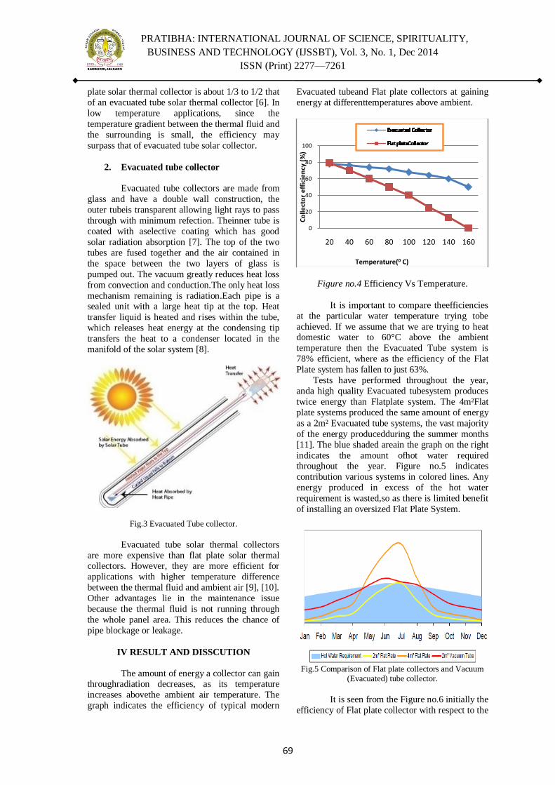
PRATIBHA: INTERNATIONAL JOURNAL OF SCIENCE, SPIRITUALITY,
BUSINESS AND TECHNOLOGY (IJSSBT), Vol. 3, No. 1, Dec 2014
ISSN (Print) 2277—7261
69
plate solar thermal collector is about 1/3 to 1/2 that
of an evacuated tube solar thermal collector [6]. In
low temperature applications, since the
temperature gradient between the thermal fluid and
the surrounding is small, the efficiency may
surpass that of evacuated tube solar collector.
2. Evacuated tube collector
Evacuated tube collectors are made from
glass and have a double wall construction, the
outer tubeis transparent allowing light rays to pass
through with minimum refection. Theinner tube is
coated with aselective coating which has good
solar radiation absorption [7]. The top of the two
tubes are fused together and the air contained in
the space between the two layers of glass is
pumped out. The vacuum greatly reduces heat loss
from convection and conduction.The only heat loss
mechanism remaining is radiation.Each pipe is a sealed unit with a large heat tip at the top. Heat
transfer liquid is heated and rises within the tube,
which releases heat energy at the condensing tip
transfers the heat to a condenser located in the
manifold of the solar system [8].
Fig.3 Evacuated Tube collector.
Evacuated tube solar thermal collectors
are more expensive than flat plate solar thermal collectors. However, they are more efficient for
applications with higher temperature difference
between the thermal fluid and ambient air [9], [10].
Other advantages lie in the maintenance issue
because the thermal fluid is not running through
the whole panel area. This reduces the chance of
pipe blockage or leakage.
IV RESULT AND DISSCUTION
The amount of energy a collector can gain throughradiation decreases, as its temperature
increases abovethe ambient air temperature. The
graph indicates the efficiency of typical modern
Evacuated tubeand Flat plate collectors at gaining
energy at differenttemperatures above ambient.
Figure no.4 Efficiency Vs Temperature.
It is important to compare theefficiencies
at the particular water temperature trying tobe
achieved. If we assume that we are trying to heat domestic water to 60°C above the ambient
temperature then the Evacuated Tube system is
78% efficient, where as the efficiency of the Flat
Plate system has fallen to just 63%.
Tests have performed throughout the year,
anda high quality Evacuated tubesystem produces
twice energy than Flatplate system. The 4m²Flat
plate systems produced the same amount of energy
as a 2m² Evacuated tube systems, the vast majority
of the energy producedduring the summer months
[11]. The blue shaded areain the graph on the right
indicates the amount ofhot water required throughout the year. Figure no.5 indicates
contribution various systems in colored lines. Any
energy produced in excess of the hot water
requirement is wasted,so as there is limited benefit
of installing an oversized Flat Plate System.
Fig.5 Comparison of Flat plate collectors and Vacuum (Evacuated) tube collector.
It is seen from the Figure no.6 initially the
efficiency of Flat plate collector with respect to the
0
20
40
60
80
100
20 40 60 80 100 120 140 160
Co
llect
or
eff
icie
ncy
(%
)
Temperature(0 C)
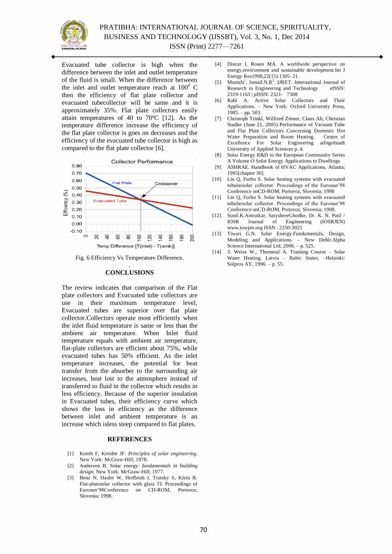
PRATIBHA: INTERNATIONAL JOURNAL OF SCIENCE, SPIRITUALITY,
BUSINESS AND TECHNOLOGY (IJSSBT), Vol. 3, No. 1, Dec 2014
ISSN (Print) 2277—7261
70
Evacuated tube collector is high when the
difference between the inlet and outlet temperature
of the fluid is small. When the difference between
the inlet and outlet temperature reach at 1000 C
then the efficiency of flat plate collector and
evacuated tubecollector will be same and it is
approximately 35%. Flat plate collectors easily
attain temperatures of 40 to 70ºC [12]. As the temperature difference increase the efficiency of
the flat plate collector is goes on decreases and the
efficiency of the evacuated tube collector is high as
compared to the flat plate collector [6].
Fig. 6 Efficiency Vs Temperature Difference. .
CONCLUSIONS
The review indicates that comparison of the Flat
plate collectors and Evacuated tube collectors are
use in their maximum temperature level,
Evacuated tubes are superior over flat plate
collector.Collectors operate most efficiently when
the inlet fluid temperature is same or less than the
ambient air temperature. When Inlet fluid temperature equals with ambient air temperature,
flat-plate collectors are efficient about 75%, while
evacuated tubes has 50% efficient. As the inlet
temperature increases, the potential for heat
transfer from the absorber to the surrounding air
increases, heat lost to the atmosphere instead of
transferred to fluid in the collector which results in
less efficiency. Because of the superior insulation
in Evacuated tubes, their efficiency curve which
shows the loss in efficiency as the difference
between inlet and ambient temperature is an
increase which isless steep compared to flat plates.
REFERENCES
[1] Kreith F, Kreider JF. Principles of solar engineering.
New York: McGraw-Hill; 1978.
[2] Anderson B. Solar energy: fundamentals in building
design. New York: McGraw-Hill; 1977.
[3] Benz N, Hasler W, Hetfleish J, Tratzky S, Klein B.
Flat-platesolar collector with glass TI. Proceedings of
Eurosun‘98Conference on CD-ROM, Portoroz,
Slovenia; 1998.
[4] Dincer I, Rosen MA. A worldwide perspective on
energy,environment and sustainable development.Int J
Energy Res1998;22(15):1305–21.
[5] Mustafa1, Ismail.N.R
2. IJRET: International Journal of
Research in Engineering and Technology eISSN:
2319-1163 | pISSN: 2321- 7308
[6] Rabl A. Active Solar Collectors and Their
Applications. – New York: Oxford University Press,
1985. – pp. 503.
[7] Christoph Trinkl, Wilfried Zörner, Claus Alt, Christian
Stadler (June 21, 2005) Performance of Vacuum Tube
and Flat Plate Collectors Concerning Domestic Hot
Water Preparation and Room Heating. Centre of
Excellence For Solar Engineering atIngolstadt
University of Applied Sciences p. 4.
[8] Solar Energy R&D in the European Community Series
A Volume O Solar Energy Applications to Dwellings
[9] ASHRAE. Handbook of HVAC Applications, Atlanta;
1995[chapter 30].
[10] Lin Q, Furbo S. Solar heating systems with evacuated
tubularsolar collector. Proceedings of the Eurosun‘98
Conference onCD-ROM, Portoroz, Slovenia; 1998
[11] Lin Q, Furbo S. Solar heating systems with evacuated
tubularsolar collector. Proceedings of the Eurosun‘98
Conference onCD-ROM, Portoroz, Slovenia; 1998.
[12] Sunil.K.Amrutkar, SatyshreeGhodke, Dr. K. N. Patil /
IOSR Journal of Engineering (IOSRJEN)
www.iosrjen.org ISSN : 2250-3021
[13] Tiwari G.N. Solar Energy.Fundamentals, Design,
Modeling and Applications. – New Dehli:Alpha
Science International Ltd, 2006. – p. 525.
[14] 3. Weiss W., Themessl A. Training Course – Solar
Water Heating. Latvia – Baltic States. –Helsinki:
Solpros AY, 1996. – p. 55.
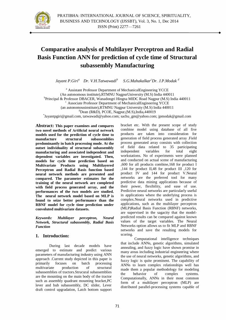
PRATIBHA: INTERNATIONAL JOURNAL OF SCIENCE, SPIRITUALITY,
BUSINESS AND TECHNOLOGY (IJSSBT), Vol. 3, No. 1, Dec 2014
ISSN (Print) 2277—7261
71
Comparative analysis of Multilayer Perceptron and Radial
Basis Function ANN for prediction of cycle time of Structural
subassembly Manufacturing
Jayant P.Giria
Dr. V.H.Tatwawadib S.G.Mahakalkar
cDr. J.P.Modak
d
a Assistant Professor Department of MechanicalEngineering YCCE
(An autonomous institute),RTMNU NagpurUniversity (M.S) India 440011 bPrincipal & Professor DBACER, Wanadongri Hingna MIDC Road Nagpur (M.S) India 440011
c Associate Professor Department of MechanicalEngineering YCCE
(an autonomousinstitute),RTMNU Nagpur University (M.S) India 440011 dDean (R&D), PCOE, Nagpur,(M.S),India,440019
*[email protected], [email protected]; [email protected]; [email protected]
Abstract: This paper examines and compares
two novel methods of Artificial neural network
models used for the prediction of cycle time to
manufacture structural subassemblies
predominantly in batch processing mode. At the
outset individuality of structural subassembly
manufacturing and associated independent and
dependent variables are investigated. Then,
models for cycle time prediction based on
Multivariate Products using Multilayered
Perceptron and Radial Basis function based
neural network methods are presented and
compared. The parameter estimates for the
training of the neural network are completed
with field process generated array, and the
performances of the two models are studied.
The neural network model based on MLP is
found to seize better performance than the
RBNF model for cycle time prediction under
convoluted multivariate datasets.
Keywords: Multilayer perceptron, Neural
Network, Structural subassembly, Radial Basis
Function
1. Introduction:
During last decade models have
emerged to estimate and predict various
parameters of manufacturing industry using ANN
approach .Current study depicted in this paper is
primarily focuses on batch processing
multivariate production of structural
subassemblies of tractors.Strucural subassemblies
are the mounting on the main body of the tractor
such as assembly quadrant mounting bracket,PC
lever and hub subassembly, DC slider, Lever
draft control upgradation, Latch bottom support
bracket etc. With the present scope of study
combine model using database of all five
products are taken into consideration for
generation of field process generated array .Field
process generated array consists with collection
of field data related to 35 participating independent variables for total eight
workstations. No of experiments were planned
and conducted on actual scene of manufacturing
,600 for all products combine,168 for product I
,144 for product II,48 for product III ,120 for
product IV and 144 for product V.Neural
networks are the preferred tool for many
predictive data mining applications because of
their power, flexibility, and ease of use.
Predictive neural networks are particularly useful
in applications where the underlying process is
complex.Neural networks used in predictive applications, such as the multilayer perceptron
(MLP)Radial Basis Function (RBNF) networks,
are supervised in the sagacity that the model-
predicted results can be compared against known
values of the target variables. The Neural
Networks option allows us to fit MLP and RBNF
networks and save the resulting models for
scoring.
Computational intelligence techniques
that include ANNs, genetic algorithms, simulated
annealing, and fuzzy logic have shown promise in many areas including industrial engineering where
the use of neural networks, genetic algorithms, and
fuzzy logic is quite prominent. The capability of
ANNs to learn complex relationships well has
made them a popular methodology for modeling
the behavior of complex systems.
Computationally, ANNs in their most common
form of a multilayer perceptron (MLP) are
distributed parallel-processing systems capable of
PRATIBHA: INTERNATIONAL JOURNAL OF SCIENCE, SPIRITUALITY,
BUSINESS AND TECHNOLOGY (IJSSBT), Vol. 3, No. 1, Dec 2014
ISSN (Print) 2277—7261
72
a fault tolerant and efficient learning and are
resistant to noise and disturbances. They are
connectionist structures composed of nodes called
neurons and arcs connecting the neurons with
weights associated with the arcs. Weights are
adaptable and are the main learning parameters of
the network. The network learns typically by using
a backpropagation learning algorithm (Rumelhart, Hinton, & Williams, 1986) that updates the
weights. The network has generally three types of
layers called input, output, and hidden layers. The
information is presented in a preprocessed or raw
format into the input layer of the network and the
predictions are obtained at the output layer of the
network.
2. Literature Review:
[Timothy James Stich, Dr. Julie K.
Spoerre & Dr. Tomás Velasco,2000] In their paper
on ―The Application of Artificial Neural Networks to Monitoring and Control of an Induction
Hardening Process‖ systematically investigated
thorough literature, according to them ,Artificial
neural networks (ANNs) are excellent tools for
complex manufacturing processes that have many
variables and complex interactions. Neural
networks have provided a means of successfully
controlling complex Processes [(Toosi and Zhu
1995, Hubick 1992,Hoskins and Himmelblau
1992,Coit and Smith 1995, Fan and Wu 1995,and
Chovan, Catfolis and Meert 1996)].Other
applications of neural networks include bearing fault classification [Spoerre, 1997], turning,
tapping, and welding comparisons [Du, Elbestawi,
and Wu 1995],acoustic emission for tool condition
monitoring [Toosi and Zhu 1995], temperature
control in a continuous-stirred-tank reactor
[Hoskins and Himmelblau 1992], and monitoring
of chip production and cutting-tool wear [Hubick
1992]. [Pham and Oztemel (1994)] used an
integrated neural network-based pattern recognizer
and expert system for analyzing and interpreting
control charts. In another application, artificially intelligent process control functions based on a
unique combination of rule-based expert systems
and neural networks were developed to control a
complex pulp and paper process [Beaverstock
1993].
[Smith, A. E., & Mason, A. K. 1997]A
new method of estimating cost is through the use
of artificial neural networks or ANNs. One major
benefit of using a neural network is its ability to
comprehend and conjure up multifarious functions.
However, one of the current drawbacks to such use
is that as the complexity of the function increases, more training data becomes necessary if the
function is to be implicit as well as possible. This
meticulous disadvantage is a factor for any method
but is especially present with neural networks as it
requires the data to be split into multiple
subsets.Neural networks are used to simulate more
complex functions than older methods, such as
linear regression, making the amount of data
available increasingly important. Production data,
part designs, and part costs from a large aircraft engine manufacturer were used to train and test a
neural network. Two different part families, shafts
and cases, were evaluated, which represent two
different levels of part complexity [John D.
Dowler, 2008].Little work has been published on
using real world data to train and test a neural
network that can produce a cost estimate. To date,
those studies available show ANNs promising
ability to understand complex models and provide
a superior cost estimate when compared to
estimation methods such as linear regression
[Smith, A. E., & Mason, A. K. 1997]. [Marco Garetti, Marco Taisch, 2010] in
their paper mentioned mottled applications cover a
great number of industrial engineering domains
with different degrees of innovation. Examples
range from production scheduling to process
control [ Currie and Leclair 1993, Rogers and
Dagli1996] , from image recognition [ Huang et al.
1992] to signal processing [ Widrow et al . 1994] ,
from system identification [ Pollard et al . 1992] to
metal cutting [ Nagasaka et al. 1995, Yan et al .
1995] , from inspection [ Hou et al.1993] to forecasting, from product design [ Venugopal and
Narendran 1992, Wu 1993] to plant design and
location [ Shtub and Zimerman 1993,
Vaithyanathan et al . 1996] , from robot control to
system diagnosis [ Huang and Wang 1993, L in et
al. 1995] .
As mentioned and discussed by [Brad
Warner and Manavendra Misra, 1996] several
authors have done comparison studies between
statistical methods and neural networks [Hruschka
1993; Wu and Yen 1992]. These works have a propensity to focus on performance comparisons
and use specific problems as examples. There are a
number of good introductory articles on neural
networks, usually located in various trade journals.
For instance, [Lippmann (1987)] provides an
excellent overview of neural networks for the
signal processing community. There are also a
number of good introductory books on neural
networks, with [Hertz, Krogh, and Palmer (1991)]
providing a good mathematical description,[ Smith
(1993)] explaining backpropagation in an applied
setting, and [Freeman (1994)] using examples and code to explain neural networks. There have also
been papers relating neural networks and statistical
methods [Buntine and Weigend 1991; Ripley
1992; Sarle 1994; Werbos 1991]. One of the best

PRATIBHA: INTERNATIONAL JOURNAL OF SCIENCE, SPIRITUALITY,
BUSINESS AND TECHNOLOGY (IJSSBT), Vol. 3, No. 1, Dec 2014
ISSN (Print) 2277—7261
73
for a general overview is [Ripley (1993)]. [Frans
Vainio, Michael Maier, Timo Knuutila, Esa
Alhoniemi, 2009]According to cited literature of
this paper when considering possible methods for
estimating the operation times of manufacturing
machines, one can rely on statistical techniques.
Common nonlinear regression methods are well
known in the classical statistics literature [Hald (1967)].In recent years; neural networks have
gained much esteem due to their flexibility,
resourcefulness and simplicity. There are many
different types of neural networks supporting
nonlinear regression, e.g. MLP (multi-layer
perceptron), RBF (radial basis function) and SVM
(support vector machine)[Bishop (1995)]. Each of
these methods has strengths and weaknesses. It
turns out that conventional learning methods are
prone to overfitting when the number of hidden
units of the network is large in relation to the
number of training cases. In particular multiple regression (MR)
analysis (Edwardset al., 1999c). The great
advantage of regression is that it has an established
confirmation of use within the edifice research
community (Akintoye and Skitmore, 1994;
Akinsola, 1997). More recent studies have utilized
the artificial intelligent forecasting technique
``neural networks'' (more specifically, the
multilayer perceptron) (Edwards and Holt, 1999).
This was similarly successful in the prediction of
the hourly maintenance cost of tracked hydraulic excavators operating in the open cast mining
industry (Edwards et al., 1999b). However, in
order to weigh the success (or otherwise) of either
technique, a comparative analysis of prediction
performance must be made (Hua, 1996). For the
case, (Brass 1994) and (Smith and Mason 1997)
used multiple linear regressions to estimate the
product costs. However, their analysis did not
consider multicollinearity, heteroskedasticity, and
specification error and did not discuss the
possibility of adopting other regression models. Davim (2003) established correlations between the
response and process parameters using multiple
linear regression analysis (RA) technique. [Dr
Maria Karanika, 2009] Elaborate the center of
attention of the work- health relationship using
neural network and regression analysis and prime
focus was to establish whether artificial neural
networks would provide better fit than the time-
honored multiple linear regression analysis in
modelling the relationship between work
characteristics and work-related health. According
to author there would be differences in (1) variance explained between the linear regression models
and the neural networks, and (2) the relative
positioning of the predictors in the architecture of
the models. Inference models used in industry can
be broadly classified as parametric models,
analogous models and detailed models. Parametric
estimation is the generation and application of
equations that describe relationships between cost
schedules and measurable attributes of a system
that must be brought forth, sustained and retired
[Dean, 1995]. [Zhang, 1992] investigated a model
in which the input of each stage consists of a vector of m quality characteristics, X=(x1, x2. . .
xm)T, whose output is the preferred quality
characteristic or quality of the product Y. To
control such a process, Zhang proposed an
expansion of the univariate cause-selecting chart,
which he named the multivariate cause-selecting
chart (MCSC).
Cook and Chiu [1998] used the radial
basis function (RBF) neural networks trained by
the least-mean squares algorithm for statistical
process control of correlated processes. The trained
RBF neural networks were used to separate the shifted and unshifted correlated papermaking and
viscosity data in literature. The neural networks
successfully identified data that were shifted 1.5
and 2 standard deviations from non shifted data for
both the papermaking and viscosity processes. The
network for the papermaking data was able to also
classify shifts of one standard deviation, while the
traditional statistical process control (SPC)
technique cannot achieve this because it requires a
large average run length. Above mentioned
literature shows insightful porch of ANN and regression for diversified domains.
Baillie and Mathew [1994]‟s results in
diagnosing faults of rolling element bearings
indicated that backpropagation (BP) neural
networks generally outperformed the radial basis
functions (RBF). McCormick and Nandi [1996]
used multi-layer perceptron and radial basis
function neural networks to classify the condition
of a small rotating machine. It was found that both
networks achieved similar success in fault
classification. However RBF networks could be
trained in a significantly shorter length of time.
Multilayer perceptrons (MLP) however required fewer neurons and were faster in recall operation.
Meesad and Yen [2000] applied MLP and
Learning Vector Quantization (LVQ) classifiers to
diagnosing faults in gears, bearings, and shafts. It
was proven that these two neural networks were
successful while they required off-line training and
iterative presentation of the training data. They
were cumbersome when applied to pattern
classification problems that needed fast, on-line,
real-time, incremental learning.
3. Field experimentation: Representation of the actual corporeal
system for structural subassembly manufacturing
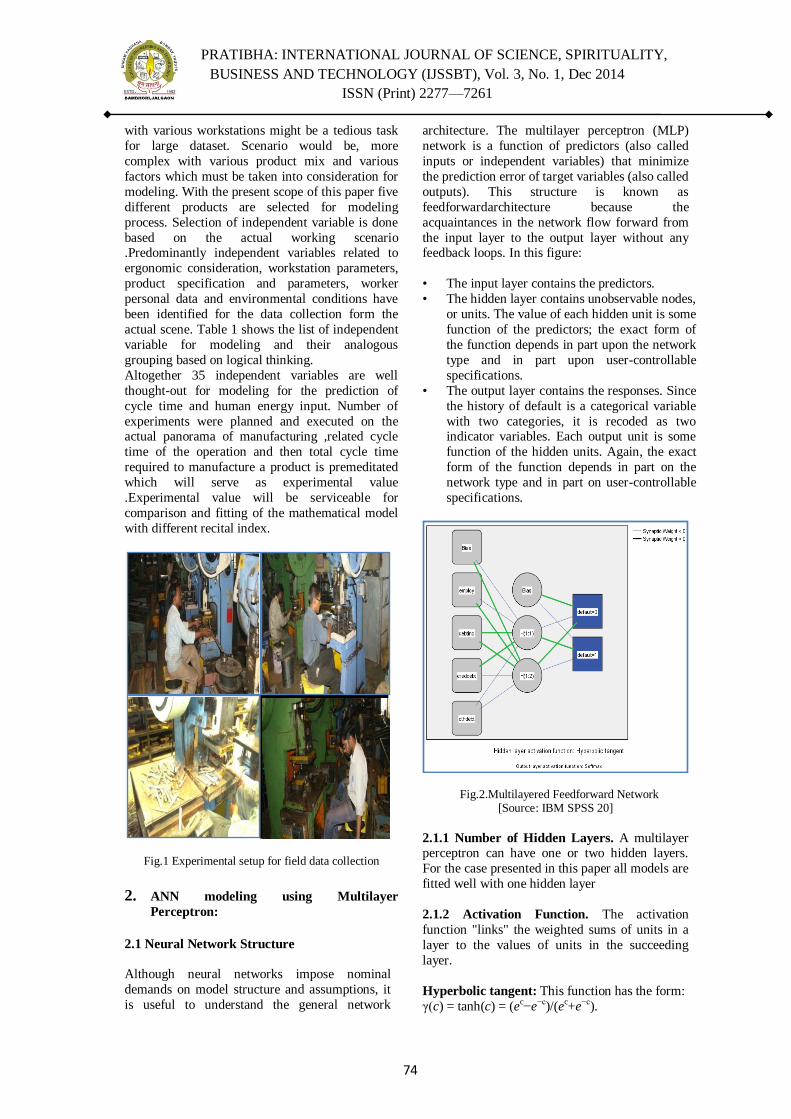
PRATIBHA: INTERNATIONAL JOURNAL OF SCIENCE, SPIRITUALITY,
BUSINESS AND TECHNOLOGY (IJSSBT), Vol. 3, No. 1, Dec 2014
ISSN (Print) 2277—7261
74
with various workstations might be a tedious task
for large dataset. Scenario would be, more
complex with various product mix and various
factors which must be taken into consideration for
modeling. With the present scope of this paper five
different products are selected for modeling
process. Selection of independent variable is done
based on the actual working scenario .Predominantly independent variables related to
ergonomic consideration, workstation parameters,
product specification and parameters, worker
personal data and environmental conditions have
been identified for the data collection form the
actual scene. Table 1 shows the list of independent
variable for modeling and their analogous
grouping based on logical thinking.
Altogether 35 independent variables are well
thought-out for modeling for the prediction of
cycle time and human energy input. Number of
experiments were planned and executed on the actual panorama of manufacturing ,related cycle
time of the operation and then total cycle time
required to manufacture a product is premeditated
which will serve as experimental value
.Experimental value will be serviceable for
comparison and fitting of the mathematical model
with different recital index.
Fig.1 Experimental setup for field data collection
2. ANN modeling using Multilayer
Perceptron:
2.1 Neural Network Structure
Although neural networks impose nominal
demands on model structure and assumptions, it
is useful to understand the general network
architecture. The multilayer perceptron (MLP)
network is a function of predictors (also called
inputs or independent variables) that minimize
the prediction error of target variables (also called
outputs). This structure is known as
feedforwardarchitecture because the
acquaintances in the network flow forward from
the input layer to the output layer without any feedback loops. In this figure:
• The input layer contains the predictors.
• The hidden layer contains unobservable nodes,
or units. The value of each hidden unit is some
function of the predictors; the exact form of
the function depends in part upon the network
type and in part upon user-controllable
specifications.
• The output layer contains the responses. Since
the history of default is a categorical variable
with two categories, it is recoded as two indicator variables. Each output unit is some
function of the hidden units. Again, the exact
form of the function depends in part on the
network type and in part on user-controllable
specifications.
Fig.2.Multilayered Feedforward Network [Source: IBM SPSS 20]
2.1.1 Number of Hidden Layers. A multilayer perceptron can have one or two hidden layers.
For the case presented in this paper all models are
fitted well with one hidden layer
2.1.2 Activation Function. The activation
function "links" the weighted sums of units in a
layer to the values of units in the succeeding
layer.
Hyperbolic tangent: This function has the form:
γ(c) = tanh(c) = (ec−e−c)/(ec+e−c).

PRATIBHA: INTERNATIONAL JOURNAL OF SCIENCE, SPIRITUALITY,
BUSINESS AND TECHNOLOGY (IJSSBT), Vol. 3, No. 1, Dec 2014
ISSN (Print) 2277—7261
75
It takes real-valued arguments and transformsthem
to the range (–1, 1). When automatic architecture
selection is used, this is the activation function for
all units in the hidden layers.Hypebolic tangential
function is utilized as activation function for
present study [Handbook of SPSS 20, IBM].
2.2 Multilayered perceptron modeling
2.2.1 Sample ANN model with base variable as
input and cycle time output for all products:
ANN equation for basic variables as input and
production cycle time as output is formulated as
follows:
X1,1= (e1*sum(Layer1Cell0) - e-1*sum(Layer1Cell0) ) / (
e1*sum(Layer1Cell0) + e-1*sum(Layer1Cell0) )
Where sum (Layer1cell0) =0.24*X0,1-0.43*X0,2 –
0.307*X0,3+0.17*X0,4+0.1888*X0,5-0.4*X0,6
+0.24* X0,7+0.4* X0,8+0.02* X0,9-0.074* X0,10-
0.023* X0,11+0.15* X0,12+0.099* X0,13+0.02*
X0,14+0.33* X0,15-0.421* X0,16+0.29* X0,17-0.009*
X0,18+0.04* X0,19+0.077* X0,20+0.471* X0,21-
0.146* X0,22-0.363* X0,23-0.417* X0,24+0.163*
X0,25-0.237* X0,26-0.329* X0,27+0.389* X0,28+0.196* X0,29+0.18* X0,30-0.359* X0,31+0.04*
X0,32-0.096* X0,33-0.0321* X0,34 -0.228* X0,35-
0.421
X1,2= (e1*sum(Layer1Cell1) - e-1*sum(Layer1Cell1) ) / (
e1*sum(Layer1Cell1) + e-1*sum(Layer1Cell1) )
Where sum (Layer1cell1) = 0.24*X0,1-0.43*X0,2 –
0.307*X0,3+0.17*X0,4+0.1888*X0,5-0.4*X0,6
+0.24* X0,7+0.4* X0,8+0.02* X0,9-0.074* X0,10-
0.023* X0,11+0.15* X0,12+0.099* X0,13+0.02*
X0,14+0.33* X0,15-0.421* X0,16+0.29* X0,17-0.009*
X0,18+0.04* X0,19+0.077* X0,20+0.471* X0,21-0.146* X0,22-0.363* X0,23-0.417* X0,24+0.163*
X0,25-0.237* X0,26-0.329* X0,27+0.389*
X0,28+0.196* X0,29+0.18* X0,30-0.359* X0,31+0.04*
X0,32-0.096* X0,33-0.0321* X0,34 -0.228* X0,35-
0.433
X1,3= (e1*sum(Layer1Cell2) - e-1*sum(Layer1Cell2) ) / (
e1*sum(Layer1Cell2) + e-1*sum(Layer1Cell2) )
Where sum (Layer1cell2) =0.24*X0,1-0.43*X0,2 –
0.307*X0,3+0.17*X0,4+0.1888*X0,5-0.4*X0,6
+0.24* X0,7+0.4* X0,8+0.02* X0,9-0.074* X0,10-0.023* X0,11+0.15* X0,12+0.099* X0,13+0.02*
X0,14+0.33* X0,15-0.421* X0,16+0.29* X0,17-0.009*
X0,18+0.04* X0,19+0.077* X0,20+0.471* X0,21-
0.146* X0,22-0.363* X0,23-0.417* X0,24+0.163*
X0,25-0.237* X0,26-0.329* X0,27+0.389*
X0,28+0.196* X0,29+0.18* X0,30-0.359* X0,31+0.04*
X0,32-0.096* X0,33-0.0321* X0,34 -0.228*
X0,35+0.459
X1,4= (e1*sum(Layer1Cell3) - e-1*sum(Layer1Cell3) ) / (
e1*sum(Layer1Cell3) + e-1*sum(Layer1Cell3) )
Where sum (Layer1cell4) =0.24*X0,1-0.43*X0,2 –
0.307*X0,3+0.17*X0,4+0.1888*X0,5-0.4*X0,6
+0.24* X0,7+0.4* X0,8+0.02* X0,9-0.074* X0,10-
0.023* X0,11+0.15* X0,12+0.099* X0,13+0.02*
X0,14+0.33* X0,15-0.421* X0,16+0.29* X0,17-0.009*
X0,18+0.04* X0,19+0.077* X0,20+0.471* X0,21-0.146* X0,22-0.363* X0,23-0.417* X0,24+0.163*
X0,25-0.237* X0,26-0.329* X0,27+0.389*
X0,28+0.196* X0,29+0.18* X0,30-0.359* X0,31+0.04*
X0,32-0.096* X0,33-0.0321* X0,34 -0.228*
X0,35+0.021
X1,5= (e1*sum(Layer1Cell4) - e-1*sum(Layer1Cell4) ) / (
e1*sum(Layer1Cell4) + e-1*sum(Layer1Cell4) )
Where sum (Layer1cell5) =0.24*X0,1-0.43*X0,2 –
0.307*X0,3+0.17*X0,4+0.1888*X0,5-0.4*X0,6
+0.24* X0,7+0.4* X0,8+0.02* X0,9-0.074* X0,10-
0.023* X0,11+0.15* X0,12+0.099* X0,13+0.02* X0,14+0.33* X0,15-0.421* X0,16+0.29* X0,17-0.009*
X0,18+0.04* X0,19+0.077* X0,20+0.471* X0,21-
0.146* X0,22-0.363* X0,23-0.417* X0,24+0.163*
X0,25-0.237* X0,26-0.329* X0,27+0.389*
X0,28+0.196* X0,29+0.18* X0,30-0.359* X0,31+0.04*
X0,32-0.096* X0,33-0.0321* X0,34 -0.228* X0,35-
0.001
X1,6= (e1*sum(Layer1Cell5) - e-1*sum(Layer1Cell5) ) / (
e1*sum(Layer1Cell5) + e-1*sum(Layer1Cell5) )
Where sum (Layer1cell6) =0.24*X0,1-0.43*X0,2 – 0.307*X0,3+0.17*X0,4+0.1888*X0,5-0.4*X0,6
+0.24* X0,7+0.4* X0,8+0.02* X0,9-0.074* X0,10-
0.023* X0,11+0.15* X0,12+0.099* X0,13+0.02*
X0,14+0.33* X0,15-0.421* X0,16+0.29* X0,17-0.009*
X0,18+0.04* X0,19+0.077* X0,20+0.471* X0,21-
0.146* X0,22-0.363* X0,23-0.417* X0,24+0.163*
X0,25-0.237* X0,26-0.329* X0,27+0.389*
X0,28+0.196* X0,29+0.18* X0,30-0.359* X0,31+0.04*
X0,32-0.096* X0,33-0.0321* X0,34 -0.228*
X0,35+0.498
X1,7= (e1*sum(Layer1Cell6) - e-1*sum(Layer1Cell6) ) / (
e1*sum(Layer1Cell6) + e-1*sum(Layer1Cell6) )
Where sum (Layer1cell7) =0.24*X0,1-0.43*X0,2 –
0.307*X0,3+0.17*X0,4+0.1888*X0,5-0.4*X0,6
+0.24* X0,7+0.4* X0,8+0.02* X0,9-0.074* X0,10-
0.023* X0,11+0.15* X0,12+0.099* X0,13+0.02*
X0,14+0.33* X0,15-0.421* X0,16+0.29* X0,17-0.009*
X0,18+0.04* X0,19+0.077* X0,20+0.471* X0,21-
0.146* X0,22-0.363* X0,23-0.417* X0,24+0.163*
X0,25-0.237* X0,26-0.329* X0,27+0.389*
X0,28+0.196* X0,29+0.18* X0,30-0.359* X0,31+0.04*
X0,32-0.096* X0,33-0.0321* X0,34 -0.228* X0,35-0.166
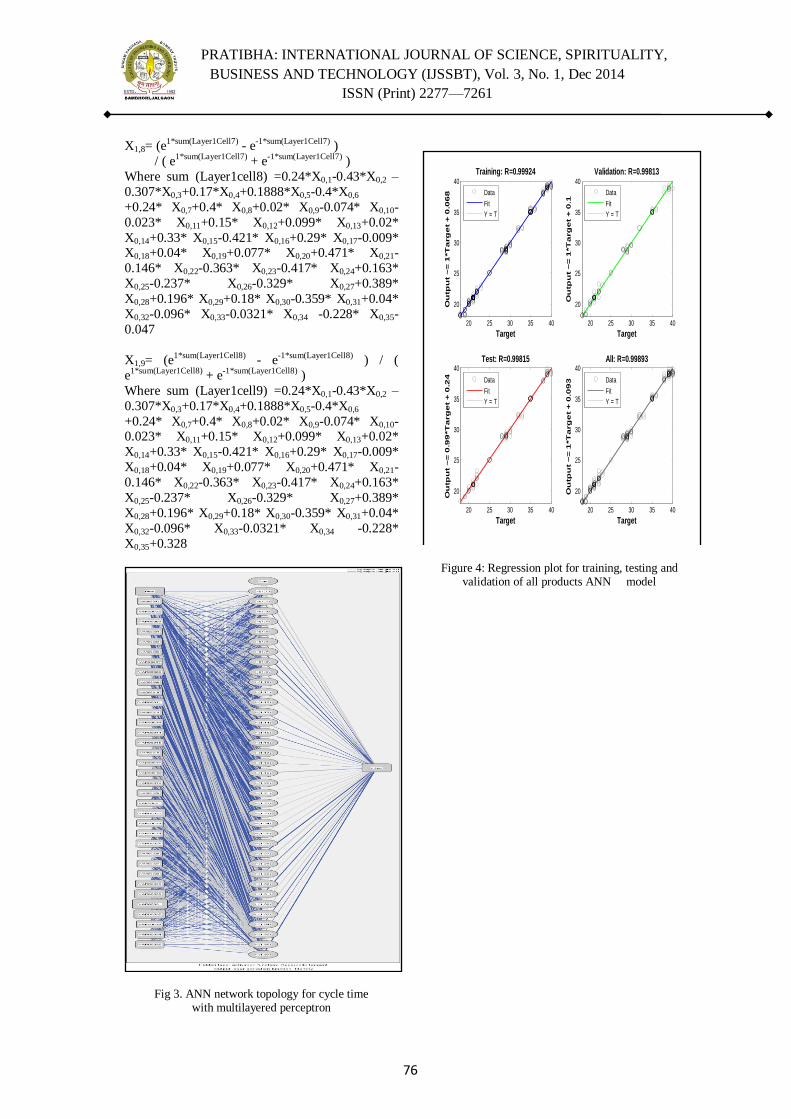
PRATIBHA: INTERNATIONAL JOURNAL OF SCIENCE, SPIRITUALITY,
BUSINESS AND TECHNOLOGY (IJSSBT), Vol. 3, No. 1, Dec 2014
ISSN (Print) 2277—7261
76
X1,8= (e1*sum(Layer1Cell7) - e-1*sum(Layer1Cell7) )
/ ( e1*sum(Layer1Cell7)
+ e-1*sum(Layer1Cell7)
)
Where sum (Layer1cell8) =0.24*X0,1-0.43*X0,2 –
0.307*X0,3+0.17*X0,4+0.1888*X0,5-0.4*X0,6
+0.24* X0,7+0.4* X0,8+0.02* X0,9-0.074* X0,10-
0.023* X0,11+0.15* X0,12+0.099* X0,13+0.02*
X0,14+0.33* X0,15-0.421* X0,16+0.29* X0,17-0.009* X0,18+0.04* X0,19+0.077* X0,20+0.471* X0,21-
0.146* X0,22-0.363* X0,23-0.417* X0,24+0.163*
X0,25-0.237* X0,26-0.329* X0,27+0.389*
X0,28+0.196* X0,29+0.18* X0,30-0.359* X0,31+0.04*
X0,32-0.096* X0,33-0.0321* X0,34 -0.228* X0,35-
0.047
X1,9= (e1*sum(Layer1Cell8) - e-1*sum(Layer1Cell8) ) / (
e1*sum(Layer1Cell8) + e-1*sum(Layer1Cell8) )
Where sum (Layer1cell9) =0.24*X0,1-0.43*X0,2 –
0.307*X0,3+0.17*X0,4+0.1888*X0,5-0.4*X0,6
+0.24* X0,7+0.4* X0,8+0.02* X0,9-0.074* X0,10-0.023* X0,11+0.15* X0,12+0.099* X0,13+0.02*
X0,14+0.33* X0,15-0.421* X0,16+0.29* X0,17-0.009*
X0,18+0.04* X0,19+0.077* X0,20+0.471* X0,21-
0.146* X0,22-0.363* X0,23-0.417* X0,24+0.163*
X0,25-0.237* X0,26-0.329* X0,27+0.389*
X0,28+0.196* X0,29+0.18* X0,30-0.359* X0,31+0.04*
X0,32-0.096* X0,33-0.0321* X0,34 -0.228*
X0,35+0.328
Fig 3. ANN network topology for cycle time with multilayered perceptron
Figure 4: Regression plot for training, testing and validation of all products ANN model
20 25 30 35 40
20
25
30
35
40
Target
Ou
tpu
t ~
= 1
*T
arg
et
+ 0
.06
8
Training: R=0.99924
Data
Fit
Y = T
20 25 30 35 40
20
25
30
35
40
Target
Ou
tpu
t ~
= 1
*T
arg
et
+ 0
.1
Validation: R=0.99813
Data
Fit
Y = T
20 25 30 35 40
20
25
30
35
40
Target
Ou
tpu
t ~
= 0
.99
*T
arg
et
+ 0
.24
Test: R=0.99815
Data
Fit
Y = T
20 25 30 35 40
20
25
30
35
40
Target
Ou
tpu
t ~
= 1
*T
arg
et
+ 0
.09
3
All: R=0.99893
Data
Fit
Y = T
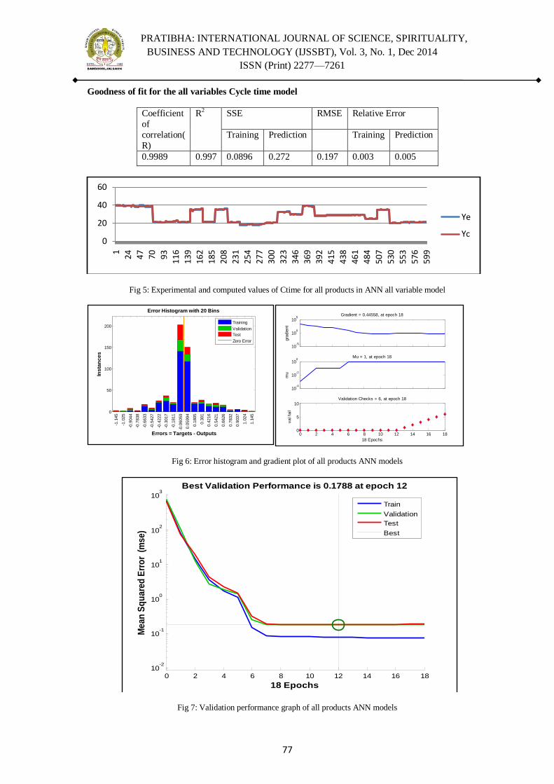
PRATIBHA: INTERNATIONAL JOURNAL OF SCIENCE, SPIRITUALITY,
BUSINESS AND TECHNOLOGY (IJSSBT), Vol. 3, No. 1, Dec 2014
ISSN (Print) 2277—7261
77
Goodness of fit for the all variables Cycle time model
Coefficient
of
correlation(
R)
R2 SSE RMSE Relative Error
Training Prediction Training Prediction
0.9989 0.997 0.0896 0.272 0.197 0.003 0.005
Fig 5: Experimental and computed values of Ctime for all products in ANN all variable model
Fig 6: Error histogram and gradient plot of all products ANN models
Fig 7: Validation performance graph of all products ANN models
0
20
40
60
1
24 47 70 93 11
6
13
9
16
2
18
5
20
8
23
1
25
4
27
7
30
0
32
3
34
6
36
9
39
2
41
5
43
8
46
1
48
4
50
7
53
0
55
3
57
6
59
9
Ye
Yc
0
50
100
150
200
Error Histogram with 20 Bins
Ins
tan
ce
s
Errors = Targets - Outputs
-1.1
45
-1.0
25
-0.9
044
-0.7
838
-0.6
633
-0.5
427
-0.4
222
-0.3
017
-0.1
811
-0.0
6059
0.0
5994
0.1
805
0.3
01
0.4
216
0.5
421
0.6
626
0.7
832
0.9
037
1.0
24
1.1
45
Training
Validation
Test
Zero Error
10-5
100
105
gra
die
nt
Gradient = 0.44558, at epoch 18
10-4
10-2
100
mu
Mu = 1, at epoch 18
0 2 4 6 8 10 12 14 16 180
5
10
val fa
il
18 Epochs
Validation Checks = 6, at epoch 18
0 2 4 6 8 10 12 14 16 1810
-2
10-1
100
101
102
103
Best Validation Performance is 0.1788 at epoch 12
Me
an
Sq
ua
red
Err
or
(m
se
)
18 Epochs
Train
Validation
Test
Best
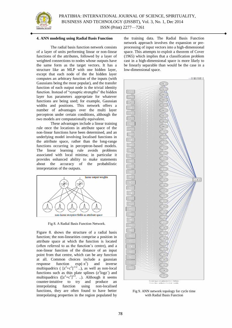
PRATIBHA: INTERNATIONAL JOURNAL OF SCIENCE, SPIRITUALITY,
BUSINESS AND TECHNOLOGY (IJSSBT), Vol. 3, No. 1, Dec 2014
ISSN (Print) 2277—7261
78
4. ANN modeling using Radial Basis Function
The radial basis function network consists
of a layer of units performing linear or non-linear
functions of the attributes, followed by a layer of
weighted connections to nodes whose outputs have
the same form as the target vectors. It has a
structure like an MLP with one hidden layer, except that each node of the the hidden layer
computes an arbitrary function of the inputs (with
Gaussians being the most popular), and the transfer
function of each output node is the trivial identity
function. Instead of ―synaptic strengths‖ the hidden
layer has parameters appropriate for whatever
functions are being used; for example, Gaussian
widths and positions. This network offers a
number of advantages over the multi layer
perceptron under certain conditions, although the
two models are computationally equivalent.
These advantages include a linear training rule once the locations in attribute space of the
non-linear functions have been determined, and an
underlying model involving localised functions in
the attribute space, rather than the long-range
functions occurring in perceptron-based models.
The linear learning rule avoids problems
associated with local minima; in particular it
provides enhanced ability to make statements
about the accuracy of the probabilistic
interpretation of the outputs.
Fig 8. A Radial Basis Function Network.
Figure 8. shows the structure of a radial basis
function; the non-linearities comprise a position in
attribute space at which the function is located
(often referred to as the function‘s centre), and a
non-linear function of the distance of an input
point from that centre, which can be any function
at all. Common choices include a gaussian
response function exp(-x2) and inverse
multiquadrics ( [z2+c2]-1/2 ..), as well as non-local
functions such as thin plate splines (z2logz¨) and
multiquadrics ([z2+c2]1/2. ..). Although it seems counter-intuitive to try and produce an
interpolating function using non-localised
functions, they are often found to have better
interpolating properties in the region populated by
the training data. The Radial Basis Function
network approach involves the expansion or pre-
processing of input vectors into a high-dimensional
space. This attempts to exploit a theorem of Cover
(1965) which implies that a classification problem
cast in a high-dimensional space is more likely to
be linearly separable than would be the case in a
low-dimensional space.
Fig 9. ANN network topology for cycle time with Radial Basis Function
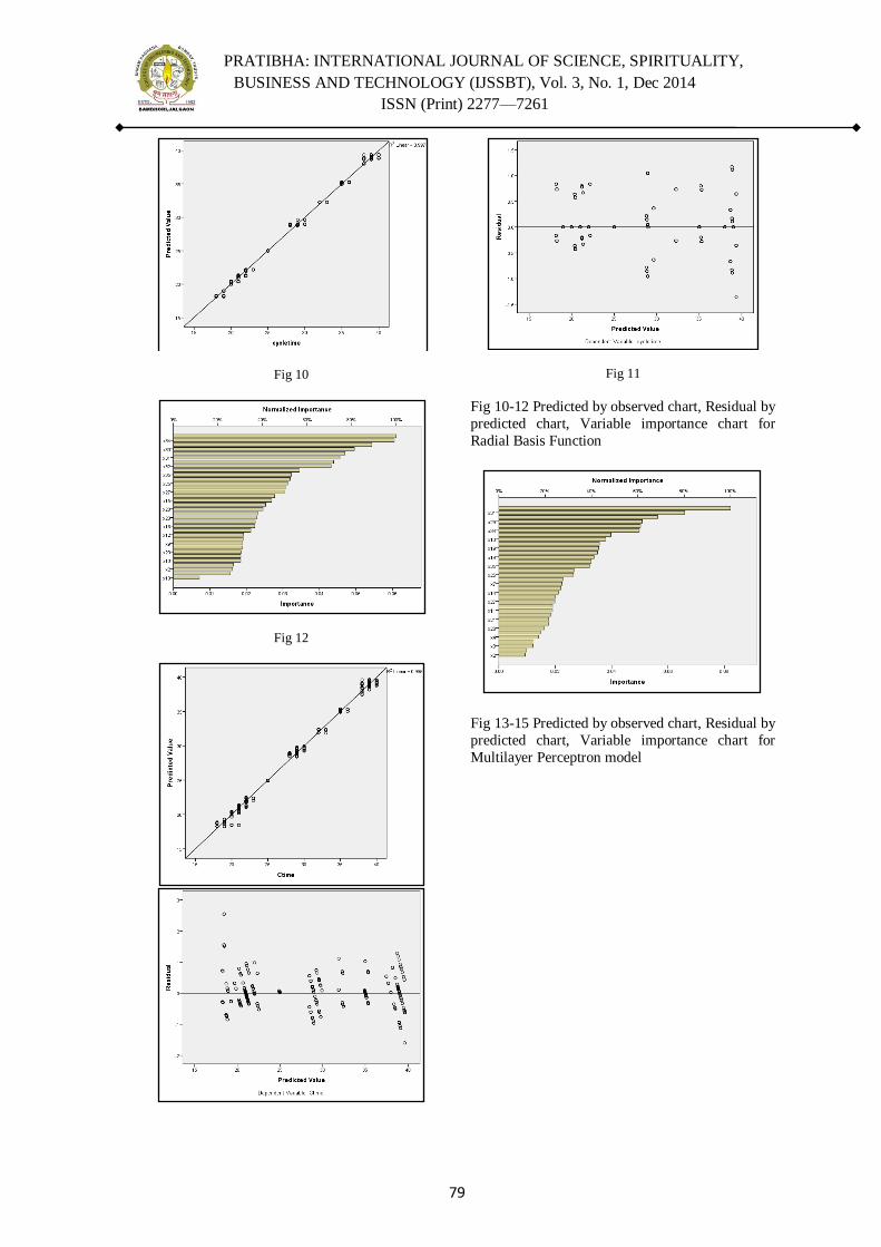
PRATIBHA: INTERNATIONAL JOURNAL OF SCIENCE, SPIRITUALITY,
BUSINESS AND TECHNOLOGY (IJSSBT), Vol. 3, No. 1, Dec 2014
ISSN (Print) 2277—7261
79
Fig 10
Fig 12
Fig 11
Fig 10-12 Predicted by observed chart, Residual by
predicted chart, Variable importance chart for
Radial Basis Function
Fig 13-15 Predicted by observed chart, Residual by
predicted chart, Variable importance chart for
Multilayer Perceptron model

PRATIBHA: INTERNATIONAL JOURNAL OF SCIENCE, SPIRITUALITY,
BUSINESS AND TECHNOLOGY (IJSSBT), Vol. 3, No. 1, Dec 2014
ISSN (Print) 2277—7261
80
5. Result and Discussion
Table 1: Performance of Radial Basis Neural Network
ANN
Network Topology
R R2 Relative Error Sum of Square Error
Training Testing Training Testing
35-10-1 0.613 0.376 0.608 0.663 122.248 60.033
35-15-1 0.794 0.631 0.333 0.476 71.230 36.780
35-20-1 0.879 0.773 0.194 0.299 39.394 27.685
35-25-1 0.948 0.899 0.108 0.088 22.328 8.804
35-30-1 0.985 0.971 0.008 0.078 1.688 6.905
35-31-1 0.994 0.990 0.010 0.011 2.053 0.957
35-32-1 0.994 0.990 0.007 0.018 1.372 1.635
35-33-1 0.994 0.990 0.008 0.015 1.638 1.312
35-34-1 0.988 0.977 0.004 0.073 0.888 6.040
35-35-1 0.982 0.996 0.004 0.361 0.785 0.361
35-36-1 0.982 0.996 0.004 0.004 0.848 0.374
35-37-1 0.998 0.997 0.003 0.003 0.637 0.288
Table 2: Performance of Multilayer Perceptron Neural Network
ANN Network Topology
R R2 Relative Error Sum of Square Error
Training Testing Training Testing
35-10-1 0.998 0.997 0.003 0.004 0.247 0.169
35-15-1 0.998 0.997 0.003 0.004 0.245 0.129
35-20-1 0.993 0.988 0.017 0.017 1.435 0.670
35-25-1 0.997 0.996 0.004 0.005 0.320 0.202
35-30-1 0.998 0.997 0.003 0.003 0.228 0.115
35-31-1 0.996 0.993 0.007 0.007 0.656 0.244
35-32-1 0.998 0.997 0.002 0.003 0.217 0.129
35-33-1 0.997 0.995 0.004 0.006 0.367 0.208
35-34-1 0.998 0.997 0.003 0.004 0.269 0.122
35-35-1 0.997 0.996 0.004 0.005 0.369 0.166
35-36-1 0.998 0.997 0.003 0.003 0.265 0.125
35-37-1 0.997 0.995 0.004 0.005 0.405 0.171

PRATIBHA: INTERNATIONAL JOURNAL OF SCIENCE, SPIRITUALITY,
BUSINESS AND TECHNOLOGY (IJSSBT), Vol. 3, No. 1, Dec 2014
ISSN (Print) 2277—7261
81
Data from field process generated array is
considered as a input for neural network modeling
.Two diversified approach of Multilayered
perceptron and Radial basis function is used to fit
neural network model .The corresponding transfer
function used for Radial basis function model is
softmax on the contrary transfer function for Multilayered perceptron model is hyperbolic
tangential function for input layer and hyperbolic
tan for output layer.
The topologies which envisaged for ANN
model generation are implemented purely on trial
and error basis. Started with by default 10 number
of hidden neurons in hidden layer number 1 to
maximum 37 hidden nodes in hidden layer have
been tried . Radial basis function yielded with low
coefficient of correlation at early stage of function
fitting with 10 hidden nodes with relatively large
SSE (122.248, 60.033) for training and testing samples. Though relative error doesn‘t shows large
difference which indicated that the network is not
overstrain. Radial basis function performs well
with 37 hidden nodes with very minimum SSE as
well as relative error.
Multilayered Perceptron network
performs relatively well even with 10 hidden nodes
.Overall range of SSE and relative error is
predominantly well placed in multilayered
perceptron model. It fits well with topologies of
35-10-1, 35-15-1, 35-30-1, 35-34-1, 35-37-1. Coefficient of correlation is well closed to 1 which
indicated that multilayered perceptron is able to
predict cycle time better than anticipation.
6. Conclusion:
This paper ultimately exhibits the
comparison of two distinct function fitting
processes of Neural network. The overall results
reflects that multilayered perceptron outperformed
Radial Basis function in terms of stability of network as well as constant performs even with
minimum number of hidden nodes. The range of
SSE for Radial basis function 0.228 to 122.248 is
on higher side compare to Multilayered perceptron.
With range of coefficient of correlation (0.993-
0.998), multilayered perceptron would be the
obvious choice for prediction of cycle time under
defined set of conditions.
7. References
[1] Timothy James Stich, Dr. Julie K. Spoerre & Dr. Tomas
Velasco, 2000. ―The Application of Artificial Neural
Networks to Monitoring and Control of an Induction
Hardening Process‖. Journal of Industrial Technology
Volume 16, National Association of Industrial
Technology.
[2] Fan, H. T., and Wu, S. M., 1995, Case studies on
modeling manufacturing processes using artificial neural
networks.Journal of Engineering for Industry, 117, 412-
417.
[3] Smith, A. E., & Mason, A. K. 1997. ―Cost estimation
predictive modeling: Regression versus neural network.‖
The Engineering Economist, 42 (2), 137–161
[4] John D. Dowler, 2008 ―Using Neural Networks with
Limited Data to Estimate Manufacturing Cost‖ .Master of
Science theses, The Russ College of Engineering and
Technology of Ohio University
[5] Bishop, C. M. 1995. Neural Networks for Pattern
Recognition, 3rd ed. Oxford: Oxford University Press.
[6] Fine, T. L. 1999. Feedforward Neural Network
Methodology, 3rd ed. New York: Springer-Verlag.
[7] Haykin, S. 1998. Neural Networks: A Comprehensive
Foundation, 2nd ed. New York: Macmillan College
Publishing.
[8] Ripley, B. D. 1996. Pattern Recognition and Neural
Networks. Cambridge: Cambridge University Press.
[9] Smith, A. E., & Mason, A. K. 1997. ―Cost estimation
predictive modeling: Regression versus neural
network.‖The Engineering Economist, 42 (2), 137–161
[10] Swingler, K. 1996. ―Applying Neural Networks A
practical guide.‖ Morgan Kaufmann.
[11] Walpole, Myers, Myers, and Ye. 2002. ―Probability &
Statistics for engineers & scientists‖7thedition, Prentice
Hall
[12] Fine, Terrence. 1999. ―Feedforward Neural Network
Methodology (Springer Series in Statistics)‖ 1 edition,
Springer
[13] [13] Marco Garetti, Marco Taisch, 2010. ―Neural
networks in production planning and Control‖. Production
planning & control , 1999, vol. 10, no. 4, 324
[14] Frans Vainio,Mika Johnsson,Michael Maier,Timo
Knuutila ,Olli S. Nevalainen ,Esa Alhoniemi
,2009.―Estimating printed circuit board assembly times
using neural networks‖. International Journal of
production Research, 48:8, 2201-2218
[15] Fine T. (1999), Feedforward Neural Network
Methodology; Springer Series in Statistics; 1st edition,
Springer.
[16] Günaydin, H. Murat, Dogan, S. Zeynep. (2004), A neural
network approach for early cost estimation of structural
systems of buildings; International Journal of Project
Management 22; 595-602.
[17] Seo K.K., Park J.H., Jang D.S., Wallace D. (2002),
Approximate estimation of the product life cycle cost
using neural networks in conceptual design; International
Journal of Advanced Manufacturing Technology 19; 461-
471.
[18] Curry, B., Morgan, P., & Silver, M. (2002). Neural
networks and non-linear statistical methods: An
application to the modeling or price-quality relationships.
Computers and Operations Research, 29, 951–969.
[19] DeTienne, K. B., DeTienne, D. H., & Joshi, S. A. (2003).
Neural networks as statistical tools for business
researchers. Organizational Research Methods, 6(2), 236–
265.
[20] Ozel, T. and Karpat, Y., 2005. Predictive modelling of
surface roughness and tool wear in hard turning using
regression and neural networks. International Journal of
Machine Tools and Manufacture, 45 (4–5), 467–479.
[21] Cook, D. F., and Chiu, C. C., Using radial basis function
neural networks to recognize shift in correlated
manufacturing process parameters, IIE Transactions, 30,
227, 1998
[22] Baillie, D. and J. Mathew. (1994) Diagnosing Rolling
Element Bearing Faults with Artificial Neural Networks.
Acoustics Australia, 22(3), 79-84.

PRATIBHA: INTERNATIONAL JOURNAL OF SCIENCE, SPIRITUALITY,
BUSINESS AND TECHNOLOGY (IJSSBT), Vol. 3, No. 1, Dec 2014
ISSN (Print) 2277—7261
82
[23] Meesad, P. and G.G. Yen. (2000) Pattern classification by
a neurofuzzy network: application to vibration
monitoring. ISA Transactions, 39(3), 293-308.
[24] McCormick, A.C. and A.K. Nandi.(1996), ―A comparison
of artificial neural networks and other statistical methods
for rotating machine condition classification‖, IEE
Colloquium on Modelling and Signal Processing for Fault
Diagnosis UK (Ref. No.1996/260). Pp. 100.
[25] IEE London UK.
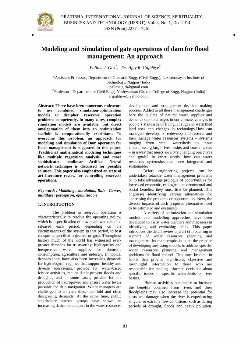
PRATIBHA: INTERNATIONAL JOURNAL OF SCIENCE, SPIRITUALITY,
BUSINESS AND TECHNOLOGY (IJSSBT), Vol. 3, No. 1, Dec 2014
ISSN (Print) 2277—7261
83
Modeling and Simulation of gate operations of dam for flood
management: An approach
Pallavi J. Giri*, Dr. Ajay R. Gajbhiye
#
*Assistant Professor, Department of Genearal Engg. (Civil Engg.), Laxminarayan Institute of
Technology, Nagpur (India)
[email protected] # Professor, Department of Civil Engg. Yeshwantrao Chavan College of Engg, Nagpur (India)
Abstract: There have been numerous endeavors
to use combined simulation-optimization
models to decipher reservoir operation
problems competently. In many cases, complex
simulation models are available, but direct
amalgamation of them into an optimization
scaffold is computationally exorbitant. To
overcome this problem, an approach for
modeling and simulation of Dam operation for
flood management is suggested in this paper.
Traditional mathematical modeling techniques
like multiple regression analysis and more
sophisticated nonlinear Artifical Neural
network technique is discussed for possible
solution .This paper also emphasized on state of
art literature review for controlling reservoir
operations.
Key words : Modeling , simulation, Rule - Curves,
multilayer perceptron, optimization
1. INTRODUCTION
The problem in reservoir operation is
characteristically to resolve the operating policy,
which is a specification of how much water is to be
released each period, depending on the
circumstances of the system in that period, to best conquer a specified objective or goal. Throughout
history much of the world has witnessed ever-
greater demands for trustworthy, high-quality and
inexpensive water supplies for domestic
consumption, agriculture and industry. In topical
decades there have also been increasing demands
for hydrological regimes that support healthy and
diverse ecosystems, provide for water-based
leisure activities, reduce if not prevent floods and
droughts, and in some cases, provide for the
production of hydropower and ensure water levels
passable for ship navigation. Water managers are challenged to convene these manifold and often
disagreeing demands. At the same time, public
stakeholder interest groups have shown an
increasing desire to take part in the water resources
development and management decision making
process. Added to all these management challenges
bare the qualms of natural water supplies and demands due to changes in our climate, changes in
people‘s standards of living, changes in watershed
land uses and changes in technology.How can
managers develop, or redevelop and restore, and
then manage water resources systems – systems
ranging from small watersheds to those
encompassing large river basins and coastal zones
– in a way that meets society‘s changing objectives
and goals? In other words, how can water
resources systemsbecome more integrated and
sustainable?
Before engineering projects can be undertaken totackle water management problems
or to take advantage prologue of opportunities for
increased economic, ecological, environmental and
social benefits, they must first be planned. This
engrosses identifying various alternatives for
addressing the problems or opportunities. Next, the
diverse impacts of each proposed alternative need
to be estimated and evaluated.
A variety of optimization and simulation
models and modelling approaches have been
developed to assist water planners and managers in identifying and evaluating plans. This paper
introduces the detail review and art of modelling in
support of water resources planning and
management. Its main emphasis is on the practice
of developing and using models to address specific
water resources planning and management
problems for flood control. This must be done in
habits that provide significant, objective and
meaningful information to those who are
responsible for making informed decisions about
specific issues in specific watersheds or river basins.
Human activities commence to increase
the benefits obtained from rivers and their
floodplains may also increase the potential for
costs and damage when the river is experiencing
singular or extreme flow conditions, such as during
periods of drought, floods and heavy pollution.
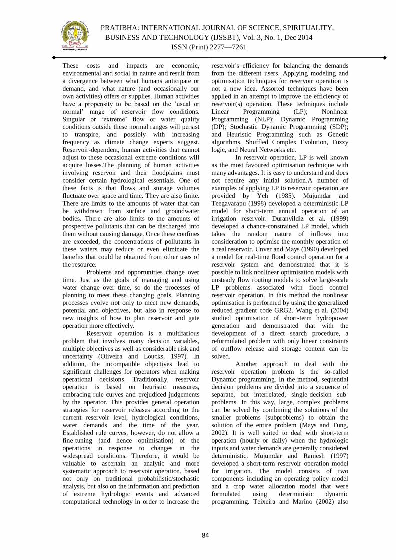
PRATIBHA: INTERNATIONAL JOURNAL OF SCIENCE, SPIRITUALITY,
BUSINESS AND TECHNOLOGY (IJSSBT), Vol. 3, No. 1, Dec 2014
ISSN (Print) 2277—7261
84
These costs and impacts are economic,
environmental and social in nature and result from
a divergence between what humans anticipate or
demand, and what nature (and occasionally our
own activities) offers or supplies. Human activities
have a propensity to be based on the ‗usual or
normal‘ range of reservoir flow conditions.
Singular or ‗extreme‘ flow or water quality conditions outside these normal ranges will persist
to transpire, and possibly with increasing
frequency as climate change experts suggest.
Reservoir-dependent, human activities that cannot
adjust to these occasional extreme conditions will
acquire losses.The planning of human activities
involving reservoir and their floodplains must
consider certain hydrological essentials. One of
these facts is that flows and storage volumes
fluctuate over space and time. They are also finite.
There are limits to the amounts of water that can
be withdrawn from surface and groundwater bodies. There are also limits to the amounts of
prospective pollutants that can be discharged into
them without causing damage. Once these confines
are exceeded, the concentrations of pollutants in
these waters may reduce or even eliminate the
benefits that could be obtained from other uses of
the resource.
Problems and opportunities change over
time. Just as the goals of managing and using
water change over time, so do the processes of
planning to meet these changing goals. Planning processes evolve not only to meet new demands,
potential and objectives, but also in response to
new insights of how to plan reservoir and gate
operation more effectively.
Reservoir operation is a multifarious
problem that involves many decision variables,
multiple objectives as well as considerable risk and
uncertainty (Oliveira and Loucks, 1997). In
addition, the incompatible objectives lead to
significant challenges for operators when making
operational decisions. Traditionally, reservoir operation is based on heuristic measures,
embracing rule curves and prejudiced judgements
by the operator. This provides general operation
strategies for reservoir releases according to the
current reservoir level, hydrological conditions,
water demands and the time of the year.
Established rule curves, however, do not allow a
fine-tuning (and hence optimisation) of the
operations in response to changes in the
widespread conditions. Therefore, it would be
valuable to ascertain an analytic and more
systematic approach to reservoir operation, based not only on traditional probabilistic/stochastic
analysis, but also on the information and prediction
of extreme hydrologic events and advanced
computational technology in order to increase the
reservoir's efficiency for balancing the demands
from the different users. Applying modeling and
optimisation techniques for reservoir operation is
not a new idea. Assorted techniques have been
applied in an attempt to improve the efficiency of
reservoir(s) operation. These techniques include
Linear Programming (LP); Nonlinear
Programming (NLP); Dynamic Programming (DP); Stochastic Dynamic Programming (SDP);
and Heuristic Programming such as Genetic
algorithms, Shuffled Complex Evolution, Fuzzy
logic, and Neural Networks etc.
In reservoir operation, LP is well known
as the most favoured optimisation technique with
many advantages. It is easy to understand and does
not require any initial solution.A number of
examples of applying LP to reservoir operation are
provided by Yeh (1985). Mujumdar and
Teegavarapu (1998) developed a deterministic LP
model for short-term annual operation of an irrigation reservoir. Duranyildiz et al. (1999)
developed a chance-constrained LP model, which
takes the random nature of inflows into
consideration to optimise the monthly operation of
a real reservoir. Unver and Mays (1990) developed
a model for real-time flood control operation for a
reservoir system and demonstrated that it is
possible to link nonlinear optimisation models with
unsteady flow routing models to solve large-scale
LP problems associated with flood control
reservoir operation. In this method the nonlinear optimisation is performed by using the generalized
reduced gradient code GRG2. Wang et al. (2004)
studied optimisation of short-term hydropower
generation and demonstrated that with the
development of a direct search procedure, a
reformulated problem with only linear constraints
of outflow release and storage content can be
solved.
Another approach to deal with the
reservoir operation problem is the so-called
Dynamic programming. In the method, sequential decision problems are divided into a sequence of
separate, but interrelated, single-decision sub-
problems. In this way, large, complex problems
can be solved by combining the solutions of the
smaller problems (subproblems) to obtain the
solution of the entire problem (Mays and Tung,
2002). It is well suited to deal with short-term
operation (hourly or daily) when the hydrologic
inputs and water demands are generally considered
deterministic. Mujumdar and Ramesh (1997)
developed a short-term reservoir operation model
for irrigation. The model consists of two components including an operating policy model
and a crop water allocation model that were
formulated using deterministic dynamic
programming. Teixeira and Marino (2002) also
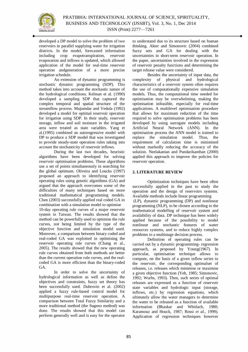
PRATIBHA: INTERNATIONAL JOURNAL OF SCIENCE, SPIRITUALITY,
BUSINESS AND TECHNOLOGY (IJSSBT), Vol. 3, No. 1, Dec 2014
ISSN (Print) 2277—7261
85
developed a DP model to solve the problem of two
reservoirs in parallel supplying water for irrigation
districts. In the model, forecasted information
including crop evapotranspiration, reservoir
evaporation and inflows is updated, which allowed
application of the model for real-time reservoir
operation andgeneration of a more precise
irrigation schedule. An extension of dynamic programming is
stochastic dynamic programming (SDP). This
method takes into account the stochastic nature of
the hydrological conditions. Kelman et al. (1990)
developed a sampling SDP that captured the
complex temporal and spatial structure of the
streamflow process. Mujumdar and Vedula (1992)
developed a model for optimal reservoir operation
for irrigation using SDP. In their study, reservoir
storage, inflow and soil moisture in the irrigated
area were treated as state variables. Yang et
al.(1995) combined an autoregressive model with DP to produce a SDP model that was investigated
to provide steady-state operation rules taking into
account the stochasticity of reservoir inflows.
During the last two decades, heuristic
algorithms have been developed for solving
reservoir optimisation problems. These algorithms
use a set of points simultaneously in searching for
the global optimum. Oliveira and Loucks (1997)
proposed an approach to identifying reservoir
operating rules using genetic algorithms (GA) and
argued that the approach overcomes some of the difficulties of many techniques based on more
traditional mathematical programming models.
Chen (2003) successfully applied real coded GA in
combination with a simulation model to optimise
10-day operating rule curves of a major reservoir
system in Taiwan. The results showed that the
method can be powerfully used to optimise the rule
curves, not being limited by the type of the
objective function and simulation model used.
Moreover, a comparison between binary coded and
real-coded GA was exploited in optimising the reservoir operating rule curves (Chang et al.,
2005). The results showed that the new operating
rule curves obtained from both methods are better
than the current operation rule curves, and the real-
coded GA is more efficient than the binary-coded
GA.
In order to solve the uncertainty of
hydrological information as well as define the
objectives and constraints, fuzzy set theory has
been successfully used. Dubrovin et al. (2002)
applied a fuzzy rule-based control model for
multipurpose real-time reservoir operation. A comparison between Total Fuzzy Similarity and a
more traditional method (the Sugeno method) was
done. The results showed that this model can
perform generally well and is easy for the operator
to understand due to its structure based on human
thinking. Akter and Simonovic (2004) combined
fuzzy sets and GA for dealing with the
uncertainties in short-term reservoir operation. In
the paper, uncertainties involved in the expression
of reservoir penalty functions and determining the
target release value were considered.
Besides the uncertainty of input data, the complexity of physical and hydrological
characteristics of a reservoir system often requires
the use of computationally expensive simulation
models. Thus, the computational time needed for
optimisation may be overwhelming, making the
optimisation infeasible, especially for real-time
applications. A multilevel optimisation procedure
that allows for maximum reduction of the time
required to solve optimisation problems has been
developed by using surrogate models including
Artificial Neural Network (ANN). In the
optimisation process the ANN model is trained to replace the simulation model. Thus, the
requirement of calculation time is minimised
without markedly reducing the accuracy of the
solution. Neelakantan and Pundarikanthan (2000)
applied this approach to improve the policies for
reservoir operation.
2. LITERATURE REVIEW
Optimization techniques have been often
successfully applied in the past to study the
operation and the design of reservoirs systems.
Available methods include linear programming
(LP), dynamic programming (DP) and nonlinear
programming (NLP), to be chosen according to the
mathematical modelling of reservoir system and
availability of data. DP technique has been widely
applied because of the possibility to model nonlinear and stochastic features of water
resources systems, and to reduce highly complex
problems to a multistage decision process.
Definition of operating rules can be
carried out by a dynamic programming- regression
approach, as proposed by Young(1967). In
particular, optimisation technique allows to
compute, on the basis of a given inflow series to
the reservoir, the corresponding optimalset of
releases, i.e. releases which minimise or maximise
a given objective function (Yeh, 1985; Simonovic, 1992; Wurbs, 1993). Then, such series of optimal
releases are expressed as a function of reservoir
state variables and hydrologic input (storage,
inflows, etc.) by regression equations, which
ultimately allow the water managers to determine
the water to be released as a function of available
information (Bhaskar and Whitlach, 1980;
Karamouz and Houck, 1987; Rossi et al., 1999).
Application of regression techniques however
PRATIBHA: INTERNATIONAL JOURNAL OF SCIENCE, SPIRITUALITY,
BUSINESS AND TECHNOLOGY (IJSSBT), Vol. 3, No. 1, Dec 2014
ISSN (Print) 2277—7261
86
requires the explicit definition of the link between
independent and dependent variables. To partly
overcome such difficulty, a new interpolation
method based on Neural Networks (NN) has been
recently applied in several fields of research; it can
also be considered as a candidate technique to the
determination of operating rules. NN are able to
approximate a wide range of multivariate linear and non-linear functions, while maintaining very
good generalisation capabilities, and therefore they
are ideal candidates if the relationship among the
variables is unknown. They have been applied for
interpretation, prediction, diagnosis, planning,
monitoring, debugging, repair, instruction, and
control, but the most successful applications are in
categorization and pattern recognition; in fact, they
have been shown to perform successfully where
other methods do not, recognizing and matching
complicated, vague, or incomplete patterns.
Young (1967) derived operating rules using simple linear regression or multiple linear
regression from the deterministic optimization
results. He derived regression equations using
inflows and storages to find optimal releases.
Bhaskar and Whitlach (1980) analyzed a single
multipurpose reservoir using backward DP
algorithm to obtain optimal results. Bhaskar and
Whitlach (1980) made use of the procedure of
deriving general operating policies from
deterministic optimization as initiated by Young
(1967). Bhaskar and Whitlach (1980) considered a quadratic loss function and derived monthly
policies by regressing optimal set of releases on
the input and state variables. They concluded that
for two-sided quadratic loss functions performance
of linear policies were better than nonlinear
policies and for one-sided quadratic loss functions
nonlinear policies gave improved performance.
Karamouz and Houck (1982) developed reservoir
system operating rules by deterministic
optimization using the DPR model. The DPR
model algorithm had a deterministic dynamic program with a regression analysis. This algorithm
also had a simulation model to assess the
performance. A hypothetical loss function was
used which involved only reservoir release. By
considering the recommendations of Bhaskar and
Whitlach (1980), Karamouz and Houck (1982)
analyzed the DPR model performance with case
studies, and suggested that the model can be
extended easily to more complex and more
practical problems. Wurbs et al. (1985) presented
an annotated bibliography for various optimization
and simulation models and listed several applications made by various researchers in the
reservoir operation problems using LP, DP, NLP,
and simulation models. Karamouz and Houck
(1987) further compared deterministic DP and
regression-based DPR model with stochastic DP
(SDP) model. The deterministic DPR model and
the SDP model were formulated with the same
objective function. As a continuing effort,
Karamouz et al. (1992) used an implicit stochastic
optimization scheme for multiple reservoir
systems. The optimal operations from the
deterministic optimization were then analyzed in a regression procedure to obtain a set of operating
rules as they did in the single reservoir case. These
rules were evaluated using a simulation model and
a different set of data. Wurbs (1993) reviewed the
reservoir system simulation and optimization
models. This review was done with the objective to
contribute to ongoing efforts throughout the water
management community in sorting through the
numerous reservoir system-analysis models.
Simonovic (1992) presented a short review of
mathematical models used in reservoir
management and operation. This review was intended to present conclusions reached by
previous state-of-the-art reviews and to provide
ideas for closing the gap between theory and
practice. Simonovic (1992) presented a simple
simulation-optimization model for reservoir sizing
and showed how it responded to practical needs of
water resources engineers. Yang and Read (1999)
developed a constructive DP which is successfully
applied to optimize releases in a stochastic two-
reservoir model of the New Zealand power system.
Takyi and Lence (1999) developed a surface water quality management model using a multiple-
realization chance constraint method for more
complex systems.
In last years NN have found more and
more application in hydraulics and hydrologic
field, and also in water management studies.
Among the recent state-of-arts on the subject the
following are worth to be mentioned. The first part
of a study published in ASCE (2000a) focused on
setting a conceptual framework for the application
of NN to related hydrologic issues, by comparing the modelling capabilities of NN with other
traditional modelling approaches. Applications of
NN to many nonlinear hydrologic processes such
as rainfall-runoff modelling, streamflow
forecasting, ground water, precipitation
forecasting, and water quality issues, can be found
in the second part of the ASCE study (ASCE,
2000b), as well as in Govindaraju and
Ramachandra(2000). NN have showed a great
potential in prediction problems, although a good
understanding of the underlying physical processes
seemed to be a key factor for successful applications. The study also pointed out the need
for further investigations, to be conducted when
applying NN, about the choice of their
architecture, the optimal training data set, etc. In
PRATIBHA: INTERNATIONAL JOURNAL OF SCIENCE, SPIRITUALITY,
BUSINESS AND TECHNOLOGY (IJSSBT), Vol. 3, No. 1, Dec 2014
ISSN (Print) 2277—7261
87
water management, NN have been applied for
deriving reservoir operating policies with reference
to different types of water supply systems. Raman
and Chandramouli (1996) trained neural network
by backpropagation algorithm based on a
supervised learning for deriving operating rules
from optimization results. The suggested model
algorithm had three important modules. First was a deterministic optimization algorithm with an
objective function to minimize the squared deficit.
The results of the DP optimization were printed in
a file. The results were treated as training patterns.
These training patterns were used to train the
neural network. The second module was a neural
network with back-propagation algorithm to train
the network, and the third module had a reservoir-
simulation algorithm that could be used to study
the performance. The performance of the DPN
model was compared with the SDP model—an
explicit stochastic model constructed with the same objective function. Further, the model was
compared with standard operating policy which is
being practiced in the field. Neelakantan and
Pundarikanthan (1999) applied a simulation-
optimisation procedure to improve the operation of
a municipal water supply reservoir under deficit
conditions. The operation policies were based on a
hedging rule, able to avoid extreme deficit
conditions and to increase the system
sustainability. In order to speed up the
optimization process, NN were used to replace traditional models in the reservoirs system
simulation. This allowed for a more efficient
screening of the potential operation policies. Rossi
et al. (1999) compared the linear regression
approach vs the neural network approach, for
deriving operating rules of a reservoir supplying an
irrigation district. Monthly optimal releases were
obtained by DP, assuming the sum of square
deficits as objective function. Reservoir storage at
the beginning of the current month, streamflow
and release during the previous month were selected as independent variables. Results
indicated that NN performed better than multiple
linear regression.
Jain et al. (1999) applied NN for two
different tasks. First, NN were used for predicting
inflows to a reservoir part of a multipurpose
project devoted primarily to irrigation and
generation of electric power. Then reservoir
operation policies were formulated relating optimal
releases with storage, inflow and demand trough
linear and nonlinear regressions and NN.
Cancelliere et al. (2000) analyzed the effects of the presence of severe drought years in the definition
of the operating rules of an irrigation reservoir
through the use of DP and NN techniques. The
selected rules were compared on the basis of
reservoir performance indices and crop yield
losses. Chandramouli and Raman (2001) made an
attempt to extend the DP-NN model, previously
applied to a single reservoir, to a multireservoir
project. A DP formulation of three reservoirs
working in conjunction was developed, and
operating rules were derived using regression
models and NN. French et al. (1992) developed three-layered NN to forecast rainfall intensity
fields in space and time. After training with input
patterns, the NN was used to forecast rainfall using
the current fields as input. French et al. (1992)
showed that NN was capable of learning the
complex relationship describing the space-time
evolution of rainfall. Ranjithan et al. (1993) used
neural network-based screening approach for
ground-water reclamation. Saad et al. (1994)
described a disaggregation procedure by training
an NN. After training, this network gave the
storage level of each reservoir of a system when supplied with the value of an aggregate storage
level. The training set was obtained by solving the
deterministic operation problem of a large number
of equally likely flow sequences. Saad et al. (1994)
used back-propagation algorithm and the
minimization of quadratic error was computed by
gradient method. The aggregated storage level was
determined by SDP algorithm in which all
hydroelectric reservoirs were aggregated to form
one equivalent reservoir. Saad et al. (1994)
presented a comparison with principal component-analysis disaggregation technique with NN-based
technique. Smith and Eli (1995) used ANN to
model rainfall runoff process. They used a 5 3 5
grid cell synthetic watershed to generate runoff
from stochastically generated rainfall patterns.
Smith and Eli (1995) used a backpropagation
algorithm for training to predict the peak discharge
and the time of peak resulting from single rainfall
pattern. Muller (1996) and Babovic and Larsen
(1998) reported many applications of decision
support and management systems, geographic information systems, and neural networks. Hsu et
al. (1999) used artificial neural network for the
estimation of physical variables from multichannel
remotely sensed imageries for rainfall estimation.
In neural network approach a successfully trained
network tries to capture the interrelationship
between the trained data sets which closely
approximate the target values. The application of
NNs in water resources showed their usefulness
and many applications are reported in literature.
Many successful applications of fuzzy
systems were reported in the literature, especially in control and modeling - Fontane et al. 1997;
Dubrovin et al. (2002). They are suitable for
situations where an exact model of a process is
either impractical or very costly to build, but an

PRATIBHA: INTERNATIONAL JOURNAL OF SCIENCE, SPIRITUALITY,
BUSINESS AND TECHNOLOGY (IJSSBT), Vol. 3, No. 1, Dec 2014
ISSN (Print) 2277—7261
88
imprecise model based on the existing human
expertise can do the job. In such situations, fuzzy
systems are considered as the best alternative,
though they do not perform optimally. Fuzzy sets
are an aid in providing information in a more
human comprehensible or natural form, and can
handle uncertainties at various levels. The
knowledge contained in fuzzy systems is transparent to the user. On the other hand, artificial
neural networks ANNs are also used successfully
for single reservoir as well as Multireservoir
operation Raman and Chandramouli 1996; Jain et
al. 1999; Chandramouli and Raman 2001. While
neural networks are ideal for modeling known or
unknown associations that exist between the input
and output data, significant data cleaning and
preprocessing are usually needed. In other words,
input data must be carefully prepared for the
network to process. The more input data, the better
the training results. The richer the input data, then more accurate is the model. However, training
requires substantial time and resources. These
difficulties restrict the widespread use of neural
networks in many applications - Badiru and
Cheung (2002). In many decision-making systems,
it is important to be able to explain the process by
which the decision is made. The concepts of fuzzy
logic clearly compliment those of neural networks.
While fuzzy logic provides simple data
representation, neural networks provide none.
Where fuzzy logic can be used to model a system, neural networks are well suited to provide
sophisticated models of diverse type of systems.
However, if there is prior knowledge about the
underlying system, fuzzy logic can readily
encapsulate the knowledge in terms of rules and
relations, while it is not particularly easy to
preprogram a neural network with prior
knowledge. Given a set of training samples, it is
not simple to train a fuzzy model, but many
algorithms have been developed in the past for
training neural networks. The concept of neurofuzzy hybrid systems has emerged as
researchers have tried to combine the transparent,
linguistic representation of a fuzzy system with the
learning ability of an ANN Brown and Harris
(1994). A neurofuzzy system uses an ANN
learning algorithm to determine its parameters i.e.,
fuzzy sets and fuzzy rules_ by processing data
samples. Therefore, it can be trained to perform an
input-output mapping, just as with an ANN, but
with the additional benefit of being able to provide
the set of rules on which the model is based. Deka
and Chandramouli (2003) developed a fuzzy neural network model for deriving river stage-
discharge relationship at selected gauging stations
of Brahmaputra River in India and found better
than other models considered.
Deka and Chandramouli (2005) also
found that fuzzy neural network modeling used in
routing river flow was better than other models
considered. Chaves and Kojiri (2007) developed a
conceptual fuzzy neural network(CFNN) for water
quality simulation in Barra Bonita reservoir system
in Brazil using a genetic algorithm as the training
method for finding fuzzy inference and connection weights. They found that the CFNN model showed
greater robustness and reliability while dealing
with systems for which data are considered to be
vague, uncertain, or incomplete.
According to the World Commission on
Dams, many large storage projects worldwide are
failing to produce the anticipated benefits
(Labadie, 2004). Similarly, small storage projects
made for local areas in developing countries, like
India, are also failing to meet expectations. The
main cause identified at various levels of
discussion, as reported by Labadie (2004), is inadequate consideration of the more mundane
operation and maintenance issues once the project
is completed. For existing reservoirs, optimum
operation is critical, since all the expected benefits
are based on timely water releases to meet the
stipulated demand. Real-time operation of a
reservoir requires making relatively quick
decisions regarding releases based on short-term
information. Decisions are dependent on the
storage in the reservoir and information available
in the form of forecast hydrologic and meteorological parameters. This is especially
important duringfloods and power generation,
where the system has to respond to changes very
quickly and may need to adapt rapidly (Mohan et
al., 1991). For reservoir systems operated for
irrigation scheduling, real-time operation is not
very common because of longer decision steps.
Traditionally, the reservoirs meant for irrigation
purposes are operated on heuristics and certain
rules derived from previous experiences. This
defies search capability and near global optimal values. It originated in the mid 1970s (Holland,
1975) and emerged as a powerful optimization
approach. An excellent introduction to Genetic
Algorithm (GA) is given by Goldberg (1989), and
several recent researchers have summarised the
essentials of genetic algorithm modelling (Deb,
1995; Wang, 1991; Oliveira and Loucks, 1997;
Wardlaw and Sharif, 1999)(Fig. 1). The
application of GA to ground water problems
(Ritzel et al., 1994; Aly and Peralta, 1999; Reed et
al., 2003; Hilton and Culver, 2005; Espinoza et al.
2005), and water distribution network problems (Dandy and Engelhardt, 2001;Wu and Simpson,
2001) has been studied extensively. The
application of GA to reservoir operation problems
began in the last decade of the 21st century. East
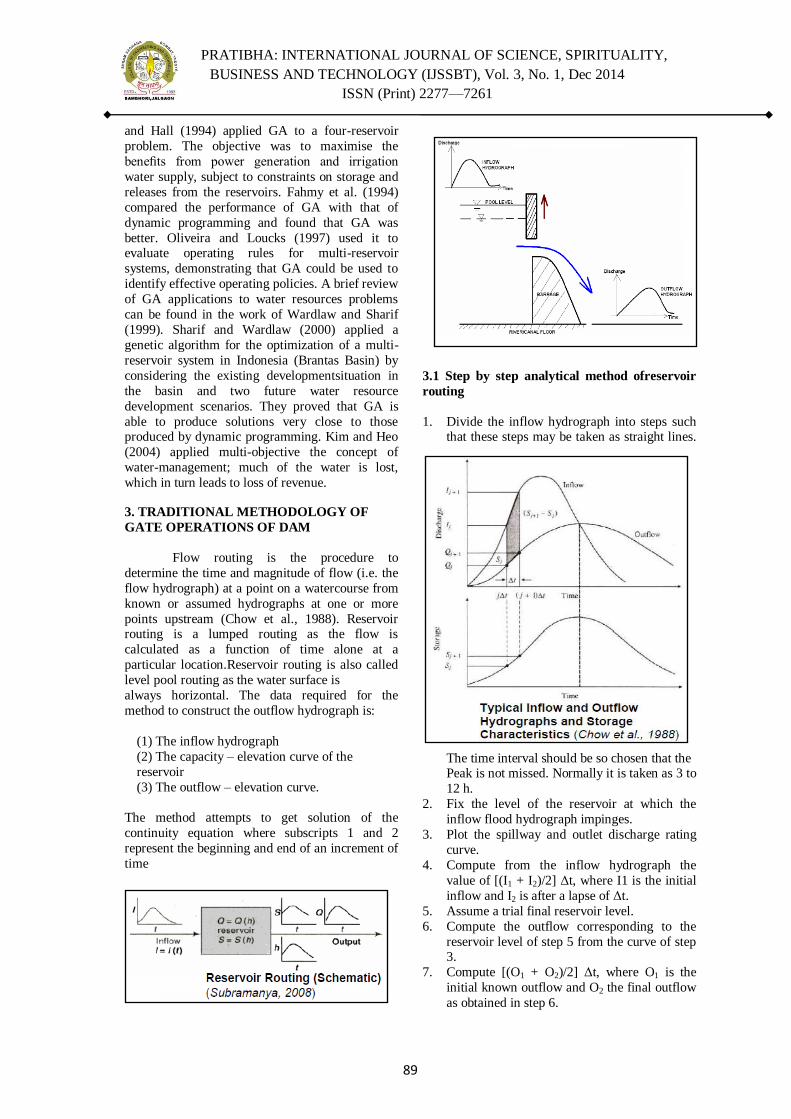
PRATIBHA: INTERNATIONAL JOURNAL OF SCIENCE, SPIRITUALITY,
BUSINESS AND TECHNOLOGY (IJSSBT), Vol. 3, No. 1, Dec 2014
ISSN (Print) 2277—7261
89
and Hall (1994) applied GA to a four-reservoir
problem. The objective was to maximise the
benefits from power generation and irrigation
water supply, subject to constraints on storage and
releases from the reservoirs. Fahmy et al. (1994)
compared the performance of GA with that of
dynamic programming and found that GA was
better. Oliveira and Loucks (1997) used it to evaluate operating rules for multi-reservoir
systems, demonstrating that GA could be used to
identify effective operating policies. A brief review
of GA applications to water resources problems
can be found in the work of Wardlaw and Sharif
(1999). Sharif and Wardlaw (2000) applied a
genetic algorithm for the optimization of a multi-
reservoir system in Indonesia (Brantas Basin) by
considering the existing developmentsituation in
the basin and two future water resource
development scenarios. They proved that GA is
able to produce solutions very close to those produced by dynamic programming. Kim and Heo
(2004) applied multi-objective the concept of
water-management; much of the water is lost,
which in turn leads to loss of revenue.
3. TRADITIONAL METHODOLOGY OF
GATE OPERATIONS OF DAM
Flow routing is the procedure to
determine the time and magnitude of flow (i.e. the
flow hydrograph) at a point on a watercourse from
known or assumed hydrographs at one or more
points upstream (Chow et al., 1988). Reservoir routing is a lumped routing as the flow is
calculated as a function of time alone at a
particular location.Reservoir routing is also called
level pool routing as the water surface is
always horizontal. The data required for the
method to construct the outflow hydrograph is:
(1) The inflow hydrograph
(2) The capacity – elevation curve of the
reservoir
(3) The outflow – elevation curve.
The method attempts to get solution of the
continuity equation where subscripts 1 and 2
represent the beginning and end of an increment of
time
3.1 Step by step analytical method ofreservoir
routing
1. Divide the inflow hydrograph into steps such that these steps may be taken as straight lines.
The time interval should be so chosen that the Peak is not missed. Normally it is taken as 3 to
12 h.
2. Fix the level of the reservoir at which the
inflow flood hydrograph impinges.
3. Plot the spillway and outlet discharge rating
curve.
4. Compute from the inflow hydrograph the
value of [(I1 + I2)/2] Δt, where I1 is the initial
inflow and I2 is after a lapse of Δt.
5. Assume a trial final reservoir level.
6. Compute the outflow corresponding to the
reservoir level of step 5 from the curve of step 3.
7. Compute [(O1 + O2)/2] Δt, where O1 is the
initial known outflow and O2 the final outflow
as obtained in step 6.
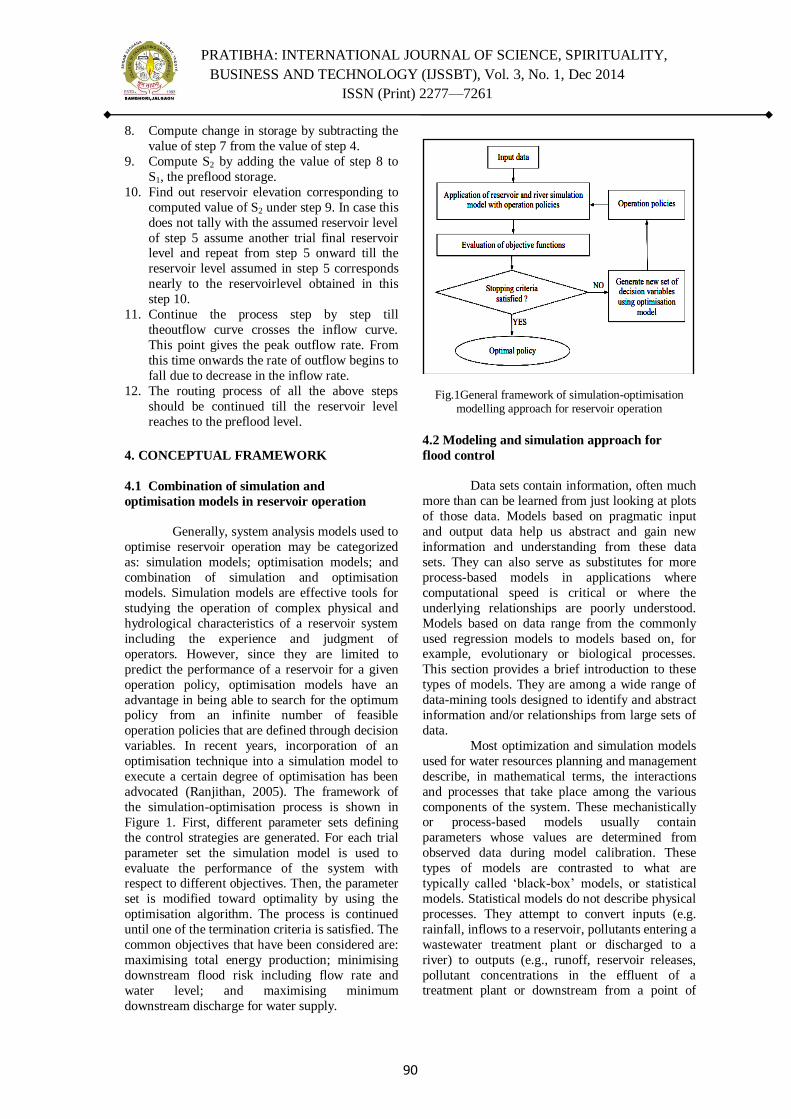
PRATIBHA: INTERNATIONAL JOURNAL OF SCIENCE, SPIRITUALITY,
BUSINESS AND TECHNOLOGY (IJSSBT), Vol. 3, No. 1, Dec 2014
ISSN (Print) 2277—7261
90
8. Compute change in storage by subtracting the
value of step 7 from the value of step 4.
9. Compute S2 by adding the value of step 8 to
S1, the preflood storage.
10. Find out reservoir elevation corresponding to
computed value of S2 under step 9. In case this
does not tally with the assumed reservoir level
of step 5 assume another trial final reservoir level and repeat from step 5 onward till the
reservoir level assumed in step 5 corresponds
nearly to the reservoirlevel obtained in this
step 10.
11. Continue the process step by step till
theoutflow curve crosses the inflow curve.
This point gives the peak outflow rate. From
this time onwards the rate of outflow begins to
fall due to decrease in the inflow rate.
12. The routing process of all the above steps
should be continued till the reservoir level
reaches to the preflood level.
4. CONCEPTUAL FRAMEWORK
4.1 Combination of simulation and
optimisation models in reservoir operation
Generally, system analysis models used to
optimise reservoir operation may be categorized
as: simulation models; optimisation models; and
combination of simulation and optimisation
models. Simulation models are effective tools for
studying the operation of complex physical and
hydrological characteristics of a reservoir system
including the experience and judgment of
operators. However, since they are limited to
predict the performance of a reservoir for a given
operation policy, optimisation models have an
advantage in being able to search for the optimum policy from an infinite number of feasible
operation policies that are defined through decision
variables. In recent years, incorporation of an
optimisation technique into a simulation model to
execute a certain degree of optimisation has been
advocated (Ranjithan, 2005). The framework of
the simulation-optimisation process is shown in
Figure 1. First, different parameter sets defining
the control strategies are generated. For each trial
parameter set the simulation model is used to
evaluate the performance of the system with respect to different objectives. Then, the parameter
set is modified toward optimality by using the
optimisation algorithm. The process is continued
until one of the termination criteria is satisfied. The
common objectives that have been considered are:
maximising total energy production; minimising
downstream flood risk including flow rate and
water level; and maximising minimum
downstream discharge for water supply.
Fig.1General framework of simulation-optimisation modelling approach for reservoir operation
4.2 Modeling and simulation approach for
flood control
Data sets contain information, often much
more than can be learned from just looking at plots
of those data. Models based on pragmatic input
and output data help us abstract and gain new
information and understanding from these data
sets. They can also serve as substitutes for more
process-based models in applications where
computational speed is critical or where the
underlying relationships are poorly understood.
Models based on data range from the commonly
used regression models to models based on, for example, evolutionary or biological processes.
This section provides a brief introduction to these
types of models. They are among a wide range of
data-mining tools designed to identify and abstract
information and/or relationships from large sets of
data.
Most optimization and simulation models
used for water resources planning and management
describe, in mathematical terms, the interactions
and processes that take place among the various
components of the system. These mechanistically or process-based models usually contain
parameters whose values are determined from
observed data during model calibration. These
types of models are contrasted to what are
typically called ‗black-box‘ models, or statistical
models. Statistical models do not describe physical
processes. They attempt to convert inputs (e.g.
rainfall, inflows to a reservoir, pollutants entering a
wastewater treatment plant or discharged to a
river) to outputs (e.g., runoff, reservoir releases,
pollutant concentrations in the effluent of a treatment plant or downstream from a point of
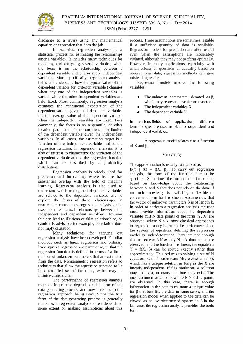
PRATIBHA: INTERNATIONAL JOURNAL OF SCIENCE, SPIRITUALITY,
BUSINESS AND TECHNOLOGY (IJSSBT), Vol. 3, No. 1, Dec 2014
ISSN (Print) 2277—7261
91
discharge to a river) using any mathematical
equation or expression that does the job.
In statistics, regression analysis is a
statistical process for estimating the relationships
among variables. It includes many techniques for
modeling and analyzing several variables, when
the focus is on the relationship between a
dependent variable and one or more independent variables. More specifically, regression analysis
helps one understand how the typical value of the
dependent variable (or 'criterion variable') changes
when any one of the independent variables is
varied, while the other independent variables are
held fixed. Most commonly, regression analysis
estimates the conditional expectation of the
dependent variable given the independent variables
i.e. the average value of the dependent variable
when the independent variables are fixed. Less
commonly, the focus is on a quantile, or other
location parameter of the conditional distribution of the dependent variable given the independent
variables. In all cases, the estimation target is a
function of the independent variables called the
regression function. In regression analysis, it is
also of interest to characterize the variation of the
dependent variable around the regression function
which can be described by a probability
distribution.
Regression analysis is widely used for
prediction and forecasting, where its use has
substantial overlap with the field of machine learning. Regression analysis is also used to
understand which among the independent variables
are related to the dependent variable, and to
explore the forms of these relationships. In
restricted circumstances, regression analysis can be
used to infer causal relationships between the
independent and dependent variables. However
this can lead to illusions or false relationships, so
caution is advisable for example, correlation does
not imply causation.
Many techniques for carrying out regression analysis have been developed. Familiar
methods such as linear regression and ordinary
least squares regression are parametric, in that the
regression function is defined in terms of a finite
number of unknown parameters that are estimated
from the data. Nonparametric regression refers to
techniques that allow the regression function to lie
in a specified set of functions, which may be
infinite-dimensional.
The performance of regression analysis
methods in practice depends on the form of the
data generating process, and how it relates to the regression approach being used. Since the true
form of the data-generating process is generally
not known, regression analysis often depends to
some extent on making assumptions about this
process. These assumptions are sometimes testable
if a sufficient quantity of data is available.
Regression models for prediction are often useful
even when the assumptions are moderately
violated, although they may not perform optimally.
However, in many applications, especially with
small effects or questions of causality based on
observational data, regression methods can give misleading results.
Regression models involve the following
variables:
The unknown parameters, denoted as β,
which may represent a scalar or a vector. The independent variables X.
The dependent variable Y.
In various fields of application, different
terminologies are used in place of dependent and independent variables.
A regression model relates Y to a function
of X and β.
Y≈ f (X, β)
The approximation is usually formalized as
E(Y | X) = f(X, β). To carry out regression analysis, the form of the function f must be
specified. Sometimes the form of this function is
based on knowledge about the relationship
between Y and X that does not rely on the data. If
no such knowledge is available, a flexible or
convenient form for f is chosen.Assume now that
the vector of unknown parameters β is of length k.
In order to perform a regression analysis the user
must provide information about the dependent
variable Y:If N data points of the form (Y, X) are
observed, where N < k, most classical approaches
to regression analysis cannot be performed: since the system of equations defining the regression
model is underdetermined, there are not enough
data to recover β.If exactly N = k data points are
observed, and the function f is linear, the equations
Y = f(X, β) can be solved exactly rather than
approximately. This reduces to solving a set of N
equations with N unknowns (the elements of β),
which has a unique solution as long as the X are
linearly independent. If f is nonlinear, a solution
may not exist, or many solutions may exist. The
most common situation is where N > k data points are observed. In this case, there is enough
information in the data to estimate a unique value
for β that best fits the data in some sense, and the
regression model when applied to the data can be
viewed as an overdetermined system in β.In the
last case, the regression analysis provides the tools
for:
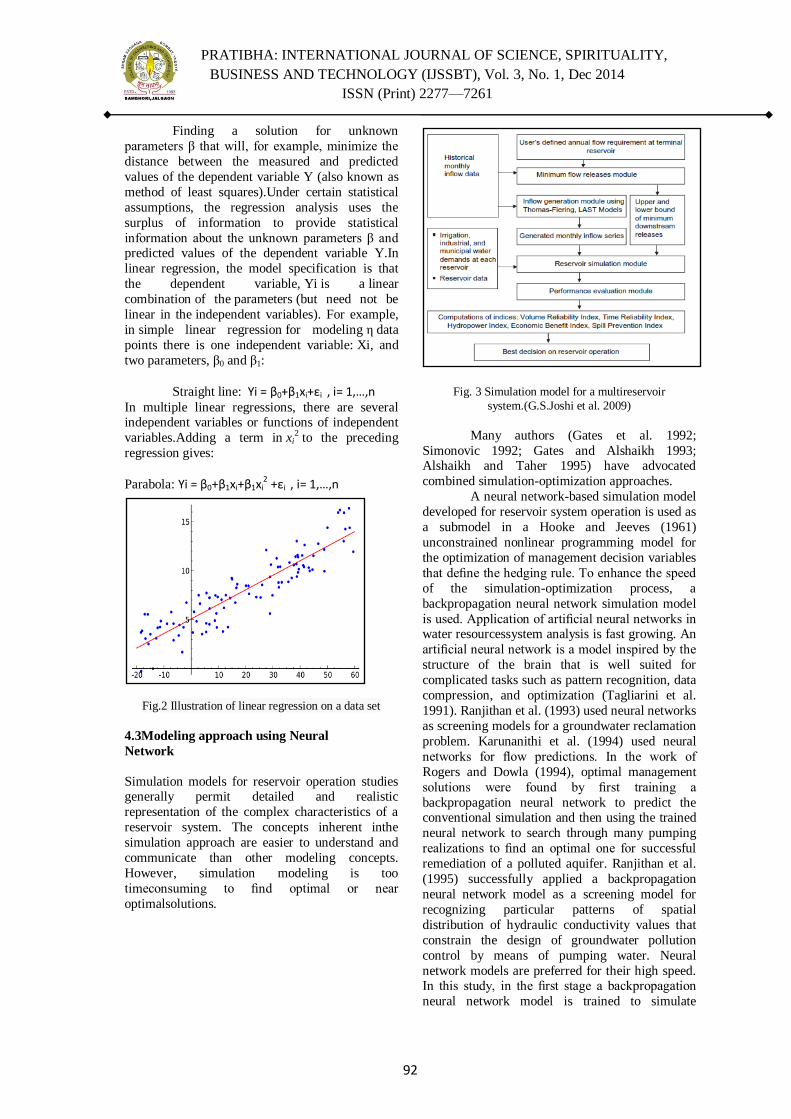
PRATIBHA: INTERNATIONAL JOURNAL OF SCIENCE, SPIRITUALITY,
BUSINESS AND TECHNOLOGY (IJSSBT), Vol. 3, No. 1, Dec 2014
ISSN (Print) 2277—7261
92
Finding a solution for unknown
parameters β that will, for example, minimize the
distance between the measured and predicted
values of the dependent variable Y (also known as
method of least squares).Under certain statistical
assumptions, the regression analysis uses the
surplus of information to provide statistical
information about the unknown parameters β and predicted values of the dependent variable Y.In
linear regression, the model specification is that
the dependent variable, Yi is a linear
combination of the parameters (but need not be
linear in the independent variables). For example,
in simple linear regression for modeling η data
points there is one independent variable: Xi, and
two parameters, β0 and β1:
Straight line: Yi = β0+β1xi+εi , i= 1,…,n
In multiple linear regressions, there are several independent variables or functions of independent
variables.Adding a term in xi2 to the preceding
regression gives:
Parabola: Yi = β0+β1xi+β1xi2 +εi , i= 1,…,n
Fig.2 Illustration of linear regression on a data set
4.3Modeling approach using Neural
Network
Simulation models for reservoir operation studies generally permit detailed and realistic
representation of the complex characteristics of a
reservoir system. The concepts inherent inthe
simulation approach are easier to understand and
communicate than other modeling concepts.
However, simulation modeling is too
timeconsuming to find optimal or near
optimalsolutions.
Fig. 3 Simulation model for a multireservoir
system.(G.S.Joshi et al. 2009)
Many authors (Gates et al. 1992;
Simonovic 1992; Gates and Alshaikh 1993; Alshaikh and Taher 1995) have advocated
combined simulation-optimization approaches.
A neural network-based simulation model
developed for reservoir system operation is used as
a submodel in a Hooke and Jeeves (1961)
unconstrained nonlinear programming model for
the optimization of management decision variables
that define the hedging rule. To enhance the speed
of the simulation-optimization process, a
backpropagation neural network simulation model
is used. Application of artificial neural networks in water resourcessystem analysis is fast growing. An
artificial neural network is a model inspired by the
structure of the brain that is well suited for
complicated tasks such as pattern recognition, data
compression, and optimization (Tagliarini et al.
1991). Ranjithan et al. (1993) used neural networks
as screening models for a groundwater reclamation
problem. Karunanithi et al. (1994) used neural
networks for flow predictions. In the work of
Rogers and Dowla (1994), optimal management
solutions were found by first training a
backpropagation neural network to predict the conventional simulation and then using the trained
neural network to search through many pumping
realizations to find an optimal one for successful
remediation of a polluted aquifer. Ranjithan et al.
(1995) successfully applied a backpropagation
neural network model as a screening model for
recognizing particular patterns of spatial
distribution of hydraulic conductivity values that
constrain the design of groundwater pollution
control by means of pumping water. Neural
network models are preferred for their high speed. In this study, in the first stage a backpropagation
neural network model is trained to simulate
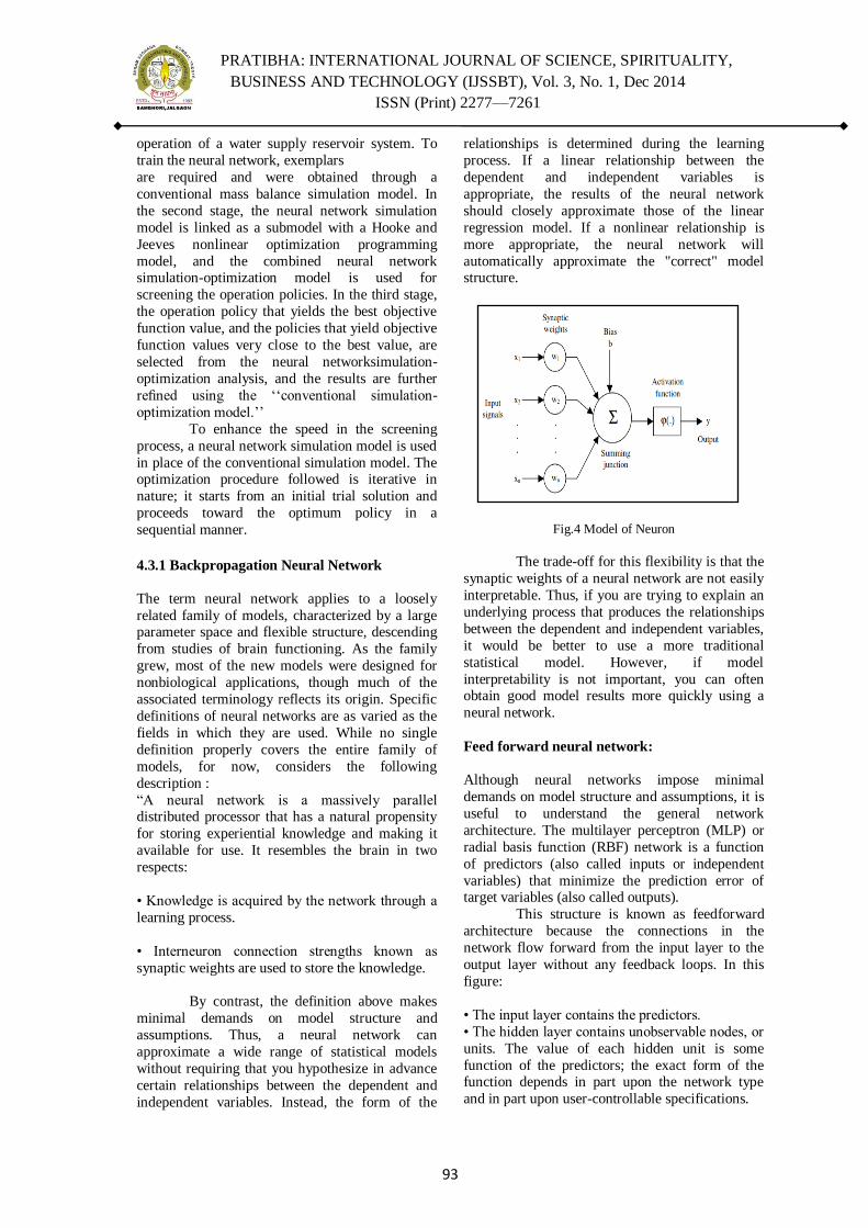
PRATIBHA: INTERNATIONAL JOURNAL OF SCIENCE, SPIRITUALITY,
BUSINESS AND TECHNOLOGY (IJSSBT), Vol. 3, No. 1, Dec 2014
ISSN (Print) 2277—7261
93
operation of a water supply reservoir system. To
train the neural network, exemplars
are required and were obtained through a
conventional mass balance simulation model. In
the second stage, the neural network simulation
model is linked as a submodel with a Hooke and
Jeeves nonlinear optimization programming
model, and the combined neural network simulation-optimization model is used for
screening the operation policies. In the third stage,
the operation policy that yields the best objective
function value, and the policies that yield objective
function values very close to the best value, are
selected from the neural networksimulation-
optimization analysis, and the results are further
refined using the ‗‗conventional simulation-
optimization model.‘‘
To enhance the speed in the screening
process, a neural network simulation model is used
in place of the conventional simulation model. The optimization procedure followed is iterative in
nature; it starts from an initial trial solution and
proceeds toward the optimum policy in a
sequential manner.
4.3.1 Backpropagation Neural Network
The term neural network applies to a loosely
related family of models, characterized by a large parameter space and flexible structure, descending
from studies of brain functioning. As the family
grew, most of the new models were designed for
nonbiological applications, though much of the
associated terminology reflects its origin. Specific
definitions of neural networks are as varied as the
fields in which they are used. While no single
definition properly covers the entire family of
models, for now, considers the following
description :
―A neural network is a massively parallel distributed processor that has a natural propensity
for storing experiential knowledge and making it
available for use. It resembles the brain in two
respects:
• Knowledge is acquired by the network through a
learning process.
• Interneuron connection strengths known as
synaptic weights are used to store the knowledge.
By contrast, the definition above makes
minimal demands on model structure and
assumptions. Thus, a neural network can
approximate a wide range of statistical models
without requiring that you hypothesize in advance
certain relationships between the dependent and
independent variables. Instead, the form of the
relationships is determined during the learning
process. If a linear relationship between the
dependent and independent variables is
appropriate, the results of the neural network
should closely approximate those of the linear
regression model. If a nonlinear relationship is
more appropriate, the neural network will
automatically approximate the "correct" model structure.
Fig.4 Model of Neuron
The trade-off for this flexibility is that the
synaptic weights of a neural network are not easily
interpretable. Thus, if you are trying to explain an
underlying process that produces the relationships
between the dependent and independent variables,
it would be better to use a more traditional
statistical model. However, if model
interpretability is not important, you can often obtain good model results more quickly using a
neural network.
Feed forward neural network:
Although neural networks impose minimal
demands on model structure and assumptions, it is
useful to understand the general network
architecture. The multilayer perceptron (MLP) or
radial basis function (RBF) network is a function
of predictors (also called inputs or independent
variables) that minimize the prediction error of target variables (also called outputs).
This structure is known as feedforward
architecture because the connections in the
network flow forward from the input layer to the
output layer without any feedback loops. In this
figure:
• The input layer contains the predictors.
• The hidden layer contains unobservable nodes, or
units. The value of each hidden unit is some
function of the predictors; the exact form of the function depends in part upon the network type
and in part upon user-controllable specifications.
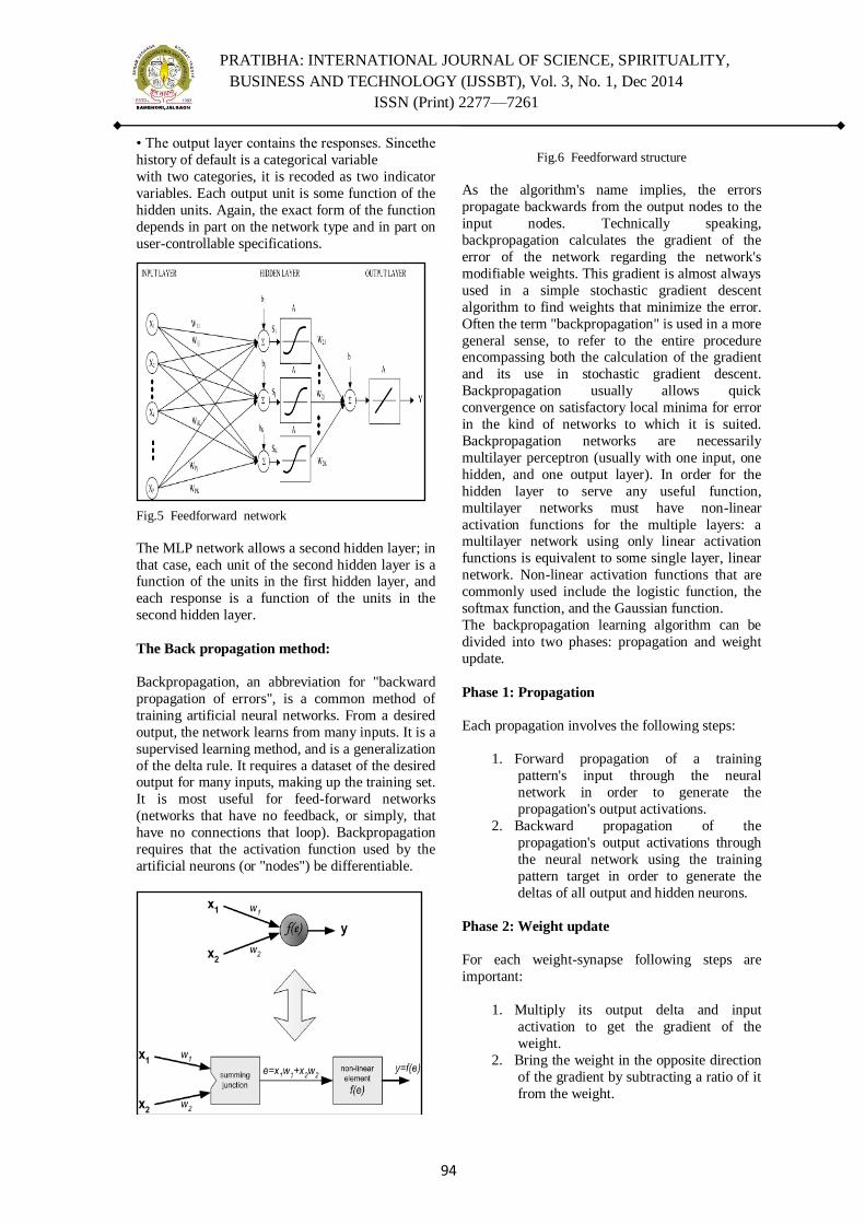
PRATIBHA: INTERNATIONAL JOURNAL OF SCIENCE, SPIRITUALITY,
BUSINESS AND TECHNOLOGY (IJSSBT), Vol. 3, No. 1, Dec 2014
ISSN (Print) 2277—7261
94
• The output layer contains the responses. Sincethe
history of default is a categorical variable
with two categories, it is recoded as two indicator
variables. Each output unit is some function of the
hidden units. Again, the exact form of the function
depends in part on the network type and in part on
user-controllable specifications.
Fig.5 Feedforward network
The MLP network allows a second hidden layer; in
that case, each unit of the second hidden layer is a function of the units in the first hidden layer, and
each response is a function of the units in the
second hidden layer.
The Back propagation method:
Backpropagation, an abbreviation for "backward
propagation of errors", is a common method of
training artificial neural networks. From a desired
output, the network learns from many inputs. It is a
supervised learning method, and is a generalization
of the delta rule. It requires a dataset of the desired output for many inputs, making up the training set.
It is most useful for feed-forward networks
(networks that have no feedback, or simply, that
have no connections that loop). Backpropagation
requires that the activation function used by the
artificial neurons (or "nodes") be differentiable.
Fig.6 Feedforward structure
As the algorithm's name implies, the errors
propagate backwards from the output nodes to the
input nodes. Technically speaking,
backpropagation calculates the gradient of the
error of the network regarding the network's
modifiable weights. This gradient is almost always
used in a simple stochastic gradient descent
algorithm to find weights that minimize the error.
Often the term "backpropagation" is used in a more
general sense, to refer to the entire procedure encompassing both the calculation of the gradient
and its use in stochastic gradient descent.
Backpropagation usually allows quick
convergence on satisfactory local minima for error
in the kind of networks to which it is suited.
Backpropagation networks are necessarily
multilayer perceptron (usually with one input, one
hidden, and one output layer). In order for the
hidden layer to serve any useful function,
multilayer networks must have non-linear
activation functions for the multiple layers: a multilayer network using only linear activation
functions is equivalent to some single layer, linear
network. Non-linear activation functions that are
commonly used include the logistic function, the
softmax function, and the Gaussian function.
The backpropagation learning algorithm can be
divided into two phases: propagation and weight
update.
Phase 1: Propagation
Each propagation involves the following steps:
1. Forward propagation of a training
pattern's input through the neural
network in order to generate the
propagation's output activations.
2. Backward propagation of the
propagation's output activations through
the neural network using the training
pattern target in order to generate the
deltas of all output and hidden neurons.
Phase 2: Weight update
For each weight-synapse following steps are
important:
1. Multiply its output delta and input
activation to get the gradient of the
weight.
2. Bring the weight in the opposite direction
of the gradient by subtracting a ratio of it
from the weight.
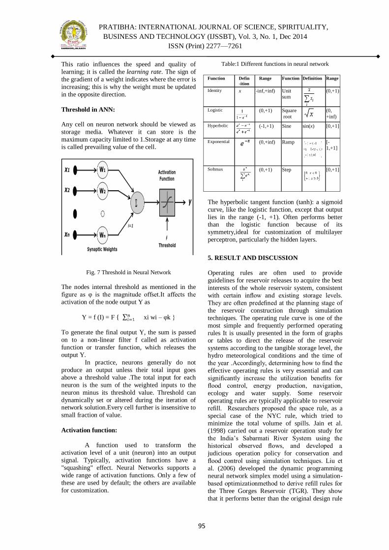
PRATIBHA: INTERNATIONAL JOURNAL OF SCIENCE, SPIRITUALITY,
BUSINESS AND TECHNOLOGY (IJSSBT), Vol. 3, No. 1, Dec 2014
ISSN (Print) 2277—7261
95
This ratio influences the speed and quality of
learning; it is called the learning rate. The sign of
the gradient of a weight indicates where the error is
increasing; this is why the weight must be updated
in the opposite direction.
Threshold in ANN:
Any cell on neuron network should be viewed as
storage media. Whatever it can store is the
maximum capacity limited to 1.Storage at any time
is called prevailing value of the cell.
Fig. 7 Threshold in Neural Network
The nodes internal threshold as mentioned in the
figure as φ is the magnitude offset.It affects the
activation of the node output Y as
Y = f (I) = F { xi wi – φk }
To generate the final output Y, the sum is passed
on to a non-linear filter f called as activation
function or transfer function, which releases the
output Y.
In practice, neurons generally do not
produce an output unless their total input goes
above a threshold value .The total input for each
neuron is the sum of the weighted inputs to the
neuron minus its threshold value. Threshold can
dynamically set or altered during the iteration of network solution.Every cell further is insensitive to
small fraction of value.
Activation function:
A function used to transform the
activation level of a unit (neuron) into an output
signal. Typically, activation functions have a
"squashing" effect. Neural Networks supports a
wide range of activation functions. Only a few of
these are used by default; the others are available
for customization.
Table:1 Different functions in neural network
Function Defin
-ition
Range Function Definition Range
Identity x (-inf,+inf) Unit
sum
(0,+1)
Logistic
(0,+1) Square
root (0,
+inf)
Hyperbolic
(-1,+1) Sine sin(x) [0,+1]
Exponential
(0,+inf) Ramp
[-
1,+1]
Softmax
(0,+1) Step
[0,+1]
The hyperbolic tangent function (tanh): a sigmoid
curve, like the logistic function, except that output
lies in the range (-1, +1). Often performs better than the logistic function because of its
symmetry,ideal for customization of multilayer
perceptron, particularly the hidden layers.
5. RESULT AND DISCUSSION
Operating rules are often used to provide
guidelines for reservoir releases to acquire the best
interests of the whole reservoir system, consistent
with certain inflow and existing storage levels.
They are often predefined at the planning stage of
the reservoir construction through simulation
techniques. The operating rule curve is one of the
most simple and frequently performed operating
rules It is usually presented in the form of graphs or tables to direct the release of the reservoir
systems according to the tangible storage level, the
hydro meteorological conditions and the time of
the year .Accordingly, determining how to find the
effective operating rules is very essential and can
significantly increase the utilization benefits for
flood control, energy production, navigation,
ecology and water supply. Some reservoir
operating rules are typically applicable to reservoir
refill. Researchers proposed the space rule, as a
special case of the NYC rule, which tried to
minimize the total volume of spills. Jain et al. (1998) carried out a reservoir operation study for
the India‘s Sabarmati River System using the
historical observed flows, and developed a
judicious operation policy for conservation and
flood control using simulation techniques. Liu et
al. (2006) developed the dynamic programming
neural network simplex model using a simulation-
based optimizationmethod to derive refill rules for
the Three Gorges Reservoir (TGR). They show
that it performs better than the original design rule

PRATIBHA: INTERNATIONAL JOURNAL OF SCIENCE, SPIRITUALITY,
BUSINESS AND TECHNOLOGY (IJSSBT), Vol. 3, No. 1, Dec 2014
ISSN (Print) 2277—7261
96
curves. Ngo et al. (2007) successfully applied the
shuffled complex evolution algorithm in
combination with the MIKE11 simulation model to
optimize the control strategies for the Hoa Binh
reservoir operation. The results show that the
method can be employed to optimize the rule
curves efficiently for reservoir operation in a multi-
objective framework. Liu et al. (2011b) proposed a multi-objective refill operation model by
combining flood control and conservation together.
Although the optimization technique can provide
an optimal rule that would maximize the economic
benefits as stipulated in many cases, its template
rule curves are derived in a fictitious way.
A gap still exists between theoretical
model development and practical operation
(Panuwat et al., 2009). Labadie (2004) pointed out
that it was difficult to make decision on operating
policies especially under uncertainty scenario due
to the randomness of natural phenomena. Many reservoir system operators feel more comfortable
to use predefined operating rules which are easy to
comprehend and operate. Therefore, important
questions are raised about how such operating
rules should be designed and managed to improve
the utilization benefits without increasing the flood
control risk for a multi-purpose reservoir. The
simulation-optimization-test framework and hybrid
multiobjective genetic algorithm were used to
optimize the rule curves of TGR.
This paper specifically emphasized on the generalized possible approach to control flood
using traditional multiple regression model and
non linear Neural network model .Variables from
the diversified domain regarding flood control will
definitely play important role while modeling gate
operation for flood control . Most of the multiple
objective algorithms such Genetic algorithm,
Particle swarm optimization etc. would be the
better choice for modeling flood control of
reservoir.
6. CONCLUSION
The research and approach reported in
this paper focused on the simulation of a single
multipurpose reservoir for flood management
purposes using the traditional and nontraditional
approach. Operating rules can be revised for high-
flow/flood situation to minimize flooding. Impacts
on flood management capacity of the reservoir can
possibly be explored by simulating a gated
spillway and other gate operations in addition to
the existing unregulated spillway. Alternative operating rules may be explored by changing the
reservoir storage allocation, reservoir levels at the
start of flooding season, and the reservoir outflows.
The simulation based approach might be a valuable
alternative to conventional simulation techniques.
The increased speed of model development, ease
of model structure modification, ability to perform
sensitivity analysis and effective communication of
model results are the main strengths of the
reservoir simulation model based on the suggested
approach.
However, one limitation is the simplified flood routing as compared with sophisticated
hydrodynamic models. Modeling effort can be
directed to important tasks such as system
conceptualization, data collection, and gaining
input from system operators, and involving
stakeholders. The entire modeling process should
be open, interactive, and transparent. The model
needs to be easy to expand and modify in terms of
its internal structure and the amount, type, and
resolution of data used. Modifications in both
structure and values of parameters can be made
easily as new information that can affect the model becomes available. The model can then be rerun,
the results analyzed, and the model can be
improved as necessary. Thus, the entire dynamic
modeling process facilitates adaptation of a general
model to a particular problem. Numerous
simulation scenarios, in addition to what has been
discuss in this paper, can be tested using the
existing framework. As the current discussion
provides information on extent and duration of
flooding, another sector can be added to calculate
damage to crops or economic losses due to lost opportunity of seeding. The model can be extended
from a single multipurpose reservoir to a system of
reservoirs.
7. REFERENCES
[1] T. R. Neelakantan and N. V. Pundarikanthan
―Neural network-based simulation-optimization
model for reservoir operation‖Journal of Water
Resources Planning and Management, Vol. 126, No.
2, March/April, 2000. ASCE,
[2] LIU Shan-jun, YANG Yong-quan, XU Wei-lin et al.
―Hydraulic characteristics of throat-type energy
dissipater in discharge tunnels‖ Journal of Hydraulic
Engineering, 2002, (7): 42-46, 52.
[3] WU Jian-hua. ―On an energy dissipater of vortex
orifice plate-a new non-cavitation erosion energy
dissipater‖ Journal of Hydrodynamics, Ser. A, 1996,
11 (6):698-706.
[4] WU Jian-hua, ―Hydraulic characteristics of partial
opening of the working gate for a discharge
tunnel‖Journal of
Hydrodynamics,Ser.B,2007,19(4):488-493.
[5] H. Md. Azamathulla et al. ―Comparison between
genetic algorithm and linear programming approach
for real time operation‖. Journal of Hydro-
environment Research (2008) 172- 181
[6] C.H. Park et al. ―Integrated washland optimization
model for flood mitigation using multi-objective
genetic algorithm‖, Journal of Hydro-environment
Research (2012) 119-126
[7] Ahn, T.-J., Baek, C.-W., 2009. ―Development of
Optimal Decision Model for Washland Location

PRATIBHA: INTERNATIONAL JOURNAL OF SCIENCE, SPIRITUALITY,
BUSINESS AND TECHNOLOGY (IJSSBT), Vol. 3, No. 1, Dec 2014
ISSN (Print) 2277—7261
97
Based on Flood Control Effect‖ Proceedings of 33rd
IAHR Congress on Water Engineering for a
Sustainable Environment.IAHR, Vancouver,
Canada, pp. 6804e6811.
[8] Ahn, T.-J., Kang, I.-W., Baek, C.-W., 2008.
―Development of decision making model for optimal
location of washland based on flood control effect
estimated by hydrologic approach‖, Journal of
Korea Water Resources Association 41 (7), 725 -
735.
[9] Baek, C.-W., Byeon, C.-I., Ahn, T.-J., 2010.
―Optimal Location of Washland Based on
Minimization of Flood Damage Cost‖. Proceedings
of ISE-2010. IAHR, Seoul, Korea, pp. 409 - 415.
[10] Chung, J.-H., Han, K.-Y., Kim, D.-I., Kim, Y.-J.,
Jung, J.-H., 2008, ― Study on optimal size and
location of detention‖. Proceedings of Korean
Society of Civil Engineers Conference (on CD).
[11] Choi, E.-H., Ahn, S.-B., Jee, H.-K., Lee, S.-T. 2005.,
―Unsteady flow analysis on retention area using
HEC-RAS‖. Proceedings of Korean Society of Civil
Engineers conference (on CD).
[12] Y. Li et al. ―Deriving the optimal refill rule for
multi-purpose reservoir considering flood control
risk‖. Journal of Hydro-environment Research xx
(2013) 1-12
[13] Alshaikh, A. A., and Taher, S. (1995). ‗‗Optimal
design of irrigation canal network under uncertainty
using response surface method.‘‘ Water Int., 20,
155–162.
[14] Bayazit, M., and Unal, N. E. (1990). ‗‗Effect of
hedging on reservoir performance.‘‘ Water Resour.
Res 26(4), 713 - 719.
[15] Cancelliere, A., Ancarani, A., and Rossi, G. (1998).
‗‗Susceptibility of water supply reservoirs to drought
conditions.‘‘ J. Hydrologic Engg., ASCE, 3(2), 140–
148.
[16] Elazouni, A. M., Nosair, I. A., Mohieldin, Y. A., and
Mohamed, A. G. (1997). ‗‗Estimating resource
requirement at conceptual design stage using neural
networks.‘‘ J. Comp. in Civ. Engg., ASCE, 11(4),
217–223.
[17] T. R. Neelakantan and N. V. Pundarikanthan.
―Neural network-based simulation-optimization
model for reservoir operation‖.J. Water Resour.
Plann. Manage. 2000.126:57-64.ASCE
[18] Lu Chen , Shenglian Guo , Baowei Yan , Pan Liu &
Bin Fang (2010) ―A new seasonal design flood
method based on bivariate joint distribution of flood
magnitude and date of occurrence‖, Hydrological
Sciences Journal, 55:8,1264-1280.
[19] ASCE (American Society of Civil Engineers) (1996)
Hydrology handbook. 2nd edn. New York:
American Society of Civil Engineers, Manuals and
Reports on Engineering Practices no. 28.
[20] Cunderlik, J. M., Ouarda, T. B. M. J. & Bobée, B.
(2004) ―Determination of flood seasonality from
hydrological records‖, .Hydrol. Sci. J. 49(3), 511–
526.
[21] Durrans, S. R., Eiffe, M. A., Thomas, W. O. &
Goranflo, H. M. (2003) Joint seasonal/annual flood
frequency analysis. J. Hydrol. Eng. ASCE 8(4),
181–189.
[22] Fang, B., Guo, S. L., Wang, S. X., Liu, P. &Xiao, Y.
(2007) Non-identical models for seasonal flood.
Hydrol. Sci. J. 52(5), 974–991.
[23] Favre, A. -C., Adlouni, S., Perreault, L., Thiémonge,
N. & Bobée, B. (2004) ―Multivariate hydrological
frequency analysis using copulas‖, Water Resour.
Res. 40 (W01101), 12.
[24] Akter, T. and Simonovic, S. P., 2004, ―Modelling
uncertainties in short-term reservoir operation using
fuzzy sets and a genetic algorithm‖. Hydrological
Science Journal 49(6):1081-1079.
[25] Binnie & Partners, Snowy Mountains Engineering
Corporation Ltd, AACM International Ply Ltd, Delft
Hydraulics, 1995, Red River Delta Master Plan –
Vol 1 andVol 2 - The present situation
(VIE/89/034). Ministry of Science, Technology and
Environment, Hanoi, Vietnam.
[26] Brath, A., Montarani, A. and Toth, E., 2004,
―Analysis of the effects of different scenarios of
historical data availability on the calibration of a
spatially-distributed hydrological model‖,Journal of
Hydrology 291: 232-253.
[27] Burke, E. K. and Landa Silva, J. D., 2006, ―The
influence of the fitness evaluation method on the
performance of multiobjective search
algorithms‖,European Journal of Operational
Research 169: 875-897.
[28] CCFSC (Central Committee for Flood and Storm
Control), 2005, ―Regulation on operation of Hoa
Binh hydroelectric power reservoir and flood cutting
constructions for Red River in flood seasons‖, Draft
version,.
[29] Chang, F. J., Chen, L. and Chang, L. C., 2005,
―Optimizing the reservoir operating rule curves by
genetic algorithms.Hydrological Processes‖ 19(11),
2277-2289.
[30] Daniel P.Louks et al.(2005) ―Water resource system
planning and management‖ Water resources systems
planning and management – ISBN 92-3-103998-9 –
© UNESCO 2005