Embed Size (px)
Citation preview
VOGUE: A NOVEL VARIABLE ORDER-GAP STATEMACHINE FOR MODELING SEQUENCES
By
Bouchra Bouqata
A Thesis Submitted to the Graduate
Faculty of Rensselaer Polytechnic Institute
in Partial Fulfillment of the
Requirements for the Degree of
DOCTOR OF PHILOSOPHY
Major Subject: Computer Science
Approved by theExamining Committee:
Dr. Christopher Carothers, Thesis Adviser
Dr. Mohammed Zaki, Co-Thesis Adviser
Dr. Boleslaw Szymanski, Co-Thesis Adviser
Dr. Biplab Sikdar, Member
Rensselaer Polytechnic InstituteTroy, New York
August 2006(For Graduation December 2006)
VOGUE: A NOVEL VARIABLE ORDER-GAP STATEMACHINE FOR MODELING SEQUENCES
By
Bouchra Bouqata
An Abstract of a Thesis Submitted to the Graduate
Faculty of Rensselaer Polytechnic Institute
in Partial Fulfillment of the
Requirements for the Degree of
DOCTOR OF PHILOSOPHY
Major Subject: Computer Science
The original of the complete thesis is on filein the Rensselaer Polytechnic Institute Library
Examining Committee:
Dr. Christopher Carothers, Thesis Adviser
Dr. Mohammed Zaki, Co-Thesis Adviser
Dr. Boleslaw Szymanski, Co-Thesis Adviser
Dr. Biplab Sikdar, Member
Rensselaer Polytechnic InstituteTroy, New York
August 2006(For Graduation December 2006)

c© Copyright 2006
by
Bouchra Bouqata
All Rights Reserved
ii
Contents
List of Tables . . . . . . . . . . . . . . . . . . . . . . . . . . . . . . . . . . . . v
List of Figures . . . . . . . . . . . . . . . . . . . . . . . . . . . . . . . . . . . vii
ACKNOWLEDGMENT . . . . . . . . . . . . . . . . . . . . . . . . . . . . . . ix
ABSTRACT . . . . . . . . . . . . . . . . . . . . . . . . . . . . . . . . . . . . xi
1. Introduction and Motivation . . . . . . . . . . . . . . . . . . . . . . . . . . 1
1.1 Motivation . . . . . . . . . . . . . . . . . . . . . . . . . . . . . . . . . 1
1.2 VOGUE OVERVIEW . . . . . . . . . . . . . . . . . . . . . . . . . . 3
1.3 Contributions . . . . . . . . . . . . . . . . . . . . . . . . . . . . . . . 7
1.4 Thesis Outline . . . . . . . . . . . . . . . . . . . . . . . . . . . . . . . 10
2. Pattern Mining Using Sequence Mining . . . . . . . . . . . . . . . . . . . . 11
2.1 Sequence Mining discovery: Definitions . . . . . . . . . . . . . . . . . 12
2.2 Sequence Mining discovery: Related Work . . . . . . . . . . . . . . . 15
2.3 SPADE: Sequential Patterns Discovery using Equivalence classes . . 18
2.4 cSPADE: constrained Sequential Patterns Discovery using Equivalenceclasses . . . . . . . . . . . . . . . . . . . . . . . . . . . . . . . . . . . 25
2.5 Pattern Extraction: Variable-Gap Sequence (VGS) miner . . . . . . 30
2.6 Summary . . . . . . . . . . . . . . . . . . . . . . . . . . . . . . . . . 36
3. Data Modeling Using Variable-Order State Machine . . . . . . . . . . . . . 38
3.1 Hidden Markov Model: Definitions . . . . . . . . . . . . . . . . . . . 39
3.2 Estimation of HMM parameters . . . . . . . . . . . . . . . . . . . . . 44
3.2.1 Estimation of HMM parameters . . . . . . . . . . . . . . . . . 45
3.2.2 Baum-Welch Algorithm . . . . . . . . . . . . . . . . . . . . . 45
3.2.3 Structure of HMM . . . . . . . . . . . . . . . . . . . . . . . . 50
3.3 Hidden Markov Models: Related Work . . . . . . . . . . . . . . . . . 51
iii
3.4 Modeling: Variable-Order State Machine . . . . . . . . . . . . . . . . 53
3.5 Generalization of VOGUE to k ≥ 2 . . . . . . . . . . . . . . . . . . . 65
3.6 Summary . . . . . . . . . . . . . . . . . . . . . . . . . . . . . . . . . 71
4. VOGUE Variations . . . . . . . . . . . . . . . . . . . . . . . . . . . . . . . 73
4.1 C-VOGUE: Canonical VOGUE . . . . . . . . . . . . . . . . . . . . . 74
4.2 K-VOGUE: VOGUE Augmented with Domain Specific Knowledge . . 84
4.3 Symbol clustering . . . . . . . . . . . . . . . . . . . . . . . . . . . . . 89
4.4 Summary . . . . . . . . . . . . . . . . . . . . . . . . . . . . . . . . . 92
5. Decoding and Interpretation . . . . . . . . . . . . . . . . . . . . . . . . . . 93
5.1 Viterbi Algorithm . . . . . . . . . . . . . . . . . . . . . . . . . . . . . 95
5.2 VG-Viterbi: Variable Gap Viterbi . . . . . . . . . . . . . . . . . . . . 97
5.3 VG-Viterbi: optimization . . . . . . . . . . . . . . . . . . . . . . . . . 102
5.4 Summary . . . . . . . . . . . . . . . . . . . . . . . . . . . . . . . . . 106
6. Experimental Results and Analysis . . . . . . . . . . . . . . . . . . . . . . 108
6.1 Protein modeling and clustering using VOGUE . . . . . . . . . . . . 109
6.1.1 HMMER . . . . . . . . . . . . . . . . . . . . . . . . . . . . . . 112
6.1.2 Evaluation and Scoring . . . . . . . . . . . . . . . . . . . . . . 116
6.1.3 Datasets . . . . . . . . . . . . . . . . . . . . . . . . . . . . . . 118
6.2 Performance of VOGUE vs HMMER vs k-th Order HMMs on PROSITEdata . . . . . . . . . . . . . . . . . . . . . . . . . . . . . . . . . . . . 120
6.3 Performance of VOGUE vs C-VOGUE vs HMMER on PROSITE data128
6.4 Performance of K-VOGUE vs VOGUE vs HMMER on SCOP data . 132
6.4.1 Clustering Suggested by expert . . . . . . . . . . . . . . . . . 133
6.4.2 K-Mean Clustering . . . . . . . . . . . . . . . . . . . . . . . . 133
6.4.3 K-VOGUE vs HMMER Performance . . . . . . . . . . . . . . 136
6.5 Summary . . . . . . . . . . . . . . . . . . . . . . . . . . . . . . . . . 142
7. Conclusions and Future Work . . . . . . . . . . . . . . . . . . . . . . . . . 143
LITERATURE CITED . . . . . . . . . . . . . . . . . . . . . . . . . . . . . . 146
iv
List of Tables
2.1 Original Input-Sequence Database . . . . . . . . . . . . . . . . . . . . . 14
2.2 Frequent 1-Sequences (min sup = 3) . . . . . . . . . . . . . . . . . . . . 15
2.3 Frequent 2-Sequences (min sup = 3) . . . . . . . . . . . . . . . . . . . . 15
2.4 Frequent 3-Sequences (min sup = 3) . . . . . . . . . . . . . . . . . . . . 15
2.5 Vertical-to-Horizontal Database Recovery . . . . . . . . . . . . . . . . . 24
2.6 VGS: Subsequences of Length 1 . . . . . . . . . . . . . . . . . . . . . . 31
2.7 VGS: Subsequences of Length 2 . . . . . . . . . . . . . . . . . . . . . . 31
2.8 Subsequences of length 2 mined by VGS . . . . . . . . . . . . . . . . . . 33
2.9 Id-list for the item A . . . . . . . . . . . . . . . . . . . . . . . . . . . . 34
3.1 A sequence of Ball colors randomly withdrawn from T Urns. . . . . . . 43
3.2 Subsequences of length 1 mined by VGS . . . . . . . . . . . . . . . . . . 55
4.1 VGS with k = 2, maxgap = 2 and min sup = 2 . . . . . . . . . . . . . 74
4.2 The eid of the different items in S . . . . . . . . . . . . . . . . . . . . . 75
4.3 VGS with k = 2, maxgap = 2 and min sup = 2 for sequence S ′ . . . . . 79
4.4 The eid of the different items in S ′ . . . . . . . . . . . . . . . . . . . . . 81
6.1 Test Sequence Log-Odds Scores for VOGUE, HMMER and k-th OrderHMMs . . . . . . . . . . . . . . . . . . . . . . . . . . . . . . . . . . . . 121
6.2 Run Times . . . . . . . . . . . . . . . . . . . . . . . . . . . . . . . . . . 122
6.3 The number of states N using VOGUE vs C-VOGUE for the 9 PROSITEfamilies . . . . . . . . . . . . . . . . . . . . . . . . . . . . . . . . . . . 132
v
6.4 The 9 Clusters for the amino acids provided by the domain expert . . . 133
6.5 Amino Acids Grouping . . . . . . . . . . . . . . . . . . . . . . . . . . . 135
6.6 Amino acids indexes . . . . . . . . . . . . . . . . . . . . . . . . . . . . . 135
6.7 The 9 Clusters for the amino acids from K-means clustering . . . . . . . 137
6.8 Test Sequence Log-Odds Scores for K-VOGUE and HMMER . . . . . . 139
vi
List of Figures
1.1 (a) Motivation: Pattern Extraction and Data modeling were separate;(b) Proposed method: VOGUE combines the two. . . . . . . . . . . . . 5
1.2 VOGUE from pattern extraction to data interpretation. . . . . . . . . . 6
2.1 Frequent Sequence Lattice and Temporal Joins. . . . . . . . . . . . . . . 21
3.1 Operations for the forward variable α. . . . . . . . . . . . . . . . . . . . 46
3.2 Operations for the backward variable β. . . . . . . . . . . . . . . . . . . 47
3.3 Operations to compute the joint probability of the system being in statei at time ts and state j at time t+1. . . . . . . . . . . . . . . . . . . . . 48
3.4 VOGUE State Machine for Running Example . . . . . . . . . . . . . . 61
4.1 VOGUE State Machine before pruning the artifact “B → A”for theexample sequence S. . . . . . . . . . . . . . . . . . . . . . . . . . . . . . 77
4.2 C-VOGUE State Machine after pruning the artifact “B → A” for theexample sequence S. . . . . . . . . . . . . . . . . . . . . . . . . . . . . . 82
4.3 C-VOGUE Flow Chart. . . . . . . . . . . . . . . . . . . . . . . . . . . . 83
4.4 Clusters of Amino acids based on their chemistry properties. . . . . . . 85
4.5 K-VOGUE from symbol clustering to data interpretation. . . . . . . . . 88
6.1 The transition structure of a profile HMM. . . . . . . . . . . . . . . . . 114
6.2 HMMER Flow Chart. . . . . . . . . . . . . . . . . . . . . . . . . . . . . 116
6.3 VOGUE: Number of States for Different Parameters. . . . . . . . . . . 123
6.4 ROC Curve of VOGUE and HMMER for the families F1, F2 and F3. . . 125
vii

6.5 ROC Curve of VOGUE and HMMER for the families F4, F5 and F6. . . 126
6.6 ROC Curve of VOGUE and HMMER for the families F7, F8 and F9. . . 127
6.7 ROC Curve of VOGUE, C-VOGUE and HMMER for the families F1,F2 and F3. . . . . . . . . . . . . . . . . . . . . . . . . . . . . . . . . . . 129
6.8 ROC Curve of VOGUE, C-VOGUE and HMMER for the families F4,F5 and F6. . . . . . . . . . . . . . . . . . . . . . . . . . . . . . . . . . . 130
6.9 ROC Curve of VOGUE, C-VOGUE and HMMER for the families F7,F8 and F9. . . . . . . . . . . . . . . . . . . . . . . . . . . . . . . . . . . 131
6.10 Eigenvectors before sorting with K = 9 and using the Amino AcidsGrouping. . . . . . . . . . . . . . . . . . . . . . . . . . . . . . . . . . . 136
6.11 Eigenvectors after sorting with K = 9 and using the Amino AcidsGrouping. . . . . . . . . . . . . . . . . . . . . . . . . . . . . . . . . . . 138
6.12 ROC Curve of K-VOGUE and HMMER for the families SF1, SF2 andSF3. . . . . . . . . . . . . . . . . . . . . . . . . . . . . . . . . . . . . . 140
6.13 ROC Curve of K-VOGUE and HMMER for the families SF4, SF5 andSF6. . . . . . . . . . . . . . . . . . . . . . . . . . . . . . . . . . . . . . 141
viii

ACKNOWLEDGMENT
After several years of hard work, it is like a dream coming true that I came to that
special part of my thesis where I express my gratitude to the people who helped me
and supported me throughout my studies and life.
Without my husband Ali, none of this would have been possible. For standing
by me and supporting me over the years I will be forever grateful. He has been my
constant and unwavering inspiration throughout this process.
I would like to thank my advisor Dr. Christopher Carothers for his guidance
and support from the first day I joined RPI. Although most of the Ph.D. students
had one source of advise during their thesis work, I had the previlige to have Dr.
Mohammed Zaki and Dr. Boleslaw Szymanski as co-advisors for my thesis. I would
like to thank them for their support and guidance. I also want to express my
gratitude to Dr. Biplab Sikdar for serving on my committee. In addition, I would
like to thank Dr. Chittibabu Guda for his kindness in giving me feedback and help
on the protein sequences classification.
I would also like to thank the assistants in the computer science department
for their help, kindness and caring, namely, Jacky Carley, Chris Coonrad, Shannon
Carrothers, Pame Paslow and the lab staff for all their help throughout the years in
solving many problems, namely David Cross, Jonathan Chen and Steven Lindsey.
ix

I am grateful to Dr. Jeff Trinkle, Robert Ingalls and Terry Hayden for their help
during my doctoral studies. My special thanks go to my fellow students and friends
for their help and feedback during the qualifying exams and my candidacy and thesis
rehearsals, namely, Cesar Palerm, Alessandro Assis, Luis Gervasio, Brandeis Hill,
Bettina Schimanski and Ahmet Camtepe.
Nobody has given me as much encouragement, support and unconditional love
throughout my doctoral thesis and all aspects of my life, as my parents, Hammadi
Bouqata and Zohra Elbakkari. I am forever grateful for their patience and under-
standing and belief in me in whatever I choose to pursue.
My brother Omar was and still is a great friend and supporter. He always
understood me and supported me in stressful times. I greatly appreciate his love
care and friendship.
I am fortunate for also having three loving and supporting sisters Yasmina,
Saloua and Nada. For that I will be always grateful to them.
Along the way of my studies I was fortunate to have gained true friends
with who I shared fun and memorable times, Gokhan Can, Alper Can, Kaoutar
El Maghraoui, Houda Lamehamdi, Jamal Faik, Betul Celik, Eva Munoz, Lale Er-
gene, Kerem Un, Oya Baykal, Bess Lee and many more. They were around at good
times and bad times. Their presence made my life very colorful and I sincerely hope
that I have had a similar impact on theirs.
x
ABSTRACT
In this thesis we present VOGUE, a new state machine that combines two separate
techniques for modeling complex patterns in sequential data: data mining and data
modeling. VOGUE relies on a novel Variable-Gap Sequence miner (VGS), to mine
frequent patterns with different lengths and gaps between elements. It then uses
these mined sequences to build the state machine. Moreover, we propose two vari-
ations of VOGUE: C-VOGUE that tends to decrease even further the state space
complexity of VOGUE by pruning frequent sequences that are artifacts of other
primary frequent sequences; and K-VOGUE that allows for sequences to form the
same frequent pattern even if they do not have an exact match of elements in all
the positions. However, the different elements have to share similar characteris-
tics. We apply VOGUE to the task of protein sequence classification on real data
from the PROSITE and SCOP protein families. We show that VOGUEs classifi-
cation sensitivity outperforms that of higher-order Hidden Markov Models and of
HMMER, a state-of-the-art method for protein classification, by decreasing the sate
space complexity and improving the accuracy and coverage.
xi
Chapter 1Introduction and
Motivation
This chapter’s focus are the motivation, an overview of the proposed method, the
main contributions and the layout of this thesis.
1.1 Motivation
Many real world applications, such as in bioinformatics, web accesses, and
text mining, encompass sequential/temporal data with long and short range de-
pendencies. Techniques for analyzing such types of data can be classified in two
broad categories: pattern mining and data modeling. Efficient pattern extraction
approaches, such as association rules and sequence mining, were proposed, some
for temporally ordered sequences [3, 60, 62, 83, 98] and others for more sophisti-
cated patterns [17, 43]. For data modeling, Hidden Markov Models (HMMs) [75]
have been widely employed for sequence data modeling ranging from speech recog-
nition, to web prefetching, to web usage analysis, to biological sequence analysis
[1, 10, 30, 36, 58, 73, 74, 77, 94].
There are three basic problems to solve while applying HMMs to real world
problems:
1
1. Evaluation: Given the observation sequence O and a model λ, how do we
efficiently compute P (O|λ)?
2. Decoding: Given the observation sequence O, and the model λ, how do we
choose a corresponding state sequence Q = q1q2...qT which is optimal in some
meaningful sense? The solution to this problem would explain the data.
3. Learning: How do we adjust the model λ parameters to maximize P (O|λ)?
Of all the three problems, the third one is the most crucial and challenging to
solve for most applications of HMMs. Due to the complexity of the problem and
the finite number of observations, there is no known analytical method so far for
estimating λ to maximize globally P (O|λ). Instead, iterative methods that provide a
local maxima on P (O|λ) can be used such as the Baum-Welch estimation algorithm
[14].
HMMs depend on the Markovian property, i.e., the current state i in the
sequence depends only on the previous state j, which makes them unsuitable for
problems where general patterns may display longer range dependencies. For such
problems, higher-order and variable-order HMMs [74, 80, 81] have been proposed,
where the order denotes the number of previous states that the current state depends
upon. Although higher-order HMMs are often used to model problems that display
long range dependency, they suffer from a number of difficulties, namely, high state-
space complexity, reduced coverage, and sometimes even low prediction accuracy [23].
The main challenge here is that building higher order HMMs [74] is not easy, since
we have to estimate the joint probabilities of the previous m states (in an m-order
2
HMM). Furthermore, not all of the previous m states may be predictive of the
current state. Moreover, the training process is extremely expensive and suffers from
local optima, due to the use of Baum-Welch algorithm [14], which is an Expectation
Maximization (EM) method for training the model.
To address these limitations, we propose, in this thesis, a new approach to
temporal/sequential data analysis that combines temporal data mining and data
modeling via statistics. We introduce a new state machine methodology called
VOGUE (Variable Order Gaps for Unstructured Elements) to discover and inter-
pret long and short range temporal locality and dependencies in the analyzed data.
The first step of our method uses a new sequence mining algorithm, called Variable-
Gap Sequence miner (VGS), to mine frequent patterns. The mined patterns could
be of different lengths and may contain different gaps between the elements of the
mined sequences. The second step of our technique uses the mined variable-gap
sequences to build the VOGUE state machine.
1.2 VOGUE OVERVIEW
Let’s consider a simple example to illustrate our main idea. Let S be a sequence
over the alphabet Σ = {A, · · · , K}, with S = ABACBDAEFBGHAIJKB. We
can observe that A → B is a pattern that repeats frequently (4 times), but with
variable length gaps in-between. B → A is also frequent (3 times), again with gaps
of variable lengths. A single order HMM will fail to capture any patterns since no
symbol depends purely on the previous symbol. We could try higher order HMMs,
but they will model many irrelevant parts of the input sequence. More importantly,
3
no fixed-order HMM for k ≥ 1 can model this sequence, since none of them detects
the variable repeating pattern between A and B (or vice versa). This is easy to
see, since for any fixed sliding window of size k, no k-letter word (or k-gram) ever
repeats! In contrast our VGS mining algorithm is able to extract both A → B,
and B → A as frequent subsequences, and it will also record how many times a
given gap length is seen, as well as the frequency of the symbols seen in those gaps.
This knowledge of gaps plays a crucial role in VOGUE, and distinguishes it from
all previous approaches which either do not consider gaps or allow only fixed gaps.
VOGUE models gaps via gap states between elements of a sequence. The gap state
has a notion of state duration which is executed according to the distribution of
length of the gaps and the intervening symbols. Figure 1.1 gives an overview about
the motivation and the proposed VOGUE methodology.
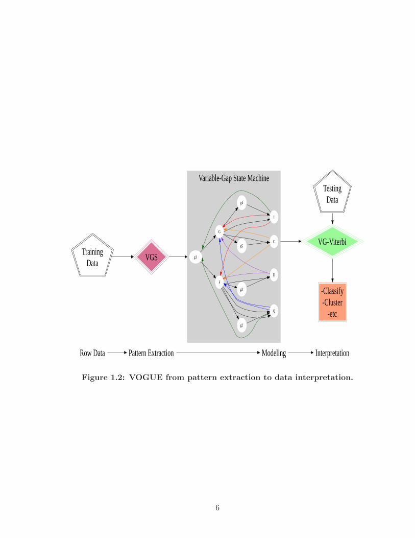
The training and testing of VOGUE consists of three main steps:
1. Pattern Mining via the novel Variable-Gap Sequence (VGS) mining algo-
rithm.
2. Data Modeling via our novel Variable-Order state machine.
3. Interpretation of new data via a modified Viterbi method [27], called Variable-
Gap Viterbi (VG-Viterbi), to model the most probable path through a VOGUE
model.
Figure 1.2 provides a flow chart of VOGUE’s steps from pattern extraction
to data interpretation. A more detailed description of these steps are given in the
following chapters.
4
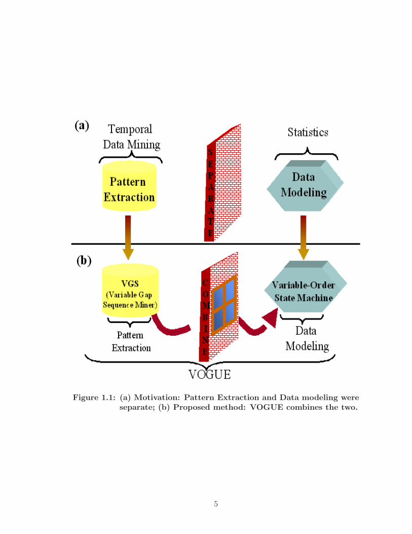
Figure 1.1: (a) Motivation: Pattern Extraction and Data modeling wereseparate; (b) Proposed method: VOGUE combines the two.
5
Variable-Gap State Machine
Row Data Pattern Extraction Modeling Interpretation
VG-Viterbi
-Classify-Cluster
-etc
TestingData
TrainingData
VGS g1
F
G
Q
D
g2
g3
I
C
g4
g5
Figure 1.2: VOGUE from pattern extraction to data interpretation.
6
1.3 Contributions
There are several major contributions of our work:
1. The first major contribution is the combination of two separate but comple-
mentary techniques for modeling and interpreting long range dependencies in
sequential data: data mining and data modeling. The use of data mining for
creating a state machine results in a model that captures the data reference
locality better than a traditional HMM created from the original (noisy) data.
In addition, our approach automatically finds all the dependencies for a given
state, and these need not be of a fixed order, since the mined patterns can be
arbitrarily long. Moreover, the elements of these patterns do not need to be
consecutive, i.e., a variable length gap could exist between the elements. This
enables us to model multiple higher order HMMs via a single variable-order
state machine that executes faster and yields much greater accuracy. This
contribution is composed of:
• a Variable Gap Sequence (VGS) miner, which is a contribution in the area
of pattern extraction. VGS mines frequent patterns with different lengths
and gaps between the elements across and within several sequences. VGS
can be used individually as well as part of VOGUE for pattern extraction.
• a VOGUE state machine that uses the mined variable-gap sequences from
VGS to model multiple higher order HMMs via a single variable-order
state machine.
Moreover, we applied VOGUE to a real world problem, namely, finding ho-
7
mologous proteins. Although VOGUE has a much wider applicability, such
as in web accesses, text mining, user behavior analysis, etc, in this work we
apply VOGUE to a real world problem in biological sequence analysis, namely,
multi-class protein classification. Given a database of protein sequences, the
goal is to build a statistical model so that we can determine whether a query
protein belongs to a given family (class) or not. Statistical models for pro-
teins, such as profiles, position-specific scoring matrices, and hidden Markov
models [30] have been developed to find homologs. However, in most biolog-
ical sequences, interesting patterns repeat (either within the same sequence
or across sequences) and may be separated by variable length gaps. There-
fore a method like VOGUE that specifically takes these kind of patterns into
consideration can be very effective. We show experimentally that VOGUE’s
modeling power is superior to higher-order HMMs while reducing the latter’s
state-space complexity, and improving their prediction. VOGUE also outper-
forms HMMER [30], a HMM model especially designed for protein sequences.
2. The second contribution is in the area of data interpretation and decoding.
This contribution is a consequence of the unique structure of VOGUE sate
machine, where the gaps have a notion of duration. Therefore, we adjusted
the widely used Viterbi algorithm, that solves the interpretation problem, to
meet those needs. We call this method Variable-Gap Viterbi (VG-Viterbi). We
optimized VG-Viterbi based on the fact that the transition matrix between
the states of the model is a sparse matrix and so there is no need to model
8
the transitions between all the states.
3. The third contribution is Canonical VOGUE (C-VOGUE) that aims at in-
creasing the already “good” performance of VOGUE by eliminating artifacts
in the extracted patterns, hence reducing the number of patterns to be mod-
eled later on. These artifacts are retained as being frequent patterns but each
one of these patterns is in fact an artifact of another pattern. This contribu-
tion aims at decreasing the state space complexity of the state machine, which
is a major step towards one of the three goals of modeling with state machines
while keeping good accuracy and coverage.
4. VOGUE is adaptable enough to allow for inclusion of domain specific knowl-
edge to better model patterns with higher order structures unlike other tech-
niques that are made specially for 1 dimensional patterns, and perform poorly.
We achieved this by S-VOGUE (Substitution VOGUE), where the mined pat-
terns are chosen not only based on the frequency of exact match items but
also among items that could be substituted by one another according to their
secondary or tertiary structure. This is, in fact, very helpful in protein anal-
ysis where proteins of the same family share common patterns (motifs) that
are not based on exact match but rather on substitutions based on the protein
sequences elements weight, charge, and hydrophobicity. These elements are
called amino acids.
9
1.4 Thesis Outline
The rest of the chapters are organized as follows: Chapter 2, provides a lit-
erature review of sequential data mining techniques. Then VGS, our new sequence
mining algorithm used to build the VOGUE state machine, is presented. In Chapter
3, we provide a literature review and definition of HMMs, and we present the Baum-
Welch algorithm. In the same chapter we describe our variable-order state machine,
its parameters and structure estimation via VGS. Moreover, we describe the gen-
eralization of VOGUE to mine and model sequences of any length k ≥ 2. Then,
in Chapter 4, we extend VOGUE to Domain Knowledge VOGUE (K-VOGUE) to
allow for substitutions, and Canonical VOGUE (C-VOGUE) to eliminate artifacts
that exist in the patterns mined by VGS. In Chapter 5, we present a literature
review of the Viterbi algorithm [75] that solves the decoding and interpretation
problem in HMMs. Then VG-Viterbi, our adaptation of the Viterbi algorithm, and
its optimization are presented in the same chapter. In Chapter 6, we present exper-
iments and analysis of VOGUE compared to some state of the art techniques in the
application domain of multi-family protein classification. Chapter 7 concludes this
thesis with a summary and provides some future directions.
10

Chapter 2Pattern Mining Using
Sequence Mining
Searching for patterns is one of the main goals in data mining. Patterns have impor-
tant applications in many Knowledge-Discovery and Data mining (KDD) domains
like rule extraction or classification. Data mining can be defined as “the nontrivial
extraction of implicit, previously unknown, and potentially useful information from
data” [40] and “the science of extracting useful information from large data sets
or databases” [45]. Data mining involves the process of analyzing data to show
patterns or relationships; sorting through large amounts of data; and picking out
pieces of relative information or patterns that occur e.g., picking out statistical in-
formation from some data [31]. There are several data mining techniques, such
as association rules, sequence mining [83], classification and regression, similarity
search and deviation detection [35, 44, 46, 90, 91, 92]. Most of the real world appli-
cations encompass sequential and temporal data. For example, analysis of biological
sequences sush as DNA, proteins, etc. Another example is in web prefetching, where
pages are accessed in a session by a user in a sequential manner. In this type of data
each “example” is represented as a sequence of “events”, where each event might be
11
described by a set of attributes. Sequence Mining helps to discover frequent sequen-
tial attributes or patterns across time or positions in a given data set. In the domain
of web usage, a database would be the web page accesses. Here the attribute is a
web page and the object is the web user. The sequences of most frequently accessed
pages are the discovered “frequent” patterns. Biological sequence analysis [37, 101],
identifying plan failures [99], and finding network alarms [47], constitute some of
the real world applications where sequence mining is applied.
In this work, we will explore sequence mining as a mining technique. We
prefer to use sequence mining rather than association mining due to the fact that
association mining discovers only intra-itemsets patterns where items are unordered,
while sequence mining discovers inter-itemsets, called sequences, where items are
ordered [98].
This chapter is organized as follows: in Section 2.1, we provide a definition
of sequence mining, and Section 2.2 provides an overview of related work; and in
Section 2 we present the description of a sequence mining algorithm, cSPADE [97],
that will be used as a base for our proposed algorithm Variable-Gap Sequence miner
(VGS) described in Section 2.5.
2.1 Sequence Mining discovery: Definitions
The problem of mining sequential patterns, as defined in [4] and [83], is
as follows: Let’s consider I = {I1, · · · Im} be the set of m distinct items. An
itemset is a subset of I with possibly un-ordered items. A sequence S, on the
other hand, is an ordered list of itemsets from I (i.e., S = I1, · · · Il where Ij ⊆ I and
12
1 ≤ j ≤ l). S can be defined as S = I1 → I2 · · · → Il, where “→” is a “happen after”
relationship denoted as Ii ¹ Ij and i ≤ j. The length of the sequence S is defined as
| S |=∑
j | Ij |, where | Ij | is the number of items in the itemset Ij. For example,
let’s consider the sequence S = AB → C → DF . This sequence is composed of 3
itemsets, namely, AB, C, and DF , and its length is | S |=| AB | + | C | + | DF |
= 5. The sequence S is then called 5-sequence. We will refer for the remaining of
this proposal to a sequence of length k as k-sequence.
A sequence S ′ = I ′1, · · · I
′p is called a subsequence of S, with p ≤| S |, if there
exist a list of itemsets of S, Ii1 , · · · Iip such that Ij ⊆ I ′ik
, 1 ≤ k, j ≤ p. For example,
the sequence S ′ = A → D is a subsequence of S (described in the previous example),
because A ⊆ AB, D ⊆ DF , and the order of itemsets is preserved. Let D, a set
of sequences, be a sequential database, where each sequence S ∈ D has a unique
identifier, denoted as sid, and each itemset in S has a unique identifier, denoted as
eid. The support of S’, is defined as the fraction of the database sequences that
contain S’, given as σD(s′) =| Ds | / | D |, where Ds′ is a set, contained in D,
of database sequences S such that S ′ ⊆ S. A sequence is said to be frequent if it
occurs more than a user-specified threshold minsup, called minimum support. The
problem of mining frequent patterns is to find all frequent sequences in the database.
This is formally defined in [83] as:
Definition (Sequential Pattern Mining): Given a sequential database D
and a user-specified minsupparameter σ (0 ≤ σ ≤ 1), find all sequences each of
which is supported by at least ⌈σ | D |⌉ of sequences in D.
13
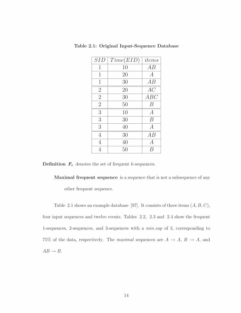
Table 2.1: Original Input-Sequence Database
SID Time(EID) items
1 10 AB
1 20 A
1 30 AB
2 20 AC
2 30 ABC
2 50 B
3 10 A
3 30 B
3 40 A
4 30 AB
4 40 A
4 50 B
Definition Fk denotes the set of frequent k-sequences.
Maximal frequent sequence is a sequence that is not a subsequence of any
other frequent sequence.
Table 2.1 shows an example database [97]. It consists of three items (A,B,C),
four input sequences and twelve events. Tables 2.2, 2.3 and 2.4 show the frequent
1-sequences, 2-sequences, and 3-sequences with a min sup of 3, corresponding to
75% of the data, respectively. The maximal sequences are A → A, B → A, and
AB → B.
14
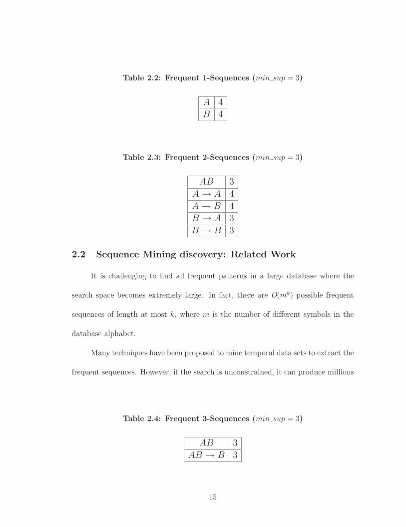
Table 2.2: Frequent 1-Sequences (min sup = 3)
A 4
B 4
Table 2.3: Frequent 2-Sequences (min sup = 3)
AB 3
A → A 4
A → B 4
B → A 3
B → B 3
2.2 Sequence Mining discovery: Related Work
It is challenging to find all frequent patterns in a large database where the
search space becomes extremely large. In fact, there are O(mk) possible frequent
sequences of length at most k, where m is the number of different symbols in the
database alphabet.
Many techniques have been proposed to mine temporal data sets to extract the
frequent sequences. However, if the search is unconstrained, it can produce millions
Table 2.4: Frequent 3-Sequences (min sup = 3)
AB 3
AB → B 3
15
of rules. Moreover, some constrains might need to be added in some domains. For
example, a user might be interested in searching for sequences occurring close in
time to each other or far apart from each other, those that contain some specific
items, occurring during a specific period of time, or frequent at most a number of
times or at least another number of times in the data set.
Several techniques have been proposed to discover the frequent sequences
[5, 70, 63, 99]. One of the early algorithms that efficiently discovered the frequent
sequences is the AprioriAll [83], that iteratively finds itemsets of length l based on
previously generated (l-1)-length frequent itemsets. In [49] frequent sequences in a
single long input-sequence, called frequent episodes, were mined. It was extended to
discover generalized episodes that allow uniary conditions on individual sequences
itemsets, or binary conditions on itemset pairs [62]. In [3], the Generalized Sequen-
tial Patterns (GSP) algorithm was proposed to extend the AprioriAll algorithm
by introducing user-specified minimum gap and maximum gap time constraints,
user-specified sliding window size, and user-specified minimum support. GSP is
an iterative algorithm that counts candidate frequent sequences of length k in the
k−th database scan. However, GSP suffers from a number of drawbacks, namely, it
needs as many full scans of the database as the longest frequent sequence; it uses a
complex hash structure with poor locality; and it scales up linearly as the size of the
data increases. SPADE [98] was proposed to cope with GSP ’s drawbacks. SPADE
uses a vertical id-list database, prefix-based equivalence classes, and it enumerates
frequent sequences through simple temporal joins. SPADE uses dynamic program-
ming concepts to break the large search space of frequent patterns into small and
16
independent chunks. It requires only three scans over the database as opposed to
GSP which requires multiple scans, and SPADE has the capacity of in-memory
computation and parallelization which can considerably decrease the computation
time. SPADE was later on extended to Constraint SPADE (cSPADE ) [97] which
considers constraints like max/min gaps and sliding windows. SPIRIT [42] is a fam-
ily of four algorithms for mining sequences that are a complementary to cSPADE.
However, cSPADE considers a different constraint that finds sequences predictive
of at least one class for temporal classification problems. In fact, SPIRIT mines
sequences that match user-specified regular-expression constraints. The most re-
laxed of the four is SPIRIT(N) that eliminates items not appearing in any of the
user specified regular-expressions. The most strict one is SPIRIT(R), that applies
the constraints, while mining and only outputs the exact set. GenPresixSpan [6] is
another algorithm based on PrefixSpan [72] that considers gap-constraints. Regu-
lar expressions and other constraints have been studied in [53, 43, 101]. In [53], a
mine-and-examine paradigm for interactive exploration of association and sequence
episodes was presented, where a large collection of frequent patterns is first to be
mined and produced. Then the user can explore this collection by using “templates”
that specify what is of interest and what is not. In [68], CAP algorithm was pro-
posed to extract all frequent associations matching a large number of constraints.
However, because of the constrained associations, these methods are unsuitable for
temporal sequences that introduce different kinds of constraints.
Since cSPADE is an efficient and scalable method for mining frequent se-
quences, we will use it as a base for our new method Variable-Gap Sequence miner
17
(VGS), to extract the patterns that will be used to estimate the parameters and
structure of our proposed VOGUE state machine. The main difference, however,
between VGS and cSPADE is that cSPADE essentially ignores the length and sym-
bol distributions of gaps, whereas VGS is specially designed to extract such patterns
within one or more sequences. Note that while other methods can also mine gapped
sequences [6, 43, 101], the key difference is that during mining VGS explicitly keeps
track of all the intermediate symbols, their frequency, and the gap frequency distri-
bution, which are used to build VOGUE.
Before we go into more details about cSAPDE, we will give an overview of
SPADE algorithm in Section 1, since cSPADE is an extension of it. cSPADE tech-
nique will be described in the Section 2. Section 2.5 provides the details of our
proposed method VGS.
2.3 SPADE: Sequential Patterns Discovery using Equivalence
classes
The SPADE algorithm [98] is developed for fast mining of frequent sequences.
Given as input a sequential database D and the minimum support, denoted as
min sup, the main steps of SPADE consists of the following:
1. Computation of the frequent 1-sequences:
F1 = { frequent items or 1-sequences};
2. Computation of the frequent 2-sequences:
18
F2 = { frequent items or 2-sequences };
3. Decomposition into prefix-based parent equivalence classes:
ξ = { equivalence classes [X]θ1};
4. Enumeration of all other sequences, using Breadth-First Search (BFS ) or
Depth-First Search (DFS ) techniques, within each class [X] in ξ.
In the above, i-sequences denotes sequences of length i, 1 ≤ i ≤ 2.
19
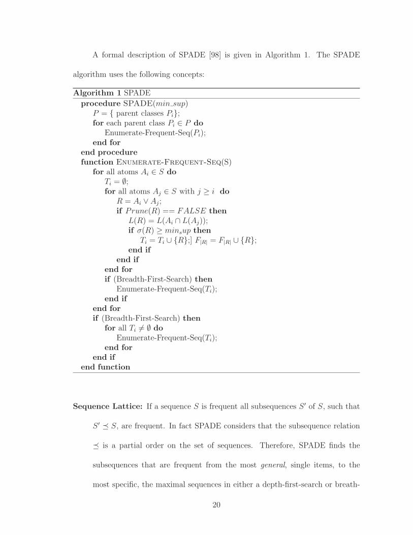
A formal description of SPADE [98] is given in Algorithm 1. The SPADE
algorithm uses the following concepts:
Algorithm 1 SPADE
procedure SPADE(min sup)P = { parent classes Pi};for each parent class Pi ∈ P do
Enumerate-Frequent-Seq(Pi);end for
end procedurefunction Enumerate-Frequent-Seq(S)
for all atoms Ai ∈ S doTi = ∅;for all atoms Aj ∈ S with j ≥ i do
R = Ai ∨ Aj;if Prune(R) == FALSE then
L(R) = L(Ai ∩ L(Aj));if σ(R) ≥ minsup then
Ti = Ti ∪ {R};] F|R| = F|R| ∪ {R};end if
end ifend forif (Breadth-First-Search) then
Enumerate-Frequent-Seq(Ti);end if
end forif (Breadth-First-Search) then
for all Ti 6= ∅ doEnumerate-Frequent-Seq(Ti);
end forend if
end function
Sequence Lattice: If a sequence S is frequent all subsequences S ′ of S, such that
S ′ ¹ S, are frequent. In fact SPADE considers that the subsequence relation
¹ is a partial order on the set of sequences. Therefore, SPADE finds the
subsequences that are frequent from the most general, single items, to the
most specific, the maximal sequences in either a depth-first-search or breath-
20
first-search manner. This is done by looking into the sequence lattice spanned
by the subsequence (¹) relation as shown in Figure 2.1 for the example dataset.
Frequent Sequence Lattice
3AB->B
3AB
4A->B
3B->B
SID
1
2
4
EID
10
30
30
Intersect A->B and B->B
4A->A
4A
3B->A
4B
SID
1
2
2
3
4
4
EID
10
20
30
10
30
40
Intersect A and B
SID
1
1
2
4
EID
10
20
30
30
{}
Figure 2.1: Frequent Sequence Lattice and Temporal Joins.
Support Counting: One of the main differences between SPADE and the other
sequence mining algorithms [5, 83] is that the latter ones consider a horizontal
database layout whereas SPADE considers a vertical one. The database in the
horizontal format consists of a set of input sequences which in their turn consist
of a set of events and the items contained in the events. The vertical database,
on the other hand, consists of an a disk-based id-list, denoted L(X) for each
21
item X in the sequence lattice, where each entry of the id-list is a pair of
sequence id and event id (sid, eid) where the item occurs. For example, let’s
consider the database described in Table 2.1, the id-list consist of the tuples
{(2, 20), (2, 30)}.
With the vertical layout in mind, the computation of F1 and F2 becomes as
follows:
Computation of F1 : The id-list of each database item is read from disk
into memory. Then the id-list is scanned incrementing the new sid en-
countered. All this is done in a single database scan.
Computation of F2 : Let N = |F1| be the number of frequent items, and
A the average id-list size in bytes. In order to compute F2 a naive im-
plementation will require(
N2
)
id-list joins for all pairs of items. Then,
(A×N×(N−1)2 ) is the corresponding amount of data read; this is
almost N/2 data scans. To avoid this inefficient method two alternate
solutions were proposed in [97]:
1. To compute F2 above a user specified lower bound threshold, a pre-
processing step is used.
2. An on-the-fly vertical-to-horizontal transformation is performed: scan
the id-list of each item i into memory. Then for each (sid, eid) pair
(i, e) is inserted in the list for input sequence S. Using the id-list for
item A from the previous example in Table 2.1, the first pair (1, 15)
is scanned then (A, 15) is inserted in the list for input-sequence 1.
22

Table 2.5 describes the complete vertical-to-horizontal transforma-
tion of the database. To recover the horizontal database, for each
sid, a list of all 2 − sequences is formed in the list, and counts are
updated in a 2 − dimensional array indexed by the frequent items.
Then, as shown in Figure 2.1, the intermediate id-list for A → B is
obtained by a temporal join on the lists of A and B. All occurrences of
A “before” B, that represent A → B are found in an input sequence
and the corresponding eids are stored to obtain L(A → B). In the
case of AB → B, the id-lists of its two generating sequences A → B
and B → B are joined. Because of main-memory limitations, it is not
possible to enumerate all the frequent sequences by traversing the lattice
and performing joins. However, this large search space is decomposed by
SPADE into smaller chunks, called classes, to be processed separately by
using suffix-based equivalence classes.
Definition : Two k-sequences are in the same class if they share a com-
mon k − 1 length suffix.
Therefore, each class is a sub-lattice of the original lattice. It can be
processed independently since it contains all the information to generate
all frequent sequences with the same suffix. SPADE recursively calls the
procedure Enumerate-Frequent that counts the suffix classes starting from
suffix-classes of length one (called parent classes), in the running example
(A, B), then it uses suffix-classes of length two, in the running example
23
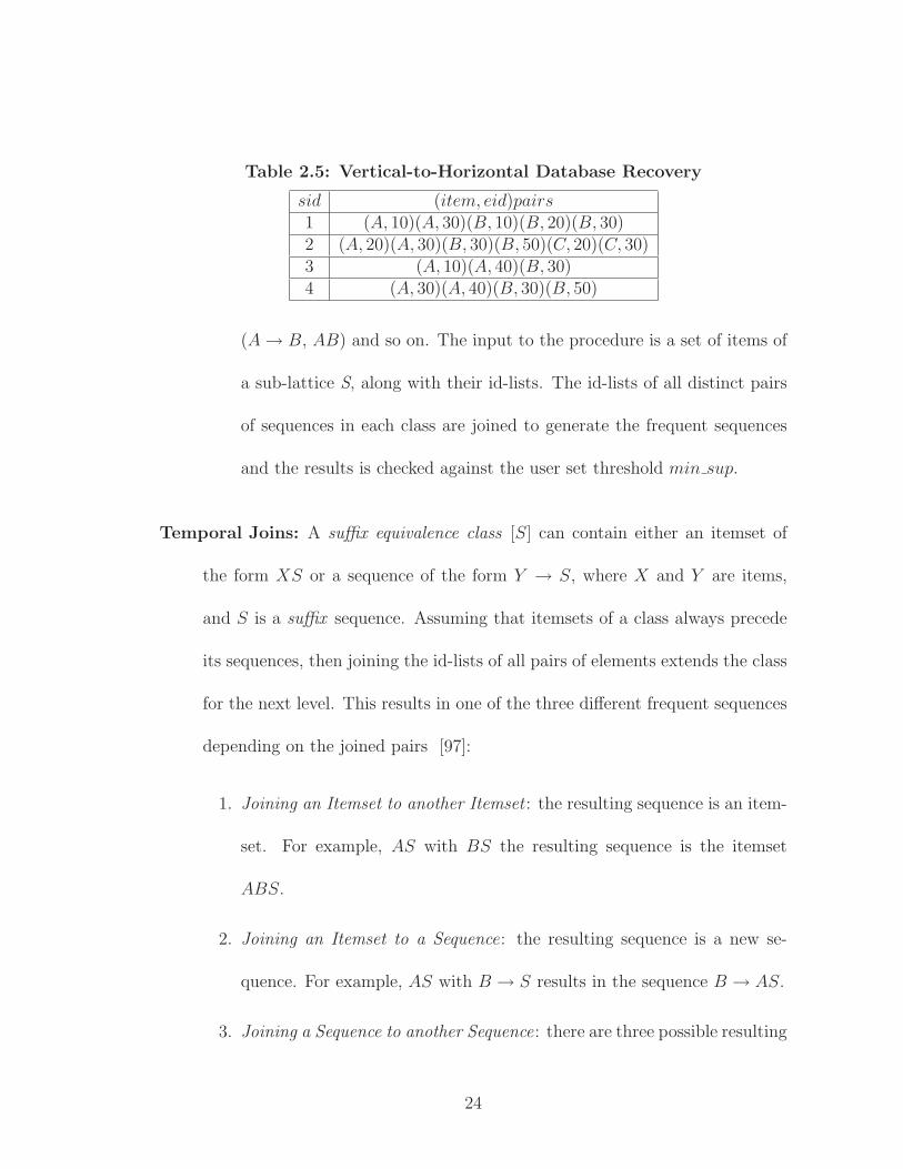
Table 2.5: Vertical-to-Horizontal Database Recovery
sid (item, eid)pairs1 (A, 10)(A, 30)(B, 10)(B, 20)(B, 30)2 (A, 20)(A, 30)(B, 30)(B, 50)(C, 20)(C, 30)3 (A, 10)(A, 40)(B, 30)4 (A, 30)(A, 40)(B, 30)(B, 50)
(A → B, AB) and so on. The input to the procedure is a set of items of
a sub-lattice S, along with their id-lists. The id-lists of all distinct pairs
of sequences in each class are joined to generate the frequent sequences
and the results is checked against the user set threshold min sup.
Temporal Joins: A suffix equivalence class [S] can contain either an itemset of
the form XS or a sequence of the form Y → S, where X and Y are items,
and S is a suffix sequence. Assuming that itemsets of a class always precede
its sequences, then joining the id-lists of all pairs of elements extends the class
for the next level. This results in one of the three different frequent sequences
depending on the joined pairs [97]:
1. Joining an Itemset to another Itemset : the resulting sequence is an item-
set. For example, AS with BS the resulting sequence is the itemset
ABS.
2. Joining an Itemset to a Sequence: the resulting sequence is a new se-
quence. For example, AS with B → S results in the sequence B → AS.
3. Joining a Sequence to another Sequence: there are three possible resulting
24
sequences considering the sequences A → S and B → S: a new itemset
AB → S, the sequence A → B → S or the sequence B → A → S.
From Figure 2.1, from the 1−sequences A and B we can get three sequences:
the itemset AB and the two sequences A → B and its “reverse” B → A.
To obtain the id-list of itemset AB, the equality of (sid,eid) pairs needs to
be checked and in this case it is L(AB) = {(1, 10), (1, 30), (2, 20), (4, 30)} in
Figure 2.1. This shows that AB is frequent in 3 out of the 4 sequences in the
data set (min sup = 3 which corresponds to 75% of the data). In the case of
the resulting sequence A → B, there is need to check for (sid,eid) pairs where
sid for both A and B are the same but the eid for B is strictly greater in
time than the one for A. The (sid,eid) pairs in the resulting id-list for A → B
only keep the information about the first item A and not B. This is because
all members of a class share the same suffix and hence the same eid for that
suffix.
2.4 cSPADE: constrained Sequential Patterns Discovery us-
ing Equivalence classes
In this section we describe in some detail the cSPADE algorithm [97]. cSPADE
is designed to discover the following types of patterns:
1. Single item sequences as well as the sequences of subsets of items. For example
the set AB, and AB → C in (AB → C → DF ).
2. Sequences with variable gaps among itemsets ( a gap of 0 will discover the
25
sequences with consecutive itemsets). For example, from the sequence (AB →
C → DF ), AB → DF is a subsequence of gap 1 and AB → C is a subsequence
of gap 0.
cSPADE is an extension of the Sequential Patterns Discovery using Equivalence
classes (SPADE) algorithm by adding the following constraints:
1. Length and width restrictions.
2. Minimum gap between sequence elements.
3. Maximum gap between sequence elements.
4. A time window of occurrence of the whole sequence.
5. Item constraints for including or excluding certain items.
6. Finding sequences distinctive of at least a special attribute-value pair.
Definition : A Constraint [97] is said to be class-preserving if in the presence
of the constraint suffix-class retains it’s self-containment property, i.e., sup-
port of any k-sequence can be found by joining id-lists of its two generating
subsequences of length (k − 1) within the same class.
If a constraint is class-preserving [97], the frequent sequences satisfying that
constraint can be listed using local suffix class information only. Among all the
constraints stated above, the maximum gap constraint is the only one that is not
class-preserving. Therefore, there is a need for a different enumeration method.
cSPADE pseudo-code is described in Algorithm 2.
26
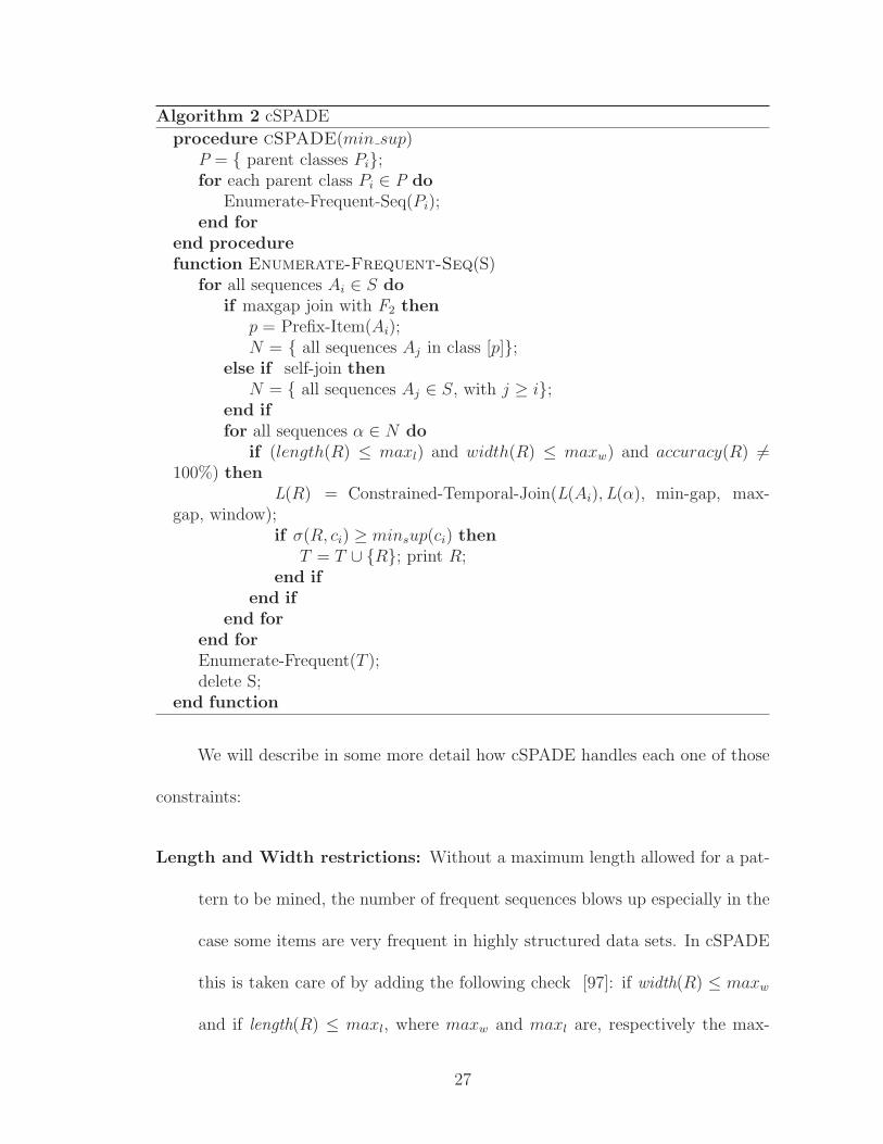
Algorithm 2 cSPADE
procedure cSPADE(min sup)P = { parent classes Pi};for each parent class Pi ∈ P do
Enumerate-Frequent-Seq(Pi);end for
end procedurefunction Enumerate-Frequent-Seq(S)
for all sequences Ai ∈ S doif maxgap join with F2 then
p = Prefix-Item(Ai);N = { all sequences Aj in class [p]};
else if self-join thenN = { all sequences Aj ∈ S, with j ≥ i};
end iffor all sequences α ∈ N do
if (length(R) ≤ maxl) and width(R) ≤ maxw) and accuracy(R) 6=100%) then
L(R) = Constrained-Temporal-Join(L(Ai),L(α), min-gap, max-gap, window);
if σ(R, ci) ≥ minsup(ci) thenT = T ∪ {R}; print R;
end ifend if
end forend forEnumerate-Frequent(T );delete S;
end function
We will describe in some more detail how cSPADE handles each one of those
constraints:
Length and Width restrictions: Without a maximum length allowed for a pat-
tern to be mined, the number of frequent sequences blows up especially in the
case some items are very frequent in highly structured data sets. In cSPADE
this is taken care of by adding the following check [97]: if width(R) ≤ maxw
and if length(R) ≤ maxl, where maxw and maxl are, respectively the max-
27
imum width and length allowed in a sequence. This addition is done in the
“Enumerate” method as shown in cSPADE’s pseudo-code. These constraints
are class-preserving since they do not affect id-lists.
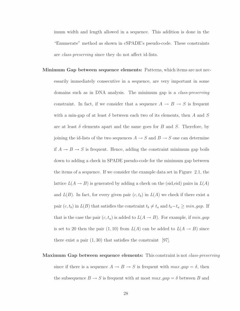
Minimum Gap between sequence elements: Patterns, which items are not nec-
essarily immediately consecutive in a sequence, are very important in some
domains such as in DNA analysis. The minimum gap is a class-preserving
constraint. In fact, if we consider that a sequence A → B → S is frequent
with a min-gap of at least δ between each two of its elements, then A and S
are at least δ elements apart and the same goes for B and S. Therefore, by
joining the id-lists of the two sequences A → S and B → S one can determine
if A → B → S is frequent. Hence, adding the constraint minimum gap boils
down to adding a check in SPADE pseudo-code for the minimum gap between
the items of a sequence. If we consider the example data set in Figure 2.1, the
lattice L(A → B) is generated by adding a check on the (sid,eid) pairs in L(A)
and L(B). In fact, for every given pair (c, tb) in L(A) we check if there exist a
pair (c, tb) in L(B) that satisfies the constraint tb 6= ta and tb−ta ≥ min gap. If
that is the case the pair (c, ta) is added to L(A → B). For example, if min gap
is set to 20 then the pair (1, 10) from L(A) can be added to L(A → B) since
there exist a pair (1, 30) that satisfies the constraint [97].
Maximum Gap between sequence elements: This constraint is not class-preserving
since if there is a sequence A → B → S is frequent with max gap = δ, then
the subsequence B → S is frequent with at most max gap = δ between B and
28
S but A → S is only frequent at most max gap = 2δ. Therefore, if A → S
could be infrequent with this constraint but yet A → B → S is frequent. To
incorporate maximum gap constraint to the SPADE pseudo-code [97], first a
check needs to be added such that, in the example of Figure 2.1, for a given
pair (c, ta) in L(A), check if a pairs (c, tb) exists in L(B) such that tb 6= ta
and tb − ta ≤ max gap. The second step is to change the enumeration of
the sequences with the maximum gap constraint. A join with F2 is necessary
instead of a self-join because the classes are no more self-contained. This join
is done recursively with F2 until no extension is found to be frequent.
Time Window of occurrence of the whole sequence: In other words, the time
constraint applies to the whole sequence instead of minimum or maximum
gap between elements of the sequence [97]. This constraint is class-preserving
since if a sequence A → B → S is within a time-window δ, then it implies
that A → S and B → S are within the same window and so on for any sub-
sequence. However, including the time-window into the SPADE software is
difficult because the information concerning the whole sequence time is lost
from the parent class. In fact, only the information about the eid of the first
item of the sequence is stored and the one of the remaining items is lost from
one class to the next. The solution proposed in [97] is to keep information
about the difference “diff” between the eid of the first and the last item of the
sequence at each step of the process. This is done by adding an extra column
in the id-list called diff to store that information.
29
Item constraints for including or excluding certain items: The use of a ver-
tical format of the data set and the equivalence classes in cSPADE makes it
easy to add constraints on items within sequences [97]. For instance, if the
constraint is excluding a certain item from the frequent sequences, then remov-
ing it from parent classes takes care of that. Therefore, no frequent sequence
will contain that item. The same procedure will apply in the case of including
an item.
Whereas cSPADE essentially ignores the length and symbol distributions of
gaps, the new mining sequence algorithm that we present in the work, VGS (Variable-
Gap Sequences), is specially designed to extract such patterns within one or more
sequences. The next Chapter describes VGS in more details.
2.5 Pattern Extraction: Variable-Gap Sequence (VGS) miner
Variable-Gap Sequence miner (VGS) is based on cSPADE [97]. While cSPADE
essentially ignores the length and symbol distributions of gaps, VGS is specially
designed to extract such patterns within one or more sequences. Note that whereas
other methods can also mine gapped sequences [6, 83, 97, 101], the key difference is
that during mining VGS explicitly keeps track of all the intermediate symbols, their
frequency, and the gap frequency distributions, which are used to build VOGUE.
VGS takes as input the maximum gap allowed (maxgap), the maximum se-
quence length (k), and the minimum frequency threshold (min sup). VGS mines
all sequences having up to k elements, with no more than maxgap gaps between
30
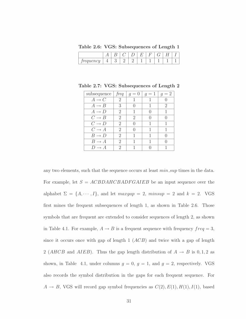
Table 2.6: VGS: Subsequences of Length 1
A B C D E F G H Ifrequency 4 3 2 2 1 1 1 1 1
Table 2.7: VGS: Subsequences of Length 2
subsequence freq g = 0 g = 1 g = 2A → C 2 1 1 0A → B 3 0 1 2A → D 2 1 0 1C → B 2 2 0 0C → D 2 0 1 1C → A 2 0 1 1B → D 2 1 1 0B → A 2 1 1 0D → A 2 1 0 1
any two elements, such that the sequence occurs at least min sup times in the data.
For example, let S = ACBDAHCBADFGAIEB be an input sequence over the
alphabet Σ = {A, · · · , I}, and let maxgap = 2, minsup = 2 and k = 2. VGS
first mines the frequent subsequences of length 1, as shown in Table 2.6. Those
symbols that are frequent are extended to consider sequences of length 2, as shown
in Table 4.1. For example, A → B is a frequent sequence with frequency freq = 3,
since it occurs once with gap of length 1 (ACB) and twice with a gap of length
2 (AHCB and AIEB). Thus the gap length distribution of A → B is 0, 1, 2 as
shown, in Table 4.1, under columns g = 0, g = 1, and g = 2, respectively. VGS
also records the symbol distribution in the gaps for each frequent sequence. For
A → B, VGS will record gap symbol frequencies as C(2), E(1), H(1), I(1), based
31

on the three occurrences. Since k = 2, VGS would stop after mining sequences of
length 2. Otherwise, VGS would continue mining sequences of length k ≥ 3, until
all sequences with k elements are mined.
Before we start describing VGS, we will provide definitions of some terms that
will be used in this section and in the rest of this thesis:
k-seq : sequence of length k, i.e. k elements. For example, A → B is 2-seq where
B occurs after A and A → B → C is a 3-seq and so on.
min sup : minimum support, is the minimum threshold for the frequency count of
sequences.
maxgap : maximum gap allowed between any two elements of a k-seq.
F1 : the set of frequent 1-seq (single items).
Fk : the set of all k-seq which frequency is higher than the minimum threshold
min sup and the gap between their elements is at most of length maxgap.
Ck : the set of candidate k-seq.
The first step of VOGUE uses VGS to mine the raw data-set for variable gap
frequent sequences. It takes as input the maximum gap allowed maxgap between
the elements of the subsequences, the maximum length (k) of the subsequences,
and the minimum frequency threshold (min sup) for sequences to be considered
frequent. The mined subsequences from VGS are of the form A → B if k = 2,
or A → B → C if k = 3, and so on. The frequency of the subsequences is cal-
culated either across the sequences in the data-set and/or within the sequences
32
in the data-set, as the application may require. Only those sequences that are
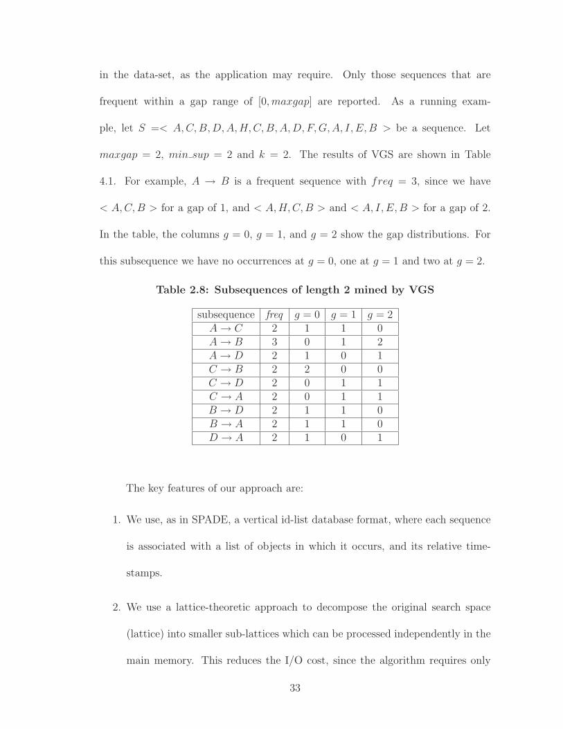
frequent within a gap range of [0,maxgap] are reported. As a running exam-
ple, let S =< A,C,B,D,A,H,C,B,A,D, F,G,A, I, E,B > be a sequence. Let
maxgap = 2, min sup = 2 and k = 2. The results of VGS are shown in Table
4.1. For example, A → B is a frequent sequence with freq = 3, since we have
< A,C,B > for a gap of 1, and < A,H,C,B > and < A, I, E,B > for a gap of 2.
In the table, the columns g = 0, g = 1, and g = 2 show the gap distributions. For
this subsequence we have no occurrences at g = 0, one at g = 1 and two at g = 2.
Table 2.8: Subsequences of length 2 mined by VGS
subsequence freq g = 0 g = 1 g = 2A → C 2 1 1 0A → B 3 0 1 2A → D 2 1 0 1C → B 2 2 0 0C → D 2 0 1 1C → A 2 0 1 1B → D 2 1 1 0B → A 2 1 1 0D → A 2 1 0 1
The key features of our approach are:
1. We use, as in SPADE, a vertical id-list database format, where each sequence
is associated with a list of objects in which it occurs, and its relative time-
stamps.
2. We use a lattice-theoretic approach to decompose the original search space
(lattice) into smaller sub-lattices which can be processed independently in the
main memory. This reduces the I/O cost, since the algorithm requires only
33
three scans of the data set. Refer to [22] for a detailed introduction to Lattice
theory.
VGS is, therefore, cost efficient by reducing the dataset scans and using an
efficient depth first search, as described in [98]. We use, as in [98], a vertical database
format, where an id-list for each item in the dataset.Each entry in the id-list is
a(sid, eid) pair. Eid is where the item exists in sequence which id is sid. sid is the
sequence id in the data set and eid is the event id where the item exists.
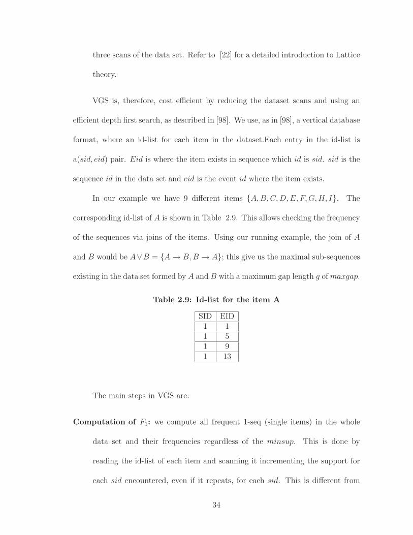
In our example we have 9 different items {A,B,C,D,E, F,G,H, I}. The
corresponding id-list of A is shown in Table 2.9. This allows checking the frequency
of the sequences via joins of the items. Using our running example, the join of A
and B would be A∨B = {A → B,B → A}; this give us the maximal sub-sequences
existing in the data set formed by A and B with a maximum gap length g of maxgap.
Table 2.9: Id-list for the item A
SID EID1 11 51 91 13
The main steps in VGS are:
Computation of F1: we compute all frequent 1-seq (single items) in the whole
data set and their frequencies regardless of the minsup. This is done by
reading the id-list of each item and scanning it incrementing the support for
each sid encountered, even if it repeats, for each sid. This is different from
34
SPADE where only new sid are taken into considerations to look for patterns
across only the sequences. In VGS we look for patterns within and across the
sequences in the data set.
Computation of F2: we compute all the 2-seq with a gap of length g between
its elements, g ∈ {0, · · · ,maxgap} in which frequencies are greater than the
min sup. g = 0 corresponds to no elements between two main elements of the
k-seq, and g = 1 corresponds to one element between two main elements of
the elements of the k-seq and so on. This computation is done by scanning
the id-list of each item in the alphabet into memory. For each pair (sid, eid)
we insert it in the list for the input sequence whose id is sid. We, then, form
a list of all 2-sequences in the list for each sid, and increment the frequency if
the difference between the two eid events is less than the maxgap allowed.
Enumeration of all other frequent k-seq, with frequency at least min-sup, with
variable gaps between each two of its elements via Depth First Search (DFS)
within each class. For example, the 3-sequence Ag1−→ B
g1−→ C has with
gap g1 ∈ {0, · · · ,maxgap} between A and B and gap g2 ∈ {0, · · · ,maxgap}
between B and C. Where “Ag1→ B” means A is followed by B after g1 elements
in between them. Likewise, “Bg2→ C” means B is followed by C after g2
elements in between them. The procedure is described in Algorithm 3.
The input to the procedure is a set of items of a sub-lattice S, along with
their id-lists and the min sup and maxgap. The sequences that are found to
be frequent form the atoms of classes for the next level. This process is done
35
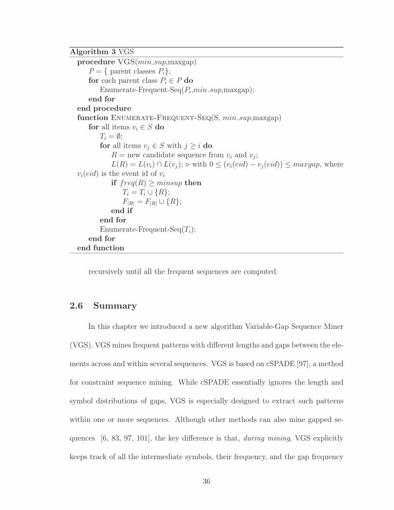
Algorithm 3 VGS
procedure VGS(min sup,maxgap)P = { parent classes Pi};for each parent class Pi ∈ P do
Enumerate-Frequent-Seq(Pi,min sup,maxgap);end for
end procedurefunction Enumerate-Frequent-Seq(S, min sup,maxgap)
for all items vi ∈ S doTi = ∅;for all items vj ∈ S with j ≥ i do
R = new candidate sequence from vi and vj;L(R) = L(vi) ∩ L(vj); ⊲ with 0 ≤ (vi(eid) − vj(eid)) ≤ maxgap, where
vi(eid) is the event id of vi
if freq(R) ≥ minsup thenTi = Ti ∪ {R};F|R| = F|R| ∪ {R};
end ifend forEnumerate-Frequent-Seq(Ti);
end forend function
recursively until all the frequent sequences are computed.
2.6 Summary
In this chapter we introduced a new algorithm Variable-Gap Sequence Miner
(VGS). VGS mines frequent patterns with different lengths and gaps between the ele-
ments across and within several sequences. VGS is based on cSPADE [97], a method
for constraint sequence mining. While cSPADE essentially ignores the length and
symbol distributions of gaps, VGS is especially designed to extract such patterns
within one or more sequences. Although other methods can also mine gapped se-
quences [6, 83, 97, 101], the key difference is that, during mining, VGS explicitly
keeps track of all the intermediate symbols, their frequency, and the gap frequency
36

distribution. VGS can be used individually or as part of the “pattern extraction”
step in VOGUE. The information that VGS extracts from the mined sequences are
used in the “modeling” step of VOGUE. The next chapter describes how in the
“modeling” step of VOGUE the mined patterns from VGS are used to build a new
state machine that we call Variable-Order State machine.
37
Chapter 3Data Modeling Using
Variable-Order State
Machine
In the late sixties and early seventies, Baum and his colleagues published the basic
theory of Hidden Markov Models (HMMs) [11, 14, 15, 12, 13]. HMMs are a rich
mathematical structure that can be applied to a variety of applications. However,
they only became a popular probabilistic framework for modeling processes that
have structure in time, starting in the mid 80’s. That was mainly because the
basic theory of HMMs was published in mathematical journals that was not read
by engineers.
HMMs quantize a system’s configuration space into a number of discrete states
with probabilities to transit between those states. The current state of the system
is indexed in a single finite discrete variable when the system’s structure is in time
domain. This variable’s value encompasses the past information about the process
and is used later on for future inferences.
HMMs are a powerful statistical tool that have been applied in a variety of
problems ranging from speech recognition, to biological sequence analysis, to robot
planning, to web prefetching. Speech recognition, however, is the area of research
38

where a considerable amount of papers and books on using HMM have been pro-
duced [58, 78]. The best description of how HMMs have been used in Speech
recognition is described in the well referenced tutorial by Rabiner [75]. As biologi-
cal knowledge accumulates, HMMs have been used as one of the statistical structures
for biological sequence analysis, a growing field of research, from human genomes to
protein folding problems, [27]. In [29], Profile HMMs have been used for multiple
alignment of conserved sequences. HMMs have been used as well in inferring phy-
logenetic trees [71], and in splice site detection [48]. Partially Observable Markov
Decision Process (POMDP) models have been used in robot planning to allow the
robots to act and learn even if they are uncertain about their current location, [54].
In [74], all Kth Markov model have been used to predict web surfing behavior. A
hidden markov model was defined for each character in a text recognition applica-
tion from grey level images in [1]. In [64], an HMM was used for automatic gait
classification in medical image processing.
3.1 Hidden Markov Model: Definitions
In this section, we will provide a overview on the theory of HMMs based on
Rabiner’s tutorial [75].
The fact that only the sequence of observations is observed, but not the states,
explains why these models are called “hidden” Markov Models. As an example, let’s
consider the coin tossing example in Rabiner’s tutorial [75]. Suppose you are in a
room with a barrier, and another person is performing the tossing experiment, with
the possibility that the coin is biased. You are only given the result of heads and
39
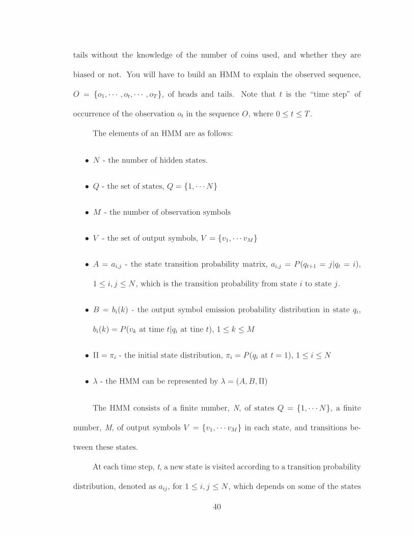
tails without the knowledge of the number of coins used, and whether they are
biased or not. You will have to build an HMM to explain the observed sequence,
O = {o1, · · · , ot, · · · , oT}, of heads and tails. Note that t is the “time step” of
occurrence of the observation ot in the sequence O, where 0 ≤ t ≤ T .
The elements of an HMM are as follows:
• N - the number of hidden states.
• Q - the set of states, Q = {1, · · ·N}
• M - the number of observation symbols
• V - the set of output symbols, V = {v1, · · · vM}
• A = ai,j - the state transition probability matrix, ai,j = P (qt+1 = j|qt = i),
1 ≤ i, j ≤ N , which is the transition probability from state i to state j.
• B = bi(k) - the output symbol emission probability distribution in state qi,
bi(k) = P (vk at time t|qi at tine t), 1 ≤ k ≤ M
• Π = πi - the initial state distribution, πi = P (qi at t = 1), 1 ≤ i ≤ N
• λ - the HMM can be represented by λ = (A,B, Π)
The HMM consists of a finite number, N, of states Q = {1, · · ·N}, a finite
number, M, of output symbols V = {v1, · · · vM} in each state, and transitions be-
tween these states.
At each time step, t, a new state is visited according to a transition probability
distribution, denoted as aij, for 1 ≤ i, j ≤ N , which depends on some of the states
40

visited before. Being in state i, if the transition probability is only dependent on the
previous state (i − 1) (the Markov property), the Markov process is said to satisfy
the first order Markov property:
aij = P (qt+1 = j|qt = i, ..., qt−h = l)
= P (qt+1 = sj|qt = si)
(3.1)
where 1 ≤ i, j, l ≤ N , 1 ≤ h ≤ t − 1, 0 ≤ aij ≤ 1 andN∑
i=1
aij = 1
On the other hand, if the transition probability is dependent on the previous
k -states, the Markov Process is said to satisfy the kth- order Markov property.
After each transition is made, an output symbol is produced according to a
stationary probability density function (PDF) {bi(k), 1 ≤ i ≤ N , 1 ≤ k ≤ M}. It
models the likelihood of observing symbol vk, 1 ≤ k ≤ M , given that the Markov
process is in state i (i.e., the observed symbol depends only on the current state
“i”), denoted:
bi(k) = P (vk at t|qi at t) (3.2)
and again 1 ≤ i ≤ N , 0 ≤ bi(k) ≤ 1 andM∑
k=1
bi(k) = 1.
In addition to the transition probabilities and output symbol probability dis-
tribution, a Markov model also needs a set of initial state probabilities denoted:
πi = P (qi at t = 1), for it to completely determine the probability of observing a
state sequence S = {s1, · · · , st, · · · , sT}:
P (S) = π1
T−1∏
t=1
ast,st+1 (3.3)
41
where π1, the probability of being in state 1 at time t = 1, means that the
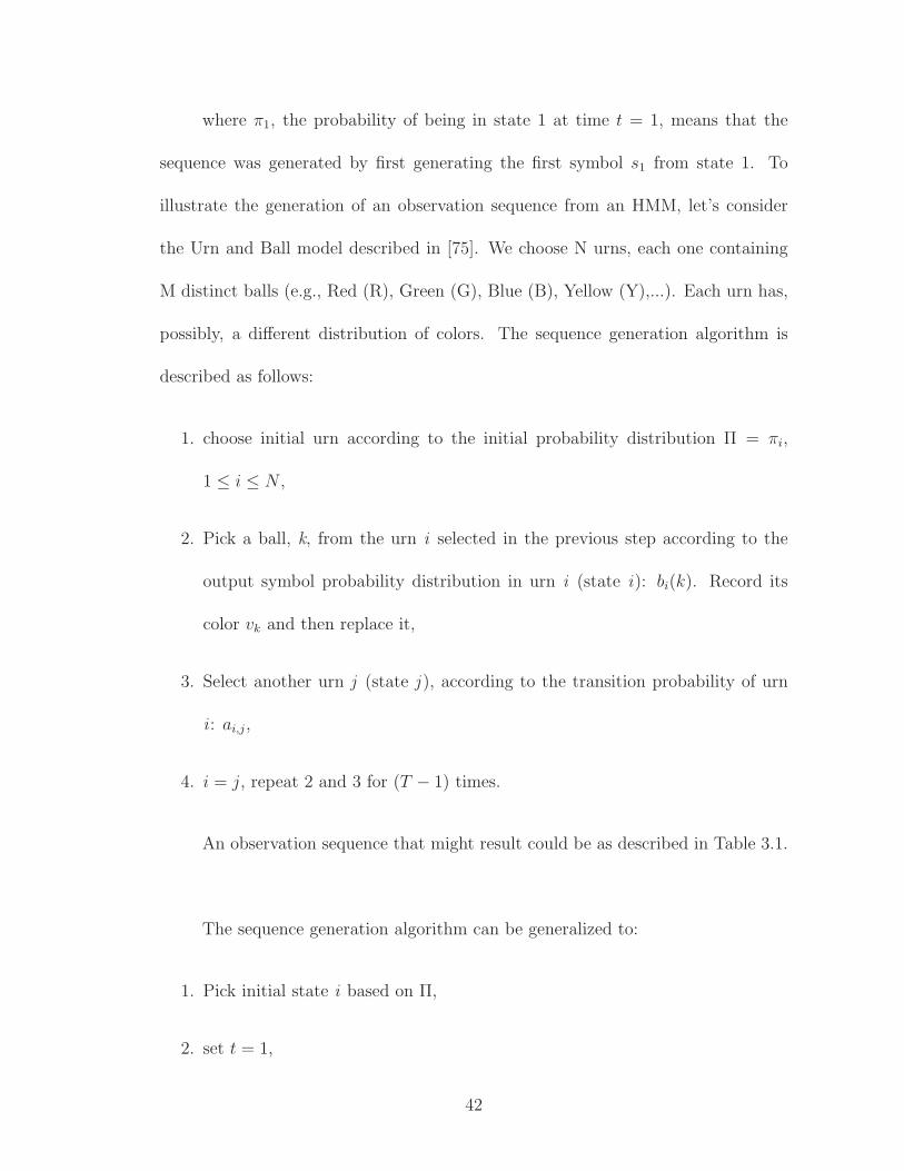
sequence was generated by first generating the first symbol s1 from state 1. To
illustrate the generation of an observation sequence from an HMM, let’s consider
the Urn and Ball model described in [75]. We choose N urns, each one containing
M distinct balls (e.g., Red (R), Green (G), Blue (B), Yellow (Y),...). Each urn has,
possibly, a different distribution of colors. The sequence generation algorithm is
described as follows:
1. choose initial urn according to the initial probability distribution Π = πi,
1 ≤ i ≤ N ,
2. Pick a ball, k, from the urn i selected in the previous step according to the
output symbol probability distribution in urn i (state i): bi(k). Record its
color vk and then replace it,
3. Select another urn j (state j ), according to the transition probability of urn
i : ai,j,
4. i = j, repeat 2 and 3 for (T − 1) times.
An observation sequence that might result could be as described in Table 3.1.
The sequence generation algorithm can be generalized to:
1. Pick initial state i based on Π,
2. set t = 1,
42
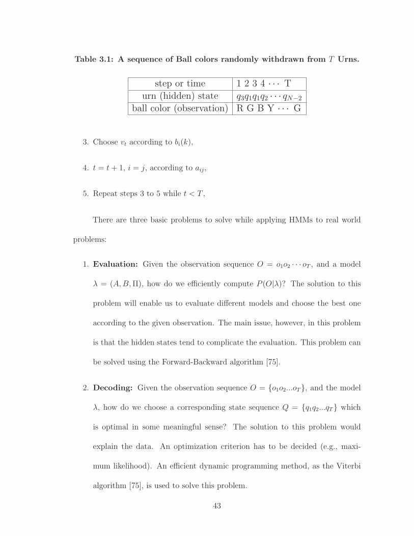
Table 3.1: A sequence of Ball colors randomly withdrawn from T Urns.
step or time 1 2 3 4 · · · T
urn (hidden) state q3q1q1q2 · · · qN−2
ball color (observation) R G B Y · · · G
3. Choose vt according to bi(k),
4. t = t + 1, i = j, according to aij,
5. Repeat steps 3 to 5 while t < T ,
There are three basic problems to solve while applying HMMs to real world
problems:
1. Evaluation: Given the observation sequence O = o1o2 · · · oT , and a model
λ = (A,B, Π), how do we efficiently compute P (O|λ)? The solution to this
problem will enable us to evaluate different models and choose the best one
according to the given observation. The main issue, however, in this problem
is that the hidden states tend to complicate the evaluation. This problem can
be solved using the Forward-Backward algorithm [75].
2. Decoding: Given the observation sequence O = {o1o2...oT}, and the model
λ, how do we choose a corresponding state sequence Q = {q1q2...qT} which
is optimal in some meaningful sense? The solution to this problem would
explain the data. An optimization criterion has to be decided (e.g., maxi-
mum likelihood). An efficient dynamic programming method, as the Viterbi
algorithm [75], is used to solve this problem.
43
3. Learning: How do we adjust the model parameters λ = (A,B, Π) to max-
imize P (O|λ)? This problem is about finding the best model that describes
the observation at hand.
Of all the three problems, the third one is the most crucial and challenging
to solve for most applications of HMMs. The work presented in this thesis mainely
focuses on this problem.
3.2 Estimation of HMM parameters
The parameters estimation problem can be divided into two categories:
1. Structure of the HMM: Define the number of states N , how they are
connected, and the number, M , of output symbols in each state.
2. Parameters value estimation: Estimate the transition probability matrix
A, the emission probabilities B, and the initial probabilities Π.
For both categories we will assume that the data at hand is composed of
example sequences (training sequence), denoted as O = {o1, o2 · · · oT}, that are
independent. Thus:
P (O|λ) =T
∑
t=1
P (ot|λ) (3.4)
Section 3.2.1, will address the theory of parameter estimation problem and
some of the methods that have been developed to solve it. Section 3.2.3 will describe
the topology choice of the HMM that depends heavily on the problem at hand.
44
3.2.1 Estimation of HMM parameters
Due to the complexity of the problem and the finite number of observations,
there is no known analytical method so far for estimating λ to globally maximize
P (O|λ). Instead, iterative methods that provide a local maxima on P (O|λ) can be
used such as the frequently used Baum-Welch estimation algorithm [14]. Besides
the well known Viterbi and Baum-Welch methods [75], in [78], the authors used a
gradient descent method to estimate the HMM parameters, and a back-propagation
neural network to determine the states of the HMM. In [66], associative mining was
used to estimate the parameters of an all Kth-order Prediction-by-Partial-Match
(PPM) Markov Predictors. We will look more closely at this method later on and
compare it to the method we present in this work.
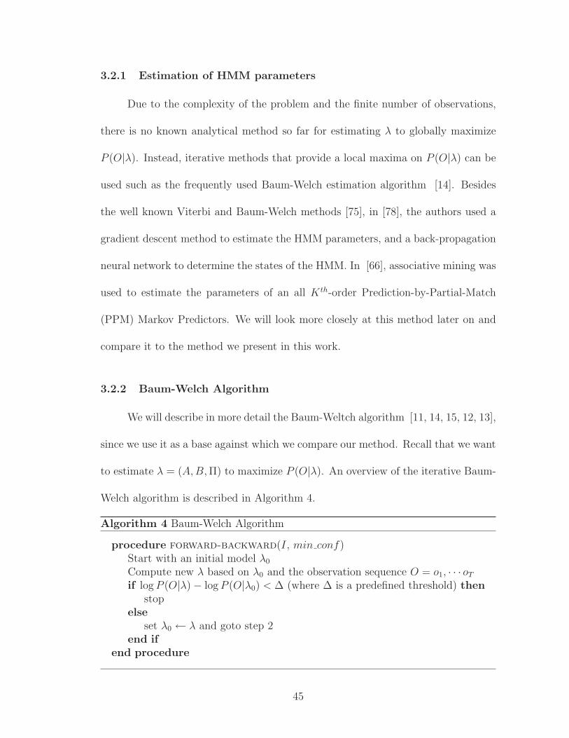
3.2.2 Baum-Welch Algorithm
We will describe in more detail the Baum-Weltch algorithm [11, 14, 15, 12, 13],
since we use it as a base against which we compare our method. Recall that we want
to estimate λ = (A,B, Π) to maximize P (O|λ). An overview of the iterative Baum-
Welch algorithm is described in Algorithm 4.
Algorithm 4 Baum-Welch Algorithm
procedure forward-backward(I, min conf)Start with an initial model λ0
Compute new λ based on λ0 and the observation sequence O = o1, · · · oT
if log P (O|λ) − log P (O|λ0) < ∆ (where ∆ is a predefined threshold) thenstop
elseset λ0 ← λ and goto step 2
end ifend procedure
45
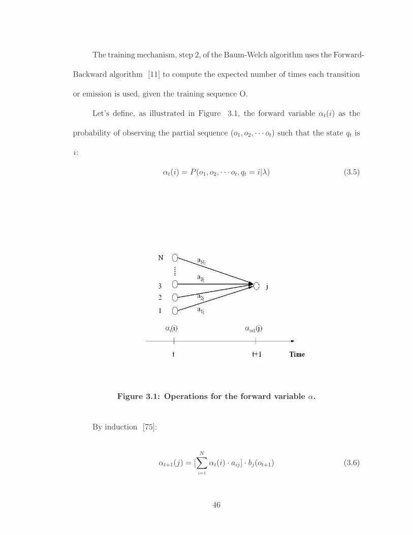
The training mechanism, step 2, of the Baum-Welch algorithm uses the Forward-
Backward algorithm [11] to compute the expected number of times each transition
or emission is used, given the training sequence O.
Let’s define, as illustrated in Figure 3.1, the forward variable αt(i) as the
probability of observing the partial sequence (o1, o2, · · · ot) such that the state qt is
i :
αt(i) = P (o1, o2, · · · ot, qt = i|λ) (3.5)
Figure 3.1: Operations for the forward variable α.
By induction [75]:
αt+1(j) = [N
∑
i=1
αt(i) · aij] · bj(ot+1) (3.6)
46
where, 1 ≤ j ≤ N and 1 ≤ t ≤ T − 1.
With the initial value at t = 1, α1(i) = πibi(ot+1), we obtain:
P (O|λ) =N
∑
i=1
αT (i) (3.7)
This computation is in the order O(N2T ).
Let’s define the backward variable βt(i), shown in Figure 3.2, as the probability
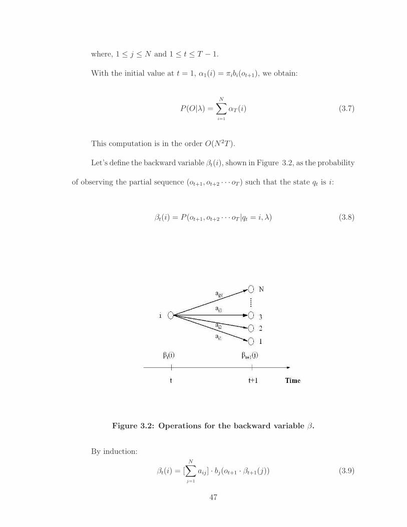
of observing the partial sequence (ot+1, ot+2 · · · oT ) such that the state qt is i :
βt(i) = P (ot+1, ot+2 · · · oT |qt = i, λ) (3.8)
Figure 3.2: Operations for the backward variable β.
By induction:
βt(i) = [N
∑
j=1
aij] · bj(ot+1 · βt+1(j)) (3.9)
47
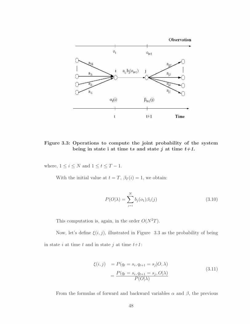
Figure 3.3: Operations to compute the joint probability of the systembeing in state i at time ts and state j at time t+1.
where, 1 ≤ i ≤ N and 1 ≤ t ≤ T − 1.
With the initial value at t = T , βT (i) = 1, we obtain:
P (O|λ) =N
∑
j=1
bj(o1)β1(j) (3.10)
This computation is, again, in the order O(N2T ).
Now, let’s define ξ(i, j), illustrated in Figure 3.3 as the probability of being
in state i at time t and in state j at time t+1 :
ξ(i, j) = P (qt = si, qt+1 = sj|O, λ)
=P (qt = si, qt+1 = sj, O|λ)
P (O|λ)
(3.11)
From the formulas of forward and backward variables α and β, the previous
48
formula can be rewritten as:
ξ(i, j) =αt(i) · aij · bj(vt+1) · βt+1(j)
P (O|λ)
=αt(i) · aij · bj(vt+1) · βt+1(j)
N∑
i=1
N∑
j=1
αt(i) · aij · bj(vt+1) · βt+1(j)
(3.12)
We then define, γt(i) as the probability of being in state i at time t, given the
observation sequence:
γt(i) =N
∑
j=1
ξt(i, j) (3.13)
where:
•T∑
t=1
γt(i) is the expected number of times state i is visited.
•T−1∑
t=1
ξt(i, j) is the expected number of transitions from state i to state j.
The above formulas are used along with the concept of counting event occur-
rences in Baum-Welch algorithm to estimate the elements of the model λ, Π, A, and
B as follows:
• πi = γ1(i), which is the expected frequency in state i at time t = 1.
• aij =
T−1∑
t=1
ξt(i, j)
T−1∑
t=1
γt(i)
, which is (the expected number of transition from state i to
state j )/(expected number of transition from state i).
• bj(k) =
T∑
t=1ot=vk
γt(j)
T∑
t=1
γt(j)
.
49
These values are iteratively computed, and converge in a continuous space
until a converging criteria is met, typically stopping when the difference in the log
of likelihood [log(P (O|λ))− log(P (O|λ0))] is smaller than a predefined threshold ∆
or the maximum number of iterations is reached. At each iteration, the log likelihood
of the model λ is increased, converging the model to a local maximum.
As pointed out in the beginning of this section, in a continuous-valued space
there is no known method to get a global optimum, but rather a local maximum can
be reached. The values of the initial parameters, used in the Baum-Welch algorithm,
influence heavily the local maximum that the model converges to. This becomes a
severe problem when dealing with large scale HMMs, which is the case in most of
real-world applications, if not all of them.
3.2.3 Structure of HMM
In the previous section we explored different methods of estimating the param-
eter values of an HMM. We considered a simplified HMM structure that consists
of N states fully connected. This type of HMM is known as ergodic. Formally
speaking, any state of the HMM could be reached by any other state in one step
(i.e., ai,j 6= 0 for ∀ i, j ∈ {1, · · ·N}). These types of HMMs, even though they seem
simple, are computationally expensive and perform poorly in real world problems.
In fact, even with enough training data to estimate all the parameters, an issue with
this type of HMM structure is still the local maximum problem.
50
3.3 Hidden Markov Models: Related Work
As stated earlier the ergodic HMMs, even though they seem simple, are com-
putationally expensive and perform poorly in real world problems. In fact, even with
enough training data to estimate all the parameters, the problem with this type of
HMM structure will be the local maximum problem. Therefore, a good structure
for the HMM should be constrained. However, how constrained should it be is not
an easy question to solve, since it depends on the problem at hand.
In speech recognition [9, 50], a left-right model was shown to model the
observed properties of the signal that change over time better than the ergodic
HMM. The states proceed from left to right as time increases. An extension of the
left-right model is a cross-coupled connection of two parallel left-right HMMs which
was proposed in [75]. In [41], the HMM topology adapts to the data by adding and
deleting transitions and states. In [57, 77], a non- parametric state duration density
Pi(d) is considered instead of the self-transition coefficient aii. The transition from
state i to state j is made only after the appropriate number of observations are
generated according to Pi(d). However, this method is computationally expensive
and it increases the complexity of the system by increasing the number of parameters
to be estimated. To cope with this drawback, Guassian families with mean and
standard deviation as parameters to be estimated are used as Pi(d) [56], and in [61]
a path-constrained Viterbi decoding method with a unifrom duration distribution
is used.
In speech recognition [75] as well as in biological sequence analysis [27], another
51
type of HMMs is considered where the observations are associated with connections
rather than the states of the model and allowing states to emit no symbols, known
as the Silent or Null states. Another method that has been used to reduce the
complexity of the number of parameters to be estimated, especially when there is
insufficient training data, is parameter Tying [79]. This technique consists of making
up an equivalence relation between the parameters in different states, reducing this
way, the number of independent parameters.
The main problem with HMMs is that they depend on the Markov property,
i.e., the current state depends only on the previous state. In general patterns may
display longer range dependencies, and one needs a higher-order HMM [26] (where
the order denotes the number of previous states the current state depends on) to
model such patterns. Thus, in addition to HMMs (of order 1), there are other
types of Markov models used in prediction. For example, an m−order Prediction-
by-Partial Match (PPM) predictor maintains a Markov model of order j, for all
1 ≤ j ≤ m. This scheme is also referred to as an All-m-Order Markov Model [66].
This model uses the past j events to compute the probability of next event to come.
Mixed-order HMMs have also been proposed [81]. The main challenge here is that
building higher order HMMs [26] is not easy, since we have to estimate the joint
probabilities of the previous m states (in an m-order HMM). Furthermore, not all of
the previous m states may predict the current state. Moreover, the training process
is extremely expensive and suffers from local optima. This leads us to consider a
novel approach of using variable-order HMMs via data mining. The basic idea is
to use data mining to mine frequent patterns, which may be of different lengths,
52

and then use these frequent patterns as the estimates of the joint probabilities,
which can be used to seed the variable-order HMM. There has been almost no
work on variable-order HMMs. The closest work is that of [66], who proposed
using frequent associations for support, confidence and error pruned markov models
(S/C/E-PMMs). However, we plan to use other higher order patterns (sequences)
[98].
In the next section, we describe our proposed Variable Order Gaps state ma-
chine (VOGUE), its parameters and structure estimation via sequence mining using
VGS, described in Chapter 2, as well as some examples to illustrate the method.
Estimating VOGUE’s parameters and structure is deterministic, thanks to the use
of VGS, in contrast to higher-order HMM where the estimation is iterative and
non-deterministic.
3.4 Modeling: Variable-Order State Machine
VOGUE uses the mined sequences to build a variable order/gap state ma-
chine. The main idea here is to model each non-gap symbol in the mined sequences
as a state that emits only that symbol and to add intermediate gap states between
any two non-gap states. The gap states will capture the distribution of the gap
symbols and length. Let F be the set of frequent subsequences mined by VGS, and
let k be the maximum length of any sequence. While VOGUE can be generalized
to use any value of k ≥ 2, for clarity of exposition we will illustrate the working of
VOGUE using mined sequences of length k = 2. We consider the general case in
the next section. Let F1 and F2 be the sets of all frequent sequences of length 1 and
53
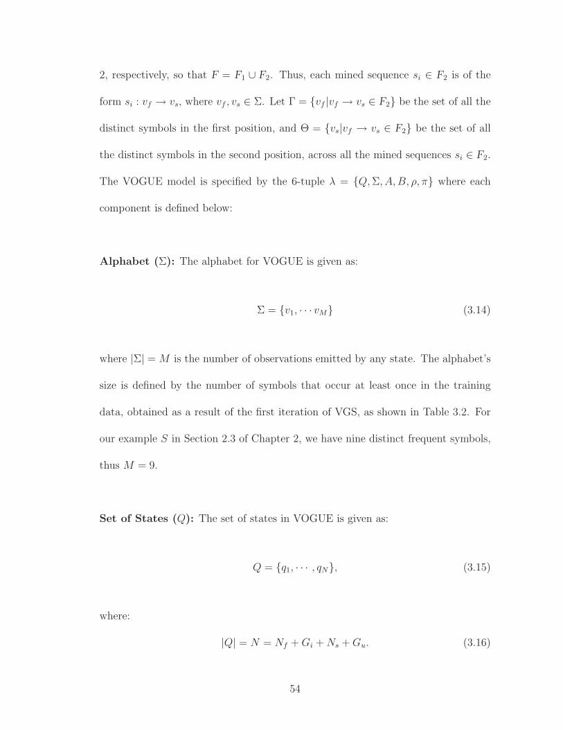
2, respectively, so that F = F1 ∪ F2. Thus, each mined sequence si ∈ F2 is of the
form si : vf → vs, where vf , vs ∈ Σ. Let Γ = {vf |vf → vs ∈ F2} be the set of all the
distinct symbols in the first position, and Θ = {vs|vf → vs ∈ F2} be the set of all
the distinct symbols in the second position, across all the mined sequences si ∈ F2.
The VOGUE model is specified by the 6-tuple λ = {Q, Σ, A,B, ρ, π} where each
component is defined below:
Alphabet (Σ): The alphabet for VOGUE is given as:
Σ = {v1, · · · vM} (3.14)
where |Σ| = M is the number of observations emitted by any state. The alphabet’s
size is defined by the number of symbols that occur at least once in the training
data, obtained as a result of the first iteration of VGS, as shown in Table 3.2. For
our example S in Section 2.3 of Chapter 2, we have nine distinct frequent symbols,
thus M = 9.
Set of States (Q): The set of states in VOGUE is given as:
Q = {q1, · · · , qN}, (3.15)
where:
|Q| = N = Nf + Gi + Ns + Gu. (3.16)
54
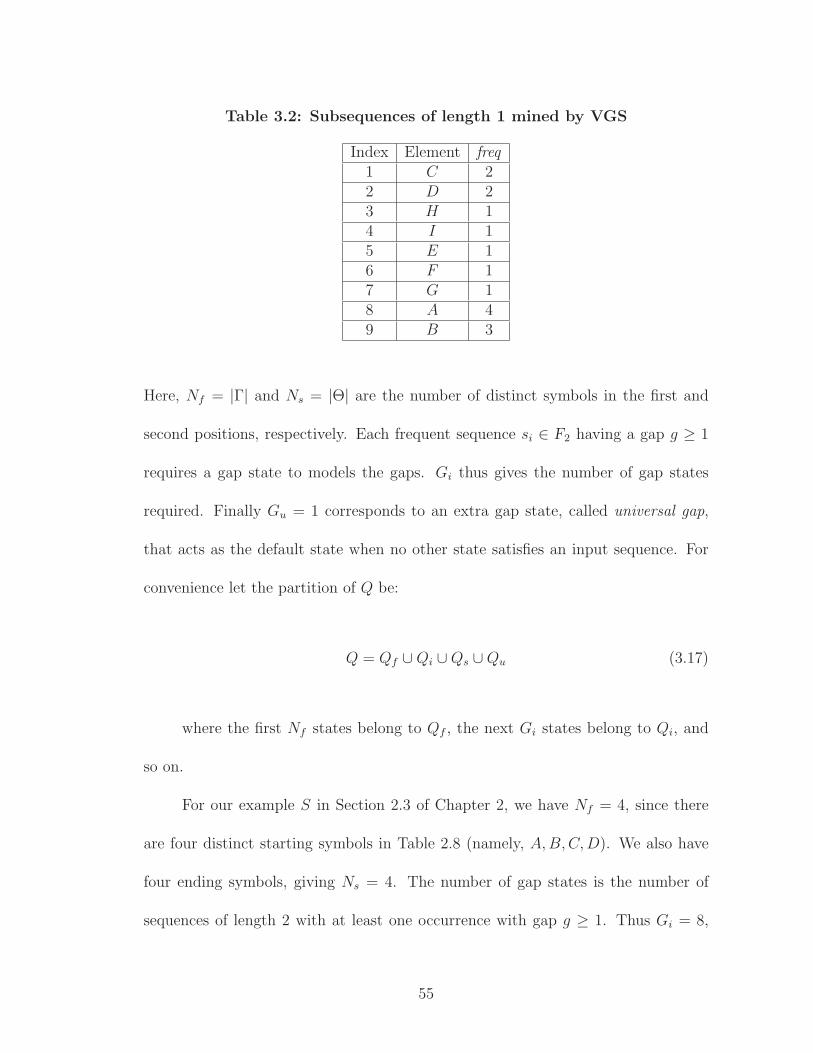
Table 3.2: Subsequences of length 1 mined by VGS
Index Element freq1 C 22 D 23 H 14 I 15 E 16 F 17 G 18 A 49 B 3
Here, Nf = |Γ| and Ns = |Θ| are the number of distinct symbols in the first and
second positions, respectively. Each frequent sequence si ∈ F2 having a gap g ≥ 1
requires a gap state to models the gaps. Gi thus gives the number of gap states
required. Finally Gu = 1 corresponds to an extra gap state, called universal gap,
that acts as the default state when no other state satisfies an input sequence. For
convenience let the partition of Q be:
Q = Qf ∪ Qi ∪ Qs ∪ Qu (3.17)
where the first Nf states belong to Qf , the next Gi states belong to Qi, and
so on.
For our example S in Section 2.3 of Chapter 2, we have Nf = 4, since there
are four distinct starting symbols in Table 2.8 (namely, A,B,C,D). We also have
four ending symbols, giving Ns = 4. The number of gap states is the number of
sequences of length 2 with at least one occurrence with gap g ≥ 1. Thus Gi = 8,
55
C → B is the only sequence that has all consecutive (g = 0) occurrences. With one
universal gap state Gu = 1, our model yields N = 4 + 8 + 4 + 1 = 17 states.
Transition Probability Matrix (A): The transition probability matrix between
the states:
A = {a(qi, qj)|1 ≤ i, j ≤ N} (3.18)
where:
a(qi, qj) = P (qt+1 = qj|qt = qi) (3.19)
gives the probability of moving from state qi to qj (where t is the current position
in the sequence). The probabilities depend on the types of states involved in the
transitions. The basic intuition is to allow transitions from the first symbol states
to either the gap states or the second symbol states. The second symbol states
can go back to either the first symbol states or to the universal gap state. Finally
the universal gap state can go to any of the starting states or the intermediate gap
states. We discuss these cases below.
• Transitions from First States: Any first symbol state qi ∈ Qf may tran-
sition to either a second symbol state qj ∈ Qs (modeling a gap of g = 0) or to
a gap state qj ∈ Qi (modeling a gap of g ∈ [1,maxgap]). Let siy : vi → vy ∈ F2
be a subsequence mined by VGS. Let freqgi (y) denote the frequency of siy for a
given gap value g, and let freqi(y) denote the total frequency of the sequence,
56
i.e.:
freqi(y) =
maxgap∑
g=0
freqgi (y) (3.20)
Let the fraction of gap-less transitions from qi to qj over all the transitions
from qi to qy ∈ Qs be denoted as:
R =freq0
i (j)∑
y∈Qs
freqi(y)(3.21)
The transition probabilities from qi ∈ Qf are given as:
a(qi, qj) =
R, qj ∈ Qs
freqi(j)∑
y∈Qs
freqi(y)− R, qj ∈ Qi
0, qj ∈ Qf ∪ Qu
(3.22)
• Transitions from Gap States: Any gap state qi ∈ Qi may only transition
to second symbol state qj ∈ Qs. For qi ∈ Qi we have:
a(qi, qj) =
1, qj ∈ Qs
0, otherwise
(3.23)
• Transitions from Second States: A second symbol state qi ∈ Qs may
transition to either first symbol state qj ∈ Qf (modeling a gap of g = 0),
or to the universal gap state qj ∈ Qu (modeling other gaps). Let T =
∑
sx∈F2freq(sx) be the sum of frequencies of all the sequences in F2. For
57
qi ∈ Qs we have:
a(qi, qj) =
0.99 ×
∑
qy∈Qf
freqj(y)
T , qj ∈ Qf
0.01, qj ∈ Qu
0, qj ∈ Qi ∪ Qs
(3.24)
Transitions back to first states are independent of qi, i.e., the same for all qi ∈
Qs. In fact, these transitions are the same as the initialization probabilities
described below. They allow the model to loop back after modeling a frequent
sequence. Note, that we are primarily modeling the frequent sequences mined
by VGS. However, we need to account for symbols that may appear between
the frequent sequences but are not picked up as frequent. In a statistical model
such as HMM, if a position or a subsequence of positions in an observation
sequence is not present, then the probability of the sequence with respect to
the model will be very small, regardless of how well it may match the rest of
the model.
For example, assume a model built on two frequent subsequences A → B and
C → D. The sequence S ′ = ABRCD should be clearly identified to be a
good match to the model since both subsequences A → B and C → D are
present in it. However, after being in the state that will generate the symbol
B we need to generate the symbol R that is not in any of the two frequent
sequences. Therefore, we need a transition to the universal gap state. However,
since R → B was not identified as being frequent by VGS we need to assign a
58
small probability to this transition. Therefore, we assign an empirically chosen
value of 1% to the transition from the “second states” to the universal gap
state. Furthermore, sinceN∑
j=1
a(qi, qj) = 1 we assign the remaining 99% to the
transition to the “first states”.
• Transitions from Universal Gap: The universal gap state can only tran-
sition to the first states or the intermediate gap states. For qi ∈ Qu we have:
a(qi, qj) =
0.9 ×
∑
qy∈Qf
freqj(y)
T , qj ∈ Qf
0.1 × 1Gi
, qj ∈ Qi
0, otherwise
(3.25)
Since the first states can emit only one symbol, we allow transitions from
universal gap to intermediate gap states, to allow for other symbol emissions.
For example, assuming, as before, the same frequent sequences are A → B
and C → D that are used to build the model. If we have a new observation
sequence S ′′ = ABRFCD, clearly we need to generate two symbols, R and F ,
between the two frequent sequences A → B and C → D. After generating B
from a second state, we can generate R from the universal gap state however we
need to generate one more symbol, F . F does not belong to any of the frequent
sequence before generating the other frequent sequence C → D. Therefore
there is a need to transit from the gap state to an intermediate gap state since
the first and second symbols can only generate symbols that belong to the
frequent sequences. Moreover, since generating F after R was not identified
59
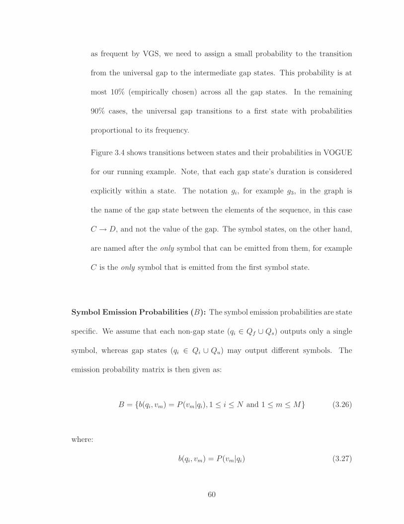
as frequent by VGS, we need to assign a small probability to the transition
from the universal gap to the intermediate gap states. This probability is at
most 10% (empirically chosen) across all the gap states. In the remaining
90% cases, the universal gap transitions to a first state with probabilities
proportional to its frequency.
Figure 3.4 shows transitions between states and their probabilities in VOGUE
for our running example. Note, that each gap state’s duration is considered
explicitly within a state. The notation gi, for example g3, in the graph is
the name of the gap state between the elements of the sequence, in this case
C → D, and not the value of the gap. The symbol states, on the other hand,
are named after the only symbol that can be emitted from them, for example
C is the only symbol that is emitted from the first symbol state.
Symbol Emission Probabilities (B): The symbol emission probabilities are state
specific. We assume that each non-gap state (qi ∈ Qf ∪ Qs) outputs only a single
symbol, whereas gap states (qi ∈ Qi ∪ Qu) may output different symbols. The
emission probability matrix is then given as:
B = {b(qi, vm) = P (vm|qi), 1 ≤ i ≤ N and 1 ≤ m ≤ M} (3.26)
where:
b(qi, vm) = P (vm|qi) (3.27)
60
g1
C
0.31
A
0.36
D
0.1
B
0.21
g2
0.012
g3
0.012
g4
0.012
g5
0.012
g6
0.012
g7
0.012
g8
0.012
g9
0.012
B
0.33
0.33 0.33
D
0.14
C
0.14
0.42 0.14 0.14
A
0.5
0.5
0.25 0.25
0.25 0.25 0.01
0.31 0.36 0.1 0.2
0.01
0.31 0.1 0.360.2
0.01
0.31 0.1 0.36 0.2
0.01
0.31 0.1 0.360.2
1 1 1 1 1 1 1 1
Figure 3.4: VOGUE State Machine for Running Example
61
is the probability of emitting symbol vm in state qi. b(qi, vm) differs depending
on whether qi is a gap state or not. Since there is a chance that some symbols that
do not occur in the training data may in fact be present in the testing data, we
assign them a very small probability of emission in the gap states.
• Non-gap States: the emission probability is:
b(qi, vm) =
1, qi ∈ Qf ∪ Qs
0, otherwise
(3.28)
For example, the first and second states are labeled by their emission symbol
in Figure 3.4.
• Universal Gap: For qi ∈ Qu we have:
b(qi, vm) =
freqi(vm)∑
vm∈Σ
freqi(vm)
× 0.99 + c′ (3.29)
where c′ = 0.01M .
This means that vm is emitted with probability proportional to its frequency
in the training data. The c′ term handles the case when vm does not appear
in the training set.
• Gap States: If qi ∈ Qi its emission probability depends on the symbol
distribution mined by VGS. Let Σqibe the set of symbols that were observed
62
by VGS in the gap qi. We have:
b(qi, vm) =
∑
g≥1
freqg(vm, qi)
∑
vm∈Σqi
∑
g≥1
freqg(vm, qi)
× 0.99 + c (3.30)
where c = 0.01|Σqi
|.
Note that the above summations are for gap ranges g ∈ [1,maxgap], since gap g = 0
is treated as a direct transition from one state to another. Note that the values 0.99
and 0.01 above arise from the pseudo-count approach used for previously unseen
symbols.
In our running example, for the symbol vm = C and the gap state g4 between
the states that emit A and B, we have the frequency of C as 2 out of the total
number (5) of symbols seen in the gaps (see Section 2.3 of Chapter 2). Thus C’s
emission probability is 25 × 0.99 + 0.01
4 = 0.385.
Gap Duration Probabilities (ρ): The probability of generating a given number
of gaps from the gap states Qi is given by the gap duration probability matrix:
ρ = {ρ(qi, g)|qi ∈ Qi, g ∈ [1,maxgap]} (3.31)
Let qi be the gap state between a state qx ∈ Qf and a state qy ∈ Qs corresponding
to the sequence s : vi → vy ∈ F2. The gap duration probability is proportional to
63
the frequency of observing a given gap value for s, i.e.:
ρ(qi, g) =
freqgi (y)
∑
g∈{1,··· ,maxgap}
freqgi (y)
, qi ∈ Qi
1, qi ∈ Q\Qi.
(3.32)
In our running example, for the gap state g4 between the states that emit A and
B, we have ρ(g4, 2) = 23 = 0.67, since we observe twice a gap of 2, out of three
occurrences.
Initial State Probabilities (π): The probability of being in state qi initially is
given by π = {π(i) = P (qi|t = 0), 1 ≤ i ≤ N}, where:
π(i) =
0.99 ×
∑
qy∈Qf
freqi(y)
T , qi ∈ Qf
0.01, qi ∈ Qu
0, qi ∈ Qi ∪ Qs
(3.33)
We use a small value for the Universal Gap state as opposed to the states in Qf to
accentuate the patterns retained by VGS while still providing a possibility for gaps
after and before them.
Note that the values 0.99, 0.1, 0.01, etc., used in the transition and emission
probabilities, are obtained by using pseudo-counts [18] to allow for symbols that are
unseen in the training data set.
64
3.5 Generalization of VOGUE to k ≥ 2
Here, we generalize the model to k ≥ 2. Let S be the set of subsequences
mined by VGS, and let k be the maximum length of any sequence. We denote by
k seq a sequence of length k, such as vi1 , vi2 , · · · , vik . Let Γk(j) be the set of symbols
in the jth position in all subsequences s, s ∈ S, of length up to k, j = 1, · · · , k − 1;
Γk(k) is then the set of different last symbols in all subsequences of length up to k.
Finally, let S(j) be the set of subsequences in S of length at least j.
The VOGUE’s state machine is denoted as λ and is made up of the 6-tuple
λ = {Q, V,A,B, ρ, π} where each component is defined as follows:
• Q = {q1, · · · , qN} – the set of states of VOGUE, where N is the number of
states of VOGUE such that: N = N1 +G1 + · · ·+Ni−1 +Gi−1 + · · ·+Nk +Gk,
where:
– Ni =| Γk(i) | , i = 2, · · · , k − 1. This denotes the number of distinct
symbols in position i over all the sequences. Thus N1 is the number of
distinct first symbols and Nk is the number of distinct last symbols.
– Gi (for i < k) is the number of distinct pairs of symbols in positions i−1
and i. This corresponds to the number of gap states required between
states at positions i − 1 and i.
– Gk = 1, corresponds to an extra gap state, called Universal Gap state,
that will capture elements not captured by any of the above.
For convenience we let:
65
–∑
(Gj) =∑
l<j(Nl + Gl) for all j ∈ {2, · · · , k} and∑
(G1) = 0.
–∑
(Nj) =∑
l<j(Gj) + Nj for all j ∈ {1, · · · , k}.
The states of VOGUE are, then, given as follows:
– For∑
(Nj) < i ≤∑
(Gj+1), qi corresponds to the gap of variable length
between the (j−1)th and jth elements in the subsequences, j ∈ {1, · · · , k−
1}. These states will be called “Gap” states.
– For∑
(Gj) < i ≤∑
(Nj), qi corresponds to the elements in Γk(j), j ∈
{1, · · · , k}. These states will be called “Symbol” states.
– For i =∑
(Gk+1), qi corresponds to the Universal Gap state.
• V = {v1, · · · vM} – the alphabet of the symbols, where M is the number of
observations emitted by a state in Q. It is the number of different subsequences
of length 1 retained by VGS, unless stated differently by the application at
hand.
• A = {ail} – the transition probability matrix between the states in Q. For
convenience we let:
– Rsj(m): frequency of subsequence s, s ∈ S, where m is the index of the
symbol vm ∈ Γk(j) at the jth position of s.
– Wjg(m,m′): frequency of subsequence s, s ∈ S, where m and m′ are,
respectively, the indexes of vm and vm′ . vm is at the jth position of s and
vm′ is at the j + 1th position of s. g is the value of the gap between the
jth and j + 1th positions of s, g ∈ {1, · · · ,maxgap}.
66
Each element of the matrix is given as ail = P (qt+1 = l|qt = i), for 1 ≤ i, l ≤ N .
– if∑
(Gj) < i ≤∑
(Nj), j ∈ {1, · · · , k − 1}, (Non-Gap (Symbol) states):
ail =
Pmaxgapg=1 Wjg(m,m′)
P
s∈S Rsj(m), if
∑
(Nj < l ≤∑
(Gj+1));
Wj0(m,m′)P
s∈S Rsj(m), if
∑
(Gj+1) < l ≤∑
(Nj+1);
0, Otherwise;
(3.34)
where m and m′ are the indexes, respectively, of symbols vm and vm′ ∈ V
such that ∃vl′ ∈ Γk(j) and ∃vl” ∈ Γk(j + 1): (vl′ = vm and vl” = vm′),
and (l′ = i −∑
(Gj) and l” = l −∑
(Gj+1)).
– if∑
(Nj) < i ≤∑
(Gj+1), j ∈ {1, · · · , k − 1}, (Gap states):
ail =
0.9, if∑
(Gi+1) < l ≤∑
(Ni+1);
0.1N1+1
if∑
(Nk) < l ≤∑
(Gk+1)
0.1N1+1
if∑
(G1) < l ≤∑
(N1)
0, Otherwise;
(3.35)
– if∑
(Gk) < i ≤∑
(Nk) (last Symbol states):
67
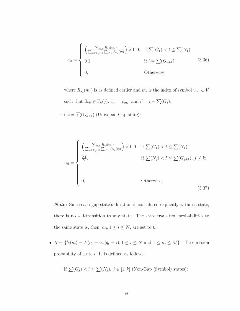
ail =
(P
s∈S Rsj(mi)P
m∈Γk(j)
P
s∈S Rsj(m)
)
× 0.9, if∑
(G1) < l ≤∑
(N1);
0.1, if l =∑
(Gk+1);
0, Otherwise;
(3.36)
where Rsj(mi) is as defined earlier and mi is the index of symbol vmi∈ V
such that ∃vl′ ∈ Γk(j): vl′ = vmi, and l′ = i −
∑
(Gj).
– if i =∑
(Gk+1) (Universal Gap state):
ail =
(P
s∈S Rsj(mi)P
m∈Γk(j)
P
s∈S Rsj(m)
)
× 0.9, if∑
(G1) < l ≤∑
(N1);
0.1G
, if∑
(Nj) < l ≤∑
(Gj+1), j 6= k;
0, Otherwise;
(3.37)
Note: Since each gap state’s duration is considered explicitly within a state,
there is no self-transition to any state. The state transition probabilities to
the same state is, then, aii, 1 ≤ i ≤ N , are set to 0.
• B = {bi(m) = P (ot = vm|qt = i), 1 ≤ i ≤ N and 1 ≤ m ≤ M} - the emission
probability of state i. It is defined as follows:
– if∑
(Gj) < i ≤∑
(Nj), j ∈ [1, k] (Non-Gap (Symbol) states):
68
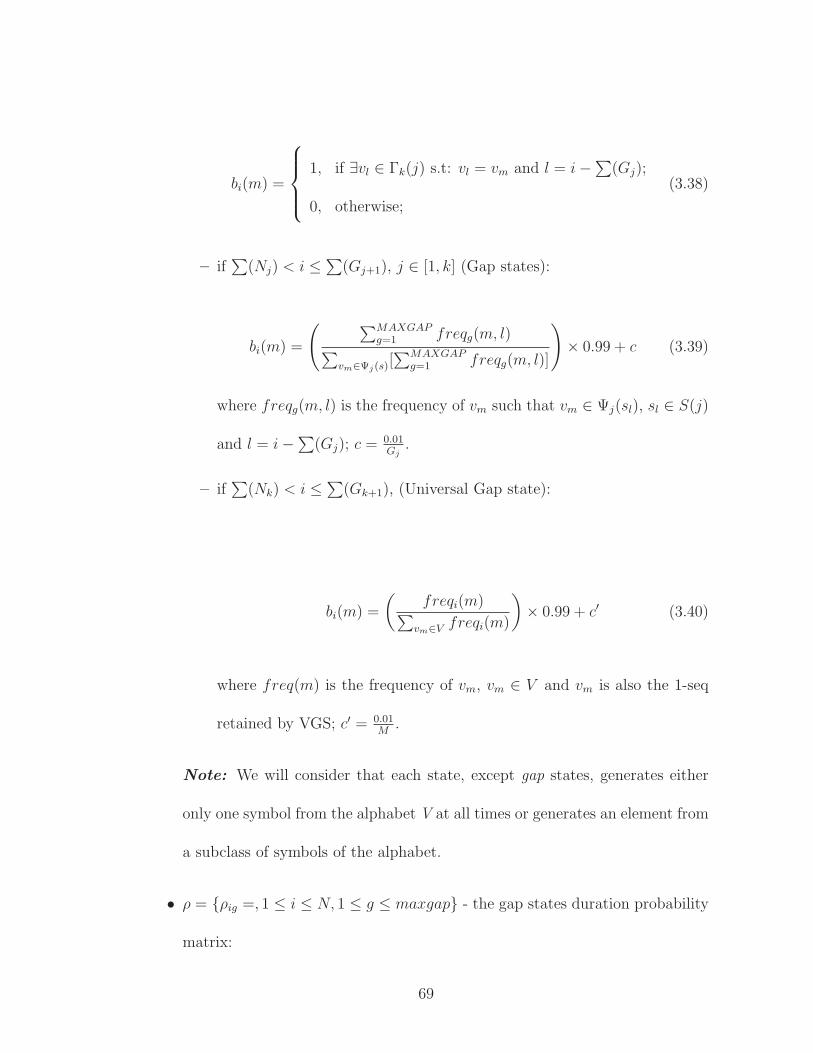
bi(m) =
1, if ∃vl ∈ Γk(j) s.t: vl = vm and l = i −∑
(Gj);
0, otherwise;
(3.38)
– if∑
(Nj) < i ≤∑
(Gj+1), j ∈ [1, k] (Gap states):
bi(m) =
(
∑MAXGAPg=1 freqg(m, l)
∑
vm∈Ψj(s)[∑MAXGAP
g=1 freqg(m, l)]
)
× 0.99 + c (3.39)
where freqg(m, l) is the frequency of vm such that vm ∈ Ψj(sl), sl ∈ S(j)
and l = i −∑
(Gj); c = 0.01Gj
.
– if∑
(Nk) < i ≤∑
(Gk+1), (Universal Gap state):
bi(m) =
(
freqi(m)∑
vm∈V freqi(m)
)
× 0.99 + c′ (3.40)
where freq(m) is the frequency of vm, vm ∈ V and vm is also the 1-seq
retained by VGS; c′ = 0.01M
.
Note: We will consider that each state, except gap states, generates either
only one symbol from the alphabet V at all times or generates an element from
a subclass of symbols of the alphabet.
• ρ = {ρig =, 1 ≤ i ≤ N, 1 ≤ g ≤ maxgap} - the gap states duration probability
matrix:
69
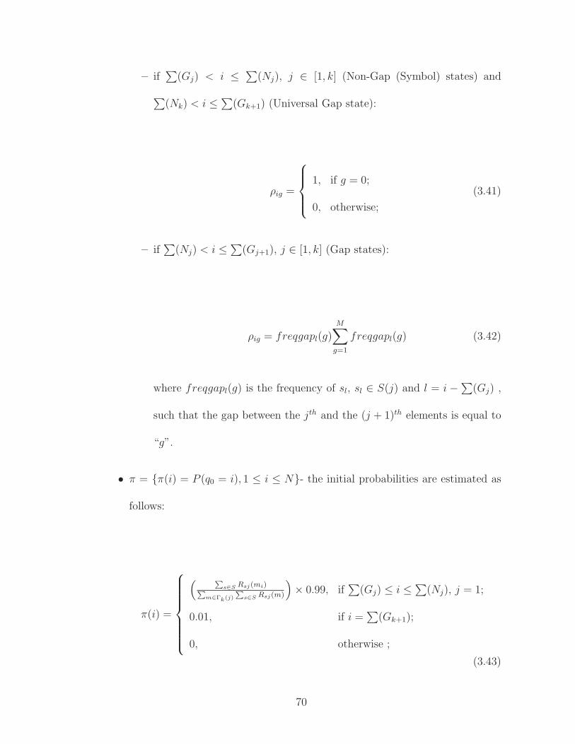
– if∑
(Gj) < i ≤∑
(Nj), j ∈ [1, k] (Non-Gap (Symbol) states) and
∑
(Nk) < i ≤∑
(Gk+1) (Universal Gap state):
ρig =
1, if g = 0;
0, otherwise;
(3.41)
– if∑
(Nj) < i ≤∑
(Gj+1), j ∈ [1, k] (Gap states):
ρig = freqgapl(g)M
∑
g=1
freqgapl(g) (3.42)
where freqgapl(g) is the frequency of sl, sl ∈ S(j) and l = i −∑
(Gj) ,
such that the gap between the jth and the (j + 1)th elements is equal to
“g”.
• π = {π(i) = P (q0 = i), 1 ≤ i ≤ N}- the initial probabilities are estimated as
follows:
π(i) =
(P
s∈S Rsj(mi)P
m∈Γk(j)
P
s∈S Rsj(m)
)
× 0.99, if∑
(Gj) ≤ i ≤∑
(Nj), j = 1;
0.01, if i =∑
(Gk+1);
0, otherwise ;
(3.43)
70
where Rsj(m) is as defined earlier and mi is the index of symbol vmi∈ V such
that ∃vl′ ∈ Γk(j): vl′ = vmi, and l′ = i −
∑
(Gj)..
3.6 Summary
In this Chapter, we described the “modeling” step of VOGUE by introducing
a new variable Order-Gap state machine. In this step VOGUE models each non-
gap symbol in the mined sequences by VGS as a state that emits only that symbol.
Then intermediate states, called gap states, are added between any two gap states to
model the gap between the elements of the frequent sequences mined by VGS. The
gap states capture the distribution of the gap symbols and length. Although other
methods such as Hidden Markov Model (HMM) [58] are good data modeling tools,
VOGUE’s state machine has several differences. HMM parameters are estimated
using an Expectation Maximization method (Baum-Welch) [58], an iterative method
that suffers from local optimum problem, and its structure is estimated on trial and
error basis. On the other hand, VOGUE’s state machine parameters and structure
are estimated deterministically using the frequent sequences mined by VGS and the
distribution and length of the gaps between the elements of those sequences. This
insures a good coverage of the most frequent patterns and a reduced state space
complexity. We substantiate these claims, in Chapter 6, through real data sets
experimentation by comparing the accuracy, coverage and state space complexity of
variable order-gap state machine as opposed to several Hidden Markov Models. In
the next Chapter, we describe two extensions of VOGUE C-VOGUE and K-VOGUE
before describing in Chapter 5 how data “interpretation” is tackled by the VOGUE
71

methodology.
72
Chapter 4VOGUE Variations
In this chapter we describe two variations of VOGUE, namely, Canonical VOGUE
(C-VOGUE), and Knowledge VOGUE (K-VOGUE). C-VOGUE intends to de-
crease even more the state space complexity by pruning frequent sequences mined
by VGS that are artifacts of other “primary” frequent sequences, thus, pruning the
states and transitions from and to those states. Therefore further decreases the
state space complexity. On the other hand, in some domains, such as in biological
sequence analysis, the patterns that are supposed to be frequent do not have an
exact match in all the sequences in the original data set. In fact, some elements of
these patterns could be different, however, they share some common characteristics
and thus called “similar”. Therefore, the sequences in the data set that have a
sequence of elements that are not similar but share some common characteristics
could be incorporated into the model. K-VOGUE is an extension of VOGUE that
takes into consideration these constraints.
73
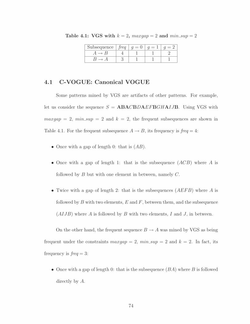
Table 4.1: VGS with k = 2, maxgap = 2 and min sup = 2
Subsequence freq g = 0 g = 1 g = 2A → B 4 1 1 2B → A 3 1 1 1
4.1 C-VOGUE: Canonical VOGUE
Some patterns mined by VGS are artifacts of other patterns. For example,
let us consider the sequence S = ABACBDAEFBGHAIJB. Using VGS with
maxgap = 2, min sup = 2 and k = 2, the frequent subsequences are shown in
Table 4.1. For the frequent subsequence A → B, its frequency is freq = 4:
• Once with a gap of length 0: that is (AB).
• Once with a gap of length 1: that is the subsequence (ACB) where A is
followed by B but with one element in between, namely C.
• Twice with a gap of length 2: that is the subsequences (AEFB) where A is
followed by B with two elements, E and F , between them, and the subsequence
(AIJB) where A is followed by B with two elements, I and J , in between.
On the other hand, the frequent sequence B → A was mined by VGS as being
frequent under the constraints maxgap = 2, min sup = 2 and k = 2. In fact, its
frequency is freq = 3:
• Once with a gap of length 0: that is the subsequence (BA) where B is followed
directly by A.
74
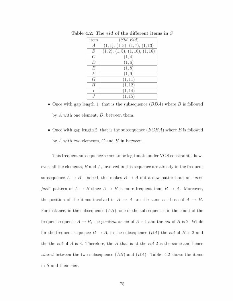
Table 4.2: The eid of the different items in S
item (Sid, Eid)A (1, 1), (1, 3), (1, 7), (1, 13)B (1, 2), (1, 5), (1, 10), (1, 16)C (1, 4)D (1, 6)E (1, 8)F (1, 9)G (1, 11)H (1, 12)I (1, 14)J (1, 15)
• Once with gap length 1: that is the subsequence (BDA) where B is followed
by A with one element, D, between them.
• Once with gap length 2, that is the subsequence (BGHA) where B is followed
by A with two elements, G and H in between.
This frequent subsequence seems to be legitimate under VGS constraints, how-
ever, all the elements, B and A, involved in this sequence are already in the frequent
subsequence A → B. Indeed, this makes B → A not a new pattern but an “arti-
fact” pattern of A → B since A → B is more frequent than B → A. Moreover,
the position of the items involved in B → A are the same as those of A → B.
For instance, in the subsequence (AB), one of the subsequences in the count of the
frequent sequence A → B, the position or eid of A is 1 and the eid of B is 2. While
for the frequent sequence B → A, in the subsequence (BA) the eid of B is 2 and
the the eid of A is 3. Therefore, the B that is at the eid 2 is the same and hence
shared between the two subsequence (AB) and (BA). Table 4.2 shows the items
in S and their eids.
75
The items in S that are shared between A → B and B → A in the for-
mat of (items, eid) are {(B, 2), (A, 3), (B, 5), (A, 7), (B, 10), (A, 13)}. Therefore, the
subsequence (BA) is an artifact of (AB) and (ACB). The subsequence (BDA) is
an artifact of (ACB) and (AEFB). The subsequence (BGHA) is an artifact of
(AEFB) and (AIJB). Hence, the frequent subsequence B → A is an “artifact”
pattern of the “primary” pattern A → B.
Figure 4.1 shows the structure of VOGUE State Machine with N = 7 being
the number of states for our example sequence. In fact, Nf = 2 since there are 2
distinct starting symbols in Table 4.1 (namely A and B). We also have 2 ending
symbols giving (namely A and B)Ns = 2. The number of gap states is the number of
sequences of length 2 that has at least one occurrence with gap g ≥ 1, thus, Gi = 2.
Since we have one universal gap Gu = 1, our model yields N = Nf +Gi +Ns +Gu =
2 + 2 + 2 + 1 = 7. We can see clearly that the paths A → B and B → A can
be merged into one path A → B and the information of gap g2 and g3 can be also
contained in one gap state instead of two. In fact, for our example, by eliminating
B → A, and hence the states associated with the path B → A from the frequent
mined sequences to build the Variable-Order state machine the number of states
drops from N = 7 to N = 4. By doing so, we reduce the state space complexity
significantly while conserving the coverage and accuracy as we will show through
experimental results in Chapter 6.
After showing the benefits of pruning the states associated with the artifact
patterns, we need a special pruning mechanism to separate primary patterns from
artifact patterns.
76
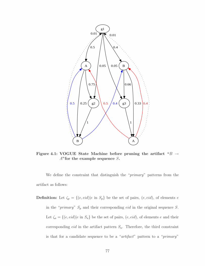
g1
A
0.5
B
0.4
g2
0.05
g3
0.05
B
0.25
0.75
A
0.33
0.66
0.01
0.5 0.4
0.01
0.5 0.4
1 1
Figure 4.1: VOGUE State Machine before pruning the artifact “B →A”for the example sequence S.
We define the constraint that distinguish the “primary” patterns from the
artifact as follows:
Definition: Let ζp = {(e, eid)|e in Sp} be the set of pairs, (e, eid), of elements e
in the “primary” Sp and their corresponding eid in the original sequence S.
Let ζa = {(e, eid)|e in Sa} be the set of pairs, (e, eid), of elements e and their
corresponding eid in the artifact pattern Sa. Therefore, the third constraint
is that for a candidate sequence to be a “artifact” pattern to a “primary”
77
pattern the following conditions have to be satisfied as well:
1. ζa ⊂ ζp.
2. ∃ (e′, eid′), (e′′, eid′′) ∈ ζp such that eid′ < eid < eid′′, where (e, eid) ∈ ζa.
This constraint is necessary.
As consequence of this constraint we have the following condition:
Condition 1: The artifact patterns are less frequent than the corresponding pri-
mary ones. In fact, for our running example, the frequency of the primary
pattern A → B is freq = 4, while the frequency of the artifact pattern B → A
is freq = 3.
In the case of when the mined patterns by VGS are of length k = 2, the following
condition is a consequence of the constraint of artifact patterns:
Condition 2: The elements of the primary and the artifact patterns are “mir-
rored”. In fact, let α → β be the primary pattern and κ → ν be the artifact
pattern. On one hand, the first element, κ, in the artifact pattern is the same
as the second last element, β, in the corresponding primary pattern (κ = β).
On the other hand, the last element,ν, of the artifact pattern is the same as
the first element, α, in the corresponding primary pattern (α = ν). In fact,
in our running example, the first element of the artifact pattern B → A is
B, which is the last element in the corresponding primary pattern A → B.
Likewise, the last element of the artifact pattern B → A is A, which is the
first element of the primary pattern A → B. Therefore, we consider that the
78
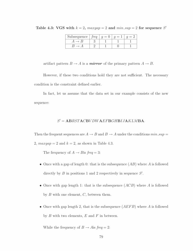
Table 4.3: VGS with k = 2, maxgap = 2 and min sup = 2 for sequence S ′
Subsequence freq g = 0 g = 1 g = 2A → B 3 1 1 1B → A 2 1 0 1
artifact pattern B → A is a mirror of the primary pattern A → B.
However, if these two conditions hold they are not sufficient. The necessary
condition is the constraint defined earlier.
In fact, let us assume that the data set in our example consists of the new
sequence:
S ′ = ABRSTACBV DWAEFBGHBIJAKLMBA.
Then the frequent sequences are A → B and B → A under the conditions min sup =
2, maxgap = 2 and k = 2, as shown in Table 4.3.
The frequency of A → Bis freq = 3:
• Once with a gap of length 0: that is the subsequence (AB) where A is followed
directly by B in positions 1 and 2 respectively in sequence S ′.
• Once with gap length 1: that is the subsequence (ACB) where A is followed
by B with one element, C, between them.
• Once with gap length 2, that is the subsequence (AEFB) where A is followed
by B with two elements, E and F in between.
While the frequency of B → Ais freq = 2:
79
• Once with a gap of length 0: that is the subsequence (BA) where B is followed
directly by A in the positions 25, 26 respectively.
• Once with gap length 2: that is the subsequence (BGHA) where B is followed
by A with two elements, G and H, between them.
Although B → A is a mirror of A → B and the frequency of B → A is
freq = 2 which is less than the one of A → B (freq = 3), B → A cannot be considered
an artifacts pattern of A → B. This is because the positions or eid of the elements
A and B in A → B are different and far from those in B → A. Therefore, B → A
is not in the span of A → B or vice versa. Indeed, as shown in Table 4.4, the
elements A and B in A → B (ζp = {(A, 1), (A, 6), (A, 12), (B, 2), (B, 8), (B, 15)})
all have eids that are different and less in value than the ones in B → A (ζa =
{(A, 21), (A, 26), (B, 18), (B, 25)}). Note that we are considering patterns with a
maxgap = 2 that is why (A, 21) (B, 25) are not in ζA→B because in this case A is
followed by B with 3 elements in between. Therefore, the two sequences are not
interleaved. On the other hand, as shown in Table 4.2 for the example sequence S,
the set ζa of the pairs of elements and their eids of B → A is:
ζa = {(A, 3), (A, 7), (A, 13), (B, 2), (B, 5), (B, 10)}
and the one of A → B is:
ζp = {(A, 1), (A, 3), (A, 7), (A, 13), (B, 2), (B, 5), (B, 10), (B, 16)}
80

. We see clearly that ζa ⊂ ζp. Moreover, B in A → B has an eid that is greater
than any ones identified in ζa, that is (B, 16). Likewise, the element A has an extra
eid in A → B, which corresponds to (A, 1) the smallest eid value in S.
Table 4.4: The eid of the different items in S ′
item (sid, eid)A (1, 1), (1, 6), (1, 12), (1, 21), (1, 26)B (1, 2), (1, 8), (1, 15), (1, 18), (1, 25)C (1, 7)D (1, 10)E (1, 13)F (1, 14)G (1, 16)H (1, 17)I (1, 19)J (1, 20)K (1, 22)L (1, 23)M (1, 24)R (1, 3)S (1, 4)T (1, 5)V (1, 9)W (1, 11)
Figure 4.2 shows the new Variable-Order state machine that results from
this pruning. The path corresponding to the artifact pattern B → A was pruned.
However, the path B → A can be still reproduced. In fact once in state n2 that
produces B, we can go directly to state n1 that produces A. If there is a need to
produce some elements between B and A, then there is a possibility to transit from
state n2 to the universal gap g1, and produce an element or several elements, then
transit to state n1 to produce A.
81
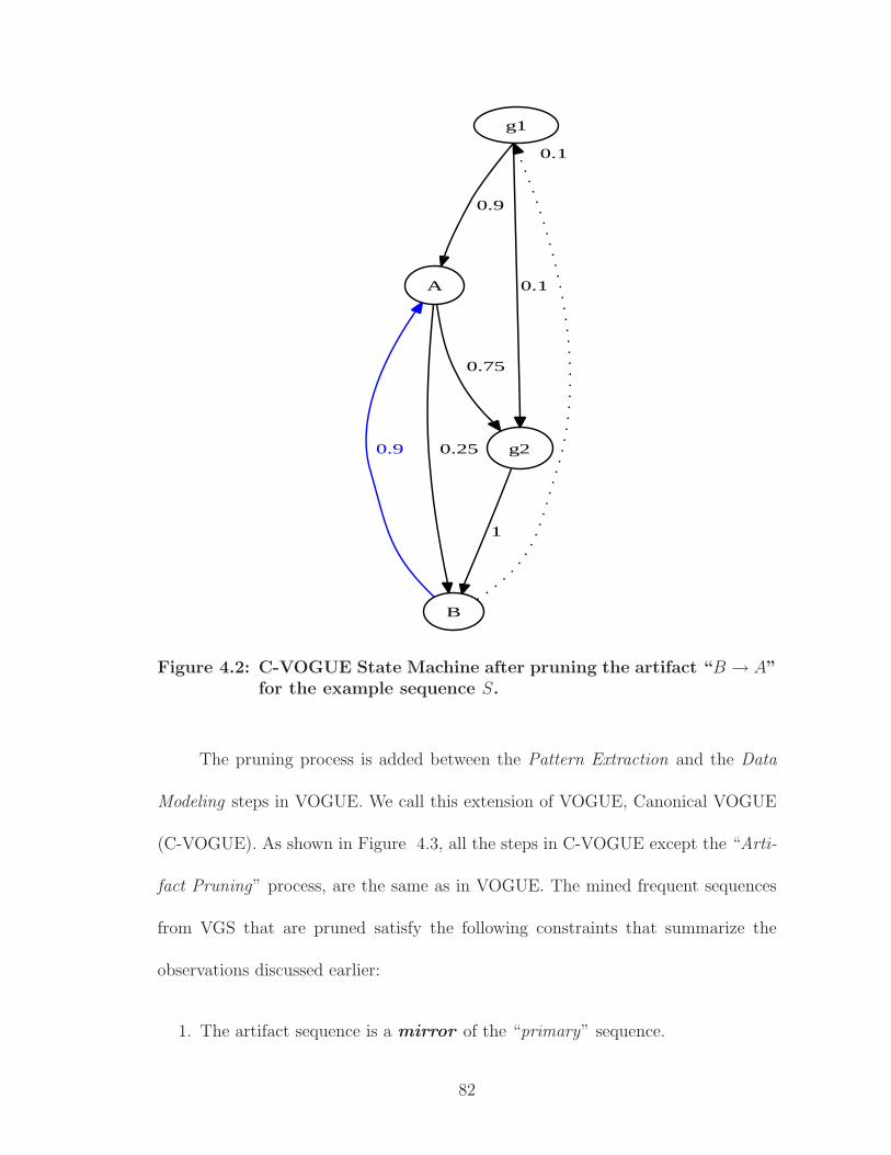
g1
A
0.9
g2
0.1
B
0.25
0.75
0.1
0.9
1
Figure 4.2: C-VOGUE State Machine after pruning the artifact “B → A”for the example sequence S.
The pruning process is added between the Pattern Extraction and the Data
Modeling steps in VOGUE. We call this extension of VOGUE, Canonical VOGUE
(C-VOGUE). As shown in Figure 4.3, all the steps in C-VOGUE except the “Arti-
fact Pruning” process, are the same as in VOGUE. The mined frequent sequences
from VGS that are pruned satisfy the following constraints that summarize the
observations discussed earlier:
1. The artifact sequence is a mirror of the “primary” sequence.
82
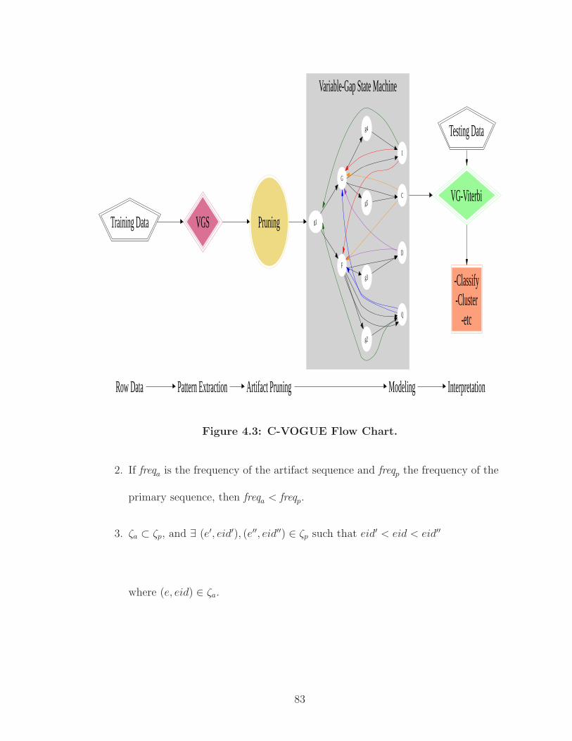
Variable-Gap State Machine
Row Data Pattern Extraction Artifact Pruning Modeling Interpretation
VG-Viterbi
-Classify-Cluster
-etc
Testing Data
Training Data VGS Pruning g1
F
G
Q
D
g2
g3
I
C
g4
g5
Figure 4.3: C-VOGUE Flow Chart.
2. If freqa is the frequency of the artifact sequence and freqp the frequency of the
primary sequence, then freqa < freqp.
3. ζa ⊂ ζp, and ∃ (e′, eid′), (e′′, eid′′) ∈ ζp such that eid′ < eid < eid′′
where (e, eid) ∈ ζa.
83
4.2 K-VOGUE: VOGUE Augmented with Domain Specific
Knowledge
In some domains such as in biological sequence analysis [25, 27], the pat-
terns that are supposed to be frequent do not have an exact match in all the se-
quences that belong to the same family or class, but instead we need to allow inex-
act matches among some elements. These elements, however, share some common
characteristics and thus called “similar”. In fact, in proteins, the motifs (patterns
or frequent subsequences) that characterize a family or class of proteins is a pat-
tern that is found in all the sequences where some elements could be different. In
this case the pattern or motif looks more like a grammar. For example, given the
motif P ={G[IV T ][LV AC][LV AC][IV T ]D[DE][FL][DNST ]}, the subsequences:
(GICCIDEFD), (GV CLIDEFD), (GV CLIDEFD), (GV V CIDEFD), and (GV V CIDEFD)
can interchange. [IV T ] means that either I, V , or T could be found. The elements
that are grouped together are in general amino acids that have similar structure.
For example, I and V belong to the same subgroup, that is non-polar and hy-
drophobic amino acids group as shown in Figure 4.4, [59].
Regular methods that look for exact matches in subsequences to declare them
frequent will miss a pattern such as the motif P . Therefore, there is a need for
methods that allow for substitutions among similar elements to capture such pat-
terns/motifs. In bioinformatics, substitution matrices, [7, 28], have been used to
estimate the rate at which each possible element in a sequence changes to another
element over time. Substitution matrices are used in amino acid sequence alignment,
84
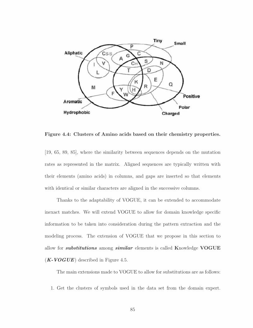
Figure 4.4: Clusters of Amino acids based on their chemistry properties.
[19, 65, 89, 85], where the similarity between sequences depends on the mutation
rates as represented in the matrix. Aligned sequences are typically written with
their elements (amino acids) in columns, and gaps are inserted so that elements
with identical or similar characters are aligned in the successive columns.
Thanks to the adaptability of VOGUE, it can be extended to accommodate
inexact matches. We will extend VOGUE to allow for domain knowledge specific
information to be taken into consideration during the pattern extraction and the
modeling process. The extension of VOGUE that we propose in this section to
allow for substitutions among similar elements is called Knowledge VOGUE
(K-VOGUE) described in Figure 4.5.
The main extensions made to VOGUE to allow for substitutions are as follows:
1. Get the clusters of symbols used in the data set from the domain expert.
85
Otherwise, cluster the alphabet symbols into clusters Ci based on similarity
depending on the problem domain at hand using the domain knowledge. The
clustering method we propose is described in some more detail in Section 4.3.
2. Replace each element in the data set that belongs to a cluster Ci, by a symbol
ci that represents the cluster Ci. Therefore, the symbol alphabet now becomes
the set∑′ = {ci, i{1, · · · , L}}, where L is the number of clusters Ci. Therefore
the alphabet symbol is no longer the original symbol set∑
but the new symbol
alphabet∑′.
3. Mine the data set for frequent subsequences using VGS according to a user
defined min sup, maxgap and length k.
4. Modeling the mined patterns could be done in two ways:
(a) Build the variable-order gap state machine directly from the mined pat-
terns by VGS with the symbol states Qf and Qs still emitting only one
symbol with probability 1. In this case, the symbols are the representa-
tives ci of the clusters Ci, i ∈ {1, · · · , L} and not the original alphabet
symbol∑
. For example, let’s consider the cluster that has been identi-
fied as C1 = {I, V, T} and the representative symbol is c1 = I. In this
case, the symbol states Qf and Qs, in the variable-Order state machine,
produce only one symbol. That symbol is the representative symbol of
one of the clusters Ci. In our example, one of the sates in Qf emits I the
representative of the cluster C1. Therefore, for the Interpretation step
86
we need to replace the elements in the testing data set with the cluster
representatives ci, i ∈ {1, · · · , L} then use VG-Viterbi with the modified
testing data set.
(b) Build a variable-order gap state machine that allows several emissions
from the symbol states Qf and Qs. In order to build the variable-order
state machine, we use the frequent sequences mined by VGS from the
modified data set,but the only difference is that the state symbols Qf and
Qs can emit any symbol, vm, from the corresponding cluster Ci, rather
than emitting only one symbol from the modified symbol alphabet∑′.
In our running example, a state in Qf can emit any symbol vm from
C1 = {I, V, T}. The emission probability in this case, is computed as
follows:
b(qi, vm) =freqi(vm)
∑
vm∈Cifreqi(vm)
(4.1)
Note that only the symbols belonging to the cluster Ci will be emitted.
The symbols from the alphabet∑
that do not belong to the cluster
Ci will be emitted with probability 0. For example, let’s assume that
the frequency of I, V , and T , were 6, 4, and 1 respectively. Then the
emission probability from state q1 for I is b(q1,I) = 66+4+1
= 611
= 0.54,
for V is b(q1, V ) = 0.36, and for T is b(q1, T ) = 0.09. On the other
hand, for any symbol vm ∈∑
\C1 its corresponding emission probability
is b(q1, vm) = 0. In this case, the VG-Viterbi will be used directly on the
original testing data set with no replacement.
87
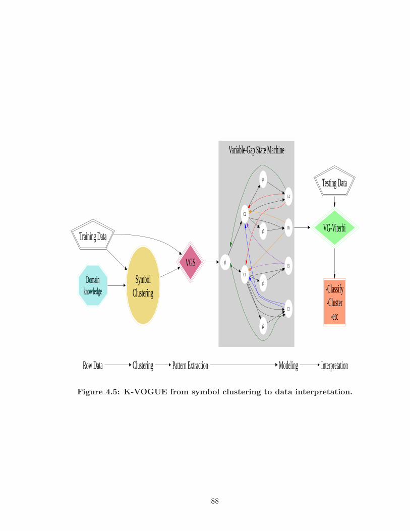
Variable-Gap State Machine
Row Data Clustering Pattern Extraction Modeling Interpretation
VG-Viterbi
-Classify-Cluster
-etc
Testing Data
Training Data
VGS
SymbolClustering
Domainknowledge
g1
C1
C2
C3
C5
g2
g3
C4
C6
g4
g5
Figure 4.5: K-VOGUE from symbol clustering to data interpretation.
88
4.3 Symbol clustering
This section describes the clustering method that we use for clustering the
symbols that will be used in K-VOGUE. Sometimes the clusters of the symbols are
available from the expert in the domain at hand and sometimes they are not. In the
latter case where the information from the domain expert is not available, we can
use a clustering method to get the cluster from some domain information. K-means
is one of the most popular clustering algorithms in data mining. A major drawback
to K-means is that it cannot separate clusters that are non-linearly separable in
input space. In many real world problems where we need to cluster the symbols,
the clusters could be non-linearly separable like in the case of amino acids as shown
earlier in Figure 4.4. Therefore, K-means, as it is, will not be a good clustering
algorithm. Two recent approaches have emerged for tracking the problem. One is
kernel K-means, where, before clustering, points are mapped to a higher-dimensional
feature space using a nonlinear function, and then kernel k-means partitions the
points by linear separators in the new space. The second approach is spectral
clustering algorithms, which use the eigenvectors of a similarity matrix to partition
points into disjoint clusters, with points in the same cluster having high similarity
and points in different clusters having low similarity. Spectral clustering has many
applications in machine learning, exploratory data analysis, computer vision and
speech processing [95, 100]. Most techniques explicitly or implicitly assume a metric
or a similarity structure over the space of configurations, which is then used by
clustering algorithms. The success of such algorithms depends heavily on the choice
89
of the metric, but this choice is generally not treated as part of the learning problem.
Thus, time-consuming manual feature selection is often a necessary precursor to the
use of spectral methods. Several recent papers have considered ways to alleviate
this burden by incorporating prior knowledge into the metric, either in the setting
of K-means clustering [88, 93] or spectral clustering [95, 100]. Several algorithms
have been proposed in the literature [51, 67, 82], each using the eigenvectors in
slightly different ways. A popular objective function used in spectral clustering is to
minimize the normalized cut [82]. The k-way normalized cut problem is considered
in [96] to partition the data set into k clusters. We will describe in some more
detail the k-way normalized cut spectral clustering since it is the one that we will
be using as clustering technique. If we represent the data set to be clustered as a
graph G = (V , E), where V is the set of vertices representing data points, E is the set
of edges connecting the vertices indicating pair-wise similarity between the points.
The definition of a “good” clustering is that points belonging to the same cluster
should be highly similar while the points belonging to different clusters should be
highly dissimilar. Then represent the similarity graph as a matrix A called edge
similarity matrix, assumed to be nonnegative and symmetric. If n = |E|, then A is
an n×n matrix and Aij is the edge weight between vertex i and j. The eigenvalues
and eigenvectors of the matrix A provide global information about its structure.
Let’s consider v and u as two subsets of V , a link is defined as:
link(u, v) =∑
i∈u,j∈v
A(i, j) (4.2)
90
Then the normalized link-ratio of u and v is:
normallinkratio(u, v) =links(u, v)
links(u,V)(4.3)
The k-way normalized cut problem is to minimize the links in a cluster relative
to the total “weight” of the cluster. For k-way partitioning of the vertices, solving
the following problem is of interest:
min1
k
k∑
j=1
normalinkratio(Vj,V\Vj). (4.4)
This problem was relaxed in [96] by the following spectral relaxation: Let D
be the diagonal matrix where Dii =∑
j Aij. Therefore, the normalized cut criterion
is equivalent to:
max1
ktrace(ZT AZ) (4.5)
where Z = X(XT DX)−1/2, and X is an n × k indicator matrix for the parti-
tions and ZT DZ = Ik.
If we define Z = D1/2Z and relaxing the constraint that X is an indicator
matrix, then the problem becomes a maximization of the trace of ZD−1/2AD−1/2Z,
where the constraints on Z are relaxed such that ZT Z = Ik. This can be solved in
turn by setting the matrix Z to be the top k eigenvectors of the matrix D−1/2AD−1/2.
Therefore the clustering algorithm is described as follows:
1. Pre-processing: Construct the scaled adjacency matrix A′ = D−1/2AD−1/2
91
2. Decomposition:
• Find the eigenvalues and eigenvectors of A′.
• Build embedded space from the eigenvectors corresponding to the k
largest eigenvalues.
3. Grouping: Apply k-means to reduced n × k space to produce k clusters.
4.4 Summary
In this chapter we described two variations of VOGUE, namely, Canonical
VOGUE (C-VOGUE) and Knowledge VOGUE (K-VOGUE). C-VOGUE intends
to decrease even more the state space complexity of VOGUE by pruning frequent
sequences mined by VGS, that are artifacts of other “primary” frequent sequences.
K-VOGUE allows for sequences to form the same frequent pattern even if they do
not have an exact match of elements in all the positions. However, the different
elements have to share “similar” characteristics. This type of patterns are common
in some domains such as in protein classification where certain different elements
of the proteins, known as amino acids, share similar functionality. This is useful in
data sets where the information in the sequences themselves is not sufficient for an
accurate classification but the domain knowledge is also necessary. Furthermore, we
propose to use spectral clustering [95, 100], if the clustering of the symbols in the
training data set is not available.
In the next chapter, we describe the “Interpretation” step of VOGUE.
92
Chapter 5Decoding and
Interpretation
After extracting the patterns and modeling the data, the model is ready to be used
to decode or interpret new observation sequences to answer some questions. For
instance in the domain of biological sequence analysis, there is a need to know
whether or not a protein shares similar properties with a number of other proteins.
This is equivalent to asking if that protein contains the same patterns as the proteins
belonging to the same family that is summarized in the model. Another question,
in the domain of image segmentation, could be finding the “best” segmentation of
scanned images of printed bilingual dictionaries [52] against a built model.
These questions are equivalent to finding the best state sequence in the model.
This problem is referred to in HMMs [75] as the decoding problem. This problem
is difficult to solve since it has several possible ways of solving it. In fact, finding
the best state sequence is equivalent to finding the optimal state sequence that
will decode or interpret the new observation sequence. Therefore, there are several
optimality criteria. One possible solution would be to choose individually the most
likely states qt. Let the probability of being in state si at time t, given the observation
93
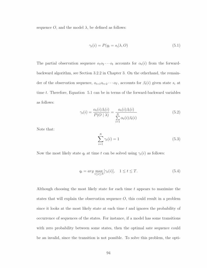
sequence O, and the model λ, be defined as follows:
γt(i) = P (qt = si|λ,O) (5.1)
The partial observation sequence o1o2 · · · ot accounts for αt(i) from the forward-
backward algorithm, see Section 3.2.2 in Chapter 3. On the otherhand, the remain-
der of the observation sequence, ot+1ot+2 · · · oT , accounts for βt(i) given state si at
time t. Therefore, Equation 5.1 can be in terms of the forward-backward variables
as follows:
γt(i) =αt(i)βt(i)
P (O | λ)=
αt(i)βt(i)N∑
i=1
αt(i)βt(i)
(5.2)
Note that:N
∑
i=1
γt(i) = 1 (5.3)
Now the most likely state qt at time t can be solved using γt(i) as follows:
qt = arg max1≤i≤N
[γt(i)], 1 ≤ t ≤ T . (5.4)
Although choosing the most likely state for each time t appears to maximize the
states that will explain the observation sequence O, this could result in a problem
since it looks at the most likely state at each time t and ignores the probability of
occurrence of sequences of the states. For instance, if a model has some transitions
with zero probability between some states, then the optimal sate sequence could
be an invalid, since the transition is not possible. To solve this problem, the opti-
94
mization should be on the state sequence or path. This is equivalent to maximizing
P (Q,O | λ). The most widely used method to solve for this optimization problem
is the Viterbi algorithm [39, 87], a technique based on dynamic programming.
For VOGUE, we can use the same concept to answer the question of inter-
pretation. However, because of VOGUE’s unique structure and needs, we modified
the Viterbi algorithm to handle the notion of duration in the states. This is very
important since VOGUE’s gap states have the notion of duration. This changes the
search for the optimal path to traverse the model’s states as opposed to a regular
HMM. We call this new proposed algorithm as, Variable-Gap Viterbi (VG-Viterbi).
The remainder of this chapter is organized as follows: first we give a description
of the Viterbi algorithm since it is the basis for our VG-Viterbi. Then, we describe
our proposed method, VG-Viterbi.
5.1 Viterbi Algorithm
Finding the best sequence of states q∗ for the observation sequence O =
{o1o2 · · · oT} given the model λ, in the Viterbi algorithm [39, 87], is equivalent
to solving:
q∗ = arg maxq
P (q|λ,O) (5.5)
where q∗ = {q∗1, q∗2, · · · , q∗T}. Now we need to define the highest probability along
a single path, at time t, which accounts for the first observations in O and ends in
95
state si by the quantity:
δt(i) = maxq1q2···qt−1
P (q1q2 · · · qt = i, qt+1 6= i, o1o2 · · · ot|λ) (5.6)
By induction:
δt+1(i) = [maxi
δt(i)aij] · bj(ot+1) (5.7)
To retrieve the best state sequence q∗, the arguments which maximize Equation 5.7
need to be accounted for each t and j. This can be done by using:
ψt(j) = arg max1≤i≤N
[δt−1(i)aij] (5.8)
The procedure for finding the optimal path (sequence of states) that describes the
observation sequence O, [87] is as follows:
1. Initialization:
δ1(i) = πibi(o1), 1 ≤ i ≤ N (5.9)
ψt(i) = 0. (5.10)
2. Recursion:
δt(i) = max1≤i≤N
[δt−1(i)aij]bj(ot), 2 ≤ t ≤ T , 1 ≤ j ≤ N (5.11)
ψt(j) = arg max1≤i≤N
[δt−1(i)aij], 2 ≤ t ≤ T , 1 ≤ j ≤ N (5.12)
96
3. Termination:
p∗ = max1≤i≤N
[δT (i)] (5.13)
q∗ = arg max1≤i≤N
[δT (i)]. (5.14)
4. Path (state sequence) backtracking:
q∗t = ψt+1(q∗t+1), t = T − 1, T − 2, · · · , 1. (5.15)
5.2 VG-Viterbi: Variable Gap Viterbi
Once VOGUE is built to model a data set, and given a new sequence of
observations O = o1o2 · · · oT , there is a need to know whether this sequence belongs
to the same class/family of the training data sequences. In other words, there is
a need to interpret the new sequence based on the built model λ. This problem is
equivalent to finding the best sequence of states from the model λ and gap state
duration length that will describe the new sequence in an optimal and meaningful
way. That is finding a sequence of states q∗ = {q∗1, q∗2, · · · , q∗T} from the model λ
such that:
q∗ = arg maxq
P (q|λ,O) (5.16)
This is equivalent to finding the most probable path to be traversed in λ that
would produce O. The algorithm that is mostly used to solve this problem is the
Viterbi algorithm [39, 87]. Due to the unique structure of VOGUE, where gap
states have a notion of duration, we adjusted the Viterbi algorithm accordingly. We
97
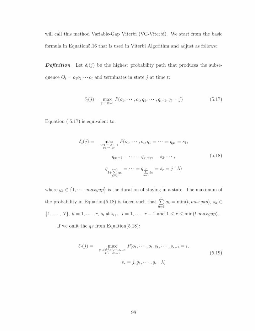
will call this method Variable-Gap Viterbi (VG-Viterbi). We start from the basic
formula in Equation5.16 that is used in Viterbi Algorithm and adjust as follows:
Definition Let δt(j) be the highest probability path that produces the subse-
quence Ot = o1o2 · · · ot and terminates in state j at time t:
δt(j) = maxq1···qt−1
P(o1, · · · , ot, q1, · · · , qt−1, qt = j) (5.17)
Equation ( 5.17) is equivalent to:
δt(j) = maxr,s1,··· ,sr−1
g1,··· ,gr
P(o1, · · · , ot, q1 = · · · = qg1 = s1,
qg1+1 = · · · = qg1+g2 = s2, · · · ,
q1+
r−1P
h=1gh
= · · · = q rP
h=1
gh
= sr = j | λ)
(5.18)
where gh ∈ {1, · · · ,maxgap} is the duration of staying in a state. The maximum of
the probability in Equation(5.18) is taken such thatr
∑
h=1
gh = min(t,maxgap), sh ∈
{1, · · · , N}, h = 1, · · · , r, sl 6= sl+1, l = 1, · · · , r − 1 and 1 ≤ r ≤ min(t,maxgap).
If we omit the qs from Equation(5.18):
δt(j) = maxgr,i6=j,s1,··· ,sr−2
g1,··· ,gr−1
P(o1, · · · , ot, s1, · · · , sr−1 = i,
sr = j, g1, · · · , gr | λ)
(5.19)
98
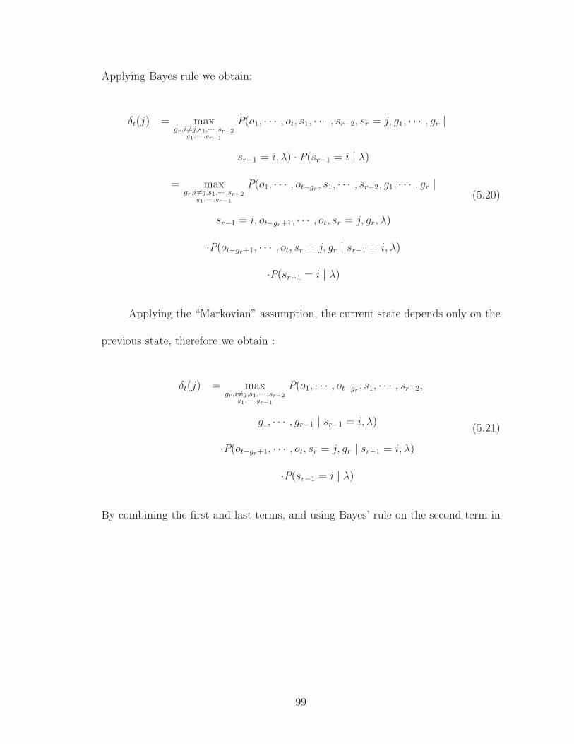
Applying Bayes rule we obtain:
δt(j) = maxgr,i6=j,s1,··· ,sr−2
g1,··· ,gr−1
P(o1, · · · , ot, s1, · · · , sr−2, sr = j, g1, · · · , gr |
sr−1 = i, λ) · P(sr−1 = i | λ)
= maxgr,i6=j,s1,··· ,sr−2
g1,··· ,gr−1
P(o1, · · · , ot−gr, s1, · · · , sr−2, g1, · · · , gr |
sr−1 = i, ot−gr+1, · · · , ot, sr = j, gr, λ)
·P(ot−gr+1, · · · , ot, sr = j, gr | sr−1 = i, λ)
·P(sr−1 = i | λ)
(5.20)
Applying the “Markovian” assumption, the current state depends only on the
previous state, therefore we obtain :
δt(j) = maxgr,i6=j,s1,··· ,sr−2
g1,··· ,gr−1
P(o1, · · · , ot−gr, s1, · · · , sr−2,
g1, · · · , gr−1 | sr−1 = i, λ)
·P(ot−gr+1, · · · , ot, sr = j, gr | sr−1 = i, λ)
·P(sr−1 = i | λ)
(5.21)
By combining the first and last terms, and using Bayes’ rule on the second term in
99
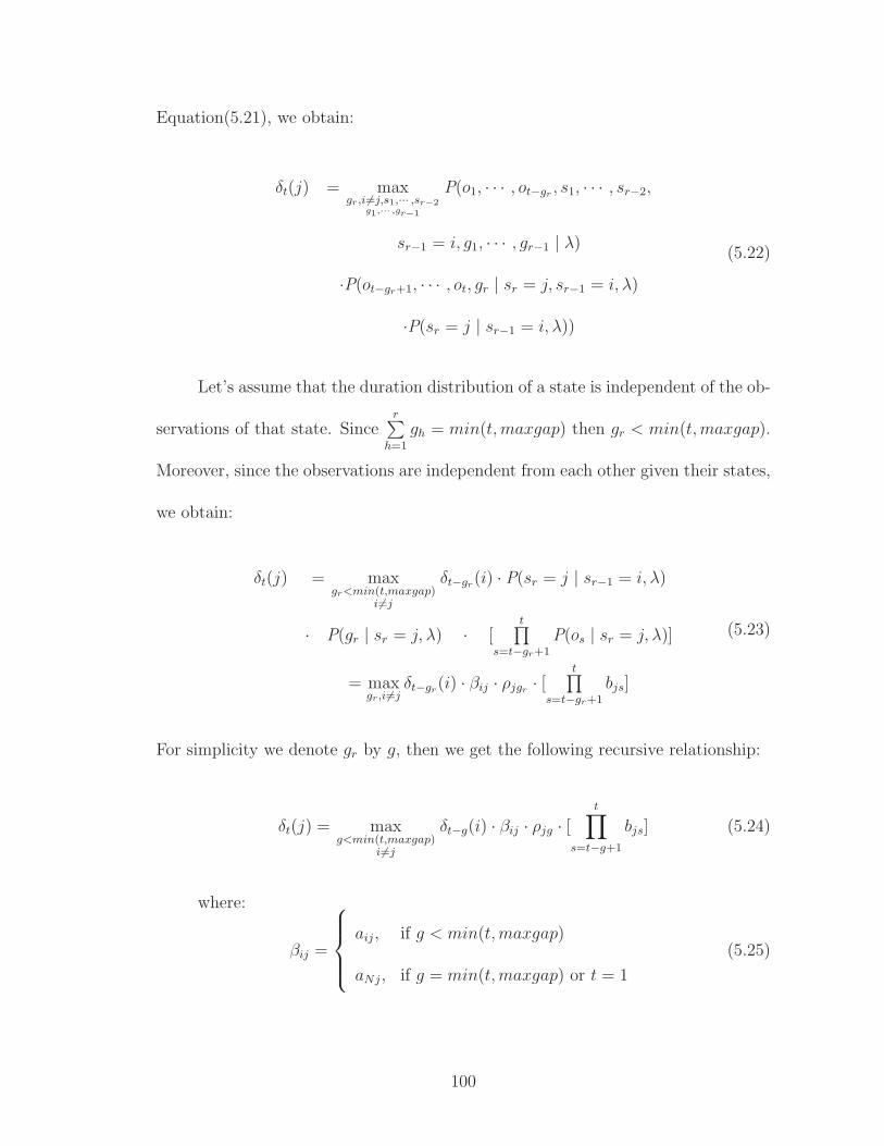
Equation(5.21), we obtain:
δt(j) = maxgr,i6=j,s1,··· ,sr−2
g1,··· ,gr−1
P(o1, · · · , ot−gr, s1, · · · , sr−2,
sr−1 = i, g1, · · · , gr−1 | λ)
·P(ot−gr+1, · · · , ot, gr | sr = j, sr−1 = i, λ)
·P(sr = j | sr−1 = i, λ))
(5.22)
Let’s assume that the duration distribution of a state is independent of the ob-
servations of that state. Sincer
∑
h=1
gh = min(t,maxgap) then gr < min(t,maxgap).
Moreover, since the observations are independent from each other given their states,
we obtain:
δt(j) = maxgr<min(t,maxgap)
i6=j
δt−gr(i) · P(sr = j | sr−1 = i, λ)
· P(gr | sr = j, λ) · [t
∏
s=t−gr+1
P(os | sr = j, λ)]
= maxgr,i6=j
δt−gr(i) · βij · ρjgr
· [t
∏
s=t−gr+1
bjs]
(5.23)
For simplicity we denote gr by g, then we get the following recursive relationship:
δt(j) = maxg<min(t,maxgap)
i6=j
δt−g(i) · βij · ρjg · [t
∏
s=t−g+1
bjs] (5.24)
where:
βij =
aij, if g < min(t,maxgap)
aNj, if g = min(t,maxgap) or t = 1
(5.25)
100
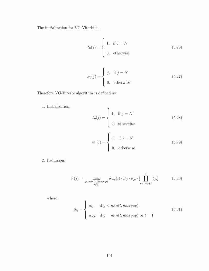
The initialization for VG-Viterbi is:
δ0(j) =
1, if j = N
0, otherwise
(5.26)
ψ0(j) =
j, if j = N
0, otherwise
(5.27)
Therefore VG-Viterbi algorithm is defined as:
1. Initialization:
δ0(j) =
1, if j = N
0, otherwise
(5.28)
ψ0(j) =
j, if j = N
0, otherwise
(5.29)
2. Recursion:
δt(j) = maxg<min(t,maxgap)
i6=j
δt−g(i) · βij · ρjg · [t
∏
s=t−g+1
bjs] (5.30)
where:
βij =
aij, if g < min(t,maxgap)
aNj, if g = min(t,maxgap) or t = 1
(5.31)
101
5.3 VG-Viterbi: optimization
Since VG-Viterbi is based on the Viterbi algorithm [87], it inherits its ad-
vantages and drawbacks. One of the drawbacks of the Viterbi algorithms is that it
exhaustively searches the state space of the HMM to find the best (optimal) path
of state sequences to describe the observation sequence O. If N is the number of
states of the model λ, and T is the length of O, then the Viterbi algorithm’s time
complexity is O(N2 × T ) [39, 87]. This is obviously expensive when the number of
states N is large and the observation sequence is very long. In fact in some areas like
in biological sequence analysis [27], where the length of a sequence varies between
500 and 1000 elements, and when the HMM is about 900 states the estimated time
complexity of the Viterbi algorithm is on the order of 8 × 10⁸. The time complex-
ity of the VG-Viterbi algorithm is comparable to that of the Viterbi algorithm. In
fact, let N be the number of states in VOGUE, and the length of the observation
sequence O be T . In the case of an exhaustive search of the model λ, for every
element Ot in O (0 ≤ t ≤ T ), we need to check for the highest probability of Ot to
be emitted by a state qi where 1 ≤ i ≤ N . This is done by taking into consideration
the state qj that has the highest probability of emitting Ot−1. Moreover, some of
the states are “gap” states, and they have a notion of duration up to maxgap times.
Hence, we need to explore the number of O’s elements that will be emitted from the
same “gap” state, i.e., “staying” in the same state for up to maxgap. Therefore, the
estimated time is O(N ×N ×maxgap×T ). In order to reduce the time complexity
we need to reduce either N , maxgap or T . Since we cannot reduce T , which is the
102
length of the observation sequence, we have to explore reducing either maxgap or
N .
VOGUE is not a fully connected graph, since all the states are not connected
to all the states. In fact, the only possible transitions, whose probability is nonzero
are the following transitions:
• Transitions from the Universal Gap state to the first state symbols qj ∈ Qf
and to the intermediate gap states qj ∈ Qi. Therefore the number of allowed
transitions (nonzero transitions) from the Universal Gap state is | Qf | +
| Qi |.
• Transitions from the first state symbols qi ∈ Qf to a second state symbol
qj ∈ Qs (modeling a gap of g = 0) or to an intermediate gap state qj ∈ Qi.
Therefore the number of allowed transitions (nonzero transitions) from the
first state symbols is | Qs | + | Qi |.
• Transitions from the intermediate gap state qi ∈ Qi to only a second state sym-
bol qj ∈ Qs. Therefore the number of allowed transitions (nonzero transitions)
from the intermediate gap state is | Qs |.
• Transitions from the second symbol state qi ∈ Qs to a first state symbol qj ∈ Qf
(modeling a gap of g = 0) or to the Universal Gap state qj ∈ Qu. Therefore
the number of allowed transitions (nonzero transitions) from the intermediate
gap state is | Qf | + | Qu |.
Therefore the transition matrix A is a sparse matrix as shown in Equation
103
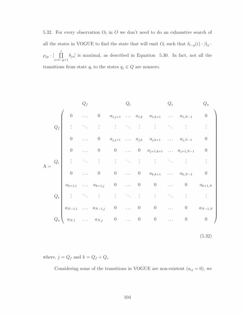
5.32. For every observation Ot in O we don’t need to do an exhaustive search of
all the states in VOGUE to find the state that will emit Ot such that δt−g(i) · βij ·
ρjg · [t
∏
s=t−g+1
bjs] is maximal, as described in Equation 5.30. In fact, not all the
transitions from state qt to the states qj ∈ Q are nonzero.
A =
Qf Qi Qs Qu
0 . . . 0 a1,j+1 . . . a1,k a1,k+1 . . . a1,N−1 0
Qf...
. . ....
.... . .
......
. . ....
...
0 . . . 0 aj,j+1 . . . aj,k aj,k+1 . . . aj,N−1 0
0 . . . 0 0 . . . 0 aj+1,k+1 . . . aj+1,N−1 0
Qi...
. . ....
.... . .
......
. . ....
...
0 . . . 0 0 . . . 0 ak,k+1 . . . ak,N−1 0
ak+1,1 . . . ak+1,j 0 . . . 0 0 . . . 0 ak+1,N
Qs...
. . ....
.... . .
......
. . ....
...
aN−1,1 . . . aN−1,j 0 . . . 0 0 . . . 0 aN−1,N
Qu aN,1 . . . aN,j 0 . . . 0 0 . . . 0 0
(5.32)
where, j = Qf and k = Qf + Qi.
Considering some of the transitions in VOGUE are non-existent (aij = 0), we
104
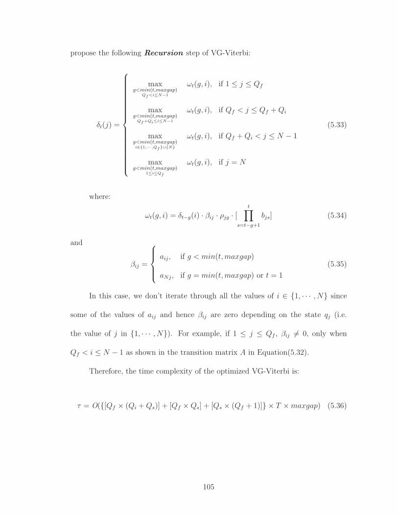
propose the following Recursion step of VG-Viterbi:
δt(j) =
maxg<min(t,maxgap)
Qf <i≤N−1
ωt(g, i), if 1 ≤ j ≤ Qf
maxg<min(t,maxgap)
Qf +Qi≤i≤N−1
ωt(g, i), if Qf < j ≤ Qf + Qi
maxg<min(t,maxgap)i∈{1,··· ,Qf }∪{N}
ωt(g, i), if Qf + Qi < j ≤ N − 1
maxg<min(t,maxgap)
1≤i≤Qf
ωt(g, i), if j = N
(5.33)
where:
ωt(g, i) = δt−g(i) · βij · ρjg · [t
∏
s=t−g+1
bjs] (5.34)
and
βij =
aij, if g < min(t,maxgap)
aNj, if g = min(t,maxgap) or t = 1
(5.35)
In this case, we don’t iterate through all the values of i ∈ {1, · · · , N} since
some of the values of aij and hence βij are zero depending on the state qj (i.e.
the value of j in {1, · · · , N}). For example, if 1 ≤ j ≤ Qf , βij 6= 0, only when
Qf < i ≤ N − 1 as shown in the transition matrix A in Equation(5.32).
Therefore, the time complexity of the optimized VG-Viterbi is:
τ = O({[Qf × (Qi + Qs)] + [Qf × Qs] + [Qs × (Qf + 1)]} × T × maxgap) (5.36)
105
which becomes:
τ = O({[Qi × (Qf + Qs)] + 2Qs × [Qf + 1]} × T × maxgap)
= O({Qi × (Qf + Qs)} × T × maxgap) + 2O({Qs × (Qf + 1)} × T × maxgap)
(5.37)
Qf and Qs never exceed M the number of observations in VOGUE since they
are the number of “distinct” first and second symbols in the mined sequences by
VGS, respectively. In fact there could be at most M different symbols identified
by VGS. Since M is always a fixed number as opposed to the number of sequences
retained by VGS, reflected by Qi, when N is large Qi large. Therefore, O(Qi×(Qf +
Qs)×T ×maxgap) ≤ O(Qi×2M ×T ×maxgap), and O(Qi×2M ×T ×maxgap) ≃
2MO(Qi × T × maxgap) ≃ O(Qi × T × maxgap). Likewise, O(Qs × (Qf + 1) ×
T ×maxgap) ≤ O(M(M + 1) × T ×maxgap) and O(M(M + 1) × T ×maxgap) ≃
O(T × maxgap).
Therefore, τ ¹ O((Qi + 1) × T × maxgap) ≪ O(N2 × T × maxgap), since
Qi < N .
5.4 Summary
In this chapter, we described the “interpretation” step of VOGUE. In fact,
after extracting and modeling the data, the model is ready to be used to interpret
new observation sequences and identify if the observation sequence belongs to the
“same” class or family as the training data set. This question is equivalent to find-
ing the “best”, or optimal, state sequence in the model that best “interprets” the
106

new observed sequence. The most widely used algorithm to solve this optimization
problem is the Viterbi algorithm [39, 87], a technique based on dynamic program-
ming. Because of VOGUE’s unique structure, we modified the Viterbi algorithm.
In fact, the Viterbi algorithm does not account for the notion of duration in the
states that is present in the intermediate gap states in VOGUE. We call this new
proposed algorithm as Variable-Gap Viterbi.
In the next chapter, we show some experimental results on real data sets from
the protein families of VOGUE as opposed to some state-of-the art methods in
protein classification.
107
Chapter 6Experimental Results and
Analysis
Several real world applications, such as in bioinformatics, web accesses, finance, and
text mining, encompass sequential and temporal data with long range dependencies.
The fact that VOGUE has been designed to capture and model such long range
dependency patterns, makes it a very good tool to model some of those applications.
In [2], we developed a toolkit to facilitate the sharing and long term use of different
types of geological data sets across disciplines. Geoscientists are confronted with an
enormous quantity of diverse data types. These data sets include published data,
geological and topological maps, satellite imagery, structural, seismic, geophysical,
petrologic and geochronologic data. The time when the data are added or accessed
by users is recorded. While each piece of data originates at a specific user, each user
is allowed to add new annotations to the data as they wish. Finding where the data
is and what type of data a user should access next is a challenging problem. We use
VOGUE as the core of this toolkit to model user access patterns of the data in the
database. Moreover, it allows a new user to visualize the most common patterns of
use or the latest common patterns of use based on the data set used to construct the
108
VOGUE state machine. When a user accesses and adds new data to the database,
he/she starts a new project. A specific project may have multiple patterns of use
at the same granularity corresponding to different research activities or problems
being investigated. We built different VOGUE state machines to accommodate the
multiple views corresponding to different interpretations of the data.
In this chapter, though, we describe several experiments that we conducted to
compare the performance of VOGUE, C-VOGUE and K-VOGUE to those of two
popular techniques in the domain of biological sequence analysis: HMMER and all-
kth-order HMM. We used two data sets, a real data set from the PROSITE database,
a sequential data base of families of proteins, and the SCOP data set, a manually
derived comprehensive hierarchical classification of known proteins structures that
has secondary structure knowledge embedded in the data set.
6.1 Protein modeling and clustering using VOGUE
The completion of the whole genome sequencing of various organisms facil-
itates the detection of many kinds of interesting patterns in DNA and protein
sequences. It is known that the genomes of most plants and animals contain large
quantities of repetitive DNA fragments or, in the case of proteins, Amino Acid frag-
ments. For instance, it is estimated that one third of the human genome is composed
of families of repeating sequences [32, 33, 102]. The amino acids are thus far from
being pieces of random sequences, and a substantial amount of currently unknown
information can be extracted from the sequences in the form of patterns. The abun-
dance and variety of periodic patterns in genome sequences drove a lot of studies on
109
genome sequence analysis and mining. In fact, periodic patterns of different lengths
and types are found at both geneomic and proteomic levels. The short three base
pair (bp) periodicity in protein coding DNA [38], and the medium-length repetitive
motifs found in some proteins [21], to the mosaic of very long DNA segments in the
genome of warm-blooded vertebrates [16], are some of these patterns. It is very
important to identify some of these patterns due to their biological significance. For
instance, some repeats have been shown to affect bacterial virulence to human be-
ing [86]. On the other hand, the excessive expansions of some Variable Number of
Tandem Repeats (V NTRs) are the suspected cause of some nervous system diseases
[76]. Therefore, there is a growing need for efficient algorithms to extract periodic
patterns from long sequences.
In recent years, a large amount of work in biological sequence analysis has
focused on methods for finding homologous proteins [27]. Given a database of
protein sequences, the goal is to build a statistical model so that we can determine
whether a query protein belongs to a given family or not. HMMER [30], a profile
HMM, is one of the state-of-the-art approaches to this problem that depends heavily
on a good multiple sequence alignment. It models gaps, provided that they exist in
the alignment of all the training sequences. However, if a family of sequences has
several overlapping motifs, which may occur in different sequences, these sequences
will not be aligned correctly, and HMMER will not perform well. Here, we analyze
the performance of VOGUE compared to HMMER and higher-order HMMs with
various orders k ∈ [1, 10].
Computationally, protein sequences are treated as long strings of characters
110
with a finite alphabet of 20 amino acids. Namely, A, C, D, E, F , G, H, I, K, L,
M , N , P , Q, R, S, T , V , W , and Y . There are many patterns depending on the
issues considered, for example the number of periods of the patterns, the maximality
of the patterns, whether errors (insertions, deletions and substitutions) are allowed
and palindromic reverses. In [55], the authors provide a survey on studies to extract
patterns taking into consideration one of the issues mentioned earlier.
In this work, we are particularly interested in extracting patterns that identify
a family of proteins. The first method focuses on extracting those patterns from
the sequences formed of the 20 amino acids and not allowing any substitutions be-
tween them. The second method, extracts patterns while allowing for substitutions
between amino acids that have similar structure and functionality (Hydrophobicity,
Charge, Polarity, etc).
We apply VOGUE, C-VOGUE, and K-VOGUE to a real world problem,
namely, finding homologous proteins. Given a database of protein sequences, the
goal is to build a statistical model so that we can determine whether a query protein
belongs to a given family or not. Statistical models for proteins, such as profiles,
position-specific scoring matrices, and hidden Markov models [27] have been devel-
oped to find homologs. However, in most biological sequences interesting patterns
are periodic with gap requirements. Therefore a method like VOGUE that specifi-
cally takes these kind of patterns into consideration can be very effective. We show
experimentally that VOGUE’s modeling power is superior to higher-order HMMs
while reducing the latter’s state-space complexity, and improving their prediction.
VOGUE also outperforms HMMER [30], a HMM model especially designed for pro-
111

tein sequences that takes into consideration insertions, deletions and substitutions
between “omosimilar” amino acids. We will give a an overview of HMMER in
Section 6.1.1. Then, we will describe the scoring and evaluation measure we use
for evaluating the performance of the methods used. Afterwards, we describe the
data sets that we use for our experimentation. Finally, we provide the performance
results of VOGUE, C-VOGUE and K-VOGUE vs HMMER and higher-order HMM.
6.1.1 HMMER
HMMER [30] is a HMM model especially designed for protein sequences that
takes into consideration insertions, deletions and substitutions between “omosimilar”
amino acids. It is called a “Profile” HMM, a well suited HMM for multiple align-
ments of sequences. We will to first describe what a multiple alignment is, and then
describe a “Profile” HMM.
Multiple Alignment : the problem of multiple alignment is described as follows:
Given a set of sequences, produce a multiple alignment which corresponds as
well as possible, to the biological relationships between the corresponding bio-
molecules [27]. Two amino acids should be aligned (on top of each other) in
the following conditions:
• if they are homologous (evolved from the same residue in a common
ancestor).
• if they are structurally equivalent.
To identify whether an alignment is good, a fitness function is used where the
112
biological relationships are taken into considerations. For example, assuming
the following three sequences:
I N D U S T R Y
I N T E R E S T I N G
I M P O R T A N T
One alignment could be :
I N − D U − S T R Y −
I N T E R E S T I N G
I M − P O R − T A N T
But the following is not a good alignment based on the biological characteris-
tics of the amino acids:
I N − D U − − S T R Y −
I N T E R E − S T I N G
I M − P O R − − T A N T
For a more detailed description of the multiple alignment process and the
different available methods refer to [69].
Profile HMM : One of the general features of protein family multiple alignment is
that “gaps” tend to line up with each other, leaving solid blocks of either exact
matches or allowed substitutions between the amino acids. These positions are
considered to be the “ungapped” states of the HMM. The emission probability
is based on a position specific score matrix (PSSM). More details can be found
113
Begin
I0
M1
D1
I1
Mj
Dj
Ij
Mn
D3
I3
end
Figure 6.1: The transition structure of a profile HMM.
in [27]. Thus, the HMM is built with a repetitive structure of states but
different probabilities in each one in a left-to-right manner. The PSSM is a
HMM with a series of identical states, called “match states” (Mj), separated
by transitions of probability 1. Although PSSM captures some conservation
information, it is does not represent all the information in a multiple alignment
of a protein family. Therefore, “Insertion” states (Ij) are introduced in the
HMM, where each of the Ij states is used to match insertion after the element
emitted by the matching state Mj. “Deletion” states (Dj) are also added to
act as silent states that do not emit any symbol. Therefore, it is possible to
use them to “jump” from any “match” state to another one without emitting
any symbol in between. Figure 6.1 describes a Profile HMM [27].
HMMER is a software that is based on building profile HMMs to model pro-
tein families. Figure 6.2 provides an overview of HMMER. The programs used in
HMMER are as follow:
114

Building a model the part of HMMER software to build a model are:
• hmmbuild: Form multiple sequence alignment.
Using a model • hmmalign: Align sequences to an existing model (outputs a
multiple alignment).
• hmmconvert: Convert a model into different formats.
• hmmcalibrate: Takes an HMM and empirically determines parameters
that are used to make searches more sensitive, by calculating more accu-
rate expectation value scores (E-values).
• hmmemit: Emit sequences probabilistically from profile HMM.
• hmmsearch: Search a sequence database for matches to an HMM.
HMMs Databases the part of HMMER software to handle either a sequence or
HMM database are:
• hmmfetch: Get a single model from an HMM database.
• hmmindex: Index an HMM database.
• hmmpfam: Search an HMM database for matches to a query sequence.
Other programs Other programs that can be used are:
• alistat: Show some simple statistics about a sequence alignment file.
• seqstat: Show some simple statistics about a sequence file.
• getseq: Retrieve a subsequence from a sequence file.
• sreformat: Reformat a sequence or alignment file into a different format.
115
Domains matches?
Multiple alignment alistat
HMM
hmmbuild
hmmsearch
hmmalign
hmmconvert hmmcalibrate Sequences
hmmemit
hmmpfam
hmmalign
seqstat
Sequences database
hmmsearch
getseq
HMM database
hmmpfam
hmmfetch
hmmindex
Figure 6.2: HMMER Flow Chart.
6.1.2 Evaluation and Scoring
We built three models for each family, namely VOGUE, HMMER, and k-th
order HMMs, using the training set of that family. We score the test sequences
against the model for each of the nine families, and after sorting the scores in
decreasing order, we use a threshold on the scores to assign a sequence to a given
family.
For evaluation of the classifiers, we use Receiver Operating Characteristic
(ROC) curves [34], that represent the relationship between the false positive rate
and true positive rate across the full spectrum of threshold values. Further, we plot
116
the Area Under the Curve (AUC), to evaluate the goodness of the classifiers. The
AUC is calculated using the following equation [34]:
AUC =1
pn
p∑
i=1
n∑
j=1
ϕ(Ri, Rj). (6.1)
Here Ntest = n + p is the number of testing sequences, p is the number of sequences
from a given class and n is the number of sequences that don’t belong to the class.
These sequences are ranked based on their score from 1 to Ntest, assigning 1 to the
testing sequence with the highest score and Ntest to the one with the lowest score.
Ri, i = 1 · · · p represent the rankings of the p sequences and Rj, j = 1 · · ·n represent
the rankings of the n sequences and ϕ(Ri, Rj) is defined as:
ϕ(Ri, Rj) =
1 if Ri < Rj
0 otherwise
(6.2)
Note that AUC for each class is calculated separately, by treating each class as p,
and the remaining as n.
We score the testing sequences by computing the log-odds score, (i.e., the ratio
of the probability of the sequence using a given model, and the probability of the
sequence using a Null model, given as follows:
Log-Odds(seq) = log2
(
P (seq|Model)
P (seq|Null)
)
. (6.3)
P (seq/Model) is computed using the Viterbi algorithm that computes the
117
most probable path through the model) as Viterbi is the default method used for
scoring in HMMER. The Null model is a simple one state HMM that emits the
observations (the amino acids) with equal probability (1/|Σ|). Since we have 20
amino acids the emission probability for each symbol is 1/20. The log-odds ratio
measures whether the sequence is a better match to the given model (if the score
is positive) or to the null hypothesis (if the score is negative). Thus, the higher the
score the better the model.
6.1.3 Datasets
We used in our experiments two different data sets: a set of 9 families down-
loaded from the PROSITE (http://www.expasy.org/prosite) database of protein
family and domains, and SCOP [20] data set, a manually derived comprehensive
hierarchical classification of known protein structures, that are organized according
to their evolutionary and structural relationships.
The PROSITE families that we used are PDOC00662, PDOC00670, PDOC00561,
PDOC00064, PDOC00154, PDOC00224, PDOC00271, PDOC00397, PDOC00443.
We will refer to these families as F1, F2, · · · , F9, respectively. The number
of sequences in each family is, respectively: N1 = 45, N2 = 225, N3 = 85,
N4 = 56, N5 = 119, N6 = 99, N7 = 150, N8 = 21, N9 = 29. The fam-
ilies consists of sequences of lengths ranging from 597 to 1043 characters,
taken from the alphabet of the 20 amino acids: Σ = {A, C, D, E, F, G,
H, I, K, L, M, N, P, Q, R, S, T, V, W, Y }. Each family is characterized
by a well-defined motif. Family F1, for example, shares the consensus motif
118

[G] − [IV T ] − [LV AC] − [LV AC] − [IV T ] − [D] − [DE] − [FL] − [DNST ],
which has 9 components. Each component can contain any of the symbols
within the square brackets. For example, for the second component, namely
[IV T ], either I, V or T may be present in the sequences.
We treat each PROSITE family as a separate class. We divided the data set of
each family Fi into two subsets: the training data N itrain consists of 90% of the
data, while the testing data N itest contains the remaining 10%. For example,
N1train = 40 and N1
test = 5. There are a total of 103 test sequences across all
families.
The Scop data set is divided into four hierarchical levels: Class, Fold, Superfam-
ily and Family. For SCOP 1.61 (from 2002), the 44327 protein domains were
classified into 701 folds, resulting in an average of 64 domains per fold. The
number of domains per fold varies in SCOP, where some of the folds, such
as TIM barrels, are highly populated, while some of the folds, such as the
HSP40/DnaJ peptide-binding fold that only contain one protein, contain a
few examples. Therefore, the SCOP is an imbalanced data set. This imbal-
anced proportion of examples in each fold contributes to the poor performance
of classical machine learning techniques such as support vector machines and
neural networks [24]. When learning from such data sets, existing machine
learning approaches tend to produce a strong discriminatory classifier or ”high
accuracy” with very low sensitivity or completeness.
We used 10 superfamilies from the SCOP data set (ftp://ftp.rcsb.org/
119
pub/pdb/derived data/pdb seqres.txt) namely, family 49417, 46458, 46626,
46689, 46997, 47095, 47113, 48508, 69118, and 81296. We will refer to them
as SF1, SF2, SF3, SF4, SF4, SF5, SF6, SF7, SF8, SF9 and SF10 respectively.
Each family has 10 sequences. We divided each family data set into 90% (9
sequences for each family)for training and 10% for testing (1 for each family
to a total of 10 sequences).
6.2 Performance of VOGUE vs HMMER vs k-th Order
HMMs on PROSITE data
We built VOGUE state machines with different values of minsup correspond-
ing to 50%, 75% and 100% of the number of instances in the training data, and
maxgap (10, 15, 20, 25, 30) but with the constant k = 2 for the length of the mined
sequences in VGS. We then choose the best set of parameters and fix them for the re-
maining experiments. To model the data using HMMER, we first need to align the
training sequences using CLUSTAL-W (http://www.ebi.ac.uk/clustalw). We
then build a profile HMM using the multiple sequence alignment and compute the
scores for each test sequence using HMMER, which directly reports the log-odds
scores with respect to the Null model mentioned above. We also built several
k-th order HMMs for various values of k using an open-source HMM software
(http://www.cfar.umd.edu/∼kanungo/software). We tried different values for
the number of states ranging from the size of the protein alphabet (20) to roughly
the size of VOGUE (500) and HMMER (900). A k-th order HMM is built by
120
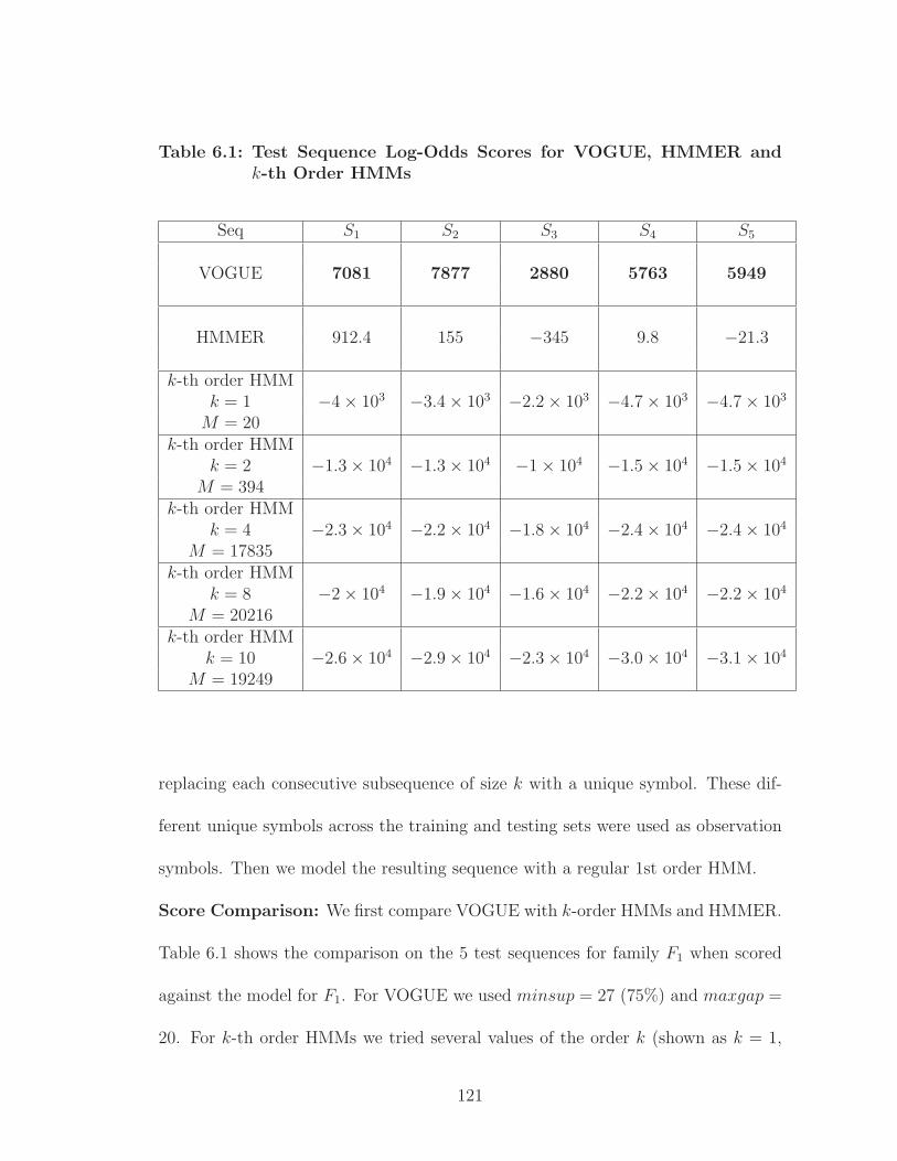
Table 6.1: Test Sequence Log-Odds Scores for VOGUE, HMMER andk-th Order HMMs
Seq S1 S2 S3 S4 S5
VOGUE 7081 7877 2880 5763 5949
HMMER 912.4 155 −345 9.8 −21.3
k-th order HMMk = 1 −4 × 10³ −3.4 × 10³ −2.2 × 10³ −4.7 × 10³ −4.7 × 10³
M = 20k-th order HMM
k = 2 −1.3 × 10⁴ −1.3 × 10⁴ −1 × 10⁴ −1.5 × 10⁴ −1.5 × 10⁴
M = 394k-th order HMM
k = 4 −2.3 × 10⁴ −2.2 × 10⁴ −1.8 × 10⁴ −2.4 × 10⁴ −2.4 × 10⁴
M = 17835k-th order HMM
k = 8 −2 × 10⁴ −1.9 × 10⁴ −1.6 × 10⁴ −2.2 × 10⁴ −2.2 × 10⁴
M = 20216k-th order HMM
k = 10 −2.6 × 10⁴ −2.9 × 10⁴ −2.3 × 10⁴ −3.0 × 10⁴ −3.1 × 10⁴
M = 19249
replacing each consecutive subsequence of size k with a unique symbol. These dif-
ferent unique symbols across the training and testing sets were used as observation
symbols. Then we model the resulting sequence with a regular 1st order HMM.
Score Comparison: We first compare VOGUE with k-order HMMs and HMMER.
Table 6.1 shows the comparison on the 5 test sequences for family F1 when scored
against the model for F1. For VOGUE we used minsup = 27 (75%) and maxgap =
20. For k-th order HMMs we tried several values of the order k (shown as k = 1,
121
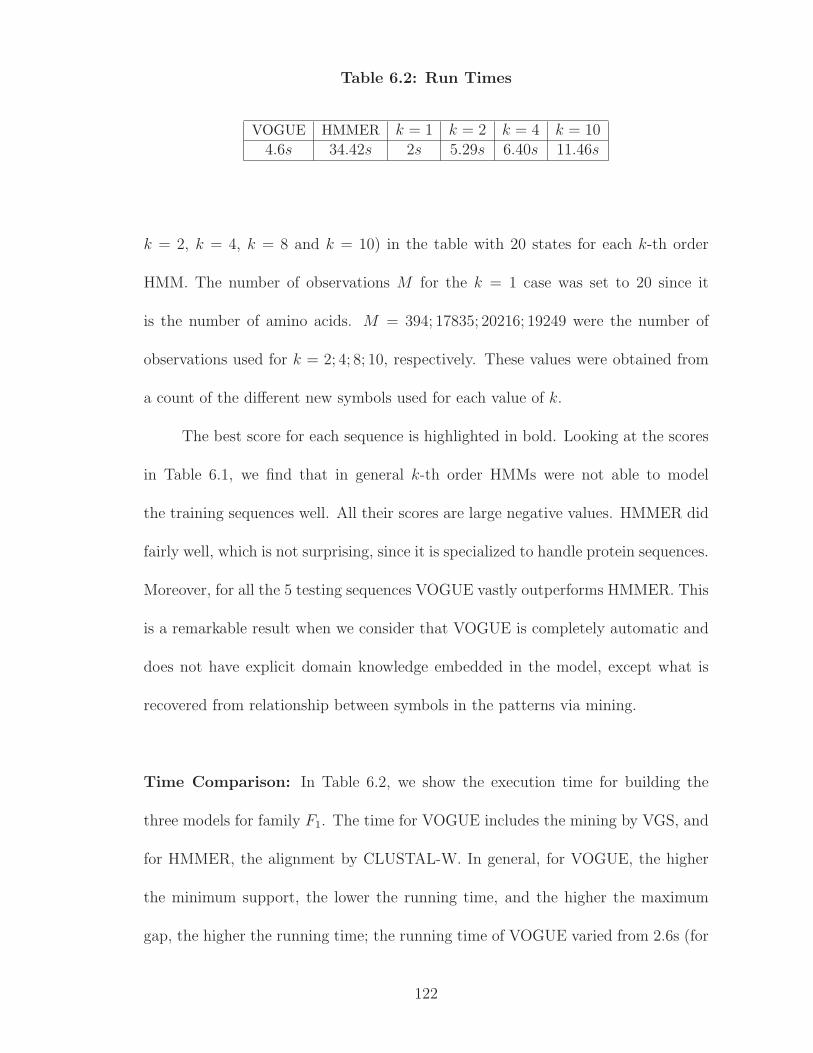
Table 6.2: Run Times
VOGUE HMMER k = 1 k = 2 k = 4 k = 104.6s 34.42s 2s 5.29s 6.40s 11.46s
k = 2, k = 4, k = 8 and k = 10) in the table with 20 states for each k-th order
HMM. The number of observations M for the k = 1 case was set to 20 since it
is the number of amino acids. M = 394; 17835; 20216; 19249 were the number of
observations used for k = 2; 4; 8; 10, respectively. These values were obtained from
a count of the different new symbols used for each value of k.
The best score for each sequence is highlighted in bold. Looking at the scores
in Table 6.1, we find that in general k-th order HMMs were not able to model
the training sequences well. All their scores are large negative values. HMMER did
fairly well, which is not surprising, since it is specialized to handle protein sequences.
Moreover, for all the 5 testing sequences VOGUE vastly outperforms HMMER. This
is a remarkable result when we consider that VOGUE is completely automatic and
does not have explicit domain knowledge embedded in the model, except what is
recovered from relationship between symbols in the patterns via mining.
Time Comparison: In Table 6.2, we show the execution time for building the
three models for family F1. The time for VOGUE includes the mining by VGS, and
for HMMER, the alignment by CLUSTAL-W. In general, for VOGUE, the higher
the minimum support, the lower the running time, and the higher the maximum
gap, the higher the running time; the running time of VOGUE varied from 2.6s (for
122
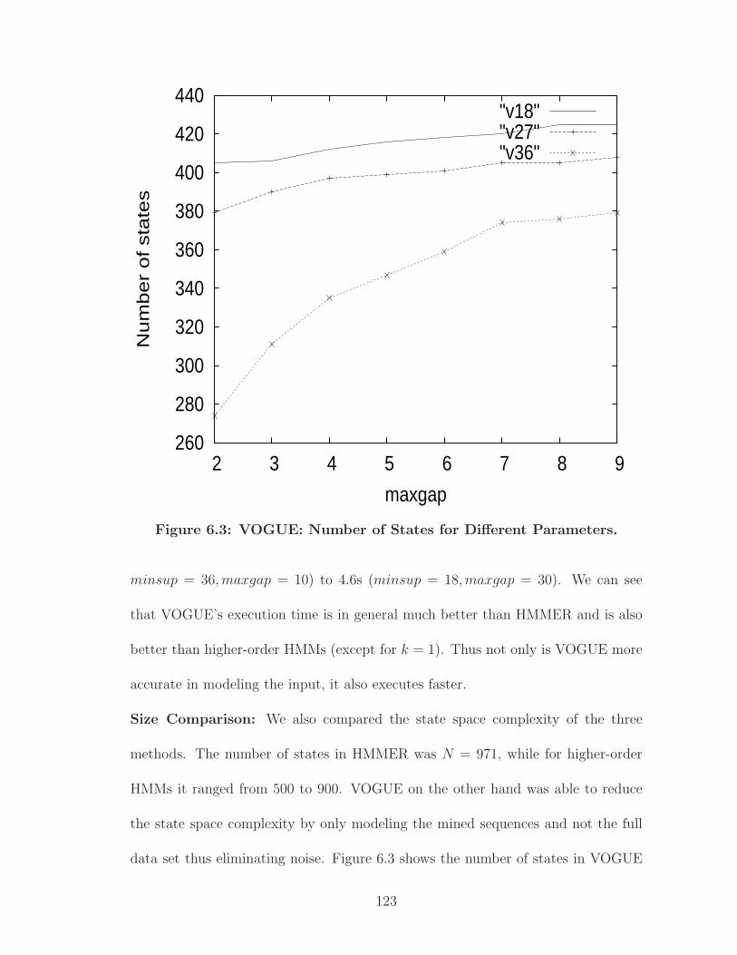
260
280
300
320
340
360
380
400
420
440
2 3 4 5 6 7 8 9
Nu
mb
er
of sta
tes
maxgap
"v18""v27""v36"
Figure 6.3: VOGUE: Number of States for Different Parameters.
minsup = 36,maxgap = 10) to 4.6s (minsup = 18,maxgap = 30). We can see
that VOGUE’s execution time is in general much better than HMMER and is also
better than higher-order HMMs (except for k = 1). Thus not only is VOGUE more
accurate in modeling the input, it also executes faster.
Size Comparison: We also compared the state space complexity of the three
methods. The number of states in HMMER was N = 971, while for higher-order
HMMs it ranged from 500 to 900. VOGUE on the other hand was able to reduce
the state space complexity by only modeling the mined sequences and not the full
data set thus eliminating noise. Figure 6.3 shows the number of states in VOGUE
123
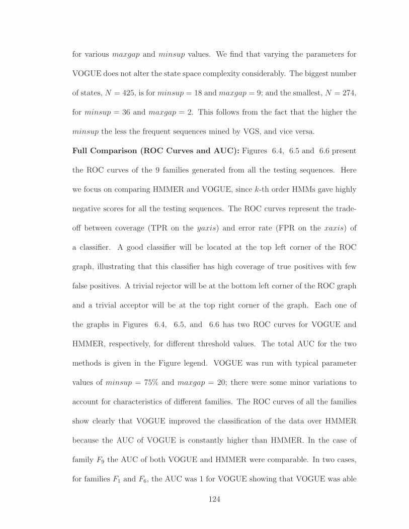
for various maxgap and minsup values. We find that varying the parameters for
VOGUE does not alter the state space complexity considerably. The biggest number
of states, N = 425, is for minsup = 18 and maxgap = 9; and the smallest, N = 274,
for minsup = 36 and maxgap = 2. This follows from the fact that the higher the
minsup the less the frequent sequences mined by VGS, and vice versa.
Full Comparison (ROC Curves and AUC): Figures 6.4, 6.5 and 6.6 present
the ROC curves of the 9 families generated from all the testing sequences. Here
we focus on comparing HMMER and VOGUE, since k-th order HMMs gave highly
negative scores for all the testing sequences. The ROC curves represent the trade-
off between coverage (TPR on the yaxis) and error rate (FPR on the xaxis) of
a classifier. A good classifier will be located at the top left corner of the ROC
graph, illustrating that this classifier has high coverage of true positives with few
false positives. A trivial rejector will be at the bottom left corner of the ROC graph
and a trivial acceptor will be at the top right corner of the graph. Each one of
the graphs in Figures 6.4, 6.5, and 6.6 has two ROC curves for VOGUE and
HMMER, respectively, for different threshold values. The total AUC for the two
methods is given in the Figure legend. VOGUE was run with typical parameter
values of minsup = 75% and maxgap = 20; there were some minor variations to
account for characteristics of different families. The ROC curves of all the families
show clearly that VOGUE improved the classification of the data over HMMER
because the AUC of VOGUE is constantly higher than HMMER. In the case of
family F9 the AUC of both VOGUE and HMMER were comparable. In two cases,
for families F1 and F6, the AUC was 1 for VOGUE showing that VOGUE was able
124
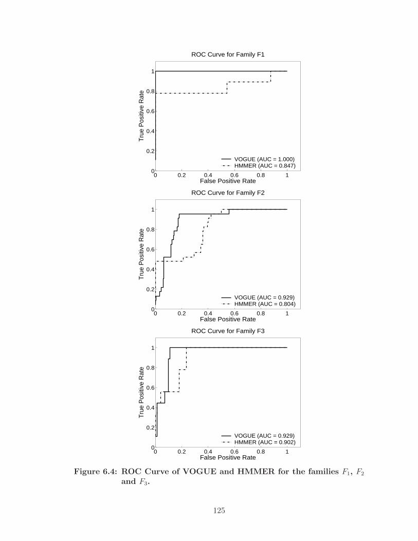
0 0.2 0.4 0.6 0.8 10
0.2
0.4
0.6
0.8
1
False Positive Rate
Tru
e P
ositi
ve R
ate
ROC Curve for Family F1
VOGUE (AUC = 1.000)HMMER (AUC = 0.847)
0 0.2 0.4 0.6 0.8 10
0.2
0.4
0.6
0.8
1
False Positive Rate
Tru
e P
ositi
ve R
ate
ROC Curve for Family F2
VOGUE (AUC = 0.929)HMMER (AUC = 0.804)
0 0.2 0.4 0.6 0.8 10
0.2
0.4
0.6
0.8
1
False Positive Rate
Tru
e P
ositi
ve R
ate
ROC Curve for Family F3
VOGUE (AUC = 0.929)HMMER (AUC = 0.902)
Figure 6.4: ROC Curve of VOGUE and HMMER for the families F1, F2
and F3.
125
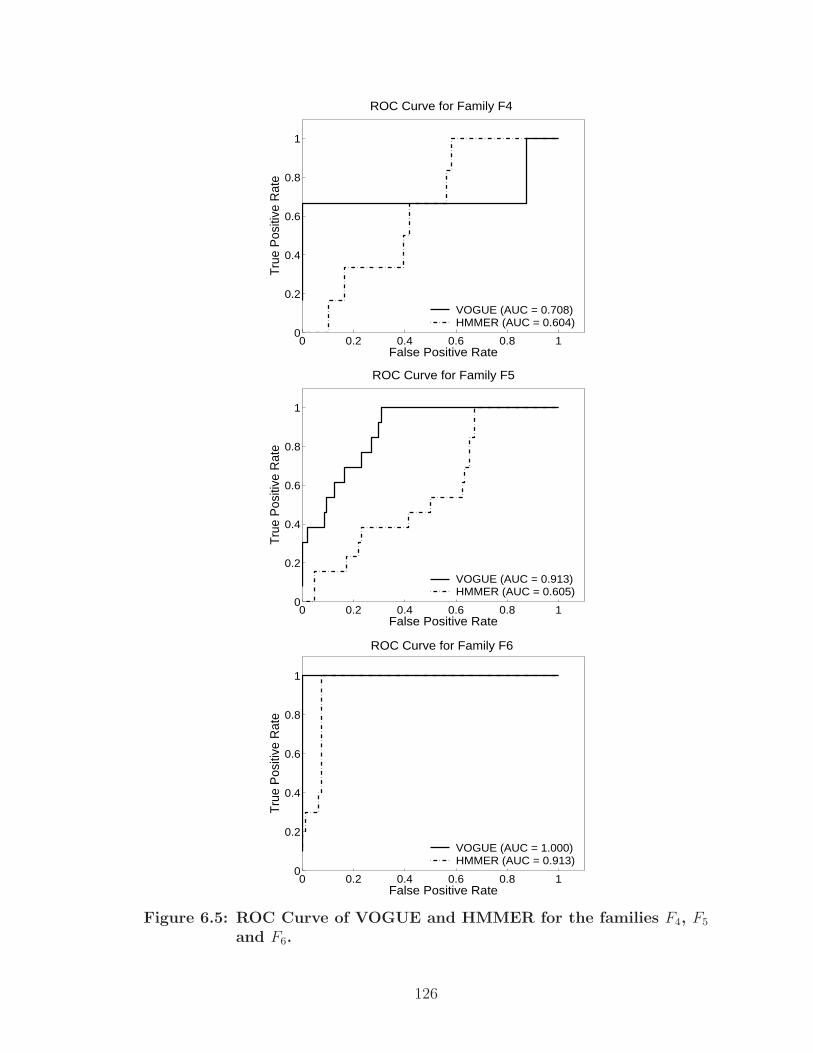
0 0.2 0.4 0.6 0.8 10
0.2
0.4
0.6
0.8
1
False Positive Rate
Tru
e P
ositi
ve R
ate
ROC Curve for Family F4
VOGUE (AUC = 0.708)HMMER (AUC = 0.604)
0 0.2 0.4 0.6 0.8 10
0.2
0.4
0.6
0.8
1
False Positive Rate
Tru
e P
ositi
ve R
ate
ROC Curve for Family F5
VOGUE (AUC = 0.913)HMMER (AUC = 0.605)
0 0.2 0.4 0.6 0.8 10
0.2
0.4
0.6
0.8
1
False Positive Rate
Tru
e P
ositi
ve R
ate
ROC Curve for Family F6
VOGUE (AUC = 1.000)HMMER (AUC = 0.913)
Figure 6.5: ROC Curve of VOGUE and HMMER for the families F4, F5
and F6.
126
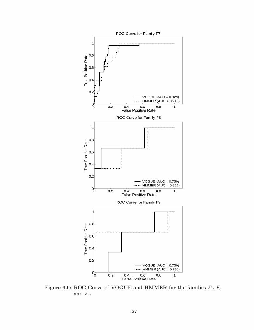
0 0.2 0.4 0.6 0.8 10
0.2
0.4
0.6
0.8
1
False Positive Rate
Tru
e P
ositi
ve R
ate
ROC Curve for Family F7
VOGUE (AUC = 0.929)HMMER (AUC = 0.913)
0 0.2 0.4 0.6 0.8 10
0.2
0.4
0.6
0.8
1
False Positive Rate
Tru
e P
ositi
ve R
ate
ROC Curve for Family F8
VOGUE (AUC = 0.750)HMMER (AUC = 0.629)
0 0.2 0.4 0.6 0.8 10
0.2
0.4
0.6
0.8
1
False Positive Rate
Tru
e P
ositi
ve R
ate
ROC Curve for Family F9
VOGUE (AUC = 0.750)HMMER (AUC = 0.750)
Figure 6.6: ROC Curve of VOGUE and HMMER for the families F7, F8
and F9.
127

to capture the patterns of those families perfectly. Moreover, in 6 out 9 families
the AUC for VOGUE was higher than 0.9 as opposed to HMMER whose AUC
was greater than 0.9 in only 3 out of 9 families. This again shows that VOGUE
outperforms HMMER.
6.3 Performance of VOGUE vs C-VOGUE vs HMMER on
PROSITE data
In this section, besides the models of VOGUE and HMMER from the previous
section, we also built a C-VOGUE state machine for the PROSITE data set. We
first run VGS on the training data set with different values of minsup corresponding
to 50%, 75% and 100% of the number of instances in the training data set, and
maxgap (10, 15, 20, 25, 30) but still with the constant k = 2 as the length of the
mined sequences by VGS. Then we prune the “artifacts” from the set of frequent
sequences and we build the new model C-VOGUE. We then choose the best set of
parameters, and fix them for the remaining of the experiments. We then compare
C-VOGUE to VOGUE and to HMMER. The results of C-VOGUE as opposed to
VOGUE and HMMER are shown in Figures 6.7, 6.8 and 6.9.
These figures show clearly that VOGUE’s and C-VOGUE’s ROC curves over-
lap for all 9 families, hence have the same AUC. Therefore, C-VOGUE also out-
performs HMMER. This experiments reinforces the claim that C-VOGUE keeps a
good coverage and an increased accuracy. Concerning the state space complexity,
Table 6.3 shows the number states using VOGUE and C-VOGUE for the 9 families.
128
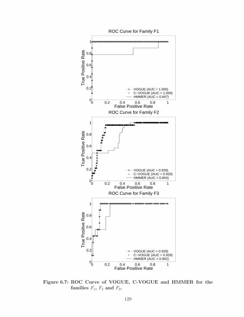
0 0.2 0.4 0.6 0.8 10
0.2
0.4
0.6
0.8
1
False Positive Rate
Tru
e P
ositi
ve R
ate
ROC Curve for Family F1
VOGUE (AUC = 1.000)C−VOGUE (AUC = 1.000)HMMER (AUC = 0.847)
0 0.2 0.4 0.6 0.8 10
0.2
0.4
0.6
0.8
1
False Positive Rate
Tru
e P
ositi
ve R
ate
ROC Curve for Family F2
VOGUE (AUC = 0.929)C−VOGUE (AUC = 0.929)HMMER (AUC = 0.804)
0 0.2 0.4 0.6 0.8 10
0.2
0.4
0.6
0.8
1
False Positive Rate
Tru
e P
ositi
ve R
ate
ROC Curve for Family F3
VOGUE (AUC = 0.929)C−VOGUE (AUC = 0.929)HMMER (AUC = 0.902)
Figure 6.7: ROC Curve of VOGUE, C-VOGUE and HMMER for thefamilies F1, F2 and F3.
129
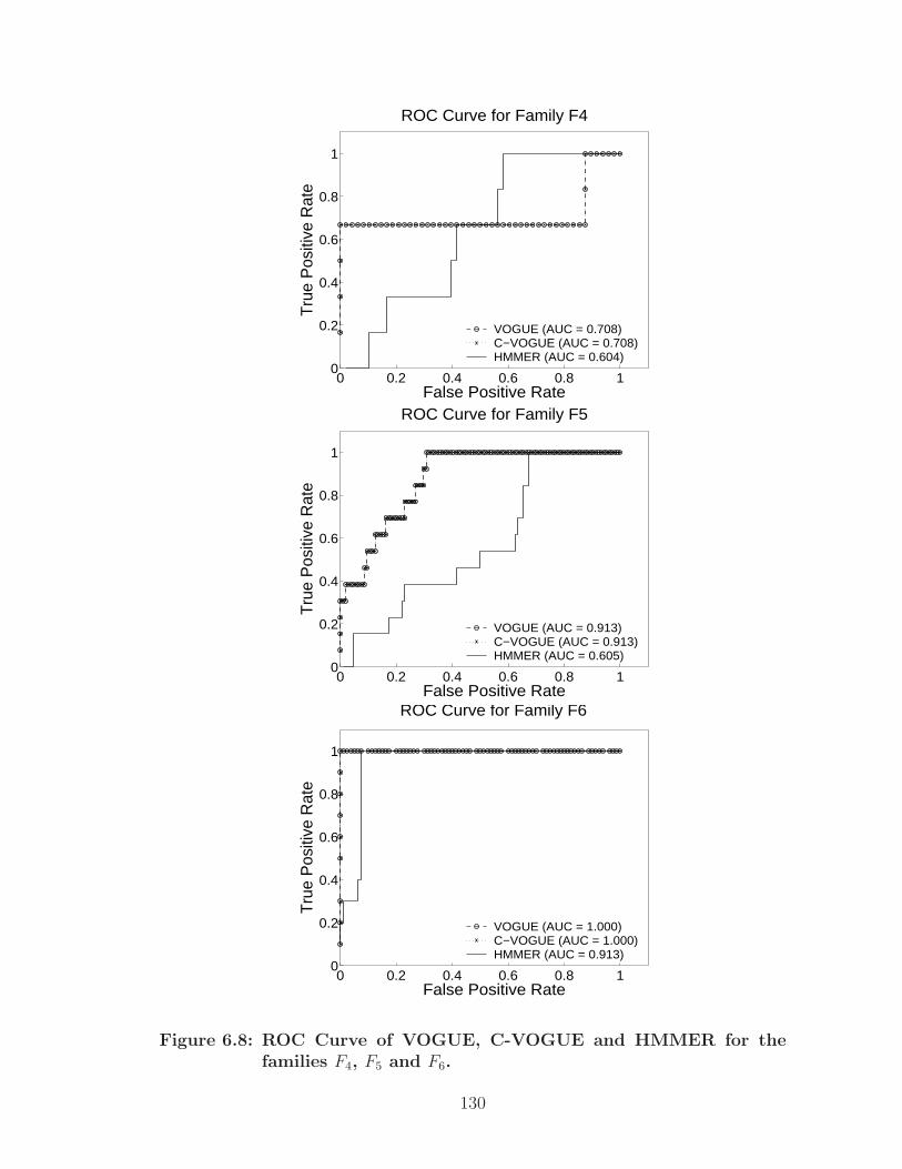
0 0.2 0.4 0.6 0.8 10
0.2
0.4
0.6
0.8
1
False Positive Rate
Tru
e P
ositi
ve R
ate
ROC Curve for Family F4
VOGUE (AUC = 0.708)C−VOGUE (AUC = 0.708)HMMER (AUC = 0.604)
0 0.2 0.4 0.6 0.8 10
0.2
0.4
0.6
0.8
1
False Positive Rate
Tru
e P
ositi
ve R
ate
ROC Curve for Family F5
VOGUE (AUC = 0.913)C−VOGUE (AUC = 0.913)HMMER (AUC = 0.605)
0 0.2 0.4 0.6 0.8 10
0.2
0.4
0.6
0.8
1
False Positive Rate
Tru
e P
ositi
ve R
ate
ROC Curve for Family F6
VOGUE (AUC = 1.000)C−VOGUE (AUC = 1.000)HMMER (AUC = 0.913)
Figure 6.8: ROC Curve of VOGUE, C-VOGUE and HMMER for thefamilies F4, F5 and F6.
130
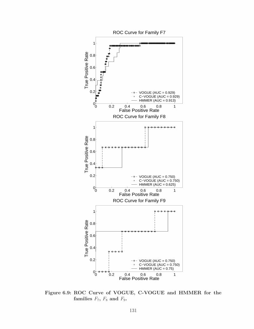
0 0.2 0.4 0.6 0.8 10
0.2
0.4
0.6
0.8
1
False Positive Rate
Tru
e P
ositi
ve R
ate
ROC Curve for Family F7
VOGUE (AUC = 0.929)C−VOGUE (AUC = 0.929)HMMER (AUC = 0.913)
0 0.2 0.4 0.6 0.8 10
0.2
0.4
0.6
0.8
1
False Positive Rate
Tru
e P
ositi
ve R
ate
ROC Curve for Family F8
VOGUE (AUC = 0.750)C−VOGUE (AUC = 0.750)HMMER (AUC = 0.625)
0 0.2 0.4 0.6 0.8 10
0.2
0.4
0.6
0.8
1
False Positive Rate
Tru
e P
ositi
ve R
ate
ROC Curve for Family F9
VOGUE (AUC = 0.750)C−VOGUE (AUC = 0.750)HMMER (AUC = 0.75)
Figure 6.9: ROC Curve of VOGUE, C-VOGUE and HMMER for thefamilies F7, F8 and F9.
131
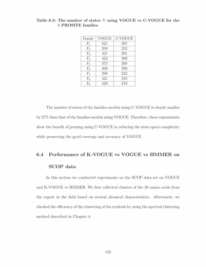
Table 6.3: The number of states N using VOGUE vs C-VOGUE for the9 PROSITE families
Family VOGUE C-VOGUE
F1 421 305F2 350 252F3 421 301F4 423 309F5 375 268F6 408 290F7 298 222F8 421 318F9 420 319
The number of states of the families models using C-VOGUE is clearly smaller
by 27% than that of the families models using VOGUE. Therefore, these experiments
show the benefit of pruning using C-VOGUE in reducing the state space complexity
while preserving the good coverage and accuracy of VOGUE.
6.4 Performance of K-VOGUE vs VOGUE vs HMMER on
SCOP data
In this section we conducted experiments on the SCOP data set on VOGUE
and K-VOGUE vs HMMER. We first collected clusters of the 20 amino acids from
the expert in the field based on several chemical characteristics. Afterwards, we
checked the efficiency of the clustering of the symbols by using the spectral clustering
method described in Chapter 4.
132
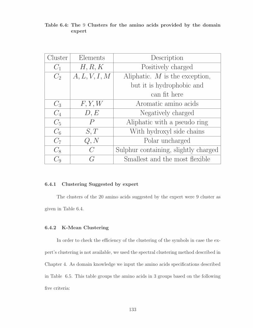
Table 6.4: The 9 Clusters for the amino acids provided by the domainexpert
Cluster Elements Description
C1 H, R, K Positively charged
C2 A, L, V, I, M Aliphatic. M is the exception,
but it is hydrophobic and
can fit here
C3 F, Y, W Aromatic amino acids
C4 D, E Negatively charged
C5 P Aliphatic with a pseudo ring
C6 S, T With hydroxyl side chains
C7 Q, N Polar uncharged
C8 C Sulphur containing, slightly charged
C9 G Smallest and the most flexible
6.4.1 Clustering Suggested by expert
The clusters of the 20 amino acids suggested by the expert were 9 cluster as
given in Table 6.4.
6.4.2 K-Mean Clustering
In order to check the efficiency of the clustering of the symbols in case the ex-
pert’s clustering is not available, we used the spectral clustering method described in
Chapter 4. As domain knowledge we input the amino acids specifications described
in Table 6.5. This table groups the amino acids in 3 groups based on the following
five criteria:
133
1. Hydrophobicity: an amino acid can be either polar, neutral or hydrophobic.
2. Polarity: if the polarity of an amino acid ranges from 4.9 to 6.2 it belongs to
the group 1, if it ranges from 8.0 to 9.2 it belongs to group 2 and if it ranges
from 10.0 to 13.0 it belongs to group 3.
3. Polarizability: If the polarizability of the amino acid ranges from 0 to 0.108
it belongs to the group 1, if it ranges from 0.128 to 0.180 it belongs to group
2 and if it ranges from 0.210 to 0.409 it belongs to group 3.
4. Charge: an amino acid could be either positive, negative or carrying a small
charge or no charge, called other.
5. Normalized Van Derwaals volume: if the volume of the amino acid ranges
from 0 to 2.8 it belongs to the group 1, if it ranges from 2.95 to 4.0 it belongs
to group 2 and if it ranges from 4.43 to 8.08 it belongs to group 3.
We used K-means with different values of the number of clusters K(5, 6, 7, 9).
The best results of the clustering was for K = 9 and is shown in Figure 6.10. The X
axis represents the K eigenvectors that correspond to the K largest eigenvalues. The
last column represents the cluster index in color to which the amino acid belongs
to. The Y axis represents the amino acid index. The amino acids indexes are
represented from 1 to 20 as described in Table 6.6.
Clustering using the spectral clustering using eigenvectors and K-means with
K = 9, we obtained the following 9 clusters as described in Table 6.7.
134
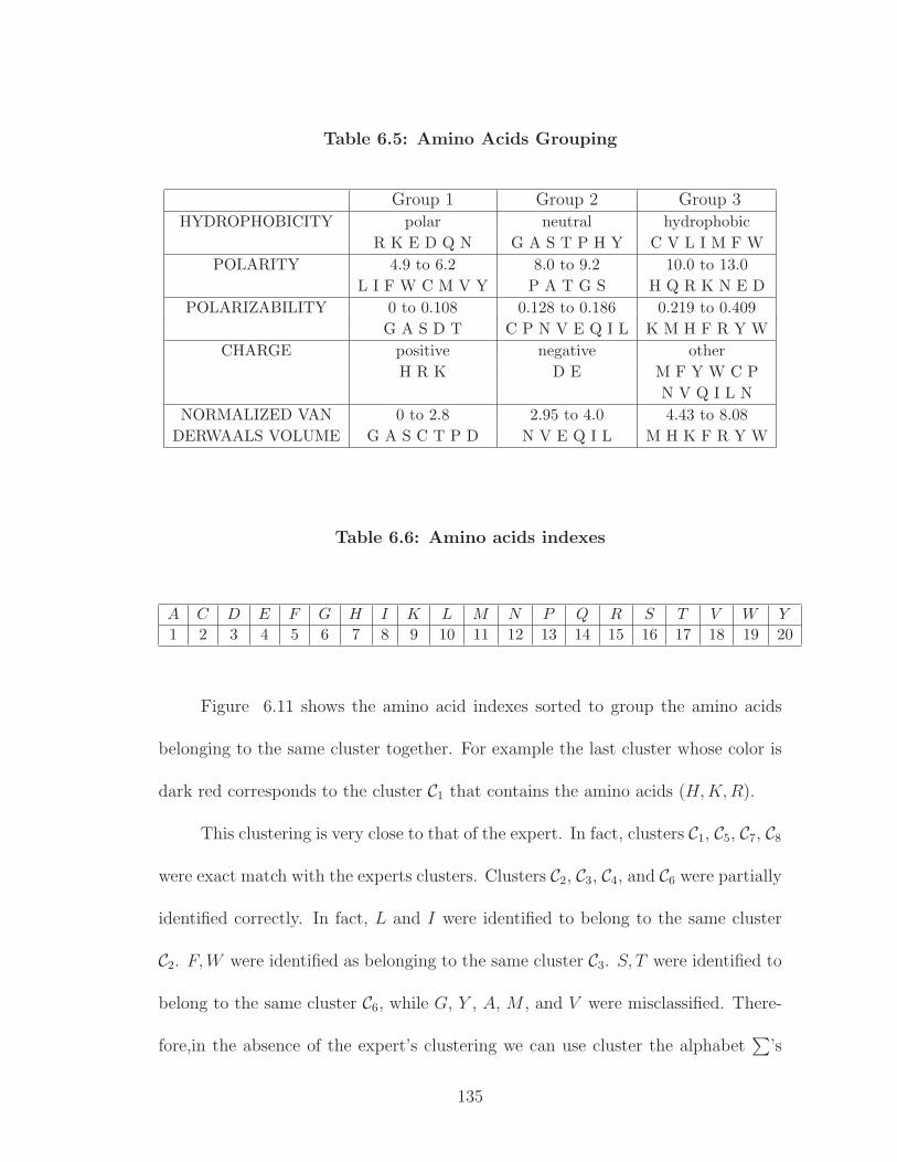
Table 6.5: Amino Acids Grouping
Group 1 Group 2 Group 3HYDROPHOBICITY polar neutral hydrophobic
R K E D Q N G A S T P H Y C V L I M F W
POLARITY 4.9 to 6.2 8.0 to 9.2 10.0 to 13.0
L I F W C M V Y P A T G S H Q R K N E D
POLARIZABILITY 0 to 0.108 0.128 to 0.186 0.219 to 0.409
G A S D T C P N V E Q I L K M H F R Y W
CHARGE positive negative other
H R K D E M F Y W C P
N V Q I L N
NORMALIZED VAN 0 to 2.8 2.95 to 4.0 4.43 to 8.08
DERWAALS VOLUME G A S C T P D N V E Q I L M H K F R Y W
Table 6.6: Amino acids indexes
A C D E F G H I K L M N P Q R S T V W Y
1 2 3 4 5 6 7 8 9 10 11 12 13 14 15 16 17 18 19 20
Figure 6.11 shows the amino acid indexes sorted to group the amino acids
belonging to the same cluster together. For example the last cluster whose color is
dark red corresponds to the cluster C1 that contains the amino acids (H,K,R).
This clustering is very close to that of the expert. In fact, clusters C1, C5, C7, C8
were exact match with the experts clusters. Clusters C2, C3, C4, and C6 were partially
identified correctly. In fact, L and I were identified to belong to the same cluster
C2. F,W were identified as belonging to the same cluster C3. S, T were identified to
belong to the same cluster C6, while G, Y , A, M , and V were misclassified. There-
fore,in the absence of the expert’s clustering we can use cluster the alphabet∑
’s
135
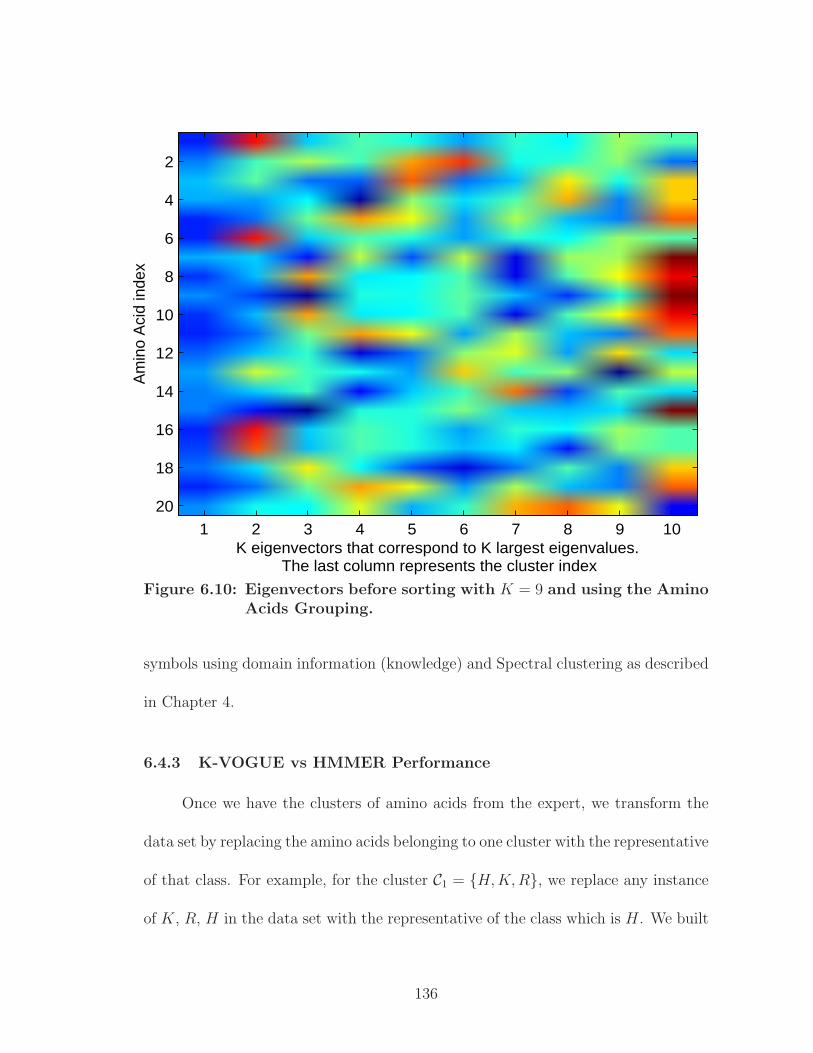
Am
ino
Aci
d in
dex
K eigenvectors that correspond to K largest eigenvalues. The last column represents the cluster index
1 2 3 4 5 6 7 8 9 10
2
4
6
8
10
12
14
16
18
20
Figure 6.10: Eigenvectors before sorting with K = 9 and using the AminoAcids Grouping.
symbols using domain information (knowledge) and Spectral clustering as described
in Chapter 4.
6.4.3 K-VOGUE vs HMMER Performance
Once we have the clusters of amino acids from the expert, we transform the
data set by replacing the amino acids belonging to one cluster with the representative
of that class. For example, for the cluster C1 = {H,K,R}, we replace any instance
of K, R, H in the data set with the representative of the class which is H. We built
136
Table 6.7: The 9 Clusters for the amino acids from K-means clustering
Cluster Elements Indexes of elements
C1 H, K, R (7, 9, 15)
C2 I, L (8, 10)
C3 F, M, W (5, 11, 19)
C4 D, E, V (3, 4, 18)
C5 P (13)
C6 A, G, S, T (1, 6, 16, 17)
C7 N, Q (12, 14)
C8 C (2)
C9 (Y ) (20)
K-VOGUE state machines with different values of minsup corresponding to 50%,
75% and 100% of the number of instances in the training data, and maxgap (10,
15, 20, 25, 30) but with the constant k = 2 for the length of the mined sequences
in VGS. We then choose the best set of parameters and fix them for the remaining
experiments. To model the data using HMMER, we first align the training sequences
using CLUSTAL-W (http://www.ebi.ac.uk/clustalw). We then build a profile
HMM using the multiple sequence alignment and compute the scores for each test
sequence using HMMER, which directly reports the log-odds scores with respect to
the Null model mentioned above.
Score Comparison: We first compare K-VOGUE HMMER. Table 6.8 shows the
comparison on the 10 testing sequences from all the 10 families when scored against
the model for families SF2 and SF5. For K-VOGUE we used minsup = 6(75%) and
maxgap = 20.
137
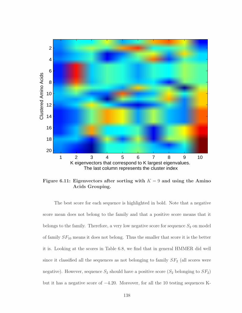
Clu
ster
ed A
min
o A
cids
K eigenvectors that correspond to K largest eigenvalues. The last column represents the cluster index
1 2 3 4 5 6 7 8 9 10
2
4
6
8
10
12
14
16
18
20
Figure 6.11: Eigenvectors after sorting with K = 9 and using the AminoAcids Grouping.
The best score for each sequence is highlighted in bold. Note that a negative
score mean does not belong to the family and that a positive score means that it
belongs to the family. Therefore, a very low negative score for sequence S2 on model
of family SF10 means it does not belong. Thus the smaller that score it is the better
it is. Looking at the scores in Table 6.8, we find that in general HMMER did well
since it classified all the sequences as not belonging to family SF2 (all scores were
negative). However, sequence S2 should have a positive score (S2 belonging to SF2)
but it has a negative score of −4.20. Moreover, for all the 10 testing sequences K-
138
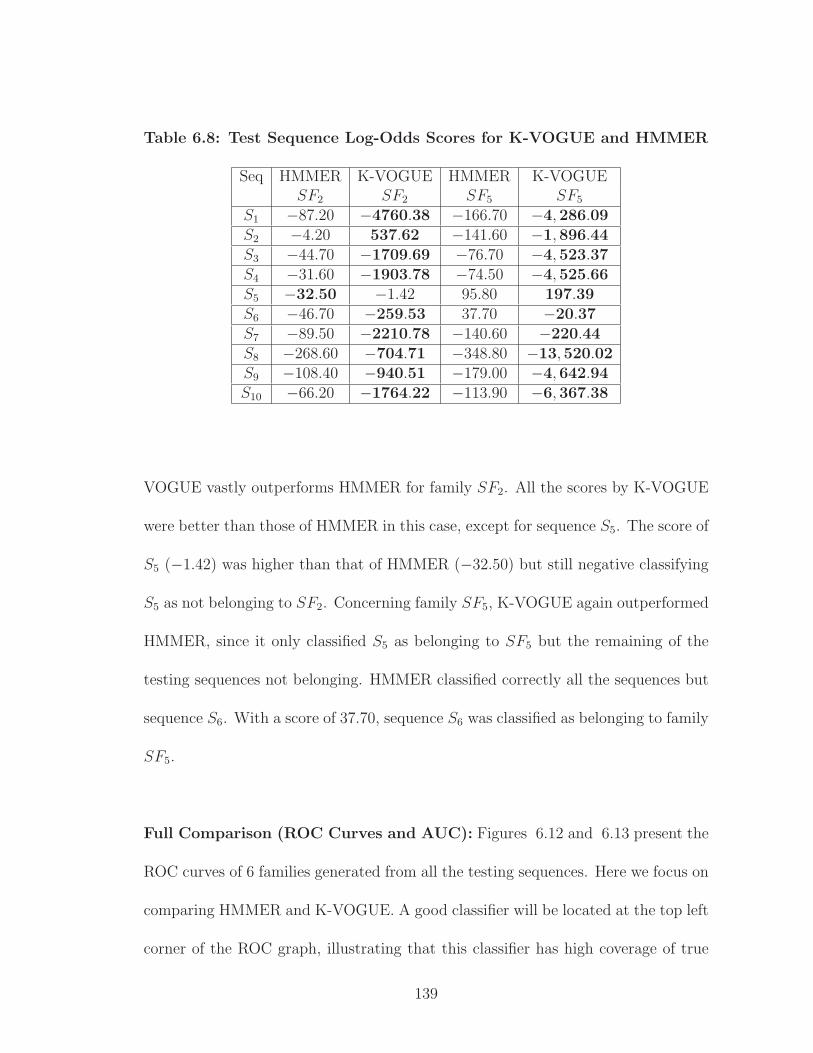
Table 6.8: Test Sequence Log-Odds Scores for K-VOGUE and HMMER
Seq HMMER K-VOGUE HMMER K-VOGUESF2 SF2 SF5 SF5
S1 −87.20 −4760.38 −166.70 −4,286.09S2 −4.20 537.62 −141.60 −1,896.44S3 −44.70 −1709.69 −76.70 −4,523.37S4 −31.60 −1903.78 −74.50 −4,525.66S5 −32.50 −1.42 95.80 197.39S6 −46.70 −259.53 37.70 −20.37S7 −89.50 −2210.78 −140.60 −220.44S8 −268.60 −704.71 −348.80 −13,520.02S9 −108.40 −940.51 −179.00 −4,642.94S10 −66.20 −1764.22 −113.90 −6,367.38
VOGUE vastly outperforms HMMER for family SF2. All the scores by K-VOGUE
were better than those of HMMER in this case, except for sequence S5. The score of
S5 (−1.42) was higher than that of HMMER (−32.50) but still negative classifying
S5 as not belonging to SF2. Concerning family SF5, K-VOGUE again outperformed
HMMER, since it only classified S5 as belonging to SF5 but the remaining of the
testing sequences not belonging. HMMER classified correctly all the sequences but
sequence S6. With a score of 37.70, sequence S6 was classified as belonging to family
SF5.
Full Comparison (ROC Curves and AUC): Figures 6.12 and 6.13 present the
ROC curves of 6 families generated from all the testing sequences. Here we focus on
comparing HMMER and K-VOGUE. A good classifier will be located at the top left
corner of the ROC graph, illustrating that this classifier has high coverage of true
139
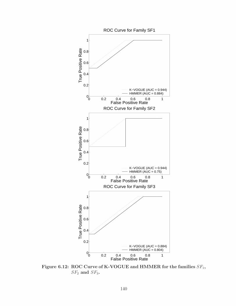
0 0.2 0.4 0.6 0.8 10
0.2
0.4
0.6
0.8
1
False Positive Rate
Tru
e P
ositi
ve R
ate
ROC Curve for Family SF1
K−VOGUE (AUC = 0.944)HMMER (AUC = 0.884)
0 0.2 0.4 0.6 0.8 10
0.2
0.4
0.6
0.8
1
False Positive Rate
Tru
e P
ositi
ve R
ate
ROC Curve for Family SF2
K−VOGUE (AUC = 0.944)HMMER (AUC = 0.75)
0 0.2 0.4 0.6 0.8 10
0.2
0.4
0.6
0.8
1
False Positive Rate
Tru
e P
ositi
ve R
ate
ROC Curve for Family SF3
K−VOGUE (AUC = 0.884)HMMER (AUC = 0.804)
Figure 6.12: ROC Curve of K-VOGUE and HMMER for the families SF1,SF2 and SF3.
140
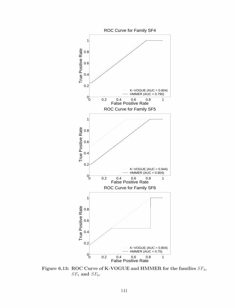
0 0.2 0.4 0.6 0.8 10
0.2
0.4
0.6
0.8
1
False Positive Rate
Tru
e P
ositi
ve R
ate
ROC Curve for Family SF4
K−VOGUE (AUC = 0.804)HMMER (AUC = 0.790)
0 0.2 0.4 0.6 0.8 10
0.2
0.4
0.6
0.8
1
False Positive Rate
Tru
e P
ositi
ve R
ate
ROC Curve for Family SF5
K−VOGUE (AUC = 0.944)HMMER (AUC = 0.804)
0 0.2 0.4 0.6 0.8 10
0.2
0.4
0.6
0.8
1
False Positive Rate
Tru
e P
ositi
ve R
ate
ROC Curve for Family SF6
K−VOGUE (AUC = 0.804)HMMER (AUC = 0.75)
Figure 6.13: ROC Curve of K-VOGUE and HMMER for the families SF4,SF5 and SF6.
141
positives with few false positives. A trivial rejector will be at the bottom left corner
of the ROC graph and a trivial acceptor will be at the top right corner of the graph.
Each one of the graphs in Figures 6.12, 6.13 has two ROC curves for K-VOGUE
and HMMER, respectively, for different threshold values. The total AUC for the
two methods is given in the legend. K-VOGUE was run with parameter typical
values of minsup = 75% and maxgap = 20; there were some minor variations to
account for characteristics of different families. The ROC curves of all the families
show clearly that VOGUE improved the classification of the data over HMMER
because the AUC of VOGUE is constantly higher than HMMER.
6.5 Summary
In this Chapter, we conducted several experiments on real data sets from the
PROSITE and SCOP data sets. We compared the performance of VGOUE to that of
HMMER and higher-order HMM on the PROSITE data set. The results proved that
VOGUE has a higher prediction power and accuracy over HMMER and higher-order
HMM while keeping a relatively low state complexity. Moreover, we conducted simi-
lar experiments using C-VOGUE and we found that C-VOGUE’s results are similar
to those of VOGUE while reducing the latter’s state space complexity even fur-
ther. Finally, we compared the performance of K-VOGUE and HMMER on SCOP
data set. The results showed that K-VOGUE outperformed HMMER. Therefore,
VOGUE and its variations are a good modeling tool that increase the accuracy and
prediction while reducing the state space complexity.
142
Chapter 7Conclusions and Future
Work
We introduced a new state machine called VOGUE to discover and interpret tem-
poral dependencies in the analyzed data. We formally defined the two steps of this
technique, where the first step uses a new and efficient sequence mining algorithm,
Variable-Gap Sequence mining (VGS), to mine frequent patterns, and the second
step uses these mined sequences to build VOGUE. An important contribution of
our new technique is that we are able to simultaneously model multiple higher-order
HMMs due to the inclusion of variable length gaps allowed in the mined sequences.
Once the model is built, it can be used to interpret new observation sequences. Ther-
fore, we modified the widely used Viterbi algorithm into VG-Viterbi, to take into
consideration the special topology of VOGUE. We showed experimentally, using real
protein sequence data, that VOGUE’s modeling power is superior to higher-order
HMMs, as well as a domain-specific algorithm HMMER.
We further generalized VOGUE to any length, k ≥ 2, of the sequences mined
by VGS. Furthermore, some patterns mined by VGS are artifacts of other patterns,
for example, if A → B is frequent, then there is a good chance that B → A will be
143
frequent as well. We developed a special pruning mechanism, called, C-VOGUE, to
separate primary patterns from artifacts.We showed through experimental results
that, C-VOGUE reduces further the state space complexity of VOGUE while main-
taining a good coverage and accuracy. Moreover, there are applications where there
isn’t always an exact match for the subsequences to be mined, such as in bioinfor-
matics or in user data access. We extended VOGUE to K-VOGUE, to allow for
approximate matches for the mined sequences and states. K-VOGUE takes into
consideration that some elements in the alphabet Σ share similar characteristics
and hence are similar. These elements are clustered either by a domain expert or
by using domain information and spectral clustering as clustering technique. Then,
VGS looks for frequent patterns whose elements belong to the same cluster instead
of an exact match between the elements.
We used pseudo-counts in the transition, emission and duration probabilities,
to account for the symbols that were not present in the training data set but might be
present in the testing data sets. The values of these pseudo-counts were heuristically
chosen but they were fixed for all the symbols. We need to automate this process
and allow for pseudo-count values that reflect the overall distribution of the symbols.
In fact, a symbol might have higher occurrences than others and hence its pseudo-
count should be higher. Moreover, we need to understand what is the impact of the
chosen pseudo-count value on the performance of VOGUE.
We showed that VOGUE and its variations were able to outperform the state-
of-the-art techniques in biological sequence clustering and analysis. VOGUE can
be further used in other applications such as user access behavior [2], web prefetch-
144

ing [8], security [84], and many more interesting and challenging real world problems.
145
LITERATURE CITED
[1] K. Aas, L. Eikvil, and T. Andersen. Text recognition from grey level imagesusing hidden Markov models. Lecture Notes in Computer Science, 970, 1995.
[2] S. Adali, B. Bouqata, A. Marcus, B. Szymanski, and F. Spear. A day in thelife of a metamorphic petrologist. 22nd Int’l Conf. on Data Engineering, 2006.
[3] R. Agrawal, H. Mannila, R. Srikant, H. Toivonen, and A. Verkamo. Fast dis-covery of association rules. In Fayyad, U., and al. eds., Advances in KnowledgeDiscovery and Data Mining. AAAI Press, Menlo Park, CA, 1998.
[4] R. Agrawal and R. Srikant. Fast algorithms for mining association rules. 20thIntl. Conf. Very Large Databases (VLDB)., September 1994.
[5] R. Agrawal and R. Srikant. Mining sequential patterns. 11th IDE Conf., 1995.
[6] C. Antunes and A. L. Oliveira. Generalization of pattern-growth methodsfor sequential pattern mining with gap constraints. Machine Learning andData Mining in Pattern Recognition, Springer LNCS Vol. 2734, pages 239–251, 2003.
[7] S. F. Atschul. Amino acid substitution matrices from an information theoreticsperspective. Molecular Biology, 219:555–665, 1991.
[8] Bouqata B., Carothers C., Szymanski B., and Zaki M. Understading filesystemperformance for data mining applications. Proceedings of the 6th InternationalWorkshop on High Performance Data Mining: Pervasive and Data StreamMining (HPDM:PDS‘03), 2003.
[9] R. Bakis. Continuous speech word recognition via centi-second acoustic states.Proc. ASA Meeting (Washintong DC), 1976.
[10] P. Baldi, Y. Chauvin, T. Hunkapiller, and M. McClure. Hidden markov modelsof biological primary sequence information. Proc. Nat’l Academy of Sciences,91:1059–1063, Feb. 1994.
[11] L. E. Baum. An inequality and associated maximization technique in statis-tical estimation for probabilistic functions of markov processes. Inequalities,pages 1–8, 1972.
146
[12] L. E. Baum and J. Egon. An inequality with applications to statistical estima-tion for probabilistic functions of markov process and to a model for ecology.Bull. Amer. Meteorol. Soc., pages 360–363, 1967.
[13] L. E. Baum and T. Petrie. Statistical inference for probabilistic functions offinite state markov chains. Ann. Math. Stat., pages 1554–1563, 1966.
[14] L. E. Baum, T. Petrie, G. Soules, and N. Weiss. A maximization techniqueoccurring in the statistical analysis of probabilistic functions of markov chains.Ann. Math. Stat., (1):164–171, 1970.
[15] L. E. Baum and G. R. Sell. Growth functions for transformations on manifolds.Pacif. J. Math., (2):211–227, 1968.
[16] G. Bernardi, B. Olofsson, J. Filipski, M. Zerial, J. Salinas, G. Curry,M. Meunier-Rotival, and F. Rodier. The mosaic genome of warm-bloodedvertebrates. Science, 228(4702):953–958, 1985.
[17] C. Bettini, X.S. Wang, S. Jajodia, and J.L. Lin. Discovering frequent eventpatterns with multiple granularities in time sequences. IEEE Transactions onKnowledge and Data Engineering, 10(2):222–237, March 1998.
[18] M. P. Brown, R. Hughey, A. Krogh, I. S. Mian, K. Sjolander, and D. Haussler.Using dirichlet mixture priors to derive hidden markov models for proteinfamilies. pages 47–55, 1993.
[19] M. Brudno, S. Malde, A. Poloakov, C. B. Do, O. Couronne, I. Dubchak, andS. Batzoglou. Global alignment finding rearrangements during alignment.Bioinformatics, 19(1):54–62, 2003.
[20] L. Lo Conte, S. E. Brenner, T. J. P. Hubbard, C. Chothia, and A. G. Murzin.Scop database in 2002: refinement accommodate structural genomics. NucleicAcids Res., 30:264–267, 2002.
[21] E. Coward and F. Drablos. Detecting periodic patterns in biological sequences.Bioinformatics, Oxford university press, 14:498–507, 1998.
[22] B. A. Davey and H. A. Priestley. Introduction to lattices and order. CambridgeUniversity Press, 1990.
[23] M. Deshpande and G. Karypis. Selective markov models for predicting web-page accesses. April 2001.
[24] C. H. Q. Ding and I. Dubchak. Multi-class protein fold recognition usingsupport vector machines and neural networks. Bioinformatics., 17:349–358,2001.
[25] R. F. Doolittle. Redundancies in protein sequences. In Predictions of Pro-tein Structure and the Principles of Protein Conformation (Fasman, G.D. ed)Plenum Press, New York, pages 599–623, 1989.
147

[26] J.A. du Preez. Efficient training of high-order hidden markov models usingfirst-order representation. Computer Speech and Language, 12(1):23–39, 1998.
[27] R. Durbin, S. Eddy, A. Krogh, and G. Mitchison. Biological Sequence Analysis:Probabilistic nodels for proteins and nucleic acids. Cambridge Univ. Press,1998.
[28] R. Eddy. Where did the blosum62 alignment score matrix come from?. Nat.Biotechnology, 22(8):1035–6, 2004.
[29] S. R. Eddy. Hidden markov models. Current Opinion in Structural Biology,6:361–365, 1996.
[30] S. R. Eddy. Profile hidden markov models. Bioinformatics, 14:755–763, 1998.
[31] H. A. Edelstein. Introduction to data mining and knowledge discovery (3rded). Two Crows Corp, Potomac, MD, 1999.
[32] E. S. Lander et al. Initial sequencing and analysis of the human genome.Nature, 409(6822):860–921, 2001.
[33] J. C. Venter et al. The sequence of the human genome. Science,291(5507):1304–1351, 2002.
[34] P.F. Evangelista, M.J. Embrechts, P. Bonissone, and B. K. Szymanski. Fuzzyroc curves for unsupervised nonparametric ensemble techniques. InternationalJoint Conference on Neural Networks (IJCNN’05), 5:3040–3045, 2005.
[35] U. M. Fayyad, G. Piatetsky-Shapiro, P. Smyth, and R. Uthurusamy. Advancesin knowledge discovery and data mining. MIT Press., Cambridge, MA, 1996.
[36] P. Felzenszwalb, D. Huttenlocher, and J. Kleinberg. Fast algorithms for large-state-space hmms with applications to web usage analysis. In Advances inNeural Information Processing Systems, 2003.
[37] P. G. Ferreira and P. J. Azevedo. Protein sequence classification throughrelevant sequence mining and bayes classifiers. Springer-Verlag, 2005.
[38] J. W. Fickett and C.-S. Tung. Assessment of protein coding measures. NucleicAcids Research, 20(24):6441–6450, 1992.
[39] G. D. Forney. The viterbi algorithm. Proc. IEEE, 61:268–278, March 1973.
[40] W. Frawley, G. Piatetsky-Shapiro, and C. Matheus. Knowledge discovery indatabases: An overview. AI Magazine, pages 213–228, Fall 1992.
[41] Y. Fujiwara, M. Asogawa, and A. Konagaya. Stochastic motif extraction usinghidden markov model. pages 121–129. AAAI Press, 1994.
148
[42] M. Garofalakis, R.Rastogi, and K. Shim. Spirit: Sequential pattern miningwith regular expression constraints. In 25th Intl. Conf. VEry Large Databases,1999.
[43] M. Garofalakis, R.Rastogi, and K. Shim. Mining sequential patterns withregular expression constraints. IEEE TKDE, 14:530–552, May 2002.
[44] J. Han and M. Kamber. Data mining: Concepts and Techniques. Morgan-Kaufman, New York, NY, 2000.
[45] D. Hand, H. Mannila, and P. Smyth. Principles of Data Mining. MIT Press,Cambridge, MA, 2001.
[46] T. Hastie, R. Tibshirani, and J. H. Friedman. The elements of statisticallearning : Data mining, inference, and prediction. Springer, New York, NY,2001.
[47] K. Hatonen, M. Klemettinen, H. Mannila, P. Ronkainen, and H. Toivonen.Knowledge discovery from telecommunication network alarm databases. 12thIntl. Conf. Data Engineering, February 1996.
[48] L. S. Ho and J. C. Rajapakse. Splice site detection with higher-order markovmodel implemented on a neural network. Genome Informatics, 14:64–72, 2003.
[49] M. Holsheimer, M. Kersten, H. Mannila, and H. Toivonen. A perspective ondatabases and data mining. Proc. of 1st Intl. Conf. on knowledge Discoveryand Data Mining (KDD), August 1995.
[50] F. Jelinek. Continous speech recognition by statistical methods. volume 64,pages 532–536, 1976.
[51] R. Kannan, S. Vempala, and A. Vetta. On clusterings - good, bad, and spec-tral. In Proc. of the 41st Annual Symposium on Foundations of ComputerScience, 2000.
[52] T. Kanungo. Stochastic language models for style-directed layout analysis ofdocument images. IEEE Transactions on Image Processing, 12(5), May 2003.
[53] M. Klemettinen, H. Mannila, P. Ronkainen, H. Toivonen, and A. I. Verkamo.Finding interesting rules from large sets of discovered association rules. In 3rdIntl. Conf. Information and Knowledge Management,, pages 401–407, Novem-ber 1994.
[54] S. Koenig, R. Goodwin, and R. Simmons. Robot navigation with markov mod-els: A framework for path planning and learning with limited computationalresources. December 1995.
[55] S. Kurtz, J. V. Choudhuri, E. Ohlebusch, C. Schleiermacher, J. Stoye, andR. Giegerich. Reputer: the manifold applications of repeat analysis on a gen-emic scale. Nucleic Acids Research, 29(22):4633–4642, 2001.
149
[56] S.E. Levinson. Structural methods in automatic speech recognition. volume73 (11), pages 1625–1650, 1985.
[57] S.E. Levinson. Continuously variable duration hidden markov models for au-tomatic speech recognition. volume 1 (1), pages 29–45, 1986.
[58] S.E. Levinson, L. R. Rabiner, and M. M. Sondhi. An introduction to theapplication of the theory of probabilistic functions of a markov process toautomatic speech recognition. Bell Syst. Tech. Journal, 62(4):1035–1074, 1983.
[59] C. Liebecq. Biochemical Nomenclature and Related Documents. 2d Edition.Portland Press.
[60] J. Lin, E.Keogh, S. Lonardi, and P. Patel. Finding motifs in time series.Temporal Data Mining Workshop Notes and K.P. Unnikrishnan and R. Uthu-rusamy and eds, July 2002.
[61] B. Lowerre and R. Reddy. The harpy speech understanding system. pages340–346. W. Lea, Editor. Englewood Cliffs,NJ: Prentice-Hall, 1980.
[62] H. Mannila and H. Toivonen. Discovering generalized episodes using minimaloccurences. 2d Intl. Conf. Knowledge Discover and Data Mining, 1996.
[63] H. Mannila, H. Toivonen, and I. Verkamo. Discovery of frequent episodes inevent sequences. Data Mining and Knowledge Discovery: An internationalJournal,, 1(3):259–289, 1997.
[64] D. Meyer. Human Gait Classification Based on Hidden Markov Models. pages139–146, 1997.
[65] D. M. Mount. Bioinformatics: Sequence and genome analysis 2nd ed. ColdSpring Harbor Laboratory Press: Cold Spring Harbor, NY, 2004.
[66] A. Nanopoulos, D. Katsaros, and Y. Manolopoulos. A data mining algorithmfor generalized web prefetching. IEEE Transactions on Knowledge and DataEngineering, 15(5):1155–1169, 2003.
[67] A. Y. Ng, M. Jordan, and Y. Weiss. On spectral clustering: Analysis and analgorithm. In Proc. of the NIPS-14, 2001.
[68] R. T. Ng, L. V. S. Lakshmanan, and J. Han. Exploratory mining and pruningoptimizations of constrained association rules. In ACM SIGMOD Intl. Conf.Management of Data,, June 1998.
[69] C. Notredame. Recent progresses in multiple sequence alignement: a survey.Pharmacogenomics (2002), 3(1).
[70] T. Oates, M. D. Schmill, D Jensen, and P. R. Cohen. A family of algorithmsfor finding temporal structure in data. In 6th Intl. Workshop on AI andStatistics,, March 1997.
150
[71] J. S. Pedersen and J. Hein. Gene finding with a hidden markov model ofgenome structure and evolution. Bioinfromatics, 19(2):219–227, 2003.
[72] J. Pei, J. Han, B. Mortazavi-Asl, H. Pinto, Q. Chen, U. Dayal, and M-C. Hsu.Prefixspan: Mining sequential patterns efficiently by prefix projected patterngrowth. April 2001.
[73] P. Pirolli and J. E. Pitkow. Distribution of surfers paths through the worldwide web: Empirical characterization. volume 2(1-2), pages 29–45, 1999.
[74] J. Pitkow and P. Pirolli. Mining longest repeating subsequence to predictWWW surfing. 1999.
[75] L.R. Rabiner. A tutorial on hidden markov models and selected applicationsin speech recognition. Proceedings IEEE, 2(77):257–286, 1989.
[76] P. S. Reddy and D. E. Housman. The complex pathology of trinucleotiderepeats. Current Opin. Cell Biol., 9:364–372, 1997.
[77] M.J. Russell and R. K. Moore. Explicit modeling of state occupancy in hiddenmarkov models for automatic speech recognition. pages 5–8, 1985.
[78] J. Salazar, M. Robinson, and M. R. Azimi-Sadjadi. A hybrid hmm-neural net-work with gradient descent parameter training. Proceedings IJCNN03, 2003.
[79] A. Sankar. A new look at hmm parameter tying for large vocabulary speechrecognition. In Proceedings of ICSLP, (Sydney, Australia), 1998.
[80] L. Saul and M. Jordan. Mixed memory markov models: Decomposing complexstochastic processes as mix of simpler ones. Machine Learning, 37(1):75–87,1999.
[81] L.C. Schwardt and J.A. du Preez. Efficient mixed-order hidden markov modelinference. oct 2000.
[82] J. Shi and J. Malik. Normalized cuts and image segmentation. IEEE Trans.Pattern Analysis and Machine Intelligence, 22(8):888–905, August 2000.
[83] R. Srikant and R. Agrawal. Mining sequential patterns: Generalization andperformance improvements. 5th Int’l Conf. on Extending Database Technology,1996.
[84] B. Szymanski and Y. Zhang. Recursive data mining for masquerade detec-tion and author identification. Proc. 5th IEEE System, Man and CyberneticsInformation Assurance Workshop, pages 424–431, June 2004.
[85] J. D. Thopmson, D. G. Gibson Higgins, and T. J. Gibson. Clustalw: improvingthe sensitivity if progressive multiple sequence alignment through sequenceweighting, positions-specific gap penalties and weight matrix choice. NucleicAcids Res, 22:4673–4680, 1994.
151
[86] A. van Belkum, S. Scherer, W. van Leeuwen, D. Willemse, L. van Alphen, andH. Verburgh. Variable number tandem repeats in clinical strains hemophilusinfluenzae. Infection and Immunity, 65(12):5017–5027, 1997.
[87] A. J. Viterbi. Error bounds for convolutional codes and an asymptoticallyoptimal decoding algorithm. IEEE Transactions on Information Theory, IT-13:260–269, April 1967.
[88] K. Wagstaff, C. Cardie, S. Rogers, and S. Schrodl. Constrained k-means clus-tering with background knowledge. In ICML, 2001.
[89] L. Wang and T. Jiang. On the complexity of multiple sequence alignment.Journal of Comput. Biology, 1:337–348, 1994.
[90] S. M. Weiss and N. Indurkhya. Predictive data mining: A practical guide.Morgan-Kaufman, New York, NY, 1997.
[91] C. Westphal and T. Blaxton. Data mining solutions. Wiley, New York, NY,1998.
[92] I. H. Witten and E. Frank. Data mining. Morgan-Kaufmann, New York, NY,2000.
[93] E. P. Xing, A. Y. Ng, M. I. Jordan, and S. Russell. Distance metric learning,with application to clustering with side-information. In NIPS-15, 2003.
[94] T. Yang, T. Mitra, and T-C. Chiueh. A decoupled architecture for application-specific file prefetching. 2002.
[95] S. X. Yu and J. Shi. Grouping with bias. In NIPS-14, 2002.
[96] S. X. Yu and J. Shi. Multiclass spectral clustering. In International Conferenceon Computer Vision, 2003.
[97] M. J. Zaki. Sequences mining in categorical domains: Incorporating con-straints. November 2000.
[98] M. J. Zaki. SPADE: An efficient algorithm for mining frequent sequences.Machine Learning Journal, 42(1/2):31–60, Jan/Feb 2001.
[99] M. J. Zaki, N. Lesh, and M. Ogihara. Planmine: Sequence mining for planfailures. 4th Intl. Conf. Knowledge Discovery and Data Mining, August 1998.
[100] H. Zha, C. Ding, M. Gu, X. He, and H. Simon. Spectral relaxation for k-meansclustering. In NIPS-14, 2002.
[101] M. Zhang, B. Kao, D. W. Cheung, and K. Y. Yip. Mining periodic patternswith gap requirement from sequences. SIGMOD, pages 623–633, June 2005.
[102] S. Zoubak, O. Clay, and G. Bernardi. The gene distribution of the humangenome. Gene, 174:95–102, 1996.
152