Embed Size (px)
Citation preview
Visual MODFLOW Flex 5.1Integrated Conceptual & NumericalGroundwater Modeling Software
© 2018 by Waterloo Hydrogeologic
Tutorial:Airport Numerical Model with Transport

Visual MODFLOW Flex 5.11
© 2018 by Waterloo Hydrogeologic
1 Airport Numerical Model with Transport
The following example walks through creating a numerical model with groundwater flow(using MODFLOW-2005) and basic contaminant transport (using MT3DMS). The exercise isbased on the well-known Airport example from Visual MODFLOW Classic.
Objectives
· Learn how to create a project and create a numerical grid
· Become familiar with navigating the GUI and steps for numerical modeling
· Learn how to define new property zones and boundary conditions
· Define inputs for contaminant transport
· Translate the model inputs into MODFLOW and MT3DMS packages
· Run MODFLOW-2005 and MT3DMS engines
· Understand the results by interpreting heads, drawdown, and concentrations in severalviews
· Check the quality of the model by comparing observed heads to calculated heads, andobserved vs. calculated concentrations
Note: if you are unable to locate some supporting files for the tutorial, you maydownload these from the website
Create the Project
· Launch Visual MODFLOW Flex.
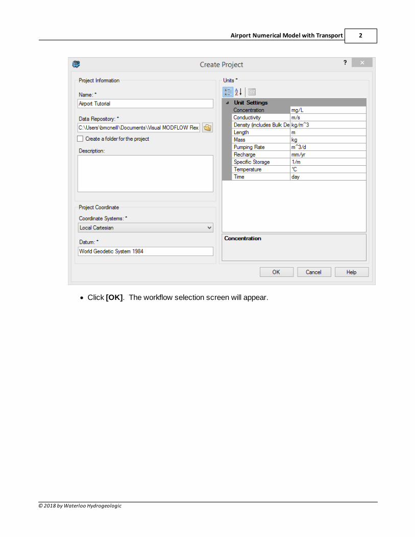
· Select [File] then [New Project..]. The Create Project dialog will appear.
· Type in project name 'Airport Tutorial'.
· Click the [ ] button, and navigate to a folder where you wish your projects to besaved, and click [OK].
· Define your coordinate system and datum (or just leave the Local Cartesian asdefaults).
· For this project, the default units will be fine.
The Create Project dialog should now look as follows:
Airport Numerical Model with Transport 2
© 2018 by Waterloo Hydrogeologic
· Click [OK]. The workflow selection screen will appear.
Visual MODFLOW Flex 5.13
© 2018 by Waterloo Hydrogeologic
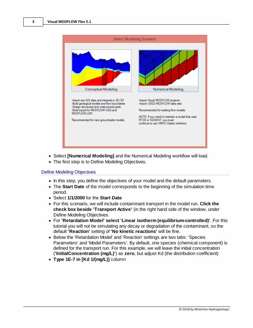
· Select [Numerical Modeling] and the Numerical Modeling workflow will load.
· The first step is to Define Modeling Objectives.
Define Modeling Objectives
· In this step, you define the objectives of your model and the default parameters.
· The Start Date of the model corresponds to the beginning of the simulation timeperiod.
· Select 1/1/2000 for the Start Date
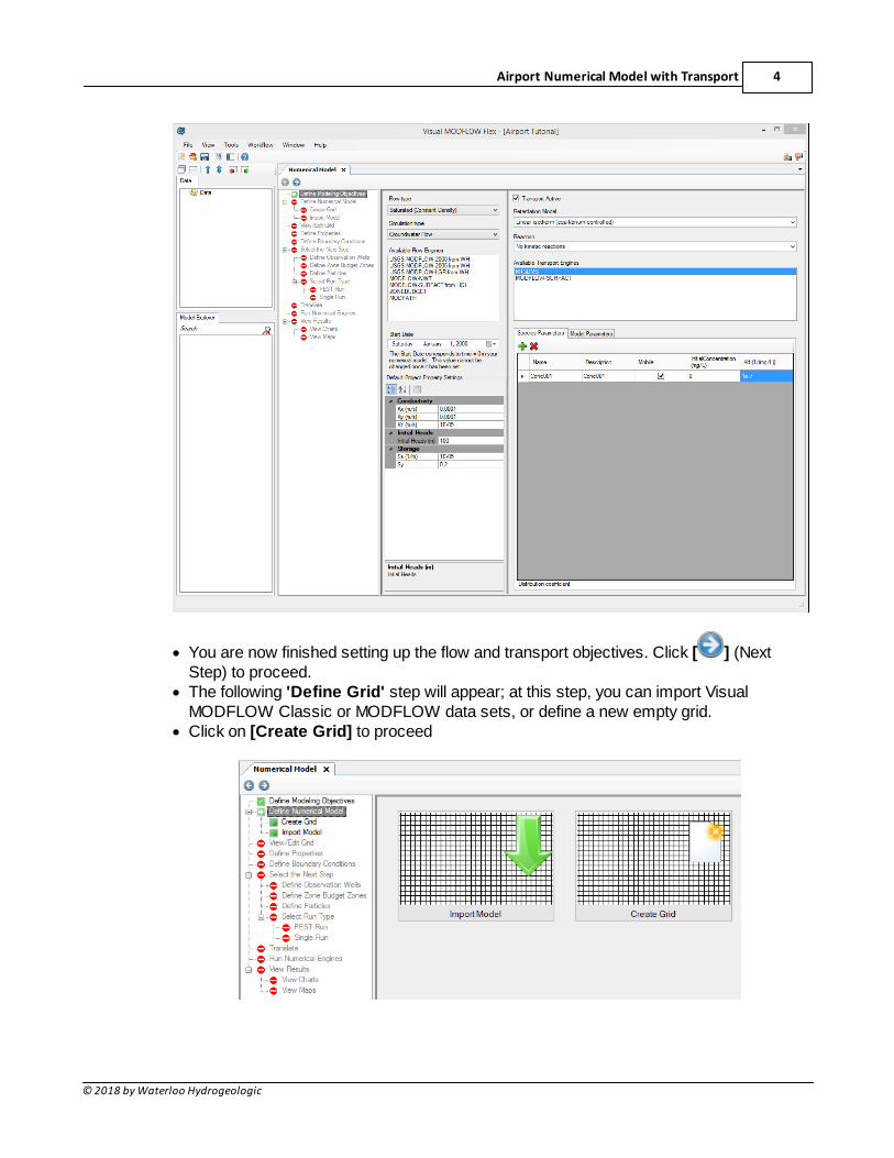
· For this scenario, we will include contaminant transport in the model run. Click thecheck box beside 'Transport Active' (in the right hand side of the window, underDefine Modeling Objectives.
· For 'Retardation Model' select 'Linear isotherm (equilibrium-controlled)'. For thistutorial you will not be simulating any decay or degradation of the contaminant, so thedefault 'Reaction' setting of 'No kinetic reactions' will be fine.
· Below the 'Retardation Model' and 'Reaction' settings are two tabs: 'SpeciesParameters' and 'Model Parameters'. By default, one species (chemical component) isdefined for the transport run. For this example, we will leave the initial concentration('InitialConcentration (mg/L)') as zero, but adjust Kd (the distribution coefficient)
· Type 1E-7 in [Kd 1/(mg/L)] column
Airport Numerical Model with Transport 4
© 2018 by Waterloo Hydrogeologic
· You are now finished setting up the flow and transport objectives. Click [ ] (NextStep) to proceed.
· The following 'Define Grid' step will appear; at this step, you can import VisualMODFLOW Classic or MODFLOW data sets, or define a new empty grid.
· Click on [Create Grid] to proceed
Visual MODFLOW Flex 5.15
© 2018 by Waterloo Hydrogeologic
Create Grid
· At this step, you can specify the dimensions of the Model Domain, and define thenumber of rows, columns, and layers for the finite difference grid. Type the followinginto the Grid Size section,
· Columns: 40
· Rows: 40
· For Grid Extents, enter 2000 for Xmax and 2000 for Ymax
· Under Define Vertical Grid, Type 3 for Number of Layers
Define Layer Elevations
· In Visual MODFLOW Flex, you can define the elevations of the tops and bottom of themodel layers. Or you can have varying layer elevations defined from Surface dataobjects. Surfaces could be from data objects you imported from Surfer (.GRD, ESRI.ASI, .DEM), or from Surfaces you have created through interpolating XYZ points. In thisexercise, you will import 4 surfaces (from Surfer .GRD files), then use these to definethe layer elevations.
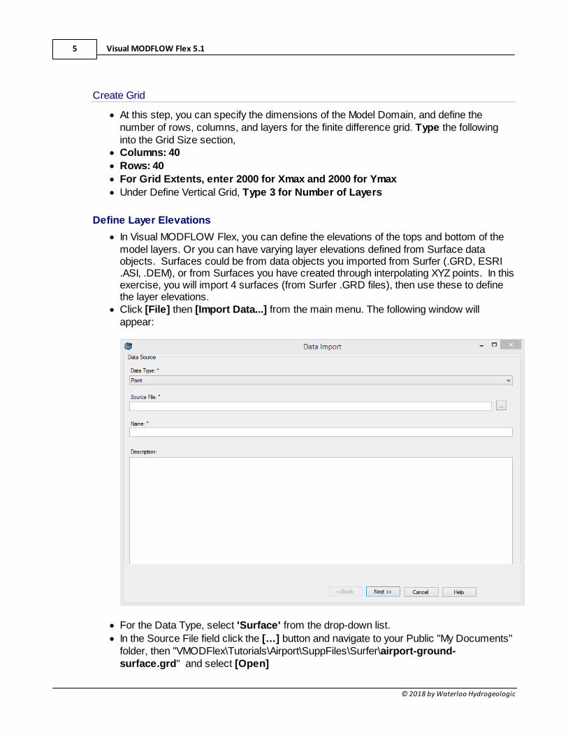
· Click [File] then [Import Data...] from the main menu. The following window willappear:
· For the Data Type, select 'Surface' from the drop-down list.
· In the Source File field click the […] button and navigate to your Public "My Documents"folder, then "VMODFlex\Tutorials\Airport\SuppFiles\Surfer\airport-ground-surface.grd" and select [Open]
Airport Numerical Model with Transport 6
© 2018 by Waterloo Hydrogeologic
· Click [Next>>]
· Click [Next>>] (accept the defaults)
· Click [Next>>] (accept the defaults)
· Click [Finish]. You should now see a new "airport-ground-surface" data object appearin the data tree, in the top left corner of the window.
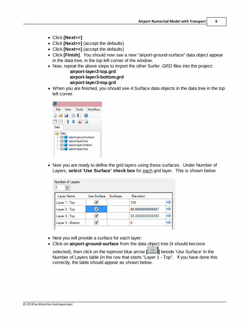
· Now, repeat the above steps to import the other Surfer .GRD files into the project: airport-layer2-top.grdairport-layer3-bottom.grdairport-layer3-top.grd
· When you are finished, you should see 4 Surface data objects in the data tree in the topleft corner.
· Now you are ready to define the grid layers using these surfaces. Under Number ofLayers, select 'Use Surface' check box for each grid layer. This is shown below
· Next you will provide a surface for each layer;
· Click on airport-ground-surface from the data object tree (it should become
selected), then click on the topmost blue arrow [ ] beside 'Use Surface' in theNumber of Layers table (in the row that starts "Layer 1 - Top". If you have done thiscorrectly, the table should appear as shown below.
Visual MODFLOW Flex 5.17
© 2018 by Waterloo Hydrogeologic
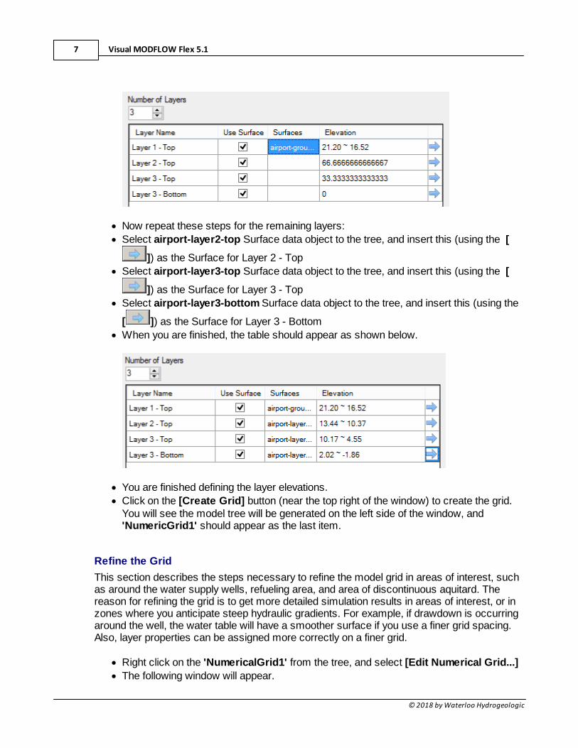
· Now repeat these steps for the remaining layers:
· Select airport-layer2-top Surface data object to the tree, and insert this (using the [
]) as the Surface for Layer 2 - Top
· Select airport-layer3-top Surface data object to the tree, and insert this (using the [
]) as the Surface for Layer 3 - Top
· Select airport-layer3-bottom Surface data object to the tree, and insert this (using the
[ ]) as the Surface for Layer 3 - Bottom
· When you are finished, the table should appear as shown below.
· You are finished defining the layer elevations.
· Click on the [Create Grid] button (near the top right of the window) to create the grid.You will see the model tree will be generated on the left side of the window, and'NumericGrid1' should appear as the last item.
Refine the Grid
This section describes the steps necessary to refine the model grid in areas of interest, suchas around the water supply wells, refueling area, and area of discontinuous aquitard. Thereason for refining the grid is to get more detailed simulation results in areas of interest, or inzones where you anticipate steep hydraulic gradients. For example, if drawdown is occurringaround the well, the water table will have a smoother surface if you use a finer grid spacing.Also, layer properties can be assigned more correctly on a finer grid.
· Right click on the 'NumericalGrid1' from the tree, and select [Edit Numerical Grid...]
· The following window will appear.
Airport Numerical Model with Transport 8
© 2018 by Waterloo Hydrogeologic
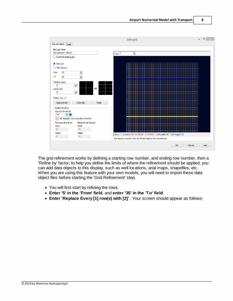
The grid refinement works by defining a starting row number, and ending row number, then a'Refine by' factor; to help you define the limits of where the refinement should be applied, youcan add data objects to this display, such as well locations, arial maps, shapefiles, etc. When you are using this feature with your own models, you will need to import these dataobject files before starting the 'Grid Refinement' step.
· You will first start by refining the rows.
· Enter '5' in the 'From' field, and enter '35' in the 'To' field.
· Enter 'Replace Every [1] row(s) with [2]'. Your screen should appear as follows:
Visual MODFLOW Flex 5.19
© 2018 by Waterloo Hydrogeologic
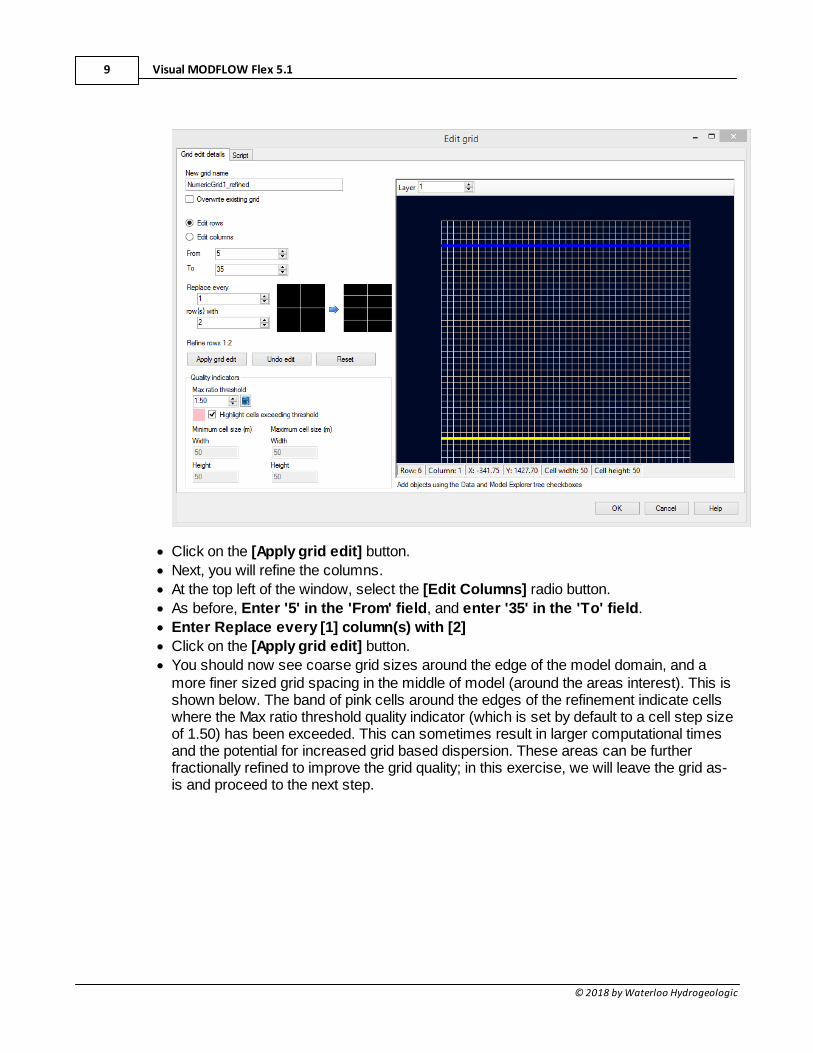
· Click on the [Apply grid edit] button.
· Next, you will refine the columns.
· At the top left of the window, select the [Edit Columns] radio button.
· As before, Enter '5' in the 'From' field, and enter '35' in the 'To' field.
· Enter Replace every [1] column(s) with [2]
· Click on the [Apply grid edit] button.
· You should now see coarse grid sizes around the edge of the model domain, and amore finer sized grid spacing in the middle of model (around the areas interest). This isshown below. The band of pink cells around the edges of the refinement indicate cellswhere the Max ratio threshold quality indicator (which is set by default to a cell step sizeof 1.50) has been exceeded. This can sometimes result in larger computational timesand the potential for increased grid based dispersion. These areas can be furtherfractionally refined to improve the grid quality; in this exercise, we will leave the grid as-is and proceed to the next step.

Airport Numerical Model with Transport 10
© 2018 by Waterloo Hydrogeologic
· Click on the [OK] button.
· In the Model Explorer tree, right click on 'NumericGrid1_refined' and click [Convertto Numerical Model]. This opens a new workflow for the refined grid and adds a 'Run'node with related child nodes in the Model Explorer for the new refined grid. This willgenerate the model run folder in the Model tree, which includes input and outputdirectories, and default flow and transport properties.
· Now is a good time to save the project. Click [File] then [Save Project] from the mainmenu.
· In the next section, you will view the numerical grid that you just created.
· Click on the Define Properties step or click the next button [ ] to proceed.
Define Flow Properties
This section will guide you through the steps necessary to design a model with layers ofhighly contrasting hydraulic conductivities.
· First, ensure that 'Conductivity' is selected in the first dropdown menu under the'Toolbox'
· Click on the [Edit...] button and Type the following values in the top row of the window:o Kx (m/s): 2E-4, then use [F2] to propagate through all cellso Ky (m/s): 2E-4, then use [F2] to propagate through all cellso Kz (m/s): 2E-4, then use [F2] to propagate through all cells
· Click [OK] to accept these values.
Visual MODFLOW Flex 5.111
© 2018 by Waterloo Hydrogeologic
Note: it may take a moment for Flex to process this change.
In this case the Kx, Ky, and Kz values are the same, indicating the assigned property valuesare assumed horizontally and vertically isotropic. However, anisotropic property values can beassigned to a model by modifying the Conductivity Database
In this three layer model, layer 1 represents the upper aquifer, and layer 3 represents thelower aquifer. Layer 2 represents the aquitard separating the upper and lower aquifers. Forthis example, we will use the previously assigned hydraulic conductivity values (Zone# 1) formodel layers 1 and 3 (representing the aquifers) and assign different Conductivity values (i.e.a new Zone) for model layer 2 (representing the aquitard). Note that layer 1 is the top modellayer.
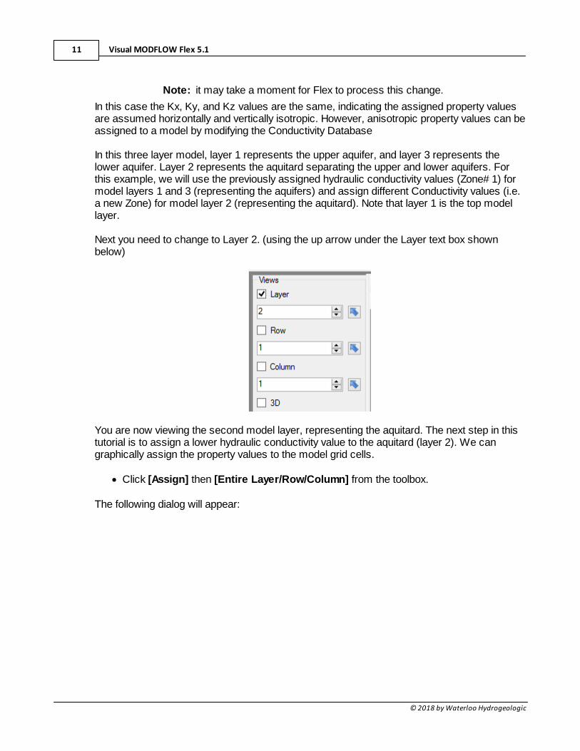
Next you need to change to Layer 2. (using the up arrow under the Layer text box shownbelow)
You are now viewing the second model layer, representing the aquitard. The next step in thistutorial is to assign a lower hydraulic conductivity value to the aquitard (layer 2). We cangraphically assign the property values to the model grid cells.
· Click [Assign] then [Entire Layer/Row/Column] from the toolbox.
The following dialog will appear:
Airport Numerical Model with Transport 12
© 2018 by Waterloo Hydrogeologic
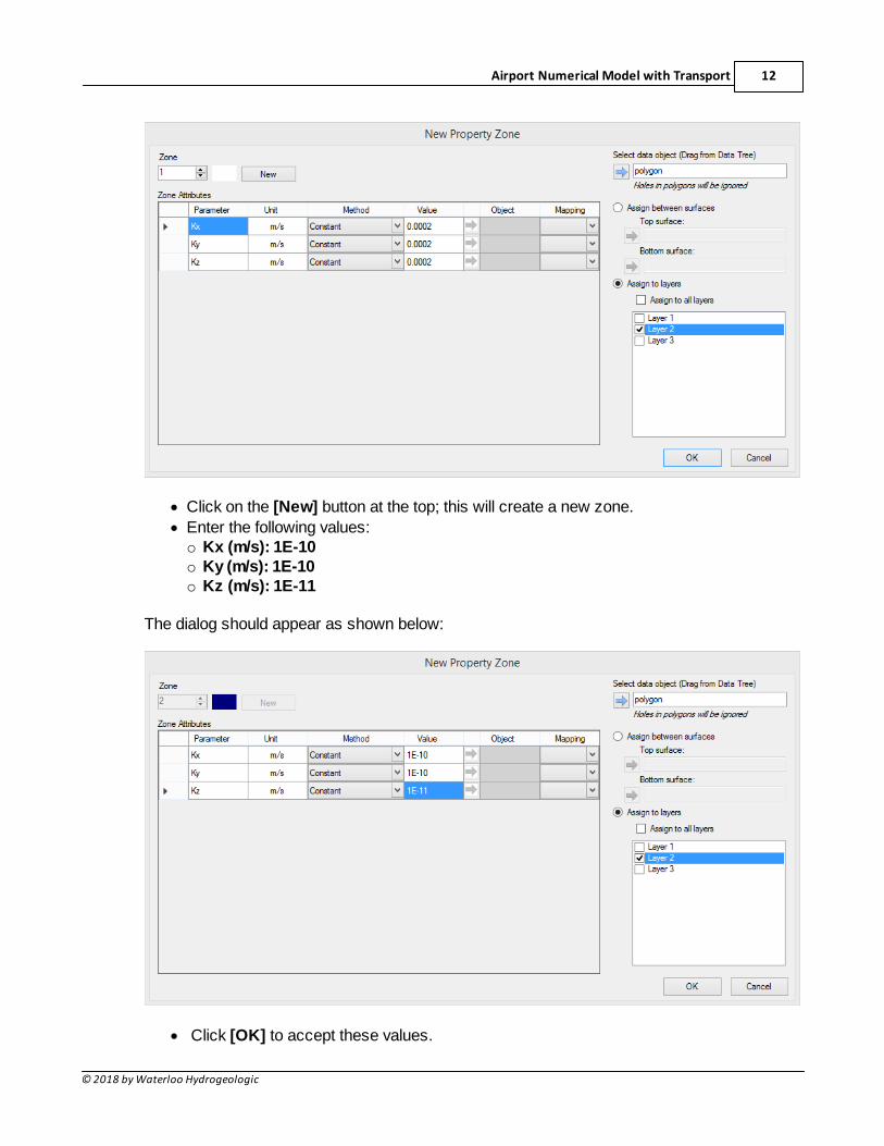
· Click on the [New] button at the top; this will create a new zone.
· Enter the following values:o Kx (m/s): 1E-10o Ky (m/s): 1E-10o Kz (m/s): 1E-11
The dialog should appear as shown below:
· Click [OK] to accept these values.
Visual MODFLOW Flex 5.113
© 2018 by Waterloo Hydrogeologic
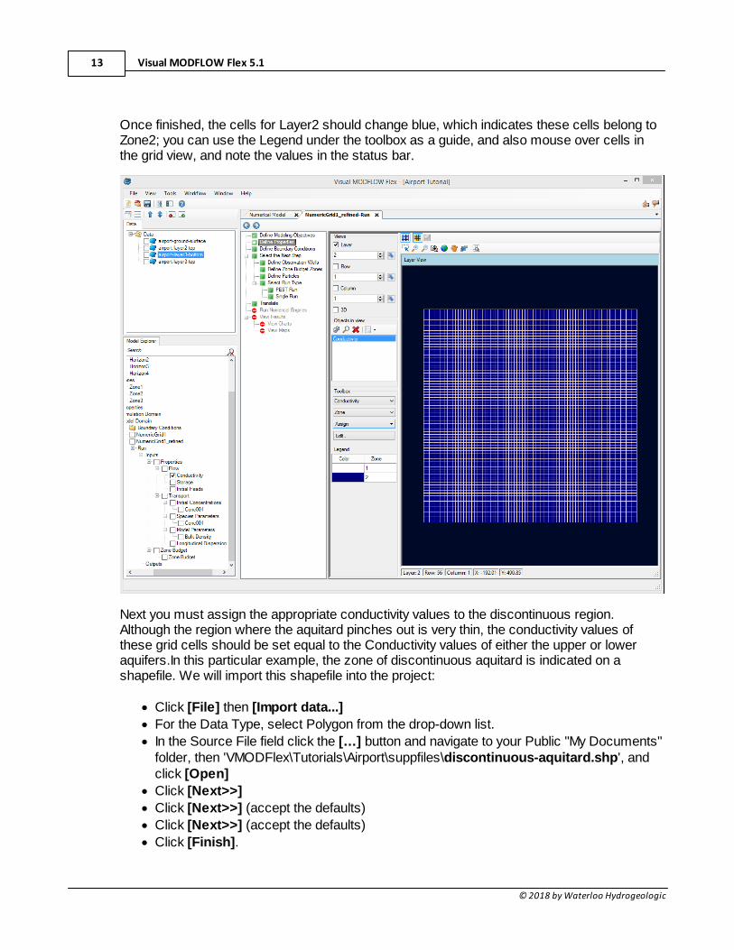
Once finished, the cells for Layer2 should change blue, which indicates these cells belong toZone2; you can use the Legend under the toolbox as a guide, and also mouse over cells inthe grid view, and note the values in the status bar.
Next you must assign the appropriate conductivity values to the discontinuous region.Although the region where the aquitard pinches out is very thin, the conductivity values ofthese grid cells should be set equal to the Conductivity values of either the upper or loweraquifers.In this particular example, the zone of discontinuous aquitard is indicated on ashapefile. We will import this shapefile into the project:
· Click [File] then [Import data...]
· For the Data Type, select Polygon from the drop-down list.
· In the Source File field click the […] button and navigate to your Public "My Documents"folder, then 'VMODFlex\Tutorials\Airport\suppfiles\discontinuous-aquitard.shp', andclick [Open]
· Click [Next>>]
· Click [Next>>] (accept the defaults)
· Click [Next>>] (accept the defaults)
· Click [Finish].
Airport Numerical Model with Transport 14
© 2018 by Waterloo Hydrogeologic
· You should now see a new data object, 'discontinuous-aquitard' appear in the datatree, in the top left corner of the window.
· Click on the box beside this data object in the tree .
· The data object should now appear in the Layer View of the grid.
· Zoom into this area (using the mouse wheel, or the Zoom in button on the toolbar).
· Click [Assign] then [Using Data Object] from the toolbox.
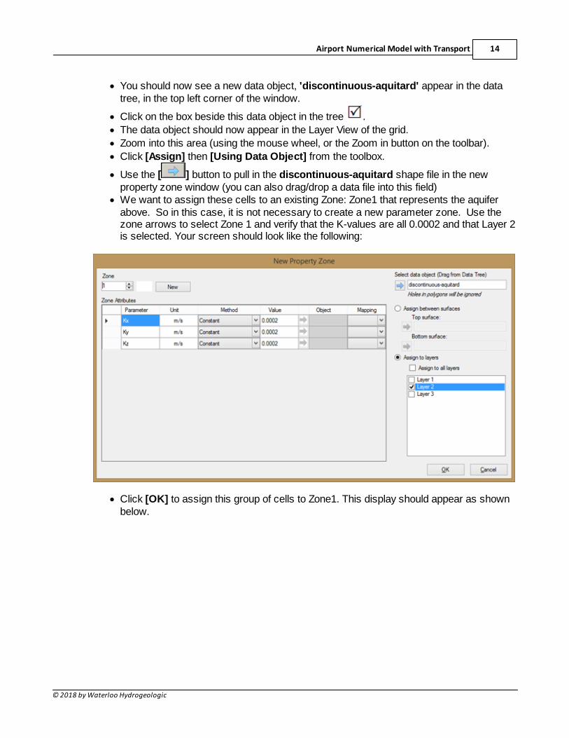
· Use the [ ] button to pull in the discontinuous-aquitard shape file in the newproperty zone window (you can also drag/drop a data file into this field)
· We want to assign these cells to an existing Zone: Zone1 that represents the aquiferabove. So in this case, it is not necessary to create a new parameter zone. Use thezone arrows to select Zone 1 and verify that the K-values are all 0.0002 and that Layer 2is selected. Your screen should look like the following:
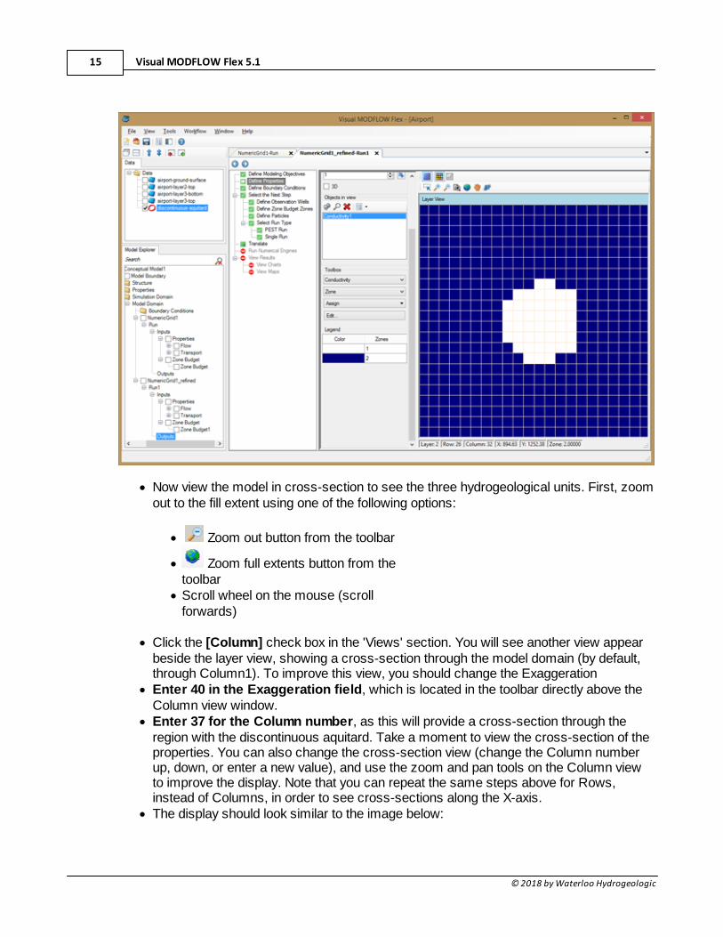
· Click [OK] to assign this group of cells to Zone1. This display should appear as shownbelow.
Visual MODFLOW Flex 5.115
© 2018 by Waterloo Hydrogeologic
· Now view the model in cross-section to see the three hydrogeological units. First, zoomout to the fill extent using one of the following options:
· Zoom out button from the toolbar
· Zoom full extents button from thetoolbar
· Scroll wheel on the mouse (scrollforwards)
· Click the [Column] check box in the 'Views' section. You will see another view appearbeside the layer view, showing a cross-section through the model domain (by default,through Column1). To improve this view, you should change the Exaggeration
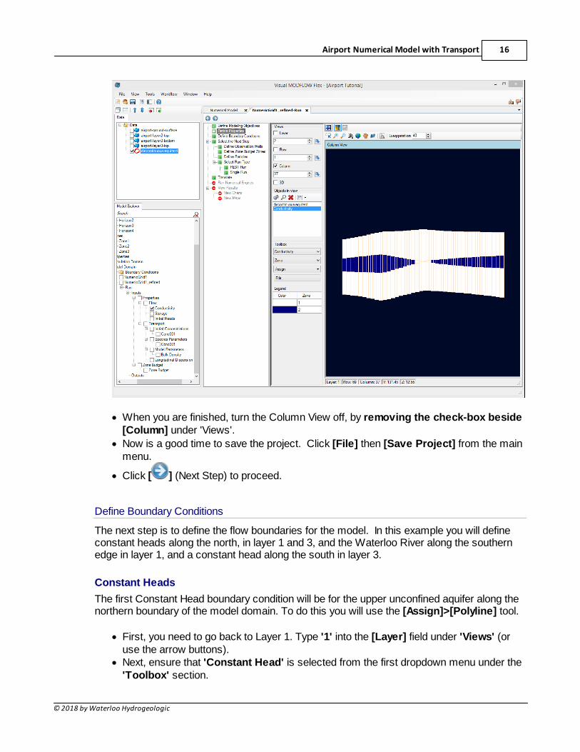
· Enter 40 in the Exaggeration field, which is located in the toolbar directly above theColumn view window.
· Enter 37 for the Column number, as this will provide a cross-section through theregion with the discontinuous aquitard. Take a moment to view the cross-section of theproperties. You can also change the cross-section view (change the Column numberup, down, or enter a new value), and use the zoom and pan tools on the Column viewto improve the display. Note that you can repeat the same steps above for Rows,instead of Columns, in order to see cross-sections along the X-axis.
· The display should look similar to the image below:
Airport Numerical Model with Transport 16
© 2018 by Waterloo Hydrogeologic
· When you are finished, turn the Column View off, by removing the check-box beside[Column] under 'Views'.
· Now is a good time to save the project. Click [File] then [Save Project] from the mainmenu.
· Click [ ] (Next Step) to proceed.
Define Boundary Conditions
The next step is to define the flow boundaries for the model. In this example you will defineconstant heads along the north, in layer 1 and 3, and the Waterloo River along the southernedge in layer 1, and a constant head along the south in layer 3.
Constant Heads
The first Constant Head boundary condition will be for the upper unconfined aquifer along thenorthern boundary of the model domain. To do this you will use the [Assign]>[Polyline] tool.
· First, you need to go back to Layer 1. Type '1' into the [Layer] field under 'Views' (oruse the arrow buttons).
· Next, ensure that 'Constant Head' is selected from the first dropdown menu under the'Toolbox' section.
Visual MODFLOW Flex 5.117
© 2018 by Waterloo Hydrogeologic
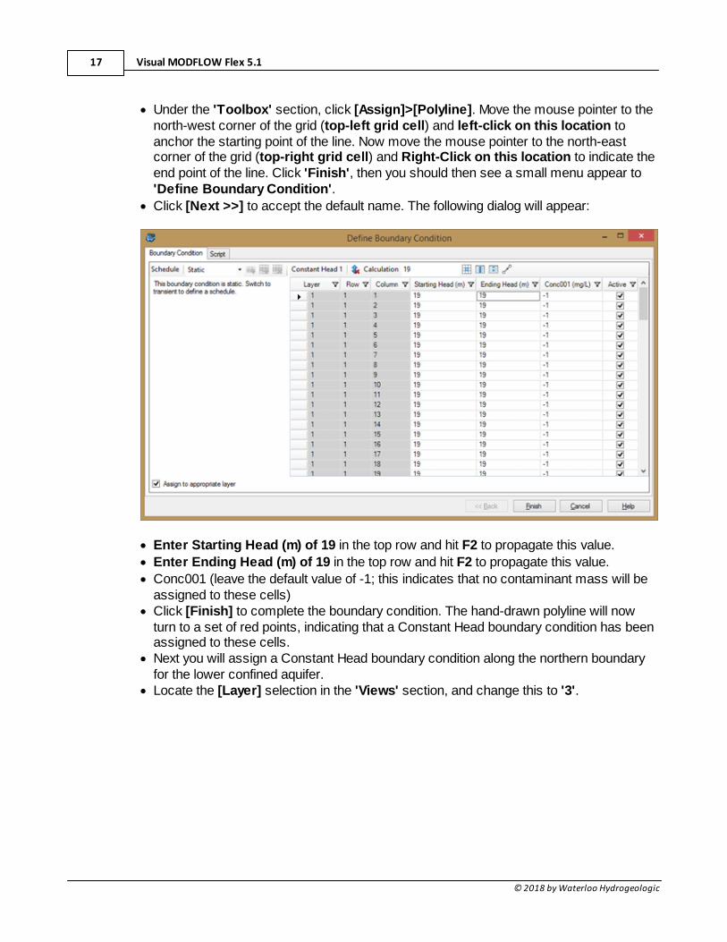
· Under the 'Toolbox' section, click [Assign]>[Polyline]. Move the mouse pointer to thenorth-west corner of the grid (top-left grid cell) and left-click on this location toanchor the starting point of the line. Now move the mouse pointer to the north-eastcorner of the grid (top-right grid cell) and Right-Click on this location to indicate theend point of the line. Click 'Finish', then you should then see a small menu appear to'Define Boundary Condition'.
· Click [Next >>] to accept the default name. The following dialog will appear:
· Enter Starting Head (m) of 19 in the top row and hit F2 to propagate this value.
· Enter Ending Head (m) of 19 in the top row and hit F2 to propagate this value.
· Conc001 (leave the default value of -1; this indicates that no contaminant mass will beassigned to these cells)
· Click [Finish] to complete the boundary condition. The hand-drawn polyline will nowturn to a set of red points, indicating that a Constant Head boundary condition has beenassigned to these cells.
· Next you will assign a Constant Head boundary condition along the northern boundaryfor the lower confined aquifer.
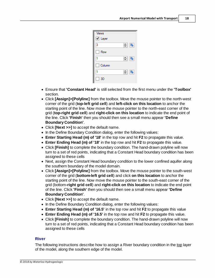
· Locate the [Layer] selection in the 'Views' section, and change this to '3'.
Airport Numerical Model with Transport 18
© 2018 by Waterloo Hydrogeologic
· Ensure that 'Constant Head' is still selected from the first menu under the 'Toolbox'section.
· Click [Assign]>[Polyline] from the toolbox. Move the mouse pointer to the north-westcorner of the grid (top-left grid cell) and left-click on this location to anchor thestarting point of the line. Now move the mouse pointer to the north-east corner of thegrid (top-right grid cell) and right-click on this location to indicate the end point ofthe line. Click 'Finish' then you should then see a small menu appear 'DefineBoundary Condition'.
· Click [Next >>] to accept the default name.
· In the Define Boundary Condition dialog, enter the following values:
· Enter Starting Head (m) of '18' in the top row and hit F2 to propagate this value.
· Enter Ending Head (m) of '18' in the top row and hit F2 to propagate this value.
· Click [Finish] to complete the boundary condition. The hand-drawn polyline will nowturn to a set of red points, indicating that a Constant Head boundary condition has beenassigned to these cells
· Next, assign the Constant Head boundary condition to the lower confined aquifer alongthe southern boundary of the model domain.
· Click [Assign]>[Polyline] from the toolbox. Move the mouse pointer to the south-westcorner of the grid (bottom-left grid cell) and click on this location to anchor thestarting point of the line. Now move the mouse pointer to the south-east corner of thegrid (bottom-right grid cell) and right-click on this location to indicate the end pointof the line. Click 'Finish' then you should then see a small menu appear 'DefineBoundary Condition'.
· Click [Next >>] to accept the default name.
· In the Define Boundary Condition dialog, enter the following values:
· Enter Starting Head (m) of '16.5' in the top row and hit F2 to propagate this value
· Enter Ending Head (m) of '16.5' in the top row and hit F2 to propagate this value.
· Click [Finish] to complete the boundary condition. The hand-drawn polyline will nowturn to a set of red points, indicating that a Constant Head boundary condition has beenassigned to these cells
River
The following instructions describe how to assign a River boundary condition in the top layerof the model, along the southern edge of the model.
Visual MODFLOW Flex 5.119
© 2018 by Waterloo Hydrogeologic
· First, you need to go back to Layer 1 (using the steps explained previously)
· Now we need to import our river data object (using the steps explained previously;[File]>[Import Data]>'Polyline'>'river.shp')
· Select 'River' from the first dropdown menu in the 'Toolbox' section.
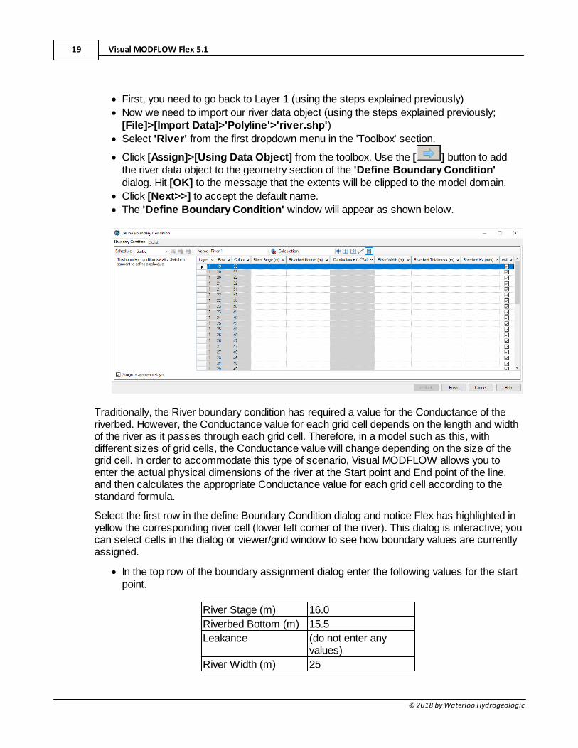
· Click [Assign]>[Using Data Object] from the toolbox. Use the [ ] button to addthe river data object to the geometry section of the 'Define Boundary Condition'dialog. Hit [OK] to the message that the extents will be clipped to the model domain.
· Click [Next>>] to accept the default name.
· The 'Define Boundary Condition' window will appear as shown below.
Traditionally, the River boundary condition has required a value for the Conductance of theriverbed. However, the Conductance value for each grid cell depends on the length and widthof the river as it passes through each grid cell. Therefore, in a model such as this, withdifferent sizes of grid cells, the Conductance value will change depending on the size of thegrid cell. In order to accommodate this type of scenario, Visual MODFLOW allows you toenter the actual physical dimensions of the river at the Start point and End point of the line,and then calculates the appropriate Conductance value for each grid cell according to thestandard formula.
Select the first row in the define Boundary Condition dialog and notice Flex has highlighted inyellow the corresponding river cell (lower left corner of the river). This dialog is interactive; youcan select cells in the dialog or viewer/grid window to see how boundary values are currentlyassigned.
· In the top row of the boundary assignment dialog enter the following values for the startpoint.
River Stage (m) 16.0
Riverbed Bottom (m) 15.5
Leakance (do not enter anyvalues)
River Width (m) 25
Airport Numerical Model with Transport 20
© 2018 by Waterloo Hydrogeologic
Riverbed Thickness(m)
0.1
Riverbed Kz (m/s) 1E-4
Leakance from the river will be calculated based on the parameters you define. Formore details on the calculation, refer to Boundary Conditions Theory
· Now you will define the values for the End Point of the river.
· Scroll to the bottom row in the Define Boundary Condition dialog and click in it. Noticethe river end cell is now highlighted yellow in the grid view.
· Now define the values at this end point, in the parameters grid, based on the valuesbelow:
River Stage (m) 15.5
Riverbed Bottom (m) 15.0
Conductance (m2/d) (do not enter anyvalues)
River Width (m) 25
Riverbed Thickness(m)
0.1
Riverbed Conductivity(m/s)
1E-4
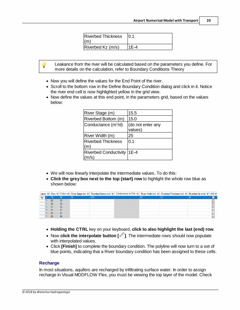
· We will now linearly interpolate the intermediate values. To do this:
· Click the grey box next to the top (start) row to highlight the whole row blue asshown below:
· Holding the CTRL key on your keyboard, click to also highlight the last (end) row.
· Now click the interpolate button [ ]. The intermediate rows should now populatewith interpolated values.
· Click [Finish] to complete the boundary condition. The polyline will now turn to a set ofblue points, indicating that a River boundary condition has been assigned to these cells.
Recharge
In most situations, aquifers are recharged by infiltrating surface water. In order to assignrecharge in Visual MODFLOW Flex, you must be viewing the top layer of the model. Check
Visual MODFLOW Flex 5.121
© 2018 by Waterloo Hydrogeologic
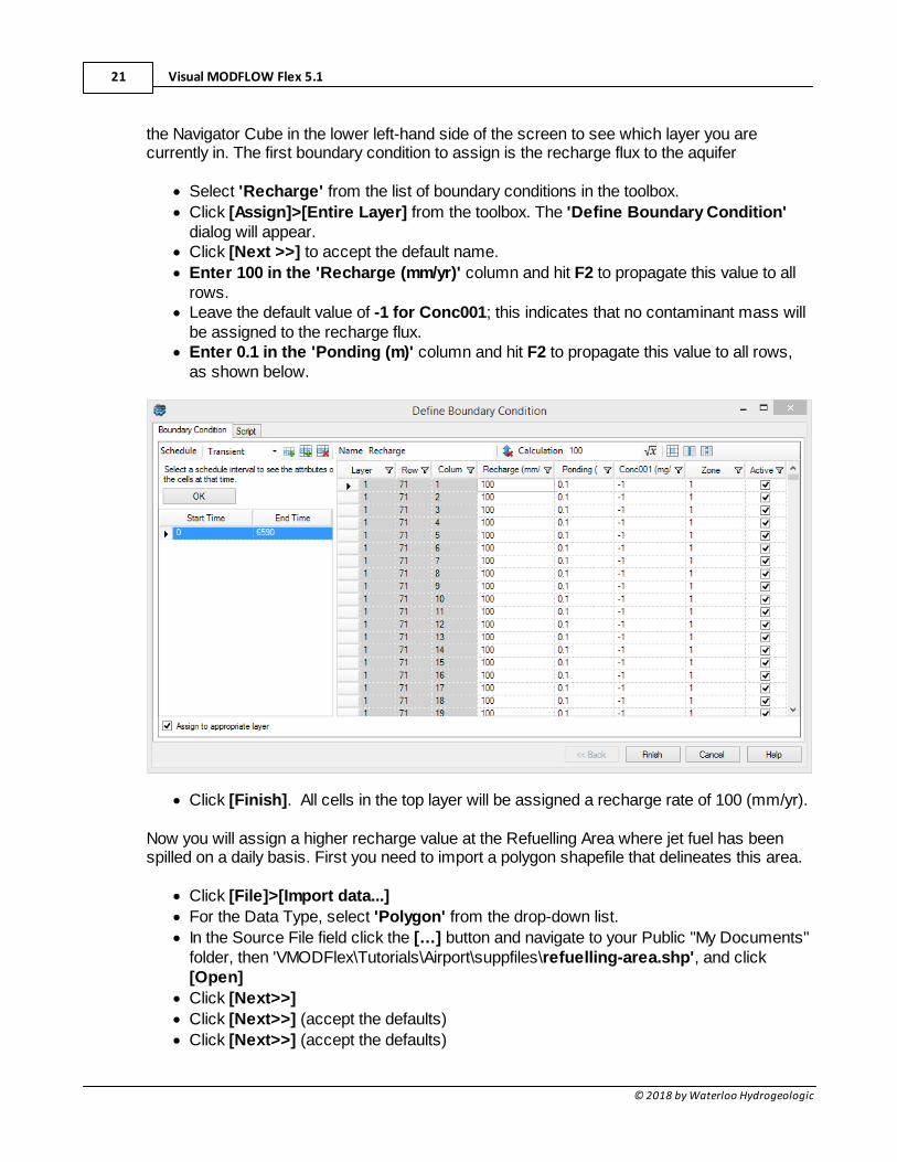
the Navigator Cube in the lower left-hand side of the screen to see which layer you arecurrently in. The first boundary condition to assign is the recharge flux to the aquifer
· Select 'Recharge' from the list of boundary conditions in the toolbox.
· Click [Assign]>[Entire Layer] from the toolbox. The 'Define Boundary Condition'dialog will appear.
· Click [Next >>] to accept the default name.
· Enter 100 in the 'Recharge (mm/yr)' column and hit F2 to propagate this value to allrows.
· Leave the default value of -1 for Conc001; this indicates that no contaminant mass willbe assigned to the recharge flux.
· Enter 0.1 in the 'Ponding (m)' column and hit F2 to propagate this value to all rows,as shown below.
· Click [Finish]. All cells in the top layer will be assigned a recharge rate of 100 (mm/yr).
Now you will assign a higher recharge value at the Refuelling Area where jet fuel has beenspilled on a daily basis. First you need to import a polygon shapefile that delineates this area.
· Click [File]>[Import data...]
· For the Data Type, select 'Polygon' from the drop-down list.
· In the Source File field click the […] button and navigate to your Public "My Documents"folder, then 'VMODFlex\Tutorials\Airport\suppfiles\refuelling-area.shp', and click[Open]
· Click [Next>>]
· Click [Next>>] (accept the defaults)
· Click [Next>>] (accept the defaults)
Airport Numerical Model with Transport 22
© 2018 by Waterloo Hydrogeologic
· Click [Finish]. You should now see a new data object, 'refuelling-area' appear in thedata tree, in the top left corner of the window.
· Click on the box beside this data object in the tree . The data object should nowappear in the Layer View of the grid (it is located in the top middle of the site).
Note: you may need to uncheck 'Recharge' from the Model Explorer tree tomake the view less cluttered.
· Zoom into this area (using the mouse wheel, or the Zoom in button on the toolbar).
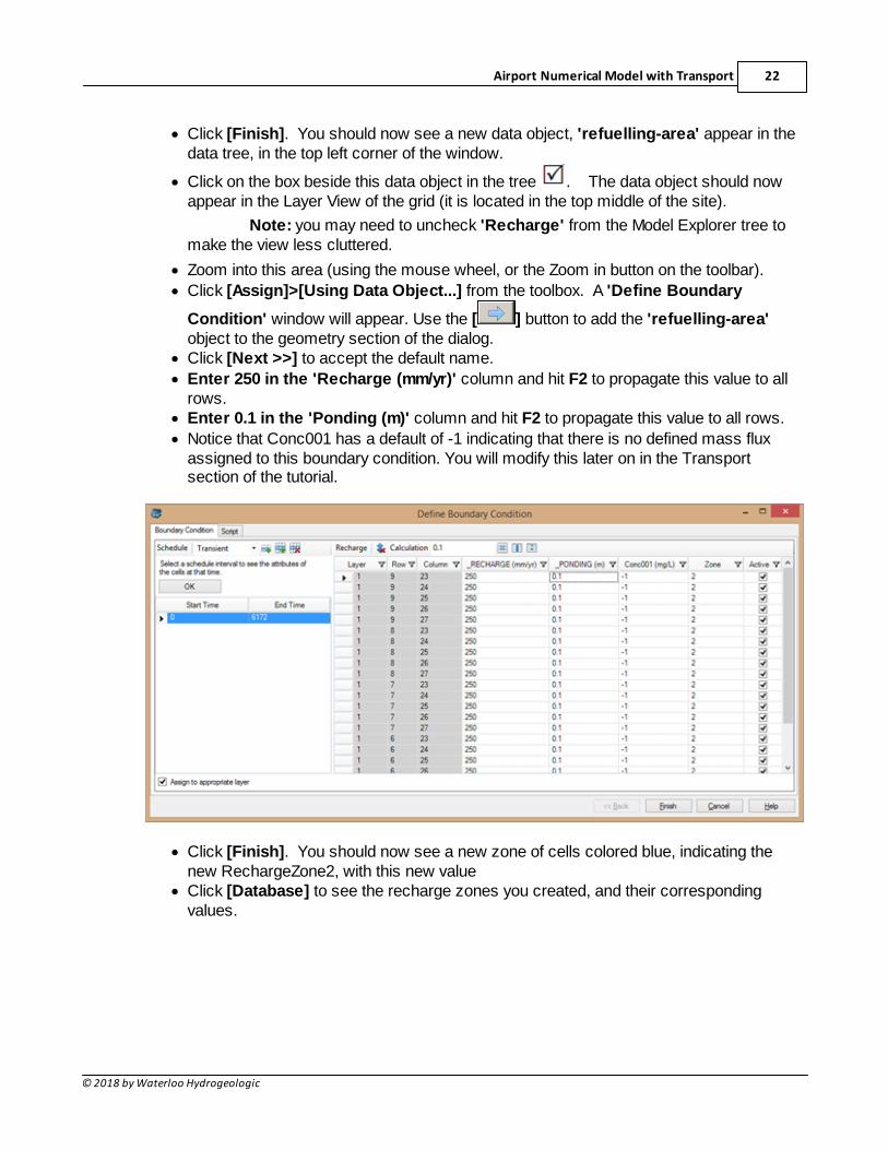
· Click [Assign]>[Using Data Object...] from the toolbox. A 'Define Boundary
Condition' window will appear. Use the [ ] button to add the 'refuelling-area'object to the geometry section of the dialog.
· Click [Next >>] to accept the default name.
· Enter 250 in the 'Recharge (mm/yr)' column and hit F2 to propagate this value to allrows.
· Enter 0.1 in the 'Ponding (m)' column and hit F2 to propagate this value to all rows.
· Notice that Conc001 has a default of -1 indicating that there is no defined mass fluxassigned to this boundary condition. You will modify this later on in the Transportsection of the tutorial.
· Click [Finish]. You should now see a new zone of cells colored blue, indicating thenew RechargeZone2, with this new value
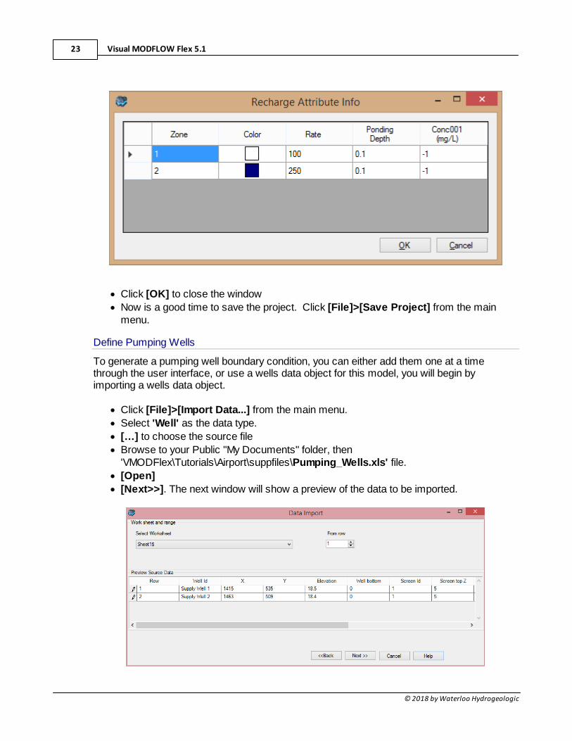
· Click [Database] to see the recharge zones you created, and their correspondingvalues.
Visual MODFLOW Flex 5.123
© 2018 by Waterloo Hydrogeologic
· Click [OK] to close the window
· Now is a good time to save the project. Click [File]>[Save Project] from the mainmenu.
Define Pumping Wells
To generate a pumping well boundary condition, you can either add them one at a timethrough the user interface, or use a wells data object for this model, you will begin byimporting a wells data object.
· Click [File]>[Import Data...] from the main menu.
· Select 'Well' as the data type.
· […] to choose the source file
· Browse to your Public "My Documents" folder, then'VMODFlex\Tutorials\Airport\suppfiles\Pumping_Wells.xls' file.
· [Open]
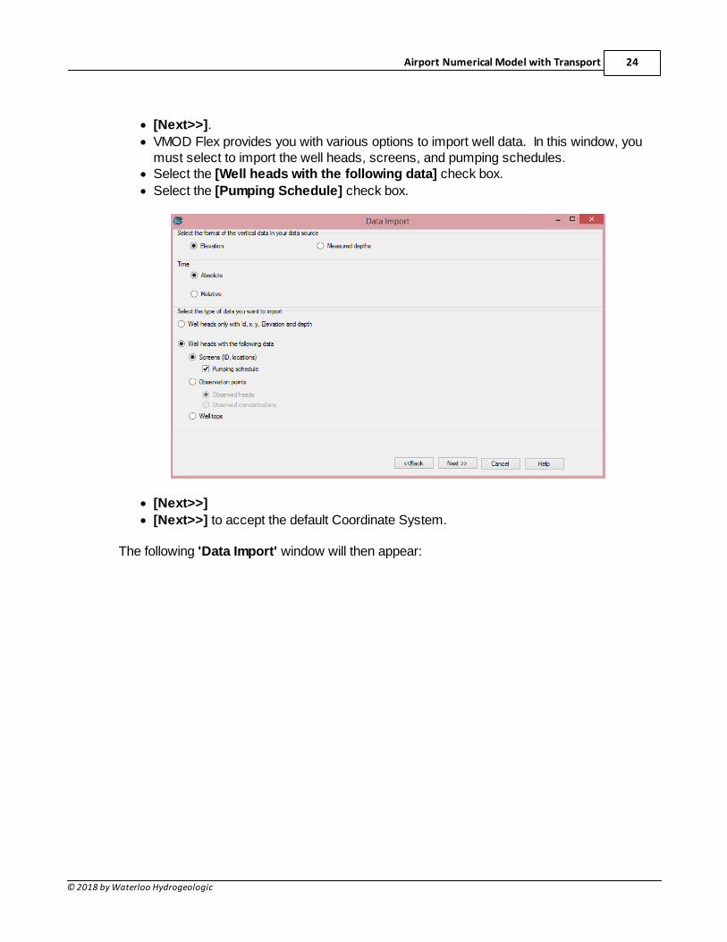
· [Next>>]. The next window will show a preview of the data to be imported.
Airport Numerical Model with Transport 24
© 2018 by Waterloo Hydrogeologic
· [Next>>].
· VMOD Flex provides you with various options to import well data. In this window, youmust select to import the well heads, screens, and pumping schedules.
· Select the [Well heads with the following data] check box.
· Select the [Pumping Schedule] check box.
· [Next>>]
· [Next>>] to accept the default Coordinate System.
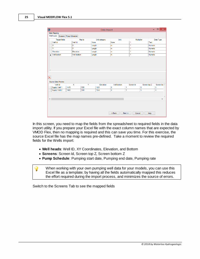
The following 'Data Import' window will then appear:
Visual MODFLOW Flex 5.125
© 2018 by Waterloo Hydrogeologic
In this screen, you need to map the fields from the spreadsheet to required fields in the dataimport utility. If you prepare your Excel file with the exact column names that are expected byVMOD Flex, then no mapping is required and this can save you time. For this exercise, thesource Excel file has the map names pre-defined. Take a moment to review the requiredfields for the Wells import:
· Well heads: Well ID, XY Coordinates, Elevation, and Bottom
· Screens: Screen Id, Screen top Z, Screen bottom Z
· Pump Schedule: Pumping start date, Pumping end date, Pumping rate
When working with your own pumping well data for your models, you can use thisExcel file as a template; by having all the fields automatically mapped this reducesthe effort required during the import process, and minimizes the source of errors.
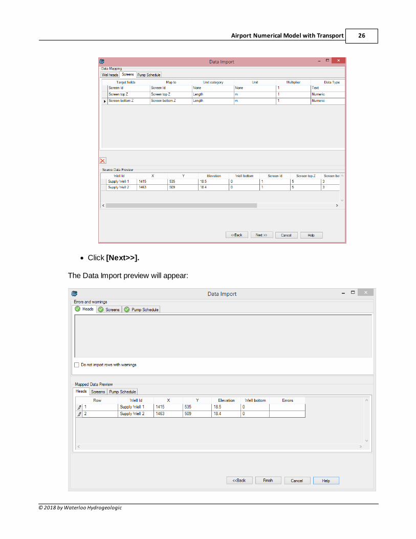
Switch to the Screens Tab to see the mapped fields
Airport Numerical Model with Transport 26
© 2018 by Waterloo Hydrogeologic
· Click [Next>>].
The Data Import preview will appear:
Visual MODFLOW Flex 5.127
© 2018 by Waterloo Hydrogeologic
· You should see a series of green check marks next to the 'Heads', 'Screens' and'Pump Schedule' tabs indicating that there were no import errors.
· Click [Next>>].
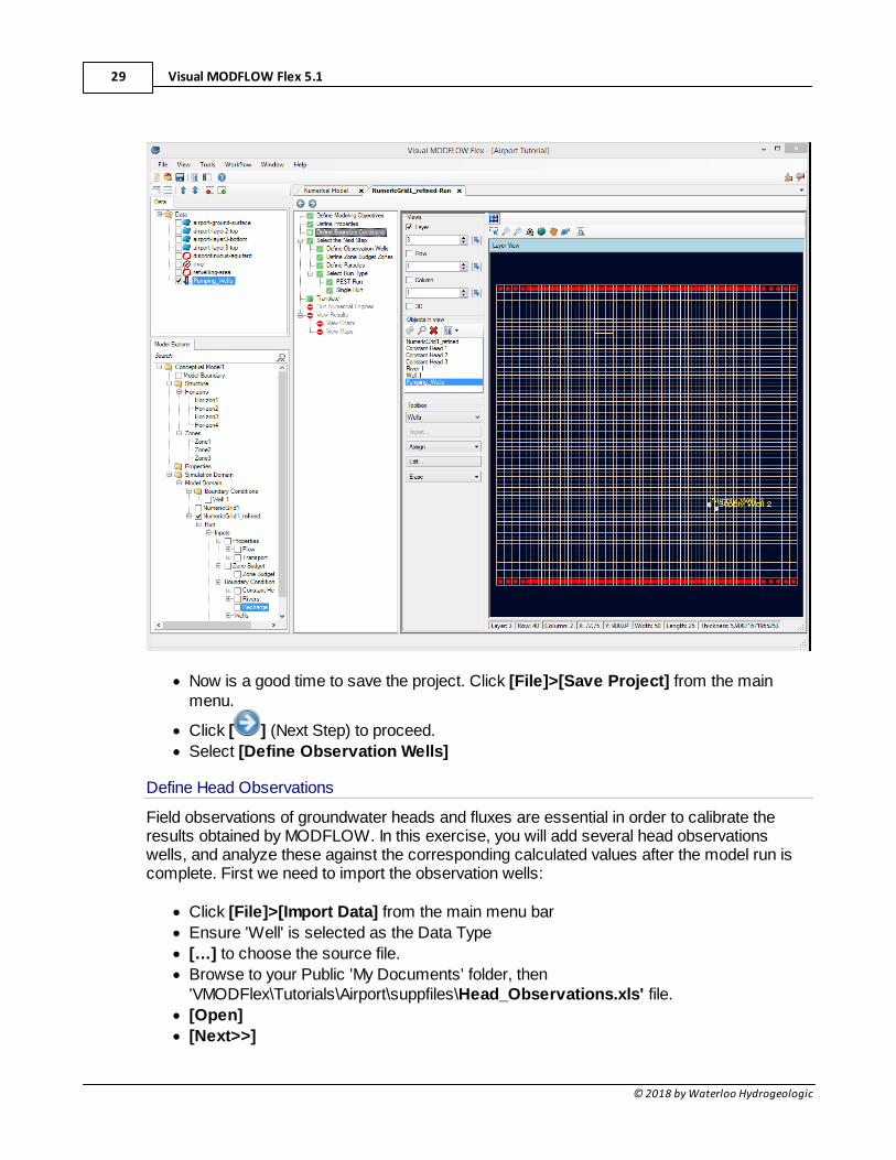
The 'Pumping_Wells' will now appear as a new data object in the Data tree.
Next, you need to add these wells to the Numerical Model
· At the Define Boundary Conditions step in the workflow, under Toolbox, choose 'Wells'from the first dropdown menu listing available boundary condition types.
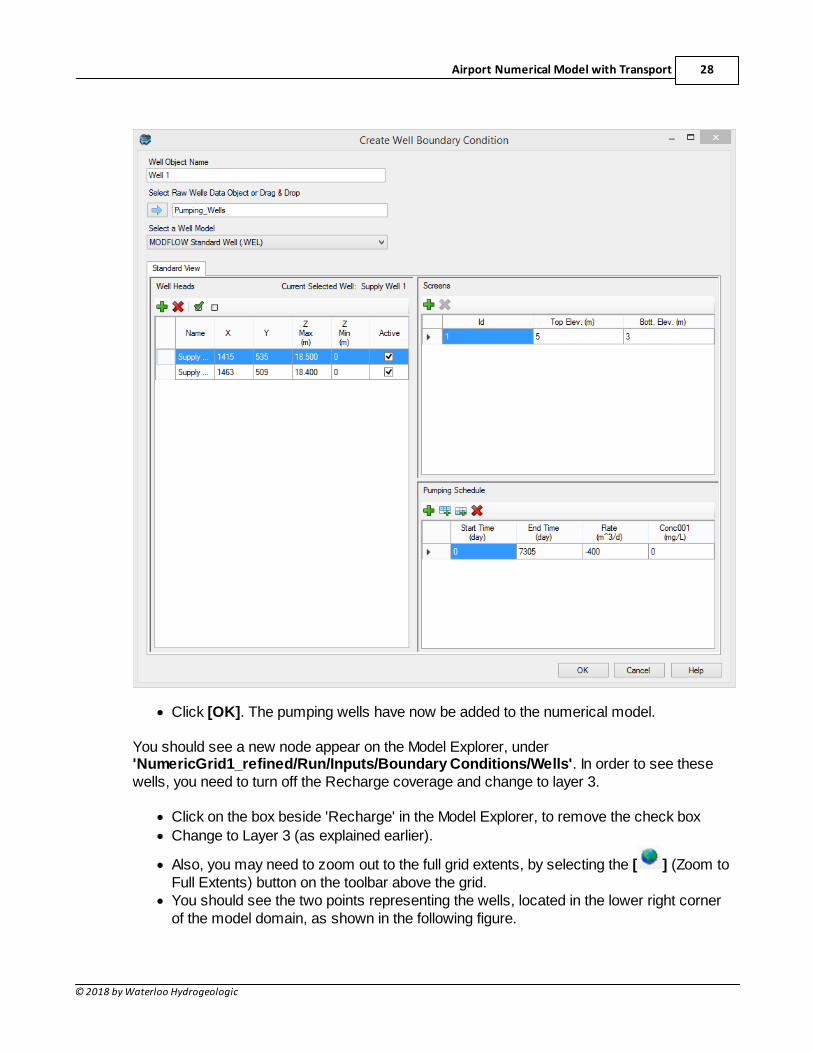
· Click the [Assign]>[Using Data Object] button. A 'Create Well Boundary Condition'window will appear.
· Select (highlight) the 'Pumping_Wells' data object from the Data Tree (you may needto move the Pumping Wells Boundary Condition dialog to the right in order to see this).
· Click [ ] button located in the middle of the 'Create Well Boundary Condition'window, under 'Select Raw Wells Data Object or Drag & Drop'. Once completed, yourdisplay should appear as shown below.
Airport Numerical Model with Transport 28
© 2018 by Waterloo Hydrogeologic
· Click [OK]. The pumping wells have now be added to the numerical model.
You should see a new node appear on the Model Explorer, under'NumericGrid1_refined/Run/Inputs/Boundary Conditions/Wells'. In order to see thesewells, you need to turn off the Recharge coverage and change to layer 3.
· Click on the box beside 'Recharge' in the Model Explorer, to remove the check box
· Change to Layer 3 (as explained earlier).
· Also, you may need to zoom out to the full grid extents, by selecting the [ ] (Zoom toFull Extents) button on the toolbar above the grid.
· You should see the two points representing the wells, located in the lower right cornerof the model domain, as shown in the following figure.
Visual MODFLOW Flex 5.129
© 2018 by Waterloo Hydrogeologic
· Now is a good time to save the project. Click [File]>[Save Project] from the mainmenu.
· Click [ ] (Next Step) to proceed.
· Select [Define Observation Wells]
Define Head Observations
Field observations of groundwater heads and fluxes are essential in order to calibrate theresults obtained by MODFLOW. In this exercise, you will add several head observationswells, and analyze these against the corresponding calculated values after the model run iscomplete. First we need to import the observation wells:
· Click [File]>[Import Data] from the main menu bar
· Ensure 'Well' is selected as the Data Type
· […] to choose the source file.
· Browse to your Public 'My Documents' folder, then'VMODFlex\Tutorials\Airport\suppfiles\Head_Observations.xls' file.
· [Open]
· [Next>>]

Airport Numerical Model with Transport 30
© 2018 by Waterloo Hydrogeologic
A preview window will appear displaying the source data.
· [Next>>]. VMOD Flex provides you with various options to import well data.
· Choose the radio button [Well heads with the following data]
· Then select [Observations points]
· Then select [Observed heads]
· Ensure you have the options selected as shown below.
Visual MODFLOW Flex 5.131
© 2018 by Waterloo Hydrogeologic
· [Next>>]
· [Next>>] to accept the default Coordinate System
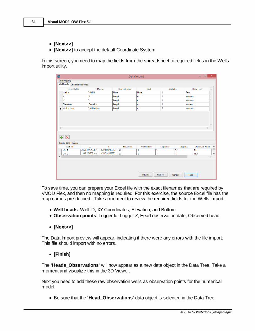
In this screen, you need to map the fields from the spreadsheet to required fields in the WellsImport utility.
To save time, you can prepare your Excel file with the exact filenames that are required byVMOD Flex, and then no mapping is required. For this exercise, the source Excel file has themap names pre-defined. Take a moment to review the required fields for the Wells import:
· Well heads: Well ID, XY Coordinates, Elevation, and Bottom
· Observation points: Logger Id, Logger Z, Head observation date, Observed head
· [Next>>]
The Data Import preview will appear, indicating if there were any errors with the file import.This file should import with no errors.
· [Finish]
The 'Heads_Observations' will now appear as a new data object in the Data Tree. Take amoment and visualize this in the 3D Viewer.
Next you need to add these raw observation wells as observation points for the numericalmodel.
· Be sure that the 'Head_Observations' data object is selected in the Data Tree.
Airport Numerical Model with Transport 32
© 2018 by Waterloo Hydrogeologic
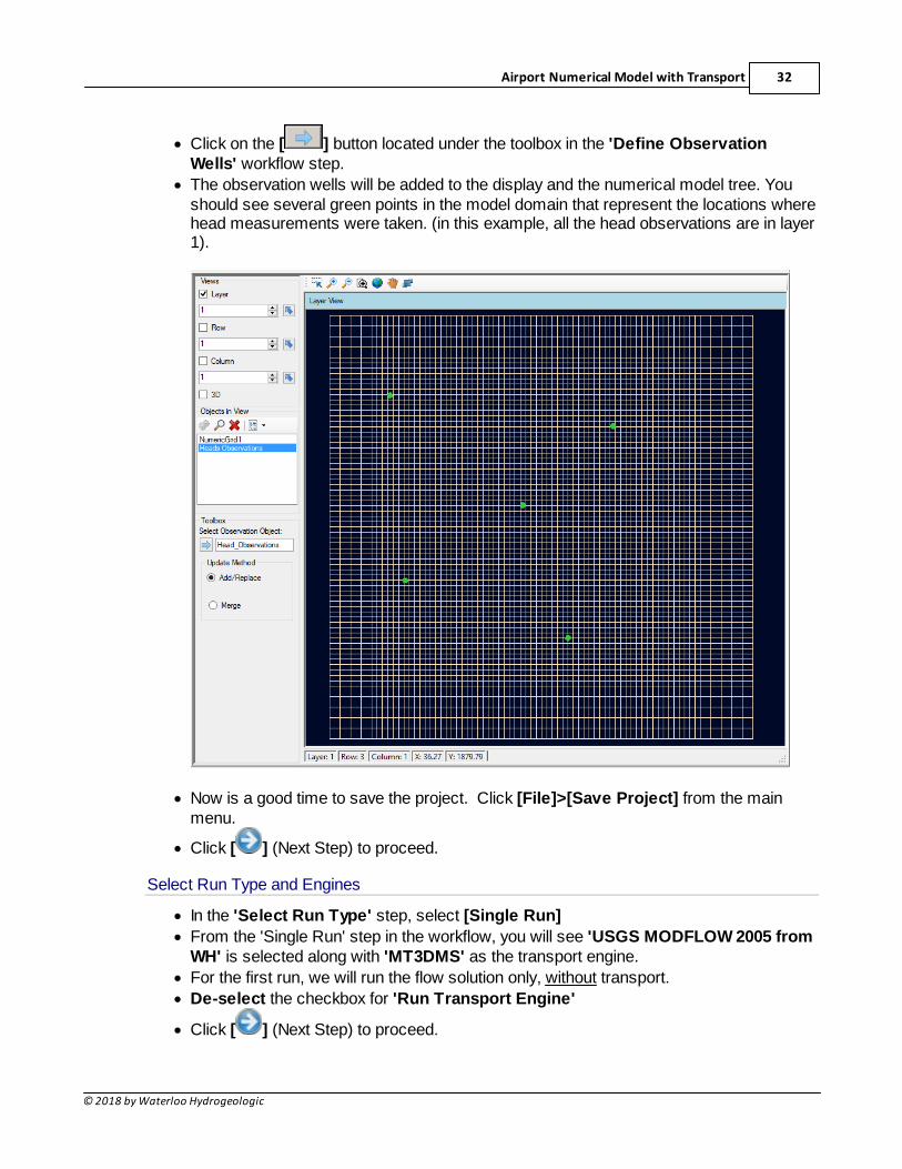
· Click on the [ ] button located under the toolbox in the 'Define ObservationWells' workflow step.
· The observation wells will be added to the display and the numerical model tree. Youshould see several green points in the model domain that represent the locations wherehead measurements were taken. (in this example, all the head observations are in layer1).
· Now is a good time to save the project. Click [File]>[Save Project] from the mainmenu.
· Click [ ] (Next Step) to proceed.
Select Run Type and Engines
· In the 'Select Run Type' step, select [Single Run]
· From the 'Single Run' step in the workflow, you will see 'USGS MODFLOW 2005 fromWH' is selected along with 'MT3DMS' as the transport engine.
· For the first run, we will run the flow solution only, without transport.
· De-select the checkbox for 'Run Transport Engine'
· Click [ ] (Next Step) to proceed.
Visual MODFLOW Flex 5.133
© 2018 by Waterloo Hydrogeologic
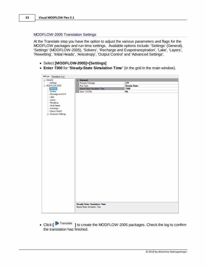
MODFLOW-2005 Translation Settings
At the Translate step you have the option to adjust the various parameters and flags for theMODFLOW packages and run time settings. Available options include: 'Settings' (General),'Settings' (MODFLOW-2005), 'Solvers', 'Recharge and Evapotranspiration', 'Lake', 'Layers','Rewetting', 'Initial Heads', 'Anisotropy', 'Output Control' and 'Advanced Settings'.
· Select [MODFLOW-2005]>[Settings]
· Enter 7300 for 'Steady-State Simulation Time' (in the grid in the main window).
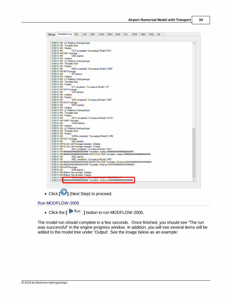
· Click [ ] to create the MODFLOW-2005 packages. Check the log to confirmthe translation has finished.
Airport Numerical Model with Transport 34
© 2018 by Waterloo Hydrogeologic
· Click [ ] (Next Step) to proceed.
Run MODFLOW-2005
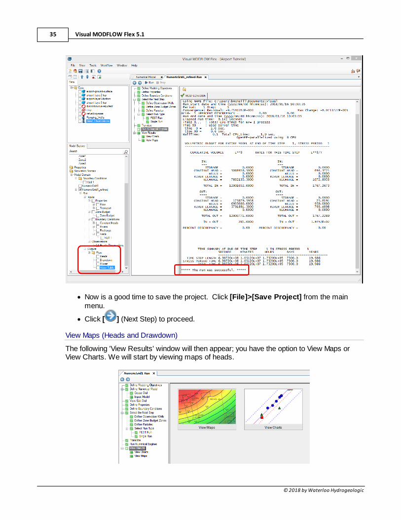
· Click the [ ] button to run MODFLOW-2005.
The model run should complete in a few seconds. Once finished, you should see "The runwas successful" in the engine progress window. In addition, you will see several items will beadded to the model tree under 'Output'. See the image below as an example:
Visual MODFLOW Flex 5.135
© 2018 by Waterloo Hydrogeologic
· Now is a good time to save the project. Click [File]>[Save Project] from the mainmenu.
· Click [ ] (Next Step) to proceed.
View Maps (Heads and Drawdown)
The following 'View Results' window will then appear; you have the option to View Maps orView Charts. We will start by viewing maps of heads.
Airport Numerical Model with Transport 36
© 2018 by Waterloo Hydrogeologic
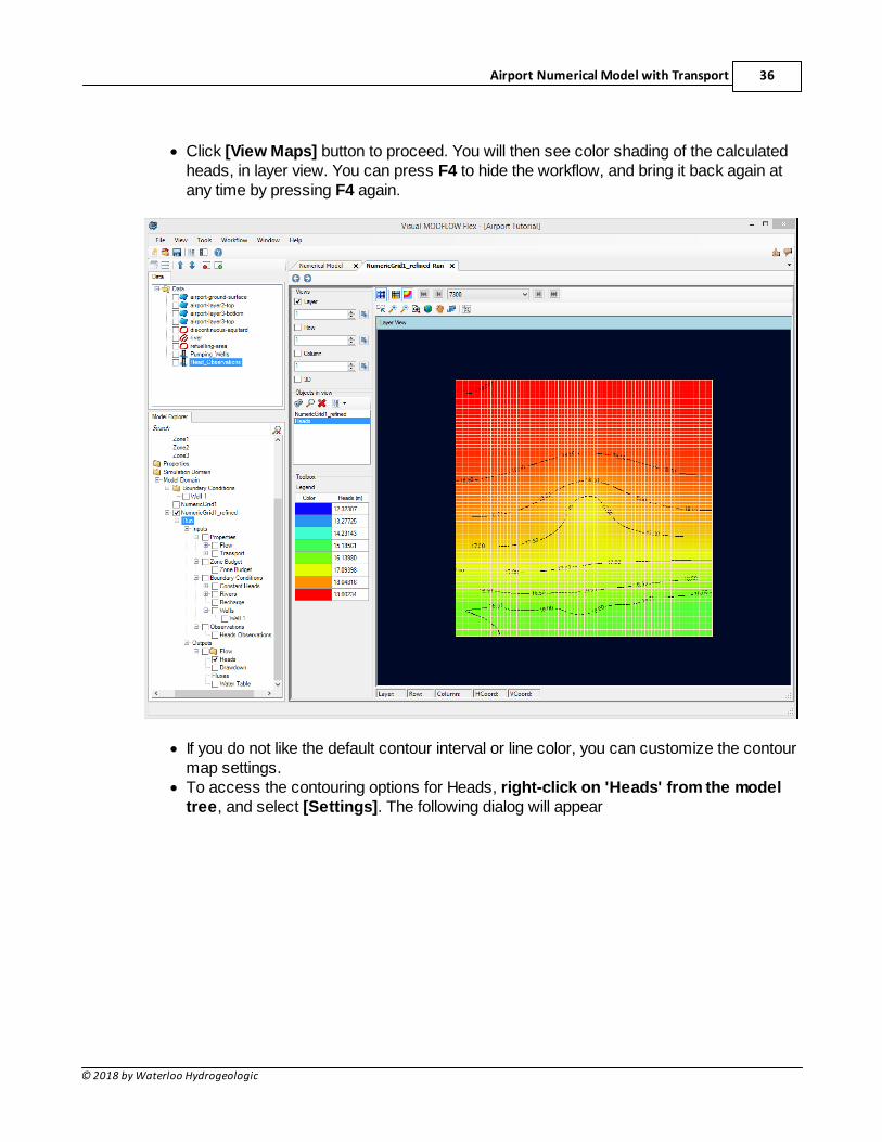
· Click [View Maps] button to proceed. You will then see color shading of the calculatedheads, in layer view. You can press F4 to hide the workflow, and bring it back again atany time by pressing F4 again.
· If you do not like the default contour interval or line color, you can customize the contourmap settings.
· To access the contouring options for Heads, right-click on 'Heads' from the modeltree, and select [Settings]. The following dialog will appear
Visual MODFLOW Flex 5.137
© 2018 by Waterloo Hydrogeologic
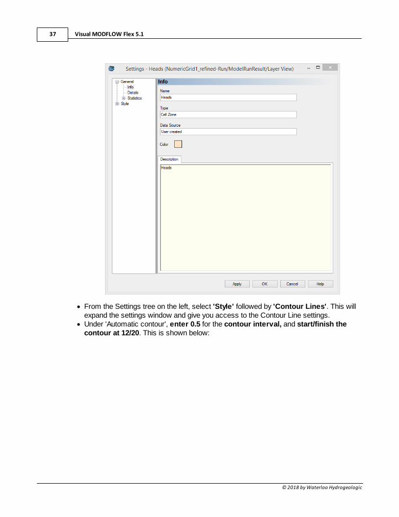
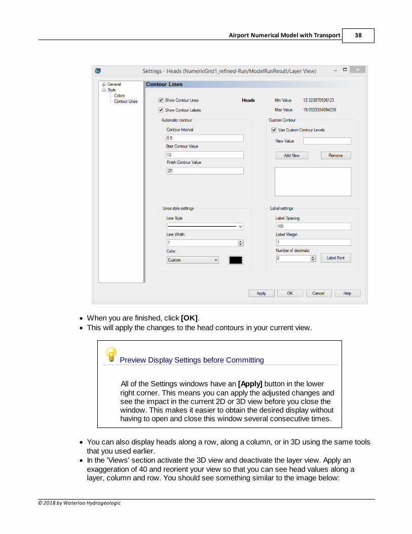
· From the Settings tree on the left, select 'Style' followed by 'Contour Lines'. This willexpand the settings window and give you access to the Contour Line settings.
· Under 'Automatic contour', enter 0.5 for the contour interval, and start/finish thecontour at 12/20. This is shown below:
Airport Numerical Model with Transport 38
© 2018 by Waterloo Hydrogeologic
· When you are finished, click [OK].
· This will apply the changes to the head contours in your current view.
Preview Display Settings before Committing
All of the Settings windows have an [Apply] button in the lowerright corner. This means you can apply the adjusted changes andsee the impact in the current 2D or 3D view before you close thewindow. This makes it easier to obtain the desired display withouthaving to open and close this window several consecutive times.
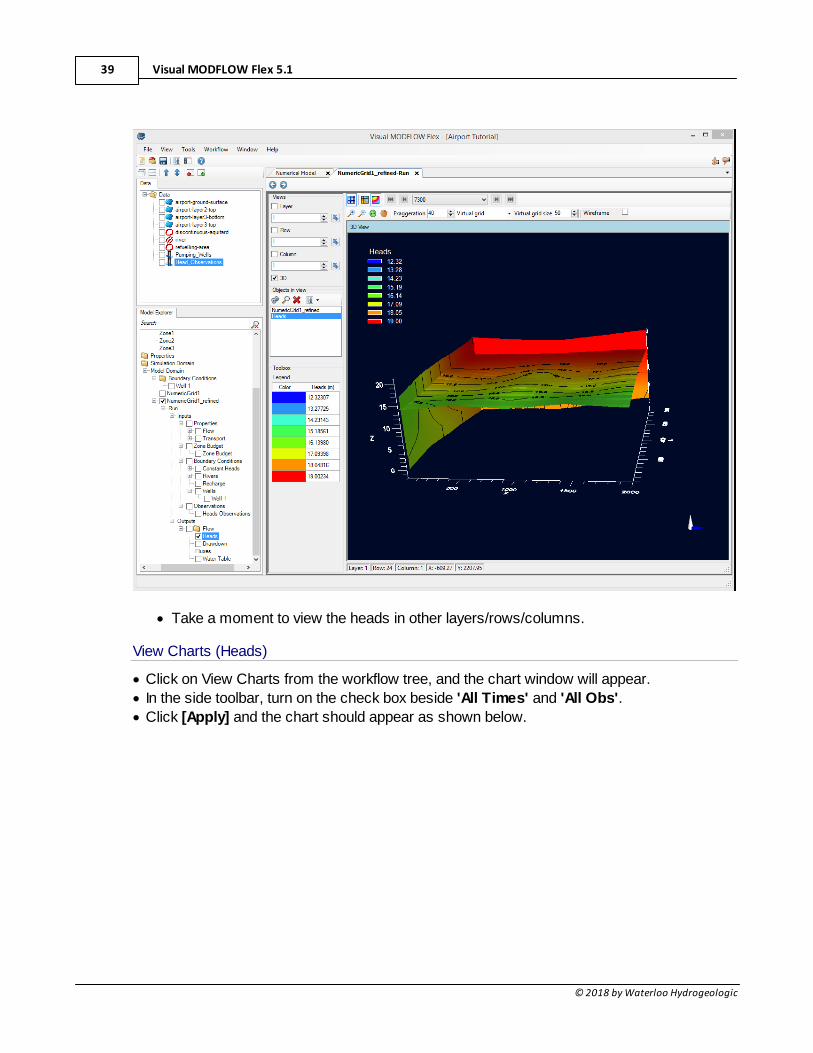
· You can also display heads along a row, along a column, or in 3D using the same toolsthat you used earlier.
· In the 'Views' section activate the 3D view and deactivate the layer view. Apply anexaggeration of 40 and reorient your view so that you can see head values along alayer, column and row. You should see something similar to the image below:
Visual MODFLOW Flex 5.139
© 2018 by Waterloo Hydrogeologic
· Take a moment to view the heads in other layers/rows/columns.
View Charts (Heads)
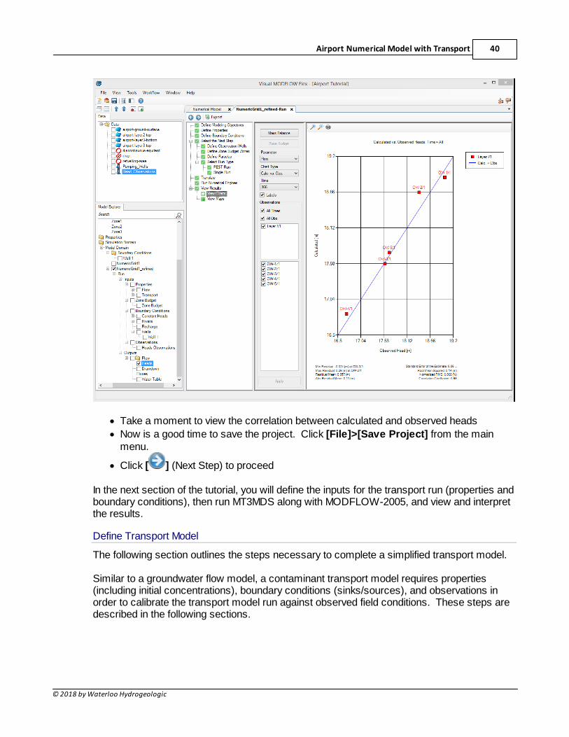
· Click on View Charts from the workflow tree, and the chart window will appear.
· In the side toolbar, turn on the check box beside 'All Times' and 'All Obs'.
· Click [Apply] and the chart should appear as shown below.
Airport Numerical Model with Transport 40
© 2018 by Waterloo Hydrogeologic
· Take a moment to view the correlation between calculated and observed heads
· Now is a good time to save the project. Click [File]>[Save Project] from the mainmenu.
· Click [ ] (Next Step) to proceed
In the next section of the tutorial, you will define the inputs for the transport run (properties andboundary conditions), then run MT3MDS along with MODFLOW-2005, and view and interpretthe results.
Define Transport Model
The following section outlines the steps necessary to complete a simplified transport model.
Similar to a groundwater flow model, a contaminant transport model requires properties(including initial concentrations), boundary conditions (sinks/sources), and observations inorder to calibrate the transport model run against observed field conditions. These steps aredescribed in the following sections.
Visual MODFLOW Flex 5.141
© 2018 by Waterloo Hydrogeologic
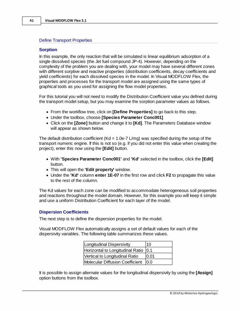
Define Transport Properties
Sorption
In this example, the only reaction that will be simulated is linear equilibrium adsorption of asingle dissolved species (the Jet fuel compound JP-4). However, depending on thecomplexity of the problem you are dealing with, your model may have several different zoneswith different sorptive and reactive properties (distribution coefficients, decay coefficients andyield coefficients) for each dissolved species in the model. In Visual MODFLOW Flex, theproperties and processes for the transport model are assigned using the same types ofgraphical tools as you used for assigning the flow model properties.
For this tutorial you will not need to modify the Distribution Coefficient value you defined duringthe transport model setup, but you may examine the sorption parameter values as follows.
· From the workflow tree, click on [Define Properties] to go back to this step.
· Under the toolbox, choose [Species Parameter Conc001]
· Click on the [Zone] button and change it to [Kd]. The Parameters Database windowwill appear as shown below.
The default distribution coefficient (Kd = 1.0e-7 L/mg) was specified during the setup of thetransport numeric engine. If this is not so (e.g. if you did not enter this value when creating theproject), enter this now using the [Edit] button.
· With 'Species Parameter Conc001' and 'Kd' selected in the toolbox, click the [Edit]button.
· This will open the 'Edit property' window.
· Under the 'Kd' column enter 1E-07 in the first row and click F2 to propagate this valueto the rest of the column.
The Kd values for each zone can be modified to accommodate heterogeneous soil propertiesand reactions throughout the model domain. However, for this example you will keep it simpleand use a uniform Distribution Coefficient for each layer of the model.
Dispersion Coefficients
The next step is to define the dispersion properties for the model.
Visual MODFLOW Flex automatically assigns a set of default values for each of thedispersivity variables. The following table summarizes these values.
Longitudinal Dispersivity 10
Horizontal to Longitudinal Ratio 0.1
Vertical to Longitudinal Ratio 0.01
Molecular Diffusion Coefficient 0.0
It is possible to assign alternate values for the longitudinal dispersivity by using the [Assign]option buttons from the toolbox.
Airport Numerical Model with Transport 42
© 2018 by Waterloo Hydrogeologic
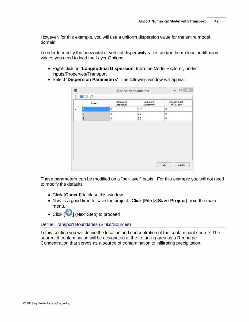
However, for this example, you will use a uniform dispersion value for the entire modeldomain.
In order to modify the horizontal or vertical dispersivity ratios and/or the molecular diffusionvalues you need to load the Layer Options.
· Right-click on 'Longitudinal Dispersion' from the Model Explorer, underInputs/Properties/Transport
· Select 'Dispersion Parameters'. The following window will appear:
These parameters can be modified on a "per-layer" basis. For this example you will not needto modify the defaults
· Click [Cancel] to close this window
· Now is a good time to save the project. Click [File]>[Save Project] from the mainmenu.
· Click [ ] (Next Step) to proceed
Define Transport Boundaries (Sinks/Sources)
In this section you will define the location and concentration of the contaminant source. Thesource of contamination will be designated at the refueling area as a RechargeConcentration that serves as a source of contamination to infiltrating precipitation.
Visual MODFLOW Flex 5.143
© 2018 by Waterloo Hydrogeologic
Transport Boundary Conditions: VMOD Flex vs. VMOD Classic
If you are used to working with Visual MODFLOW Classic, youwill notice a difference in how transport boundary conditions arehandled in Visual MODFLOW Flex. In VMOD Classic, transportboundary conditions were defined separately from the flowboundary conditions using the types Constant Concentration,Recharge Concentration, Evapotranspiration Concentration, andPoint Source. In Visual MODFLOW Flex, the sink/sourceparameters for transport models (which are time and speciesconcentrations) are defined as part of flow boundary conditions,which is a more natural representation. This means you do notdefine separate cell geometries for transport boundaries, yousimply define species concentrations while defining the flowboundary conditions, where required. Constant Concentration isan exception to this rule, since it does not need to coincide with aprescribed flux, you will still see a "Constant Concentration"boundary condition type, allowing you to define the geometry(cells) and parameters (time and species concentrations) for thisBoundary Condition type.
When Transport is active in your model run, and you define a newboundary condition, you will see parameters for SpeciesConcentration as part of the Boundary Condition attributes (eg.Conc001, Conc002, etc..). These will have a default value of -1,indicating that no mass sink/source is defined for this group ofboundary condition cells. As soon as you change this value to 0or greater, then these cells will be treated as sinks/sources
Assign Species Concentrations for the Recharge Boundary
When you defined the flow model, you created a separate recharge zone that covers therefuelling area. Now you will add a defined species concentration to this recharge flux.
· Check to ensure that you are viewing Layer 1.
· Select 'Recharge' from the list of available boundary conditions under the toolbox.
· You will recall there were two recharge zones created for the flow model: backgroundrecharge of 100 mm/yr covering the entire model top, and a small area over therefueling area with a higher recharge rate of 250 mm/yr. The mass of contaminants willbe assigned only to this smaller recharge zone.
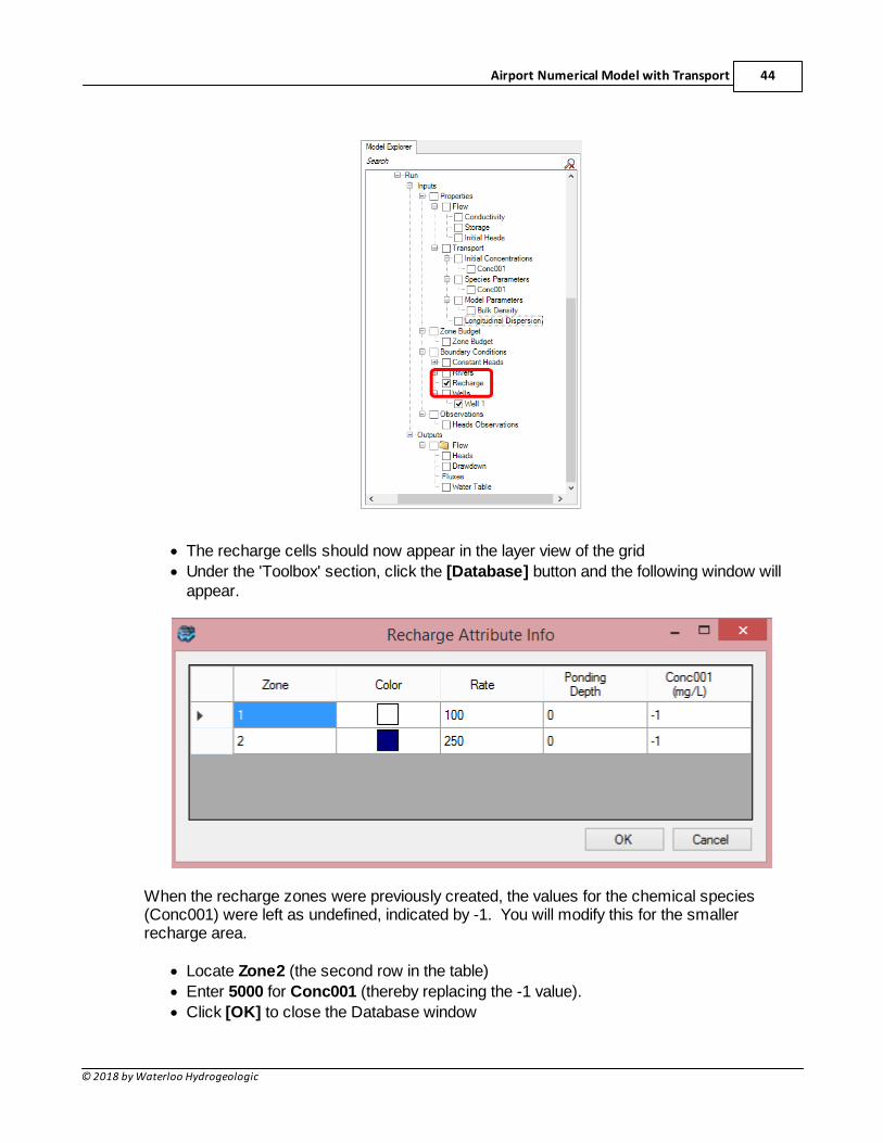
· If not already visible, you must make the Recharge zones visible. In the Model Explorer,locate the 'Recharge' node, under 'Inputs'>'Boundary Conditions', as shown below.
· Click on the box beside 'Recharge' in the tree .
Airport Numerical Model with Transport 44
© 2018 by Waterloo Hydrogeologic
· The recharge cells should now appear in the layer view of the grid
· Under the 'Toolbox' section, click the [Database] button and the following window willappear.
When the recharge zones were previously created, the values for the chemical species(Conc001) were left as undefined, indicated by -1. You will modify this for the smallerrecharge area.
· Locate Zone2 (the second row in the table)
· Enter 5000 for Conc001 (thereby replacing the -1 value).
· Click [OK] to close the Database window
Visual MODFLOW Flex 5.145
© 2018 by Waterloo Hydrogeologic
· Now is a good time to save the project. Click [File]>[Save Project] from the mainmenu.
· Click [ ] (Next Step) to proceed
· Select [Define Observation Wells]
Define Concentration Observations
The final step before running the transport simulation is to add the three observation wells tothe model to monitor the jet fuel concentrations at selected locations down-gradient of therefueling area. The first observation well (OW1) was installed immediately down-gradientof the refuelling area shortly after the refuelling operation started. The other two observationwells (OW2 and OW3) were installed two years later when elevated JP-4 concentrationswere observed at the first well (OW1).
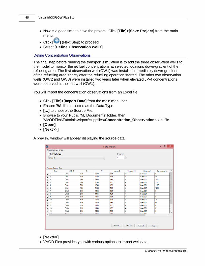
You will import the concentration observations from an Excel file.
· Click [File]>[Import Data] from the main menu bar
· Ensure 'Well' is selected as the Data Type
· […] to choose the Source File.
· Browse to your Public 'My Documents' folder, then'VMODFlex\Tutorials\Airport\suppfiles\Concentration_Observations.xls' file.
· [Open]
· [Next>>]
A preview window will appear displaying the source data.
· [Next>>]
· VMOD Flex provides you with various options to import well data.

Airport Numerical Model with Transport 46
© 2018 by Waterloo Hydrogeologic
· Choose the radio button [Well heads with the following data] radio button
· Then select [Observations points]
· Then select [Observed concentrations]
· [Next>>]
· [Next>>] to accept the default Coordinate System.
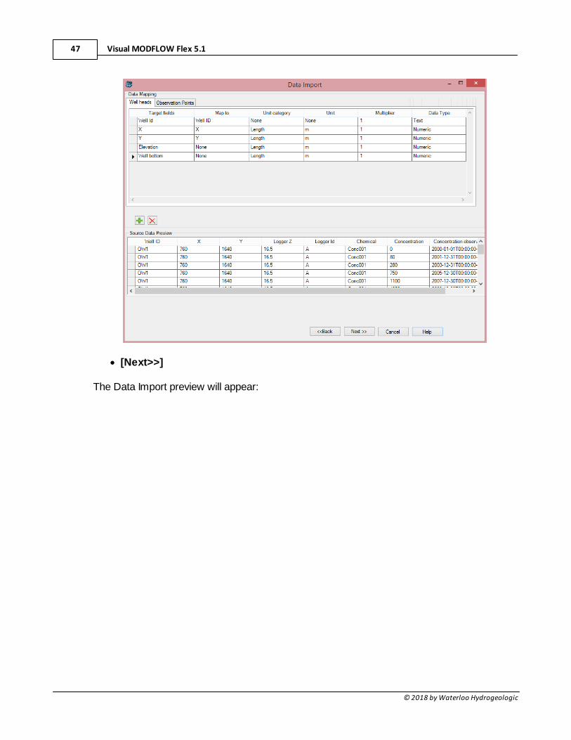
· In this screen, you need to map the fields from the spreadsheet to required fields in theDells Import utility. To save time, you can prepare your Excel file with the exactfilenames that are required by VMOD Flex, and then no mapping is required. For thisexercise, the source Excel file has the map names pre-defined. Take a moment toreview the required fields for the Wells import:
· Well Heads: Well ID, X/Y Coordinates, Elevation, and Well Bottom
· Observation Points: Logger Id, Logger Z, Concentration observation date, Observedconcentration
Visual MODFLOW Flex 5.147
© 2018 by Waterloo Hydrogeologic
· [Next>>]
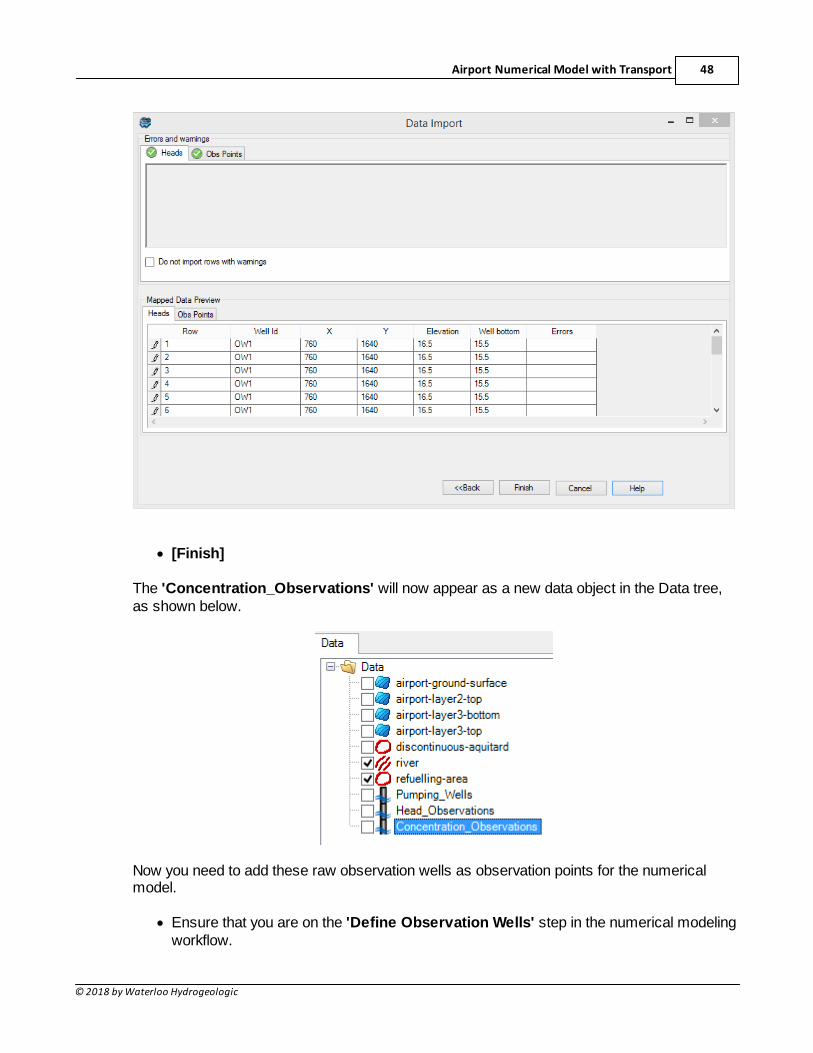
The Data Import preview will appear:
Airport Numerical Model with Transport 48
© 2018 by Waterloo Hydrogeologic
· [Finish]
The 'Concentration_Observations' will now appear as a new data object in the Data tree,as shown below.
Now you need to add these raw observation wells as observation points for the numericalmodel.
· Ensure that you are on the 'Define Observation Wells' step in the numerical modelingworkflow.
Visual MODFLOW Flex 5.149
© 2018 by Waterloo Hydrogeologic
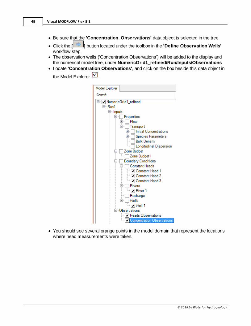
· Be sure that the 'Concentration_Observations' data object is selected in the tree
· Click the [ ] button located under the toolbox in the 'Define Observation Wells'workflow step.
· The observation wells ('Concentration Observations') will be added to the display andthe numerical model tree, under NumericGrid1_refined/Run/Inputs/Observations
· Locate 'Concentration Observations', and click on the box beside this data object in
the Model Explorer .
· You should see several orange points in the model domain that represent the locationswhere head measurements were taken.
Airport Numerical Model with Transport 50
© 2018 by Waterloo Hydrogeologic
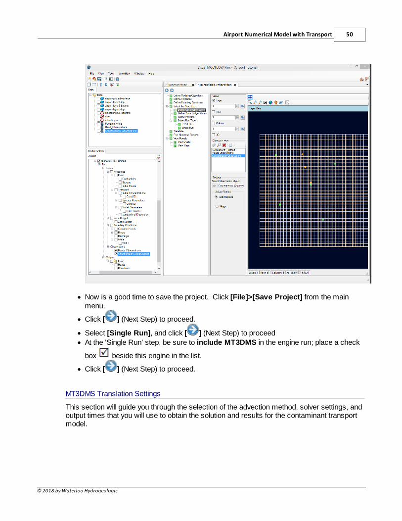
· Now is a good time to save the project. Click [File]>[Save Project] from the mainmenu.
· Click [ ] (Next Step) to proceed.
· Select [Single Run], and click [ ] (Next Step) to proceed
· At the 'Single Run' step, be sure to include MT3DMS in the engine run; place a check
box beside this engine in the list.
· Click [ ] (Next Step) to proceed.
MT3DMS Translation Settings
This section will guide you through the selection of the advection method, solver settings, andoutput times that you will use to obtain the solution and results for the contaminant transportmodel.

Visual MODFLOW Flex 5.151
© 2018 by Waterloo Hydrogeologic
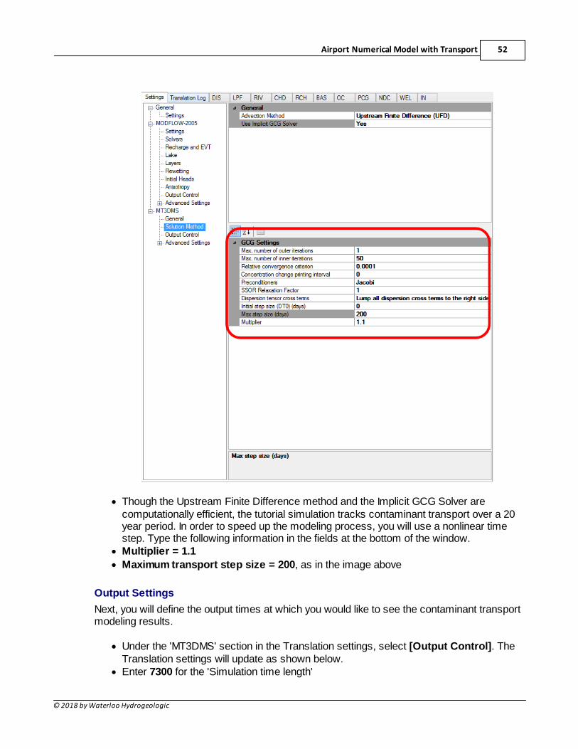
Solution Method
· Expand the 'MT3DMS' item under the Translation settings, and select [SolutionMethod]. A Solution Method settings window will appear.
For this model run you will be using the Upstream Finite Difference solution method with theImplicit GCG Solver. The Upstream Finite Difference method provides a stable solution to thecontaminant transport model in a relatively short period of time. The GCG solver uses animplicit approach to solving the finite difference equations, and is usually much faster than theexplicit solution method.
· Click the button in the 'Advection Method' option and select [Upstream FiniteDifference (UFD)]
· Click the button in the 'Use Implicit GCG Solver' option and select [Yes].
· The Implicit GCG Solver Settings window will appear in the lower half of the translationsettings window, as shown in the image below:
Airport Numerical Model with Transport 52
© 2018 by Waterloo Hydrogeologic
· Though the Upstream Finite Difference method and the Implicit GCG Solver arecomputationally efficient, the tutorial simulation tracks contaminant transport over a 20year period. In order to speed up the modeling process, you will use a nonlinear timestep. Type the following information in the fields at the bottom of the window.
· Multiplier = 1.1
· Maximum transport step size = 200, as in the image above
Output Settings
Next, you will define the output times at which you would like to see the contaminant transportmodeling results.
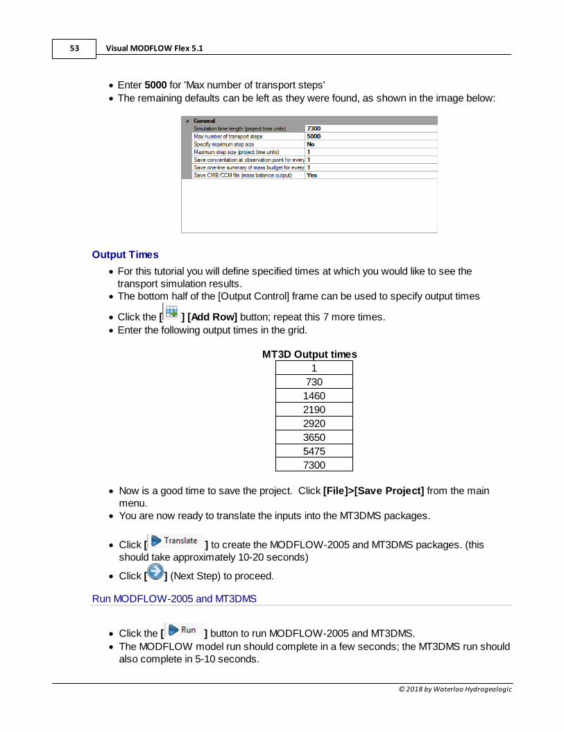
· Under the 'MT3DMS' section in the Translation settings, select [Output Control]. TheTranslation settings will update as shown below.
· Enter 7300 for the 'Simulation time length'
Visual MODFLOW Flex 5.153
© 2018 by Waterloo Hydrogeologic
· Enter 5000 for 'Max number of transport steps'
· The remaining defaults can be left as they were found, as shown in the image below:
Output Times
· For this tutorial you will define specified times at which you would like to see thetransport simulation results.
· The bottom half of the [Output Control] frame can be used to specify output times
· Click the [ ] [Add Row] button; repeat this 7 more times.
· Enter the following output times in the grid.
MT3D Output times
1
730
1460
2190
2920
3650
5475
7300
· Now is a good time to save the project. Click [File]>[Save Project] from the mainmenu.
· You are now ready to translate the inputs into the MT3DMS packages.
· Click [ ] to create the MODFLOW-2005 and MT3DMS packages. (thisshould take approximately 10-20 seconds)
· Click [ ] (Next Step) to proceed.
Run MODFLOW-2005 and MT3DMS
· Click the [ ] button to run MODFLOW-2005 and MT3DMS.
· The MODFLOW model run should complete in a few seconds; the MT3DMS run shouldalso complete in 5-10 seconds.
Airport Numerical Model with Transport 54
© 2018 by Waterloo Hydrogeologic
· Once finished, you should see "***** The run was successful. *****" in the engineprogress window.
· In addition, you will see several items will be added to the model tree under 'Outputs'. You should also see 'Concentrations' added to the model output tree under'Output/Transport'.
· Now is a good time to save the project. Click [File]>[Save Project] from the mainmenu.
· Click [ ] (Next Step) to proceed.
· Click [View Maps].
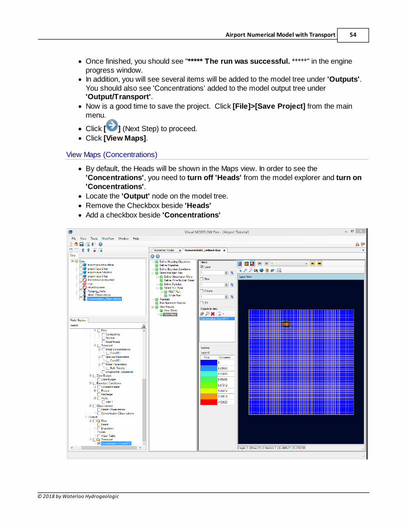
View Maps (Concentrations)
· By default, the Heads will be shown in the Maps view. In order to see the'Concentrations', you need to turn off 'Heads' from the model explorer and turn on'Concentrations'.
· Locate the 'Output' node on the model tree.
· Remove the Checkbox beside 'Heads'
· Add a checkbox beside 'Concentrations'
Visual MODFLOW Flex 5.155
© 2018 by Waterloo Hydrogeologic
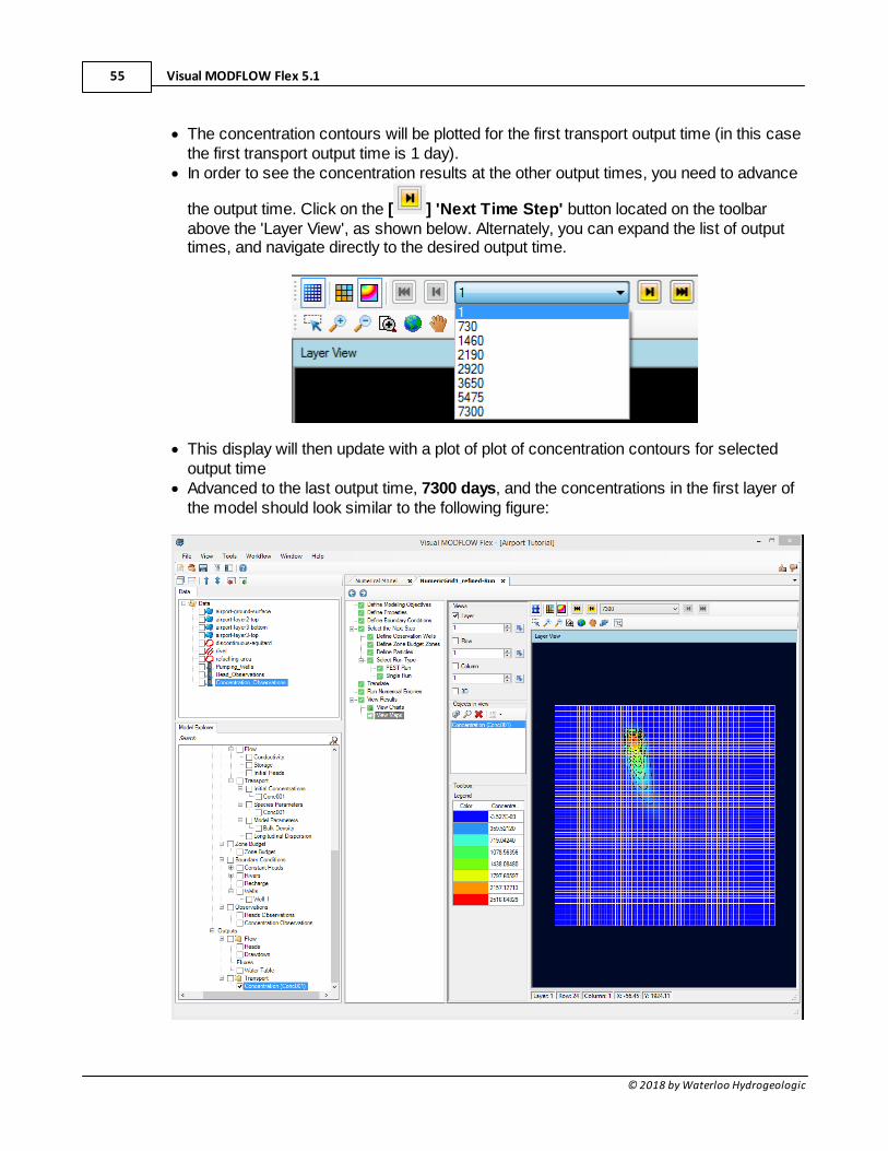
· The concentration contours will be plotted for the first transport output time (in this casethe first transport output time is 1 day).
· In order to see the concentration results at the other output times, you need to advance
the output time. Click on the [ ] 'Next Time Step' button located on the toolbarabove the 'Layer View', as shown below. Alternately, you can expand the list of outputtimes, and navigate directly to the desired output time.
· This display will then update with a plot of plot of concentration contours for selectedoutput time
· Advanced to the last output time, 7300 days, and the concentrations in the first layer ofthe model should look similar to the following figure:
Airport Numerical Model with Transport 56
© 2018 by Waterloo Hydrogeologic
· You can determine the risk that the contaminant front poses to the discontinuousaquitard by doing the following:
· Locate the data object "discontinuous-aquitard" from the tree, and turn it on. It shouldappear in the layer view. Take a moment to navigate through the other layers, to seethe calculated concentrations.
· Move your mouse cursor to specific areas of the interest (such as in the discontinuousaquitard region), and note in the status bar the calculated concentrations for theselected cell.
· After 7300 days (20 years) of simulation time it is clear that the plume has migrated tothe ‘hole’ in the aquitard.
· To see how the plume looks in cross-section, turn on the [Column] view, and entercolumn 25
· Advance the times to see the plume migrating the upper layers down to the lowerlayers.
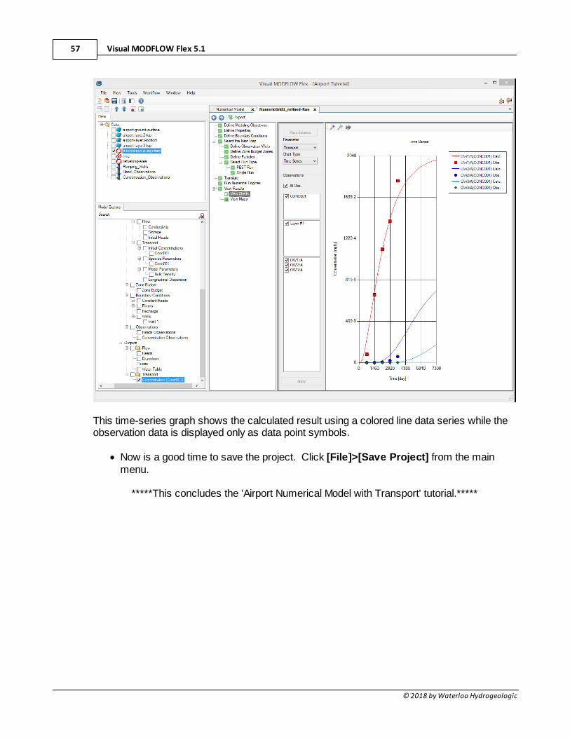
View Charts (Concentrations)
In this section you will learn how to compare the observed concentration data to theconcentration values calculated by the model.
· Select [View Charts] item from the workflow tree.
· From the 'Parameter' combo box to the left of the main chart window, choose'Transport'
· Then, under 'Chart Type' select 'Time Series'
· Select 'All Times' and 'All Obs.' from the 'Observations' frame on the left side of thewindow
· Click [Apply]
· You should now be viewing the breakthrough curves for each of the three concentrationobservation wells defined earlier in the model (see following figure).
Visual MODFLOW Flex 5.157
© 2018 by Waterloo Hydrogeologic
This time-series graph shows the calculated result using a colored line data series while theobservation data is displayed only as data point symbols.
· Now is a good time to save the project. Click [File]>[Save Project] from the mainmenu.
*****This concludes the 'Airport Numerical Model with Transport' tutorial.*****