Embed Size (px)
Citation preview

University of Illinois at Urbana-ChampaignBeckman Institute for Advanced Science and TechnologyTheoretical and Computational Biophysics GroupComputational Biophysics Workshop
Using VMD
VMD Developer:John Stone
Tutorial Contributors:Alek Aksimentiev, Anton Arkhipov, Robert Brunner, JordiCohen, Brijeet Dhaliwal, John Eargle, Jen Hsin, Fatemeh Khalili,Eric H. Lee, Zan Luthey-Schulten, Patrick O’Donoghue, ElijahRoberts, Anurag Sethi, Marcos Sotomayor, Emad Tajkhorshid,Leonardo Trabuco, Elizabeth Villa, Yi Wang, David Wells, DanWright, Ying Yin
July 2009

2
A current version of this tutorial is available at
http://www.ks.uiuc.edu/Training/Tutorials/
Join the [email protected] mailing list for additional help.

CONTENTS 3
Contents
1 Working with a Single Molecule 81.1 Loading a Molecule . . . . . . . . . . . . . . . . . . . . . . . . . . 81.2 Displaying the Molecule . . . . . . . . . . . . . . . . . . . . . . . 91.3 Graphical Representations . . . . . . . . . . . . . . . . . . . . . . 10
1.3.1 Exploring different drawing styles . . . . . . . . . . . . . . 101.3.2 Exploring different coloring methods . . . . . . . . . . . . 121.3.3 Displaying different selections . . . . . . . . . . . . . . . . 131.3.4 Creating multiple representations . . . . . . . . . . . . . . 14
1.4 Sequence Viewer Extension . . . . . . . . . . . . . . . . . . . . . 151.5 Saving Your Work . . . . . . . . . . . . . . . . . . . . . . . . . . 171.6 The Basics of VMD Figure Rendering . . . . . . . . . . . . . . . 18
1.6.1 Setting the display background . . . . . . . . . . . . . . . 181.6.2 Increasing resolution . . . . . . . . . . . . . . . . . . . . . 181.6.3 Colors and materials . . . . . . . . . . . . . . . . . . . . . 191.6.4 Depth perception . . . . . . . . . . . . . . . . . . . . . . . 211.6.5 Rendering . . . . . . . . . . . . . . . . . . . . . . . . . . . 23
2 Trajectories and Movie Making 252.1 Loading Trajectories . . . . . . . . . . . . . . . . . . . . . . . . . 252.2 Main Menu Animation Tools . . . . . . . . . . . . . . . . . . . . 262.3 Trajectory Visualization . . . . . . . . . . . . . . . . . . . . . . . 27
2.3.1 Smoothing trajectories . . . . . . . . . . . . . . . . . . . . 272.3.2 Displaying multiple frames . . . . . . . . . . . . . . . . . 272.3.3 Updating selections . . . . . . . . . . . . . . . . . . . . . 28
2.4 The Basics of Move Making in VMD . . . . . . . . . . . . . . . . 292.4.1 Making single-frame movies . . . . . . . . . . . . . . . . . 302.4.2 Making trajectory movies . . . . . . . . . . . . . . . . . . 30
3 Scripting in VMD 323.1 The Basics of Tcl Scripting . . . . . . . . . . . . . . . . . . . . . 323.2 VMD scripting . . . . . . . . . . . . . . . . . . . . . . . . . . . . 34
3.2.1 Loading molecules with text commands . . . . . . . . . . 343.2.2 The atomselect command . . . . . . . . . . . . . . . . . 353.2.3 Obtaining and changing molecule properties with text
commands . . . . . . . . . . . . . . . . . . . . . . . . . . . 353.2.4 Sourcing scripts . . . . . . . . . . . . . . . . . . . . . . . . 39
3.3 Drawing shapes . . . . . . . . . . . . . . . . . . . . . . . . . . . . 40

CONTENTS 4
4 Working with Multiple Molecules 424.1 Main Menu Molecule List Browser . . . . . . . . . . . . . . . . . 42
4.1.1 Loading multiple molecules . . . . . . . . . . . . . . . . . 424.1.2 Changing molecule names . . . . . . . . . . . . . . . . . . 434.1.3 Drawing different representations for different molecules . 444.1.4 Molecule Status Flags . . . . . . . . . . . . . . . . . . . . 44
4.2 Aligning Molecules with the measure fit Command . . . . . . . 46
5 Comparing Structures and Sequences with MultiSeq 485.1 Structure Alignment with MultiSeq . . . . . . . . . . . . . . . . . 48
5.1.1 Loading aquaporin structures . . . . . . . . . . . . . . . . 485.1.2 Aligning the molecules . . . . . . . . . . . . . . . . . . . . 495.1.3 Coloring molecules by their structural identity . . . . . . 52
5.2 Sequence Alignment with MultiSeq . . . . . . . . . . . . . . . . . 525.2.1 Aligning molecules and coloring molecules by degree of
conservation . . . . . . . . . . . . . . . . . . . . . . . . . . 535.2.2 Importing FASTA files for sequence alignment . . . . . . 53
5.3 Phylogenetic Tree . . . . . . . . . . . . . . . . . . . . . . . . . . . 56
6 Data Analysis in VMD 586.1 Labels . . . . . . . . . . . . . . . . . . . . . . . . . . . . . . . . . 586.2 Example of a built-in analysis tool: the RMSD Trajectory Tool . 606.3 Example of an analysis script . . . . . . . . . . . . . . . . . . . . 63

CONTENTS 5
Introduction
VMD (Visual Molecular Dynamics) is a molecular visualization and analysisprogram designed for biological systems such as proteins, nucleic acids, lipidbilayer assemblies, etc. It is developed by the Theoretical and ComputationalBiophysics Group at the University of Illinois at Urbana-Champaign. Amongmolecular graphics programs, VMD is unique in its ability to efficiently operateon multi-gigabyte molecular dynamics trajectories, its interoperability with alarge number of molecular dynamics simulation packages, and its integration ofstructure and sequence information.
Figure 1: Example VMD renderings.
Key features of VMD include:
• General 3-D molecular visualization with extensive drawing and coloringmethods
• Extensive atom selection syntax for choosing subsets of atoms for display
• Visualization of dynamic molecular data
• Visualization of volumetric data
• Supports all major molecular data file formats
• No limits on the number of molecules or trajectory frames, except availablememory
• Molecular analysis commands
• Rendering high-resolution, publication-quality molecule images
• Movie making capability
• Building and preparing systems for molecular dynamics simulations
• Interactive molecular dynamics simulations
• Extensions to the Tcl/Python scripting languages
• Extensible source code written in C and C++

CONTENTS 6
This article will serve as an introductory VMD tutorial. It is impossibleto cover all of VMD’s capabilities, but here we will present several step-by-step examples of VMD’s basic features. Topics covered in this tutorial includevisualizing molecules in three dimensions with different drawing and coloringmethods, rendering publication-quality figures, animate and analyze the trajec-tory of a molecular dynamics simulation, scripting in the text-based Tcl/Tkinterface, and analyzing both sequence and structure data for proteins.
Downloading VMD
Before staring the tutorial you need to download the current version of VMD.This tutorial uses VMD version 1.8.6. VMD supports all major computer plat-forms and can be obtained from the VMD development homepagehttp://www.ks.uiuc.edu/Research/vmd. Follow the instruction online to installVMD in your computer. Once VMD is installed, to start VMD:
• Mac OS X: Double click on the VMD application icon in the Applicationsdirectory.
• Linux and SUN: Type vmd in a terminal window.
• Windows: Select Start → Programs → VMD.
When VMD starts, by default three windows will open (Fig. 2): the VMD Mainwindow, the OpenGL Display window, and the VMD Console window (or aTerminal window on a Mac). To end a VMD session, go to the VMD Mainwindow, and choose File → Quit. You can also quit VMD by closing the VMDConsole window or the VMD Main window.
Figure 2: The VMD Main window, the OpenGL Display window, and the VMDConsole window.

CONTENTS 7
Tutorial Topics and Files
The tutorial contains six sections. Each section acts as an independent tutorialfor a specific topic, with the section layout as shown in Contents. For readerswith no prior experience with VMD, we suggest they work through the sectionsin the order they are presented. For readers already familiar with the basics ofVMD, they may selectively pursue sections of their interest. Several files havebeen prepared to accompany this tutorial. You need to download these filesat http://www.ks.uiuc.edu/Training/Tutorials/vmd. The files needed for eachchapter is illustrated in Fig. 3.
1 Working with a Single Molecule 1ubq.pdb
2 Trajectories and Movie Making ubiquitin.psf pulling.dcd
3 Scripting in VMD 1ubq.pdb beta.tcl
4 Working with Multiple Molecules 1fqy.pdb 1rc2.pdb
5. Comparing Protein Structures and Sequences with the MultiSeq Plugin 1fqy.pdb 1rc2.pdb 1lda.pdb 1j4n.pdb spinach_aqp.fasta
6 Data Analysis in VMD ubiquitin.psf pulling.dcd equilibration.dcd distance.tcl
Figure 3: The files needed for each section. All files are con-tained in the vmd-tutorial-files folder, which can be downloadedfrom http://www.ks.uiuc.edu/Training/Tutorials/vmd.

1 WORKING WITH A SINGLE MOLECULE 8
1 Working with a Single Molecule
In this section you will learn the basic functions of VMD. We will start withloading a molecule, displaying the molecule, and rendering publication-qualitymolecule images. This section uses the protein ubiquitin as an example molecule.Ubiquitin is a small protein responsible for labeling proteins for degradation, andis found in all eukaryotes with nearly identical sequences and structures.
1.1 Loading a Molecule
The first step is to load our molecule. A pdb file, 1ubq.pdb (Vijay-Kumar etal., JMB, 194:531, 1987), that contains the atom coordinates of ubiquitin isprovided with the tutorial.
Figure 4: Loading a Molecule.
1 Start a VMD session. In theVMD Main window, choose File
→ New Molecule... (Fig. 4(a)).Another window, the MoleculeFile Browser window (Fig. 4(b)),will appear on your screen.
2 Use the Browse... (Fig. 4(c))button to find the file 1ubq.pdbin vmd-tutorial-files direc-tory. Note that when you se-lect the file, you will be back inthe Molecule File Browser win-dow. In order to actually loadthe file you have to press Load
(Fig. 4(d)). Do not forget to do this!
Now, ubiquitin is shown in the OpenGL Display window. You may close theMolecule File Browser window at any time.
Webpdb. VMD can download a pdb file from the Protein Data
Bank1if a network connection is available. Just type the four letter
code of the protein in the File Name text entry of the Molecule File
Browser window and press the Load button. VMD will download it
automatically.
1Protein Data Bank website: http://www.pdb.org

1 WORKING WITH A SINGLE MOLECULE 9
1.2 Displaying the Molecule
In order to see the 3D structure of our protein, we will use the mouse in multiplemodes to change the viewpoint. VMD allows users to rotate, scale and translatethe viewpoint of your molecule.
Figure 5: Rotation modes. (a) Rotationaxes when holding down the left mousekey. (b) The rotation axis when holdingdown the right mouse key.
1 In the OpenGL Display, pressthe left mouse button down andmove the mouse. Explore whathappens. This is the rota-tion mode of the mouse and al-lows you to rotate the moleculearound an axis parallel to thescreen (Fig. 5(a)).
2 If you hold down the rightmouse button and repeat theprevious step, the rotation willbe done around an axis per-pendicular to your screen (Fig.5(b)) (For Mac users, the rightmouse button is equivalent to holding down the command key while press-ing the mouse button).
3 In the VMD Main window, look at the Mouse menu (Fig. 6). Here, youwill be able to switch the mouse mode from Rotation to Translation orScale modes.
Figure 6: Mouse modes and their char-acteristic cursors.
4 Choose the Translation modeand go back to the OpenGLDisplay. You can now move themolecule around when you holdthe left mouse button down.
5 Go back to the the Mouse menuand choose the Scale mode thistime. This will allow you tozoom in or out by moving themouse horizontally while hold-ing the left mouse button down.
It should be noted that these actionsperformed with the mouse only change your viewpoint and do not change theactual coordinates of the molecule atoms.

1 WORKING WITH A SINGLE MOLECULE 10
Mouse modes. Note that each mouse mode has its own charac-
teristic cursor and its own shortcut key (r: Rotate, t: Translate,
s: Scale). When you are in the OpenGL Display window, you can
use these shortcut keys instead of the Mouse menu to change the
mouse mode.
Another useful option is the Mouse → Center menu item. It allows you to specifythe point around which rotations are done.
6 Select the Center menu item and pick one atom at one of the ends of theprotein; The cursor should display a cross.
7 Now, press r, rotate the molecule with the mouse and see how yourmolecule moves around the point you have selected.
8 In the VMD Main window, select the Display → Reset View menu item toreturn to the default view. You can also reset the view by pressing the“=” key when you are in the OpenGL Display window.
1.3 Graphical Representations
VMD can display your molecule in various ways by the Graphical Representations
shown in Fig. 7. Each representation is defined by four main parameters: theselection of atoms included in the representation, the drawing style, the coloringmethod, and the material. The selection determines which part of the moleculeis drawn, the drawing method defines which graphical representation is used,the coloring method gives the the color of each part of the representation, andthe material determines the effects of lighting, shading, and transparency onthe representation. Let’s first explore different drawing styles.
1.3.1 Exploring different drawing styles
1 In the VMD Main window, choose the Graphics → Representations... menuitem. A window called Graphical Representations will appear and you willsee highlighted in yellow (Fig. 7(a)) the current default representationdisplaying your molecule.
2 In the Draw Style tab (Fig. 7(b)) we can change the style (Fig. 7(d)) andcolor (Fig. 7(c)) of the representation. In this section we will focus in thedrawing style (the default is Lines).
3 Each Drawing Method has its own parameters. For instance, change theThickness of the lines by using the controls on the lower right-hand-sidecorner (Fig. 7(c)) of the Graphical Representations window.

1 WORKING WITH A SINGLE MOLECULE 11
Figure 7: The Graphical Representa-tions window.
4 Click on the Drawing Method
(Fig. 7(d)), and you will see alist of options. Choose VDW
(van der Waals). Each atomis now represented by a sphere,allowing you to see more eas-ily the volumetric distributionof the protein.
5 When you choose VDW fordrawing method, two new con-trols would show up in the lowerright-hand-side corner (Fig. 7(e)).Use these controls to changethe Sphere Scale to 0.5 and theSphere Resolution to 13. Beaware that the higher the res-olution, the slower the displayof your molecule will be.
6 Press the Default button. Thisallows you to return to the de-fault properties of the chosendrawing method.
The previous representations al-low you to see the micromolecular details of your protein by displaying everysingle atom. More general structural properties can be demonstrated better byusing more abstract drawing methods.
7 Choose the Tube style under Drawing Method and observe the backboneof your protein. Set the Radius at 0.8. You should get something similarto Fig. 8.
8 By looking at your protein in the tube drawing method, see if you candistinguish the helices, β-sheets and coils present in the protein.
More representations. Other popular representations are CPK and
Licorice. In CPK, like in old chemistry ball & stick kits, each atom
is represented by a sphere and each bond is represented by a thin
cylinder (radius and resolution of both the sphere and the cylinder
can be modified independently). The Licorice drawing method also
represents each atom as a sphere and each bond as a cylinder, but
the sphere radius cannot be modified independently.

1 WORKING WITH A SINGLE MOLECULE 12
Figure 8: Licorice (left), Tube (center) and NewCartoon (right) representationsof Ubiquitin
The last drawing method we will explore is NewCartoon. It gives a simplifiedrepresentation of a protein based in its secondary structure. Helices are drawn ascoiled ribbons, β-sheets as solid arrows and all other structures as a tube. Thisis probably the most popular drawing method to view the overall architectureof a protein.
9 In the Graphical Representations window, choose Drawing Method→ New-
Cartoon. You can now easily identify how many helices, β-sheets and coilsare present in the protein.
Structure of ubiquitin. Ubiquitin has three and one half turns of
α-helix (residues 23 to 34, three of them hydrophobic), one short
piece of 310-helix (residues 56 to 59) and a mixed β-sheet with five
strands (residues 1 to 7, 10 to 17, 40 to 45, 48 to 50, and 64 to 72)
and seven reverse turns. VMD uses the program STRIDE (Frishman
et al., Proteins, 23:566, 1995) to compute the secondary structure
according to an heuristic algorithm.
1.3.2 Exploring different coloring methods
Now, let’s explore different coloring methods for our representations.
10 In the Graphical Representations window, you can see that the defaultcoloring method is Coloring Method → Name. In this coloring method, ifyou choose a drawing method that shows individual atoms, you can seethat they have different colors, i.e: O is red, N is blue, C is cyan and S isyellow.

1 WORKING WITH A SINGLE MOLECULE 13
11 Choose Coloring Method → ResType (Fig. 7(c)). This allows you to dis-tinguish non-polar residues (white), basic residues (blue), acidic residues(red) and polar residues (green).
12 Select Coloring Method → Structure (Fig. 7(c)) and confirm that the New-
Cartoon representation displays colors consistent with secondary structure.
1.3.3 Displaying different selections
You can also only display parts of the molecule that you are interested in byspecifying you selection in the Graphical Representations window (Fig. 7(f)).
Figure 9: Graphical Representationswindow and the Selections tab.
13 In the Graphical Representa-tions window, there is a Selected
Atoms text entry (Fig. 7(f)).Delete the word all, typehelix and press the Apply but-ton or hit the Enter/Return keyon your keyboard (remember todo this whenever you changea selection). VMD will showjust the helices present in ourmolecule.
14 In the Graphical Representa-tions window choose the Selec-
tions tab (Fig. 9(a)). In sectionSinglewords (Fig. 9(b)), you willfind a list of possible selectionsyou can type. For instance, tryto display β-sheets instead ofhelices by typing the appropri-ate word in the Selected Atoms
text entry.
Combinations of boolean operatorscan also be used when writing a se-lection.
15 In order to see the molecule without helices and β-sheets, type the follow-ing in Selected Atoms: (not helix) and (not betasheet). Rememberto press the Apply button or hit the Enter/Return key on your keyboard.
16 In the section Keyword (Fig. 9(c)) of the Selections tab, you can see proper-ties that can be used to select parts of a protein with their possible values.

1 WORKING WITH A SINGLE MOLECULE 14
Look at possible values of the keyword resname (Fig. 9(d)). Display all thelysines and glycines present in the protein by typing (resname LYS) or
(resname GLY) in the Selected Atoms. Lysines play a fundamental role inthe configuration of polyubiquitin chains.
17 Now, change the current representation’s Drawing Method to CPK and theColoring Method to ResName in the Draw Style tab. In the screen you willbe able to see the different Lysines and Glycines.
18 In the Selected Atoms text entry type water. Choose Coloring Method →Name. You should see the 58 water molecules (in fact only the oxygens)present in our system.
19 In order to see which water molecules are closer to the protein you canuse the command within. Type water and within 3 of protein forSelected Atoms. This selects all the water molecules that are within adistance of 3 angstroms of the protein.
20 Finally, try typing the following selections in Selected Atoms:
Selection Actionprotein Shows the Proteinresid 1 The first residue(resid 1 76) and (not water) The first and last residues(resid 23 to 34) and (protein) The α-helix
Table 1: Example atom selections.
1.3.4 Creating multiple representations
The button Create Rep (Fig. 10(a)) in the Graphical Representations windowallows you to create multiple representations. Therefore, you can have a mixtureof different selections with different styles and colors, all displayed at the sametime.
21 For the current representation, in Selected Atoms type protein, set theDrawing Method to NewCartoon and the Coloring Method to Structure.
22 Press the Create Rep button (Fig. 10(a)). You should see that a newrepresentation is created. Modify the new representation to get VDW asthe Drawing Method, ResType as the Coloring Method, and resname LYS
as the current selection.
23 Repeating the previous procedure, create the following two new represen-tations:

1 WORKING WITH A SINGLE MOLECULE 15
Selection Coloring Method Drawing Methodwater Name CPKresid 1 76 and name CA ColorID → 1 VDW
Table 2: Example representations.
Figure 10: Multiple Representations ofUbiquitin.
24 Create the last representationby pressing again the Create
Rep button. Select Drawing
Method → Surf for drawingmethod, Coloring Method →Molecule for coloring method,and type protein in the Se-
lected Atoms entry. For this lastrepresentation choose Transpar-
ent in the Material pull-downmenu (Fig. 10(c)). This repre-sentation shows protein’s volu-metric surface in transparent.
25 Note that you can select andmodify different representationsyou have created by clickingon a representation to high-light it in yellow. Also, youcan switch each representationon/off by double-clicking on it.You can also delete a repre-sentation by highlighting it andclicking on the Delete Rep but-ton (Fig. 10(b)). At the endof this section, your GraphicalRepresentations window should look similar to Fig. 10.
1.4 Sequence Viewer Extension
When dealing with a protein for the first time, it is very useful to find anddisplay different amino acids quickly. The sequence viewer extension allows youto view the protein sequence, as well as picking and displaying one or moreresidues of your choice easily.
1 WORKING WITH A SINGLE MOLECULE 16
Figure 11: VMD Sequence window.
1 In the VMD Main window,choose the Extensions → Anal-
ysis → Sequence Viewer menuitem. A window (Fig. 11(a))with a list of the amino acids(Fig. 11(e)) and their properties(Fig. 11(b)&(c)) will appear inyour screen.
2 With the mouse, try clickingon different residues in the list(Fig. 11(e)) and see how theyare highlighted. In addition,the highlighted residue will ap-pear in your OpenGL Displaywindow in yellow and bonddrawing method, so you can vi-sualize its location within theprotein easily.
3 Using the Zoom controls (Fig. 11(f))you can display the entire list ofresidues in the window. This isespecially useful for larger pro-teins
4 To pick multiple residues, holdthe shift key and click on the mouse button. Try highlighting residues 11,48, 63 and 29 (Fig. 11(e)).
5 Look at the Graphical Representations window, you should find a newrepresentation with the residues you have selected using Sequence ViewerExtension. You can modify, hide or delete this representation similar towhat you have done before.
Information about residues is color-coded (Fig. 11(d)) in columns and obtainedfrom STRIDE. The B-value column (Fig. 11(b)) shows the B-value field (tem-perature factor). The struct column shows secondary structure (Fig. 11(d)),where each letter means:

1 WORKING WITH A SINGLE MOLECULE 17
T TurnE Extended conformation (β-sheets)B Isolated bridgeH Alpha helixG 3-10 helixI Pi helixC Coil
Table 3: Secondary Structure codes used by STRIDE.
1.5 Saving Your Work
The viewpoints and representations that you have created using VMD can besaved as a VMD state. This VMD state contains all the information needed toreproduce the same VMD session without losing what you have done.
1 Go to the OpenGL Display window, use your mouse to find a nice view ofthe protein. We will save this viewpoint using VMD ViewMaster.
2 In the VMD Main window, select Extension → Visualization → ViewMaster.This will open the VMD ViewMaster window.
3 In the VMD ViewMaster window, click on the Create New button. Nowyou have saved your OpenGL Display view point.
4 Go back to your OpenGL Display window, use your mouse to find anothernice view. If you want you can also add/delete/modify a representationin the Graphical Representations window. When you have found a goodview, you can again save it by returning to the VMD ViewMaster windowand clicking on the Creat New button.
5 Create as many views as you like by repeating the previous step. Youcan see that in the VMD ViewMaster window, all of your viewpoints aredisplayed as thumbnails. You can go to a previously-saved viewpoint byclicking on its thumbnail.
6 Let’s now save the entire VMD session. In the VMD Main window,choose the File → Save State menu item. Write an appropriate name (e.g.,myfirststate.vmd) and save it. The VMD state file myfirststate.vmd
contains all the information you need to restore your VMD session, in-cluding the viewpoints and the representations.
To load a saved VMD state, start a new VMD session and in the VMD Mainwindow choose File → Load State.
7 Quit VMD.

1 WORKING WITH A SINGLE MOLECULE 18
1.6 The Basics of VMD Figure Rendering
One of VMD’s many strengths is its ability to render high-resolution, publication-quality molecule images. In this section we will introduce some basic conceptsof figure rendering in VMD.
1.6.1 Setting the display background
Before you render a figure, you want to make sure you set up the OpenGL Dis-play background the way you want. Nearly all aspects of the OpenGL Displayare user-adjustable, including background color.
1 Start a new VMD session. Load the 1ubq.pdb file in the vmd-tutorial-filesdirectory by following the steps in Section 1.1.
2 In the VMD Main window, choose Graphics → Colors. . . . The Color Con-trols window should show up. Look through the Categories list. All displaycolors, for example, the colors of different atoms when colored by name,are set here.
3 Now we will change the background color. In Categories, select Display. InNames, select Background. Finally, choose 8 white in Colors. Your OpenGLDisplay now should have a white background.
4 When making a figure, we often don’t want to include the axes. To turnof the axes, select Display → Axes → Off in the VMD Main window.
1.6.2 Increasing resolution
All VMD objects are drawn with an adjustable resolution, allowing users tobalance fineness of detail with drawing speed.
5 Open the Graphical Representation window via Graphics → Representa-
tions... in the VMD Main menu. Modify the default representation toshow just the protein, and display it using the VDW drawing method.
6 Zoom in on one or two of the atoms, either by using the scroll wheel onyour mouse, or by using Mouse → Scale Mode (shortcut s).

1 WORKING WITH A SINGLE MOLECULE 19
OpenGL clipping. You might notice that as you zoom into an atom
closer and closer, the atom might be cut off by an invisible clipping
plane, which makes it difficult to focus on just one atom. This is
an OpenGL feature. You can move the clipping plane closer to you
by doing the following: switch your mouse mode to the Translate
mode, either by pressing the shortcut key ”t” in the OpenGL window
or by selecting Mouse → Translate Mode, and drag your mouse
in the OpenGL window while holding down the right mouse key.
You can now move the clipping plane closer to you, or away from
you. If this doesn’t work, here is an alternative way: in the VMD
Main window, choose Display→ Display Settings. . . ; in the Display
Settings window that shows up, you can see many OpenGL options
you can adjust; decrease the value for Near Clip, this will move the
OpenGL clipping closer, allowing you to zoom into individual atoms
without clipping them off.
7 Notice that with the default resolution setting, the “spherical” atomsaren’t looking very spherical. In the Graphical Representations window,click on the representation you set up before for the protein to highlight itin yellow. Try adjusting the Sphere Resolution setting to something higher,and see what a difference it can make. (See Fig. 12.)
Many of the drawing methods have a resolution setting. Try a few differentdrawing methods and see how you can easily increase their resolutions. Whenproducing images, you can raise the resolution until it stops making a visibledifference.
1.6.3 Colors and materials
8 You may have noticed the Material menu in the Graphical Representationswindow (which by default is drawn with Opaque material). Choose theprotein representation you made before, and experiment with the differentmaterials in the Material menu.
9 Besides the pre-defined materials in the Material menu, VMD also allowsusers to create their own materials. To make a new material, in the VMDMain window choose Graphics → Materials. . . . In the Materials windowthat appears, you’ll see a list of the materials you just tried out, andtheir adjustable settings. Click the Create New button. A new material,Material 12 will be created. Give it the following settings:
10 Go back to the Graphical Representations window. In the Material menu,you can see that Material 12 is now on the list. Try using Material 12 fora representation and see what it looks like.

1 WORKING WITH A SINGLE MOLECULE 20
(a) Low resolution: Sphere Reso-lution set to 8
(b) High resolution: Sphere Reso-lution set to 28
Figure 12: The effect of the resolution setting.
Setting ValueAmbient 0.30Diffuse 0.30Specular 0.90Shininess 0.50Opacity 0.95
Table 4: Example user-defined material.
GLSL. Now is a good time to try out the GLSL Render Mode,
if your computer supports it. In the VMD Main window, choose
Display→ Rendermode→ GLSL. This mode uses your 3D graphics
card to render the scene with real-time raytracing of spheres and
alpha-blended transparency; see Fig. 13 for an example.
11 If your computer supports GLSL Render Mode, you can try to reproduceFig. 13(b). First turn on the GLSL rendering mode by selecting Display
→ Rendermode → GLSL in the VMD Main window.
12 Modify Material 12 to be more transparent by entering the following valuesin the Materials window:
13 Hide all of your current representations and create the following two rep-resentations:

1 WORKING WITH A SINGLE MOLECULE 21
(a) The default transparent mate-rial.
(b) A user-defined material.
Figure 13: Examples of different material settings.
Setting ValueAmbient 0.30Diffuse 0.50Specular 0.87Shininess 0.85Opacity 0.11
Table 5: Example of a more transparent material.
Selection Coloring Method Drawing Method Materialprotein Structure NewCartoon Opaqueprotein ColorID → 8 white Surf Material 12
Table 6: Example of representations drawn with different materials.
1.6.4 Depth perception
Since the systems we are dealing with are three-dimensional, VMD has multipleways of representing the third dimension. In this section, we will explore howto use VMD to enhance or hide depth perception.
14 The first thing to consider is the projection mode. In the VMD Mainwindow, click the Display menu. Here we can choose either Perspective or

1 WORKING WITH A SINGLE MOLECULE 22
Orthographic in the drop-down menu. Try switching between Perspective
and Orthographic projection modes and see the difference (Fig. 14).
In perspective mode, things nearer the camera appear larger. Although perspec-tive projection provides strong size-based visual depth cues, the displayed imagewill not preserve scale relationships or parallelism of lines, and objects very closeto the camera may appear distorted. Orthographic projection preserves scaleand parallelism relationships between objects in the displayed image, but greatlyreduces depth perception.
(a) Perspective (b) Orthographic
Figure 14: Comparison of perspective and orthographic projection modes.
Orthographic versus Perspective Mode. Orthographic mode
tends to be more useful for analysis, because alignment is easy to
see, while perspective mode is often used for producing figures and
stereo images.
Another way VMD can represent depth is through the so-called “depth cue-ing”. Depth cueing is used to enhance three-dimensional perception of molecularstructures, particularly with orthographic projections.
15 Choose Display → Depth Cueing in the VMD Main window. When depthcueing is enabled, objects further from the camera are blended into thebackground. Depth cueing settings are found in Display → Display Set-
tings. . . . Here you can choose the functional dependence of the shadingon distance, as well as some parameters for this function. To see the effectbetter, you might want to hide the representation with the Surf drawingmethod.
16 Finally, VMD can also produce stereo images. In the VMD Main window,look at the Display→ Stereo menu, showing many different choices. Choose

1 WORKING WITH A SINGLE MOLECULE 23
SideBySide (remember to return to Perspective mode for a better result).You should get something like Fig. 15
17 Turn off stereo image by selecting Display → Stereo → Off in the VMDMain window. Also turn off depth cueing by unselecting the Display →Depth Cueing checkbox in the VMD Main window.
Figure 15: Stereo image of the ubiquitin protein. Shown here with Cue Mode =Linear, Cue Start = 1.5, and Cue End = 2.75.
1.6.5 Rendering
By now we’ve seen some techniques for producing nice views and representationsof the molecule loaded in VMD. Now, we’ll explore the use of the VMD built-in snapshot feature and external rendering programs to produce high qualityimages of your molecule. The “snapshot” renderer saves the on-screen imagein your OpenGL window and is adequate for use in presentations, movies, andsmall figures. When one desires higher quality images, renderers such as Tachyonand POV-Ray are better choices.
18 Hide or delete all your previous representations, and create three newrepresentations in the following table:
Selection Coloring Method Drawing Style Materialprotein and not resid 72 to 76 Structure NewCartoon Opaqueprotein and helix and name CA ColorID → 8 Surf Material 12resname GLY and not resid 72 to 76 ColorID → 7 VDW Opaqueresname LYS ColorID → 18 Licorice Opaque
Table 7: Example representations.

1 WORKING WITH A SINGLE MOLECULE 24
19 Rendering is very simple in VMD. Once you have the scene set the wayyou like it in the OpenGL window, simply choose File → Render. . . inthe VMD Main window. The File Render Controls window will appearon your screen.
20 The File Render Controls allows you to choose which renderer you want touse and the file name for your image. For our first try, let’s select snapshot
for the rendering method, type in a filename of your choice, and click Start
Rendering.
21 If you are using a Mac or a Linux machine, an image-processing applica-tion might open automatically that shows you the molecule you have justrendered using snapshot. If this is not the case, use any image-processingapplication to take a look at the image file. Close the application whenyou are done to continue using VMD.
22 Try to render again using different rendering method, particularly Tachy-onInternal and POV3. Compare the quality of the images created bydifferent renderers.
Renderers. The snapshot renderer saves exactly what is already
showing in your display window — in fact, if another window over-
laps the display window, it may distort the overlapped region of the
image. The other renderers (e.g. POV3 and Tachyon) reprocess
everything, so it may not look exactly as it does in the OpenGL
window. In particular, they don’t “clip”, or hide, objects very near
the camera. If you select Display → Display Settings. . . in the
VMD Main window, you can set Near Clip to 0.01 to get a better
idea of what will appear in your rendering.
Figure 16: Example of a POV3 rendering.
23 You have learned the basics of VMD. Quit VMD.

2 TRAJECTORIES AND MOVIE MAKING 25
2 Trajectories and Movie Making
Time evolving coordinates of a system are called trajectories. They are mostcommonly obtained in simulations of molecular systems, but can also be gener-ated by other means and for different purposes. Upon loading a trajectory intoVMD, one can see a movie of how the system evolves with time and analyzevarious features throughout the trajectory. This section will introduce the ba-sics of working with trajectory data in VMD. You will also learn how to analysistrajectory data in Section 6.
2.1 Loading Trajectories
Trajectory files are normally binary files that contain several sets of coordinatesfor the system. Each set of coordinates corresponds to one frame in time. Anexample of a trajectory file is a DCD file. Trajectory files do not contain infor-mation of the system contained in the protein structure files (PSF). Thereforewe first need to load the structure file, and then add the trajectory data to thisfile.
1 Start a new VMD session. In the VMD Main window, select File → New
Molecule.... The Molecule File Browser window should appear on yourscreen.
2 Use the Browse... button to find the file ubiquitin.psf in vmd-tutorial-files
in the tutorial directory. When you select the file, you will be back inthe Molecule File Browser window. Press the Load button to load themolecule.
3 In the Molecule File Browser window, make sure that ubiquitin.psf isselected in the Load files for: pull-down menu on the top, and click onthe Browse button. Browse for pulling.dcd. Note the options availablein the Molecule File Browser window: one can load trajectories startingand finishing at chosen frames, and adjust the stride between the loadedframes. Leave the default settings so that the whole trajectory is loaded.
4 Click on the Load button in the Molecule File Browser window. You willbe able to see the frames as they are loaded into the molecule. After thetrajectory finishes loading, you will be looking at the last frame of yourtrajectory. To go to the beginning, use the animation tools at the lowerpart of the VMD Main menu (see Fig. 17). You can close the MoleculeFile Browser window.
5 For a convenient visualization of the protein, choose Graphics → Represen-
tations in the VMD Main menu. In the Selected Atoms field, type protein

2 TRAJECTORIES AND MOVIE MAKING 26
Figure 17: Animation tools in the main menu of VMD. The tools allow one togo over frames of the trajectory (e.g., using the slider) and to play a movie of thetrajectory in various modes (Once, Loop, or Rock) and at an adjustable speed.
and hit Enter on your keyboard; in the Drawing Method, select NewCar-
toon; in the Coloring Method, select Structure.
The trajectory you just loaded is a simulation of an AFM (Atomic Force Mi-croscopy) experiment pulling on a single ubiquitin molecule, performed using theSteered Molecular Dynamics (SMD) method (Isralewitz et al., Curr. Opin. Struct. Biol.,11:224, 2001). We are looking at the behavior of the protein as it unfolds whilebeing pulled from one end, with the other end being constrained to its originalposition. Each frame step corresponds to 10 ps. Ubiquitin has many functions inthe cell, and it is currently believed that some of these functions depend on theprotein’s elastic properties. Such elastic properties are usually due to hydrogenbonding between residues in β strands of the protein molecules.
2.2 Main Menu Animation Tools
You can now play the movie of the loaded trajectory back and forth, using theanimation tools in Fig. 17.
1 By dragging the slider one navigates through the trajectory. The buttonsto the left and to the right from the slider panel allow one to jump to theend of the trajectory or go back to the beginning.
2 For example, create another representation for water in the GraphicalRepresentations window: click on the Create Rep button; in the Selected
Atoms field, type water and hit enter; in Drawing Method, choose Lines; inthe Coloring Method, select Name. This shows the water droplet present

2 TRAJECTORIES AND MOVIE MAKING 27
in the simulation to mimic the natural environment for the protein. Usingthe slider, observe the behavior of the water around the protein. Theshape of the water droplet changes throughout the simulation, becausewater molecules follow the protein as it unfolds, due to interactions withthe protein surface.
3 When playing animations, you can choose between three looping styles:Once, Loop and Rock. You can also jump to a frame in the trajectory byentering the frame number in the window on the left of the slider panel.
2.3 Trajectory Visualization
We will now learn some basic visualization tricks that are useful for workingwith trajectories.
2.3.1 Smoothing trajectories
1 For clarity, turn off the water representation by double-clicking on it inthe Graphical Representations window. As you might have noticed, whenwe play the animation, the protein movements are not very smooth due tothermal fluctuations (as the simulation is performed under the conditionsthat mimic a thermal bath).
2 VMD can smooth the animation by averaging some number of frames. Inthe Graphical Representations window, select your protein representationand click the Trajectory tab. At the bottom, you see Trajectory Smoothing
Window Size set to zero. As your animation is playing, increase this setting.Notice that the motion gets smoother and smoother as the setting goesup.
2.3.2 Displaying multiple frames
We will learn now how to display many frames of the same trajectory at once.
3 In the Graphical Representations window, highlight your protein repre-sentation by clicking on it and press the Create Rep button. This createsan identical representation, but note that smoothing is set to zero. Hidethe old protein representation.
4 Highlight the new protein representation and click the Trajectory tab.Above the smoothing control, notice the Draw Multiple Frames control.It is set to now by default, which is simply the current frame. Enter0:10:99, which selects every tenth frame from the range 0 to 99.

2 TRAJECTORIES AND MOVIE MAKING 28
5 Go back to the Draw style tab, and change the Coloring Method to Timestep.This will draw the beginning of the trajectory in red, the middle in white,and the end in blue.
6 We can also use smoothing to make the large-scale motion of the proteinmore apparent. Go back to the Trajectory tab, set the smoothing windowto 20. The result should be similar to Fig. 18.
Figure 18: Image of every tenth frame showed at once, smoothed with a 20-framewindow.
2.3.3 Updating selections
Now we will see how to make VMD update the selection each frame.
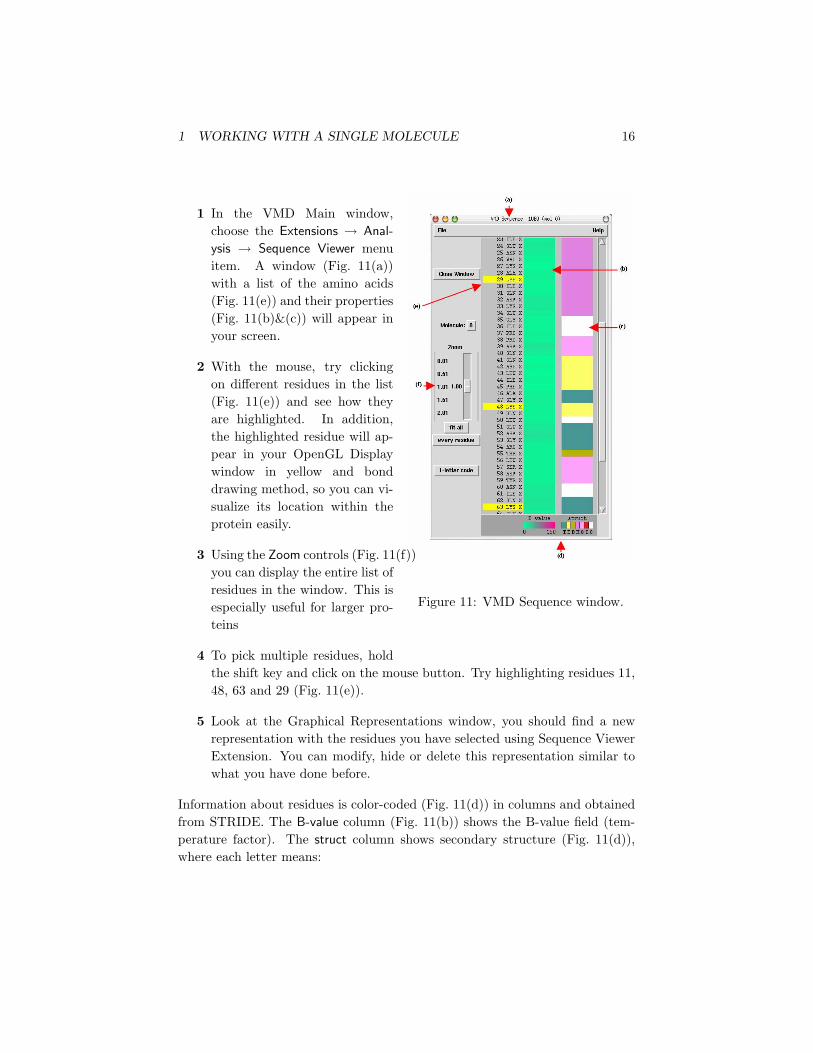
7 Hide the current representation showing all frames, and display only thewater representation by double-clicking on it. Change the text in theSelected Atoms from water to water and within 3 of protein and hitenter. This will show all water atoms within 3 A of the protein.
8 Play the trajectory. Although the displayed water atoms may be nearthe protein for a little while, they soon wander off, and are still showndespite no longer meeting the selection criteria. The Update Selection
Every Frame option in the Trajectory tab of the Graphical Representations
2 TRAJECTORIES AND MOVIE MAKING 29
window remedies this. If the option box is checked, the selection is updatedevery frame. See Fig. 19.
9 Quit VMD.
Figure 19: Water within 3 A of the protein, shown for a selection that is notupdated and for the one that is updated each frame. The snapshots shown are(from left to right) for frames 0, 17, and 99.
2.4 The Basics of Move Making in VMD
We will now learn how to make a basic movie.
1 Start a new VMD session. Repeat steps 1-5 in Section 2.1 to load theubiquitin trajectory into VMD and display the protein in a secondarystructure representation.
2 To make movies, we will use the VMD Movie Maker plugin. In the VMDMain window, go to menu item Extensions → Visualization → Movie Maker.The VMD Movie Generator window will appear (Fig. 20).

2 TRAJECTORIES AND MOVIE MAKING 30
2.4.1 Making single-frame movies
3 First, let us look at some of the options for making a movie. Click onthe Movie Settings menu in the VMD Movie Generator window. You cansee that in addition to a trajectory movie, Movie Maker can also make amovie by rotating the view point of a single frame. In the Renderer menu,one can choose the type of renderer for making the movie. We will usethe default option, Snapshot. One can also choose the output file formatfor the movie in menu item Format.
Movie rendering. While renderers other than Snapshot, such as
Tachyon, generally provide more visually appealing images, they also
require longer time for rendering. The rendering time is also affected
by the size of the OpenGL window, since it takes more computing
time to render a larger image. Likewise, the size of the movie file is
determined by the size (resolution) of that window.
4 We will first make a movie of just one frame of the trajectory. For thatpurpose, select Rock and Roll option in the Movie Settings menu in theVMD Movie Generator window. Set the working directory to any conve-nient directory of your choice, give your movie a name, and click Make
Movie.
5 Once rendering is finished, open and view the movie with your favoriteapplication. This movie setting is good for showing one side of your systemprimarily.
Software requirements. If you cannot successfully make
movies with VMD, it’s possible that you’re missing some
softwares required for generating movies. All the re-
quired softwares are freely available, and to find what soft-
ware you need, please see the VMD Movie Plugin page at
http://www.ks.uiuc.edu/Research/vmd/plugins/vmdmovie/.
2.4.2 Making trajectory movies
6 Now we will make a movie of the trajectory. In the VMD Movie Generatorwindow, select Movie Settings → Trajectory, give this one a different name,and click Make Movie. Note that the length of the movie is automaticallyset 24 frames per second. For a trajectory, duration of the movie can bedecreased, but cannot be increased.
7 Try out different options in the VMD Movie Generator window. Once youare done, quit VMD.

2 TRAJECTORIES AND MOVIE MAKING 31
Figure 20: The VMD Movie Generator window.

3 SCRIPTING IN VMD 32
3 Scripting in VMD
VMD provides embedded scripting languages (Python and Tcl) for the purposeof user extensibility. In this section we will discuss the basic features of the Tclscripting interface in VMD. You will see that everything you can do in VMDinteractively can also be done with Tcl commands and scripts, and how theextensive list of Tcl text commands can help you investigate molecule propertiesand perform analysis.
The Tcl/Tk scripting language. Tcl is a rich language that con-
tains many features and commands, in addition to the typical con-
ditional and looping expressions. Tk is an extension to Tcl that per-
mits the writing of graphical user interfaces with windows and but-
tons, etc. More information and documentations about the Tcl/Tk
language can be found at http://www.tcl.tk/doc.
3.1 The Basics of Tcl Scripting
To execute Tcl commands, you will be using a convenient text console calledTk Console.
1 Start a new VMD session. In the VMD Main menu select Extensions →Tk Console to open the VMD TkConsole window (Fig. 21). You can nowstart entering Tcl/Tk commands here.
Figure 21: The VMD Tk Console window.
Let’s start with the very basics of Tcl/Tk. Here are Tcl’s set and puts com-mands:
set variable value – sets the value of variableputs $variable – prints out the value of variable

3 SCRIPTING IN VMD 33
2 Try entering the following commands in the VMD TkConsole window. Re-member to hit enter after each line and take a look at what you get aftereach input.
set x 10
puts "the value of x is:$x"
set text "some text"
puts "the value of text is:$text."
As you can see, $variable refers to the value of variable.Here is a command that performs mathematical operations:
expr expression – evaluates a mathematical expression
3 Try the expr command by entering the following lines in the VMD Tk-
Console window:expr 3 - 8
set x 10
expr - 3 * $x
One of the most important aspects of Tcl is that you can embed Tcl commandsinto others by using brackets. A bracketed expression will automatically be sub-stituted by the return value of the expression inside the brackets:
[expr.] – represents the result of the expression inside the brackets
4 Create some commands using brackets and test them. Try entering thefollowing example in the VMD TkConsole window:
set result [ expr -3 * $x ]
puts $result
Often, one needs to execute a block of codes for many times. For this purpose,Tcl provides an iterated loop similar to the for loop in C. The for commandin Tcl requires four arguments: an initialization, a test, an increment, and theblock of code to evaluate. The syntax of the for command is:
for {initialization} {test} {increment} {commands}
5 Now let’s calculate the values of −3 ∗ x for integers x from 0 to 10 andoutput the results into a file named myoutput.dat. Please also pay atten-tion the way of writing the output to a file on disk.

3 SCRIPTING IN VMD 34
set file [open "myoutput.dat" w]
for {set x 0} {$x <= 10} {incr x} {puts $file [ expr -3 * $x ]
}close $file
6 Take a look at the output file myoutput.dat, either by a text editor ofyour choice, or the command less in a terminal window on a Mac orLinux Machine.
3.2 VMD scripting
Anything that can be done in the VMD graphical interface can be done withtext commands. This allows scripts to be written that can automatically loadmolecules, create representations, analyze data, make movies, etc. Here, wewill go through some simple examples of what can be done using the scriptinginterface in VMD.
3.2.1 Loading molecules with text commands
1 In the VMD TkConsole window, type the command mol new 1ubq.pdb
and hit enter. As you can see, this command performs the same function asdescribed at the beginning of Section 1.1, namely, loading a new moleculewith file name 1ubq.pdb.
Navigating directories in TkConsole. If you see the
error message Unable to load file ’1ubq.pdb’ using file
type ’pdb’, you might not be in the vmd-tutorial-files di-
rectory. You can use the standard Unix commands in the VMD Tk-
Console window to move to the correct directory where 1ubq.pdb is
located.
When you open VMD, by default a vmd console window appears. The vmdconsole window tells you what’s going on within the VMD session that you areworking on.
2 Take a look at the vmd console window (Fig. 22). It should tell youa molecule has been loaded, as well as some of its basic properties likenumber of atoms, bonds, residues and etc. The Tcl commands that youenter in the VMD TkConsole window can also be entered in the vmdconsole window. If you are using a Mac, your vmd console window is theterminal window that shows up when you open VMD.

3 SCRIPTING IN VMD 35
Figure 22: The VMD Console window.
3.2.2 The atomselect command
Many times you might want to perform operations on only a specific part amolecule. For this purpose, VMD’s atomselect command is very useful.
atomselect molid selection – creates a new atom selection
This command allows you to select a specific part of a molecule. The firstargument to atomselect is the molecule ID (shown to the very left of theVMD Main window), the second argument is a textual atom selection like whatyou have been using to describe graphical representations in Section 1.3. Theselection returned by atomselect is itself a command which you will learn touse.
3 Type set crystal [atomselect top "all"] in the Tk Console window.This creates a selection, crystal, that contains all the atoms in themolecule and assigns it to the variable crystal. Instead of a moleculeID (which is a number), we have used the shortcut “top” to refer to thetop molecule. A top molecules means that it is the target for script-ing commands. This concept is particularly important when multiplemolecules are loaded at the same time (see Section 4 for dealing withmultiple molecules in VMD).
The result of atomselect is a function. Thus, $crystal is now a function thatperforms actions on the contents of the “all” selection.
3.2.3 Obtaining and changing molecule properties with text com-mands
After you have defined an atom selection, you have many commands that youcan use to operate on it. For example, you can use commands to learn aboutthe properties (number of atoms, coordinates, total charge, etc) of your atom
3 SCRIPTING IN VMD 36
selection. You can also use commands to change its coordinates and otherproperties. See VMD User’s Guide2 for an extensive list of commands.
4 Type $crystal num in the Tk Console window. Passing num to an atomselection returns the number of atoms in that selection. Check that thisnumber matches the number of atoms for your molecule displayed in theVMD Main window.
5 We can also use commands to move our molecule on the screen. You canuse these commands to change atom coordinates.
$crystal moveby {10 0 0}$crystal move [transaxis x 40 deg]
The following examples will show you how to edit atomic properties usingVMD’s atomselect command.
6 Open the Graphical Representation window by selecting Graphics → Repre-
sentations. . . in the VMD Main window. Type in protein as the atomselection, change its Coloring Method to Beta and its Drawing Method toVDW. Your molecule should now appear as a mostly red and blue assemblyof spheres.
The PDB B-factor field. The “B” field of a PDB file typically
stores the “temperature factor” for a crystal structure and is read
into VMD’s “Beta” field. Since we are not currently interested in
this information, we can recycle this field to store our own numerical
values. VMD has a “Beta” coloring method, which colors atoms
according to their B-factors. By replacing the Beta values for various
atoms, you can control the color in which they are drawn. This is
very useful when you want to show a property of the system that
you have computed.
7 Return to the Tk Console window, and type $crystal set beta 0. Thisresets the “beta” field (which is displayed) to zero for all atoms. As youdo this, you should observe that the atoms in your OpenGL window willsuddenly change to a uniform color (since they all have the same betavalues now).
Examples of atomic properties. You can obtain and set many
atomic properties using atom selections, including segment, chain,
residue, atom name, position (x, y and z), charge, mass, occupancy
and radius, just to name a few.
2The web version of VMD User’s Guide can be found athttp://www.ks.uiuc.edu/Research/vmd/current/ug/.

3 SCRIPTING IN VMD 37
Atom selections are just references to the atoms in the original molecule. Whenyou change a property (e.g. beta value) of some atoms through a selection, thatchange is reflected in all the other selections that contain those atoms.
8 In the Tk Console window, type set sel [atomselect top "hydrophobic"].This creates a selection, sel, that contains all the atoms in the hydropho-bic residues.
9 Let’s label all hydrophobic atoms by setting their beta values to 1. Youprobably know how to do this by now: type $sel set beta 1 in the Tk
Console window. If the colors in the OpenGL Display do not get updated,go to the Graphical Representations window and click on the Apply buttonat the bottom.
10 You will now change a physical property of the atoms to further illus-trate the distribution of hydrophobic residues. In the Tk Console windowtype $crystal set radius 1.0 to make all the atoms smaller and easierto see through, and then $sel set radius 1.5 to make atoms in thehydrophobic residues larger. The radius field affects the way that somerepresentations (e.g., VDW, CPK) are drawn.
You have now created a visual state that clearly distinguishes which parts ofthe protein are hydrophobic and which are hydrophilic. If you have followed theinstructions correctly, your protein should resemble Fig. 23.
Figure 23: Ubiquitin in the VDW representation, colored according to the hy-drophobicity of its residues.

3 SCRIPTING IN VMD 38
Identifying hydrophobic residues. Many times in studies of pro-
teins it is important to identify the locations of the hydrophobic
residues, as they often have a functional implication. The method
you have just learned is useful in this task. For example, you can
see easily that in ubiquitin, the hydrophobic residues are almost ex-
clusively contained in the inner core of the protein. This is a typical
feature for small water-soluble proteins. As the protein folds, the
hydrophilic residues will have a tendency to stay at the water inter-
face, while the hydrophobic residues are pushed together and play
a structural role. This helps the protein achieve proper folding and
increases its stability.
Atom selections are useful not only for setting atomic data, but also for gettingatomic information. Let’s say that you wish to communicate which residues arehydrophobic, all you need to do is to create a hydrophobic selection and use getcommand.
11 Try to use get command with your sel atom selection to obtain the namesof hydrophobic residues:
$sel get resname
But there is a problem! Each residue contains many atoms, resulting in multiplerepeated entries. Can you think of a way to circumvent this? We know thateach amino acid has the same backbone atoms. If you pick only one of theseatoms per residue, each residue will be present only once in your selection.
12 Let’s try this solution. Each residue has one and only one α-carbon(name CA = alpha), so type the following in the Tk Console window:
set sel [atomselect top "hydrophobic and alpha"]
$sel get resname
This should give you the list of hydrophobic residues.
13 You can also get multiple properties simultaneously. Try the following:
$sel get resid
$sel get {resname resid}$sel get {x y z}
If you want to obtain some of the structural properties, e.g., the geometric centeror the size of a selection, the command measure can do the job easily.
14 Let’s try using measure with the sel selection:
measure center $sel
measure minmax $sel

3 SCRIPTING IN VMD 39
The first command above returns the geometric center of atoms in sel. And thesecond command returns two vectors, the first containing the minimum x, y, andz coordinates of all atoms in sel, and the second containing the correspondingmaxima.
15 Once you are done with a selection, it is always a good ideal to delete itto save memory:
$sel delete
3.2.4 Sourcing scripts
We have learned many useful commands in VMD. When performing a task thatrequires many lines of commands, instead of typing each line in the Tk Console
window, it is usually more convenient to write all the lines into a script fileand load it in VMD. This is very easy to do. Just use any text editor to writeyour script file, and in a VMD session, use the command source filename toexecute the file. In the vmd-tutorial-file, you will find a simple script filebeta.tcl, which we will execute in VMD as an example. The script beta.tclsets the colors of residues LYS and GLY to a different color from the rest of theprotein by assigning them a different beta value, a trick you have also learnedin Section 3.2.3.
16 In the Tk Console window, type source beta.tcl and observe the colorchange. You should see that the protein is mostly a collection of redspheres, with some residues shown in blue. The blue residues are the LYSand GLY residues in the ubiquitin.
17 Let’s take a quick look at the beta.tcl. Use any text editor of yourchoice, open the file beta.tcl. You can see that there are six lines inthis file, and each line represents a Tcl command line that you have usedbefore. Close the text editor when you are done.
A vmd saved state is a script file. The .vmd file you saved in
Section 1.5 is actually a series of commands. You are encouraged
to take a look at that file using a text editor. Hopefully, by the end
of this section, you’ll understand many of those commands. In fact,
you can execute the file at Tk Console the same way as you execute
other script files, i.e., by typing source myfirststate.vmd in the
Tk Console window.
3 SCRIPTING IN VMD 40
The logfile console command. Many times you might want to
look up the command for an interactive VMD feature. You can ei-
ther find it in the VMD User’s Guide3, or use the logfile console
command. Try typing logfile console in your Tk Console win-
dow. This creates a logfile for all your actions in VMD and writes
them in the Tk Console window as command lines. If you exe-
cute those command lines you can repeat the exact same actions
you have performed interactively. To turn off logfile, type logfile
off.
vmdrc. Many times, you would like to automatically load certain
scripts or packages upon starting VMD. VMD has a preferences file
.vmdrc in your home directory (Windows uses the file vmd.rc) for
this purpose. You can also change the default behavior of VMD
here (e.g., change the background color) and add atom selection
macros. VMD will look for this file upon startup and will recognize
all your scripts, macros, etc.. For more information on the VMD
startup files, refer to the VMD user’s guide.
3.3 Drawing shapes
VMD offers a way to display user-defined objects built from graphics primi-tives such as points, lines, cylinders, cones, spheres, triangles, and text. Thecommand that can realize those functions is graphics, the syntax of which is
graphics molid command
Where molid is a valid molecule ID and command is one of the commands shownbelow. Let’s try drawing some shapes with the following examples.
1 Hide all representations in the Graphical Representations window.
2 Let’s draw a point. Type the following command in your Tk Console
window:
graphics top point {0 0 10}Somewhere in your OpenGL window there should be a small dot.
3 Let’s draw a line. Type the following command in your Tk Console win-dow:
graphics top line {-10 0 0} {0 0 0} width 5 style solid
This will give you a solid line.3http://www.ks.uiuc.edu/Research/vmd/current/ug/

3 SCRIPTING IN VMD 41
4 You can also draw a dashed line:
graphics top line {10 0 0} {0 0 0} width 5 style dashed
5 All the objects drawn so far are all in blue. You can change the colorof the next graphics object by using the command graphics top color
colorid. The colorid for each color can be found in Graphics → Colors...
menu in VMD Main window. For example, the color for orange is “3”.Type graphics top color 3 in the Tk Console window, and the nextobject you draw will appear in orange.
6 Try the following commands to draw more shapes:
graphics top cylinder {15 0 0} {15 0 10} radius 10 resolution 60 filled no
graphics top cylinder {0 0 0} {-15 0 10} radius 5 resolution 60 filled yes
graphics top cone {40 0 0} {40 0 10} radius 10 resolution 60
graphics top sphere {65 0 5} radius 10 resolution 80
graphics top triangle {80 0 0} {85 0 10} {90 0 0}graphics top text {40 0 20} "my drawing objects"
7 On your OpenGL window, there are a lot of objects now. To find the listof objects you’ve drawn, use the command graphics top list. You’llget a list of numbers, standing for the ID of each object.
8 The detailed information about each object can be obtained by typinggraphics top info ID. For example, type graphics top info 0 to seethe information on the point you drew.
9 You can also delete some of the unwanted objects using the commandgraphics top delete ID .
10 Using these basic shape-drawing commands, you can create geometric ob-jects, as well as texts, to be displayed in your OpenGL window. Whenyou render an image (as discussed in Section 1.6.5), these objects will beincluded in the resulting image file. You can hence use geometric objectsand texts to point or label interesting features in your molecule. Whenyou are done, quit VMD.

4 WORKING WITH MULTIPLE MOLECULES 42
4 Working with Multiple Molecules
In this section you will learn to deal with multiple molecules within one VMDsession. We will use the water transporting channel protein, aquaporin, as anexample.
4.1 Main Menu Molecule List Browser
Aquaporins are membrane channel proteins found in a wide range of species,from bacteria to plants to human. They facilitate water transport across thecell membrane, and play an important role in the control of cell volume andtranscellular water traffic. Many aquaporin protein structures are available inthe Protein Data Bank, including the human aquaporin (PDB code 1FQY;Murata et al., Nature, 407:599, 2000) and E. coli aquaporin (PDB code 1RC2;Savage et al., PLoS Biology, 1:E72, 2003). To practice dealing with multipleproteins with VMD, let’s load both aquaporin structures.
4.1.1 Loading multiple molecules
1 Start a new VMD session. In the VMD Main window, choose File → New
Molecule.... The Molecule File Browser window should appear on yourscreen.
2 Use the Browse... button to find the file 1fqy.pdb in vmd-tutorial-files
in the tutorial directory. When you select the file, you will be back inthe Molecule File Browser window. Press the Load button to load themolecule. The coordinate file of human aquaporin AQP1 should now beloaded and can be seen in the OpenGL window.
3 The Molecule File Browser window should still be open; if not openit through File → New Molecule... again. Make sure you choose New
Molecule in the Load files for: pull-down menu on the top. Use theBrowse... button to find the file 1rc2.pdb in vmd-tutorial-files direc-tory and press Load. Close the Molecule File Browser window.
You have just loaded a second molecule; any number of molecules may be loadedand displayed in VMD simultaneously by repeating the previous step. VMD canload as many molecules as the memory of your computer allows.Take a look at your VMD Main window, which should look like Fig. 24. Withinthe VMD Main menu you can find the Molecule List Browser (circled in Fig. 24),which shows the global status of the loaded molecules. The Molecule ListBrowser displays information about each molecule, including Molecule ID (ID),the four Molecule Status Flags (T, A, D, and F, which stand for Top, Active,Drawn, and Fixed), name of the molecule (Molecule), number of atoms in the

4 WORKING WITH MULTIPLE MOLECULES 43
molecule (Atoms), number of frames loaded in the molecule (Frames), and thevolumetric data loaded (Vol).
Figure 24: The Molecule List Browser.
4.1.2 Changing molecule names
Let’s first start with the Molecule column. By default the Molecule columndisplays file names of the molecules loaded in VMD, but you can change themolecule names to recognize them more easily.
4 In the VMD Main menu, double-click on 1fqy.pdb in the Molecule col-umn. A window will pop up with the message “Enter a new name for
molecule 0:” (Fig. 24a). Type in “human aquaporin”, and click OK (orpress enter). In the VMD Main menu, the first molecule now has thename “human aquaporin”.
5 Repeat the previous step for the E. coli aquaporin by double-clicking the1rc2.pdb molecule name, and changing it to “E. coli aquaporin” in thepop-up window. Your VMD Main window should now look like Fig. 25b.
Figure 25: Changing molecule names.

4 WORKING WITH MULTIPLE MOLECULES 44
4.1.3 Drawing different representations for different molecules
Before we continue exploring other features in the Molecule List Browser, takea look at your OpenGL Display window. You have two aquaporin structures,but since they are both shown in the same default representation, it is diffi-cult to distinguish them. To tell them apart, you can assign them differentrepresentations.
6 Open the Graphical Representations window via Graphics → Represen-
tations... from the VMD Main menu. Make sure 0:human aquaporin isselected in the Selected Molecule pull-down menu on top. Select New Car-
toon for Drawing method, and ColorID → 1 red for Coloring Method.
7 In the Graphical Representations window, select 1:E. coli aquaporin in theSelected Molecule pull-down menu on top. Select New Cartoon for Drawing
method, and ColorID → 4 yellow for Coloring Method. Close the GraphicalRepresentations window.
Now your OpenGL Display window should show a human aquaporin colored inred and an E. coli aquaporin colored in yellow (Fig. 26).
Figure 26: The two aquaporins drawn in different representations.
4.1.4 Molecule Status Flags
In your OpenGL Display window, try moving the aquaporins around with yourmouse in different mouse modes (rotating, scaling, and translating). You can

4 WORKING WITH MULTIPLE MOLECULES 45
see that both aquaporins move together. You can fix any molecule by double-clicking the F (fixed) flag in the Molecule List Browser on the left of the moleculename.
8 In the Molecule List Browser, double-click on the F flag on the left ofhuman aquaporin to fix the human aquaporin molecule. Return to theOpenGL Display window and toggle your mouse around. You can see thatonly the yellow E. coli aquaporin moves. Double-click on the F flag forhuman aquaporin again to release it.
One thing to notice about the F flag is that, although it may seem that onemolecule has been moved relative to another when one of the molecules is fixed,the difference is only apparent. The internal coordinates of molecules are notchanged by the rotation, translation and scaling motions. To change the co-ordinates of atoms in a molecule you need to use the text command interface(discussed in Section 3.2.3), and by using the atom move picking modes (bychoosing Mouse → Move in the VMD Main menu).Other features in the Molecule List Browser includes the Molecule ID (ID),Top (T), Active (A), and Drawn (D). Molecule ID is a number (starting from0) assigned to each molecule when it’s loaded into VMD, and is how VMDrecognizes each molecule internally. You also refer to molecules by their MoleculeIDs in text command interface. Top flag (T) indicates the default molecule inVMD operations, for example when resetting the VMD OpenGL view and whenplaying molecule trajectories. There can be only one top molecule at a time.Active flag (A) indicates if the trajectory of the given molecule is updated whenusing animation tools described in Section 2. Finally, Drawn flag (D) indicatesif the given molecule is displayed in the OpenGL window. Let’s try out the Topand Drawn flags.
9 Make sure no molecule is fixed. By default the last molecule loaded inthe VMD is the top molecule, so you can check and see that there is aT displayed for the E. coli aquaporin in the VMD Main menu. Resetthe view by pressing “=” in the OpenGL Display window. Note thatthe yellow E. coli aquaporin is now placed in the center of the OpenGLDisplay window.
10 Switch the top molecule by double-clicking on the empty T flag for thehuman aquaporin molecule in the VMD Main menu. A T should appearfor the human aquaporin, while the T for E. coli disappears. Go to theOpenGL Display window and reset the view again. You can see that thistime the red human aquaporin is placed in the center of the OpenGLDisplay window.

4 WORKING WITH MULTIPLE MOLECULES 46
11 In the VMD Main menu, try hiding a molecule by double-clicking on itsD flag. You can display the molecule again by double-clicking its D flagagain.
4.2 Aligning Molecules with the measure fit Command
When you look at your OpenGL Display window, you can see that the twoaquaporins are very similar in structure. But it is difficult to detect their slightstructural differences as the two proteins are placed apart. We will now try outa very useful Tcl command measure fit to align two molecules.
Figure 27: Result of the alignment between the two aquaporins using themeasure fit command.
1 Open the VMD TkConsole window by choosing Extension → TkConsole
from the VMD Main menu, and input the following commands (hit Enterafter each line):
set sel0 [atomselect 0 all]
set sel1 [atomselect 1 all]
set M [measure fit $sel0 $sel1]
$sel0 move $M
measure fit selection1 selection2– measures the transformation matrix that best aligns thecoordinates of selection1 with the coordinates of selection2

4 WORKING WITH MULTIPLE MOLECULES 47
As soon as you enter the last command line, you can see that the two aquaporinsare now overlapping (Fig. 27). The α-helical regions of the aquaporins agreevery well, with bigger deviations in the loop regions. Note the measure fit
command can only work if two molecules have the same number of atoms. Inthis case it’s a pure coincidence that the human aquaporin and E. coli aquaporinPDB files have the same number of atoms. The measure fit command is hencemost useful in aligning the same protein in different conformations or differentframes of a molecular dynamics simulation trajectory. Generally, to comparethe structures of different proteins, one needs to use a different method. A goodtool is the MultiSeq VMD plugin, which we will discuss in the following section.
2 Quit VMD.
5 COMPARING STRUCTURES AND SEQUENCES WITH MULTISEQ 48
5 Comparing Structures and Sequences with Mul-
tiSeq
MultiSeq (Roberts et al., BMC Bioinformatics, 7:382, 2006) is a bioinformaticsanalysis environment developed in the Luthey-Schulten Group at the Universityof Illinois in Urbana-Champaign. MultiSeq allows users to organize, display, andanalyze both sequence and structure data for proteins and nucleic acids4, andhas been incorporated in VMD as a plugin tool starting with VMD version 1.8.5.In this section you will learn how to compare protein structures and sequenceswith the VMD MultiSeq plugin. We will again use the water transportingchannel protein, aquaporin, as an example.
5.1 Structure Alignment with MultiSeq
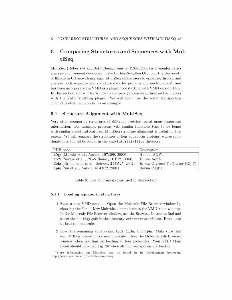
Very often comparing structures of different proteins reveal many importantinformation. For example, proteins with similar functions tend to be foundwith similar structural features. MultiSeq structure alignment is useful for thisreason. We will compare the structures of four aquaporin proteins, whose coor-dinate files can all be found in the vmd-tutorial-files directory.
PDB code Description1fqy (Murata et al., Nature, 407:599, 2000) Human AQP11rc2 (Savage et al., PLoS Biology, 1:E72, 2003) E. coli AqpZ1lda (Tajkhorshid et al., Science, 296:525, 2002) E. coli Glycerol Facilitator (GlpF)1j4n (Sui et al., Nature, 414:872, 2001) Bovine AQP1
Table 8: The four aquaporins used in this section.
5.1.1 Loading aquaporin structures
1 Start a new VMD session. Open the Molecule File Browser window bychoosing the File → New Molecule... menu item in the VMD Main window.In the Molecule File Browser window, use the Browse... button to find andselect the file 1fqy.pdb in the directory vmd-tutorial-files. Press Load
to load the molecule.
2 Load the remaining aquaporins, 1rc2, 1lda, and 1j4n. Make sure thateach PDB is loaded into a new molecule. Close the Molecule File Browserwindow when you finished loading all four molecules. Your VMD Mainmenu should look like Fig. 28 when all four aquaporins are loaded.
4More information on MultiSeq can be found in its development homepagehttp://www.scs.uiuc.edu/ schulten/multiseq

5 COMPARING STRUCTURES AND SEQUENCES WITH MULTISEQ 49
Figure 28: VMD Main menu after loading the four aquaporins.
5.1.2 Aligning the molecules
3 Within the VMD main window, choose the Extensions menu and selectAnalysis → MultiSeq.
The Multiseq window (with window name untitled.multiseq showing on top)should now be open. You may be asked to update some databases in a pop-upwindow if this is the first time you use MultiSeq. If this is the case, simply clickYes and wait for MultiSeq to finish downloading. When MultiSeq starts, yourMultiseq window should look like Fig. 29, with a list of the four aquaporin proteinstructures and a list of two non-protein structures. The non-protein structuresare detergent molecules used in crystallizing the aquaporin proteins, and willnot be needed for structure or sequence alignment. You can tell MultiSeq tothrow away molecules you are not interested in.
Figure 29: The MultiSeq window.
4 In the Multiseq window, select the 1lda X detergent molecule by clicking onit. This will highlight the entire row of 1lda X. Remove it from MultiSeq

5 COMPARING STRUCTURES AND SEQUENCES WITH MULTISEQ 50
by pressing the delete or Backspace key on your keyboard. Do the sameto remove the 1j4n X detergent molecule.
MultiSeq uses the program STAMP (Russell et al., Proteins: Struct., Func.,Gen., 14:309, 1992) to align protein molecules. STAMP (Structural Alignmentof Multiple Proteins) is a tool for aligning protein sequences based on a three-dimensional structure. Its algorithm minimizes the Cα distance between alignedresidues of each molecule by applying globally optimal rigid-body rotations andtranslations. Note that you can only perform alignments on molecules that arestructurally similar; if you try to align proteins that have no common structures,STAMP will have no means of aligning them.
5 In the Multiseq window, select Tool → Stamp Structural Alignment. Thiswill open the Stamp Alignment Options window.
6 In the Stamp Alignment Options window, choose Align the following: All
Structures and go to the bottom of the menu and press OK.
The molecules have been aligned. You can see the alignment both in theOpenGL window and in the MultiSeq window (Fig. 30). Your alignment inOpenGL window will not immediately resemble Fig. 30. When MultiSeq com-pletes an alignment, it creates a new representation for all the aligned proteinin the NewCartoon representation with the same default coloring method andhides all other representations created previously. Let’s give different colors todifferent aquaporins to distinguish them.
Figure 30: The four aquaporins aligned according to their structural similarity.
7 Open your Graphical Representations window, and you should see two rep-resentations for each molecule, one on top created when VMD loaded themolecule (which is now hidden), and one on the bottom created automat-ically by MultiSeq. Select 0:1fqy.pdb in the Selected Molecule pull-down

5 COMPARING STRUCTURES AND SEQUENCES WITH MULTISEQ 51
menu on top and highlight the bottom representation by clicking on it.Change the color for this representation by selecting ColorID → 1 red forColoring Method.
8 In the Graphical Representations window, select 1:1rc2.pdb in the Selected
Molecule pull-down menu on top and highlight the bottom representationby clicking on it. Select ColorID → 4 yellow for Coloring Method.
9 In the Graphical Representations window, select 2:1lda.pdb in the Selected
Molecule pull-down menu on top and highlight the bottom representationby clicking on it. Select ColorID → 11 purple for Coloring Method.
10 In the Graphical Representations window, select 3:1j4n.pdb in the Selected
Molecule pull-down menu on top and highlight the bottom representationby clicking on it. Select ColorID → 12 lime for Coloring Method. Close theGraphical Representations window.
Now your OpenGL window should look similar to Fig. 30, and you can see thatthe alignment was pretty good as the four aquaporin structures are very similar.You can also get more information about the alignment in the MultiSeq windowby highlighting the molecules you wish to compare.
11 In the MultiSeq window, highlight 1fqy by clicking on it. To highlightanother molecule without unhighlighting 1fqy, you need to Ctrl-click (orcommand-click on Mac) on that molecule. Highlight 1rc2 by clicking onit while holding down the Ctrl key on the keyboard (or the command keyon Mac). When both 1fqy and 1rc2 are highlighted, you should see onthe lower left corner in the MultiSeq window a line of text: QH:0.6442,
RMSD:2.3043, Percent Identity:30.28 as shown in Fig. 31. Note, thevalues you obtain might be a little different depending on if your MultiSeqdatabase is updated, but they should be close to the ones in Fig. 31.
The QH value is a metric for structural homology. It’s an adaptation of the Qvalue that measures structural conservation5. Q=1 implies that structures areidentical. When Q has a low score (0.1-0.3), structures are not aligned well,i.e., only a small fraction of the Cα atoms superimpose. Along with RMSD andPercent Identity, these numbers tell you that the 1fqy and 1rc2 structures arepretty well aligned. You can repeat the previous step to compare the alignmentof other molecules. To unselect a highlighted molecule, Ctrl-click on it again(or command-click on Mac).
5Eastwood, M.P., C. Hardin, Z. Luthey-Schulten, and P.G. Wolynes. “Evaluating theprotein structure-prediction schemes using energy landscape theory.” IBM J. Res. Dev. 45:475-497, 2001. URL: http://www.research.ibm.com/journal/rd/453/eastwood.pdf

5 COMPARING STRUCTURES AND SEQUENCES WITH MULTISEQ 52
Figure 31: The QH , RMSD, and Percent Identity values can be used to deter-mine how good an alignment is between two molecules, and how similar theyare in structure and sequence.
5.1.3 Coloring molecules by their structural identity
You can also color the molecules according to the value of Q per residue (Qres)obtained in the alignment. Qres is the contribution from each residue to theoverall Q value of aligned structures.
12 In the MultiSeq window, choose View → Coloring → Qres.
13 Look at the OpenGL window to see the impact this selection has madeon the coloring of the aligned molecules (Fig. 32). The blue areas indicatethat the molecules are structurally conserved at those points. If there is nocorrespondence in structural proximities at these points, the points appearred. As you can see the α-helices that form the pore are well conservedstructurally among the four aquaporins, while there are more structuraldifference in the less functionally relevant loops.
5.2 Sequence Alignment with MultiSeq
Besides studying structural similarities, MultiSeq also allows protein compari-son based on their sequence information. Sequence alignment is often used toidentify conserved residues among similar proteins, as such residues are likelyfunctionally important.

5 COMPARING STRUCTURES AND SEQUENCES WITH MULTISEQ 53
Figure 32: Result of a structural alignment of the four aquaporins, colored byQres.
5.2.1 Aligning molecules and coloring molecules by degree of con-servation
1 In the MultiSeq window, select Tools → ClustalW Sequence Alignment win-dow. In the ClustalW Alignment Options window, make sure the Align All
Sequences option is checked, and go to the bottom of the window andselect OK. Now the four aquaporins have been aligned according to theirsequence using the ClustalW tool (Thompson et al., Nucl. Acids Res.,22:4673, 1994).
2 Let’s color the aligned molecules by their sequence similarity. In the Mul-
tiseq window, choose View → Coloring → Sequence identity. Now eachamino acid is colored according to the degree of conservation within thealignment: blue means highly conserved, whereas red means very low orno conservation. Your MultiSeq window and OpenGL window should nowresemble Fig. 33.
You have now aligned the four aquaporins by their sequence and identified theconserved residues, which tend to locate inside the pore (Fig. 34). Since aqua-porin facilitates water transport across the membrane, these conserved residuesare most likely the ones that carry out this important function.
5.2.2 Importing FASTA files for sequence alignment
Many times the structure of a protein might not be available, but its sequenceis. You can analyze a protein in MultiSeq without its structure by loading itssequence information in the FASTA file format. If you don’t have the FASTAfile of a protein but you have its sequence, you can create a FASTA file easilywith any text editor of your choice.

5 COMPARING STRUCTURES AND SEQUENCES WITH MULTISEQ 54
Figure 33: Result of a sequence alignment of the four aquaporins, colored bysequence identity.
Figure 34: Top view of the aligned aquaporins colored by sequence conservation.The conserved residues locate mostly inside the aquaporin pore.
3 In the vmd-tutorial-files directory, find the provided FASTA sequencefile spinach aqp.fasta and open it with a text editor (Fig. 35a). AFASTA file contains a header that starts with “>”, followed by the nameof the protein. In the next line is the protein sequence in one-letter aminoacid code. You can create FASTA files similarly in this format. When youcreate a FASTA file, remember to save it in plain text, and use .fasta

5 COMPARING STRUCTURES AND SEQUENCES WITH MULTISEQ 55
as the file extension. Close the text editor when you finish examiningspinach aqp.fasta.
Figure 35: The content of spinach aqp.fasta.
4 In the MultiSeq window, select File → Import Data.... Select From File
in the Import Data window, and press the top Browse button to selectthe file spinach aqp.fasta. Press OK on the bottom of the Import Datawindow.
You have now loaded the sequence information of a spinach aquaporin intoMultiSeq (Fig. 35b). You can now preform sequence alignment on the spinachaquaporin protein with other loaded aquaporin molecules. Let’s try a sequencealignment between spinach and human aquaporins.
5 Click on the checkbox on the left of spinach aqp, and click on the check-box on the left of 1fqy.pdb. Open the ClustalW Alignment Optionswindow by selecting Tools → ClustalW Sequence Alignment. Under theMultiple Alignment options on the top, check Align Marked Sequences. Goto the bottom of the window and select OK.
The sequence of spinach aquaporin is now aligned with the sequence of humanaquaporin, and you can check how good the alignment is by obtaining its QH
and Sequence Identity values. If you feel that the two molecules are listed toofar apart in the MultiSeq window, you can move the molecules by draggingthem with your mouse. Also, as you might have noticed, in MultiSeq moleculescan be “Marked” by checking their checkboxes. They can also be “Selected”by highlighting them. You can align only the molecules of your choice by se-lecting Align Marked Sequences or Align Selected Sequences, depending if youhave marked or highlighted your molecules. This option is available for bothstructural alignment and sequence alignment.The structures of spinach aquaporin are actually available (Tornroth-Horsefieldet al., Nature, 439:688, 2006), but now that you have learned how to importFASTA sequence data, you can compare the sequences of proteins even if theirstructures are not yet published.

5 COMPARING STRUCTURES AND SEQUENCES WITH MULTISEQ 56
6 When you finish comparing the sequence of spinach aquaporin with otheraquaporins, delete it by clicking on spinach aqp and press delete orBackspace on your keyboard.
5.3 Phylogenetic Tree
The Phylogenetic Tree feature in MultiSeq elucidates the structure-based and/orsequence-based relationships between different proteins. Structure-based phylo-genetic trees can be constructed according to the RMSD or Q values between themolecules after alignment; sequence-based phylogenetic trees can be constructedaccording to the percent identity or ClustalW values.
The Phylogenetic Tree. A phylogenetic tree is a dendogram, rep-
resenting the succession of biological form by similarity-based clus-
tering. Classical taxonomists use these methods to infer evolution-
ary relationships of multicellular organisms based on morphology.
Molecular evolutionary studies use DNA, RNA, protein sequences or
protein structures to depict the evolutionary relationships of genes
and gene products. In this tutorial we employ QH and RMSD to
depict evolution of protein structure. For a comprehensive expla-
nation of phylogenetic trees, see Inferring Phylogenies by Joseph
Felsenstein6.
1 Align the structures again, by going to the Multiseq window and selectingTools → Stamp Structural Alignment.
2 In the Stamp Structural Alignment window, select All Structures, and keepthe default values for the rest of the parameters. Press the OK button toalign the structures.
3 In the Multiseq program window choose Tools → Phylogenetic Tree. ThePhylogenetic tree window will open.
4 Select Structural tree using QH , and press the OK button. A phylogenetictree based on the QH values will be calculated and drawn as shown inFig. 36. Here you can see the relationship between the four aquaporin,e.g., how the E.Coli AqpZ (1r2c) is related to human AQP1 (1fqy).
5 You can also construct the phylogenetic tree of the four aquaporins basedon their sequence information. Close the Tree Viewer window
6J. Felsenstein Inferring Phylogenies. Sinauer Associates, Inc.: 2004.

5 COMPARING STRUCTURES AND SEQUENCES WITH MULTISEQ 57
Figure 36: a) A structure-based phylogenetic tree generated by QH values. b)A sequence-based phylogenetic tree generated by ClustalW.
6 You need to perform the sequence alignment again for the four aquaporinproteins. In your MultiSeq window, choose Tools → ClustalW Sequence
Alignment, and make sure the Align All Sequences option is checked, andpress Ok.
7 In the Multiseq program window choose Tools → Phylogenetic Tree to openPhylogenetic tree window again.
8 Select Sequence tree using ClustalW, and press the OK button. A phylo-genetic tree based on ClustalW will be calculated and drawn as shown inFig. 36.
9 Quit VMD.

6 DATA ANALYSIS IN VMD 58
6 Data Analysis in VMD
VMD is a powerful tool for analysis of structures and trajectories. Numer-ous tools for analysis are available under the VMD Main menu item Exten-
sions→Analysis. In addition to these built-in tools, VMD users often use custom-written scripts to analyze desired properties of the simulated systems. VMDTcl scripting capabilities are very extensive, and provide boundless opportuni-ties for analysis. In this following section, we will learn how to use built-in VMDfeatures for standard analysis, as well as consider a simple example of scripting.
6.1 Labels
Labels can be placed in VMD to get information on a particular selection, tobe used during visualization and quantitative analysis. Labels are selected withthe mouse and can be accessed in Graphics → Labels menu. We will cover labelsthat can be placed on atoms and bonds, although angle and dihedral labelingare also available. In this context, labels for “bonds” or “angles” actually meandistances between two atoms or angles between three atoms; the atoms do nothave to be physically connected by bonds in the molecule.
1 Start a new VMD session. Load the ubiquitin trajectory into VMD (usingthe files ubiquitin.psf and pulling.dcd). For graphical representation,display protein only, using New Cartoon for drawing method and Structure
for coloring method. If you need help, check Section 2.1, steps 1-5.
2 Choose the Mouse → Labels → Atoms menu item from the VMD Mainmenu. The mouse is now set to the mode for displaying atom labels. Youcan click on any atom on your molecule and a label will be placed for thisatom. Clicking again on it will erase the label.
3 We will now try the same for bonds. Choose the Mouse → Label → Bonds
menu item from the VMD Main menu. This selects the “Display Labelfor Bond” mode.
We will consider the distance between the α carbon of Lysine 48 and of theC terminus. In the pulling simulation, the former is kept fixed, and the latteris pulled at a constant force of 500 pN. In reality, polyubiquitin chains can belinked by a connection between the C terminus of one ubiquitin molecule andthe Lysine 48 of the next. The simulation then mimics the effect of pulling onthe C terminus with this kind of linkage.
4 We will make a VDW representation for the α carbons of Lysine 48 andof the C terminus. To find out the index of these atoms, make a selectionincluding these two atoms, by typing in the Tk Console window (to open

6 DATA ANALYSIS IN VMD 59
the Tk Console window, select Extensions → Tk Console in the VMD Mainmenu.):set sel [atomselect top "resid 48 76 and name CA"].
5 Get the indices by typing the following line in the Tk Console window:$sel get index
This command should give the indices 770 1242.
PDB and VMD atom numbering. Note that the atom number of
these atoms in the pdb file is 771 and 1243. VMD starts counting
the index from zero, so the text in the Representation should be
the numbers that VMD understands. This is only the case for index,
since VMD does not read them from the PDB file. Other keywords,
such as residue, are consistent with the PDB file.
6 In the Graphical Representations window, create a representation for theselection index 770 1242, with VDW as drawing method.
7 Now that you can see the two α carbons, choose the Mouse→ Label→ Bonds
menu item from the VMD Main menu. Click on each atom one after theother. You should get a line connecting the two atoms (Fig. 37). Thenumber appearing next to the line is the distance between the two atomsin Angstroms. Note that the appearance of the line (its color), as wellas appearance of essentially all other objects in VMD, can be changed inGraphics → Colors in the VMD Main menu.
Labels. The shortcut keys for labels are 1: Atoms and 2: Bonds.
You can use these instead of the Mouse menu. Be sure the Open
GL Display window is active when using these shortcuts.
8 The value of the distance displayed corresponds to the current frame. Tryplaying the trajectory - you will see that the label is modified automaticallyas the distance between the atoms changes.
9 The labels can be used not only for display, but also for obtaining quan-titative information. In VMD Main menu, select Graphics → Labels. Onthe top left-hand side of the window, there is a pull-down menu where youcan choose the type of label (Atoms, Bonds, Angles, Dihedrals). For now,keep it in Atoms. You can see the list of atoms for which you have madea label.
10 Click on one of the atoms. You can see all the information of the atomdisplayed on the bottom half of the Labels window. This informationis useful to make selections; it corresponds to the current frame, and isupdated as the frame is changed.

6 DATA ANALYSIS IN VMD 60
Figure 37: Labels in VMD. Label control is available in the Graphics → Labelsmenu item, using which, one can, e.g., plot the labeled distance as a function oftime.
11 You can also delete, hide, or show the atom label by clicking on the cor-responding button on the top of the Labels window.
12 Now, in the Labels window, choose the label type Bonds, and select the“bond” (distance) you labeled (Fig. 37). The information given corre-sponds to only the first atom in the bond, but the number in the Value
field corresponds to the length of the bond in Angstroms.
13 Click on the Graph tab. Select the bond you labeled between atoms 770and 1242. Click on the Graph button. This will create a plot of thedistance between these two atoms over time (Fig. 37). You can also savethis data to a file by clicking on the Save button, and then use an externalplotting program to visualize the data.
14 Quit VMD.
6.2 Example of a built-in analysis tool: the RMSD Tra-
jectory Tool
The built-in analysis tools in VMD are available under the menu item Exten-
sions →Analysis. These tools each features a GUI window that allow one toenter parameters and customize the quantities analyzed. In addition, all toolscan be invoked in a scripting mode, using the TkConsole window. We will learnhow to work with one of the most frequently used tools, the RMSD Trajectory
Tool.

6 DATA ANALYSIS IN VMD 61
Root Mean Square Deviation. The Root Mean Squared Deviation
(RMSD) is defined as :
RMSD =
s PNatomsi=1 (ri(t1)− ri(t2))2
Natoms(1)
where Natoms is the number of atoms whose positions are being
compared, and ri(t) is the position of atom i at time t.
In this example, we will analyze RMSD for two trajectories for the samesystem, ubiquitin.psf. One of them is the already familiar pulling trajectory,pulling.dcd, and the other is the trajectory of a simulation in which no forcewas applied to the protein, equilibration.dcd.
1 Start a new VMD session. Load the ubiquitin equilibration trajectory intoVMD (using the files ubiquitin.psf and equilibration.dcd).
2 Choose Extensions → Analysis → RMSD Trajectory Tool in the VMD Mainwindow (Fig. 38). The RMSD Trajectory Tool window will show up.
3 In the RMSD Trajectory Tool window, you can see many customizationscan be made. For the default values, the molecule to be analyzed isubiquitin.psf (the only one loaded). The selection for which RMSDwill be computed is all of the protein atoms, excluding hydrogens (sincethenoh checkbox is on). The RMSD will be calculated for each frame (timet1 in Eq. 1) with the reference to frame 0 (time t2 in Eq. 1). Make surethe Plot checkbox is selected.
4 Click the Align button. This will align each frame of the trajectory withrespect to the reference frame (in this case, frame 0) to minimize RMSD,by applying only rigid-body translations and rotations. This step is notnecessary, but is desirable in most cases, because we are interested onlyin RMSD that arises from the fluctuations of the structure and not fromthe displacements and rotations of the molecule as a whole. The result ofthe alignment can be seen in the OpenGL display.
5 Now, click the RMSD button in the RMSD Trajectory Tool window. Theprotein RMSD (in Angstroms) vs. frame number is displayed in a plot(Fig. 38).

6 DATA ANALYSIS IN VMD 62
Figure 38: RSMD Trajectory Tool. The RMSD is plotted for the equilibrationof ubiquitin.
RMSD plot. Over the several initial frames, RMSD= 0 because
positions of the protein atoms are fixed during that time in the
simulation, to allow water molecules around the protein to adjust to
the protein surface. After that, the protein is released, and RMSD
grows quickly up to around 1.5 A. At that point, RMSD levels off
and remains at ∼1.5 A further on. This is a typical behavior for
MD simulations. Leveling of the RMSD means that the protein
has relaxed from its initial crystal structure (which is affected by
crystal packing and usually misses some atoms, e.g., hydrogens) to
a more stable one. Production MD simulations are usually preceded
by such equilibration runs, where the protein is allowed to relax; the
process is monitored by checking RMSD vs. time, and equilibration
is assumed to be sufficient when RMSD levels off. The RMSD
of 1.5 A is quite a good value, totally acceptable for most protein
simulations. Usually, the deviations from the crystal structure in
a simulation are due to the thermal motion and to the relaxation
process mentioned; imperfections of the simulation force-fields can
contribute as well.
6 We will now work with the other trajectory. Load the pulling trajectoryinto VMD using the files ubiquitin.psf and pulling.dcd. Make sureyou load ubiquitin.psf as a new molecule. You can change the namesof the molecules by double-clicking on them in the VMD Main menu (see

6 DATA ANALYSIS IN VMD 63
Section 4.1.2).
7 In the RMSD Trajectory Tool window, hit the button Add all to updatethe list of molecules.
8 Click the Align button, and then click RMSD. The new graph (Fig. 39)displays two RMSD plots vs. time, one for the equilibration trajectory,and the other for the pulling trajectory. The pulling RMSD does not leveloff and is much higher than the equilibration RMSD, since the protein isstretched in the simulation.
9 Quit VMD.
Figure 39: RMSD vs. time for the equilibration (blue) and pulling (red) trajec-tories of ubiquitin.
6.3 Example of an analysis script
In many cases, one requires special types of trajectory analysis that are tailoredfor certain needs. The Tcl scripting in VMD provides opportunities for suchcustom tasks. Users commonly write their own scripts to analyze the features ofinterest, and a very extensive library of VMD scripts, contributed by many users,is available online, at http://www.ks.uiuc.edu/Research/vmd/script library/.

6 DATA ANALYSIS IN VMD 64
We will investigate a very simple exemplary script, distance.tcl, which com-putes the distance between two atom selections vs. time and also distributionof the distance.
1 Start a new VMD session. Load the ubiquitin equilibration trajectory(files ubiquitin.psf and equilibration.dcd).
2 Open the TkConsole window by selecting Extensions → Tk Console in theVMD Main menu.
3 In the the TkConsole window, load the script into VMD by typing: sourcedistance.tcl (make sure that the file distance.tcl is in the currentfolder). This will load the procedure defined in distance.tcl into theVMD.
4 One can now invoke the procedure by typing distance in the the TkCon-sole window. In fact, the correct usage isdistance seltext1 seltext2 N d f r out f d out
where seltext1 and seltext2 are the selection texts for the groups ofatoms between which the distance is measured, N d is the number of binsfor the distribution, and f r out and f d out are the file names to wherethe output distance vs. time and distance distribution will be written.
5 Open the script file distance.tcl with a text editor. You can see thatthe script does the following:
• Choose atom selectionsset sel1 [atomselect top "$seltext1"]
set sel2 [atomselect top "$seltext2"]
• Get the number of frames in the trajectory and assign this value tothe variable nf
set nf [molinfo top get numframes]
• Open file specified by the variable f r out
set outfile [open $f r out w]
• Loop over all framesfor {set i 0} {$i < $nf} {incr i} {
• Write out the frame number and update the selections to the currentframe
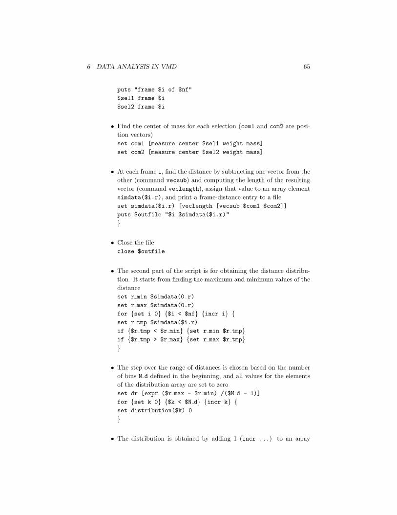
6 DATA ANALYSIS IN VMD 65
puts "frame $i of $nf"
$sel1 frame $i
$sel2 frame $i
• Find the center of mass for each selection (com1 and com2 are posi-tion vectors)set com1 [measure center $sel1 weight mass]
set com2 [measure center $sel2 weight mass]
• At each frame i, find the distance by subtracting one vector from theother (command vecsub) and computing the length of the resultingvector (command veclength), assign that value to an array elementsimdata($i.r), and print a frame-distance entry to a fileset simdata($i.r) [veclength [vecsub $com1 $com2]]
puts $outfile "$i $simdata($i.r)"
}
• Close the fileclose $outfile
• The second part of the script is for obtaining the distance distribu-tion. It starts from finding the maximum and minimum values of thedistanceset r min $simdata(0.r)
set r max $simdata(0.r)
for {set i 0} {$i < $nf} {incr i} {set r tmp $simdata($i.r)
if {$r tmp < $r min} {set r min $r tmp}if {$r tmp > $r max} {set r max $r tmp}}
• The step over the range of distances is chosen based on the numberof bins N d defined in the beginning, and all values for the elementsof the distribution array are set to zeroset dr [expr ($r max - $r min) /($N d - 1)]
for {set k 0} {$k < $N d} {incr k} {set distribution($k) 0
}
• The distribution is obtained by adding 1 (incr ...) to an array

6 DATA ANALYSIS IN VMD 66
element every time the distance is within the respective binfor {set i 0} {$i < $nf} {incr i} {set k [expr int(($simdata($i.r) - $r min) / $dr)]
incr distribution($k)
}
• Write out the file with the distributionset outfile [open $f d out w]
for {set k 0} {$k < $N d} {incr k} {puts $outfile "[expr $r min + $k $dr] $distribution($k)"
}close $outfile
6 Now run the script by typing in the TkConsole windowdistance "protein" "protein and resid 76" 10 res76-r.dat res76-d.dat
This will compute the distance between the center of the protein and cen-ter of the terminal residue 76, and write the distance vs. time and itsdistribution to files res76-r.dat and res76-d.dat.
7 Repeat the same for the protein’s residue 10 by typing in the TkConsolewindowdistance "protein" "protein and resid 10" 10 res10-r.dat res10-d.dat
The data in files produced by the script distance.tcl are in two-columnformat. Compare the outputs for residue 76 and 10 using your favoriteexternal plotting program (Fig. 40).
Residue 76 is at the protein’s C-terminus, which is extended towards the solventand is quite flexible, while residue 10 is at the surface of the globular part ofubiquitin. The difference in their dynamics with respect to the rest of the proteinis immediately obvious when our newly obtained data are plotted (Fig. 40): thedistance of residue 76 from the protein’s center is substantially greater than thatof residue 10, and the distribution of the distance is noticeably wider due to theflexibility of the C-terminus. This is just a simple example of scripting for theanalysis of a trajectory. Similar, but usually much more complex, customizedscripts are routinely employed by VMD users to perform many kinds of analysis.
8 Quit VMD.

6 DATA ANALYSIS IN VMD 67
Figure 40: Distance between a residue and the center of ubiquitin. The distancesanalyzed are those for residue 76 (black) and residue 10 (green).

6 DATA ANALYSIS IN VMD 68
Final Remarks
What we are able to present in this tutorial only showcases a small part ofVMD’s capability. But now that you have learned the basics of VMD, youare ready to explore its many other features most suitable for your research.For this purpose there are many tutorials available that aim to offer a morefocused training, either on a specific tool or on a scientific topic. You can findmany useful documentations, including the comprehensive VMD User’s Guide,in the VMD homepage http://www.ks.uiuc.edu/Research/vmd/. If you haveany question on using VMD, we encourage you to subscribe to the VMD mailinglist http://www.ks.uiuc.edu/Research/vmd/mailing list/.
Citing VMD
The developement of VMD is funded by the National Institute of Health. Propercitation is a primary way in which we demonstrate the value of our software tothe scientific community, and is essential to continued NIH funding for VMD.The authors request that all published work which utilizes VMD include theprimary VMD citation at a minimum:
Humphrey, W., Dalke, A. and Schulten, K., ”VMD - Visual Molecular Dynam-ics”, J. Molec. Graphics, 1996, vol. 14, pp. 33-38.
Work that uses softwares or plugins incorporated into VMD should also addthe proper citations for those tools. For example, works that uses MultiSeq asintroduced in Section 6 should cite:
Roberts, E., Eargle, J., Wright, D. and Luthey-Schulten Z., ”MultiSeq: Unify-ing sequence and structure data for evolutionary analysis”, BMC Bioinformatics,2006, 7:382.
Please see http://www.ks.uiuc.edu/Research/vmd/allversions/cite.html for moreinformation on how to cite VMD and its tools.