Embed Size (px)
Citation preview

VLEACH
A One-Dimensional Finite Difference Vadose Zone Leaching Model
Version 2.2 - 1997
Cente
r fo
rS
ubsurface Modeling S
upport
USEPA RSKERL-Ada, OK
Developed for:
The United States Environmental Protection Agency Office of Research and Development
Robert S. Kerr Environmental Research Laboratory Center for Subsurface Modeling Support
P.O. Box 1198 Ada, Oklahoma 74820
By:
Varadhan Ravi and Jeffrey A. Johnson Dynamac Corporation
Based on the original VLEACH (Version 1.0) developed by CH2M Hill, Redding, California
for USEPA Region IX
Version 2.2a
Differences Between version 2.2 and version 2.2a
VLEACH version 2.2a is identical to version 2.2 except for a small correction on how the model calculates the mass (g/yr) in the “Total Groundwater Impact” section printed at the end of the main output file (*.OUT). The mass rate (g/yr) is now the sum of all the columns (i.e., polygons) and not just the mass from the last column calculated.
Version 2.2
Differences between version 2.1 and version 2.2
VLEACH version 2.2 has two differences from the earlier release of the model. First, when using multiple columns in a simulation, the cumulative mass portion of the “Total Groundwater Impact” printed at the end of the *.OUT file was incorrect. The cumulative mass now reflects the sum of the mass simulated from all columns instead of printing only the mass from the last column calculated.
Secondly, there has been significant discussions concerning the appropriate use of Millington’s Equation (1959) when simulating gas diffusion within the vadose zone. Version 2.2 has been modified to reflect a more appropriate exponent in the equation. The exponent was changed from 10/3 to 7/3. For a more detailed discussion please read below:
The Millington Equation is a theoretical based model for gaseous diffusion in porous media, which was first developed by Millington (1959) and is given by:
(1)
with
(2)
where D is gaseous diffusion coefficient in porous media, D is gaseous diffusion coefficient in free air, n ise air
number of pores drained, la is air-filled porosity, and m is equal-volume pore size groups that make up porosity when n of them are drained.
Substituting Eq. (2) into (1) yields
(3)
Equation (3) is referred to as the Millington Equation and has been widely used in the fields of soil physics and hydrology to calculate the gaseous or vapor diffusion in porous media. This model has been shown to be in agreement with data over a wide range of soil water content (Sallam et al., 1984).
The development of Millington Equation was based on the theory of Fick’s First Law. This law states that the diffusion flux of mass is a function of the diffusion coefficient in free air and the chemical concentration gradient and is given by:
(4)
where J is the diffusive mass flux, C is the chemical concentration in gas phase, Z is the distance, and Dair is the diffusion coefficient of the contaminant in free air.
When applying Fick’s First Law to gaseous diffusion in a partially saturated porous medium such as soil, two factors must be considered: (1) the total spaces available for gaseous diffusion in a porous medium is less than that in free
air, due to the presence of the solid and liquid phases in the porous medium, and (2) the tortuosity of a porous medium, which is defined as the average ratio of actual roundabout path to the apparent, or straight, flow path. Therefore, Fick’s First Law for gaseous diffusion in a partially saturated porous medium becomes:
(5)
The gaseous diffusion coefficient, D , e in this case is virtually an effective gaseous diffusion coefficient and is given by:
(6)
where D is the gaseous diffusion coefficient in air-filled pore spaces only. Substituting Equation (6) into Equationp
(3) yields:
(7)
Equation (7) is an expression of Millington Equation for calculating gaseous diffusion coefficient in air-filled pore spaces. This equation has been used by Falta et al (1992) and Shan and Stephens (1995). Since the VLEACH model considered the gaseous diffusion only in the air-filled pore spaces, a correct use of the Millington Equation should be Equation (7). Comparison of Equations (3) and (7) reveals that Equation (3) underestimates the gaseous diffusion coefficient. This will lead to a longer arrival time of contaminants to the groundwater table. A similar observation was also reported by Javaheran (1994).
It should be noted that the Millington Equation is not the only equation used for calculating the gaseous diffusion coefficient in porous media. There are varieties of equations used in the literature to represent the diffusion of gases in porous media (Currie, 1960; Treoch et al., 1982; Collin and Rasmuson, 1988; Freijer, 1994). Interested readers are encouraged to consult these publications for a comprehensive understanding of gaseous diffusion coefficient in porous media.
References
Currie, J. A. 1960. Gaseous diffusion in porous media. Part 1. A non-steady state method. Br. J. Appl. Phys. 11:314-317.
Collin, M., and A. Rasmusun. 1988. A comparison of gas diffusivity models for unsaturated porous media. Soil. Sci. Soc. Am. J. 52:1559-1565.
Falta, R. W., K. Pruess, I. Javandel, and P. A. Witherspoon. 1992. Numerical modeling of steam injection for the removal of nonaqueous phase liquids from the surface. 1. Numerical formulation. Water Resour. Res. 28(2):433-449.
Freijer, J. I. 1994. Calibration of jointed tube model for the gas diffusion coefficient in soils. Soil Sci. Soc. Am. J. 58:1067-1076.
Javaheran, M. 1994. Special Instructions/comments on VLEACH model. A fax, dated on September 22, 1994, from Mehrdad Javaherian at the David Keith Todd Consulting Engineers, Inc., 2914 Domingo Avenue, Berkeley, CA 94705 to the Center for Subsurface Modeling Support, Robert S. Kerr Environmental Research Lab, USEPA, Ada, OK 74820.
Millington, R. J. 1959. Gas diffusion in porous media. Science. 130:100-102. Sallam, A., W. A. Jury, and J. Letey. 1984. Measurement of gas diffusion coefficient under relative low air-filled
porosity. Soil Sci. Soc. Am. J. 48:3-6. Shan, C., and D. Stephens. 1995. An analytical solution for vertical transport of volatile chemicals in the vadose
zone. Journal of Contaminant Hydrology, 18:259-277. Troeh, F. R., J. D. Jabro, and D. Kirkham. 1982. Gaseous diffusion equations for porous materials. Geoderma.
27:239-253.
VLEACH:
A One-Dimensional Finite Difference Vadose Zone Leaching Model
Version 2.1
Addendum to the VLEACH 2.0 User’s Guide
VLEACH version 2.1 incorporates the following changes from version 2.0:
1) the addition of the English.eer file, which is an error message file, and
2) the correction of a printing error associated with the groundwater impact output.
VLEACH
A One-Dimensional Finite Difference Vadose Zone Leaching Model
Version 2.0
Cente
r fo
rS
ubsurface Modeling S
upport
USEPA RSKERL-Ada, OK
Developed for:
The United States Environmental Protection Agency Office of Research and Development
Robert S. Kerr Environmental Research Laboratory Center for Subsurface Modeling Support
P.O. Box 1198 Ada, Oklahoma 74820
By:
Varadhan Ravi and Jeffrey A. Johnson Dynamac Corporation
Based on the original VLEACH (Version 1.0) developed by CH2M Hill, Redding, California
for USEPA Region IX

DISCLAIMER
The information in this document has been funded wholly or in part by the United States Environmental Protection Agency. However, it has not yet been subjected to Agency review and therefore does not necessarily reflect the views of the Agency and no official endorsement should be inferred.
ii
CONTENTS
1.0 Introduction .............................................................................. 1
2.0 Model Conceptualization, Assumptions, and Limitations ....... 3
3.0 Mathematical Discussion ......................................................... 9
4.0 Hardware and Software Requirements .................................. 11
5.0 Getting Started ....................................................................... 13
6.0 Input Parameters .................................................................... 15
7.0 Output ................................................................................... 19
8.0 Sensitivity Analysis ............................................................... 23
9.0 Sample Problem ..................................................................... 33
10.0 References .............................................................................. 37
Appendix A-Simulation Parameter Information
Appendix B-Polygon Parameter Information
Appendix C-Reference Information
Appendix D-Output Results from the Sample Problem
Appendix E-Model Data Sheet
iii
ACKNOWLEDGEMENT
We would like to acknowledge the following people for their assistance with this project: Craig Cooper, USEPA, Region 9, for his assistance in reviewing this document, Patricia Powell, Dynamac Corporation, and Carol House, CDSI, for helping with the preparation of the manual.
iv
1. INTRODUCTION
VLEACH, A One-Dimensional Finite Difference Vadose Zone Leaching Model, is a computer code for estimating the impact due to the mobilization and migration of a sorbed organic contaminant located in the vadose zone on the underlying groundwater resource. The model was initially developed by CH2M Hill for the U.S. Environmental Protection Agency, Region IX in 1990. In particular, the model was designed specifically on the Phoenix-Goodyear Airport Superfund site where it was used successfully to evaluate groundwater impacts and volatilization of volatile organic contaminants (Rosenbloom et al., 1993). Since that time the code has been utilized at numerous sites to assess the potential groundwater impacts from existing soil contaminants and in soil vapor projects. Due to the increasing use of VLEACH, work was conducted to develop a more user-friendly version of the software along with a more comprehensive user’s guide. In particular, version 2.0 incorporates the following changes from version 1.1:
1) the addition of an user interface menu;
2) the user can specify any input file name rather than always having to define the file as “BATCH.INP”;
3) the development of two plot files: (i) groundwater impact as a function of time and (ii) soil concentration versus depth at a user-specified time;
4) units for Csol
were added to the output file printout; and
5) a common statement, “COMMON/BDRY/CINF, CATM, CGW”, which defines the boundary condition parameter was added to the IEQUIL subroutine.
Although VLEACH employs a number of major assumptions, it can be useful in making preliminary assessments of the potential impacts of contaminants within the vadose zone. Hence, it is the principle objective of the User’s Guide to provide essential information on such important aspects as model conceptualization, model theory, assumptions and limitations, determination of input parameters, analysis of results and sensitivity analysis (parameter studies). It is anticipated that the information presented in this manual will aid the model user in making the best possible application of VLEACH.

2
2. MODEL CONCEPTUALIZATION, ASSUMPTIONS, AND LIMITATIONS
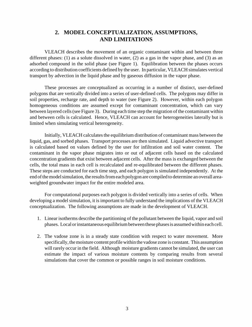
VLEACH describes the movement of an organic contaminant within and between three different phases: (1) as a solute dissolved in water, (2) as a gas in the vapor phase, and (3) as an adsorbed compound in the solid phase (see Figure 1). Equilibration between the phases occurs according to distribution coefficients defined by the user. In particular, VLEACH simulates vertical transport by advection in the liquid phase and by gaseous diffusion in the vapor phase.
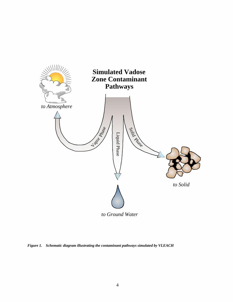
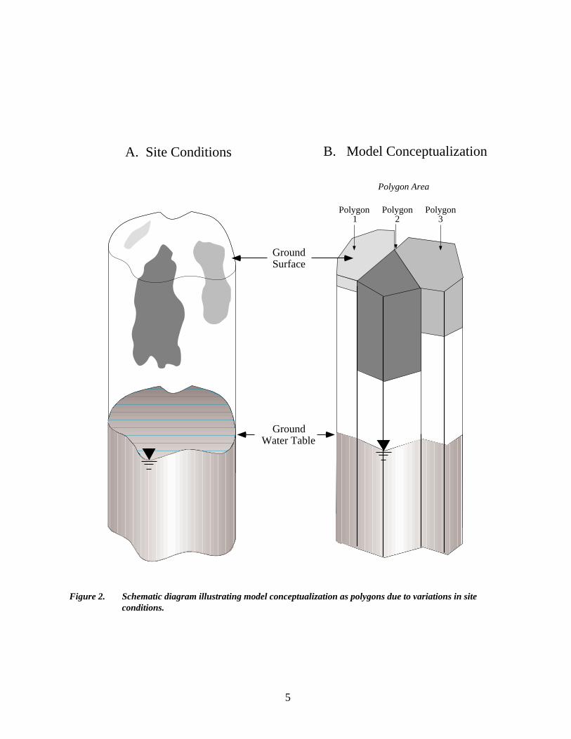
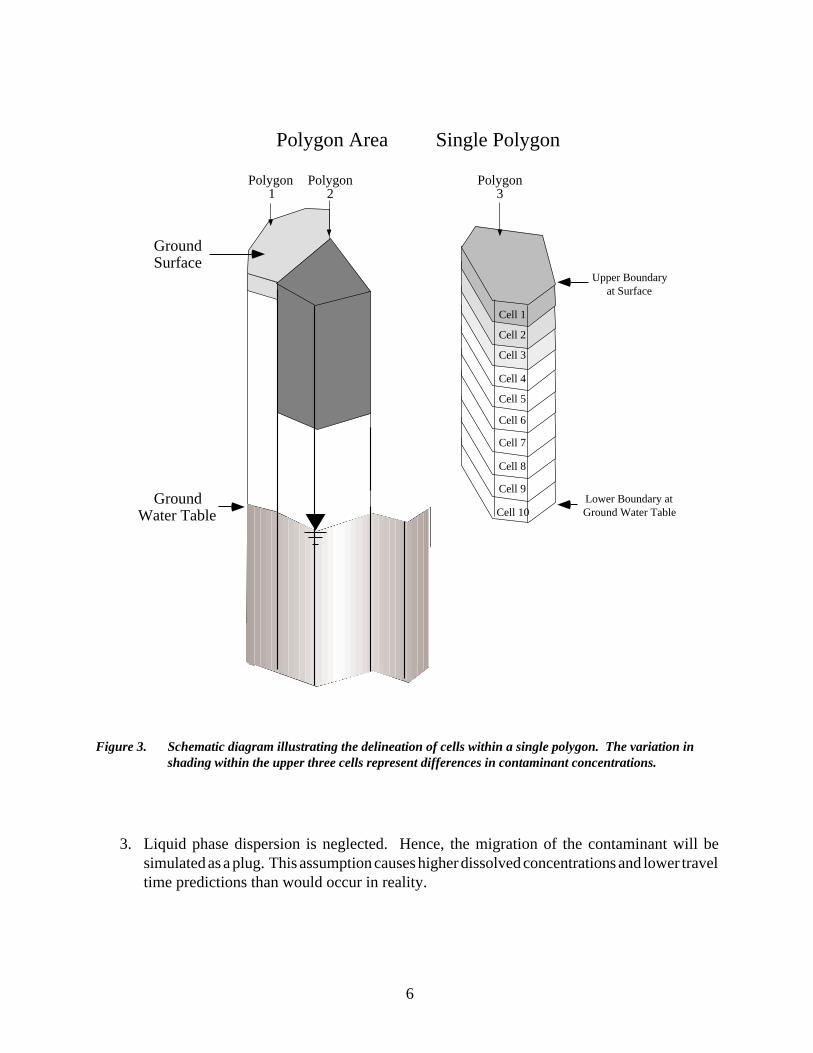
These processes are conceptualized as occurring in a number of distinct, user-defined polygons that are vertically divided into a series of user-defined cells. The polygons may differ in soil properties, recharge rate, and depth to water (see Figure 2). However, within each polygon homogeneous conditions are assumed except for contaminant concentration, which can vary between layered cells (see Figure 3). During each time step the migration of the contaminant within and between cells is calculated. Hence, VLEACH can account for heterogeneities laterally but is limited when simulating vertical heterogeneity.
Initially, VLEACH calculates the equilibrium distribution of contaminant mass between the liquid, gas, and sorbed phases. Transport processes are then simulated. Liquid advective transport is calculated based on values defined by the user for infiltration and soil water content. The contaminant in the vapor phase migrates into or out of adjacent cells based on the calculated concentration gradients that exist between adjacent cells. After the mass is exchanged between the cells, the total mass in each cell is recalculated and re-equilibrated between the different phases. These steps are conducted for each time step, and each polygon is simulated independently. At the end of the model simulation, the results from each polygon are compiled to determine an overall area-weighted groundwater impact for the entire modeled area.
For computational purposes each polygon is divided vertically into a series of cells. When developing a model simulation, it is important to fully understand the implications of the VLEACH conceptualization. The following assumptions are made in the development of VLEACH.
1. Linear isotherms describe the partitioning of the pollutant between the liquid, vapor and soil phases. Local or instantaneous equilibrium between these phases is assumed within each cell.
2. The vadose zone is in a steady state condition with respect to water movement. More specifically, the moisture content profile within the vadose zone is constant. This assumption will rarely occur in the field. Although moisture gradients cannot be simulated, the user can estimate the impact of various moisture contents by comparing results from several simulations that cover the common or possible ranges in soil moisture conditions.
3
to Atmosphere Solid Phase
Phas
e
Vap
or
Liquid Phase
Simulated Vadose Zone Contaminant
Pathways
to Solid
to Ground Water
Figure 1. Schematic diagram illustrating the contaminant pathways simulated by VLEACH
4
A. Site Conditions B. Model Conceptualization
Polygon Area
Polygon Polygon Polygon 1 2 3
Ground Surface
Ground Water Table
Figure 2. Schematic diagram illustrating model conceptualization as polygons due to variations in site conditions.
5
Polygon Area Single Polygon
Polygon Polygon Polygon 1 2 3
Ground Surface
Cell 1
Cell 2
Cell 3
Cell 4
Cell 5
Cell 6
Cell 7
Cell 8
Cell 9
Cell 10
Upper Boundary at Surface
Lower Boundary at Ground Water Table
Ground Water Table
Figure 3. Schematic diagram illustrating the delineation of cells within a single polygon. The variation in shading within the upper three cells represent differences in contaminant concentrations.
3. Liquid phase dispersion is neglected. Hence, the migration of the contaminant will be simulated as a plug. This assumption causes higher dissolved concentrations and lower travel time predictions than would occur in reality.
6
4. The contaminant is not subjected to in situ production or degradation. Since organic contaminants, especially hydrocarbons, generally undergo some degree of degradation in the vadose zone, this assumption results in conservative concentration values.
5. Homogeneous soil conditions are assumed to occur within a particular polygon. This assumption will rarely occur in the field. Although spatial gradients cannot be simulated, the user can estimate the impact of non-uniform soils by comparing results from several simulations covering the range of soil properties present at the site. However, initial contaminant concentrations in the soil phase can vary between cells.
6. Volatilization from the soil boundaries is either completely unimpeded or completely restricted. This assumption may be significant depending upon the depth of investigation and the soil type. In particular, after a depth of 1 meter volatilization to the atmosphere will decrease significantly.
7. The model does not account for non-aqueous phase liquids or any flow conditions derived from variable density.
7

8
bC Z O , = M Z O f a f a , r
1 q
∂C1 ∂ 1q C= -∂t q ∂z
∂C ∂2C g = D g
∂t ∂z2
3. MATHEMATICAL DISCUSSION
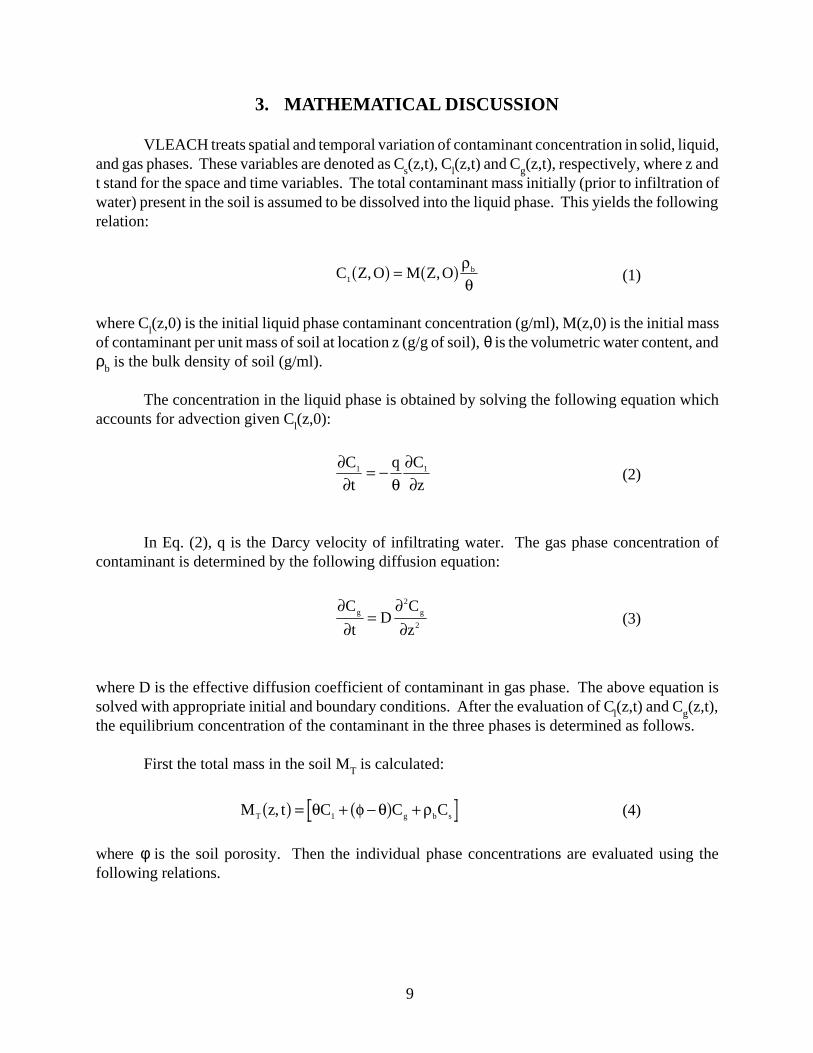
VLEACH treats spatial and temporal variation of contaminant concentration in solid, liquid, and gas phases. These variables are denoted as Cs(z,t), Cl(z,t) and Cg(z,t), respectively, where z and t stand for the space and time variables. The total contaminant mass initially (prior to infiltration of water) present in the soil is assumed to be dissolved into the liquid phase. This yields the following relation:
(1)
where Cl(z,0) is the initial liquid phase contaminant concentration (g/ml), M(z,0) is the initial mass of contaminant per unit mass of soil at location z (g/g of soil), θ is the volumetric water content, and ρb is the bulk density of soil (g/ml).
The concentration in the liquid phase is obtained by solving the following equation which accounts for advection given Cl(z,0):
(2)
In Eq. (2), q is the Darcy velocity of infiltrating water. The gas phase concentration of contaminant is determined by the following diffusion equation:
(3)
where D is the effective diffusion coefficient of contaminant in gas phase. The above equation is solved with appropriate initial and boundary conditions. After the evaluation of Cl(z,t) and Cg(z,t), the equilibrium concentration of the contaminant in the three phases is determined as follows.
First the total mass in the soil MT is calculated:
M z t a f, = qC + a f C + r- Cf q (4)T 1 g b s
where φ is the soil porosity. Then the individual phase concentrations are evaluated using the following relations.
9
K M az t , fH TC z t a f, = g + -a fK + Kq f q rH d b
M z t ,a fC z t a f, = 1 + -a
T
fK + Kq f q rH d b
K M az t , f
C = d T s q f q a fK + K+ - rH d b
f q- 10 3 /a f
=D Dair f2
(5)
(6)
(7)
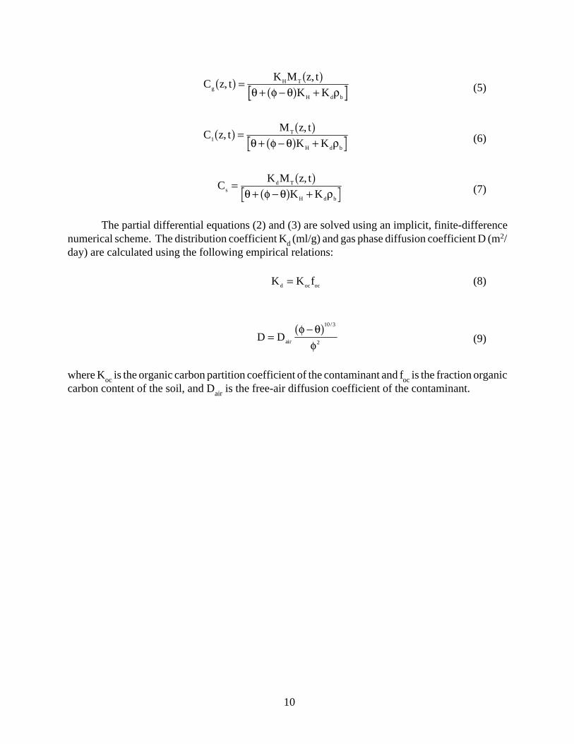
The partial differential equations (2) and (3) are solved using an implicit, finite-difference numerical scheme. The distribution coefficient Kd (ml/g) and gas phase diffusion coefficient D (m2/ day) are calculated using the following empirical relations:
K = K f (8)d oc oc
(9)
where Koc is the organic carbon partition coefficient of the contaminant and foc is the fraction organic carbon content of the soil, and Dair is the free-air diffusion coefficient of the contaminant.
10
4.0 HARDWARE AND SOFTWARE REQUIREMENTS
The minimum hardware and software requirements for VLEACH version 2.0 are:
• IBM-PC or compatible computer with INTEL 8086, 80286, 80386, or 80486 CPU based system
• 256K RAM • Color Graphic Adapter (CGA) board • One floppy disk drive • (MS/PC) DOS 2.0 or higher
Additional recommended hardware annd software include:
• A math coprocessor • A hard disk • A FORTRAN Compiler for modifications of the source code • A commercial graphics software such as Grapher by Golden Software, Inc.
11

12
5.0 GETTING STARTED
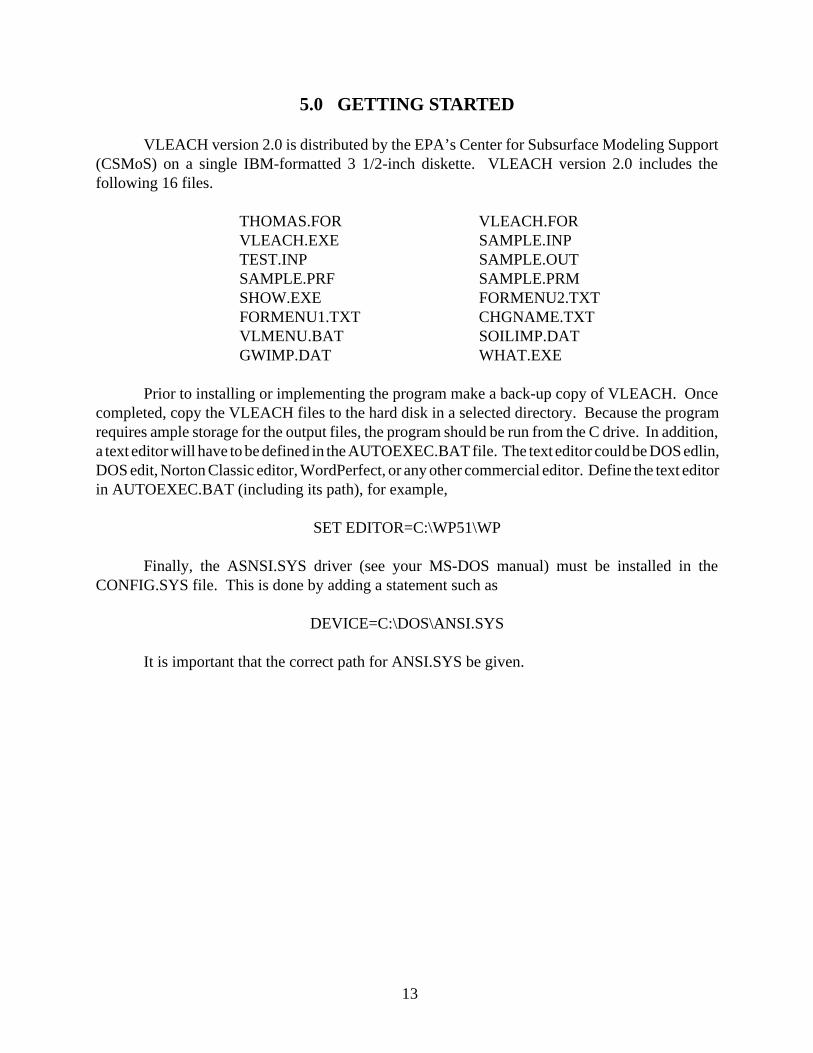
VLEACH version 2.0 is distributed by the EPA’s Center for Subsurface Modeling Support (CSMoS) on a single IBM-formatted 3 1/2-inch diskette. VLEACH version 2.0 includes the following 16 files.
THOMAS.FOR VLEACH.FOR VLEACH.EXE SAMPLE.INP TEST.INP SAMPLE.OUT SAMPLE.PRF SAMPLE.PRM SHOW.EXE FORMENU2.TXT FORMENU1.TXT CHGNAME.TXT VLMENU.BAT SOILIMP.DAT GWIMP.DAT WHAT.EXE
Prior to installing or implementing the program make a back-up copy of VLEACH. Once completed, copy the VLEACH files to the hard disk in a selected directory. Because the program requires ample storage for the output files, the program should be run from the C drive. In addition, a text editor will have to be defined in the AUTOEXEC.BAT file. The text editor could be DOS edlin, DOS edit, Norton Classic editor, WordPerfect, or any other commercial editor. Define the text editor in AUTOEXEC.BAT (including its path), for example,
SET EDITOR=C:\WP51\WP
Finally, the ASNSI.SYS driver (see your MS-DOS manual) must be installed in the CONFIG.SYS file. This is done by adding a statement such as
DEVICE=C:\DOS\ANSI.SYS
It is important that the correct path for ANSI.SYS be given.
13
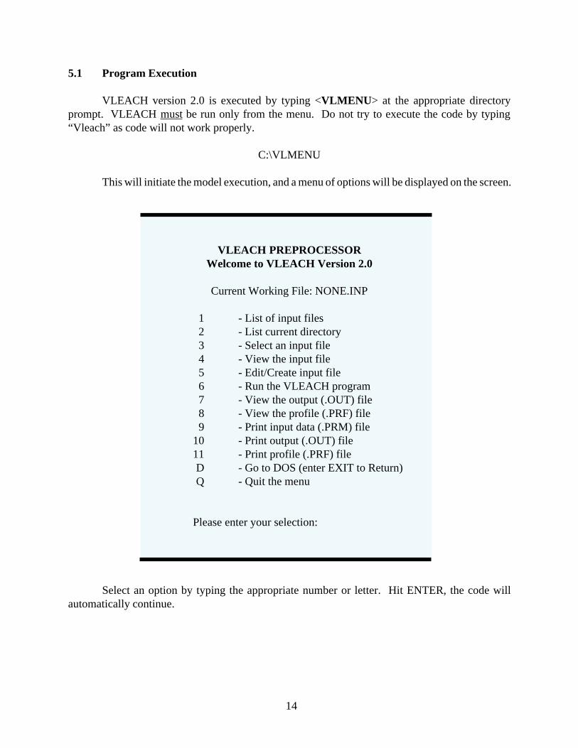
5.1 Program Execution
VLEACH version 2.0 is executed by typing <VLMENU> at the appropriate directory prompt. VLEACH must be run only from the menu. Do not try to execute the code by typing “Vleach” as code will not work properly.
C:\VLMENU
This will initiate the model execution, and a menu of options will be displayed on the screen.
VLEACH PREPROCESSOR Welcome to VLEACH Version 2.0
Current Working File: NONE.INP
1 - List of input files 2 - List current directory 3 - Select an input file 4 - View the input file 5 - Edit/Create input file 6 - Run the VLEACH program 7 - View the output (.OUT) file 8 - View the profile (.PRF) file 9 - Print input data (.PRM) file
10 - Print output (.OUT) file 11 - Print profile (.PRF) file D - Go to DOS (enter EXIT to Return) Q - Quit the menu
Please enter your selection:
Select an option by typing the appropriate number or letter. Hit ENTER, the code will automatically continue.
14
6.0 INPUT PARAMETERS
The following describes the input parameters for VLEACH. It is important that this information be fully understood for proper application of the code. The input parameters for VLEACH consist of two groups, simulation data and polygon-specific data. The simulation data are defined once per model run while the polygon-specific data are defined for per each polygon. In the parameter descriptions below, the FORTRAN format, which is used in data entry, is presented in order of designation per card for the input data.
6.1 Simulation Data
a. Title. A title of up to 80 characters can be defined that describes the simulation. The title will be printed with each output file. [Card 1: TITLE (A80)]
b. Number of Polygons. The number of polygons conceptualized for the site. Each polygon will have a unique set of parameter data. [Card 2: NPOLY (I3)]
c. Timestep. The model timestep given in years. [Card 3: DELT (G10.0)]
d. Simulation Time. The total time length of the simulation given in years. [Card 3: STIME (G10.0)]
e. Output Time Interval. The time interval at which the ground-water impact and mass balance results are printed to the .OUT file. The output time interval is in years. [Card 3: PTIME (G10.0)]
f. Profile Time Interval. The time interval at which the vertical concentration profile results are printed to the .PRF file. The profile time interval is in years. [Card 3: PRTIME (G10.0)]
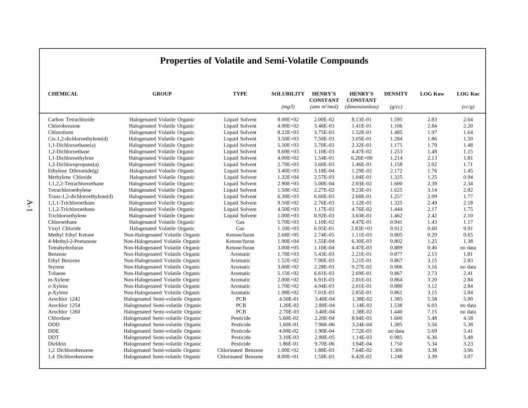
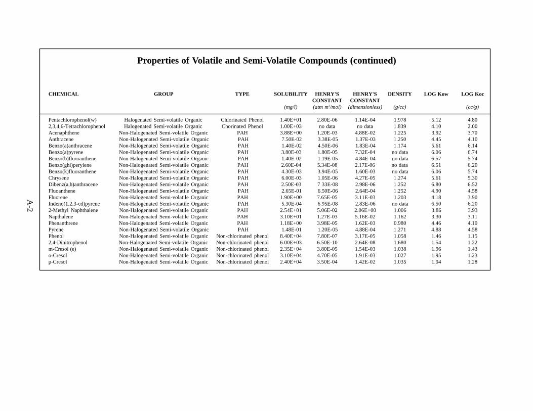
g. Organic Carbon Distribution Coefficient (Koc). The organic carbon distribution coefficient describes the partitioning of the contaminant with organic carbon. The coefficient is in units of ml/g. Appendix A lists the values of Koc for numerous contaminants. If data regarding the pollutant being modeled is not presented refer to the standard reference manuals that are documented in Appendix C or consult the manufacturer of the compound. [Card 4: KOC (G10.0)]
h. Henry’s Constant (KH). Henry’s constant is an empirical constant that describes the liquid-gas partitioning of the contaminant. Henry’s constant is a function of the solubility and partial vapor pressure of the contaminant at a given temperature. VLEACH utilizes the dimensionless form of Henry’s constant given as
M/L3AIR
M/L3 WATER
15
The dimensionless form of KH can be determined from the more common form having the units of atmospheres-cubic meters per mole (atm-m3/mol) using the following equation
KH = KH’/ 0.0246 at 27oC
where KH is dimensionless and KH’ is in units of atm-m3/mol. Data regarding Henry’s Law Constant for over 60 common volatile and semi-volatile organic compounds are provided in Appendix A. [Card 4: KH (G10.0)]
i. Water Solubility. Values defining the water solubility of the contaminant must have units of milligrams per liter (mg/L). Appendix A provides water water solubility information for over 60 compounds. [Card 4: CMAX (G10.0)]
j. Free Air Diffusion Coefficient. The free air diffusion coefficient describes transfer of the contaminant due to Brownian motion in the air phase. The coefficient is in meter2 per day (m2/day). For information regarding the free air diffusion coefficient refer to Bird et al. (1960)(pp. 503-514), or any similar reference text. [Card 4: DAIR (G10.0)]
6.2 Polygon Data (this set is repeated NPOLY times)
For each polygon input values for the following parameters are needed.
k. Title. A title of up to 80 characters can be defined that describes the simulation. The title will be printed with each output file. [Card 1: TITLE (A80)]
l. Area. This parameter defines the area of the polygon in square feet. [Card 2: AREA (G10.0)]
m. Vertical Cell Dimension. This parameter defines the vertical height of the cells within the polygon. The cell dimension is in feet. [Card 2: DELZ (G10.0)]
n. Recharge Rate. The groundwater recharge rate describes the velocity of water movement through the vadose zone. The rate is given in feet per year. In the vadose zone the hydraulic conductivity of the soil is an increasing function of the water content of the soil. Hence, the ground water recharge rate should be equal to or lower than the hydraulic conductivity of the soil at the modeled water content. It should be noted that this parameter is extremely difficult to estimate as in reality it will vary with respect to time. It is strongly suggested that a range of possible recharge values be utilized to evaluate the potential variability of the results due to uncertainty associated with this parameter. [Card 2: Q (G10.0)]
16
o. Dry Bulk Density. This parameter describes the mass of dry soil relative to the bulk volume of soil. It is described in units of grams per cubic centimeters (g/cm3). Ranges for bulk density with respect to different soil types are given in Appendix B. [Card 2: RHOB (G10.0)]
p. Effective Porosity. The effective porosity describes the volume of void space within the soil that is potentially fillable with water. The effective porosity equals total porosity minus irreducible water content, that percentage of total volume that water is retained due to capillary forces (see Appendix B). Effective porosity is a dimensionless parameter. [Card 2: POR (G10.0)]
q. Volumetric Water Content. The water content of the soil in percent total volume. This parameter is assumed constant in time and space, however, this rarely occurs in nature. The volumetric water content can neither exceed the porosity of the soil nor be lower than the irreducible soil water content. [Card 2: THETA (G10.0)]
r. Soil Organic Carbon Content. The fraction organic content of the soil is the relative amount of organic carbon present in the soil. This parameter defines the amount of potential adsorbtive sites for the contaminant in the solid phase. The fraction organic content can be determined from laboratory analyses or is documented in some soil descriptions of the Soil Conservation Service. Generic values for organic content for soils of different texture are listed in Appendix B. [Card 2: FOC (G10.0)]
s. Concentration of Recharge Water. This parameter defines the contaminant concentration in milligrams per liter (mg/L). If the recharge water is derived from precipitation the contaminant concentration will typically be set at zero. [Card 3: CINF (G10.0)]
t. Upper Boundary Condition for Vapor. This parameter defines the contaminant concentration in mg/L in the atmosphere above the soil surface. If the upper boundary of the polygon is considered impermeable to gas diffusion enter a negative value. [Card 3: CATM (G10.0)]
u. Lower Boundary Vapor Condition for Vapor. This parameter defines the contaminant concentration in mg/L in the ground water at the base of the vadose zone. If the lower boundary of the polygon is considered impermeable to gas diffusion enter a negative value. [Card 3: CGW (G10.0)]
v. Cell Number. The cell number defines the number of cells within the polygon. The number of cells is equal to the polygon height divided by the Cell Vertical Dimension. [Card 4: NCELL (I5)]
w. Plot Variable. Variable to denote the plotting option. “Y” or “y” indicates that a plot file containing the soil contaminant profile will be created. [Card 4: PLT (A1)]
17
aaaaaaaaaaaaaaaaaaaaaaaaaaaaaaaaaaaaaaaaaaaaaaaaaaaaaaaaaaaaaaaaaaaaaaaaaaaaaaaa
bbb
ccccccccccddddddddddeeeeeeeeeeffffffffff
gggggggggghhhhhhhhhhiiiiiiiiiijjjjjjjjjj
kkkkkkkkkkkkkkkkkkkkkkkkkkkkkkkkkkkkkkkkkkkkkkkkkkkkkkkkkkkkkkkkkkkkkkkkkkkkkkkk
llllllllllmmmmmmmmmmnnnnnnnnnnooooooooooppppppppppqqqqqqqqqqrrrrrrrrrr
ssssssssssttttttttttuuuuuuuuuu
vvvvvwxxxxxxxxxx
*****#####$$$$$$$$$$
x. Plot Time. Plot time defines the time in years for which the soil contaminant profile data will be created for the plot file. [Card 4: PLTIME (G10.0)]
y. Initial Contaminant Concentration. This value defines the initial contaminant concentration in the soil within a single or set of cells. The concentration is given in units of micrograms per kilogram (ug/kg). The input is given by recording the number of the upper and the lower cells (J1 and J2, respectively) and the defined concentration (XCON) in those cells. The initial contaminant concentration must be defined for all cells within the polygon. [Card 5: J1,J2, XCON (2I5,G10.0) Card 5 is repeated as necessary until each cell has been described and the bottom cell (J2) equals the Cell Number (NCELL)].
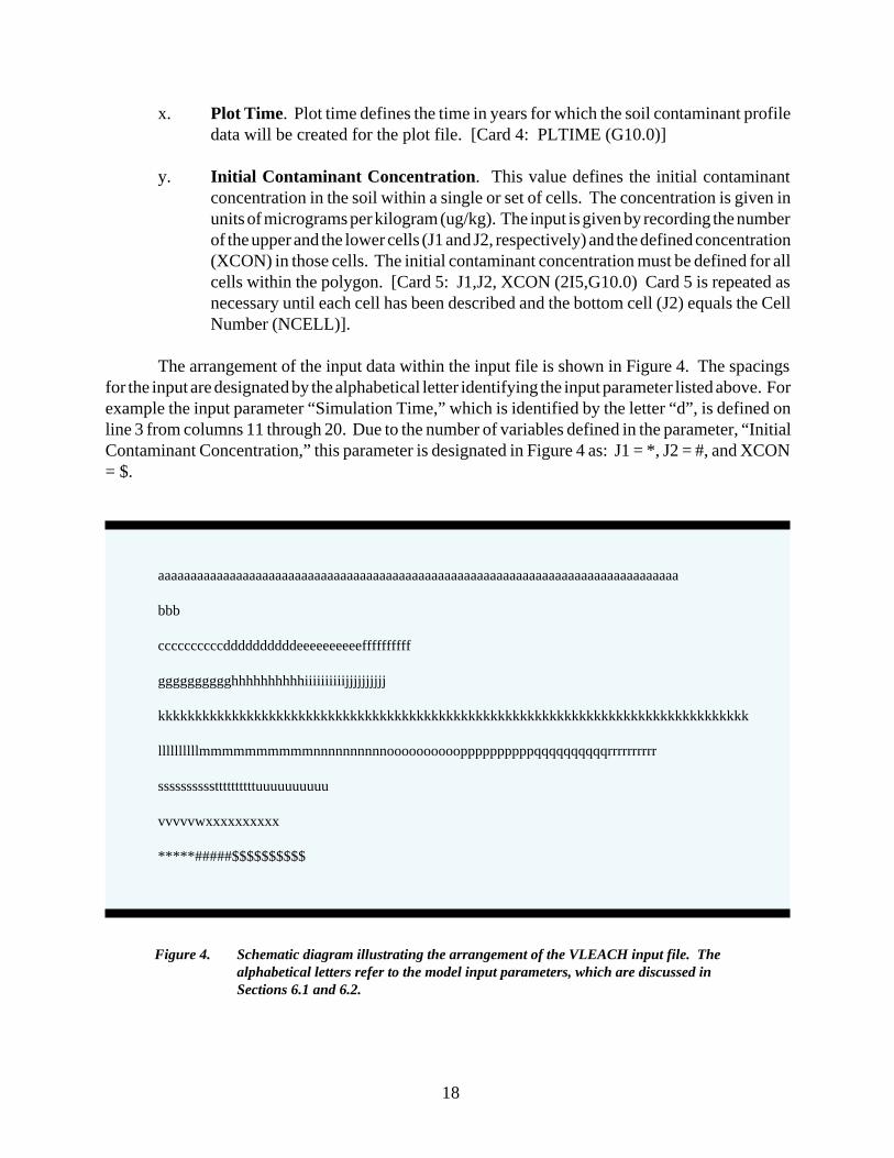
The arrangement of the input data within the input file is shown in Figure 4. The spacings for the input are designated by the alphabetical letter identifying the input parameter listed above. For example the input parameter “Simulation Time,” which is identified by the letter “d”, is defined on line 3 from columns 11 through 20. Due to the number of variables defined in the parameter, “Initial Contaminant Concentration,” this parameter is designated in Figure 4 as: J1 = *, J2 = #, and XCON = $.
Figure 4. Schematic diagram illustrating the arrangement of the VLEACH input file. The alphabetical letters refer to the model input parameters, which are discussed in Sections 6.1 and 6.2.
18
Sample Problem - TCE contamination scenario 1 polygons
Timestep = 10.00 years. Simulation length = 500.00 years Printout every 100.00 years. Vertical profile stored every 250.00 years. Koc = 100.00 ml/g, .35314E-02cu.ft./g Kh = .40000 (dimensionless). Aqueous solubility = 1100.0 mg/l, 31.149 g/cu.ft Free air diffusion coefficient = .70000 sq. m/day, 2750.3 sq.ft./yr
Polygon 1 Polygon I Polygon area = 1000.0 sq. ft 50 cells, each cell 1.00 ft. thick. Soil Properties: Bulk density = 1.6000 g/ml 45307 g/cu.ft. Porosity = .4000 Volumetric water content = .3000 Organic carbon content = .3000 Recharge Rate = 1.00000000 ft/yr Conc. in recharge water = .00000 mg/l, .00000 g/cu.ft Atmospheric concentration = .00000 mg/l, .00000 g/cu.ft Water table has a fixed concentration of .00000 mg/l, .00000 g/cu.ft with respect to gas diffusion.
7.0 OUTPUT
7.1 Output Options
An option can be defined by the user to convert the output from VLEACH into files that can be plotted using GRAPHER (Golden Software, 1987) or other compatible commercial graphics packages. Two graphs can be constructed: a groundwater impact curve and a soil-depth contaminant concentration profile. These can be selected by defining a “Y” or “y” for the input parameter, Plot Variable, (see Section 6.2.w). This creates two ASCII data files in X-Y format, GWIMP.DAT and SOILIMP.DAT. If plots are desired then input the time in years at which the soil concentration profile will be defined for the Plot Time Variable (see Section 6.2.x).
7.2 Output Results
VLEACH output provides information regarding the input parameters, the physical nature of the vapor, liquid, and solid contaminant mass balances in the soil, ground-water impacts from the contaminant, and the concentration profile of the contaminant within the soil profile. The output consists of three different files having the extensions .PRM, .OUT, and .PRF. The code allows the user to view the output as well as to print the output. These options can be selected from the main menu screen.
7.2.1 _____.PRM File
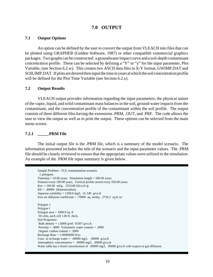
The initial output file is the .PRM file, which is a summary of the model scenario. The information presented includes the title of the scenario and the input parameter values. The .PRM file should be closely reviewed to ensure that the appropriate values were utilized in the simulation. An example of the .PRM file input summary is given below.
19
7.2.2 _____.OUT File
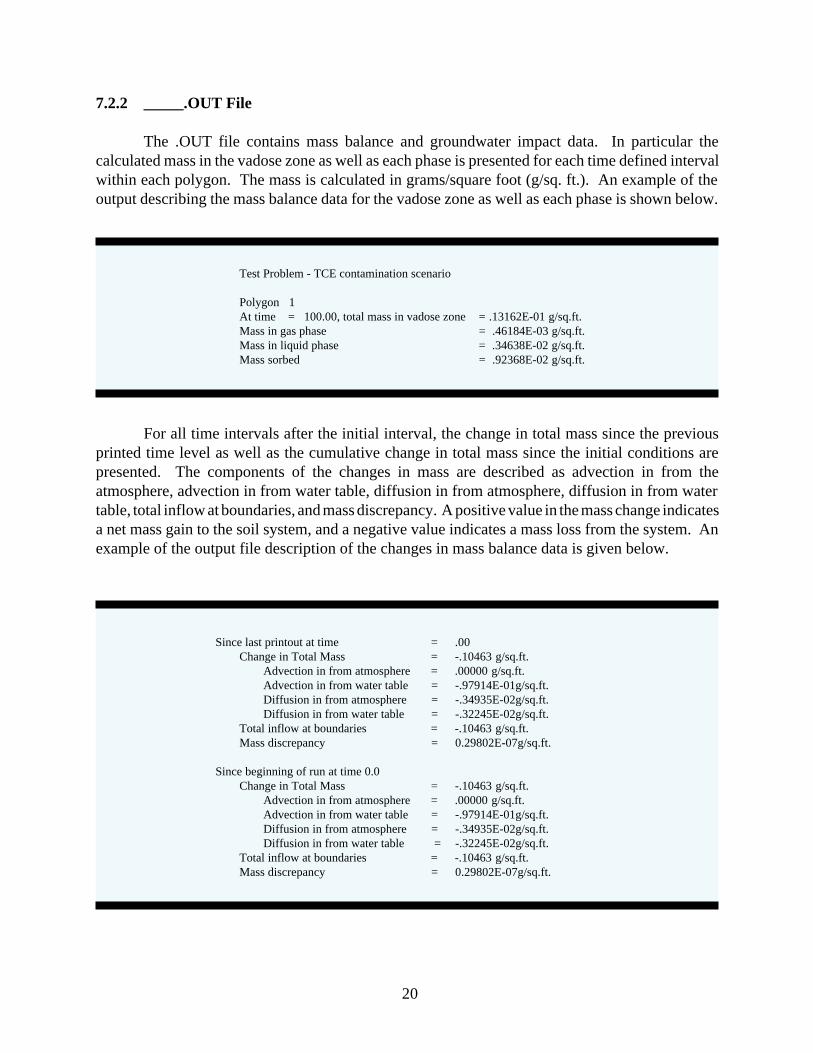
The .OUT file contains mass balance and groundwater impact data. In particular the calculated mass in the vadose zone as well as each phase is presented for each time defined interval within each polygon. The mass is calculated in grams/square foot (g/sq. ft.). An example of the output describing the mass balance data for the vadose zone as well as each phase is shown below.
Test Problem - TCE contamination scenario
Polygon 1 At time = 100.00, total mass in vadose zone Mass in gas phase Mass in liquid phase Mass sorbed
= .13162E-01 g/sq.ft. = .46184E-03 g/sq.ft. = .34638E-02 g/sq.ft. = .92368E-02 g/sq.ft.
For all time intervals after the initial interval, the change in total mass since the previous printed time level as well as the cumulative change in total mass since the initial conditions are presented. The components of the changes in mass are described as advection in from the atmosphere, advection in from water table, diffusion in from atmosphere, diffusion in from water table, total inflow at boundaries, and mass discrepancy. A positive value in the mass change indicates a net mass gain to the soil system, and a negative value indicates a mass loss from the system. An example of the output file description of the changes in mass balance data is given below.
Since last printout at time = .00 Change in Total Mass = -.10463 g/sq.ft.
Advection in from atmosphere = .00000 g/sq.ft. Advection in from water table = -.97914E-01g/sq.ft. Diffusion in from atmosphere = -.34935E-02g/sq.ft. Diffusion in from water table = -.32245E-02g/sq.ft.
Total inflow at boundaries = -.10463 g/sq.ft. Mass discrepancy = 0.29802E-07g/sq.ft.
Since beginning of run at time 0.0 Change in Total Mass = -.10463 g/sq.ft.
Advection in from atmosphere = .00000 g/sq.ft. Advection in from water table = -.97914E-01g/sq.ft. Diffusion in from atmosphere = -.34935E-02g/sq.ft. Diffusion in from water table = -.32245E-02g/sq.ft.
Total inflow at boundaries = -.10463 g/sq.ft. Mass discrepancy = 0.29802E-07g/sq.ft.
20
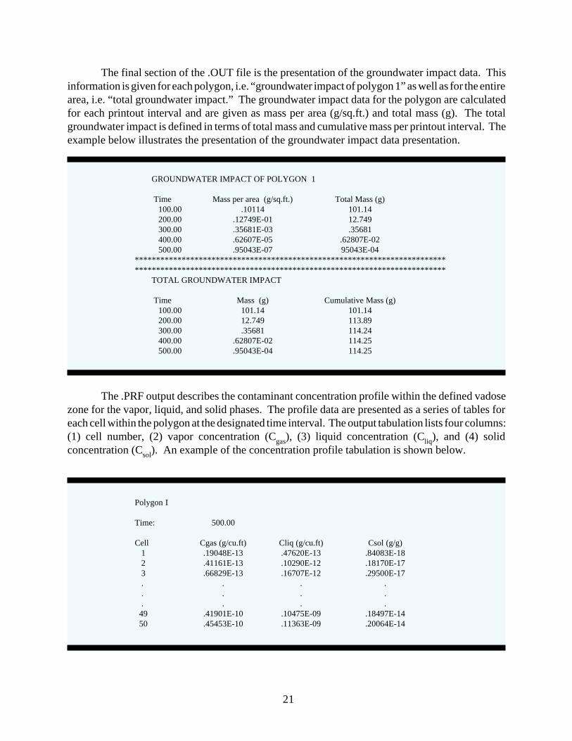
The final section of the .OUT file is the presentation of the groundwater impact data. This information is given for each polygon, i.e. “groundwater impact of polygon 1” as well as for the entire area, i.e. “total groundwater impact.” The groundwater impact data for the polygon are calculated for each printout interval and are given as mass per area (g/sq.ft.) and total mass (g). The total groundwater impact is defined in terms of total mass and cumulative mass per printout interval. The example below illustrates the presentation of the groundwater impact data presentation.
GROUNDWATER IMPACT OF POLYGON 1
Time Mass per area (g/sq.ft.) Total Mass (g) 100.00 .10114 101.14 200.00 .12749E-01 12.749 300.00 .35681E-03 .35681 400.00 .62607E-05 .62807E-02 500.00 .95043E-07 95043E-04
************************************************************************* *************************************************************************
TOTAL GROUNDWATER IMPACT
Time Mass (g) Cumulative Mass (g) 100.00 101.14 101.14 200.00 12.749 113.89 300.00 .35681 114.24 400.00 .62807E-02 114.25 500.00 .95043E-04 114.25
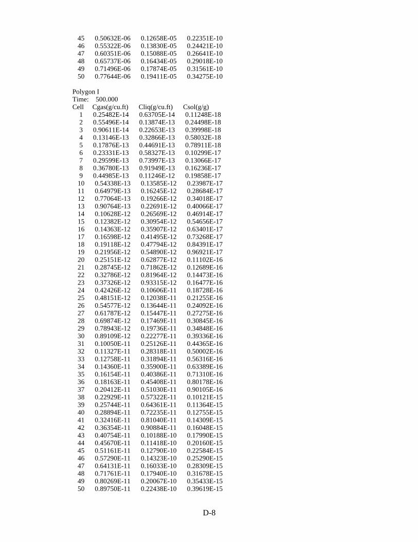
The .PRF output describes the contaminant concentration profile within the defined vadose zone for the vapor, liquid, and solid phases. The profile data are presented as a series of tables for each cell within the polygon at the designated time interval. The output tabulation lists four columns: (1) cell number, (2) vapor concentration (Cgas), (3) liquid concentration (Cliq), and (4) solid concentration (Csol). An example of the concentration profile tabulation is shown below.
Polygon I
Time: 500.00
Cell Cgas (g/cu.ft) Cliq (g/cu.ft) Csol (g/g) 1 .19048E-13 .47620E-13 .84083E-18 2 .41161E-13 .10290E-12 .18170E-17 3 .66829E-13 .16707E-12 .29500E-17 . . . . . . . . . . . .
49 .41901E-10 .10475E-09 .18497E-14 50 .45453E-10 .11363E-09 .20064E-14
21
7.3 Graphical Output Displays
Using commercial graphics packages two graphs can be plotted using the output from the model simulation. VLEACH automatically writes output data to two files named GWIMP.DAT and SOILIMP.DAT for plotting purposes. The file GWIMP.DAT contains the mass rate of contaminant loading to the groundwater versus time array. When plotted the mass loading is defined on the Y-axis while time is defined on the X-axis. The file SOILIMP.DAT contains the values for contaminant concentration sorbed to the soil versus depth array for the specified time period. When plotted the contaminant concentration is defined on the X-axis and depth is given on the Y-axis. Examples of the plots are shown in the Sample Problem, Section 9.0.
22
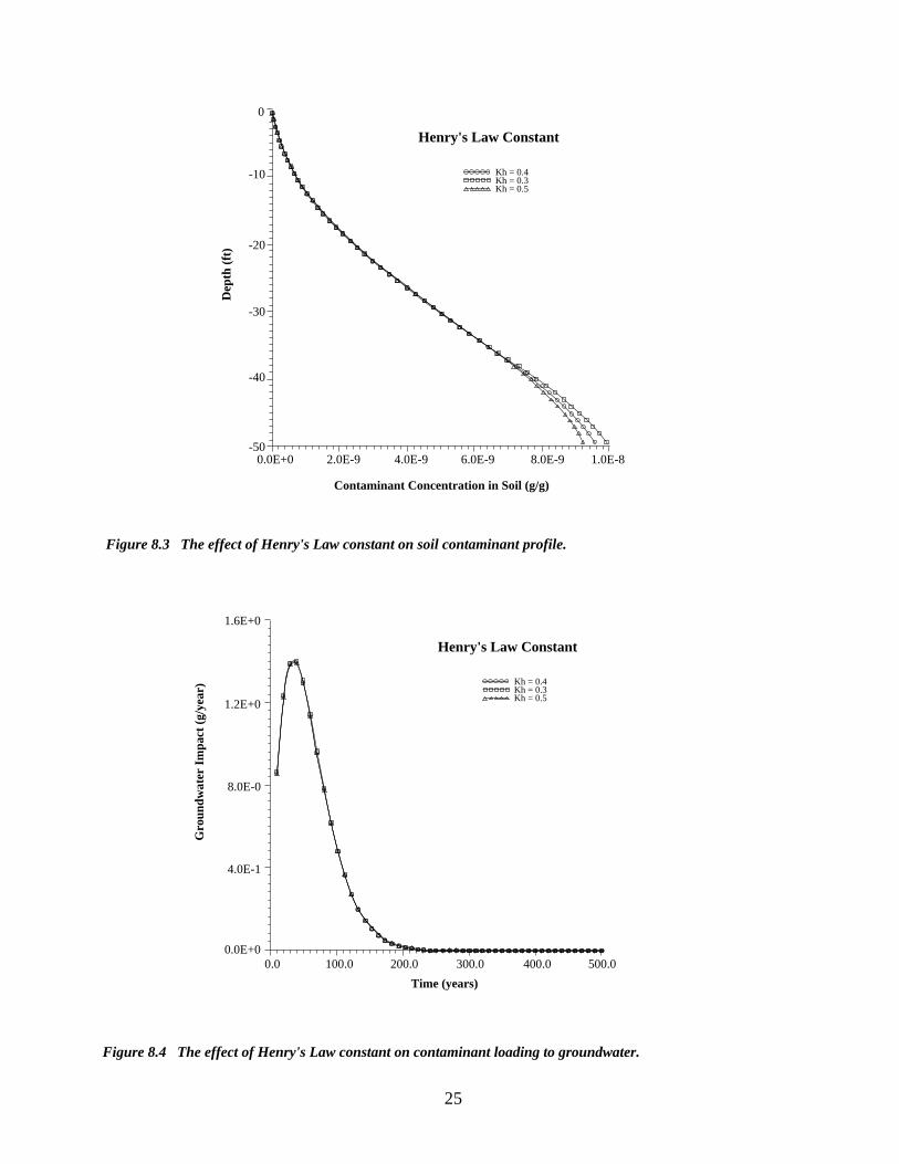
8.0 SENSITIVITY ANALYSIS
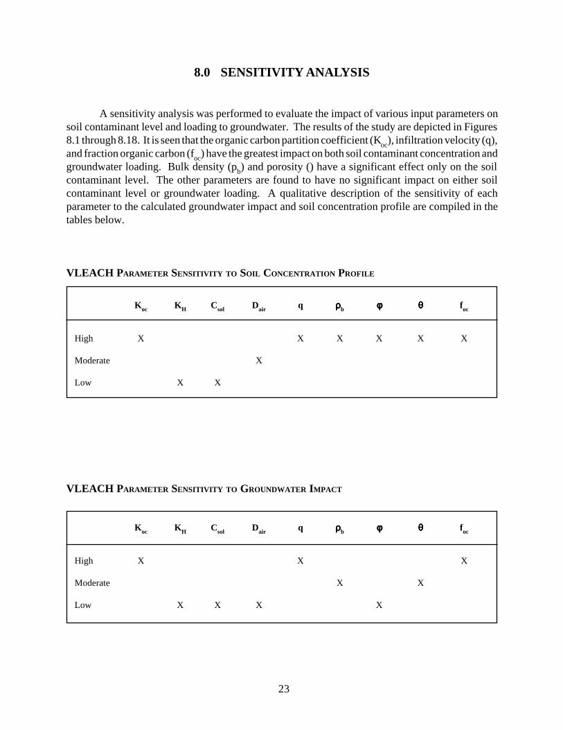
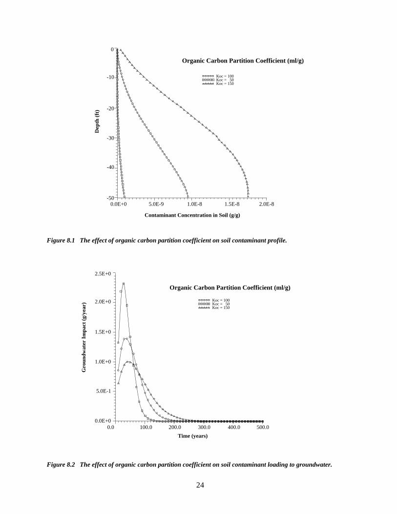
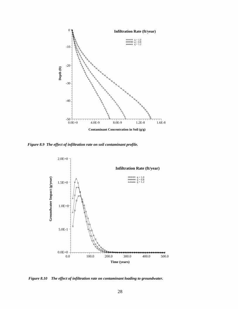
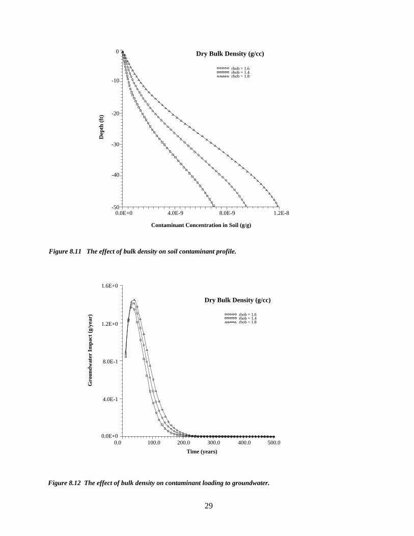
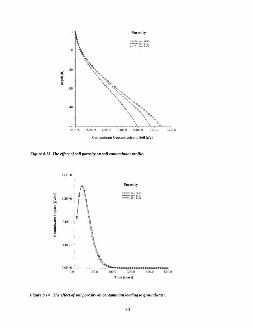
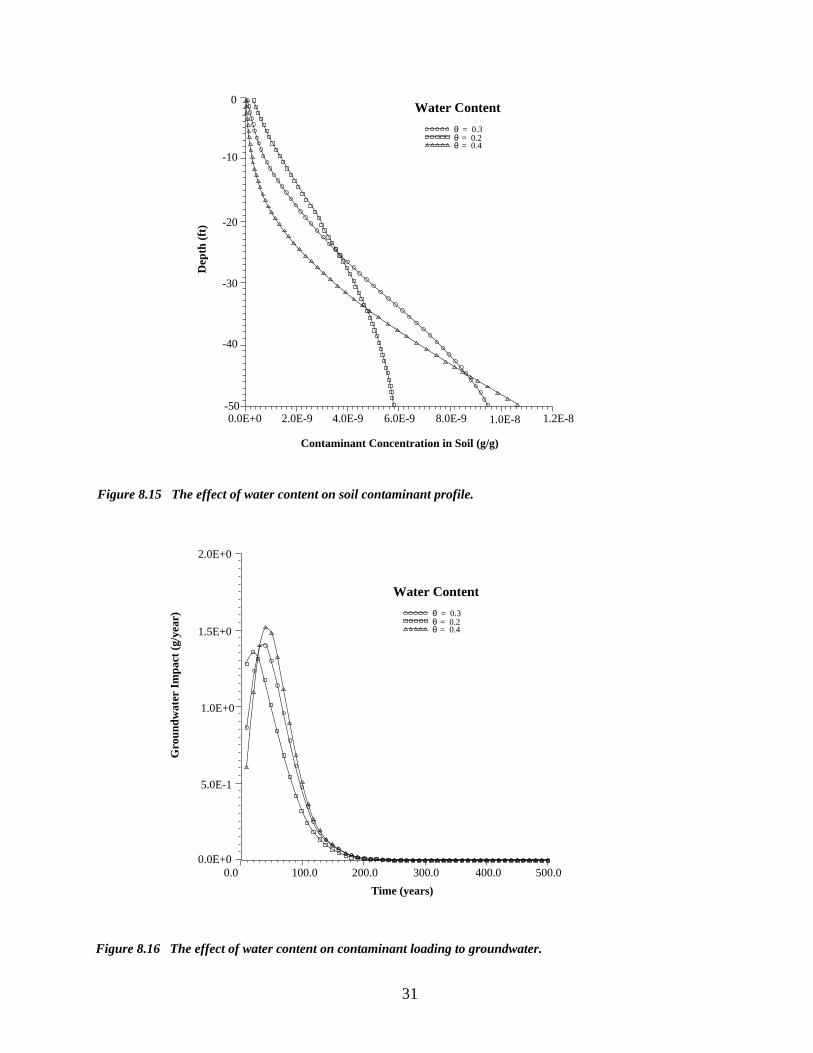
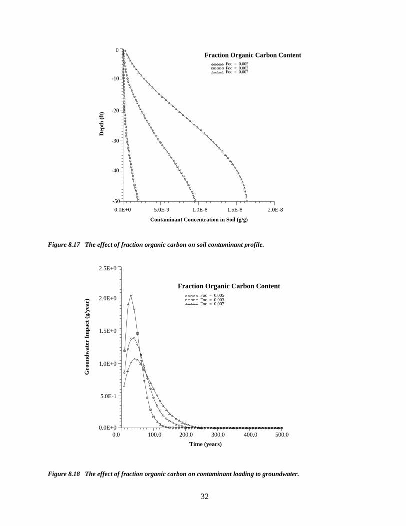
A sensitivity analysis was performed to evaluate the impact of various input parameters on soil contaminant level and loading to groundwater. The results of the study are depicted in Figures 8.1 through 8.18. It is seen that the organic carbon partition coefficient (Koc), infiltration velocity (q), and fraction organic carbon (foc) have the greatest impact on both soil contaminant concentration and groundwater loading. Bulk density (pb) and porosity () have a significant effect only on the soil contaminant level. The other parameters are found to have no significant impact on either soil contaminant level or groundwater loading. A qualitative description of the sensitivity of each parameter to the calculated groundwater impact and soil concentration profile are compiled in the tables below.
VLEACH PARAMETER SENSITIVITY TO SOIL CONCENTRATION PROFILE
K oc KH Csol Dair q ρρρρρb φφφφφ θθθθθ f oc
High X X X X X X
Moderate X
Low X X
VLEACH PARAMETER SENSITIVITY TO GROUNDWATER IMPACT
K oc KH Csol Dair q ρρρρρb φφφφφ θθθθθ f oc
High X X X
Moderate X X
Low X X X X
23
0
-10
-20
-30
-40
-50 0.0E+0 5.0E-9 1.0E-8 1.5E-8 2.0E-8
Contaminant Concentration in Soil (g/g)
Dep
th (
ft)
Organic Carbon Partition Coefficient (ml/g)
Koc = 100 Koc = 50 Koc = 150
Figure 8.1 The effect of organic carbon partition coefficient on soil contaminant profile.
2.5E+0
Gro
undw
ater
Im
pact
(g/
year
)
0.0E+0
Organic Carbon Partition Coefficient (ml/g)
Koc = 100 Koc = 50 Koc = 150
500.0
5.0E-1
1.0E+0
1.5E+0
2.0E+0
0.0 100.0 200.0 300.0 400.0
Time (years)
Figure 8.2 The effect of organic carbon partition coefficient on soil contaminant loading to groundwater.
24
0
-10
-20
-30
-40
-50 0.0E+0 2.0E-9 4.0E-9
Contaminant Concentration in Soil (g/g)
Dep
th (
ft)
Henry's Law Constant
Kh = 0.4 Kh = 0.3 Kh = 0.5
6.0E-9 8.0E-9 1.0E-8
1.6E+0
Figure 8.3 The effect of Henry's Law constant on soil contaminant profile.
Gro
undw
ater
Im
pact
(g/
year
)
1.2E+0
8.0E-0
4.0E-1
0.0E+0 500.0
Henry's Law Constant
Kh = 0.4 Kh = 0.3 Kh = 0.5
0.0 100.0 200.0 300.0 400.0
Time (years)
Figure 8.4 The effect of Henry's Law constant on contaminant loading to groundwater.
25
0
-10
-20
-30
-40
-50 0.0E+0 2.0E-9 4.0E-9
Contaminant Concentration in Soil (g/g)
Dep
th (
ft)
Water Solubility (mg/l)
Csol = 1100 Csol = 900 Csol = 1300
6.0E-9 8.0E-9 1.0E-8
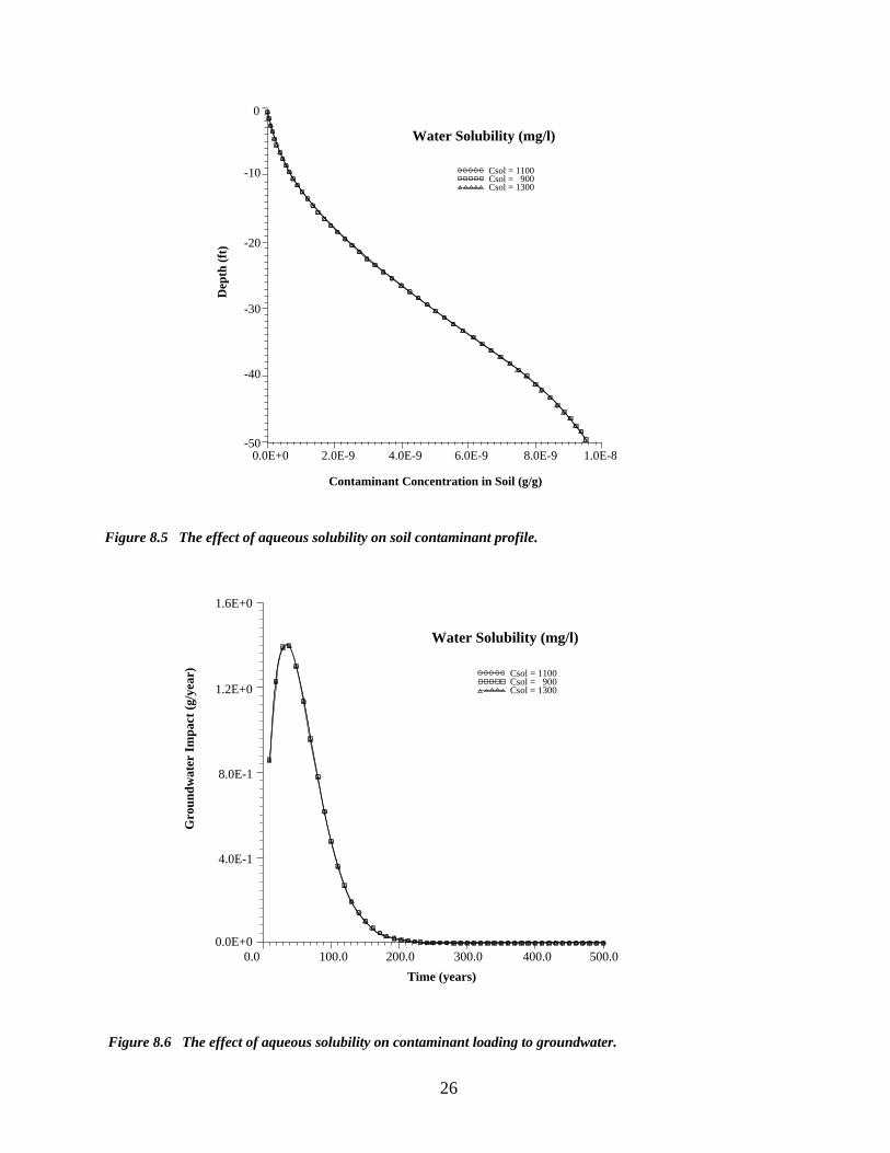
Figure 8.5 The effect of aqueous solubility on soil contaminant profile.
1.6E+0
Gro
undw
ater
Im
pact
(g/
year
)
Water Solubility (mg/l)
Csol = 1100 Csol = 900 Csol = 1300
0.0E+0 500.0
4.0E-1
8.0E-1
1.2E+0
0.0 100.0 200.0 300.0 400.0
Time (years)
Figure 8.6 The effect of aqueous solubility on contaminant loading to groundwater.
26
0
-10
-20
-30
-40
-50 0.0E+0 2.0E-9 4.0E-9
Contaminant Concentration in Soil (g/g)
Dep
th (
ft)
Free-Air Diffusion Coefficient (sq. m/d)
Da tr = 0.7 Da tr = 0.4 Da tr = 1.0
6.0E-9 8.0E-9 1.0E-8
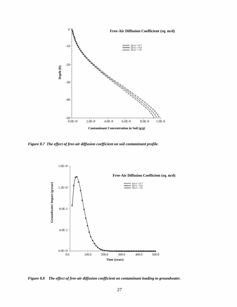
Figure 8.7 The effect of free-air diffusion coefficient on soil contaminant profile.
1.6E+0
Gro
undw
ater
Im
pact
(g/
year
)
Free-Air Diffusion Coefficient (sq. m/d)
Da tr = 0.7 Da tr = 0.4 Da tr = 1.0
0.0E+0 500.0
4.0E-1
8.0E-1
1.2E+0
0.0 100.0 200.0 300.0 400.0
Time (years)
Figure 8.8 The effect of free-air diffusion coefficient on contaminant loading to groundwater.
27
2.0E+0
0
-10
-20
-30
-40
-50 0.0E+0 4.0E-9 8.0E-9
Contaminant Concentration in Soil (g/g)
Dep
th (
ft)
1.2E-8 1.6E-8
Infiltration Rate (ft/year)
q = 1.0q = 0.8 q = 1.2
Figure 8.9 The effect of infiltration rate on soil contaminant profile.
Gro
undw
ater
Im
pact
(g/
year
)
Infiltration Rate (ft/year)
q = 1.0q = 0.8q = 1.2
0.0E+0 500.0
5.0E-1
1.0E+0
1.5E+0
0.0 100.0 200.0 300.0 400.0
Time (years)
Figure 8.10 The effect of infiltration rate on contaminant loading to groundwater.
28
0
-10
-20
-30
-40
-50 0.0E+0 4.0E-9 8.0E-9
Contaminant Concentration in Soil (g/g)
Dep
th (
ft)
1.2E-8
Dry Bulk Density (g/cc)
rhob = 1.6 rhob = 1.4 rhob = 1.8
1.6E+0
Figure 8.11 The effect of bulk density on soil contaminant profile.
Gro
undw
ater
Im
pact
(g/
year
)
Dry Bulk Density (g/cc)
rhob = 1.6 rhob = 1.4 rhob = 1.8
0.0E+0 500.0
4.0E-1
8.0E-1
1.2E+0
0.0 100.0 200.0 300.0 400.0
Time (years)
Figure 8.12 The effect of bulk density on contaminant loading to groundwater.
29
0
-10
-20
-30
-40
-50 0.0E+0 4.0E-9 8.0E-9
Dep
th (
ft)
1.2E-8
Porosity
φ = 0.40 φ = 0.35 φ = 0.45
2.0E-9 6.0E-9 1.0E-8
Contaminant Concentration in Soil (g/g)
Figure 8.13 The effect of soil porosity on soil contaminant profile.
1.6E+0
Gro
undw
ater
Im
pact
(g/
year
)
0.0E+0 0.0 100.0 200.0 300.0 400.0
Time (years)
500.0
4.0E-1
8.0E-1
1.2E+0
Porosity
φ = 0.40 φ = 0.35 φ = 0.45
Figure 8.14 The effect of soil porosity on contaminant loading to groundwater.
30
0
-10
-20
-30
-40
-50 0.0E+0 4.0E-9 8.0E-9
Dep
th (
ft)
1.2E-8
Water Content
θ = 0.3 θ = 0.2 θ = 0.4
2.0E-9 6.0E-9 1.0E-8
Contaminant Concentration in Soil (g/g)
Figure 8.15 The effect of water content on soil contaminant profile.
2.0E+0
Gro
undw
ater
Im
pact
(g/
year
)
Water Content
θ = 0.3 θ = 0.2 θ = 0.4
0.0E+0 0.0 100.0 200.0 300.0 400.0
Time (years)
500.0
5.0E-1
1.0E+0
1.5E+0
Figure 8.16 The effect of water content on contaminant loading to groundwater.
31
0
-10
-20
-30
-40
-50
0.0E+0 1.0E-8 2.0E-8
Dep
th (
ft)
Fraction Organic Carbon Content Foc = 0.005 Foc = 0.003 Foc = 0.007
5.0E-9 1.5E-8
Contaminant Concentration in Soil (g/g)
Figure 8.17 The effect of fraction organic carbon on soil contaminant profile.
2.5E+0
Gro
undw
ater
Im
pact
(g/
year
)
0.0E+0 0.0 100.0 200.0 300.0 400.0
Time (years)
500.0
5.0E-1
1.0E+0
1.5E+0
Fraction Organic Carbon Content Foc = 0.005 Foc = 0.003 Foc = 0.007
2.0E+0
Figure 8.18 The effect of fraction organic carbon on contaminant loading to groundwater.
32
9.0 SAMPLE PROBLEM
The following application of VLEACH is based on a hypothetical scenario. The scenario deals with evaluating TCE contamination of an aquifer that is located 50 feet below the soil surface. The soil is initially (prior to infiltration) contaminated with TCE, and the soil concentration along the depth is given as below:
DEPTH (ft) TCE CONCENTRATION (µg/kg of soil)
1 - 20 100 20 - 30 50 30 - 40 10 40 - 50 0
The area of the contamination is 1000 square feet. The recharge rate to groundwater is 1 foot per year. The other soil, chemical, and computational parameters required for the execution of the model are presented below. These parameters are the same as that appearing in the input file, SAMPLE.INP.
Model Parameters for the Sample Problem
Chemical Parameters Organic Carbon Partition Coefficient (Koc) = 100 ml/g Henry’s Law Constant (KH) = 0.4 (Dimensionless) Free Air Diffusion Coefficient (Dair) = 0.7 m2/day Aqueous Solubility Limit (Csol) = 1100 mg/l
Soil Parameters Bulk Density (ρb) = 1.6 g/ml Porosity (φ) = 0.4 Volumetric Water Content (θ) = 0.3 Fraction Organic Carbon Content (foc) = 0.005
Environmental Parameters Recharge Rate (q) = 1 ft/yr Concentration of TCE in Recharge Water = 0 mg/l Concentration of TCE in Atmospheric Air = 0 mg/l Concentration of TCE at the Water Table = 0 mg/l
Computational Parameters Length of Simulation Period (STIME) = 500 years Time Step (DELT) = 10 years Time Interval for Writing to .OUT file (PTIME) = 100 yrs Time Interval for Writing to .PRF file (PRTIME) = 250 yrs Size of a Cell (DELZ) = 1.0 ft Number of Cells (NCELL) = 50 Number of Polygons (NPOLY) = 1
33
The output file results, SAMPLE.PRM, SAMPLE.OUT, and SAMPLE.PRF for the sample problem are presented in Appendix D. The essential parameter input information is echoed in SAMPLE.PRM. Each parameter is presented in terms of converted units (grams and feet) as well as the original units.
The output file, SAMPLE.OUT, provides all the essential results for every (PTIME) 100 years up to 500 years. This information includes mass per unit area of TCE remaining in each phase, change in total mass of TCE from previous printing time as well as starting time, an account for the change in mass due to various boundary fluxes (contribution of liquid-phase advection and gas-phase advection and diffusion on the boundaries), and the mass balance discrepancy. The file also provides important information on the amount of TCE released to groundwater (groundwater impact statement) in terms of grams per year, at different times (every PTIME step).
The SAMPLE.PRF file provides the variation of TCE concentration with soil depth in gas, liquid, and solid phases for each PRTIME step and for each polygon.
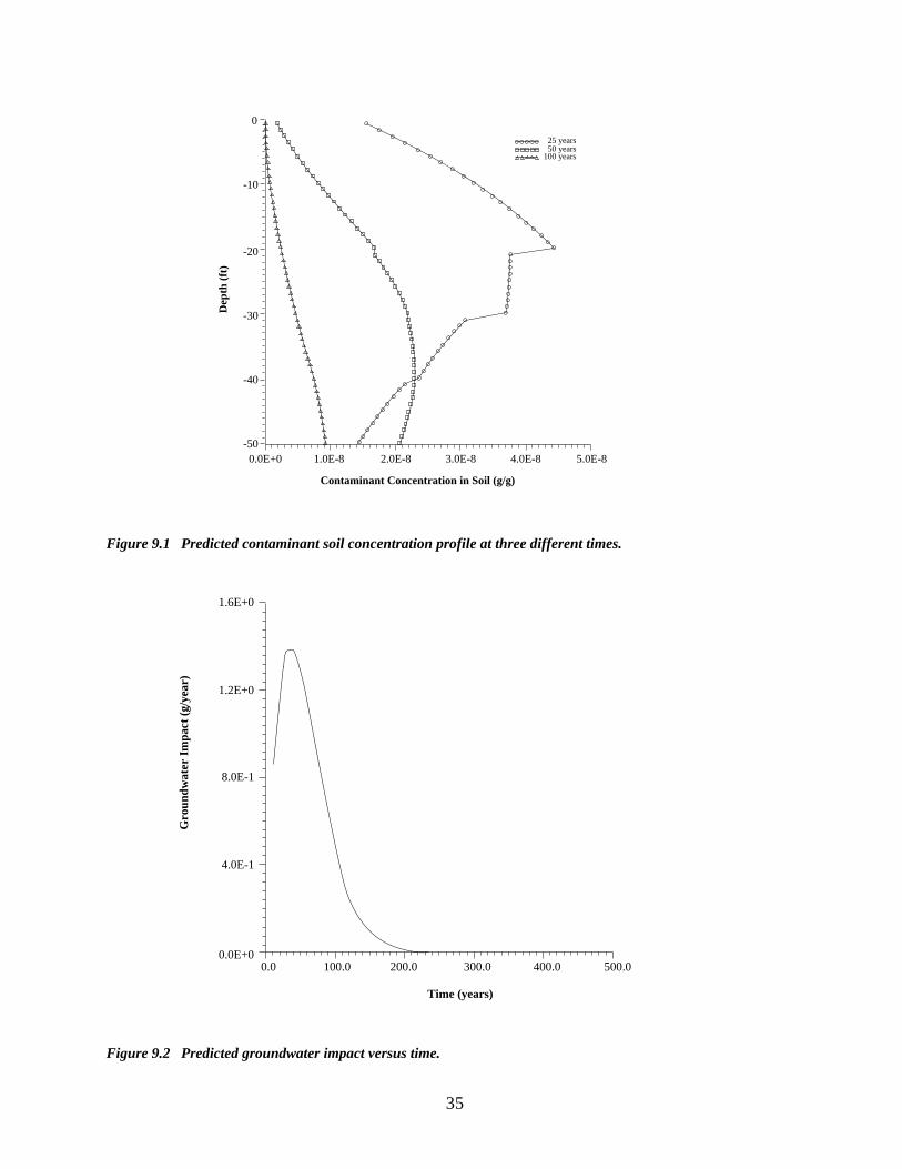
Figure 9.1 presents the concentration profile of TCE in soil for three different time values. The TCE level in the soil decreases from 4.5E-08 to 1.0E-0.8 with time due to leaching and volatilization. In addition the concentration of TCE becomes more evenly distributed with time. Figure 9.2 depicts the mass rate of TCE loading to groundwater as a function of time. The peak impact is approximately 1.4 g/year, and it occurs at about 50 years into the simulation.
34
0
-10
-20
-30
-40
-50
Dep
th (
ft)
25 years 50 years
100 years
0.0E+0 1.0E-8 2.0E-8 3.0E-8 4.0E-8 5.0E-8
Contaminant Concentration in Soil (g/g)
Figure 9.1 Predicted contaminant soil concentration profile at three different times.
0.0E+0 0.0 100.0 200.0 300.0 400.0
Gro
undw
ater
Im
pact
(g/
year
)
500.0
4.0E-1
8.0E-1
1.2E+0
1.6E+0
Time (years)
Figure 9.2 Predicted groundwater impact versus time.
35

36
10.0 REFERENCES
Bird, R., W.E. Stewart, and E.N. Lightfoot (1960), Transport Phenomena, John Wiley & Sons, Inc., NY.
Carsel, R.F. and R.S. Parrish (1988), “Variation within Texture Classes of Soil Water Characteristics,” Water Res. Research. vol. 24, pp. 755-769.
Dragun, J. (1988), The Soil Chemistry of Hazardous Materials, Hazardous Materials Control Research Institute, Silver Spring, MD.
Jury, W.A. (1986), in Vadose Zone Modeling of Organic Pollutants, Chapter 11, eds. S.C. Hern and S.M. Melancon, Lewis Publishers, Chelsea, MI.
Li, E.A., V.O. Shanholtz, and E.W. Carson (1976), Estimating Saturated Hydraulic Conductivity and Capillary Potential at the Wetting Front, Department of Agricultural Engineers, Virginia Polytechnic Institute and State University, Blacksburg.
McCuen, R.H., W.J. Rawls, and D.L. Brakensiek (1981), “Statistical Analysis of the Brooks-Corey and the Green-Ampt Parameter Across Soil Textures,” Water Resources Research, vol. 17, no. 4, pp. 1005-1013.
Rawls, W.J. (1983), “Estimating Bulk Density from Particle Size Analysis and Organic Matter Content,” Soil Science, vol. 135, no. 2, pp. 123-125.
Rosenbloom, J., P.Mock, P. Lawson, J. Brown, and H.J. Turin (1993) Application of VLEACH to Vadose Zone Transport of VOCs at an Arizona Superfund Site,”Ground Water Monitoring and Remediation, vol. 13, no.3, pp.159-169.
USEPA, (1990) Subsurface Contamination Reference Guide, Office of Emergency and Remedial Response, EPA/540/2-90/011.
37

38
APPENDIX A
SIMULATION PARAMETER INFORMATION

40
CHEMICAL
Properties of Volatile and Semi-Volatile Compounds
GROUP TYPE SOLUBILITY HENRY'S HENRY'S CONSTANT CONSTANT
(mg/l) (atm m3/mol) (dimensionless)
DENSITY
(g/cc)
LOG Kow LOG Koc
(cc/g)
Carbon Tetrachloride Chlorobenzene Chloroform Cis-1,2-dichloroethylene(d) 1,1-Dichloroethane(a) 1,2-Dichloroethane 1,1-Dichloroethylene 1,2-Dichloropropane(a) Ethylene Dibromide(g) Methylene Chloride 1,1,2,2-Tetrachloroethane Tetrachloroethylene Trans-1,2-dichloroethylene(d) 1,1,1-Trichloroethane 1,1,2-Trichloroethane Trichloroethylene Chloroethane Vinyl Chloride Methyl Ethyl Ketone 4-Methyl-2-Pentanone Tetrahydrofuran Benzene Ethyl Benzene Styrene Toluene m-Xylene o-Xylene p-Xylene Arochlor 1242 Arochlor 1254 Arochlor 1260 Chlordane DDD DDE DDT Dieldrin 1,2 Dichlorobenzene 1,4 Dichlorobenzene
Halogenated Volatile Organic Liquid Solvent 8.00E+02 2.00E-02 8.13E-01 Halogenated Volatile Organic Liquid Solvent 4.90E+02 3.46E-03 1.41E-01 Halogenated Volatile Organic Liquid Solvent 8.22E+03 3.75E-03 1.52E-01 Halogenated Volatile Organic Liquid Solvent 3.50E+03 7.50E-03 3.05E-01 Halogenated Volatile Organic Liquid Solvent 5.50E+03 5.70E-03 2.32E-01 Halogenated Volatile Organic Liquid Solvent 8.69E+03 1.10E-03 4.47E-02 Halogenated Volatile Organic Liquid Solvent 4.00E+02 1.54E-01 6.26E+00 Halogenated Volatile Organic Liquid Solvent 2.70E+03 3.60E-03 1.46E-01 Halogenated Volatile Organic Liquid Solvent 3.40E+03 3.18E-04 1.29E-02 Halogenated Volatile Organic Liquid Solvent 1.32E+04 2.57E-03 1.04E-01 Halogenated Volatile Organic Liquid Solvent 2.90E+03 5.00E-04 2.03E-02 Halogenated Volatile Organic Liquid Solvent 1.50E+02 2.27E-02 9.23E-01 Halogenated Volatile Organic Liquid Solvent 6.30E+03 6.60E-03 2.68E-01 Halogenated Volatile Organic Liquid Solvent 9.50E+02 2.76E-03 1.12E-01 Halogenated Volatile Organic Liquid Solvent 4.50E+03 1.17E-03 4.76E-02 Halogenated Volatile Organic Liquid Solvent 1.00E+03 8.92E-03 3.63E-01 Halogenated Volatile Organic Gas 5.70E+03 1.10E-02 4.47E-01 Halogenated Volatile Organic Gas 1.10E+03 6.95E-01 2.83E+01
Non-Halogenated Volatile Organic Ketone/furan 2.68E+05 2.74E-05 1.11E-03 Non-Halogenated Volatile Organic Ketone/furan 1.90E+04 1.55E-04 6.30E-03 Non-Halogenated Volatile Organic Ketone/furan 3.00E+05 1.10E-04 4.47E-03 Non-Halogenated Volatile Organic Aromatic 1.78E+03 5.43E-03 2.21E-01 Non-Halogenated Volatile Organic Aromatic 1.52E+02 7.90E-03 3.21E-01 Non-Halogenated Volatile Organic Aromatic 3.00E+02 2.28E-03 9.27E-02 Non-Halogenated Volatile Organic Aromatic 5.15E+02 6.61E-03 2.69E-01 Non-Halogenated Volatile Organic Aromatic 2.00E+02 6.91E-03 2.81E-01 Non-Halogenated Volatile Organic Aromatic 1.70E+02 4.94E-03 2.01E-01 Non-Halogenated Volatile Organic Aromatic 1.98E+02 7.01E-03 2.85E-01 Halogenated Semi-volatile Organic PCB 4.50E-01 3.40E-04 1.38E-02 Halogenated Semi-volatile Organic PCB 1.20E-02 2.80E-04 1.14E-02 Halogenated Semi-volatile Organic PCB 2.70E-03 3.40E-04 1.38E-02 Halogenated Semi-volatile Organic Pesticide 5.60E-02 2.20E-04 8.94E-03 Halogenated Semi-volatile Organic Pesticide 1.60E-01 7.96E-06 3.24E-04 Halogenated Semi-volatile Organic Pesticide 4.00E-02 1.90E-04 7.72E-03 Halogenated Semi-volatile Organic Pesticide 3.10E-03 2.80E-05 1.14E-03 Halogenated Semi-volatile Organic Pesticide 1.86E-01 9.70E-06 3.94E-04 Halogenated Semi-volatile Organic Chlorinated Benzene 1.00E+02 1.88E-03 7.64E-02 Halogenated Semi-volatile Organic Chlorinated Benzene 8.00E+01 1.58E-03 6.42E-02
1.595 1.106 1.485 1.284 1.175 1.253 1.214 1.158 2.172 1.325 1.600 1.625 1.257 1.325 1.444 1.462 0.941 0.912 0.805 0.802 0.889 0.877 0.867 0.906 0.867 0.864 0.880 0.861 1.385 1.538 1.440 1.600 1.385
no data 0.985 1.750 1.306 1.248
2.83 2.84 1.97 1.86 1.79 1.48 2.13 2.02 1.76 1.25 2.39 3.14 2.09 2.49 2.17 2.42 1.43 0.60 0.29 1.25 0.46 2.13 3.15 3.16 2.73 3.20 3.12 3.15 5.58 6.03 7.15 5.48 5.56 5.69 6.36 5.34 3.38 3.39
2.64 2.20 1.64 1.50 1.48 1.15 1.81 1.71 1.45 0.94 2.34 2.82 1.77 2.18 1.75 2.10 1.17 0.91 0.65 1.38
no data 1.81 2.83
no data 2.41 2.84 2.84 2.84 5.00
no data no data
4.58 5.38 5.41 5.48 3.23 3.06 3.07
A-1
CHEMICAL
Properties of Volatile and Semi-Volatile Compounds (continued)
GROUP TYPE SOLUBILITY HENRY'S HENRY'S DENSITY CONSTANT CONSTANT
(mg/l) (atm m3/mol) (dimensionless) (g/cc)
LOG Kow LOG Koc
(cc/g)
Pentachlorophenol(w) 2,3,4,6-Tetrachlorophenol Acenaphthene Anthracene Benzo(a)anthracene Benzo(a)pyrene Benzo(b)fluoranthene Benzo(ghi)perylene Benzo(k)fluoranthene Chrysene Dibenz(a,h)anthracene Fluoanthene Fluorene Indeno(1,2,3-cd)pyrene 2-Methyl Naphthalene Napthalene Phenanthrene Pyrene Phenol 2,4-Dinitrophenol m-Cresol (e) o-Cresol p-Cresol
Halogenated Semi-volatile Organic Chlorinated Phenol 1.40E+01 2.80E-06 1.14E-04 1.978 Halogenated Semi-volatile Organic Chorinated Phenol 1.00E+03 no data no data 1.839
Non-Halogenated Semi-volatile Organic PAH 3.88E+00 1.20E-03 4.88E-02 1.225 Non-Halogenated Semi-volatile Organic PAH 7.50E-02 3.38E-05 1.37E-03 1.250 Non-Halogenated Semi-volatile Organic PAH 1.40E-02 4.50E-06 1.83E-04 1.174 Non-Halogenated Semi-volatile Organic PAH 3.80E-03 1.80E-05 7.32E-04 no data Non-Halogenated Semi-volatile Organic PAH 1.40E-02 1.19E-05 4.84E-04 no data Non-Halogenated Semi-volatile Organic PAH 2.60E-04 5.34E-08 2.17E-06 no data Non-Halogenated Semi-volatile Organic PAH 4.30E-03 3.94E-05 1.60E-03 no data Non-Halogenated Semi-volatile Organic PAH 6.00E-03 1.05E-06 4.27E-05 1.274 Non-Halogenated Semi-volatile Organic PAH 2.50E-03 7 33E-08 2.98E-06 1.252 Non-Halogenated Semi-volatile Organic PAH 2.65E-01 6.50E-06 2.64E-04 1.252 Non-Halogenated Semi-volatile Organic PAH 1.90E+00 7.65E-05 3.11E-03 1.203 Non-Halogenated Semi-volatile Organic PAH 5.30E-04 6.95E-08 2.83E-06 no data Non-Halogenated Semi-volatile Organic PAH 2.54E+01 5.06E-02 2.06E+00 1.006 Non-Halogenated Semi-volatile Organic PAH 3.10E+01 1.27E-03 5.16E-02 1.162 Non-Halogenated Semi-volatile Organic PAH 1.18E+00 3.98E-05 1.62E-03 0.980 Non-Halogenated Semi-volatile Organic PAH 1.48E-01 1.20E-05 4.88E-04 1.271 Non-Halogenated Semi-volatile Organic Non-chlorinated phenol 8.40E+04 7.80E-07 3.17E-05 1.058 Non-Halogenated Semi-volatile Organic Non-chlorinated phenol 6.00E+03 6.50E-10 2.64E-08 1.680 Non-Halogenated Semi-volatile Organic Non-chlorinated phenol 2.35E+04 3.80E-05 1.54E-03 1.038 Non-Halogenated Semi-volatile Organic Non-chlorinated phenol 3.10E+04 4.70E-05 1.91E-03 1.027 Non-Halogenated Semi-volatile Organic Non-chlorinated phenol 2.40E+04 3.50E-04 1.42E-02 1.035
5.12 4.10 3.92 4.45 5.61 6.06 6.57 6.51 6.06 5.61 6.80 4.90 4.18 6.50 3.86 3.30 4.46 4.88 1.46 1.54 1.96 1.95 1.94
4.80 2.00 3.70 4.10 6.14 6.74 5.74 6.20 5.74 5.30 6.52 4.58 3.90 6.20 3.93 3.11 4.10 4.58 1.15 1.22 1.43 1.23 1.28
A-2
APPENDIX B
POLYGON PARAMETER INFORMATION

44
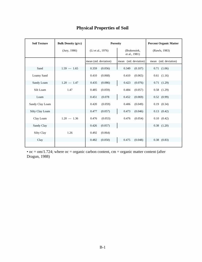
Physical Properties of Soil
Soil Texture Bulk Density (g/cc) Porosity Percent Organic Matter
(Jury, 1986) (Li et al., 1976) (Brakensiek, (Rawls, 1983) et al., 1981)
mean (std. deviation) mean (std. deviation) mean (std. deviation)
Sand 1.59 — 1.65 0.359 (0.056) 0.349 (0.107) 0.71 (1.06)
Loamy Sand 0.410 (0.068) 0.410 (0.065) 0.61 (1.16)
Sandy Loam 1.20 — 1.47 0.435 (0.086) 0.423 (0.076) 0.71 (1.29)
Silt Loam 1.47 0.485 (0.059) 0.484 (0.057) 0.58 (1.29)
Loam 0.451 (0.078 0.452 (0.069) 0.52 (0.99)
Sandy Clay Loam 0.420 (0.059) 0.406 (0.049) 0.19 (0.34)
Silty Clay Loam 0.477 (0.057) 0.473 (0.046) 0.13 (0.42)
Clay Loam 1.20 — 1.36 0.476 (0.053) 0.476 (0.054) 0.10 (0.42)
Sandy Clay 0.426 (0.057) 0.38 (1.20)
Silty Clay 1.26 0.492 (0.064)
Clay 0.482 (0.050) 0.475 (0.048) 0.38 (0.83)
• oc = om/1.724; where oc = organic carbon content, cm = organic matter content (after Dragun, 1988)
B-1
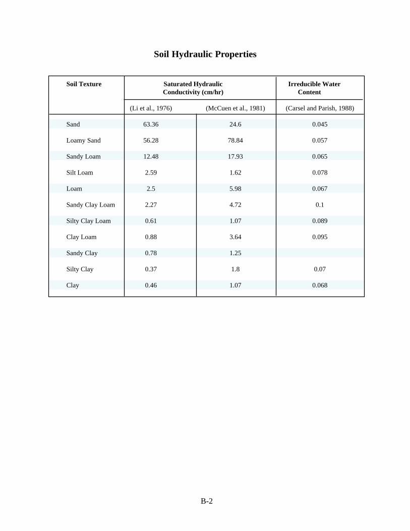
Soil Hydraulic Properties
Soil Texture Saturated HydraulicConductivity (cm/hr)
Irreducible Water Content
(Li et al., 1976) (McCuen et al., 1981) (Carsel and Parish, 1988)
Sand 63.36 24.6 0.045
Loamy Sand 56.28 78.84 0.057
Sandy Loam 12.48 17.93 0.065
Silt Loam 2.59 1.62 0.078
Loam 2.5 5.98 0.067
Sandy Clay Loam 2.27 4.72 0.1
Silty Clay Loam 0.61 1.07 0.089
Clay Loam 0.88 3.64 0.095
Sandy Clay 0.78 1.25
Silty Clay 0.37 1.8 0.07
Clay 0.46 1.07 0.068
B-2
APPENDIX C
REFERENCE INFORMATION

48
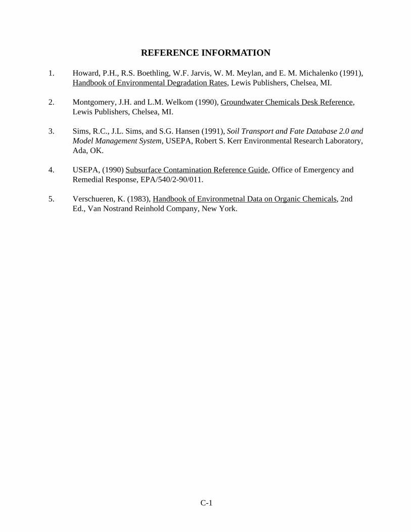
REFERENCE INFORMATION
1. Howard, P.H., R.S. Boethling, W.F. Jarvis, W. M. Meylan, and E. M. Michalenko (1991), Handbook of Environmental Degradation Rates, Lewis Publishers, Chelsea, MI.
2. Montgomery, J.H. and L.M. Welkom (1990), Groundwater Chemicals Desk Reference, Lewis Publishers, Chelsea, MI.
3. Sims, R.C., J.L. Sims, and S.G. Hansen (1991), Soil Transport and Fate Database 2.0 and Model Management System, USEPA, Robert S. Kerr Environmental Research Laboratory, Ada, OK.
4. USEPA, (1990) Subsurface Contamination Reference Guide, Office of Emergency and Remedial Response, EPA/540/2-90/011.
5. Verschueren, K. (1983), Handbook of Environmetnal Data on Organic Chemicals, 2nd Ed., Van Nostrand Reinhold Company, New York.
C-1
APPENDIX D
OUTPUT RESULTS FROM THE SAMPLE PROBLEM
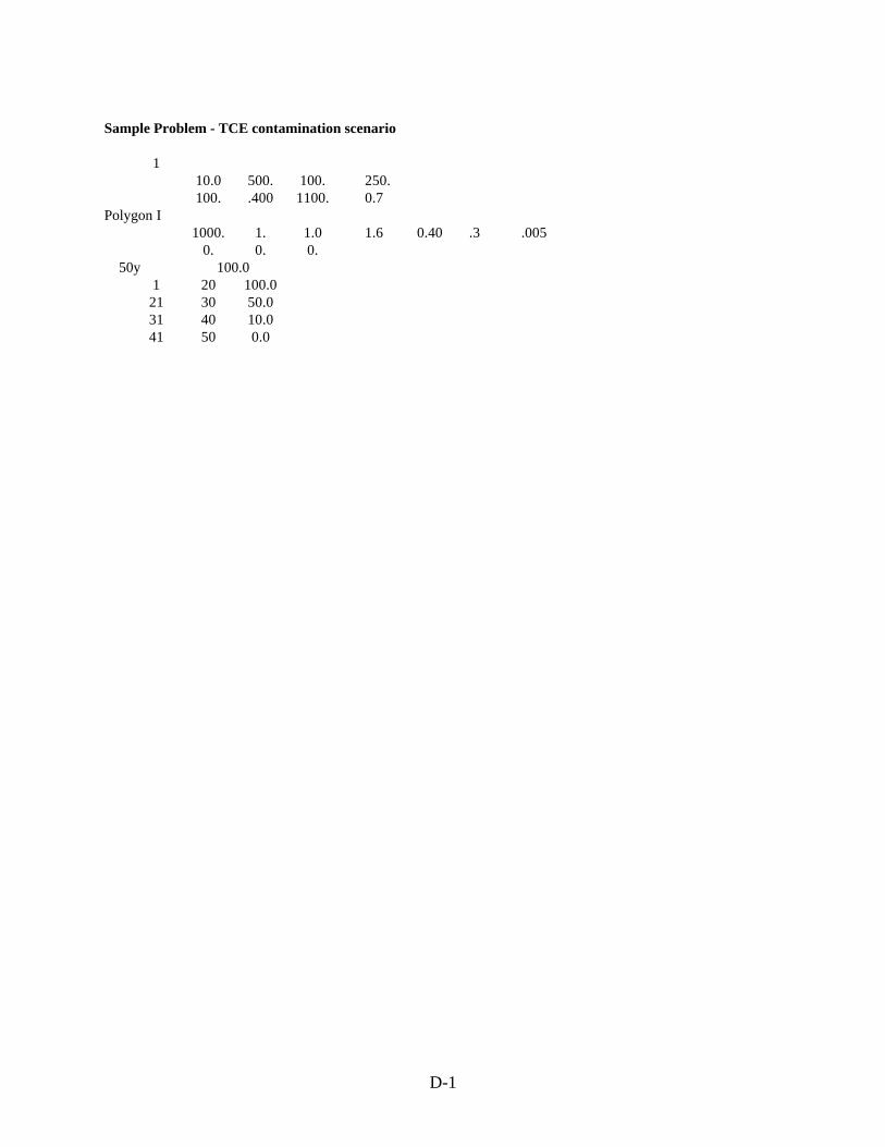
Sample Problem - TCE contamination scenario
1 10.0 500. 100. 250. 100. .400 1100. 0.7
Polygon I 1000. 1. 1.0 1.6 0.40 .3 .005
0. 0. 0. 50y 100.0
1 20 100.0 21 30 50.0 31 40 10.0 41 50 0.0
D-1
VLEACH Version 2.2a, 1996
By: Varadhan Ravi and Jeffrey A. Johnson
(USEPA Contractors) Center for Subsurface Modeling Support
Robert S. Kerr Environmental Research Laboratory U.S. Environmental Protection Agency
P.O. Box 1198 Ada, OK 74820
Based on the original VLEACH (version 1.0) developed by CH2M Hill, Redding, California for USEPA Region IX
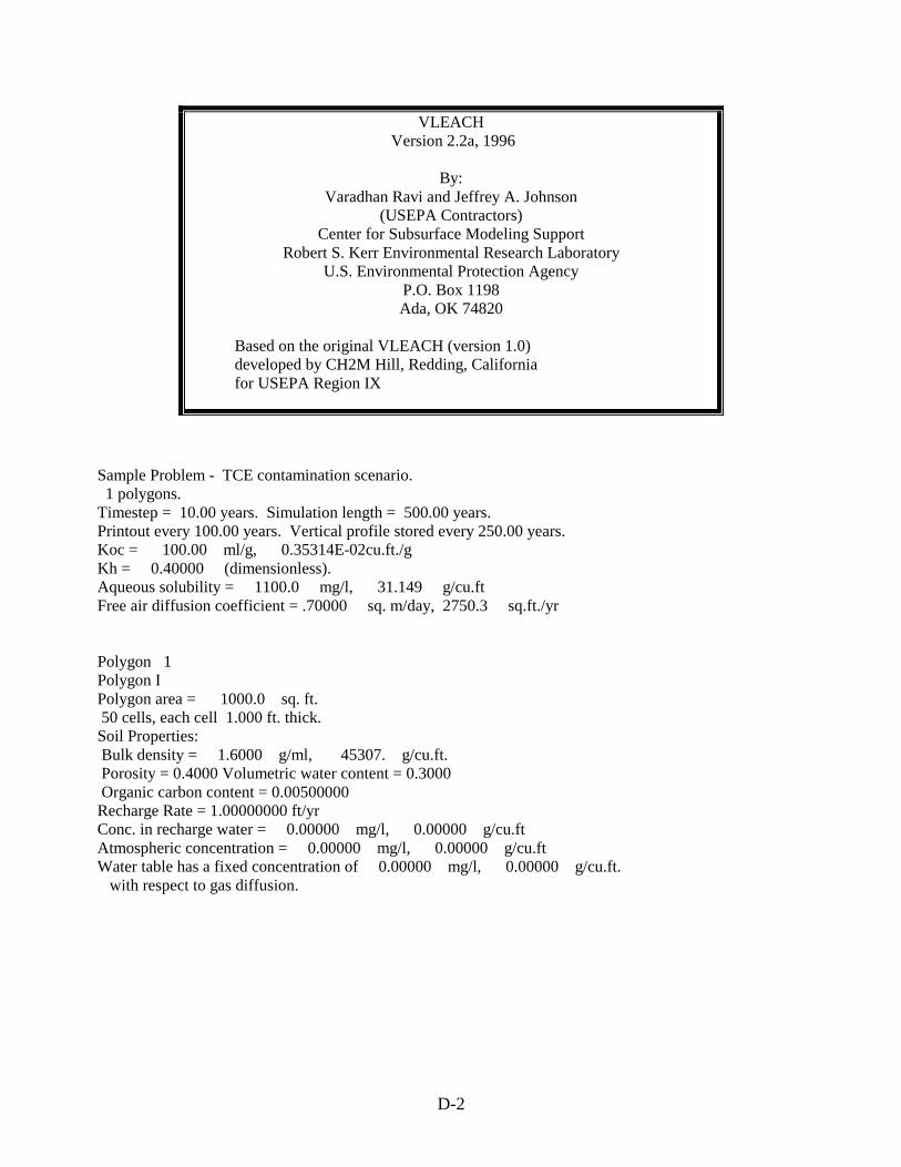
Sample Problem - TCE contamination scenario. 1 polygons. Timestep = 10.00 years. Simulation length = 500.00 years. Printout every 100.00 years. Vertical profile stored every 250.00 years. Koc = 100.00 ml/g, 0.35314E-02cu.ft./g Kh = 0.40000 (dimensionless). Aqueous solubility = 1100.0 mg/l, 31.149 g/cu.ft Free air diffusion coefficient = .70000 sq. m/day, 2750.3 sq.ft./yr
Polygon 1 Polygon I Polygon area = 1000.0 sq. ft. 50 cells, each cell 1.000 ft. thick.
Soil Properties: Bulk density = 1.6000 g/ml, 45307. g/cu.ft. Porosity = 0.4000 Volumetric water content = 0.3000 Organic carbon content = 0.00500000 Recharge Rate = 1.00000000 ft/yr Conc. in recharge water = 0.00000 mg/l, 0.00000 g/cu.ft Atmospheric concentration = 0.00000 mg/l, 0.00000 g/cu.ft Water table has a fixed concentration of 0.00000 mg/l, 0.00000 g/cu.ft. with respect to gas diffusion.
D-2
VLEACH Version 2.2a, 1996
By: Varadhan Ravi and Jeffrey A. Johnson
(USEPA Contractors) Center for Subsurface Modeling Support
Robert S. Kerr Environmental Research Laboratory U.S. Environmental Protection Agency
P.O. Box 1198 Ada, OK 74820
Based on the original VLEACH (version 1.0) developed by CH2M Hill, Redding, California for USEPA Region IX
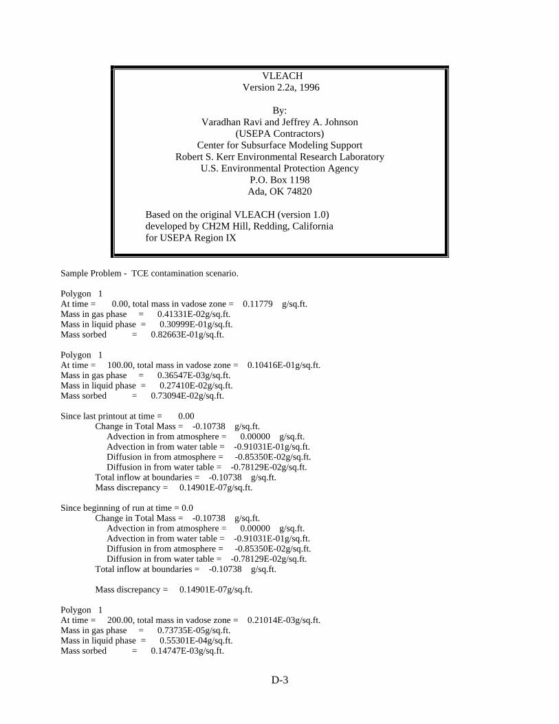
Sample Problem - TCE contamination scenario.
Polygon 1 At time = 0.00, total mass in vadose zone = 0.11779 g/sq.ft. Mass in gas phase = 0.41331E-02g/sq.ft. Mass in liquid phase = 0.30999E-01g/sq.ft. Mass sorbed = 0.82663E-01g/sq.ft.
Polygon 1 At time = 100.00, total mass in vadose zone = 0.10416E-01g/sq.ft. Mass in gas phase = 0.36547E-03g/sq.ft. Mass in liquid phase = 0.27410E-02g/sq.ft. Mass sorbed = 0.73094E-02g/sq.ft.
Since last printout at time = 0.00 Change in Total Mass = -0.10738 g/sq.ft. Advection in from atmosphere = 0.00000 g/sq.ft. Advection in from water table = -0.91031E-01g/sq.ft. Diffusion in from atmosphere = -0.85350E-02g/sq.ft. Diffusion in from water table = -0.78129E-02g/sq.ft. Total inflow at boundaries = -0.10738 g/sq.ft. Mass discrepancy = 0.14901E-07g/sq.ft.
Since beginning of run at time = 0.0 Change in Total Mass = -0.10738 g/sq.ft. Advection in from atmosphere = 0.00000 g/sq.ft. Advection in from water table = -0.91031E-01g/sq.ft. Diffusion in from atmosphere = -0.85350E-02g/sq.ft. Diffusion in from water table = -0.78129E-02g/sq.ft. Total inflow at boundaries = -0.10738 g/sq.ft.
Mass discrepancy = 0.14901E-07g/sq.ft.
Polygon 1 At time = 200.00, total mass in vadose zone = 0.21014E-03g/sq.ft. Mass in gas phase = 0.73735E-05g/sq.ft. Mass in liquid phase = 0.55301E-04g/sq.ft. Mass sorbed = 0.14747E-03g/sq.ft.
D-3
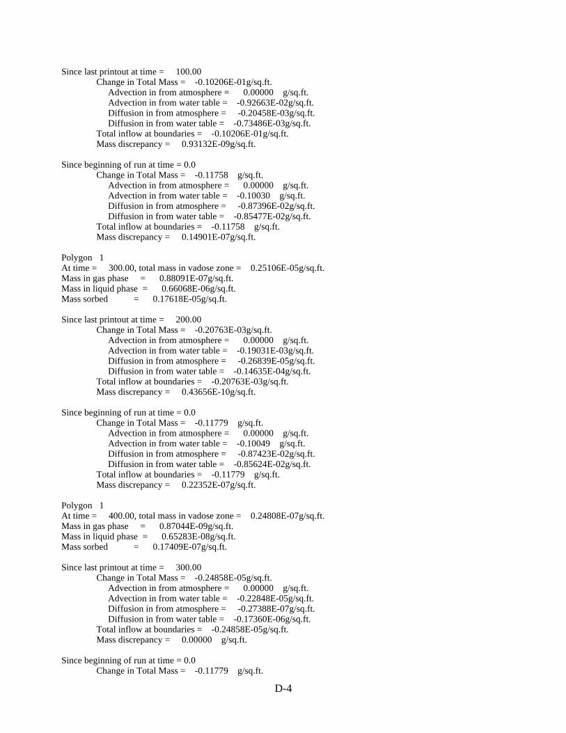
Since last printout at time = 100.00 Change in Total Mass = -0.10206E-01g/sq.ft. Advection in from atmosphere = 0.00000 g/sq.ft. Advection in from water table = -0.92663E-02g/sq.ft. Diffusion in from atmosphere = -0.20458E-03g/sq.ft. Diffusion in from water table = -0.73486E-03g/sq.ft. Total inflow at boundaries = -0.10206E-01g/sq.ft. Mass discrepancy = 0.93132E-09g/sq.ft.
Since beginning of run at time = 0.0 Change in Total Mass = -0.11758 g/sq.ft. Advection in from atmosphere = 0.00000 g/sq.ft. Advection in from water table = -0.10030 g/sq.ft. Diffusion in from atmosphere = -0.87396E-02g/sq.ft. Diffusion in from water table = -0.85477E-02g/sq.ft. Total inflow at boundaries = -0.11758 g/sq.ft. Mass discrepancy = 0.14901E-07g/sq.ft.
Polygon 1 At time = 300.00, total mass in vadose zone = 0.25106E-05g/sq.ft. Mass in gas phase = 0.88091E-07g/sq.ft. Mass in liquid phase = 0.66068E-06g/sq.ft. Mass sorbed = 0.17618E-05g/sq.ft.
Since last printout at time = 200.00 Change in Total Mass = -0.20763E-03g/sq.ft. Advection in from atmosphere = 0.00000 g/sq.ft. Advection in from water table = -0.19031E-03g/sq.ft. Diffusion in from atmosphere = -0.26839E-05g/sq.ft. Diffusion in from water table = -0.14635E-04g/sq.ft. Total inflow at boundaries = -0.20763E-03g/sq.ft. Mass discrepancy = 0.43656E-10g/sq.ft.
Since beginning of run at time = 0.0 Change in Total Mass = -0.11779 g/sq.ft. Advection in from atmosphere = 0.00000 g/sq.ft. Advection in from water table = -0.10049 g/sq.ft. Diffusion in from atmosphere = -0.87423E-02g/sq.ft. Diffusion in from water table = -0.85624E-02g/sq.ft. Total inflow at boundaries = -0.11779 g/sq.ft. Mass discrepancy = 0.22352E-07g/sq.ft.
Polygon 1 At time = 400.00, total mass in vadose zone = 0.24808E-07g/sq.ft. Mass in gas phase = 0.87044E-09g/sq.ft. Mass in liquid phase = 0.65283E-08g/sq.ft. Mass sorbed = 0.17409E-07g/sq.ft.
Since last printout at time = 300.00 Change in Total Mass = -0.24858E-05g/sq.ft. Advection in from atmosphere = 0.00000 g/sq.ft. Advection in from water table = -0.22848E-05g/sq.ft. Diffusion in from atmosphere = -0.27388E-07g/sq.ft. Diffusion in from water table = -0.17360E-06g/sq.ft. Total inflow at boundaries = -0.24858E-05g/sq.ft. Mass discrepancy = 0.00000 g/sq.ft.
Since beginning of run at time = 0.0 Change in Total Mass = -0.11779 g/sq.ft.
D-4
Advection in from atmosphere = 0.00000 g/sq.ft. Advection in from water table = -0.10049 g/sq.ft. Diffusion in from atmosphere = -0.87423E-02g/sq.ft. Diffusion in from water table = -0.85625E-02g/sq.ft. Total inflow at boundaries = -0.11779 g/sq.ft. Mass discrepancy = 0.29802E-07g/sq.ft.
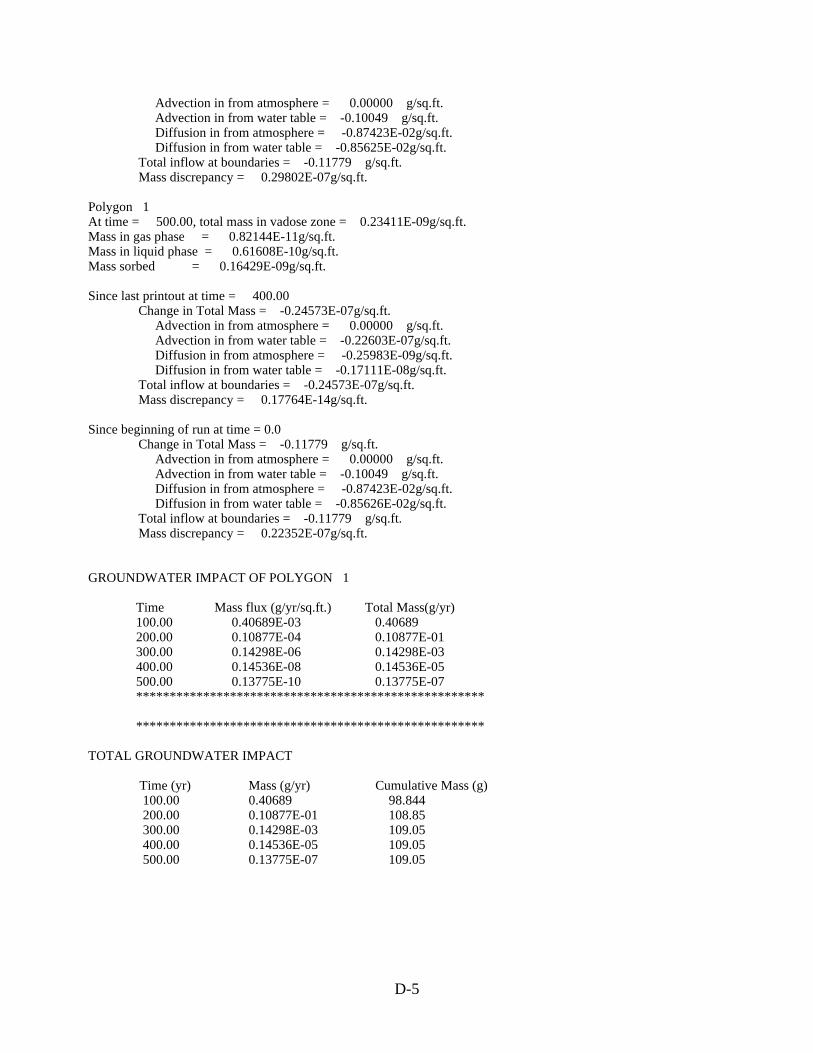
Polygon 1 At time = 500.00, total mass in vadose zone = 0.23411E-09g/sq.ft. Mass in gas phase = 0.82144E-11g/sq.ft. Mass in liquid phase = 0.61608E-10g/sq.ft. Mass sorbed = 0.16429E-09g/sq.ft.
Since last printout at time = 400.00 Change in Total Mass = -0.24573E-07g/sq.ft. Advection in from atmosphere = 0.00000 g/sq.ft. Advection in from water table = -0.22603E-07g/sq.ft. Diffusion in from atmosphere = -0.25983E-09g/sq.ft. Diffusion in from water table = -0.17111E-08g/sq.ft. Total inflow at boundaries = -0.24573E-07g/sq.ft. Mass discrepancy = 0.17764E-14g/sq.ft.
Since beginning of run at time = 0.0 Change in Total Mass = -0.11779 g/sq.ft. Advection in from atmosphere = 0.00000 g/sq.ft. Advection in from water table = -0.10049 g/sq.ft. Diffusion in from atmosphere = -0.87423E-02g/sq.ft. Diffusion in from water table = -0.85626E-02g/sq.ft. Total inflow at boundaries = -0.11779 g/sq.ft. Mass discrepancy = 0.22352E-07g/sq.ft.
GROUNDWATER IMPACT OF POLYGON 1
Time Mass flux (g/yr/sq.ft.) Total Mass(g/yr) 100.00 0.40689E-03 0.40689 200.00 0.10877E-04 0.10877E-01 300.00 0.14298E-06 0.14298E-03 400.00 0.14536E-08 0.14536E-05 500.00 0.13775E-10 0.13775E-07 ****************************************************
****************************************************
TOTAL GROUNDWATER IMPACT
Time (yr) Mass (g/yr) Cumulative Mass (g) 100.00 0.40689 98.844 200.00 0.10877E-01 108.85 300.00 0.14298E-03 109.05 400.00 0.14536E-05 109.05 500.00 0.13775E-07 109.05
D-5
�
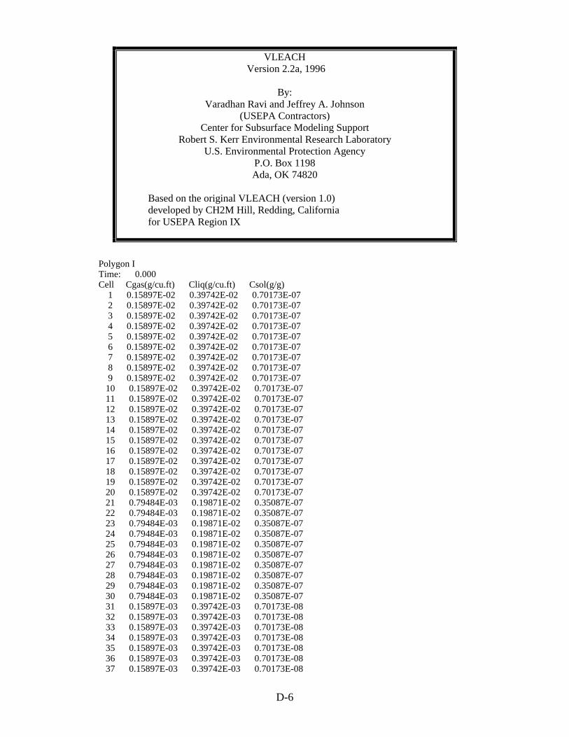
VLEACH Version 2.2a, 1996
By: Varadhan Ravi and Jeffrey A. Johnson
(USEPA Contractors) Center for Subsurface Modeling Support
Robert S. Kerr Environmental Research Laboratory U.S. Environmental Protection Agency
P.O. Box 1198 Ada, OK 74820
Based on the original VLEACH (version 1.0) developed by CH2M Hill, Redding, California for USEPA Region IX
Polygon I Time: 0.000 Cell Cgas(g/cu.ft) Cliq(g/cu.ft) Csol(g/g)
1 0.15897E-02 0.39742E-02 0.70173E-07 2 0.15897E-02 0.39742E-02 0.70173E-07 3 0.15897E-02 0.39742E-02 0.70173E-07 4 0.15897E-02 0.39742E-02 0.70173E-07 5 0.15897E-02 0.39742E-02 0.70173E-07 6 0.15897E-02 0.39742E-02 0.70173E-07 7 0.15897E-02 0.39742E-02 0.70173E-07 8 0.15897E-02 0.39742E-02 0.70173E-07 9 0.15897E-02 0.39742E-02 0.70173E-07
10 0.15897E-02 0.39742E-02 0.70173E-07 11 0.15897E-02 0.39742E-02 0.70173E-07 12 0.15897E-02 0.39742E-02 0.70173E-07 13 0.15897E-02 0.39742E-02 0.70173E-07 14 0.15897E-02 0.39742E-02 0.70173E-07 15 0.15897E-02 0.39742E-02 0.70173E-07 16 0.15897E-02 0.39742E-02 0.70173E-07 17 0.15897E-02 0.39742E-02 0.70173E-07 18 0.15897E-02 0.39742E-02 0.70173E-07 19 0.15897E-02 0.39742E-02 0.70173E-07 20 0.15897E-02 0.39742E-02 0.70173E-07 21 0.79484E-03 0.19871E-02 0.35087E-07 22 0.79484E-03 0.19871E-02 0.35087E-07 23 0.79484E-03 0.19871E-02 0.35087E-07 24 0.79484E-03 0.19871E-02 0.35087E-07 25 0.79484E-03 0.19871E-02 0.35087E-07 26 0.79484E-03 0.19871E-02 0.35087E-07 27 0.79484E-03 0.19871E-02 0.35087E-07 28 0.79484E-03 0.19871E-02 0.35087E-07 29 0.79484E-03 0.19871E-02 0.35087E-07 30 0.79484E-03 0.19871E-02 0.35087E-07 31 0.15897E-03 0.39742E-03 0.70173E-08 32 0.15897E-03 0.39742E-03 0.70173E-08 33 0.15897E-03 0.39742E-03 0.70173E-08 34 0.15897E-03 0.39742E-03 0.70173E-08 35 0.15897E-03 0.39742E-03 0.70173E-08 36 0.15897E-03 0.39742E-03 0.70173E-08 37 0.15897E-03 0.39742E-03 0.70173E-08
D-6
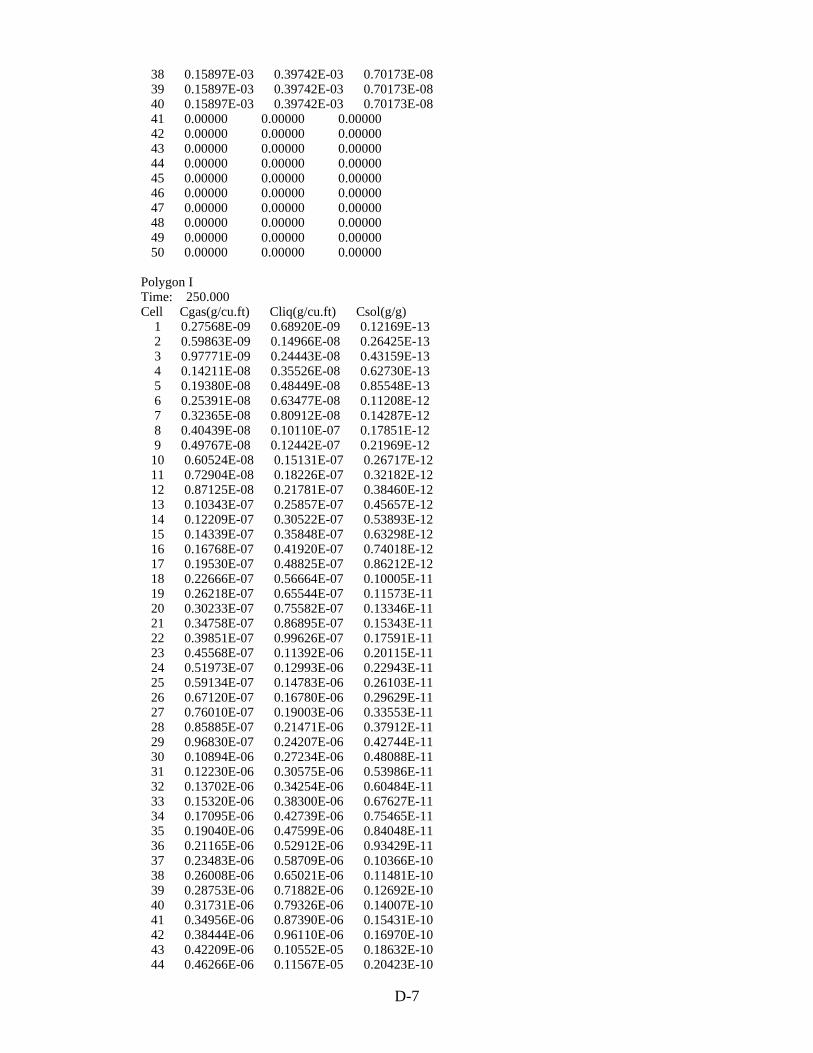
38 0.15897E-03 0.39742E-03 0.70173E-08 39 0.15897E-03 0.39742E-03 0.70173E-08 40 0.15897E-03 0.39742E-03 0.70173E-08 41 0.00000 0.00000 0.00000 42 0.00000 0.00000 0.00000 43 0.00000 0.00000 0.00000 44 0.00000 0.00000 0.00000 45 0.00000 0.00000 0.00000 46 0.00000 0.00000 0.00000 47 0.00000 0.00000 0.00000 48 0.00000 0.00000 0.00000 49 0.00000 0.00000 0.00000 50 0.00000 0.00000 0.00000
Polygon I Time: 250.000 Cell Cgas(g/cu.ft) Cliq(g/cu.ft) Csol(g/g)
1 0.27568E-09 0.68920E-09 0.12169E-13 2 0.59863E-09 0.14966E-08 0.26425E-13 3 0.97771E-09 0.24443E-08 0.43159E-13 4 0.14211E-08 0.35526E-08 0.62730E-13 5 0.19380E-08 0.48449E-08 0.85548E-13 6 0.25391E-08 0.63477E-08 0.11208E-12 7 0.32365E-08 0.80912E-08 0.14287E-12 8 0.40439E-08 0.10110E-07 0.17851E-12 9 0.49767E-08 0.12442E-07 0.21969E-12
10 0.60524E-08 0.15131E-07 0.26717E-12 11 0.72904E-08 0.18226E-07 0.32182E-12 12 0.87125E-08 0.21781E-07 0.38460E-12 13 0.10343E-07 0.25857E-07 0.45657E-12 14 0.12209E-07 0.30522E-07 0.53893E-12 15 0.14339E-07 0.35848E-07 0.63298E-12 16 0.16768E-07 0.41920E-07 0.74018E-12 17 0.19530E-07 0.48825E-07 0.86212E-12 18 0.22666E-07 0.56664E-07 0.10005E-11 19 0.26218E-07 0.65544E-07 0.11573E-11 20 0.30233E-07 0.75582E-07 0.13346E-11 21 0.34758E-07 0.86895E-07 0.15343E-11 22 0.39851E-07 0.99626E-07 0.17591E-11 23 0.45568E-07 0.11392E-06 0.20115E-11 24 0.51973E-07 0.12993E-06 0.22943E-11 25 0.59134E-07 0.14783E-06 0.26103E-11 26 0.67120E-07 0.16780E-06 0.29629E-11 27 0.76010E-07 0.19003E-06 0.33553E-11 28 0.85885E-07 0.21471E-06 0.37912E-11 29 0.96830E-07 0.24207E-06 0.42744E-11 30 0.10894E-06 0.27234E-06 0.48088E-11 31 0.12230E-06 0.30575E-06 0.53986E-11 32 0.13702E-06 0.34254E-06 0.60484E-11 33 0.15320E-06 0.38300E-06 0.67627E-11 34 0.17095E-06 0.42739E-06 0.75465E-11 35 0.19040E-06 0.47599E-06 0.84048E-11 36 0.21165E-06 0.52912E-06 0.93429E-11 37 0.23483E-06 0.58709E-06 0.10366E-10 38 0.26008E-06 0.65021E-06 0.11481E-10 39 0.28753E-06 0.71882E-06 0.12692E-10 40 0.31731E-06 0.79326E-06 0.14007E-10 41 0.34956E-06 0.87390E-06 0.15431E-10 42 0.38444E-06 0.96110E-06 0.16970E-10 43 0.42209E-06 0.10552E-05 0.18632E-10 44 0.46266E-06 0.11567E-05 0.20423E-10
D-7
45 0.50632E-06 0.12658E-05 0.22351E-10 46 0.55322E-06 0.13830E-05 0.24421E-10 47 0.60351E-06 0.15088E-05 0.26641E-10 48 0.65737E-06 0.16434E-05 0.29018E-10 49 0.71496E-06 0.17874E-05 0.31561E-10 50 0.77644E-06 0.19411E-05 0.34275E-10
Polygon I Time: 500.000 Cell Cgas(g/cu.ft) Cliq(g/cu.ft) Csol(g/g)
1 0.25482E-14 0.63705E-14 0.11248E-18 2 0.55496E-14 0.13874E-13 0.24498E-18 3 0.90611E-14 0.22653E-13 0.39998E-18 4 0.13146E-13 0.32866E-13 0.58032E-18 5 0.17876E-13 0.44691E-13 0.78911E-18 6 0.23331E-13 0.58327E-13 0.10299E-17 7 0.29599E-13 0.73997E-13 0.13066E-17 8 0.36780E-13 0.91949E-13 0.16236E-17 9 0.44985E-13 0.11246E-12 0.19858E-17
10 0.54338E-13 0.13585E-12 0.23987E-17 11 0.64979E-13 0.16245E-12 0.28684E-17 12 0.77064E-13 0.19266E-12 0.34018E-17 13 0.90764E-13 0.22691E-12 0.40066E-17 14 0.10628E-12 0.26569E-12 0.46914E-17 15 0.12382E-12 0.30954E-12 0.54656E-17 16 0.14363E-12 0.35907E-12 0.63401E-17 17 0.16598E-12 0.41495E-12 0.73268E-17 18 0.19118E-12 0.47794E-12 0.84391E-17 19 0.21956E-12 0.54890E-12 0.96921E-17 20 0.25151E-12 0.62877E-12 0.11102E-16 21 0.28745E-12 0.71862E-12 0.12689E-16 22 0.32786E-12 0.81964E-12 0.14473E-16 23 0.37326E-12 0.93315E-12 0.16477E-16 24 0.42426E-12 0.10606E-11 0.18728E-16 25 0.48151E-12 0.12038E-11 0.21255E-16 26 0.54577E-12 0.13644E-11 0.24092E-16 27 0.61787E-12 0.15447E-11 0.27275E-16 28 0.69874E-12 0.17469E-11 0.30845E-16 29 0.78943E-12 0.19736E-11 0.34848E-16 30 0.89109E-12 0.22277E-11 0.39336E-16 31 0.10050E-11 0.25126E-11 0.44365E-16 32 0.11327E-11 0.28318E-11 0.50002E-16 33 0.12758E-11 0.31894E-11 0.56316E-16 34 0.14360E-11 0.35900E-11 0.63389E-16 35 0.16154E-11 0.40386E-11 0.71310E-16 36 0.18163E-11 0.45408E-11 0.80178E-16 37 0.20412E-11 0.51030E-11 0.90105E-16 38 0.22929E-11 0.57322E-11 0.10121E-15 39 0.25744E-11 0.64361E-11 0.11364E-15 40 0.28894E-11 0.72235E-11 0.12755E-15 41 0.32416E-11 0.81040E-11 0.14309E-15 42 0.36354E-11 0.90884E-11 0.16048E-15 43 0.40754E-11 0.10188E-10 0.17990E-15 44 0.45670E-11 0.11418E-10 0.20160E-15 45 0.51161E-11 0.12790E-10 0.22584E-15 46 0.57290E-11 0.14323E-10 0.25290E-15 47 0.64131E-11 0.16033E-10 0.28309E-15 48 0.71761E-11 0.17940E-10 0.31678E-15 49 0.80269E-11 0.20067E-10 0.35433E-15 50 0.89750E-11 0.22438E-10 0.39619E-15�
D-8
APPENDIX E
MODEL DATA SHEET

62
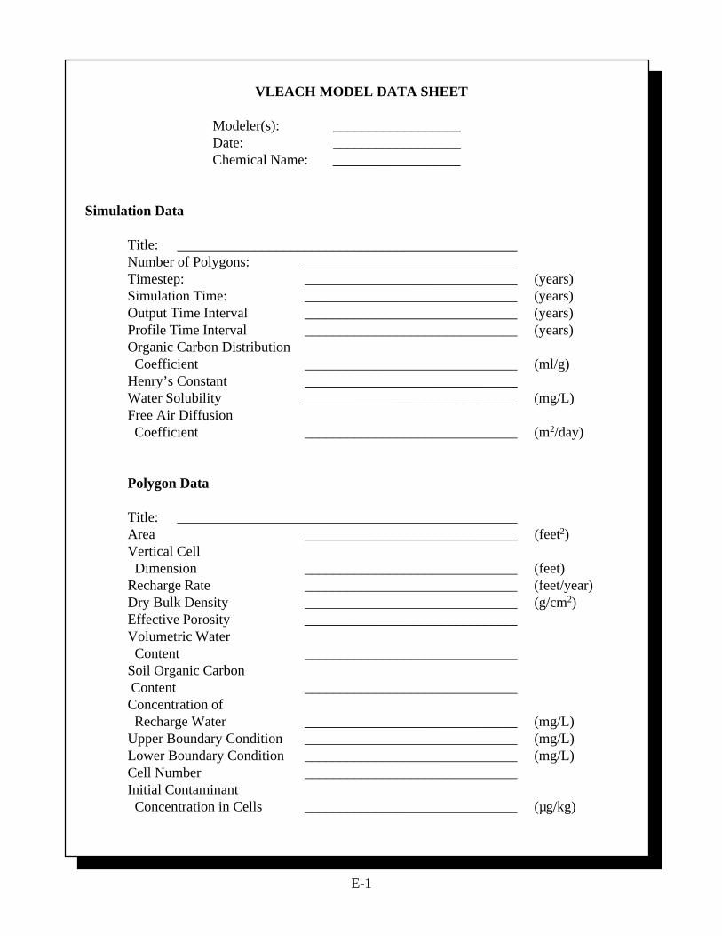
VLEACH MODEL DATA SHEET
Modeler(s): __________________ Date: __________________ Chemical Name: __________________
Simulation Data
Title: ________________________________________________ Number of Polygons: ______________________________ Timestep: ______________________________ (years) Simulation Time: ______________________________ (years) Output Time Interval ______________________________ (years) Profile Time Interval ______________________________ (years) Organic Carbon Distribution Coefficient ______________________________ (ml/g) Henry’s Constant ______________________________ Water Solubility ______________________________ (mg/L) Free Air Diffusion Coefficient ______________________________ (m2/day)
Polygon Data
Title: ________________________________________________ Area ______________________________ (feet2) Vertical Cell Dimension ______________________________ (feet)
Recharge Rate ______________________________ (feet/year) Dry Bulk Density ______________________________ (g/cm2) Effective Porosity ______________________________ Volumetric Water Content ______________________________ Soil Organic Carbon Content ______________________________ Concentration of Recharge Water ______________________________ (mg/L) Upper Boundary Condition ______________________________ (mg/L) Lower Boundary Condition ______________________________ (mg/L) Cell Number ______________________________ Initial Contaminant Concentration in Cells ______________________________ (µg/kg)
E-1