Vlajic, N., Champneys, A. R., & Balachandran, B. (2017). Nonlineardynamics of a Jeffcott rotor with torsional deformations and rotor-statorcontact. International Journal of Non-Linear Mechanics, 92, 102-110.https://doi.org/10.1016/j.ijnonlinmec.2017.02.002

Peer reviewed version

License (if available):CC BY-NC-ND

Link to published version (if available):10.1016/j.ijnonlinmec.2017.02.002

Link to publication record in Explore Bristol ResearchPDF-document

This is the author accepted manuscript (AAM). The final published version (version of record) is available onlinevia Elsevier at http://www.sciencedirect.com/science/article/pii/S0020746217300823?via%3Dihub. Please referto any applicable terms of use of the publisher.

University of Bristol - Explore Bristol ResearchGeneral rights

This document is made available in accordance with publisher policies. Please cite only the publishedversion using the reference above. Full terms of use are available:http://www.bristol.ac.uk/pure/about/ebr-terms

Nonlinear Dynamics of a Jeffcott Rotor with TorsionalDeformations and Rotor-Stator Contact

Nicholas Vlajica , Alan R. Champneysa , Balakumar Balachandranb

aDepartment of Engineering Mathematics, University of Bristol, Bristol, EnglandbDepartment of Mechanical Engineering, University of Maryland, College Park, USA

Abstract

The dynamics of a modified Jeffcott rotor is studied, including rotor torsional deformationand rotor-stator contact. Conditions are studied under which the rotor undergoes either forwardsynchronous whirling or self-excited backward whirling motions with continuous stator contact.For forward whirling, the effect on the response is investigated for two commonly used rotor-stator friction models, namely, the simple Coulomb friction and a generalised Coulomb law withcubic dependence on the relative slip velocity. For cases with and without the rotor torsionaldegree of freedom, analytical estimates and numerical bifurcation analyses are used to map outregions in the space of drive speed and a friction parameter, where rotor-stator contact exists.The nature of the bifurcations in which stability is lost are highlighted. For forward synchronouswhirling fold, Hopf, lift-off, and period-doubling bifurcations are encountered. Additionally,for backward whirling, regions of transitions from pure sticking to stick-slip oscillations arenumerically delineated.

Keywords: Jeffcott rotor, bifurcations, drill-string dynamics, nonlinear oscillations, torsionalvibrations

1. Introduction

The focus of this paper is on the dynamics of a modified version of the Jeffcott rotor [1], in-cluding the geometric nonlinearity originating from torsional-lateral coupling and friction due torotor-stator contact. Such a rotor, which can undergo elastic torsional deformations in addition tothe rigid body rotation about its drive axis has been studied previously, see [2] and the referenceswithin.

A key motivation for this simplified single-rotor model is its application in understanding thedynamics of rotary drill-strings, which are slender rotating structures that are used to drill forpetrochemicals and in other geothermal applications. These structures are rather different fromtypical rotating machines, because they typically have large torsional deformations and can alsofeature significant imbalance and eccentricity originating from curvature in the string. Moreover,rotor-stator contact is often designed to be a key part of such devices through the introduction ofstabilizing disks.

Previously, Edwards et al. [3] performed a parametric study of a rotor-stator system simi-lar to the one presented here and mapped out regions of impacting motions and quasi-periodicbehavior.

Preprint submitted to pick journal later March 16, 2017

A main contribution of prior work [2] was the construction of a reduced-order model to showhow the combined effects of lateral-torsional and nonlinear friction between the rotor and statorcould create a Hopf instability during forward synchronous whirl with stator contact. Further-more, an approximate analytic solution was derived in order to describe the torsional responseduring self-excited backward whirling vibrations for weakly nonlinear friction and for whirlspeeds much greater than the uncoupled torsional natural frequency. Finally, the prior work [2]did not consider conditions under which loss of contact might occur.

Key questions remain as to how the approximate solutions presented in [2] map out into widerparameter regimes and to what extent the stability map is sensitively dependent on the choice offriction model. In this paper, the prior work in [2] is extended to answer these questions, via amixture of analytical and numerical techniques. A more comprehensive study is performed toinvestigate the response of this rotor system during both forward and backward whirling withcontinuous stator contact. In particular, for typical sets of physical parameter values, we seekto map out the bifurcations that delineate regions of rotor-stator contact, synchronous forwardwhirl, self-excited backward whirl, and torsional oscillations with contact.

The work presented here is similar in spirit to the stability analysis performed by Miha-jlovic et al. [4] who used experiments and a numerical model of a rotating shaft that is able toundergo torsional motions, but is constrained laterally. There, all of the nonlinear phenomenaoriginated from the specific forms of the set-valued or velocity-weakening friction models, ratherthan through geometric effects. In a follow study [5], the same authors extended this model toinclude lateral deformations, but in which forces were assumed to be of follower-type and to acton the rotor for all lateral displacements. By contrast, in the model presented in Section 2 below,the authors do not make any such geometric approximations.

Using a similar model to the one presented here, it has been known at least since the workof Edwards et al. [3] that complex nonlinear motions can occur. In particular, they were able tomap out parameter regions of impacting motion and quasi-periodic behavior.

It should however be noted that lateral-torsional coupling is not a necessary ingredient forrotor systems to exhibit impacting, aperiodic, or chaotic motions; see for example [6, 7]. Severalstudies, including those by [8, 9], have been devoted to investigating the onset and mechanism ofself-excited backward whirl. Yet few studies [2, 10–12] have included torsional during analysisof backward whirling motions. Also, we are not aware of any previous presentation of a funda-mental diagram showing the existence regions of synchronous forward whirl (cf. Fig. 3 below),even in the absence of torsional effects.

The rest of this paper is outlined as follows. In Section 2, the governing equations of motions,which were originally derived in [2], are presented here for completeness. Section 3 containscomputations of existence and stability regions for the special case where there is no couplingbetween lateral and torsional motions. The cases of forward and backward whirl are consideredseperately. In Section 4, the additional effects induced by torsional coupling are pointed out.Finally, Section 5 includes concluding remarks.

2. Rotor Equations of Motion and External Stator Forces

2.1. Derivation of Equations of Motion

A schematic of the Jeffcott rotor-stator system capable of torsional vibrations is shown inFigure 1(a). The rotor with radius R and mass M coincides with the center of the stator with aclearance δ in the static configuration. The rotor has a mass imbalance m with eccentricity e.

2

The quantity Jo is the mass moment of inertia of the rotor without mass imbalance about the z-axis. The rotor is assumed to be symmetrical so that the lateral stiffnesses have equivalent springconstants kx = ky = kb, and has a torsional stiffness k. Similarly, the rotor has lateral dampingthat is assumed to be symmetric so that the equivalent damping coefficients are cx = cy = cb.Torsional motions also experience dissipation denoted by the damping coefficient c. A schematicof the rotor in a dynamic state at an instant of time is depicted in Figure 1(b). The geometriccenter of the planar rotor is fully described in an inertial frame with coordinates x and y projectedonto orthogonal unit vectors a1 and a2, respectively. Further, two sets of unit vectors, namelyb1,b2 and c1,c2, are placed at the geometric center of the rotor.

The b1-b2 set rotates at a constant angular speed Ω with respect to the a1-a2 set. Thus, theangle between a1 and b1 is a measure of the rigid body rotation which we assume to be equal toΩt, where Ω is an applied external drive frequency.

The mutually orthogonal unit vectors c1 and c2 are fixed to the rotor, and the angle betweenb1 and c1 is the torsional deformation given by θ. For notational convenience, let

β(t) ≡ β = θ(t) + Ωt,

which represents the superposition of the torsional deformation and rigid body rotation. Physi-cally, the torsional stiffness k and damping c act to align the b1,b2 and c1,c2 unit vectors.

Additionally, the rotor is assumed to be only able to undergo planar motions with no out ofplane motions due to rotations about the x and y axes. This constraint is imposed by defininga3 ≡ b3 ≡ c3 for all time t, where a3 ≡ a1 × a2, b3 ≡ b1 × b2 and c3 ≡ c1 × c2. For convenience,at time t = 0, we suppose that a1 ≡ b1 ≡ c1, a2 ≡ b2 ≡ c2 and the mass imbalance m is locatedalong the x-axis.

Under these assumptions, the equations of motion can readily be obtained by using La-grangian mechanics, see [2] for details:

(M + m) ¨x + cb ˙x + kb x = me[β sin β + β2 cos β

]+ Fx, (1)

(M + m)¨y + cb ˙y + kby = me[−β cos β + β2 sin β

]+ Fy, (2)

Jθ + cθ + kθ = me[ ¨x sin β − ¨y cos β

]+ Mt, (3)

in which J = Jo + me2. For analysis (but not simulations, because of the polar singularity) it isuseful to express the position of the rotor in polar coordinates. In light of this, Eqs. (1), (2), and(3) can be written in polar coordinates with the transformation

x = ρ cos γ (4a)y = ρ sin γ (4b)

In Eqs. (4), barρ ≡ ρ(t) is the polar amplitude and γ ≡ γ(t) is the angle between the positionvector from the origin to the geometric center of the rotor and the x-axis. In practice, it is simplerto substitute Eqs. (4) into the kinetic energy, potential, and Raleigh’s dissipation function givenin [2] and use Lagrange’s equations with generalized coordinates ρ, γ, and θ. Equations (1), (2),and (3) can then be re-written in polar coordinates as:

(M + m) ¨ρ − (M + m)ργ2 + cb ˙ρ + kbρ = me(Ω + θ

)2cosψ + meθ sinψ − Fn, (5)

3

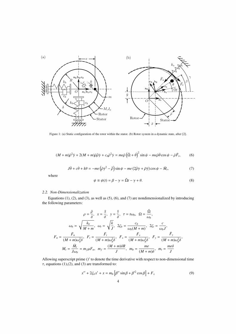
Figure 1: (a) Static configuration of the rotor within the stator. (b) Rotor system in a dynamic state, after [2].

(M + m)ρ2γ + 2(M + m)ρ ˙ργ + cbρ2γ = meρ

(Ω + θ

)2sinψ − meρθ cosψ − ρFt, (6)

Jθ + cθ + kθ = −me(ργ2 − ¨ρ

)sinψ − me

(2 ˙ργ + ργ

)cosψ − Mt, (7)

whereψ ≡ ψ(t) = β − γ = Ωt − γ + θ. (8)

2.2. Non-Dimensionalization

Equations (1), (2), and (3), as well as (5), (6), and (7) are nondimensionalized by introducingthe following parameters:

ρ =ρ

δ, x =

xδ, y =

yδ, τ = tωb, Ω =

Ω

ωb,

ωb =

√kb

M + m, ωt =

√kJ, 2ζb =

cb

ωb(M + m), 2ζt =

cωbJ

,

Fn =Fn

(M + m)ω2bδ, Ft =

Ft

(M + m)ω2bδ, Fx =

Fx

(M + m)ω2bδ, Fy =

Fy

(M + m)ω2bδ,

Mt =Mt

Jωb= m fµFn, m f =

(M + m)δRJ

, mb =me

(M + m)δ, mt =

meδJ

Allowing superscript prime ()′ to denote the time derivative with respect to non-dimensional timeτ, equations (1),(2), and (3) are transformed to:

x′′ + 2ζbx′ + x = mb

[β′′ sin β + β′2 cos β

]+ Fx (9)

4

y′′ + 2ζby′ + y = mb

[−β′′ cos β + β′2 sin β

]+ Fy (10)

θ′′ + 2ζtθ′ + ω2

t /ω2bθ = mt

[x′′ sin β − y′′ cos β

]+ Mt (11)

Similarly, equations (12), (13), and (14) are then rewritten:

ρ′′ − ργ′2 + 2ζbρ′ + ρ = mb(Ω + θ′)2 cosψ + mbθ

′′ sinψ − Fn (12)

ρ2γ′′ + 2ρρ′γ′ + 2ζbρ2γ′ = mbρ(Ω + θ′)2 sinψ − mbρθ

′′ cosψ − ρFt (13)

θ′′ + 2ζtθ′ + ω2

t /ω2bθ = −mt(ργ′2 − ρ′′) sinψ − mt(2ρ′γ′ + ργ′′) cosψ − Mt (14)

2.3. External Stator Forces

Upon contact with the stator, the rotor is subject to a normal force that is assumed to belinearly proportional to the deflection of the stator with stiffness ks. This may be written as

Fn =

0 for ρ ≤ δks(ρ − δ) for ρ > δ , (15)

where ks 1. The tangential force component is assumed to obey the usual principle of dryfriction and is proportional to the normal force and a friction coefficient µ, via

Ft = µFn.

The tangential and normal forces may be transformed to accommodate the external forcesand moments in Eqs. (9),(10) and (11) by using the following geometric relations

Fx =Fty − Fnx

ρ, Fy =

−Ft x − Fnyρ

, Mt = FtR for ρ , 0 (16)

2.4. Friction Models

The stability of the torsional vibrations and rotor response is studied for two different frictionmodels. The coefficient of friction in both models is a function of relative speed between the therotor and stator at the point of contact. From simple kinematics, the relative speed between thetwo surfaces at the point of contact is given to be:

vrel = (Ω + θ)R + γρ = (Ω + θ)R − xyρ

+ yxρ

for ρ , 0. (17)

It is noted that the relative speed vrel is non-dimensionalized through the characteristic lengthand time parameters by vrel = vrel/(δωb). The two friction models chosen here are Coulombfriction and velocity-weakening cubic. There are other friction models which account for certainphysics on smaller length scales. However, these two models were chosen because of theirqualitative behavior, which will be discussed next. The governing equations are given byCoulomb:

µ(vrel) = µosgn(vrel), (18)

5

−0.2 −0.1 0 0.1 0.2−0.2

−0.15

−0.1

−0.05

0

0.05

0.1

0.15

0.2

vrel

µ

Coulomb FrictionCubic Friction

Figure 2: Coefficient of friction for Coulomb friction (µo = 0.1) and cubic friction (µo = 0.1, vm = 0.1, µm = 0.05) as afunction of the relative speed.

Cubic:µ(vrel) = µosgn(vrel) − µ1vrel + µ3v3

rel, (19)

where

µ1 =32µo − µm

vm, µ3 =

12µo − µm

v3m

.

Both friction models contain a set-value function when the relative speed between the twosurfaces is zero. Thus, when vrel = 0, µ(0) ∈ −µo, µo and µ can take on any set of values between±µo. The models start to differ when the relative speed is away from zero. The Coulomb modelprovides a constant friction value for all values of vrel. The cubic model has a negative slopenear vrel ≈ 0, and has been referred to as velocity-weakening in the literature, and this featureeffectively acts to capture the Stribeck effect.

In the cubic friction model, the friction coefficient reaches µm at a finite value of relativespeed, namely, when |vrel| = |vm|. For values of |vrel| > |vm|, the slope of µ starts to increase.As will be shown later, these qualitative features have strong influence on the dynamics of thesystem.

In numerically integrating the governing equations, the signum function poses challenges.During the simulations, the signum function is approximated by the stiff normalized arctangentfunction

sgn(vrel) ≈2π

arctan(δ f vrel), (20)

In Eq. (20), the normalized arctangent function closely approximates the signum function for thesmoothing parameter δ f 1.

Throughout this work we use values of the fixed parameters given in Table 1. These valuesare similar to ones used in [2] and are representative of typical dimensionless values in which

6

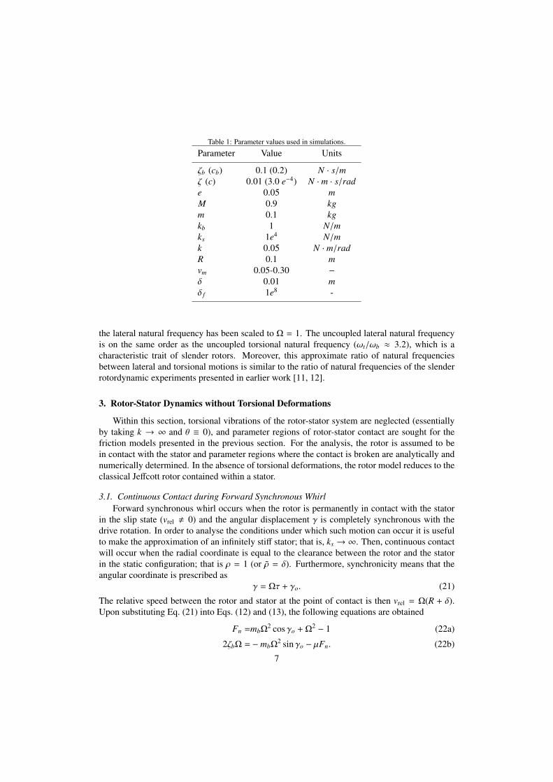
Table 1: Parameter values used in simulations.

Parameter Value Units

ζb (cb) 0.1 (0.2) N · s/mζ (c) 0.01 (3.0 e−4) N · m · s/rade 0.05 mM 0.9 kgm 0.1 kgkb 1 N/mks 1e4 N/mk 0.05 N · m/radR 0.1 mvm 0.05-0.30 −

δ 0.01 mδ f 1e8 -

the lateral natural frequency has been scaled to Ω = 1. The uncoupled lateral natural frequencyis on the same order as the uncoupled torsional natural frequency (ωt/ωb ≈ 3.2), which is acharacteristic trait of slender rotors. Moreover, this approximate ratio of natural frequenciesbetween lateral and torsional motions is similar to the ratio of natural frequencies of the slenderrotordynamic experiments presented in earlier work [11, 12].

3. Rotor-Stator Dynamics without Torsional Deformations

Within this section, torsional vibrations of the rotor-stator system are neglected (essentiallyby taking k → ∞ and θ ≡ 0), and parameter regions of rotor-stator contact are sought for thefriction models presented in the previous section. For the analysis, the rotor is assumed to bein contact with the stator and parameter regions where the contact is broken are analytically andnumerically determined. In the absence of torsional deformations, the rotor model reduces to theclassical Jeffcott rotor contained within a stator.

3.1. Continuous Contact during Forward Synchronous WhirlForward synchronous whirl occurs when the rotor is permanently in contact with the stator

in the slip state (vrel , 0) and the angular displacement γ is completely synchronous with thedrive rotation. In order to analyse the conditions under which such motion can occur it is usefulto make the approximation of an infinitely stiff stator; that is, ks → ∞. Then, continuous contactwill occur when the radial coordinate is equal to the clearance between the rotor and the statorin the static configuration; that is ρ = 1 (or ρ = δ). Furthermore, synchronicity means that theangular coordinate is prescribed as

γ = Ωτ + γo. (21)

The relative speed between the rotor and stator at the point of contact is then vrel = Ω(R + δ).Upon substituting Eq. (21) into Eqs. (12) and (13), the following equations are obtained

Fn =mbΩ2 cos γo + Ω2 − 1 (22a)

2ζbΩ = − mbΩ2 sin γo − µFn. (22b)

7

Equations (22) contain two unknowns, namely γo and Fn. It is noted that Fn is a constraint force(like a Lagrange multiplier) that arises due to the contact constraint ρ = δ. Equations (22) can becombined to solve for γo, which is given to be

γo = arcsin

−2ζbΩ + µ(Ω2 − 1)

mbΩ2√

1 + µ2

− φ, (23)

where φ is the principal value of arctan(µ). The forward whirling solution given by Eq. (21) willbe valid provided that the argument of the arcsin function is bound in magnitude by unity. Thus,the condition for forward synchronous whirl is given to be∣∣∣∣∣∣∣−2ζbΩ + µ(Ω2 − 1)

mbΩ2√

1 + µ2

∣∣∣∣∣∣∣ < 1. (24)

Equation (24) is a necessary condition for the existence of forward synchronous whirl. Note thatif this condition is true then there will be two values of γo that solve (23). As parameter valuesare varied and start to approach values for which condition (24) is violated, the two solutionscoincide. Thus the equality in (24) gives the condition for a fold bifurcation at which a stableand an unstable state of forward synchronous whirl come together and are annihilated.

Note though that Eq. (24) is not a sufficient condition for forward synchronous whirl, becausestator contact needs to be maintained. This condition is given by Fn > 0 where Fn is calculatedfrom Eq. (22a) once γo has been determined. Passage of Fn through zero would represent anon-local qualitative change in which the motion lifts off from the constraint surface ρ = δ.

It is intuitively clear that these considerations would still apply if the infinitely stiff statoris replaced with a large but finite value ks. In particular, the lift-off condition would become aboundary equilibrium bifurcation in the terminology of non-smooth system analyses [13].

In what follows, Eqs. (24) and (22a) will be used to determine regions of synchronous whirlfor the different friction models.

Figure 3 depicts regions of continuous-stator contact during forward synchronous whirl forthe different friction models. Here, the Coulomb friction model and also the cubic models forwhich µs = 1.5µm and three different values of vm are considered. The dashed vertical blackline in the figure is where the normal force Fn becomes positive, such that lift-off between rotorand stator would occur for all (µ,Ω) parameter values to the left of this curve. The shadedregions represent parameter regions of continuous forward whirling, given by the stable solutionto Eq. (23). Note that there are two solutions of µ for a fixed value of Ω in Eq. (24), whereinone value of µ is positive and the other is negative. Here, the positive value of µ is the correctroot, as the friction coefficient is assumed to be positive in the model development. Additionally,Eq. (24) yields solutions to the left of the vertical dashed line for the different friction models,which are non-physical since the normal force is of the wrong sign.

It is useful to compare the existence region for the different friction models. For lower valuesof Ω, the cubic friction model drops below the Coulomb contact line. This drop originates fromthe fact that µo > µm, and when Ω is small the effective friction is greater than µm. However,for the values of vm = 0.5, 0.25, as Ω starts to increase, the region of contact increases until theboundary comes into contact with the Coulomb friction line, upon which the boundary starts todecrease. For the case of vm = 0.1, the boundary region monotonically decreases to zero. Thismonotonic decrease occurs because the cubic friction for vm = 0.1 reaches it’s minimum valuebefore the asymptotic. For all finite values of vm, the boundary region will tend to zero in thelimit of increasing Ω since µ→ ∞ as Ω→ ∞.

8

1 2 3 4 5 6 70

0.1

0.2

0.3

0.4

0.5

0.6

0.7

0.8

0.9

1

Ω

µo

Coulomb: Whirl with ContactCubic vm = 0.50: Whirl with ContactCubic vm = 0.25: Whirl with ContactCubic vm = 0.10: Whirl with ContactFn > 0

Figure 3: Stability regions during synchronous forward whirling for Coulomb and cubic friction (µm = µo/1.5).

9

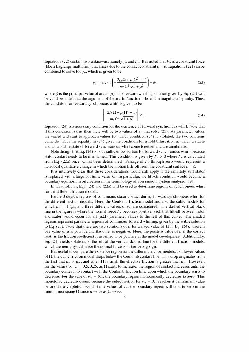
A steady-whirl with contact solution does not exist in the white-shaded region to the topright of Figure 3. Within this region, simulations indicate that their is no stable contact forwardwhirling solution (not necessary synchronous), instead the rotor always loses contact with thestator. After a significant transient period the system settles into one of two other states, ei-ther free whirling (in the direction of drive rotation) without contact or self-excited backwardwhirling. Two of the typical responses, namely, free whirling and backward whirling are pro-vided in Figure 4 for the parameter values of µ = 0.6 and Ω = 2. The trajectories of the rotorwithin the stator are shown in Figure 4(a), while the x and y time histories in Cartesian coor-dinates are shown in part (b) and the angular polar coordinate is shown in part (c). As shownin Figure 3, for this combination of µ and Ω, the rotor is also able to undergo forward whirlwith stator contact. This brings to light the point that all of these three motions (forward whirl,backward whirl, and free whirl) are dependent upon the initial conditions. In the white shadedregion to the left of the dashed line, the rotor will start free whirling or backward whirling (asshown later), depending on the initial conditions. It is noted that for the initial conditions andparameter ranges studied here, simulations did not reveal any other kinds of attractors. However,it is known that impacting motions, either periodic or chaotic, have been shown to occur in thepast by [6, 7, 14] among others. Moreover, it is noted that for the relatively large δ used in thesimulations, that the vertical dashed line (rotor-stator contact line) is relatively close to the firstlateral natural frequency. For the parameter values selected here, the rotor will only make contactwith the stator for large lateral displacements (cf. Figure 3 in [2]); however, the lateral resonanceand contact line will separate for smaller values of δ, wherein the rotor will first make contactwith the stator for small values of Ω.

3.2. Backward Whirling with Continuous Contact

Now the special case of backward whirling with continuous stator contact is addressed. Thesteady-state solution sought in this case is pure stick motion, which occurs when the relativespeed between the rotor and stator is zero. This motion is also sometimes referred to in theliterature as counter whirl, dry-friction whirl, or self-excited backward whirl.

In the current case, under the neglect of torsional deformations, the backward whirl regionwith pure stick is independent of the friction model and is only dependent upon the value of staticfriction when vrel = 0. Under the assumption that the relative speed between the rotor and statorat the point of contact is zero, representing a pure stick condition, the whirl speed of the rotorcan easily be derived from Eq. (17):

γ = −Rδ

Ω ≡ −ω

Here, the negative sign indicates that the rotor is whirling in the opposite direction to the driverotation with angular speed Ω. Bartha [8] derived conditions for backward whirling with contact,under the assumption of negligible torsional deformation, eccentricity, or mass imbalance whilethe rotor is whirling at a constant angular speed ω in contact with an infinitely stiff stator. Takingthose assumptions, force balance normally and radially at the boundary between slip and stickleads to

Mδω2 − δkb = Fn, (25a)δcbω = Fnµo. (25b)

10

−1 −0.5 0 0.5 1

−1

−0.5

0

0.5

1

x

y

(a)

0 1 2 3 4 5 6 7 8 9 10−1.5

−1

−0.5

0

0.5

1

1.5

τ

x,y

(b)

0 1 2 3 4 5 6 7 8 9 10−200

−150

−100

−50

0

50

τ

γ

(c)

Stator LocationFree WhirlBackward Whirl

Free Whirl, xFree Whirl, yBackward Whirl, xBackward Whirl, y

Free WhirlBackward Whirl

Figure 4: Typical responses for µ = 0.6, Ω = 2rad/s with Coulomb friction: (a) Rotor trajectory, (b) time histories oflateral displacement, and (c) angular polar coordinate γ.

11

Equation (25b) can then be substituted into (25a) in order to obtain the condition for the boundarybetween stick and slip; that is,

ω2stick −

2ζωn

µoωstick − ω

2n = 0, (26)

where ωn,b is the first lateral natural frequency and ζb is the corresponding damping ratio

ωn =

√kb

M, ζ =

cb

2√

kbM.

Equation (26) will yield two solutions for ωstick. One solution will not satisfy Eqs. (25), whilethe other solution gives the condition for pure stick, µ < µo or, equivalently

ω > ωstick = ωn

ζµo+

√1 +

(ζ

µo

)2 . (27)

Equation (27) can also be expressed in terms of the non-dimensional drive speed as

Ω >δ

Rωn

ωb

ζµo+

√1 +

(ζ

µo

)2 . (28)

These approximate parameter regions of rotor-stator contact during backward whirl are plot-ted in Figure 5.

Note that in this approximate formulation, Fn is assumed to be constant during the motion.In practice, when non-vanishing eccentricity and mass imbalance are taken into account, thenormal force will undergo oscillation about this nominal value due to the nonautonomous termsin equations (12), (13), and (14). Specifically, the normal force in equations (22a) will have atemporal dependence.

It should be noted that the regions shown in Figure 5 are strictly only relevant for findingregions of backward whirl (pure stick). In the red-shaded region, the rotor may in fact undergoforward synchronous whirling with or without stator contact. Rather than consider the effectsof imbalance and eccentricity separately on these existence regions, we shall in the next sectionconsider these effects in combination with torsional deformation.

4. Rotor-Stator Dynamics with Torsional Deformations

We now consider the effect of torsional deformation on the stability boundaries computed inthe previous section. As before, forward whirling will be considered first, following by the caseof backward whirling.

4.1. Forward Whirl with Torsional Deformations

Similar to case without torsional deformations we seek steady whirl solutions of the form

θ = θo and (29a)γ = Ωτ + γo. (29b)

12

0 0.5 1 1.5 2 2.5 30

0.05

0.1

0.15

0.2

0.25

Ω

µo

No Backward Whirl SolutionBackward Whirl without SlipFn > 0

Figure 5: Approximate regions of pure stick and slip with rotor-stator contact under the assumption of negligible torsionaldeformations, mass imbalance, and eccentricity, given by solutions to Eq. (27).

Equations (29) can be substituted into Eqs. (12) and (13), while allowing ρ = 1. This leads tononlinear equations that have to be solved for the unknown constants γo and θo:

θo − γo = arcsin

−2ζbΩ + µ(Ω2 − 1)

mbΩ2√

1 + µ2

− φ, (30a)

ω2t

ω2b

θo = −mtΩ2 sin(θo − γo) − m fµ

[mbΩ2 cosψ + Ω2 − 1

], (30b)

where φ is again the principal value of arctan(µ). In order to determine the stability of thissolution, it is helpful to write

γ(τ) = γ(τ) + Ωτ + γo and (31a)

θ(τ) = θ(τ) + θo, (31b)

where the quantities with a carrot on top are assumed to be small perturbations to the steadywhirl solution determined by Eqs. (30). Equations (31) can be substituted into Eqs. (12)-(14),and written in vector notation as

x′ = FFW(x), (32)

13

where xT = γ, θ, ˙γ, ˙θ and the superscript T denotes the vector transpose operation. An explicitexpression for FFW takes the form:

FFW =

˙γ,˙θ,[

1 mb(µ sinψ + cosψ)−mt cosψ 1 + µmbm f sinψ

]−1 −2ζt(γ′ + Ω) + mb(Ω + θ′) sinψ − µF−2ζtθ

′ −ω2

t

ω2b(θo + θ) − mt(γ′ + Ω)2 sinψ − m fµF

,(33)

where

ψ =γo − γ + θo + θ (34)

F =mb(Ω + θ′)2 cosψ + (γ′ + Ω)2 − 1 (35)

The parameter regions in which steady forward-whirl solutions occur (γo, θo) occur, for twodifferent values of torsional damping ζt is plotted in Figure 6. Note the similarity of these exis-tence regions to those shown in Figure 3. Furthermore, for each equilibrium, the eigenvalues ofFFW have been computed and give the conditions for instability. The yellow and green regionsin Figure 6 depict parameter regions in which the equilibrium is unstable with complex conju-gate eigenvalues. The boundary of this region represents a Hopf bifurcation. The yellow regionsdepicts where, during the ensuing torsional oscillations, the rotor looses contact with the stator(determined by Fn < 0). The green regions depict where the rotor stays in contact and undergoeslimit cycle oscillations. As can be seen from Figure 6, increasing the torsional damping reducesthe region where the rotor breaks contact with the stator.

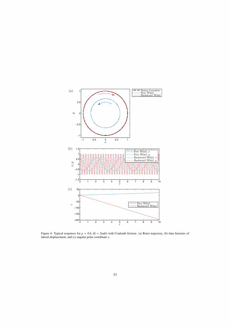
One-parameter bifurcation diagrams corresponding to variation of Ω for fixed values of µo

for the two cases shown in Figure 6(a) and (b) are shown in Figure 7(a) and (b). The results arecomputed numerically by direct integration; hence, only the stable motion branch is depicted.The results are shown in a Poincare section corresponding to maxima of γ. Figure 7(a), which isthe case of no torsional damping is indicative of a supercritical Hopf bifurcation upon reductionof Ω. Additionally, inspection of the numerically computed eigenvalues, although not provided,indicate a Hopf bifurcation point. The limit cycle grows in amplitude upon further reduction of Ω

until a point is reached for which Fn < 0 and the motion lifts off. A supercritical Hopf bifurcationis also observed in the case shown in Figure 7(b) for which ζt = 0.01. As Ω is increased beyondthe bifurcation point, a period-doubling bifurcation is observed before the rotor breaks contactwith the stator.

Figure 8 presents similar results for the cubic friction model, taking specifically the caseζt = 0.1 and vm = 1. Looking at a one-parameter slice through the oval shaped region withµo ≈ 0.1 reveals another supercritical Hopf bifurcation, followed by a period doubling bifurcationbefore loss of contact ensues (results not shown). However, in the upper-left hand portion ofFigure 8, there exists another region where torsional oscillations are present with rotor-statorcontact. Here, the system still experiences a Hopf instability, but the amplitude of the oscillationsare small.

4.2. Self-Excited Backward Whirling

Here, an exact contact condition will be sought including the combined effects of mass im-balance, eccentricity, and torsional deformation. As noted earlier, during backward self-exited

14

1 2 3 4 5 6 70

0.2

0.4

0.6

0.8

1

Ω

µo

(a) ζt = 0.00

No Torsional Motions with ContactTorsional Motions with ContactLoss of ContactFn > 0

1 2 3 4 5 6 70

0.2

0.4

0.6

0.8

1

Ω

µo

(b) ζt = 0.01

Figure 6: Parameter regions of existence and stability of synchronous forward whirling with torsional deformation in thecase of Coulomb friction with (a) ζt = 0 and (b) ζt = 0.01.

15

2.5 2.55 2.6 2.65 2.70

0.05

0.1

0.15

0.2

0.25

0.3

0.35

Ω

γ

(a) ζt = 0, µ = 0.35

3 3.05 3.1 3.15 3.2 3.25 3.3 3.35 3.40

0.1

0.2

0.3

0.4

0.5

0.6

0.7

0.8

0.9

Ω

γ

(b) ζt = 0.01, µ = 0.10

Figure 7: Bifurcation diagrams from sections taken from Figure 6 for (a) ζt = 0, µo = 0.35 and (b) ζt = 0.01, µo = 0.10.

16

1 2 3 4 5 6 70

0.1

0.2

0.3

0.4

0.5

0.6

0.7

0.8

0.9

1

Ω

µo

No Torsional Motions with ContactTorsional Motions with ContactLoss of ContactFn > 0

Figure 8: Regions of stability for cubic friction with parameters ζt = 0.01, vm = 1, and µm = µo/1.5.

whirl γ′ ≈ −RδΩ. However, an equation of the form

γ = −Rδ

Ωτ + γo, (36)

where γo is a constant, can never satisfy Eq. (13) because of the mass imbalance and eccentricityterms. In order to search for non-equilibrium backward whirling solutions in this case, againthe analysis considers the rigid limit by constraining the radial displacement such that ρ = 1.Perturbed quantities in γ and θ are sought of the form

γ = −Rδ

Ωτ + γ and (37)

θ =θ, (38)

Upon substituting these relations into Eqs. (12), (13), and (14), the normal force Fn becomes aconstraint force (like a Lagrange multiplier) which can be directly calculated from Eq. (12). Theremaining two equations can be put into vector notation and may be compactly written as

x′ = FBW(x, τ). (39)

The equations (39) are then solved numerically to look for steady-state solutions for whichthe normal force remains positive. In numerically solving Eq. (39), Coulomb friction is appliedunder the approximation (20) with δ f set to 1 × 108, and the relative tolerance of the Runge-Kutta numerical integrator was set to 1 × 10−8. Studies were conducted by varying both of thesequantities, and the chosen values were found to give sufficiently accurate results.

A summary of the results is given in Figure 9. For illustrative purposes, the line defining theboundary of backward whirling solution without torsional deformations and eccentricity, given

17

0.5 1 1.5 2 2.5 3

0.03

0.04

0.05

0.06

0.07

0.08

0.09

0.1

Ω

µo

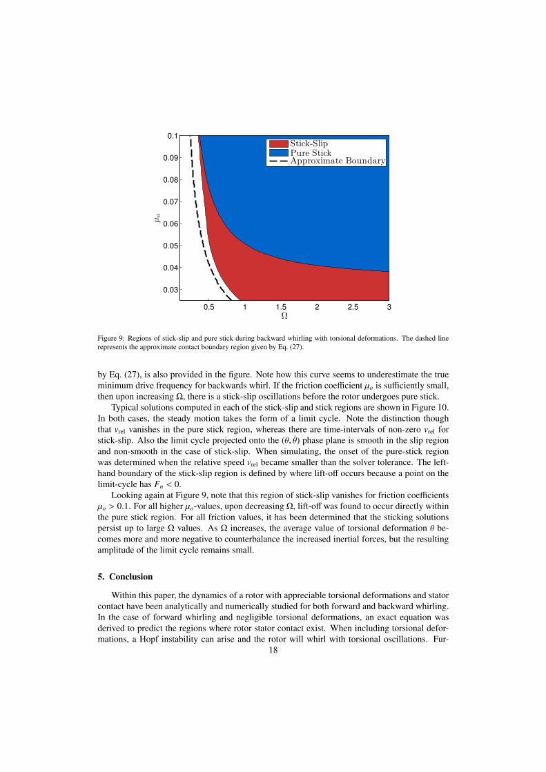
Stick-SlipPure StickApproximate Boundary

Figure 9: Regions of stick-slip and pure stick during backward whirling with torsional deformations. The dashed linerepresents the approximate contact boundary region given by Eq. (27).

by Eq. (27), is also provided in the figure. Note how this curve seems to underestimate the trueminimum drive frequency for backwards whirl. If the friction coefficient µo is sufficiently small,then upon increasing Ω, there is a stick-slip oscillations before the rotor undergoes pure stick.

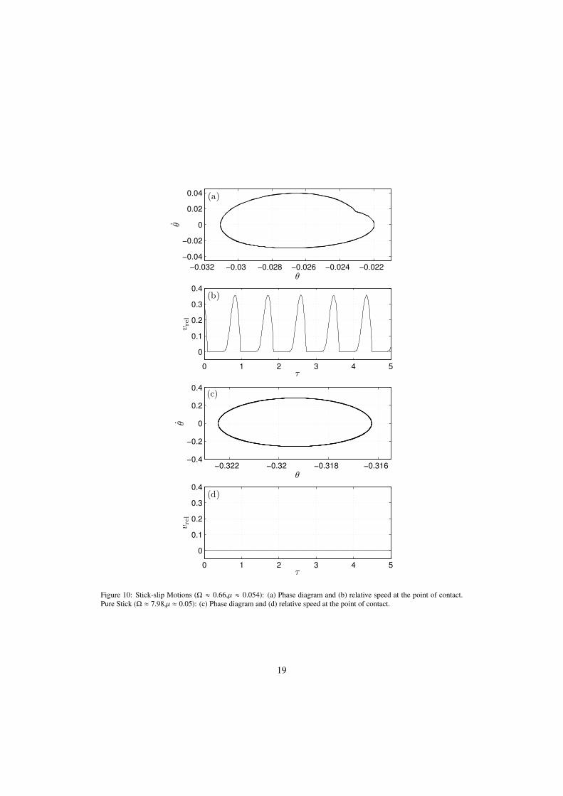
Typical solutions computed in each of the stick-slip and stick regions are shown in Figure 10.In both cases, the steady motion takes the form of a limit cycle. Note the distinction thoughthat vrel vanishes in the pure stick region, whereas there are time-intervals of non-zero vrel forstick-slip. Also the limit cycle projected onto the (θ, θ) phase plane is smooth in the slip regionand non-smooth in the case of stick-slip. When simulating, the onset of the pure-stick regionwas determined when the relative speed vrel became smaller than the solver tolerance. The left-hand boundary of the stick-slip region is defined by where lift-off occurs because a point on thelimit-cycle has Fn < 0.

Looking again at Figure 9, note that this region of stick-slip vanishes for friction coefficientsµo > 0.1. For all higher µo-values, upon decreasing Ω, lift-off was found to occur directly withinthe pure stick region. For all friction values, it has been determined that the sticking solutionspersist up to large Ω values. As Ω increases, the average value of torsional deformation θ be-comes more and more negative to counterbalance the increased inertial forces, but the resultingamplitude of the limit cycle remains small.

5. Conclusion

Within this paper, the dynamics of a rotor with appreciable torsional deformations and statorcontact have been analytically and numerically studied for both forward and backward whirling.In the case of forward whirling and negligible torsional deformations, an exact equation wasderived to predict the regions where rotor stator contact exist. When including torsional defor-mations, a Hopf instability can arise and the rotor will whirl with torsional oscillations. Fur-

18

−0.032 −0.03 −0.028 −0.026 −0.024 −0.022

−0.04

−0.02

0

0.02

0.04

θ

θ

(a)

0 1 2 3 4 5

0

0.1

0.2

0.3

0.4

τ

v rel

(b)

−0.322 −0.32 −0.318 −0.316−0.4

−0.2

0

0.2

0.4

θ

θ

(c)

0 1 2 3 4 5

0

0.1

0.2

0.3

0.4

τ

v rel

(d)

Figure 10: Stick-slip Motions (Ω ≈ 0.66,µ ≈ 0.054): (a) Phase diagram and (b) relative speed at the point of contact.Pure Stick (Ω ≈ 7.98,µ ≈ 0.05): (c) Phase diagram and (d) relative speed at the point of contact.

19

thermore, in certain regions the rotor response can exhibit a period doubling bifurcation. A keydevelopment here is to show that these oscillations can occur independently of the chosen frictionmodel. This expands the analysis in [2] where the mechanism for Hopf bifurcation was found tobe due to the negative slope in the cubic model. Note that the additional small amplitude limitcycles found in the upper left-hand portion of Figure 8 may well be related to those analyzed inthe previous work [2].

In the second case of backward whirl with stator contact, we found evidence for transitionbetween two types of motion, namely, stick-slip and pure stick motions. During stick-slip, therelative speed between the rotor and stator reaches zero for a finite amount of time, then slips freewith positive relative speed. We have also shed light on the nature of the self-excited backwardwhirl, that it should represent periodic motion, rather than a radial equilibrium and that oscillationin both the torsional degree of freedom and relative angular position of the contact point mustoccur.

The findings within this work have applications to rotor systems with stator contact and largetorsional deformations. Generally speaking, forward whirl, which represents pure slip motionoccurs for smaller values of the friction coefficient, whereas backward whirl is likely to occur forsufficiently large friction. Note though, we find significant parameter regimes where both forwardand backward whirl can coexist. Nevertheless, backward whirl appears somewhat more robust.Specifically, within the forward whirling regime, inclusion of a torsional degree of freedom cancause oscillations that quickly grow in amplitude so as to destroy the continuous contact. Also,small change in the details of the friction model or of torsional damping can cause significantdifferences to the existence and stability region of forward whirl. In contrast, we have found noevidence of instabilities during backward whirl other than at its small-Ω limit of existence. Wealso note how the analytic approximation (27) provides the correct trend for this lower rotationspeed for backward whirl; however, this trend is a conservative estimate.

Acknowledgement

This work was supported by the EPSRC Programme Grant “Engineering Nonlinearity” EP/K003836/2.This work was partially supported by U.S. NSF Grant No. CMMI1436141.

References

[1] H. Jeffcott, The lateral vibrations of loaded shafts in the neighbourhood of a whirling speed - the effect of want ofbalance, Philosophical Magazine 37 (1919) 304–314.

[2] N. Vlajic, X. Liu, H. Karki, B. Balachandran, Torsional oscillations of a rotor with continuous stator contact,International Journal of Mechanical Sciences 83 (2014) 65–75.

[3] S. Edwards, A. Lees, M. Friswell, The influence of torsion on rotor/stator contact in rotating machinery, Journalof Sound and Vibration 225 (1999) 767–778.

[4] N. Mihajlovic, A. van Veggel, N. van de Wouw, H. Nijmeijer, Analysis of friction-induced limit cycling in anexperimental drill-string system, ASME Journal of Dynamic Systems, Measurement, and Control 126 (2004)709–720.

[5] N. Mihajlovic, N. van de Wouw, P. Rossielle, H. Nijmeijer, Interaction between torsional and lateral vibrations inflexible rotor systems with discontinuous friction, Nonlinear Dynamics 50 (2007) 679–699.

[6] F. Chu, Z. Zhang, Bifurcation and chaos in a rub-impact jeffcott rotor system, Journal of Sound and Vibration 210(1998) 1–18.

[7] Z. Feng, X. Zhang, Rubbing phenomena in rotor-stator contact, Chaos, Solitons & Fractals 14 (2002) 257–267.[8] A. Bartha, Dry Friction Backward Whirl of Rotors, PhD Thesis, Swiss Federal Institute of Technology, Zurich,

Switzerland, 2000.

20

[9] D. Childs, A. Bhattacharya, Prediction of dry-friction whirl and whip between a rotor and a stator, Journal ofVibration and Acoustics 129 (2007) 355–362.

[10] X. Liu, N. Vlajic, X. Long, G. Meng, B. Balachandran, Nonlinear motions of a flexible rotor with a drill bit:stick-slip and delay effects, Nonlinear Dynamics 72 (2013) 61–77.

[11] N. Vlajic, X. Liu, H. Karki, B. Balachandran, Rotor torsion vibrations in the presence of continuous stator contact,ASME IMECE, DETC2012/MECH-89195 (2012).

[12] N. Vlajic, C.-M. Liao, H. Karki, B. Balachandran, Stick-slip motions of a rotor-stator system, Journal of Vibrationand Acoustics 136 (2014) 021005.

[13] M. Bernardo, C. Budd, A. R. Champneys, P. Kowalczyk, Piecewise-smooth dynamical systems: theory and appli-cations, volume 163, Springer Science & Business Media, 2008.

[14] E. V. Karpenko, M. Wiercigroch, M. P. Cartmell, Regular and chaotic dynamics of a discontinuously nonlinearrotor system, Chaos, Solitons & Fractals 13 (2002) 1231–1242.

21