Embed Size (px)
Citation preview
i
Features of the Hilbert Book Model.
The HBM is a simple Higgsless model of fundamental
physics that is strictly based on the axioms of traditional
quantum logic. It uses a sequence of instances of an exten-
sion of a quaternionic separable Hilbert space that each
represents a static status quo of the whole universe.
Features of the
Hilbert Book Model
Hans van Leunen
The Hilbert Book Model
ii
FEATURES OF THE HILBERT BOOK MODEL
iii
Colophon
Written by Ir J.A.J. van Leunen
The subject of this book is a new model of physics
This book is written as an e-book. It contains hyperlinks that become active in the electronic
version. That version can be accessed at http://www.crypts-of-physics.eu. Last update of this
(published) version: Tuesday, May 01, 2012
This book is currently in preparation phase so it may change regularly.
©2012 Ir J.A.J. (Hans) van Leunen
All rights reserved. Nothing of these articles may be copied or translated without the written
permission of the publisher, except for brief excerpts for reviews and scientific studies that refer
to this resource.
ISBN: t.b.d.978-1-4477-1684-6
iv
Ir J.A.J. van Leunen
FEATURES OF THE HILBERT BOOK MODEL
v
ACKNOWLEDGEMENTS
I thank my wife Albertine, who tolerated me to work days and nights on a subject that can only
be fully comprehended by experts in this field. For several years she had to share me with my text
processor. She stimulated me to bring this project to a feasible temporary end, because this project
is in fact a never ending story.
I also have to thank my friends and discussion partners that listened to my lengthy delibera-
tions on this non society chitchat suitable subject and patiently tolerated that my insights changed
regularly.
vi
DETAILS
The Hilbert Book Model is the result of a still ongoing research project.
That project started in 2009.
The continuing status of the project can be followed at
http://www.crypts-of-physics.eu
The author’s e-print site is:
http://vixra.org/author/j_a_j_van_leunen.
This book is accompanied by a slide show at
http://vixra.org/abs/1202.0033
The nice thing about laws of physics is that they repeat themselves. Otherwise they would not
be noticed. The task of physicists is to notice the repetition.

vii
viii
Contents
PART I ................................................................................................................. 17
The fundaments ................................................................................................... 17
1 FUNDAMENTS ........................................................................................ 19 1.1 Logic model ......................................................................................... 19 1.2 State functions ..................................................................................... 20 1.3 The sandwich ....................................................................................... 21 1.4 Model dynamics .................................................................................. 22 1.5 Quaternionic versus complex Hilbert space ........................................ 24 1.6 Advantages of QPAD’s ....................................................................... 25 1.7 Sign flavors .......................................................................................... 26 1.8 Virtual carriers and interactions ........................................................... 26 1.9 QPAD-sphere ...................................................................................... 27 1.10 The HBM Palestra ............................................................................... 30 1.11 Dynamics control ................................................................................. 30
1.11.1 Quantum mechanics .................................................................... 31 1.11.2 Quantum fluid dynamics ............................................................. 31 1.11.3 Elementary coupling ................................................................... 31
1.12 Fields ................................................................................................... 32
2 History ....................................................................................................... 33 2.1 Criticism .............................................................................................. 34
2.1.1 Model .......................................................................................... 34 2.1.2 Quaternions ................................................................................. 34 2.1.3 Quaternionic versus complex probability amplitude distributions35
2.2 Consequence ........................................................................................ 35
PART II ............................................................................................................... 36
The Hilbert Book Model ..................................................................................... 36
3 INGREDIENTS ........................................................................................ 37 3.1 Role of the particle locator operator .................................................... 37 3.2 QPAD’s ............................................................................................... 37 3.3 Helmholtz decomposition .................................................................... 38 3.4 QPAD vizualization ............................................................................. 38 3.5 QPAD categories ................................................................................. 39 3.6 Special composed QPAD’s ................................................................. 39
3.6.1 The average QPAD ..................................................................... 40 3.7 The background QPAD ....................................................................... 40
ix
3.7.2 Isotropy ....................................................................................... 41 3.8 Physical fields ...................................................................................... 41 3.9 Inertia ................................................................................................... 41 3.10 Coupling and curvature ....................................................................... 42 3.11 Hyper-complex numbers ..................................................................... 44 3.12 Quaternions.......................................................................................... 44
3.12.1 Sign selections ............................................................................ 44 3.12.2 Habits .......................................................................................... 46
3.13 Quaternionic distributions ................................................................... 46 3.13.1 Sign flavors ................................................................................. 47 3.13.2 QD multiplication ....................................................................... 47 3.13.3 Differentiation and Fourier transform ......................................... 47 3.13.4 Spinors and matrices ................................................................... 48 3.13.5 Continuity equation ..................................................................... 50
3.14 Hilbert space ........................................................................................ 51
4 PARTICLE PHYSICS.............................................................................. 54 4.1 Elementary coupling equation ............................................................. 54 4.2 Restricted elementary coupling ........................................................... 54
4.2.1 Dirac equation ............................................................................. 55 4.2.2 The Majorana equation ............................................................... 57 4.2.3 The next particle type ................................................................. 58
4.3 Massles bosons .................................................................................... 59 4.3.1 No coupling ................................................................................ 59 4.3.2 The free QPAD ........................................................................... 60
4.4 Consideration ....................................................................................... 61 4.5 Anisotropic coupling fields ................................................................. 62
4.5.1 The cross-sign flavor equations .................................................. 62 4.5.2 The Z boson ................................................................................ 63
4.6 Resulting particles ............................................................................... 64 4.7 Antiparticles ........................................................................................ 64 4.8 Shadow particles .................................................................................. 64 4.9 Table of elementary particles............................................................... 65 4.10 Limits of the model ............................................................................. 66
5 Origin of curvature ................................................................................... 68 5.1 Physical fields ...................................................................................... 68 5.2 Curvature and inertia ........................................................................... 68
5.2.1 Inertia versus antiparticle ............................................................ 68 5.2.2 Inertia of W and Z Bosons .......................................................... 69
5.3 Effect of primary coupling .................................................................. 69 5.4 The HBM Palestra reviewed ................................................................ 70 5.5 What image intensifiers reveal ............................................................ 71 5.6 Quantum Fluid Dynamics .................................................................... 72
6 Higher level coupling ................................................................................ 73
x
6.1 A quaternionic theory of general relativity .......................................... 73 6.2 The Kerr-Newman equation ................................................................ 73 6.3 Role of second category physical fields .............................................. 73 6.4 Higgs ................................................................................................... 73
7 HADRONS ................................................................................................ 75 7.1 Second level coupling .......................................................................... 75 7.2 Interaction ............................................................................................ 76 7.3 Rules .................................................................................................... 76 7.4 Up-quarks ............................................................................................ 77 7.5 Mesons ................................................................................................. 77 7.6 Baryons ................................................................................................ 77
8 THE BUILDING ....................................................................................... 78 8.1 Natures Music ...................................................................................... 78 8.2 Hydrogen atom .................................................................................... 78 8.3 Helium atom ........................................................................................ 78 8.4 Modularization .................................................................................... 78 8.5 Black hole ............................................................................................ 79
8.5.1 Classical black hole .................................................................... 79 8.5.2 Simple black hole........................................................................ 80 8.5.3 General black hole ...................................................................... 80 8.5.4 Quantum black hole .................................................................... 80 8.5.5 Holographic principle ................................................................. 81 8.5.6 Black hole as a subspace of the Hilbert space ............................. 81 8.5.7 HBM interpretation of black hole ............................................... 82 8.5.8 Chandrasekhar limit .................................................................... 82 8.5.9 Similarity between black hole and massive fermion ................... 83
8.6 Birth of the universe ............................................................................ 83
9 COSMOLOGY .......................................................................................... 87 9.1 Higher order couplings ........................................................................ 87 9.2 Curvature ............................................................................................. 88
9.2.1 Hilbert Book Model ingredients ................................................. 88 9.2.2 Coordinate system....................................................................... 89 9.2.3 Metric .......................................................................................... 89 9.2.4 Scales .......................................................................................... 90
9.3 Inside black holes ................................................................................ 92 9.4 Hadrons ............................................................................................... 92
10 CONCLUSION ......................................................................................... 93
PART III .............................................................................................................. 94
Appendix .............................................................................................................. 94
xi
1 Logic ........................................................................................................... 95 1.1 History of quantum logic ..................................................................... 95 1.2 Quantum logic ..................................................................................... 95
1.2.1 Lattices ........................................................................................ 95 1.2.2 Proposition .................................................................................. 98 1.2.3 Observation ................................................................................. 99
2 Numbers ..................................................................................................... 99 2.1 Cayley-Dickson onstruction ................................................................ 99 2.2 Warren Smith’s numbers ................................................................... 100
2.2.1 2n-on construction ..................................................................... 100
2.3 Quaternions........................................................................................ 102 2.3.1 Sign selections .......................................................................... 102 2.3.2 Colored signs ............................................................................ 106 2.3.3 Waltz details ............................................................................. 106
2.4 Quaternion coordinates ...................................................................... 109 2.4.1 Polar coordinates....................................................................... 109 2.4.2 3 sphere ..................................................................................... 110 2.4.3 Hopf coordinates ....................................................................... 111 2.4.4 Group structure ......................................................................... 111 2.4.5 Versor ....................................................................................... 112 2.4.6 Symplectic decomposition ........................................................ 112
3 Quaternionic distributions ..................................................................... 113 3.1 Sign flavors ........................................................................................ 113 3.2 Differentiation ................................................................................... 113 3.3 Fourier transform ............................................................................... 113 3.4 Helmholtz decomposition .................................................................. 114
4 Fields ........................................................................................................ 115 4.1 The origin of physical fields. ............................................................. 115
4.1.1 Categories of fields ................................................................... 115 4.2 Example potential .............................................................................. 116
5 Fourier transform ................................................................................... 118 5.1 Quaternionic Fourier transform split ................................................. 118 5.2 Alternative transverse plane .............................................................. 120 5.3 Alternative approach to Fourier transform ........................................ 120 5.4 Weil-Brezin transform ....................................................................... 121 5.5 Fourier transform ............................................................................... 122 5.6 Functions invariant under Fourier transform ..................................... 122 5.7 Special Fourier transform pairs ......................................................... 127 5.8 Complex Fourier transform invariance properties ............................. 127 5.9 Fourier transform properties .............................................................. 127
5.9.1 Parseval’s theorem .................................................................... 127 5.9.2 Convolution .............................................................................. 128
xii
5.9.3 Differentiation ........................................................................... 128
6 Ladder operator ...................................................................................... 128
7 States ........................................................................................................ 130 7.1 Ground state....................................................................................... 130 7.2 Coherent state .................................................................................... 131 7.3 Squeezing .......................................................................................... 133
8 Base transforms ....................................................................................... 133
9 Oscillations .............................................................................................. 134 9.1 Harmonic oscillating Hilbert field ..................................................... 134 9.2 Annihilator and creator ...................................................................... 135 9.3 Rotational symmetry.......................................................................... 136 9.4 Spherical harmonics .......................................................................... 136 9.5 Spherical harmonic transform............................................................ 139 9.6 Polar coordinates ............................................................................... 140 9.7 Spherical coordinates ......................................................................... 140 9.8 The spherical harmonic transform ..................................................... 141 9.9 The Fourier transform of a black hole ............................................... 142 9.10 Spherical harmonics eigenvalues ....................................................... 142 9.11 Orbital angular momentum ................................................................ 144 9.12 Spherical harmonics expansion ......................................................... 146 9.13 Spin weighted spherical harmonics ................................................... 146 9.14 Eth ..................................................................................................... 148 9.15 Spin-weighted harmonic functions .................................................... 148
10 Differentiation ......................................................................................... 149 10.1 Continuity equation ........................................................................... 150
10.1.1 Continuity Equations ................................................................ 151 10.2 Discrete distribution .......................................................................... 153 10.3 Differential potential equations ......................................................... 153
10.3.1 In Fourier space ........................................................................ 154 10.4 Maxwell equations ............................................................................. 155
10.4.1 Differentiable distribution ......................................................... 156
11 Conservation laws ................................................................................... 156 11.1 Flux vector ......................................................................................... 156 11.2 Conservation of energy ...................................................................... 156 11.3 How to interprete Umechanical .................................................................. 157 11.4 Conservation of linear momentum .................................................... 158 11.5 Conservation of angular momentum ................................................. 159
11.5.1 Field angular momentum .......................................................... 159 11.5.2 Spin ........................................................................................... 160 11.5.3 Spin discussion ......................................................................... 161
xiii
12 The universe of items .............................................................................. 163 12.1 Inertia ................................................................................................. 163 12.2 Nearby items ...................................................................................... 166 12.3 Rotational inertia ............................................................................... 166 12.4 Computation of the background QPAD............................................. 167
13 Path characteristics ................................................................................. 168 13.1 Path equations .................................................................................... 169 13.2 Curve length ...................................................................................... 169 13.3 Reparameterization ............................................................................ 169
14 Metric tensor field ................................................................................... 170 14.1 Curved path ....................................................................................... 170 14.2 Calculus of variations ........................................................................ 171 14.3 Affine geometry ................................................................................. 171 14.4 Christoffel symbols ........................................................................... 172 14.5 Local metric equation ........................................................................ 173
14.5.1 Kerr-Newman metric equation ................................................. 174 14.5.2 Schwarzschild metric ................................................................ 178
15 The action along the live path ................................................................ 181 15.1 Noether’s theorem ............................................................................. 182
16 Quaternionic metric ................................................................................ 183
17 References ................................................................................................ 183
INDEX ................................................................................................................ 187
14
Preface
I started the Hilbert Book Model during my studies in physics in the sixties on the Technical
University of Eindhoven (TUE).
In the first two years the lectures concerned only classical physics. In the third year quantum
physics was introduced. I had great difficulty in understanding why the methodology of doing
physics changed drastically. So I went to the teacher, which was an old nearly retired professor
and asked him:
"Why is quantum mechanics done so differently from classical mechanics?".
His answer was short. He stated":
"The reason is that quantum mechanics is based on the superposition principle".
I quickly realized that this was part of the methodology and could not be the reason of the dif-
ference in methodology. So I went back and told him my concern. He told me that he could not
give me a better answer and if I wanted a useful answer I should research that myself. So, I first
went to the library, but the university was quite new and its library only contained rather old se-
cond hand books, which they got from other institutions. Next I went to the city’s book shops. I
finally found a booklet from P. Mittelstaedt: (Philosophische Probleme der modernen Physik, BI
Hochschultaschenbücher, Band 50, 1963) that contained a chapter on quantum logic. Small parti-
cles obey a kind of logic that differs from classical logic. As a result their dynamic behavior dif-
fers from the behavior of larger objects. I concluded that this produced the answer that I was look-
ing for.
I searched further and encountered papers from Garret Birkhoff and John von Neumann that
explained the correspondence between quantum logic and separable Hilbert spaces. That produced
a more conclusive answer to my question.
The lectures also told me that observables were related to eigenvalues of Hermitian operators.
These eigenvalues are real numbers. However, it was clearly visible that nature has a 3+1D struc-
ture. So I tried to solve that discrepancy as well. After a few days of puzzling I discovered a num-
ber system that had this 3+1D structure and I called them compound numbers. I went back to my
professor and asked him why such compound numbers were not used in physics. Again he could
not give a reasonable answer.
When I asked the same question to a much younger assistant professor he told me that these
numbers were discovered more than a century earlier by William Rowan Hamilton when he was
walking with his wife over a bridge in Dublin. He was so glad about his discovery that he carved
the formula that treats the multiplication of these numbers into the sidewall of the bridge. The in-
scription has faded away, but it is now molded in bronze and fixed to the same wall. The numbers
are known as quaternions. So, I went to the library and searched for papers on quaternions.
In those years C. Piron wrote his papers on quaternionic Hilbert spaces. That information com-
pleted my insight in this subject. I finalized my physics study with an internal paper on quaterni-
onic Hilbert spaces.
The university was specialized in applied physics and not in theoretical physics. This did not
stimulate me to proceed with the subject. Next, I went into a career in industry where I used my
knowledge of physics in helping to analyze intensified imaging and in assisting with the design of
night vision equipment and X-ray image intensifiers. That put me with my nose on the notion of
quanta.
15
The output window of image intensifiers did not show radiation. Instead they showed clouds of
impinging quanta. In those times I had not much opportunity to deliberate on that fact. However,
after my retirement I started to rethink the matter. That was the instant that the Hilbert Book
Model continued further.
Thus, in a few words: The Hilbert Book Model tries to explain the existence of quanta. It does
that by starting from traditional quantum logic.
The Hilbert Book Model is a Higgsless model of physics. It explains how elementary particles
get their mass.
You will find the model to be in many aspects controversial and non-conventional. That is why
the author took great efforts in order to keep the model self-consistent.

16
If a mathematical theory is self-consistent, then there is a realistic chance that nature some-
where somehow uses it.
If that theory is compatible with traditional quantum logic, then there is a large chance that
nature will use it.
This drives my intuition.
HvL
17
PART I The fundaments
Abstract
The fundaments of quantum physics are still not well established. This book tries to find the
cracks in these fundaments and explores options that were left open. This leads to unconventional
solutions and a new model of physics.
In order to optimize self-consistency, the model is strictly based on the axioms of traditional
quantum logic. Traditional quantum logic is lattice isomorphic to the set of closed subspaces of an
infinite dimensional separable Hilbert space. It means that the separable Hilbert space can be used
as the realm in which quantum physics will be modeled. However, this would result in a rather
primitive model. It can easily be shown that this model cannot implement dynamics and does not
provide fields.
First, the model is extended such that it can represent fields. This results in a model that can
represent a static status quo of the whole universe. The most revolutionary introduction in the
Hilbert Book Model is the representation of dynamics by a sequence of such static models in the
form of a sequence of extended separable Hilbert spaces.
At this point the Hilbert Book Model already differs significantly from conventional physics.
Conventional quantum physics does not strictly hold to the axioms of traditional quantum logic,
handles fields in a different way and implements dynamics differently.
Conventional quantum physic stays with complex state functions1. In contrast the HBM also
explores the full potential of quaternionic state functions. As a consequence the HBM offers two
1 The HBM uses the name state function for the quantum state of an object or system rather than the usual
term wave function because the state function may characterize flow behavior as well as wave behavior.
18
different views on the undercrofts of quantum physics. The complex state function offers a wave
dynamics view. The quaternionic state function opens a fluid dynamics view.
The quaternionic state functions enable the exploration of the geometry of elementary particles
in which quaternionic sign flavors play an important role.
In the HBM elementary particles and physical fields are generated via the coupling of two sign
flavors of the same quaternionic probability amplitude distribution (QPAD).
The quantum fluid dynamic view opens insight in the effect of the state functions on space
curvature.
19
1 FUNDAMENTS
The most basic fundaments consist of quantum logic, its lattice isomorphic companion, the
separable Hilbert space and the extensions of these basic models such that they incorporate fields.
1.1 Logic model
In order to safeguard a high degree of consistency, the author has decided to base the Hilbert
Book Model on a consistent set of axioms. It is often disputed whether a model of physics can be
strictly based on a set of axioms. Still, what can be smarter than founding a model of physics on
the axioms of classical logic?
Since in 1936 John von Neumann2 wrote his introductory paper on quantum logic the scientific
community knows that nature cheats with classical logic. Garret Birkhoff and John von Neumann
showed that nature is not complying with the laws of classical logic. Instead nature uses a logic in
which exactly one of the laws is weakened when it is compared to classical logic. As in all situa-
tions where rules are weakened, this leads to a kind of anarchy. In those areas where the behavior
of nature differs from classical logic, its composition is a lot more complicated. That area is the
site of the very small items. Actually, that area is in its principles a lot more fascinating than the
cosmos. The cosmos conforms, as far as we know, nicely to classical logic. In scientific circles
the weakened logic that is discussed here is named traditional quantum logic.
As a consequence the Hilbert Book Model will be strictly based on the axioms of traditional
quantum logic. However, this choice immediately reveals its constraints. Traditional quantum log-
ic is not a nice playground for the mathematics that characterizes the formulation of most physical
laws. Lucky enough, von Neumann encountered the same problem and together with Garret
Birkhoff3 he detected that the set of propositions of quantum logic is lattice isomorphic with the
set of closed subspaces of an infinite dimensional separable Hilbert space. The realm of a Hilbert
space is far more suitable for performing the mathematics of quantum physics than the domain of
traditional quantum logic. Some decades later Constantin Piron4 proved that the inner product of
the Hilbert space must by defined by numbers that are taken from a division ring. Suitable divi-
sion rings are the real numbers, the complex numbers and the quaternions5. The Hilbert Book
Model also considers the choice with the widest possibilities. It uses both complex and quaterni-
onic Hilbert spaces. However, quaternions play a decisive role in the design of the Hilbert Book
Model. Higher dimension hyper-complex numbers may suit as eigenvalues of operators or as val-
ues of physical fields, but for the moment the HBM can do without these numbers. Instead, at the
utmost quaternions will be used for those purposes.
2http://en.wikipedia.org/wiki/John_von_Neumann#Quantum_logics 3 http://en.wikipedia.org/wiki/John_von_Neumann#Lattice_theory 4 C. Piron 1964; _Axiomatique quantique_ 5 http://en.wikipedia.org/wiki/Quaternion
20
1.2 State functions
Now we have a double model that connects logic with a flexible mathematical toolkit. But, this
solution does not solve all requirements. Neither quantum logic nor the separable Hilbert space
can handle physical fields and they also cannot handle dynamics. In order to enable the imple-
mentation of fields we introduce quantum state functions6. The HBM does not fit quantum state
functions inside a separable Hilbert space, but instead it attaches these functions to selected Hil-
bert space vectors7.
It is a mathematical fact that both the real numbers and the rational numbers contain an infinite
amount of elements. It is possible to devise a procedure that assigns a label containing a different
natural number to every rational number. This is not possible for the real numbers. Technically
this means that the set of real numbers has a higher cardinality than the set of rational numbers. In
simple words it means that there are far more real numbers than there are rational numbers. Still
both sets can densely cover a selected continuum, such as a line. However, the rational numbers
leave open places, because infinite many real numbers fit between each pair of rational numbers.
Complex numbers and quaternions have the same cardinality as the real numbers. They all
form a continuum. Rational numbers have the same cardinality as the integers and the natural
numbers. They all form (infinite) countable sets.
Now take the fact that the set of observations covers a continuum and presume that the ob-
served objects form a countable set. This poses a problem when the proper observation must be
attached to a selected observed object. The problem is usually over-determined and in general it is
inconsistent. The problem can only be solved when a little inaccuracy is allowed in the value of
the observations8.
In quantum physics this inaccuracy is represented by the (quantum) state function, which is a
probability amplitude distribution. It renders the inaccuracy stochastic.
Thus state functions solve the fact that separable Hilbert spaces are countable and as a conse-
quence can only deliver a countable number of eigenvectors for the particle location operator,
while the observation of a location is taken from a continuum.
Usually state functions are taken to be complex probability amplitude distributions (CPAD’s),
but it is equally well possible to use quaternionic probability amplitude distributions. These in-
clude the full functionality of CPAD’s. With the selection of QPAD’s automatically a set of fields
is attached to the Hilbert space.
Each state function links the eigenvector of the particle location operator to a continuum. That
continuum is the parameter space of the state function. Next we introduce Palestra as the parame-
6 The HBM uses quantum state function rather than wave function. In this document “quantum state func-
tion” is often simplified to “state function”, which must not be exchanged with the classical notion of state
function. 7 It is well known that modulus squared integrable functions form a separable Hilbert space . 8 The situation is comparable to the case where a set of linear equations must be solved, while is known
that the set of possible solutions is smaller.
21
ter space that is shared by all state functions. It is possible to attach the Palestra as eigenspace to a
location operator that resides in the Gelfand triple of the separable Hilbert space.
For some objects (the wave-like objects) not the quantum state function and the Palestra are
used but instead the canonical conjugate equivalents are used. The corresponding operators are the
canonical conjugates of the location operators.
State functions extend over Palestra. Further, they superpose. They all consist of the same
stuff. In a superposition it cannot be determined what part of the superposed value belongs to
what state function. It is possible to define local QPAD’s that are defined as the superposition of
tails of a category of state functions. Such constructed QPAD’s will be called background
QPAD’s.
It must be noticed that state functions neither belong to the separable Hilbert space nor belong
to the Gelfand triple. They just form links between these objects.
The attachment of state functions extends the separable Hilbert space and connects it in a spe-
cial way to its Gelfand triple. Due to the isomorphism of the lattice structures, the quantum logic
is extended in a similar way. This leads to a reformulation of quantum logic propositions that
makes them incorporate stochastically inaccurate observations instead of precise observations.
The logic that is extended in this way will be called extended quantum logic. The separable Hil-
bert space that is extended in this way will be called extended separable Hilbert space.
1.3 The sandwich
The introduction of state functions concludes the modeling of the extended Hilbert space. We
now have constructed a sandwich consisting of a separable Hilbert space, a set of state functions
and the Gelfand triple that belongs to the Hilbert space.
The target for the sandwich is that it represents everything that is present or will become pre-
sent in universe. It must contain all ingredients from which everything in universe can be generat-
ed.
In view of the existence of dark matter and dark energy, this is a very strong requirement. It
will be difficult to prove. Instead we put it in the form of a postulate:
“The sandwich contains all ingredients from which everything in universe can be generated.”
It will be shown that elementary particles can be generated as a result of couplings of state func-
tion QPAD’s and background QPAD’s where the QPAD’s are sign flavors of the same base
QPAD. The coupling is characterized by properties. These properties form the sources of corre-
sponding physical fields.
With other words the presumption that all ingredients for generating particles and physical
fields are present in the sandwich is probably fulfilled. As a consequence each HBM page repre-
sents a static status quo of the universe.
22
1.4 Model dynamics
The fact that the separable Hilbert space is not capable of implementing progression is exposed
by the fact that the Schrödinger picture and the Heisenberg picture are both valid views of quan-
tum physical systems, despite the fact that these views attribute the time parameter to different ac-
tors9. This can only be comprehended when the progression parameter is a characteristic of the
whole representation.
If everything that is present or will be present in universe can be derived from ingredients that
are available in the sandwich, then the sandwich represents a status quo of the full universe. If this
assumption is correct, then implementing dynamics is simple.
A model that implements dynamics will then consist of a sequence of the described sandwich-
es. The model will resemble a book. One sandwich represents one HBM page. The page counter
is the progression parameter.
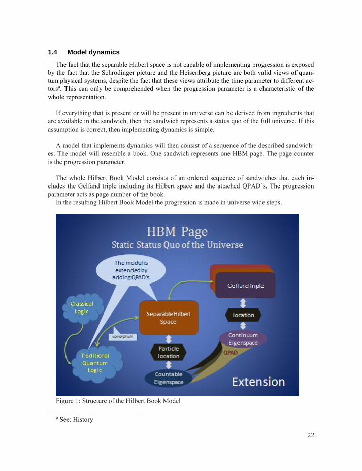
The whole Hilbert Book Model consists of an ordered sequence of sandwiches that each in-
cludes the Gelfand triple including its Hilbert space and the attached QPAD’s. The progression
parameter acts as page number of the book.
In the resulting Hilbert Book Model the progression is made in universe wide steps.
Figure 1: Structure of the Hilbert Book Model
9 See: History

23
24
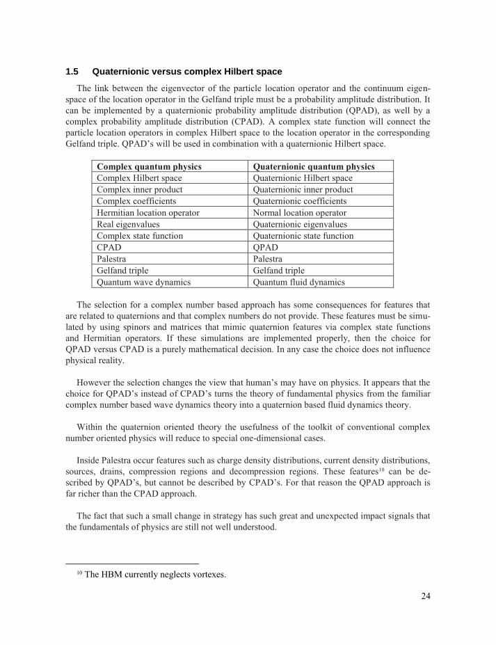
1.5 Quaternionic versus complex Hilbert space
The link between the eigenvector of the particle location operator and the continuum eigen-
space of the location operator in the Gelfand triple must be a probability amplitude distribution. It
can be implemented by a quaternionic probability amplitude distribution (QPAD), as well by a
complex probability amplitude distribution (CPAD). A complex state function will connect the
particle location operators in complex Hilbert space to the location operator in the corresponding
Gelfand triple. QPAD’s will be used in combination with a quaternionic Hilbert space.
Complex quantum physics Quaternionic quantum physics
Complex Hilbert space Quaternionic Hilbert space
Complex inner product Quaternionic inner product
Complex coefficients Quaternionic coefficients
Hermitian location operator Normal location operator
Real eigenvalues Quaternionic eigenvalues
Complex state function Quaternionic state function
CPAD QPAD
Palestra Palestra
Gelfand triple Gelfand triple
Quantum wave dynamics Quantum fluid dynamics
The selection for a complex number based approach has some consequences for features that
are related to quaternions and that complex numbers do not provide. These features must be simu-
lated by using spinors and matrices that mimic quaternion features via complex state functions
and Hermitian operators. If these simulations are implemented properly, then the choice for
QPAD versus CPAD is a purely mathematical decision. In any case the choice does not influence
physical reality.
However the selection changes the view that human’s may have on physics. It appears that the
choice for QPAD’s instead of CPAD’s turns the theory of fundamental physics from the familiar
complex number based wave dynamics theory into a quaternion based fluid dynamics theory.
Within the quaternion oriented theory the usefulness of the toolkit of conventional complex
number oriented physics will reduce to special one-dimensional cases.
Inside Palestra occur features such as charge density distributions, current density distributions,
sources, drains, compression regions and decompression regions. These features10 can be de-
scribed by QPAD’s, but cannot be described by CPAD’s. For that reason the QPAD approach is
far richer than the CPAD approach.
The fact that such a small change in strategy has such great and unexpected impact signals that
the fundamentals of physics are still not well understood.
10 The HBM currently neglects vortexes.
25
The HBM approach is also richer than the GRT approach. With respect to GRT, the HBM of-
fers a much more detailed analysis of what happens in the undercrofts of physics.
The implementation of physical fields via the attachment of QPAD’s to eigenvectors in the
separable Hilbert space is a crucial departure from conventional physical methodology. Conven-
tional quantum physics uses complex probability amplitude distributions (CPAD’s), rather than
QPAD’s11. Quantum Field Theory12, in the form of QED13 or QCD14, implements physical fields
in a quite different manner.
1.6 Advantages of QPAD’s
The choice for QPAD’s appears very advantageous. The real part of the QPAD can be inter-
preted as a “charge” density distribution. Similarly the imaginary part of the QPAD can be inter-
preted as a “current” density distribution. The squared modulus of the value of the QPAD can be
interpreted as the probability of the presence of the carrier of the “charge”. The “charge” can be
any property of the carrier or it represents a collection of the properties of the carrier. In this way,
when the state function is represented by a QPAD the equation of motion becomes a continuity
equation15.
Since the state function QPAD’s attach Hilbert eigenvectors to a value in a continuum the car-
riers can be interpreted as tiny patches of that continuum. The transport of these patches can be re-
sponsible for the local compression or decompression of the continuum space. With other words,
via this mechanism QPAD’s may influence the local curvature.
Interpreting the carriers as tiny patches of the parameter space is a crucial step. It transfers the
dynamics into quantum fluid dynamics. Only via this step it becomes possible that QPAD’s influ-
ence local curvature.
All state function QPAD’s share their parameter space. The shared parameter space is called
Palestra. This space can be curved. It can be represented by a quaternionic distribution. This qua-
ternionic distribution has a flat parameter space.
11 http://en.wikipedia.org/wiki/Probability_amplitude
12 http://en.wikipedia.org/wiki/Quantum_field_theory 13 http://en.wikipedia.org/wiki/Quantum_electrodynamics 14 http://en.wikipedia.org/wiki/Quantum_chromodynamics 15 Also called balance equation.
26
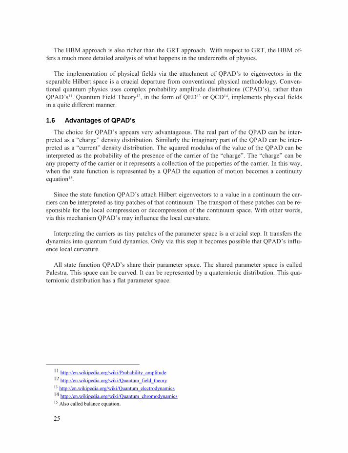
1.7 Sign flavors
In most cases where quaternionic distributions are used, the fact that quaternions possess two
independent types of sign selections is ignored. The first sign
selection type, the conjugation, inverts the sign of all three im-
aginary base vectors. It is a combination of the sign switch of
the whole number and the sign switch of the real part. The se-
cond sign selection type, the reflection, inverts the sign of a
single imaginary base vector. The reflection can be taken in
three independent directions. When relevant these directions
are color coded. The sign selections in a quaternionic distribu-
tion are all similar. Individually, the conjugation and the reflec-
tion switch the handedness of the external vector product in the
product of two quaternions that are taken from the same qua-
ternionic distribution. The sign selection of the parameter space
is usually taken as the reference for the sign selections of the
quaternionic distributions. When a quaternionic distribution has
the same sign selection as its parameter space has, then it will
be called a base quaternionic distribution.
For each QPAD, the mixture of conjugation and colored re-
flections produces eight different sign flavors16. This adds a
significant amount of functionality to quaternionic distribu-
tions. In quantum physics the sign flavors play a crucial role. In
conventional physics this role is hidden in complex probability
amplitude distributions (CPAD’s), alpha, beta and gamma ma-
trices and in spinors.
1.8 Virtual carriers and interactions
Primary QPAD’s are quaternionic distributions of the probability of presence of virtual
“charge” carriers. They have no other geometrical significance than that they are tiny patches of
the parameter space. The “charge” may stand for an ensemble of properties. Both state function
QPAD’s as well as constructed background QPAD’s are primary QPAD’s
The couplings of primary QPAD’s result in elementary particles17. The properties that charac-
terize this coupling form the sources of second category physical fields. Second category physical
fields have actual charges as their sources and particles as their charge carriers. Second category
physical fields concern a single property of the carrier. They are known as the physical field that
relates to that property. Their presence can be observed (detected).
16 R, G, B are colors. N is normal. W is white. L is left handed. R is right handed. 17 See: Particle physics
Figure 2: Sign selections
27
The Hilbert Book Model does not use the notion of a virtual particle. Instead the role of prima-
ry QPAD’s is used for this purpose.
Static primary QPAD's cannot be observed directly. Their existence can only be derived from
the existence of second category physical fields.
In the Hilbert Book Model the “implementation” of forces via the exchange of virtual particles
is replaced by the mutual influencing of the corresponding QPAD’s. This influence is instantiated
via the fact that the concerned primary QPAD’s superpose and that their currents feed/supply oth-
er QPAD’s.
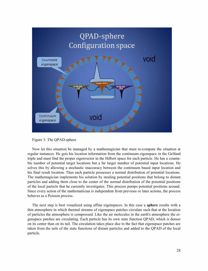
1.9 QPAD-sphere
QPAD's are quaternionic amplitude distributions and can be interpreted as a combination of a
scalar "charge" density distribution and a vectorial "current" density distribution. The currents in a
static QPAD consist of uniformly moving charge carriers. When the state function of a particle is
represented by a primary QPAD, then this gives a special interpretation of that state function. A
very special kind of primary QPAD is a local background QPAD18. It represents the local super-
position of the tails of the state functions of a category of distant elementary particles.
The QPAD's that act as state functions may be imagined in a region that glues the eigenspace
of the location operator that resides in the Gelfand triple to the Hilbert eigenvectors of the particle
location operator that resides in the separable Hilbert space. Constructed QPAD’s such as the
background QPAD’s also reside in this region. They may be coupled to state function QPAD’s. In
that case the coupling generates a particle. This region is called the QPAD-sphere and contains
potential “streams” of space patches that are superfluous in the eigenspace in the Gelfand triple
and that fail in the corresponding eigenspace in the separable Hilbert space. Both eigenspaces are
considered to be affine spaces. The actual streaming takes place in Palestra. Coupled QPAD’s act
as pumps that circulate space patches in the QPAD-sphere19.
18 See: Special QPAD’s 19 See: figure 3, the QPAD-sphere
28
Figure 3: The QPAD-sphere
Now let this situation be managed by a mathemagician that must re-compute the situation at
regular instances. He gets his location information from the continuum eigenspace in the Gelfand
triple and must find the proper eigenvector in the Hilbert space for each particle. He has a counta-
ble number of potential target locations but a far larger number of potential input locations. He
solves this by allowing a stochastic inaccuracy between the continuum based input location and
his final result location. Thus each particle possesses a normal distribution of potential locations.
The mathemagician implements his solution by stealing potential positions that belong to distant
particles and adding them close to the center of the normal distribution of the potential positions
of the local particle that he currently investigates. This process pumps potential positions around.
Since every action of the mathematician is independent from previous or later actions, the process
behaves as a Poisson process.
The next step is best visualized using affine eigenspaces. In this case a sphere results with a
thin atmosphere in which thermal streams of eigenspace patches circulate such that at the location
of particles the atmosphere is compressed. Like the air molecules in the earth's atmosphere the ei-
genspace patches are circulating. Each particle has its own state function QPAD, which is denser
on its center than on its tail. The circulation takes place due to the fact that eigenspace patches are
taken from the tails of the state functions of distant particles and added to the QPAD of the local
particle.
29
A coupled local state function pumps space patches taken from the tails of other state functions
to the drain at its center and supplies them to a background QPAD, which spreads them over its
surround. In this way it reclaims space patches that were supplied by distant sources and supplies
them in the form of local space patches. Thus the local background QPAD acts as a source where
the local coupled state function acts as a drain of space patches. The process that does this can be
characterized as a Poisson process. The result of the stream of space patches is a local space cur-
vature.

30
1.10 The HBM Palestra
We introduce a special kind of space. This space can curve. Its curvature can change. So, the
space can move. It is space that moves with respect to a coordinate system. If you attach a sepa-
rate coordinate system to the moving space, then you can describe what is happening. For exam-
ple it can be described by a quaternionic distribution. Use only the imaginary part of the values
and the imaginary part of the parameter. Now you have a distribution that describes your special
space. You can use this space as the parameter space of still another function. For example you
can use it as parameter space of a CPAD or a QPAD or any other field.
In the Hilbert Book Model all state function QPAD’s and the fields that are derived from them
or from their couplings, share the same parameter space. For that reason this common parameter
space will be given a special name; the HBM Palestra20. This shared parameter space spreads
universe wide. It is the place where universe is located.
The HBM Palestra does not correspond to the historic notions of ether21 that were used in phys-
ics. Instead it is defined by the descriptions that are given in this section.
In general QPAD’s are no more than special kinds of quaternionic distributions. In the HBM
some of the primary QPAD’s have a special interpretation as state functions of elementary parti-
cles. In the HBM CPAD’s will also use the HBM Palestra as their parameter space. If they are
used as state functions, then the Hilbert space will use complex numbers for its inner product.
CPAD’s are especially suited to handle one dimensional or one parametric problems.
The parameter space of a QPAD can be interpreted as a quaternionic distribution. It has itself a
parameter space, which is formed by a flat 3D continuum. The Palestra is taken from the eigen-
space of a location operator that resides in the Gelfand triple of the separable Hilbert space. Only
the imaginary part of the quaternionic distribution is used. It can be considered as a 3D Riemanni-
an manifold. The local metric defines the local curvature. What occurs in this manifold is de-
scribed by the QPAD’s. It is also possible to use the real part of the Palestra. However, in that
case the value represents the progression parameter and is a constant throughout the imaginary
part of the Palestra.
The Palestra is the playground of all what happens in fundamental physics. It is governed by a
special kind of fluid dynamics (QFD). Things like charge density distributions, current density
distributions, sources, drains, compressed regions and decompressed regions occur in this space.
The QPAD's are not the transporters. They only describe the transport process. The action takes
place in their shared parameter space, which is the Palestra. That’s how these QPADS’s can influ-
ence each other.
1.11 Dynamics control
What happens in Palestra can be distinguished in two types of dynamics;
the dynamics of particles and
the dynamics of fields.
20 The name Palestra is suggested by Henning Dekant’s wive Sarah. It is a name from Greek
antiquity. It is a public place for training or exercise in wrestling or athletics 21 http://en.wikipedia.org/wiki/Aether_theories
31
The dynamics of particles is controlled by quantum mechanics. The dynamics of fields is con-
trolled by quantum fluid dynamics.
1.11.1 Quantum mechanics
Quantum mechanics is well treated by conventional quantum physics. It concerns movements
of particles and oscillations of particles or oscillations inside conglomerates. It is usually treated
in the realm of a complex Hilbert space. The typical governing equation is the Schrödinger equa-
tion.
1.11.2 Quantum fluid dynamics
Quantum fluid dynamics relies on the use of QPAD’s as state functions. It concerns move-
ments of fields. It is treated in the realm of a quaternionic Hilbert space. The typical governing
equation is an equivalent of the quaternionic format of the Dirac equation. The generic equation is
the elementary coupling equation and it is best interpreted as balance equation.
What happens in the HBM Palestra is controlled by Quantum Fluid Dynamics (QFD). QFD
differs from conventional fluid dynamics in that in QFD the charge density distributions and cur-
rent density distributions describe probable locations and paths in their own parameter space,
while in conventional fluid dynamics these distributions describe actual locations and paths that
occur in an considered medium such as a gas or liquid. That is why in QFD the charge density
distributions and current density distributions are combined in quaternionic probability amplitude
distributions, while in conventional fluid dynamics they are located in scalar and vector fields.
1.11.3 Elementary coupling
Elementary coupling forms the base of particle generation. The elementary coupling equation
couples two QPAD’s ψ and φ.
φ
Here is the quaternionic nabla and is a coupling factor.
This equation immediately delivers a formula for the coupling factor .
∫ φ
∫ φ φ
When compared to the Dirac equation and the Majorana equation the two QPAD’s are sign
flavors of the same basic QPAD. With eight sign flavors for each QPAD, this results in 64 differ-
ent elementary coupling equations22. However, when φ it can be shown that must be zero.
In that case the QPAD must either be zero or it must oscillate.
Thus the restricted elementary coupling equation results in 56 particles and 8 waves. The parti-
cles are attached to an eigenvector of the (particle) location operator and the waves are attached to
an eigenvector of the canonical conjugate of the (wave) location operator.
22 See table of elementary particles.
(1)
(2)
32
In many cases the generated particles can be attributed to members of the standard model.
However, the standard model shows generations that do not yet show in this simple model. It
means that there are three versions of m or with other words there are three generations of the pair
{ }. It might be that the restriction that ψ and φ are sign flavors of the same base QPAD is too strong.
The elementary coupling provides the generated particle with four properties:
The coupling factor m
An electric charge
A spin
A color charge
In higher order couplings the first three properties are preserved. In fact these properties are
sources of new fields. All color charges appear to combine to white. Higher order couplings
couple elementary particles with each other and with fields.
1.12 Fields
In the HBM fields consist of
1. Oscillating QPAD’s (waves)
2. Fields coupled in elementary particles
a. State function QPAD’s
b. Constructed background QPAD’s
3. Coupling property fields
This leads to two categories of physical fields
Oscillating QPAD’s (waves)
Coupling property fields
33
2 History
In its first years, the development of quantum physics occurred violently. Little attention was
paid to a solid and consistent foundation. The development could be characterized as delving in
unknown grounds. Obtaining results that would support applications was preferred above a deep
understanding of the fundamentals.
The first successful results were found by Schrödinger and Heisenberg. They both used a quan-
tization procedure that converted a common classical equation of motion into a quantum mechan-
ical equation of motion. Schrödinger used a state function that varied as a function of its time pa-
rameter, while operators do not depend on time. Heisenberg represented the operators by matrices
and made them time dependent, while their target vectors were considered to be independent of
time. This led to the distinction between the Schrödinger picture and the Heisenberg picture.
Somewhat later John von Neumann and others integrated both views in one model that was
based on Hilbert spaces. Von Neumann also laid the connection of the model with quantum logic.
However, that connection was ignored in many of the later developments. Due to the restrictions
that are posed by separable Hilbert spaces, the development of quantum physics moved to other
types of function spaces. The Hilbert Book Model chooses a different way. It keeps its reliance on
quantum logic, but attaches fields, including state functions, in the region between the Hilbert
space and its Gelfand triple.
Due to the integration of both pictures in a single Hilbert space, it becomes clear that the
Schrödinger picture and the Heisenberg picture represent two different views of the same situa-
tion. It appears to be unimportant were time is put as a parameter. The important thing is that the
time parameter acts as a progression indicator. This observation indicates that the validity of the
progression parameter covers the whole Hilbert space. With other words, the Hilbert space itself
represents a static status quo. Conventional quantum physics simply ignores this fact.
In those days quaternions played no role. The vector spaces and functions that were used all
applied complex numbers and observables were represented with self-adjoint operators. These
operators are restricted to real eigenvalues.
Quaternions were discovered by the Irish mathematician Sir William Rowan Hamilton23 in
1843. They were very popular during no more than two decades and after that they got forgotten.
Only in the sixties of the twentieth century, supported by the discovery of Constantin Piron that a
separable Hilbert space ultimately may use quaternions for its inner product, a short upswing of
quaternions occurred. But quickly thereafter they fell into oblivion again. Currently most scien-
tists never encountered quaternions. The functionality of quaternions is taken over by complex
numbers and a combination of scalars and vectors and by a combination of Clifford algebras,
Grassmann algebras, Jordan algebras, alpha-, beta- and gamma-matrices and by spinors. The
probability amplitude functions were taken to be complex rather than quaternionic. Except for the
quaternion functionality that is hidden in the α β γ matrices, hardly any attention was given to the
23 http://en.wikipedia.org/wiki/William_Rowan_Hamilton
34
possible sign selections of quaternion imaginary base vectors and as a consequence the sign fla-
vors of quaternionic distributions stay undetected. So, much of the typical functionality of quater-
nions still stays obscured.
The approach taken by quantum field theory departed significantly from the earlier generated
foundation of quantum physics that relied on its isomorphism with quantum logic. Both QED and
QCD put the quantum scene in non-separable function spaces. The state function is only seen as a
complex probability amplitude distribution. Spinors and gamma matrices are used to simulate
quaternion behavior. Physical fields are commonly seen as something quite different from state
functions. However they are treated in a similar way.
The influence of Lorentz transformations gives scientists the impression that space and time do
not fit in a quaternion but instead in a spacetime quantity that features a Minkowski signature.
Length contraction, time dilation and space curvature have made it improbable that progression
would be seen as a universe wide parameter.
These developments cause a significant deviation between the approach that is taken in con-
temporary physics and the line according which the Hilbert Book Model is developed.
2.1 Criticism
Due to its unorthodox approach and controversial methods the Hilbert Book Model has drawn
some criticism
2.1.1 Model
Question:
The separable Hilbert space has clearly some nasty restrictions. Why can quantum physics not
be completely done in the realm of a rigged Hilbert space?
Answer:
In that case there is no fundamental reason for a separate introduction of fields in QP. It will al-
so not be possible to base QP on traditional quantum logic (TQL), because the isomorphism that
exists between TQL and separable Hilbert spaces (SHS’s) does not exist between TQL and a
rigged Hilbert space (RHS). See figure 1.
In the HBM the quaternionic probability amplitude distributions (QPAD’s) on which fields are
based, link the SHS with its Gelfand triple {Φ;SHS;Φ’}, which is a RHS. However, the QPAD’s
are not part of the SHS and are not part of the RHS. The HBM can be pictured as:
TQL⇔SHS⇒{QPAD’s}⇒RHS≡{Φ;SHS;Φ’}
The isomorphism ⇔ is replaced by incongruence ⇐≠⇒ in
TQL⇐≠⇒RHS
2.1.2 Quaternions
Remark1:
(1)
(2)
35
A tensor product between to quaternionic Hilbert spaces cannot be constructed. So it is better
to stay with complex Hilbert spaces.
Remark2:
The notion of covariant derivative, which is an important concept on quantum field theory, of-
fers problems with quaternionic distributions, so it is better to stay with a complex representation.
This is due to the fact that for quaternionic distributions in general24:
≠
Response:
The HBM proves that solutions exist that do not apply tensor products or covariant derivatives.
In fact the subject can be reversed:
If a methodology is in conflict with a quaternionic approach, then it must not be applied as a
general methodology in quantum physics. A complex number based method can best be applied in
special, one dimensional or one parametric cases.
2.1.3 Quaternionic versus complex probability amplitude distributions
Remark 1
Conventional physics solves everything by using complex probability amplitude distributions
(CPAD’s).
Remark 2
It is sufficient to stay with that habitude. Quaternionic probability amplitude distributions
(QPAD’s) might be unphysical.
Response:
QPAD’s extend the functionality of CPAD’s and make it possible to interpret equations of mo-
tion as balance equations. They can be considered as a combination of a scalar potential and a
vector potential or as the combination of a charge density distribution and a current density distri-
bution.
Their sign flavors enable the interpretation of spinors as a set of sign flavors that belong to the
same base QPAD. This throws new light on the Dirac and Majorana equations.
Coupling of QPAD’s can be related to local curvature. This interpretation is impossible with
CPAD’s.
2.2 Consequence
The application of the HBM requests from physicists that they give up some of the conven-
tional methodology and learn new tricks.
The HBM allows using complex number based quantum physics aside quaternion based quan-
tum physics. It introduces fields as objects that are separated from the separable Hilbert space as
well as from the corresponding Gelfand triple.
24 The quaternionic nabla can be split in its parts see below: Differentiation
(1)
36
PART II The Hilbert Book Model
37
3 INGREDIENTS
The most intriguing ingredients of the model are quaternions, quaternionic distributions and
quaternionic probability amplitude distributions (QPAD’s), both equipped with their sign flavors.
3.1 Role of the particle locator operator
The particle locator operator 𝔖 is one of the operators for which the eigenvectors are coupled
to a continuum called Palestra that is related to the eigenspace of a corresponding location opera-
tor that resides in the Gelfand triple.
Palestra may be curved. It means that this continuum is a quaternionic function of the eigen-
values of another location operator. The eigenspace of that operator is flat. It is covered by the
number space of the quaternions. Palestra has the same sign flavor as this parameter space. With-
out curvature its parameters and the corresponding values are equal.
For each eigenvector of the particle locator operator Palestra acts as parameter space for the
QPAD that connects this eigenvector with the eigenspace of the corresponding location operator
that resides in the Gelfand triple. It means that Palestra is identical with that eigenspace. The
QPAD can be visualized as a fuzzy funnel that drops stochastically inaccurate observation values
onto the particle.
The particle location operator has a canonical conjugate, which is the corresponding particle
momentum operator. This corresponds to a different particle eigenvector, a different QPAD, a dif-
ferent corresponding eigenspace in the Gelfand triple and a different corresponding operator. For
example the parameter space of the new QPAD is the canonical conjugate of Palestra and the cor-
responding momentum operator in the Gelfand triple is the canonical conjugate of the discussed
location operator. Without any curvature the old and the new QPAD would be each other’s Fouri-
er transform.
3.2 QPAD’s
All elementary particles correspond to different eigenvectors of the particle locator operator 𝔖. Each elementary particle has its own QPAD that acts as its state function.
Taken over a set of subsequent page numbers two pictures are possible. In both pictures exist-
ing particles are characterized by their own state function QPAD. Thus for particles their state
function QPAD is a stable factor.
According to the Heisenberg picture the QPAD is static between subsequent HBM pages, but
links to different eigenvectors of the particle location operator.
According to the Schrödinger picture the QPAD varies between subsequent HBM pages, but
links to the same eigenvector of the particle location operator.
In both pictures a location observation must deliver the same result.
If we want to categorize particles, then we must categorize their state function QPAD’s.
But, we also must take the background QPAD in account to which the state function QPAD is coupled.
38
Some QPAD’s stay uncoupled. These QPAD’s must oscillate25. They form elementary waves. All elementary waves correspond to different eigenvectors of the wave locator operator
��, which is the canonical conjugate of 𝔖. If a QPAD has a well-defined location in configuration space, then it does not have a well-
defined location in the canonical conjugate space. So for this investigation we better consid-er both locations together.
A possible strategy is to use the superposition of the QPAD and its Fourier transform. This solution distinguishes QPAD’s that, apart from a scalar, are invariant under Fourier transformation26.
An important category of invariants is formed by QPAD’s that have the shape , where is a constant and is the distance from the central location2728.
Further it is sensible to introduce for each category the notion of an average QPAD. De-termining the average QPAD either involves integration over full Palestra or it involves inte-gration over the canonical conjugate of Palestra.
Another procedure constructs the superposition of all tails of a category of QPAD’s at a certain location. This produces a background QPAD. For each location such a background QPAD exists, but it may differ per location. However, when a large category is involved, it can only differ very marginally for neighboring locations.
3.3 Helmholtz decomposition
A static QPAD consists of a charge density distribution and an independent current density dis-
tribution. The charge density distribution corresponds to a curl free vector field and the current
density distribution corresponds to a divergence free vector field. Any change in the currents goes
together with extra field components that do not correspond to the charge density distribution or
the current density distribution.
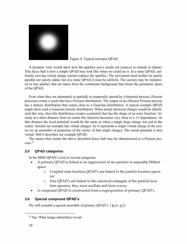
3.4 QPAD vizualization
If I was a good artist and I was asked to give an artist impression of the magic wand of a magi-
cian, then I would not paint a dull rod or a stick with a star at the end. Instead I would draw a very
thin glass rod that has a sparkling fuzzy ball at its tip. A static view of that ball would be like:
25 See Free QPAD’s 26 See Appendix; Functions invariant under Fourier transform 27 http://en.wikipedia.org/wiki/Hankel_transform#Some_Hankel_transform_pairs 28 Also see http://en.wikipedia.org/wiki/Bertrand's_theorem
39
Figure 4: Typical isotropic QPAD
A dynamic view would show how the sparkles move inside out (source) or outside in (drain).
This fuzzy ball is how a simple QPAD may look like when we could see it. In a static QPAD, uni-
formly moving virtual charge carriers replace the sparkles. The movement need neither be purely
parallel nor purely radial, but in a static QPAD it must be uniform. The carriers may be interpret-
ed as tiny patches that are taken from the continuum background that forms the parameter space
of the QPAD.
Even when they are attenuated or spatially or temporally spread by a binomial process, Poisson
processes create a result that has a Poisson distribution. The output of an efficient Poisson process
has a density distribution that comes close to a Gaussian distribution. A typical example QPAD
might show such a Gaussian density distribution. When actual electrical charges would be distrib-
uted this way, then this distribution creates a potential that has the shape of an error function. Al-
ready at a short distance from its center this function decreases very close to a 1/r dependence. At
that distance the local potential would be the same as when a single large charge was put at the
center. Instead our example has virtual charges. So it represents a single virtual charge at the cen-
ter (or an ensemble of properties of the carrier of that single charge). The raised potential is also
virtual. Still it describes our example QPAD.
The source that creates the above described fuzzy ball may be characterized as a Poisson pro-
cess.29
3.5 QPAD categories
In the HBM QPAD’s exist in several categories:
A primary QPAD is linked to an eigenvector of an operator in separable Hilbert
space.
o Coupled state function QPAD’s are linked to the particle location opera-
tor
o Free QPAD’s are linked to the canonical conjugate of the particle loca-
tion operator, they must oscillate and form waves.
A composed QPAD is constructed from a superposition of primary QPAD’s
3.6 Special composed QPAD’s
We will consider a special ensemble of primary QPAD’s { ψ }.
29 See: What image intensifiers reveal
40
The ψ are normalized: ∫ |ψ |
.
The ψ must be spherically symmetric.
From a given minimal distance their modulus must decrease with radius as
.
The special composed QPAD’s are Fourier transform invariant and conform to Bertrand’s the-
orem30.
3.6.1 The average QPAD
The ensemble { ψ } of the special composed QPAD’s has an average
3.7 The background QPAD
Background QPAD’s are composed QPAD’s. A given background QPAD depends on the se-
lection criterion that is used in the composition. Every sign flavor might have its own background
QPAD.
The ensemble { ψ } is distributed randomly over the center points { } in an affine param-
eter space. At a given point P in this space the superposition of all tails of the members of the en-
semble { ψ } will be constructed.
This superposition will be renormalized and then indicated by Φ . Thus,
∫|Φ |
In this superposition the largest contribution comes from the ψ for which the is farthest
from P. Further the directions of the imaginary part are reversed with respect to the directions in
the ψ . Especially at long distances, all differences are smoothed away via an averaging process.
The result is that for a background QPAD that consist of the superposition of the tails of all
QPAD’s in universe:
Φ =
We will interpret Φ as the background QPAD.
The approach taken here, shows similarity with the approach of Denis Sciama in his paper:
“On the origin of inertia”31.
3.7.1.1 Uniform movement
Due to its construction the location as well as the shape of the background QPAD is very sta-
ble. In the HBM the background QPAD is reconstructed at every subsequent page. As long as the
30 http://en.wikipedia.org/wiki/Bertrand%27s_theorem 31 See: http://www.adsabs.harvard.edu/abs/1953MNRAS.113...34S
(1)
(2)
41
whole QPAD remains static, it can be reconstructed at a displaced location. Thus, as long as this
movement is contained in its current density distribution, the background QPAD can move freely
in a uniform way.
In principle every location has its own background QPAD. However, it makes only sense to
couple the locations of particles with a local background QPAD. If this coupling is strong then it
acts as a sticky resistance against acceleration of the coupled particle.
3.7.2 Isotropy
Source QPAD’s are isotropic. Drain QPAD’s are also isotropic and are the conjugate of a cor-
responding source QPAD.
Anisotropic QPAD’s are hybrids. In one or two dimensions they correspond to source
QPAD’s. In the other dimensions they correspond to a drain QPAD.
Oscillating QPAD’s oscillate between source modes and drain modes. They usually can be de-
scribed by spherical or linear harmonic (quantum) oscillators. A special case of the oscillating
QPAD is a plain wave.
3.8 Physical fields
Physical fields appear in two categories32
The first category physical field concerns free primary QPAD’s.
The second category physical field relate to properties of coupled QPAD’s
Each of the members of the second category of physical fields represents the influences of a
single property of a coupled pair of QPAD’s.
The two categories are fundamentally different. They behave differently33.
3.9 Inertia
Inertia34 is based on the fact that all particles in universe influence a selected local particle.
Since this influence is isotropic it usually does not disturb the particle. This condition holds as
long as the particle is located stationary or moves uniformly. In that case the connected QPAD is
static. However, when the particle accelerates, according to field theory, this goes together with
the existence of an extra field that becomes part of the particle’s QPAD and that counteracts the
acceleration.
The background QPAD that is coupled to the state function QPAD at the right side of the ele-
mentary coupling equation35 represents the influence of the universe on the local particle. It repre-
sents the superposition of all tails of a category of state functions of particles that exist in uni-
verse. For that reason it is the source of inertia. This is shown in the elementary coupling
equation.
32 For more details see chapter 4. 33 This becomes apparent at the event horizon of black holes. 34 Appendix; The universe of items 35 See Elementary particles
42
For the restricted elementary coupling equation the QPAD’s and are sign flavors of the
same base QPAD , which on its turn has the same sign flavor as Palestra has.
For elementary fermions the coupled field equals the isotropic background field Φ.
For electrons the state function equals Φ The formula (1) holds for all massive elementary particle types. It holds for elementary fermi-
ons as well as for the elementary bosons that couple to other sign flavors36 than Φ.
If the restricted elementary coupling equation holds then, for every QPAD sign flavor that
acts as a state function of an elementary particle, exists a background QPAD 37 that has the
same base QPAD . The corresponding particle type is fully characterized by the pair { } These facts are in detail treated in the section on particle physics.
According to equation (1) the state function QPAD is rather strongly coupled to the local back-
ground QPAD. The equation describes the situation of an independently moving particle.
In atoms the electrons oscillate around the nucleus. There these particles move more freely.
They are still coupled to the centrally located background QPAD, but the coupling is rather loose.
Equation (1) does not describe that situation. Instead of the Dirac equation, the Klein-Gordon
equation fits more appropriately.
The background QPAD’s play the role that is thought for the Higgs field.
3.10 Coupling and curvature
When a local state function QPAD is coupled to a local background QPAD, then the back-
ground QPAD can be considered as a source that supplies space patches to the local state function
QPAD. On its turn the local state function QPAD acts as a drain. Thus, the coupled system pumps
space taken from the rest of the universe to the location of the local state function QPAD. These
flowing space patches form part of the space that the eigenspace of the location operator that
resides in the Gelfand triple has extra with respect to the eigenspace of the particle location
operator that resides in the separable Hilbert space. Otherwise said: the eigenspace compresses
via the state function QPAD to the eigenspace and expands back via the coupled background
QPAD to eigenspace . The observer that uses as his observation space, experiences a local
compression of his observation space at the location of the observed QPAD. This can be ex-
pressed by a local curvature of the observation space.
As extra detail can be said that the source and the drain act as Poisson processes that cause a
Gaussian distribution of the patches of space that flow in/out the drain/source location.
The moving space patches may be interpreted as virtual carriers of the properties that charac-
terize the coupling event.
36 See Quaternions; Sign selections 37 See: the QPAD game
(1)

43
The coupling properties themselves act as sources of second category physical fields. These are
known as second category physical fields. In the GRT based Kerr-Newman metric equation38 sim-
ilar properties act as sources of curvature.
38 The Kerr-Newman equation is NOT part of the HBM. It is only used for comparison.
44
3.11 Hyper-complex numbers
Hyper-complex numbers form categories that are ordered with respect to their dimension. The
dimension takes the form , where is a non-negative integer. A hyper-complex number
of dimension can be obtained from a pair of hyper-complex numbers of dimension via a
construction algorithm. Several construction algorithms exist. The most popular is the Cayley-
Dickson construction39. A less known construction algorithm is the 2n-on construction of Warren
Smith40. This construction delivers numbers that in the higher dimensions retain better arithmetic
capabilities. Up and including the octonions the two construction algorithms deliver the same
numbers. The sedions differ from the 24-ons.
In their lower m dimensions the 2n-ons behave similarly to the 2
m-ons.
The 2n-ons have n independent imaginary base vectors. As a consequence the 2
n-ons feature n
independent sign selections or when independent directions are considered it are 2n independent
sign selections.
Both construction methods ignore these sign selections. Sign selections play a crucial role in
this paper.
3.12 Quaternions
A quaternion is a 1+3 dimensional hyper-complex number. It has a one dimensional real part
and a three dimensional imaginary part. As a result, it can be seen as the combination of a real
scalar and a three dimensional vector.
The quaternions form a division ring41. According to the Frobenius theorem42, the only finite-
dimensional division algebras over the reals are the reals themselves, the complex numbers, and
the quaternions.
The coefficients { } are real numbers. Bi-quaternions exist that have complex coefficients,
but these do not form a division ring.
3.12.1 Sign selections
The quaternions possess two independent sign selection types. When directions are reckoned
they constitute four independent sign selections. The conjugation ⇔ inverts the sign of all
imaginary base vectors. It acts isotropic.
39 http://en.wikipedia.org/wiki/Cayley%E2%80%93Dickson_construction 40 Appendix; 2
n-ons, See http://www.math.temple.edu/~wds/homepage/nce2.pdf
41 http://en.wikipedia.org/wiki/Division_ring 42 http://en.wikipedia.org/wiki/Frobenius_theorem_(real_division_algebras)
(1)
(1)
45
The reflection ⇔ inverts a single imaginary base vector and for
that reason it acts anisotropic.
Here, the base vector is selected arbitrarily.
The four sign selections can be mixed. They generate eight sign states.
Thus, if the three independent directions in which reflections can occur are also taken into ac-
count, then eight different sign selections are possible.
These sign selections are color coded as is shown in figure 2.
Individually the conjugation and the reflection both flip the handedness of the external vector
product of the imaginary part when both factors use the same sign selections.
(2)
46
3.12.2 Habits
The addition works as in all division rings, however the product of two quaternions does not
commute.
3.12.2.1 Product rule
The product rule is best expressed in the form of real scalars and 3D vectors:
⟨ ⟩
⟨ ⟩
3.12.2.2 Norm
The norm or modulus is defined by:
| | √ ⟨ ⟩
3.13 Quaternionic distributions
Several forms of quaternionic distributions exist. Two forms are relevant for the HBM.
A curved coordinate system can be related to a flat coordinate system via a quaternionic distri-
bution. The flat coordinate system plays the role of parameter space. On its turn the curved coor-
dinate system can also play the role of a parameter space. It does that for quaternionic probability
amplitude distributions (QPAD’s). In the HBM, Palestra is the parameter space that is shared by
all QPAD’s , all CPAD’s and all derived fields.
A quaternionic probability amplitude distribution 43 is a quaternionic distribution. Its value can
be split in a real part that can be interpreted as a charge density distribution and an imaginary part
that can be interpreted as a current density distribution. The squared modulus of the value can be
interpreted as the probability density of the presence of the carrier of the charge. The charge can
be any property of the carrier or it stands for the ensemble of the properties of the carrier.
43 http://en.wikipedia.org/wiki/Probability_amplitude treats complex probability amplitude dis-
tributions.
(1)
(2)
(3)
(4)
(5)
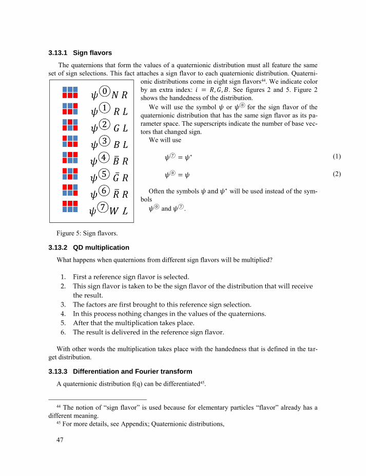
47
3.13.1 Sign flavors
The quaternions that form the values of a quaternionic distribution must all feature the same
set of sign selections. This fact attaches a sign flavor to each quaternionic distribution. Quaterni-
onic distributions come in eight sign flavors44. We indicate color
by an extra index: . See figures 2 and 5. Figure 2
shows the handedness of the distribution.
We will use the symbol or for the sign flavor of the
quaternionic distribution that has the same sign flavor as its pa-
rameter space. The superscripts indicate the number of base vec-
tors that changed sign.
We will use
Often the symbols and will be used instead of the sym-
bols
and .
Figure 5: Sign flavors.
3.13.2 QD multiplication
What happens when quaternions from different sign flavors will be multiplied?
1. First a reference sign flavor is selected.
2. This sign flavor is taken to be the sign flavor of the distribution that will receive
the result.
3. The factors are first brought to this reference sign selection.
4. In this process nothing changes in the values of the quaternions.
5. After that the multiplication takes place.
6. The result is delivered in the reference sign flavor.
With other words the multiplication takes place with the handedness that is defined in the tar-
get distribution.
3.13.3 Differentiation and Fourier transform
A quaternionic distribution f(q) can be differentiated45.
44 The notion of “sign flavor” is used because for elementary particles “flavor” already has a
different meaning. 45 For more details, see Appendix; Quaternionic distributions,
(1)
(2)
48
⟨ ⟩ ( )
The colored and signs refer to the influence of conjugation of on quaternionic multi-
plication. The sign refers to the influence of reflection of . In this section, the parameter q is supposed to be taken from a non-curved parameter space.
With that precondition, in Fourier space differentiation becomes multiplication with the canonical
conjugate coordinate and therefore the equivalent equation becomes:
g ⟨ ⟩ ( )
For the imaginary parts holds:
( )
( )
3.13.4 Spinors and matrices
In contemporary physics complex probability amplitude distributions (CPAD’s) are used rather
than QPAD’s. Spinors and matrices are used to simulate QPAD behavior for CPAD’s.
A spinor [ ] is a 1×4 matrix consisting of CPAD’s that represent the sign flavors of a QPAD. Sometimes the spinor is represented as a 1×2 matrix.
The and matrices influence the elements of spinor [ ].
[
]
[
]
[
]
[ ]
and represent imaginary base vectors of the simulated quaternion. represents the con-
jugation action for the spinor.
A relation exist between and the Pauli46 matrices :
46 http://en.wikipedia.org/wiki/Pauli_matrices
(1)
(2)
(3)
(4)
(3)
(4)
(5)
(6)
49
[ ] [
] [
]
This combination is usually represented in the form of gamma matrices.
In Dirac representation, the four contravariant gamma matrices are
[
] [
]
[
] [
]
It is useful to define the product of the four gamma matrices as follows:
[
]
The gamma matrices as specified here are appropriate for acting on Dirac spinors written in the
Dirac basis; in fact, the Dirac basis is defined by these matrices. In the Dirac basis47:
[
] [
] [
]
This corresponds with , .
Apart from the Dirac basis, a Weyl basis exists
[ ] [
] [
]
The Weyl basis has the advantage that its chiral projections48 take a simple form:
[ ] [
] [ ]
[ ] [
] [ ]
47 http://en.wikipedia.org/wiki/Gamma_matrices#Dirac_basis 48 http://en.wikipedia.org/wiki/Chirality_(physics)
(7)
(8)
(9)
(10)
(11)
(12)
(13)
(14)
50
[ ] [ ] [ ]
3.13.5 Continuity equation
When applied to a quaternionic probability amplitude distribution (QPAD), the equation for
the differentiation leads to a continuity equation49.
When is interpreted as a charge density distribution, then the conservation of the corre-
sponding charge50 is given by the continuity equation:
Total change within V = flow into V + production inside V
∫
∮
∫
∫
∫⟨ ⟩
∫
Here is the normal vector pointing outward the surrounding surface S, is the velocity
at which the charge density enters volume V and is the source density inside V. In the
above formula stands for
It is the flux (flow per unit area and unit time) of .
The combination of and is a quaternionic skew field and can be seen as
a probability amplitude distribution (QPAD).
can be seen as an overall probability density distribution of the presence of the
carrier of the charge. is a charge density distribution. is the current density distri-
bution.
The conversion from formula (2) to formula (3) uses the Gauss theorem51. This results in the
law of charge conservation:
⟨ ( )⟩
⟨ ⟩
⟨ ⟩ ⟨ ⟩
49 See: http://en.wikipedia.org/wiki/Reynolds_transport_theorem 50 Also see Noether’s laws: http://en.wikipedia.org/wiki/Noether%27s_theorem 51 http://en.wikipedia.org/wiki/Divergence_theorem
(15)
(1)
(2)
(3)
(4)
(5)
(6)
51
⟨ ⟩
The blue colored ± indicates quaternionic sign selection through conjugation of the field
. The field is an arbitrary differentiable vector function.
⟨ ⟩
is always divergence free. In the following we will neglect .
Equation (6) represents a balance equation for charge density. What this charge actually is, will
be left in the middle. It can be one of the properties of the carrier or it can represent the full en-
semble of the properties of the carrier.
This only treats the real part of the full equation. The full equation runs:
⟨ ⟩ ( )
⟨ ⟩ ⟨ ⟩
( )
⟨ ⟩ ⟨ ⟩
( ( ))
The red sign selection indicates a change of handedness by changing the sign of one of the im-
aginary base vectors. Conjugation also causes a switch of handedness. It changes the sign of all
three imaginary base vectors.
3.14 Hilbert space
The unit sphere of the separable Hilbert space Ң is an affine space. All unit size eigenvectors
end in this sphere.
A normal operator in the separable Hilbert space has set of unit size eigenvectors that span the
complete Hilbert space as an orthogonal base. For normal operators each eigenvector corresponds
to an eigenvalue.
This does not hold for the particle location operator and it also does not hold for the wave loca-
tion operator. The wave location operator is the canonical conjugate of the wave position opera-
(7)
(8)
(9)
(10)
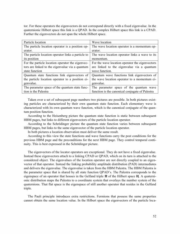
52
tor. For these operators the eigenvectors do not correspond directly with a fixed eigenvalue. In the
quaternionic Hilbert space this link is a QPAD. In the complex Hilbert space this link is a CPAD.
Further the eigenvectors do not span the whole Hilbert space.
Particle location Wave location
The particle location operator is a position op-
erator.
The wave location operator is a momentum op-
erator.
The particle location operator links a particle to
its position
The wave location operator links a wave to its
momentum.
For the particle location operator the eigenvec-
tors are linked to the eigenvalue via a quantum
state function
For the wave location operator the eigenvectors
are linked to the eigenvalue via a quantum
wave function.
Quantum state functions link eigenvectors of
the particle location operator to a position ei-
genvalue.
Quantum wave functions link eigenvectors of
the wave location operator to a momentum ei-
genvalue.
The parameter space of the quantum state func-
tion is the Palestra
The parameter space of the quantum wave
function is the canonical conjugate of Palestra
Taken over a set of subsequent page numbers two pictures are possible. In both pictures exist-
ing particles are characterized by their own quantum state function. Each elementary wave is
characterized with its own quantum wave function, which is the canonical conjugate of the quan-
tum position function.
According to the Heisenberg picture the quantum state function is static between subsequent
HBM pages, but links to different eigenvectors of the particle location operator.
According to the Schrödinger picture the quantum state function varies between subsequent
HBM pages, but links to the same eigenvector of the particle location operator.
In both pictures a location observation must deliver the same result.
According to this view the state functions and wave functions carry the post conditions for the
previous HBM page and the preconditions for the next HBM page. They control temporal conti-
nuity. This is best expressed in the Schrödinger picture.
The eigenvectors of the locator operators are exceptional. They do not have a fixed eigenvalue.
Instead these eigenvectors attach to a linking CPAD or QPAD, which on its turn is attached to the
considered object. The eigenvalues of the location operator are not directly coupled to an eigen-
vector of that operator. Instead the linking probability amplitude distribution (PAD) intermediates
and delivers the eigenvalue. The eigenvalue is taken from the HBM Palestra. The HBM Palestra is
the parameter space that is shared by all state function QPAD’s. The Palestra corresponds to the
eigenspace of an operator that houses in the Gelfand triple Ħ of the Hilbert space Ң. A quaterni-
onic distribution maps the Palestra to a coordinate system that overlays the number system of the
quaternions. That flat space is the eigenspace of still another operator that resides in the Gelfand
triple.
The Pauli principle introduces extra restrictions. Fermions that possess the same properties
cannot obtain the same location value. In the Hilbert space the eigenvectors of the particle loca-
53
tion operator that are attached to fermions are mutually orthogonal, but do not form a base of the
full Hilbert space.
When stepping from one HBM page to the next page, the state function QPAD’s install the
tendency to keep the corresponding eigenvectors together such that the corresponding expected
eigenvalues form a coherent and ordered set.
The coupling between the eigenvectors of the particle locator operator and the Palestra is not
precise. It is stochastic and its minimal size is of the order of the Planck-length. This granularity is
due to the fact that the Hilbert space is separable and as a consequence the set of eigenvalues is
countable. That is why the granules in the surface of a black hole have this size. The surface of a
black hole is an image of the unit sphere of a subspace of the Hilbert space where the eigenvectors
of the particle location operator form an orthogonal base and all attached QPAD’s pack the eigen-
values together in an optimal way.
Via the PAD, the eigenvectors of the particle locator operator all touch such a granule. The re-
lation with quantum logic means that the Hilbert vector stands for a proposition that has a yes/no
value. In case of the Hilbert vectors that are attached to the granules the yes/no value represents
group membership. Thus each granule represents a bit of information.
For the eigenvectors of the particle locator operator a densest packaging exists. It means that in
that condition the QPAD’s have shrunk to their smallest possible location difference.
54
4 PARTICLE PHYSICS
This chapter treats the first level coupling. The result of that coupling are first level particles.
These particles are solely created out of coupled primary QPAD’s and annihilate back into prima-
ry QPAD’s52. That is why these particles are called elementary particles. The zero-level of cou-
pling stands for no coupling. It results in elementary waves.
This section will not separate different particle generations.
4.1 Elementary coupling equation
First level particles appear to obey a special kind of continuity equation. The generic equation
is called the elementary coupling equation. In this continuity equation the source/drain term is
represented by the coupled background QPAD φ. It is coupled to the state function QPAD .
φ
Here is the quaternionic nabla and is a coupling factor.
This equation immediately delivers a formula for the coupling factor .
∫ φ
∫ φ φ
For the antiparticle holds the conjugated equation.
φ
Apart from the conjugation, it looks exactly the same equation as (1), but the Palestra does not
take part in the conjugation. In comparison with ”normal” elementary particles, the antiparticles
act as if progression is reversed.
4.2 Restricted elementary coupling
Restricted elementary coupling means that the coupled QPAD’s are sign flavors of the same
base QPAD. Both the Dirac equation and the Majorana equation belong to this type of elementary
coupling equation.
For all restricted particles hold:
⟨ ⟩
For the antiparticle:
52 In this chapter only QPAD’s are discussed. CPAD’s do not carry sign flavors.
(1)
(2)
(3)
(1)
(2)
(3)
55
The Fourier transform equivalents are
⟨ ⟩
is generally known as the Hamiltonian. is the momentum.
∫
∫ ;
The factor is real and non-negative.
Further, the equation for coupling factor is:
∫
∫
∫| |
An equivalent of the Lagrangian may look like
4.2.1 Dirac equation
The best known equation of motion for elementary fermions is the Dirac equation. It is written
using spinors and matrices.
The Dirac equation for a free moving electron or positron is known as:
[ ] [ ] [ ]
The Dirac matrices and give the spinor [ ] the function of a pair of QPAD’s.
This spinor equation can be converted into two quaternionic equations that act on the QPAD’s
and :
(4)
(5)
(6)
(7)
(8)
(9)
(10)
(1)
(2)
(3)
56
In the mass term the coupling factor couples and . When then and are
not coupled. Further:
In the left term of equations (2) and (3), and represent the state function of the particle.
In the right side appears the background field. In that sense { } and { } represent each
other’s antiparticle.
Reformulating these equations gives
For the conjugated equation holds
This implements the reverse flip. The corresponding particle is the antiparticle.
{ } { }
Both flips switch the handedness.
Equations (5) and (7) are each other’s quaternionic conjugate. However, it must be noticed that
all terms are conjugated, including the nabla operator, but the parameter space stays untouched.
Thus equation (7) differs from equation (5).
Summing the equations gives via
⟨ ⟩
the result
⟨ ⟩
The difference gives
Just reversing the sign flavors does not work. For the same QPAD , the corresponding equa-
tion will contain extra terms:
(4)
(5)
(6)
(7)
(8)
(9)
(10)
(11)
(12)
57
⟨ ⟩ ⟨ ⟩
⟨ ⟩
Thus if the reverse equation fits, then it will concern another QPAD configuration that will
not fit the original equation.
The pair { } that fits equation:
represents a different particle than the electron { }, which obeys equation (5). It also
differs from the positron { }, which obeys equation (7).
Where the electron couples to the general background QPAD , the new particle couples to
the conjugate of the general background QPAD . The new particle is called a shadow of
the positron.
4.2.1.1 The coupling factor
Multiplying both sides of the equation of motion for the electron:
with and then integrate over the full parameter space gives:
∫
∫
∫| |
Thus, the coupling factor can be computed from the QPAD .
4.2.2 The Majorana equation
The Majorana equation deviates from the Dirac equation in that is applies another sign flavor
of the state function QPAD . That other sign flavor is still coupled to the general background
QPAD .
The conjugated equation defines the antiparticle.
(13)
(14)
(1)
(2)
(1)
(2)
58
The particle is represented by the ordered pair { }. The corresponding flip does not
switch the handedness.
The Majorana equation is thought to hold for neutrinos, which are neutral. Equation (2) will
then hold for the anti-neutrino.
The coupling factor for the neutrino follows from:
∫
∫
∫| |
The pairs { }, { } and { } give similar results. They correspond to dif-
ferent colors (R,G,B) and to anti-neutrinos { }, { } and { }
4.2.3 The next particle type
We have exploited:
and
With equivalents { }, { } and { }.
The next possibility would be:
The conjugated equation is:
The particle is represented by the ordered pair { }. The corresponding flip does switch
the handedness. Again the state function QPAD is coupled to the general background QPAD .
Like the electron, this particle will have charge, but its charge will be three times lower, be-
cause only one instead of three imaginary base vectors cause the switch in handedness. Of course,
this is an opportunistic interpretation, but it seems to fit when we assume that the particle is a
down quark with charge equal to -⅓e.
The formula for the coupling factor is:
∫
∫
∫| |
(3)
(1)
(2)
(3)
(4)
(5)
59
The coupling that constitutes the down quark is anisotropic. This fact introduces a new kind of
charge, which is called color charge. The color is related to the direction of the reflection of the
state function QPAD.
The pairs { }, { } and { } give similar results. They represent the three
down quark colors. The corresponding antiparticles are { }, { } and { }.
In summary the down quarks have the following properties:
Location
o Position
o Momentum
Electric charge
Spin
Color charge
For down quarks the color charge is relevant. This is due to the fact that three down quarks
can combine in a baryon53. Without the existence of color charge the Pauli principle would
forbid that.
4.3 Massles bosons
This paragraph treats the zero-level of coupling.
4.3.1 No coupling
The last possible form in which the state function couples to the background field is:
The formula for the coupling factor is:
∫
∫
∫| |
∫
∫ | |
Presence does not leak. So,
.
With other words a QPAD does not couple to itself. What results is a free QPAD.
53 See: Hadrons
(1)
(2)
(3)
(4)
60
and deliver photons. The other sign flavors deliver gluons.
4.3.2 The free QPAD
When for sign flavor the coupling factor is zero then:
⟨ ⟩
It means that a change in the speed of the current goes together with a rotation of the
current
and/or a new field :
For comparison, in the equations of Maxwell54 the field is defined as:
In those equations is the electric field and is the magnetic field. However here these fields
have a more general meaning.
Thus equation (3) means:
More interesting is the corollary
⟨ ⟩
Thus
54http://en.wikipedia.org/wiki/Maxwell%27s_equations#Potential_formulation
(1)
(2)
(3)
(4)
(5)
(6)
(7)
(8)
(9)
(10)
61
Or
Further
⟨
⟩ ⟨ ⟩ ⟨ ⟩
Thus:
With other words a free (= not coupled) is either harmonic or it is static. The static condi-
tion corresponds to the ground state.
This holds for all QPAD’s.
4.3.2.1 Spin
Free QPAD’s have spin55.
∫
Elementary bosons appear to have the same value. It is not clear why in couplings this spin re-
duces to half this value for elementary fermions.
4.4 Consideration
We have now exhausted all possibilities for coupling a QPAD sign flavor to the general back-
ground QPAD . Above we could link the analyzed particles to electrons, neutrinos and down
quarks. Their antiparticles were treated as well. The investigated particles are elementary fermi-
ons. (We did not state or explain why they are fermions.)
We also analyzed the situation that a QPAD is coupled to itself. That situation leads to zero
coupling factor, which means no coupling. The free QPAD’s are bosons and correspond to pho-
tons or gluons. (We did not state or explain why these objects are bosons.)
The ordered pair {ψˣ, ψʸ } represents a category of elementary particle types.
For antiparticles all participating fields and the nabla operator conjugate.
We can now try to establish the apparent rules of the game. The rules are:
55 Bo Thidé: http://www.plasma.uu.se/CED/Book/EMFT_Book.pdf ,formula (4.76a)
(11)
(12)
(13)
(14)
(1)
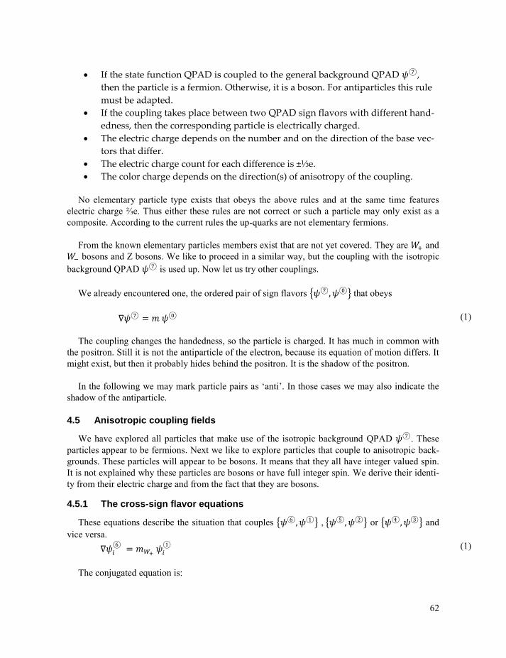
62
If the state function QPAD is coupled to the general background QPAD ,
then the particle is a fermion. Otherwise, it is a boson. For antiparticles this rule
must be adapted.
If the coupling takes place between two QPAD sign flavors with different hand-
edness, then the corresponding particle is electrically charged.
The electric charge depends on the number and on the direction of the base vec-
tors that differ.
The electric charge count for each difference is ±⅓e.
The color charge depends on the direction(s) of anisotropy of the coupling.
No elementary particle type exists that obeys the above rules and at the same time features
electric charge ⅔e. Thus either these rules are not correct or such a particle may only exist as a
composite. According to the current rules the up-quarks are not elementary fermions.
From the known elementary particles members exist that are not yet covered. They are and
bosons and Z bosons. We like to proceed in a similar way, but the coupling with the isotropic
background QPAD is used up. Now let us try other couplings.
We already encountered one, the ordered pair of sign flavors { } that obeys
The coupling changes the handedness, so the particle is charged. It has much in common with
the positron. Still it is not the antiparticle of the electron, because its equation of motion differs. It
might exist, but then it probably hides behind the positron. It is the shadow of the positron.
In the following we may mark particle pairs as ‘anti’. In those cases we may also indicate the
shadow of the antiparticle.
4.5 Anisotropic coupling fields
We have explored all particles that make use of the isotropic background QPAD . These
particles appear to be fermions. Next we like to explore particles that couple to anisotropic back-
grounds. These particles will appear to be bosons. It means that they all have integer valued spin.
It is not explained why these particles are bosons or have full integer spin. We derive their identi-
ty from their electric charge and from the fact that they are bosons.
4.5.1 The cross-sign flavor equations
These equations describe the situation that couples { } , { } or { } and
vice versa.
The conjugated equation is:
(1)
(1)
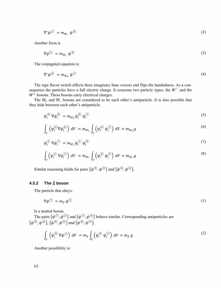
63
Another form is
The conjugated equation is:
The sign flavor switch affects three imaginary base vectors and flips the handedness. As a con-
sequence the particles have a full electric charge. It concerns two particle types, the and the
bosons. These bosons carry electrical charges.
The and bosons are considered to be each other’s antiparticle. It is also possible that
they hide between each other’s antiparticle.
∫ ( )
∫ ( )
∫ ( )
∫ ( )
Similar reasoning holds for pairs { } and { }.
4.5.2 The Z boson
The particle that obeys:
Is a neutral boson.
The pairs { } and { } behave similar. Corresponding antiparticles are
{ }, { } and { }.
∫ ( )
∫ ( )
Another possibility is:
(2)
(3)
(4)
(5)
(6)
(7)
(8)
(1)
(2)
64
The pairs { } and { } behave similar. Corresponding antiparticles are
{ }, { } and { }.
4.6 Resulting particles
Under the resulting particles fall 12 multi-color couplings.
{ } { } { } { } { } { }
{ } { } { } { } { } and { }
With these go 12 antiparticles, which form the same set.
The multi-color couplings are anisotropic QPAD’s that are coupled to other anisotropic
QPAD’s that only differ with respect to their color. They show great resemblance with mesons.
Further, we have XX particles via pairs { } { } and { }. They are -1/3 e
charged bosons and have antiparticles { } { } and { }.
We have Y particles via pairs { } and { }. They are -1/3 e charged bosons and
have antiparticles { } and { }.
We have YY particles via pairs { } { } and { }. They are 1/3 e charged
bosons and have antiparticles { } { } and { }.
Finally, we have ZZ particles via pairs { } and { }. They are -1/3 e charged
bosons and have antiparticles { } and { }.
4.7 Antiparticles
Just like the universe is filled with a huge number of particles, it is also filled with a huge
number of antiparticles. This anti-world has its own kind of background QPAD’s. It represents the
local superposition of the tails of the state functions of a category of antiparticles in universe.
Otherwise the antiparticles would not sense the same kind of inertia that particles do.
4.8 Shadow particles
Several particle types have properties and behavior that are similar to the properties and behav-
ior of antiparticle types of other particle types.
For example { } is hidden behind the positron which is the antiparticle of the electron
{ }. The boson { } hides behind the antiparticle of the boson { }
and vice versa.
(3)
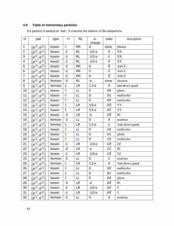
65
4.9 Table of elementary particles
If a particle is marked as ‘anti’, it concerns the shadow of the antiparticle.
nr pair type +/- RL e-
charge
color description
1 { } boson 0 RR 0 none photon
2 { } boson -1 RL -1/3 e XX
3 { } boson -1 RL -1/3 e XX
4 { } boson -1 RL -1/3 e XX
5 { } boson -2 RR 0 Anti Z
6 { } boson -2 RR 0 Anti Z
7 { } boson -2 RR 0 Anti Z
8 { } fermion -3 RL -e none electron
9 { } fermion 1 LR 1.3 e anti-down quark
10 { } boson 0 LL 0 gluon
11 { } boson 0 LL 0 multicolor
12 { } boson 0 LL 0 multicolor
13 { } boson 1 LR 1/3 e YY
14 { } boson 1 LR 1/3 e YY
15 { } boson -3 LR -e
16 { } fermion -2 LL 0 neutrino
17 { } fermion 1 LR 1.3 e Anti-down quark
18 { } boson 0 LL 0 multicolor
19 { } boson 0 LL 0 gluon
20 { } boson 0 LL 0 multicolor
21 { } boson -1 LR -1/3 e ZZ
22 { } boson -3 LR -e
23 { } boson -1 LR -1/3 e ZZ
24 { } fermion -2 LL 0 neutrino
25 { } fermion 1 LR 1.3 e Anti-down quark
26 { } boson 0 LL 0 multicolor
27 { } boson 0 LL 0 multicolor
28 { } boson 0 LL 0 gluon
29 { } boson -3 LR -e
30 { } boson -1 LR -1/3 e Y
31 { } boson -1 LR -1/3 e Y
32 { } fermion -2 LL 0 neutrino
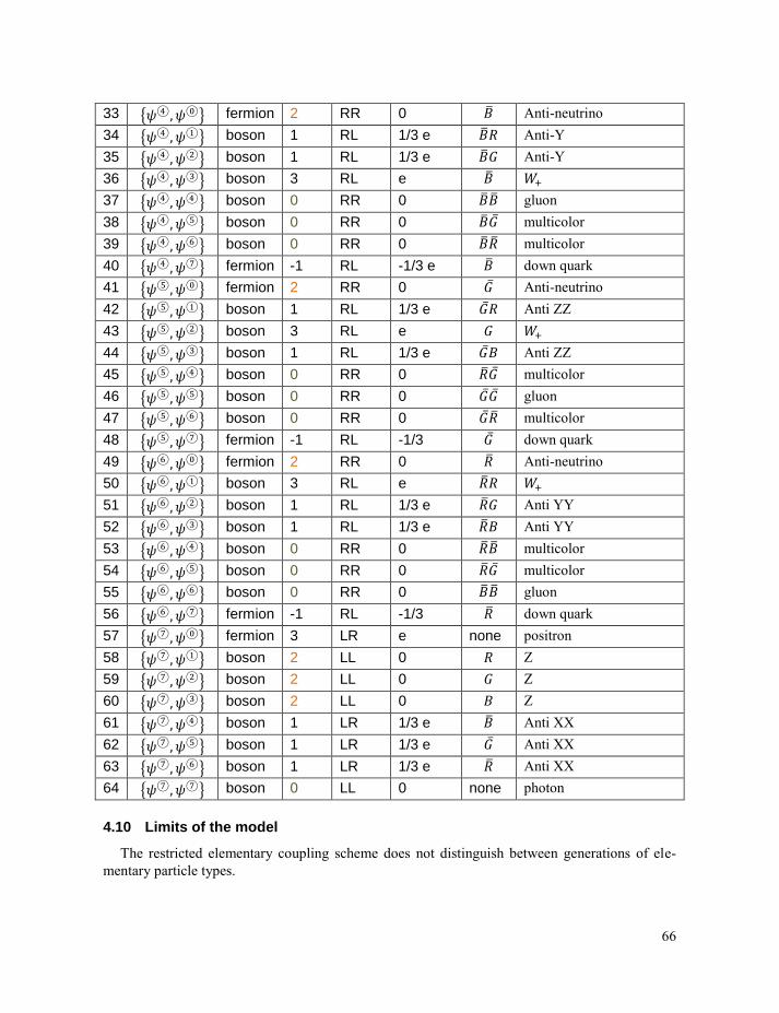
66
33 { } fermion 2 RR 0 Anti-neutrino
34 { } boson 1 RL 1/3 e Anti-Y
35 { } boson 1 RL 1/3 e Anti-Y
36 { } boson 3 RL e
37 { } boson 0 RR 0 gluon
38 { } boson 0 RR 0 multicolor
39 { } boson 0 RR 0 multicolor
40 { } fermion -1 RL -1/3 e down quark
41 { } fermion 2 RR 0 Anti-neutrino
42 { } boson 1 RL 1/3 e Anti ZZ
43 { } boson 3 RL e
44 { } boson 1 RL 1/3 e Anti ZZ
45 { } boson 0 RR 0 multicolor
46 { } boson 0 RR 0 gluon
47 { } boson 0 RR 0 multicolor
48 { } fermion -1 RL -1/3 down quark
49 { } fermion 2 RR 0 Anti-neutrino
50 { } boson 3 RL e
51 { } boson 1 RL 1/3 e Anti YY
52 { } boson 1 RL 1/3 e Anti YY
53 { } boson 0 RR 0 multicolor
54 { } boson 0 RR 0 multicolor
55 { } boson 0 RR 0 gluon
56 { } fermion -1 RL -1/3 down quark
57 { } fermion 3 LR e none positron
58 { } boson 2 LL 0 Z
59 { } boson 2 LL 0 Z
60 { } boson 2 LL 0 Z
61 { } boson 1 LR 1/3 e Anti XX
62 { } boson 1 LR 1/3 e Anti XX
63 { } boson 1 LR 1/3 e Anti XX
64 { } boson 0 LL 0 none photon
4.10 Limits of the model
The restricted elementary coupling scheme does not distinguish between generations of ele-
mentary particle types.
67
It must be stated that the reason of being a fermion as it is applied here, differs strongly from
the usual fermion/boson assignment. As a consequence also the notion of spin will differ. This
approach is due to the fact that the elementary particles are defined as a pair of coupled QPAD’s
and not as a single state function QPAD. Only the ordered pair will define the value of the spin
and the fact that the particle is a fermion.
We adopt the existing convention that fermions go together with half integer valued spin. Here
it will not be explained why that relation exists. With other words, having half integer spin and
being a fermion is related on the one hand to experimental results and on the other hand to the or-
dered pair of coupled QPAD’s that represents the particle. In the HBM according to the current
rules, a particle is a fermion when its state function is coupled to the general background QPAD.
What spin actually is, is not explained in this model. We just accept the existing convention. The
same holds for the electrical charges.
In short, this model does not explain why particles get their electric charge or spin. The model
only explains the origin and the habits of the coupling factor and it explains how the values of the
electric charge and spin relate with the ordered coupled QPAD pair that represents the particle.
Later, it will be explained how the coupling factor relates to the mass of the particle.
The scheme does not provide a way to construct up-quarks from coupled QPAD’s. Their elec-
tric charge conflicts with the existence of anti-neutrinos. Instead the scheme provides some extra
particles that do not appear in the standard model. It might be possible to compose up-quarks from
a combination of XX particles and positrons or compose up-quarks from a combination of XX
particles and particles.
With this addition and by neglecting generations the scheme is capable to generate all known
elementary particles that are contained in the standard model. In fact if generations are neglected,
then the generated set is much larger than the standard model. This is only partly due to the fact
that color charge is considered for all anisotropic particles.
The scheme comprises electrons, positrons, neutrinos, anti-neutrinos, down quarks, anti-down
quarks, particles, particles, Z particles, anti-Z particles, photons and gluons. Where appli-
cable these particles appear with color charge. Color charge is noticeable for down quarks when
baryons of three down quarks are formed.
Extra particles are the multicolor particles, the Y-particles, the XX particles, the YY particles
and the ZZ particles.
68
5 Origin of curvature
The primary QPAD’s cause local pressure differences in the QPAD-sphere. This only occurs
when the QPAD is coupled to another QPAD. For a restricted elementary coupling both QPAD’s
must be sign flavors of the same base QPAD. On its turn the local pressure causes a local space
curvature.
5.1 Physical fields
In the HBM two categories of physical fields exist. The first category is formed by free prima-
ry QPAD’s. These QPAD’s oscillate. Depending on their sign flavor they are photons or gluons.
Primary QPAD’s are linked with an eigenvector of an operator in separable Hilbert space. For the
free primary QPAD’s this is the canonical conjugate of the locator operator.
The second category is formed by fields that represent the properties of the couplings of prima-
ry QPAD’s that correspond to elementary particles. These properties are coupling factor, electric
charge and spin. The state functions of massive elementary particles are primary QPAD’s that are
linked with an eigenvector of the particle locator operator in separable Hilbert space. The corre-
sponding physical fields are gravitation fields, electrostatic fields and magnetostatic fields. These
fields move with the particles, but they do not oscillate like the first category does. However, in
atoms the elementary particles may oscillate.
It is assumed that in atoms only the state function QPAD part of the coupled QPAD pair oscil-
lates and the other part; the background QPAD, stays stable. It implements inertia. Still it moves
with the movement of the atom as a whole. The physical field that represents the influence of a
property of an elementary particle is assumed to be attached to the background QPAD of that el-
ementary particle. Thus this second category physical field does not oscillate. A first category
physical field is released or absorbed when the elementary particle switches its oscillation status.
With other words, photons and gluons are fundamentally different from the second category of
physical fields.
This may be the reason that photons cannot pass the event horizon of black holes, while the in-
formation of the BH’s mass, electric charge and spin are available to the environment of the BH.
5.2 Curvature and inertia
All primary couplings affect the local curvature
Only the state function QPAD’s that couple to a background QPAD will experience inertia
This holds for particles as well as for antiparticles.
5.2.1 Inertia versus antiparticle
Besides of the fact that all particles possess corresponding antiparticles, each state function
category seems to correspond with a corresponding background QPAD, which in some cases is
the conjugate of the state function QPAD. That happens with W particles and leptons. Fermions
69
and their antiparticles seem to prefer isotropic background QPAD’s. Most fermions share the
same (isotropic) background QPAD and anti-fermions do the same.
5.2.2 Inertia of W and Z Bosons
W and Z bosons use their “own” background QPAD, which is anisotropic.
The background QPAD of a boson has the form of the state function QPAD of a boson,
which has the form of an anti- boson.
The background QPAD of a boson has the form of the state function QPAD of a boson,
which has the form of an anti- boson.
5.3 Effect of primary coupling
The coupling may compress or decompress the local parameter space.
In the table above, 56 different kinds of primary coupling are discerned.
Together with the balance equations that differ for particles and antiparticles and shadow parti-
cles this defines a large number of ways of how the local parameter space is affected.
70
5.4 The HBM Palestra reviewed
In the Hilbert Book Model all QPAD’s and the fields that are derived from them or from their
couplings, share the same parameter space. For that reason this common parameter space has been
given a special name; the HBM Palestra56. This shared parameter space spreads universe wide. It
is the place where universe is located.
The parameter space of the QPAD can be interpreted as a quaternionic distribution. It has itself
a parameter space, which is formed by a 3D continuum. This continuum is taken from the eigen-
space of a location operator that resides in the Gelfand triple of the separable Hilbert space. Only
the imaginary part of the quaternionic distribution is used. It can be considered as a 3D Riemanni-
an manifold. The local metric defines the local curvature. What occurs in this manifold is de-
scribed by the QPAD’s.
The Palestra is the playground of all what happens in fundamental physics. It is governed by a
special kind of fluid dynamics57. Things like charge density distributions, current density distribu-
tions, sources, drains, compressed regions and decompressed regions occur in this space58. The
QPAD's are not the transporters. They only describe the transport process. The action takes place
in their shared parameter space. That’s how these QPADS’s can influence each other.
The sources and drains are controlled by Poisson processes59. The generated quanta take a
probable track. The most probable track has preference. Thus the currents described by the
QPAD’s are corridors rather than actual paths. Similarly the locations of the charges in the density
distributions are places where charges may exist with corresponding probability. It need not be the
place where the charges are. The phrase “is governed by a special kind of fluid dynamics” must be
interpreted in this view. The transported quanta are sparsely present in the HBM Palestra.
Nevertheless this special space may be characterized by notions such as temperature and entro-
py. Both indicate a relation with information.
Two kinds of processes determine the dynamics in the parameter space. The first kind is
formed by quantum generating or quantum annihilating Poisson processes. The second kind is
caused by the coupling of QPAD’s. It means that the dynamics in the parameter space can be de-
scribed by a combination of fluid dynamics and statistical mechanics.
Since the HBM implements dynamics via a sequence of pages, each HBM page only shows the
static status quo of the parameter space. The real part of the quaternionic distributions that define
the HBM Palestra can be used to store the progression parameter.
The elementary coupling equation is a continuity equation. It describes primary couplings. The
coupling can be characterized by a small set of properties. These properties are conserved. Most
of these properties can be considered as sources of second category physical fields. These second
category physical fields correspond to physical fields that are attached to the corresponding ele-
mentary particle.
56 The name Palestra is suggested by Henning Dekant’s wive Sarah. It is a name from Greek
antiquity. It is a public place for training or exercise in wrestling or athletics 57 See: Quantum fluid dynamics 58 Vortexes may also appear in the Palestra. The HBM does not yet treat them. 59 See: What image intensifiers reveal

71
The elementary coupling equation appears in 64 forms. Eight of these correspond to a zero
coupling factor, thus these situations describe free QPAD’s. It concerns photons and gluons. The
56 resulting cases concern specific elementary particles. Thus, there are 56 ways to constitute a
primary coupling. This count neglects the antiparticle equation. Thus, a very large number of dif-
ferent primary couplings are possible.
After a coupling the resulting currents need not be exhausted completely. The properties of the
coupling are conserved and the corresponding physical fields and the resulting currents can be ex-
ploited in higher order coupling. So what happens at these scales can become very complicated.
At some distance from the elementary particle the dynamics can be described as incompressi-
ble flow. However, close to the particle, thus close to the coupling the dynamics must be treated
as compressible flow. It means that features like compression, entropy and temperature will start
to play a role.
In short; the HBM Palestra is the sparsely occupied internally moving space that is used as pa-
rameter space by all QPAD’s that play a role in the HBM.
5.5 What image intensifiers reveal
The author spent eighteen years in the development of image intensifier tubes. These devices
range from goggles via driver scopes to fourteen inch wide X-ray image intensifiers.
The image intensifiers had one feature in common. They were all capable of turning the im-
pingement of a quantum at their input screen into a visible light spot at their output screen. A hail
storm of impinging quanta at the input resulted in a noisy film at the output606162.
The starlight scopes enable visibility of very low dose scenes under starlight conditions. They
turned infrared and visible light quanta into light spots on a luminescent phosphor screen.
The X-ray image intensifiers were designed to deliver a perceptible image of an X-ray shadow
picture at the lowest possible X-ray dose for the diagnosed patient.
What still astonishes me is that I never saw any indication of a wave entering the input of the
image intensifiers. I only saw clouds of quanta. That does not say that these clouds cannot have
the shape of waves, but the detected quanta did not show that relation.
With other words, what we can observe are the quanta. We cannot observe the envelop of the
quantum clouds. We cannot observe the waves!
This is a significant experience. Light as a wave does not exist as a physically observable ob-
ject. It only exists as a bunch of quanta. That quantum cloud may have the shape of a wave, but
we cannot discern that wave. We can only detect interferences of these waves because the patterns
of the detected quanta take that shape, but we cannot observe the interferences themselves.
What are then these quanta that impinge on the inputs of our detectors? They are tiny patches
of something.
The Hilbert Book Model makes a very particular assumption about these quanta.
The HBM interprets the quanta as tiny patches of the parameter space of the state function.
Further the HBM uses state functions that are quaternionic probability amplitude distributions.
This makes it possible to interpret the state functions as combinations of charge density distribu-
60 See: http://en.wikipedia.org/wiki/File:Moon_in_x-rays.gif . Low dose X-ray image of the moon. 61 See: http://www.youtube.com/watch?v=U7qZd2dG8uI ; Hail storm. Warning, this is NOT a vid-
eo of an external object. 62 Also see: http://en.wikipedia.org/wiki/Shot_noise
72
tions and current density distributions. The state functions may also contain sources, drains, com-
pressed regions and decompressed regions. These features all occur in the parameter space of the
state function.
This daring interpretation explains why in the neighborhood of particles the parameter space
appears to be compressed.
When measuring the properties of image intensifiers it appeared that the distribution of detect-
ed quanta can be characterized as a Poisson distribution. That indicated that the generators of the
quanta can be considered as Poisson processes. It is well known that Poisson processes that are at-
tenuated by subsequent binomial processes can be treated as a new less efficient Poisson process.
Spatial and temporal spread can be interpreted as a binomial processes. It is also known that very
efficient Poisson processes produce distributions that are close to Gaussian distributions. When
looked upon as a charge distribution the Gaussian distribution produces a potential that approach-
es an Error function. At some distance from the generator the Error function takes the form of a
1/r function. On its turn this corresponds with a single charge source. Thus from a distance the
generator looks as a (singular) single charge source. Of course the actual generator is not singular!
This gives a particular insight in radiation sources!
5.6 Quantum Fluid Dynamics
What happens in the HBM Palestra is controlled by Quantum Fluid Dynamics (QFD). QFD
differs from conventional fluid dynamics in that in QFD the charge density distributions and cur-
rent density distributions describe probable locations and paths in their own parameter space,
while in conventional fluid dynamics these distributions describe actual locations and paths that
occur in a considered medium such as a gas or liquid. That is why in QFD the charge density dis-
tributions and current density distributions are combined in quaternionic probability amplitude
distributions, while in conventional fluid dynamics they are located in scalar and vector fields.
These fields can also be combined in quaternionic distributions, but they are not probability am-
plitude distributions.
Already in 1927 Erwin Madelung63 published a set of equations that treat quantum physics in
the sense of QFD.
63 See: http://en.wikipedia.org/wiki/Madelung_equations
73
6 Higher level coupling
The primary QPAD’s cause a local pressure in the QPAD-sphere. On its turn that local pres-
sure causes the local space curvature.
The streams of space patches that result after the primary couplings will be used in higher level
interactions. It means that these resulting currents may still influence higher level coupling.
Hypothesis:
In these interactions the properties of the primary couplings are conserved
6.1 A quaternionic theory of general relativity
A special quaternion based equivalent of general relativity theory (GRT) applied to the shared
parameter space of QPAD’s Palestra can be put together. Some of the ingredients for that theory
are present in the appendix chapters 13 and 14. A quaternionic version of GRT will offer similar
results as conventional GRT does. In the HBM this is not worked out in detail because the quater-
nionic GRT only gives information on curvature and does not give detailed information on how
higher level coupling works.
6.2 The Kerr-Newman equation
The Kerr-Newman equation is NOT part of the HBM. The Kerr-Newman equation is a solution
of conventional General Relativity Theory. It uses spherical coordinates as a reference frame. The
Kerr-Newman equation describes the effects of physical fields on curvature for elementary parti-
cles as well as for black holes
The Kerr-Newman metric equation gives only a rough impression on how the primary cou-
plings influence curvature. This equation uses parameters that are comparable to the properties of
primary couplings. The equation neglects the geometry of these couplings and the resulting flow
of space patches. For that reason it can only deliver a coarse approximation. For that reason the
HBM only uses the Kerr-Newman equation in order to get a coarse idea of how GRT curvature
relates to the curvature that is caused by elementary couplings.
6.3 Role of second category physical fields
The properties that characterize primary couplings act as sources/drains of second category
physical fields
The primary couplings are responsible for affecting the local curvature, but it looks as if the se-
cond category physical fields have this role
This is a false impression!
6.4 Higgs
This story does not include a Higgs particle or a Higgs field. However, the Hilbert Book model
uses a background field that acts as a partner in the coupling of that background field to the state
74
function of an elementary fermion. That background field takes the role of the Higgs field. It im-
plements inertia. This simplified picture ignores that every coupled QPAD in some way affects
curvature. The coupling not only explains the existence of curvature, it also explains the existence
of inertia.
75
7 HADRONS
The HBM cannot discern generations of elementary particles. For that reason the elementary
fermions are treated per category.
Symbol e or means electron
Symbol p or means positron
Symbol n means neutrino
Symbol d means down-quark
Symbol u means up-quark. But in the HBM up-quarks are no elementary particles.
7.1 Second level coupling
This chapter treats the second level of coupling. It treats couplings between elementary parti-
cles. This coupling uses the second category physical fields that are generated by the properties of
the first level coupling. The Hilbert Book Model delivers the reason of existence of these proper-
ties; coupling factor, electric charge, angular momentum (spin) and possibly color charge of ele-
mentary particles. In higher level couplings these properties are conserved. Higher level coupling
might also use what is left of primary QPAD’s after primary coupling.
The primary couplings influence the local curvature. However, the primary QPAD’s are not
observable. Only the second category physical fields become observable. Thus, it looks as if the
second category physical fields or their sources/drains are responsible for affecting curvature.
This, of course, is a false impression.
The currents in the coupled primary QPAD’s that remain after coupling may still influence
higher level coupling.
The curvature is also a binding ingredient for the next levels of coupling. The formulas that de-
scribe the influence of the conserved properties on the curvature inform what will happen. Cur-
rently the best available formula is the Kerr-Newman metric formula, which is taken from GRT.
The Kerr-Newman equation works on the base of locally existent properties (the sources or drains
of the second category physical fields). It must be reckoned that the Kerr-newman equation gives
only a rough indication of what happens. In order to know what happens in detail the full Quan-
tum Fluid Dynamic situation must be analyzed.
At a fixed instant of proper time, thus inside a single page of the Hilbert Book Model, the Kerr-
Newman equation is a static equation.
If in a subsequent HBM page the controlling properties have changed, then those new proper-
ties define the new configuration.
The first level coupling that constitutes elementary fermions uses a background field that is the
partner in the coupling of that background field to the state function of the elementary fermion.
The background field represents the superposition of the tails of the state functions of all mas-
sive particles that exist in the universe. In this way inertia gets its implementation.
If particles couple, then their background QPAD’s will superpose. Thus their inertia will com-
bine.
76
Hadrons are the first of the next levels of binding products.
The Kerr-Newman equation shows an abnormality at the place where black holes get their
horizon. Whether or not a hadron possesses a horizon is in this respect unimportant. The proper-
ties of the elementary particles that are bound together in order to form the hadron are sources of
second category physical fields. The static versions of these second category physical fields reach
beyond a possible horizon. To the outside world the superposition of these fields signal the prop-
erties of the hadron.
The primary QPAD’s that constitute the elementary particles and that on their turn constitute
the hadron also reach beyond the potential horizon.
7.2 Interaction
The conventional way of treating interactions in quantum field theory is to apply a methodolo-
gy called covariant derivation. This methodology works well in a complex representation, but
fails in a quaternionic approach. With other words it works in special one-dimensional cases but it
is not well suited for multidimensional cases. So, the HBM must find another approach in order to
implement interactions. The HBM also does not consider the existence of virtual particles. How-
ever, this is compensated by the availability of primary QPAD’s. These primary QPAD’s describe
the probability of presence of virtual carriers of charges, where the charges can be ensembles of
properties of that carrier. Superpositions of tails of these QPAD’s can construct temporary cou-
plings. These couplings will in fact represent temporary virtual particles. This deliberation leads
to the acceptance of the superposition of the tails of QPAD’s as the medium that implements the
feature of interaction.
7.3 Rules
The second level of coupling has its own set of rules.
The total color of the composite must be white64.
The properties of the constituting particles will be conserved.
However, mass (coupling factor) may be exchanged against field energy.
Field energy is transported via oscillating QPAD’s.
Like the fermions, hadrons exist in generations.
The properties of the elementary particles, including color, play a significant role in the Pauli
principle. (The HBM does not explain the Pauli principle).
Coupling factor, electric charge, angular momentum (spin) and may be color charge are
sources of second category physical fields.
Location (position or momentum) are not sources of second category physical fields.
64 In observable particles, which are particles that may be detected in measuring machines like
the LHC, the color is always white.
77
7.4 Up-quarks
In the HBM the up-quarks cannot be constructed from a primary coupling of QPAD sign fla-
vors. Therefore the HBM does not consider them to be elementary particles. Instead up-quarks are
composed of down-quarks or XX particles and W+ particles or from down-quarks or XX parti-
cles, positrons and neutrinos. May be YY particles or ZZ particles are also involved. Further, the
up-quarks annihilate into these constituents.
Like down-quarks the up-quarks have color. This attribute relates to the direction of the reflec-
tion of the constituting down-quark.
Apart from up-quarks also anti-up-quarks exist.
7.5 Mesons
Mesons are composed out of quarks and anti-quarks. The following meson categories exist.
(dd+uu)/√2
(dd-uu)/√2
ud
du
However, it might well be that the mixed color elementary particles are in fact mesons.
7.6 Baryons
Baryons are composed out of triples of quarks. The following baryons exist65.
Symbol configuration name Isospin I3
ddd delta ⁄
ddu neutron ⁄
uud proton ⁄
uuu delta ⁄
For the anti-baryons the possibilities are:
ddd
ddu
uud
uuu
I relation to the Pauli principle the versions with multiple u or multiple d can only exist due to the
fact that the constituting quarks have different spin and/or different color charge.
t
65 The generations are ignored!
78
8 THE BUILDING
The building consists of everything that can be assembled from elementary particles, hadrons
and fields.
8.1 Natures Music
In atoms electrons oscillate around a central point that acts as the location of the atom66. In
molecules the same features occur in an even more complicated configuration.
The oscillations are harmonic. The most basic harmonic oscillations are, apart from a scalar
factor, invariant under Fourier transformation67. These oscillations have modes and usually sever-
al of these modes exist in parallel. These modes can be generated and annihilated. Generation
goes together with the absorption of a more elementary particle or elementary wave and annihila-
tion goes together with a corresponding emission.
8.2 Hydrogen atom
In the hydrogen atom68 one electron encircles the nucleus. The oscillation of the electron can
be described as a quantum spherical harmonic oscillation. It can have different oscillation modes.
These modes are characterized by quantum numbers. Mode switching is activated by creation and
annihilation operators. The speed of the electrons is high enough such that relativity effects must
be considered. Also the spin of the electron plays a role and causes magnetic effects.
8.3 Helium atom
In the helium atom69 two electrons encircle the nucleus. In principle the electrons behave simi-
larly as in the hydrogen atom, however due to the Pauli principle they cannot both occupy the
same oscillation mode. The electrons not only interact with the nucleus, but they also interact with
each other.
8.4 Modularization
Hadrons, atoms and molecules are products of a modularization process.
Modularization70 encapsulates properties in a higher order individual and renders the resulting
individual a specific behavior. Its main purpose is that the number of relations to the outside
world is reduced. Usually the module can be accessed via a series of well-defined interfaces. The
whole keeps the integrity of the individual intact.
Modularized systems are far simpler than their monolithic equivalents. Modularization exploits
reuse. The modularization can have far reaching consequences. That is especially the case when
modules can be used to create a new kind of modules. In this way nature is capable of construct-
66 Appendix; Oscillations 67 Appendix; Functions invariant under Fourier transformation. 68 http://en.wikipedia.org/wiki/Hydrogen_atom 69 http://en.wikipedia.org/wiki/Helium_atom 70 http://vixra.org/abs/1101.0064
79
ing very complicated systems. On earth nature achieved the stage to be able to generate intelligent
species. This tendency goes straightly against the tendency that is set by the second law of ther-
modynamics. These laws prescribe that disorganization, randomness and chaos will increase con-
tinuously.
8.5 Black hole
8.5.1 Classical black hole
According to classical mechanics the no-hair theorem71 states that, once a black hole achieves a
stable condition after formation, it has only three independent physical properties:
mass,
charge, and
angular momentum.
The surface gravity72 may be calculated directly from Newton's Law of Gravitation73, which
gives the formula
m
r
where m is the mass of the object, r is its radius, and is the gravitational constant74. If we let
denote the mean density of the object, we can also write this as
r
For fixed mean density , the surface gravity is proportional to the radius .
Sciama75 relates to the potential that is raised by the community of particles. For fixed mean
density this is shown by
∫
∫
Here is the current radius of the universe.
71 http://en.wikipedia.org/wiki/No-hair_theorem 72 http://en.wikipedia.org/wiki/Surface_gravity 73 http://en.wikipedia.org/wiki/Newton%27s_Law_of_Gravitation 74 http://en.wikipedia.org/wiki/Gravitational_constant 75 Influence;Inertia
(2)
(3)
(4)
(5)
80
8.5.2 Simple black hole
The Schwarzschild radius for a non-rotating spherical black hole is
8.5.3 General black hole
More generally holds
where
is the mass/energy,
is the horizon area,
is the angular velocity,
is the angular momentum,
is the electrostatic potential,
is the surface gravity,
is the electric charge.
For a stationary black hole, the horizon has constant surface gravity.
It is not possible to form a black hole with surface gravity. .
8.5.4 Quantum black hole
When quantum mechanical effects are taken into account, one finds that black holes emit ther-
mal radiation (Hawking radiation) at temperature
A quantum black hole is characterized by an entropy and an area .
The entropy of a black hole is given by the equation:
The Bekenstein-Hawking Entropy of three-dimensional black holes exactly saturates the bound
where is the two-dimensional area of the black hole's event horizon in units of the Planck
area,
(1)
(1)
(1)
(2)
(3)
81
.
In the Hilbert book model this equals the number of granules that covers the horizon of the
black hole.
The horizon of the black hole is an event horizon because information cannot pass this horizon.
(Near the horizon the speed of light goes to zero.)
8.5.5 Holographic principle
The holographic principle76 states that the entropy contained in a closed surface in space equals
the entropy of a black hole that has absorbed everything that is contained in this enclosure.
In the Hilbert book model it means that if the surface is considered as a sparsely covered hori-
zon, then that sparse horizon contains as many granules as the densely covered horizon of the cor-
responding black hole.
It also means that the maximum entropy that can be contained inside a surface corresponds to a
dense coverage with granules of that surface.
In this model, any dense or sparse horizon reflects via its contained entropy the number of
granules that are contained in the corresponding volume.
We might extend this picture by stating that the number of granules in a volume corresponds
with the entropy in the volume. In the Hilbert book model the number of granules corresponds to
the number of Hilbert vectors that are attached to a QPAD. It also corresponds to the number of
anchor points of the primary physical fields.
The eigenvectors of the particle locator operator 𝔖 correspond to quantum logical propositions
that represent the location of physical particles. These propositions have a binary yes/no value. In
the extended model these propositions get extra content via the attached QPAD’s.
8.5.6 Black hole as a subspace of the Hilbert space
The coupling between the eigenvectors of the particle locator operator and the Palestra is not
precise. It is stochastic and its minimal size is of the order of the Planck-length. This granularity is
due to the fact that the Hilbert space is separable and as a consequence the set of eigenvalues is
countable. That is why the granules in the surface of a black hole have this size. The surface of a
black hole is an image of the unit sphere of a subspace of the Hilbert space where the eigenvectors
of the particle location operator form an orthogonal base and all attached QPAD’s pack the eigen-
values together in an optimal way.
The eigenvectors of the particle locator operator all touch such a granule. The relation with
quantum logic means that the Hilbert vector stands for a proposition that has a yes/no value. In
case of the Hilbert vectors that are attached to the granules the yes/no value represents group
membership. Thus each granule represents a bit of information.
For the eigenvectors of the particle locator operator a densest packaging exists. It means that in
that condition the QPAD’s have shrunk to their smallest possible location difference.
76 http://en.wikipedia.org/wiki/Holographic_principle
(4)
82
Assumption 1: In that condition, due to the properties of the QPAD’s, the mutual tension
works asymmetrically.
This asymmetry means that in a surface that is formed by a set of densely packed granules the
tension on one side is stronger than the surface tension at the other side. As a consequence the fi-
nal configuration of a densest packaging becomes an empty bubble.
8.5.7 HBM interpretation of black hole
Three dimensional granular structures do not occur in nature other than in composites that have
a regular structure. A regular granular structure of space would immediately cause anisotropy of
that space. Still space includes two dimensional regular granular structures. They form the surfac-
es of black holes. They also represent the most densely form of packaging of entropy.
The surface patches can be seen as to represent Hilbert eigenvectors of the particle location op-
erator. For these eigenvectors the corresponding eigenvalues are packed densely together into a
surface. The packed eigenvectors all carry the properties of their mutual coupling. (mass, electric
charge, spin). Together these data form the properties of the BH.
The coupling of the QPAD’s that are attached to the packed eigenvectors is a special type that
is not treated before. Its characteristics are such that the coupled particles form a stable bubble
shaped body. This body can still absorb extra particles.
Black holes feature seemingly contradictory properties. On the one hand information cannot
pass their event horizon. On the other hand it is possible to follow their history from occurrences
in their environment. This history follows from the values of their properties. These properties are
represented by second category physical fields. Thus the second category physical fields CAN
pass event horizons, while first category physical fields are blocked. This indicates that the two
categories are fundamentally different.
8.5.8 Chandrasekhar limit
The Chandrasekhar limit77 is an upper bound on the mass of a stable white dwarf star:
√
(
)
⁄
where:
is the reduced Planck constant
c is the speed of light
G is the gravitational constant
μe is the average molecular weight per electron, which depends upon the chemi-
cal composition of the star.
77 http://en.wikipedia.org/wiki/Chandrasekhar_limit
(1)
83
mH is the mass of the hydrogen atom.
. is a constant connected with the solution to the Lane-Emden
equation.
Approximately:
.
Where
√ c ⁄ is the Planck mass
8.5.9 Similarity between black hole and massive fermion
According to the no hair theorem a black hole shows only a few properties to the outside
world. These properties are sources of second category physical fields.
Massive fermions have a similar behavior.
Apart from the exposed features it is impossible to observe what goes on inside the black hole.
It is possible that the internals of a black hole are to a certain extent similar to the construction
of a massive fermion. It would mean that the BH is based on a set of QPAD’s that each are cou-
pled to a background QPAD.
8.6 Birth of the universe
For the eigenvectors of the particle locator operator a densest packaging exists. It means that in
that condition the QPAD’s have shrunk to their smallest possible location difference.
Assumption 1: In that condition, due to the properties of the QPAD’s, the mutual tension
works asymmetrically.
This asymmetry means that in a surface that is formed by a set of densely packed granules the
tension on one side is stronger than the surface tension at the other side. As a consequence the fi-
nal configuration of a densest packaging becomes an empty bubble.
In the starting condition of the universe all eigenvectors of the particle locator operator are
densely packed in one assembly.
Assumption 2: At an instant after that moment the packaging density suddenly relaxes.
Even when the chance is very low, which means that the start bubble is very stable, given
enough time the occasion will certainly happen. (It means that black holes may collapse.)
The number of granules does not change. Thus, during this spreading the total entropy does not
change.
(2)
(3)
84
The package may fall apart in several separated subassemblies and a large series of single or
more loosely packed granules. For the single and the more loosely packed granules the corre-
sponding QPAD’s fold out. The densely packed subassemblies take again a bubble shape.
This process may occur instantly or gradually, but most probably it will be done in a sequence
of these two possibilities.
First occurs a sudden change of scale between the particle locator operator in the separable
Hilbert space Ң and the GPS operator that delivers the background coordinate system and that re-
sides in the rigged Hilbert space Ħ. It is possible that originally the bubble covered the whole of
the unit sphere of the Hilbert space Ң, or it may just cover a finite dimensional subspace of Ң.
This means that the bubble contains an infinite or a finite amount of granules, which suddenly get
diffused in a much larger space. That space is affine like the unit sphere of the Hilbert space Ң.
The diffusion takes place at every occupied location in the background coordinate system.
This kind of universe has no spatial origin or it must be the center of the outer horizon. With
the aid of the background coordinate system, it will be possible to indicate a center of that uni-
verse. Each item in this universe has its own private information horizon. This horizon is set by
the reach of the light that has been travelling since the birth of the universe. As long as this light
does not reach the outer horizon that sub-universe looks isotropic. A multitude of such sub-
universes exist that need not overlap. However, they all look at their border at an image of part of
the start horizon. Such, sub-universes obey the cosmological principle78.
In the next phase the further expansion occurs gradually. Because the QPAD’s that are attached
to the granules install a tendency for the granules to stay together, a different motor must be pre-
sent behind this expansion. This motor can be found in the fact that with increasing radius the
number of pulling granules grows faster than the decrease of the forces that are executed by the
fields of these granules that is caused by the increasing distance. In an affine space this is always
and everywhere true. This effect is also the source of inertia.
Due to local attraction, loosely packed and single granules may reassemble in bubble shaped
subassemblies. These subassemblies are known as black holes. Single granules and small aggre-
gates of granules are known as elementary particles, nuclei or atoms.
Much larger aggregates may be formed as well but these are not densely packed. Elementary
particles can be categorized according to the configuration of their constituting QPAD’s. The
coupled QPAD’s determine how massive the particle is.
Inside the bubble the fact that the granule represents matter is not recognizable. It is only rec-
ognizable when the attached QPAD gets the chance to unfold. That condition is true when the
granule is not part of a densely packed subassembly.
The requirements for the birth of the universe are:
1. The existence of a particle locator operator
78 http://en.wikipedia.org/wiki/Cosmological_principle
85
2. The existence of QPAD’s that install the tendency to keep these eigenvectors of
the particle locator operator together
3. When the large numbers of eigenvectors are densely packed, then the assembly
forms a bubble, because due to the properties of the QPAD’s, the mutual tension
works asymmetrically
4. In advance the eigenvectors of the particle locator operator are densely packed
in one bubble.
5. A non-zero probability exists that the package density will be relaxed and the
package falls apart. This may happen in a two stage process
a. A sudden reduction of scale occurs
b. Next a force that pulls the granules further away from each other exists
In the first episode of the universe the sudden scale change took place. This ripped the original
bubble apart. Next a gradual further expansion took place.
The granules that move freely can at the utmost take one space step at every progression step.
When the ratio of the space step and the progression step is fixed, then this determines a maxi-
mum speed of granules. A certain type of granules takes a space step at every progression step.
That type transports information at the maximum possible speed.
When the path of these information transmitting particles is a straight line, then after a while,
the other types of granules no longer get messages from the birth episode of the universe. But this
need not be the case.
Since the messenger has a finite speed, it brings information from the past. First of all the
speedy messenger and the slow addressee may have started from different locations. Further, due
to curvature of space the path of the speedy messenger may take much longer than the duration of
the much straighter path that the much slower addressee has taken. The information about the past
that is included in the message might be close to the episode in which the granules were combined
in one large bubble.
Thus despite the fact that most of the information that is generated during the birth of the uni-
verse is long gone, still some of that information may reach particles long after the instance of
birth. When this information is interpreted it gives the impression of a metric expansion of the
universe79.
79 http://en.wikipedia.org/wiki/Metric_expansion_of_space

86
87
9 COSMOLOGY
Cosmology concerns all particles with a mass above the limiting mass 𝔐.
9.1 Higher order couplings
It is assumed that during higher order couplings the constituting elementary particles keep their
basic properties;
coupling factor,
electric charge
angular momentum
color charge.
The properties that characterize the coupling event in elementary particles are sources of se-
cond category physical fields. These fields are known as physical fields. For example the electric
charge is a source for electromagnetic fields. The coupling factor is a source for the gravitation
field. The spin also causes a field.
A secondary field is a specialized QPAD that has one of the properties of the elementary parti-
cle as its isolated source. The second category physical fields may still overlap (superpose).
These second category physical fields play a major role in the higher order couplings. The rea-
son for this fact is that the sources of the second category physical fields influence the curvature
of the parameter space. In fact this is a misconception, because the real cause of curvature is
formed by the primary couplings.
In this respect a more complicated effect also plays a role. The currents of the primary QPAD’s
that result after the primary coupling may also influence the higher order coupling. This effect is
not covered by formulas like the Kerr-Newman metric formula.
The composite particles can be considered to have state functions that are formed by the super-
position of the state functions of the constituting particles. However, at least part of these particles
consist of coupled pairs of QPAD’s in which one is a state function QPAD and the other is a
background QPAD. With other words, a composite particle is a coupling between a superposition
of a number of state function QPAD’s and a superposition of a number of background QPAD’s.
Not only the charge density distributions superpose, but also the current density distributions su-
perpose. Thus the flows intermix.
It means that the state function of the composite is a superposition of a set of QPAD’s that
have different sign flavors. However, the same holds for the superposition of the background
QPAD’s.
This fact would mean that higher order coupling is not well described by simple wave equa-
tions as those that describe elementary particles. Instead it may be better described by an equation
that describes the dependence of the local curvature on the locally existing coupling properties.
88
The Kerr-Newman equation produces an abnormality when the limit80
√
is passed. Above that limit the particle is encapsulated and guarded by a skin in the form of a
horizon. Below that limit the enclosed particles are naked.
9.2 Curvature
9.2.1 Hilbert Book Model ingredients
Each page of the Hilbert Book Model consists of three quite independent ingredients.
Ingredient 1: The quantum logic, or equivalently, its lattice isomorphic companion;
the set of closed subspaces of an infinite dimensional separable Hilbert space
Ingredient 2: A background coordinate system, called Palestra that is taken from the
continuum eigenspace of an operator that resides in the Gelfand triple of the separable
Hilbert space.
Ingredient 3: A set of QPAD’s that each couple an eigenvector of a particle locator
operator that resides in the Hilbert space to a value in the Palestra.
Couplings between QPAD’s that lead to elementary particles are characterized by four catego-
ries of properties:
Coupling factor
Electric charge
Angular momentum
Color charge
These primary couplings influence the curvature in the second ingredient that affects the third
ingredient. It looks as if physical fields in the form of second category physical fields that relate to
the primary couplings influence the curvature. This is a misconception. However, this view can
deliver a coarse indication of what happens. The way that these properties influence curvature is
described by metric equations, such as the Kerr-Newman metric formula.
The first category physical fields are restricted by the maximum speed at which information
can be transported. The influence of primary couplings on curvature seems not to be restricted by
this limit. Second category physical fields are not restricted by the maximum speed at which in-
formation can be transported
For example the properties (mass, electric charge, spin and surface area) of a black hole change
in an observable way when matter is absorbed while in the neighborhood of the event horizon the
transport speed of information by first category physical fields is known to reduce to zero.
80 Appendix; Kerr-Newton limit
89
9.2.2 Coordinate system
The coordinate system that is taken from the eigenspace of an operator that resides in the Gel-
fand triple is not applied directly. Instead a quaternionic distribution that uses the values of the flat
coordinate system that is taken from the Gelfand triple as its parameters is used as the observed
coordinate system.
Curvature can be described by the combination of a preselected coordinate system that defines
location in a non-curved space and a local metric that describes the curvature in terms of that co-
ordinate system. As is described above, both the flat and the curved coordinate system are based
on eigenspaces of corresponding operators that reside in the Gelfand triple.
Several coordinate systems are possible. The most common coordinate systems for a non-
curved three dimensional space are:
Cartesian coordinates
Spherical coordinates
Alternatives for spherical coordinates are:
Schwarzschild coordinates81
Kruskal-Szekeres coordinates82
Lemaitre coordinates83
Eddington–Finkelstein coordinates84
The advantage of the alternative coordinates is that they avoid unnecessary singularities. How-
ever, these alternatives are only relevant for situations in which the Schwarzschild radius plays a
significant role. This is certainly the case for black holes and their environment, but it becomes ir-
relevant in the realm of some elementary particles.
9.2.3 Metric
The currently best suitable local metric equation for our purposes is the Kerr-Newman metric85.
It uses three local properties. These properties are:
The coupling factor
The electric charge
The angular momentum
The angular momentum includes the spin .
81 http://en.wikipedia.org/wiki/Schwarzschild_coordinates 82 http://en.wikipedia.org/wiki/Kruskal-Szekeres_coordinates 83 http://en.wikipedia.org/wiki/Lemaitre_coordinates 84 http://en.wikipedia.org/wiki/Eddington%E2%80%93Finkelstein_coordinates 85 Appendix;Metric tensor field;Local metric equation
90
As stated before the Kerr-Newman can only give a coarse approximation because in fact the
primary couplings determine the local situation and the properties represent only abstractions of
these primary couplings.
This Kerr-Newman metric uses the sum of a category of properties that are collected within the
observed sphere. However, in principle the summation produces different centers of activity for
different property categories. Thus, these centers need not be at the same location. However, for
large enough selected radius and applied to black holes or single particles, these centers coin-
cide.
The simplest interpretation of the Kerr-Newman metric can be taken on the surface of a sphere
that has a selected radius .
The formula uses three characteristic radii. The largest characteristic radius plays the most
prominent role.
This fact introduces the notion of geo-cavity.
9.2.4 Scales
The charge-to-mass ratio is typically larger in smaller systems86. For most astrophysical
systems,
,
while for a Millikan oil drop,
.
Going all the way down to elementary particles, the value for the electron is
.
To achieve balance we require that Newton's gravitational force has the same magnitude as
Coulomb's force , that is
| | | |
To be more specific, let us assume that where is the elementary charge. We then ad-
just the mass to the value for which the forces are balanced. This gives the Stoney mass87
√ . g
86 For deeper investigation, see: http://arxiv.org/abs/0802.2914 87 http://en.wikipedia.org/wiki/Natural_units
(1)
(2)
(3)
(4)
(5)
91
It is only one order of magnitude lower than the Planck mass
√ c ⁄ .
g
The ratio between them is given by the square root of the fine structure constant,
α e
c .
√ .
Thus, in case of electric charges, the Coulomb forces are nearly in balance with the gravita-
tional forces at the Planck scale. However, at subatomic scale this picture is disturbed by the spin.
For subatomic systems there is an additional phenomenon which comes into play. In fact, ac-
cording to general relativity, the gravitational field tends to become dominated by the spin at dis-
tances of the order of the Compton wavelength. The relevant quantity which governs this behavior
is the ratio where is the (spin) angular momentum. For an electron,
.
As a consequence, the gravitational field becomes dominated by gravitomagnetic effects in the
subatomic domain. This fact has important consequences for the electromagnetic fields of spin-
ning charged particles.
The four known gravitational and electromagnetic multi-pole moments of the electron are:
the mass ,
the spin ,
the charge
the magnetic moment
The spin is a gravitomagnetic dipole moment, i.e. a gravitational analogue of the magnetic di-
pole moment.
The corresponding Kerr-Newman field is therefore dominated by the spin in the subatomic
domain. In particular, it has no event horizon and it has no ergo-region. (The ergo-region is a re-
gion of space-time located outside the event horizon of a rotating black hole where no object even
if traveling at the speed of light, can remain stationary.)
(6)
(7)
(8)
(9)
(10)
92
An important conclusion is that gravity tends to become spin dominated in the subatomic do-
main.
The Kerr-Newman metric formula indicates that small particles that are encapsulated by a
horizon are restricted by the limit:
√
Where m is the particle mass, is the elementary charge and is the elementary spin.
9.3 Inside black holes
Objects that fulfill the rules for the existence of a BH horizon hide their internals. Their virtual
construction is similar to that of a massive elementary particle. That means that nothing is inside
that horizon than a set of coupled QPAD’s. One of these is a background QPAD. The others form
a superposition. This superposition is a kind of super QPAD. It lets the BH act as one particle that
has the properties of the combination of the gathered fields.
9.4 Hadrons
The Hilbert Book Model delivers the reason of existence of the properties; coupling factor,
electric charge and angular momentum (spin) of elementary particles. In higher level couplings
these properties are conserved. These properties influence the local curvature. The curvature is the
binding ingredient for this next level. The formulas that describe the influence of the conserved
properties on the curvature control what is happening. Currently the best available formula is the
Kerr-Newman metric formula.
This story does not include a Higgs particle or Higgs fields. However, the Hilbert Book model
uses a background field that is one partner in the coupling of that background field to the state
function of an elementary fermion. The background field represents the superposition of the tails
of the state functions of all massive particles that exist in the universe. In this way inertia gets its
implementation. The coupling event is characterized by a set of properties. These are the men-
tioned properties of the elementary particles.
Hadrons are the first of the next levels of binding products.
The Kerr-Newman equation shows an abnormality at the place where black holes get their
horizon. Whether or not a hadron possesses a horizon is in this respect unimportant. The proper-
ties of the elementary particles that are bound together are sources of second category physical
fields. These fields reach beyond a possible horizon. To the outside world the superposition of
these fields signal the properties of the hadron.
(11)
93
10 CONCLUSION
It is quite possible to build a model of physics on a solid axiomatic foundation. It has the ad-
vantage that from the beginning the model stays consistent and trustworthy. For the Hilbert Book
Model this inroad has brought some rather revolutionary deviations from contemporary physics.
The way that fields are treated and how dynamics is implemented differs strongly from the ordi-
nary course of physics. Through the switch from complex Hilbert spaces to quaternionic Hilbert
spaces and the attention that is given to sign flavors of quaternionic probability amplitude distri-
butions it becomes possible to derive unique continuity equations rather than equations of motion.
The elementary coupling equations reveal the properties and habits of all known elementary parti-
cles.
This step only reaches to the first level of binding. The properties of the coupling that occurs
inside elementary particles form the factors that influence the local curvature. The current status
of the model already indicates that the next level of particle binding will use the effects of the
coupling properties on the curvature of the local geometry besides the coupling of sign flavors of
quaternionic probability amplitude distributions. It means that in the higher level binding for a
coarse view the role of the metric equation will be greater than the role of the wave equation. This
step is rather deterministic, while the first level of coupling is afflicted with indeterminism.
94
PART III Appendix
The appendix is a toolbox and a grab bag that contains everything that the author has collected
that can be used to build or analyze the Hilbert Book Model
95
1 Logic
1.1 History of quantum logic
Around 1930 John von Neumann and Garrett Birkhoff were searching for an acceptable expla-
nation of the results of experiments that showed that the execution of an observation of a very
small object can completely destroy the validity of an earlier observation of another observable of
that object. The Schrödinger equation that agreed with the dynamic behaviour of the particles al-
ready existed. Not much later Heisenberg’s matrix formulation became popular as well. Quite
soon the conclusion was made that something was fundamentally wrong with the logic behind the
behaviour of small particles. These small objects show particle behaviour as well as wave behav-
iour and they show quantization effects. It was found that the distribution axiom of classical logic
had to be changed. Soon it became apparent that the lattice structure of classical logic must be
weakened from an ortho-complementary modular form to an ortho-complementary weakly modu-
lar lattice. The quantum logic was born. The next step was to find a useful mathematical presenta-
tion of this new logic. A historic review of what happened can be found in: “Quantum Theory:
von Neumann” vs. Dirac; http://www.illc.uva.nl/~seop/entries/qt-nvd/. It includes extensions of
the concept of Hilbert space and application of these concepts to quantum field theory. Another
source is: http://www.quantonics.com/Foulis_On_Quantum_Logic.html.
1.2 Quantum logic
Elementary particles behave non-classical. They can present themselves either as a particle or
as a wave. A measurement of the particle properties of the object destroys the information that
was obtained from an earlier measurement of the wave properties of that object.
With elementary particles it becomes clear that that nature obeys a different logic than our old
trusted classical logic. The difference resides in the modularity axiom. That axiom is weakened.
The classical logic is congruent to an orthocomplemented modular lattice. The quantum logic is
congruent to an orthocomplemented weakly modulare lattice. Another name for that lattice is or-
thomodular lattice.
1.2.1 Lattices
A subset of the axioms of the logic characterizes it as a half ordered set. A larger subset defines
it as a lattice.
A lattice is a set of elements that is closed for the connections ∩ and ∪. These connec-
tions obey:
The set is partially ordered. With each pair of elements belongs an element , such
that and . The set is a ∩half lattice if with each pair of elements an element exists, such that
∩ . The set is a ∪half lattice if with each pair of elements an element exists, such that
∪ . The set is a lattice if it is both a ∩half lattice and a ∪half lattice.
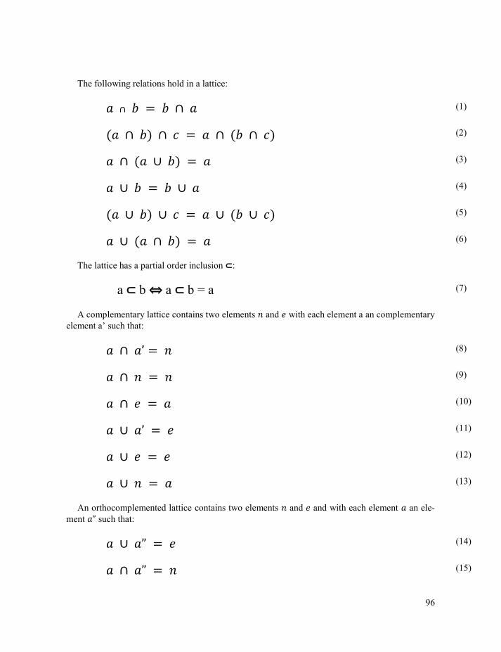
96
The following relations hold in a lattice:
∩ ∩
∩ ∩ ∩ ∩
∩ ∪
∪ ∪
∪ ∪ ∪ ∪
∪ ∩
The lattice has a partial order inclusion :
a b ⇔ a b = a
A complementary lattice contains two elements and with each element a an complementary
element a’ such that:
∩ ’
∩
∩
∪ ’
∪
∪
An orthocomplemented lattice contains two elements and and with each element an ele-
ment such that:
∪
∩
(1)
(2)
(3)
(4)
(5)
(6)
(7)
(8)
(9)
(10)
(11)
(12)
(13)
(14)
(15)
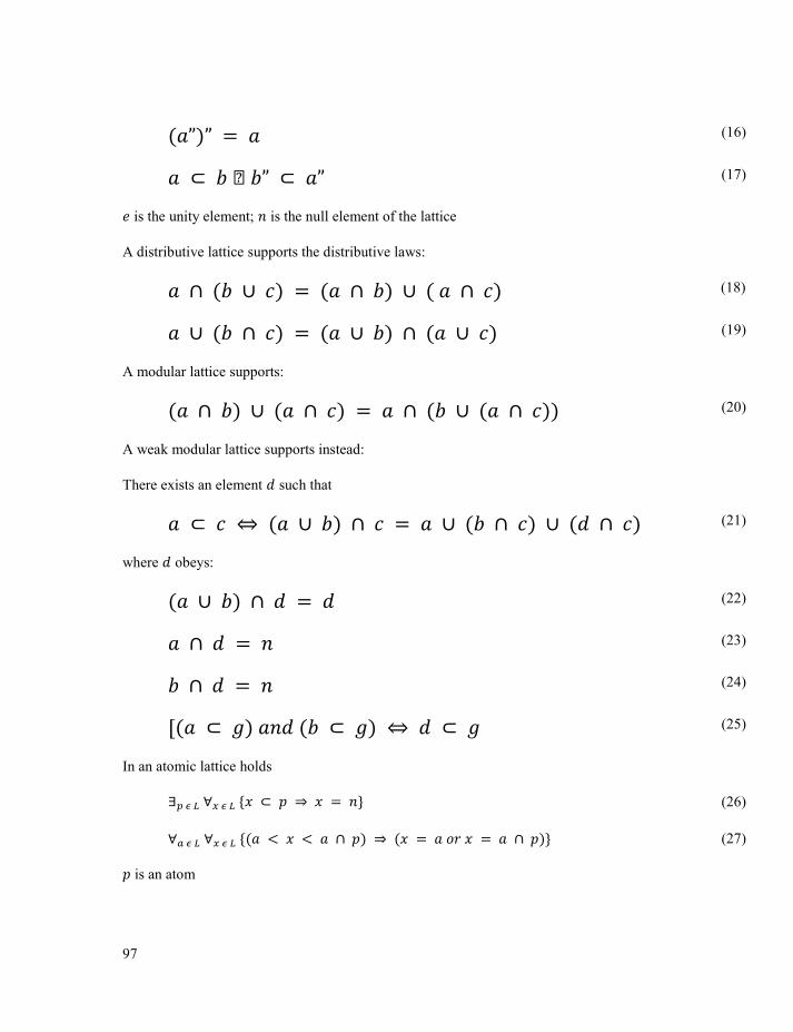
97
is the unity element; is the null element of the lattice
A distributive lattice supports the distributive laws:
∩ ∪ ∩ ∪ ∩
∪ ∩ ∪ ∩ ∪
A modular lattice supports:
∩ ∪ ∩ ∩ ∪ ∩
A weak modular lattice supports instead:
There exists an element such that
⇔ ∪ ∩ ∪ ∩ ∪ ∩
where obeys:
∪ ∩
∩
∩
[ ⇔
In an atomic lattice holds
{ ⇒ }
{ ∩ ⇒ ∩ }
is an atom
(16)
(17)
(18)
(19)
(20)
(21)
(22)
(23)
(24)
(25)
(26)
(27)
98
Both the set of propositions of quantum logic and the set of subspaces of a separable Hilbert
space Ң have the structure of an orthomodular lattice. In this respect these sets are congruent.
In Hilbert space, an atom is a pure state (a ray spanned by a single vector).
Classical logic has the structure of an orthocomplemented distributive modular and atomic lat-
tice.
Quantum logic has the structure of an orthomodular lattice. That is an orthocomplented weakly
modular and atomic lattice. The set of closed subspaces of a Hilbert space also has that structure.
1.2.2 Proposition
In Aristotelian logic a proposition is a particular kind of sentence, one which affirms or denies
a predicate of a subject. Propositions have binary values. They are either true or they are false.
Propositions take forms like "This is a particle or a wave". In quantum logic
"This is a particle." is not a proposition.
In mathematical logic, propositions, also called "propositional formulas"
or "statement forms", are statements that do not contain quantifiers. They
are composed of well-formed formulas consisting entirely of atomic for-
mulas, the five logical connectives88, and symbols of grouping (parenthe-
ses etc.). Propositional logic is one of the few areas of mathematics that is
totally solved, in the sense that it has been proven internally consistent,
every theorem is true, and every true statement can be proved. Predicate
logic is an extension of propositional logic, which adds variables and
quantifiers.
In Hilbert space a vector is either inside or not inside a closed subspace. A
proper quantum logical proposition is “Vector |f> is inside state s”.
In Hilbert space, an atomic predicate corresponds with a subspace that is
spanned be a single vector.
Predicates may accept attributes and quantifiers. The predicate logic is al-
so called first order logic. A dynamic logic can handle the fact that predi-
cates may influence each other when atomic predicates are exchanged.
88 http://en.wikipedia.org/wiki/Logical_connective
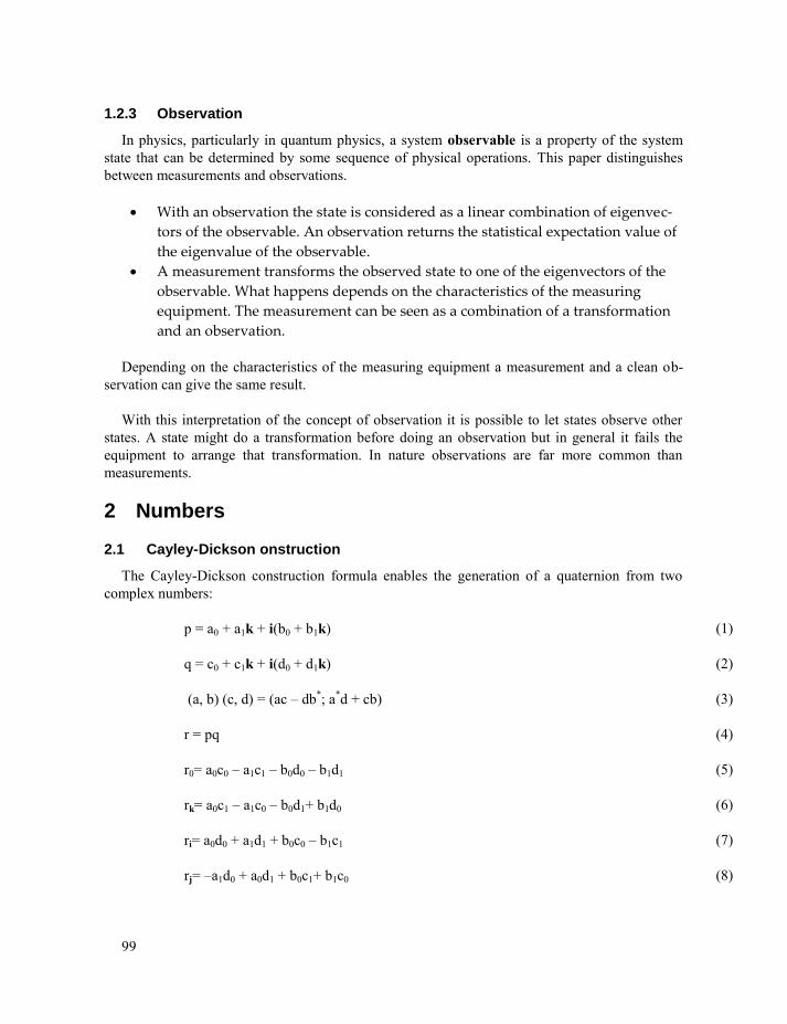
99
1.2.3 Observation
In physics, particularly in quantum physics, a system observable is a property of the system
state that can be determined by some sequence of physical operations. This paper distinguishes
between measurements and observations.
With an observation the state is considered as a linear combination of eigenvec-
tors of the observable. An observation returns the statistical expectation value of
the eigenvalue of the observable.
A measurement transforms the observed state to one of the eigenvectors of the
observable. What happens depends on the characteristics of the measuring
equipment. The measurement can be seen as a combination of a transformation
and an observation.
Depending on the characteristics of the measuring equipment a measurement and a clean ob-
servation can give the same result.
With this interpretation of the concept of observation it is possible to let states observe other
states. A state might do a transformation before doing an observation but in general it fails the
equipment to arrange that transformation. In nature observations are far more common than
measurements.
2 Numbers
2.1 Cayley-Dickson onstruction
The Cayley-Dickson construction formula enables the generation of a quaternion from two
complex numbers:
p = a0 + a1k + i(b0 + b1k)
q = c0 + c1k + i(d0 + d1k)
(a, b) (c, d) = (ac – db*; a
*d + cb)
r = pq
r0= a0c0 – a1c1 – b0d0 – b1d1
rk= a0c1 – a1c0 – b0d1+ b1d0
ri= a0d0 + a1d1 + b0c0 – b1c1
rj= –a1d0 + a0d1 + b0c1+ b1c0
(1)
(2)
(3)
(4)
(5)
(6)
(7)
(8)

100
2.2 Warren Smith’s numbers
All hyper-complex numbers are based on real numbers. Two main construction formulas for
hyper-complex numbers exist. The Cayley-Dickson construction is the most widely known. The
Warren-Smith construction gives best algorithmic properties at higher dimensions. Until the octo-
nions both construction formulas deliver the same results.
The quaternions are the highest dimensional hyper-complex numbers that deliver a division
ring.
2.2.1 2n-on construction
The 2n-ons use the following doubling formula
Up until the 16-ons the formula can be simplified to
Up to the octonions the Cayley Dickson construction delivers the same as the 2
n-on construc-
tion. From n>3 the 2n-ons are ‘nicer’.
2.2.1.1 2n-ons
Table of properties of the 2nons. See www.math.temple.edu/~wds/homepage/nce2.ps.
Ty
pe
name Lose
1o
ns
Reals.
2o
ns
Complex
numbers
z* = z (the * denotes conjugating);
the ordering properties that both {z > 0, -z > 0, or z = 0}
and {w > 0, z > 0 implies w + z > 0, wz > 0}.
4o
ns
Quaterni-
ons
commutativity ab = ba;
the algebraic closedness property that every univariate polynomial
equation has a root.
8o
ns
Octonions associativity ab · c = a · bc.
16
ons
(not Sed-
enions!)
rightalternativity x · yy = xy · y;
rightcancellation x = xy · y-1
;
flexibility x · yx = xy · x; leftlinearity (b + c)a = ba + ca;
antiautomorphism ab = ba, (ab)-1
= b-1
a-1
;
leftlinearity (b + c)a = ba + ca;
continuity of the map x → xy;
Moufang and Bol identities;
diassociativity
32 generalizedsmoothness of the map x → xy;
(1)
(2)
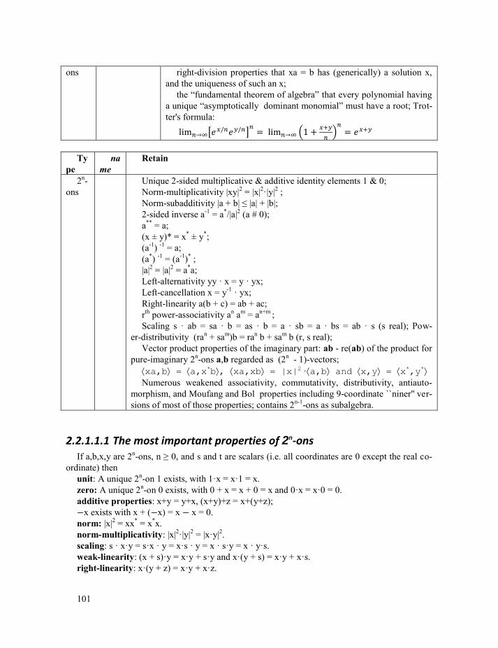
101
ons rightdivision properties that xa = b has (generically) a solution x,
and the uniqueness of such an x;
the “fundamental theorem of algebra” that every polynomial having
a unique “asymptotically dominant monomial” must have a root; Trot-
ter's formula:
lim [ ]
lim (
)
Ty
pe
na
me
Retain
2n
ons
Unique 2sided multiplicative & additive identity elements 1 & 0;
Normmultiplicativity |xy|2 = |x|
2·|y|
2 ;
Normsubadditivity |a + b| ≤ |a| + |b|;
2sided inverse a-1
= a*/|a|
2 (a # 0);
a**
= a;
(x ± y)* = x* ± y
*;
(a-1
) -1
= a;
(a*)
-1 = (a
-1)
* ;
|a|2 = |a|
2 = a
*a;
Leftalternativity yy · x = y · yx;
Leftcancellation x = y-1
· yx;
Rightlinearity a(b + c) = ab + ac;
rth
powerassociativity an a
m = a
n+m ;
Scaling s · ab = sa · b = as · b = a · sb = a · bs = ab · s (s real); Pow-
erdistributivity (ran + sa
m)b = ra
n b + sa
m b (r, s real);
Vector product properties of the imaginary part: ab - re(ab) of the product for
pureimaginary 2nons a,b regarded as (2
n - 1)vectors;
xa,b = a,x*b, xa,xb = |x|2·a,b and x,y = x*,y*
Numerous weakened associativity, commutativity, distributivity, antiauto-
morphism, and Moufang and Bol properties including 9coordinate ``niner'' ver-
sions of most of those properties; contains 2n-1
ons as subalgebra.
2.2.1.1.1 The most important properties of 2n-ons If a,b,x,y are 2
n-ons, n ≥ 0, and s and t are scalars (i.e. all coordinates are 0 except the real co-
ordinate) then
unit: A unique 2n-on 1 exists, with 1·x = x·1 = x.
zero: A unique 2n-on 0 exists, with 0 + x = x + 0 = x and 0·x = x·0 = 0.
additive properties: x+y = y+x, (x+y)+z = x+(y+z);
x exists with x + ( x) = x x = 0.
norm: |x|2 = xx
* = x
*x.
norm-multiplicativity: |x|2·|y|
2 = |x·y|
2.
scaling: s · x·y = s·x · y = x·s · y = x · s·y = x · y·s.
weak-linearity: (x + s)·y = x·y + s·y and x·(y + s) = x·y + x·s.
right-linearity: x·(y + z) = x·y + x·z.
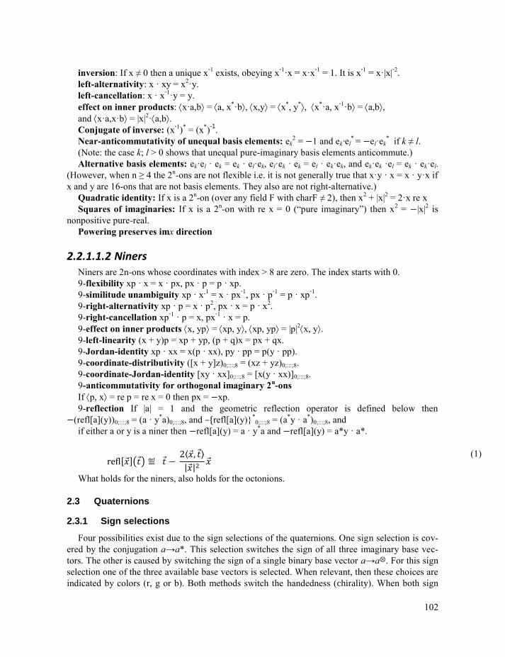
102
inversion: If x ≠ 0 then a unique x-1
exists, obeying x-1
·x = x·x-1
= 1. It is x-1
= x·|x|-2
.
left-alternativity: x · xy = x2·y.
left-cancellation: x · x-1
·y = y.
effect on inner products: x·a,b = a, x*·b, x,y = x
*, y
*, x
*·a, x
-1·b = a,b,
and x·a,x·b = |x|2·a,b.
Conjugate of inverse: (x-1
)* = (x
*)-1
.
Near-anticommutativity of unequal basis elements: ek2 = 1 and ek·el
* = el·ek
* if k ≠ l.
(Note: the case k; l > 0 shows that unequal pure-imaginary basis elements anticommute.)
Alternative basis elements: ek·el · ek = ek · el·ek, el·ek · ek = el · ek·ek, and ek·ek ·el = ek · ek·el.
(However, when n ≥ 4 the 2n-ons are not flexible i.e. it is not generally true that x·y · x = x · y·x if
x and y are 16-ons that are not basis elements. They also are not right-alternative.)
Quadratic identity: If x is a 2n-on (over any field F with charF ≠ 2), then x
2 + |x|
2 = 2·x re x
Squares of imaginaries: If x is a 2n-on with re x = 0 (“pure imaginary”) then x
2 = |x|
2 is
nonpositive pure-real.
Powering preserves imx direction
2.2.1.1.2 Niners Niners are 2n-ons whose coordinates with index > 8 are zero. The index starts with 0.
9-flexibility xp · x = x · px, px · p = p · xp.
9-similitude unambiguity xp · x-1 = x · px-1
, px · p-1
= p · xp-1
.
9-right-alternativity xp · p = x · p2, px · x = p · x
2.
9-right-cancellation xp-1
· p = x, px-1
· x = p.
9-effect on inner products x, yp = xp, y, xp, yp = |p|2x, y.
9-left-linearity (x + y)p = xp + yp, (p + q)x = px + qx.
9-Jordan-identity xp · xx = x(p · xx), py · pp = p(y · pp).
9-coordinate-distributivity ([x + y]z)0;:::;8 = (xz + yz)0;:::;8.
9-coordinate-Jordan-identity [xy · xx]0;:::;8 = [x(y · xx)]0;:::;8.
9-anticommutativity for orthogonal imaginary 2n-ons
If p, x = re p = re x = 0 then px = xp.
9-reflection If |a| = 1 and the geometric reflection operator is defined below then
(refl[a](y))0;:::;8 = (a · y*a)0;:::;8, and {refl[a](y)}
*0;:::;8 = (a
*y · a
*)0;:::;8, and
if either a or y is a niner then refl[a](y) = a · y*a and refl[a](y) = a*y · a*.
refl[ ]( ) ⟨ ⟩
| |
What holds for the niners, also holds for the octonions.
2.3 Quaternions
2.3.1 Sign selections
Four possibilities exist due to the sign selections of the quaternions. One sign selection is cov-
ered by the conjugation a→a*. This selection switches the sign of all three imaginary base vec-
tors. The other is caused by switching the sign of a single binary base vector a→a⊗. For this sign
selection one of the three available base vectors is selected. When relevant, then these choices are
indicated by colors (r, g or b). Both methods switch the handedness (chirality). When both sign
(1)
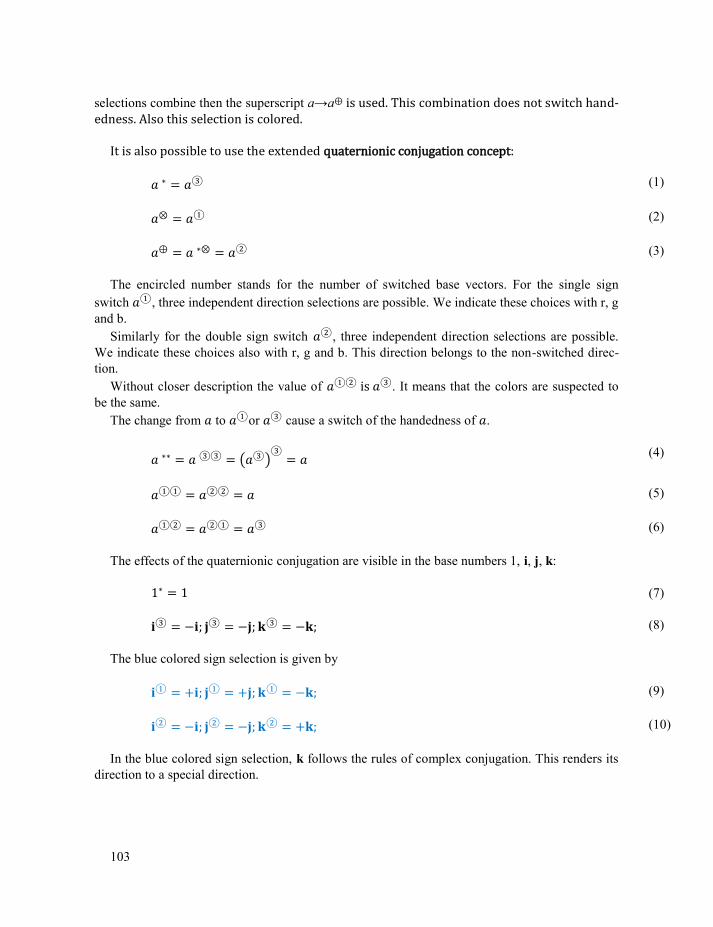
103
selections combine then the superscript a→a⊕ is used. This combination does not switch hand-edness. Also this selection is colored.
It is also possible to use the extended quaternionic conjugation concept:
⊗
⊕ ⊗
The encircled number stands for the number of switched base vectors. For the single sign
switch , three independent direction selections are possible. We indicate these choices with r, g
and b.
Similarly for the double sign switch , three independent direction selections are possible.
We indicate these choices also with r, g and b. This direction belongs to the non-switched direc-
tion.
Without closer description the value of is . It means that the colors are suspected to
be the same.
The change from to or cause a switch of the handedness of .
( )
The effects of the quaternionic conjugation are visible in the base numbers 1, i, j, k:
; ; ;
The blue colored sign selection is given by
; ; ;
; ; ;
In the blue colored sign selection, k follows the rules of complex conjugation. This renders its
direction to a special direction.
(1)
(2)
(3)
(4)
(5)
(6)
(7)
(8)
(9)
(10)
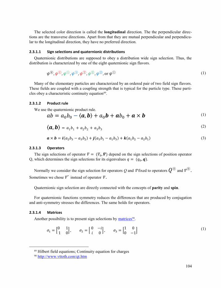
104
The selected color direction is called the longitudinal direction. The the perpendicular direc-
tions are the transverse directions. Apart from that they are mutual perpendicular and perpendicu-
lar to the longitudinal direction, they have no preferred direction.
2.3.1.1 Sign selections and quaternionic distributions
Quaternionic distributions are supposed to obey a distribution wide sign selection. Thus, the
distribution is characterized by one of the eight quaternionic sign flavors.
or
Many of the elementary particles are characterized by an ordered pair of two field sign flavors.
These fields are coupled with a coupling strength that is typical for the particle type. These parti-
cles obey a characteristic continuity equation89.
2.3.1.2 Product rule
We use the quaternionic product rule.
⟨ ⟩
⟨ ⟩
2.3.1.3 Operators
The sign selections of operator depend on the sign selections of position operator
Q, which determines the sign selections for its eigenvalues .
Normally we consider the sign selection for operators Q and fixed to operators and .
Sometimes we chose instead of operator .
Quaternionic sign selection are directly connected with the concepts of parity and spin.
For quaternionic functions symmetry reduces the differences that are produced by conjugation
and anti-symmetry stresses the differences. The same holds for operators.
2.3.1.4 Matrices
Another possibility is to present sign selections by matrices90.
[ ] [
] [
]
89 Hilbert field equations; Continuity equation for charges 90 http://www.vttoth.com/qt.htm
(1)
(1)
(2)
(3)
(1)
105
The matrix switches the complex fields that together form the quaternion field.
[ ] [ ] [ ]
The matrix switches the real parts and the imaginary parts of the complex fields that togeth-
er form the quaternion field and it switches both fields.
[ ] [
] [ ]
The matrix switches the sign of the first complex field.
[ ] [
] [ ]
The Pauli matrices are involutory.
The determinants91 and traces92 of the Pauli matrices are:
det
Tr
[
]
[
]
[
]
[
]
[ ]
The matrices together select the imaginary base vectors. The matrix exchanges the sign of
all imaginary base vectors. Thus the matrix implements the quaternionic conjugate. The conju-
gation also exchanges right handedness against left handedness.
91 http://en.wikipedia.org/wiki/Determinant 92 http://en.wikipedia.org/wiki/Trace_of_a_matrix
(2)
(3)
(4)
(5)
(6)
(7)
(8)
(9)
(10)
(11)
(12)
106
Another way of exchanging right handedness against left handedness is the exchange of the
sign of one of the imaginary base vectors.
[ ] [ ] [ ]
[ ]
The gamma matrices93 translate directly from complex fields to fully featured quaternionic
fields. In this way four sign flavors of quaternionic fields are constructed from four complex
fields. This is represented by four dimensional matrices and four dimensional spinors. The equiva-
lent of the matrix is the matrix.
[
] [
] [
]
It is false to interpret the matrices as vectors. They form a shorthand for handling spinors.
The Pauli matrix represents the sign selection a→a⊗, while the matrix represents the sign
selection a→a*. The other Pauli matrices and the matrices implement the resulting part of the
quaternion behavior for spinors.
2.3.2 Colored signs
In the following text, the consequences for the product of the sign choices of the conjugate
is indicated by blue color . The extra consequence for the product of the choice of the hand-
edness of the cross product is indicated by red color . The mixed sign selection acts on both sign colors.
The handedness can be switched by changing the sign of all imaginary base vectors.
The sign selections split the ring of quaternions in four different realizations.
2.3.3 Waltz details
The 16-ons lose the continuity of the map ⇒ . Also, in general holds ≠ for 16-ons. However, for all 2
n-ons the base numbers fulfill . All 2
n-ons fea-
ture a conjugate and an inverse. The inverse only exists for non-zero numbers. The 2n-ons support
the number waltz
.
93 Appendix; Gamma matrices
(13)
(14)
(15)
(1)
(1)
107
Often the number waltz appears as a unitary number waltz
where is a unit size number and is its conjugate = 1.
In quaternion space the quaternion waltz can be written as
‖ ‖ ‖ ‖
Another way of specifying the difference is:
‖ ‖ ‖ ‖ ‖ ‖
(2)
(3)
(4)
(5)
(6)
(7)
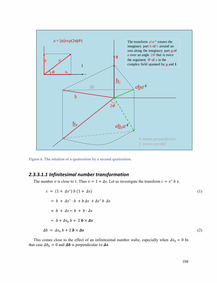
108
a
b||
2Φ
ab#a-1
b
b#
aa
aτΦ
aba-1
The transform aba-1 rotates the
imaginary part b of b around an
axis along the imaginary part a of
a over an angle 2Φ that is twice
the argument Φ of a in the
complex field spanned by a and 11
a = ||a||exp(2πiΦ)
Δb
# means perpendicular
|| means parallel
Figure 6. The rotation of a quaternion by a second quaternion.
2.3.3.1.1 Infinitesimal number transformation The number is close to 1. Thus . Let us investigate the transform .
This comes close to the effect of an infinitesimal number waltz, especially when In
that case and is perpendicular .
(1)
(2)
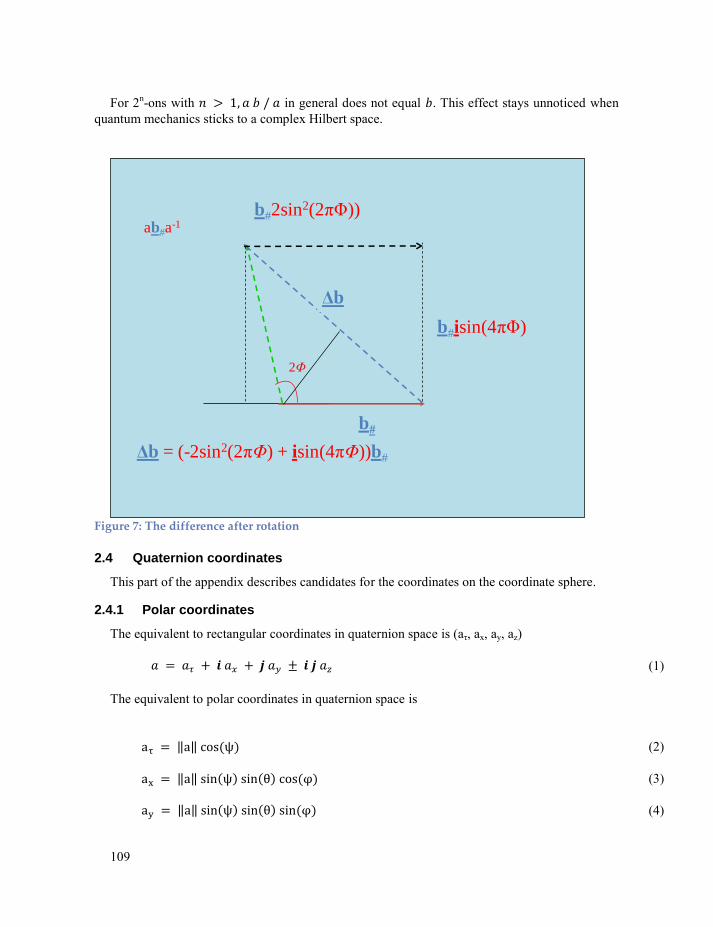
109
For 2n-ons with in general does not equal . This effect stays unnoticed when
quantum mechanics sticks to a complex Hilbert space.
b#
2Φ
Δb
ab#a-1
b#2sin2(2πΦ))
b#isin(4πΦ)
Δb = (-2sin2(2πΦ) + isin(4πΦ))b#
Figure 7: The difference after rotation
2.4 Quaternion coordinates
This part of the appendix describes candidates for the coordinates on the coordinate sphere.
2.4.1 Polar coordinates
The equivalent to rectangular coordinates in quaternion space is (aτ, ax, ay, az)
The equivalent to polar coordinates in quaternion space is
a ‖a‖ cos ψ
a ‖a‖ sin ψ sin cos φ
a ‖a‖ sin ψ sin sin φ
(1)
(2)
(3)
(4)
110
‖ ‖
, where , is known as the (imaginary) amplitude of the quaternion.
Angle is the (co-)latitude and angle is the longitude.
For any fixed value of and parameterize a 2-sphere of radius , except for the de-
generate cases, when equals or , in which case they describe a point.
This suggests the following structure of the argument
‖ ‖
‖ ‖
‖ ‖
The imaginary number may take any direction.
2.4.2 3 sphere
A 3-sphere is a compact, connected, 3-dimensional manifold without boundary. It is also simp-
ly-connected. What this means, loosely speaking, is that any loop, or circular path, on the 3-
sphere can be continuously shrunk to a point without leaving the 3-sphere. The Poincaré conjec-
ture94 proposes that the 3-sphere is the only three dimensional manifold with these properties (up
to homeomorphism)95.
The round metric on the 3-sphere in these coordinates is given by
The volume form is given by
The 3-dimensional volume (or hyperarea) of a 3-sphere of radius r is
The 4-dimensional hypervolume (the volume of the 4-dimensional region bounded by the 3-
sphere) is
The 3-sphere has constant positive sectional curvature equal to . The 3-sphere has a natural Lie group structure SU(2) given by quaternion multiplication.
94 http://en.wikipedia.org/wiki/Poincar%C3%A9_conjecture 95 http://en.wikipedia.org/wiki/3-sphere
(5)
(6)
(7)
(8)
(1)
(2)
(3)
(4)
111
The 3-sphere admits non-vanishing vector fields (sections of its tangent bundle). One can even
find three linearly-independent and non-vanishing vector fields. These may be taken to be any
left-invariant vector fields forming a basis for the Lie algebra of the 3-sphere. This implies that
the 3-sphere is parallelizable. It follows that the tangent bundle of the 3-sphere is trivial.
There is an interesting action of the circle group on giving the 3-sphere the structure of a
principal circle bundle known as the Hopf bundle. If one thinks of as a subset of , the action
is given by
.
The orbit space of this action is homeomorphic to the two-sphere . Since is not homeo-
morphic to , the Hopf bundle is nontrivial.
2.4.3 Hopf coordinates
Another choice of hyperspherical coordinates, , makes use of the embedding of in
. In complex coordinates we write
Here runs over the range 0 to , and and can take any values between 0 and . The-
se coordinates are useful in the description of the 3-sphere as the Hopf bundle
→ →
For any fixed value of η between 0 and , the coordinates parameterize a 2-
dimensional torus. In the degenerate cases, when equals 0 or , these coordinates describe a
circle.
The round metric on the 3-sphere in these coordinates is given by
and the volume form by
2.4.4 Group structure
Because the set of unit quaternions is closed under multiplication, takes on the structure of a
group. Moreover, since quaternionic multiplication is smooth, can be regarded as a real Lie
group. It is a non-abelian, compact Lie group of dimension 3. When thought of as a Lie group is often denoted or .
It turns out that the only spheres which admit a Lie group structure are , thought of as the set
of unit complex numbers, and , the set of unit quaternions. One might think that , the set of
unit octonions, would form a Lie group, but this fails since octonion multiplication is non-
(5)
(1)
(2)
(3)
(4)
(5)
112
associative. The octonionic structure does give one important property: parallelizability96. It
turns out that the only spheres which are parallelizable are , , and . By using a matrix representation of the quaternions, , one obtains a matrix representation of
. One convenient choice is given by the Pauli matrices:
( ) [
]
This map gives an injective algebra homomorphism from H to the set of 2×2 complex matri-
ces. It has the property that the absolute value of a quaternion q is equal to the square root of the
determinant of the matrix image of q.
The set of unit quaternions is then given by matrices of the above form with unit determinant.
This matrix subgroup is precisely the special unitary group SU(2). Thus, as a Lie group is iso-
morphic to SU(2).
Using our hyperspherical coordinates we can then write any element of SU(2) in the
form
[e p sin e p cos e p cos e p sin
]
Another way to state this result is if we express the matrix representation of an element of
SU(2) as a linear combination of the Pauli matrices. It is seen that an arbitrary element U SU(2)
can be written as
∑
The condition that the determinant of U is +1 implies that the coefficients are constrained
to lie on a 3-sphere.
2.4.5 Versor
Any unit quaternion can be written as a versor:
This is the quaternionic analogue of Euler's formula. Now the unit imaginary quaternions all lie
on the unit 2-sphere in Im so any such ĩ can be written:
2.4.6 Symplectic decomposition
Quaternions can be written as the combination of two complex numbers and an imaginary
number k with unit length.
96 http://en.wikipedia.org/wiki/Parallelizability
(1)
(2)
(3)
(1)
(2)
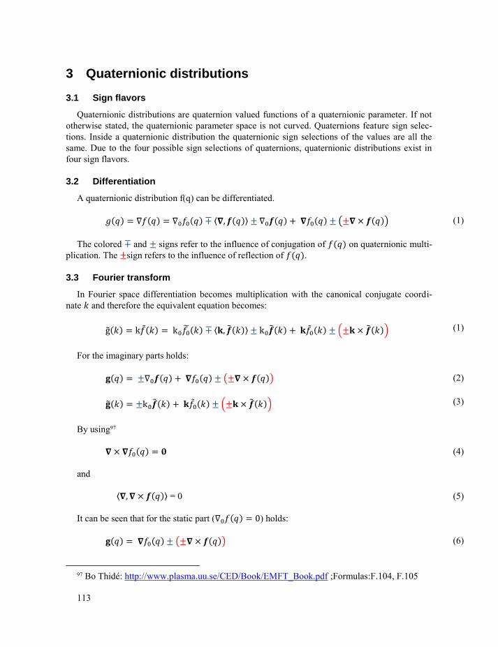
113
3 Quaternionic distributions
3.1 Sign flavors
Quaternionic distributions are quaternion valued functions of a quaternionic parameter. If not
otherwise stated, the quaternionic parameter space is not curved. Quaternions feature sign selec-
tions. Inside a quaternionic distribution the quaternionic sign selections of the values are all the
same. Due to the four possible sign selections of quaternions, quaternionic distributions exist in
four sign flavors.
3.2 Differentiation
A quaternionic distribution f(q) can be differentiated.
⟨ ⟩ ( )
The colored and signs refer to the influence of conjugation of on quaternionic multi-
plication. The sign refers to the influence of reflection of .
3.3 Fourier transform
In Fourier space differentiation becomes multiplication with the canonical conjugate coordi-
nate and therefore the equivalent equation becomes:
g ⟨ ⟩ ( )
For the imaginary parts holds:
( )
( )
By using97
and
⟨ ⟩ = 0
It can be seen that for the static part ( ) holds:
( )
97 Bo Thidé: http://www.plasma.uu.se/CED/Book/EMFT_Book.pdf ;Formulas:F.104, F.105
(1)
(1)
(2)
(3)
(4)
(5)
(6)
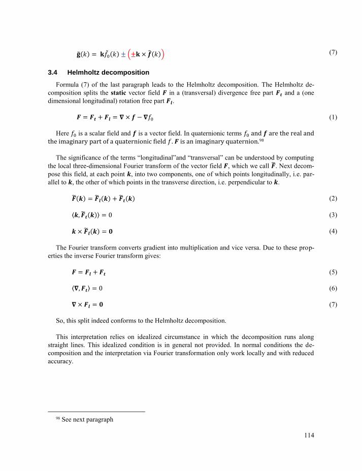
114
( )
3.4 Helmholtz decomposition
Formula (7) of the last paragraph leads to the Helmholtz decomposition. The Helmholtz de-
composition splits the static vector field in a (transversal) divergence free part and a (one
dimensional longitudinal) rotation free part .
Here is a scalar field and is a vector field. In quaternionic terms and are the real and the imaginary part of a quaternionic field . is an imaginary quaternion.98
The significance of the terms “longitudinal”and “transversal” can be understood by computing
the local three-dimensional Fourier transform of the vector field , which we call . Next decom-
pose this field, at each point , into two components, one of which points longitudinally, i.e. par-
allel to , the other of which points in the transverse direction, i.e. perpendicular to .
⟨ ⟩
The Fourier transform converts gradient into multiplication and vice versa. Due to these prop-
erties the inverse Fourier transform gives:
⟨ ⟩
So, this split indeed conforms to the Helmholtz decomposition.
This interpretation relies on idealized circumstance in which the decomposition runs along
straight lines. This idealized condition is in general not provided. In normal conditions the de-
composition and the interpretation via Fourier transformation only work locally and with reduced
accuracy.
98 See next paragraph
(7)
(1)
(2)
(3)
(4)
(5)
(6)
(7)
115
4 Fields
4.1 The origin of physical fields.
The Hilbert Book Model is a simple Higgsless model of physics that is strictly based on tradi-
tional quantum logic and on the lattice isomorphic model; the set of subspaces of an infinite di-
mensional separable Hilbert space for which the inner product is specified by using quaternions99.
This restriction results in the fact that all sets of variables are countable. At the same time most
observations are taken from a continuum. As a result the set of potential observations overwhelms
the set of variables100. The situation is comparable to the situation in which the number of equa-
tions is far larger than the number of variables that should form the result. Probably, the set of
equations will appear to be inconsistent. In order to cure the situation, it is common to assume that
the observations are inaccurate. The inaccuracy must be stochastic or with other words the obser-
vation result must be blurred.
Nature applies a similar solution, but instead of a simple spread function in the form of a prob-
ability density distribution, nature applies a quaternionic probability amplitude distribution
(QPAD). This QPAD can be split into a real part that represents a “charge” density distribution
and an imaginary part that represents a corresponding “current” density distribution. The “charge”
represents the set of properties of the thing that is being observed. The parameter of the distribu-
tion represents the location at which the “charge” is observed. The squared modulus of the QPAD
represents the probability density of the presence of the “charge” at the location that is specified
by the parameter.
This approach transfers the dynamics of the observation into a streaming problem. The equa-
tion of motion of the “charge” becomes a continuity equation101.
The properties of particles move according to the above principle. With each elementary parti-
cle belongs a state function QPAD that act as a private field of the particle and that determines its
dynamic behavior when it moves freely. However, these fields overlap. In this way these fields
and the corresponding particles interact.
A subset of the elementary particles is massless. These particles correspond to a single QPAD.
That does not say that their fields cannot overlap.
All other elementary particles are identified by an ordered pair of QPAD’s that are two field
sign flavors of the same base field. The coordinate system, whose values are used as field parame-
ter, has its own field sign flavor and acts as a sign flavor reference.
4.1.1 Categories of fields
Two categories of fields exist.
4.1.1.1 Primary fields
The first category consists of quaternionic probability amplitude distributions (QPAD’s). The
QPAD’s may overlap and through this superposition they may form covering fields. The QPAD’s
exist in four sign flavors. The same holds for the covering fields. The QPAD’s may interact.
99 See: http://www.crypts-of-physics.eu/HilbertBookModelEssentials.pdf 100 A continuum has a higher cardinality than a countable set. 101 Another name for “continuity equation” is “balance equation”.
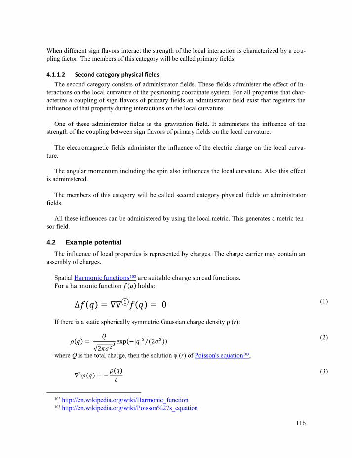
116
When different sign flavors interact the strength of the local interaction is characterized by a cou-
pling factor. The members of this category will be called primary fields.
4.1.1.2 Second category physical fields
The second category consists of administrator fields. These fields administer the effect of in-
teractions on the local curvature of the positioning coordinate system. For all properties that char-
acterize a coupling of sign flavors of primary fields an administrator field exist that registers the
influence of that property during interactions on the local curvature.
One of these administrator fields is the gravitation field. It administers the influence of the
strength of the coupling between sign flavors of primary fields on the local curvature.
The electromagnetic fields administer the influence of the electric charge on the local curva-
ture.
The angular momentum including the spin also influences the local curvature. Also this effect
is administered.
The members of this category will be called second category physical fields or administrator
fields.
All these influences can be administered by using the local metric. This generates a metric ten-
sor field.
4.2 Example potential
The influence of local properties is represented by charges. The charge carrier may contain an
assembly of charges.
Spatial Harmonic functions102 are suitable charge spread functions. For a harmonic function holds:
If there is a static spherically symmetric Gaussian charge density ρ (r):
√ e p | |
⁄
where Q is the total charge, then the solution φ (r) of Poisson's equation103,
102 http://en.wikipedia.org/wiki/Harmonic_function 103 http://en.wikipedia.org/wiki/Poisson%27s_equation
(1)
(2)
(3)
117
is given by
| |erf (| |
√ )
where erf(x) is the error function.
In fact the quaternionic Poisson’s equation represents two separate equations:
Note that, for | | much greater than σ, the erf function approaches unity and the potential φ (r)
approaches the point charge potential
| |, as one would expect. Furthermore the erf function
approaches 1 extremely quickly as its argument increases; in practice for | | > 3σ the relative er-
ror is smaller than one part in a thousand104.
The definition of the quaternionic potential ϕ(q) is based on the convolution of a quaternionic
distribution (q) with the real function See Newton potential and Bertrand’s theorem in
Wikipedia. The real part 0(q) of the distribution (q) can be interpreted as a charge distribution.
The imaginary part (q) can be interpreted as a current distribution.
The convolution blurs the distribution such that the result becomes differentiable.
In configuration space holds:
| |.
Reversely, according to Poisson’s equation:
The real part of ϕ(q) presents a scalar potential. The imaginary part presents a vector potential.
In the above section:
The scalar potential is a blurred charge distribution.
104 http://en.wikipedia.org/wiki/Poisson's_equation#Potential_of_a_Gaussian_charge_density
(4)
(5)
(6)
(7)
(8)
(9)
118
The vector potential is a blurred current distribution.
Current is moving charge.
Mass is a form of charge.
(The selected blurring function has striking resemblance with the ground state of the quantum
harmonic oscillator105).
In Fourier space holds:
| |.
In Fourier space the frequency spectrum of the Hilbert distribution is multiplied with the Fou-
rier transform of the blurring function. When this falls off when the frequencies go to infinity,
then as a consequence the frequency spectrum of the potential is bounded. This is valid independ-
ent of the fact that the frequency spectrum of the Hilbert distribution is unbounded.
5 Fourier transform
5.1 Quaternionic Fourier transform split
The longitudinal Fourier transform represents only part of the full quaternionic Fourier trans-
form. It depends on the selection of a radial line in p space that under ideal conditions runs
along a straight line.
( )
Or
( ) ( )
It relates to the full quaternionic Fourier transform Ƒ
( )
The inverse Fourier transform runs:
The split in longitudinal and transverse Fourier transforms corresponds to a corresponding split
in the multi-dimensional Dirac delta function.
105 Functions and fields:Functions invariant under Fourier transformation:Ladder opera-
tor:Ground state
(10)
(1)
(2)
(3)
(4)
119
We consider a field that equals the quaternionic differentiation of another field with re-
spect to a selected (ideal) coordinate system .
We use the results of the paragraph on decomposition. We only use the static and imaginary
version of field .
For the static imaginary part holds:
( )
In Fourier space differentiation becomes multiplication with the canonical conjugate coordi-
nate and therefore the equivalent equation becomes:
( )
Since
and
⟨ ⟩ ⟨ ⟩
Now we take
| | g
∫ | |
The static imaginary part is
| |
(∫ | |
) ∫ | |
∫ | |
∫ | |
(5)
(6)
(7)
(8)
(9)
(10)
(11)
120
∫ |
∫ |
The left part is the longitudinal inverse Fourier transform of field . The right part is the transverse inverse Fourier transform of field . For the Fourier transform of holds the split:
∫ |
∫ |
∫ |
The longitudinal direction is a one dimensional (radial) space. The corresponding transverse di-
rection is tangent to a sphere in 3D. Its direction depends on the field or alternatively on the
combination of field and the selected (ideal) coordinate system .
For a weakly curved coordinate system the formulas hold with a restricted accuracy and
within a restricted region.
5.2 Alternative transverse plane
The Cayley-Dickson construction, as well as Warren Smith’s construction formula shows that
the transverse part can be considered as a complex number space multiplied with a fixed imagi-
nary quaternionic base number. The selection of the imaginary base number i is arbitrary as long
as it is perpendicular to k. The resulting plane is spanned by axes i and ik. When base number i is
divided away, then a normal complex number space results.
Also here a complex Fourier transform can be defined in a way that is similar to the longitudi-
nal Fourier transform. It must be reckoned that the sign selections for these directions differ.
5.3 Alternative approach to Fourier transform
The following draws from the work of S. Thangavelu106.
Let us take the non-abelian group 1 which is ℝ ⊗ ℝ ⊗ℝ with the group law
; ;
Then it is clear that 1 is non-abelian and the Lebesgue measure dx dy dt is both left and right
invariant Haar measure on 1. With this measure we can form the Hilbert space L2( 1). Let Γ = ℤ
⊗ ℤ ⊗ ℤ. Then it is easy to check that Γ is a subgroup of 1 so that we can form the quotient M
= Γ/ 1 consisting of all right cosets of Γ. Functions on M are naturally identified with left Γ-
invariant functions on 1. As the Lebesgue measure dx dy dt is left Γ-invariant we can form
106 http://www.math.iitb.ac.in/atm/faha1/veluma.pdf
(12)
(1)
121
L2(M) using the Lebesgue measure restricted to M. As a set we can identify M with [0, 1)3 and we
just think of L2(M) as L
2([0, 1)
3).
Fourier expansion in the last variable allows us to decompose L2(M) into a direct sum of or-
thogonal subspaces. Simply define ℋk to be the set of all f ∈L2(M) which satisfy the condition
e p
Then ℋk is orthogonal to ℋj whenever k ≠ j and any f ∈ L2(M) has the unique expansion
∑
; ∈ ℋ
In quaternionic terms, the split sees ik as imaginary quaternion k and the quaternionic Hilbert
space is split in components according to the imaginary direction of k, where the choice is be-
tween three mutually perpendicular directions.
For the moment, we are mainly interested in ℋ1 which is a Hilbert space in its own right. It is
interesting to note that functions in ℋ1 are also invariant under the left action of Γ.
Our next example of a unitary operator is the following. Consider the map J : ℋ1 → ℋ1 given
by
; ;
;
5.4 Weil-Brezin transform
Next consider the Weil-Brezin transform V:
∑ e p
(2)
(3)
(4)
(5)
(6)
(7)
(8)
(9)
(10)
(1)
122
∫ | | ∫ ∑ | |
∭| | ∫ | |
V is unitary.
See also Zak transform
5.5 Fourier transform
We define the Fourier transform F by:
; for every ∈ ℝ
; for almost every ∈ ℝ
‖ ‖ ‖ ‖
For ∈ ℝ ℝ the Fourier transform is given by
f ∫ f e p ∈ ℝ
If we further assume that ∈ ℝ then for almost every x we have
f ∫ f e p ∈ ℝ
5.6 Functions invariant under Fourier transform
In this section we confine to a complex part of the Hilbert space.
See http://en.wikipedia.org/wiki/Hermite_polynomials.
There exist two types of Hermite polynomials:
1. The probalist’s Hermite polynomials:
e p
e p .
2. The physicist’s Hermite polynomials
(2)
(3)
(1)
(2)
(3)
( √ )
(1, 2)
123
e p
e p e p (
) e p
These two definitions are not exactly equivalent; either is a rescaling of the other:
( √ )
In the following we focus on the physicist’s Hermite polynomials.
The Gaussian function φ(z) defined by
is an eigenfunction of F. It means that its Fourier transform has the same form.
As I any λ in its spectrum satisfies λ4 = 1: Hence,
{ ; ; ; }.
We take the Fourier transform of the expansion:
∑
First we take the Fourier transform of the left hand side:
√ ∫
∑
The Fourier transform of the right hand side is given by
√ ∑ ∫
(3)
(4)
(5)
(6)
(7)
(8)
124
Equating like powers of c in the transformed versions of the left- and
right-hand sides gives
√ ∫ e p
e p
Let us define the Hermite functions
| c e p
| |
with suitably chosen cn so as to make
‖ ‖
c
√ √
The importance of the Hermite functions lie in the following theorem.
“The Hermite functions ψn; n N form an orthonormal basis for L2(R)”
Consider the operator
Apply this to ψn(z):
Thus, ψn is an eigenfunction of H.
Let f ψ be any of the Hermite functions. Then we have
∑ e p( )
(9)
(10)
(11)
(12)
(13)
(14)
(15)
(16)
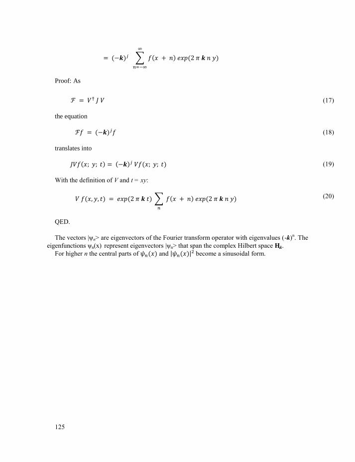
125
∑
Proof: As
the equation
translates into
; ; ; ;
With the definition of V and t = xy:
∑
QED.
The vectors |ψn> are eigenvectors of the Fourier transform operator with eigenvalues (-k)n. The
eigenfunctions ψn(x) represent eigenvectors |ψn> that span the complex Hilbert space Ңk.
For higher n the central parts of and | | become a sinusoidal form.
(17)
(18)
(19)
(20)
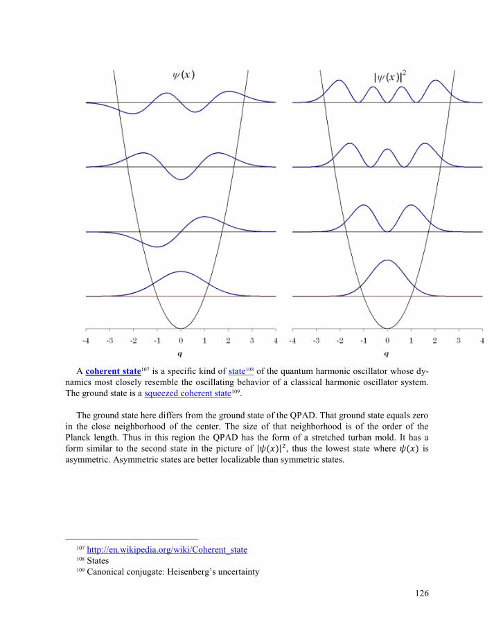
126
A coherent state107 is a specific kind of state108 of the quantum harmonic oscillator whose dy-
namics most closely resemble the oscillating behavior of a classical harmonic oscillator system.
The ground state is a squeezed coherent state109.
The ground state here differs from the ground state of the QPAD. That ground state equals zero
in the close neighborhood of the center. The size of that neighborhood is of the order of the
Planck length. Thus in this region the QPAD has the form of a stretched turban mold. It has a
form similar to the second state in the picture of | | , thus the lowest state where is
asymmetric. Asymmetric states are better localizable than symmetric states.
107 http://en.wikipedia.org/wiki/Coherent_state 108 States 109 Canonical conjugate: Heisenberg’s uncertainty

127
5.7 Special Fourier transform pairs
Functions that keep the same form through Fourier transformation are:
e p | |
| |
The comb function consists of a set of equidistant Dirac delta functions.
Other examples of functions that are invariant under Fourier transformation are the linear and
spherical harmonic oscillators and the solutions of the Laplace equation.
5.8 Complex Fourier transform invariance properties
Each even function induces a Fourier invariant:
√ .
√
Each odd function induces a Fourier invariant:
√ .
A function is invariant under Fourier transformation if and only if the function satisfies
the differential equation
, for some scalar ∈ .
The Fourier transform invariant functions are fixed apart from a scale factor. That scale factor
can be 1, k, -1 or –k. k is an imaginary base number in the longitudinal direction.
Fourier-invariant functions show iso-resolution, that is, in the Heisenberg’s uncertain-
ty relation.
For proves see: http://www2.ee.ufpe.br/codec/isoresolution_vf.pdf.
5.9 Fourier transform properties
5.9.1 Parseval’s theorem
Parseval’s theorem runs:
(1)
(2)
(3)
(1)
(2)
(3)
(4)
128
∫ ∫
This leads to
∫| | ∫| |
5.9.2 Convolution
Through Fourier transformation a convolution changes into a simple product and vice versa.
5.9.3 Differentiation
Fourier transformation converts differentiation into multiplication with the canonical conjugat-
ed coordinate.
g
g p
6 Ladder operator
The Hermite functions represent Fock states110.
Boson ladder operators are characterized by
| √ |
| √ |
√ (
) √
√
√ (
) √
√
In the Heisenberg picture, the operators have the following time dependence:
e p( t )
110 http://en.wikipedia.org/wiki/Fock_state
(1)
(2)
(1)
(1)
(2)
(1)
(2)
(3)
129
e p t
We can also define an enumeration operator N which has the following property:
| |
In deriving the form of , we have used the fact that the operators X and Px, which represent
observables, are Hermitian. These observable operators can be expressed as a linear combination
of the ladder operators as
√
√
The and operators obey the following identity, known as the canonical commutation rela-
tion:
[ ]
Using the above, we can prove the identities
[ ]
Now, let |fE>denote an energy eigenstate with energy E. The inner product of any ket with it-
self must be non-negative, so
| |
Expressing in terms of the Hamiltonian H:
|
so that
.
Note that when | | (is the zero ket i.e. a ket with length zero), the inequality is
saturated, so that
(4)
(5)
(6)
(7)
(8)
(9)
(10)
(11)
(12)
(13)
(14)
130
It is straightforward to check that there exists a state satisfying this condition; it is the ground
state
| | ;
Using the above identities, we can now show that the commutation relations of and with
H are:
[ ]
[ ]
Thus, provided | is not the zero ket,
| |[ ]
|
|
|
Similarly, we can show that
| |
In other words, acts on an eigenstate of energy E to produce, up to a multiplicative constant,
another eigenstate of energy E – ħ ω, and acts on an eigenstate of energy E to produce an ei-
genstate of energy E + ħ ω. For this reason, a is called a "lowering operator", and "raising
operator". The two operators together are called ladder operators. In quantum field theory, and
are alternatively called "annihilation" and "creation" operators because they destroy and create
particles, which correspond to our quanta of energy.
Given any energy eigenstate, we can act on it with the lowering operator , to produce another
eigenstate with ħ ω-less energy. By repeated application of the lowering operator, it seems that we
can produce energy eigenstates down to E = −∞. However, this would contradict our earlier re-
quirement that E ≥ ħ ω/2.
7 States
7.1 Ground state
Therefore, there must be a ground-state energy eigenstate, which we label |fground>, such that
| | ; (zero ket).
(15)
(16)
(17)
(18)
(19)
(20)
(1)
131
In this case, subsequent applications of the lowering operator will just produce zero kets, in-
stead of additional energy eigenstates. Furthermore, we have shown above that
| |
Finally, by acting on | with the raising operator and multiplying by suitable normal-
ization factors, we can produce an infinite set of energy eigenstates
{| | | . | },
such that
| |
which matches the energy spectrum.
This method can also be used to quickly find the ground state state function of the quantum
harmonic oscillator.
Indeed
| |
becomes
|
so that
⇒ ln( )
After normalization this leads to the following position space representation of the ground state
state function.
√
7.2 Coherent state
A coherent state is a specific kind of state111 of the quantum harmonic oscillator112 whose dy-
namics most closely resemble the oscillating behavior of a classical harmonic oscillator system.
111States 112 Functions invariant under Fourier transform
(2)
(3)
(4)
(5)
(6)
(7)
(8)
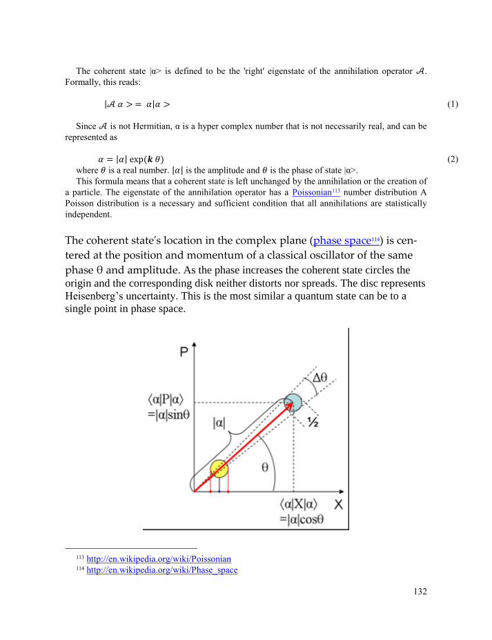
132
The coherent state |α> is defined to be the 'right' eigenstate of the annihilation operator .
Formally, this reads:
| |
Since is not Hermitian, α is a hyper complex number that is not necessarily real, and can be
represented as
| | e p where is a real number. | | is the amplitude and is the phase of state |α>.
This formula means that a coherent state is left unchanged by the annihilation or the creation of
a particle. The eigenstate of the annihilation operator has a Poissonian113 number distribution A
Poisson distribution is a necessary and sufficient condition that all annihilations are statistically
independent.
The coherent state's location in the complex plane (phase space114) is cen-
tered at the position and momentum of a classical oscillator of the same
phase θ and amplitude. As the phase increases the coherent state circles the
origin and the corresponding disk neither distorts nor spreads. The disc represents
Heisenberg’s uncertainty. This is the most similar a quantum state can be to a
single point in phase space.
113 http://en.wikipedia.org/wiki/Poissonian 114 http://en.wikipedia.org/wiki/Phase_space
(1)
(2)
133
Phase space plot of a coherent state. This shows that the uncertainty (blur) in a coherent state is
equally distributed in all directions. The horizontal and vertical axes are the X and P quadratures
of the field, respectively. Oscillations that are said to be in quadrature, if they are separated in
phase by π/2 radians. The red dots on the x-axis trace out the boundaries of the quantum noise.
Further from the origin the relative contribution of the quantum noise becomes less important.
The representation of the coherent state in the basis of Fock states is:
| e p | | ∑
√
| e p | | e p ( ) |
where |n> are Hermite functions (eigenvectors of the Hamiltonian). This is a Poissonian distri-
bution. The probability of detecting n photons is:
e p ⟨ ⟩ ⟨ ⟩
Similarly, the average photon number in a coherent state is
⟨ ⟩ ⟨ ⟩ | |
and the variance is
( ) | |
7.3 Squeezing
The squeezing operator can squeeze a state more or less in the direction of either P or Q. The
operator is defined as:
e p ( ( ))
e p
The ground state is a saturated squeezed coherent state where
and Δq·Δp = ħ/2
8 Base transforms
Now we have discovered the following base transforms:
Position momentum:
(3)
(4)
(5)
(6)
(1)
(2)
(3)
134
|
√ e p
Position Foc state:
| √
√ e p
√
Fock state coherent state:
|
√ e p | |
9 Oscillations
9.1 Harmonic oscillating Hilbert field
Take the ingredients of the complex harmonic oscillator and interpret these as similar ingredi-
ents of a harmonic oscillating Hilbert field that is based on a Gaussian blur. The blur delivers the
conditions of the ground state.
√
This means that the ground state corresponds with a Gaussian charge distribution. Higher states
correspond to a blurred current. We indicate this current as vector potential . Its time derivative
is perpendicular to . The other ingredients are P, Q, and .
√
√
√
(
) √
(
)
√
(
) √
(
)
(1)
(2)
(3)
(1)
(2)
(3)
(4)
(5)
(6)
(7)
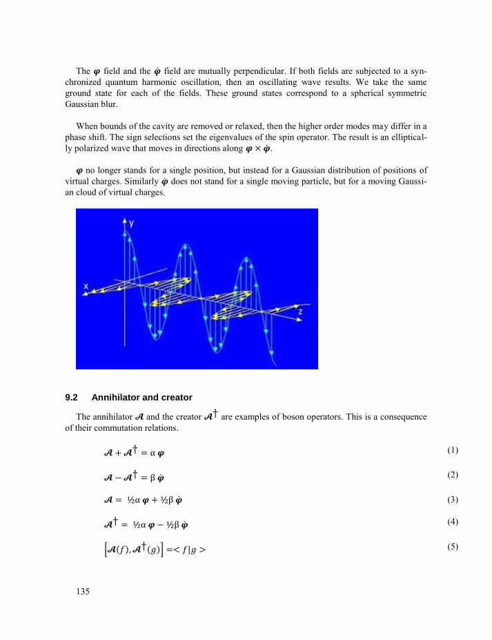
135
The field and the field are mutually perpendicular. If both fields are subjected to a syn-
chronized quantum harmonic oscillation, then an oscillating wave results. We take the same
ground state for each of the fields. These ground states correspond to a spherical symmetric
Gaussian blur.
When bounds of the cavity are removed or relaxed, then the higher order modes may differ in a
phase shift. The sign selections set the eigenvalues of the spin operator. The result is an elliptical-
ly polarized wave that moves in directions along .
no longer stands for a single position, but instead for a Gaussian distribution of positions of
virtual charges. Similarly does not stand for a single moving particle, but for a moving Gaussi-
an cloud of virtual charges.
9.2 Annihilator and creator
The annihilator and the creator are examples of boson operators. This is a consequence
of their commutation relations.
α
β
α β
α β
[ ] |
(1)
(2)
(3)
(4)
(5)
136
[ ]
[ ]
The corresponding fermion operators are:
{ } |
{ }
{ }
The fermion operators can be represented by imaginary quaternionic base numbers:
( ) ( )
9.3 Rotational symmetry
In case of rotational symmetry in the imaginary part of quaternion space, the exponential func-
tion must be replaced by a Bessel function. The corresponding Fourier transform then becomes a
Hankel transform115.
The spherical harmonics are eigenfunctions of the square of the orbital
angular momentum operator and therefore they represent the
different quantized configurations of atomic orbitals.
9.4 Spherical harmonics
The following draws from the work of S. Thangavelu116.
115 http://en.wikipedia.org/wiki/Hankel_transform 116 http://www.math.iitb.ac.in/atm/faha1/veluma.pdf
(6)
(7)
(8)
(9)
(10)
(11)
(12)
(13)
(14)
(15)
137
In this subsection we look for eigenfunctions of the Fourier transform which have spherical
symmetry. As in the one dimensional case we consider functions of the form
e p | |
This will be an eigenfunction of if and only satisfies
∫ e p | | ℝ
Here in quaternion terms and represent two mutually perpendicular imaginary numbers
while and are parallel. Thangavelu uses complex numbers. We keep as close as is possible to
his text.
If (2) is true for all ∈ ℝ then we should also have
∫ e p | | ℝ
Integrating in polar coordinates the integral on the left is
∫ | | (∫
)
where is the normalised surface measure on the unit sphere .
If is homogeneous of degree m then
and hence for such polynomials the equation
∫ e p | | ℝ
will be satisfied for
if has the mean value property
∫
Such functions are precisely the harmonic functions satisfying
(1)
(2)
(3)
(4)
(5)
(6)
(7)
(8)
138
Thus we have proved:
Let
| |
where is homogeneous of degree m and harmonic. Then
Let stand for the finite dimensional space of homogeneous harmonic polynomials of de-
gree m:
The above theorem says that the finite dimensional subspace of ℝ consisting of functions
of the form
e p | | ; ∈
is invariant under the Fourier transform.
We claim that the following extension is true.
Let
∈ ℝ
be of the form
| | ; ∈ Then
| |
Thus the subspace of functions of the form
| | ; ∈
is invariant under the Fourier transform.
Let
∈ ℝ
be of the form
(9)
(10)
(11)
(12)
(13)
(14)
(15)
(16)
(17)
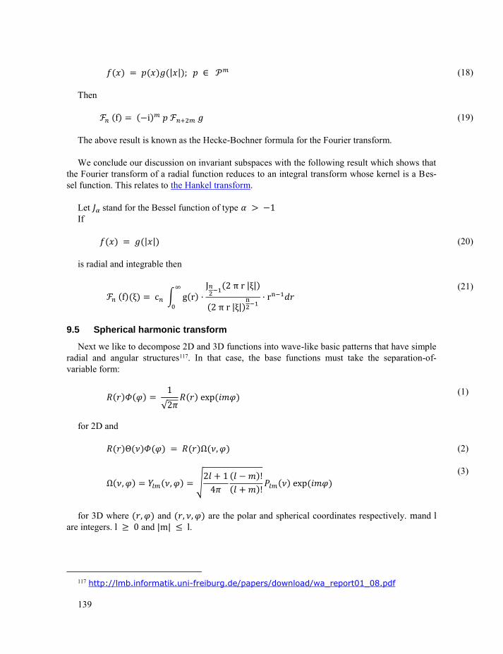
139
| | ; ∈
Then
f i
The above result is known as the Hecke-Bochner formula for the Fourier transform.
We conclude our discussion on invariant subspaces with the following result which shows that
the Fourier transform of a radial function reduces to an integral transform whose kernel is a Bes-
sel function. This relates to the Hankel transform.
Let stand for the Bessel function of type If
| |
is radial and integrable then
f c ∫ g r r | |
r | | r
9.5 Spherical harmonic transform
Next we like to decompose 2D and 3D functions into wave-like basic patterns that have simple
radial and angular structures117. In that case, the base functions must take the separation-of-
variable form:
√ e p
for 2D and
√
e p
for 3D where and are the polar and spherical coordinates respectively. mand l are integers. l and |m| l.
117 http://lmb.informatik.uni-freiburg.de/papers/download/wa_report01_08.pdf
(18)
(19)
(20)
(21)
(1)
(2)
(3)
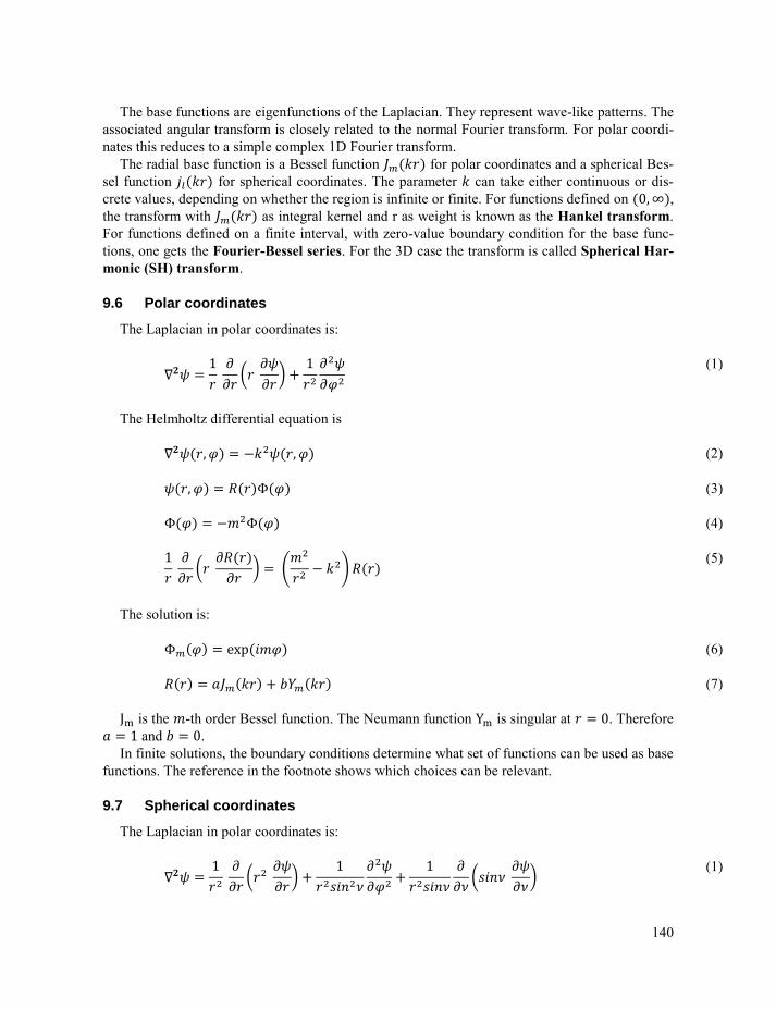
140
The base functions are eigenfunctions of the Laplacian. They represent wave-like patterns. The
associated angular transform is closely related to the normal Fourier transform. For polar coordi-
nates this reduces to a simple complex 1D Fourier transform.
The radial base function is a Bessel function for polar coordinates and a spherical Bes-
sel function for spherical coordinates. The parameter can take either continuous or dis-
crete values, depending on whether the region is infinite or finite. For functions defined on , the transform with as integral kernel and r as weight is known as the Hankel transform.
For functions defined on a finite interval, with zero-value boundary condition for the base func-
tions, one gets the Fourier-Bessel series. For the 3D case the transform is called Spherical Har-
monic (SH) transform.
9.6 Polar coordinates
The Laplacian in polar coordinates is:
(
)
The Helmholtz differential equation is
Φ
Φ Φ
(
) (
)
The solution is:
Φ e p
is the -th order Bessel function. The Neumann function is singular at . Therefore
and . In finite solutions, the boundary conditions determine what set of functions can be used as base
functions. The reference in the footnote shows which choices can be relevant.
9.7 Spherical coordinates
The Laplacian in polar coordinates is:
(
)
(
)
(1)
(2)
(3)
(4)
(5)
(6)
(7)
(1)
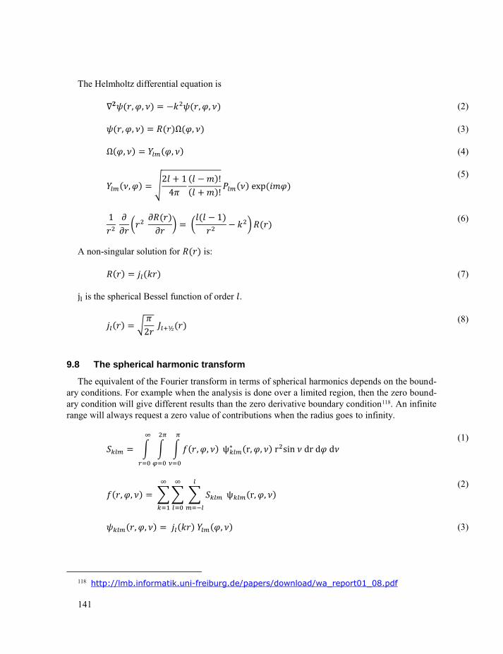
141
The Helmholtz differential equation is
√
e p
(
) (
)
A non-singular solution for is:
is the spherical Bessel function of order .
√
9.8 The spherical harmonic transform
The equivalent of the Fourier transform in terms of spherical harmonics depends on the bound-
ary conditions. For example when the analysis is done over a limited region, then the zero bound-
ary condition will give different results than the zero derivative boundary condition118. An infinite
range will always request a zero value of contributions when the radius goes to infinity.
∫ ∫ ∫
ψ r r sin dr d d
∑∑ ∑
ψ r
118 http://lmb.informatik.uni-freiburg.de/papers/download/wa_report01_08.pdf
(2)
(3)
(4)
(5)
(6)
(7)
(8)
(1)
(2)
(3)
142
9.9 The Fourier transform of a black hole
In its simplest form a black hole is a bubble that is covered with a blanket of ground states.
The blanket is a comb function that is convoluted with a ground state. The Fourier transform of
this blanket is the product of the Fourier transform of the comb function and the Fourier transform
of the ground state. Apart from a factor, the ground state is invariant under Fourier transfor-
mation. Also the comb function is invariant. Thus the Fourier transform of the blanket is a modu-
lated comb function. The modulation does not reach far.
The most complicated component is the bubble. In its simplest form this is a pulse on the radi-
us. If we interpret this pulse as a Dirac delta function, then the Fourier coefficients have the form:
√
If we sum these coefficients, then we get a sampled spherical Bessel function. These spheres
are blurred with the transformed blanket.
9.10 Spherical harmonics eigenvalues
See: http://en.wikipedia.org/wiki/Spherical_harmonics for more details.
Spherical harmonics are best presented in polar coordinates. There exists a corresponding polar
Fourier transform. This Fourier transform also has invariant functions. Like in the rectangular
case, they form the basis for spherical harmonics.
Laplace's equation in spherical coordinates is:
(
)
sin
Try to find solutions in the form of the eigenfunctions of the Fourier transform.
By separation of variables, two differential equations result by imposing Laplace's equation:
(
)
sin
(sin
)
sin
The second equation can be simplified under the assumption that has the form
Applying separation of variables again to the second equation gives way to the pair of differen-
tial equations
(1)
(2)
(3)
(4)
(5)
143
sin sin
[sin
]
for some number m. A priori, m is a complex constant, but because must be a periodic func-
tion whose period evenly divides is necessarily an integer and is a linear combination of
the complex exponentials e p . The solution function is regular at the poles of
the sphere, where . Imposing this regularity in the solution of the second equation at
the boundary points of the domain is a Sturm–Liouville problem119 that forces the parameter to
be of the form for some non-negative integer with | |; this is also explained
below in terms of the orbital angular momentum. Furthermore, a change of variables transforms this equation into the Legendre equation, whose solution is a multiple of the associated
Legendre function120. . Finally, the equation for R has solutions of the form
; requiring the solution to be regular throughout ℝ forces . Here the solution was assumed to have the special form
For a given value of , there are independent solutions of this form, one for each inte-
ger m with . These angular solutions are a product of trigonometric functions, here
represented as a complex exponential, and associated Legendre functions:
e p
which fulfill
Here is called a spherical harmonic function of degree and order m,
is an associated
Legendre function, N is a normalization constant, θ represents the colatitude and φ represents the
longitude. In particular, the colatitude121 θ, or polar angle, ranges from 0 at the North Pole to π at
the South Pole, assuming the value of π/2 at the Equator, and the longitude122 , or azimuth123,
may assume all values with . For a fixed integer , every solution of the ei-
genvalue problem
119 http://en.wikipedia.org/wiki/Sturm%E2%80%93Liouville_problem 120 http://en.wikipedia.org/wiki/Associated_Legendre_function 121 http://en.wikipedia.org/wiki/Colatitude 122 http://en.wikipedia.org/wiki/Longitude 123 http://en.wikipedia.org/wiki/Azimuth
(6)
(7)
(8)
(9)
(10)
(11)
144
is a linear combination of . In fact, for any such solution, is the expression in
spherical coordinates of a homogeneous polynomial that is harmonic, and so counting dimensions
shows that there are linearly independent of such polynomials.
The general solution to Laplace's equation in a ball centered at the origin is a linear combina-
tion of the spherical harmonic functions multiplied by the appropriate scale factor ,
∑ ∑
where the are constants and the factors·
are known as solid harmonics124. Such an ex-
pansion is valid in the ball
lim ⇒ |
|
9.11 Orbital angular momentum
In quantum mechanics, Laplace's spherical harmonics are understood in terms of the orbital
angular momentum125
The spherical harmonics are eigenfunctions of the square of the orbital angular momentum
(
)
sin
sin
sin
Laplace's spherical harmonics are the joint eigenfunctions of the square of the orbital angular
momentum and the generator of rotations about the azimuthal axis:
(
)
These operators commute, and are densely defined self-adjoint operators on the Hilbert space
of functions ƒ square-integrable with respect to the normal distribution on ℝ :
∫ | |
ℝ e p | |
Furthermore, is a positive operator.
124 http://en.wikipedia.org/wiki/Solid_harmonics 125 http://en.wikipedia.org/wiki/Orbital_angular_momentum
(12)
(13)
(1)
(2)
(3)
(4)
145
If is a joint eigenfunction of and , then by definition
for some real numbers m and . Here m must in fact be an integer, for must be periodic in the
coordinate with period a number that evenly divides . Furthermore, since
and each of are self-adjoint, it follows that .
Denote this joint eigenspace by , and define the raising and lowering operators by
Then and commute with , and the Lie algebra generated by is the special
linear Lie algebra, with commutation relations
[ ]
[ ]
[ ]
Thus : (it is a "raising operator") and : (it is a "lowering
operator"). In particular, : must be zero for k sufficiently large, because the ine-
quality must hold in each of the nontrivial joint eigenspaces. Let ∈ be a nonzero
joint eigenfunction, and let k be the least integer such that
Then, since
it follows that
( )
Thus for the positive integer .
(5)
(6)
(7)
(8)
(9)
(10)
(11)
(12)
(13)
(14)
(15)
(16)
146
9.12 Spherical harmonics expansion
The Laplace spherical harmonics form a complete set of orthonormal functions and thus form
an orthonormal basis of the Hilbert space of square-integrable functions. On the unit sphere, any
square-integrable function can thus be expanded as a linear combination of these:
∑ ∑
This expansion holds in the sense of mean-square convergence — convergence in L2 of the
sphere — which is to say that
lim ∫ ∫ | ∑ ∑
|
sin
The expansion coefficients are the analogs of Fourier coefficients, and can be obtained by mul-
tiplying the above equation by the complex conjugate of a spherical harmonic, integrating over
the solid angle , and utilizing the above orthogonality relationships. This is justified rigorously
by basic Hilbert space theory. For the case of orthonormalized harmonics, this gives:
∫
∫ ∫ sin
If the coefficients decay in ℓ sufficiently rapidly — for instance, exponentially — then the se-
ries also converges uniformly to ƒ.
A real square-integrable function ƒ can be expanded in terms of the real harmonics Yℓm above
as a sum
∑ ∑
Convergence of the series holds again in the same sense.
9.13 Spin weighted spherical harmonics
Regard the sphere as embedded into the three-dimensional imaginary
part of the quaternionic number field. At a point x on the sphere, a posi-
tively oriented orthonormal basis of tangent vectors at x is a pair a, b of
vectors such that
(1)
(2)
(3)
(4)
(1)
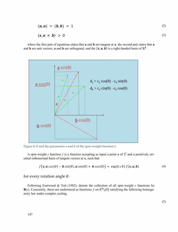
147
⟨ ⟩
where the first pair of equations states that a and b are tangent at x, the second pair states that a
and b are unit vectors, a and b are orthogonal, and the { } is a right-handed basis of ℝ .
θ
a·sin(θ)
a·cos(θ)
b·cos(θ)
-b·sin(θ)
θ
a·sin(θ)
a·cos(θ)
b·cos(θ)-b·sin(θ)
ψ
ψ
c
d
da = ca·cos(θ) –cb·sin(θ)
db = ca·cin(θ) –cb·cos(θ)
Figure 8: θ and the parameters a and b of the spin-weight function f.
A spin-weight s function ƒ is a function accepting as input a point x of S2 and a positively ori-
ented orthonormal basis of tangent vectors at x, such that
( ) e p
for every rotation angle .
Following Eastwood & Tod (1982), denote the collection of all spin-weight s functions by
B(s). Concretely, these are understood as functions ƒ on { } satisfying the following homoge-
neity law under complex scaling
(2)
(3)
(4)
(5)
148
(
)
This makes sense provided s is a half-integer.
Abstractly, B(s) is isomorphic to the smooth vector bundle underlying the antiholomorphic
vector bundle O*(2·s) of the Serre twist on the complex projective line . A section of the latter
bundle is a function g on { } satisfying
( ) ( )
Given such a g, we may produce a spin-weight s function by multiplying by a suitable power
of the Hermitian form
Specifically, is a spin-weight s function. The association of a spin-weighted function
to an ordinary homogeneous function is an isomorphism.
9.14 Eth
The spin weight bundles B(s) are equipped with a differential operator ð (eth). This operator is
essentially the Dolbeault operator126,
Thus for ,
defines a function of spin-weight .
9.15 Spin-weighted harmonic functions
See http://en.wikipedia.org/wiki/Spin-weighted_spherical_harmonics for more details.
Just as conventional spherical harmonics are the eigenfunctions of the Laplace-Beltrami opera-
tor on the sphere, the spin-weight s harmonics are the eigensections for the Laplace-Beltrami op-
erator acting on the bundles of spin-weight s functions.
The spin-weighted harmonics can be represented as functions on a sphere once a point on the
sphere has been selected to serve as the North Pole. By definition, a function η with spin weight s
transforms under rotation about the pole via
e p
126 http://en.wikipedia.org/wiki/Dolbeault_operator
(6)
(7)
(1)
(2)
(1)
149
Working in standard spherical coordinates, we can define a particular operator ð acting on a
function η as:
sin {
sin
}[sin ]
This gives us another function of and . [The operator ð is effectively a covariant derivative
operator in the sphere.]
An important property of the new function is that if η had spin weight has spin weight
. Thus, the operator raises the spin weight of a function by 1. Similarly, we can define an
operator which will lower the spin weight of a function by 1:
sin {
sin
} [ sin ]
We extend the function to
according to
;
The spin-weighted spherical harmonics are then defined in terms of the usual spherical har-
monics as:
√
;
√
;
; | |;
The functions
then have the property of transforming with spin weight s.
Other important properties include the following:
√
√
10 Differentiation
A quaternionic distribution f(q) can be differentiated.
(2)
(3)
(4)
(5)
(6)
(7)
(8)
(9)
(10)
150
⟨ ⟩ ( )
The colored and signs refer to the influence of conjugation of on quaternionic multi-
plication. The sign refers to the influence of reflection of .
10.1 Continuity equation
When applied to a quaternionic probability amplitude distribution (QPAD), the equation for
the differentiation leads to a continuity equation.
When is interpreted as a charge density distribution, then the conservation of the corre-
sponding charge is given by the continuity equation:
Total change within V = flow into V + production inside V
∫
∮
∫
∫
∫⟨ ⟩
∫
Here is the normal vector pointing outward the surrounding surface S, is the velocity
at which the charge density enters volume V and is the source density inside V. In the
above formula stands for
It is the flux (flow per unit area and unit time) of .
The combination of and is a quaternionic skew field and can be seen as
a probability amplitude distribution (QPAD).
can be seen as an overall probability density distribution of the presence of the
carrier of the charge. is a charge density distribution. is the current density distri-
bution.
The conversion from formula (2) to formula (3) uses the Gauss theorem127. This results in the
law of charge conservation:
⟨ ( )⟩
⟨ ⟩
127 http://en.wikipedia.org/wiki/Divergence_theorem
(1)
(1)
(2)
(3)
(4)
(5)
(6)
151
⟨ ⟩ ⟨ ⟩
⟨ ⟩
The blue colored ± indicates quaternionic sign selection through conjugation of the field
. The field is an arbitrary differentiable vector function.
⟨ ⟩
is always divergence free. In the following we will neglect .
In Fourier space the continuity equation becomes:
⟨ ⟩
Equation (6) represents a balance equation for charge density. What this charge is will be left
in the middle. It can be one of the properties of the carrier or it can represent the full ensemble of
the properties of the carrier.
This only treats the real part of the full equation. The full equation runs:
⟨ ⟩ ( )
⟨ ⟩ ⟨ ⟩
( )
⟨ ⟩ ⟨ ⟩
( ( ))
The red sign selection indicates a change of handedness by changing the sign of one of the im-
aginary base vectors. Conjugation also causes a switch of handedness. It changes the sign of all
three imaginary base vectors.
10.1.1 Continuity Equations
The equation for the conservation of charge:
(7)
(8)
(9)
(10)
(11)
152
⟨ ⟩
We can define :
⟨ ⟩
The definition of and have the freedom of the gauge transform128
( )
This translates in the source free case into:
⟨ ⟩
⟨ ⟩
In the source divergence free case this means:
⟨ ⟩
⟨ ⟩
⟨ ⟩
Due to the fact that there are other charges present, the divergence of the scalar potential need
be in the direction of the current (q), which for a spherical symmetric blur is also in the direc-tion of the vector potential ϕ(q). However, a tendency exists to minimize that difference.
Thus is parallel to . With other words:
128 http://en.wikipedia.org/wiki/Gauge_fixing
(1)
(2)
(3)
(4)
(5)
(6)
(7)
(8)
(9)
(10)
(11)
(12)
(13)
(14)
153
⟨ ⟩
Reckoning the sign selections for the sign ± of the conjugation and the handedness ± of the
cross product will provide four different sets of equations. This will provide four different Hilbert
fields.
10.2 Discrete distribution
If (q) is discrete, such that
∑
where is a point charge at location q′, then the contribution to the field E(q) that is generated
by a point charge at location qi is given by:
| |
| |
10.3 Differential potential equations
The gradient and curl of ϕ(q) are related. In configuration space holds:
⟨ ⟩ ( )
⟨ ⟩
When the field is split into a private field and a background field , then
corresponds to the private field of the uniform moving item. When this item accelerates,
then it goes together with an extra term . This is the reason of existence of inertia129.
⟨ ⟩
; Rotation free field
⟨ ⟩ ; Divergence free B field
129 Influence; Inertia
(15)
(1)
(2)
(1)
(2)
(3)
(4)
(5)
(6)
(7)
(8)
(9)
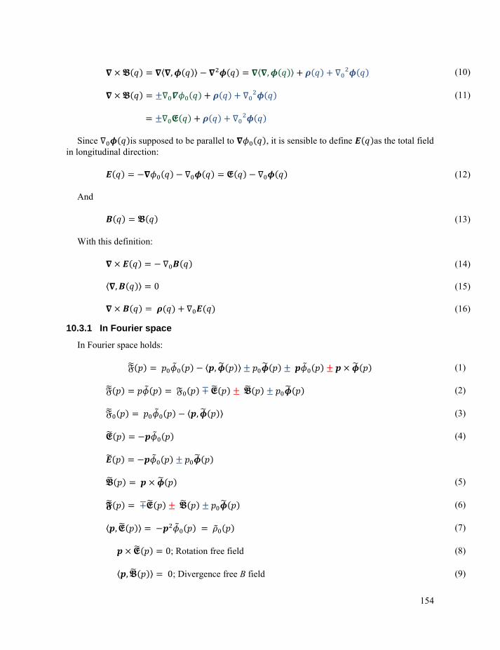
154
⟨ ⟩ ⟨ ⟩
Since is supposed to be parallel to , it is sensible to define as the total field
in longitudinal direction:
And
With this definition:
⟨ ⟩
10.3.1 In Fourier space
In Fourier space holds:
⟨ ⟩
⟨ ⟩
⟨ ⟩
; Rotation free field
⟨ ⟩ ; Divergence free B field
(10)
(11)
(12)
(13)
(14)
(15)
(16)
(1)
(2)
(3)
(4)
(5)
(6)
(7)
(8)
(9)
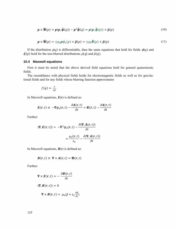
155
⟨ ⟩ ⟨ ⟩
If the distribution (q) is differentiable, then the same equations that hold for fields ϕ(q) and
hold for the non-blurred distributions (q) and .
10.4 Maxwell equations
First it must be noted that the above derived field equations hold for general quaternionic
fields.
The resemblance with physical fields holds for electromagnetic fields as well as for gravita-
tional fields and for any fields whose blurring function approximates
| |.
In Maxwell equations, E(r) is defined as:
≡
Further:
⟨ ⟩ ⟨ ⟩
⟨ ⟩
In Maxwell equations, B(r) is defined as:
≡
Further:
⟨ ⟩
)
(10)
(11)
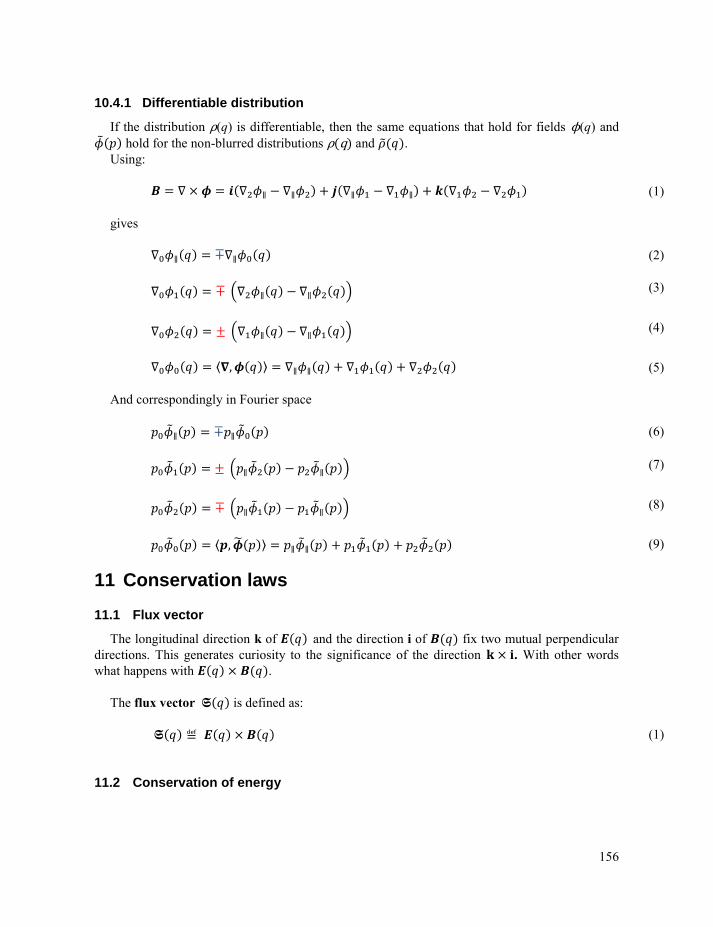
156
10.4.1 Differentiable distribution
If the distribution (q) is differentiable, then the same equations that hold for fields ϕ(q) and
hold for the non-blurred distributions (q) and . Using:
gives
( )
( )
⟨ ⟩
And correspondingly in Fourier space
( )
( )
⟨ ⟩
11 Conservation laws
11.1 Flux vector
The longitudinal direction k of and the direction i of fix two mutual perpendicular
directions. This generates curiosity to the significance of the direction . With other words
what happens with .
The flux vector is defined as:
11.2 Conservation of energy
(1)
(2)
(3)
(4)
(5)
(6)
(7)
(8)
(9)
(1)
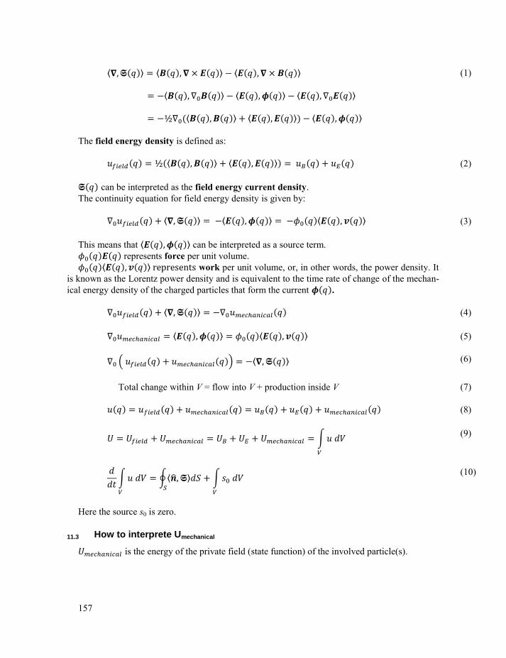
157
⟨ ⟩ ⟨ ⟩ ⟨ ⟩
⟨ ⟩ ⟨ ⟩ ⟨ ⟩
⟨ ⟩ ⟨ ⟩ ⟨ ⟩
The field energy density is defined as:
⟨ ⟩ ⟨ ⟩
can be interpreted as the field energy current density.
The continuity equation for field energy density is given by:
⟨ ⟩ ⟨ ⟩ ⟨ ⟩
This means that ⟨ ⟩ can be interpreted as a source term.
represents force per unit volume.
⟨ ⟩ represents work per unit volume, or, in other words, the power density. It
is known as the Lorentz power density and is equivalent to the time rate of change of the mechan-
ical energy density of the charged particles that form the current .
⟨ ⟩
⟨ ⟩ ⟨ ⟩
( ) ⟨ ⟩
Total change within V = flow into V + production inside V
∫
∫
∮⟨ ⟩
∫
Here the source s0 is zero.
11.3 How to interprete Umechanical
is the energy of the private field (state function) of the involved particle(s).
(1)
(2)
(3)
(4)
(5)
(6)
(7)
(8)
(9)
(10)
158
11.4 Conservation of linear momentum
can also be interpreted as the field linear momentum density. The time rate change of
the field linear momentum density is:
( )
⟨ ⟩ ⟨ ⟩ ⟨ ⟩ ⟨ ⟩
⟨ ⟩ ⟨ ⟩
⟨ ⟩ ⟨ ⟩
⟨ ⟩ ⟨ ⟩
⟨ ⟩
⟨ ⟩ ⟨ ⟩
is the linear momentum flux tensor.
The linear momentum of the field contained in volume V surrounded by surface S is:
∫
∫
∫ ⟨ ⟩ ∮⟨ ⟩
Physically, is the Lorentz force density. It equals the time rate change of the mechanical
linear momentum density .
The force acted upon a single particle that is contained in a volume V is:
∫
∫
Brought together this gives:
(1)
(2)
(3)
(4)
(5)
(6)
(7)
(8)
(9)
(10)
159
( ) ⟨ ⟩
This is the continuity equation for linear momentum.
The component is the linear momentum in the i-th direction that passes a surface element in
the j-th direction per unit time, per unit area.
Total change within V = flow into V + production inside V
∫
∫
∮⟨ ⟩
∫
Here the source sg = 0.
11.5 Conservation of angular momentum
11.5.1 Field angular momentum
The angular momentum relates to the linear momentum.
(q)
This enables the balance equation for angular momentum:
( ) ⟨ ⟩
Total change within V = flow into V + production inside V
∫
(11)
(12)
(13)
(14)
(15)
(1)
(2)
(3)
(4)
(5)
(6)
(7)
160
∫
∮⟨ ⟩
∫
Here the source sh = 0.
For a localized charge density contained within a volume V holds for the mechanical torsion:
∫
∫ ( )
Using
⟨ ⟩
⟨ ⟩
holds
∫
∫
∫ ⟨ ⟩ ⟨ ⟩
∫ ⟨ ⟩
∫
∫⟨ ⟩
∫ ⟨ ⟩
11.5.2 Spin
Define the non-local spin term, which does not depend on qʹ as:
(8)
(9)
(10)
(11)
(12)
161
∫
Notice
( )
And
∫ ⟨ ⟩
∫
Using Gauss:
∫⟨ ⟩
∮⟨ ⟩
And
⟨ ⟩
Leads to:
∮⟨ ⟩
11.5.3 Spin discussion
The spin term is defined by:
∫
In free space the charge density 0 vanishes and the scalar potential ϕ0 shows no variance. Only the vector potential ϕ may vary with q0. Thus:
∫
Depending on the selected field Σfield has two versions that differ in their sign. These ver-sions can be combined in a single operator:
[
]
(13)
(14)
(15)
(16)
(17)
(1)
(2)
(3)
(4)
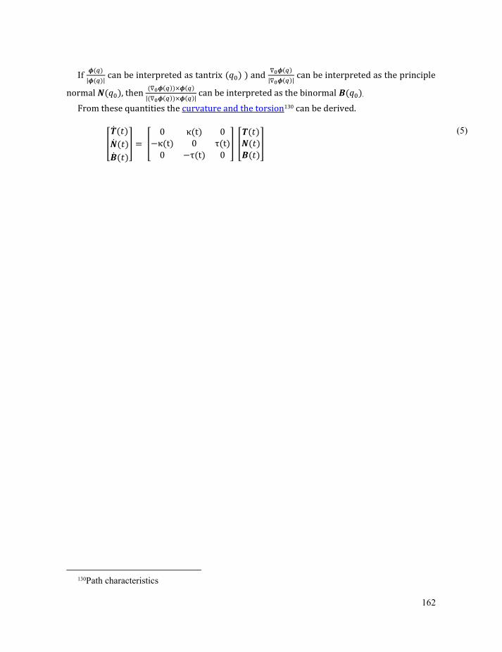
162
If
| | can be interpreted as tantrix ) and
| | can be interpreted as the principle
normal , then
| | can be interpreted as the binormal .
From these quantities the curvature and the torsion130 can be derived.
[
] [
t t t
t ] [
]
130Path characteristics
(5)
163
12 The universe of items
All particles have properties. Some of these properties expose as sources of corresponding
fields. Via superposition these fields interact. Long range fields such as the gravitation field have
universe wide effects.
12.1 Inertia
The influence of items in universe may decrease with distance according to some function of the distance 131. However the number of contributing items increases with the distance. De-
pending on function the most probable result is that the strongest influence comes from the
cooperative activity of the most distant items. Due to the enormous number of items in the uni-
verse, any variation of the influences of the distant items averages away. This also holds for the
density distribution of the items. So there exists a fairly uniform background influence caused by
the universe of items. What will happen, can be deduced from an equivalent of Denis Sciama’s
analysis132133134. We will take his analysis as a guide. Sciama’s analysis uses a different setting: the
(observed) 3D space and coordinate time and Sciama applies Maxwell field theory. We use the
coordinate space defined by an appropriate coordinate operator that resides in the Gelfand triple of
the separable Hilbert space and the progression parameter that relates to the progression step
counter as our setting. A location in this coordinate space represents a location on the unit sphere
of Gelfand triple. This last location is taken by the eigenvector that corresponds to the first loca-
tion.
As stated before, the unit sphere of Gelfand triple is an affine space. This means that we must
treat position as relative data. With other words, the eigenspace of the coordinate operator has no
absolute origin. Instead of Sciama’s usage of Maxwell fields we will use quaternionic field theory
that is applied to quaternionic probability amplitude distributions (QPAD’s).
We may specify a QPAD for usage in a continuity equation. In that case we specify in fact the
combination of a charge density distribution and a current density distribution. As long as the
charges and the currents stay static, the QPAD is a static object.
In the continuity equation we consider the influence of the QPAD on the whole universe. Here
we consider the influence of the universe on a local charge or current. For this purpose we can use
similar QPAD’s and volume integrals!
At large distances, the density of the contributing items can be considered to be uniformly
distributed. Also any variance in strength other than the dependence on becomes negligible be-
cause the differences between functions { } average away. We take the average of the strength
of { } as the significant parameter. We combine it with ρ. Therefore the average of ρ can be
taken out of the integral.
131 http://en.wikipedia.org/wiki/Bertrand's_theorem and Role of the particle locator operator 132 http://arxiv.org/abs/physics/0609026v4.pdf 133 http://www.adsabs.harvard.edu/abs/1953MNRAS.113...34S 134http://rmp.aps.org/abstract/RMP/v36/i1/p463_1
164
The total potential at the location of the influenced subject is135
∫
∫
What we have here is the reverse of the definition of the potential that goes together with a
charge distribution.
The integral is taken over the coordinate space volume . Indirectly, the integral is taken over
the unit sphere of the Gelfand triple. This is an affine space. The parameter is the length of the
vector from the actor to the location of the subject. The considered subject is located somewhere
in the affine coordinate space. All other subjects have positions relative to that considered subject.
Thus, apart from its dependence on the average value of ρ, Φ is a huge constant. Sciama relates Φ
to the gravitational constant .
⁄
As a consequence we can consider the universe as a very large rigid body. If nothing else hap-
pens then all influences compensate each other.
In contrast to Sciama, we use imaginary quaternions rather than 3D vectors. This also avoids
the distracting factor i.
If the considered subject moves relative to the universe with a uniform speed v, then a vector
potential A is generated.
= ∫
Both ρ and v are independent of r. The product represents a current. Together with the con-
stant c they can be taken out of the integral. Thus
A = Φ·v/c
The notions of charge and current correspond to equivalent notions in Noether’s theo-rem136. Here we talk about inertia. Thus charge may symbolize mass. Or even better; it sym-bolizes the coupling factor that plays the role of mass.
The progression parameter t plays the role of “time”. Be aware, in our setting it is the progres-
sion parameter, which is not the usual notion of time.
According to the Helmholtz theorem the field that is derived from the above potential can be
split into a divergence free part and a rotation free part. The Helmholtz decomposition theorem
135 http://en.wikipedia.org/wiki/Newtonian_potential 136 http://en.wikipedia.org/wiki/Noether%27s_theorem
(1)
(2
)
(3
)
165
only concerns the static versions of the derived field. It is related to the fact that the Fourier trans-
form of a vector field can be split in a longitudinal and a transversal version. A corresponding
split of the multi-dimensional Dirac delta function in a longitudinal and a transversal version ex-
ists as well.
According to Maxwell field theory as well as according to quaternionic field theory, a variation
of goes together with a variation of A. On its turn this goes together with a non-zero field
which is a dynamical part of the QPAD. Thus, with varying the QPAD is no longer stat-
ic.137
Sciama uses a Maxwell equation to explain the relation between ∂v/∂t and . Our setting
differs, but the quaternionic field theory delivers the same results.
If we exclude the first term because it is negligible small, we get:
t
t
Remark: As soon as we turn to the dynamic version (4) an extra component of field E ap-
pears that corresponds to acceleration ∂v/∂t.138
As already claimed, in our setting the component of the field E is negligible. With respect
to this component the items compensate each other’s influence. This means that if the influenced
subject moves with uniform speed v, then E ≈ 0. However, a vector potential A is present due to
the movement of the considered item. Like and , and together form a QPAD. Any ac-
celeration of the considered item goes together with an extra non-zero E field. In this way the
universe of items causes inertia in the form of a force that acts upon the accelerating item’s
charge. The item is the carrier of the charge .
The situation in curved space differs. When the path of the item coincides with a geodesic,
then it can be travelled free of extra generated fields. Thus, a uniform movement along the geo-
desic does not on itself generate a reaction of the universe of items. Any alteration of that uniform
movement will go together with the existence of an extra field. The physical name for this reac-
tion is action. It usually gets the symbol S.
On the other hand, as we see from inertia, any field change goes together with a corresponding
acceleration. Uniform movements do cause displacement of charges. In a curved environment it
137 See Differentiation 138 See http://www.plasma.uu.se/CED/Book; formula 3.25 or Appendix; Maxwell equations
(4)
(5)
(6)
166
changes the configuration of the QPAD. Thus, in that case, even an originally static QPAD may
be affected.
We may reverse the conclusion of the analysis:
An extra field component goes together with an acceleration of the local item.
The acceleration can be seen as the consequence of a local curvature and vice versa. Thus, the
extra field goes together with a local curvature.
It must be noticed that the original analysis of Sciama uses observable position space rather
coordinate space and it uses a different notion of time. However, the general conclusion stays the
same. Sciama’s analysis is criticized because it uses infinite speed of information transfer. Since
we do not work in observable position space, we do not encounter coordinate time. So for the set-
ting of our analysis, this criticism is misplaced. Most part of the story plays in a stationary QPAD
condition. As long as the movement stays uniform, the QPAD is static. Any acceleration deviates
from this stationary condition. This deviation goes together with an extra field component and it
goes together with a local curvature.
Coordinate time139 relates to observations of position. It is a local player in the game, where the
progression parameter is a global player.
The situation with electromagnetic fields is different, because with this field positive and nega-
tive charges compensate each other’s long range influence. For that reason there exists no elec-
tromagnetic background influence. The masses of the gravitational and inertial fields only com-
pensate each other’s long range influences through geometrical circumstances. Still in
combination, they create gigantic potentials.
The particles outside the information horizons also contribute to the inertia.
Thus when through uniform movement the local field configuration changes, then that change
goes together with an acceleration of the local item.
12.2 Nearby items
Items that are located nearby have a different effect. In general their influence will not have its
strength equal to the average strength. Further these items are not uniformly distributed. Still at
macroscopic distances their influence depends on inter-distance as . As a consequence
their influences form a landscape of which the effects will become sensible in the action of the
fields that surround the considered item. For observers, this landscape will form a curved action
space. The considered item will try to follow a geodesic through that curved space.
12.3 Rotational inertia
Besides linear inertia there exists rotational inertia. In a non-rotating universe hold near the
origin A = 0 and Φ = -c2/G. We choose units such that c=G=1. In a universe rotating slowly with
angular speed ω hold
139 Dynamics; Relativity
167
Ax = ω·y
Ay = ω·x
Az = 0
√
A constant angular movement meets the fields that correspond to a centripetal force.
The field E has the form
√
An added uniform speed v meets the fields corresponding to a Coriolis force.
The forces are usually considered as fictitious but they are actually caused by inertia. Sciama
treats them in section 5 of his paper. Like fields of linear inertia these rotation related fields corre-
spond to actions of the manipulator.
12.4 Computation of the background QPAD
The same line of thinking that lead to the formula for the local potential in section 12.1-(1) can
be applied to the computation of the QPAD that represents the local background field.
The ensemble { ψ } is distributed randomly over the center points { } in an affine pa-
rameter space. At a given point P in this space the superposition of all { ψ } will be con-
structed.
This superposition will be renormalized and then indicated by Φ . Thus,
∫|Φ |
In this superposition the largest contribution comes from the ψ for which the is far-
thest from P. Further the directions of the imaginary part of Φ .are reversed with respect to
the directions in the ψ . Especially at long distances, all differences are smoothed away via an averaging process.
The result is that for the average QPAD :
(1)
(2)
(3)
(4)
(5)
(6)
(7)
(1)
168
Φ =
We will interpret Φ as the background QPAD.
Since we are talking about quaternionic distributions it is possible that every sign flavor has its
own background QPAD.
13 Path characteristics
The Frenet-Serret frame is devised for describing curved paths of particles
Let {αqt}t = α(q,t) describe a curved path consisting of infinitesimal steps through a landscape
{αq}q = α(q) of imaginary quaternions αqt, such that || || for all t.
The 3D Frenet-Serret frame for the above path is given by:
( ) ( )
|| ||
|| || || || || ||
is the tantrix of curve α(q(t)) at instance t.
is the principal normal of curve α(q(t)) at instance t. It is only defined when κ(t) ≠ 0.
is the binormal of curve α(q(t)) at instance t.
, and are imaginary quaternions.
κ(t) is the curvature of curve at α(q(t)) at instance t.
r(t) = 1/ κ(t) is the radius of curvature at instance t.
τ(t) is the torsion of curve α(q(t)) at instance t.
[
] [
t t t
t ] [
]
The Frenet-Serret curves have particular characteristics. The path may be curved and curled.
The path is completely determined by its tantrix, curvature and torsion given by functions of t.
Each coordinate of the quaternionic function α(q(t)) has its own set of characteristics. This means
that for a given quaternionic function these characteristics are quaternions rather than real num-
bers and they are all functions of parameter t.
(2)
(1
)
(2
)
(3
)
(4
)
(5
)
(6
)
169
13.1 Path equations
The path equations are given by
t
t t t t
t
t
13.2 Curve length
The curve length is defined by:
∫ | |
The integration over the square of the modulus delivers the action S of the curve.
∫ | |
13.3 Reparameterization
The path characteristics κ(t) and τ(t) together with the curve length and the curve action are in-
dependent of any reparameterization of the progression parameter t.
A natural reparameterization is given by .
This turns the curve t into a natural curve ( s ):
( s ) t
Curves on a surface which minimize length between the endpoints are called geodesics.
The natural curve corresponds to a geodesic140.
The consequence is that in three-dimensional space the corresponding movement obeys the ge-
odesic equation141. The Lagrangian is an equivalent of this equation.
140 http://en.wikipedia.org/wiki/Geodesic 141 Equations of motion; Lagrangian
(1)
(2)
(3)
(1)
(2)
(1)
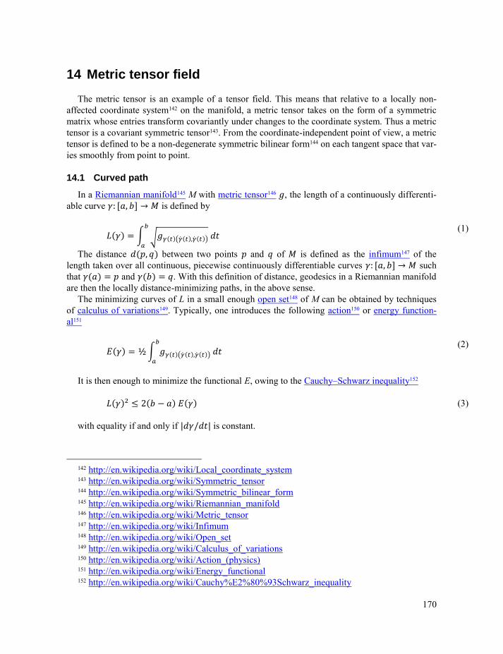
170
14 Metric tensor field
The metric tensor is an example of a tensor field. This means that relative to a locally non-
affected coordinate system142 on the manifold, a metric tensor takes on the form of a symmetric
matrix whose entries transform covariantly under changes to the coordinate system. Thus a metric
tensor is a covariant symmetric tensor143. From the coordinate-independent point of view, a metric
tensor is defined to be a non-degenerate symmetric bilinear form144 on each tangent space that var-
ies smoothly from point to point.
14.1 Curved path
In a Riemannian manifold145 M with metric tensor146 , the length of a continuously differenti-
able curve : [ ] is defined by
∫ √ ( )
The distance between two points and of is defined as the infimum147 of the
length taken over all continuous, piecewise continuously differentiable curves : [ ] such
that and . With this definition of distance, geodesics in a Riemannian manifold
are then the locally distance-minimizing paths, in the above sense.
The minimizing curves of L in a small enough open set148 of M can be obtained by techniques
of calculus of variations149. Typically, one introduces the following action150 or energy function-
al151
∫ ( )
It is then enough to minimize the functional E, owing to the Cauchy–Schwarz inequality152
with equality if and only if | | is constant.
142 http://en.wikipedia.org/wiki/Local_coordinate_system 143 http://en.wikipedia.org/wiki/Symmetric_tensor 144 http://en.wikipedia.org/wiki/Symmetric_bilinear_form 145 http://en.wikipedia.org/wiki/Riemannian_manifold 146 http://en.wikipedia.org/wiki/Metric_tensor 147 http://en.wikipedia.org/wiki/Infimum 148 http://en.wikipedia.org/wiki/Open_set 149 http://en.wikipedia.org/wiki/Calculus_of_variations 150 http://en.wikipedia.org/wiki/Action_(physics) 151 http://en.wikipedia.org/wiki/Energy_functional 152 http://en.wikipedia.org/wiki/Cauchy%E2%80%93Schwarz_inequality
(1)
(2)
(3)
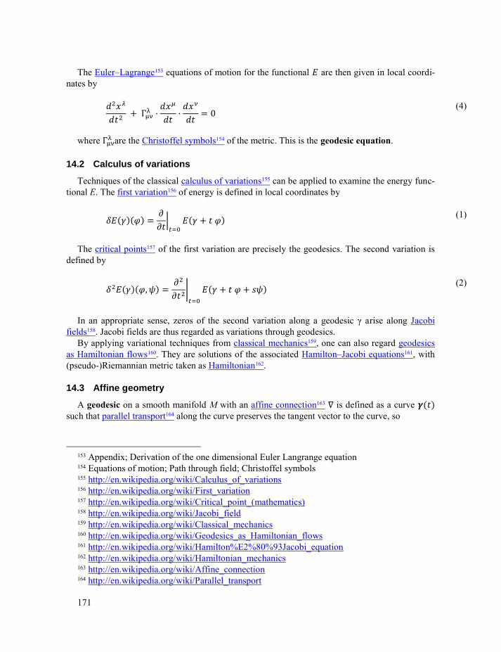
171
The Euler–Lagrange153 equations of motion for the functional are then given in local coordi-
nates by
where are the Christoffel symbols154 of the metric. This is the geodesic equation.
14.2 Calculus of variations
Techniques of the classical calculus of variations155 can be applied to examine the energy func-
tional E. The first variation156 of energy is defined in local coordinates by
|
The critical points157 of the first variation are precisely the geodesics. The second variation is
defined by
|
In an appropriate sense, zeros of the second variation along a geodesic γ arise along Jacobi
fields158. Jacobi fields are thus regarded as variations through geodesics.
By applying variational techniques from classical mechanics159, one can also regard geodesics
as Hamiltonian flows160. They are solutions of the associated Hamilton–Jacobi equations161, with
(pseudo-)Riemannian metric taken as Hamiltonian162.
14.3 Affine geometry
A geodesic on a smooth manifold M with an affine connection163 is defined as a curve such that parallel transport164 along the curve preserves the tangent vector to the curve, so
153 Appendix; Derivation of the one dimensional Euler Langrange equation 154 Equations of motion; Path through field; Christoffel symbols 155 http://en.wikipedia.org/wiki/Calculus_of_variations 156 http://en.wikipedia.org/wiki/First_variation 157 http://en.wikipedia.org/wiki/Critical_point_(mathematics) 158 http://en.wikipedia.org/wiki/Jacobi_field 159 http://en.wikipedia.org/wiki/Classical_mechanics 160 http://en.wikipedia.org/wiki/Geodesics_as_Hamiltonian_flows 161 http://en.wikipedia.org/wiki/Hamilton%E2%80%93Jacobi_equation 162 http://en.wikipedia.org/wiki/Hamiltonian_mechanics 163 http://en.wikipedia.org/wiki/Affine_connection 164 http://en.wikipedia.org/wiki/Parallel_transport
(4)
(1)
(2)
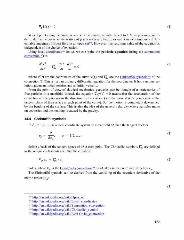
172
at each point along the curve, where is the derivative with respect to t. More precisely, in or-
der to define the covariant derivative of it is necessary first to extend to a continuously differ-
entiable imaginary Hilbert field in an open set165. However, the resulting value of the equation is
independent of the choice of extension.
Using local coordinates166 on M, we can write the geodesic equation (using the summation
convention167) as
where xμ(t) are the coordinates of the curve and
are the Christoffel symbols168 of the
connection . This is just an ordinary differential equation for the coordinates. It has a unique so-
lution, given an initial position and an initial velocity.
From the point of view of classical mechanics, geodesics can be thought of as trajectories of
free particles in a manifold. Indeed, the equation means that the acceleration of the
curve has no components in the direction of the surface (and therefore it is perpendicular to the
tangent plane of the surface at each point of the curve). So, the motion is completely determined
by the bending of the surface. This is also the idea of the general relativity where particles move
on geodesics and the bending is caused by the gravity.
14.4 Christoffel symbols
If xi, i = 1,2,...,n, is a local coordinate system on a manifold M, then the tangent vectors
define a basis of the tangent space of M at each point. The Christoffel symbols are defined
as the unique coefficients such that the equation
holds, where is the Levi-Civita connection169 on M taken in the coordinate direction .
The Christoffel symbols can be derived from the vanishing of the covariant derivative of the
metric tensor gik:
165 http://en.wikipedia.org/wiki/Open_set 166 http://en.wikipedia.org/wiki/Local_coordinates 167 http://en.wikipedia.org/wiki/Summation_convention 168 http://en.wikipedia.org/wiki/Christoffel_symbol 169 http://en.wikipedia.org/wiki/Levi-Civita_connection
(1)
(2)
(1)
(2)
(3)
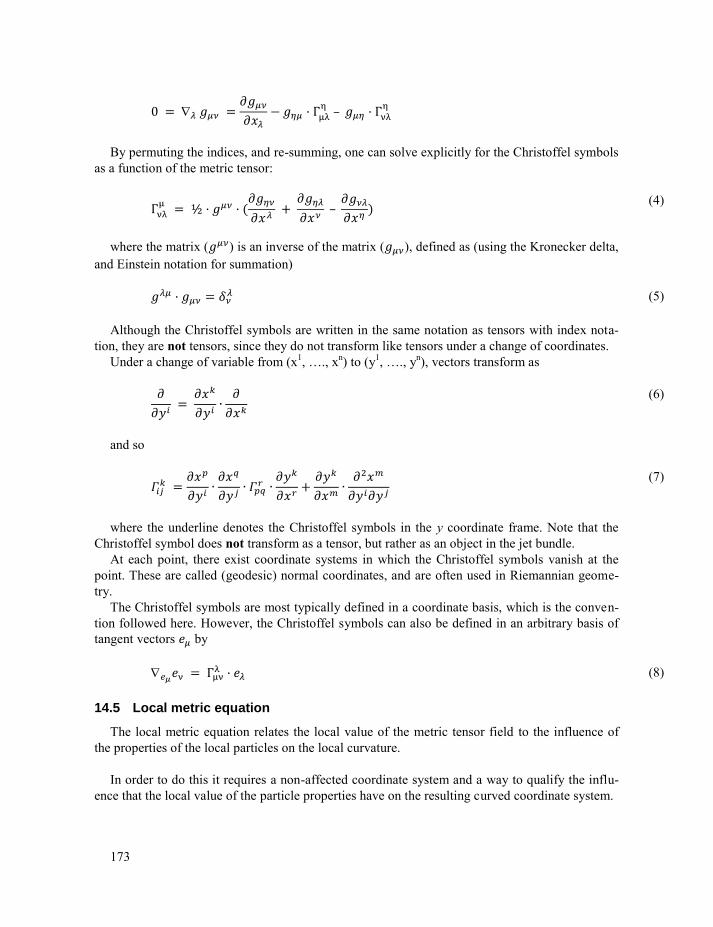
173
By permuting the indices, and re-summing, one can solve explicitly for the Christoffel symbols
as a function of the metric tensor:
where the matrix ( ) is an inverse of the matrix ( ), defined as (using the Kronecker delta,
and Einstein notation for summation)
Although the Christoffel symbols are written in the same notation as tensors with index nota-
tion, they are not tensors, since they do not transform like tensors under a change of coordinates.
Under a change of variable from (x1, …., x
n) to (y
1, …., y
n), vectors transform as
and so
where the underline denotes the Christoffel symbols in the y coordinate frame. Note that the
Christoffel symbol does not transform as a tensor, but rather as an object in the jet bundle.
At each point, there exist coordinate systems in which the Christoffel symbols vanish at the
point. These are called (geodesic) normal coordinates, and are often used in Riemannian geome-
try.
The Christoffel symbols are most typically defined in a coordinate basis, which is the conven-
tion followed here. However, the Christoffel symbols can also be defined in an arbitrary basis of
tangent vectors by
14.5 Local metric equation
The local metric equation relates the local value of the metric tensor field to the influence of
the properties of the local particles on the local curvature.
In order to do this it requires a non-affected coordinate system and a way to qualify the influ-
ence that the local value of the particle properties have on the resulting curved coordinate system.
(4)
(5)
(6)
(7)
(8)
174
For example the Kerr Newman metric equation uses the per category summed property values
of the local coupling factors, the electric charges of the local particles and the angular momenta of
the local particles in order to relate these to the local curvature170.
14.5.1 Kerr-Newman metric equation
The Kerr–Newman metric equation describes the geometry of spacetime in the vicinity of a ro-
tating mass M with charge Q. The formula for this metric depends upon what coordinates or coor-
dinate conditions are selected.
It uses three local properties. These properties are:
The coupling factor
The electric charge
The angular momentum
The angular momentum includes the spin .
In most cases, the simplest interpretation of the Kerr-Newman metric can be taken on the sur-
face of a sphere that has a selected radius . This metric uses the sum of a category of properties
that are collected within the observed sphere. However, the summation produces different centers
of activity for different property categories. Thus, these centers need not be at the same location.
However, for large enough selected radius and applied to black holes or single particles, these
centers coincide.
The formula uses three characteristic radii, whose prominence usually differs with the content
of the investigated sphere.
The metric uses a non-curved coordinate system to start with. Several coordinate systems can
be used. The most common coordinate systems for a non-curved three dimensional space are:
Cartesian coordinates
Spherical coordinates
Alternatives for spherical coordinates are:
Schwarzschild coordinates171
Kruskal-Szekeres coordinates172
Lemaitre coordinates173
Eddington–Finkelstein coordinates174
170 See next part. 171 http://en.wikipedia.org/wiki/Schwarzschild_coordinates 172 http://en.wikipedia.org/wiki/Kruskal-Szekeres_coordinates 173 http://en.wikipedia.org/wiki/Lemaitre_coordinates 174 http://en.wikipedia.org/wiki/Eddington%E2%80%93Finkelstein_coordinates
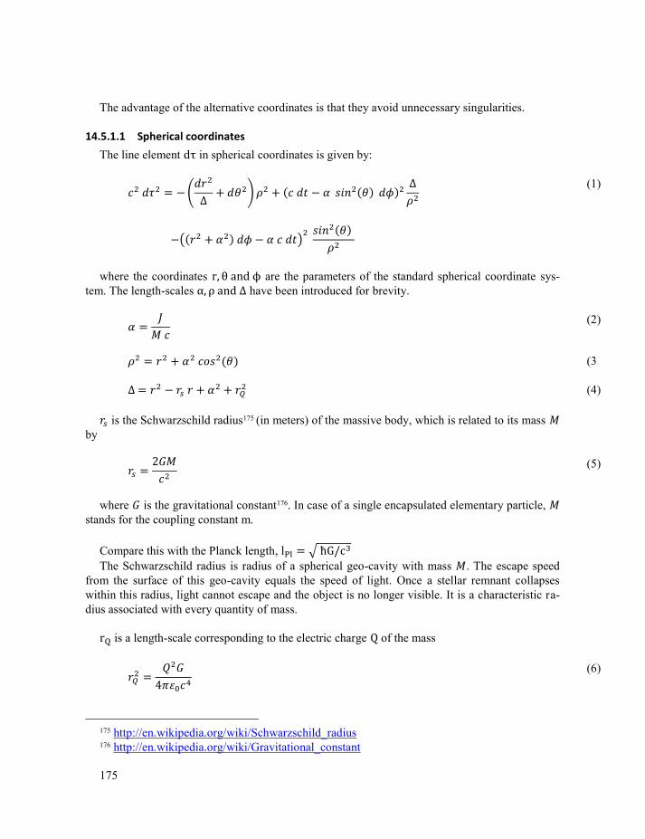
175
The advantage of the alternative coordinates is that they avoid unnecessary singularities.
14.5.1.1 Spherical coordinates
The line element d in spherical coordinates is given by:
(
)
( )
where the coordinates r and ϕ are the parameters of the standard spherical coordinate sys-
tem. The length-scales α and have been introduced for brevity.
is the Schwarzschild radius175 (in meters) of the massive body, which is related to its mass
by
where is the gravitational constant176. In case of a single encapsulated elementary particle,
stands for the coupling constant m.
Compare this with the Planck length, l √ c
The Schwarzschild radius is radius of a spherical geo-cavity with mass . The escape speed
from the surface of this geo-cavity equals the speed of light. Once a stellar remnant collapses
within this radius, light cannot escape and the object is no longer visible. It is a characteristic ra-
dius associated with every quantity of mass.
r is a length-scale corresponding to the electric charge Q of the mass
175 http://en.wikipedia.org/wiki/Schwarzschild_radius 176 http://en.wikipedia.org/wiki/Gravitational_constant
(1)
(2)
(3
(4)
(5)
(6)
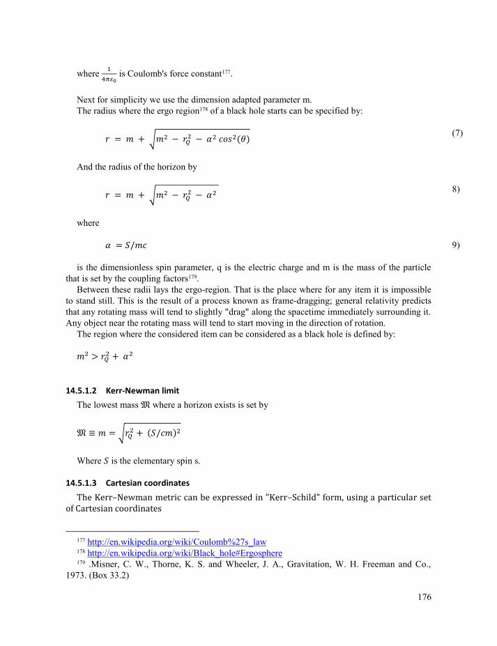
176
where
is Coulomb's force constant177.
Next for simplicity we use the dimension adapted parameter m.
The radius where the ergo region178 of a black hole starts can be specified by:
√
And the radius of the horizon by
√
where
is the dimensionless spin parameter, q is the electric charge and m is the mass of the particle
that is set by the coupling factors179.
Between these radii lays the ergo-region. That is the place where for any item it is impossible
to stand still. This is the result of a process known as frame-dragging; general relativity predicts
that any rotating mass will tend to slightly "drag" along the spacetime immediately surrounding it.
Any object near the rotating mass will tend to start moving in the direction of rotation.
The region where the considered item can be considered as a black hole is defined by:
14.5.1.2 Kerr-Newman limit
The lowest mass 𝔐 where a horizon exists is set by
𝔐 ≡ √
Where is the elementary spin s.
14.5.1.3 Cartesian coordinates
The Kerr Newman metric can be expressed in "Kerr Schild" form, using a particular set of Cartesian coordinates
177 http://en.wikipedia.org/wiki/Coulomb%27s_law 178 http://en.wikipedia.org/wiki/Black_hole#Ergosphere 179 .Misner, C. W., Thorne, K. S. and Wheeler, J. A., Gravitation, W. H. Freeman and Co.,
1973. (Box 33.2)
(7)
8)
9)
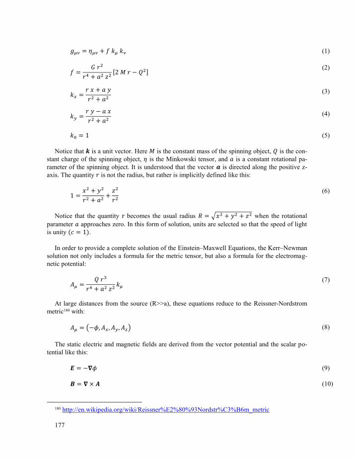
177
[ ]
Notice that is a unit vector. Here is the constant mass of the spinning object, is the con-
stant charge of the spinning object, is the Minkowski tensor, and is a constant rotational pa-
rameter of the spinning object. It is understood that the vector is directed along the positive z-
axis. The quantity is not the radius, but rather is implicitly defined like this:
Notice that the quantity r becomes the usual radius √ when the rotational
parameter approaches zero. In this form of solution, units are selected so that the speed of light
is unity .
In order to provide a complete solution of the Einstein–Maxwell Equations, the Kerr–Newman
solution not only includes a formula for the metric tensor, but also a formula for the electromag-
netic potential:
At large distances from the source (R>>a), these equations reduce to the Reissner-Nordstrom
metric180 with:
( )
The static electric and magnetic fields are derived from the vector potential and the scalar po-
tential like this:
180 http://en.wikipedia.org/wiki/Reissner%E2%80%93Nordstr%C3%B6m_metric
(1)
(2)
(3)
(4)
(5)
(6)
(7)
(8)
(9)
(10)
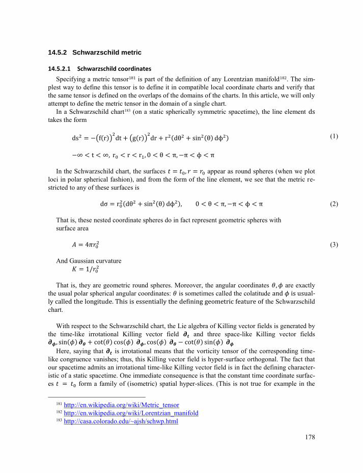
178
14.5.2 Schwarzschild metric
14.5.2.1 Schwarzschild coordinates
Specifying a metric tensor181 is part of the definition of any Lorentzian manifold182. The sim-
plest way to define this tensor is to define it in compatible local coordinate charts and verify that
the same tensor is defined on the overlaps of the domains of the charts. In this article, we will only
attempt to define the metric tensor in the domain of a single chart.
In a Schwarzschild chart183 (on a static spherically symmetric spacetime), the line element ds takes the form
ds (f r ) dt (g r )
dr r d sin dϕ
t r r r ϕ
In the Schwarzschild chart, the surfaces appear as round spheres (when we plot
loci in polar spherical fashion), and from the form of the line element, we see that the metric re-
stricted to any of these surfaces is
d r d sin dϕ ϕ
That is, these nested coordinate spheres do in fact represent geometric spheres with
surface area
And Gaussian curvature
That is, they are geometric round spheres. Moreover, the angular coordinates are exactly
the usual polar spherical angular coordinates: is sometimes called the colatitude and is usual-ly called the longitude. This is essentially the defining geometric feature of the Schwarzschild
chart.
With respect to the Schwarzschild chart, the Lie algebra of Killing vector fields is generated by
the time-like irrotational Killing vector field and three space-like Killing vector fields
sin cot cos cos cot sin
Here, saying that is irrotational means that the vorticity tensor of the corresponding time-
like congruence vanishes; thus, this Killing vector field is hyper-surface orthogonal. The fact that
our spacetime admits an irrotational time-like Killing vector field is in fact the defining character-
istic of a static spacetime. One immediate consequence is that the constant time coordinate surfac-
es form a family of (isometric) spatial hyper-slices. (This is not true for example in the
181 http://en.wikipedia.org/wiki/Metric_tensor 182 http://en.wikipedia.org/wiki/Lorentzian_manifold 183 http://casa.colorado.edu/~ajsh/schwp.html
(1)
(2)
(3)
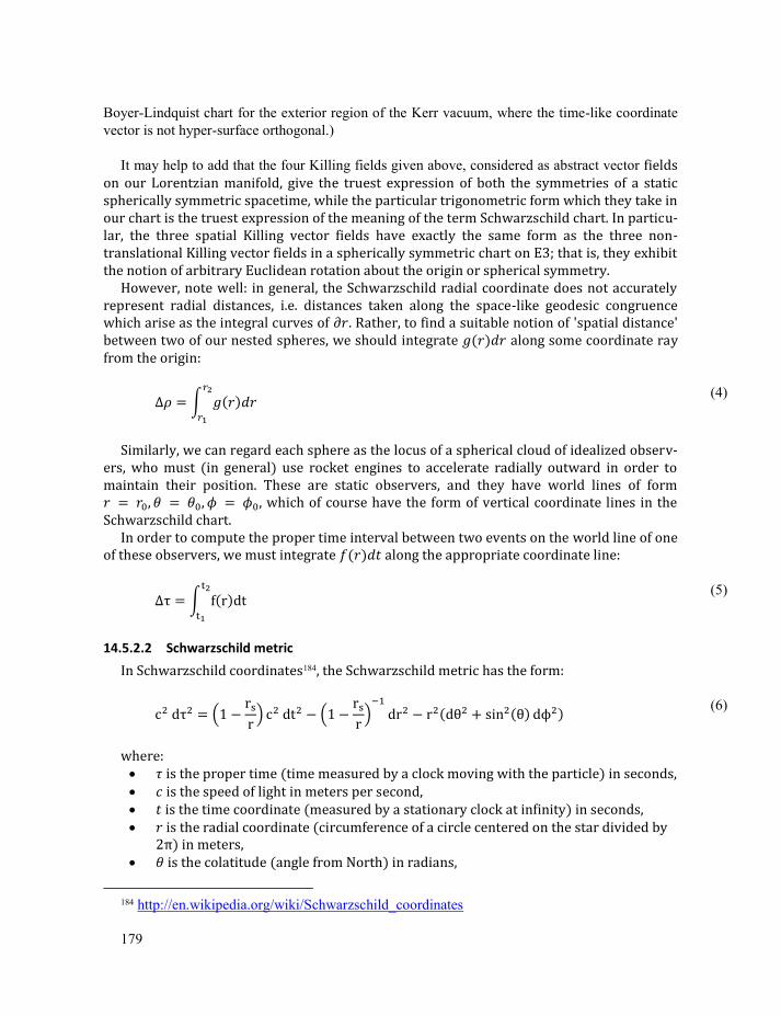
179
Boyer-Lindquist chart for the exterior region of the Kerr vacuum, where the time-like coordinate
vector is not hyper-surface orthogonal.)
It may help to add that the four Killing fields given above, considered as abstract vector fields on our Lorentzian manifold, give the truest expression of both the symmetries of a static spherically symmetric spacetime, while the particular trigonometric form which they take in our chart is the truest expression of the meaning of the term Schwarzschild chart. In particu-lar, the three spatial Killing vector fields have exactly the same form as the three non-translational Killing vector fields in a spherically symmetric chart on E3; that is, they exhibit the notion of arbitrary Euclidean rotation about the origin or spherical symmetry.
However, note well: in general, the Schwarzschild radial coordinate does not accurately represent radial distances, i.e. distances taken along the space-like geodesic congruence which arise as the integral curves of . Rather, to find a suitable notion of 'spatial distance' between two of our nested spheres, we should integrate along some coordinate ray from the origin:
∫
Similarly, we can regard each sphere as the locus of a spherical cloud of idealized observ-
ers, who must (in general) use rocket engines to accelerate radially outward in order to maintain their position. These are static observers, and they have world lines of form , which of course have the form of vertical coordinate lines in the Schwarzschild chart.
In order to compute the proper time interval between two events on the world line of one of these observers, we must integrate along the appropriate coordinate line:
∫ f r dt
14.5.2.2 Schwarzschild metric
In Schwarzschild coordinates184, the Schwarzschild metric has the form:
c d ( r r) c dt (
r r)
dr r d sin dϕ
where: is the proper time (time measured by a clock moving with the particle) in seconds, is the speed of light in meters per second, is the time coordinate (measured by a stationary clock at infinity) in seconds, is the radial coordinate (circumference of a circle centered on the star divided by in meters
is the colatitude (angle from North) in radians,
184 http://en.wikipedia.org/wiki/Schwarzschild_coordinates
(4)
(5)
(6)
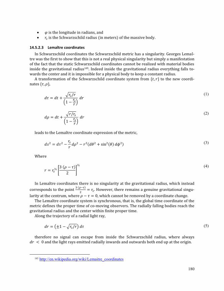
180
is the longitude in radians, and is the Schwarzschild radius (in meters) of the massive body.
14.5.2.3 Lemaître coordinates
In Schwarzschild coordinates the Schwarzschild metric has a singularity. Georges Lemaî-tre was the first to show that this is not a real physical singularity but simply a manifestation of the fact that the static Schwarzschild coordinates cannot be realized with material bodies inside the gravitational radius185. Indeed inside the gravitational radius everything falls to-wards the center and it is impossible for a physical body to keep a constant radius.
A transformation of the Schwarzschild coordinate system from { } to the new coordi-nates { },
√
( )
√
( )
leads to the Lemaître coordinate expression of the metric,
sin
Where
[
]
In Lemaître coordinates there is no singularity at the gravitational radius, which instead
corresponds to the point
. However, there remains a genuine gravitational singu-
larity at the centrum, where , which cannot be removed by a coordinate change. The Lemaître coordinate system is synchronous, that is, the global time coordinate of the
metric defines the proper time of co-moving observers. The radially falling bodies reach the gravitational radius and the center within finite proper time.
Along the trajectory of a radial light ray,
( √ )
therefore no signal can escape from inside the Schwarzschild radius, where always and the light rays emitted radially inwards and outwards both end up at the origin.
185 http://en.wikipedia.org/wiki/Lemaitre_coordinates
(1)
(2)
(3)
(4)
(5)
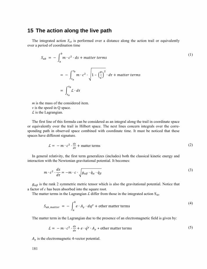
181
15 The action along the live path
The integrated action Sab is performed over a distance along the action trail or equivalently
over a period of coordination time
∫
∫ √ (
)
∫
m is the mass of the considered item.
v is the speed in Q space.
is the Lagrangian.
The first line of this formula can be considered as an integral along the trail in coordinate space
or equivalently over the trail in Hilbert space. The next lines concern integrals over the corre-
sponding path in observed space combined with coordinate time. It must be noticed that these
spaces have different signature.
+ matter terms
In general relativity, the first term generalizes (includes) both the classical kinetic energy and
interaction with the Newtonian gravitational potential. It becomes:
√
is the rank 2 symmetric metric tensor which is also the gravitational potential. Notice that
a factor of c has been absorbed into the square root.
The matter terms in the Lagrangian differ from those in the integrated action Sab.
∫
other matter terms
The matter term in the Lagrangian due to the presence of an electromagnetic field is given by:
+ other matter terms
is the electromagnetic 4-vector potential.
(1)
(2)
(3)
(4)
(5)
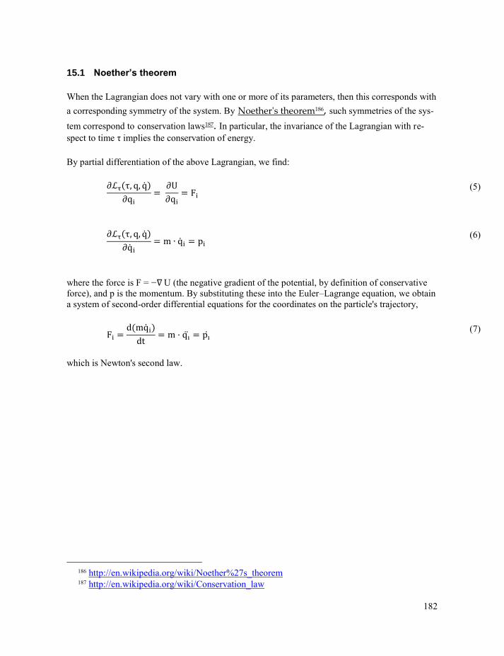
182
15.1 Noether’s theorem
When the Lagrangian does not vary with one or more of its parameters, then this corresponds with
a corresponding symmetry of the system. By Noether's theorem186, such symmetries of the sys-
tem correspond to conservation laws187. In particular, the invariance of the Lagrangian with re-
spect to time τ implies the conservation of energy.
By partial differentiation of the above Lagrangian, we find:
F
m p
where the force is F = − U (the negative gradient of the potential, by definition of conservative
force), and p is the momentum. By substituting these into the Euler–Lagrange equation, we obtain
a system of second-order differential equations for the coordinates on the particle's trajectory,
F d m
dt m p
which is Newton's second law.
186 http://en.wikipedia.org/wiki/Noether%27s_theorem 187 http://en.wikipedia.org/wiki/Conservation_law
(5)
(6)
(7)
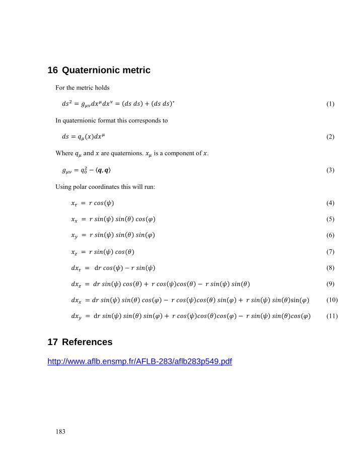
183
16 Quaternionic metric
For the metric holds
In quaternionic format this corresponds to
Where and are quaternions. is a component of .
⟨ ⟩
Using polar coordinates this will run:
d
sin
d
17 References
http://www.aflb.ensmp.fr/AFLB-283/aflb283p549.pdf
(1)
(2)
(3)
(4)
(5)
(6)
(7)
(8)
(9)
(10)
(11)
184
HvL

185

186
187
INDEX
2
n-on construction, 44, 100
2n-ons, 100
3 sphere, 110
action, 165
action along the live path, 181
affine geometry, 171
amplitude distribution
probability amplitude distribution, 20
anisotropic, 45
antiparticle, 54, 63
background
anisotropic backgrounds, 62
background continuum, 37
background field, 42, 56, 59
background QPAD, 42
general background QPAD, 62
isotropic background QPAD, 62
balance equation, 51
base transforms, 133
bi-quaternions, 44
birth of the universe
requirements for the birth of the universe, 84
Birth of the universe, 83
black hole
classical black hole, 79
general black hole, 80
quantum black hole, 80
boson, 62
W boson, 63
Z boson, 63
calculus of variations, 171
canonical conjugate, 37
carrier, 46
virtual carrier, 76
categories of physical fields, 32
Cayley-Dickson construction, 44
Chandrasekhar limit, 82
charge
charge carrier, 46
color charge, 59, 62
electric charge, 62
Christoffel symbols, 172
classical logic, 19
Clifford algebra, 33
coherent state, 131
color charge, 32
colored signs, 48
complex number oriented physics, 24
composite, 62
compression region, 24
conjugation, 26, 44, 48, 51
conservation laws, 156, 182
conservation of angular momentum, 159
conservation of energy, 156
conservation of linear momentum, 158
contemporary physics, 34
continuity equation, 25, 50, 115, 150
continuity equation for field energy density, 157
coordinate
canonical conjugate coordinate, 48
coordinate system
curved coordinate system, 46
flat coordinate system, 46
coordinates
quaternion coordinates, 109
coordinates
polar coordinates, 109
coupled, 42
coupling factor, 31, 54, 55, 57, 58, 59
covariant derivation, 76
CPAD, 25, 48, 52
curvature, 30, 34, 37, 42
space curvature, 29
decompression region, 24
density distribution
charge density distribution, 25, 46, 50
current density distribution, 25, 46, 50
presence probability density distribution, 46
probability density distribution, 50
differentiable distribution, 156
differential potential equations, 153
differentiation, 47
Dirac basis, 49
Dirac delta function
multi-dimensional, 118
Dirac equation, 55, 57
discrete distribution, 153
division ring, 19, 44
down quark, 58
drain, 29
eigenspace, 37
eigenvalue, 37
eigenvector, 37
electric charge, 32
electron, 55
elementary boson, 42
elementary coupling
elementary coupling equation, 31, 54
restricted elementary coupling, 54
elementary coupling equation
restricted elementary coupling equation, 42
elementary fermion, 42
188
elementary particle type, 61
ensemble of properties, 46
equation for the differentiation, 50
equation of motion, 25
eth, 148
fermion, 62
elementary fermion, 62
field angular momentum, 159
field energy current density, 157
field linear momentum
field linear momentum density, 158
field linear momentum flux tensor, 158
first level coupling, 54
first level particle, 54
flip, 58
reverse flip, 56
fluid dynamics, 24
quantum fluid dynamics, 31
flux, 50
flux vector, 156
Fourier space, 48
Fourier transform, 37
alternative approach, 120
alternative definition, 122
convolution, 128
differentiation, 128
Fourier transform equivalents, 55
Fourier transform properties, 127
functions invariant under Fourier transform, 122
invariant under Fourier transform, 38
Fourier transform invariant, 127
Fourier transform of a black hole, 142
Fourier transform split, 118
free moving, 55
free QPAD, 60
funnel, 37
gamma matrices, 49
gauge transform, 152
Gauss theorem, 50
Gaussian distribution, 42
Gelfand triple, 37, 42
general relativity, 172, 181
generations, 32
geodesic, 165, 169
geodesic equation, 169
geodesic equation, 171
Grassmann algebra, 33
ground state, 61, 130
group structure, 111
half ordered set, 95
Hamilton
Sir William Rowan Hamilton, 33
Hamiltonian, 55
handedness, 45, 51, 56, 58, 62, 63
harmonic, 61
harmonic functions
spin-weighted harmonic functions, 148
HBM, 19
HBM page, 21
Heisenberg
Heisenberg picture, 33
Heisenberg picture, 22, 37, 52
Helmholtz decomposition, 38, 164
hidden particles, 64
Higgs field, 42
Hilbert Book Model, 22
Hilbert space, 33
separable Hilbert space, 19, 33, 42
history, 33
history of quantum logic, 95
holographic principle, 81
Hopf coordinates, 111
hyper-complex number, 19
inertia, 153, 163
rotational inertia, 166
Inertia, 41
infinitesimal number transformation, 108
interaction, 76
isotropic, 41, 44
John von Neumann, 33
Jordan algebra, 33
Kerr Newman metric, 174
Kerr–Newman metric
Kerr–Newman metric equation, 174
Lagrangian, 55, 169
lattice, 95
atomic lattice, 97
complementary lattice, 96
distributive lattice, 97
lattice isomorphic, 19
modular lattice, 97
orthocomplemented lattice, 96
weak modular lattice, 97
length contraction, 34
location operator
particle location operator, 51
wave location operator, 51
logic
classical logic, 19, 98
predicate logic, 98
propositional logic, 98
traditional quantum logic, 19, 98
Lorentz force density, 158
Lorentz power density, 157
Lorentz transformation, 34
Majorana equation, 57
mathemagician, 28
matrices, 104
alpha-, beta- and gamma-matrices, 33
matrix, 48, 55
189
Maxwell equations, 155
measurement, 99
metric
Kerr-Newman metric, 89
local metric equation, 89, 173
metric tensor, 170
Minkowski signature, 34
modularization, 78
modulus, 46
momentum, 55
nearby items, 166
neutrino, 58
niners, 102
Noether’s theorem, 164
Noether's theorem, 182
norm, 46
number, 99
construction, 99
hyper-complex number, 44
number waltz, 106
observable, 99
operator
location operator, 42
particle location operator, 42
particle locator operator, 37
position operator, 37
operators
ladder operator, 128
orbital angular momentum, 144
page counter, 22
Palestra, 30, 70
parameter space, 46, 57
non-curved parameter space, 48
shared parameter space, 30
Parseval’s theorem, 127
particle
virtual particle, 27
particle generation, 54
particles
virtual particles, 76
path
curve length, 169
path characteristics, 168
path equations, 169
reparameterization, 169
Pauli matrices, 48
physical field, 34
first category physical field, 41, 82
second category physical field, 26, 41, 43, 73,
75, 82, 83, 116
physical reality, 24
Piron
Constantin Piron, 33
Poisson process, 29, 42
polar coordinates, 140
positron, 55
potential, 116
predicate, 98
probability amplitude distribution
complex probability amplitude distribution, 25,
34
quaternionic probability amplitude distribution,
20
probability amplitude function, 33
product rule, 46, 104
progression, 33, 34
progression parameter, 22
proposition, 98
QCD, 34
QED, 34
QFD, 30, 31, 72
QPAD, 37, 52, 115
average QPAD, 38
composed QPAD, 39
general background QPAD, 55, 57, 58, 61
isotropic background QPAD, 62
local background QPAD, 27, 42
local QPAD, 42
primary QPAD, 26, 39, 54, 76
state function QPAD, 57, 58
Quantum Fluid Dynamics, 31, 72
quantum logic, 33, 95
extended quantum logic, 21
quaternion, 19, 44
quaternion oriented theory, 24
quaternion waltz, 107
quaternionic conjugation, 103
quaternionic distribution, 34, 46, 47
quaternionic nabla, 31
quaternionic probability amplitude distribution, 115
reflection, 26, 45, 48, 59
reverse equation, 57
rotational symmetry
Hankel transform, 136
rules, 62, 76, 92
rules of the game, 61
sandwich, 21
Schrödinger
Schrödinger picture, 33
Schrödinger picture, 22, 37, 52
Schwarzschild radius, 80
sedions, 44
separable Hilbert space
extended separable Hilbert space, 21
shadow, 57, 62
sign flavor, 26, 42, 47
sign flavor switch, 63
sign selection, 26, 34, 44
sign selections, 102
sign state, 45
190
skew field, 50
source, 29
source/drain term, 54
space patches, 27
spacetime, 34
spherical coordinates, 140
spherical harmonic transform, 139, 141
spherical harmonics, 136
spherical harmonics expansion, 146
spin weighted spherical harmonics, 146
spin, 32, 160
half integer valued spin, 67
integer valued spin, 62
spinor, 26, 33, 48, 55
Dirac spinor, 49
squeezing, 133
standard model, 32
starting condition, 83
state function, 34
quantum state function, 20, 52
static status quo, 21
stochastically inaccurate, 37
sub-universe, 84
symplectic decomposition, 112
tails of the state functions, 41
time
time parameter, 33
time dilation, 34
transverse plane
alternative transverse pane, 120
universe of items, 163
universe wide steps, 22
up-quark, 62
vector field
curl free vector field, 38
divergence free vector field, 38
versor, 112
Warren Smith, 44
wave dynamics, 24
wave function
quantum wave function, 52
Weil-Brezin transform, 121
Weyl basis, 49
Zak transform, 122
zero-level of coupling, 54, 59
191
The Hilbert Book Model
Author: Hans van Leunen
This book starts from the axioms of traditional quantum logic and extends this
model such that it incorporates physical fields as well as dynamics.
It uses the isomorphism between the set of propositions of traditional quantum
logic and the set of closed subspaces of an infinite dimensional separable Hilbert
space that uses quaternions in order to specify its inner products.
In order to implement dynamics, the developed model applies a sequence of ex-
tended quantum logics or equivalently a sequence of extended separable Hilbert
spaces. Each of the members of the sequence represents a static status quo of the
universe. This leads to a new model of physics:
The Hilbert Book Model
The book explains the existence of all known elementary particles of the stand-
ard model and shows how these particles get their mass and inertia. Due to its us-
age of quaternionic quantum state functions the model offers a completely new
view into the undercrofts of fundamental physics.
http://vixra.org/author/J_A_J_van_Leunen http://www.crypts-of-physics.eu
The crypt is under a friend’s house in Nesle, France