Visualizing chess positionrepresentations learned usingconvolutional autoencodersVisualisierung von Schachpositions-Repräsentationen eines Convolutional AutoencodersBachelor-Thesis von Marten PrechtTag der Einreichung:

1. Gutachten: Prof. Dr. Johannes Fürnkranz2. Gutachten: Christian Wirth

Computer Science DepartmentKnowledge Engineering Group

Visualizing chess position representations learned using convolutional autoencodersVisualisierung von Schachpositions-Repräsentationen eines Convolutional Autoencoders

Vorgelegte Bachelor-Thesis von Marten Precht

1. Gutachten: Prof. Dr. Johannes Fürnkranz2. Gutachten: Christian Wirth

Tag der Einreichung:

Erklärung zur Bachelor-Thesis

Hiermit versichere ich, die vorliegende Bachelor-Thesis ohne Hilfe Dritter nur mit den angegebenenQuellen und Hilfsmitteln angefertigt zu haben. Alle Stellen, die aus Quellen entnommen wurden, sindals solche kenntlich gemacht. Diese Arbeit hat in gleicher oder ähnlicher Form noch keiner Prüfungs-behörde vorgelegen.

Darmstadt, den October 27, 2017

(Marten Precht)

Contents

1 Introduction 31.1 Goal . . . . . . . . . . . . . . . . . . . . . . . . . . . . . . . . . . . . . . . . . . . . . . . . . . . . . . . . . . . . . . . . 3

2 Foundations and Related Work 42.1 Neural Networks . . . . . . . . . . . . . . . . . . . . . . . . . . . . . . . . . . . . . . . . . . . . . . . . . . . . . . . . 4

2.1.1 Convolutional Neural Networks . . . . . . . . . . . . . . . . . . . . . . . . . . . . . . . . . . . . . . . . . . . 52.1.2 Autoencoder . . . . . . . . . . . . . . . . . . . . . . . . . . . . . . . . . . . . . . . . . . . . . . . . . . . . . . 62.1.3 Hyperparameter . . . . . . . . . . . . . . . . . . . . . . . . . . . . . . . . . . . . . . . . . . . . . . . . . . . . 62.1.4 Gradient-Descent . . . . . . . . . . . . . . . . . . . . . . . . . . . . . . . . . . . . . . . . . . . . . . . . . . . . 7

2.2 Representation Learning . . . . . . . . . . . . . . . . . . . . . . . . . . . . . . . . . . . . . . . . . . . . . . . . . . . . 72.2.1 Unsupervised Representation Learning . . . . . . . . . . . . . . . . . . . . . . . . . . . . . . . . . . . . . . 8

2.3 Related Work . . . . . . . . . . . . . . . . . . . . . . . . . . . . . . . . . . . . . . . . . . . . . . . . . . . . . . . . . . . 82.3.1 CNN Visualization . . . . . . . . . . . . . . . . . . . . . . . . . . . . . . . . . . . . . . . . . . . . . . . . . . . 82.3.2 Chess . . . . . . . . . . . . . . . . . . . . . . . . . . . . . . . . . . . . . . . . . . . . . . . . . . . . . . . . . . . 8

3 Methodology 93.1 Training . . . . . . . . . . . . . . . . . . . . . . . . . . . . . . . . . . . . . . . . . . . . . . . . . . . . . . . . . . . . . . 9

3.1.1 Autoencoder Layout and Nomenclature . . . . . . . . . . . . . . . . . . . . . . . . . . . . . . . . . . . . . . 93.2 Autoencoder Evaluation . . . . . . . . . . . . . . . . . . . . . . . . . . . . . . . . . . . . . . . . . . . . . . . . . . . . 9

3.2.1 Reconstruction . . . . . . . . . . . . . . . . . . . . . . . . . . . . . . . . . . . . . . . . . . . . . . . . . . . . . 103.2.2 Visualization . . . . . . . . . . . . . . . . . . . . . . . . . . . . . . . . . . . . . . . . . . . . . . . . . . . . . . 103.2.3 Application . . . . . . . . . . . . . . . . . . . . . . . . . . . . . . . . . . . . . . . . . . . . . . . . . . . . . . . 13

4 Experiments and Evaluation 144.1 Data . . . . . . . . . . . . . . . . . . . . . . . . . . . . . . . . . . . . . . . . . . . . . . . . . . . . . . . . . . . . . . . . 144.2 Autoencoder Training . . . . . . . . . . . . . . . . . . . . . . . . . . . . . . . . . . . . . . . . . . . . . . . . . . . . . 164.3 Autoencoder Evaluation . . . . . . . . . . . . . . . . . . . . . . . . . . . . . . . . . . . . . . . . . . . . . . . . . . . . 19

4.3.1 Reconstruction . . . . . . . . . . . . . . . . . . . . . . . . . . . . . . . . . . . . . . . . . . . . . . . . . . . . . 194.3.2 Visualization . . . . . . . . . . . . . . . . . . . . . . . . . . . . . . . . . . . . . . . . . . . . . . . . . . . . . . 204.3.3 Application . . . . . . . . . . . . . . . . . . . . . . . . . . . . . . . . . . . . . . . . . . . . . . . . . . . . . . . 27

4.4 Evaluation . . . . . . . . . . . . . . . . . . . . . . . . . . . . . . . . . . . . . . . . . . . . . . . . . . . . . . . . . . . . 28

5 Conclusion 29

2

1 Introduction

Many artificial intelligence application can be modeled as a sense, plan, act pipeline, where the agent perceives theworld, creates a representation on which it plans its action and finally applies it. In most real world scenarios, perceptionand action in themselves are already very hard problems. The use of games allows ignoring them by functioning as aplanning simulation. Many games have the added advantage, that they were once created to simulate certain aspects ofreal world problems resulting in models that can be generalized and applied to real world problems.The successful application of many machine learning methods relies heavily on the representation of the input data[3].For a long time, features had to be designed by human experts making the development of new applications lengthyand expensive. This changed with the recent rise of deep neural networks that were able to learn their own representa-tions given enough training data. They were able to learn very complex representation of the given data on their own,enabling successful application in domains like speech recognition [12], computer vision [14] and game playing[17],outperforming systems relying on hand engineering by experts.Even when the learned representation performs well on the training and testing data it is often hard to judge how wellthey will generalize. This is the case because even for relatively low dimensional input spaces, like positions on a chessboard, the number of possible positions is very high (chess: ∼ 1040[18]) which results in the practical impossibility ofadequate sampling. The assumption behind the use of many machine learning techniques is, that the effective dimensionof the problem is much lower, enabling more efficient modeling. In most cases this assumption only holds when discard-ing uncommon samples, requiring risk assessment for the neglected cases. For more easily interpretable approaches likerule learning, a human expert can evaluate the level of trust they place in the learned rules. Other approaches like neuralnetworks are not that easy to interpret, making them difficult to apply in safety sensitive areas.Due to this problem neural networks require the development of different approaches that make them more interpretable.While this is still a very hard task for most neural network architectures the structure of convolutional networks allowfor the application of many different visualization techniques that are able to improve interpretability. The gained under-standing can be used for further improvement of the network.

1.1 Goal

The goal of this thesis is the exploration and visualization of the learning potential of convolutional autoencoders in thechess domain. This is achieved by first training an autoencoder on well balanced chess positions and then visualizing,what it has learned. Many of the developed visualization techniques are adaptations of similar methods developed in theimage processing domain.The developed autoencoder can serve as an reference architecture for the development of convolution based chess appli-cations.

3

2 Foundations and Related Work

The following sections contain a dense introduction to the theoretical foundations of neural networks and its training.The book ’Pattern Recognition and Machine Learning’[4] provides a more complete introduction to neural networks andthe backpropagation algorithm in its chapter 5. The book ’Deep Learning’[10] covers the whole topic more broadly andcan provide some guidance on many practical problems.

2.1 Neural Networks

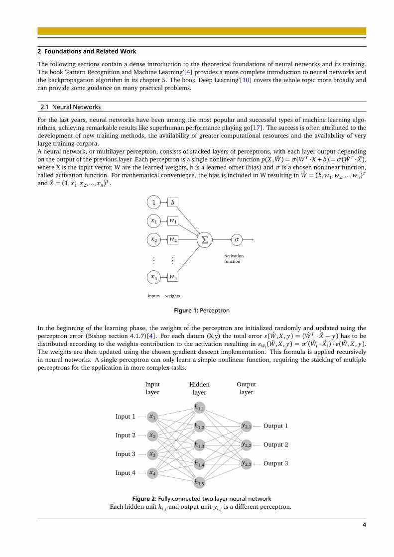
For the last years, neural networks have been among the most popular and successful types of machine learning algo-rithms, achieving remarkable results like superhuman performance playing go[17]. The success is often attributed to thedevelopment of new training methods, the availability of greater computational resources and the availability of verylarge training corpora.A neural network, or multilayer perceptron, consists of stacked layers of perceptrons, with each layer output dependingon the output of the previous layer. Each perceptron is a single nonlinear function p(X , W ) = σ(W T ·X + b) = σ(W T · X ),where X is the input vector, W are the learned weights, b is a learned offset (bias) and σ is a chosen nonlinear function,called activation function. For mathematical convenience, the bias is included in W resulting in W = (b, w1, w2, ..., wn)T

and X = (1, x1, x2, ..., xn)T .

Activationfunction

σ∑

w2x2

......

wnxn

w1x1

b1

inputs weights

Figure 1: Perceptron

In the beginning of the learning phase, the weights of the perceptron are initialized randomly and updated using theperceptron error (Bishop section 4.1.7)[4]. For each datum (X,y) the total error ε(W , X , y) = (W T · X − y) has to bedistributed according to the weights contribution to the activation resulting in εWi

(W , X , y) = σ′(Wi · X i) · ε(W , X , y).The weights are then updated using the chosen gradient descent implementation. This formula is applied recursivelyin neural networks. A single perceptron can only learn a simple nonlinear function, requiring the stacking of multipleperceptrons for the application in more complex tasks.

x1Input 1

x2Input 2

x3Input 3

x4Input 4

h1,1

h1,2

h1,3

h1,4

h1,5

y2,1 Output 1

y2,2 Output 2

y2,3 Output 3

Hiddenlayer

Inputlayer

Outputlayer

Figure 2: Fully connected two layer neural networkEach hidden unit hi, j and output unit yi, j is a different perceptron.

4

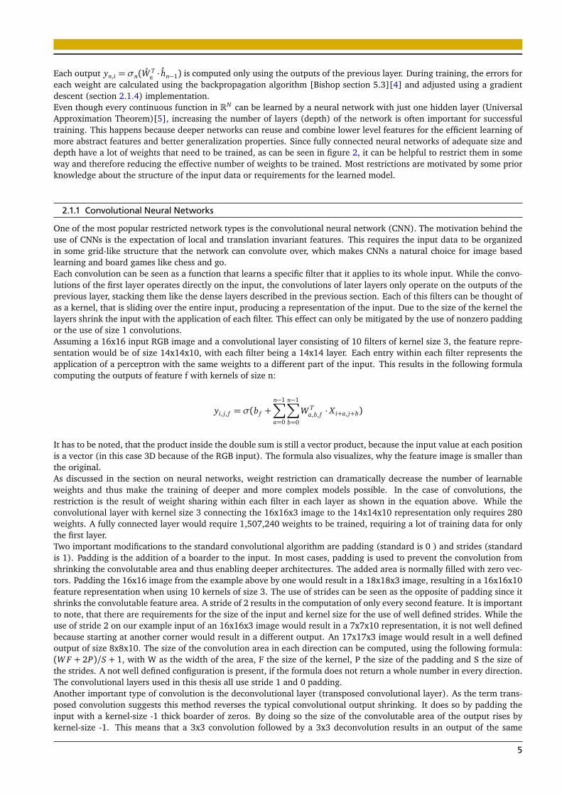
Each output yn,i = σn(W Tn · hn−1) is computed only using the outputs of the previous layer. During training, the errors for

each weight are calculated using the backpropagation algorithm [Bishop section 5.3][4] and adjusted using a gradientdescent (section 2.1.4) implementation.Even though every continuous function in RN can be learned by a neural network with just one hidden layer (UniversalApproximation Theorem)[5], increasing the number of layers (depth) of the network is often important for successfultraining. This happens because deeper networks can reuse and combine lower level features for the efficient learning ofmore abstract features and better generalization properties. Since fully connected neural networks of adequate size anddepth have a lot of weights that need to be trained, as can be seen in figure 2, it can be helpful to restrict them in someway and therefore reducing the effective number of weights to be trained. Most restrictions are motivated by some priorknowledge about the structure of the input data or requirements for the learned model.

2.1.1 Convolutional Neural Networks

One of the most popular restricted network types is the convolutional neural network (CNN). The motivation behind theuse of CNNs is the expectation of local and translation invariant features. This requires the input data to be organizedin some grid-like structure that the network can convolute over, which makes CNNs a natural choice for image basedlearning and board games like chess and go.Each convolution can be seen as a function that learns a specific filter that it applies to its whole input. While the convo-lutions of the first layer operates directly on the input, the convolutions of later layers only operate on the outputs of theprevious layer, stacking them like the dense layers described in the previous section. Each of this filters can be thought ofas a kernel, that is sliding over the entire input, producing a representation of the input. Due to the size of the kernel thelayers shrink the input with the application of each filter. This effect can only be mitigated by the use of nonzero paddingor the use of size 1 convolutions.Assuming a 16x16 input RGB image and a convolutional layer consisting of 10 filters of kernel size 3, the feature repre-sentation would be of size 14x14x10, with each filter being a 14x14 layer. Each entry within each filter represents theapplication of a perceptron with the same weights to a different part of the input. This results in the following formulacomputing the outputs of feature f with kernels of size n:

yi, j, f = σ(b f +n−1∑

a=0

n−1∑

b=0

W Ta,b, f · X i+a, j+b)

It has to be noted, that the product inside the double sum is still a vector product, because the input value at each positionis a vector (in this case 3D because of the RGB input). The formula also visualizes, why the feature image is smaller thanthe original.As discussed in the section on neural networks, weight restriction can dramatically decrease the number of learnableweights and thus make the training of deeper and more complex models possible. In the case of convolutions, therestriction is the result of weight sharing within each filter in each layer as shown in the equation above. While theconvolutional layer with kernel size 3 connecting the 16x16x3 image to the 14x14x10 representation only requires 280weights. A fully connected layer would require 1,507,240 weights to be trained, requiring a lot of training data for onlythe first layer.Two important modifications to the standard convolutional algorithm are padding (standard is 0 ) and strides (standardis 1). Padding is the addition of a boarder to the input. In most cases, padding is used to prevent the convolution fromshrinking the convolutable area and thus enabling deeper architectures. The added area is normally filled with zero vec-tors. Padding the 16x16 image from the example above by one would result in a 18x18x3 image, resulting in a 16x16x10feature representation when using 10 kernels of size 3. The use of strides can be seen as the opposite of padding since itshrinks the convolutable feature area. A stride of 2 results in the computation of only every second feature. It is importantto note, that there are requirements for the size of the input and kernel size for the use of well defined strides. While theuse of stride 2 on our example input of an 16x16x3 image would result in a 7x7x10 representation, it is not well definedbecause starting at another corner would result in a different output. An 17x17x3 image would result in a well definedoutput of size 8x8x10. The size of the convolution area in each direction can be computed, using the following formula:(W F + 2P)/S + 1, with W as the width of the area, F the size of the kernel, P the size of the padding and S the size ofthe strides. A not well defined configuration is present, if the formula does not return a whole number in every direction.The convolutional layers used in this thesis all use stride 1 and 0 padding.Another important type of convolution is the deconvolutional layer (transposed convolutional layer). As the term trans-posed convolution suggests this method reverses the typical convolutional output shrinking. It does so by padding theinput with a kernel-size -1 thick boarder of zeros. By doing so the size of the convolutable area of the output rises bykernel-size -1. This means that a 3x3 convolution followed by a 3x3 deconvolution results in an output of the same

5

convolutional area. The convolutional autoencoders used in this thesis and explained in the next section make use of thisproperty.

2.1.2 Autoencoder

An autoencoder takes an input datum, transforms it into an encoded representation and then decodes it back to some-thing close to the original. The encoding part of the network is referred to as the encoder, while the decoding part iscalled a decoder. All autoencoders constructed in this thesis are symmetric, resulting in encoder decoder pairs, with thesame hidden dimension in each layers. Because the decoder needs the reverse the encoding process its layers oder isreversed. Assuming an input of size 100 and encoding layers of the resulting sizes 80, 60 and 20 the resulting decoderwould use input of size 20 and produce layer outputs of size 60, 80 and 100.Since most tasks require labeled data, that is often very limited and expensive to acquire, unsupervised pre-training isoften successfully used for network initialization. Pre-training initializations are expected to be closer to solutions withbetter generalization properties [7]. Since the finding of representations that aid future learning is one of the major goalsof representation learning, autoencoders are a prominent tool in this domain.Because the objective function of an autoencoder only aims to reduce reconstruction errors the identity function wouldbe an optimal solution. In practice this does not happen if nonlinear layers are used in combination with early stoppingand stochastic gradient descent[2] and the use of convolutional layers without padding makes learning of the identityfunction even more infeasible.One very prominent way of forcing the network to generalize, is the training of a denoising autoencoder. In this archi-tecture, the input is changed by adding some random noise to it while the output remains unchanged. This leads to areward for generalization and in many cases to better overall performance, even though the noise level and distributionare new hyperparameters that need to be tuned. There is also the possibility of punishing encodings that are too complexthrough the introduction of regularization terms in the loss function. The most prominent regularizer is the L2 regularizerL(X ) = ||X ||2 which can be applied to the weights, or the activations of a layer, penalizing large weights or activations.This results in sparse neural activations which can improve performance.The usefulness of an autoencoder that is not used for pre-training can often only be evaluated through the application ofits encoding as preprocessing for a variety of tasks, making the evaluation a challenging task. The causes and possiblesolutions to this problem are further discussed in the evaluation section 3.2. It has to be noted that the application of anautoencoder relies on the assumption, that the training loss can guide to a useful representation of the data. In most usecases like pre-training this is not a real issue, because the same loss function is used in pre- and final-training, makingits usefulness apparent in the result in application task. This thesis tries to use the inherent board structure in a game ofchess as the basis of its feature extraction, which differs from previous chess based learning methods and is described insection 2.3.

2.1.3 Hyperparameter

Even though neural networks can learn their own representations of the given data they are not a black box solution andrequire a lot of parameters to be tuned. The choice of these parameters can themselves be interpreted as an learningproblem over all hyperparameters minimizing the loss of the network. Work on this front has been done by Andrychowiczet al.[1]. For large search-spaces and larger problems this method is very computationally demanding, because everyevaluation of the loss functions requires the complete training and evaluation of a network architecture, making it infea-sible in most situations.One of the most important and most complex hyperparameter types in a neural network is the layout of the architecture.Here the number of hidden layers, the number of neurons in each of these layer and connection restrictions betweenlayers have to be decided on. Many of these design decisions can be motivated by prior knowledge about the problemand the structure of the data. These parameters are often very hard to choose and are either engineered by trial anderror, heuristics or derived from previous architectures that address similar problems.The choice of the nonlinearities used for each layer is another important hyperparameter. Usually all neurons in onehidden layer use the same nonlinear function. In most modern architectures rectified linear units (ReLU) are used in allhidden layers. The output of a ReLU is 0 if the input is negative and its input if it is positive. This makes the computationof the function and its derivative very easy enabling the efficient training of deep networks. Another main advantageit that ReLUs seem to solve the vanishing gradient problem[9], which can occur during backpropagation in very deepnetworks when many small numbers need to be multiplied, because the ReLU output can be greater than 1. A differentimportant nonlinearity is the logistic function f (x) = 1

1+e−x , often referred to as sigmoid function, which forces the outputin [0, 1]. Its main use is in the output-layer of the network, where it can model degrees of confidence. This can be usefulfor tasks like multi-label classification. If all outputs should sum up to one, which would be a reasonable expectation intasks like multi-class classification, it is better to use the softmax function f (x)i =

exi∑K

j=1 ex j instead.

6

2.1.4 Gradient-Descent

Using the backpropagation algorithm on the loss produced by one training examples results in one error per weight. Thechoice of how this error should effect the weight update is taken by the gradient-descent implementation that is used fornetwork optimization.Given an error E(wi(tn)) the most crude implementation of a gradient-descent update would just perform the followingupdate: wi(tn+1) = wi(tn) − E(wi(tn)). Since the optimization problem of a multilayer perceptron is not convex, thisupdate is not guaranteed to reach the global optimum or even the best local optimum.There are three common additions to the normal gradient-descent algorithm that are often used to guide to bettersolutions. The introduction of a learning rate γ is the most common resulting in the following update function wi(tn+1) =wi(tn)−γE(wi(tn)). This can increase or decrease the size of the gradient steps and can improve convergence dramaticallyif chosen correctly. Fixed learning rates have the problem of being problem dependent, requiring fine-tuning and slowconvergence if the learning rate is chosen small enough for good convergence properties in later training stages. Thisproblem leads to a popular adaptation, a learning rate that is reduced over time. Most of the time this is achieved byusing a fixed decay resulting in the following learning rate update γ(tn+1) = c · γ(tn).Another popular modification is the introduction of momentum. Its main purpose is the avoidance of shallow localminima and the stabilization of the descent. This effect is achieved by adding an additional term resulting in the followingupdate wi(tn+1) = wi(tn)+Vi(tn+1)with Vi(tn+1) = µVi(tn)−γE(wi(tn)). Vi(tn+1) can be visualized as the current speed ofthe descent which depends on linear approximated friction µ, the previous speed Vi(tn) and the current slope γE(wi(tn)).Sufficient speed can enable the descent to get out of shallow local minima but - depending on the friction convergence- can be slower. Another advantage of momentum is its stabilizing property, preventing the descent form dramaticallychanging its direction in every step.When dealing with large amounts of data, which is the case in most deep learning applications, calculating the errorbased on the whole training set for a single gradient step becomes infeasible. A natural response to this problem isstochastic sampling. Here the used subset of the training data is sampled using a uniform distribution over the wholedata. Since this can not guarantee that every datum has the same impact on the weight it is advanced to its more popularsuccessors. In mini-batch gradient descent the data is randomly shuffled at the beginning of each epoch. The shuffleddata is then split in a fixed number of mini-batches on which the cumulative error is computed and backpropagated,resulting in multiple weight updated per epoch. This results in the positive properties of stochastic gradient descentcombined with more equal influence of the whole data. It is important to note that this does not ensure a high qualitygradient in every update or even the reaching of the same optimum when running multiple descents from the samestarting point, because unlucky sampling can still produce unrepresentative samples that guide the descent in the wrongway.The components discussed above are the main building blocks of most commonly used neural network optimizers. Theyoften use well tunes starting values and heuristics to ensure very good general convergence properties on real worldoptimization problems. In this thesis, the standard Keras implementation of Nadam, the addition of Nesterov Momentuminto Adam[13], is used together with mini-batch sampling to perform all the weight updated.

2.2 Representation Learning

The goal of representation learning is the discovery of features for a given data set that make a machine learning taskeasier. In the ideal case representation learning makes manual feature engineering obsolete. Traditional feature engi-neering required a lot of time and energy by experts. With the rise of deep learning and its inherent capability to learnand optimize its own features, machine learning areas like computer vision and natural language processing started toadvance much more rapidly, which enabled big performance boosts in tasks like speech recognition and autonomousdriving. While the advances in these areas are enormous, the requirement in computational power and training data forvery powerful models is too. This is one of the problems representation learning aims to solve.One prominent and very actively researched example is the finding of certain objects and their relative positions in animage, called object detection. While it is theoretically possible to train an end-to-end model receiving a video streamand converting it to actions steering a car, it is much more efficient to do this on the basis of the previous representation.In learning - as in many other domains - this modular approach has the added advantage of making testing feasibleby allowing the separate testing of every sub-model and thus ensuring that the right thing is learned. It also allowsfor reusability which can dramatically reduce training time and data requirements, making previously infeasible taskspossible.The creation of good general purpose representations is challenging if not impossible. Since every problem focuses ondifferent aspects of the data the learned representation is either to broad, requiring additional filtering, or not broadenough, omitting aspects relevant to some applications. In many cases is also not clear what features a good representa-tion should satisfy making the creation of a metric for learning challenging.Since the representation learned in this thesis has no specific application in mind, the main metric for training and eval-uation will be the reconstruction error. A low reconstruction error ensures, that most information present in the input is

7

still present in the output, which is one of the important properties of a general purpose representation discussed above.Therefore models building on the generated representation will likely have to learn which parts of the representation areimportant for them. The metrics used will be described at the end of the following section.

2.2.1 Unsupervised Representation Learning

Some representation learning tasks - such as labeling subsections of an image - require training data that has been la-beled by humans. This data is hard and expensive to come by or in domains like medical diagnostics sometimes noteven attainable. Unsupervised representation learning aims to get rid of this problem by not relying on any labeled data,which restricts the form of the resulting representation. This can be achieved by making the input equal the output (e.g.autoencoder) or by making input or output generatable (e.g. Jigsaw puzzles from images). Other unsupervised learningapproaches like clustering have no need for the generation of artificial input or output data.Since there is no target data that can guide the learning process, unsupervised learning is even more depending on hyper-parameter tuning than normal machine learning. In general these parameters are chosen according to the performanceon some tasks that are expected to represent its use cases.In this thesis an autoencoder is used as unsupervised representation learner. As described in section 2.1.2 it tries tofind a representation, that allows for a reconstruction with minimal errors. Further criteria by which the performance isevaluated are presented in section 3.2.2.

2.3 Related Work

2.3.1 CNN Visualization

The visualization of convolutional networks in the domain of image processing is a well researched area. Many of theapproaches presented in section 3.2.2 are adaptations of these methods. A good summarization of them was producedby Zeiler et al.[21]. Most of these techniques cannot be applied directly in the chess domain because of key differencesin the input. These differences and their consequences for visualization purposes are described in section 3.2.2.

2.3.2 Chess

Chess, and game playing in general, has always been a popular research topic in machine learning. While the bestchess programs can beat every human player, most rely on handcrafted and then optimized heuristics for final boardevaluation. This makes it an interesting research domain for the development of different strategies. In 2015 a programcalled Giraffe[15] was able to reach FIDE-IM level playing strength ( 2,400 elo) using reinforcement learning. DeepChess[6] was also developed in 2015 and was able to play at FIDE-GM level ( 2,500 elo) using several million expert gamesfor training. Both approaches relied on dense neural network architectures.

8

3 Methodology

3.1 Training

The autoencoder was trained as a symmetric convolutional model, resulting in a decoder that produces intermediate out-puts of the same dimension as the encoder. This can be achieved using the transpose convolution operation. The modelssuccess was evaluated using MSE on unseen validation examples and was optimize using the following parameters:

1. number and shape of the convolutional layers

2. activation functions

3. dropout rate

4. input noise

This resulted in an autoencoder that was able to reconstruct 99% of the validation examples flawlessly after discretization.The exact results are presented in section 4.2.

3.1.1 Autoencoder Layout and Nomenclature

This section describes the general layout of all used autoencoders and the nomenclature by which they will be referredto in this thesis.All autoencoders use convolutions in most of their layers with 0 padding and strides 1, which ensures, that the input isgetting compressed. The remaining differences between the layers are kernel size, layer depth, and nonlinearity, whichwill be specified in the following way:

3x3-60|2x2-90|2x2-120|2x2-225|250|relu_sigmoid

Figure 3: Example autoencoder nomenclature

The first part describes the layout of the layers, seperating each one by ’|’. The example encoder consists of four con-volutional layers and one dense layer. The first encoding layer uses a 3x3x60 kernel transforming the 8x8x12 shapedinput into a 6x6x60 encoding, on which the second layer operates. The last layer is a dense layer, which is shown by themissing kernel size. It uses the 3x3x225 encoding resulting from the 2x2x225 kernel and transforms it in 250 output bits.The decoder does the same operations in reverse, transforming its 250 bit input into a 2025 bit output, getting reshapedinto 3x3x225 bit and reversing the encoding process using a 2x2x120 deconvolutional layer.The next two parameters specify the used nonlinear functions, where the first specifies the type of activation in all butthe final encoder and decoder layers and the second the type of activation in final encoder layer. In this example ReLUsare used for all layers beside the final encoding and decoding layer. The last decoding layer always uses a sigmoid non-linearity, because it tries to predict binary values. In the example above a sigmoid function is used as nonlinearity usedfor the last encoding layer.If dropout is used it is used in front of every layer while training and the dropout rate is specified separately. Input noiseand its noise rate are specified separately if used.

3.2 Autoencoder Evaluation

The performance assessment of an autoencoder is different from most machine learning tasks. This is due to the fact,that meaningful performance measures are much harder to find, because the quality of the produced encoding is hardto measure. Useful training and evaluation become much more difficult, because the successful reconstruction is only abyproduct is not the goal of autoencoders, even though it is the metric used by their optimization process. As discussedin section 2.2 the goal of an autoencoder is the finding of an useful representation of the given data. Because the generalusefulness of a representation cannot be be measured it is tried to be approximated using three types of evaluation. Forthis reason the generated models were compared in their reconstruction error, visualization and application.The quality of the reconstruction is the one of the central metrics when evaluating. If the central assumption behind theuse of autoencoders, that a useful representation can be found through encoding and decoding, is correct the reconstruc-tion error is a good measure for the evaluation of the architecture. This assumption does not have to be correct, becausewhile it is true, that the autoencoder needs to exploit some structures of the training data to learn a good encoding anddecoding procedure the found encodings do not have to be useful for any other applications.One of the many appeals of CNN’s, especially the ones using 2 dimensional convolutions, is the ability to visualize its

9

activations as a 2D image, wich is one of the key ingredients of the visualizations presented in section 3.2.2. This can bea very helpful tool during development and is popular in image processing tasks.Since the goal of the encoding is the learning of structures, which are present in high quality chess positions, there aresome natural application on which the quality can be assessed. These applications are the last part of the followingsubsections.

3.2.1 Reconstruction

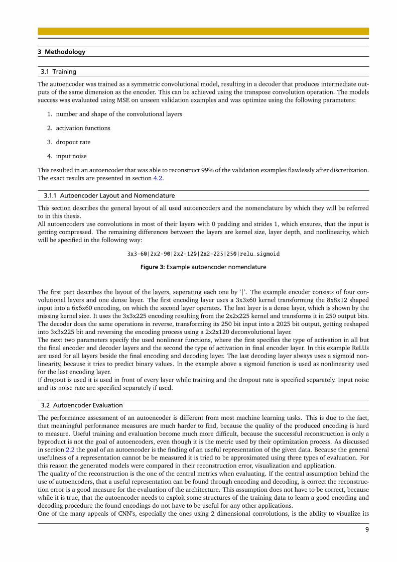
The most straight forward and the only metric on which the autoencoder can actually be trained is the quality of thereconstruction. If the data is represented in a way, that allows a very accurate reconstruction of the original data it isensured, that only few information is lost through the encoding process. Depending on the application using the encodeddata this can be more or less desirable, because may tasks require only a portion of the provided information. Sincethe desirable information depends on the task it is reasonable to assume, that this is a necessary, but not sufficient,property of a general purpose representation. This property will be measured using the mean squared error (MSE) of thereconstructed boards. During training the continuous outputs of the final layers are used to provide better gradients. Forevaluation the output is discretized allowing for a better quality assessment.During training The quality of the output was evaluated using the following criteria:

• error rates per board (discrete)

• MSE (discrete)/board

• MSE /board

• MSE /bit (loss)

For the discrete evaluation methods the error was computed using the rounded predicted output (rounding 0.5 to 0),resulting in the following sample prediction.

number of errors MSE(dis) MSE loss0 1 2 3 4 5 6 7 8 9 >=10

0.63 0.26 0.08 0.02 0.00 0.00 0.00 0.00 0.00 0.00 0.00 0.87 0.54 0.0007

Figure 4: Evaluation exampleEvaluation of an autoencoder which recreated 63% of the unseen positions correctly.

This evaluation gives a much better sense of the actual performance of the generated model. All errors are computedusing the bitwise difference between the prediction and the actual output, resulting in an error of two when a pieceshould be moved to another empty position.

3.2.2 Visualization

While the performance on a specific task is an important part of the evaluation process an understanding of what hasbeen learned is helpful for ensuring good generalization properties. This is important, because nearly all datasets aresubject to some inherent sampling biases. A famous example for the problems that can arise when training a neuralnetwork without visualization can be found in a story, in which a network was supposedly able to perfectly separatepictures of enemy tanks from pictures without them, while in reality it was only able to separate cloudy from sunnypictures[20]. While these errors are easy to recognize after the fact it is very difficult to create training examples thatcannot be reward-hacked (the substitution of the original task by an unintended, simpler to achieve task that does notsolve the intended problem, but satisfies its reward function) by the network. This has always been an advantage ofeasier to interpret methods like rule learning over methods like neural networks.Convolutional networks have, thanks to their inherent structure, an advantage over the other network architectures. Thisis the case because they convolute over time (1-D) or space (2-D) which results in network layers that preserve this shapeand thus are easier to visualize. Many visualization techniques rely on the inherent properties of images, making their usefor higher dimensional and discrete domains like chess boards challenging. Another problem is the information densityof a chess position. When looking at natural images the color values of a given pixel often correlate with the values ofadjacent pixels, while the state of one chess tile does often not contain a lot of information about the state of adjacenttiles. These problems together with the small overall size of the original input (8x8) over which is being convoluted,make the visualization and learning of meaningful features very challenging.

10

Since chess positions differ from pictures in many ways, the methods developed in computer vision are not easily trans-ferable. Even though each position can be efficiently represented using an 2-D array, because each field can only containone piece at each time, some visualization techniques rely on continuous values for each piece-type. This requirement isdifficult, because a tile with half a pawn on it cannot be easily visualized. While colored images have three dimensionsper pixel which can be shown simultaneously, chess positions have 12 (every color, chess-piece pair) , or at least 7 (coloras seventh dimension) dimensions per chess-tile which restricts visualization possibilities dramatically. The followingsections contain information to the visualization techniques that have been applied.

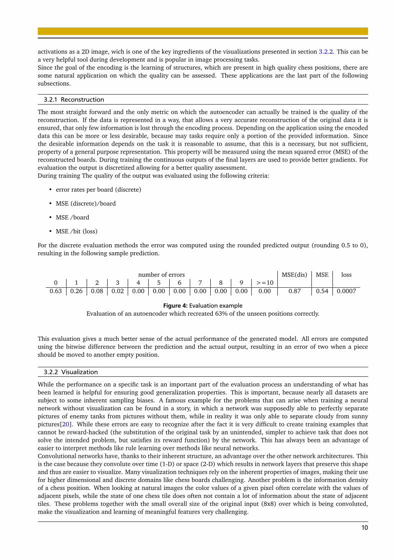
Weight VisualizationThe visualization of the weights of the first layer is one of the most common techniques for many convolutional networks.The weights of deeper layers can not be easily interpreted using this technique, because their weights only combine thenonlinear output of the previous layers and not the input layer. This technique has been used to visualize the first layerof AlexNet[14] the winner of the 2012 ImageNet Large Scale Visual Recognition Challenge[16]. Its visualization showsa variety of edges, patterns and color transitions. These kinds of transitions can also be observed in many other convo-lutional image based networks with sufficiently large first layer kernels. While earlier networks like AlexNet can allowfor larger convolutional kernels in their first layers, 11x11 in the case of AlexNet, more recent networks like Inception-ResNet[19] are much deeper and thus can’t afford the use of large input kernels (3x3 in its first layers). This results inthe loss of interpretability, because edges are often larger than the first kernels.Since the primitives found in the first image layers are also the most fundamental features previously designed by expertsit is interesting to find out, whether the patterns chosen by this autoencoder have similarly recognizable forms.

Figure 5: Weight visualization exampleExample weight visualization with synthetic generated weight. The Weights are initialized randomly and a diagonal

weight of 1 is added for white and black pawns. Pieces types are from left to right Pawn, Knight, Bishop, Rook, Queen,King with alternating colors, starting with white.

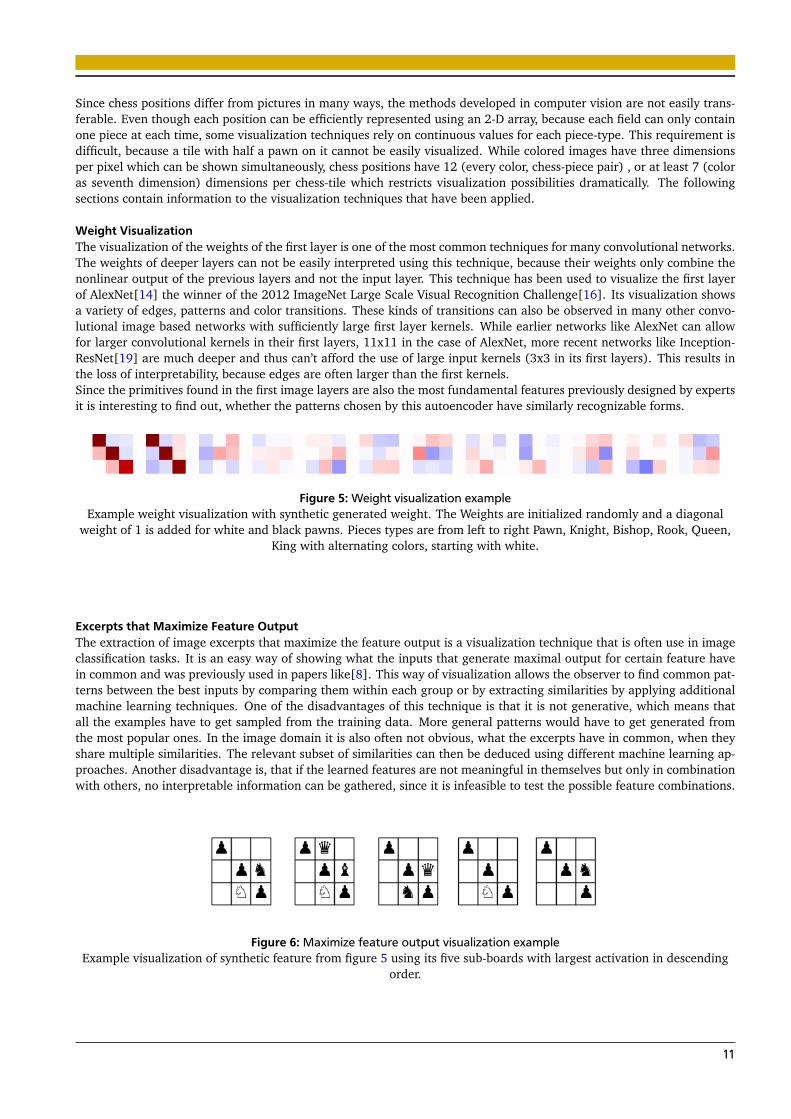
Excerpts that Maximize Feature OutputThe extraction of image excerpts that maximize the feature output is a visualization technique that is often use in imageclassification tasks. It is an easy way of showing what the inputs that generate maximal output for certain feature havein common and was previously used in papers like[8]. This way of visualization allows the observer to find common pat-terns between the best inputs by comparing them within each group or by extracting similarities by applying additionalmachine learning techniques. One of the disadvantages of this technique is that it is not generative, which means thatall the examples have to get sampled from the training data. More general patterns would have to get generated fromthe most popular ones. In the image domain it is also often not obvious, what the excerpts have in common, when theyshare multiple similarities. The relevant subset of similarities can then be deduced using different machine learning ap-proaches. Another disadvantage is, that if the learned features are not meaningful in themselves but only in combinationwith others, no interpretable information can be gathered, since it is infeasible to test the possible feature combinations.

Figure 6: Maximize feature output visualization exampleExample visualization of synthetic feature from figure 5 using its five sub-boards with largest activation in descending

order.

11

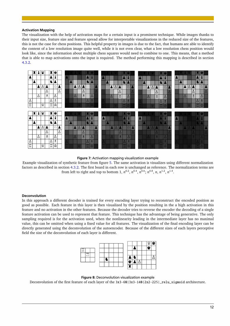
Activation MappingThe visualization with the help of activation maps for a certain input is a prominent technique. While images thanks totheir input size, feature size and feature spread allow for interpretable visualizations in the reduced size of the features,this is not the case for chess positions. This helpful property in images is due to the fact, that humans are able to identifythe content of a low resolution image quite well, while it is not even clear, what a low resolution chess position wouldlook like, since the information about multiple chess squares would need to combine to one. This means, that a methodthat is able to map activations onto the input is required. The method performing this mapping is described in section4.3.2.

Figure 7: Activation mapping visualization exampleExample visualization of synthetic feature from figure 5. The same activation is visualizes using different normalizationfactors as described in section 4.3.2. The first board in each row is unchanged as reference. The normalization terms are

from left to right and top to bottom 1, n0.2, n0.4, n0.6; n0.8, n, n1.2, n1.4.

DeconvolutionIn this approach a different decoder is trained for every encoding layer trying to reconstruct the encoded position asgood as possible. Each feature in this layer is then visualized by the position resulting in the a high activation in thisfeature and no activation in the other features. Because the decoder tries to reverse the encoder the decoding of a singlefeature activation can be used to represent that feature. This technique has the advantage of being generative. The onlysampling required is for the activation used, when the nonlinearity leading in the intermediate layer has no maximalvalue, this can be omitted when using a fixed value for all features. The visualization of the final encoding layer can bedirectly generated using the deconvolution of the autoencoder. Because of the different sizes of each layers perceptivefield the size of the deconvolution of each layer is different.

Figure 8: Deconvolution visualization exampleDeconvolution of the first feature of each layer of the 3x3-60|3x3-140|2x2-225|_relu_sigmoid architecture.

12

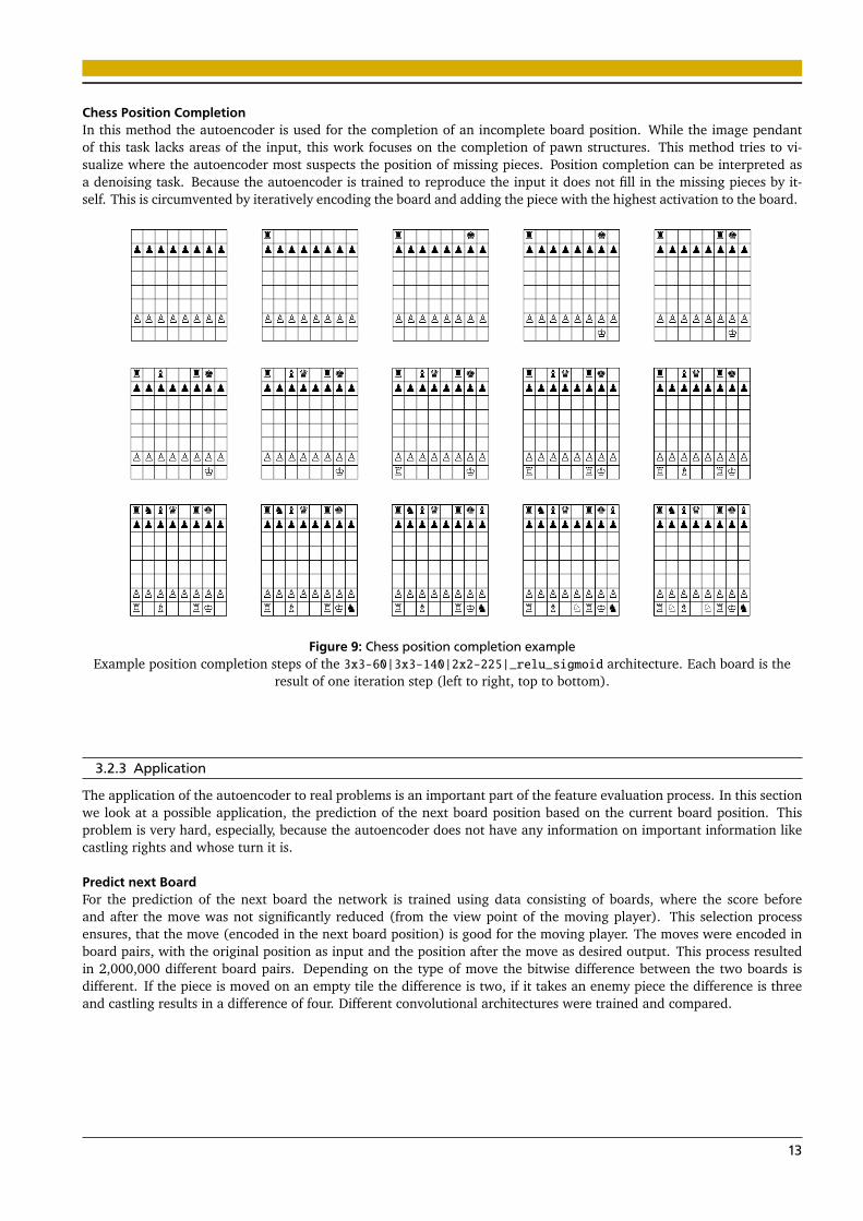
Chess Position CompletionIn this method the autoencoder is used for the completion of an incomplete board position. While the image pendantof this task lacks areas of the input, this work focuses on the completion of pawn structures. This method tries to vi-sualize where the autoencoder most suspects the position of missing pieces. Position completion can be interpreted asa denoising task. Because the autoencoder is trained to reproduce the input it does not fill in the missing pieces by it-self. This is circumvented by iteratively encoding the board and adding the piece with the highest activation to the board.

Figure 9: Chess position completion exampleExample position completion steps of the 3x3-60|3x3-140|2x2-225|_relu_sigmoid architecture. Each board is the

result of one iteration step (left to right, top to bottom).

3.2.3 Application

The application of the autoencoder to real problems is an important part of the feature evaluation process. In this sectionwe look at a possible application, the prediction of the next board position based on the current board position. Thisproblem is very hard, especially, because the autoencoder does not have any information on important information likecastling rights and whose turn it is.

Predict next BoardFor the prediction of the next board the network is trained using data consisting of boards, where the score beforeand after the move was not significantly reduced (from the view point of the moving player). This selection processensures, that the move (encoded in the next board position) is good for the moving player. The moves were encoded inboard pairs, with the original position as input and the position after the move as desired output. This process resultedin 2,000,000 different board pairs. Depending on the type of move the bitwise difference between the two boards isdifferent. If the piece is moved on an empty tile the difference is two, if it takes an enemy piece the difference is threeand castling results in a difference of four. Different convolutional architectures were trained and compared.

13

4 Experiments and Evaluation

4.1 Data

The used data was generated using approximately 700,000 chess-games in PGN notation (see figure 10) from chess-db.com. All games with at least one player below 2,500 elo (the most common chess player skill ranking scheme) orblitz-games (games with reduced game duration) were removed. The resulting games were then converted into a set ofpositions and then filtered using the following criteria:

1. The evaluation of the position is between -100 and 100 centi-pawns (using Stockfish 7).

2. Both players have the same number of pieces of the same value.

One centi-pawn is defined as 1100 the value of a pawn. The sigh of the evaluation is negative if black has an advantage

and positive otherwise. Since chess is a zero-sum game the balance of a given position can be represented using only onenumber, because an advantage for white is always a disadvantage for black. Because Chess programs like Stockfish usea tree search algorithm they require a good metric for the evaluation of positions to decide which outcome is the mostfavorable. These metrics are very fine tuned heuristics including features like material, pawn structure and king safety.The balance of the used positions is important because the autoencoder is expected to only learn structures, that arepresent in well balanced chess positions. To prevent positions that are in the middle of an exchange the second filteringcriterion was used. It ensures an equal number of pieces with equal value (queen; rook; bishop, knight; pawn).This resulted in 3 million unique positions, of which 500 000 were hold back for the final evaluation and the remainingwere split into 90% training and 10% validation data. Due to the space requirements of the expanded bitmaps the posi-tions are saved using standard FEN notation and 8x8x12 bitmaps were created during training.In each bitmap the first 12 dimensions encode the presence (1) or absence (0) of one of the 12 chess piece, player colorcombinations, while the last 8x8 represent the positions on the chess board. This representation discards some informa-tions like castling rights and which players turn it is, which are vital for the prediction of the outcome of a chess game,for the sake of allowing the use of pure convolutional layers.

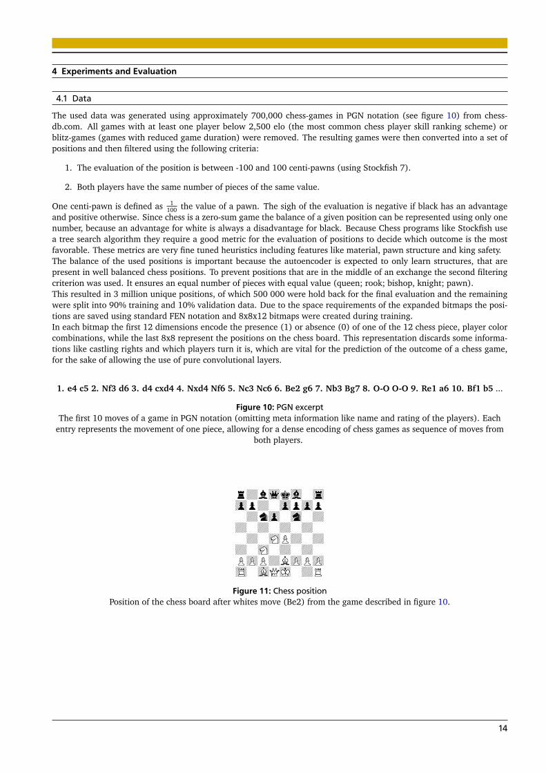
1. e4 c5 2. Nf3 d6 3. d4 cxd4 4. Nxd4 Nf6 5. Nc3 Nc6 6. Be2 g6 7. Nb3 Bg7 8. O-O O-O 9. Re1 a6 10. Bf1 b5 ...

Figure 10: PGN excerptThe first 10 moves of a game in PGN notation (omitting meta information like name and rating of the players). Each

entry represents the movement of one piece, allowing for a dense encoding of chess games as sequence of moves fromboth players.

Figure 11: Chess positionPosition of the chess board after whites move (Be2) from the game described in figure 10.

14

Internally the extracted positions are stored using their FEN representation (one of the most common ways of encodinga chess position).

r1bqkb1r/pp2pppp/2np1n2/8/3NP3/2N5/PPP1BPPP/R1BQK2R b KQkq - 4 6

Figure 12: FENFEN encoding of the position in figure 11.

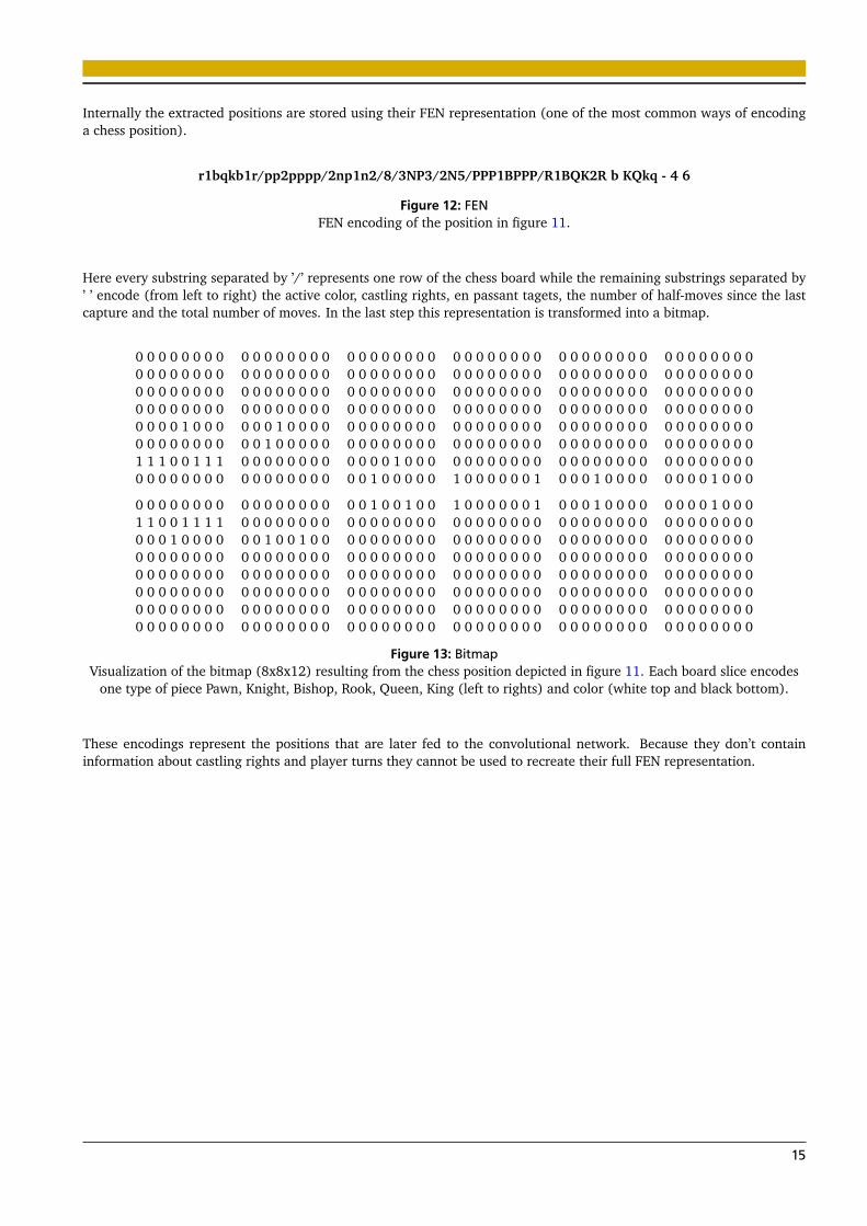
Here every substring separated by ’/’ represents one row of the chess board while the remaining substrings separated by’ ’ encode (from left to right) the active color, castling rights, en passant tagets, the number of half-moves since the lastcapture and the total number of moves. In the last step this representation is transformed into a bitmap.

0 0 0 0 0 0 0 0 0 0 0 0 0 0 0 0 0 0 0 0 0 0 0 0 0 0 0 0 0 0 0 0 0 0 0 0 0 0 0 0 0 0 0 0 0 0 0 00 0 0 0 0 0 0 0 0 0 0 0 0 0 0 0 0 0 0 0 0 0 0 0 0 0 0 0 0 0 0 0 0 0 0 0 0 0 0 0 0 0 0 0 0 0 0 00 0 0 0 0 0 0 0 0 0 0 0 0 0 0 0 0 0 0 0 0 0 0 0 0 0 0 0 0 0 0 0 0 0 0 0 0 0 0 0 0 0 0 0 0 0 0 00 0 0 0 0 0 0 0 0 0 0 0 0 0 0 0 0 0 0 0 0 0 0 0 0 0 0 0 0 0 0 0 0 0 0 0 0 0 0 0 0 0 0 0 0 0 0 00 0 0 0 1 0 0 0 0 0 0 1 0 0 0 0 0 0 0 0 0 0 0 0 0 0 0 0 0 0 0 0 0 0 0 0 0 0 0 0 0 0 0 0 0 0 0 00 0 0 0 0 0 0 0 0 0 1 0 0 0 0 0 0 0 0 0 0 0 0 0 0 0 0 0 0 0 0 0 0 0 0 0 0 0 0 0 0 0 0 0 0 0 0 01 1 1 0 0 1 1 1 0 0 0 0 0 0 0 0 0 0 0 0 1 0 0 0 0 0 0 0 0 0 0 0 0 0 0 0 0 0 0 0 0 0 0 0 0 0 0 00 0 0 0 0 0 0 0 0 0 0 0 0 0 0 0 0 0 1 0 0 0 0 0 1 0 0 0 0 0 0 1 0 0 0 1 0 0 0 0 0 0 0 0 1 0 0 0

0 0 0 0 0 0 0 0 0 0 0 0 0 0 0 0 0 0 1 0 0 1 0 0 1 0 0 0 0 0 0 1 0 0 0 1 0 0 0 0 0 0 0 0 1 0 0 01 1 0 0 1 1 1 1 0 0 0 0 0 0 0 0 0 0 0 0 0 0 0 0 0 0 0 0 0 0 0 0 0 0 0 0 0 0 0 0 0 0 0 0 0 0 0 00 0 0 1 0 0 0 0 0 0 1 0 0 1 0 0 0 0 0 0 0 0 0 0 0 0 0 0 0 0 0 0 0 0 0 0 0 0 0 0 0 0 0 0 0 0 0 00 0 0 0 0 0 0 0 0 0 0 0 0 0 0 0 0 0 0 0 0 0 0 0 0 0 0 0 0 0 0 0 0 0 0 0 0 0 0 0 0 0 0 0 0 0 0 00 0 0 0 0 0 0 0 0 0 0 0 0 0 0 0 0 0 0 0 0 0 0 0 0 0 0 0 0 0 0 0 0 0 0 0 0 0 0 0 0 0 0 0 0 0 0 00 0 0 0 0 0 0 0 0 0 0 0 0 0 0 0 0 0 0 0 0 0 0 0 0 0 0 0 0 0 0 0 0 0 0 0 0 0 0 0 0 0 0 0 0 0 0 00 0 0 0 0 0 0 0 0 0 0 0 0 0 0 0 0 0 0 0 0 0 0 0 0 0 0 0 0 0 0 0 0 0 0 0 0 0 0 0 0 0 0 0 0 0 0 00 0 0 0 0 0 0 0 0 0 0 0 0 0 0 0 0 0 0 0 0 0 0 0 0 0 0 0 0 0 0 0 0 0 0 0 0 0 0 0 0 0 0 0 0 0 0 0

Figure 13: BitmapVisualization of the bitmap (8x8x12) resulting from the chess position depicted in figure 11. Each board slice encodes

one type of piece Pawn, Knight, Bishop, Rook, Queen, King (left to rights) and color (white top and black bottom).

These encodings represent the positions that are later fed to the convolutional network. Because they don’t containinformation about castling rights and player turns they cannot be used to recreate their full FEN representation.

15

4.2 Autoencoder Training

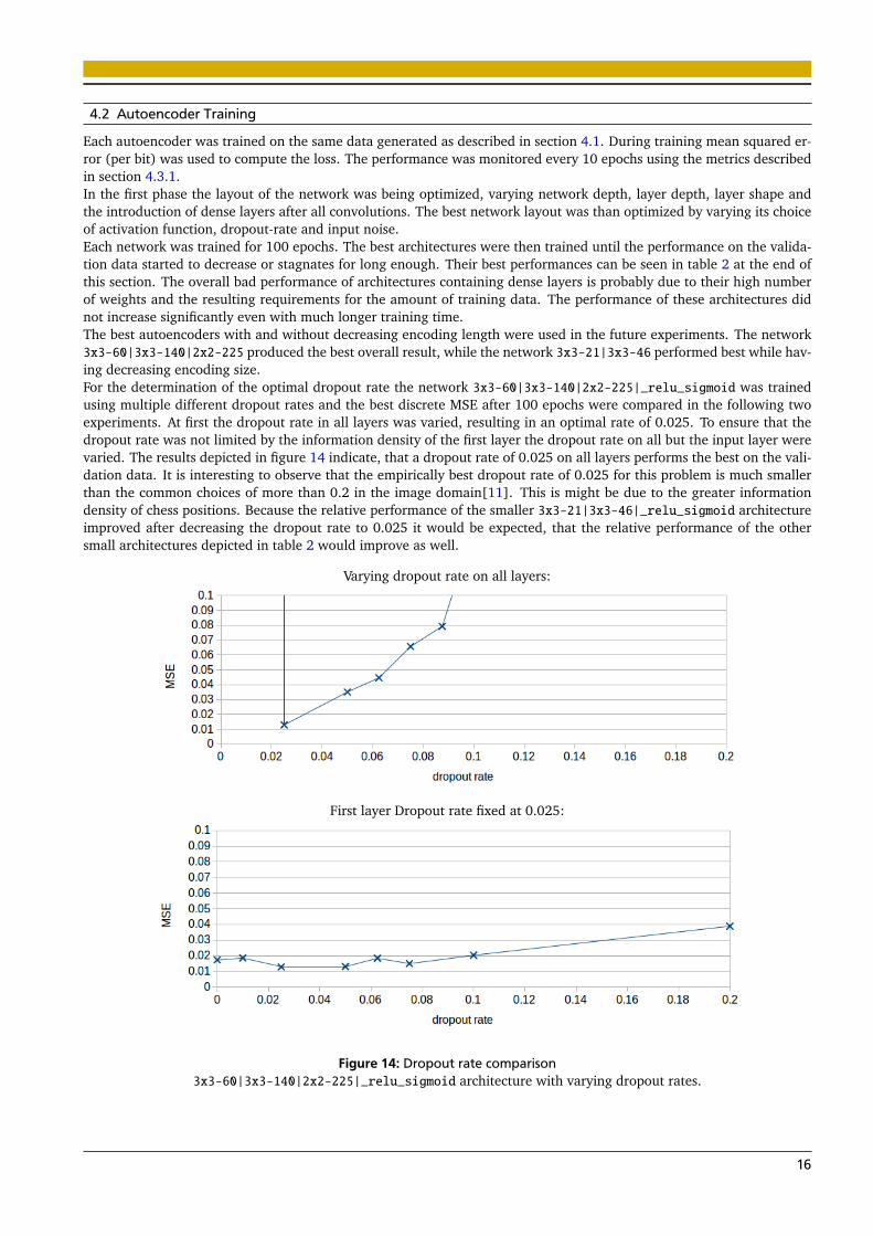
Each autoencoder was trained on the same data generated as described in section 4.1. During training mean squared er-ror (per bit) was used to compute the loss. The performance was monitored every 10 epochs using the metrics describedin section 4.3.1.In the first phase the layout of the network was being optimized, varying network depth, layer depth, layer shape andthe introduction of dense layers after all convolutions. The best network layout was than optimized by varying its choiceof activation function, dropout-rate and input noise.Each network was trained for 100 epochs. The best architectures were then trained until the performance on the valida-tion data started to decrease or stagnates for long enough. Their best performances can be seen in table 2 at the end ofthis section. The overall bad performance of architectures containing dense layers is probably due to their high numberof weights and the resulting requirements for the amount of training data. The performance of these architectures didnot increase significantly even with much longer training time.The best autoencoders with and without decreasing encoding length were used in the future experiments. The network3x3-60|3x3-140|2x2-225 produced the best overall result, while the network 3x3-21|3x3-46 performed best while hav-ing decreasing encoding size.For the determination of the optimal dropout rate the network 3x3-60|3x3-140|2x2-225|_relu_sigmoid was trainedusing multiple different dropout rates and the best discrete MSE after 100 epochs were compared in the following twoexperiments. At first the dropout rate in all layers was varied, resulting in an optimal rate of 0.025. To ensure that thedropout rate was not limited by the information density of the first layer the dropout rate on all but the input layer werevaried. The results depicted in figure 14 indicate, that a dropout rate of 0.025 on all layers performs the best on the vali-dation data. It is interesting to observe that the empirically best dropout rate of 0.025 for this problem is much smallerthan the common choices of more than 0.2 in the image domain[11]. This is might be due to the greater informationdensity of chess positions. Because the relative performance of the smaller 3x3-21|3x3-46|_relu_sigmoid architectureimproved after decreasing the dropout rate to 0.025 it would be expected, that the relative performance of the othersmall architectures depicted in table 2 would improve as well.

Varying dropout rate on all layers:

First layer Dropout rate fixed at 0.025:

Figure 14: Dropout rate comparison3x3-60|3x3-140|2x2-225|_relu_sigmoid architecture with varying dropout rates.

16

In the next experiment the 3x3-60|3x3-140|2x2-225 network was optimized in its choice of activation functions. Whilethe output activation function was fixed due to the constrains by the bitmap output, the different activations in the re-maining layers were not. The activations considered were Sigmoid and ReLU. They were varied in the final encodinglayer and in all remaining layers.

Table 1: Activation comparisonnumber of errors MSE(dis) architecture

0 1 2 3 ≥ 40.986 0.013 0.0 0.0 0.0 0.015 relu_sigmoid

0.985 0.015 0.001 0.0 0.0 0.018 sigmoid_sigmoid

0.982 0.017 0.001 0.0 0.0 0.023 sigmoid_relu

0.095 0.174 0.243 0.205 0.283 7.678 relu_relu

validation performance of different activation combinations with a dropout rate of 0.025 using the3x3-60|3x3-140|2x2-225 architecture.

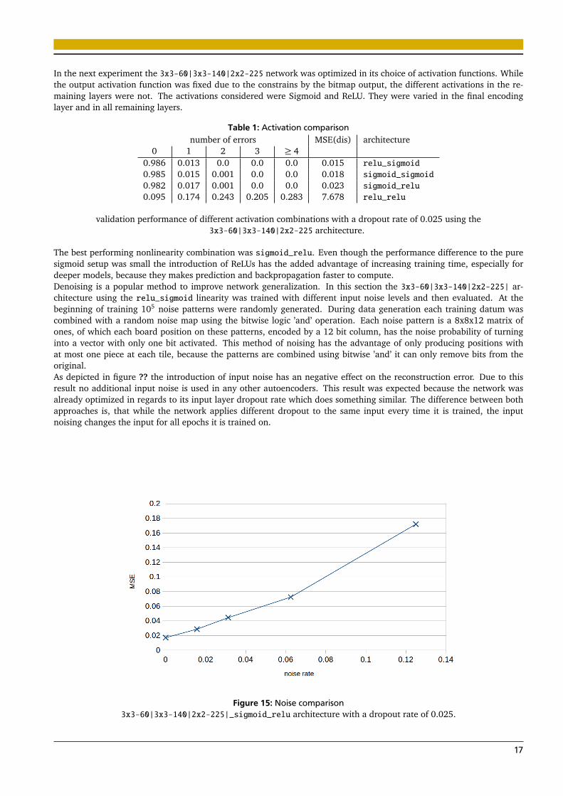
The best performing nonlinearity combination was sigmoid_relu. Even though the performance difference to the puresigmoid setup was small the introduction of ReLUs has the added advantage of increasing training time, especially fordeeper models, because they makes prediction and backpropagation faster to compute.Denoising is a popular method to improve network generalization. In this section the 3x3-60|3x3-140|2x2-225| ar-chitecture using the relu_sigmoid linearity was trained with different input noise levels and then evaluated. At thebeginning of training 105 noise patterns were randomly generated. During data generation each training datum wascombined with a random noise map using the bitwise logic ’and’ operation. Each noise pattern is a 8x8x12 matrix ofones, of which each board position on these patterns, encoded by a 12 bit column, has the noise probability of turninginto a vector with only one bit activated. This method of noising has the advantage of only producing positions withat most one piece at each tile, because the patterns are combined using bitwise ’and’ it can only remove bits from theoriginal.As depicted in figure ?? the introduction of input noise has an negative effect on the reconstruction error. Due to thisresult no additional input noise is used in any other autoencoders. This result was expected because the network wasalready optimized in regards to its input layer dropout rate which does something similar. The difference between bothapproaches is, that while the network applies different dropout to the same input every time it is trained, the inputnoising changes the input for all epochs it is trained on.

Figure 15: Noise comparison3x3-60|3x3-140|2x2-225|_sigmoid_relu architecture with a dropout rate of 0.025.

17

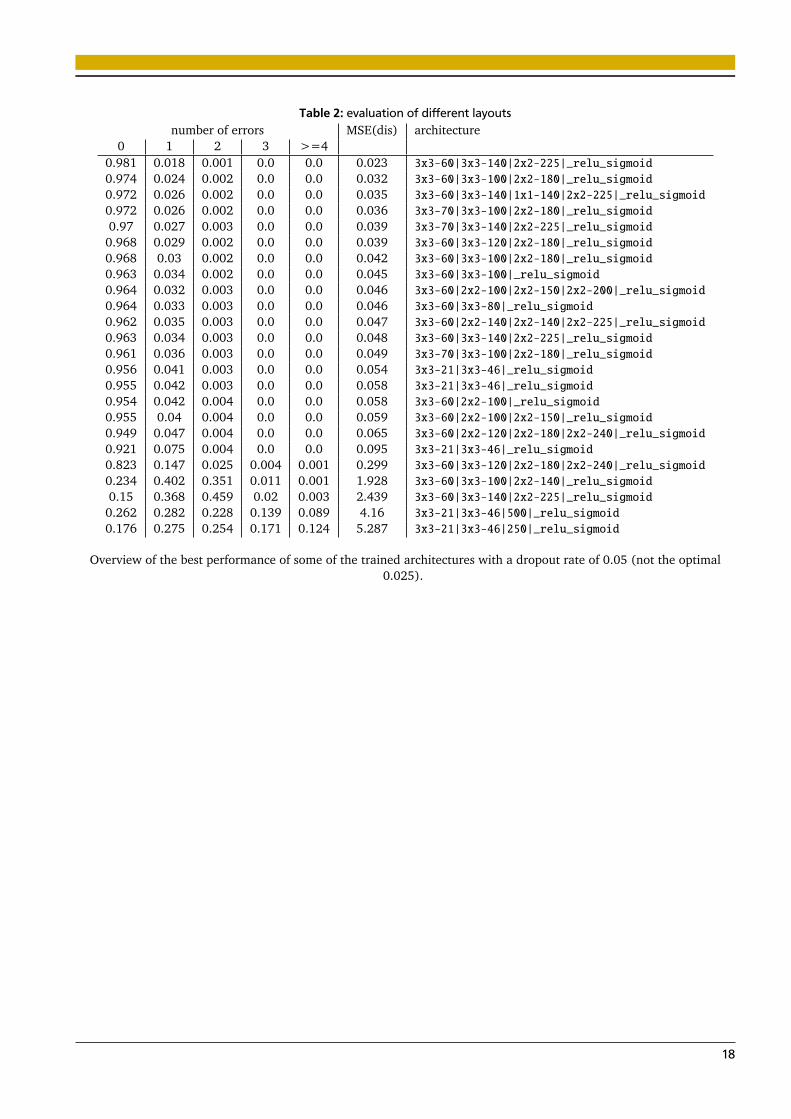
Table 2: evaluation of different layoutsnumber of errors MSE(dis) architecture

0 1 2 3 >=40.981 0.018 0.001 0.0 0.0 0.023 3x3-60|3x3-140|2x2-225|_relu_sigmoid

0.974 0.024 0.002 0.0 0.0 0.032 3x3-60|3x3-100|2x2-180|_relu_sigmoid

0.972 0.026 0.002 0.0 0.0 0.035 3x3-60|3x3-140|1x1-140|2x2-225|_relu_sigmoid

0.972 0.026 0.002 0.0 0.0 0.036 3x3-70|3x3-100|2x2-180|_relu_sigmoid

0.97 0.027 0.003 0.0 0.0 0.039 3x3-70|3x3-140|2x2-225|_relu_sigmoid

0.968 0.029 0.002 0.0 0.0 0.039 3x3-60|3x3-120|2x2-180|_relu_sigmoid

0.968 0.03 0.002 0.0 0.0 0.042 3x3-60|3x3-100|2x2-180|_relu_sigmoid

0.963 0.034 0.002 0.0 0.0 0.045 3x3-60|3x3-100|_relu_sigmoid

0.964 0.032 0.003 0.0 0.0 0.046 3x3-60|2x2-100|2x2-150|2x2-200|_relu_sigmoid

0.964 0.033 0.003 0.0 0.0 0.046 3x3-60|3x3-80|_relu_sigmoid

0.962 0.035 0.003 0.0 0.0 0.047 3x3-60|2x2-140|2x2-140|2x2-225|_relu_sigmoid

0.963 0.034 0.003 0.0 0.0 0.048 3x3-60|3x3-140|2x2-225|_relu_sigmoid

0.961 0.036 0.003 0.0 0.0 0.049 3x3-70|3x3-100|2x2-180|_relu_sigmoid

0.956 0.041 0.003 0.0 0.0 0.054 3x3-21|3x3-46|_relu_sigmoid

0.955 0.042 0.003 0.0 0.0 0.058 3x3-21|3x3-46|_relu_sigmoid

0.954 0.042 0.004 0.0 0.0 0.058 3x3-60|2x2-100|_relu_sigmoid

0.955 0.04 0.004 0.0 0.0 0.059 3x3-60|2x2-100|2x2-150|_relu_sigmoid

0.949 0.047 0.004 0.0 0.0 0.065 3x3-60|2x2-120|2x2-180|2x2-240|_relu_sigmoid

0.921 0.075 0.004 0.0 0.0 0.095 3x3-21|3x3-46|_relu_sigmoid

0.823 0.147 0.025 0.004 0.001 0.299 3x3-60|3x3-120|2x2-180|2x2-240|_relu_sigmoid

0.234 0.402 0.351 0.011 0.001 1.928 3x3-60|3x3-100|2x2-140|_relu_sigmoid

0.15 0.368 0.459 0.02 0.003 2.439 3x3-60|3x3-140|2x2-225|_relu_sigmoid

0.262 0.282 0.228 0.139 0.089 4.16 3x3-21|3x3-46|500|_relu_sigmoid

0.176 0.275 0.254 0.171 0.124 5.287 3x3-21|3x3-46|250|_relu_sigmoid

Overview of the best performance of some of the trained architectures with a dropout rate of 0.05 (not the optimal0.025).

18

4.3 Autoencoder Evaluation

4.3.1 Reconstruction

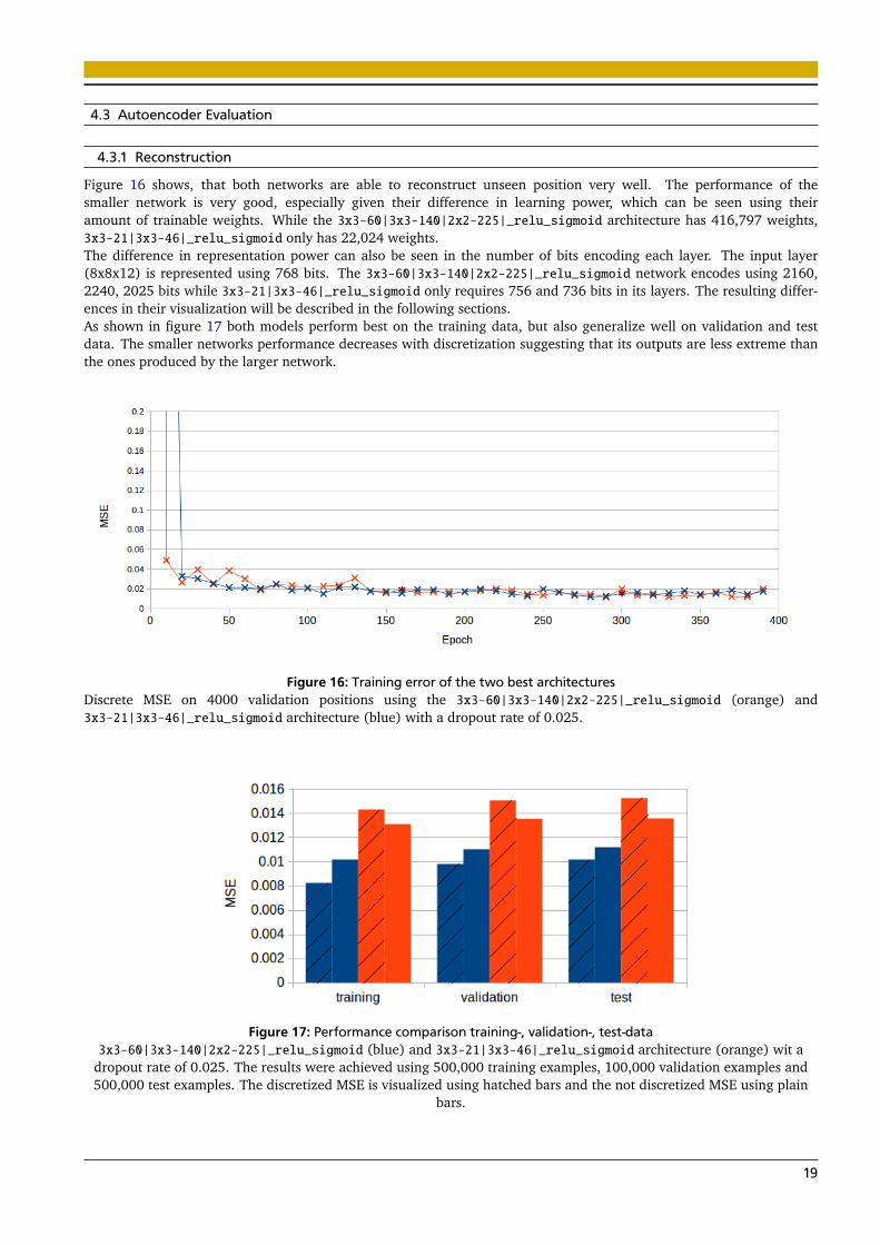
Figure 16 shows, that both networks are able to reconstruct unseen position very well. The performance of thesmaller network is very good, especially given their difference in learning power, which can be seen using theiramount of trainable weights. While the 3x3-60|3x3-140|2x2-225|_relu_sigmoid architecture has 416,797 weights,3x3-21|3x3-46|_relu_sigmoid only has 22,024 weights.The difference in representation power can also be seen in the number of bits encoding each layer. The input layer(8x8x12) is represented using 768 bits. The 3x3-60|3x3-140|2x2-225|_relu_sigmoid network encodes using 2160,2240, 2025 bits while 3x3-21|3x3-46|_relu_sigmoid only requires 756 and 736 bits in its layers. The resulting differ-ences in their visualization will be described in the following sections.As shown in figure 17 both models perform best on the training data, but also generalize well on validation and testdata. The smaller networks performance decreases with discretization suggesting that its outputs are less extreme thanthe ones produced by the larger network.

Figure 16: Training error of the two best architecturesDiscrete MSE on 4000 validation positions using the 3x3-60|3x3-140|2x2-225|_relu_sigmoid (orange) and3x3-21|3x3-46|_relu_sigmoid architecture (blue) with a dropout rate of 0.025.

Figure 17: Performance comparison training-, validation-, test-data3x3-60|3x3-140|2x2-225|_relu_sigmoid (blue) and 3x3-21|3x3-46|_relu_sigmoid architecture (orange) wit a

dropout rate of 0.025. The results were achieved using 500,000 training examples, 100,000 validation examples and500,000 test examples. The discretized MSE is visualized using hatched bars and the not discretized MSE using plain

bars.

19

4.3.2 Visualization

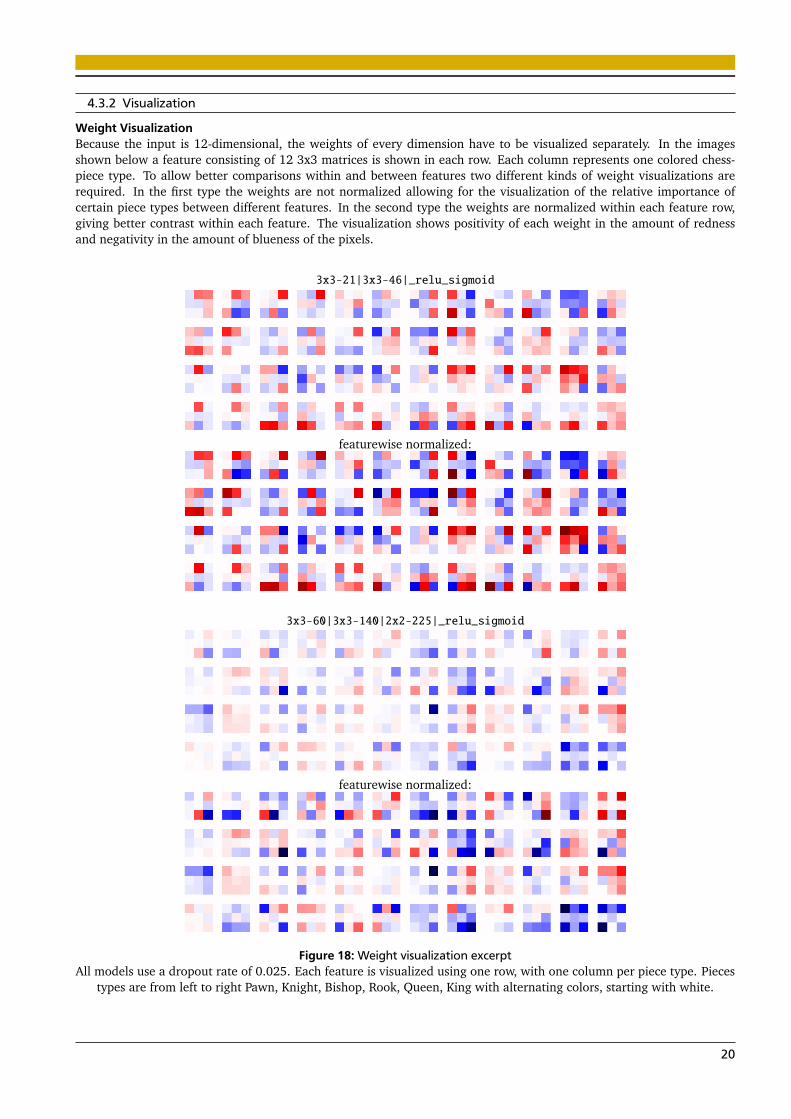
Weight VisualizationBecause the input is 12-dimensional, the weights of every dimension have to be visualized separately. In the imagesshown below a feature consisting of 12 3x3 matrices is shown in each row. Each column represents one colored chess-piece type. To allow better comparisons within and between features two different kinds of weight visualizations arerequired. In the first type the weights are not normalized allowing for the visualization of the relative importance ofcertain piece types between different features. In the second type the weights are normalized within each feature row,giving better contrast within each feature. The visualization shows positivity of each weight in the amount of rednessand negativity in the amount of blueness of the pixels.

3x3-21|3x3-46|_relu_sigmoid

featurewise normalized:

3x3-60|3x3-140|2x2-225|_relu_sigmoid

featurewise normalized:

Figure 18: Weight visualization excerptAll models use a dropout rate of 0.025. Each feature is visualized using one row, with one column per piece type. Pieces

types are from left to right Pawn, Knight, Bishop, Rook, Queen, King with alternating colors, starting with white.

20

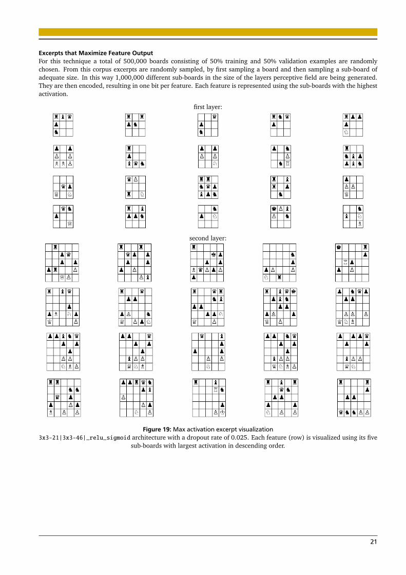
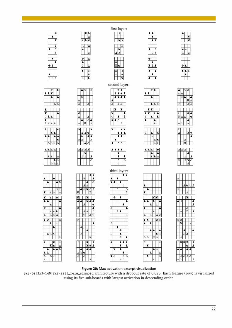
Excerpts that Maximize Feature OutputFor this technique a total of 500,000 boards consisting of 50% training and 50% validation examples are randomlychosen. From this corpus excerpts are randomly sampled, by first sampling a board and then sampling a sub-board ofadequate size. In this way 1,000,000 different sub-boards in the size of the layers perceptive field are being generated.They are then encoded, resulting in one bit per feature. Each feature is represented using the sub-boards with the highestactivation.

first layer:

second layer:

Figure 19: Max activation excerpt visualization3x3-21|3x3-46|_relu_sigmoid architecture with a dropout rate of 0.025. Each feature (row) is visualized using its five

sub-boards with largest activation in descending order.

21

first layer:

second layer:

third layer:

Figure 20: Max activation excerpt visualization3x3-60|3x3-140|2x2-225|_relu_sigmoid architecture with a dropout rate of 0.025. Each feature (row) is visualized

using its five sub-boards with largest activation in descending order.

22

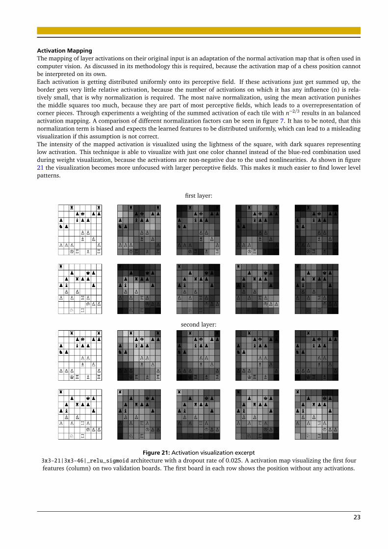
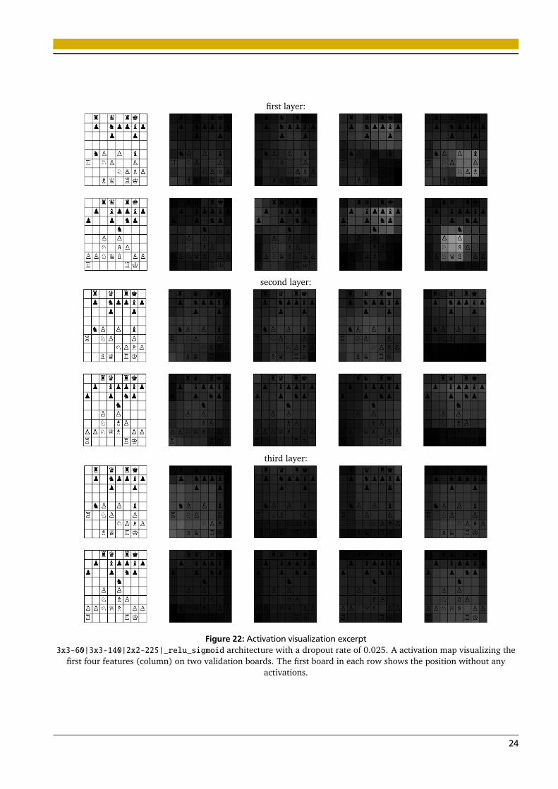
Activation MappingThe mapping of layer activations on their original input is an adaptation of the normal activation map that is often used incomputer vision. As discussed in its methodology this is required, because the activation map of a chess position cannotbe interpreted on its own.Each activation is getting distributed uniformly onto its perceptive field. If these activations just get summed up, theborder gets very little relative activation, because the number of activations on which it has any influence (n) is rela-tively small, that is why normalization is required. The most naive normalization, using the mean activation punishesthe middle squares too much, because they are part of most perceptive fields, which leads to a overrepresentation ofcorner pieces. Through experiments a weighting of the summed activation of each tile with n−2/3 results in an balancedactivation mapping. A comparison of different normalization factors can be seen in figure 7. It has to be noted, that thisnormalization term is biased and expects the learned features to be distributed uniformly, which can lead to a misleadingvisualization if this assumption is not correct.The intensity of the mapped activation is visualized using the lightness of the square, with dark squares representinglow activation. This technique is able to visualize with just one color channel instead of the blue-red combination usedduring weight visualization, because the activations are non-negative due to the used nonlinearities. As shown in figure21 the visualization becomes more unfocused with larger perceptive fields. This makes it much easier to find lower levelpatterns.

first layer:

second layer:

Figure 21: Activation visualization excerpt3x3-21|3x3-46|_relu_sigmoid architecture with a dropout rate of 0.025. A activation map visualizing the first fourfeatures (column) on two validation boards. The first board in each row shows the position without any activations.

23

first layer:

second layer:

third layer:

Figure 22: Activation visualization excerpt3x3-60|3x3-140|2x2-225|_relu_sigmoid architecture with a dropout rate of 0.025. A activation map visualizing the

first four features (column) on two validation boards. The first board in each row shows the position without anyactivations.

24

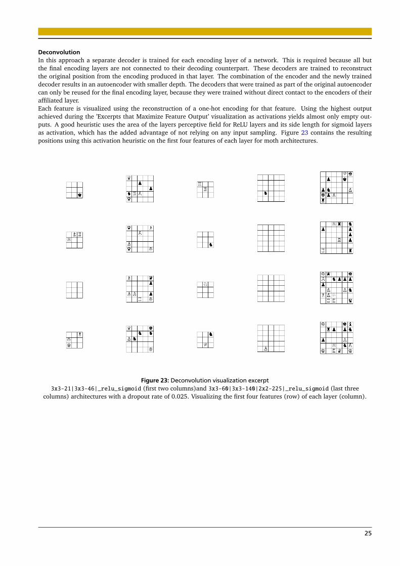
DeconvolutionIn this approach a separate decoder is trained for each encoding layer of a network. This is required because all butthe final encoding layers are not connected to their decoding counterpart. These decoders are trained to reconstructthe original position from the encoding produced in that layer. The combination of the encoder and the newly traineddecoder results in an autoencoder with smaller depth. The decoders that were trained as part of the original autoencodercan only be reused for the final encoding layer, because they were trained without direct contact to the encoders of theiraffiliated layer.Each feature is visualized using the reconstruction of a one-hot encoding for that feature. Using the highest outputachieved during the ’Excerpts that Maximize Feature Output’ visualization as activations yields almost only empty out-puts. A good heuristic uses the area of the layers perceptive field for ReLU layers and its side length for sigmoid layersas activation, which has the added advantage of not relying on any input sampling. Figure 23 contains the resultingpositions using this activation heuristic on the first four features of each layer for moth architectures.

Figure 23: Deconvolution visualization excerpt3x3-21|3x3-46|_relu_sigmoid (first two columns)and 3x3-60|3x3-140|2x2-225|_relu_sigmoid (last three

columns) architectures with a dropout rate of 0.025. Visualizing the first four features (row) of each layer (column).

25

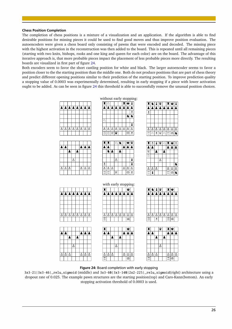
Chess Position CompletionThe completion of chess positions is a mixture of a visualization and an application. If the algorithm is able to finddesirable positions for missing pieces it could be used to find good moves and thus improve position evaluation. Theautoencoders were given a chess board only consisting of pawns that were encoded and decoded. The missing piecewith the highest activation in the reconstruction was then added to the board. This is repeated until all remaining pieces(starting with two knits, bishops, rooks and one king and queen for each color) are on the board. The advantage of thisiterative approach is, that more probable pieces impact the placement of less probable pieces more directly. The resultingboards are visualized in first part of figure 24.Both encoders seem to favor the short castling position for white and black. The larger autoencoder seems to favor aposition closer to the the starting position than the middle one. Both do not produce positions that are part of chess theoryand predict different opening positions similar to their prediction of the starting position. To improve prediction qualitya stopping value of 0.0003 was experimentally determined, resulting in early stopping if a piece with lower activationought to be added. As can be seen in figure 24 this threshold is able to successfully remove the unusual position choices.

without early stopping:

with early stopping:

Figure 24: Board completion with early stopping3x3-21|3x3-46|_relu_sigmoid (middle) and 3x3-60|3x3-140|2x2-225|_relu_sigmoid(right) architecture using adropout rate of 0.025. The example pawn structures are the starting position(top) and Caro-Kann(bottom). An early

stopping activation threshold of 0.0003 is used.

26

4.3.3 Application

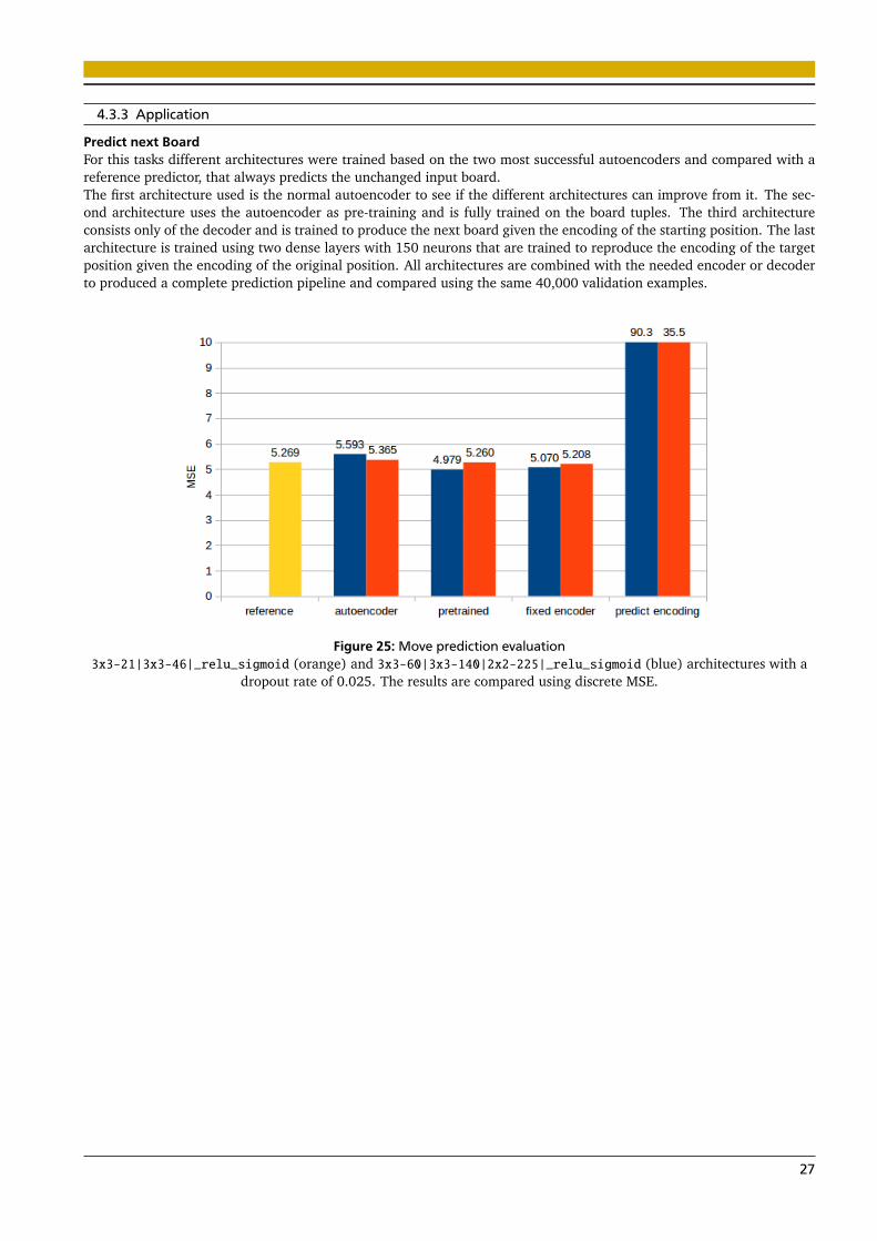
Predict next BoardFor this tasks different architectures were trained based on the two most successful autoencoders and compared with areference predictor, that always predicts the unchanged input board.The first architecture used is the normal autoencoder to see if the different architectures can improve from it. The sec-ond architecture uses the autoencoder as pre-training and is fully trained on the board tuples. The third architectureconsists only of the decoder and is trained to produce the next board given the encoding of the starting position. The lastarchitecture is trained using two dense layers with 150 neurons that are trained to reproduce the encoding of the targetposition given the encoding of the original position. All architectures are combined with the needed encoder or decoderto produced a complete prediction pipeline and compared using the same 40,000 validation examples.

Figure 25: Move prediction evaluation3x3-21|3x3-46|_relu_sigmoid (orange) and 3x3-60|3x3-140|2x2-225|_relu_sigmoid (blue) architectures with a

dropout rate of 0.025. The results are compared using discrete MSE.

27

4.4 Evaluation

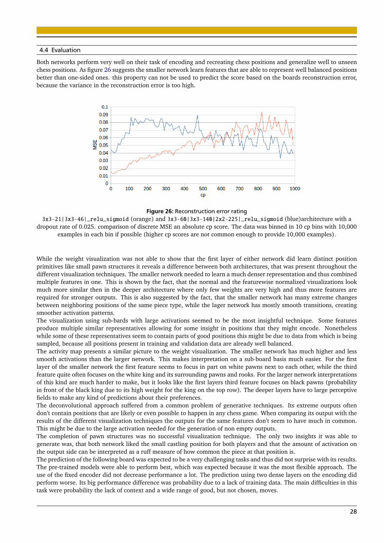
Both networks perform very well on their task of encoding and recreating chess positions and generalize well to unseenchess positions. As figure 26 suggests the smaller network learn features that are able to represent well balanced positionsbetter than one-sided ones. this property can not be used to predict the score based on the boards reconstruction error,because the variance in the reconstruction error is too high.

Figure 26: Reconstruction error rating3x3-21|3x3-46|_relu_sigmoid (orange) and 3x3-60|3x3-140|2x2-225|_relu_sigmoid (blue)architecture with a

dropout rate of 0.025. comparison of discrete MSE an absolute cp score. The data was binned in 10 cp bins with 10,000examples in each bin if possible (higher cp scores are not common enough to provide 10,000 examples).

While the weight visualization was not able to show that the first layer of either network did learn distinct positionprimitives like small pawn structures it reveals a difference between both architectures, that was present throughout thedifferent visualization techniques. The smaller network needed to learn a much denser representation and thus combinedmultiple features in one. This is shown by the fact, that the normal and the featurewise normalized visualizations lookmuch more similar then in the deeper architecture where only few weights are very high and thus more features arerequired for stronger outputs. This is also suggested by the fact, that the smaller network has many extreme changesbetween neighboring positions of the same piece type, while the lager network has mostly smooth transitions, creatingsmoother activation patterns.The visualization using sub-bards with large activations seemed to be the most insightful technique. Some featuresproduce multiple similar representatives allowing for some insight in positions that they might encode. Nonethelesswhile some of these representatives seem to contain parts of good positions this might be due to data from which is beingsampled, because all positions present in training and validation data are already well balanced.The activity map presents a similar picture to the weight visualization. The smaller network has much higher and lesssmooth activations than the larger network. This makes interpretation on a sub-board basis much easier. For the firstlayer of the smaller network the first feature seems to focus in part on white pawns next to each other, while the thirdfeature quite often focuses on the white king and its surrounding pawns and rooks. For the larger network interpretationsof this kind are much harder to make, but it looks like the first layers third feature focuses on black pawns (probabilityin front of the black king due to its high weight for the king on the top row). The deeper layers have to large perceptivefields to make any kind of predictions about their preferences.The deconvolutional approach suffered from a common problem of generative techniques. Its extreme outputs oftendon’t contain positions that are likely or even possible to happen in any chess game. When comparing its output with theresults of the different visualization techniques the outputs for the same features don’t seem to have much in common.This might be due to the large activation needed for the generation of non empty outputs.The completion of pawn structures was no successful visualization technique. The only two insights it was able togenerate was, that both network liked the small castling position for both players and that the amount of activation onthe output side can be interpreted as a ruff measure of how common the piece at that position is.The prediction of the following board was expected to be a very challenging tasks and thus did not surprise with its results.The pre-trained models were able to perform best, which was expected because it was the most flexible approach. Theuse of the fixed encoder did not decrease performance a lot. The prediction using two dense layers on the encoding didperform worse. Its big performance difference was probability due to a lack of training data. The main difficulties in thistask were probability the lack of context and a wide range of good, but not chosen, moves.

28

5 Conclusion

As elaborated in the previous section, the features learned by the autoencoders don’t seem to consist of human inter-pretable position primitives. This might be in part due to an undesirable property of bitmaps that was mentioned by Lai etal. [15]. When using bitmaps as input representation the distance between two boards is measured in their total bitwisedifference, which does not provide the best information about how different both positions really are, because it ratesthe shift of a piece by one tile worse than the disappearance of that piece. This is why giraffe[15] uses a list of piece co-ordinates as its input representation and omits the grid structures required for convolutional approaches. DeepChess[6]uses bitmaps as their input in combination with a purely dense architecture. This approach requires them to use muchmore training data (2 · 1012 training pairs) than the 3 · 106 boards used in this thesis.The feature visualization methods can give an idea about the lower layer features when used in combination with eachother. Features in higher layers are too spread out and complex to allow for any real insight. The small size and infor-mation density of the input makes chess boards a difficult application for convolutional approaches due to their depthlimiting and information dense properties. The features learned by both architectures don’t seem to consist of any com-monly known and recognizable structures.The prediction of the next position seems to require a more tailored approach and likely more training data. The visu-alization techniques could also be further developed by expanding the ’excerpts that maximize feature output’ methodwith a board combination algorithm or adding an optimization based feature maximization approach.Another approach could be the implementation of the DeepChess architecture using a convolutional network. Thismethod could be used to evaluate the viability of convolutions in the chess domain for a task with an existing referencearchitecture. If the convolutional architecture is able to successfully play chess, the developed visualizations can be usedto investigate the learned features.

29

References

[1] Marcin Andrychowicz, Misha Denil, Sergio Gomez, Matthew W Hoffman, David Pfau, Tom Schaul, and Nando deFreitas. “Learning to learn by gradient descent by gradient descent”. In: Advances in Neural Information ProcessingSystems. 2016, pp. 3981–3989.

[2] Yoshua Bengio. “Learning deep architectures for AI”. In: Foundations and trends in Machine Learning 2.1 (2009),pp. 1–127.

[3] Yoshua Bengio, Aaron C Courville, and Pascal Vincent. “Unsupervised feature learning and deep learning: A reviewand new perspectives”. In: CoRR, abs/1206.5538 1 (2012).

[4] Christopher M. Bishop. Pattern Recognition and Machine Learning (Information Science and Statistics). Secaucus,NJ, USA: Springer-Verlag New York, Inc., 2006. ISBN: 0387310738.

[5] Balázs Csanád Csáji. “Approximation with Artificial Neural Networks”. MA thesis. 2001.

[6] Omid E David, Nathan S Netanyahu, and Lior Wolf. “DeepChess: End-to-End Deep Neural Network for AutomaticLearning in Chess”. In: International Conference on Artificial Neural Networks. Springer. 2016, pp. 88–96.

[7] Dumitru Erhan, Yoshua Bengio, Aaron Courville, Pierre-Antoine Manzagol, Pascal Vincent, and Samy Bengio.“Why does unsupervised pre-training help deep learning?” In: Journal of Machine Learning Research 11.Feb (2010),pp. 625–660.

[8] Ross Girshick, Jeff Donahue, Trevor Darrell, and Jitendra Malik. “Rich feature hierarchies for accurate object detec-tion and semantic segmentation”. In: Proceedings of the IEEE conference on computer vision and pattern recognition.2014, pp. 580–587.

[9] Xavier Glorot, Antoine Bordes, and Yoshua Bengio. “Deep sparse rectifier neural networks”. In: Proceedings of theFourteenth International Conference on Artificial Intelligence and Statistics. 2011, pp. 315–323.

[10] Ian Goodfellow, Yoshua Bengio, and Aaron Courville. Deep Learning. http://www.deeplearningbook.org. MITPress, 2016.

[11] Geoffrey E. Hinton, Nitish Srivastava, Alex Krizhevsky, Ilya Sutskever, and Ruslan Salakhutdinov. “Improvingneural networks by preventing co-adaptation of feature detectors”. In: CoRR abs/1207.0580 (2012).

[12] Geoffrey Hinton, Li Deng, Dong Yu, George E Dahl, Abdel-rahman Mohamed, Navdeep Jaitly, Andrew Senior,Vincent Vanhoucke, Patrick Nguyen, Tara N Sainath, et al. “Deep neural networks for acoustic modeling in speechrecognition: The shared views of four research groups”. In: IEEE Signal Processing Magazine 29.6 (2012), pp. 82–97.

[13] Diederik P. Kingma and Jimmy Ba. “Adam: A Method for Stochastic Optimization”. In: CoRR abs/1412.6980(2014). arXiv: 1412.6980. URL: http://arxiv.org/abs/1412.6980.

[14] Alex Krizhevsky, Ilya Sutskever, and Geoffrey E Hinton. “Imagenet classification with deep convolutional neuralnetworks”. In: Advances in neural information processing systems. 2012, pp. 1097–1105.

[15] Matthew Lai. “Giraffe: Using Deep Reinforcement Learning to Play Chess”. In: CoRR abs/1509.01549 (2015). URL:http://arxiv.org/abs/1509.01549.

[16] Olga Russakovsky, Jia Deng, Hao Su, Jonathan Krause, Sanjeev Satheesh, Sean Ma, Zhiheng Huang, Andrej Karpa-thy, Aditya Khosla, Michael Bernstein, Alexander C. Berg, and Li Fei-Fei. “ImageNet Large Scale Visual RecognitionChallenge”. In: International Journal of Computer Vision (IJCV) 115.3 (2015), pp. 211–252. DOI: 10.1007/s11263-015-0816-y.

[17] David Silver, Aja Huang, Chris J Maddison, Arthur Guez, Laurent Sifre, George Van Den Driessche, Julian Schrit-twieser, Ioannis Antonoglou, Veda Panneershelvam, Marc Lanctot, et al. “Mastering the game of Go with deepneural networks and tree search”. In: Nature 529.7587 (2016), pp. 484–489.

[18] Stefan Steinerberger. “On the number of positions in chess without promotion”. In: International Journal of GameTheory 44.3 (Aug. 2015), pp. 761–767. DOI: 10.1007/s00182-014-0453-7. URL: https://doi.org/10.1007/s00182-014-0453-7.

[19] Christian Szegedy, Sergey Ioffe, and Vincent Vanhoucke. “Inception-v4, Inception-ResNet and the Impact of Resid-ual Connections on Learning”. In: CoRR abs/1602.07261 (2016). URL: http://arxiv.org/abs/1602.07261.

[20] Eliezer Yudkowsky. “Artificial intelligence as a positive and negative factor in global risk”. In: Global catastrophicrisks 1.303 (2008), p. 184.

[21] Matthew D Zeiler and Rob Fergus. “Visualizing and understanding convolutional networks”. In: European confer-ence on computer vision. Springer. 2014, pp. 818–833.

30

List of Figures

1 Perceptron . . . . . . . . . . . . . . . . . . . . . . . . . . . . . . . . . . . . . . . . . . . . . . . . . . . . . . . . . . . . 42 Fully connected two layer neural network . . . . . . . . . . . . . . . . . . . . . . . . . . . . . . . . . . . . . . . . . 43 Example autoencoder nomenclature . . . . . . . . . . . . . . . . . . . . . . . . . . . . . . . . . . . . . . . . . . . . 94 Evaluation example . . . . . . . . . . . . . . . . . . . . . . . . . . . . . . . . . . . . . . . . . . . . . . . . . . . . . . . 105 Weight visualization example . . . . . . . . . . . . . . . . . . . . . . . . . . . . . . . . . . . . . . . . . . . . . . . . . 116 Maximize feature output visualization example . . . . . . . . . . . . . . . . . . . . . . . . . . . . . . . . . . . . . . 117 Activation mapping visualization example . . . . . . . . . . . . . . . . . . . . . . . . . . . . . . . . . . . . . . . . . 128 Deconvolution visualization example . . . . . . . . . . . . . . . . . . . . . . . . . . . . . . . . . . . . . . . . . . . . 129 Chess position completion example . . . . . . . . . . . . . . . . . . . . . . . . . . . . . . . . . . . . . . . . . . . . . 1310 PGN excerpt . . . . . . . . . . . . . . . . . . . . . . . . . . . . . . . . . . . . . . . . . . . . . . . . . . . . . . . . . . . 1411 Chess position . . . . . . . . . . . . . . . . . . . . . . . . . . . . . . . . . . . . . . . . . . . . . . . . . . . . . . . . . . 1412 FEN . . . . . . . . . . . . . . . . . . . . . . . . . . . . . . . . . . . . . . . . . . . . . . . . . . . . . . . . . . . . . . . . 1513 Bitmap . . . . . . . . . . . . . . . . . . . . . . . . . . . . . . . . . . . . . . . . . . . . . . . . . . . . . . . . . . . . . . . 1514 Dropout rate comparison . . . . . . . . . . . . . . . . . . . . . . . . . . . . . . . . . . . . . . . . . . . . . . . . . . . 1615 Noise comparison . . . . . . . . . . . . . . . . . . . . . . . . . . . . . . . . . . . . . . . . . . . . . . . . . . . . . . . . 1716 Training error of the two best architectures . . . . . . . . . . . . . . . . . . . . . . . . . . . . . . . . . . . . . . . . 1917 Performance comparison training-, validation-, test-data . . . . . . . . . . . . . . . . . . . . . . . . . . . . . . . . 1918 Weight visualization excerpt . . . . . . . . . . . . . . . . . . . . . . . . . . . . . . . . . . . . . . . . . . . . . . . . . 2019 Max activation excerpt visualization . . . . . . . . . . . . . . . . . . . . . . . . . . . . . . . . . . . . . . . . . . . . . 2120 Max activation excerpt visualization . . . . . . . . . . . . . . . . . . . . . . . . . . . . . . . . . . . . . . . . . . . . . 2221 Activation visualization excerpt . . . . . . . . . . . . . . . . . . . . . . . . . . . . . . . . . . . . . . . . . . . . . . . 2322 Activation visualization excerpt . . . . . . . . . . . . . . . . . . . . . . . . . . . . . . . . . . . . . . . . . . . . . . . 2423 Deconvolution visualization excerpt . . . . . . . . . . . . . . . . . . . . . . . . . . . . . . . . . . . . . . . . . . . . . 2524 Board completion with early stopping . . . . . . . . . . . . . . . . . . . . . . . . . . . . . . . . . . . . . . . . . . . 2625 Move prediction evaluation . . . . . . . . . . . . . . . . . . . . . . . . . . . . . . . . . . . . . . . . . . . . . . . . . . 2726 Reconstruction error rating . . . . . . . . . . . . . . . . . . . . . . . . . . . . . . . . . . . . . . . . . . . . . . . . . . 28

List of Tables

1 Activation comparison . . . . . . . . . . . . . . . . . . . . . . . . . . . . . . . . . . . . . . . . . . . . . . . . . . . . . 172 evaluation of different layouts . . . . . . . . . . . . . . . . . . . . . . . . . . . . . . . . . . . . . . . . . . . . . . . . 18

31